applications of geographical information systems (gis) for spatial
TRANSCRIPT
Aquacultural Engineering 23 (2000) 233–278
Applications of geographical informationsystems (GIS) for spatial decision support in
aquaculture
Shree S. Nath a,*, John P. Bolte b, Lindsay G. Ross c,Jose Aguilar-Manjarrez d
a Skillings-Connolly, Inc., 5016 Lacey Boule6ard S.E., Lacey, WA 98503, USAb Department of Bioresource Engineering, Oregon State Uni6ersity, Cor6allis, OR 97331, USA
c Institute of Aquaculture, Uni6ersity of Stirling, Stirling FK9 4LA, UKd Food and Agricultural Organisation of the U.N, Viale delle Termi di Caracalla, 00100 Rome, Italy
Received 1 September 1999; accepted 2 October 1999
Abstract
Geographical information systems (GIS) are becoming an increasingly integral componentof natural resource management activities worldwide. However, despite some indication thatthese tools are receiving attention within the aquaculture community, their deployment forspatial decision support in this domain continues to be very slow. This situation isattributable to a number of constraints including a lack of appreciation of the technology,limited understanding of GIS principles and associated methodology, and inadequateorganizational commitment to ensure continuity of these spatial decision support tools. Thispaper analyzes these constraints in depth, and includes reviews of basic GIS terminology,methodology, case studies in aquaculture and future trends. The section on GIS terminologyaddresses the two fundamental types of GIS (raster and vector), and discusses aspects relatedto the visualization of outcomes. With regard to GIS methodology, the argument is made forclose involvement of end users, subject matter specialists and analysts in all projects. Auser-driven framework, which involves seven phases, to support this process is presentedtogether with details of the degree of involvement of each category of personnel, associatedactivities and analytical procedures. The section on case studies reviews in considerable detailfour aquaculture applications which are demonstrative of the extent to which GIS can bedeployed, indicate the range in complexity of analytical methods used, provide insight into
www.elsevier.nl/locate/aqua-online
* Corresponding author. Tel.: +1-360-4913399; fax: +1-360-4913857.E-mail address: [email protected] (S.S. Nath)
0144-8609/00/$ - see front matter © 2000 Elsevier Science B.V. All rights reserved.PII: S0144 -8609 (00 )00051 -0
234 S.S. Nath et al. / Aquacultural Engineering 23 (2000) 233–278
issues associated with data procurement and handling, and demonstrate the diversity of GISpackages that are available. Finally, the section on the future of GIS examines the directionin which the technology is moving, emerging trends with regard to analytical methods, andchallenges that need to be addressed if GIS is to realize its full potential as a spatial decisionsupport tool for aquaculture. © 223 Elsevier Science B.V. All rights reserved.
Keywords: GIS; Aquaculture; Spacial decision support
1. Introduction
The rapid growth of aquaculture worldwide has stimulated considerable interestamong international technical assistance organizations and national-level govern-mental agencies in countries where fish culture is still in its infancy, and has resultedin increased concerns about its sustainability in countries where the industry is wellestablished. Planning activities to promote and monitor the growth of aquaculturein individual countries (or larger regions) inherently have a spatial componentbecause of the differences among biophysical and socio-economic characteristicsfrom location to location. Biophysical characteristics may include criteria pertinentto water quality (e.g. temperature, dissolved oxygen, alkalinity/salinity, turbidity,and pollutant concentrations), water quantity (e.g. volume and seasonal profiles ofavailability), soil type (e.g. slope, structural suitability, water retention capacity andchemical nature) and climate (e.g. rainfall distribution, air temperature, wind speedand relative humidity). Socio-economic characteristics that may be considered inaquaculture development include administrative regulations, competing resourceuses, market conditions (e.g. demand for fishery products and accessibility tomarkets), infrastucture support, and availability of technical expertise. The spatialinformation needs for decision-makers who evaluate such biophysical and socio-economic characteristics as part of aquaculture planning efforts can be well servedby geographical information systems (GIS; Kapetsky and Travaglia, 1995).
Moreover, it is often the case that governmental agencies involved with issuingnew aquaculture permits need to perform spatial analysis on a proposed site toassess its potential environmental, economic and social impacts on other locations.This situation is analogous to the need for monitoring existing operations in termsof environmental and/or other impacts. As noted by Osleeb and Kahn (1998), thesedecision support needs cannot be effectively addressed without the use of GIS.Finally, Kapetsky and Travaglia (1995) also point out that the individual investorinterested in aquaculture development also requires spatial information particularlyat the time of site selection from among a range of alternative locations withdifferent biophysical and socio-economic characteristics. GIS is potentially a pow-erful tool for assisting this class of decision-makers, and is already being effectivelyused for such purposes in some places (Carswell, 1998; LUCO, 1998; Arnold et al.,2000) where advanced capabilities in terms of infrastructure and trained personnelexists. In general, however, increased deployment of GIS for practical decision-making in aquaculture is hampered by several constraints including: (1) a lack of
235S.S. Nath et al. / Aquacultural Engineering 23 (2000) 233–278
appreciation of the benefits of such systems on the part of key decision-makers; (2)limited understanding about GIS principles and associated methodology; (3) inade-quate administrative support to ensure GIS continuity among organizations; and(4) poor levels of interaction among GIS analysts, subject matter specialists and endusers of the technology (see also Kapetsky and Travaglia, 1995).
The primary goals of this overview are to examine the above constraints in depth,and to supplement previous reviews of GIS applications in aquaculture (Meadenand Kapetsky, 1991; Kapetsky and Travaglia, 1995; Aguilar-Manjarrez, 1996;Ross, 1998). Our overview includes an introduction to GIS terminology andmethodology, topics that are relatively well documented in the literature (Burrough,1986), but to which personnel in aquaculture have had limited exposure, especiallyfrom the perspective of GIS as a tool for practical decision-making. A summary ofselected cases where such tools have been applied in aquaculture is also provided.Finally, a section of the paper focuses on the future of GIS in aquaculture, andrecommendations for its continued use.
2. GIS terminology
GIS is an integrated assembly of computer hardware, software, geographic dataand personnel designed to efficiently acquire, store, manipulate, retrieve, analyze,display and report all forms of geographically referenced information gearedtowards a particular set of purposes (Burrough, 1986; Kapetsky and Travaglia,1995). An excellent introduction to GIS terminology, maintained by the Associa-tion of Geographic Information, is available on the World Wide Web (WWW) athttp://www.geo.ed.ac.uk/root/agidict/html/welcome.html.
There are essentially two types of GIS — vector and raster systems. Thesesystems differ in the manner by which spatial data are represented and stored.Burrough (1986) and Meaden and Kapetsky (1991) provide useful comparisons ofvector and raster systems in summary form. In both systems, a ‘geographiccoordinate system’ is used to represent space. Many coordinate systems have beendefined, ranging from simple Cartesian X-Y grids to spatial representations thatcorrespond to the real world such as latitude/longitude pairings, State Planecoordinates or the Universal Transverse Mercator system coordinate system (Bur-rough, 1986; Thompson, 1998).
2.1. Vector GIS
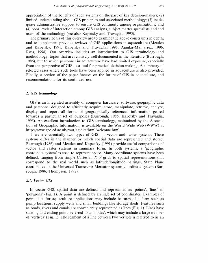
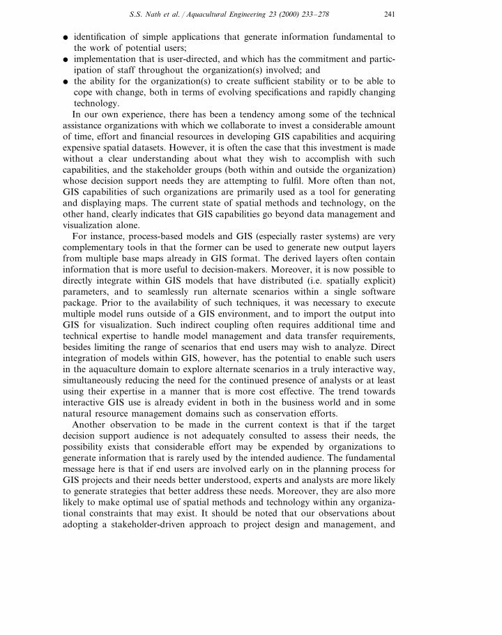
In vector GIS, spatial data are defined and represented as ‘points’, ‘lines’ or‘polygons’ (Fig. 1). A point is defined by a single set of coordinates. Examples ofpoint data for aquaculture applications may include features of a farm such aspump locations, supply wells and small buildings like storage sheds. Features suchas roads, rivers and canals are conveniently represented as lines (Fig. 1). Lines havestarting and ending points referred to as ‘nodes’, which may include a large numberof ‘vertices’ (Fig. 1). The segment of a line between two vertices is referred to as an
236 S.S. Nath et al. / Aquacultural Engineering 23 (2000) 233–278
‘arc’. Polygons are used in GIS to represent enclosed areas (Fig. 1). A polygonconsists of a number of lines, but is distinguished by the characteristic that itsstarting and ending nodes are the same. For aquaculture applications, examples ofpolygons include a reservoir, a certain soil class, and a distinct type of landclassification (e.g. a mangrove forest). Based on the coordinate system used, avector GIS knows where the spatial feature (point, line or polygon) exists (i.e. itsabsolute location), and its relationship to other features (topology or relativelocation). As an example, a GIS would thus be aware that a reservoir supplyingwater to a fish farm is located north of the farm ponds.
After spatial features are represented in vector GIS, their associated propertiescan be specified in a separate database. As an example, properties of a soil polygonsuch as pH, bulk density, cation exchange capacity, and infiltration rate can bearchived in a database. These properties are often referred to as ‘themes’, which canbe presented in so called ‘thematic maps’. Vector GIS lend themselves well to theuse of relational databases because once the spatial features are specified (once),any amount of related data can be associated with them. The term ‘coverage’ isused in the GIS literature to refer to the combination of a geographically referencedfeature and its associated data. Thus, a ‘stream coverage’ would refer to the line ina vector GIS that represents its course, and the associated data such as flow rates,temperature, water quality characteristics, and withdrawal rates (and possiblyspatial locations) for different uses.
2.2. Raster GIS
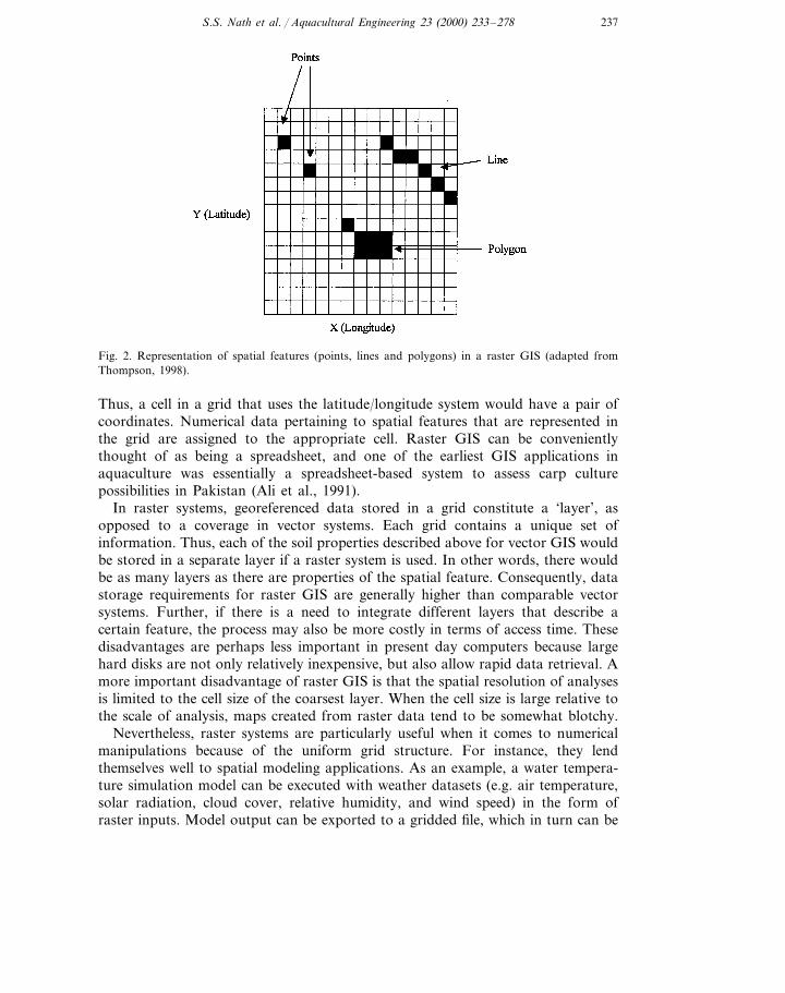
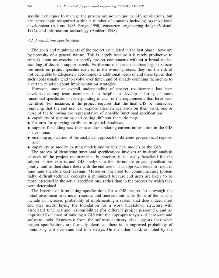
In a raster GIS, space is represented by a uniform grid, each cell of which isassigned a unique descriptor depending on the coordinate system used (Fig. 2).
Fig. 1. Representation of spatial features (points, lines and polygons) in a vector GIS (adapted fromThompson, 1998).
237S.S. Nath et al. / Aquacultural Engineering 23 (2000) 233–278
Fig. 2. Representation of spatial features (points, lines and polygons) in a raster GIS (adapted fromThompson, 1998).
Thus, a cell in a grid that uses the latitude/longitude system would have a pair ofcoordinates. Numerical data pertaining to spatial features that are represented inthe grid are assigned to the appropriate cell. Raster GIS can be convenientlythought of as being a spreadsheet, and one of the earliest GIS applications inaquaculture was essentially a spreadsheet-based system to assess carp culturepossibilities in Pakistan (Ali et al., 1991).
In raster systems, georeferenced data stored in a grid constitute a ‘layer’, asopposed to a coverage in vector systems. Each grid contains a unique set ofinformation. Thus, each of the soil properties described above for vector GIS wouldbe stored in a separate layer if a raster system is used. In other words, there wouldbe as many layers as there are properties of the spatial feature. Consequently, datastorage requirements for raster GIS are generally higher than comparable vectorsystems. Further, if there is a need to integrate different layers that describe acertain feature, the process may also be more costly in terms of access time. Thesedisadvantages are perhaps less important in present day computers because largehard disks are not only relatively inexpensive, but also allow rapid data retrieval. Amore important disadvantage of raster GIS is that the spatial resolution of analysesis limited to the cell size of the coarsest layer. When the cell size is large relative tothe scale of analysis, maps created from raster data tend to be somewhat blotchy.
Nevertheless, raster systems are particularly useful when it comes to numericalmanipulations because of the uniform grid structure. For instance, they lendthemselves well to spatial modeling applications. As an example, a water tempera-ture simulation model can be executed with weather datasets (e.g. air temperature,solar radiation, cloud cover, relative humidity, and wind speed) in the form ofraster inputs. Model output can be exported to a gridded file, which in turn can be
238 S.S. Nath et al. / Aquacultural Engineering 23 (2000) 233–278
imported into raster systems for further classification and display (Kapetsky andNath, 1997). Similarly, raster GIS can be used to model effluents discharged byaquaculture operations into natural water bodies by applying appropriate equationsto cells in the spatial grid (Perez-Martinez, 1997). Another advantage of raster GISis that remote sensed data (which are usually stored in raster format) can often bedirectly imported into the software and immediately become available for use(Burrough, 1986).
2.3. Analytical scope, reporting and 6isualization
One of the powerful features of both vector and raster GIS packages is thatstatistical summaries of layers/coverages, model stages or outcomes can easily beobtained. Statistical data can include area, perimeter and other quantitative esti-mates, including reports of variance and comparison among images. A furtherpowerful analytical tool that aids understanding of outcomes is visualization ofoutcomes through graphical representation in the form of 2D and 3D maps. Forexample, entire landscapes and watersheds can be viewed in three dimensions,which is very valuable in terms of evaluating spatial impacts of alternative deci-sions. Techniques have also been developed to integrate GIS with additional toolssuch as group support systems, that allow interactive scenario development andevaluation, and support communication among stakeholders via a local areanetwork (LAN; Faber et al., 1997). There is also currently rapid development anddeployment of Internet-enabled GIS tools, which allow a wider community ofdecision makers to have instant access to spatial data. All of these tools areconstantly being added to GIS packages and are of great value if appropriatelyused. Presently available tools include Arc/Explorer and Internet Map Server (fromESRI, Inc) and MapXtreme (from MapInfo Corporation). Because GIS technologyis evolving at a very rapid rate, we have chosen not to evaluate specific products.Information about GIS and related tools are, however, available from various Websites including: http://www.utexas.edu/depts/grg/virtdept/resources/vendors/ven-dors.htm and http://www.gislinx.com/. Guidelines for selecting GIS tools areavailable in: Burrough (1986), Meaden and Kapetsky (1991) and Burrough andMcDonnell (1998).
3. GIS methodology
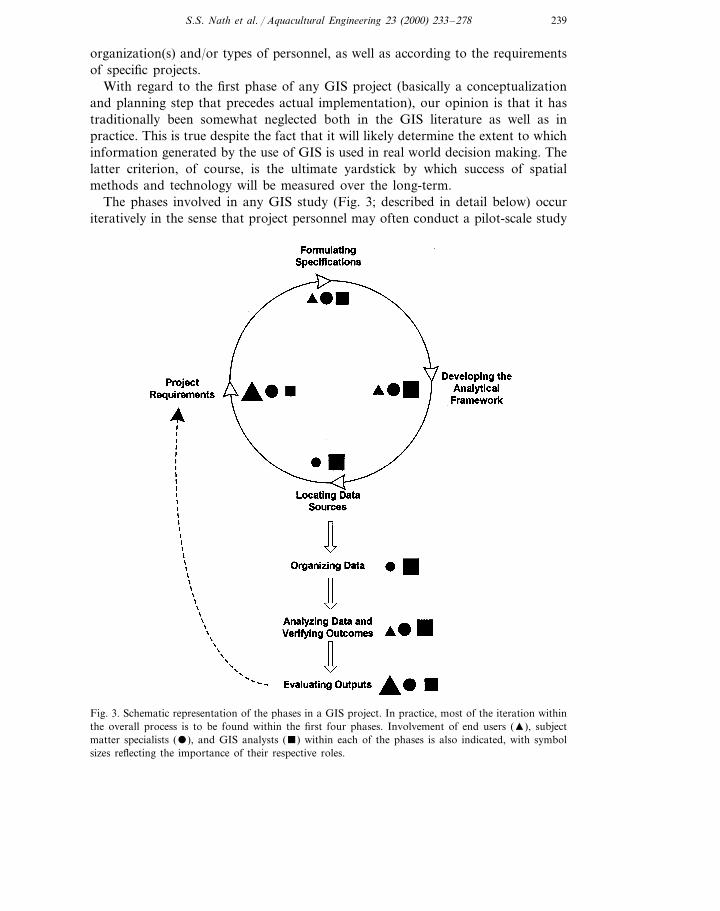
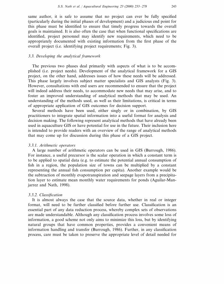
Ideally, any GIS study will consist of seven phases: identifying project require-ments, formulating specifications, developing the analytical framework, locatingdata sources, organizing and manipulating data for input, analyzing data andverifying outcomes, and evaluating outputs (Fig. 3). In practice, it may be necessaryto iterate within the overall process, particularly among the first four phases. Thefigure also indicates the degree to which different types of project personnel namelyend users, subject matter experts, and GIS analysts can be expected to be involved.The degree of personnel involvement within each phase will vary according to the
239S.S. Nath et al. / Aquacultural Engineering 23 (2000) 233–278
organization(s) and/or types of personnel, as well as according to the requirementsof specific projects.
With regard to the first phase of any GIS project (basically a conceptualizationand planning step that precedes actual implementation), our opinion is that it hastraditionally been somewhat neglected both in the GIS literature as well as inpractice. This is true despite the fact that it will likely determine the extent to whichinformation generated by the use of GIS is used in real world decision making. Thelatter criterion, of course, is the ultimate yardstick by which success of spatialmethods and technology will be measured over the long-term.
The phases involved in any GIS study (Fig. 3; described in detail below) occuriteratively in the sense that project personnel may often conduct a pilot-scale study
Fig. 3. Schematic representation of the phases in a GIS project. In practice, most of the iteration withinthe overall process is to be found within the first four phases. Involvement of end users (�), subjectmatter specialists (), and GIS analysts () within each of the phases is also indicated, with symbolsizes reflecting the importance of their respective roles.
240 S.S. Nath et al. / Aquacultural Engineering 23 (2000) 233–278
with available information, and then successively enhance and/or refine the analysisuntil a satisfactory end point is reached. Alternately, subsequent phases in theproject cycle may result in new information that needs to be incorporated in thepreceding phase(s). For example, it may become evident during the development ofthe analytical framework that requirements documented during the first iteration ofthe project cycle (Fig. 3) may need to be revised.
Recognizing the iterative nature of a GIS study allows the entire project team todevelop an improved understanding of the issue on hand, and how spatial methodsand technology can be best be used to address it. Once project personnel explicitlyrecognize that GIS work is iterative in nature and begin to document what is learntduring each phase, it becomes easier to track how user requirements are explicitlyaddressed during implementation (often referred to as traceability in the softwareliterature; Ambler, 1998), and to deliver timely as well as meaningful projectupdates (e.g. GIS outputs and reports).
3.1. Identifying project requirements
The process of identifying requirements for a GIS is essentially a multiplestakeholder decision-making situation. This is because such work is invariablyexecuted by a group of subject matter experts and analysts, and because results ofthe analyses are potentially useful to a range of decision-makers. Individuals inthese three broad groups of stakeholders are likely to have different perspectivesand expectations with regard to the capabilities and limitations of GIS. It isimportant that these perspectives and expectations are allowed to surface during theearly stages of GIS work so that an enabling environment can be created withinwhich decision support needs of end users are discussed and project goalsformulated.
Once project personnel, particularly end users, have had an opportunity topresent their spatial decision support needs, discussions can begin to examine howGIS tools can address these needs, and clarify the limitations of such tools (e.g.spatial data availability and quality, software/hardware resources that may beneeded, cost and time constraints, etc.). At this stage, it is usually not necessary oreven productive to invest an inordinate amount of time in discussing these issues.Instead, the intent is to develop common understanding about decision supportneeds, specify project goals, clarify GIS functionality and develop a listing ofgeneral requirements. More importantly, such discussions can facilitate the develop-ment of a creative and productive project team, wherein each participant has anopportunity to identify their own roles and responsibilities, and those of theirpartners.
The above observations are consistent with the work by Campbell (1994) (seealso Campbell and Masser, 1995), who suggests that the following factors areimportant in successful GIS implementation and its subsequent use in decision-making:� an information management strategy in which the needs of users are clarified,
and resources and values of the organization(s) are accounted for;
241S.S. Nath et al. / Aquacultural Engineering 23 (2000) 233–278
� identification of simple applications that generate information fundamental tothe work of potential users;
� implementation that is user-directed, and which has the commitment and partic-ipation of staff throughout the organization(s) involved; and
� the ability for the organization(s) to create sufficient stability or to be able tocope with change, both in terms of evolving specifications and rapidly changingtechnology.In our own experience, there has been a tendency among some of the technical
assistance organizations with which we collaborate to invest a considerable amountof time, effort and financial resources in developing GIS capabilities and acquiringexpensive spatial datasets. However, it is often the case that this investment is madewithout a clear understanding about what they wish to accomplish with suchcapabilities, and the stakeholder groups (both within and outside the organization)whose decision support needs they are attempting to fulfil. More often than not,GIS capabilities of such organizations are primarily used as a tool for generatingand displaying maps. The current state of spatial methods and technology, on theother hand, clearly indicates that GIS capabilities go beyond data management andvisualization alone.
For instance, process-based models and GIS (especially raster systems) are verycomplementary tools in that the former can be used to generate new output layersfrom multiple base maps already in GIS format. The derived layers often containinformation that is more useful to decision-makers. Moreover, it is now possible todirectly integrate within GIS models that have distributed (i.e. spatially explicit)parameters, and to seamlessly run alternate scenarios within a single softwarepackage. Prior to the availability of such techniques, it was necessary to executemultiple model runs outside of a GIS environment, and to import the output intoGIS for visualization. Such indirect coupling often requires additional time andtechnical expertise to handle model management and data transfer requirements,besides limiting the range of scenarios that end users may wish to analyze. Directintegration of models within GIS, however, has the potential to enable such usersin the aquaculture domain to explore alternate scenarios in a truly interactive way,simultaneously reducing the need for the continued presence of analysts or at leastusing their expertise in a manner that is more cost effective. The trend towardsinteractive GIS use is already evident in both in the business world and in somenatural resource management domains such as conservation efforts.
Another observation to be made in the current context is that if the targetdecision support audience is not adequately consulted to assess their needs, thepossibility exists that considerable effort may be expended by organizations togenerate information that is rarely used by the intended audience. The fundamentalmessage here is that if end users are involved early on in the planning process forGIS projects and their needs better understood, experts and analysts are more likelyto generate strategies that better address these needs. Moreover, they are also morelikely to make optimal use of spatial methods and technology within any organiza-tional constraints that may exist. It should be noted that our observations aboutadopting a stakeholder-driven approach to project design and management, and
242 S.S. Nath et al. / Aquacultural Engineering 23 (2000) 233–278
specific techniques to manage the process are not unique to GIS applications, butare increasingly recognized within a number of domains including organizationaldevelopment (Adams, 1986; Senge, 1990), concurrent engineering design (Voland,1992), and information technology (Ambler, 1998).
3.2. Formulating specifications
The goals and requirements of the project articulated in the first phase above areby necessity of a general nature. This is largely because it is rarely productive toembark upon an exercise to specify project components without a broad under-standing of decision support needs. Furthermore, if team members begin to focustoo much on project specifics early on in the overall process, they run the risk ofnot being able to adequately accommodate additional needs of end users (given thatsuch needs usually tend to evolve over time), and of already confining themselves toa certain mindset about implementation strategies.
However, once an overall understanding of project requirements has beendeveloped among team members, it is helpful to develop a listing of morefunctional specifications corresponding to each of the requirements that have beenidentified. For instance, if the project requires that the final GIS be interactive(implying that the end user can explore alternate scenarios on their own), one ormore of the following are representative of possible functional specifications:� capability of generating and editing different thematic maps;� features for querying attributes in spatial databases;� support for adding new themes and/or updating current information in the GIS
over time;� enabling application of the analytical approach to different geographical regions;
and� capability to modify existing models and/or link new models to the GIS.
The process of identifying functional specifications involves an in-depth analysisof each of the project requirements. In practice, it is usually beneficial for thesubject matter experts and GIS analysts to first formulate project specificationsjointly, and to then share these with the end users. This approach tends to result intime (and therefore cost) savings. Moreover, the need for communicating (poten-tially) difficult technical concepts is minimized because end users are likely to bemore interested in the actual specifications, rather than in the process by which theywere determined.
The benefits of formulating specifications for a GIS project far outweigh theinitial investment in terms of resource and time commitments. Some of the benefitsinclude an increased probability of implementing a system that does indeed meetend user needs, laying the foundation for a work breakdown structure withassociated timelines and responsibilities (for different project personnel), and animproved likelihood of building a GIS with the appropriate types of hardware andsoftware tools. Experience from the software industry also suggests that whenproject specifications are formally identified, there is an improved probability ofminimizing cost over-runs and time delays. On the other hand, as noted by the
243S.S. Nath et al. / Aquacultural Engineering 23 (2000) 233–278
same author, it is safe to assume that no project can ever be fully specified(particularly during the initial phases of development) and a judicious end point forthis phase must be identified to ensure that timely progress towards the overallgoals is maintained. It is also often the case that when functional specifications areidentified, project personnel may identify new requirements, which need to beappropriately documented with existing information from the first phase of theoverall project (i.e. identifying project requirements; Fig. 3).
3.3. De6eloping the analytical framework
The previous two phases deal primarily with aspects of what is to be accom-plished (i.e. project needs). Development of the analytical framework for a GISproject, on the other hand, addresses issues of how these needs will be addressed.This phase largely involves subject matter specialists and GIS analysts (Fig. 3).However, consultations with end users are recommended to ensure that the projectwill indeed address their needs, to accommodate new needs that may arise, and tofoster an improved understanding of analytical methods that may be used. Anunderstanding of the methods used, as well as their limitations, is critical in termsof appropriate application of GIS outcomes for decision support.
Several methods have been used, either singly or in combination, by GISpractitioners to integrate spatial information into a useful format for analysis anddecision making. The following represent analytical methods that have already beenused in aquaculture GIS or have potential for use in the future. Their inclusion hereis intended to provide readers with an overview of the range of analytical methodsthat may come up for discussion during this phase of a GIS project.
3.3.1. Arithmetic operatorsA large number of arithmetic operators can be used in GIS (Burrough, 1986).
For instance, a useful precursor is the scalar operation in which a constant term isto be applied to spatial data (e.g. to estimate the potential annual consumption offish in a region, the population size of towns can be multiplied by a constantrepresenting the annual fish consumption per capita). Another example would bethe subtraction of monthly evapotranspiration and seepage layers from a precipita-tion layer to estimate mean monthly water requirements for ponds (Aguilar-Man-jarrez and Nath, 1998).
3.3.2. ClassificationIt is almost always the case that the source data, whether in real or integer
format, will need to be further classified before further use. Classification is anessential part of any data reduction process, whereby complex sets of observationsare made understandable. Although any classification process involves some loss ofinformation, a good scheme not only aims to minimize this loss, but by identifyingnatural groups that have common properties, provides a convenient means ofinformation handling and transfer (Burrough, 1986). Further, in any classificationprocess, care must be taken to preserve the appropriate level of detail needed for
244 S.S. Nath et al. / Aquacultural Engineering 23 (2000) 233–278
sensible decision making at a later stage (Burrough, 1986; Aguilar-Manjarrez, 1996;Ross, 1998).
Aguilar-Manjarrez (1996) provides an exhaustive review of five methods thathave been explored to classify data on land types for various uses:1. The FAO land evaluation methodology which assesses land suitability in terms
of an attribute set corresponding to different activities.2. The limitation method in which each land characteristic is evaluated on a
relative scale of limitations.3. The parametric method in which limitation levels for each characteristic are
rated on a scale of 0 to 1, from which a land index (%) is calculated as theproduct of the individual rating values of all characteristics.
4. The Boolean method which assumes that all questions related to land usesuitability can be answered in a binary fashion, and that all important changesoccur at a defined class boundary.
5. The fuzzy set method in which an explicit weight is used to assess the impact ofeach land characteristic. Fuzzy techniques are then used to combine the evalua-tion of each land characteristic into a final suitability index. Apart from adominant suitability class, the fuzzy set method equally provides information onthe extent to which a certain land unit belongs to each of the suitability classesdiscerned.
For GIS applications, any of the above methods can be used to classify sourcedata into a four- or five-point scale of suitability (with one being the least suitable).However, the choice among classification methods is dependent on the type of dataand intended uses of the output information. Classification allows normalization ofall data layers, an essential pre-requisite for further modeling. An example is thegrouping of soil data into four classes based on a number of properties importantfor pond construction (Kapetsky and Nath, 1997).
3.3.3. Simple o6erlayThe most common technique in geographic information processing is that of
topological overlaying in which multiple data layers are overlain in a verticalmanner. Topological overlays may be broadly classified into simple and weighted(see below) methods. After reclassification of thematic maps in terms of suitabilityfor an activity has been accomplished, simple overlay can be accomplished byapplying mathematical or logical operators to the layers. This can often generatevery valuable outcomes. Simple overlays operations assume that all layers haveequal importance. Outcomes of the operation can be further refined if they areoverlain with constraint layers by subtraction. A more common practice, however,is to represent constraint layers in Boolean format, with disallowed and allowedareas defined as 0 and 1, respectively. In this way, when the constraint layer ismultiplied by one containing suitability data, the former is automatically excludedfrom the outcome. A series of such simple reclassifications and overlays can beassembled as a tree of sequential choices (i.e. a decision tree) to provide a rationaloutcome to a spatial problem. Examples of constraint layers are large water bodiesand forested lands that are unavailable for aquaculture (Kapetsky and Nath, 1997).
245S.S. Nath et al. / Aquacultural Engineering 23 (2000) 233–278
3.3.4. Weighted o6erlayIn decision making, it is usually the case that different attributes under consider-
ation do not have the same level of importance. This calls for a weighted overlayapproach, in which each layer is assigned a weight that is proportional to itsimportance. To accomplish this, each source layer is first reclassified onto acommon scale and then multiplied by a weighting factor. The resulting values areused in further overlay operations to obtain an outcome (applying Booleanconstraints in the final stage if needed).
The derivation of weightings for source attributes is often assumed to be anobjective scientific matter. However, it is clear from a range of studies that evenexpert opinions on ranking of attributes may differ substantially. Aguilar-Manjar-rez (1996) showed that, from a list of attributes, a group of experts with similarbackgrounds generally agree upon which are the most relevant to use for any givendecision process. However, the ranking assigned to the attributes by these expertscan differ. In general, Aguilar-Manjarrez (1996) showed that from a list of tenselected attributes, different experts would be in agreement on the priority of thefirst three to four and the last three. However, attributes with mid-level priority areoften dealt with quite differently. Moreover, subject matter experts with differentbackgrounds (e.g. aquaculturist, coastal zone planner, conservationist, etc.) bringdiffering agendas to the same problem, resulting in a range of outcomes. At worst,it is clear that without guidance, a range of prioritizations can be obtained whichare cumulatively meaningless. GIS analysts therefore need to ensure that weightingsapplied personally are as objective as possible and that where expert group input isused, the basis for this input is fully explained and carefully analyzed before its usefor decision making. Summary tables that transparently document factors used inthe evaluation and the weights assigned to them by different experts are a useful aidin this regard (Aguilar-Manjarrez, 1996; Aguilar-Manjarrez and Nath, 1998).
As the number of layers in a model increases, the logic of processing them canbecome confusing. Consequently, special routines to assist with this process havebeen provided in certain GIS packages. For example, the decision support modulein IDRISI (Eastman, 1993) supports multi-criteria evaluation (MCE), which isbased on the analytical hierarchy process (AHP) described by Saaty (1980). Thismodule enables a structured, logical approach to weighted overlay with built-incrosschecks at some stages of the weighting process to ensure consistency of logicby the operator. AHP falls into the broader category of pairwise comparisontechniques in which attributes are ranked against each other to assess their relativeimportance. Although AHP or other pairwise comparison variants do provideopportunity for increased objectivity in the ranking of factors, they do notadequately address the issue of different weightings that may be assigned by diversesubject matter experts. For instance, different weightings were assigned to factorsimportant for pond aquaculture by different experts in continental-scale GISstudies (Kapetsky and Nath, 1997; Aguilar-Manjarrez and Nath, 1998). The AHPprocess was useful in these studies in terms of providing a logical framework forcomparing the factors. However, in both instances, the authors ultimately relied ontheir own ranking schemes (which had similar patterns to those of the experts) to
246 S.S. Nath et al. / Aquacultural Engineering 23 (2000) 233–278
assign weights to the factors. In general, it is unlikely that technical methods suchas AHP or other multi-criteria decision making tools (see review by Merkhofer,1998) can be a complete replacement to a well-facilitated exercise in whichstakeholders (i.e. subject matter specialists, GIS analysts and end users in thecurrent context) are encouraged to seek consensus on the relative importance ofattributes for use in GIS. Instead, such tools should be viewed as providingadditional support to the consensus building process.
3.3.5. Neighborhood analysisA key function provided by GIS, and one which cannot be easily addressed by
the use of any other decision support tool, is its capability to allow evaluation ofthe characteristics of an area that surrounds a specific location, which is referred toas neighborhood analysis. GIS software provides a range of neighborhood func-tions including point interpolation techniques in which unknown values are esti-mated from known values of neighboring locations. These techniques are typicallyused to convert point coverages into grids or to generate elevation data either intriangular irregular network (TIN) format for vector GIS or as a digital elevationmodel (DEM) for raster GIS. DEMs have not as yet found widespread use inaquaculture, but are often at the heart of environmental GIS that are targetedtowards analyses of entire landscapes. For instance, the DEM for a watershed ofinterest is a key layer in many spatially explicit hydrological models. In the future,such tools are likely to find applications in aquaculture from the perspectives ofassessing water availability and modeling environmental impacts of existing and/orproposed aquaculture operations. A common type of neighborhood operation isbuffering, which allows the creation of distance buffers (or buffer zones) aroundselected features. An example where this operation may be useful in aquaculture iswhen there is a need to determine how many streams are available (or to beavoided) within a specified distance of a proposed facility.
3.3.6. Connecti6ity analysisThis type of analysis is characterized by an accumulation of values over the area
that is being traversed. Support for connectivity analysis in commercially availableGIS software is not as standardized in comparison to the operators describedabove. Network analysis is one type of connectivity operation, which is character-ized by the use of feature networks such as hydrographic hierarchies (i.e. streamnetworks) and transportation networks. As an example of the use of networkanalysis in aquaculture, Kapetsky and Nath (1997) estimated the shortest trans-portation path from a given site to the nearest market.
The most sophisticated type of connectivity operation is three dimensionalanalysis which is helpful in terms of visualizing impacts of alternate decisions onentire landscapes (e.g. watersheds). Such advanced features of GIS are likely tohave applications in aquaculture but have apparently yet to be used in the systemsthat have been developed in this domain.
247S.S. Nath et al. / Aquacultural Engineering 23 (2000) 233–278
3.3.7. Hierarchical modelsIn practice, comprehensive representation of the real world in a GIS often
involves the use of a large number of source variables, which when processed intoGIS using one or more of the analytical methods described above, may result inconsiderable complexity. Experience suggests that when the number of layersexceeds about 10, MCE becomes difficult, even to the experienced modeler. Suchsituations warrant the development of a hierarchical modeling scheme.
In this approach, naturally grouped variables are first considered together toproduce ‘sub-model’ outcomes such as water needs, soil suitability, input availabil-ity, farm gate sales, and markets (Kapetsky and Nath, 1997). It is often the casethat a source variable or processed layer will be used in more than one sub-modeland that the layer may need to be transformed depending on the intended purpose.Each of these sub-models may, in turn, be derived from lower-level models whichpre-process variable data into useful factors. Another example from aquaculture isthe estimation of wave height from wind velocity and fetch (Ross et al., 1993).
It is, of course, not necessary to embed all of the models and/or sub-modelswithin a single system per se. This is because commercial GIS can export andimport information quite seamlessly with external modules. For instance, growthestimates derived from an external bioenergetic model (linked to spatial weatherand water temperature datasets) have been used to predict fish yields in continental-scale GIS (Kapetsky and Nath, 1997; Aguilar-Manjarrez and Nath, 1998). In adifferent context, external rule-based systems are being used in conjunction withGIS to generate future agricultural land use patterns for assessing policy alterna-tives in the Pacific Northwest region of the United States (Bolte, unpublishedinformation).
3.3.8. Multi-objecti6e land allocationOnce an activity has been modeled and quantified, it will invariably have some
potential to conflict with other uses of the space or resources. For example,practices such as agriculture, forestry, and aquaculture may compete for availableland and associated resources. This calls for trade-off decisions to be made so thatactivities can coexist. These decisions typically require consideration of economic,environmental and social ramifications of alternative land use practices. Decisionsupport tools are available in some GIS packages to facilitate this process. Themulti-objective land allocation (MOLA) and multi-dimensional decision space(MDCHOICE) tools in IDRISI are good examples. MOLA was used by Aguilar-Manjarrez and Ross (1995) to identify areas suitable for agriculture and aquacul-ture across the Sinaloa state of Mexico (see section on case studies below). Inputsfor the MOLA technique originate from the results of weighted overlays. Theapproach allows GIS analysts to set limits on areas required for different land usesand assign requirements for these uses. An iterative process is then used tosuccessively reassign ranked cells to alternate activities depending upon how closelythey match the associated requirements.
248 S.S. Nath et al. / Aquacultural Engineering 23 (2000) 233–278
3.4. Identifying data sources
Once the analytical framework has been developed, it is necessary to identifydata sources to be used in the project. This phase is largely restricted to GISanalysts (Fig. 3), although subject matter specialists often provide helpful advice(e.g. identifying non-spatial datasets). Information for spatial decision-making andanalysis is varied, and will usually consist of data describing the biophysical,economic, social and infrastructural environments. These data can come from avariety of sources ranging from primary data gathered in the field or satellite scenesto all forms of secondary data, including textual databases and reports.
It is generally both costly and time consuming to collect field (primary) data firsthand. Therefore, all GIS practitioners attempt to locate the data they need fromexisting secondary sources, either in paper or digital form. The initial considerationis identifying what data are needed for the overall analysis. This is followed byattempts to source the data, and to assess their age, scale, quality and relative cost.Different data types are often developed in different geographic coordinate systems,and must be re-projected onto a common coordinate system. Other common issuesare ensuring that features common across multiple layers are spatially coincident,and understanding the resolution, constraints and uncertainty associated with thedata. For these reasons, data collection and preprocessing are typically the mostexpensive and time-consuming component of an analysis.
Digital database availability is increasing at a rapid rate throughout the world.These databases contain information ranging from natural resources (e.g. maps ofsoils, water resources and temperature distributions), to population census andcadastral (i.e. property ownership and associated boundaries) data. In many cases,such data may only be available in hard copy reports, although information is alsoavailable on CD-ROMs, from which databases for GIS use can be extracted.
A further source of data is the WWW, from which a wide range of mapped andother spatial data can be found by carefully executed searches. Spatial informationat low resolution can often be obtained in this way, good examples being theGlobal 30 arc second elevation (http://edcwww.cr.usgs.gov/landdaac/gtopo30/gtopo30.html), and the 1-km Global Land Cover datasets. Other online datasetsinclude information on drainage basins, and weather, which can be downloadedfrom Web sites at some universities and international agencies. In this regard, auseful site that provides metadata search capabilities and access to a range of dataresources is the one maintained by the Center for International Earth ScienceInformation Network (CIESIN) at http://www.ciesin.org. In some countries such asthe USA, GIS clearinghouses have been established on the Web and offer access toconsolidated datasets from multiple agencies (see http://www.usgs.gov). Many ofthese free spatial databases are of immense value and should not be overlooked.
The ‘lingua franca’ of GIS is the thematic map in which particular attributes ofthe geographical region are represented digitally or on a specially prepared hardcopy map. Clearly, where such maps are available in digital form, they are directlyusable in a GIS. Hard copy maps can also be digitized, and the informationimported into GIS. The digitizing process, however, is very time consuming andrequires many hours of data editing to ensure superior quality.
249S.S. Nath et al. / Aquacultural Engineering 23 (2000) 233–278
Thematic data can be in the form of a choropleth (areas of equal value separatedby boundaries), isopleth (lines which connect points of equal value) or point maps(Burrough, 1986), all of which are often valuable, a good example in terms ofaquaculture being the hydrographic chart. The more common topographic mapfrequently contains many thematic data (including elevations, water bodies, roads,cities, and woodlands) which are of value to the GIS analyst. These themes can beextracted at the stage of digitization, and established as separate layers in thespatial database.
3.5. Organizing and manipulating data
After datasets have been collected, it is necessary to organize and manipulatethem for use in the target GIS. This phase is also largely restricted to GIS analysts(Fig. 3), although depending on the type of application, occasional interaction withsubject matter specialists may be warranted. Some of the key activities that occurin this phase include verification of data quality, data consolidation and reformat-ting, creation of proxy data and database construction. Proxy data refer toinformation that is derived from another data source, for which establishedrelationships may exist. Examples include estimation of water temperature from airtemperature (Kapetsky, 1994), extraction of semi-quantitative texture from FAOsoil distribution maps (Kapetsky and Nath, 1997) or calculation of maximum waveheights from wind speed and fetch (Ross et al., 1993).
In terms of verification of data quality, the reliability of thematic maps world-wide is variable, as is the currency of their content. These aspects must beconsidered where critical decisions are based upon such material. Although digitalmaps are often quite up to date, the spatial accuracy of some printed material canbe suspect. Critical assessment and verification of source data quality is veryimportant. The value of such verification for all input data cannot be over-stressed,before digitizing as well as after the fact. It is usually the case that at least some ofthe layers required in a GIS database will not be of a high enough standard, andverification on paper may very well need to become verification by survey, wherewarranted. A detailed overview of technical methods to address data quality issuesis available in Burrough (1986).
Certain data sources such as satellite data are already in digital form, but allothers may require some work in order to consolidate them for spatial analysis.Satellite images provide a rich source of data in a form suitable for use in a spatialdatabase. The information collected by the scanners on LANDSAT and SPOT areaimed specifically at natural resource work and the source data can be reprocessedin a variety of ways to reveal details of the environment that may not be apparentin the raw state.
Most GIS packages have tools to assist with reprocessing, including the ability tofilter and clean up the image, make corrections for atmospheric variations andallow georeferencing of the image to known reference points (Burrough, 1986).Images can then be classified based on spectral signatures of different features ofthe environment such as forest, grassland, and water bodies so as to reveal different
250 S.S. Nath et al. / Aquacultural Engineering 23 (2000) 233–278
land uses, often in some detail. A number of widely used vegetation indices, suchas normalized difference vegetation index (NDVI), can also be calculated and theresultant thematic data extracted for immediate use in GIS. A potential example inaquaculture would be the development of an algal bloom index to assess the risk offish kills due to dissolved oxygen depletion in pond systems. The digital nature ofthe product means that the data are easy to incorporate and their relative costs lowcompared to primary data collection surveys. Remotely sensed images are thereforea common starting point for GIS work.
Reformatting of data for use in a particular GIS may also include classificationof the information (as discussed in the preceding section on analytical methods) andconversion of available data from vector to raster format (or vice versa). Finally,spatial data are often available at different resolutions, and it is necessary toconvert the datasets to the desired scale for the analysis to ensure appropriate dataprocessing. This may very well involve seeking expert opinion on the validity ofreconciling scale differences.
Database construction is another set of activities that is typically undertaken inthis phase. Designing an appropriate database is important both in terms ofensuring that the information can be readily accessed for the target application, andis available for re-use at a later time. It has been the case in the past that spatialdata were usually stored in formats suited to the type of GIS software being used.This often resulted in spatial databases that were not relatively easy to extract eitherfor use in other types of applications or software. However, many organizations aretaking advantage of recent advances both in GIS and database technology bystoring both raw and processed information in relational databases. Such data canseamlessly be imported for use in stand-alone GIS applications, but are in principleavailable for alternate uses (e.g. data publishing across the WWW).
3.6. Analyzing data and 6erifying outcomes
This phase represents the culmination of effort that has been expended, particu-larly on the part of GIS analysts, to develop the analytical framework, locate datasources and organize data for the analysis. As can be expected, the GIS analystsplay the most important role in this phase but are likely to interact with subjectmatter specialists and end users in terms of verifying preliminary results (Fig. 3).Activities that may be encountered in this phase include executing analyticalmethods (i.e. overlays, model runs and/or other querying knowledge based systems,etc.), importing and exporting data as needed (e.g. intermediate GIS outputs whichare required by other components within the overall analytical framework), compu-tation of relevant statistics (e.g. means, standard deviations, ranges, classes, etc.),generation of output information (e.g. maps, tables, graphs, and reports), andverification of outcomes.
Field verification as part of any GIS work is absolutely essential, both for qualitycontrol of certain data sources (as previously discussed) and for testing theoutcomes of models (or other analytical tools). Although environments and activi-ties can be modeled in total isolation as an academic exercise, it is only throughcareful verification that the general applicability of results can be ensured.
251S.S. Nath et al. / Aquacultural Engineering 23 (2000) 233–278
Fieldwork as part of a verification exercise is frequently referred to as ground-truthing. The general approach to such work is similar to any field survey, andstandard techniques for survey, and environmental measurements can be used. Themain difference is in the sampling plan and a verification exercise will typically bebased on a series of sample points designed to cover the area. Such coverages wouldnormally be well distributed over the ground or water surface, but are often moreefficient if a random stratified sampling pattern is used. This allows effort to beconcentrated on ensuring that differences between different features in the land-scape are assessed, rather than using a simple randomized pattern, which mayrepeatedly cover a large uniform area.
Global positioning systems (GPS) have greatly aided the spatial accuracy ofground-truthing and field verification, in most cases removing the need to usesurveying techniques completely. These systems provide three-dimensional positionlocations from satellites to within about 100 m under normal operation, althoughactual accuracy is frequently as good as 20 m or even less. By operating indifferential mode, two GPS units can give real-time locations accurate to less thana meter and with post-processing to within a few millimeters (Aguilar-Manjarrez,1996). The value of these systems has been rapidly recognized by GIS practitioners.Some GIS data acquisition systems will accept direct input from GPS so that thelocation can be displayed over a real satellite image of the study area.
Apart verifying data and outcomes of models, field verification can providefeedback into the analytical process itself by allowing the GIS analysts and subjectmatter specialists to understand, quantify and document errors of the assumptionsused. Such documentation should be an integral part of the overall project report.
3.7. E6aluating outputs
In this final phase of a GIS project, outputs generated are jointly evaluated bythe overall team (i.e. end users, subject matter specialists and analysts; Fig. 3).Several activities are likely to be encountered during this phase, including asummary review of key findings, more detailed examination of individual compo-nents of the project together with their underlying assumptions, limitations (if any)of the findings, and an evaluation of the degree to which each of the originalrequirements of the project have been met. The results of the latter activity providea useful means of assessing the success of the project. However, it is often the casethat outputs from a GIS project are not put to immediate use, but form acomponent of a larger decision making process (e.g. development of new policiesand/or development plans pertaining to). In this regard, it may be difficult toproperly assess the value of the information generated by a GIS project, andtherefore its contribution towards decision support. If careful attention is given tothis aspect at the beginning of a GIS project (i.e. during the phase of identifyingproject requirements), it should be possible to develop a set of indicators which canbe measured over time and used to track how GIS information is used inaquaculture decision making by end users. Feedback from such indicators is likelyto be helpful in improving further GIS development and application.
252 S.S. Nath et al. / Aquacultural Engineering 23 (2000) 233–278
Little work has apparently been done in the area of indicator monitoring bypersonnel involved in aquaculture GIS, perhaps because many of the efforts to datehave been undertaken primarily as academic exercises. In other contexts where GIShave been developed by technical assistance organizations, it would appear that animplicit assumption by the implementing personnel is that if the information isproduced, the target audience of decision makers would actually use it. However,because end users have often not been consulted in aquaculture GIS projects (aspreviously indicated), this assumption is somewhat questionable. Clearly, there isneed for typical end users, subject matter specialists and spatial analysts tocollaborate more actively in the development and application of GIS foraquaculture.
4. Case studies in aquaculture
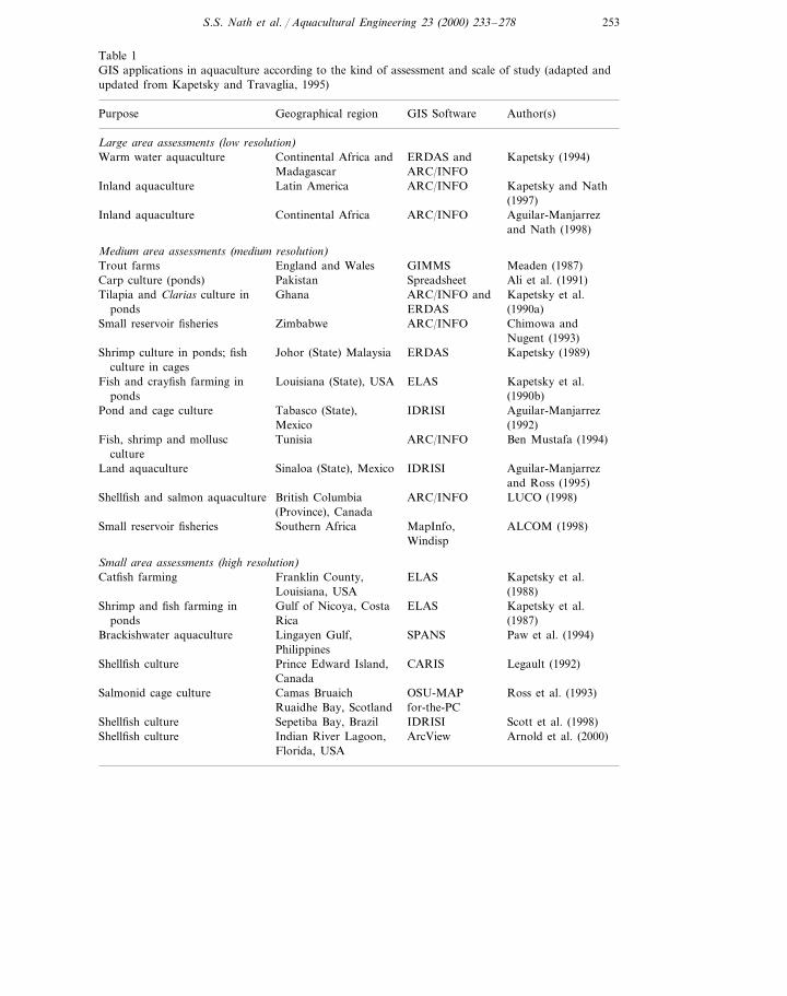
The use of GIS in aquaculture, together with selected cases, has previously beendocumented (Meaden and Kapetsky, 1991; Kapetsky and Travaglia, 1995; Aguilar-Manjarrez, 1996; Ross, 1998). In this section, we build on the foundation that hasbeen set forth by the above authors, specifically examining selected cases (in somedetail) from the perspective of their applications for spatial decision support inaquaculture. A more comprehensive listing of GIS applications for aquaculture ispresented in Table 1 (see Meaden and Kapetsky, 1991 and Aguilar-Manjarrez, 1996for other examples).
The selected cases represent a broad sampling across geographic scales rangingfrom local areas (i.e. a small bay), to sub-national regions (i.e. individual states/provinces), to national and continental expanses. They also vary with regard to thedegree to which GIS outcomes have been used for practical decision making.Further, the case studies demonstrate the large extent of GIS applications that arepossible in aquaculture including: site selection for targeted species, environmentalimpact assessment, conflicts and trade-offs among alternate uses of natural re-sources, and consideration of the potential for aquaculture from the perspectives oftechnical assistance and alleviation of food security. The cases also vary signifi-cantly with regard to complexity of the analytical methods used (i.e. ranging fromsimple overlays to weighted combinations to use of relatively sophisticated models).Finally, the case studies are indicative of issues associated with data procurementand manipulation, and the diversity of GIS packages that are available. Each of thecase studies is presented in the following format:� source of the work;� objectives;� target decision support audience;� geographic area and scale of analysis;� analytical methods and results; and� comments (e.g. limitations of the approaches used, possible enhancements, and
actual use for decision making).
253S.S. Nath et al. / Aquacultural Engineering 23 (2000) 233–278
Table 1GIS applications in aquaculture according to the kind of assessment and scale of study (adapted andupdated from Kapetsky and Travaglia, 1995)
Author(s)GIS SoftwarePurpose Geographical region
Large area assessments (low resolution)Warm water aquaculture Continental Africa and ERDAS and Kapetsky (1994)
Madagascar ARC/INFOInland aquaculture Kapetsky and NathLatin America ARC/INFO
(1997)Inland aquaculture ARC/INFO Aguilar-ManjarrezContinental Africa
and Nath (1998)
Medium area assessments (medium resolution)Meaden (1987)GIMMSEngland and WalesTrout farmsAli et al. (1991)Carp culture (ponds) Pakistan Spreadsheet
ARC/INFO andGhana Kapetsky et al.Tilapia and Clarias culture in(1990a)ERDASponds
ARC/INFOZimbabwe Chimowa andSmall reservoir fisheriesNugent (1993)
ERDASJohor (State) Malaysia Kapetsky (1989)Shrimp culture in ponds; fishculture in cages
Louisiana (State), USAFish and crayfish farming in ELAS Kapetsky et al.(1990b)ponds
IDRISIPond and cage culture Aguilar-ManjarrezTabasco (State),Mexico (1992)
ARC/INFOFish, shrimp and mollusc Ben Mustafa (1994)Tunisiaculture
Sinaloa (State), Mexico IDRISI Aguilar-ManjarrezLand aquacultureand Ross (1995)
ARC/INFO LUCO (1998)British ColumbiaShellfish and salmon aquaculture(Province), Canada
MapInfo,Southern AfricaSmall reservoir fisheries ALCOM (1998)Windisp
Small area assessments (high resolution)ELAS Kapetsky et al.Franklin County,Catfish farming
(1988)Louisiana, USAShrimp and fish farming in ELAS Kapetsky et al.Gulf of Nicoya, Costa
Ricaponds (1987)SPANS Paw et al. (1994)Lingayen Gulf,Brackishwater aquaculture
PhilippinesCARIS Legault (1992)Shellfish culture Prince Edward Island,
CanadaOSU-MAPCamas Bruaich Ross et al. (1993)Salmonid cage culture
Ruaidhe Bay, Scotland for-the-PCShellfish culture IDRISI Scott et al. (1998)Sepetiba Bay, Brazil
ArcView Arnold et al. (2000)Indian River Lagoon,Shellfish cultureFlorida, USA
254 S.S. Nath et al. / Aquacultural Engineering 23 (2000) 233–278
4.1. Site selection for salmonid aquaculture, Scotland (source: Ross et al., 1993)
4.1.1. Objecti6esThe primary objective of this work was to examine GIS as a tool for assessing the
potential of salmonid cage aquaculture in a small bay. A secondary objective wasto develop a general methodology for spatial analysis of coastal cage aquaculturepotential.
4.1.2. Target decision support audienceA specific audience for this work was not identified by the authors perhaps
because the work was primarily a research effort to investigate the feasibility ofusing GIS for assessing cage culture potential at a local scale (i.e. fine resolution).Nevertheless, the outcomes of the study and the GIS per se would certainly be ofinterest to governmental agencies responsible for promoting and/or monitoringaquaculture development in the bay, and to individual investors wishing to identifysuitable sites for cage culture.
4.1.3. Geographic area and scale of analysisThe study area comprised the Camas Bruaich Ruaidhe Bay located along the
West Coast of Scotland. The bay is only 19.8 ha in size. Two scales of resolution(25×25 m, and 10×10 m) were pursued in the study, of which the coarser scalewas found to be unsatisfactory for processing of most data. As noted by theauthors, however, the issue of scale is typically a trade-off between data needs/availability and objectives of the GIS work. In this case, the finer resolution wasmore appropriate.
4.1.4. Analytical methods and resultsThis study used a successive screening process for different criteria identified to
be of importance in evaluating aquaculture sites, and application of simple overlaytechniques within a very low cost raster GIS (OSU-MAP for the PC). The criteriaincluded depth, current velocity, salinity, dissolved oxygen, and temperature (con-sidered to be key factors in salmonid cage culture), as well as other factors (i.e. localinfrastructure, topography and exposure). With the exception of local infrastructure(judged to be quite suitable for aquaculture based on a qualitative assessment ofaccessibility to markets, and availability of labor, services and supplies), all of theother criteria were analyzed spatially for the entire bay.
Water quality sampling in the bay suggested that dissolved oxygen and tempera-ture were not likely to limit salmonid culture. Consequently, these two criteria wereexcluded from further analysis. Topographical information was used primarily tooutline the bay and its main features (i.e. it did not have any direct relevance to theissue of suitability for salmonid cage culture, but provided the geographical baseover which the remaining criteria were added). From a procedural perspective,following initial examination and screening of the digitized data, the criteriaultimately analyzed within the GIS were: depth (determined on the basis of abathymetric contour map), exposure (expressed in terms of a proxy variable,namely wave height), current intensity, and salinity, in that order.
255S.S. Nath et al. / Aquacultural Engineering 23 (2000) 233–278
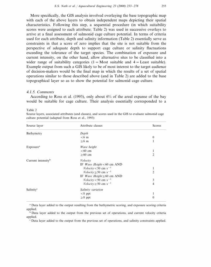
More specifically, the GIS analysis involved overlaying the base topographic mapwith each of the above layers to obtain independent maps depicting their spatialcharacteristics. Following this step, a sequential procedure (in which suitabilityscores were assigned to each attribute; Table 2) was used in successive overlays toarrive at a final assessment of salmonid cage culture potential. In terms of criteriaused for each attribute, depth and salinity information (Table 2) essentially serve asconstraints in that a score of zero implies that the site is not suitable from theperspective of adequate depth to support cage culture or salinity fluctuationsexceeding the tolerance of the target species. The combination of exposure andcurrent intensity, on the other hand, allow alternative sites to be classified into awider range of suitability categories (1=Most suitable and 4=Least suitable).Example output from such a GIS likely to be of most interest to the target audienceof decision-makers would be the final map in which the results of a set of spatialoperations similar to those described above (and in Table 2) are added to the basetopographical layer so as to show the potential for salmonid cage culture.
4.1.5. CommentsAccording to Ross et al. (1993), only about 6% of the areal expanse of the bay
would be suitable for cage culture. Their analysis essentially corresponded to a
Table 2Source layers, associated attributes (and classes), and scores used in the GIS to evaluate salmonid cageculture potential (adapted from Ross et al., 1993)
ScoresSource layer Attribute classes
Bathymetry Depth0B6 m
]6 m 1
Exposurea Wa6e heightB60 cm 1]60 cm 2
Current intensityb VelocityIF Wa6e HeightB60 cm AND
VelocityB50 cm s−1 12Velocity]50 cm s−1
IF Wa6e Height]60 cm ANDVelocityB50 cm s−1 3Velocity]50 cm s−1 4
Salinity 6ariationSalinityc
B8 ppt 1]8 ppt 0
a Data layer added to the output resulting from the bathymetric scoring, and exposure scoring criteriaapplied.
b Data layer added to the output from the previous set of operations, and current velocity criteriaapplied.
c Data layer added to the output from the previous set of operations, and salinity constraints applied.
256 S.S. Nath et al. / Aquacultural Engineering 23 (2000) 233–278
situation of ‘worst-case modelling’ in that wave heights, for instance, were com-puted based on the longest recorded fetches and highest wind speed combina-tions. In other words, the possibility exists that a larger area of the bay would besuitable for cage culture. Apart from the data used in GIS analyses of thisnature, the ‘sequence’ in which spatial operators are used will influence theoutput (Burrough, 1986; Ross et al., 1993). Thus, if the original decision se-quence (i.e. depth, exposure, current intensity, and salinity) is changed, theensuing output will be different because of Boolean algebraic operations. It istherefore important that analysts involved with GIS work closely with subjectmatter experts to establish the priority of different criteria, which in turn estab-lishes the sequence of spatial operations.
This case study is indicative of the potential advantages associated with GISuse for site selection over manual evaluation — the authors in fact made acomparison of time and resource requirements between GIS use and physicalassessment by aquaculturists. They concluded that in terms of time, the GIS wasmore efficient. However, it was more costly to conduct the GIS work,as opposed to a manual assessment — on the other hand, these costs areexpected to decline substantially as the tools and techniques are used for addi-tional projects. Moreover, if the GIS were to be refined for use in routinemonitoring (e.g. pollution assessment of the bay due to cage culture), its benefitsas a management tool would clearly outweigh the investments over the longterm. Finally, Ross et al. (1993) proposed a set of guidelines whereby a genericGIS logic sequence could be used for site selection in coastal waters. Theguidelines involve screening out locations where depths are unsuitable, gradingareas that do have adequate depth on the basis of wave heights (simultaneouslyaddressing engineering specifications for the possible types of cages), gradingthe resulting areas according to the range of current velocities, and finallyexamining water quality parameters in terms of their suitability for the targetculture species (in the geographic location where their work was conducted,oxygen and temperature were not limiting factors but may very well be in otherplaces).
It should, however, be pointed out that the guidelines proposed by Ross et al.(1993) relate only to the biophysical characteristics to be considered in siteselection for coastal areas. A more robust site selection strategy would alsoinclude detailed analysis of economic (e.g. infrastructure support, availability ofand distance to markets, etc.) and social factors (e.g. impacts on coastal commu-nities). Their implementation of a GIS for the Camas Bruaich Ruaidhe Bay didqualitatively addressed some of these factors but not in a rigorous manner. Thecase studies that follow demonstrate, to different extents, how GIS can be usedto address biophysical, economic and social factors although it should be notedthat they were designed to generate information for decision support at a morestrategic level. At the fine resolution used by Ross et al. (1993), consideration ofeconomic and social factors would, by necessity, have to include information anddata types that are very site specific.
257S.S. Nath et al. / Aquacultural Engineering 23 (2000) 233–278
4.2. Assessment of land suitability for aquaculture and agriculture in Sinaloa State,Mexico (sources: Aguilar-Manjarrez and Ross, 1995; Aguilar-Manjarrez, 1996)
4.2.1. Objecti6esThe main objective of this work was to develop a detailed GIS that could serve
as an analytical and predictive tool to guide (shrimp) aquaculture development ata state-level in Mexico. The GIS was intended to provide planners and managerswith a tool to assess land suitability for aquaculture and agriculture in the state ofSinaloa, and to provide guidance for exploring the consequence of land usedecisions before they are committed to action. Aguilar-Manjarrez (1996) alsoextended the GIS to allow evaluation of shrimp aquaculture opportunities at anindividual ‘site’ (the Huizache Caimanero Lagoon in Sinaloa). This work is notdiscussed here due to space constraints.
4.2.2. Target decision support audienceThe GIS developed by the authors (as well as outcomes generated) would be of
interest to governmental agencies responsible for promoting and/or monitoringshrimp aquaculture development in the Sinaloa State of Mexico. More likely thannot, information generated would be useful for decision making at the state,regional and national levels. Investors keen on large-scale operations would also beinterested in identifying opportunities for shrimp culture where the potential forproduction is high, and conflicts with agricultural use of the land likely to belimited.
4.2.3. Geographic area and scale of analysisThe study area comprised the zone between 22° 12%–27° 13% N and 105° 19%–109°
33% W ensuring coverage of the entire state of Sinaloa (located along Mexico’snorthwest coastline), areas of neighboring states (Sonora, Chihuahua, Durango,and Nayarit) and the Gulf of California. The authors report the area of the Sinaloastate to be roughly 58 480 km2. Spatial analysis was conducted at a resolution of250 m.
4.2.4. Analytical methods and resultsIn this study, models addressing themes pertaining to land use/environmental
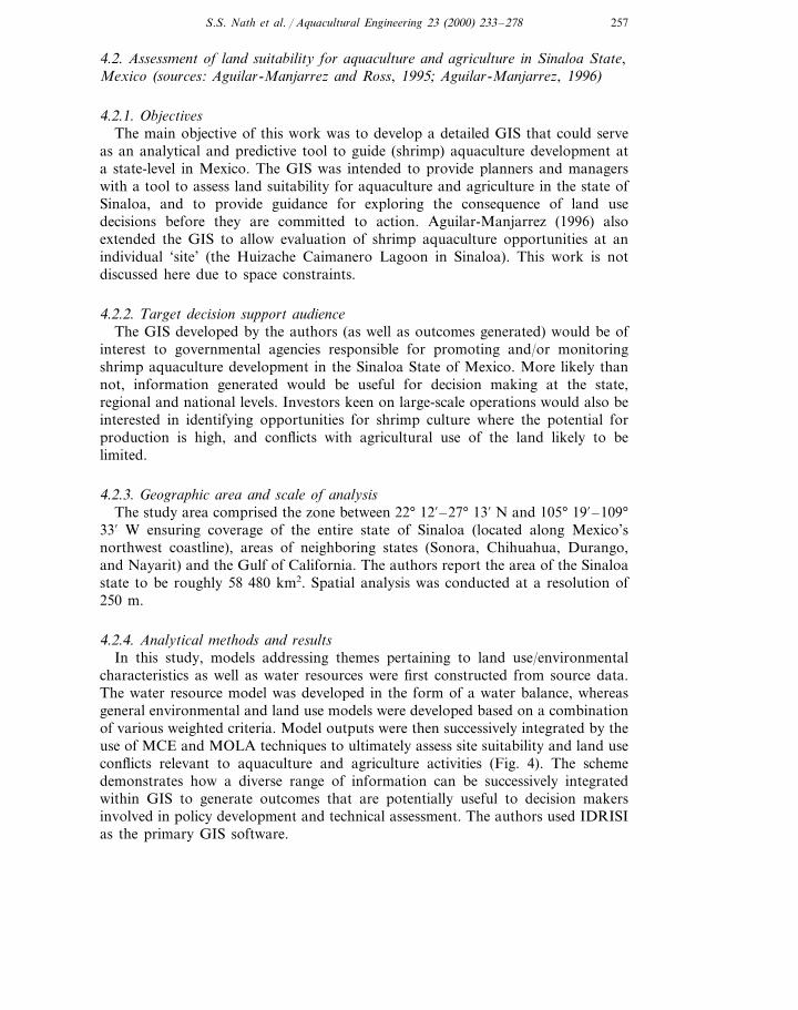
characteristics as well as water resources were first constructed from source data.The water resource model was developed in the form of a water balance, whereasgeneral environmental and land use models were developed based on a combinationof various weighted criteria. Model outputs were then successively integrated by theuse of MCE and MOLA techniques to ultimately assess site suitability and land useconflicts relevant to aquaculture and agriculture activities (Fig. 4). The schemedemonstrates how a diverse range of information can be successively integratedwithin GIS to generate outcomes that are potentially useful to decision makersinvolved in policy development and technical assessment. The authors used IDRISIas the primary GIS software.
258 S.S. Nath et al. / Aquacultural Engineering 23 (2000) 233–278
Fig. 4. A hierarchical modeling scheme with MCE and MOLA to evaluate suitability of locations foraquaculture and agriculture and resolve associated conflicts, in the Sinaloa state of Mexico (adaptedfrom Aguilar-Manjarrez and Ross, 1995).
Thirty base layers (thematic maps) were used in the study and included informa-tion ranging from pollution sources, population density, general environmentalcharacteristics, land use practices, infrastructure, and water resources (Fig. 4).These layers were organized into 14 criteria, represented either as factors (a measureof the suitability of the criterion relative to the activity under consideration) orconstraints (which limits the alternatives under consideration in a binary manner).Two broad categories of factors were identified: physical and environmentalcharacteristics (e.g. water resources, climate, temperature, soils, topography, etc.)and land use type and infrastructure (e.g. agriculture, livestock rearing, populationcenters, industries, roads, etc.). Constraints used for agriculture and aquaculturewere assumed to be identical (e.g. both activities would not be possible in protectedland and polluted areas). The identified factors were then grouped into suitabilityclasses. In this study (Aguilar-Manjarrez, 1996), it was found that the FAO,Boolean and fuzzy methods were needed to evaluate land suitability. The FAOclassification method was appropriate for factors that needed a limited threshold(such as water bodies) and Boolean classification was used when a constraint wasincorporated in the evaluation (e.g. protecting existing conservation areas likemangroves). Finally, fuzzy classification proved most appropriate for factors whoseboundaries were difficult to define, such as soils and slopes.
259S.S. Nath et al. / Aquacultural Engineering 23 (2000) 233–278
After suitability classes were assigned, the factors were weighted by the use of theAHP technique. This was followed by generation of factor maps, which in turn weremultiplied by the various constraints to mask out unsuitable areas. The process ofclassifying factors, their weighting, generation of maps, and application of con-straints involved the use of an automated MCE procedure in IDRISI.
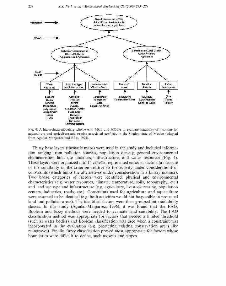
The final step in the analysis was to apply the MOLA technique in order tomaximize the land allocation area for aquaculture and agriculture. The rationalebehind the use of this technique was that aquaculture and agriculture are often inconflict because they require similar types of infrastructure, share a number ofcommon biophysical requirements, and have parallel economic and social impacts.Use of the MOLA technique requires assignment of weights for each of thealternative activities under consideration — for this study, equal weights wereassigned for aquaculture and agriculture. Outcomes of the various steps listed above(see also Fig. 4) included suitability maps for both aquaculture and agriculture, anda single map depicting areas found by the MOLA technique to be most suitable forthese two land use activities (Fig. 5).
The GIS analysis and predictions in this study were entirely dependent on a varietyof information sources (which themselves are likely to have some level of inaccuracy)and even different scales. Hence, it was considered to be of paramount importanceto carry out field verification. Moreover, it was also considered to be very importantto locate other data (e.g. pollution sources or other relevant information) which wereeither not identified or required updating during the creation of the original database.This involved the use of GPS (see Aguilar-Manjarrez, 1996 for full details) to locatepoints on the ground, and comparison of GIS output to results of a manual surveyconducted by two Mexican consultancy firms. The verification exercise suggested thatalthough the areal expanses suitable for aquaculture were comparable between theGIS and manual survey results (roughly 2090 km2 or about 3.5% of the area ofSinaloa), suitable locations that were identified differed among the two methods. Thiswas presumably because of differences in the logic and analytical techniques used.However, it would appear that outcomes from the GIS were more indicative of thetrue potential for aquaculture because of the range of criteria considered and theirintegration into suitability models. Moreover, the GIS was able to identify andresolve areas of potential conflict between agriculture and aquaculture. In principle,such information can be helpful to decision makers in terms of exploring alternativeland use practices ‘prior’ to committing them to the landscape.
4.2.5. CommentsThis case study is truly indicative of the potential for use of GIS output to evaluate
aquaculture potential and guide its development at a regional scale, particularly interms of comprehensiveness and sophistication of the analytical methods used. Theoutcomes resulting from the work are clearly valuable, notwithstanding somelimitations in the quality/extent of data available (e.g. weather information), and theanalytical methods used (e.g. consideration of only aquaculture and agriculture asalternate land use types, sensitivity of results to the sequence of GIS procedures andcriteria weighting, etc.).
260 S.S. Nath et al. / Aquacultural Engineering 23 (2000) 233–278
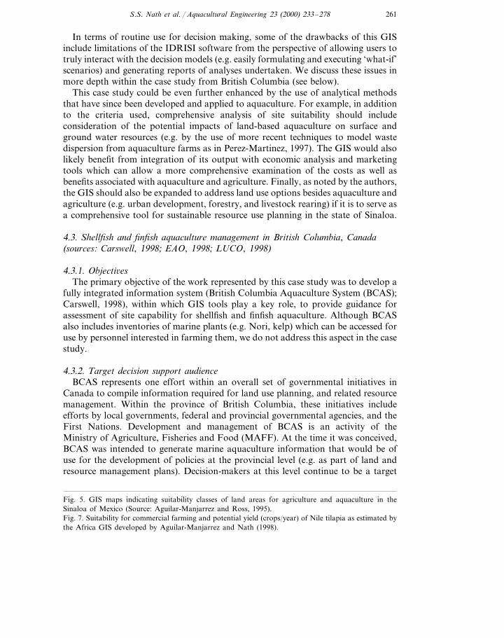
261S.S. Nath et al. / Aquacultural Engineering 23 (2000) 233–278
In terms of routine use for decision making, some of the drawbacks of this GISinclude limitations of the IDRISI software from the perspective of allowing users totruly interact with the decision models (e.g. easily formulating and executing ‘what-if’scenarios) and generating reports of analyses undertaken. We discuss these issues inmore depth within the case study from British Columbia (see below).
This case study could be even further enhanced by the use of analytical methodsthat have since been developed and applied to aquaculture. For example, in additionto the criteria used, comprehensive analysis of site suitability should includeconsideration of the potential impacts of land-based aquaculture on surface andground water resources (e.g. by the use of more recent techniques to model wastedispersion from aquaculture farms as in Perez-Martinez, 1997). The GIS would alsolikely benefit from integration of its output with economic analysis and marketingtools which can allow a more comprehensive examination of the costs as well asbenefits associated with aquaculture and agriculture. Finally, as noted by the authors,the GIS should also be expanded to address land use options besides aquaculture andagriculture (e.g. urban development, forestry, and livestock rearing) if it is to serve asa comprehensive tool for sustainable resource use planning in the state of Sinaloa.
4.3. Shellfish and finfish aquaculture management in British Columbia, Canada(sources: Carswell, 1998; EAO, 1998; LUCO, 1998)
4.3.1. Objecti6esThe primary objective of the work represented by this case study was to develop a
fully integrated information system (British Columbia Aquaculture System (BCAS);Carswell, 1998), within which GIS tools play a key role, to provide guidance forassessment of site capability for shellfish and finfish aquaculture. Although BCASalso includes inventories of marine plants (e.g. Nori, kelp) which can be accessed foruse by personnel interested in farming them, we do not address this aspect in the casestudy.
4.3.2. Target decision support audienceBCAS represents one effort within an overall set of governmental initiatives in
Canada to compile information required for land use planning, and related resourcemanagement. Within the province of British Columbia, these initiatives includeefforts by local governments, federal and provincial governmental agencies, and theFirst Nations. Development and management of BCAS is an activity of theMinistry of Agriculture, Fisheries and Food (MAFF). At the time it was conceived,BCAS was intended to generate marine aquaculture information that would be ofuse for the development of policies at the provincial level (e.g. as part of land andresource management plans). Decision-makers at this level continue to be a target
Fig. 5. GIS maps indicating suitability classes of land areas for agriculture and aquaculture in theSinaloa of Mexico (Source: Aguilar-Manjarrez and Ross, 1995).Fig. 7. Suitability for commercial farming and potential yield (crops/year) of Nile tilapia as estimated bythe Africa GIS developed by Aguilar-Manjarrez and Nath (1998).
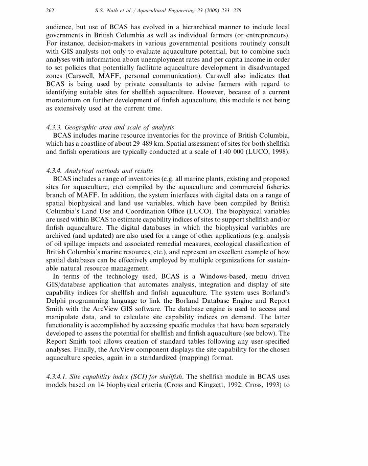
262 S.S. Nath et al. / Aquacultural Engineering 23 (2000) 233–278
audience, but use of BCAS has evolved in a hierarchical manner to include localgovernments in British Columbia as well as individual farmers (or entrepreneurs).For instance, decision-makers in various governmental positions routinely consultwith GIS analysts not only to evaluate aquaculture potential, but to combine suchanalyses with information about unemployment rates and per capita income in orderto set policies that potentially facilitate aquaculture development in disadvantagedzones (Carswell, MAFF, personal communication). Carswell also indicates thatBCAS is being used by private consultants to advise farmers with regard toidentifying suitable sites for shellfish aquaculture. However, because of a currentmoratorium on further development of finfish aquaculture, this module is not beingas extensively used at the current time.
4.3.3. Geographic area and scale of analysisBCAS includes marine resource inventories for the province of British Columbia,
which has a coastline of about 29 489 km. Spatial assessment of sites for both shellfishand finfish operations are typically conducted at a scale of 1:40 000 (LUCO, 1998).
4.3.4. Analytical methods and resultsBCAS includes a range of inventories (e.g. all marine plants, existing and proposed
sites for aquaculture, etc) compiled by the aquaculture and commercial fisheriesbranch of MAFF. In addition, the system interfaces with digital data on a range ofspatial biophysical and land use variables, which have been compiled by BritishColumbia’s Land Use and Coordination Office (LUCO). The biophysical variablesare used within BCAS to estimate capability indices of sites to support shellfish and/orfinfish aquaculture. The digital databases in which the biophysical variables arearchived (and updated) are also used for a range of other applications (e.g. analysisof oil spillage impacts and associated remedial measures, ecological classification ofBritish Columbia’s marine resources, etc.), and represent an excellent example of howspatial databases can be effectively employed by multiple organizations for sustain-able natural resource management.
In terms of the technology used, BCAS is a Windows-based, menu drivenGIS/database application that automates analysis, integration and display of sitecapability indices for shellfish and finfish aquaculture. The system uses Borland’sDelphi programming language to link the Borland Database Engine and ReportSmith with the ArcView GIS software. The database engine is used to access andmanipulate data, and to calculate site capability indices on demand. The latterfunctionality is accomplished by accessing specific modules that have been separatelydeveloped to assess the potential for shellfish and finfish aquaculture (see below). TheReport Smith tool allows creation of standard tables following any user-specifiedanalyses. Finally, the ArcView component displays the site capability for the chosenaquaculture species, again in a standardized (mapping) format.
4.3.4.1. Site capability index (SCI) for shellfish. The shellfish module in BCAS usesmodels based on 14 biophysical criteria (Cross and Kingzett, 1992; Cross, 1993) to
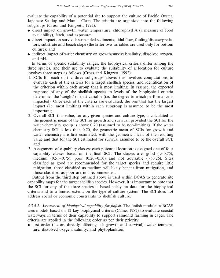
263S.S. Nath et al. / Aquacultural Engineering 23 (2000) 233–278
evaluate the capability of a potential site to support the culture of Pacific Oyster,Japanese Scallop and Manila Clam. The criteria are organized into the followingsubgroups (Cross and Kingzett, 1992):� direct impact on growth: water temperature, chlorophyll A (a measure of food
availability), fetch, and exposure;� direct impact on survival: suspended sediments, tidal flow, fouling/disease/preda-
tors, substrate and beach slope (the latter two variables are used only for bottomculture); and
� indirect impact of water chemistry on growth/survival: salinity, dissolved oxygen,and pH.In terms of specific suitability ranges, the biophysical criteria differ among the
three species, and their use to evaluate the suitability of a location for cultureinvolves three steps as follows (Cross and Kingzett, 1992):1. SCIs for each of the three subgroups above: this involves computations to
evaluate each of the criteria for a target shellfish species, and identification ofthe criterion within each group that is most limiting. In essence, the expectedresponse of any of the shellfish species to levels of the biophysical criteriadetermines the ‘weight’ of that variable (i.e. the degree to which performance isimpacted). Once each of the criteria are evaluated, the one that has the largestimpact (i.e. most limiting) within each subgroup is assumed to be the mostimportant;
2. Overall SCI: this value, for any given species and culture type, is calculated asthe geometric mean of the SCI for growth and survival, provided the SCI for thewater chemistry group is above 0.70 (assumed to be non-limiting). If the waterchemistry SCI is less than 0.70, the geometric mean of SCIs for growth andwater chemistry are first estimated, with the geometric mean of the resultingvalue and that for the SCI estimated for survival assumed to be the overall SCI;and
3. Assignment of capability classes: each potential location is assigned one of fourcapability classes based on the final SCI. The classes are: good (\0.75),medium (0.51–0.75), poor (0.26–0.50) and not advisable (B0.26). Sitesclassified as good are recommended for the target species and require littlemitigation, those classified as medium will likely benefit from mitigation, andthose classified as poor are not recommended.
Output from the third step outlined above is used within BCAS to generate sitecapability maps for the target shellfish species. However, it is important to note thatthe SCI for any of the three species is based solely on data for the biophysicalcriteria and to a limited extent, on the type of culture system. The SCI does notaddress social or economic constraints to shellfish culture.
4.3.4.2. Assessment of biophysical capability for finfish. The finfish module in BCASuses models based on 12 key biophysical criteria (Caine, 1987) to evaluate coastalwaterways in terms of their capability to support salmonid farming in cages. Thecriteria are applied in the following order as per their priority:� first order (factors directly affecting fish growth and survival): water tempera-
ture, dissolved oxygen, salinity, and phytoplankton;
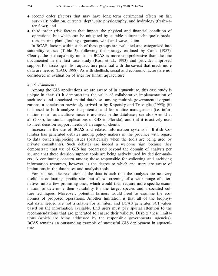
264 S.S. Nath et al. / Aquacultural Engineering 23 (2000) 233–278
� second order (factors that may have long term detrimental effects on fishsurvival): pollution, currents, depth, site physiography, and hydrology (freshwa-ter flow); and
� third order (risk factors that impact the physical and financial condition ofoperations, but which can be mitigated by suitable culture techniques): preda-tors, marine plants/fouling organisms, wind and wave action.In BCAS, factors within each of these groups are evaluated and categorized into
suitability classes (Table 3), following the strategy outlined by Caine (1987).Clearly, the site capability model in BCAS is more comprehensive than the onedocumented in the first case study (Ross et al., 1993) and provides improvedsupport for assessing finfish aquaculture potential with the caveat that much moredata are needed (EAO, 1998). As with shellfish, social and economic factors are notconsidered in evaluation of sites for finfish aquaculture.
4.3.5. CommentsAmong the GIS applications we are aware of in aquaculture, this case study is
unique in that: (i) it demonstrates the value of collaborative implementation ofsuch tools and associated spatial databases among multiple governmental organi-zations, a conclusion previously arrived to by Kapetsky and Travaglia (1995); (ii)it is used to both analyze site potential and for routine management (i.e. infor-mation on all aquaculture leases is archived in the databases; see also Arnold etal. (2000), for similar applications of GIS in Florida); and (iii) it is actively usedto meet decision support needs of a range of clients.
Increase in the use of BCAS and related information systems in British Co-lumbia has generated debates among policy makers in the province with regardto data ownership/pricing issues (particularly when the tools are being used byprivate consultants). Such debates are indeed a welcome sign because theydemonstrate that use of GIS has progressed beyond the domain of analysts perse, and that these decision support tools are being actively used by decision-mak-ers. A continuing concern among those responsible for collecting and archivinginformation resources, however, is the degree to which end users are aware oflimitations in the databases and analysis tools.
For instance, the resolution of the data is such that the analyses are not veryuseful in evaluating specific sites but allow screening of a wide range of alter-natives into a few promising ones, which would then require more specific exam-ination to determine their suitability for the target species and associated cul-ture techniques. Moreover, potential farmers would need to examine the eco-nomics of proposed operations. Another limitation is that all of the biophys-ical data needed are not available for all sites, and BCAS generates SCI valuesbased on the information available. End users must pay special attention to therecommendations that are generated to ensure their validity. Despite these limita-tions (which are being addressed by the responsible governmental agencies),BCAS remains an outstanding example of successful GIS deployment in aquacul-ture.
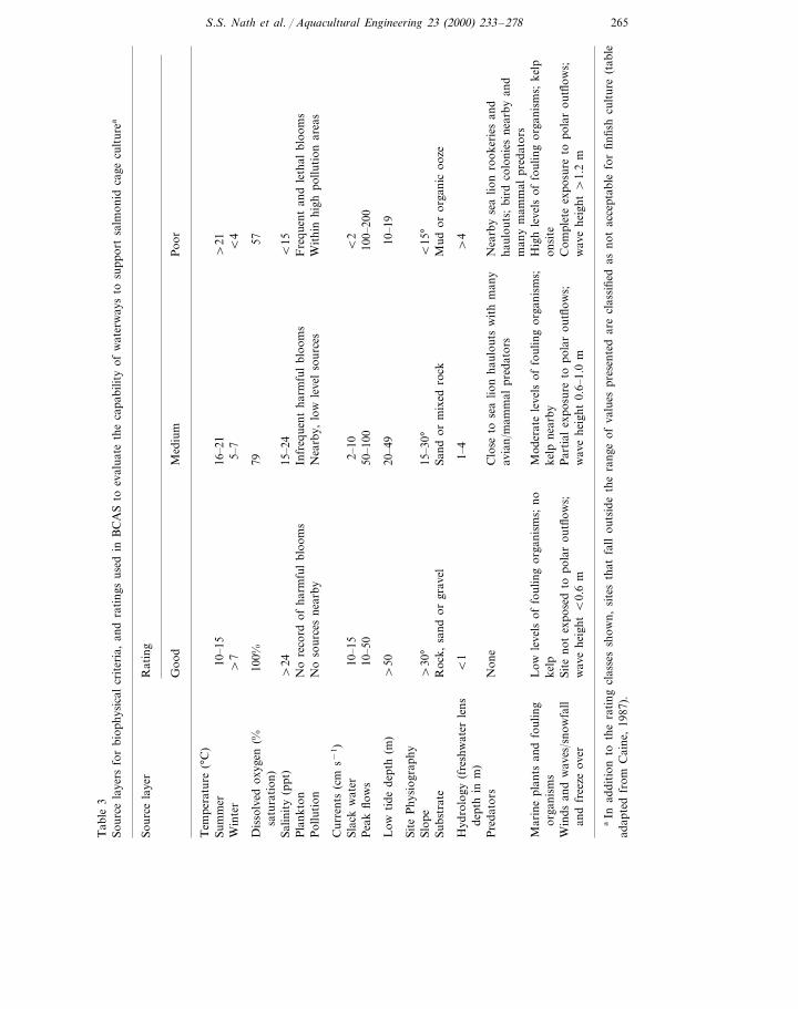
265S.S. Nath et al. / Aquacultural Engineering 23 (2000) 233–278
Tab
le3
Sour
cela
yers
for
biop
hysi
cal
crit
eria
,an
dra
ting
sus
edin
BC
AS
toev
alua
teth
eca
pabi
lity
ofw
ater
way
sto
supp
ort
salm
onid
cage
cult
urea
Rat
ing
Sour
cela
yer
Med
ium
Goo
dP
oor
Tem
pera
ture
(°C
)10
–15
16–2
1\
21Su
mm
erW
inte
r5–
7\
7B
4
100%
5779
Dis
solv
edox
ygen
(%sa
tura
tion
)\
2415
–24
B15
Salin
ity
(ppt
)N
ore
cord
ofha
rmfu
lbl
oom
sP
lank
ton
Infr
eque
ntha
rmfu
lbl
oom
sF
requ
ent
and
leth
albl
oom
sP
ollu
tion
Nea
rby,
low
leve
lso
urce
sN
oso
urce
sne
arby
Wit
hin
high
pollu
tion
area
s
Cur
rent
s(c
ms−
1)
10–1
52–
10B
2Sl
ack
wat
er10
0–20
010
–50
Pea
kflo
ws
50–1
00
\50
20–4
910
–19
Low
tide
dept
h(m
)
Site
Phy
siog
raph
yB
15°
15–3
0°Sl
ope
\30
°Su
bstr
ate
Sand
orm
ixed
rock
Roc
k,sa
ndor
grav
elM
udor
orga
nic
ooze
1–4
\4
B1
Hyd
rolo
gy(f
resh
wat
erle
nsde
pth
inm
)C
lose
tose
alio
nha
ulou
tsw
ith
man
yN
one
Pre
dato
rsN
earb
yse
alio
nro
oker
ies
and
haul
outs
;bi
rdco
loni
esne
arby
and
avia
n/m
amm
alpr
edat
ors
man
ym
amm
alpr
edat
ors
Hig
hle
vels
offo
ulin
gor
gani
sms;
kelp
Low
leve
lsof
foul
ing
orga
nism
s;no
Mar
ine
plan
tsan
dfo
ulin
gM
oder
ate
leve
lsof
foul
ing
orga
nism
s;ke
lpne
arby
onsi
teor
gani
sms
kelp
Win
dsan
dw
aves
/sno
wfa
llC
ompl
ete
expo
sure
topo
lar
outfl
ows;
Par
tial
expo
sure
topo
lar
outfl
ows;
Site
not
expo
sed
topo
lar
outfl
ows;
wav
ehe
ight\
1.2
mw
ave
heig
ht0.
6–1.
0m
wav
ehe
ightB
0.6
man
dfr
eeze
over
aIn
addi
tion
toth
era
ting
clas
ses
show
n,si
tes
that
fall
outs
ide
the
rang
eof
valu
espr
esen
ted
are
clas
sifie
das
not
acce
ptab
lefo
rfin
fish
cult
ure
(tab
lead
apte
dfr
omC
aine
,19
87).
266 S.S. Nath et al. / Aquacultural Engineering 23 (2000) 233–278
4.4. Inland aquaculture potential in Africa (source: Aguilar-Manjarrez and Nath,1998)
4.4.1. Objecti6esThe motivation for the current study was the pressing need for up-to-date
information that can be used to guide aquaculture development in Africa (WorldBank, 1996). Recently compiled, more comprehensive spatial databases for theAfrican continent as well as advances in spatial methods to assess fish farmingpotential provided an additional incentive to conduct the study.
4.4.2. Target decision support audienceThe primary audience for continental-scale and country-level estimates of inland
aquaculture potential across Africa potentially include national/international tech-nical assistance agencies, large aquaculture corporations, and the internationaldonor community. At this time, however, we are unaware of any instances wherethe outcomes from the study have actually been used for project assessment or tomeet other decision support needs.
4.4.3. Geographic area and scale of analysisGIS analyses were conducted for the entire African continent, with the exception
of Madagascar for which some essential weather datasets were not available. Thestudy examines the extent to which ‘sites’ (essentially areas 5 km×5 km in sizecorresponding to 3¦ grid cells) satisfy criteria for small-scale and commercial fishfarming, and assesses the performance of three index fish species (Nile tilapia,African catfish, and Common carp) under such farming systems.
4.4.4. Analytical methods and resultsThe basis of the present study is conceptually similar to traditional studies for
assessing aquaculture potential (Muir and Kapetsky, 1988; Born et al., 1994).However, use of a GIS greatly enhanced the evaluation, especially with regard tothe application of objective decision-making methods, quantifying limitations im-posed by different production factors, providing estimates of the predicted fishfarming potential, and visualizing outcomes. GIS analyses were primarily accom-plished using the ArcInfo system, although other software tools (IDRISI, ERDASand IDA) were also used.
Spatial analysis was limited to assessment of land-based inland aquaculturepotential, which for practical purposes implies pond systems. The potential foraquaculture in large inland water bodies (e.g. using cage culture) and in oceanwaters was not assessed. This case study provides a good example of dataconsolidation from multiple sources (Table 4). Analytical procedures in the studywere largely derived from previous efforts (Aguilar-Manjarrez, 1996; Kapetsky andNath, 1997), and involved three phases:1. criteria identification, classification, and standardization;2. integration of primary criteria; and
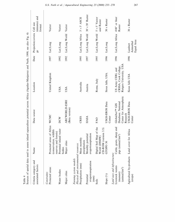
267S.S. Nath et al. / Aquacultural Engineering 23 (2000) 233–278
Tab
le4
Sour
ces
ofsp
atia
lda
taus
edto
asse
ssin
land
aqua
cult
ure
pote
ntia
lac
ross
Afr
ica
(Agu
ilar-
Man
jarr
ezan
dN
ath,
1998
;se
eal
soF
ig.
4)
Cel
lsi
zeN
ame
Cri
teri
aca
tego
ryan
dD
ata
sour
ceL
ocat
ion
Dat
eP
roje
ctio
n/co
vera
asso
ciat
edfa
ctor
s(m
inut
es)
and
gefo
rmat
Con
stra
ints
Pro
tect
edar
eas
ofA
fric
aL
at/L
ong
Pro
tect
edar
eas
WC
MC
Vec
tor
Uni
ted
Kin
gdom
1997
(con
serv
atio
n,w
ildlif
ere
serv
esan
dfo
rest
s)P
eren
nial
inla
ndw
ater
Vec
tor
DC
WW
ater
bodi
esU
SA19
92L
at/L
ong
bodi
esM
ajor
citi
esA
RC
WO
RL
D-E
SRI
Vec
tor
USA
Maj
orci
ties
1992
Lat
/Lon
gW
orld
(Bet
ave
rsio
n)
Far
min
gsy
stem
mod
els
Phy
sica
lan
den6i
ronm
enta
lre
sour
ces
Pre
cipi
tati
on(m
m)
Mea
nm
onth
ly3%
×3%
ASC
IIC
RE
SA
ustr
alia
1995
Lat
/Lon
gA
fric
apr
ecip
itat
ion
30%×
30%
Ras
ter
Pot
enti
alM
onth
lypo
tent
ial
IIA
SAA
ustr
ia19
97L
at/L
ong
Wor
ldev
apot
rans
pira
tion
evap
otra
nspi
rati
on(m
m)
Dig
ital
Soil
Map
ofth
eL
at/L
ong
Wor
ld5%
×5%
Vec
tor
Soils
FA
OR
ome,
Ital
y19
95W
orld
(DSM
W)
and
Ras
ter
CD
-RO
M(v
ersi
on3.
5)G
TO
PO
30U
SGS-
ER
OS
Dat
aSi
oux
falls
,U
SA.
1996
Lat
/Lon
g30
sR
aste
rSl
ope
(%)
Cen
ter
Lan
dus
esan
din
fras
truc
ture
US
Arm
yC
ER
Lan
dC
attl
e,go
ats,
shee
pan
d4%
48¦
orfin
erG
loba
lArc
™G
IS19
96L
ives
tock
was
tes
Lat
/Lon
gA
fric
aC
RSS
A,
Coo
kC
olle
ge,
pigs
(ani
mal
/km
2)
Dat
abas
e.N
atio
nal
Ras
ter
(man
ure)
(ani
mal
/km
2)
Cen
ter
for
Atm
osph
eric
Rut
gers
Uni
vers
ity.
USA
Res
earc
hA
gric
ultu
ral
by-p
rodu
cts
Lan
dco
ver
for
Afr
ica
30s
Ras
ter
USG
S-E
RO
SD
ata
Siou
xfa
llsU
SA19
96L
ambe
rt(c
rops
)A
zim
utha
lC
ente
rE
qual
Are
a
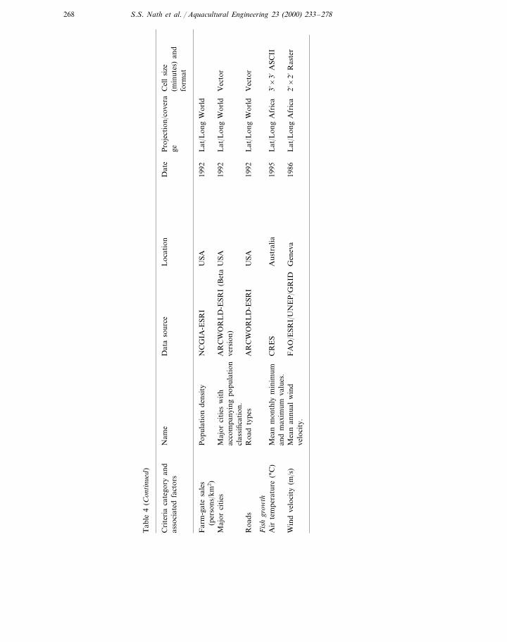
268 S.S. Nath et al. / Aquacultural Engineering 23 (2000) 233–278
Tab
le4
(Con
tinu
ed)
Pro
ject
ion/
cove
raN
ame
Cri
teri
aca
tego
ryan
dC
ell
size
Dat
aso
urce
Loc
atio
nD
ate
asso
ciat
edfa
ctor
sge
(min
utes
)an
dfo
rmat
Lat
/Lon
gW
orld
Far
m-g
ate
sale
sP
opul
atio
nde
nsit
yN
CG
IA-E
SRI
USA
1992
(per
sons
/km
2)
USA
1992
Lat
/Lon
gW
orld
Vec
tor
Maj
orci
ties
AR
CW
OR
LD
-ESR
I(B
eta
Maj
orci
ties
wit
hac
com
pany
ing
popu
lati
onve
rsio
n)cl
assi
ficat
ion.
Vec
tor
AR
CW
OR
LD
-ESR
IU
SAR
oads
Roa
dty
pes
1992
Lat
/Lon
gW
orld
Fis
hgr
owth
1995
Mea
nm
onth
lym
inim
umL
at/L
ong
Afr
ica
3%×
3%A
SCII
CR
ES
Aus
tral
iaA
irte
mpe
ratu
re(°
C)
and
max
imum
valu
es.
Lat
/Lon
gA
fric
a2%
×2%
Ras
ter
Gen
eva
Win
dve
loci
ty(m
/s)
Mea
nan
nual
win
d19
86F
AO
/ESR
I/U
NE
P/G
RID
velo
city
.
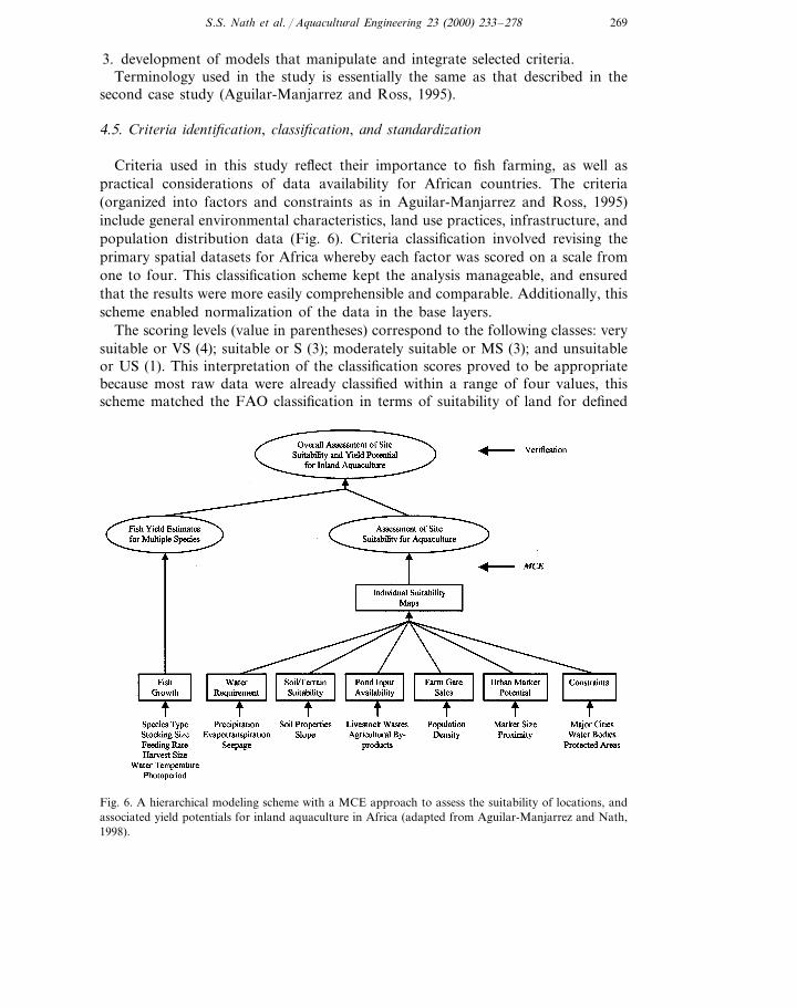
269S.S. Nath et al. / Aquacultural Engineering 23 (2000) 233–278
3. development of models that manipulate and integrate selected criteria.Terminology used in the study is essentially the same as that described in the
second case study (Aguilar-Manjarrez and Ross, 1995).
4.5. Criteria identification, classification, and standardization
Criteria used in this study reflect their importance to fish farming, as well aspractical considerations of data availability for African countries. The criteria(organized into factors and constraints as in Aguilar-Manjarrez and Ross, 1995)include general environmental characteristics, land use practices, infrastructure, andpopulation distribution data (Fig. 6). Criteria classification involved revising theprimary spatial datasets for Africa whereby each factor was scored on a scale fromone to four. This classification scheme kept the analysis manageable, and ensuredthat the results were more easily comprehensible and comparable. Additionally, thisscheme enabled normalization of the data in the base layers.
The scoring levels (value in parentheses) correspond to the following classes: verysuitable or VS (4); suitable or S (3); moderately suitable or MS (3); and unsuitableor US (1). This interpretation of the classification scores proved to be appropriatebecause most raw data were already classified within a range of four values, thisscheme matched the FAO classification in terms of suitability of land for defined
Fig. 6. A hierarchical modeling scheme with a MCE approach to assess the suitability of locations, andassociated yield potentials for inland aquaculture in Africa (adapted from Aguilar-Manjarrez and Nath,1998).
270 S.S. Nath et al. / Aquacultural Engineering 23 (2000) 233–278
uses, and the same methodology had been successfully used in aquaculture (Kapet-sky, 1994; Aguilar-Manjarrez, 1996; Kapetsky and Nath, 1997). The interpretationof suitability classes is as follows (Kapetsky and Nath, 1997): ‘The VS levelprovides a situation in which minimum time or investment is required in order todevelop fish farming. For a level classified as S, modest time and investment arerequired, while if MS, significant interventions may be required before fish farmingoperations can be conducted. If the suitability level is US, the time or cost, or both,are too great to be worthwhile for fish farming.’
In accordance with the suitability classification scheme, ranges of data (orthresholds) that pertain to a desired level of suitability for each of the criteria hadto be chosen. Selection of such thresholds involved interpretation of the dataselected, a process that was guided with literature research (e.g. for soil types) andopinions from expert staff at FAO.
4.6. Integration of primary criteria
In this phase, selected and scored criteria were grouped into a series of sub-mod-els (Kapetsky, 1994; Aguilar-Manjarrez, 1996; Kapetsky and Nath, 1997). Sub-models for commercial fish farming assessment included water requirement,soils/terrain suitability, pond input availability, farm-gate sales, and urban marketpotential (Fig. 6). All of these sub-models (with the exception of urban marketpotential) were used to assess small-scale farming opportunities. The rationale foruse of these sub-models was based on previous work (Kapetsky and Nath, 1997).
As opposed to Aguilar-Manjarrez and Ross (1995) who integrated constraintsonly after individual suitability maps were generated (Fig. 4), Aguilar-Manjarrezand Nath (1998) included constraints within each sub-model outcomes (Fig. 6).This was because when suitability classes were developed, it was found that some ofthem were located within constraint regions and thus affected the suitability ranges.In the Sinaloa case study, however, this was not the situation and it was convenientto deal with constraints following application of the MCE technique.
4.7. De6elopment of the models
The third major analytical procedure involved the development and evaluation ofmodels to estimate the potential for small-scale and commercial fish farming inponds. Two groups of models were used: farming systems models to assess landsuitability for aquaculture (involving use of MCE to integrate sub-models devel-oped in the previous phase), and simulation models to estimate fish yield potential(in crops/year).
Use of the MCE approach involved consultations among one of the authors (J.Aguilar-Manjarrez) and four aquaculture experts with the objective of arriving atweights for the farming systems sub-models as a measure of their importanceto small-scale and commercial farming systems. For small-scale farming, finalweights used for the water requirement, pond input availability, soils/terrainsuitability, and farm-gate sales sub-models were 0.56, 0.26, 0.12 and 0.06, respec-
271S.S. Nath et al. / Aquacultural Engineering 23 (2000) 233–278
tively. Corresponding weights for commercial farming were 0.30, 0.04, 0.13, and0.07, respectively, with the urban market potential sub-model receiving a weightof 0.46. Thus, water requirement and pond input availability were identified asbeing most important for small-scale farming, whereas urban market potentialand water requirement were most important for commercial fish farming. Weightsassigned to all of the sub-models for each fish farming category were applied togenerate integrated suitability maps.
Two linked simulation models were also used in this study. The first of this wasused to generate mean monthly water temperature profiles across the Africancontinent. This output was then used, among other input parameters, in a bioen-ergetics model (Nath, 1996) to estimate fish yield potential (in crops/year) for theNile tilapia, African catfish, and Common carp under small-scale and commercialfarming conditions. The resulting output was exported to GIS for further analysisand manipulation. For simplicity, all annual production results were reported bydividing the ranges estimated under small-scale and commercial farming scenariosinto four quarters (Q).
Suitability maps from the farming system models were overlaid with those fromthe bioenergetics model to reach a combined evaluation that indicated the coin-cidence of each land quality suitability class with a range of yield potential.Finally, existing fish farm locations (obtained by the use of GPS with additionalfield work to determine on-site production conditions) from four countries(Kenya, Malawi, Uganda and Zimbabwe) were used to verify the accuracy of theresults.
4.8. Results
A very small subset of the results discussed by Aguilar-Manjarrez and Nath(1998) are presented here due to space restrictions. From the perspective of acontinental overview, despite multiple constraints imposed by the need to meetland quality requirements for both fish farming systems and favorable fish yields,over 15% of Africa has land areas scored as VS-1stQ for the three fish species andfor both types of culture systems (Table 5). The largest surface area scored in theVS-1stQ combinations was found for common carp in the small-scale model.Suitability ranges for Nile tilapia were markedly more restrictive than the othertwo species in the VS-1stQ, in large part because of its more restricted range ofrequired water temperatures.
The major difference between the two culture systems was that the commercialfarming results showed patchy distributions due to the urban market potentialsub-model (Fig. 7), a feature that was not present in the small-scale model results.Very suitable sites with 1stQ yield ranges for both commercial and small-scalefarming of the three fish species are located across Africa between 14°–20° S and17°–40° E. Again, however, the importance of the urban market potential sub-model in the commercial farming scenario does identify areas not identified in thesmall-scale model as having higher or lower potential such as the DemocraticRepublic of the Congo and South Africa, respectively.
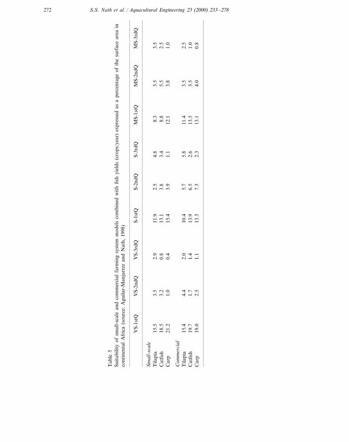
272 S.S. Nath et al. / Aquacultural Engineering 23 (2000) 233–278
Tab
le5
Suit
abili
tyof
smal
l-sc
ale
and
com
mer
cial
farm
ing
syst
emm
odel
sco
mbi
ned
wit
hfis
hyi
elds
(cro
ps/y
ear)
expr
esse
das
ape
rcen
tage
ofth
esu
rfac
ear
eain
cont
inen
tal
Afr
ica
(sou
rce:
Agu
ilar-
Man
jarr
ezan
dN
ath,
1998
)
S-1s
tQS-
2ndQ
S-3r
dQM
S-1s
tQM
S-2n
dQM
S-3r
dQV
S-2n
dQV
S-3r
dQV
S-1s
tQ
Sm
all-
scal
e11
.92.
54.
88.
33.
53.
5T
ilapi
a15
.53.
52.
93.
48.
85.
52.
53.
8C
atfis
h13
.10.
83.
218
.515
.43.
91.
112
.13.
81.
01.
0C
arp
0.4
21.2
Com
mer
cial
5.8
11.4
3.5
4.4
2.5
15.4
2.0
10.4
5.7
Tila
pia
2.6
13.5
3.5
1.0
Cat
fish
19.7
1.7
1.4
13.9
6.5
2.3
13.1
4.0
0.8
7.3
2.5
Car
p19
.013
.31.
1
273S.S. Nath et al. / Aquacultural Engineering 23 (2000) 233–278
From the perspective of a country-level overview, potential areas for small-scalefarming of Nile tilapia are also smaller when compared to the other two species. Only11 African countries were scored as VS-1stQ in 50% or more of their surface area;however, the ranks of these countries are quite similar when compared to the othertwo fish species. For African catfish, 14 countries have 50% or more of their landarea scored as VS-1stQ; an additional seven countries possess this score in more than25% of their area. These results are similar to those for Common carp; however, afew more countries which offer VS-1stQ and S-1stQ possibilities are favored for thisspecies.
At the country-level, commercial farming results are similar to those for small-scalefarming, except that the spatial distribution of the potential sites for commercialfarming is greater for the VS-1stQ, VS-2ndQ and S-2ndQ ranges resulting in a largernumber of countries where these combinations coincide for all three fish species. Inall, 11 countries that meet or exceed S-1stQ requirements for 25% or more of theirnational areas for African catfish, nine for common carp and eight for Nile tilapia.Liberia, Sierra Leone, Ivory Coast, and Equatorial Guinea were found to be the mostfavorable countries for the three fish species and for both culture systems.
In summary, results from this work confirm Kapetsky’s (Kapetsky, 1994) findingsthat the potential for inland aquaculture in Africa is high. The final fish farmingpotential estimates for the three species together show that about 37 and 43% of theAfrican surface contains areas with at least some potential for small-scale andcommercial farming, respectively. The most significant finding of the study was that15% of the same areas have the highest suitability score. This implies that forsmall-scale fish farming, from 1.3 to 1.7 crops/year of Nile tilapia, 1.9–2.4 crops/yearof African catfish and 1.6–2.2 crops/year of Common carp can be achieved in theseareas. Similar ranges for commercial farming are: 1.6–2.0 crops/year of Nile tilapia,1.3–1.7 crops/year of African catfish and 1.2–1.5 crops/year of Common carp. Ingeneral, the verification exercises conducted for four African countries indicated thatoutcomes generated by the GIS were consistent with on-the-ground evaluations offish farming suitability.
4.8.1. CommentsEstimates of area with potential (or lack of it) for fish farming development in this
study were influenced by many factors, some of which originated from datainaccuracy, their spatial and temporal availability, the analytical approach and theunderlying assumptions adopted. However, the increasing availability of data andgreater capabilities of computer technology suggest an expanded role of GIS forlarge-scale assessments of aquaculture potential, and many of the problems affectingresults of this study will likely be minimized or eliminated as more data becomesavailable, and more experience is gained with aquaculture-oriented GIS.
One of the limitations of this study was the use of a single set of models (e.g.threshold selection and grouping of various criteria into commercial and small-scalemodels) to evaluate inland aquaculture potential. This limitation was necessarybecause of the lack of adequate information comparable across all countries thatcould be selectively used in the analyses, and because of the strategic nature (i.e.
274 S.S. Nath et al. / Aquacultural Engineering 23 (2000) 233–278
continental-scale focus) of the study. For example, the use of a global threshold of300 individuals/km2 for population density at which land was assumed to becometoo expensive for small-scale fish farming may not apply to all situations as indicatedby the verification exercise conducted for Kenya. Nevertheless, it should be possibleto use the GIS together with additional country-specific information, to generateassessments that are more suitable for national-level planning activities.
The verification exercise provided an important insight into the value of suchstrategic studies of fish farming opportunities ‘prior’ to encouraging its development.For instance, Zimudzi (1997) reported that after an initial enthusiasm for aquacul-ture in the 1980s, the majority of Zimbabwean farmers have stopped fish farmingdue to a variety of reasons including water shortage, poor yields of Nile tilapia dueto low water temperatures, and unpredictable survival rates. These same areas wereclassified as being only marginally suitable in the GIS.
As previously noted, despite the apparent value of the GIS outcomes for policyplanning efforts in Africa, it is not clear if the results are being used by decision-makers. This may be due to a number of factors including: (i) a lack of awarenessamong such key personnel that GIS work to assess aquaculture potential has beenconducted; (ii) a lack of appreciation of the methods used and outcomes generated;(iii) low priority of aquaculture development efforts among international donors;and (iv) constraints imposed by the poor state of most African governmentalagencies involved in aquaculture development. These issues must be investigatedfurther if progress is to be made with regard to actual use of GIS output fordevelopment and planning efforts.
5. Future trends in GIS
Geographic information systems science and technology, like many other areas ofcomputing and information management, continues to evolve at a rapid pace.Advances are being made with regard to ease of use, manipulation of large (\100MB) datasets, interoperability of databases among different systems, and in thecollection and preprocessing of datasets. Perhaps the most significant developmentis an increasing trend towards the use of GIS as a component of a larger decisionsupport system. This has been facilitated by the development of industry-widecomponent standards and object-oriented program designs. For example, thecurrent release of ArcInfo (Version 8; ESRI, Inc.) has replaced the monolithicapplication model with an object-based component model that facilitates embeddingGIS technology in broader application frameworks. Thus, application developerscan deploy GIS-enabled applications by incorporating software components sup-porting geographic manipulation and visualization functions that are needed fortheir specific application, in conjunction with any other component-based function-ality (e.g. reporting modules, database support, etc.) required for the application.This allows developers to produce customized applications utilizing spatial datasets,and has particular usefulness in allowing more robust interaction between modelsand GIS datasets, and in connecting relational database systems to map displays.
275S.S. Nath et al. / Aquacultural Engineering 23 (2000) 233–278
Further, the need to purchase a single, large software application (most functional-ity of which is rarely used) is somewhat obviated.
Another area in which GIS is playing an increasingly important role is inlandscape visualization and ‘futuring’. Combined systems which model change in awatershed or landscape resulting from different land management strategies, andallow visualization of those changes in three dimensions, are becoming valuabletools for resource managers and stakeholders to better understand the implicationsof these strategies. This often takes the form of ‘virtual photographs’ where GISdatasets are mapped onto elevation grids, with appropriate visual ‘textures’ mappedinto each polygon displayed. Results of such operations can be very realistic photosimulations of what a particular landscape might actually look like under aparticular set of assumptions. In many respects, this trend mirrors the increasinguse of watersheds as the basic unit of analysis in natural resource managementdomains. Kapetsky (1998, 1999) is of the opinion that this trend will becomeincreasingly used in both inland fisheries assessments, and aquaculture as well.
Technological progress continues to be made in the acquisition of spatiallyexplicit datasets. Increasingly, remote sensed data are becoming available from arich set of satellite sources and from lower-altitude aerial fly-overs. A substantialcommercial industry focused on developing and supplying a broad range ofdatasets has recently arisen. As previously indicated, the internet has greatlyfacilitated the distribution of datasets of all types, and most government agenciesare beginning to distribute many datasets online. The cost of electronic storage(often less than $20/GB) and increasing capabilities of personal computers isallowing sophisticated GIS analyses to be readily accomplished by inexpensiveworkstations. Finally, a host of mobile data collection devices, ranging frompen-driven handheld computers to GPS units and laser range finders are facilitatingmore efficient spatial data collection; these will only increase in their sophisticationand ease of use.
Given information technology trends, there can be little doubt that future GIStools will provide a range of functions embedded in various components that can betailored for specific uses. However, barriers with regard to actually using these toolsfor real world decision making merit special attention (that has not been forthcom-ing) and will need to be overcome if GIS is to play an integral role in aquaculturedevelopment and management. More specifically, there is the continuing need forappreciation workshops targeted towards decision-makers (i.e. end users) anddomain experts to expand knowledge about GIS applications, and the need forrelevant coursework in aquaculture/fisheries curricula at the university level (Kapet-sky and Travaglia, 1995). Such training and education efforts can go a long waytowards making GIS a routine analytical tool in the aquaculture domain. Sympo-siums such as the First International Symposium on Fishery Sciences recently heldin the US (Seattle; March 2–4, 1999) are also valuable in this regard. Finally,organizations and individuals must facilitate the migration of GIS tools from therealm of the academic towards an environment within which analysts, subjectmatter experts and end users can fruitfully collaborate to address issues relevant tothe sustainable growth of aquaculture. Work conducted by various governmental
276 S.S. Nath et al. / Aquacultural Engineering 23 (2000) 233–278
agencies in the province of British Columbia (Canada) provides a useful model inthis regard, and demonstrates the value of inter- and intra-organizational collabora-tion with regard to strategic natural resource management initiatives, of whichaquaculture is only one component.
Acknowledgements
We acknowledge the assistance and information provided by Barron Carswell(MAFF, BC) and Mark Zacharias (LUCO, BC) with regard to the use of GIS foraquaculture management in British Columbia. Dr James M. Kapetsky (FAO), apioneer in the use of GIS for aquaculture and fisheries, has provided much adviceover the years and furnished information that was used in the preparation of thispaper. The senior author (S.S. Nath) acknowledges support provided by theDepartment of Biological and Agricultural Engineering at the University of Geor-gia, Athens, GA during the preparation of this manuscript.
References
Adams, J.L., 1986. Conceptual Blockbusting: A Guide to Better Ideas, 3rd ed. Addison-Wesley, Reading,MA, P. 161.
Aguilar-Manjarrez, J., 1992. Construction of a GIS for Tobasco State Mexico. Establishment of technicaland social decision models for aquaculture development. MSc Thesis, University of Stirling, UK.
Aguilar-Manjarrez, J., 1996. Development and evaluation of GIS-based models for planning andmanagement of coastal aquaculture: a case study in Sinaloa, Mexico. PhD Thesis. Institute ofAquaculture, University of Stirling, Scotland, UK.
Aguilar-Manjarrez, J., Nath, S.S., 1998. A strategic reassessment of fish farming potential in Africa.CIFA Technical paper. 32, FAO, Rome. http://www.fao.org/docrep/w8522e/w8522e00.htm.
Aguilar-Manjarrez, J., Ross, L.G., 1995. Geographical information systems (GIS), environmental modelsfor aquaculture development in Sinaloa state, Mexico. Aquaculture Int. 3, 103–115.
ALCOM, 1998. The SADC Water Resource Database. http://www.fao.org/WAICENT/FAOINFO/FISHERY/alcom/alcom.htm.
Ali, C.Q., Ross, L.G., Beveridge, M.C.M., 1991. Microcomputer spreadsheets for the implementation ofGeographical Information Systems in aquaculture. A case study on carp in Pakistan. Aquaculture 92,199–205.
Ambler, S.W., 1998. Building object applications that work. SIGS Books, Cambridge University Press,New York, 506 pp.
Arnold, W.S., Norris, H.A., White, M.W., 2000. Integrated resource management using geographicalinformation system technology: shellfish aquaculture in Florida, USA. Aquacultural Eng., in press.
Ben Mustafa, S., 1994. Identification et Preselection de Sites Potentiels pour l’Aquaculture sur le LittoralTunisien par Teledetection. Centre National de Teledetection, Tunis.
Born, A.F., Verdegem, M.C.J., Huisman, E.A., 1994. Macro-economic factors influencing worldaquaculture development. Aquaculture Fisheries Manage. 25, 519–536.
Burrough, P.A., 1986. Principles of Geographic Information Systems, 1st ed. Oxford University Press,New York 336 pp.
Burrough, P.A., McDonnell, 1998. Principles of Geographic Information Systems, 2nd ed. OxfordUniversity Press, New York.
Caine, G.C., 1987. Biophysical criteria for siting salmon farms in British Columbia. B.C. Min. Agric.Fish. Food, Aquaculture and Commercial Fisheries Branch.
277S.S. Nath et al. / Aquacultural Engineering 23 (2000) 233–278
Campbell, H., 1994. How effective are GIS in practice? A case study of British local government. Int.J. Geogr. Information Sys. 8, 309–325.
Campbell, H., Masser, I., 1995. GIS and Organizations: How Effective are GIS in Practice? Taylor andFrancis, London.
Carswell, B., 1998. BCAS: an information system for aquaculture and marine resource planning.Ministry of Agriculture, Fisheries and Food, British Columbia. Unpublished report.
Chimowa, M., Nugent, C., 1993. A fisheries GIS for Zimbabwe: an initial analysis of the numbers,distribution and size of Zimbabwe’s dams. AGRITEX Fisheries Unit-Technical Report.
Cross, S.F., 1993. Assessing shellfish culture capability in coastal British Columbia: sampling designconsiderations for extensive data acquisition surveys. Aquametrix Res. Prepared for B.C. Min. Agric.Fish. Food.
Cross, S.F., Kingzett, B.C., 1992. Biophysical criteria for shellfish culture in British Columbia: a sitecapability evaluation system. Aquametrix Res. Prepared for B.C. Min. Agric. Fish. Food.
EAO, 1998. The salmon aquaculture review final report, Environmental Assessment Office, Governmentof British Columbia, Canada. http://eaoluco-web.eao.gs.gov.bc.ca/project/AQUACULT/SALMON/report/toc.htm.
Eastman, J.R. 1993. IDRISI version 4.1. Update Manual. Clark Laboratories for CartographicTechnology and Geographic Analysis. Clark University, Worcester, MA, USA.
Faber, B.G., Wallace, W.W., Croteau, K., Thomas, V.L., Small, L.R., 1997. Active response GIS: anarchitecture for interactive resource modeling. Proceedings of the GIS ’97 Annual Symposium onGeographical Information Systems, Vancouver, BC.
Kapetsky, J.M., 1989. A geographical information system for aquaculture development in Johore State.FI: TCP/MAL/6754 Field Document. FAO, Rome.
Kapetsky, J.M., 1994. A strategic assessment of warm-water fish farming potential in Africa. CIFATechnical Paper, 27, FAO, Rome.
Kapetsky, J.M., 1998. Geography and constraints on inland fishery enhancements. In: Petr, T. (Ed.),Inland Fishery Enhancements. Papers presented at the FAO/DFID Expert Consultation on InlandFishery Enhancements. Dhaka, Bangladesh, 7–11 April 1997. FAO Fisheries Technical Paper. No.374. Rome, FAO. pp. 37–63.
Kapetsky, J.M., 1999. Strategic assessments of the potential for increasing fish production from inlandwaters. Paper presented at the First International Symposium on GIS in Fisheries Sciences, March2–4, 1999, Seattle, Washington, USA.
Kapetsky, J.M., Nath, S.S., 1997. A strategic assessment of the potential for freshwater fish farming inLatin America. COPESCAL Technical Paper N. 10. FAO, Rome.
Kapetsky, J.M., Travaglia, C., 1995. Geographical information systems and remote sensing: an overviewof their present and potential applications in aquaculture. In: Nambiar, K.P.P., Singh, T. (Eds.),AquaTech ’94: Aquaculture Towards the 21st Century. INFOFISH, Kuala Lumpur, pp. 187–208.
Kapetsky, J.M., McGregor, L., Nanne, H.E., 1987. A geographical information system and satelliteremote sensing to plan for aquaculture development: a FAO-UNEP/GRID cooperative study inCosta Rica. FAO Fish. Tech. Paper 287.
Kapetsky, J.M., Hill, J.M., Worthy, D.L., 1988. A geographical information system for catfish farmingdevelopment. Aquaculture 68, 311–320.
Kapetsky, J.M., Hill, J.M., Worthy, D.L., Evans, D.L., 1990a. Assessing potential for aquaculturedevelopment with a geographic information system. J. World Aqua. Soc. 21, 241–249.
Kapetsky, J.M., Wijkstrom, U.N., MacPherson, N.J., Vincke, M.M.J., Ataman, E., Caponera, F.,1990b. Where are the best opportunities for fish farming in Ghana? The Ghana aquaculturegeographical information system as a decision-making tool. FAO Field Technical Report 5, FI:TCP/GHA/0051, FAO, Rome.
Legault, J.A., 1992. Using a geographic information system to evaluate the effects of shellfish closurezones on shellfish leases, aquaculture and habitat availability. Can. Tech. Rep. Fish. Aquat. Sci.1882E: iv+10.
LUCO, 1998. Guide to spatial land and resource information in LRMP. Land Use and CoordinationOffice, British Columbia. http://www.luco.gov.bc.ca/lrmp/spatial/marine.htm.
Meaden, G.J., 1987. Where should trout farms be in Britain? Fish Farmer March/April, 33–35.
278 S.S. Nath et al. / Aquacultural Engineering 23 (2000) 233–278
Meaden, G.J., Kapetsky, J.M., 1991. Geographical Information Systems and Remote Sensing in InlandFisheries and Aquaculture. FAO Fisheries Technical Paper, No. 318.
Merkhofer, M.W., 1998. Assessment, refinement and narrowing of options. In: Dale, V.H., English,M.R. (Eds.), Tools to Aid Environmental Decision Making. Springer-Verlag, New York, pp.231–281.
Muir, J.F., Kapetsky, J.M., 1988. Site selection decisions and project cost: the case of brackish waterpond systems. Aquaculture engineering, Technologies for the Future, Institution of ChemicalEngineers Symposium Series No. 111. EFCE Publication Series, 66: 45–63.
Nath, S.S., 1996. Development of a decision support system for pond aquaculture. PhD Dissertation,Oregon State University, Corvallis, OR.
Osleeb, J.P., Kahn, S., 1998. Integration of geographic information. In: Dale, V.H., English, M.R.(Eds.), Tools to Aid Environmental Decision Making. Springer-Verlag, New York, pp. 161–189.
Paw, J.N., Domingo, F., Alojado, Z.N., Guiang, J., 1994. Land resource assessment for brackishwaterdevelopment in Lingayen Gulf area, Philippines. Technical Report on the Geographical InformationSystems Application for Coastal Area Management and Planning, Lingayen Gulf Area, Philippines,Part II.
Perez-Martinez, O., 1997. Modelling fish farm waste dispersal using GIS. M.Sc. Thesis. University ofStirling, Scotland.
Ross, L.G., 1998. The use of Geographical Information Systems in Aquaculture: A Review. Paperpresented at I Congreso Nacional de Limnologia, Michoacan, Mexico. November 1998.
Ross, L.G., Mendoza, E.A., Beveridge, M.C.M., 1993. The application of geographical informationsystems to site selection for coastal aquaculture: an example based on salmonid cage culture.Aquaculture 112, 165–178.
Saaty, T., 1980. The Analytic Hierarchy Process. McGraw-Hill, New York.Scott, P.C., Cansado, S., Ross, L.G., 1998. A GIS-assisted mollusc culture potential determination for
Sepetiba Bay, Brazil. Paper presented at the GIS Planet ’98 Conference, 7–11 September, 1998.Lisbon. Portugal.
Senge, P.M., 1990. The Fifth Discipline: The Art and Practice of the Learning Organization. BantamDoubleday, New York.
Thompson, S.A., 1998. Water Use, Management, and Planning in the United States. Academic Press,New York 371 pp.
Voland, C., 1992. Engineering by Design. Addison-Wesley Longman, Inc., Reading, MA, 547 pp.World Bank, 1996. Tropical aquaculture development: Research needs. World Bank Technical Paper
No. 151, Fisheries Series. The World Bank, Washington, DC.Zimudzi, F., 1997. Locations and Characteristics of Fish Farms in Zimbabwe for Verification Work of
a Strategic Re-assessment of Fish Farming Potential in Africa. FAO, Rome.
.