LIBRARY RESEARCH REPORTS DIVISION NAVAL POSTGRADUATE SCHOOL MOUTEREY, CALIFORNIA 93943

in co O)

(X »- o w o z

/H>A /yf y*o

Technical Report 985

ARCTIC ACOUSTIC PROPAGATION MODEL WITH ICE SCATTERING

D. F. Gordon Surveillance Department

Code 711

H. P. Bucker Marine Sciences and Technology Department

Code 541

30 September 1984 Final Report

May 1983 — June 1984

Prepared for Naval Sea Systems Command

Approved for public release; distribution unlimited

O (/> o H 3D (£> CO cn

^5MS NAVAL OCEAN SYSTEMS CENTER f( San Diego, California 92152'

NAVAL OCEAN SYSTEMS CENTER SAN DIEGO, CA 92152

AN ACTIVITY OF THE NAVAL MATERIAL COMMAND

F. M. PESTORIUS, CAPT, USN Commander

R.M. HILLYER Technical Director

ADMINISTRATIVE INFORMATION

This work was performed for the NAVSEA Arctic USW Environmental Technology Program, NAVSEA 63R, managed by Mr. D.E. Porter, under PE62759N, Subproject SF59-555. This subproject is block managed by Mr. R.L. Martin, NORDA Code 113. M.A. Pedersen of NOSC Code 711 provided technical guidance in this work.

Released by C.L. Meland, Head Analysis and Processing Branch

Under authority of T.F. Ball, Head Acoustic Systems and Technology Division

RB

UNCLASSIFIED SECURITY CLASSIFICATION OF THIS PAGE

REPORT DOCUMENTATION PAGE la REPORT SECURITY CLASSIFICATION

Unclassified lb. RESTRICTIVE MARKINGS

2a SECURITY CLASSIFICATION AUTHORITY 3. DISTRIBUTION/AVAILABILITY OF REPORT

Approved for public release; distribution unlimited. 2b DECLASSIFICATION/DOWNGRADING SCHEDULE

4. PERFORMING ORGANIZATION REPORT NUMBER(S)

NOSC TR 985

5 MONITORING ORGANIZATION REPORT NUMBER(S)

6a NAME OF PERFORMING ORGANIZATION

Naval Ocean Systems Center

6b OFFICE SYMBOL (if applicable/

Code 711

7a NAME OF MONITORING ORGANIZATION

6c. ADDRESS (City. State and ZIP Code)

San Diego, CA 92152

7b ADDRESS {City, State and ZIP Code)

8a. NAME OF FUNDING/SPONSORING ORGANIZATION

Naval Ocean Research and Development Activity

8b OFFICE SYMBOL fit applicable!

Code 110

9 PROCUREMENT INSTRUMENT IDENTIFICATION NUMBER

8c ADDRESS (City. Slate and ZIP Coda)

NSTL Station, MS 39529

10 SOURCE OF FUNDING NUMBERS

PROGRAM ELEMENT NO

62759N

PROJECT NO TASK NO

RF59552

WORK UNIT NO

712-MA43

11. TITLE (include Security Classification)

ARCTIC ACOUSTIC PROPAGATION MODEL WITH ICE SCATTERING

12 PERSONAL AUTHORISI

D.F. Gordon and H.P. Bucker 13a TYPE OF REPORT

Final 1 3b TIME COVERED

May 83 Jun 84 FnriM J TO

14 DATE OF REPORT lYeer, Month. Day! 30 September 84

15 PAGE COUNT

56 16 SUPPLEMENTARY NOTAnON

17. COSAT1 CODES 18 SUBJECT TERMS {Continue on reverse if necessery end identify by block number)

Acoustics Propagation Arctic Scattering Ice

FIELD GROUP SUB-GROUP

19. ABSTRACT <Continue on reverse tl necessery end identity by block number!

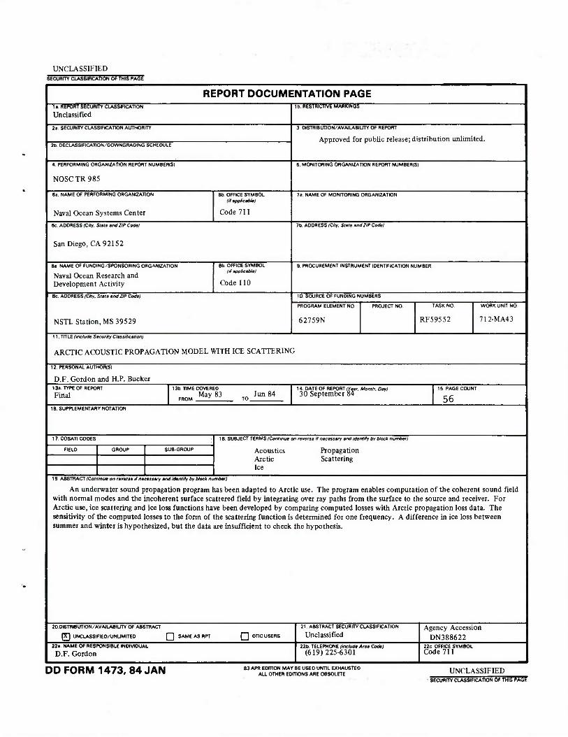
An underwater sound propagation program has been adapted to Arctic use. The program enables computation of the coherent sound field with normal modes and the incoherent surface scattered field by integrating over ray paths from the surface to the source and receiver. For Arctic use, ice scattering and ice loss functions have been developed by comparing computed losses with Arctic propagation loss data. The sensitivity of the computed losses to the form of the scattering function is determined for one frequency. A difference in ice loss between summer and winter is hypothesized, but the data are insufficient to check the hypothesis.

20 DISTRIBUTION/AVAILABILITY OF ABSTRACT

PT] UNCLASSIFIED/UNLIMITED ! "J SAME AS RPT £] DTIC USERS

21. ABSTRACT SECURITY CLASSIFICATION

Unclassified Agency Accession

DN388622 22« NAME Of RESPONSIBLE INDIVIDUAL

D.F. Gordon 22b TELEPHONE /include Aree Code)

(619)225-6301 22c OFFICE SYMBOL Code 711

DD FORM 1473, 84 JAN 83 APR EDITION MAY BE USED UNTIL EXHAUSTED ALL OTHER EDITIONS ARE OBSOLETE UNCLASSIFIED

SECURITY CLASSIFICATION OF THIS PAGE

UNCLASSIFIED

SKCUmTY CLASSIFICATION OP THIS * AOC (Wkm Omm

DO FORM 1473, 84 JAN UNCLASSIFIED

SECURITY CLASSIFICATION OP TNIS PAGtfWIwn Datm Kmtm*4)

EXECUTIVE SUMMARY

OBJECTIVE

The objectives of this work were to (1 ) improve the prediction of underwater sound propagation in the Arctic Ocean by determining ice reflection and scattering losses, and (2) develop a computer model of Arctic sound propagation.

RESULTS

1. A propagation loss model has been developed for the Arctic Ocean that should be of significant value in predicting Arctic propagation performance.

2. Ice scattering losses have been determined empirically and have given good fits to three major Arctic propagation loss data sets.

3. Specifications were developed for gathering data that would distinguish between different theoretical scattering functions.

RECOMMENDATIONS

1. Introduce relative phase into scattered sound fields so that accurately modeled array performance predictions can be made.

2. Gather under-ice propagation data that will facilitate scattering deter- mination. This requires closely spaced ranges in the first 60 km with sources or receivers spaced from above 50 m to below 400 m in depth and frequencies up to 500 Hz.

3. Use propagation loss data as they become available to update ice scattering curves used in this Arctic propagation model. Seasonal or ice condition dependence is needed.

4. Set limits on the ice scattering kernel by comparing computed losses with data.

CONTENTS

INTRODUCTION . . . page 1

DESCRIPTION OF THE ARCTIC PROPAGATION MODEL ... 3

ICE REFLECTION LOSS DETERMINATION ... 7

REFLECTION LOSS CURVES ... 7 ICE ATTENUATION LOSS ... 7 BOTTOM REFLECTIONS ... 9 ICE ROUGHNESS DEPENDENCE ... 9

FITTING PROPAGATION LOSS DATA ... 13

DIACHOK'S DATA ... 13 BUCK'S DATA ... 15 MELLEN AND MARSH DATA ... 15 ICE ROUGHNESS ... 1 5

COMPARISON OF REFLECTION LOSS FUNCTIONS ... 21

PROPAGATION LOSS FOR DIFFERENT SCATTERING FUNCTIONS ... 21 DIFFERENCE IN SUMMER AND WINTER COMPUTATIONS ... 24 REFLECTION LOSSES FOR MODELS WITH FIRST ORDER SCATTERING ... 24

CONCLUSION ... 28

REFERENCES ... 29

APPENDIX A: SAMPLE RUNS . . . A-1

11

ILLUSTRATIONS

4 5

10

1 1

12

13

14

15

16

17

18 19

20 21

22

23

24

Mode-to-ray and ray-to-mode conversion . . . page 3 Ray paths from mode m to the receiver ... 5 Ice reflection losses as a function of grazing angle at two freguencies as

used in the Arctic propagation program. The losses are due to scatter- ing except that part over the shaded area, which is due to ice loss ... 8

Slope of ice reflection loss curves as a function of freguency ... 8 Bottom reflection loss as a function of bottom grazing angle for four freguencies ... 10

Contours of standard deviation of ice depth in meters from LeSchack and Chang ... 11

Slope of ice scattering loss curves as a function of frequency and of s, the standard deviation of ice roughness ... 12

A five-layer approximation to a typical Arctic sound speed

profile ... 13 Comparison of Arctic shot data at 50 Hz with computed propagation losses.

Data from Diachok ... 14 Comparison of Arctic shot data at 200 Hz with computed propagation losses.

Data from Diachok ... 14 Comparison of Arctic shot and cw data at 50 Hz with computed propagation

16 cw data at 16

cw data at 17 at 100 Hz with computed propagation losses. . . 18 at 200 Hz with computed propagation losses. . . 18 at 800 Hz with computed propagation losses. . . 18

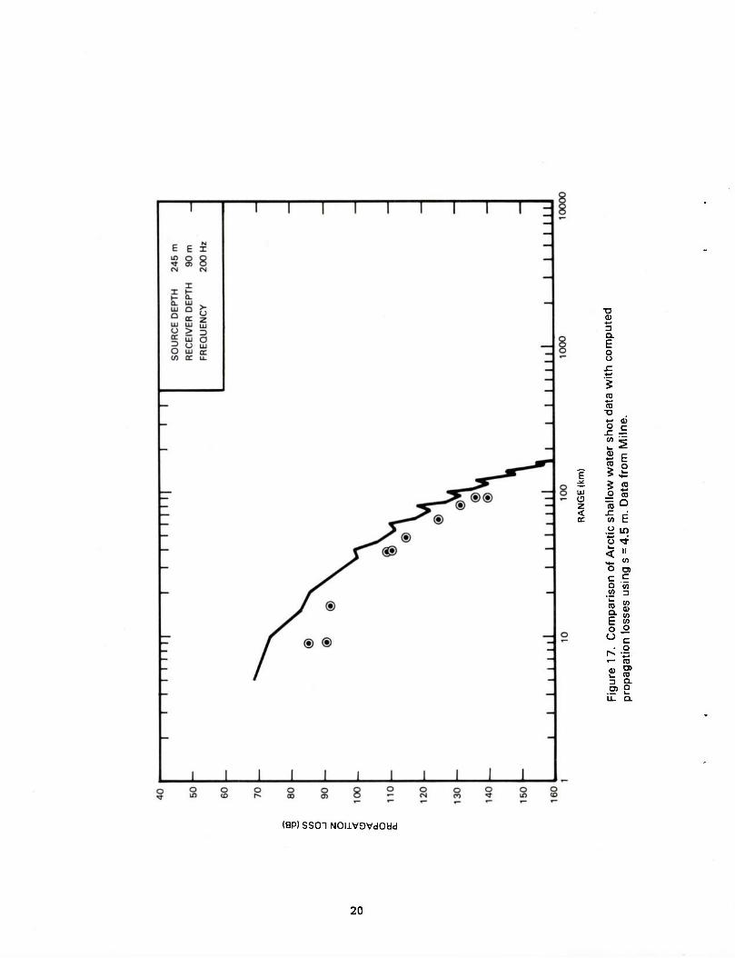
Comparison of Arctic shallow water shot data with computed propagation losses using s = 4.5 m. Data from Milne ... 20

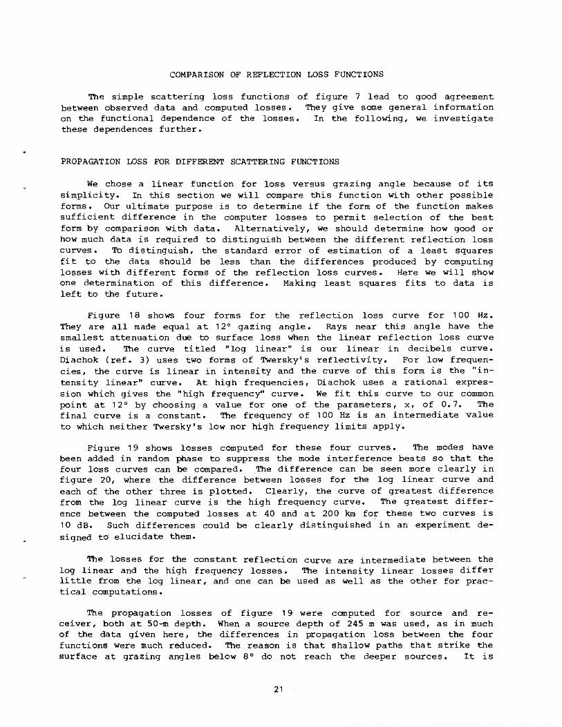
Four candidate reflection loss curves ... 22 Losses computed for the four reflection loss curves of Figure 18 at

100 Hz . . . 22 Differences between the loss curves of Figure 19 . . .22 The depth at which rays of given surface grazing angle vertex for the Arctic profile of Figure 8. The ray is confined between this depth and the surface ... 23

Difference between propagation loss computations with the ice loss curve starting at 13°, 15°, and 20° grazing angle ... 25

Comparison of propagation losses computed with and without secondary scattering ... 25

Propagation losses at two ranges and three receiver depths computed with and without secondary scattering ... 27

losses. Data from Buck . . Comparison of Arctic shot and

losses. Data from Buck . . Comparison of Arctic shot and

losses. Data from Buck . . Comparison of Arctic shot data

Data from Meilen and Marsh Comparison of Arctic shot data

Data from Meilen and Marsh Comparison of Arctic shot data

Data from Meilen and Marsh

100 Hz with computed propagation

200 Hz with computed propagation

ill

INTRODUCTION

In the Arctic Ocean, if one wishes to compute underwater sound propagation losses or to create a propagation loss model, the paramount problem is determining the effect of the overhead ice on the sound. Other aspects of sound propagation are generally easier to compute in the Arctic than in other ocean basins due to the stability of the sound speed profile and the dominance of the upward refracted, surface reflected propagation path. The acoustic effects of the ice are extremely complicated. The rough and irregular shape of the ice, its elastic properties, inhomogeneities, and even its snow cover, all affect the sound. These acoustic effects, including the parameters of the ice itself, are being ably and energetically investigated. However, while these studies are in progress, a best-available acoustic de- scription of the ice is needed. This description can be in the form of re- flection and scattering losses and scattering directions as functions of the appropriate variables. A knowledge of which variables are important is also needed.

The primary purpose of the effort reported here was to develop an acous- tic description of the ice as outlined above. Our strategy was to model the non-ice dependent aspects of sound propagation as well as possible. We then sought ice reflection values that gave the best fit between computed and observed propagation loss. The results provide good general levels of ice reflection loss as functions of grazing angle, frequency, and ice roughness. Other, less definitive results that may require more data to determine or substantiate involve the functional dependence or shape of the reflection loss for the above parameters, the directional characteristics of the non-specular scatter, seasonal dependence, and ice loss as opposed to ice scatter.

A second product of this effort is an Arctic propagation loss model. This model with our ice scattering losses incorporated into it agrees well with all three major sets of data used. Samples from each set are given in this report. We chose a normal mode model that was reliable and easy to use, though necessarily range independent. That is, we must assume the environment is constant in range. The result is an Arctic model that a user can apply with ease and confidence. It can be used in both deep and shallow water, with or without ice cover. The model is discussed in the first section of this report and the input-output for two runs are given in appendix A as an aid to users in constructing runs.

Because we were interested in ice scattering effects, we chose a model with both primary and secondary scattering. Primary scattering is the loss of energy at the surface due to scattering. Secondary scattering is the propaga- tion of this scattered energy to the source and receiver. A simple Arctic model with empirical ice loss could be constructed without using secondary scattering. However, one cannot hope to approach the true physics of the prob- lem without accounting for the scattered energy. The use of secondary scatter- ing in the model increases the acoustic parameters that need to be known, particularly the scattering directions or scattering kernel. It also greatly increases the information that the model can produce. The relative strength of the direct and scattered fields is an example. This is treated briefly in the final section of this report.

The scope of this study was limited by the propagation loss data that were available. For example, air-dropped explosive sources are by far the easiest sources to use in the Arctic. The data therefore tend to be sparse because the data can be gathered only from patches of open water. Also, the air drops cover long ranges; therefore the higher frequencies are greatly attenuated and tend to be neglected. We have therefore been most successful in estimating those ice acoustic effects that control the overall range dependent attenuation at frequencies of 200 Hz and below. Closely spaced and more detailed propagation loss data, when available, will permit better determination of other aspects of ice acoustics.

DESCRIPTION OF THE ARCTIC PROPAGATION MODEL

The Arctic sound field is presented as having two interacting components. There is a coherent sound field that is represented by a finite set of normal

modes and a stochastic component associated with the scattered field. The normal modes are an exact solution of the wave equation when the water-ice boundary does not scatter (i.e., at very low frequencies). The number of normal modes required is a linear function of frequency with as few as 110 normal modes needed at a frequency of 100 Hz for a typical Arctic profile for long ranges .

The stochastic component of the sound field is represented by a set of integrals that are the result of sound waves interacting with the rough water- ice boundary. The scattering integrals are associated with ray paths that direct sound energy from the source to the water-ice boundary or from the boundary to a receiver (hydrophone).

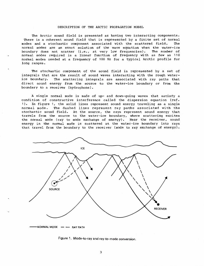
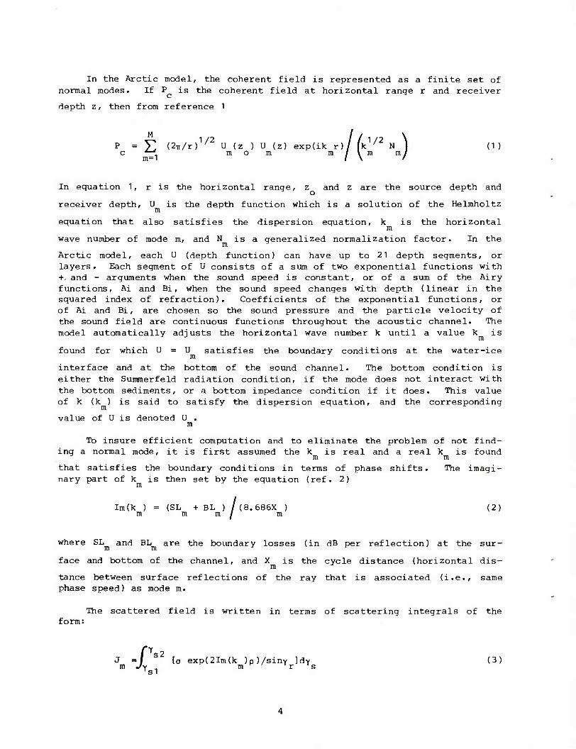
A single normal mode is made of up- and down-going waves that satisfy a condition of constructive interference called the dispersion equation (ref. 1 ). In figure 1, the solid lines represent sound energy traveling as a single normal mode. The dashed lines represent ray paths associated with the stochastic sound field. At the source, the rays represent sound energy that travels from the source to the water-ice boundary, where scattering excites the normal mode (ray to mode exchange of energy). Near the receiver, sound energy in the normal mode is scattered at the water-ice boundary into rays that travel from the boundary to the receiver (mode to ray exchange of energy).

-NORMAL MODE RAY PATH

Figure 1. Mode-to-ray and ray-to-mode conversion.

In the Arctic model, the coherent field is represented as a finite set of il modes. If P is the cc

c depth z, then from reference 1

normal modes. If P is the coherent field at horizontal range r and receiver c

P : Y, (2Tr/r)1/2 U (z ) U (z) exptik r)/ l\ /2 N J (1 ) / i m m / c *r, mom m

m=1

In equation 1, r is the horizontal range, z and z are the source depth and

receiver depth, U is the depth function which is a solution of the Helmholtz m

equation that also satisfies the dispersion equation, k is the horizontal m

wave number of mode m, and N is a generalized normalization factor. In the m *

Arctic model, each U (depth function) can have up to 21 depth segments, or layers. Each segment of U consists of a sum of two exponential functions with +. and - arguments when the sound speed is constant, or of a sum of the Airy functions, Ai and Bi, when the sound speed changes with depth (linear in the squared index of refraction). Coefficients of the exponential functions, or of Ai and Bi, are chosen so the sound pressure and the particle velocity of the sound field are continuous functions throughout the acoustic channel. The model automatically adjusts the horizontal wave number k until a value k is

found for which U = U satisfies the boundary conditions at the water-ice m

interface and at the bottom of the sound channel. The bottom condition is either the Summerfeld radiation condition, if the mode does not interact with the bottom sediments, or a bottom impedance condition if it does. This value of k (k ) is said to satisfy the dispersion equation, and the corresponding

value of U is denoted U . m

To insure efficient computation and to eliminate the problem of not find- ing a normal mode, it is first assumed the k is real and a real k is found m m that satisfies the boundary conditions in terms of phase shifts. The imagi- nary part of k is then set by the equation (ref. 2)

m

/ Im(k ) = (SL + BL ) /(8.686X ) (2)

m mm/ m

where SL and BL are the boundary losses (in dB per reflection) at the sur- m m

face and bottom of the channel, and X is the cycle distance (horizontal dis- m

tance between surface reflections of the ray that is associated (i.e., same phase speed) as mode m.

The scattered field is written in terms of scattering integrals of the form:

J =/ S2 la exp(2Im(k )p)/sinY ]dv (3) m Jy . m ■ r ' s

'si

The reader should refer to reference 1 for derivation of equation 3 and for the equations that relate equation 3 to the stochastic sound field. Here, we shall show the physical interpretation of equation 3 and indicate how the integral is calculated. In equation 3, y is the grazing angle of ray sound

energy at the water-ice boundary, y and y are the limiting values of rays

that can travel from the interface to the receiver, a is the scattering coeffi- cient, Y is the angle of the ray at the receiver, and P is the horizontal

distance from the point where the ray is scattered at the surface to the re- ceiver. There is also a related integral where the source replaces the receiver.

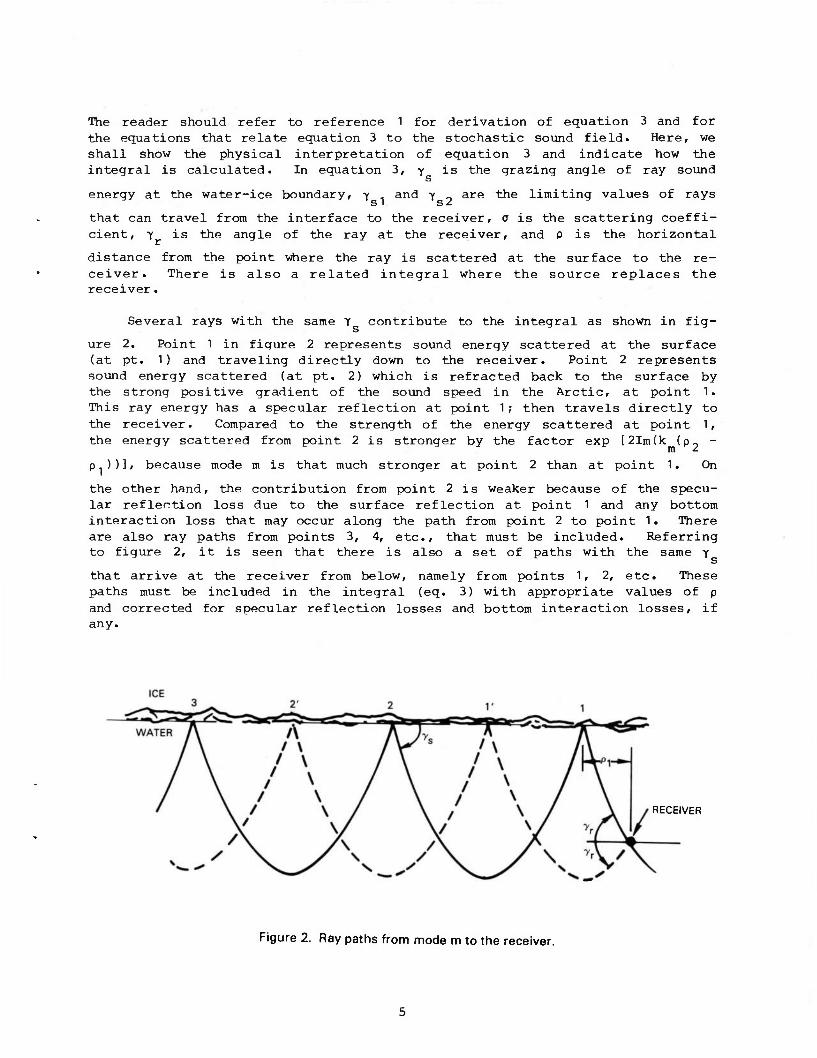
Several rays with the same Y contribute to the integral as shown in fig-

ure 2. Point 1 in figure 2 represents sound energy scattered at the surface (at pt. 1) and traveling directly down to the receiver. Point 2 represents sound energy scattered (at pt. 2) which is refracted back to the surface by the strong positive gradient of the sound speed in the Arctic, at point 1. This ray energy has a specular reflection at point 1 ; then travels directly to the receiver. Compared to the strength of the energy scattered at point 1, the energy scattered from point 2 is stronger by the factor exp [2Im(k (p -

m £

p.))]» because mode m is that much stronger at point 2 than at point 1. On

the other hand, the contribution from point 2 is weaker because of the specu- lar reflection loss due to the surface reflection at point 1 and any bottom interaction loss that may occur along the path from point 2 to point 1. There are also ray paths from points 3, 4, etc., that must be included. Referring to figure 2, it is seen that there is also a set of paths with the same y

that arrive at the receiver from below, namely from points 1, 2, etc. These paths must be included in the integral (eq. 3) with appropriate values of p and corrected for specular reflection losses and bottom interaction losses, if any.

RECEIVER

Figure 2. Ray paths from mode m to the receiver.

The scattering coefficient o depends on the angle of the mode (or the ray of the same wave number) at the surface, the scattering angle y , and the sur

face scattering loss. This is generally termed the scattering kernel. At present, the program uses a proportional to sin y , or Lambert scattering.

The mode angle enters only in determining the total energy scattered per re- flection. Only scattering in the forward direction is used. In future work we plan to determine the sensitivity of the computer propagation loss to these assumptions regarding the scattering kernel.

In summary for this section, the sound field is represented as two over- lapping fields. Thus, at any point in the channel, there will be a coherent field represented by a finite set of normal modes and a stochastic field con- sisting of a set of scattering integrals that are associated with ray paths from the source to the water-ice interface or from the interface to the re- ceiver. If the water-ice boundary is smooth, (i.e., r.m.s.- variations of the water-ice interface << X, where X is the acoustic wavelength), then a in equation 3 will approach zero and only the coherent field will be observable. As the frequency of the sound increases, there will be more scattering and a larger stochastic contribution to that total field. On the basis of our

limited experience, the Arctic model indicates an increasing stochastic field with frequency until saturation occurs, when the energy is about evenly di- vided between the stochastic and coherent sound fields.

ICE REFLECTION LOSS DETERMINATION

The purpose of the work reported in this section was to determine ice re- flection losses due both to scattering and attenuation. The scattering is due to irregularities at the ice-water interface. The attenuation is energy that is lost at reflection and does not re-enter the water. Much of it may be by absorption of various waves in the ice. Our strategy was to use the propaga- tion loss program described above to account for as many propagation parame- ters as possible. The principal unknowns are then the reflection losses. By comparing computed losses with observed losses, the reflection losses can be adjusted to give the best comparison. In this section we give the reflection loss curves that resulted from our investigation, a discussion of the data used, and finally, a discussion of the limitations that appear to be inherent in this method of determining coefficients.

REFLECTION LOSS CURVES

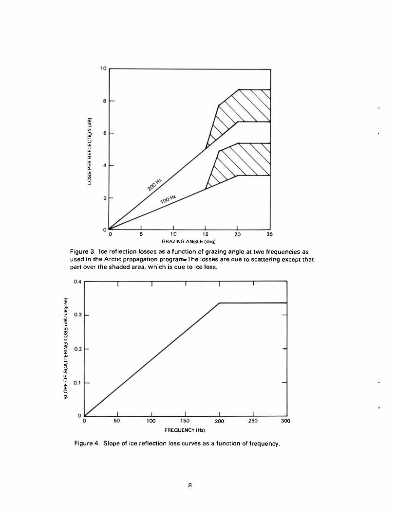
Figure 3 shows the reflection loss curves for two frequencies: 100 and 200 Hz. These curves give loss versus grazing angle for angles up to 20°. The curves over the shaded areas represent the reflection loss due to ice attenuation. The remainder of the loss represents scattering loss. This scattering loss is linear in decibel units for grazing angles up to 20°. The loss is 0 dB at 0° grazing angle. The scattering loss at any frequency is thus a curve of one parameter. A convenient way to express this parameter is the slope of the curve in dB/degree.

This slope of the scattering curve is a function of frequency. Figure 4 shows the frequency dependence of the slope. Note that the curve is flat above 200 Hz; i.e., the slope of the scattering loss is approximately 0.33 dB/degree for all frequencies above 200 Hz. This effect is apparently due to the scattering objects (the ice keels) becoming large compared to an acoustic wavelength. Diachok (ref. 3) demonstrates this effect and explains it using Twersky's loss scattering model. These scattering losses are determined for data from the central Arctic deep water areas. Corrections for other ice conditions will be discussed later.

ICE ATTENUATION LOSS

In figure 3, the difference between the losses caused by ice attenuation and those caused by scattering are represented by the shaded area. The ice- loss curve increases from 0 to 2 dB above the scattering curve over a 2° interval, and then remains at 2 dB above the scattering curve. These values are independent of frequency. Here, this additional reflection loss starts at 15° grazing angle. We use this value for winter ice. For summer ice we lower the starting angle to 13°. This is the only seasonal difference that we use in our reflection coefficients, and is a purely hypothetical difference. As will be shown later, it makes only a small difference in propagation loss, and very accurate data will be needed to test it. Differences in roughness of summer and winter ice may well overshadow the effect.

CQ

Z o o

oc LU Q.

CO co O

20 25 0 5 10 15

GRAZING ANGLE (deg)

Figure 3. Ice reflection losses as a function of grazing angle at two frequencies as used in the Arctic propagation program*The losses are due to scattering except that part over the shaded area, which is due to ice loss.

Q) ■D \ m ;o

V) CO o o cr LU

< u CO

u- o a. O

100 150

FREQUENCY (Hz)

200 300

Figure 4. Slope of ice reflection loss curves as a function of frequency.

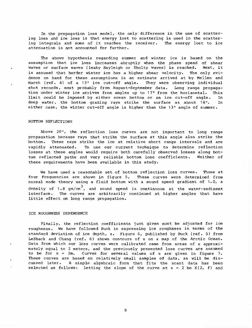
In the propagation loss model, the only difference in the use of scatter- ing loss and ice loss is that energy lost to scattering is used in the scatter- ing integrals and some of it reaches the receiver. The energy lost to ice attenuation is not accounted for further.

The above hypothesis regarding summer and winter ice is based on the assumption that ice loss increases abruptly when the phase speed of shear waves or surface waves (leaky Rayleigh or Sholty waves) is reached. Next, it is assumed that harder winter ice has a higher shear velocity. The only evi- dence on hand for these assumptions is an estimate arrived at by Meilen and Marsh (ref. 4) of a 13° ice cut-off angle. They were observing individual shot records, most probably from August-September data. Long range propaga- tion under winter ice arrives from angles up to 17° from the horizontal. This limit could be imposed by either ocean bottom or an ice cut-off angle. In deep water, the bottom grazing rays strike the surface at about 18°. In either case, the winter cut-off angle is higher than the 13° angle of summer.

BOTTOM REFLECTIONS

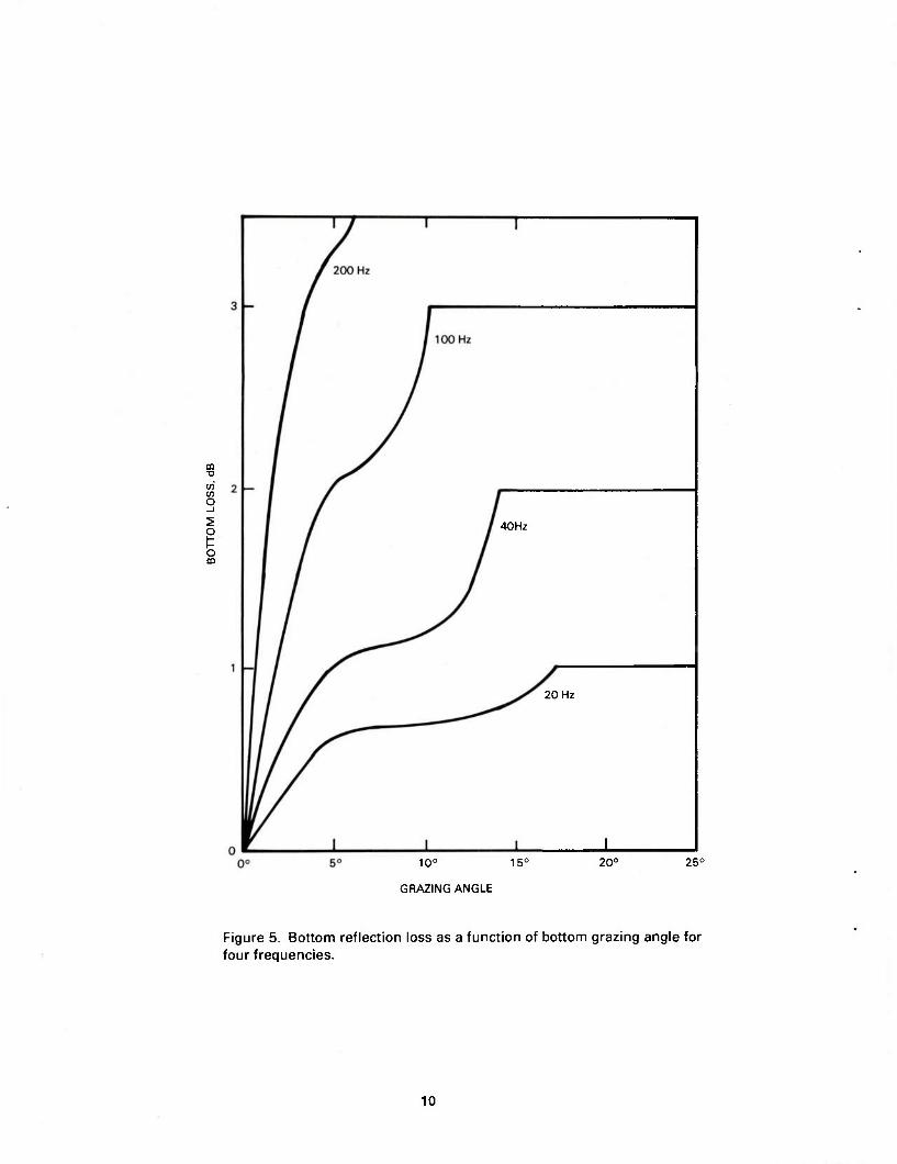
Above 20°, the reflection loss curves are not important to long range propagation because rays that strike the surface at this angle also strike the bottom. These rays strike the ice at relative short range intervals and are rapidly attenuated. To use our current technique to determine reflection losses at these angles would require both carefully observed losses along bot- tom reflected paths and very reliable bottom loss coefficients. Neither of these requirements have been available in this study.

We have used a reasonable set of bottom reflection loss curves. Those at four frequencies are shown in figure 5. These curves were determined from normal mode theory using a fluid bottom with a sound speed gradient of 1.0, a

density of 1.8 gm/cm , and sound speed is continuous at the water-sediment interface. The curves are arbitrarily continued at higher angles that have little effect on long range propagation.

ICE ROUGHNESS DEPENDENCE

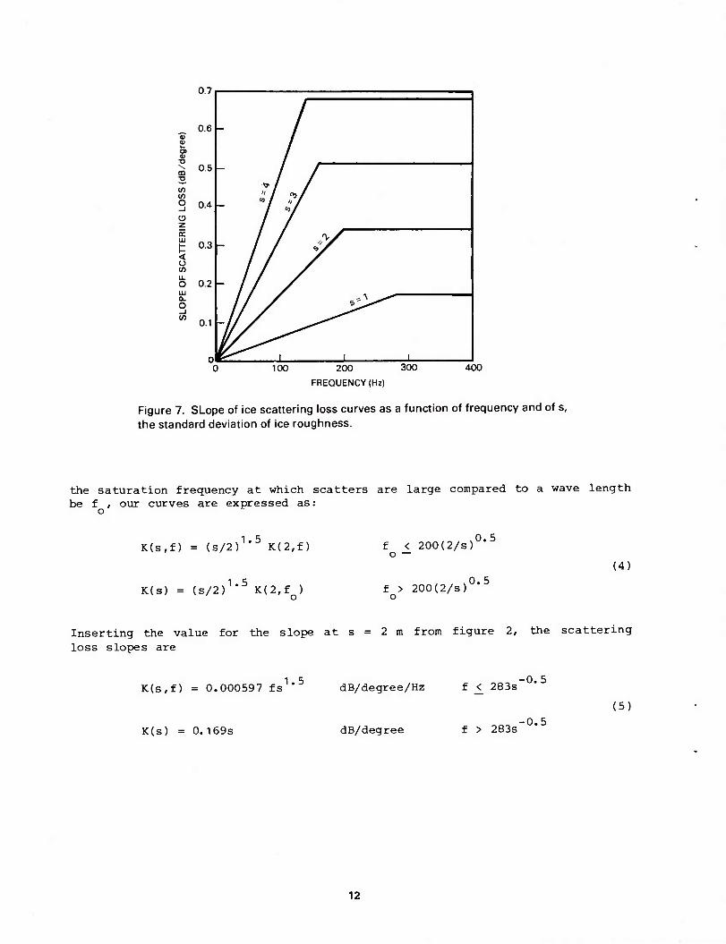
Finally, the reflection coefficients just given must be adjusted for ice roughness. We have followed Buck in expressing ice roughness in terms of the standard deviation of ice depth, s. Figure 6, published by Buck (ref. 5) from LeShack and Chang (ref. 6) shows contours of s on a map of the Arctic Ocean. Data from which our loss curves were calibrated came from areas of s approxi- mately equal to 2 meters, and the previously presented loss curves are assumed to be for s = 2m. Curves for several values of s are given in figure 7. These curves are based on relatively small samples of data, as will be dis- cussed later. A simple algebraic form that fits the scant data has been selected as follows: letting the slope of the curve at s = 2 be K(2, f) and

CQ

<s> O _i

o

o m

40Hz

20 Hz

10° 15°

GRAZING ANGLE

20° 25°

Figure 5. Bottom reflection loss as a function of bottom grazing angle for four frequencies.

10

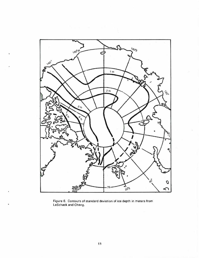
Figure 6. Contours of standard deviation of ice depth in meters from LeSchack and Chang.

11

v. /

0.6 a) 0)

CT ID -o

0.5 CO T3

V i CO to " / "j/ o 0.4 -

69 / // /

o z

0.3 _ LU

< o to

o 0.2 LLI 0- o s ^^^^ _l CO

0.1

0 I 1 1 100 200 300

FREQUENCY (Hz)

400

Figure 7. SLope of ice scattering loss curves as a function of frequency and of s, the standard deviation of ice roughness.

the saturation frequency at which scatters are large compared to a wave length be f , our curves are expressed as:

o

K(s,f) = (s/2)1'5 K(2,f)

K(s) = (s/2)1*5 K(2,fQ)

f < 200(2/s) o —

0.5

(4)

f > 200(2/s) o

0.5

Inserting the value for the slope at s = 2 m from figure 2, the scattering loss slopes are

K(s,f) = 0.000597 fs dB/degree/Hz f <_ 283s~

(5)

K(s) = 0.169s dB/degree f > 283s -0.5

12

FITTING PROPAGATION LOSS DATA

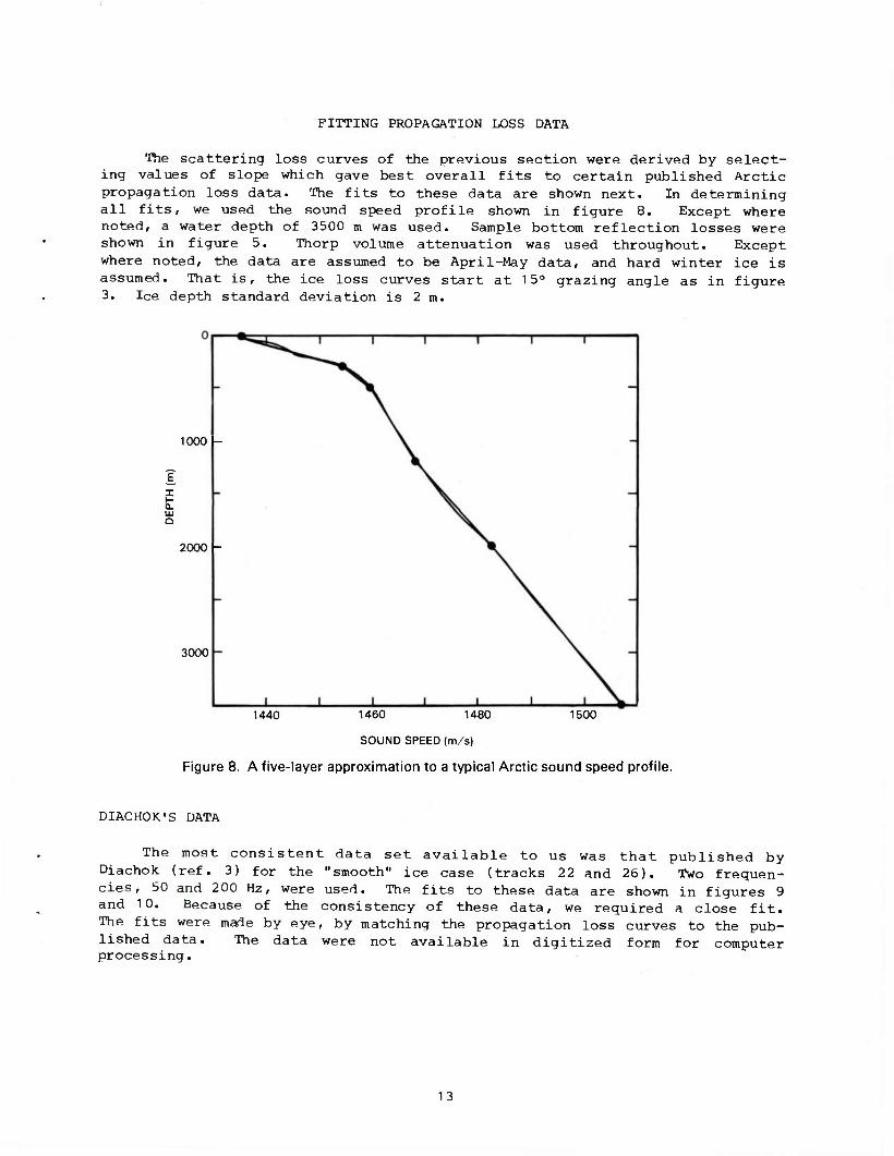
The scattering loss curves of the previous section were derived by select- ing values of slope which gave best overall fits to certain published Arctic propagation loss data. The fits to these data are shown next. In determining all fits, we used the sound speed profile shown in figure 8. Except where noted, a water depth of 3500 m was used. Sample bottom reflection losses were shown in figure 5. Thorp volume attenuation was used throughout. Except where noted, the data are assumed to be April-May data, and hard winter ice is assumed. That is, the ice loss curves start at 15° grazing angle as in figure 3. Ice depth standard deviation is 2 m.

1000 -

x t LU Q

2000 -

3000

1440 1500 1460 1480

SOUND SPEED (m/s)

Figure 8. A five-layer approximation to a typical Arctic sound speed profile.

DIACHOK'S DATA

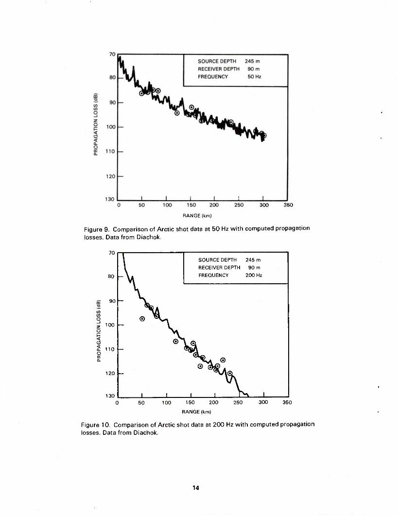
The most consistent data set available to us was that published by Diachok (ref. 3) for the "smooth" ice case (tracks 2 2 and 26). Two frequen- cies, 50 and 200 Hz, were used. The fits to these data are shown in figures 9 and 10. Because of the consistency of these data, we required a close fit. The fits were made by eye, by matching the propagation loss curves to the pub- lished data. The data were not available in digitized form for computer processing.

13

300 350

RANGE (km)

Figure 9. Comparison of Arctic shot data at 50 Hz with computed propagation losses. Data from Diachok.

CO

to CO

O _i 2 o F < < a. o ca CL

/o SOURCE DEPTH 245 m RECEIVER DEPTH 90 m

80 FREQUENCY 200 Hz

90

100 © ^

© \ (•) 110

VA © © <&©

120 ^^^i(SL

130 I 1 i i r W 1 50 100 150 200

RANGE (km)

250 300 350

Figure 10. Comparison of Arctic shot data at 200 Hz with computed propagation losses. Data from Diachok.

14

BUCK'S DATA

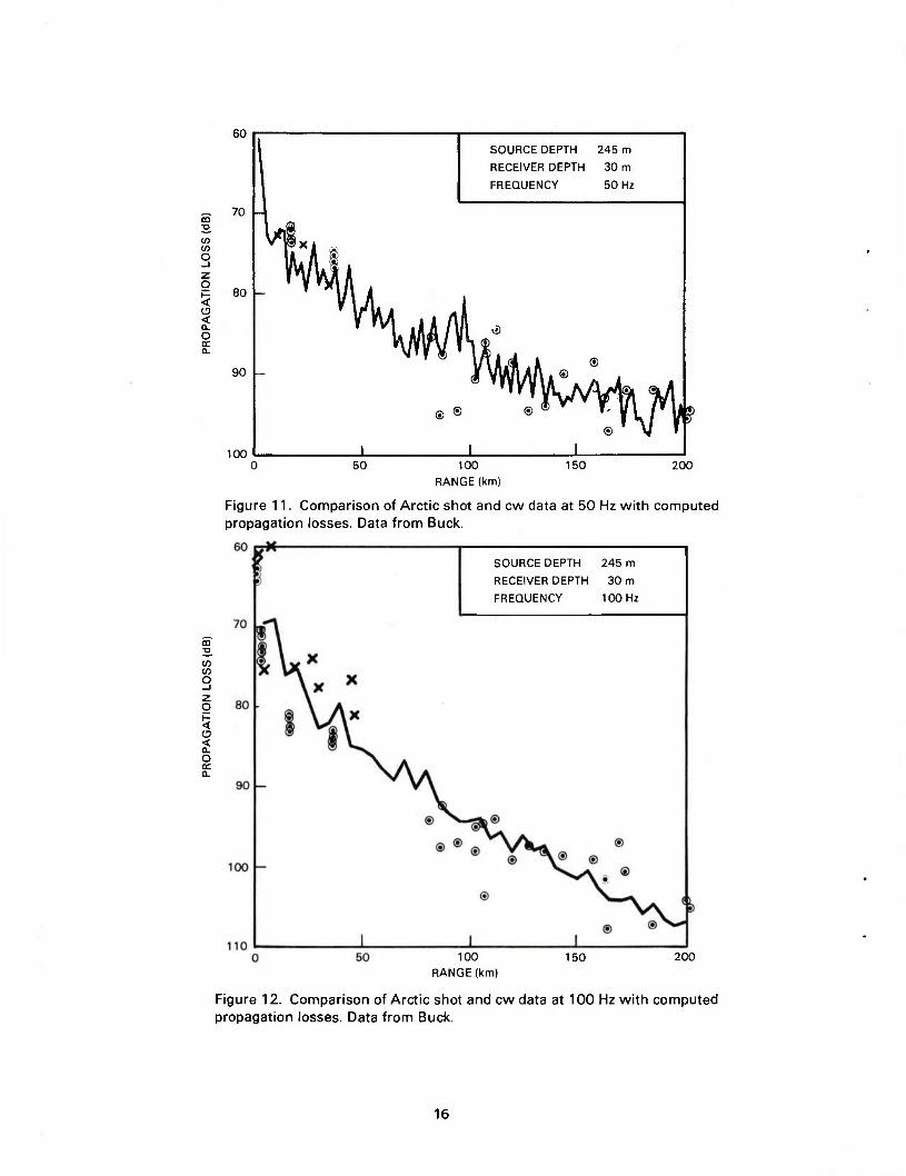
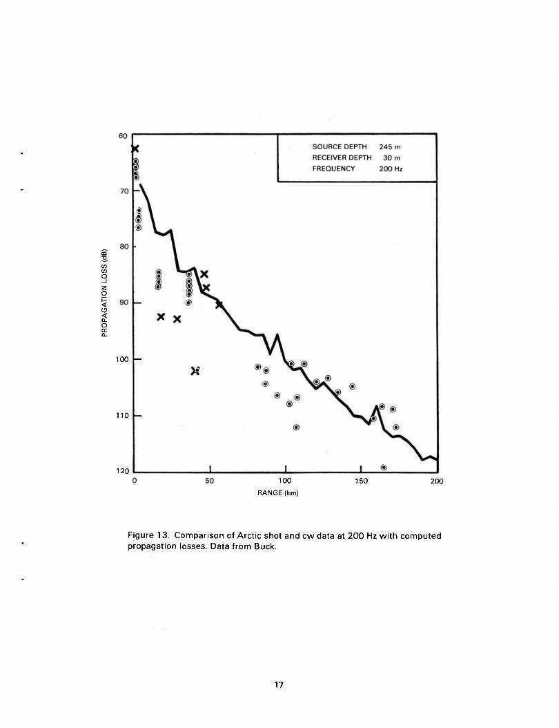
Data published by Buck (ref. 5) were apparently derived from more diverse observations, but were for a single shot depth and a single receiver depth, as printed on the figures. Buck states that data for shallow paths have been excluded from the set. The data include frequencies from 10 to 200 Hz. Fig- ures 11 to 13 show fits for 50, 100, and 200 Hz. The computed losses differ from those of the previous figures only in receiver depth. The circles in the figures represent shot data and the crosses are from cw data.

In these three plots, there is a tendency for the computed losses to be above the data at intermediate ranges and below the data at longer ranges. This may indicate a shortcoming in our reflection loss curve, which is linear in decibels. This will be discussed later. However, this interpretation is not compelling, and a simple scatter of the data is also a possible inter- pretation.

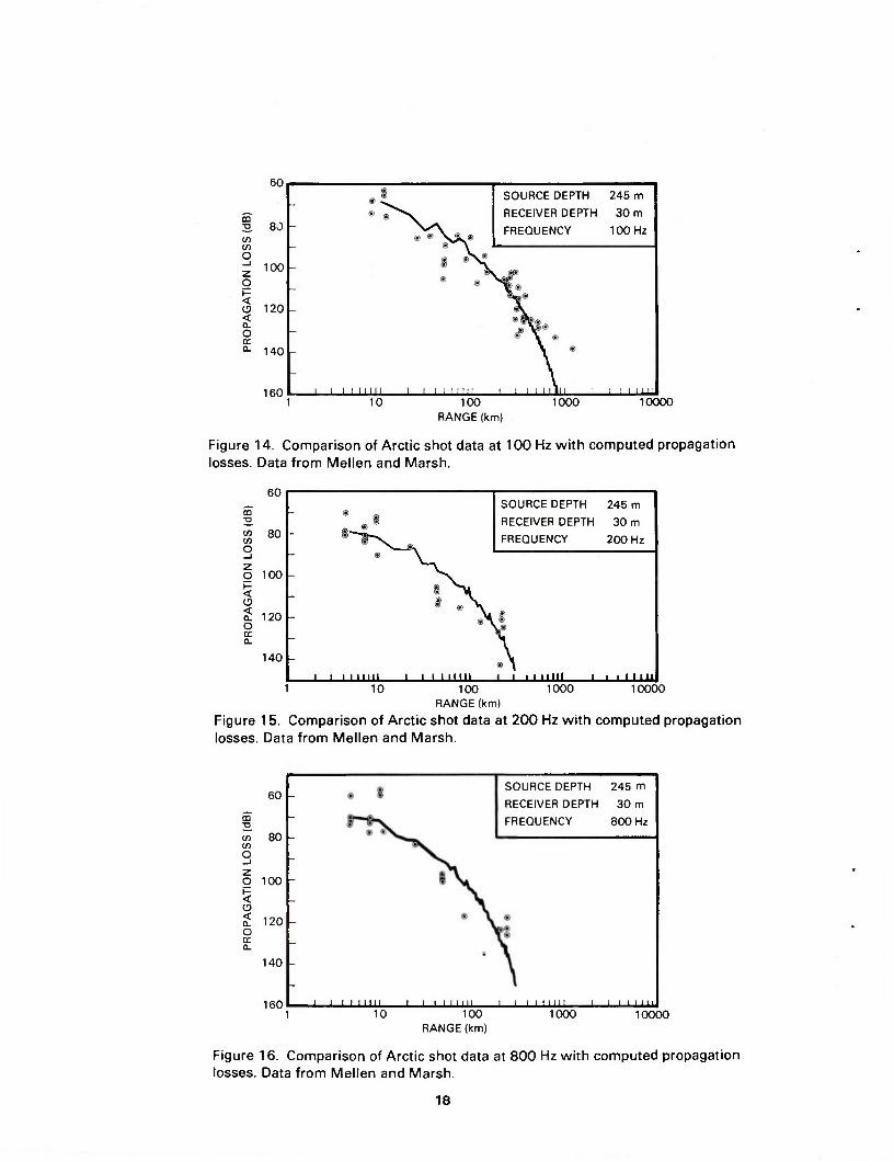
MELLEN AND MARSH DATA

The third set of data available to us was that of Meilen and Marsh (ref. 4). These data were taken predominantly in 1959 and 1962 from Fletcher's Ice Island (T3) and are of a more varied nature than the previous sets. Source depth, receiver depth, and shot yields varied. The presence of the ice island at the receiver may have introduced a consistent increase in loss into the data. This ice island might also have been the source of the 13° ice cut-off angle that we have attributed to summer ice. The greatest source of variation in the loss data is almost certainly the ocean depth. The ice island was in water of less than 1000-m depth when much of the data were gathered. Assuming that shallow water along the propagation path is more likely to increase loss than to decrease it, we have chosen to fit our loss curves to the less lossy data points.

Figures 14 to 16 show fits to the Meilen and Marsh data at frequencies of 100, 200, and 800 Hz. These data are particularly useful in giving us some higher frequency points to tie down the high frequency end of the reflection loss curves.

ICE ROUGHNESS

The ice roughness dependence of our reflection loss function was deter- mined with considerably less precision than the frequency dependence. This is because fewer data sets were available, and also because knowledge of s (the ice depth standard deviation) to attribute to the data sets was far from cer- tain. The following data were employed. Diachok's (ref. 3) "rough" ice cases (tracks 18 and 20) were used with s = 3.5 m. Buck's empirical fit gave a good functional relationship between s and propagation loss for frequencies between 10 and 100 Hz. Finally, Milne's (ref. 7) data were tried. These last data were of little real value to us because the experimental track extends from water of 500- to 1300-m depth. Our constant depth model cannot be used with confidence for such a path. Nevertheless, a computation using a depth of 700 m and s = 4.5 m showed good agreement with the slope of the data at 100 Hz.

15

CO T3

CO to o _l

z g \ < a. o cc 0.

60

70 CD

en O

p 80 - < < O- O cc Q-

90 -

100

SOURCE DEPTH 245 m

RECEIVER DEPTH 30 m

FREQUENCY 50 Hz

-

pxi 1

IL *

- <$ VWI/AA ® ®

/4 y»l®i ®i A

® ® ® * V \ / u ® V *]

1 i i 50 100

RANGE (km) 150 200

Figure 11. Comparison of Arctic shot and cw data at 50 Hz with computed propagation losses. Data from Buck.

SOURCE DEPTH 245 m

RECEIVER DEPTH 30 m

FREQUENCY 100 Hz

100

RANGE (km)

Figure 12. Comparison of Arctic shot and cw data at 100 Hz with computed propagation losses. Data from Buck.

16

CO if) O _i

o < < a. O tr CL

100 —

110 —

120 100

RANGE (km)

150 200

Figure 13. Comparison of Arctic shot and cw data at 200 Hz with computed propagation losses. Data from Buck.

17

60

S 80 - co co o

100 -

O 120

o cc °- 140

160

- ® «

SOURCE DEPTH

RECEIVER DEPTH

245 m

30 m

® • X JL ® FREQUENCY 100 Hz

- f s\®

• ^g®

•V

- MV* • \ •

- \ *

I I I I LIU ! ! I ! I : i 1 Hill i ..... I ...

10 100 RANGE (km)

1000 10000

Figure 14. Comparison of Arctic shot data at 100 Hz with computed propagation losses. Data from Meilen and Marsh.

60

£ ■o

% 80 o

o 100

o £ 120 o tr 0-

140 -

1

• ^ SOURCE DEPTH 245 m

- - 8

® "\

RECEIVER DEPTH

FREQUENCY

30 m

200 Hz

- ® ®

_ ®A.® V

- ® " L 1 1 1 Mill 1 i i nun 1 1 11 Ulli 1 ■ 1 Mill

10 1000 10000 100 RANGE (km)

Figure 15. Comparison of Arctic shot data at 200 Hz with computed propagation losses. Data from Meilen and Marsh.

CD •O

CD CO

O

60

80

o loo < < a. o cr 0.

120

140

160 1 I I I I ""

SOURCE DEPTH 245 m

RECEIVER DEPTH 30 m

FREQUENCY 800 Hz

10 J I l l l I ill Ill ' "

100 RANGE (km)

1000 10000

Figure 16. Comparison of Arctic shot data at 800 Hz with computed propagation losses. Data from Meilen and Marsh.

18

Figure 17 shows the fit using the Milne data points as plotted by Meilen and Marsh (ref. 4).

The slope of the computed and observed losses agrees well, but there is a consistent 7-dB offset beyond the first two data points.

The above data represent a small number of points upon which to base the ice-roughness dependence of our curves. This dependence should therefore be considered tentative, pending the availability of more data. Of course, our overall strategy of determining reflection loss curves is data dependent. The curves are therefore expected to change as additional data are used to verify and update them.

19

E

LU a z < DC

-a ■»-•

■3 a.

o o

■a

Si 1 £

O CD

« Q

5 E « to 6 -* < jj O OJ c E O 03

.<2 3 en 6 Q. •

o o u c *{ f (D

a s?

Ü. Q.

(ap) SS01 NOUVOVdOHd

20

COMPARISON OF REFLECTION LOSS FUNCTIONS

The simple scattering loss functions of figure 7 lead to good agreement between observed data and computed losses. They give some general information on the functional dependence of the losses. In the following, we investigate these dependences further.

PROPAGATION LOSS FOR DIFFERENT SCATTERING FUNCTIONS

We chose a linear function for loss versus grazing angle because of its simplicity. In this section we will compare this function with other possible forms. Our ultimate purpose is to determine if the form of the function makes sufficient difference in the computer losses to permit selection of the best form by comparison with data. Alternatively, we should determine how good or how much data is required to distinguish between the different reflection loss curves. To distinguish, the standard error of estimation of a least squares fit to the data should be less than the differences produced by computing losses with different forms of the reflection loss curves. Here we will show one determination of this difference. Making least squares fits to data is left to the future.

Figure 18 shows four forms for the reflection loss curve for 100 Hz. They are all made equal at 12° gazing angle. Rays near this angle have the smallest attenuation due to surface loss when the linear reflection loss curve is used. The curve titled "log linear" is our linear in decibels curve. Diachok (ref. 3) uses two forms of Twersky's reflectivity. For low frequen- cies, the curve is linear in intensity and the curve of this form is the "in- tensity linear" curve. At high frequencies, Diachok uses a rational expres- sion which gives the "high frequency" curve. We fit this curve to our common point at 12° by choosing a value for one of the parameters, x, of 0.7. The final curve is a constant. The frequency of 100 Hz is an intermediate value to which neither Twersky's low nor high frequency limits apply.

Figure 19 shows losses computed for these four curves. The modes have been added in random phase to suppress the mode interference beats so that the four loss curves can be compared. The difference can be seen more clearly in figure 20, where the difference between losses for the log linear curve and each of the other three is plotted. Clearly, the curve of greatest difference from the log linear curve is the high frequency curve. The greatest differ- ence between the computed losses at 40 and at 200 km for these two curves is 10 dB. Such differences could be clearly distinguished in an experiment de- signed to elucidate them.

The losses for the constant reflection curve are intermediate between the log linear and the high frequency losses. The intensity linear losses differ little from the log linear, and one can be used as well as the other for prac- tical computations.

The propagation losses of figure 19 were computed for source and re- ceiver, both at 50-m depth. When a source depth of 245 m was used, as in much of the data given here, the differences in propagation loss between the four functions were much reduced. The reason is that shallow paths that strike the surface at grazing angles below 8° do not reach the deeper sources. It is

21

DC cc w CL

in o

8 12 16 20 24

GRAZING ANGLE (deg)

Figure 18. Four candidate reflection loss curves.

60

70

8 80

< S3 <

100

110

120

1\ ,L0G LINEAR

\V^ ^ INTENSITY LINEAR

SÄ

HIGH FREQUENCY V

^X ^CONSTANT

100 200 300 400 500

RANGE (km)

Figure 19. Losses computed for the four reflection loss curves of Figure 18 at 100 Hz.

1/5 o -I Z g < < o. o cc a.

U z LU tr

4

it -8

X

/ CONSTANT *'

y / HIGH \> FREQUENCY

INTENSITY LINEAR

1 L .

0 100 200 300 400 500

RANGE (km)

Figure 20. Differences between the loss curves of Figure 19.

22

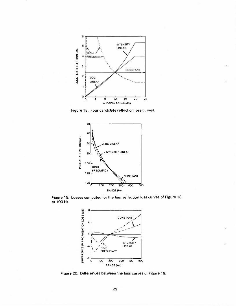
these paths where the different loss functions discriminate most. When these paths are not included, the discrimination between the different functions is lost. Figure 21 shows path depth or ray vertexing depth as a function of sur- face grazing angle for the Arctic profile used here. For a given source or receiver depth, rays with surface grazing angles less than that shown in the figure will pass above the source or receiver. Only diffracted or scattered energy from these shallower paths will be propagated.

This need for shallow source and receiver means that the data given here, such as that of figure 12, are not effective for distinguishing between dif- ferent scattering curves. It further indicates that an experiment designed to indicate something about the scattering curves should have a shallow source and receivers.

100 —

200 —

LU Q

u

>

500

300 —

400 —

SURFACE GRAZING ANGLE (deg)

Figure 21. The depth at which rays of given surface grazing angle vertex for the Arctic profile of Figure 8. The ray is confined between this depth and the surface.

23

DIFFERENCE IN SUMMER AND WINTER COMPUTATIONS

As stated earlier, this computer model distinguishes between winter and summer ice by placing the leading edge of a 2-dB ice loss function either at a 13° or 15° grazing angle. The ice loss was illustrated by the shaded area in figure 3. The ice loss was implemented in hopes that ice cut-off angles could be elucidated by comparing computer runs with observed data. In the follow- ing, we compare runs that differ only in this way and show that the difference is small. It appears that reliable values of ice loss will have to be deter- mined in other ways, and that their inclusion in the program will not greatly alter its output.

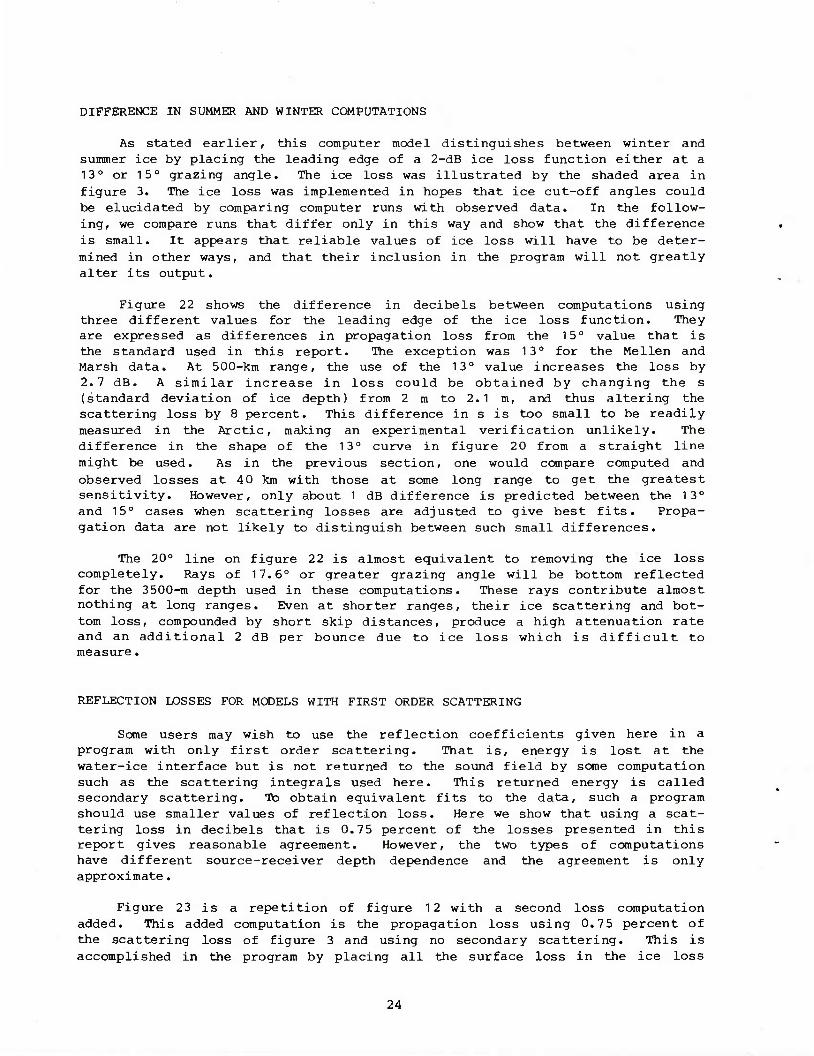
Figure 22 shows the difference in decibels between computations using three different values for the leading edge of the ice loss function. They are expressed as differences in propagation loss from the 15° value that is the standard used in this report. The exception was 13° for the Meilen and Marsh data. At 500-km range, the use of the 13° value increases the loss by 2.7 dB. A similar increase in loss could be obtained by changing the s (standard deviation of ice depth) from 2 m to 2.1 m, and thus altering the scattering loss by 8 percent. This difference in s is too small to be readily measured in the Arctic, making an experimental verification unlikely. The difference in the shape of the 13° curve in figure 20 from a straight line might be used. As in the previous section, one would compare computed and observed losses at 40 km with those at some long range to get the greatest sensitivity. However, only about 1 dB difference is predicted between the 13° and 15° cases when scattering losses are adjusted to give best fits. Propa- gation data are not likely to distinguish between such small differences.

The 20° line on figure 22 is almost equivalent to removing the ice loss completely. Rays of 17.6° or greater grazing angle will be bottom reflected for the 3500-m depth used in these computations. These rays contribute almost nothing at long ranges. Even at shorter ranges, their ice scattering and bot- tom loss, compounded by short skip distances, produce a high attenuation rate and an additional 2 dB per bounce due to ice loss which is difficult to measure.

REFLECTION LOSSES FOR MODELS WITH FIRST ORDER SCATTERING

Some users may wish to use the reflection coefficients given here in a program with only first order scattering. That is, energy is lost at the water-ice interface but is not returned to the sound field by some computation such as the scattering integrals used here. This returned energy is called secondary scattering. To obtain equivalent fits to the data, such a program should use smaller values of reflection loss. Here we show that using a scat- tering loss in decibels that is 0.75 percent of the losses presented in this report gives reasonable agreement. However, the two types of computations have different source-receiver depth dependence and the agreement is only approximate.

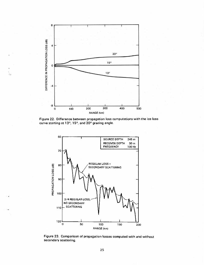
Figure 23 is a repetition of figure 12 with a second loss computation added. This added computation is the propagation loss using 0.75 percent of the scattering loss of figure 3 and using no secondary scattering. This is accomplished in the program by placing all the surface loss in the ice loss

24

...

100 200 300

RANGE (km)

400 500

Figure 22. Difference between propagation loss computations with the ice loss curve starting at 13°, 15°, and 20° grazing angle.

m ;o to 10 O

< < 0. o <r 0.

60

70 -

80 -

90 -

100-

110

120

I SOURCE DEPTH 245 m RECEIVER DEPTH 30 m FREQUENCY 100 Hz

^ —

_ y\ . , REGULAR LOSS + \V-A /SECONDARY SCATTERING

- v W 3/4 REGULAR LOSS, -""| I \\\~\^> NO SECONDARY U \ /wN'

_ SCATTERING W v\l \ A _

50 100

RANGE (km)

150 200

Figure 23. Comparison of propagation losses computed with and without secondary scattering.

25

table and none in the scattering loss table. The surface scattering integrals therefore make no contribution to the field. The most apparent difference between the two computations in figure 2 3 is the much greater fluctuation in the losses without secondary scattering. This is because the scattering inte- grals give a rather smooth loss function that fills in the interference nulls in the coherent mode results.

The source-receiver depth dependence of the computations with and without secondary scattering is complicated. We have not studied it in detail. Here we will point out one difference and show one comparison as an introduction to the topic.

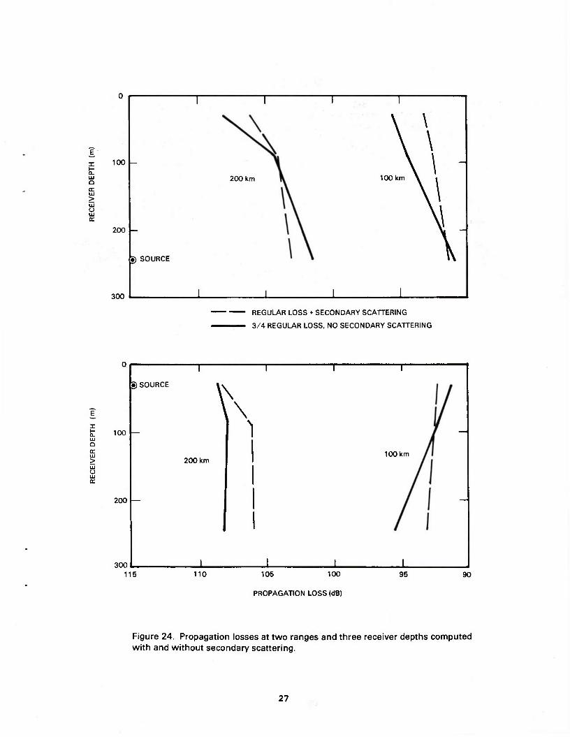
In the Arctic positive gradient sound speed profile, a deep source or receiver fails to intercept some rays which pass above it. If a shallow source is producing such rays, scattering can direct some energy from them down to a deeper receiver. By reciprocity, the same thing can happen for a deep source and shallow receiver. This produces a scattered field that is relatively strong compared to the direct field. Thus, when source and re- ceiver are at different depths, the computation with secondary scattering will show relatively less loss than that without secondary scattering. When source and receiver are near the same depth, this extra advantage is lost and losses computed without secondary scattering are relatively smaller.

The above effect is shown in figure 24. Random phase mode losses are shown for ranges of 100 and 200 km. In general, the losses with secondary scattering are greater when source and receiver are at the same depth and smaller when they are at different depths. The two computations are roughly egual, because of the reduction of the surface loss to 7 5 percent for the no secondary scatter case.

26

X F 0- LU Q

IT LU > LU CJ LU <r

100

200

300

9, SOURCE

200 km

I

100 km

REGULAR LOSS + SECONDARY SCATTERING

3/4 REGULAR LOSS, NO SECONDARY SCATTERING

DSOURCE

x F Q- LU o LU > LU U LU

100

200

300 L— 115

\

\

200 km

\

110 105 100

PROPAGATION LOSS (dB)

100 km

95 90

Figure 24. Propagation losses at two ranges and three receiver depths computed with and without secondary scattering.

27

CONCLUSION

A normal mode computer model has been adapted to Arctic underwater sound propagation. The model integrates over ray paths from the rough surface to the source and receiver to compute the scattered part of the sound field. Ice scattering losses have been determined, and with their use the model gives very good agreement with observed Arctic data. Ice attenuation loss is incor- porated in the model, but the data available are not sufficient to determine the small differences in propagation loss caused by ice attenuation.

Available propagation loss data do not permit evaluation of the exact functional dependence of scattering loss upon grazing angle. However, experi- mental configurations are discussed that would help determine the functional dependence.

It is shown that a program which does not use secondary scattering can obtain results approximating ours if an ice scattering loss of 75 percent of our loss in decibels is used. However, the source receiver dependence of the results cannot be made to coincide exactly.

28

REFERENCES

1. H.P. Bucker, "Wave Propagation in a Duct with Boundary Scattering (with application to a Surface Duct)," J. Acoust. Soc. Am. 68, 1768-1772 (1976).

2. H.P. Bucker, "Sound Propagation in a Channel with Lossy Boundaries," J. Acoust. Soc. Am. 48, 1187-1194 (1970).

3. 0.1. Diachok, "Effects of Sea-Ice Ridges on Sound Propagation in the Arctic Ocean," J. Acoust. Soc. Am. 59, 1110-1120 (1976).

4. R.H. Meilen and H.W. Marsh, "Underwater Sound in the Arctic Ocean," AVCO Marine Electronics Office Report MED-65-1002 (Aug 1965).

5. B.M. Buck, "Preliminary Under Ice Propagation Models Based on Synoptic Ice Roughness," Polar Research Lab TR-30 (May 1981).

6. L.A. LeSchack and D.C. Chang, "Arctic Under-Ice Roughness," Development and Resources Transportation Co. Tech. Rept. (1977).

7. A.R. Milne, "A 90 Km Sound Transmission Test in the Arctic," J. Acoust. Soc. Am. 35, 1459-1461 (1963).

29

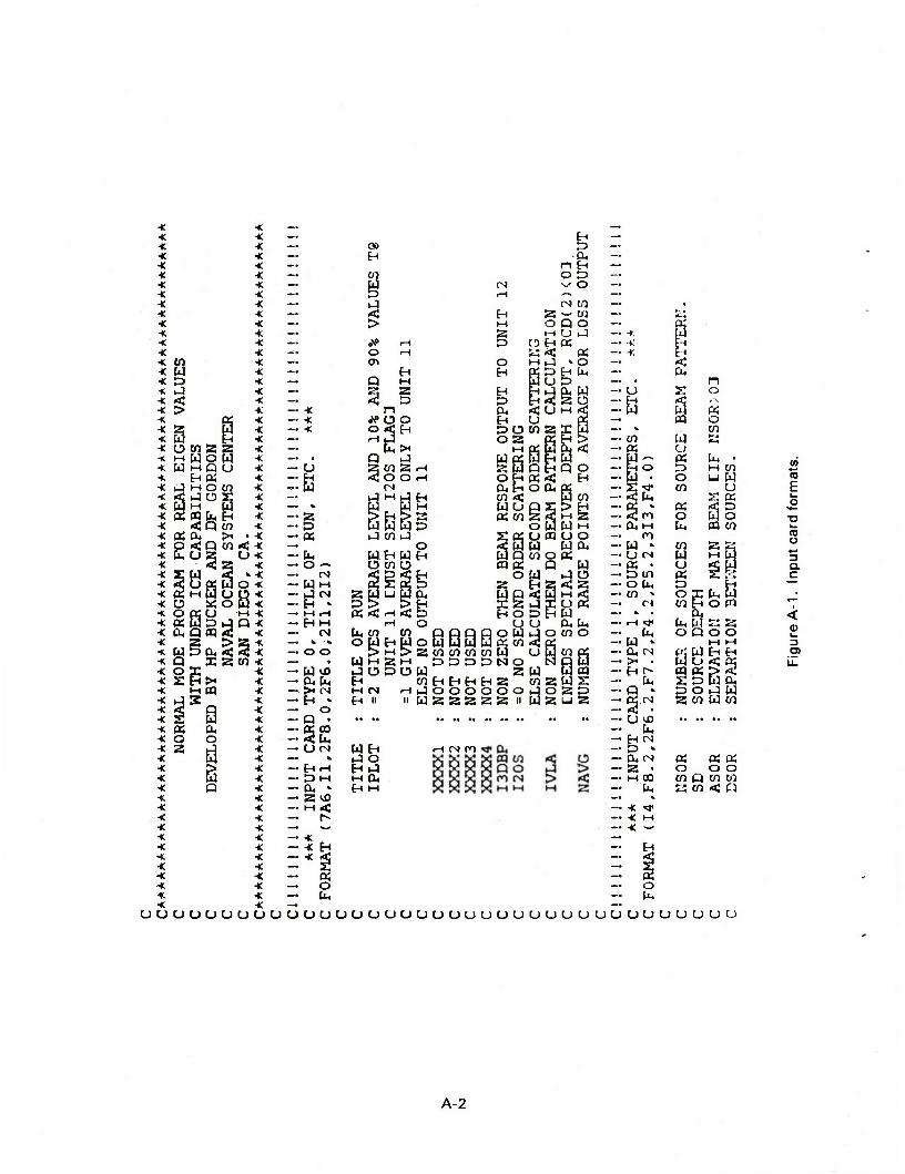
APPENDIX A: SAMPLE RUNS

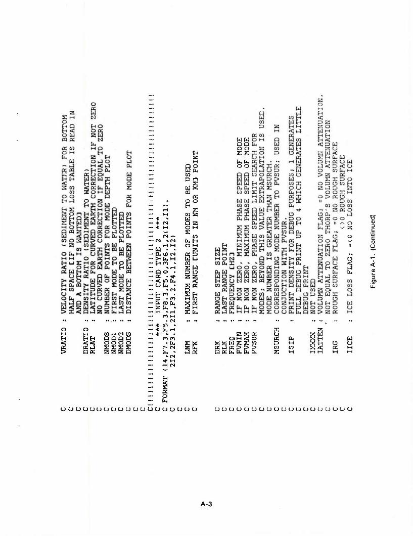
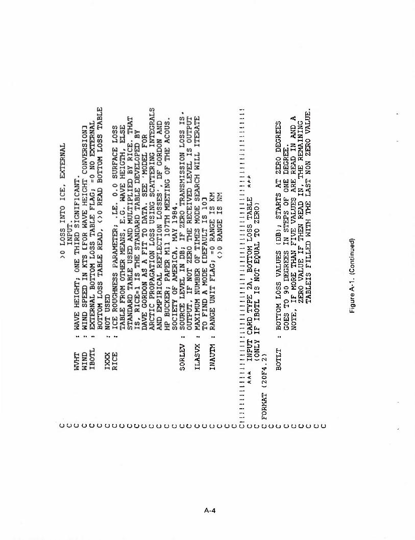
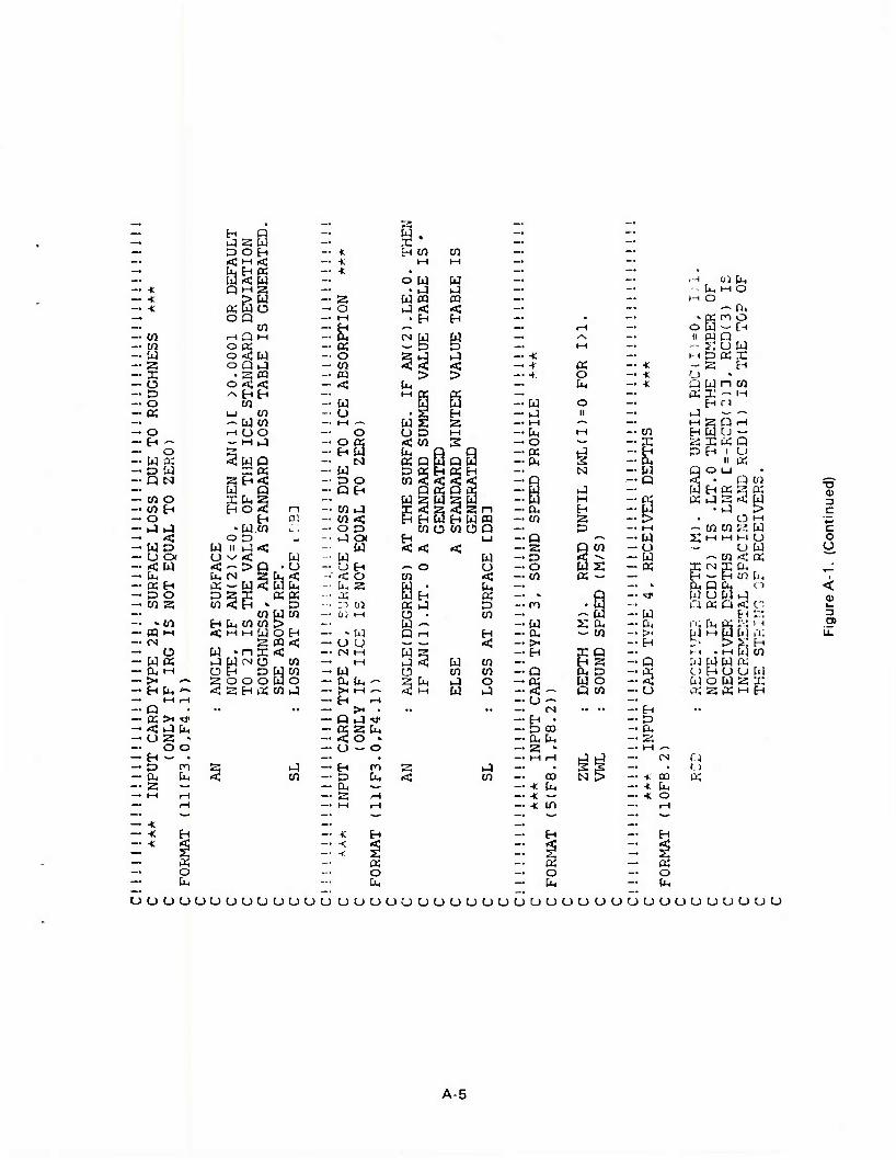
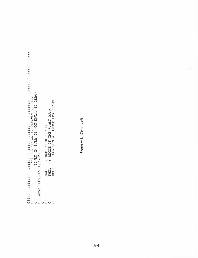
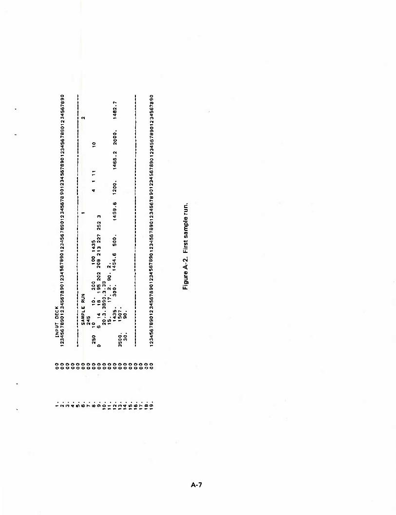
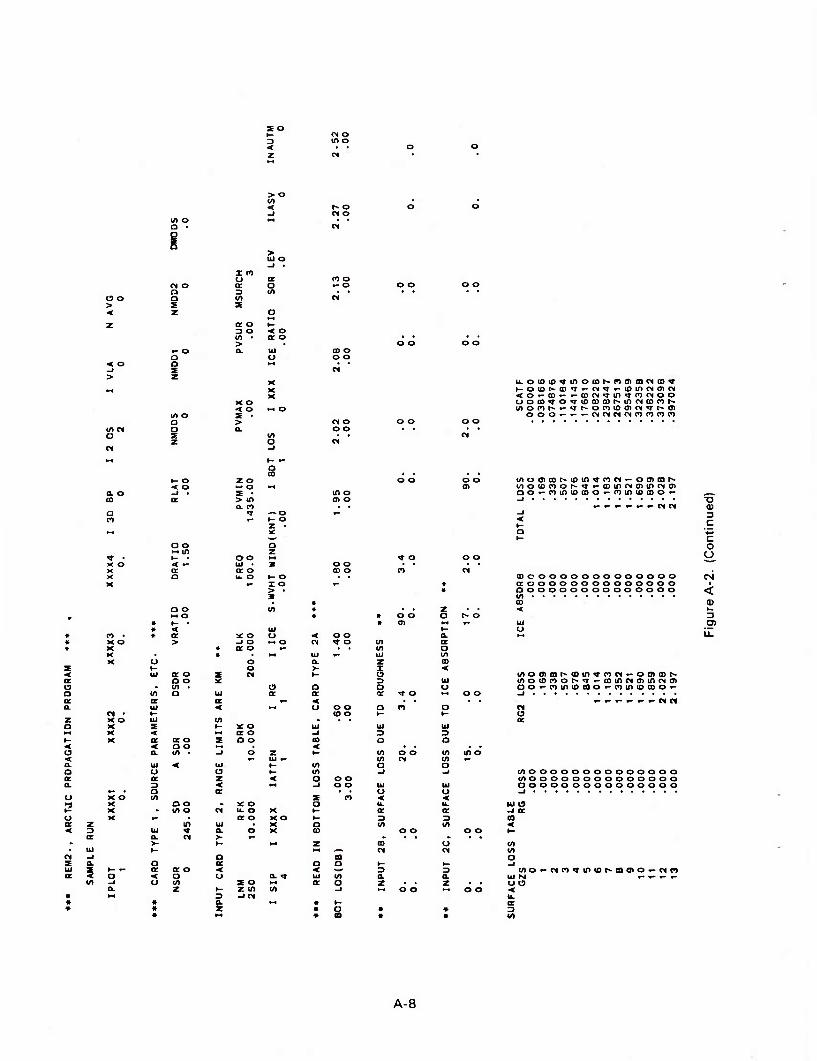
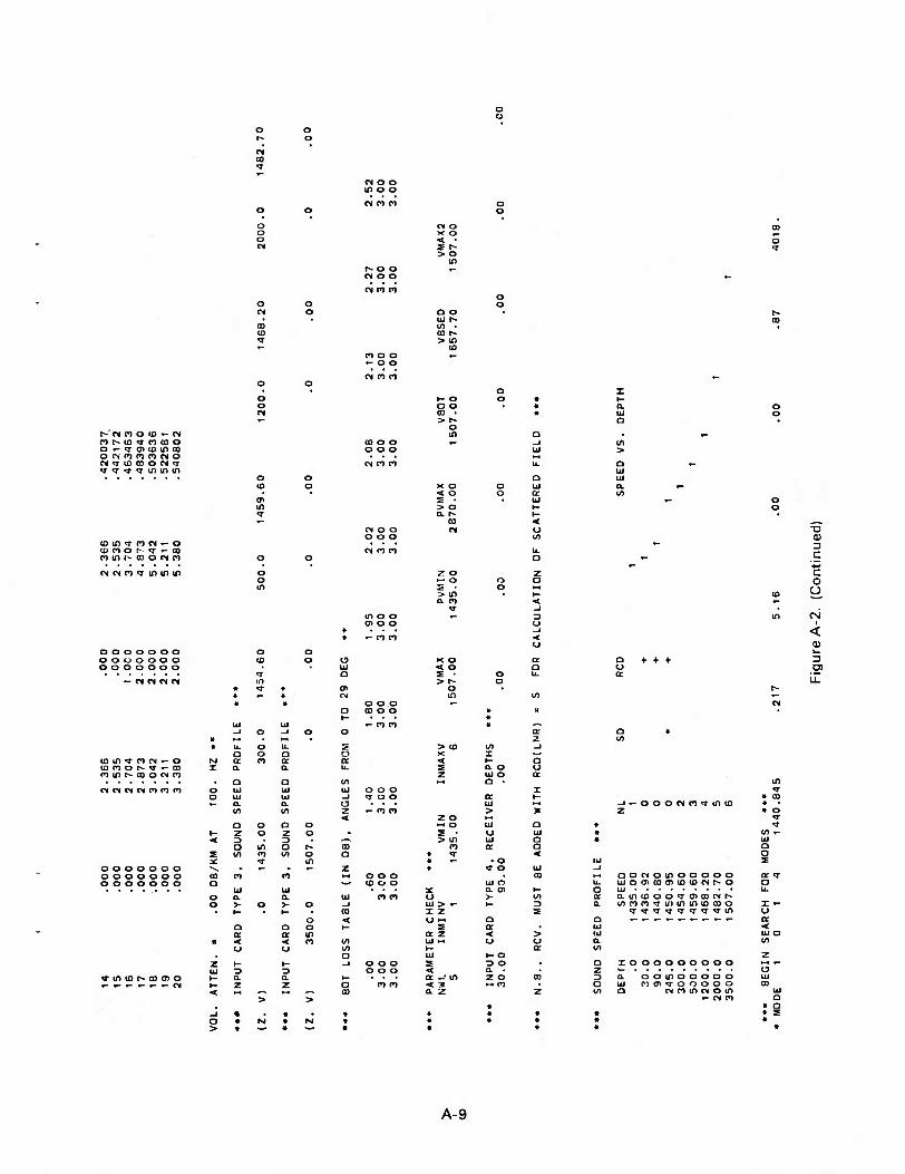
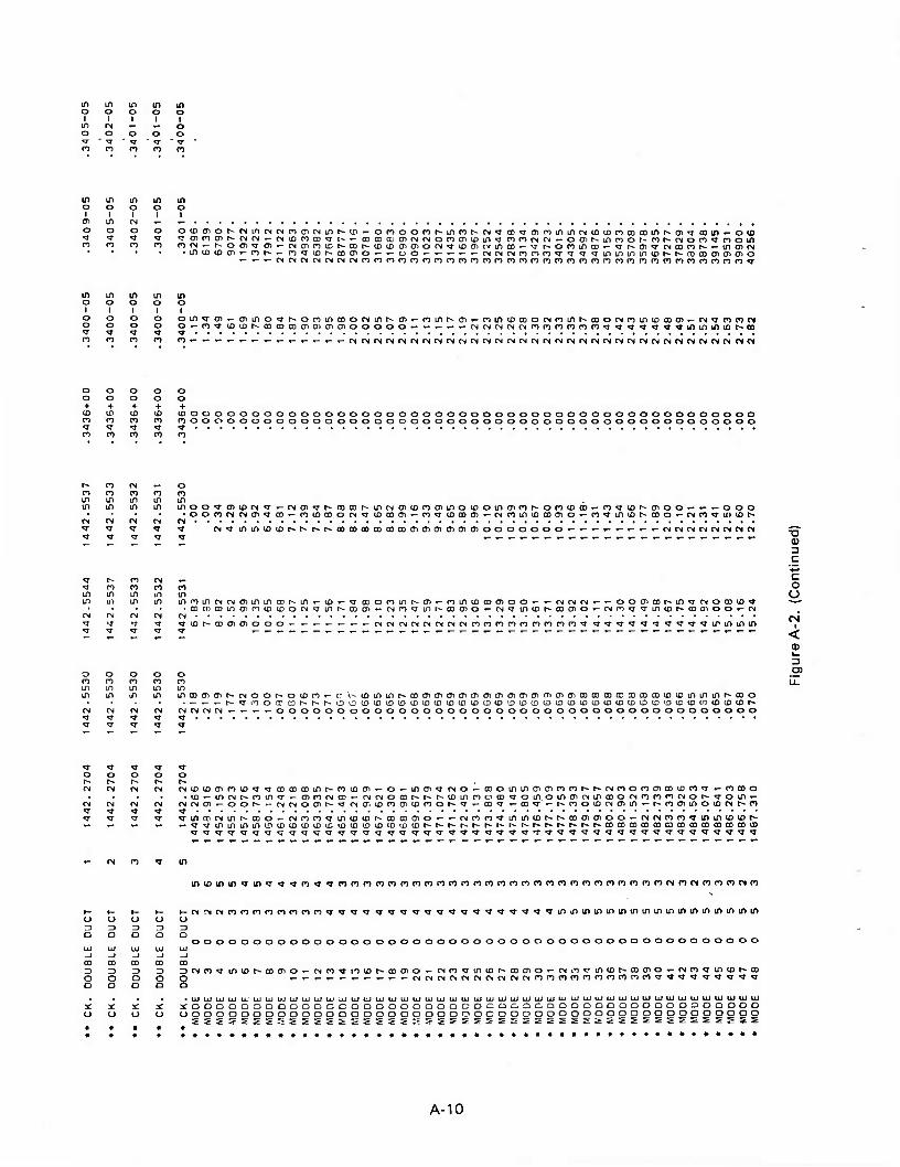
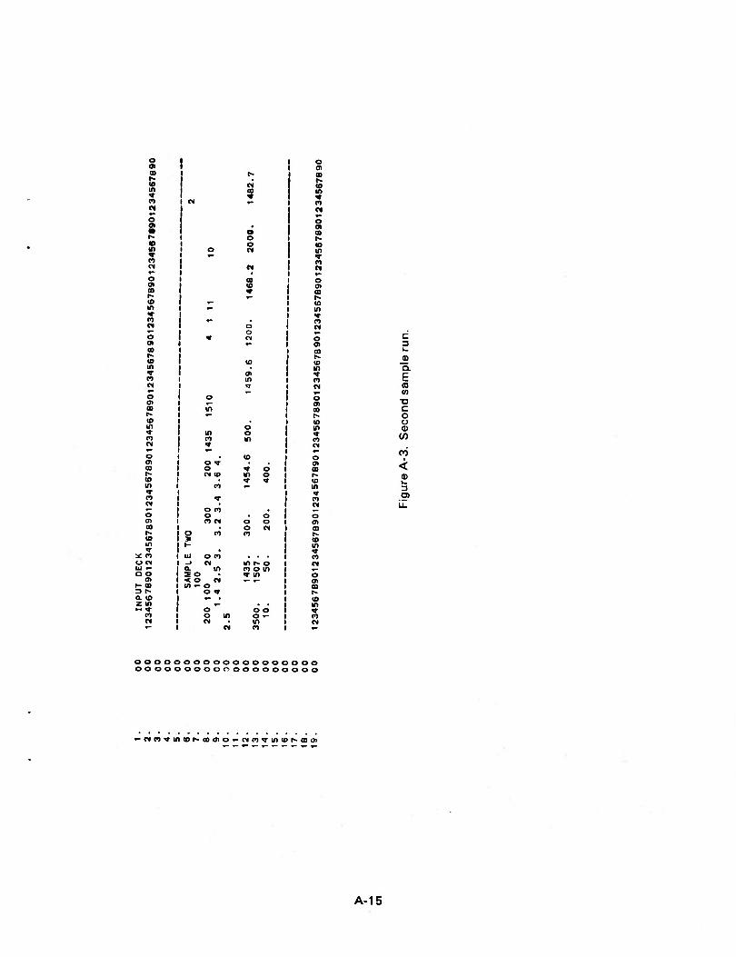
This appendix gives two sample runs to assist users of the Arctic propa- gation model in setting up run decks. Figure A-1 is an explanation of input card formats prepared by D. White of NORDA. Following that, two sample runs are presented, each of which consists of an input deck of ten cards and the computer printout which results.

The first of the two runs, entitled "First Sample Run" (fig A-2), is a 100-Hz run using 250 modes. Bottom loss, ice scattering, and ice loss tables are all read in. A five-layer Arctic sound speed profile and two receiver depths are read in. An additional receiver, at the same depth as the source, is always added by the program (if not read in by the user.)

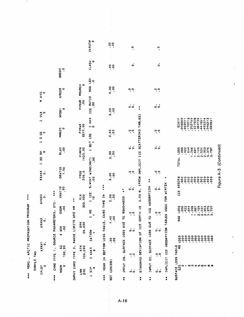
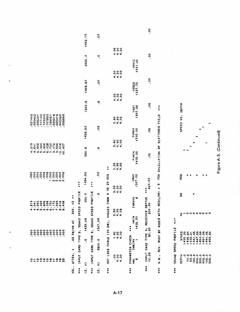
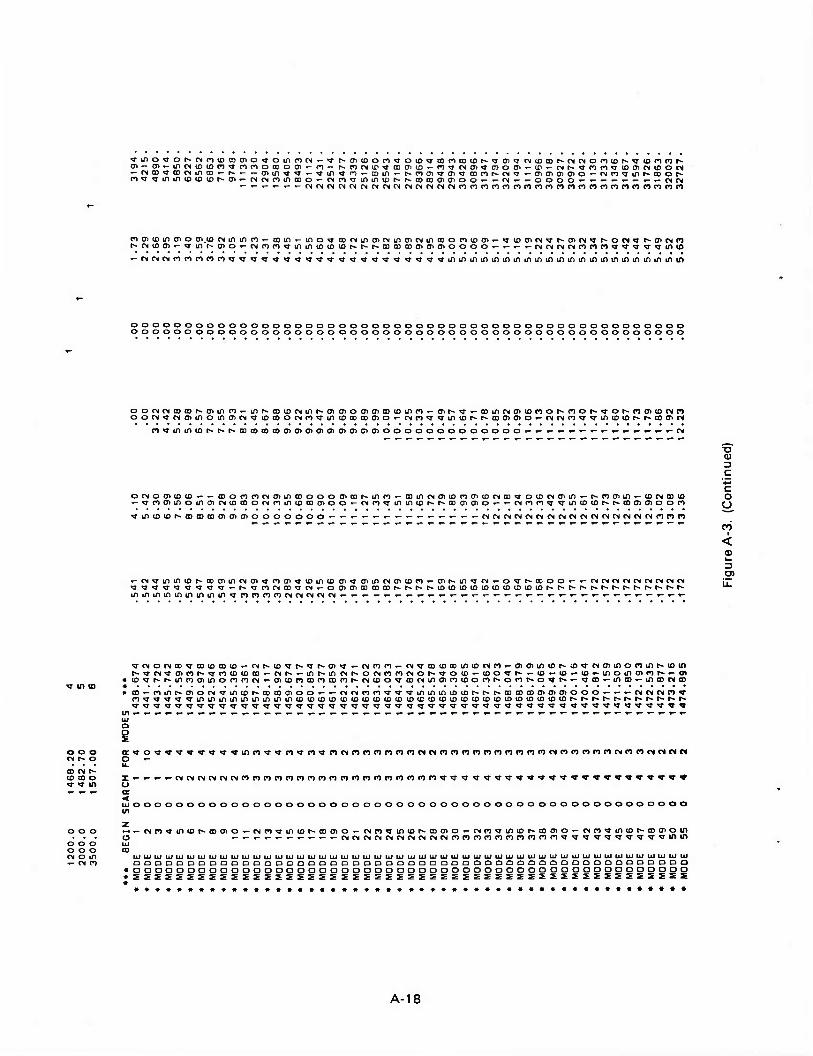
The second sample run, entitled "Second Sample Run" (fig. A-2), is a 200-Hz run and only reguests modes up to phase velocity 1510 m/sec. (This is not an adequate number, as one can check by making a run with a larger number of modes and noting the difference in propagation loss.) This run requests standard ice roughness losses for ice depth standard deviation of 2.5 m by placing only this number on the input card for ice scattering loss. The standard winter ice loss is obtained by using zero (a blank) on the ice loss card.

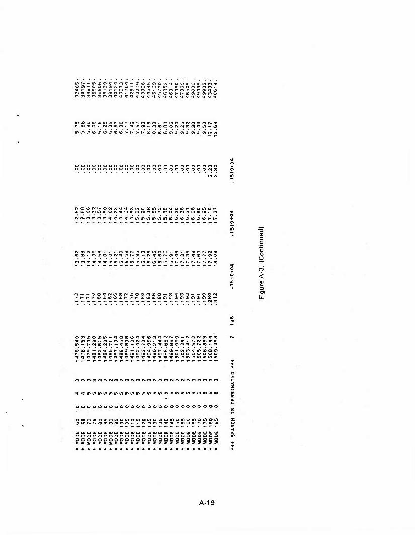
The propagation loss on the printouts is given at lines entitled RKM. The following lines, entitled 10 and 90 percent, give certain expected values resulting from the random phase relation between the coherent and incoherent fields, and are not discussed in this report. The lines entitled Coherent SL give the propagation loss of the coherent or normal mode field only. Finally, for every tenth range, a random phase loss is given, which is equivalent to the loss of a range averaged intensity.

A-1

* * ■K

*

<

* < < < *

<

< <

<

* *

< * * < <

*

* ■K < ■K

<

<

< <

<

< * < < <

-K uu

8

I a ' o to 2 M too u MQ

H« lJ M O

<

* <

<

-tc <

<

< <

*

<

a

a

H

2

«

Du o «•»

HM CN

o o

■&" o Q • a oo U CN

H-^ DM Ou «■ 2 *0 M<

o CK

oi

a

M-H f—I

h£3 wu o en J

o HWH to ü

O H 0uH to < w u « en

< -

55M

W H l-J o HP M CU

UP IS HO

wQwaM C0 CO CO W D D D N O

2 HHH2 o o o o o z a as 2 n

HNn

H: OH W U PH In j o to o u w to «

tSl P W w w « to 2 W £

O 2 p 2 LJ 2 ti

o

a,

i w u « o O CO

« o u, co w u K o o CO

o

n o

« o CO

H CO LJ U

u 5: «

öo « CO

2 2

g| O fO

2 a, y POO

a; W H H w D < a m a > < X O W Ou DOJlil 2 to U to

O o o CO P CO CO 2 to < P

<fl +-» (0 E o

x> 03 O +-* 3 a c

< L-

uuuuuuuouuuuuuuuuuuuuuuuoouuuoouuuo

A-2

es '-

w w P Q O O £ X tu U, o o

"o o IT

2 3 c o ^ o II u .v

U *- < < E 0)

<< «P P«

U1HND) PPQP o o o o XXXX a zz Q

on 2 5 «« W X X co «pa > > > P K iu Oi DH CU

x: u g to z:

to a «

w u

= I - « o

CJUCJUUUUOUUUCJUUUUUUU UUUUUUUUUUUUUUOCJUUU

A-3

a o CO

CO <

2

w m o

N CO CO o OH

sä OD H o Pw o PQH o

'S3

OS CO M

w

PQ QM

Si In U H

£s PU 2 SO ~ M ^ CS

o

o

< 5 CO CD iJ U Q2? W 2 M >

Ü MO w -ZfS« Q WM£ U

W UN o a Q « SO <J 2

U W W O NQKIiS

HWW H <2a 'to

CO Hj En U< co gor1

En CO J U co cu >«J a

w> x •'H 2 EH -!Oji)0H PQ >X S Q2HG

CO CO 2 H ij

JahStn

Q « > H CO o U CO O S O i-3 o c* « pq ►4 bU<

OHNH 3u EH

iari O O o (HU2

H >-3 H o

<L

C '■*-<

C o o

<

ai

UUUOUUUUUUUUUUUUUUUUUOUUUUUUUUUUUUUCJ

A-4

„ in Q - w . - -. — J2 U - X — — — D o H — < H to CO — - ■»• < M < - -K M M — — —• Öhß _ *

O U W — ~~

.H 0i (in — < QMS — • .-J |J — — • ■• W, H O — * > W

«UO — 2 W CQ PQ — - M O

— < — o J < <: — — — D< — OQ — l-l • EH H — • - • a m o

o 0 - [H —. CO — H — rH — — co <-i a M — a, CN U u — ^s — II w n — in o a

o5w — a — D D — M — - >: u w

- w — o 32 >-) — < — M D « X — 2 oQJ — CO •< — + « — < - 2 H — X • s m

o3< — ca > > — 4 O _ -K U

- u — < tu — U — * QWnto - D AHH — M a 1 — — « X — M — O CO — U M — W O — EH rj — « i_l CO — u • § H — i-i II — Q - -»

- U co — M -~ w 2 2 — M »-» — H 2 O -H — o ■-I u o — o U D I-H — k M — CO N0U« - H - -HJ — o a

H W < CO S — o ^^ — X 2 X« Q

— o *-* 5UP

— «aE Q W

— IX ^

— H D EH I O - W « — N — a* _ (X II « -DU x« — w D «EH

CO < < 3§ — tsi — w ÜOU

- Q N 2h< — D O — Q .— Q S • Q co ■o CD U Q - a H Q a 32 — W Q — W H « 3 a a u 2 <3 u

• j > — CO o — CO H

XtuS H o < n _ CO J

U 2[t X 3 2 EH EH W

<3n Du M EH _ Q 3

C — O H m — CO < H wm — CO 2 — £> O H V-< - .J iJ »U.co - O D co U co O Q — D — M — CO CO 2 W c - <: o D - t-J a EH u — Q >-*. — w SHHHU o -WD W ii u << - u < < < — E Q co — u U W u -UCv u ^ < w U w — D **C ^^ — u ^ CO < 0^ - < w < ~>g -u - CJ H — o u — o w s: — a INltl,

H ^ EH CO tin "

- u« UH CM 2 Clj < - ' < O CO < — CO a - — 1

— « H - UH 3 w • E — — » a, Q a. o < -DO D s £ a a — X W H Ct^ — *. Q _ <* W U W J QJ — co 3 co < H «■ D -■ t-> CO « »J D - r«"t * ^H — O a; Ci < ci u —• co W co

EH CJL, CO CO > — OJ M O • CO — 0m* W — ■u E-H 2 3

— »CO - W - — W >: cu — • D< i i- fn Ol 5:! IH [jj n U [ij »j; ?• > S H

D) — m M < M n W o EH — " M Q M H — a, ~- CO — • >« LL — CN s m < — u u < — > — •H o W -n x < — cs n W 2 _ H s§ — M • H W CO - w a JWINU co — t-H W co — — ■a fjj W W a; — CU H U EH D W CO

2 o o o W o — w CJ co en — Q a, ^> — C> H CJU til

- > -. — a. tu - 2 k, ^3 o — %r

w o — U] O U 2 X — E-i tu »- <2 H ä wq — (HH'- <; n W J — Q co — ■ o «afCHh — M r-t — EH <H — u — — - O •• — >1 . •* .. — (N •• ■• — : H •• -«><■* — Q iJ «J* _ H • — ■ D -<Jt( — a 2 CM — D oo - • IX — US » — — a. n. — • 2

o o — U ~ o _ 2 » — ■ M — - EH ~ • — > — M <-\ 1=3 d ._ CM P3 — D ro 2 i-J — H m 2 ._} — • S 2 - • • f ) — a, tu, < CO — D t, < CO — 00 M > — ■ •< CO a — 2 - — a. — — ■IC fin — • + frn — M i-l — 2 -i — -IC »- — • < O — i-H — HH M — -K in — i-H — ^» — »■» - «■» — w

_ * H

_ H _ • H — < < — —

^ : : ^ - a — a — a — • a

o — o _ o ~ o - tu - a. - u - • u OUUUUUUUUUUUUUUUUUOUUUUUUUUUUUUCJUUUUUUUUU

A-5

o -k o: * w < N in

£ O ä

3.' S f« E3 J (ffi

w 0 u3 a a 0

:: cw jj-i ^ w H re 10 u < H « ij u, 0 (OHO

zz 2: u. s > < 0} a; M OIIJ ►? H < < «C UH H

J O [lH 3 H > O UJ D M (X 2 a, t w w u *-+ UL| u3 ij a M t-l sou « D 2 H

>M CN 2 «^ i-H * ij • ■». 2in •«Oil. *_* *

r-\

• i-( »-I m .-J M X ÜH < x a, IN 2CuO

U'l

re a tu

D c c o u

< <x>

CD

uuuuuuuu

A-6

o o 01 01 CO t~ CO t- • t« 10 CM 10 in CO in •» «r v CO CM *- CO « CM «• <- o o 01 • 0) CO o eg c- o r» ID o 10 in o CM in <r r- » CO CO CM CM CM »- • «■ o CO o en lO OI co <»/ CO t- r~ c~ u> r- 10 in T- in «r * co v- • CO CM o CM »- o »- o t CM o 01 1 •- OI CO CO c~ r- 10 IO <o in ■ in «r 01 v co »- in CO CM ro I CM

o CM o 01 in OI CO CM CO t^ f~ to r- • IO in CM o in «T in CM o •T ro ro in CO CM <r CO CM

O 1 CM (0 O en i o 01 CO 1 o 00 t CO t- 1 •— o • in c~ IO 1 CM CM T 10 in i ■— in «r CM v CO 1 O O CO CM I CM 01 CM T- o m «- O 1 o in n • o 0) CM 0) CM O 01 CO r- CO o CO t~ Z CO c- 10 a • o t~ 10 in a o a> 01 — in "T »- i- CO f

* co u CO • • CO O Oi -j in i- • CM UJ •- a t ro CO o o *- O O s in T in oi o

0) < «T o in r- V- OI t- co in CM o CM w- 00 3 r- *— 10 c- a u> (0 z in • in >- «T o o o «»■

CO in O CO CO CM CM in CM *- o CO •■

c 3 i~

a. E CO (0

CM I

< a? 3

ooooooooooooooooooo ooooooooooooooooooo

»-CMco«Tin<ot»ooo)0«-CMcoviniOh.coo>

A-7

CM O in o

> o in <

i I P) O cr p> o

CM O cr o »- o o o o o a 3 m 4 4 4 4 4 4

O O o W CM > I £ < z a *-* z cr o t-

3 O < o in • er o 4 4 4 4

> • o o o o 4- o a. UJ oo o Q u o o

« o a *-• 4 •

_l I z

CM >

X u. o IDlDVinOCOt^PltSCOCMCO* ►-4 X

X »- o «C o

iDM»»4-(M»4-iomnuin T-C04-»-CDCM<rin<TC0CMOO

x o o o co^ro^TtococDt^incMcoot^ < o >-< o in o P)S4-4J[>-OP)ID01W4TMI1

in o s o o

o 004-*-4-CMCMCMCMP)P)P>P»

i/i CM i > CM O

O O o o

a in 4 4 CM z a CM

CM -j

t-i 1- m a CD

1- o Z O o o O O in o o>cot~ioin4»p)cM»-oo)coi~ •c o *—. o 4-4 0> in o iDPioi^^r»-cDincMO)incMCJi

a. o m

) 4

> to in o O) O

o o 4-niniocoo4-ninioci)0 4- T3 cr

cr p> • 4 a) Q 1 — o T- _i 3 P) •* (- o

Z • < 1- C

1-4

O O 4-t in

Q z

o l- c

o o <J" • t- • oo 4-4 V o o o

X o < f UJ • X o o 4 4 4 4

X cr cr o CO o n CM X a u- o 1- o 4 • m o ooooooooooooo oi X *~ I o > •

X

•" • * cr o o o

ooooooooooooo ooooooooooooo

1

< • m 0J

O o ui « • • z 4 • < h- » • 1- • < UJ

# * *

o o en

o 4-4

t~ o HI u

3

» p> • • a ■x. o u < o o Q. 4-4 U- * x o > -i o i-i o CM <* o in cr • X

X X i_>

* * cr o

o 1—1 UJ

a. ~ m UJ z

O in m

\ >- o >- X < Ul a o JE CM I- o inoo>cot-.iDin>tP)cM»-oO)CDt»

a o o S i UJ in o iop)oi~T4-ooincMcJiincMci>

o cr

to IX

in • a UJ

cr

o cr

ft» Q cr < * o

u o o

O o 4-p)iniocoo4-P)miDa)o«-

Q- CM •

tu *- < m o o o (0 o

o 4-

PI o i-

CM <3

z X o UJ in - 4 • ■ a X ■ t- * o in III Ul 4-4 X < *-« cr o -i 3 3 t- X or a. o s a o m a O •< < o o • < 4 4 • • a OL in • _i o z H- in o o in in o * *- UJ T- m CM in »a a- 111 < UJ >- in o a o o (3 1- m -j -* tnoooooooooooooo cr cr z < o o o tnoooooooooooooo a. 3

o t/i

< at

4-4 _i o o III o <

UJ ooooooooooooooo

u X o z p>

3 X a o • x o o u. ti- UJ o X » in o CM ti- o X >- cr er -1 ex

o X *- • er o xo t- 3 u 03 <r z in UJ • X o in in < < =3 III V a o X m o o o o 1-

<r a CM >- 4— - • • •> • • * > i- 4-4 z ■ o M • UJ t- 4-4 ^— CM CM in oj _i a CO o I a. o ac a 5 t- >— -i Hi z 1- »- ■ er o < < <—' 3 -D in o »-CMP>Win<Df-C0CflO — CMP» a < o < O o a. v UJ in a. a. U IM ft" »ft •■ ftp»

in -1 u m z o cr o z > z • • u o a z >- z m in _i 4-4 o o o o < • 4-4 3 -J CM u. » • I M • t- cr # » » 8 • » 3 • •-• * * • in

A-8

o o

CM CO

IN O O moo

o o

o o

i» o o noo

o o

00 ID

o o UJ r- co • m r~ > in

(0 noo «— <- o o

r- CN en o co «- c* ro h* 10 «r en co o O *- «T (J> (O if) CO ownnoMO CN rr co co o IN <r *r *r T *t in in in

co co o r-« «T «- co p) in t- co o CN n

c* CN cn ^r in in in

o o o o o o o o o o o o o o o o o o o o o

— CN CN CN a

• o o h- O o o a o PI CO • ft" > f-

o in

CO o o r~

o o o

rM co ro

o o 03 o X o o • < O o 01 s • ■

in > o f a r- «-

o

CM

o o o o

ro ro

CO

o o

o z o o i— o o in

* in 01

o o o o

ro ro

IE > a

in ro

o

o o u> o to

UJ x o < o

T a 5 • o in > 1» o T * 01 o »- * EN in * o o .o •—

O CO o o ft

o -I UJ

o

z o

<

DC o

I h- Q. Ul o

>

o o

Q

-a 0)

c c o u CN

I

< 01 I—

D

CM

5 a

Q Ul

to in t n ci t- o rsl cr ro cr cr < i- a co ro o r~ *f •■ oo I a. a. u- £ Q- o o ro in r- oo o cn ro

o Q Ul Z LU

a o cr

in CM CM CM CM co co co o HI UJ UJ o o o X >r

o LU UJ _1 <* o o cr h- ft 00 v- a a o • • UJ —4 _i v- O o o n co <r in to • •

LO Ul z *— ro ro > 31 z ft o < z o *-« »r Q o o o t-t o UJ a * <»

1- Z o z o > 5 u UJ * U1 r- < 3 O in O r- ■ > in

ro UJ cr

a a

« UJ a

s Ul ro in o a ft T < o K v in ft r~ * o IU £

o o o o o o o >v - »— - *- z ft <T o UJ _l o o o o o o o m CO ro ►H o o o t CO *-* Q O Oi o in o o o o o cr q- o o o o o o o Q

UJ UJ ** to o o * UJ

a o OI ►- a

UJ UJ

o OI CO 01 to tO CM l> o O U-

o a a. UJ ro ro o > t/i a: a in 10 o o T 01 CO CM r- o >- o > o _> UJ > r- H => CL Ul ro m <r i/i in in to co o I f

h- i- CO I z £ »T ^ I i ^ 1 1 <T in o o < u M Q Q cr

Q a o H E cr UJ < cr or in cr Z <t > IU Ul o

(1 < CO w to o

UJ

UJ i- o

o cr

a 10

Iff

z z i- >- _J o o o 5 ID o • a I O o o o o O o O o ft r-

UJ 3 O o o o < O- z •— o v in co «» oo oi o y- a Q. t- cr • tn z o ■ r> Q. o o in o O O O o UJ

t- z Z a ro ro < 3: t—1 ro o UJ 01 Oil o O O O o CO < > > m a. Z

ft z in a CM CO in CM o

»- CM in ro

UJ a

» o _i • . ■ • * • ft » * • s o » M * N * » ft * « * > » * • ft

A-9

I LI

in O

I

I

oißoior^csMnrgcNroaicNinr^u}^onoonr-innr~cN^co*TC7>c'iinino4iDiDr>CD(X>inr~a>*TCOin»-ou} lOinmsnrt'-nionro'jt-'-iijroaiOipinooonDin'jnnnpi'-ooihinriot-nNnoninoui

• tn(D<DD>i"nN^,n^iDNOOio«'«*oo«>*>'^,<-nNoinnnv9|v^u)ifttfiinÖNb'ncDotoioio '-t-'-ncNoitNPJOKNntnnnnnnnnnnnnDnnnnnnnnnnonnnnnnn'j

in in in o o o

o o o (-> o o <J <r «J n tn n

oln^I01'-(Tllno'J^o^ln[t)otNln^Ol»-(nln^Ol^nln^ocooMnln^cDo(Nnln^ocool^^^'JnnM o^(0^uDU)t^a3cDcoaio>oic7iooooo^^^^^r^r^MCNCNcntr)r)tTir)cTi<j<TTi^T^T<r«Tininintoh-eo «T

+ ID lOOOOOOOOOOOOOOOOOOOOOOOOOOOOOOOOOOOOOOOOOOOOOOOO

nooooooooooooooooooooooooooooooooooooooooooooooo «3 en

IN ra rj CN IN <r >» <? ■7 t «» t ^ <T t

m in inoovoi(Doi"j^C((n<TMO(DMnMOiii)noiinoiooinfnnNoniflCD'-n'HDMjioo^f^ooo

oonrjwoi^O'-niD03orN^a)aD^^nviiocDoi'-(Nnif)iDa30)OT.n'Tir)u>h-a>oi-Mn'TU)«iih

T3 CD

C

D in i/i<v)^tNCNmLnincDMn^(0»-'Jcooni^NOi--nif)iX)CD(DOO'-'-fNC\rj 'CD(TicoixiairoiDU3otN'jinr*cDcri'-c\n«jinNCDOiO'-(N<5i/iiDr*aooio

"JlDMDOIClOOO cNr<r<tNrtMCNr<nnnnnronnn'j«t*T,T<JT^<J<jNT<firir)inin

C o U

<

inmaiOir^cNoor^oiDn^cWiDininr^roo^cDaiCDCTicTit^

OJ OJ OJ CN -- •- *- .- oooooooooooooooooooooooooooooooooooooooo

ID to oi n iß vT c cDcDcDi/iNntoai'-O'-i/itJi^'CNO'-CDOinifiCTioinnNh'Ojnorooffliowt •- D co o ^J^ln^^^ln^^ffln^^cc»-cN^^ocD^^^^Oln^oa)^o^noln(ylI>llncoo^(n^^OlO^'IOln•- oj a> *~ o o t-~ --c^cNoair-^TCNff. iorr)(7iioroot*-Tj-»~a><3' *-aD«T"«-o-mo(Doia>in*-o-c»j-oiinoiooif-f*) in m fN m o* m O J OJ m m ^r m en ui r- IT m m o vm ^ CN n r> <3" U"l in (D r- r^ CD cn CD o o _ OJ OJ n O <7 m m CD to r- <T T in in in in 10 10 (O <.o in m (0 in in tn m *o tn r* r» r- t^ r- r- r- t- r- h» t- r- h- r» r- cu CD CD ÜJ ÜJ CJ cu QJ cu m a) CÜ OJ <r *r <T rr ^ <T <T ^r <? T c <3" <7 T <T <T <T ^7 tj <r •? <r *3" ^T «3" ■3" ^T T T ■NT <T *3" ■<? <T ■3- •3 <3- ■<T •3" *T <? <T *3- <T «T <3 <T

►_ |_ i_ (- i-rv^«nnnnnnnn^sr^NT^^7v^g^c7VvT^^vTvTinLOini:iiniriini^i/iinüiinin^inmm o u u u u 3 3 3 3 3 O O Q O O

OOOOOOOOOOOOODOOOOOOOOOOOOOOOOOOOOOOOOOOOOOOOOO uj ui uj ui UJ I I i I —I CD CD CD CD CO 3 3 3 3 30jn^in(or^cDci)OT-«n^nu>^a)cno^csn^iniONa)cno^w^viniD^a3(Jio^rtn^i^tONa)

O O O O O

. uJ iij LJJ UJ U. UJ UJ UJ UJ UJ UJ UJ UJ UJ LU t-U' UJ LU UJ UJ LU UJ UJ UJ LU UJ lij UJ Uj U U UJ LÜ lL' UI lULÜLÜLJUJUJUlULJlUUUJ a: Y. X :£ ^DQDOO^QOOOCCCOQQOOOOOOOOCOOOCiQQQDQOClDQODQOQOCJOO (J U> O U UOOOOOOOODOOOOOOOOOOOOCOOCOOOOOOOOOOOOOOOOOOaQOO

A-10

crrir^^ncNrocor^cDronoai^m^oocnujooiniricTir-crrjooro^TtNt^r--*- tn(Ti^cD^ro<T^^«rLr>^rocr>cNr*^TcN'--o--r)ir)r^orr)t^»-ii)--<i)'i~tN'3-tDo>rQ ooojnintDh-mainxLnnoCTih-iDin^ntN^OCTicncot^f-ujtr'inin^TocN'-T-

^OOinCV0)CD(T)CDr-^ICJiN'-o^"(0aD[t)CDCDlDC0C0(D0D0Da)njCDCDtD0DCDCDC0a)

cNnnrn^^^^^iot^r-t^r^^cocDrocDCDcocDCDcocoaacDCDtDCDODcococDCDcocD

OOOOOOOOO^CN»-CTilOtDOOr-CNin(DtDmrnOh-fT)CD'TCTl<TCD!^t^t^CO'- ooooooooocN'-iniot-t^r-cD*TrO'-o>t~-inn-~a)a)r)»-a3iDna)roa)(Y)0>

cN<rin<or»-coa)0 rNCOO^jmiot^r- cDcnooT-wnmiDiDOi --«-CNCNOICNtNCNOJCNP*

oiQotNnrtoi<rr-a)fnocj>»-inor^if)^TTinr>-o^rcy>«Toco^rrNOCT>oi'-^''-«~cn

CNc\nn^^c'u^ir>ipu)ot^h-h-cooooia)00'---c>ir)fr)'T^Tininti>t^coa)OMcn

c^oiu3^^inio^c^r^>T(j)tDi/iiDcO'--(£>cNa>r-i£)iniDCDoror--ojts-rr)OLn<Tinois- romt^^^r^of^u)aicNinCT>irir-»-u?oin(T>'TOi^ia)<Toir)oci)--r^ro^Tti)QD»-n

cNr>*-r-rTiaincN^otNnfNCNiDt-r-ricDr*iaonai^roiO"-r~-'Tor-rrflD'r'-oo r-r^tccD0^CT)OooijicDor^»3-oc)'-fT)«Tü)i^aiocN'?ir)r-cpoc^fr)ir)CDCN(Do^' oooooo<-'~^»--^o«c^o*cNCNro(T)mr>(Tirotr^r«3-^r^T'q-inininininu3tßr--r*

0) 3 c c o a

CM ■ <

CD k- 3

cD»-*-Of-n»-^wnoinncncoi/i'-NNrtT-«oi(NN(Dn«-<ionn(NP)oo« inoiD<rinooinr-rN'-cn<rrir^inr»-cNfNr-r-rN^rnCTt^Tai^'OCTi'-a>«-o^ooo> a)^oto^cDontD--a>oiriait--cD--t^ininco'Tc(fniDr)rNin--CT>cNr>.or-^'<j>^

r- 03 ,_ n Ifi m ,_ n in m o o t-- o <r m n r» CN r* <N CO *r o ID m o r- in CN ^ CD oo r- CD CN ao CT) m CD 0) Cl) 0) a o o o *- »- ,— og fN rw r> n <J tj m m in r» r- m 0) en o *- CN CN <? U) CO ■- n ^T v <J <T ■^ <r if) in in in in m m in in m m in in in in m in m in m in m UJ UJ ID UJ UJ m UJ t-~ r-

ooooooooooooooooooooooooooooooooooooo

c omo'Xioinoinoinoinoinoinoinoinotnoinoinoinoinoooooo ^inmi£>uDr-r-a)CDCT)CT>oo'- «-n(Nnn<i <r:niniDior--t-CDCDcncno»-CNn^in

UiUJIJuJUJlJUJllJtiJUJUJlJliJUJUJUJUJuJUJUJUJLJUJUJliJUJUiUJUJliJUJUJUJuJUJlJUl aOOOOODODDQOOQOODaDOnoOODQDQOOCiOClODOQ ooooooooooooooooooooocooooooooooooooo

A-11

-a

c c o o

_1 in

CM I

< CD k* 3 TO

CM »- •- CO o *-

o> o T en O* *D Oi c> r- ,- O CO r- r- r- ID r- r- CD r- r^ CD CP r-

Ol Ol 1 n ■- o co t- co CD en co

o — in m 01 ID T Ol CD CO 00 01 CO Ol

I/) »- CO CO t- r- to CO I-

CM •- — I» co CO d t**

in CO

in •- en co

ID 01

n co

Ol

in co

co co

Ol CO

o Ol

O CO O CO

Ol Ol

01 O V CO in oi en co o I- Oi 10 t- f «J- co in o •■ ro in CO t» - CM «- in CM V Ol

CO ID

V CD r- co

Ol ID c~

CO «T co r»

— Ol CO t-

CD CM CO

Oi CO oi h-

CO en

en r-

in CD

co r- CD in m

in — oi to Ol

1» CD

co «r 01 CD en

ID CO Ol 00

CO CO

> Ld o o o o o o o o o o <J o o o o o o o o o cr Z

1 o

_l o o o

_J o

_l o

_J o

_l o

_l o

_j - cr o t~ 1- in o o o ►- ►- in o l- l- in o 1- 1- L0 o t- t- in o H- f- in o t- *- LO -i w- z z r- ■- Oi z z m z z T z z in z Z ID z z t- z z UJ UJ UJ i- UJ UJ i- LU UJ h- UJ UJ 1- UJ UJ t- LU LU t- UJ LU *- > u o z o o z o u z o o z o o z O <J z o u z LU 1 1 UJ 1 1 UJ 1 1 UJ 1 1 UJ 1 1 LU 1 1 Ul 1 1 LU _J or or cc at or or cr or or or cr or cr or cr or or cc or or or

UJ UJ LU UJ UJ UJ UJ UJ UJ UJ UJ UJ LU UJ UJ UJ LU LU LU UJ UJ o a a. X rs a a. X a. a I a. a. I o. a X a a. I a a X z E O o S S O s O s O T£ o 5 o SE o 3 * o o o o 5C X o o CJ X o o o 3C o o o * o o o * o o o 3C o o <J o cc — Ol z cr or — Ol or — Ol CC ■r- Ol cr «- 01 cc *- Ol or «• o> LO «c

A-12

01 (Du) — 00 01 CD 01

o

cn 0) t- 01 CO oi

f o O Ol

00

o »■ 01 O CO

CD <T in ID <r co Ol r- >J 1 O Ol o Ol O Ol 01 Ol O Ol

O *- "-CD in

oi o r- O CO

in oi

CN CD O CD

in oi

ex in cn oi

in CM o cn

co «r o cn

oi Ol

oi in o oi

m o

o o

O L0 ■r- cn

T3 CD

C

CD »- n f- t» •- cn

c o

CN i

< k.

in T Ol CN CO Ol O CO «r o Ol CD CO Ol O CD O Ol O Ol

co in cn cn

CD CN O 01

r~ co O 01

t~ co O Ol

Ol Ol

oi in o cn

o «- i- o •- oi

o o o o o o o o o o o o o o o o o o o o o

-1 o

_j o

-1 o o o _» o

-J o

_J o

_J o

o 1- l- in o h- t- co o i- ►- in o o o v- t- in o *- ♦- in o y- *- in o f- i- in o ►- i- m z z Ol z z o z z o o ~- z z CN z z ro z z *T z z in z z

1Ü UJ f- UJ UJ l- ■— UJ UJ *- *— »— V- UJ ui t- — UJ UJ t— »— UJ UJ t- »— UJ UJ t- r- UJ UJ 0 o

1 1 z UJ 1 1

z UJ 1 1

z UJ 1 1

z UJ 1 1

z UJ 1 1

z UJ 1 1

z UJ

u o 1 1

er er er a er er er er er a er er er er er er er er er er er er er UJ UJ UJ UJ UJ UJ UJ UJ UJ UJ UJ UJ UJ UJ UJ UJ UJ UJ UJ UJ UJ UJ UI a a. I a a. X a a I 5 o. a X ex a. I a a. I a a I a a.

s O £ o s o o S £ o E O S D s O S ■x. o o o :r o o u :r o o CJ Q * ic o o o -c: o o u *. o o ej 2C o o O * o o er — Ol er •- cn er r- Ol Z er er — cn er «- 01 er — 01 er — Ol er .- 01

A-13

oia}oic*)«-r'~^(0«-aia)tnaioi<roair>»'-df- o«*>

oioor-ujor-iocNcNoioii-oioaiTinujcNro Din 0> O •- Ol O Ol O Ol O O «-0 O O «- Ol o o <- o »- o o

mna>orit~o«*«rr-»-c<iu>f-oo*oa)Mn>cn *-a)

t*-atr-ionooi*'«mvooi<?in«-minioc*« ^- in ooiooioo<-cnoo*-o*-o«-o*-o«-0'- oo

tu a

in co —n at ci to oo u> o n T c< to oao CN IN into in o no • • s 01 >■ no a) n not n in Ar ai in mn s 10 ion n U)io OO'-01OO*-01«-O'-Or-O<-O*-O*-O«- OO~J

cc r- Z o u

o o o o o o o O O O o o ooz o o o o o oo«

_l. _l. _J. _l. _l. _!•• mOr-»-l/10»-»-l/)Or-r-l/>0»-*-l/IO»~»-(n OOI

ID Z Z IV Z Z CDZZ OIZZ OZZ OO *- t- UJUJ I- *• UJ LÜ t— «- U U t— «- lü Id h- CN 111 111 I- Cl 04 O Z UUZ OOZ UUZ UUZ UOZ UJ UJ I I UJ I I UJ I I UJ I I UJ I I UJ IT a. Qrorcr cc EX cc a a a cc cc cc or a: or o UJ UJ UJ UJ UJ UJ UJ UJ UJ UJ UJ LU UJ UJ UJ UJ Z T aax O.Q.X O.O.X a n. i a a. i s o OS OS OS OS OS o o s ►* UXOOUXOOUXOOUSCOOUXOOCJ 03C

cc »- en a — en a — oi or .- ai ir<-o> z or < < r- ae <

Q

S

C o o

I

<

3

A-14

o 01 ■ r» r- 10 CM m ? n CM *• ft *• o a> • m o t- o 10 o » o CM * *- n CM CM t- o CO 0> j 10 OS 1 * c» 10 1 r-

in i r~

* i <•» i ,_ . CM i o «- I o o 1 » c\ an I as I t- I 10 1 10 in i «■ 1 en CO 1 in CM 1 «3 •■ 1 O 1 o Ol 1 a) 1 in r- I 10 I , in 1 o * 1 in o co i ro in Cl i «r *~ I •— O 1 • (0 en 1 O «T 00 1 o • o t~ 1 CM 10 in o (0 1 ■ «r <r in i ro •* I (>J I V CM i •■ I O 1»» • O 1 o • o o> 1 ro CM o o ID 1 o CM •* I o ro ro 10 1 3 m | 1- <r 1 »

x co i UJ o m • > O CM 1 _l CM in r» o UJ - I a. in noin a o i 5 o ■T in

O) I < o CM *~ r- t- a i in — o 3 t- 1 O V a to I z in | f* • . •-■ »r 1 o o o

co I o in o V-

CM I CM in »- i CM CO

o ai a>

CO CM »» O 01 oo r- O) in

CO CM

01 CO f- 10 in <r CO CM

O 01

to in

ro CM

o Ol CO f- to in «r ro CM

o 01 CO r~ IO in T ro CM

ID in «r ro CM

O Ol CO r- ID in

ro CM

ooooooooooooooooooo ooooooooooooooooooo

»-cMro»in«oc»cocno^-CMco>JiniDr-cocn

A-15

in o o • o S 5

o o o o

> UJ o _i •

I PI <J or o o

CM O cr O o o a D in

13 O o W >r > E E < z o Z IT O

3 O V) • >

< a:

o o

T- o a. UJ o o Q u ID O < o o 1-4

-1 E P) > Z X *-«

in a

o X O < o E • > o

X X

o o o

in CM o a. *- ■» o O E in in

CD <

z

Ü. o t-n en om »-^ n ♦• t-Ot^r-CT-fDCOOlf-t^t*) <oi/i»nNO)tNiDfOwa) UON(Drt--'Jr-P)OlM i/)oo>NintM»tioi'j CD

oo^-cNnoTTinin

o m

1- o z o < o t-< o n a. o -} • S • o o o or > in

a m CM O

Q v ~o PI p> <■ 1- o

z • »-« X.

o o a *-« in z » • »- o o »-• X o < T- UJ • a O O X tr or o o o x Q u. o >- o • • X Pi I o > • PI

inon^iDNa--niftt* in o CM t n» co o ri in t~ o> ootcDojiO'-iniJiPit-

C t- ■- CM CM Ol PI PI

-J < t- O t-

■3 C o

00

< moooooooooo CD oroooooooooo ooooooooooo 3

m

PI • X o

o o or

z D

CL o

DZ O □ O

O

Or

O O in o

o o •9 O

in

CM

a. <x D

a: o

I 13

o

X a tr o < a o a in •

UJ < u a: z>

v • o X o in X a o X - m o X «— •

o o 3 UJ o f- Q. »- > UJ l- _J a Q E t- o a at o < o «t o in —J u in

a z

i- xo ►H or o X o o -I o

CM UJ 13 z

X o CM U. O

a o

_-l 3 m o •< t-

in w o in _i

n o o _j o O UJ

u

o rs *■" o o

in o UJ f- -J

o UJ < 3 t- n • • z m o o o

wocMviot^cn^-Piinr- mooj<TiDa>oP)int~o» oo^mpiiDr-inoint*

•- .- CM CM CM P> PI

O O

O Or < u

E O I- z o 3 -I CM

X X o X X

CO a a «r ■—

o m

o CM

z • - •-• P> o

z □

> UJ O

Q CC < Q Z < i— m

m o

cc

in

D in

CM O

inoooooooooo tnoooooooooo ooooooooooo

<-i o o •-■

ui a -i a

ino»-cMPi»»in<oc-coci> UJ tsl u o

in

A-16

o o

CO

o o o

o o

o o o o o o

> o

CO h- > in

o o

o o o o o o

o o CM

o o

0)n<-icoor-tDoo0) «TCT)0"»*Tr*)cnin--r~coo> igrt^noiflpicnoifl *-tDcor~ror-cocoiniNio lfl(DU)NNNr*CD!BCOa)

■•-<TU3coocMinr~cF)T-co ouiovffimN'-inov *r«ytnininiJ3r-a>aioo

o o o to o o

01 in T

o o o «too

X o < o s • > o a. r-

it)

z o n O E ■ > in a. n

CO >

Q. l/>

■o 0) D C •*- c o u CO

I

<

CD ooooooooooo ooooooooooo ooooooooooo

o in

1 in

UJ K O < o

CJ g • o > r- o

01 o CM in o

o o o »- o U o o o * V

a u

(x-ntroigontioo *-<yißcooojinr~ö>'-ro cMiDo<TO>cor~*-ino«»

«r'Tinminioiot^ocoa)

ooooooooooo ooooooooooo ooooooooooo

o o

o — MHVMSMSO

N a: ro cr cr < ►- □ X a.

a

a.

Q

u.

m Z

a. UJ Q

o o

u cr

o UJ UJ UJ o o o o I o UJ UJ -i moo cr o i- CM a. a. o • • • UJ CM t-4

in in z CX T «T > ■ < z o *-* o o a o t—* o UJ Q •

»- z o z o K 5 • o UJ • < 3 3 . . > in UJ Q *

O in o r» m n cr a z in n in o a » >» < it «r in « r- - o UJ \ • «- - *— z * T o UJ -1

CD p) in ►-< o o o • CO — O ■—i «TOO UJ o u.

IU UJ • • • X a. in 1- o o a. a. UJ - «r v o >- m cr o V o >- o _J UJ > *- l- Z3 a

h- t- o I z i o 1 <-> •-< o a

o Q o t- I cr UJ cr cr in tc < > UJ

M < < en in in O

UJ ►- UJ

" h- o

cr a. in

Z ►- f- _j o o o s => O • Q IU 3 3 o o o < a z 1- a a. i- • cr _» in Z O CO D 1- z z o 1 <T < * *-* •— O < ** i— ■ a. z z in

a in

-J — OOOOCMOOI z

oo<r«-incooi7iino utou)n«o)<Dot<o UJ a. in in m ._ r- <T t- ,_ 01 tn n n n f <T in m t m

<T <T T T <? <T «» «T V

XOOOOOOOOO *- a. oooooooo UJ T-LDOOOOOO

o *- ex n v *- m

A-17

u»-o>'-infMU)ion9n(,)o(DoO)*-n*-t*.nNU)^a)W(o»-ncrvci>^cDO(ii^(£i'- NN^nn^iooitNUJOW n^^inintDtDtot^a>^rwc\fou^tDo^r^r)^iointDt^r^coco(T>a)00'-*-CN'^---oooo*-'-'-»-^-'-'-'»-wiN

nCTi(Din(T)oo^tDo*ininrn»-cDin^ino^cocNinoitNinoicNinDOocniDO>' r-c>iu>oiT-^Tinr*a)o»-CNnr><imin(DtDiDr-r-h-CDooooaioiCT»oooo-

oi«oinnnnn'j^Tj^^^<j<i^^^«j'»«J9<i9«i«j^inininininininininininin»nininL'iinininininin

ooooooooooooooooooooooooooooooooooooooooooooooooooo ooooooooooooooooooooooooooooooooooooooooooooooooooo

ooNCNCOcosoiinnf-inNooujNinMjioooxrcDiDinn'-oiNT'-tDinrtonDnoNnoN^oM'ionoMn oooj^oiff)inoincj)rjtytocoorjn^inu>a)CDO>OT-MP)^^in(Dr^t^oDO)Oio^Mrtcn^^intf)tot^i*-cooic»

n?iniru)NNMX)CDcocoiJiaiO)(naiO)0)00)ooooooooooooo

■D 0)

orgoaitfliDf"T-fflonnMcnir)CDoooffiiDNi/)n*-aii/iwo>ion(J>ii)(Na)<ToiDr>imiri'-Nr)oiin»-iONa)«o

9iniDU)MrcDa)(Jioia)ooooooO'-'-'-^r^^^f^^^^^r(«woi{NPi«woiP(«p<nr(P(Nr)np)

C o a CO

< CD i-

O) Ü-

m ,_ n in r* en O CN c in to r~ en co tn o o _ fN rN m r> 1 <T ■I in in in lO lO h" r- r- tn CO co en en en o o o ,_ __ ,_ CM nnn« m i <r <r "» <T in in in in in in in in in to to to to to to 10 to to to to tc lO to to to to <o to to to to to to to r^ r^ r- f» t~ t- f~ r-- t- i- r» i >i i <r T <T "T i «I T <T T i 1 <? 1 1 ST >T <? >T T ^T ^ 1 <T <T >T i T <T <r <T T T T «T V v <i <i <T <r <T «I «T T i «r ^ «■

g ir»oT»»«»»»«inn»»n9n»n«nnnnnnnn o —

nnfifinnnnnnnnnnnnwnnwrimii

co CM ^ to co o *r *r \r>

If-ft-fnnnnnncinnnnnnnnnnn U

IOOOOOOOOOOOOOOOOOOOOOOOOO oooooooooooooooooooooooooo

o o o o o o o o o cioin *- o* en

ioio*-nn^miDMSO>oin z t^^rtfO«rintOf^cocno*-r>(r)^,tnu)i^coCho*-Oir)vintoi^-cocno»-e>iro^Tintoi^cocnO'-*'i»-#^ui^/i-»**w'*^ii» Ui CO

UJlJUlxJUJUJtiJUJUJt^UJUJuJUJUJUJllJliJUJllillJUJIlJUiUJUJllJUJUJllJUJllJUJUitUUJUJUJlliUJtiJuJliJUJUJllJUJtiJUJUJtlJUJ OQDDOOODOQQDQQOOOOQDDQOOOOOOODOQOOQOQDODOQOQDOQOOOQ «OOOOOOOOOOOOOOOOOOODOOOOOOOOOOODOOOOOOOOOODOOOOOOOO • ££S£SSSS£SESSS££££S£EE£EESSSE£SESE£E££££SEE££SZSSSZ *

A-18

to cn »- oon^fvMO'-'- c^^iof-in — tocnoocricor*)*-

n«j «jioi£>cDcroo»-{Nnn'jinmtr)(c>Nr^cociiCD(Dno

iniDiou3iOininnoi^cMr--cMtncD'-ntnoiDCMcD<Tot,*.cn

ininintotoujiDLDtor-t^i^r-cococococnaicncricnoicncMCM

OOOOOOOOOOOOOOOOOOOOOOOOCOO OOOOOOOOOOOOOOOOOOOOOOOOCMCO

+ o

NOIDN^OnnT inaJODiOtsontr ID

co CM o CO O CM

co in CM CO «T n in r~ co o

O CO *- CM co in

to o in o r- ID CO CD «- CM

CMCMCOCOCIC*)«T'3-<3' <T «T in in in in in in to tO 10 ID ID ID to r*- r- o +

OJ

rMco(N<i>oi»-----ocnr-inorfcoinoio*-i£>.-inairo,r'-fNco iDco*-roincooc>iTrini--cn*-o*<Tioi--cnocNro*jcDr~cno

r>n<T*T<3-*Tininininininu?i£>u>u>iDior~r-r^t-.t~r~t^co

o +

c o U 00

I

<

CM«- — OCO<TCMincOCMinCOOCOlOCO'-CO<TrOCM«-«-OOCM t^t^r^^tototDtDii)t^r^r^cDCocDCDCTi(r»cT)cncr)cr>cr>cyicO'-

3

to CO

ocoinoinin--ca)coto»T«3-tDn<TCMr-0'-cMCMCMO)<TCO *»innoi--co«-otoocMCMotD'-*TtotOtD<T'-r*-cMco»»en in--r-CMCocMr^<-*Tco — ^NOinTtDtDon^nnMD«-^

Ul CO rr. o« 1 in t- 00 en rv n T in r^ co cn ._ rn n <T in to CD Cn r- r^ r- 00 00 ai CD CD a> CO cn cn oi cn 01 cn cn 01 O o o o o o o o ■T *T <T <? <T ■^ T <T <J T <T *T T *r <T *T ■T <T l/l in in LT) in in U) in

wpiromoiwwrnwwrxcxcMMPiOiMWMwcxfncncnntn

winininininininininintninini/iiniiiininintouxocoto

OOOOOOOOOOOOOOOOOOOOOOOOOO

z 5 a

oinomoinomomomomoinoLOomoinomoin tOiDt^i^cococncno.o — ^-tNCNcnrj^rrininiDiDt^t^cocD

I u

UJUiUJUJUJllJUJlJJUUJuJtUUJUJUJUJUJlJUJlJUJllJllilUllllil □ OOaOOOOOOOOOOOOOOOOOOOOOO OOOOOOOOOOOOOOOOOOOOOOOOOO ZZ£Z£ESSSX£Z££S£S£E£S££££Z

A-19

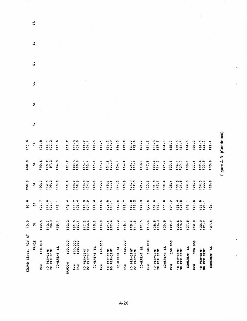
o

o o

o

o in

o

o

3 co — n o f»m<or~<-in«noiocnoTcocoi0r-cooco«u>n<0o*- C -"•••• ~

w ro T o ro ncor^i>Tco — —r-iomion — *-*-r-Tinin—TioTcoci c o «• O «- ooo—o — — no«- — n»-nnco*-confonconconn Q

" """ - - *"* " *" " " *" - - - *"" - - " - - " -- - - " ** O

°? IB ein e »locncoTOinoocnTncoi^coionnt'-ioooo — i io o> <T •!•••• • ^

m o o r- T — oininn«-*-*-r-TTToa>r-f~T»-coTocor~r~iOin CD o «- cr> o ooo—o — — non — n— «- — n— nnronronconco i- - - - - - .- - r- - - - .- .- .- .- - - - - - - »- - - ,- r- .- - .- 3

a> iZ

r- on to a> i- ro to m a> in co •- n a> oin i- r- o •- w — into co m oio in _j • > • > . in co «TO in CM CO CD co T O O air» T in mn «- o *• !«■ o in in»- * in «re» co

O «- O •- O OO .- O PI «- •■ O «- — n — CM CM CO «- CO CM DCM T CM CO n CM

r» o *- — T t- T cooi v io a>>- to t» OCM to 10 o— o o «in — to 01 *• •- _i • >- >

in r> vo CM co coco COT T — —co r» io i> co r» o «-I» o in in— o> co com m o »- o »- o oo — o CM »- no •- •- n — n n. co •- co n co n co n con ro »- — «- — — •— — — — — — •— •— — «— T— »- —' — W — — — — T- •" •■ — — «—

m i- en — M ia«- iniomo»—Tn — TiDin<oincoo>t~ion<oo>oir»in _j > •• • • m n no en n n c- i- co m o »- r» t- in in ■- •- t- IDV o n e* o> t- T n — r»

o —o> o o oo —o — — no — •- n — n — n — n n PI— n n con n

> UJ o o o o o o o o o u ID

z < o o

-j

o o

o o o o

_J

o o

_J

o o

—1

o o

-J

o o

-j

o o

_J • or o t- »- in o o o i- t- in o t- f- Ol o i- *- in o »- ►- m o »- »- in o »- t- m _J o z z o o n z z «r z z ID z z CO z z o z z n z z UJ *- UJ UJ t— V- «- v— UJ UJ f- *- UJ UJ »- v- UJ UJ »- r- UJ UJ i- n UJ UJ h- n UJ UJ t—

> UJ 1 1

z UJ 1 1

z UJ

u o 1 1

z UJ

<-> CJ 1 1

z UJ

u u 1 1

z UJ 1 1

Z UJ

(J U I 1

z UJ

-1 o- ir a a or tr or or or or or or or or or or or or or or or UJ UJ UJ UJ UJ UJ UJ UJ UJ UJ UJ UJ UJ UJ UJ UJ UJ UJ UJ Ul UJ

o a. a I 5 a. a I a. a I a a. T a a I a a I a. a. I z r O o X z O r n r n r o r O z O => x o o o Q X X o o u X o o u x o o o x o o u x o o o X o o Ü o a - o> z or or — 01 or — 0> or •- 0> or — 0> or - 01 or «- 01

A-20

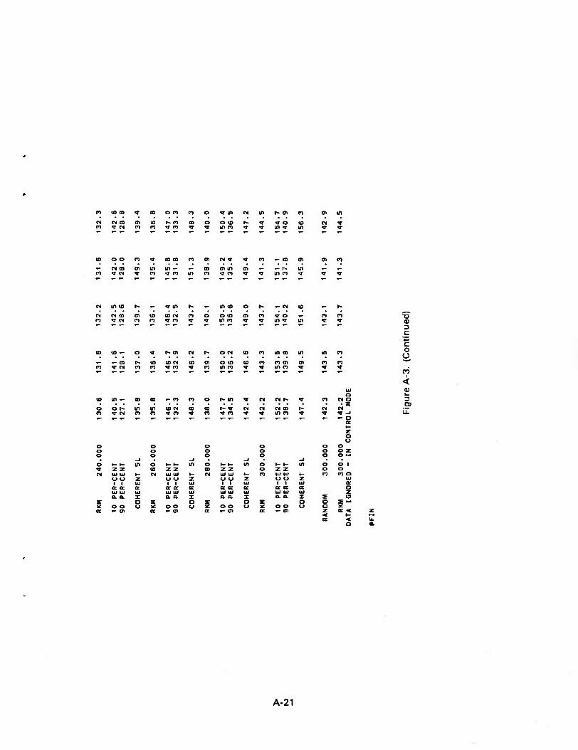
niD(BVO)omctoitinciint~(j\ri oil/)

CNCMC0 01UJt-rnCOOOlOr~>I«rO<0 CM «» n«T<Ntnp)«rr>«r«rinr)«r«tin«TU) T i

<ooop)q-oocopioicM««r>>-(DO> en m *- CMCO o>m m«- *-coo>in en *-»-r~ in •» *» co«j'CM«TC'j«*minr'><i-c>«»iino«* v «r

«<NcDaiiDiDcir)Oo(DCTir),*o»- nn ciTCMmp>>Tco«T«Tmr>«j«Tin«"'in i «r

« v<- o < t-oi N N on v n na u inn

*- «-co r- 10 ton to 01 010 u> ci root 01 n PI n in n n «n « n inn « v »n « •» •»

Ui a

10 tn<- 10 os — n n o t- in 1 en ON «T P» no • • z

oot-ininiccMODiot-'j-cMCMCMCot-- CM 01 m «T CM m n in «r n «TO «r «x inn «r «r «-1 .- — ,- .- - ,-.- .- .- »-.- .- .- »-.- »- «■ -~ o

1 .E c o o CO

I

< 0) k.

05

0 0

0 0 0 0 0 0 0 0 0 0 0 0 z 0

_i 0

_j 0

_i 0

-I 0 0 •-

0 t- (- in 0 ►- 1- in 0 1- t- m 0 1- 1- m 0 0 1 1 Z Z 10 z z CO z z 0 z z 0 0 CM uj ui h- CM UI UJ 1- CM UJ UI i- m uj ui ►- en p> 0

u u 1 1

Z UJ

0 <_> 1 1

z UJ

0 0 1 1

z UI

u 0 1 1

z UJ

UI cc

cr cr CC cc or a cc cr cr cc cc cc a uj UJ UJ UJ UI UI uj ui UJ UJ UJ UJ z a a. I a. 0. I 0. a I CL a. I I 0

I 0 2F O f 0 r 0 O X ~ IT 0 0 0 X 0 0 0 ■x. 0 0 (-> sr 0 0 u a X cc — o> ■r — o> cc — 01 cc •- o> z < cc <

A-21