asir - department of mathematics, kobe university · asir is a standard language interface of...
TRANSCRIPT
AsirAsir User’s Manual
Asir-20100206 (Kobe Distribution)February 2010
by Masayuki Noro, Takeshi Shimoyama, Taku Takeshimaand Risa/Asir committers

Copyright c⃝ FUJITSU LABORATORIES LIMITED. 1994-2000. All rights reserved.Copyright 2000-2010, Risa/Asir committers, http://www.openxm.org/.

Chapter 1: Introduction 1
1 Introduction
1.1 Organization of the Manual
This manual is organized as follows.
1. IntroductionOrganization of the Manual, notation and how to get Risa/Asir
2. Risa/AsirSummary of Asir, Installation
3. TypesTypes in Asir
4. Asir user languageDescription of Asir user language
5. DebuggerDescription of the debugger of Asir user language
6. Built-in functionDetailed description of various built-in functions
7. Distributed computationDescription of functions for distributed computation
8. Groebner basesDescription of functions and operations for Groebner basis computation
9. Algebraic numbersDescription of functions and operations for algebraic numbers
10. Finite fieldsDescription of functions and operations on finite fields
11. AppendixSyntax in detail, description of sample files, interfaces for input from keyboard, changes,references
1.2 Notation
In this manual, we shall use several notations, which is described here
• The name of a function is written in a typewriter typegcd(), gr()
• For the description of a function, its argument is written in a slanted type.
int, poly
• A file name is written in a ‘typewriter type with single quotes’‘dbxinit’, ‘asir_plot’
• An example is indented and written in a typewriter type.
[0] 1;1[1] quit;

Chapter 1: Introduction 2
• References are made by a typewriter type bracketed by [].[Boehm,Weiser]
• Arguments (actual parameters) of a function are optional when they are bracketedby []’s. The repeatable items (including non-existence of the item) are bracketed by[]*’s.setprec([n]), diff(rat[,varn]*)
• The prompt from the shell (csh) is denoted, as it is, by %. The prompt, however, isdenoted by #, when you are assumed to be working as the root, for example, at theinstallation.
% cat afoafobfo% suPassword:XXXX# cp asir /usr/local/bin# exit%
• The rational integer ring is denoted by Z, the rational number field by Q, the realnumber field by R, and the complex number field by C.
1.3 How to get Risa/Asir
The source code of Risa/Asir (‘asir2000.tgz’), PARI (‘pari.tgz’) and Windows binary(‘asirwin-ja.tgz’, ‘asirwin-en.tgz’) are available via ftp from
ftp://ftp.math.kobe-u.ac.jp/pub/asir

Chapter 2: Risa/Asir 3
2 Risa/Asir
2.1 Risa and Asir
Risa is the name of whole libraries of a computer algebra system which is under developmentat FUJITSU LABORATORIES LIMITED. The structure of Risa is as follows.
• The basic algebraic engineThis is the part which performs basic algebraic operations, such as arithmetic opera-tions, to algebraic objects, e.g., numbers and polynomials, which are already convertedinto internal forms. It exists, like ‘libc.a’ of UNIX, as a library of ordinary UNIXsystem. The algebraic engine is written mainly in C language and partly in assembler.It serves as the basic operation part of Asir, a standard language interface of Risa.
• Memory ManagerRisa employs, as its memory management component (the memory manager), a freesoftware distributed by Boehm (gc-6.1alpha5). It is proposed by [Boehm,Weiser],and developed by Boehm and his colleagues. The memory manager has a memoryallocator which automatically reclaims garbages, i.e., allocated but unused memories,and refreshes them for further use. The algebraic engine gets all its necessary memoriesthrough the memory manager.
• AsirAsir is a standard language interface of Risa’s algebraic engine. It is one of the possiblelanguage interfaces, because one can develop one’s own language interface easily on Risasystem. Asir is an example of such language interfaces. Asir has very similar syntaxand semantics as C language. Furthermore, it has a debugger that provide a subset ofcommands of dbx, a widely used debugger of C language.
2.2 Features of Asir
As mentioned in the previous section, Asir is a standard language interface forRisa’s al-gebraic engine. Usually, it is provided as an executable file named asir. Main featuressupported for the current version of Asir is as follows.
• A C-like programming language
• Arithmetic operations (addition, subtraction, multiplication and division) on numbers,polynomials and rational expressions
• Operations on vectors and matrices
• List processing operations at the minimum
• Several Built-in functions (factorization, GCD computation, Groebner basis computa-tion etc.)
• Useful user defined functions(e.g., factorization over algebraic number fields)
• A dbx-like debugger
• Plotting of implicit functions
• Numerical evaluation of mathematical expressions including elementary transcendentalfunctions at arbitrary precision. This feature is in force only if PARI system (seeSection 6.1.14 [pari], page 40).

Chapter 2: Risa/Asir 4
• Distributed computation over UNIX
2.3 Installation
Any questions and any comments on this manual are welcome by e-mails to the followingaddress.
2.3.1 UNIX binary version
A file ‘asir.tgz’ suitable for the target machine/architecture is required. After gettingit, you have to unpack it by gzip. First of all, determine a derectory where binaries andlibrary files are installed. We call the directory the library directory. The following installsthe files in ‘/usr/local/lib/asir’.
# gzip -dc asir.tgz | ( cd /usr/local/lib; tar xf - )
In this case you don’t have to set any environment variable.
You can install them elsewhere.
% gzip -dc asir.tgz | ( cd $HOME; tar xf - )
In this case you have to set the name of the library directory to the environment variableASIR_LIBDIR.
% setenv ASIR_LIBDIR $HOME/asir
Asir itself is in the library directory. It will be convenient to create a symbolic link to itfrom ‘/usr/local/bin’ or the user’s search path.
# ln -s /usr/local/lib/asir/asir /usr/local/bin/asir
Then you can start ‘asir’.
% /usr/local/bin/asirThis is Risa/Asir, Version 20000821.Copyright (C) FUJITSU LABORATORIES LIMITED.1994-2000. All rights reserved.[0]
2.3.2 UNIX source code version
First of all you have to determine the install directory. In the install directory, thefollowing subdirectories are put:
• bin
executables of PARI and Asir
• lib
library files of PARI and Asir
• include
header files of PARI
These subdirectories are created automatically if they does not exist. If you can be aroot, it is recommended to set the install directory to ‘/usr/local’. In the following thedirectory is denoted by TARGETDIR.
Then, install PARI library. After getting ‘pari.tgz’, unpack and install it as follows:

Chapter 2: Risa/Asir 5
% gzip -dc pari.tgz | tar xvf -% cd pari% ./Configure --prefix=TARGETDIR% make all% su# make install# make install-lib-sta
While executing ’make install’, the procedure may stop due to some error. Then try thefollowing:
% cd Oxxx% make lib-sta% su# make install-lib-sta# make install-include# exit%
In the above example, xxx denotes the name of the target operating system. AlthoughGP is not built, the library necessary for building asir2000 will be generated.
After getting ‘asir2000.tgz’, unpack it and install necessary files as follows.
% gzip -dc asir.tgz | tar xf -% cd asir2000% ./configure --prefix=TARGETDIR --with-pari --enable-plot% make% su# make install# make install-lib# make install-doc# exit
2.3.3 Windows version
The necessary file is ‘asirwin-en.tgz’. To unpack it ‘gzip.exe’ and ‘tar.exe’ are neces-sary. They are in the same directory as ‘asirwin-en.tgz’ on the ftp server. Putting themin the same directory, execute the following:
C:\...> tar xzf asirwin.tgz
Then a directory ‘Asir’ (Asir root directory) is created, which has subdirectories named‘bin’ and ‘lib’. Asir can be invoked by double-clicking ‘asirgui.exe’.
2.4 Command line options
Command-line options for the command ‘asir’ are as follows.
-heap numberIn Risa/Asir, 4KB is used as an unit, called block, for memory allocation. Bydefault, 16 blocks (64KB) are allocated initially. This value can be changedby giving an option -heap a number parameter in unit block. Size of the heaparea is obtained by a Built-in function heap(), the result of which is a numberin Bytes.

Chapter 2: Risa/Asir 6
-adj numberHeap area will be stretched by the memory manager, if the size of reclaimedmemories is less than 1/number of currently allocated heap area. The defaultvalue for number is 3. If you do not prefer to stretch heap area by some reason,perhaps by restriction of available memories, but if prefer to resort to reclaiminggarbages as far as possible, then a large value should be chosen for number, e.g.,8.
-norc When this option is specified, Asir does not read the initial file ‘$HOME/.asirrc’.
-quiet
-f file Instead of the standard input, file is used as the input. Upon an error, theexecution immediately terminates.
-paristack numberThis option specifies the private memory size for PARI (see Section 6.1.14 [pari],page 40). The unit is Bytes. By default, it is set to 1 MB.
-maxheap numberThis option sets an upper limit of the heap size. The unit is Bytes. Note thatthe size is already limited by the value of datasize displayed by the commandlimit on UNIX.
2.5 Environment variable
There exist several environment variables concerning with an execution of Asir. On UNIX,an environment variable is set from shells, or in rc files of shells. On Windows NT, itcan be set from [Control Panel] ->[Environment]. On Windows 95/98, it can be set in‘c:\autoexec.bat’. Note that the setting takes effect after rebooting the machine onWindows 95/98.
• ASIR_LIBDIR
The library directory of Asir, i.e., the directory where , for example, files containingprograms written in Asir. If not specified, on UNIX, ‘/usr/local/lib/asir’ is used bydefault. On Windows, ‘lib’ in Asir root directory is used by default. This environmentwill be useful in a case where Asir binaries are installed on a private directory of theuser. This environmental variable will become obsolete.
• ASIR_CONTRIB_DIR
The asir-contrib library directory of Asir, i.e., the directory where packages anddata developed by the OpenXM/asir-contrib project files are put. If not specified,on UNIX, ‘/usr/local/lib/asir-contrib’ is used by default. On Windows,‘lib-asir-contrib’ in Asir root directory is used by default. This environment willbe useful in a case where Asir binaries are installed on a private directory of the user.
• ASIRLOADPATH
This environment specifies directories which contains files to be loaded by Asir com-mand load(). Directories are separated by a ‘:’ on UNIX, a ’;’ on Windows respec-tively. The search order is from the left to the right. After searching out all directoriesin ASIRLOADPATH, or in case of no specification at all, the library directory will besearched.

Chapter 2: Risa/Asir 7
• HOME
If Asir is invoked without -norc, ‘$HOME/.asirrc’, if exists, is executed. If HOME isnot set, nothing is done on UNIX. On Windows, ‘.asirrc’ in Asir root directory isexecuted if it exists.
2.6 Starting and Terminating an Asir session
Run Asir, then the copyright notice and the first prompt will appear on your screen, and anew Asir session will be started.
[0]
When initialization file ‘$HOME/.asirrc’ exists, Asir interpreter executes it at first takingit as a program file written in Asir.
The prompt indicates the sequential number of your input commands to Asir. The sessionwill terminate when you input end; or quit; to Asir. Input commands are evaluatedstatement by statement. A statement normally ends with its terminator ‘;’ or ‘$’. (Thereare some exceptions. See, syntax of Asir.) The result will be displayed when the command,i.e. statement, is terminated by a ‘;’, and will not when terminated by a ‘$’.
% asir[0] A;0[1] A=(x+y)^5;x^5+5*y*x^4+10*y^2*x^3+10*y^3*x^2+5*y^4*x+y^5[2] A;x^5+5*y*x^4+10*y^2*x^3+10*y^3*x^2+5*y^4*x+y^5[3] a=(x+y)^5;evalpv : invalid assignmentreturn to toplevel[3] a;a[4] fctr(A);[[1,1],[x+y,5]][5] quit;%
In the above example, names A, a, x and y are used to identify mathematical and program-ming objects. There, the name A denotes a program variable (some times called simply as aprogram variable.) while the other names, a, x and y, denote mathematical objects, that is,indeterminates. In general, program variables have names which begin with capital letters,while names of indeterminates begin with small letters. As you can see in the example,program variables are used to hold and keep objects, such as numbers and expressions,as their values, just like variables in C programming language. Whereas, indeterminatescannot have values so that assignment to indeterminates are illegal. If one wants to get aresult by substituting a value for an indeterminate in an expression, it is achieved by thefunction subst as the value of the function.

Chapter 2: Risa/Asir 8
2.7 Interruption
To interrupt the Asir execution, input an interrupt character from the keyboard. A C-c isusually used for it. (Notice: C-x on Windows and DOS.)
@ (x+y)^1000;C-cinterrupt ?(q/t/c/d/u/w/?)
Here, the meaning of options are as follows.
q Terminates Asir session. (Confirmation requested.)
t Returns to toplevel. (Confirmation requested.)
c Resumes to continue the execution.
d Enters debugging mode at the next statement of the Asir program, if Asirhas been executing a program loaded from a file. Note that it will sometimestake a long time before entering debugging mode when Asir is executing basicfunctions in the algebraic engine, (e.g., arithmetic operation, factorization etc.)Detailed description about the debugger will be given in Chapter 5 [Debugger],page 30.
u After executing a function registered by register_handler() (see Section 7.5.6[ox reset ox intr register handler], page 107), returns to toplevel. A confirma-tion is prompted.
w Displays the calling sequence up to the interruption.
? Show a brief description of options.
2.8 Error handling
When arguments with illegal types are given to a built-in function, an error will be detectedand the execution will be quit. In many cases, when an error is detected in a built-infunction, Asir automatically enters debugging mode before coming back to toplevel. Atthat time, one can examine the state of the program, for example, inspect argument valuesjust before the error occurred. Messages reported there are various depending on cases.They are reported after the internal function name. The internal function name sometimesdiffers from the built-in function name that is specified by the user program.
In the execution of internal functions, errors may happen by various reasons. The UNIXversion of Asir will report those errors as one of the following internal error’s, and entersdebugging mode just like normal errors.
SEGV
BUS ERROR
Some of the built-in functions transmit their arguments to internal operationroutines without strict type-checking. In such cases, one of these two errors willbe reported when an access violation caused by an illegal pointer or a NULLpointer is detected.
BROKEN PIPE
In the process communication, this error will be reported if a process attempts

Chapter 2: Risa/Asir 9
to read from or to write onto the partner process when the stream to the partnerprocess does not already exist, (e.g., terminated process.)
For UNIX version, even in such a case, the process itself does not terminate because suchan error can be caught by signal() and recovered. To remove this weak point, completetype checking of all arguments are indispensable at the entry of a built-in function, whichrequires an enormous amount of re-making efforts.
2.9 Referencing results and special numbers
An @ used for an escape character; rules currently in force are as follows.
@n The evaluated result of n-th input command
@@ The evaluated result of the last command
@i The unit of imaginary number, square root of -1.
@pi The number pi, the ratio of a circumference of the circle and its diameter.
@e Napier’s number, the base of natural logarithm.
@ A generator of GF(2^m), a finite field of characteristic 2, over GF(2). It isa root of an irreducible univariate polynomial over GF(2) which is set as thedefining polynomial of GF(2^m).
@>, @<, @>=, @<=, @==, @&&, @||
Fist order logical operators. They are used in quantifier elimination.
[0] fctr(x^10-1);[[1,1],[x-1,1],[x+1,1],[x^4+x^3+x^2+x+1,1],[x^4-x^3+x^2-x+1,1]][1] @@[3];[x^4+x^3+x^2+x+1,1][2] eval(sin(@pi/2));1.000000000000000000000000000000000000000000000000000000000[3] eval(log(@e),20);0.99999999999999999999999999998[4] @0[4][0];x^4-x^3+x^2-x+1[5] (1+@i)^5;(-4-4*@i)[6] eval(exp(@pi*@i));-1.0000000000000000000000000000[7] (@+1)^9;(@^9+@^8+@+1)
As you can see in the above example, results of toplevel computation can be referred to by@ convention. This is convenient for users, while it sometimes imposes a heavy burden tothe garbage collector. It may happen that GC time will rapidly increase after computing avery large expression at the toplevel. In such cases delete_history() (see Section 6.14.15[delete_history], page 97) takes effect.

Chapter 3: Data types 10
3 Data types
3.1 Types in Asir
In Asir, various objects described according to the syntax of Asir are translated to in-termediate forms and by Asir interpreter further translated into internal forms with thehelp of basic algebraic engine. Such an object in an internal form has one of the followingtypes listed below. In the list, the number coincides with the value returned by the built-infunction type(). Each example shows possible forms of inputs for Asir’s prompt.
0 0As a matter of fact, no object exists that has 0 as its identification number. Thenumber 0 is implemented as a null (0) pointer of C language. For convenience’ssake, a 0 is returned for the input type(0).
1 number
1 2/3 14.5 3+2*@i
Numbers have sub-types. See Section 3.2 [Types of numbers], page 13.
2 polynomial (but not a number)x afo (2.3*x+y)^10
Every polynomial is maintained internally in its full expanded form, representedas a nested univariate polynomial, according to the current variable ordering,arranged by the descending order of exponents. (See Section 8.1 [Distributedpolynomial], page 118.) In the representation, the indeterminate (or variable),appearing in the polynomial, with maximum ordering is called the main vari-able. Moreover, we call the coefficient of the maximum degree term of thepolynomial with respect to the main variable the leading coefficient.
3 rational expression (not a polynomial)(x+1)/(y^2-y-x) x/x
Note that in Risa/Asir a rational expression is not simplified by reducing thecommon divisors unless red() is called explicitly, even if it is possible. This isbecause the GCD computation of polynomials is a considerably heavy opera-tion. You have to be careful enough in operating rational expressions.
4 list
[] [1,2,[3,4],[x,y]]
Lists are all read-only object. A null list is specified by []. There are operationsfor lists: car(), cdr(), cons() etc. And further more, element referencing byindexing is available. Indexing is done by putting [index]’s after a programvariable as many as are required. For example,
[0] L = [[1,2,3],[4,[5,6]],7]$[1] L[1][1];[5,6]
Notice that for lists, matrices and vectors, the index begins with number 0.Also notice that referencing list elements is done by following pointers from

Chapter 3: Data types 11
the first element. Therefore, it sometimes takes much more time to performreferencing operations on a large list than on a vectors or a matrices with thesame size.
5 vector
newvect(3) newvect(2,[a,1])
Vector objects are created only by explicit execution of newvect() command.The first example above creates a null vector object with 3 elements. The otherexample creates a vector object with 2 elements which is initialized such thatits 0-th element is a and 1st element is 1. The second argument for newvect isused to initialize elements of the newly created vector. A list with size smalleror equal to the first argument will be accepted. Elements of the initializing listis used from the left to the right. If the list is too short to specify all the vectorelements, the unspecified elements are filled with as many 0’s as are required.Any vector element is designated by indexing, e.g., [index]. Asir allows anytype, including vector, matrix and list, for each respective element of a vector.As a matter of course, arrays with arbitrary dimensions can be representedby vectors, because each element of a vector can be a vector or matrix itself.An element designator of a vector can be a left value of assignment statement.This implies that an element designator is treated just like a simple programvariable. Note that an assignment to the element designator of a vector haseffect on the whole value of that vector.
[0] A3 = newvect(3);[ 0 0 0 ][1] for (I=0;I<3;I++)A3[I] = newvect(3);[2] for (I=0;I<3;I++)for(J=0;J<3;J++)A3[I][J]=newvect(3);[3] A3;[ [ [ 0 0 0 ] [ 0 0 0 ] [ 0 0 0 ] ][ [ 0 0 0 ] [ 0 0 0 ] [ 0 0 0 ] ][ [ 0 0 0 ] [ 0 0 0 ] [ 0 0 0 ] ] ][4] A3[0];[ [ 0 0 0 ] [ 0 0 0 ] [ 0 0 0 ] ][5] A3[0][0];[ 0 0 0 ]
6 matrix
newmat(2,2) newmat(2,3,[[x,y],[z]])
Like vector objects, matrix objects are also created only by explicit execution ofnewmat() command. Initialization of the matrix elements are done in a similarmanner with that of the vector elements except that the elements are specifiedby a list of lists. Each element, again a list, is used to initialize each row; if thelist is too short to specify all the row elements, unspecified elements are filledwith as many 0’s as are required. Like vectors, any matrix element is designatedby indexing, e.g., [index][index]. Asir also allows any type, including vector,matrix and list, for each respective element of a matrix. An element designatorof a matrix can also be a left value of assignment statement. This implies thatan element designator is treated just like a simple program variable. Note thatan assignment to the element designator of a matrix has effect on the whole

Chapter 3: Data types 12
value of that matrix. Note also that every row, (not column,) of a matrix canbe extracted and referred to as a vector.
[0] M=newmat(2,3);[ 0 0 0 ][ 0 0 0 ][1] M[1];[ 0 0 0 ][2] type(@@);5
7 string
"" "afo"
Strings are used mainly for naming files. It is also used for giving commentsof the results. Operator symbol + denote the concatenation operation of twostrings.
[0] "afo"+"take";afotake
8 structurenewstruct(afo)
The type structure is a simplified version of that in C language. It is definedas a fixed length array and each entry of the array is accessed by its name. Aname is associated with each structure.
9 distributed polynomial2*<<0,1,2,3>>-3*<<1,2,3,4>>
This is the short for ‘Distributed representation of polynomials.’ This typeis specially devised for computation of Groebner bases. Though for ordinaryusers this type may never be needed, it is provided as a distinguished type thatuser can operate by Asir. This is because the Groebner basis package providedwith Risa/Asir is written in the Asir user language. For details See Chapter 8[Groebner basis computation], page 118.
10 32bit unsigned integer
11 error object
These are special objects used for OpenXM.
12 matrix over GF(2)
This is used for basis conversion in finite fields of characteristic 2.
13 MATHCAP object
This object is used to express available funcionalities for Open XM.
14 first order formula
This expresses a first order formula used in quantifier elimination.

Chapter 3: Data types 13
15 matrix over GF(p)
A matrix over a small finite field.
16 byte array
An array of unsigned bytes.
-1 VOID object
The object with the object identifier -1 indicates that a return value of a functionis void.
3.2 Types of numbers
0 rational numberRational numbers are implemented by arbitrary precision integers (bignum). Arational number is always expressed by a fraction of lowest terms.
1 double precision floating point number (double float)The numbers of this type are numbers provided by the computer hardware. Bydefault, when Asir is started, floating point numbers in a ordinary form aretransformed into numbers of this type. However, they will be transformed intobigfloat numbers when the switch bigfloat is turned on (enabled) by ctrl()
command.
[0] 1.2;1.2[1] 1.2e-1000;0[2] ctrl("bigfloat",1);1[3] 1.2e-1000;1.20000000000000000513 E-1000
A rational number shall be converted automatically into a double float numberbefore the operation with another double float number and the result shall becomputed as a double float number.
2 algebraic numberSee Chapter 9 [Algebraic numbers], page 152.
3 bigfloatThe bigfloat numbers of Asir is realized by PARI library. A bigfloat numberof PARI has an arbitrary precision mantissa part. However, its exponent partadmits only an integer with a single word precision. Floating point operationswill be performed all in bigfloat after activating the bigfloat switch by ctrl()
command. The default precision is about 9 digits, which can be specified bysetprec() command.
[0] ctrl("bigfloat",1);1

Chapter 3: Data types 14
[1] eval(2^(1/2));1.414213562373095048763788073031[2] setprec(100);9[3] eval(2^(1/2));1.41421356237309504880168872420969807856967187537694807317...
Function eval() evaluates numerically its argument as far as possible. Noticethat the integer given for the argument of setprec() does not guarantee theaccuracy of the result, but it indicates the representation size of numbers withwhich internal operations of PARI are performed. (See Section 6.1.13 [evaldeval], page 39, Section 6.1.14 [pari], page 40.)
4 complex numberA complex number of Risa/Asir is a number with the form a+b*@i, where @i isthe unit of imaginary number, and a and b are either a rational number, doublefloat number or bigfloat number, respectively. The real part and the imaginarypart of a complex number can be taken out by real() and imag() respectively.
5 element of a small finite prime fieldHere a small finite fieid means that its characteristic is less than 2^27. Atpresent small finite fields are used mainly for groebner basis computation, andelements in such finite fields can be extracted by taking coefficients of dis-tributed polynomials whose coefficients are in finite fields. Such an elementitself does not have any information about the field to which the element be-longs, and field operations are executed by using a prime p which is set bysetmod().
6 element of large finite prime fieldThis type expresses an element of a finite prime field whose characteristic is anarbitrary prime. An object of this type is obtained by applying simp_ff to aninteger.
7 element of a finite field of characteristic 2This type expresses an element of a finite field of characteristic 2. Let F be afinite field of characteristic 2. If [F:GF(2)] is equal to n, then F is expressed asF=GF(2)[t]/(f(t)), where f(t) is an irreducible polynomial over GF(2) of degreen. As an element g of GF(2)[t] can be expressed by a bit string, An element gmod f in F can be expressed by two bit strings representing g and f respectively.
Several methods to input an element of F are provided.
• @
@ represents t mod f in F=GF(2)[t](f(t)). By using @ one can input anelement of F. For example @^10+@+1 represents an element of F.
• ptogf2n
ptogf2n converts a univariate polynomial into an element of F.
• ntogf2n
As a bit string, a non-negative integer can be regarded as an element ofF. Note that one can input a non-negative integer in decimal, hexadecimal(0x prefix) and binary (0b prefix) formats.

Chapter 3: Data types 15
• micellaneous
simp_ff is available if one wants to convert the whole coefficients of apolynomial.
8 element of a finite field of characteristic p^n
A finite field of order p^n, where p is an arbitrary prime and n is a positiveinteger, is set by setmod_ff by specifying its characteristic p and an irreduciblepolynomial of degree n over GF(p). An element of this field is represented bya polynomial over GF(p) modulo m(x).
9 element of a finite field of characteristic p^n (small order)
A finite field of order p^n, where p^n must be less than 2^29 and n must beequal to 1 if p is greater or equal to 2^14, is set by setmod_ff by specifyingits characteristic p the extension degree n. If p is less than 2^14, each non-zeroelement of this field is a power of a fixed element, which is a generator of themultiplicative group of the field, and it is represented by its exponent. Other-wise, each element is represented by the redue modulo p. This specification isuseful for treating both cases in a single program.
10 element of a finite field which is an algebraic extension of a small finite field ofcharacteristic p^n
An extension field K of the small finite field F of order p^n is set by setmod_
ff by specifying its characteristic p the extension degree n and m=[K :F]. Anirreducible polynomial of degree m over K is automatically generated and usedas the defining polynomial of the generator of the extension K/F. The generatoris denoted by @s.
11 algebraic number represented by a distributed polynomialSee Chapter 9 [Algebraic numbers], page 152.
Finite fields other than small finite prime fields are set by setmod_ff. Elements of finitefields do not have informations about the modulus. Upon an arithmetic operation, i f oneof the operands is a rational number, it is automatically converted into an element of thefinite field currently set and the operation is done in the finite field.
3.3 Types of indeterminates
An algebraic object is recognized as an indeterminate when it can be a (so-called) variablein polynomials. An ordinary indeterminate is usually denoted by a string that start with asmall alphabetical letter followed by an arbitrary number of alphabetical letters, digits or‘_’. In addition to such ordinary indeterminates, there are other kinds of indeterminates ina wider sense in Asir. Such indeterminates in the wider sense have type polynomial, andfurther are classified into sub-types of the type indeterminate.
0 ordinary indeterminateAn object of this sub-type is denoted by a string that start with a small al-phabetical letter followed by an arbitrary number of alphabetical letters, digitsor ‘_’. This kind of indeterminates are most commonly used for variables ofpolynomials.

Chapter 3: Data types 16
[0] [vtype(a),vtype(aA_12)];[0,0]
1 undetermined coefficientThe function uc() creates an indeterminate which is denoted by a string thatbegins with ‘_’. Such an indeterminate cannot be directly input by its name.Other properties are the same as those of ordinary indeterminate. Therefore,it has a property that it cannot cause collision with the name of ordinaryindeterminates input by the user. And this property is conveniently used tocreate undetermined coefficients dynamically by programs.
[1] U=uc();_0[2] vtype(U);1
2 function formA function call to a built-in function or to an user defined function is usuallyevaluated by Asir and retained in a proper internal form. Some expressions,however, will remain in the same form after evaluation. For example, sin(x)and cos(x+1) will remain as if they were not evaluated. These (unevaluated)forms are called ‘function forms’ and are treated as if they are indeterminatesin a wider sense. Also, special forms such as @pi the ratio of circumference anddiameter, and @e Napier’s number, will be treated as ‘function forms.’
[3] V=sin(x);sin(x)[4] vtype(V);2[5] vars(V^2+V+1);[sin(x)]
3 functorA function call (or a function form) has a form fname(args). Here, fname aloneis called a functor. There are several kinds of functors: built-in functor, userdefined functor and functor for the elementary functions. A functor alone istreated as an indeterminate in a wider sense.
[6] vtype(sin);3

Chapter 4: User language Asir 17
4 User language Asir
Asir provides many built-in functions, which perform algebraic computations, e.g., factor-ization and GCD computation, file I/O, extract a part of an algebraic expression, etc. Inpractice, you will often encounter a specific problem for which Asir does not provide a directsolution. For such cases, you have to write a program in a certain user language. The userlanguage for Asir is also called Asir. In the following, we describe the Syntax and thenshow how to write a user program by several examples.
4.1 Syntax — Difference from C language
The syntax of Asir is based on C language. Main differences are as follows. In this section,a variable does not mean an indeterminate, but a program variable which is written by astring which begins with a capital alphabetical letter in Asir.
• No types for variables.As is already mentioned, any object in Asir has their respective types. A programvariable, however, is type-less, that is, any typed object can be assigned to it.
[0] A = 1;1[1] type(A);1[2] A = [1,2,3];[1,2,3][3] type(A);4
• Variables, together with formal parameters, in a function (procedure) are all local tothe function by default.Variables can be global at the top level, if they are declared with the key word extern.Thus, the scope rule of Asir is very simple. There are only two types of variables:global variables and local variables. A name that is input to the Asir’s prompt at thetop level is denotes a global variable commonly accessed at the top level. In a function(procedure) the following rules are applied.
1. If a variable is declared as global by an extern statement in a function, the variableused in that function denotes a global variable at the top level. Furthermore, if avariable in a function is preceded by an extern declaration outside the functionbut in a file where the function is defined, all the appearance of that variable inthe same file denote commonly a global variable at the top level.
2. A variable in a function is local to that function, if it is not declared as global byan extern declaration.
% cat afodef afo() { return A;}extern A$def bfo() { return A;}end$% asir[0] load("afo")$

Chapter 4: User language Asir 18
[5] A = 1;1[6] afo();0[7] bfo();1
• Program variables and algebraic indeterminates are distinguished in Asir.The names of program variables must begin with a capital letter; while the names ofindeterminates and functions must begin with a small letter.
This is an unique point that differs from almost all other existing computer algebrasystems. The distinction between program variables and indeterminates is adopted toavoid the possible and usual confusion that may arise in a situation where a name isused as an indeterminate but, as it was, the name has been already assigned somevalue. To use different type of letters, capital and small, was a matter of syntacticalconvention like Prolog, but it is convenient to distinguish variables and indeterminatesin a program.
• No switch statements, and goto statements.Lack of goto statement makes it rather bothering to exit from within multiple loops.
• Comma expressions are allowed only in A, B and C of the constructs for (A;B;C) orwhile(A).This limitation came from adopting lists as legal data objects for Asir.
The above are limitations; extensions are listed as follows.
• Arithmetic for rational expressions can be done in the same manner as is done fornumbers in C language.
• Lists are available for data objects.
Lists are conveniently used to represent a certain collection of objects. Use of listsenables to write programs more easily, shorter and more comprehensible than use ofstructure like C programs.
• Options can be specified in calling user defined functions.
See Section 4.2.12 [option], page 26.
4.2 Writing user defined functions
4.2.1 User defined functions
To define functions by an user himself, ‘def’ statement must be used. Syntactical errors aredetected in the parsing phase of Asir, and notified with an indication of where Asir foundthe error. If a function with the same name is already defined (regardless to its arity,) thenew definition will override the old one, and the user will be told by a message,
afo() redefined.
on the screen when a flag verbose is set to a non-zero value by ctrl(). Recursive definition,and of course, recursive use of functions are available. A call for an yet undefined functionin a function definition is not detected as an error. An error will be detected at executionof the call of that yet undefined function.

Chapter 4: User language Asir 19
/* X! */
def f(X) {if ( !X )
return 1;else
return X * f(X-1);}
/* iCj ( 0 ≤ i ≤ N, 0 ≤ j ≤ i ) */
def c(N){
A = newvect(N+1); A[0] = B = newvect(1); B[0] = 1;for ( K = 1; K <= N; K++ ) {
A[K] = B = newvect(K+1); B[0] = B[K] = 1;for ( P = A[K-1], J = 1; J < K; J++ )
B[J] = P[J-1]+P[J];}
return A;}
/* A+B */
def add(A,B)"add two numbers."{
return A+B;}
In the second example, c(N) returns a vector, say A, of length N+1. A[I] is a vector oflength I+1, and each element is again a vector which contains ICJ as its elements.
References
Section 6.14.4 [help], page 91.
In the following, the manner of writing Asir programs is exhibited for those who have noexperience in writing C programs.
4.2.2 variables and indeterminates
variables (program variables)A program variable is a string that begins with a capital alphabetical letterfollowed by any numbers of alphabetical letters, digits and ‘_’.
A program variable is thought of a box (a carrier) which can contain Asirobjects of various types. The content is called the ‘value’ of that variable.When an expression in a program is to be evaluated, the variable appearing in

Chapter 4: User language Asir 20
the expression is first replaced by its value and then the expression is evaluatedto some value and stored in the memory. Thus, no program variable appearsin objects in the internal form. All the program variables are initialized to thevalue 0.
[0] X^2+X+1;1[1] X=2;2[2] X^2+X+1;7
indeterminatesAn indeterminate is a string that begins with a small alphabetical letter followedby any numbers of alphabetical letters, digits and ‘_’.
An indeterminate is a transcendental element, so-called variable, which is usedto construct polynomial rings. An indeterminate cannot have any value. Noassignment is allowed to it.
[3] X=x;x[4] X^2+X+1;x^2+x+1[5] A=’Dx’*(x-1)+x*y-y;(y+Dx)*x-y-Dx[6] function foo(x,y);[7] B=foo(x,y)*x^2-1;foo(x,y)*x^2-1
4.2.3 parameters and arguments
def sum(N) {for ( I = 1, S = 0; I <= N; I++ )
S += I;return S;
}
This is an example definition of a function that sums up integers from 1 to N. The N insum(N) is called the (formal) parameter of sum(N). The example shows a function of thesingle argument. In general, any number of parameters can be specified by separating bycommas (‘,’). A (formal) parameter accepts a value given as an argument (or an actualparameter) at a function call of the function. Since the value of the argument is given to theformal parameter, any modification to the parameter does not usually affect the argument(or actual parameter). However, there are a few exceptions: vector arguments and matrixarguments.
Let A be a program variable and assigned to a vector value [ a, b ]. If A is given asan actual parameter to a formal parameter, say V, of a function, then an assignment in thefunction to the vector element designator V[1], say V[1]=c;, causes modification of theactual parameter A resulting A to have an altered value [ a c ]. Thus, if a vector is givento a formal parameter of a function, then its element (and subsequently the vector itself)in the calling side is modified through modification of the formal parameter by a vector

Chapter 4: User language Asir 21
element designator in the called function. The same applies to a matrix argument. Notethat, even in such case where a vector (or a matrix) is given to a formal parameter, theassignment to the whole parameter itself has only a local effect within the function.
def clear_vector(M) {/* M is expected to be a vector */L = size(M)[0];for ( I = 0; I < L; I++ )
M[I] = 0;}
This function will clear off the vector given as its argument to the formal parameter M andreturn a 0 vector.
Passing a vector as an argument to a function enables returning multiple results bypacking each result in a vector element. Another alternative to return multiple results is touse a list. Which to use depends on cases.
4.2.4 comments
The text enclosed by ‘/*’ and ‘*/’ (containing ‘/*’ and ‘*/’) is treated as a comment andhas no effect to the program execution as in C programs.
/** This is a comment.*/
def afo(X) {
A comment can span to several lines, but it cannot be nested. Only the first ‘/*’ is effectiveno matter how many ‘/*’’s in the subsequent text exist, and the comment terminates atthe first ‘*/’.
In order to comment out a program part that may contain comments in it, use the pair,#if 0 and #endif. (See Section 4.2.11 [preprocessor], page 25.)
#if 0def bfo(X) {/* empty */}#endif
4.2.5 statements
An user function of Asir is defined in the following form.
def name(parameter, parameter,...,parameter) {statementstatement...statement
}
As you can see, the statement is a fundamental element of the function. Therefore, in orderto write a program, you have to learn what the statement is. The simplest statement is thesimple statement. One example is an expression with a terminator (‘;’ or ‘$’.)

Chapter 4: User language Asir 22
S = sum(N);
A ‘return statement’ and ‘break statement’ are also primitives to construct ‘statements.’As you can see the syntactic definition of ‘if statement’ and ‘for statement’, each of theirbodies consists of a single ‘statement.’ Usually, you need several statements in such abody. To solve this contradictory requirement, you may use the ‘compound statement.’ A‘compound statement’ is a sequence of ‘statement’s enclosed by a left brace ‘{’ and a rightbrace ‘}’. Thus, you can use multiple statement as if it were a single statement.
if ( I == 0 ) {J = 1;K = 2;L = 3;
}
No terminator symbol is necessary after ‘}’, because ‘{’ statement sequence ‘}’ alreadyforms a statement, and it satisfies the syntactical requirement of the ‘if statement.’
4.2.6 return statement
There are two forms of return statement.
return expression;
return;
Both forms are used for exiting from a function. The former returns the value of theexpression as a function value. The function value of the latter is not defined.
4.2.7 if statement
There are two forms of if statement.
if ( expression ) if ( expression )statement and statement
elsestatement
The interpretation of these forms are obvious. However, be careful when another if state-ment comes at the place for ‘statement’. Let us examine the following example.
if ( expression1 )if ( expression2 ) statement1
elsestatement2
One might guess statement2 after else corresponds with the first if ( expression1 )
by its appearance of indentation. But, as a matter of fact, the Asir parser decides thatit correspond with the second if ( expression2 ). Ambiguity due to such two kinds offorms of if statement is thus solved by introducing a rule that a statement preceded by anelse matches to the nearest preceding if.
Therefore, rearrangement of the above example for improving readability according tothe actual interpretation gives the following.
if ( expression1 ) {if ( expression2 ) statement1 else statement2

Chapter 4: User language Asir 23
}
On the other hand, in order to reflect the indentation, it must be written as the following.
if ( expression1 ) {if ( expression2 ) statement1
} elsestatement2
When if is used in the top level, the if expression should be terminated with $ or ;. Ifthere is no terminator, the next expression will be skipped to be evaluated.
4.2.8 loop, break, return, continue
There are three kinds of statements for loops (repetitions): the while statement, the for
statement, and the do statement.
• while statementIt has the following form.
while ( expression ) statement
This statement specifies that statement is repeatedly evaluated as far as theexpression evaluates to a non-zero value. If the expression 1 is given to theexpression, it forms an infinite loop.
• for statementIt has the following form.
for ( expr list-1; expr; expr list-2 ) statement
This is equivalent to the program
expr list-1 (transformed into a sequence of simple statement)while ( expr ) {
statementexpr list-2 (transformed into a sequence of simple statement)
}
• do statement
do {statement
} while ( expression )
This statement differs from while statement by the location of the termination condi-tion: This statement first execute the statement and then check the condition, whereaswhile statement does it in the reverse order.
As means for exiting from loops, there are break statement and return statement. Thecontinue statement allows to move the control to a certain point of the loop.
• break
The break statement is used to exit the inner most loop.
• return
The return statement is usually used to exit from a function call and it is also effectivein a loop.

Chapter 4: User language Asir 24
• continue
The continue statement is used to move the control to the end point of the loop body.For example, the last expression list will be evaluated in a for statement, and thetermination condition will be evaluated in a while statement.
4.2.9 structure definition
A structure data type is a fixed length array and each component of the array is accessedby its name. Each type of structure is distinguished by its name. A structure data typeis declared by struct statement. A structure object is generated by a builtin functionnewstruct. Each member of a structure is accessed by an operatator ->. If a member of astructure is again a structure, then the specification by -> can be nested.
[1] struct rat {num,denom};0[2] A = newstruct(rat);{0,0}[3] A->num = 1;1[4] A->den = 2;2[5] A;{1,2}[6] struct_type(A);1
References
Section 6.7.1 [newstruct], page 71, Section 6.7.3 [struct_type], page 74
4.2.10 various expressions
Major elements to construct expressions are the following:
• addition, subtraction, multiplication, division, exponentiationThe exponentiation is denoted by ‘^’. (This differs from C language.) Division denotedby ‘/’ is used to operate in a field, for example, 2/3 results in a rational number 2/3. Forinteger division and polynomial division, both including remainder operation, built-infunctions are provided.
x+1 A^2*B*afo X/3
• programming variables with indicesAn element of a vector, a matrix or a list can be referred to by indexing. Note that theindices begin with number 0. When the referred element is again a vector, a matrix ora list, repeated indexing is also effective.
V[0] M[1][2]
• comparison operationThere are comparison operations ‘==’ for equivalence, ‘!=’ for non-equivalence, ‘>’,‘<’,‘>=’, and ‘<=’ for larger or smaller. The results of these operations are either value1 for the truth, or 0 for the false.

Chapter 4: User language Asir 25
• logical expressionThere are two binary logical operations ‘&&’ for logical ‘conjunction’(and), ‘||’ for log-ical ‘disjunction’(or), and one unary logical operation ‘!’ for logical ‘negation’(not).The results of these operations are either value 1 for the truth, and 0 for the false.
• assignmentValue assignment of a program variable is usually done by ‘=’. There are specialassignments combined with arithmetic operations. (‘+=’, ‘-=’, ‘*=’, ‘/=’, ‘^=’)
A = 2 A *= 3 (the same as A = A*3; The others are alike.)
• function callA function call is also an expression.
• ‘++’, ‘--’These operators are attached to or before a program variable, and denote special op-erations and values.
A++ the expression value is the previous value of A, and A = A+1A-- the expression value is the previous value of A, and A = A-1++A A = A+1, and the value is the one after increment of A--A A = A-1, and the value is the one after decrement of A
4.2.11 preprocessor
he Asir user language imitates C language. A typical features of C language include macroexpansion and file inclusion by the preprocessor cpp. Also, Asir read in user program filesthrough cpp. This enables Asir user to use #include, #define, #if etc. in his programs.
• #include
Include files are searched within the same directory as the file containing #include sothat no arguments are passed to cpp.
• #define
This can be used just as in C language.
• #if
This is conveniently used to comment out a large part of a user program that maycontain comments by /* and */, because such comments cannot be nested.
the following are the macro definitions in ‘defs.h’.
#define ZERO 0#define NUM 1#define POLY 2#define RAT 3#define LIST 4#define VECT 5#define MAT 6#define STR 7#define N_Q 0#define N_R 1#define N_A 2#define N_B 3#define N_C 4#define V_IND 0

Chapter 4: User language Asir 26
#define V_UC 1#define V_PF 2#define V_SR 3#define isnum(a) (type(a)==NUM)#define ispoly(a) (type(a)==POLY)#define israt(a) (type(a)==RAT)#define islist(a) (type(a)==LIST)#define isvect(a) (type(a)==VECT)#define ismat(a) (type(a)==MAT)#define isstr(a) (type(a)==STR)#define FIRST(L) (car(L))#define SECOND(L) (car(cdr(L)))#define THIRD(L) (car(cdr(cdr(L))))#define FOURTH(L) (car(cdr(cdr(cdr(L)))))#define DEG(a) deg(a,var(a))#define LCOEF(a) coef(a,deg(a,var(a)))#define LTERM(a) coef(a,deg(a,var(a)))*var(a)^deg(a,var(a))#define TT(a) car(car(a))#define TS(a) car(cdr(car(a)))#define MAX(a,b) ((a)>(b)?(a):(b))
Since we are utilizing the C preprocessor, it cannot properly preprocess expressions with $.For example, even if LIST is defined, LIST in the expression LIST$ is not replaced. Add ablank before $, i.e., write as LIST $ to make the proprocessor replace it properly.
4.2.12 option
If a user defined function is declared with N arguments, then the function is callablewith N arguments only.
[0] def factor(A) { return fctr(A); }[1] factor(x^5-1,3);evalf : argument mismatch in factor()return to toplevel
A function with indefinite number of arguments can be realized by using a list or anarray as its argument. Another method is available as follows:
% cat factordef factor(F){
Mod = getopt(mod);ModType = type(Mod);if ( ModType == 1 ) /* ’mod’ is not specified. */
return fctr(F);else if ( ModType == 0 ) /* ’mod’ is a number */
return modfctr(F,Mod);}
[0] load("factor")$[1] factor(x^5-1);[[1,1],[x-1,1],[x^4+x^3+x^2+x+1,1]][2] factor(x^5-1|mod=11);

Chapter 4: User language Asir 27
[[1,1],[x+6,1],[x+2,1],[x+10,1],[x+7,1],[x+8,1]]
In the second call of factor(), |mod=11 is placed after the argument x^5-1, whichappears in the declaration of factor(). This means that the value 11 is assigned to thekeyword mod when the function is executed. The value can be retrieved by getopt(mod).We call such machinery option. If the option for mod is not specified, getopt(mod) returnsan object whose type is -1. By this feature, one can describe the behaviour of the functionwhen the option is not specified by if statements. After ‘|’ one can append any number ofoptions seperated by ‘,’.
[100] xxx(1,2,x^2-1,[1,2,3]|proc=1,index=5);
Optinal arguments may be given as a list with the key word option_list as option_list=[["key1",value1],["key2",value2],...]. It is equivalent to pass the optionalarguments as key1=value1,key2=value2,....
[101] dp_gr_main([x^2+y^2-1,x*y-1]|option_list=[["v",[x,y]],["order",[[x,5,y,1]]]]);
Since getopt() returns an option list, the optional argument option_list=... is usefulwhen we call functions with optional arguments from a function with optional argumentsto pass the all optional parameters.
% cat foo.rrdef foo(F){
OPTS=getopt();return factor(F|option_list=OPTS);
}
[3] load("foo.rr")$[4] foo(x^5-1|mod=11);[[1,1],[x+6,1],[x+2,1],[x+10,1],[x+7,1],[x+8,1]]
4.2.13 module
Function names and variables in a library may be encapsulated by module. Let us seean example of using module
module stack;
static Sp $Sp = 0$static Ssize$Ssize = 100$static Stack $Stack = newvect(Ssize)$localf push $localf pop $
def push(A) {if (Sp >= Ssize) {print("Warning: Stack overflow\nDiscard the top"); pop();}Stack[Sp] = A;Sp++;
}def pop() {

Chapter 4: User language Asir 28
local A;if (Sp <= 0) {print("Stack underflow"); return 0;}Sp--;A = Stack[Sp];return A;
}endmodule;
def demo() {stack.push(1);stack.push(2);print(stack.pop());print(stack.pop());
}
Module is encapsulated by the sentences module module name and endmodule. A vari-able of a module is declared with the key word static. The static variables cannot berefered nor changed out of the module, but it can be refered and changed in any functionsin the module. A global variable which can be refered and changed at any place is declaredwith the key word extern.
Any function defined in a module must be declared forward with the keyword localf.In the example above, push and pop are declared. This declaration is necessary.
A function functionName defined in a module moduleName can be called by the expres-sion moduleName.functioName(arg1, arg2, ...) out of the module. Inside the module,moduleName. is not necessary. In the example below, the functions push and pop definedin the module stack are called out of the module.
stack.push(2);print( stack.pop() );2
Any function name defined in a module is local. In other words, the same function namemay be used out of the module to define a different function.
The module structure of asir is introduced to develop large libraries. In order to loadlibraries on demand, the command module_definedp will be useful. The below is anexample of demand loading.
if (!module_definedp("stack")) load("stack.rr") $
It is not necessary to declare local variables in asir. As you see in the example of thestack module, we may declare local variables by the key word local. Once this key wordis used, asir requires to declare all the variables. In order to avoid some troubles to developa large libraries, it is recommended to use local declarations.
When we need to call a function in a module before the module is defined, we must makea prototype declaration as the example below.
/* Prototype declaration of the module stack */module stack;localf push $localf pop $endmodule;
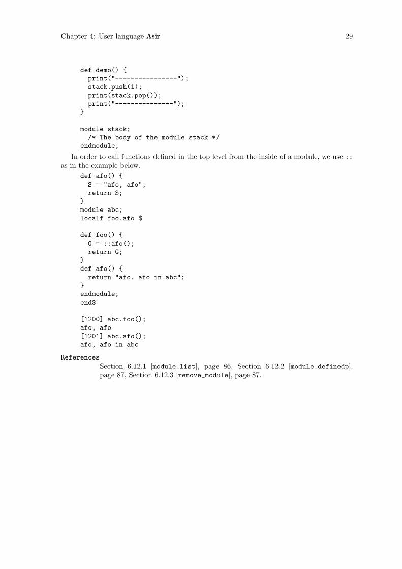
Chapter 4: User language Asir 29
def demo() {print("----------------");stack.push(1);print(stack.pop());print("---------------");
}
module stack;/* The body of the module stack */
endmodule;
In order to call functions defined in the top level from the inside of a module, we use ::as in the example below.
def afo() {S = "afo, afo";return S;
}module abc;localf foo,afo $
def foo() {G = ::afo();return G;
}def afo() {return "afo, afo in abc";
}endmodule;end$
[1200] abc.foo();afo, afo[1201] abc.afo();afo, afo in abc
References
Section 6.12.1 [module_list], page 86, Section 6.12.2 [module_definedp],page 87, Section 6.12.3 [remove_module], page 87.

Chapter 5: Debugger 30
5 Debugger
5.1 What is Debugger
A debugger dbx is available for C programs on Sun, VAX etc. In dbx, one can use commandssuch as setting break-point on a source line, stepwise execution, inspecting a variable’s valueetc. Asir provides such a dbx-like debugger. In addition to such commands, we adoptedseveral useful commands from gdb. In order to enter the debug-mode, type debug; at thetop level of Asir.
[10] debug;(debug)
Asir also enters the debug-mode by the following means or in the following situations.
• When it reaches a break point while executing a program.
• When the ‘d’ option is selected at an interruption.
• When it detects errors while executing a program.
In this case, to continue the execution of the program is impossible. But because itreports the statement in the user defined function that caused the error, then entersthe debug-mode, user can inspect the values of variables at the error state. This helpsto analyze the error and debug the program.
• When built-in function error() is called.
5.2 Debugger commands
Only indispensable commands of dbx are supported in the current version. Generally, theeffect of a command is the same as that of dbx. There are, however, slight differences:Commands step and next execute the next statement, but not the next line; therefore, ifthere are multiple statements in one line, one should issue such commands several times toproceed the next line. The debugger reads in ‘.dbxinit’, which allows the same aliases asis used in dbx.
step Executes the next statement; if the next statement contains a function call,then enters the function.
next Executes the next statement.
finish Enter the debug-mode again after finishing the execuction of the current func-tion. This is useful when an unnecessary step has been executed.
cont
quit Exits from the debug-mode and continues execution.
up [n] Move up the call stack one level. Move up the call stack n levels if n is specified.
down [n] Move down the call stack one level. Move down the call stack n levels if n isspecified.
frame [n] Print the current stack frame with no argument. n specifies the stack framenumber to be selected. Here the stack frame number is a number at the top oflines displayed by executing where.

Chapter 5: Debugger 31
list [startline]list function
Displays ten lines in a source file from startline, the current line if the startlineis not specified, or from the top line of current target function.
print exprDisplays expr.
func functionSet the target function to function.
stop at sourceline [if cond]stop in function
Set a break-point at the sourceline-th line of the source file, or at the top of thetarget function. Break-points are removed whenever the relevant function isredefined. When if statements are repeatedly encountered, Asir enters debug-mode only when the corresponding cond parts are evaluated to a non-zero value.
trace expr at sourceline [if cond]
trace expr in functionThese are similar to stop. trace simply displays the value of expr and withoutentering the debug-mode.
delete n Remove the break point specified by a number n, which can be known by thestatus command.
status Displays a list of the break-points.
where Displays the calling sequence of functions from the top level through the currentlevel.
alias alias commandCreate an alias alias for command
The debugger command print can take almost all expressions as its argument. The ordinaryusage is to print the values of (programming) variables. However, the following usage isworth to remember.
• overwriting the variable
One might sometimes wish to continue the execution with several values of variablesmodified. For such an purpose, take the following procedure.
(debug) print AA = 2(debug) print A=1A=1 = 1(debug) print AA = 1
• function call
A function call is also an expression, therefore, it can appear at the argument place ofprint.
(debug) print length(List)length(List) = 14

Chapter 5: Debugger 32
In this example, the length of the list assigned to the variable List is examined by afunction length().
(debug) print ctrl("cputime",1)ctrl("cputime",1) = 1
This example shows such a usage where measuring CPU time is activated from withinthe debug-mode, even if one might have forgotten to specify the activation of CPUtime measurement.
It is also useful to save intermediate results to files from within the debug-mode by thebuilt-in function bsave() when one is forced to quit the computation by any reason.
(debug) print bsave(A,"savefile")bsave(A,"savefile") = 1
Note that continuation of the parent function will be impossible if an error will occurin the function call from within the debug-mode.
5.3 Execution example of debugger
Here, the usage of the Debugger is explained by showing an example for debugging aprogram which computes the integer factorial by a recursive definition.
% asir[0] load("fac")$[3] debug$(debug) list factorial1 def factorial(X) {2 if ( !X )3 return 1;4 else5 return X * factorial(X - 1);6 }7 end$(debug) stop at 5 <-- setting a break point(0) stop at "./fac":5(debug) quit <-- leaving the debug-mode[4] factorial(6); <-- call for factorial(6)stopped in factorial at line 5 in file "./fac"5 return X * factorial(X - 1);(debug) where <-- display the calling sequencefactorial(), line 5 in "./fac" up to this break point(debug) print X <-- Display the value of XX = 6(debug) step <-- step execution
(enters function)stopped in factorial at line 2 in file "./fac"2 if ( !X )(debug) wherefactorial(), line 2 in "./fac"factorial(), line 5 in "./fac"(debug) print X

Chapter 5: Debugger 33
X = 5(debug) delete 0 <-- delete the break point 0(debug) cont <-- continue execution720 <-- result = 6![5] quit;
5.4 Sample file of initialization file for Debugger
As is previously mentioned, Asir reads in the file ‘$HOME/.dbxinit’ at its invocation. Thisfile is originally used to define various initializing commands for dbx debugger, but Asirrecognizes only alias lines. For example, by the setting
% cat ~/.dbxinitalias n nextalias c contalias p printalias s stepalias d deletealias r runalias l listalias q quit
one can use short aliases, e.g., p, c etc., for frequently used commands such as print, contetc. One can create new aliases in the debug-mode during an execution.
lex_hensel(La,[a,b,c],0,[a,b,c],0);stopped in gennf at line 226 in file "/home/usr3/noro/asir/gr"226 N = length(V); Len = length(G); dp_ord(O); PS = newvect(Len);(debug) p VV = [a,b,c](debug) c...

Chapter 6: Built-in Function 34
6 Built-in Function
6.1 Numbers
6.1.1 idiv, irem
idiv(i1,i2):: Integer quotient of i1 divided by i2.
irem(i1,i2):: Integer remainder of i1 divided by i2.
return integer
i1 i2 integer
• Integer quotient and remainder of i1 divided by i2.
• i2 must not be 0.
• If the dividend is negative, the results are obtained by changing the sign of the resultsfor absolute values of the dividend.
• One can use i1 % i2 for replacement of irem() which only differs in the point that theresult is always normalized to non-negative values.
• Use sdiv(), srem() for polynomial quotient.
[0] idiv(100,7);14[0] idiv(-100,7);-14[1] irem(100,7);2[1] irem(-100,7);-2
References
Section 6.3.8 [sdiv sdivm srem sremm sqr sqrm], page 48, Section 6.3.10 [%],page 50.
6.1.2 fac
fac(i) :: The factorial of i.
return integer
i integer
• The factorial of i.
• Returns 0 if the argument i is negative.
[0] fac(50);30414093201713378043612608166064768844377641568960512000000000000

Chapter 6: Built-in Function 35
6.1.3 igcd,igcdcntl
igcd(i1,i2):: The integer greatest common divisor of i1 and i2.
igcdcntl([i]):: Selects an algorithm for integer GCD.
return integer
i1 i2 i integer
• Function igcd() returns the integer greatest common divisor of the given two integers.
• An error will result if the argument is not an integer; the result is not valid even if oneis returned.
• Use gcd(), gcdz() for polynomial GCD.
• Various method of integer GCD computation are implemented and they can be selectedby igcdcntl.
0 Euclid algorithm (default)
1 binary GCD
2 bmod GCD
3 accelerated integer GCD
2, 3 are due to [Weber].
In most cases 3 is the fastest, but there are exceptions.
[0] A=lrandom(10^4)$[1] B=lrandom(10^4)$[2] C=lrandom(10^4)$[3] D=A*C$[4] E=A*B$[5] cputime(1)$[6] igcd(D,E)$0.6sec + gc : 1.93sec(2.531sec)[7] igcdcntl(1)$[8] igcd(D,E)$0.27sec(0.2635sec)[9] igcdcntl(2)$[10] igcd(D,E)$0.19sec(0.1928sec)[11] igcdcntl(3)$[12] igcd(D,E)$0.08sec(0.08023sec)
References
Section 6.3.20 [gcd gcdz], page 56.

Chapter 6: Built-in Function 36
6.1.4 ilcm
ilcm(i1,i2):: The integer least common multiple of i1 and i2.
return integer
i1 i2 integer
• This function computes the integer least common multiple of i1, i2.
• If one of argument is equal to 0, the return 0.
References
Section 6.1.3 [igcd igcdcntl], page 35, Section 6.1.10 [mt_save mt_load],page 38.
6.1.5 isqrt
isqrt(n) :: The integer square root of n.
return non-negative integer
n non-negative integer
6.1.6 inv
inv(i,m) :: the inverse (reciprocal) of i modulo m.
return integer
i m integer
• This function computes an integer such that ia ≡ 1 mod (m).
• The integer i and m must be mutually prime. However, inv() does not check it.
[71] igcd(1234,4321);1[72] inv(1234,4321);3239[73] irem(3239*1234,4321);1
References
Section 6.1.3 [igcd igcdcntl], page 35.
6.1.7 prime, lprime
prime(index)
lprime(index):: Returns a prime number.
return integer
index integer

Chapter 6: Built-in Function 37
• The two functions, prime() and lprime(), returns an element stored in the systemtable of prime numbers. Here, index is a non-negative integer and be used as an indexfor the prime tables. The function prime() can return one of 1900 primes up to 16381indexed so that the smaller one has smaller index. The function lprime() can returnone of 999 primes which are 8 digit sized and indexed so that the larger one has thesmaller index. The two function always returns 0 for other indices.
• For more general function for prime generation, there is a PARI function
pari(nextprime,number).
[95] prime(0);2[96] prime(1228);9973[97] lprime(0);99999989[98] lprime(999);0
References
Section 6.1.14 [pari], page 40.
6.1.8 random
random([seed])
seedreturn non-negative integer
• Generates a random number which is a non-negative integer less than 2^32.
• If a non zero argument is specified, then after setting it as a random seed, a randomnumber is generated.
• As the default seed is fixed, the sequence of the random numbers is always the same ifa seed is not set.
• The algorithm is Mersenne Twister (http://www.math.keio.ac.jp/matsumoto/mt.html)by M. Matsumoto and T. Nishimura. The implementation is done also by themselves.
• The period of the random number sequence is 2^19937-1.
• One can save the state of the random number generator with mt_save. By loading thestate file with mt_load, one can trace a single random number sequence arcoss multiplesessions.
References
Section 6.1.9 [lrandom], page 37, Section 6.1.10 [mt_save mt_load], page 38.
6.1.9 lrandom
lrandom(bit):: Generates a long random number.
bit

Chapter 6: Built-in Function 38
return integer
• Generates a non-negative integer of at most bit bits.
• The result is a concatination of outputs of random.
References
Section 6.1.8 [random], page 37, Section 6.1.10 [mt_save mt_load], page 38.
6.1.10 mt_save, mt_load
mt_save(fname):: Saves the state of the random number generator.
mt_load(fname):: Loads a saved state of the random number generator.
return 0 or 1
fname string
• One can save the state of the random number generator with mt_save. By loading thestate file with mt_load, one can trace a single random number sequence arcoss multipleAsir sessions.
[340] random();3510405877[341] mt_save("/tmp/mt_state");1[342] random();4290933890[343] quit;% asirThis is Asir, Version 991108.Copyright (C) FUJITSU LABORATORIES LIMITED.3 March 1994. All rights reserved.[340] mt_load("/tmp/mt_state");1[341] random();4290933890
References
Section 6.1.8 [random], page 37, Section 6.1.9 [lrandom], page 37.
6.1.11 nm, dn
nm(rat) :: Numerator of rat.
dn(rat) :: Denominator of rat.
return integer or polynomial
rat rational number or rational expression
• Numerator and denominator of a given rational expression.

Chapter 6: Built-in Function 39
• For a rational number, they return its numerator and denominator, respectively. For arational expression whose numerator and denominator may contain rational numbers,they do not separate those rational coefficients to numerators and denominators.
• For a rational number, the denominator is always kept positive, and the sign is con-tained in the numerator.
• Risa/Asir does not cancel the common divisors unless otherwise explicitly specified bythe user. Therefore, nm() and dn() return the numerator and the denominator as itis, respectively.
[2] [nm(-43/8),dn(-43/8)];[-43,8][3] dn((x*z)/(x*y));y*x[3] dn(red((x*z)/(x*y)));y
References
Section 6.3.21 [red], page 57.
6.1.12 conj, real, imag
real(comp):: Real part of comp.
imag(comp):: Imaginary part of comp.
conj(comp):: Complex conjugate of comp.
return compcomplex number
• Basic operations for complex numbers.
• These functions works also for polynomials with complex coefficients.
[111] A=(2+@i)^3;(2+11*@i)[112] [real(A),imag(A),conj(A)];[2,11,(2-11*@i)]
6.1.13 eval, deval
eval(obj[,prec])
deval(obj):: Evaluate obj numerically.
return number or expression
obj general expression
prec integer
• Evaluates the value of the functions contained in obj as far as possible.

Chapter 6: Built-in Function 40
• deval returns double float. Rational numbers remain unchanged in results from eval.
• In eval the computation is done by PARI. (See Section 6.1.14 [pari], page 40.) Indeval the computation is done by the C math library.
• deval cannot handle complex numbers.
• When prec is specified, computation will be performed with a precision of about prec-digits. If prec is not specified, computation is performed with the precision set currently.(See Section 6.1.15 [setprec], page 41.)
• Currently available numerical functions are listed below. Note they are only a smallpart of whole PARI functions.
sin, cos, tan,
asin, acos, atan,
sinh, cosh, tanh, asinh, acosh, atanh,
exp, log, pow(a,b) (a^b)
• Symbols for special values are as the followings. Note that @i cannot be handled bydeval.
@i unit of imaginary number
@pi the number pi, the ratio of circumference to diameter
@e Napier’s number (exp(1))
[118] eval(exp(@pi*@i));-1.0000000000000000000000000000[119] eval(2^(1/2));1.414213562373095048763788073031[120] eval(sin(@pi/3));0.86602540378443864674620506632[121] eval(sin(@pi/3)-3^(1/2)/2,50);-2.78791084448179148471 E-58[122] eval(1/2);1/2[123] deval(sin(1)^2+cos(1)^2);1
References
Section 6.14.1 [ctrl], page 89, Section 6.1.15 [setprec], page 41, Section 6.1.14[pari], page 40.
6.1.14 pari
pari(func,arg,prec):: Call PARI function func.
return Depends on func.
func Function name of PARI.
arg Arguments of func.
prec integer

Chapter 6: Built-in Function 41
• This command connects Asir to PARI system so that several functions of PARI canbe conveniently used from Risa/Asir.
• PARI [Batut et al.] is developed at Bordeaux University, and distributed as a freesoftware. Though it has a certain facility to computer algebra, its major target is theoperation of numbers (bignum, bigfloat) related to the number theory. It facilitatesvarious function evaluations as well as arithmetic operations at a remarkable speed.It can also be used from other external programs as a library. It provides a languageinterface named ‘gp’ to its library, which enables a user to use PARI as a calculatorwhich runs on UNIX. The current version is 2.0.17beta. It can be obtained by severalftp sites. (For example, ftp://megrez.ceremab.u-bordeaux.fr/pub/pari.)
• The last argument (optional) int specifies the precision in digits for bigfloat operation.If the precision is not explicitly specified, operation will be performed with the precisionset by setprec().
• Currently available functions of PARI system are as follows. Note these are only apart of functions in PARI system. For details of individual functions, refer to thePARI manual. (Some of them can be seen in the following example.)
abs, adj, arg, bigomega, binary, ceil, centerlift, cf, classno, classno2,conj, content, denom, det, det2, detr, dilog, disc, discf, divisors,eigen, eintg1, erfc, eta, floor, frac, galois, galoisconj, gamh, gamma,hclassno, hermite, hess, imag, image, image2, indexrank, indsort, initalg,isfund, isprime, ispsp, isqrt, issqfree, issquare, jacobi, jell, ker,keri, kerint, kerintg1, kerint2, kerr, length, lexsort, lift, lindep, lll,lllg1, lllgen, lllgram, lllgramg1, lllgramgen, lllgramint, lllgramkerim,lllgramkerimgen, lllint, lllkerim, lllkerimgen, lllrat, lngamma, logagm, mat,matrixqz2, matrixqz3, matsize, modreverse, mu, nextprime, norm, norml2, numdiv,numer, omega, order, ordred, phi, pnqn, polred, polred2, primroot, psi, quadgen,quadpoly, real, recip, redcomp, redreal, regula, reorder, reverse, rhoreal,roots, rootslong, round, sigma, signat, simplify, smalldiscf, smallfact,smallpolred, smallpolred2, smith, smith2, sort, sqr, sqred, sqrt, supplement,trace, trans, trunc, type, unit, vec, wf, wf2, zeta
• Asir currently uses only a very small subset of PARI. We will improve Asir so that itcan provide more functions of PARI.
/* Eigen vectors of a numerical matrix */[0] pari(eigen,newmat(2,2,[[1,1],[1,2]]));[ -1.61803398874989484819771921990 0.61803398874989484826 ][ 1 1 ]/* Roots of a polynomial */[1] pari(roots,t^2-2);[ -1.41421356237309504876 1.41421356237309504876 ]
References
Section 6.1.15 [setprec], page 41.
6.1.15 setprec
setprec([n]):: Sets the precision for bigfloat operations to n digits.

Chapter 6: Built-in Function 42
return integer
n integer
• When an argument is given, it sets the precision for bigfloat operations to n digits. Thereturn value is always the previous precision in digits regardless of the existence of anargument.
• Bigfloat operations are done by PARI. (See Section 6.1.14 [pari], page 40.)
• This is effective for computations in bigfloat. Refer to ctrl() for turning on the‘bigfloat flag.’
• There is no upper limit for precision digits. It sets the precision to some digits aroundthe specified precision. Therefore, it is safe to specify a larger value.
[1] setprec();9[2] setprec(100);9[3] setprec(100);96
Section 6.14.1 [ctrl], page 89, Section 6.1.13 [eval deval], page 39,Section 6.1.14 [pari], page 40.
6.1.16 setmod
setmod([p]):: Sets the ground field to GF(p).
return integer
n prime less than 2^27
• Sets the ground field to GF(p) and returns the value p.
• A member of a finite field does not have any information about the field and thearithmetic operations over GF(p) are applied with p set at the time.
• As for large finite fields, see Chapter 10 [Finite fields], page 165.
[0] A=dp_mod(dp_ptod(2*x,[x]),3,[]);(2)*<<1>>[1] A+A;addmi : invalid modulusreturn to toplevel[1] setmod(3);3[2] A+A;(1)*<<1>>
References
Section 8.10.13 [dp_mod dp_rat], page 138, Section 3.2 [Types of numbers],page 13.

Chapter 6: Built-in Function 43
6.1.17 ntoint32, int32ton
ntoint32(n)int32ton(int32)
:: Type-conversion between a non-negative integer and an unsigned 32bit inte-ger.
return unsigned 32bit integer or non-negative integer
n non-negative interger less than 2^32
int32 unsigned 32bit integer
• These functions do conversions between non-negative integers (the type id 1) and un-signed 32bit integers (the type id 10).
• An unsigned 32bit integer is a fundamental construct of OpenXM and one often hasto send an integer to a server as an unsigned 32bit integer. These functions are usedin such a case.
References
Chapter 7 [Distributed computation], page 99, Section 3.2 [Types of
numbers], page 13.
6.2 Bit operations
6.2.1 iand, ior, ixor
iand(i1,i2):: bitwise and
ior(i1,i2):: bitwise or
ixor(i1,i2):: bitwise xor
return integer
i1 i2 integer
• The absolute value of the argument is regarded as a bit string.
• The sign of the argument is ignored and a non-negative integer is returned.
[0] ctrl("hex",1);0x1[1] iand(0xeeeeeeeeeeeeeeee,0x2984723234812312312);0x4622224802202202[2] ior(0xa0a0a0a0a0a0a0a0,0xb0c0b0b0b0b0b0b);0xabacabababababab[3] ixor(0xfffffffffff,0x234234234234);0x2cbdcbdcbdcb
References
Section 6.2.2 [ishift], page 44.

Chapter 6: Built-in Function 44
6.2.2 ishift
ishift(i,count):: bit shift
return integer
i count integer
• The absolute value of i is regarded as a bit string.
• The sign of i is ignored and a non-negative integer is returned.
• If count is positive, then i is shifted to the right. If count is negative, then i is shiftedto the left.
[0] ctrl("hex",1);0x1[1] ishift(0x1000000,12);0x1000[2] ishift(0x1000,-12);0x1000000[3] ixor(0x1248,ishift(1,-16)-1);
References
Section 6.2.1 [iand ior ixor], page 43.
6.3 operations with polynomials and rational expressions
6.3.1 var
var(rat) :: Main variable (indeterminate) of rat.
return indeterminate
rat rational expression
• See Section 3.1 [Types in Asir], page 10 for main variable.
• Indeterminates (variables) are ordered by default as follows.
x, y, z, u, v, w, p, q, r, s, t, a, b, c, d, e, f, g, h, i, j, k, l, m, n, o. The other variableswill be ordered after the above noted variables so that the first comer will be orderedprior to the followers.
[0] var(x^2+y^2+a^2);x[1] var(a*b*c*d*e);a[2] var(3/abc+2*xy/efg);abc
References
Section 6.3.7 [ord], page 47, Section 6.3.2 [vars], page 45.

Chapter 6: Built-in Function 45
6.3.2 vars
vars(obj) :: A list of variables (indeterminates) in an expression obj.
return list
obj arbitrary
• Returns a list of variables (indeterminates) contained in a given expression.
• Lists variables according to the variable ordering.
[0] vars(x^2+y^2+a^2);[x,y,a][1] vars(3/abc+2*xy/efg);[abc,xy,efg][2] vars([x,y,z]);[x,y,z]
References
Section 6.3.1 [var], page 44, Section 6.3.3 [uc], page 45, Section 6.3.7 [ord],page 47.
6.3.3 uc
uc() :: Create a new indeterminate for an undermined coeficient.
return indeterminate with its vtype 1.
• At every evaluation of command uc(), a new indeterminate in the sequence of inde-terminates _0, _1, _2, . . . is created successively.
• Indeterminates created by uc() cannot be input on the keyboard. By this property,you are free, no matter how many indeterminates you will create dynamically by aprogram, from collision of created names with indeterminates input from the keyboardor from program files.
• Functions, rtostr() and strtov(), are used to create ordinary indeterminates (inde-terminates having 0 for their vtype).
• Kernel sub-type of indeterminates created by uc() is 1. (vtype(uc())=1)
[0] A=uc();_0[1] B=uc();_1[2] (uc()+uc())^2;_2^2+2*_3*_2+_3^2[3] (A+B)^2;_0^2+2*_1*_0+_1^2
References
Section 6.8.3 [vtype], page 76, Section 6.10.1 [rtostr], page 77, Section 6.10.2[strtov], page 78.

Chapter 6: Built-in Function 46
6.3.4 coef
coef(poly,deg[,var]):: The coefficient of a polynomial poly at degree deg with respect to the variablevar (main variable if unspecified).
return polynomial
poly polynomial
var indeterminate
deg non-negative integer
• The coefficient of a polynomial poly at degree deg with respect to the variable var.
• The default value for var is the main variable, i.e., var(poly).
• For multi-variate polynomials, access to coefficients depends on the specified indeter-minates. For example, taking coef for the main variable is much faster than for othervariables.
[0] A = (x+y+z)^3;x^3+(3*y+3*z)*x^2+(3*y^2+6*z*y+3*z^2)*x+y^3+3*z*y^2+3*z^2*y+z^3[1] coef(A,1,y);3*x^2+6*z*x+3*z^2[2] coef(A,0);y^3+3*z*y^2+3*z^2*y+z^3
References
Section 6.3.1 [var], page 44, Section 6.3.5 [deg mindeg], page 46.
6.3.5 deg, mindeg
deg(poly,var):: The degree of a polynomial poly with respect to variable.
mindeg(poly,var):: The least exponent of the terms with non-zero coefficients in a polynomialpoly with respect to the variable var. In this manual, this quantity is sometimesreferred to the minimum degree of a polynomial for short.
return non-negative integer
poly polynomial
var indeterminate
• The least exponent of the terms with non-zero coefficients in a polynomial poly withrespect to the variable var. In this manual, this quantity is sometimes referred to theminimum degree of a polynomial for short.
• Variable var must be specified.
[0] deg((x+y+z)^10,x);10[1] deg((x+y+z)^10,w);0[75] mindeg(x^2+3*x*y,x);1

Chapter 6: Built-in Function 47
6.3.6 nmono
nmono(rat):: Number of monomials in rational expression rat.
return non-negative integer
rat rational expression
• Number of monomials with non-zero number coefficients in the full expanded form ofthe given polynomial.
• For a rational expression, the sum of the numbers of monomials of the numerator anddenominator.
• A function form is regarded as a single indeterminate no matter how complex argumentsit has.
[0] nmono((x+y)^10);11[1] nmono((x+y)^10/(x+z)^10);22[2] nmono(sin((x+y)^10));1
References
Section 6.8.3 [vtype], page 76.
6.3.7 ord
ord([varlist]):: It sets the ordering of indeterminates (variables).
return list of indeterminates
varlist list of indeterminates
• When an argument is given, this function rearranges the ordering of variables (inde-terminates) so that the indeterminates in the argument varlist precede and the otherindeterminates follow in the system’s variable ordering. Regardless of the existence ofan argument, it always returns the final variable ordering.
• Note that no change will be made to the variable ordering of internal forms of objectswhich already exists in the system, no matter what reordering you specify. Therefore,the reordering should be limited to the time just after starting Asir, or to the time whenone has decided himself to start a totally new computation which has no relation withthe previous results. Note that unexpected results may be obtained from operationsbetween objects which are created under different variable ordering.
[0] ord();[x,y,z,u,v,w,p,q,r,s,t,a,b,c,d,e,f,g,h,i,j,k,l,m,n,o,_x,_y,_z,_u,_v,_w,_p,_q,_r,_s,_t,_a,_b,_c,_d,_e,_f,_g,_h,_i,_j,_k,_l,_m,_n,_o,exp(_x),(_x)^(_y),log(_x),(_x)^(_y-1),cos(_x),sin(_x),tan(_x),(-_x^2+1)^(-1/2),cosh(_x),sinh(_x),tanh(_x),(_x^2+1)^(-1/2),(_x^2-1)^(-1/2)][1] ord([dx,dy,dz,a,b,c]);

Chapter 6: Built-in Function 48
[dx,dy,dz,a,b,c,x,y,z,u,v,w,p,q,r,s,t,d,e,f,g,h,i,j,k,l,m,n,o,_x,_y,_z,_u,_v,_w,_p,_q,_r,_s,_t,_a,_b,_c,_d,_e,_f,_g,_h,_i,_j,_k,_l,_m,_n,_o,exp(_x),(_x)^(_y),log(_x),(_x)^(_y-1),cos(_x),sin(_x),tan(_x),(-_x^2+1)^(-1/2),cosh(_x),sinh(_x),tanh(_x),(_x^2+1)^(-1/2),(_x^2-1)^(-1/2)]
6.3.8 sdiv, sdivm, srem, sremm, sqr, sqrm
sdiv(poly1,poly2[,v])sdivm(poly1,poly2,mod[,v])
:: Quotient of poly1 divided by poly2 provided that the division can be per-formed within polynomial arithmetic over the rationals.
srem(poly1,poly2[,v])
sremm(poly1,poly2,mod[,v]):: Remainder of poly1 divided by poly2 provided that the division can beperformed within polynomial arithmetic over the rationals.
sqr(poly1,poly2[,v])
sqrm(poly1,poly2,mod[,v]):: Quotient and remainder of poly1 divided by poly2 provided that the divisioncan be performed within polynomial arithmetic over the rationals.
return sdiv(), sdivm(), srem(), sremm() : polynomial sqr(), sqrm() : a list[quotient,remainder]
poly1 poly2polynomial
v indeterminate
mod prime
• Regarding poly1 as an uni-variate polynomial in the main variable of poly2, i.e.var(poly2) (v if specified), sdiv() and srem() compute the polynomial quotient andremainder of poly1 divided by poly2.
• sdivm(), sremm(), sqrm() execute the same operation over GF(mod).
• Division operation of polynomials is performed by the following steps: (1) obtain thequotient of leading coefficients; let it be Q; (2) remove the leading term of poly1 bysubtracting, from poly1, the product of Q with some powers of main variable and poly2;obtain a new poly1; (3) repeat the above step until the degree of poly1 become smallerthan that of poly2. For fulfillment, by operating in polynomials, of this procedure,the divisions at step (1) in every repetition must be an exact division of polynomials.This is the true meaning of what we say “division can be performed within polynomialarithmetic over the rationals.”
• There are typical cases where the division is possible: leading coefficient of poly2 is arational number; poly2 is a factor of poly1.
• Use sqr() to get both the quotient and remainder at once.
• Use idiv(), irem() for integer quotient.
• For remainder operation on all integer coefficients, use %.

Chapter 6: Built-in Function 49
[0] sdiv((x+y+z)^3,x^2+y+a);x+3*y+3*z[1] srem((x+y+z)^2,x^2+y+a);(2*y+2*z)*x+y^2+(2*z-1)*y+z^2-a[2] X=(x+y+z)*(x-y-z)^2;x^3+(-y-z)*x^2+(-y^2-2*z*y-z^2)*x+y^3+3*z*y^2+3*z^2*y+z^3[3] Y=(x+y+z)^2*(x-y-z);x^3+(y+z)*x^2+(-y^2-2*z*y-z^2)*x-y^3-3*z*y^2-3*z^2*y-z^3[4] G=gcd(X,Y);x^2-y^2-2*z*y-z^2[5] sqr(X,G);[x-y-z,0][6] sqr(Y,G);[x+y+z,0][7] sdiv(y*x^3+x+1,y*x+1);divsp: cannot happenreturn to toplevel
References
Section 6.1.1 [idiv irem], page 34, Section 6.3.10 [%], page 50.
6.3.9 tdiv
tdiv(poly1,poly2):: Tests whether poly2 divides poly1.
return Quotient if poly2 divides poly1, 0 otherwise.
poly1 poly2polynomial
• Tests whether poly2 divides poly1 in polynomial ring.
• One application of this function: Consider the case where a polynomial is certainly anirreducible factor of the other polynomial, but the multiplicity of the factor is unknown.Application of tdiv() to the polynomials repeatedly yields the multiplicity.
[11] Y=(x+y+z)^5*(x-y-z)^3;x^8+(2*y+2*z)*x^7+(-2*y^2-4*z*y-2*z^2)*x^6+(-6*y^3-18*z*y^2-18*z^2*y-6*z^3)*x^5+(6*y^5+30*z*y^4+60*z^2*y^3+60*z^3*y^2+30*z^4*y+6*z^5)*x^3+(2*y^6+12*z*y^5+30*z^2*y^4+40*z^3*y^3+30*z^4*y^2+12*z^5*y+2*z^6)*x^2+(-2*y^7-14*z*y^6-42*z^2*y^5-70*z^3*y^4-70*z^4*y^3-42*z^5*y^2-14*z^6*y-2*z^7)*x-y^8-8*z*y^7-28*z^2*y^6-56*z^3*y^5-70*z^4*y^4-56*z^5*y^3-28*z^6*y^2-8*z^7*y-z^8[12] for(I=0,F=x+y+z,T=Y; T=tdiv(T,F); I++);[13] I;5
References
Section 6.3.8 [sdiv sdivm srem sremm sqr sqrm], page 48.

Chapter 6: Built-in Function 50
6.3.10 %
poly % m :: integer remainder to all integer coefficients of the polynomial.
return integer or polynomial
poly integer or polynomial with integer coefficients
m intger
• Returns a polynomial whose coefficients are remainders of the coefficients of the inputpolynomial divided by m.
• The resulting coefficients are all normalized to non-negative integers.
• An integer is allowed for poly. This can be used for an alternative for irem() exceptthat the result is normalized to a non-negative integer.
• Coefficients of poly and m must all be integers, though the type checking is not done.
[0] (x+2)^5 % 3;x^5+x^4+x^3+2*x^2+2*x+2[1] (x-2)^5 % 3;x^5+2*x^4+x^3+x^2+2*x+1[2] (-5) % 4;3[3] irem(-5,4);-1
References
Section 6.1.1 [idiv irem], page 34.
6.3.11 subst, psubst
subst(rat[,varn,ratn]*)
psubst(rat[,var,rat]*):: Substitute ratn for varn in expression rat. (n=1,2,. . . . Substitution will bedone successively from left to right if arguments are repeated.)
return rational expression
rat ratn rational expression
varn indeterminate
• Substitutes rational expressions for specified kernels in a rational expression.
• subst(r,v1,r1,v2,r2,. . . ) has the same effect as subst(subst(r,v1,r1),v2,r2,. . . ).
• Note that repeated substitution is done from left to right successively. You may getdifferent result by changing the specification order.
• Ordinary subst() performs substitution at all levels of a scalar algebraic expressioncreeping into arguments of function forms recursively. Function psubst() regardssuch a function form as an independent indeterminate, and does not attempt to applysubstitution to its arguments. (The name comes after Partial SUBSTitution.)
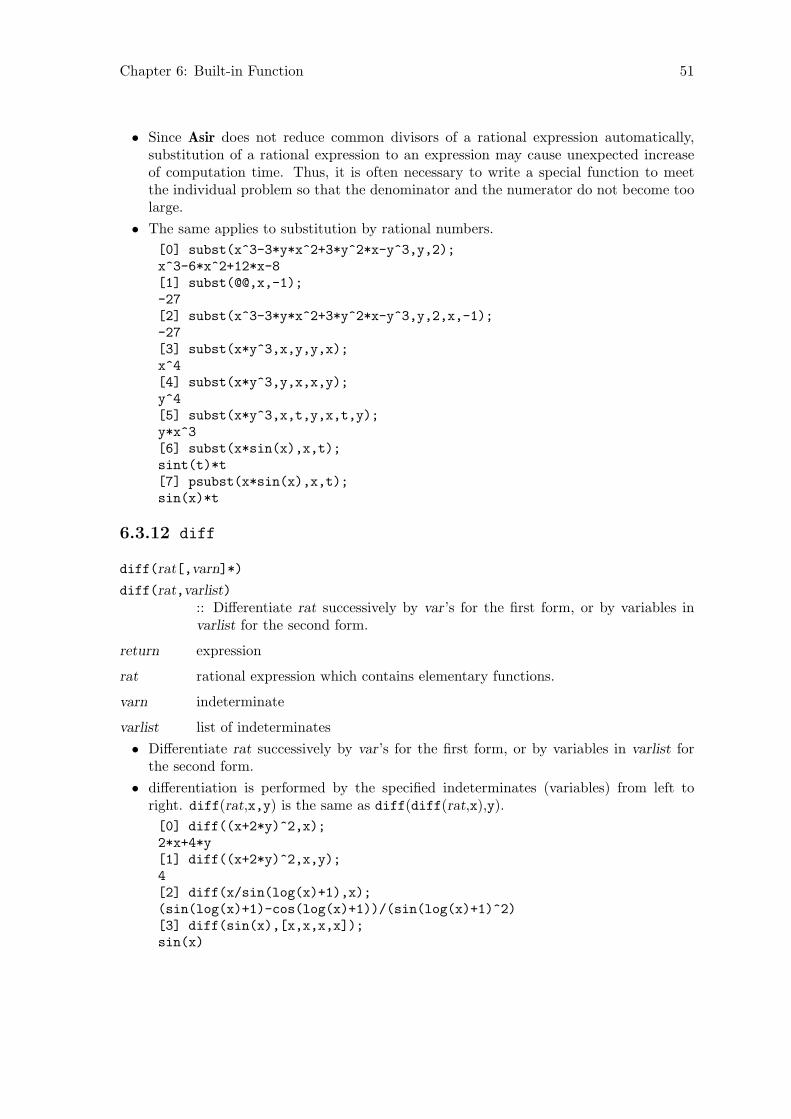
Chapter 6: Built-in Function 51
• Since Asir does not reduce common divisors of a rational expression automatically,substitution of a rational expression to an expression may cause unexpected increaseof computation time. Thus, it is often necessary to write a special function to meetthe individual problem so that the denominator and the numerator do not become toolarge.
• The same applies to substitution by rational numbers.
[0] subst(x^3-3*y*x^2+3*y^2*x-y^3,y,2);x^3-6*x^2+12*x-8[1] subst(@@,x,-1);-27[2] subst(x^3-3*y*x^2+3*y^2*x-y^3,y,2,x,-1);-27[3] subst(x*y^3,x,y,y,x);x^4[4] subst(x*y^3,y,x,x,y);y^4[5] subst(x*y^3,x,t,y,x,t,y);y*x^3[6] subst(x*sin(x),x,t);sint(t)*t[7] psubst(x*sin(x),x,t);sin(x)*t
6.3.12 diff
diff(rat[,varn]*)
diff(rat,varlist):: Differentiate rat successively by var’s for the first form, or by variables invarlist for the second form.
return expression
rat rational expression which contains elementary functions.
varn indeterminate
varlist list of indeterminates
• Differentiate rat successively by var’s for the first form, or by variables in varlist forthe second form.
• differentiation is performed by the specified indeterminates (variables) from left toright. diff(rat,x,y) is the same as diff(diff(rat,x),y).
[0] diff((x+2*y)^2,x);2*x+4*y[1] diff((x+2*y)^2,x,y);4[2] diff(x/sin(log(x)+1),x);(sin(log(x)+1)-cos(log(x)+1))/(sin(log(x)+1)^2)[3] diff(sin(x),[x,x,x,x]);sin(x)

Chapter 6: Built-in Function 52
6.3.13 ediff
ediff(poly[,varn]*)
ediff(poly,varlist):: Differentiate poly successively by Euler operators of var’s for the first form,or by Euler operators of variables in varlist for the second form.
return polynomial
poly polynomial
varn indeterminate
varlist list of indeterminates
• differentiation is performed by the specified indeterminates (variables) from left toright. ediff(poly,x,y) is the same as ediff(ediff(poly,x),y).
[0] ediff((x+2*y)^2,x);2*x^2+4*y*x[1] ediff((x+2*y)^2,x,y);4*y*x
6.3.14 res
res(var,poly1,poly2[,mod]):: Resultant of poly1 and poly2 with respect to var.
return polynomial
var indeterminate
poly1 poly2polynomial
mod prime
• Resultant of two polynomials poly1 and poly2 with respect to var.
• Sub-resultant algorithm is used to compute the resultant.
• The computation is done over GF(mod) if mod is specified.
[0] res(t,(t^3+1)*x+1,(t^3+1)*y+t);-x^3-x^2-y^3
6.3.15 fctr, sqfr
fctr(poly):: Factorize polynomial poly over the rationals.
sqfr(poly):: Gets a square-free factorization of polynomial poly.
return list
poly polynomial with rational coefficients

Chapter 6: Built-in Function 53
• Factorizes polynomial poly over the rationals. fctr() for irreducible factorization;sqfr() for square-free factorization.
• The result is represented by a list, whose elements are a pair represented as
[[num,1],[factor,multiplicity],...].
• Products of all factor^multiplicity and num is equal to poly.
• The number num is determined so that (poly/num) is an integral polynomial and itscontent (GCD of all coefficients) is 1. (See Section 6.3.18 [ptozp], page 55.)
[0] fctr(x^10-1);[[1,1],[x-1,1],[x+1,1],[x^4+x^3+x^2+x+1,1],[x^4-x^3+x^2-x+1,1]][1] fctr(x^3+y^3+(z/3)^3-x*y*z);[[1/27,1],[9*x^2+(-9*y-3*z)*x+9*y^2-3*z*y+z^2,1],[3*x+3*y+z,1]][2] A=(a+b+c+d)^2;a^2+(2*b+2*c+2*d)*a+b^2+(2*c+2*d)*b+c^2+2*d*c+d^2[3] fctr(A);[[1,1],[a+b+c+d,2]][4] A=(x+1)*(x^2-y^2)^2;x^5+x^4-2*y^2*x^3-2*y^2*x^2+y^4*x+y^4[5] sqfr(A);[[1,1],[x+1,1],[-x^2+y^2,2]][6] fctr(A);[[1,1],[x+1,1],[-x-y,2],[x-y,2]]
References
Section 6.3.16 [ufctrhint], page 53.
6.3.16 ufctrhint
ufctrhint(poly,hint):: Factorizes uni-variate polynomial poly over the rational number field whenthe degrees of its factors are known to be some integer multiples of hint.
return list
poly uni-variate polynomial with rational coefficients
hint non-negative integer
• By any reason, if the degree of all the irreducible factors of poly is known to be somemultiples of hint, factors can be computed more efficiently by the knowledge thanfctr().
• When hint is 1, ufctrhint() is the same as fctr() for uni-variate polynomials. Antypical application where ufctrhint() is effective: Consider the case where poly isa norm (Chapter 9 [Algebraic numbers], page 152) of a certain polynomial over anextension field with its extension degree d, and it is square free; Then, every irreduciblefactor has a degree that is a multiple of d.
[10] A=t^9-15*t^6-87*t^3-125;t^9-15*t^6-87*t^3-1250msec[11] N=res(t,subst(A,t,x-2*t),A);

Chapter 6: Built-in Function 54
-x^81+1215*x^78-567405*x^75+139519665*x^72-19360343142*x^69+1720634125410*x^66-88249977024390*x^63-4856095669551930*x^60+1999385245240571421*x^57-15579689952590251515*x^54+15956967531741971462865*x^51...+140395588720353973535526123612661444550659875*x^6+10122324287343155430042768923500799484375*x^3+139262743444407310133459021182733314453125980msec + gc : 250msec[12] sqfr(N);[[-1,1],[x^81-1215*x^78+567405*x^75-139519665*x^72+19360343142*x^69-1720634125410*x^66+88249977024390*x^63+4856095669551930*x^60-1999385245240571421*x^57+15579689952590251515*x^54...-10122324287343155430042768923500799484375*x^3-139262743444407310133459021182733314453125,1]]20msec[13] fctr(N);[[-1,1],[x^9-405*x^6-63423*x^3-2460375,1],[x^18-486*x^15+98739*x^12-9316620*x^9+945468531*x^6-12368049246*x^3+296607516309,1],[x^18-8667*x^12+19842651*x^6+19683,1],[x^18-324*x^15+44469*x^12-1180980*x^9+427455711*x^6+2793253896*x^3+31524548679,1],[x^18+10773*x^12+2784051*x^6+307546875,1]]167.050sec + gc : 1.890sec[14] ufctrhint(N,9);[[-1,1],[x^9-405*x^6-63423*x^3-2460375,1],[x^18-486*x^15+98739*x^12-9316620*x^9+945468531*x^6-12368049246*x^3+296607516309,1],[x^18-8667*x^12+19842651*x^6+19683,1],[x^18-324*x^15+44469*x^12-1180980*x^9+427455711*x^6+2793253896*x^3+31524548679,1],[x^18+10773*x^12+2784051*x^6+307546875,1]]119.340sec + gc : 1.300sec
References
Section 6.3.15 [fctr sqfr], page 52.
6.3.17 modfctr
modfctr(poly,mod):: Factorizer over small finite fields
return list
poly Polynomial with integer coefficients
mod non-negative integer
• This function factorizes a polynomial poly over the finite prime field of characteristicmod, where mod must be smaller than 2^29.
• The result is represented by a list, whose elements are a pair represented as
[[num,1],[factor,multiplicity],...].
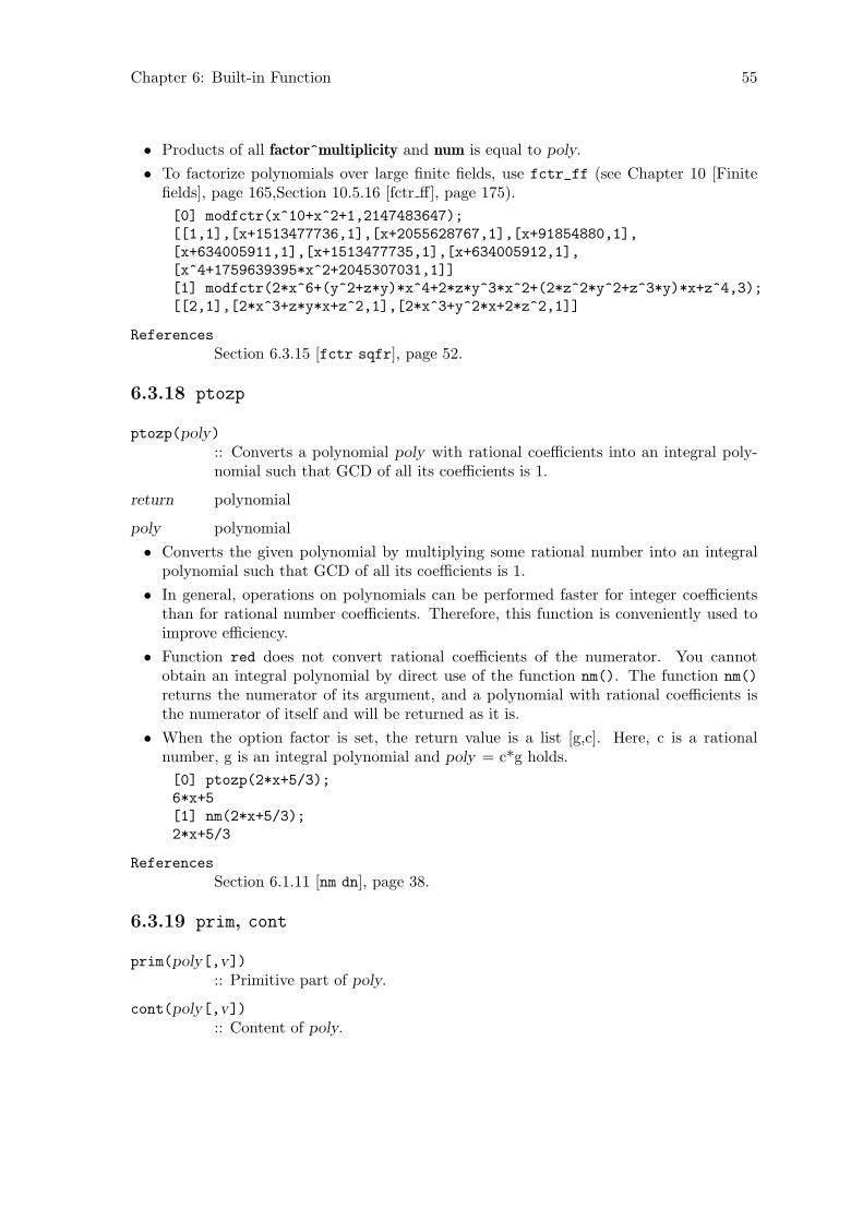
Chapter 6: Built-in Function 55
• Products of all factor^multiplicity and num is equal to poly.
• To factorize polynomials over large finite fields, use fctr_ff (see Chapter 10 [Finitefields], page 165,Section 10.5.16 [fctr ff], page 175).
[0] modfctr(x^10+x^2+1,2147483647);[[1,1],[x+1513477736,1],[x+2055628767,1],[x+91854880,1],[x+634005911,1],[x+1513477735,1],[x+634005912,1],[x^4+1759639395*x^2+2045307031,1]][1] modfctr(2*x^6+(y^2+z*y)*x^4+2*z*y^3*x^2+(2*z^2*y^2+z^3*y)*x+z^4,3);[[2,1],[2*x^3+z*y*x+z^2,1],[2*x^3+y^2*x+2*z^2,1]]
References
Section 6.3.15 [fctr sqfr], page 52.
6.3.18 ptozp
ptozp(poly):: Converts a polynomial poly with rational coefficients into an integral poly-nomial such that GCD of all its coefficients is 1.
return polynomial
poly polynomial
• Converts the given polynomial by multiplying some rational number into an integralpolynomial such that GCD of all its coefficients is 1.
• In general, operations on polynomials can be performed faster for integer coefficientsthan for rational number coefficients. Therefore, this function is conveniently used toimprove efficiency.
• Function red does not convert rational coefficients of the numerator. You cannotobtain an integral polynomial by direct use of the function nm(). The function nm()
returns the numerator of its argument, and a polynomial with rational coefficients isthe numerator of itself and will be returned as it is.
• When the option factor is set, the return value is a list [g,c]. Here, c is a rationalnumber, g is an integral polynomial and poly = c*g holds.
[0] ptozp(2*x+5/3);6*x+5[1] nm(2*x+5/3);2*x+5/3
References
Section 6.1.11 [nm dn], page 38.
6.3.19 prim, cont
prim(poly[,v]):: Primitive part of poly.
cont(poly[,v]):: Content of poly.

Chapter 6: Built-in Function 56
return polypolynomial over the rationals
v indeterminate
• The primitive part and the content of a polynomial poly with respect to its mainvariable (v if specified).
[0] E=(y-z)*(x+y)*(x-z)*(2*x-y);(2*y-2*z)*x^3+(y^2-3*z*y+2*z^2)*x^2+(-y^3+z^2*y)*x+z*y^3-z^2*y^2[1] prim(E);2*x^3+(y-2*z)*x^2+(-y^2-z*y)*x+z*y^2[2] cont(E);y-z[3] prim(E,z);(y-z)*x-z*y+z^2
References
Section 6.3.1 [var], page 44, Section 6.3.7 [ord], page 47.
6.3.20 gcd, gcdz
gcd(poly1,poly2[,mod])
gcdz(poly1,poly2):: The polynomial greatest common divisor of poly1 and poly2.
return polynomial
poly1 poly2polynomial
mod prime
• Functions gcd() and gcdz() return the greatest common divisor (GCD) of the giventwo polynomials.
• Function gcd() returns an integral polynomial GCD over the rational number field.The coefficients are normalized such that their GCD is 1. It returns 1 in case that thegiven polynomials are mutually prime.
• Function gcdz() works for arguments of integral polynomials, and returns a polynomialGCD over the integer ring, that is, it returns gcd() multiplied by the contents of allcoefficients of the two input polynomials.
• gcd() computes the GCD over GF(mod) if mod is specified.
• Polynomial GCD is computed by an improved algorithm based on Extended Zassenhausalgorithm.
• GCD over a finite field is computed by PRS algorithm and it may not be efficient forlarge inputs and co-prime inputs.
[0] gcd(12*(x^2+2*x+1)^2,18*(x^2+(y+1)*x+y)^3);x^3+3*x^2+3*x+1[1] gcdz(12*(x^2+2*x+1)^2,18*(x^2+(y+1)*x+y)^3);6*x^3+18*x^2+18*x+6[2] gcd((x+y)*(x-y)^2,(x+y)^2*(x-y));
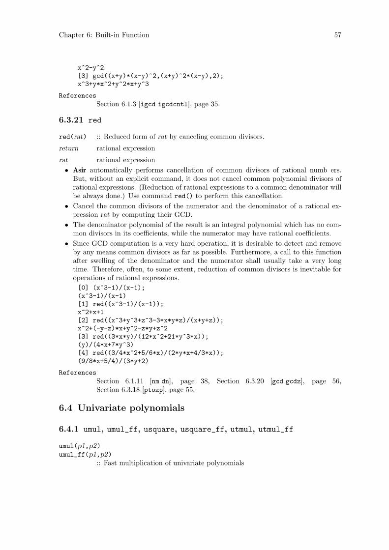
Chapter 6: Built-in Function 57
x^2-y^2[3] gcd((x+y)*(x-y)^2,(x+y)^2*(x-y),2);x^3+y*x^2+y^2*x+y^3
References
Section 6.1.3 [igcd igcdcntl], page 35.
6.3.21 red
red(rat) :: Reduced form of rat by canceling common divisors.
return rational expression
rat rational expression
• Asir automatically performs cancellation of common divisors of rational numb ers.But, without an explicit command, it does not cancel common polynomial divisors ofrational expressions. (Reduction of rational expressions to a common denominator willbe always done.) Use command red() to perform this cancellation.
• Cancel the common divisors of the numerator and the denominator of a rational ex-pression rat by computing their GCD.
• The denominator polynomial of the result is an integral polynomial which has no com-mon divisors in its coefficients, while the numerator may have rational coefficients.
• Since GCD computation is a very hard operation, it is desirable to detect and removeby any means common divisors as far as possible. Furthermore, a call to this functionafter swelling of the denominator and the numerator shall usually take a very longtime. Therefore, often, to some extent, reduction of common divisors is inevitable foroperations of rational expressions.
[0] (x^3-1)/(x-1);(x^3-1)/(x-1)[1] red((x^3-1)/(x-1));x^2+x+1[2] red((x^3+y^3+z^3-3*x*y*z)/(x+y+z));x^2+(-y-z)*x+y^2-z*y+z^2[3] red((3*x*y)/(12*x^2+21*y^3*x));(y)/(4*x+7*y^3)[4] red((3/4*x^2+5/6*x)/(2*y*x+4/3*x));(9/8*x+5/4)/(3*y+2)
References
Section 6.1.11 [nm dn], page 38, Section 6.3.20 [gcd gcdz], page 56,Section 6.3.18 [ptozp], page 55.
6.4 Univariate polynomials
6.4.1 umul, umul_ff, usquare, usquare_ff, utmul, utmul_ff
umul(p1,p2)umul_ff(p1,p2)
:: Fast multiplication of univariate polynomials

Chapter 6: Built-in Function 58
usquare(p1)usquare_ff(p1)
:: Fast squaring of a univariate polynomial
utmul(p1,p2,d)utmul_ff(p1,p2,d)
:: Fast multiplication of univariate polynomials with truncation
return univariate polynomial
p1 p2 univariate polynomial
d non-negative integer
• These functions compute products of univariate polynomials by selecting an appropriatealgorithm depending on the degrees of inputs.
• umul(), usquare(), utmul() compute products over the integers. Coefficients in GF(p)are regarded as non-negative integers less than p.
• umul_ff(), usquare_ff(), utmul_ff() compute products over a finite field. However,if some of the coefficients of the inputs are integral, the result may be an integralpolynomial. So if one wants to assure that the result is a polynomial over the finitefield, apply simp_ff() to the inputs.
• umul_ff(), usquare_ff(), utmul_ff() cannot take polynomials over GF(2^n) as theirinputs.
• umul(), umul_ff() produce p1*p2. usquare(), usquare_ff() produce p1^2.utmul(), utmul_ff() produce p1*p2 mod v^(d+1), where v is the variable of p1, p2.
• If the degrees of the inputs are less than or equal to the value returned by set_upkara()(set_uptkara() for utmul, utmul_ff), usual pencil and paper method is used. If thedegrees of the inputs are less than or equall to the value returned by set_upfft(),Karatsuba algorithm is used. If the degrees of the inputs exceed it, a combination ofFFT and Chinese remainder theorem is used. First of all sufficiently many primes miwithin 1 machine word are prepared. Then p1*p2 mod mi is computed by FFT foreach mi. Finally they are combined by Chinese remainder theorem. The functions overfinite fields use an improvement by V. Shoup [Shoup].
[176] load("fff")$[177] cputime(1)$0sec(1.407e-05sec)[178] setmod_ff(2^160-47);14615016373309029182036848327162830196559325429290sec(0.00028sec)[179] A=randpoly_ff(100,x)$0sec(0.001422sec)[180] B=randpoly_ff(100,x)$0sec(0.00107sec)[181] for(I=0;I<100;I++)A*B;7.77sec + gc : 8.38sec(16.15sec)[182] for(I=0;I<100;I++)umul(A,B);2.24sec + gc : 1.52sec(3.767sec)[183] for(I=0;I<100;I++)umul_ff(A,B);

Chapter 6: Built-in Function 59
1.42sec + gc : 0.24sec(1.653sec)[184] for(I=0;I<100;I++)usquare_ff(A);1.08sec + gc : 0.21sec(1.297sec)[185] for(I=0;I<100;I++)utmul_ff(A,B,100);1.2sec + gc : 0.17sec(1.366sec)[186] deg(utmul_ff(A,B,100),x);100
References
Section 6.4.3 [set_upkara set_uptkara set_upfft], page 59, Section 6.4.2[kmul ksquare ktmul], page 59.
6.4.2 kmul, ksquare, ktmul
kmul(p1,p2):: Fast multiplication of univariate polynomials
ksquare(p1):: Fast squaring of a univariate polynomial
ktmul(p1,p2,d):: Fast multiplication of univariate polynomials with truncation
return univariate polynomial
p1 p2 univariate polynomial
d non-negative integer
These functions compute products of univariate polynomials by Karatsuba algorithm.
• These functions do not apply FFT for large degree inputs.
• These functions can compute products over GF(2^n).
[0] load("code/fff");1[34] setmod_ff(defpoly_mod2(160));x^160+x^5+x^3+x^2+1[35] A=randpoly_ff(100,x)$[36] B=randpoly_ff(100,x)$[37] umul(A,B)$umul : invalid argumentreturn to toplevel[37] kmul(A,B)$
6.4.3 set_upkara, set_uptkara, set_upfft
set_upkara([threshold])set_uptkara([threshold])set_upfft([threshold])
:: Set thresholds in the selection of an algorithm from N^2, Karatsuba, FFTalgorithms for univariate polynomial multiplication.
return value currently set

Chapter 6: Built-in Function 60
threshold non-negative integer
• These functions set thresholds in the selection of an algorithm from N^2, Karatsuba,FFT algorithms for univariate polynomial multiplication.
• Products of univariate polynomials are computed by N^2, Karatsuba, FFT algorithms.The algorithm selection is done according to the degrees of input polynomials and thethresholds.
• See the description of each function for details.
References
Section 6.4.2 [kmul ksquare ktmul], page 59, Section 6.4.1 [umul umul_ff
usquare usquare_ff utmul utmul_ff], page 57.
6.4.4 utrunc, udecomp, ureverse
utrunc(p,d)udecomp(p,d)ureverse(p)
:: Operations on polynomials
return univariate polynomial or list of univariate polynomials
p univariate polynomial
d non-negative integer
• Let x be the variable of p. Then p can be decomposed as p = p1+x^(d+1)p2, wherethe degree of p1 is less than or equal to d. Under the decomposition, utrunc() returnsp1 and udecomp() returns [p1,p2].
• Let e be the degree of p and p[i] the coefficient of p at degree i. Then ureverse()
returns p[e]+p[e-1]x+....
[132] utrunc((x+1)^10,5);252*x^5+210*x^4+120*x^3+45*x^2+10*x+1[133] udecomp((x+1)^10,5);[252*x^5+210*x^4+120*x^3+45*x^2+10*x+1,x^4+10*x^3+45*x^2+120*x+210][134] ureverse(3*x^3+x^2+2*x);2*x^2+x+3
References
Section 6.4.6 [udiv urem urembymul urembymul_precomp ugcd], page 61.
6.4.5 uinv_as_power_series, ureverse_inv_as_power_series
uinv_as_power_series(p,d)ureverse_inv_as_power_series(p,d)
:: Computes the truncated inverse as a power series.
return univariate polynomial
p univariate polynomial
d non-negative integer

Chapter 6: Built-in Function 61
• For a polynomial p with a non zero constant term, uinv_as_power_series(p,d) com-putes a polynomial r whose degree is at most d such that p*r = 1 mod x^(d+1), wherex is the variable of p.
• Let e be the degree of p. ureverse_inv_as_power_series(p,d) computes uinv_as_power_series(p1,d) for p1=ureverse(p,e).
• The output of ureverse_inv_as_power_series() can be used as the input ofrembymul_precomp().
[123] A=(x+1)^5;x^5+5*x^4+10*x^3+10*x^2+5*x+1[124] uinv_as_power_series(A,5);-126*x^5+70*x^4-35*x^3+15*x^2-5*x+1[126] A*R;-126*x^10-560*x^9-945*x^8-720*x^7-210*x^6+1[127] A=x^10+x^9;x^10+x^9[128] R=ureverse_inv_as_power_series(A,5);-x^5+x^4-x^3+x^2-x+1[129] ureverse(A)*R;-x^6+1
References
Section 6.4.4 [utrunc udecomp ureverse], page 60, Section 6.4.6 [udiv urem
urembymul urembymul_precomp ugcd], page 61.
6.4.6 udiv, urem, urembymul, urembymul_precomp, ugcd
udiv(p1,p2)
urem(p1,p2)
urembymul(p1,p2)
urembymul_precomp(p1,p2,inv)
ugcd(p1,p2):: Division and GCD for univariate polynomials.
return univariate polynomial
p1 p2 inv univariate polynomial
• For univariate polynomials p1 and p2, there exist polynomials q and r such thatp1=q*p2+r and the degree of r is less than that of p2. Then udiv returns q, uremand urembymul return r. ugcd returns the polynomial GCD of p1 and p2. Thesefunctions are specially tuned up for dense univariate polynomials. In urembymul thedivision by p2 is replaced with the inverse computation of p2 as a power series and twopolynomial multiplications. It speeds up the computation when the degrees of inputsare large.
• urembymul_precomp is efficient when one repeats divisions by a fixed polynomial. Onehas to compute the third argument by ureverse_inv_as_power_series().
[177] setmod_ff(2^160-47);1461501637330902918203684832716283019655932542929

Chapter 6: Built-in Function 62
[178] A=randpoly_ff(200,x)$[179] B=randpoly_ff(101,x)$[180] cputime(1)$0sec(1.597e-05sec)[181] srem(A,B)$0.15sec + gc : 0.15sec(0.3035sec)[182] urem(A,B)$0.11sec + gc : 0.12sec(0.2347sec)[183] urembymul(A,B)$0.08sec + gc : 0.09sec(0.1651sec)[184] R=ureverse_inv_as_power_series(B,101)$0.04sec + gc : 0.03sec(0.063sec)[185] urembymul_precomp(A,B,R)$0.03sec(0.02501sec)
References
Section 6.4.5 [uinv_as_power_series ureverse_inv_as_power_series],page 60.
6.5 Lists
6.5.1 car, cdr, cons, append, reverse, length
car(list) :: The first element of the given non-null list list.
cdr(list) :: A list obtained by removing the first element of the given non-null list list.
cons(obj,list):: A list obtained by adding an element obj to the top of the given list list.
append(list1,list2):: A list obtained by adding all elements in the list list2 according to the orderas it is to the last element in the list list1.
reverse(list):: reversed list of list.
length(list|vect):: Number of elements in a list list and a vector vect.
return car() : arbitrary, cdr(), cons(), append(), reverse() : list, length() :non-negative integer
list list1 list2list
obj arbitrary
• A list is written in Asir as [obj1,obj2,. . .]. Here, obj1 is the first element.
• Function car() outputs the first element of a non-null list. For a null list, the resultshould be undefined. In the current implementation, however, it outputs a null list.This treatment for a null list may subject to change in future, and users are suggestednot to use the tentative treatment for a null list for serious programming.

Chapter 6: Built-in Function 63
• Function cdr() outputs a list obtained by removing the first element from the inputnon-null list. For a null list, the result should be undefined. In the current implemen-tation, however, it outputs a null list. This treatment for a null list may subject tochange in future, and users are suggested not to use the tentative treatment for a nulllist for serious programming.
• Function cons() composes a new list from the input list list and an arbitrary objectobj by adding obj to the top of list.
• Function append() composes a new list, which has all elements of list1 in the sameordering followed by all elements of list2 in the same ordering.
• Function reverse() returns a reversed list of list.
• Function length() returns a non-negative integer which is the number of elements inthe input list list and the input vector vect. Note that function size should be usedfor counting elements of matrix.
• Lists are read-only objects in Asir. There elements cannot be modified.
• The n-th element in a list can be referred to by applying the function cdr() n timesrepeatedly and cdr() at last. A more convenient way to access to the n-th element isthe use of bracket notation, that is, to attach an index [n] like vectors and matrices.The system, however, follow the n pointers to access the desired element. Subsequently,much time is spent for an element located far from the top of the list.
• Function cdr() does not create a new cell (a memory quantity). Function append(), asa matter of fact, repeats cons() for as many as the length of list1 the first argument.Subsequently, append() consumes much memory space if its first argument is long.Similar argument applies to function reverse().
[0] L = [[1,2,3],4,[5,6]];[[1,2,3],4,[5,6]][1] car(L);[1,2,3][2] cdr(L);[4,[5,6]][3] cons(x*y,L);[y*x,[1,2,3],4,[5,6]][4] append([a,b,c],[d]);[a,b,c,d][5] reverse([a,b,c,d]);[d,c,b,a][6] length(L);3[7] length(ltov(L));3[8] L[2][0];5
6.6 Arrays
6.6.1 newvect, vector, vect

Chapter 6: Built-in Function 64
newvect(len[,list])
vector(len[,list]):: Creates a new vector object with its length len.
vect([elements]):: Creates a new vector object by elements.
return vector
len non-negative integer
list list
elements elements of the vector
• vect creates a new vector object by its elements.
• vector is an alias of newvect.
• newvect creates a new vector object with its length len and its elements all clearedto value 0. If the second argument, a list, is given, the vector is initialized by the listelements. Elements are used from the first through the last. If the list is short forinitializing the full vector, 0’s are filled in the remaining vector elements.
• Elements are indexed from 0 through len-1. Note that the first element has not index1.
• List and vector are different types in Asir. Lists are conveniently used for representingmany data objects whose size varies dynamically as computation proceeds. By itsflexible expressive power, it is also conveniently used to describe initial values for otherstructured objects as you see for vectors. Access for an element of a list is performedby following pointers to next elements. By this, access costs for list elements differfor each element. In contrast to lists, vector elements can be accessed in a same time,because they are accessed by computing displacements from the top memory locationof the vector object.
Note also, in Asir, modification of an element of a vector causes modification of thewhole vector itself, while modification of a list element does not cause the modificationof the whole list object.
By this, in Asir language, a vector element designator can be a left value of assign-ment statement, but a list element designator can NOT be a left value of assignmentstatement.
• No distinction of column vectors and row vectors in Asir. If a matrix is applied to avector from left, the vector shall be taken as a column vector, and if from right it shallbe taken as a row vector.
• The length (or size or dimension) of a vector is given by function size().
• When a vector is passed to a function as its argument (actual parameter), the vectorelement can be modified in that function.
• A vector is displayed in a similar format as for a list. Note, however, there is a distinc-tion: Elements of a vector are separated simply by a ‘blank space’, while those of a listby a ‘comma.’
[0] A=newvect(5);[ 0 0 0 0 0 ]

Chapter 6: Built-in Function 65
[1] A=newvect(5,[1,2,3,4,[5,6]]);[ 1 2 3 4 [5,6] ][2] A[0];1[3] A[4];[5,6][4] size(A);[5][5] length(A);5[6] vect(1,2,3,4,[5,6]);[ 1 2 3 4 [5,6] ][7] def afo(V) { V[0] = x; }[8] afo(A)$[9] A;[ x 2 3 4 [5,6] ]
References
Section 6.6.5 [newmat matrix], page 66, Section 6.6.7 [size], page 68, Sec-tion 6.6.2 [ltov], page 65, Section 6.6.3 [vtol], page 65.
6.6.2 ltov
ltov(list) :: Converts a list into a vector.
return vector
list list
• Converts a list list into a vector of same length. See also newvect().
[3] A=[1,2,3];[4] ltov(A);[ 1 2 3 ]
References
Section 6.6.1 [newvect vector vect], page 63, Section 6.6.3 [vtol], page 65.
6.6.3 vtol
vtol(vect):: Converts a vector into a list.
return list
vect vector
• Converts a vector vect of length n into a list [vect[0],...,vect[n-1]].
• A conversion from a list to a vector is done by newvect().
[3] A=newvect(3,[1,2,3]);[ 1 2 3 ][4] vtol(A);[1,2,3]

Chapter 6: Built-in Function 66
References
Section 6.6.1 [newvect vector vect], page 63, Section 6.6.2 [ltov], page 65.
6.6.4 newbytearray
newbytearray(len,[listorstring]):: Creates a new byte array.
return byte array
len non-negative integer
listorstringlist or string
• This function generates a byte array. The specification is similar to that of newvect.
• The initial value can be specified by a character string.
• One can access elements of a byte array just as an array.
[182] A=newbytearray(3);|00 00 00|[183] A=newbytearray(3,[1,2,3]);|01 02 03|[184] A=newbytearray(3,"abc");|61 62 63|[185] A[0];97[186] A[1]=123;123[187] A;|61 7b 63|
References
Section 6.6.1 [newvect vector vect], page 63.
6.6.5 newmat, matrix
newmat(row,col [,[[a,b,...],[c,d,...],...]])
matrix(row,col [,[[a,b,...],[c,d,...],...]]):: Creates a new matrix with row rows and col columns.
return matrix
row col non-negative integer
a b c d arbitrary
• matrix is an alias of newmat.
• If the third argument, a list, is given, the newly created matrix is initialized so that eachelement of the list (again a list) initializes each of the rows of the matrix. Elements areused from the first through the last. If the list is short, 0’s are filled in the remainingmatrix elements. If no third argument is given all the elements are cleared to 0.
• The size of a matrix is given by function size().

Chapter 6: Built-in Function 67
• Let M be a program variable assigned to a matrix. Then, M[I] denotes a (row) vectorwhich corresponds with the I-th row of the matrix. Note that the vector shares itselement with the original matrix. Subsequently, if an element of the vector is modified,then the corresponding matrix element is also modified.
• When a matrix is passed to a function as its argument (actual parameter), the matrixelement can be modified within that function.
[0] A = newmat(3,3,[[1,1,1],[x,y],[x^2]]);[ 1 1 1 ][ x y 0 ][ x^2 0 0 ][1] det(A);-y*x^2[2] size(A);[3,3][3] A[1];[ x y 0 ][4] A[1][3];getarray : Out of rangereturn to toplevel
References
Section 6.6.1 [newvect vector vect], page 63, Section 6.6.7 [size], page 68,Section 6.6.8 [det nd_det invmat], page 68.
6.6.6 mat, matr, matc
mat(vector[,...])
matr(vector[,...]):: Creates a new matrix by list of row vectors.
matc(vector[,...]):: Creates a new matrix by list of column vectors.
return matrix
vector array or list
• mat is an alias of matr.
• Each vector has same length. Elements are used from the first through the last. If thelist is short, 0’s are filled in the remaining matrix elements.
[0] matr([1,2,3],[4,5,6],[7,8]);[ 1 2 3 ][ 4 5 6 ][ 7 8 0 ][1] matc([1,2,3],[4,5,6],[7,8]);[ 1 4 7 ][ 2 5 8 ][ 3 6 0 ]
References
Section 6.6.5 [newmat matrix], page 66

Chapter 6: Built-in Function 68
6.6.7 size
size(vect|mat):: A list containing the number of elements of the given vector, [size of vect],or a list containing row size and column size of the given matrix, [row size of
mat, column size of mat].
return list
vect vector
mat matrix
• Return a list consisting of the dimension of the vector vect, or a list consisting of therow size and column size of the matrix matrix.
• Use length() for the size of list, and nmono() for the number of monomials withnon-zero coefficients in a rational expression.
[0] A = newvect(4);[ 0 0 0 0 ][1] size(A);[4][2] length(A);4[3] B = newmat(2,3,[[1,2,3],[4,5,6]]);[ 1 2 3 ][ 4 5 6 ][4] size(B);[2,3]
References
Section 6.5.1 [car cdr cons append reverse length], page 62, Section 6.3.6[nmono], page 47.
6.6.8 det, nd_det, invmat
det(mat[,mod])nd_det(mat[,mod])
:: Determinant of mat.
invmat(mat):: Inverse matrix of mat.
return det: expression, invmat: list
mat matrix
mod prime
• det and nd_det compute the determinant of matrix mat. invmat computes the inversematrix of matrix mat. invmat returns a list [num,den], where num is a matrix andnum/den represents the inverse matrix.
• The computation is done over GF(mod) if mod is specitied.

Chapter 6: Built-in Function 69
• The fraction free Gaussian algorithm is employed. For matrices with multi-variatepolynomial entries, minor expansion algorithm sometimes is more efficient than thefraction free Gaussian algorithm.
• nd_det can be used for computing the determinant of a matrix with polynomial entriesover the rationals or finite fields. The algorithm is an improved vesion of the fractionfree Gaussian algorithm and it computes the determinant faster than det.
[91] A=newmat(5,5)$[92] V=[x,y,z,u,v];[x,y,z,u,v][93] for(I=0;I<5;I++)for(J=0,B=A[I],W=V[I];J<5;J++)B[J]=W^J;[94] A;[ 1 x x^2 x^3 x^4 ][ 1 y y^2 y^3 y^4 ][ 1 z z^2 z^3 z^4 ][ 1 u u^2 u^3 u^4 ][ 1 v v^2 v^3 v^4 ][95] fctr(det(A));[[1,1],[u-v,1],[-z+v,1],[-z+u,1],[-y+u,1],[y-v,1],[-y+z,1],[-x+u,1],[-x+z,1],[-x+v,1],[-x+y,1]][96] A = newmat(3,3)$[97] for(I=0;I<3;I++)for(J=0,B=A[I],W=V[I];J<3;J++)B[J]=W^J;[98] A;[ 1 x x^2 ][ 1 y y^2 ][ 1 z z^2 ][99] invmat(A);[[ -z*y^2+z^2*y z*x^2-z^2*x -y*x^2+y^2*x ][ y^2-z^2 -x^2+z^2 x^2-y^2 ][ -y+z x-z -x+y ],(-y+z)*x^2+(y^2-z^2)*x-z*y^2+z^2*y][100] A*B[0];[ (-y+z)*x^2+(y^2-z^2)*x-z*y^2+z^2*y 0 0 ][ 0 (-y+z)*x^2+(y^2-z^2)*x-z*y^2+z^2*y 0 ][ 0 0 (-y+z)*x^2+(y^2-z^2)*x-z*y^2+z^2*y ][101] map(red,A*B[0]/B[1]);[ 1 0 0 ][ 0 1 0 ][ 0 0 1 ]
References
Section 6.6.5 [newmat matrix], page 66.
6.6.9 qsort
qsort(array[,func]):: Sorts an array array.
return array (The same as the input; Only the elements are exchanged.)
array array
func function for comparison

Chapter 6: Built-in Function 70
• This function sorts an array by quick sort.
• If func is not specified, the built-in comparison function is used and the array is sortedin increasing order.
• If a function of two arguments func which returns 0, 1, or -1 is provided, then anordering is detemined so that A<B if func(A,B)=1 holds, and the array is sorted inincreasing order with respect to the ordering.
• The returned array is the same as the input. Only the elements are exchanged.
[0] qsort(newvect(10,[1,4,6,7,3,2,9,6,0,-1]));[ -1 0 1 2 3 4 6 6 7 9 ][1] def rev(A,B) { return A>B?-1:(A<B?1:0); }[2] qsort(newvect(10,[1,4,6,7,3,2,9,6,0,-1]),rev);[ 9 7 6 6 4 3 2 1 0 -1 ]
References
Section 6.3.7 [ord], page 47, Section 6.3.2 [vars], page 45.
6.6.10 rowx, rowm, rowa, colx, colm, cola
rowx(matrix,i,j):: Exchanges the i-th and j-th rows.
rowm(matrix,i,c):: Multiplies the i-th row by c.
rowa(matrix,i,c):: Appends c times the j-th row to the j-th row.
colx(matrix,i,j):: Exchanges the i-th and j-th columns.
colm(matrix,i,c):: Multiplies the i-th column by c.
cola(matrix,i,c):: Appends c times the j-th column to the j-th column.
return matrix
i, j integers
c coefficient
• These operations are destructive for the matrix.
[0] A=newmat(3,3,[[1,2,3],[4,5,6],[7,8,9]]);[ 1 2 3 ][ 4 5 6 ][ 7 8 9 ][1] rowx(A,1,2)$[2] A;[ 1 2 3 ][ 7 8 9 ][ 4 5 6 ]

Chapter 6: Built-in Function 71
[3] rowm(A,2,x);[ 1 2 3 ][ 7 8 9 ][ 4*x 5*x 6*x ][4] rowa(A,0,1,z);[ 7*z+1 8*z+2 9*z+3 ][ 7 8 9 ][ 4*x 5*x 6*x ]
References
Section 6.6.5 [newmat matrix], page 66
6.7 Structures
6.7.1 newstruct
newstruct(name):: Creates a new structure object whose name is name.
return structure
name string
• This function creates an new structure object whose name is name.
• A structure named name should be defined in advance.
• Each member of a structure is specified by its name using the operator ->. If thespecified member is also an structure, the specification by -> can be nested.
[0] struct list {h,t};0[1] A=newstruct(list);{0,0}[2] A->t = newstruct(list);{0,0}[3] A;{0,{0,0}}[4] A->h = 1;1[5] A->t->h = 2;2[6] A->t->t = 3;3[7] A;{1,{2,3}}
References
Section 6.7.2 [arfreg], page 71, Section 4.2.9 [structure definition], page 24
6.7.2 arfreg

Chapter 6: Built-in Function 72
arfreg(name,add,sub,mul,div,pwr,chsgn,comp):: Registers a set of fundamental operations for a type of structure.
return 1
name string
add sub mul div pwr chsgn compuser defined functions
• This function registers a set of fundamental operations for a type of structure whosename is name.
• The specification of each function is as follows.
add(A,B) A+B
sub(A,B) A-B
mul(A,B) A*B
div(A,B) A/B
pwr(A,B) A^B
chsgn(A) -A
comp(A,B)
1,0,-1 according to the result of a comparison between A and B.
% cat teststruct a {id,body}$
def add(A,B){C = newstruct(a);C->id = A->id; C->body = A->body+B->body;return C;
}
def sub(A,B){C = newstruct(a);C->id = A->id; C->body = A->body-B->body;return C;
}
def mul(A,B){C = newstruct(a);C->id = A->id; C->body = A->body*B->body;return C;
}
def div(A,B){

Chapter 6: Built-in Function 73
C = newstruct(a);C->id = A->id; C->body = A->body/B->body;return C;
}
def pwr(A,B){C = newstruct(a);C->id = A->id; C->body = A->body^B;return C;
}
def chsgn(A){C = newstruct(a);C->id = A->id; C->body = -A->body;return C;
}
def comp(A,B){if ( A->body > B->body )
return 1;else if ( A->body < B->body )
return -1;else
return 0;}
arfreg("a",add,sub,mul,div,pwr,chsgn,comp)$end$% asirThis is Risa/Asir, Version 20000908.Copyright (C) FUJITSU LABORATORIES LIMITED.1994-2000. All rights reserved.[0] load("./test")$[11] A=newstruct(a);{0,0}[12] B=newstruct(a);{0,0}[13] A->body = 3;3[14] B->body = 4;4[15] A*B;{0,12}
References
Section 6.7.1 [newstruct], page 71, Section 4.2.9 [structure definition],page 24

Chapter 6: Built-in Function 74
6.7.3 struct_type
struct_type(name|object):: Get an identity number of the structure of object and name.
return an integer
name string
object a structure
• struct_type() returns an identity number of the structure or -1 (if an error occurs).
[10] struct list {h,t};0[11] A=newstruct(list);{0,0}[12] struct_type(A);3[13] struct_type("list");3
References
Section 6.7.1 [newstruct], page 71, Section 4.2.9 [structure definition],page 24
6.8 Types
6.8.1 type
type(obj) :: Returns an integer which identifies the type of the object obj in question.
return integer
obj arbitrary
• Current assignment of integers for object types is listed below.
0 0
1 number
2 polynomial (not number)
3 rational expression (not polynomial)
4 list
5 vector
6 matrix
7 string
8 structure
9 distributed polynomial

Chapter 6: Built-in Function 75
10 32bit unsigned integer
11 error object
12 matrix over GF(2)
13 MATHCAP object
14 first order formula
-1 VOID object
• For further classification of number, use ntype(). For further classification of variable,use vtype().
References
Section 6.8.2 [ntype], page 75, Section 6.8.3 [vtype], page 76.
6.8.2 ntype
ntype(num)
:: Classifier of type num. Returns a sub-type number, an integer, for obj.
return integer
obj number
• Sub-types for type number are listed below.
0 rational number
1 floating double (double precision floating point number)
2 algebraic number over rational number field
3 arbitrary precision floating point number (bigfloat)
4 complex number
5 element of a finite field
6 element of a large finite prime field
7 element of a finite field of characteristic 2
• When arithmetic operations for numbers are performed, type coercion will be taken iftheir number sub-types are different so that the object having smaller sub-type numberwill be transformed to match the other object, except for algebraic numbers.
• A number object created by newalg(x^2+1) and the unit of imaginary number @i havedifferent number sub-types, and it is treated independently.
• See Chapter 9 [Algebraic numbers], page 152 for algebraic numbers.
[0] [10/37,ntype(10/37)];[10/37,0][1] [10.0/37.0,ntype(10.0/37.0)];[0.27027,1][2] [newalg(x^2+1)+1,ntype(newalg(x^2+1)+1)];[(#0+1),2][3] [eval(sin(@pi/6)),ntype(eval(sin(@pi/6)))];
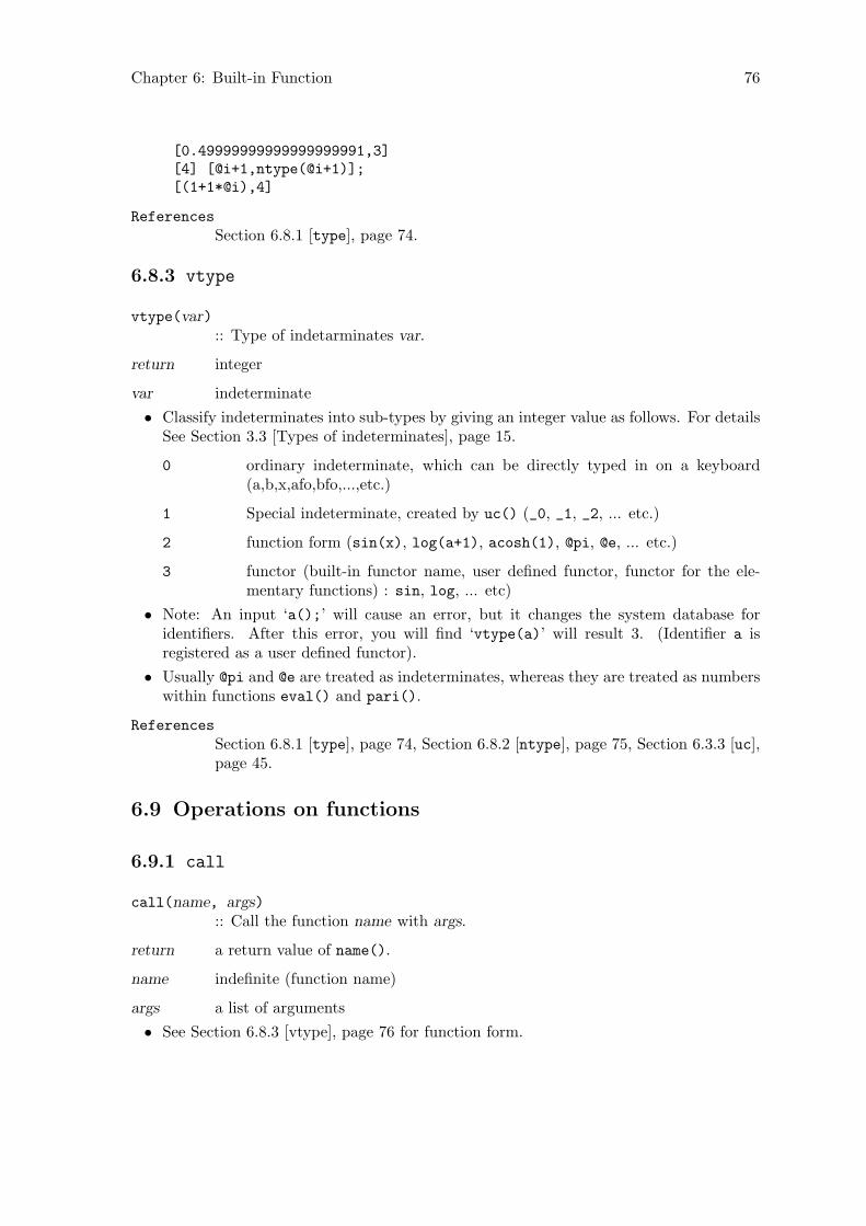
Chapter 6: Built-in Function 76
[0.49999999999999999991,3][4] [@i+1,ntype(@i+1)];[(1+1*@i),4]
References
Section 6.8.1 [type], page 74.
6.8.3 vtype
vtype(var):: Type of indetarminates var.
return integer
var indeterminate
• Classify indeterminates into sub-types by giving an integer value as follows. For detailsSee Section 3.3 [Types of indeterminates], page 15.
0 ordinary indeterminate, which can be directly typed in on a keyboard(a,b,x,afo,bfo,...,etc.)
1 Special indeterminate, created by uc() (_0, _1, _2, ... etc.)
2 function form (sin(x), log(a+1), acosh(1), @pi, @e, ... etc.)
3 functor (built-in functor name, user defined functor, functor for the ele-mentary functions) : sin, log, ... etc)
• Note: An input ‘a();’ will cause an error, but it changes the system database foridentifiers. After this error, you will find ‘vtype(a)’ will result 3. (Identifier a isregistered as a user defined functor).
• Usually @pi and @e are treated as indeterminates, whereas they are treated as numberswithin functions eval() and pari().
References
Section 6.8.1 [type], page 74, Section 6.8.2 [ntype], page 75, Section 6.3.3 [uc],page 45.
6.9 Operations on functions
6.9.1 call
call(name, args):: Call the function name with args.
return a return value of name().
name indefinite (function name)
args a list of arguments
• See Section 6.8.3 [vtype], page 76 for function form.

Chapter 6: Built-in Function 77
[0] A=igcd;igcd[1] call(A,[4,6]);2[2] (*A)(4,6);2
References
Section 6.8.3 [vtype], page 76.
6.9.2 functor, args, funargs
functor(func):: Functor of function form func.
args(func):: List of arguments of function form func.
funargs(func):: cons(functor(func),args(func)).
return functor() : indeterminate, args(), funargs() : list
func function form
• See Section 6.8.3 [vtype], page 76 for function form.
• Extract the functor and the arguments of function form func.
• Assign a program variable, say F, to the functor obtained by functor(). Then, youcan type (*F)(x) (, or (*F)(x,y,...) depending on the arity,) to input a function formwith argument x.
[0] functor(sin(x));sin[0] args(sin(x));[x][0] funargs(sin(3*cos(y)));[sin,3*cos(y)][1] for (L=[sin,cos,tan];L!=[];L=cdr(L)) {A=car(L);print(eval((*A)(@pi/3)));}0.866025403491221368310.50000000021.7320508058
References
Section 6.8.3 [vtype], page 76.
6.10 Strings
6.10.1 rtostr
rtostr(obj):: Convert obj into a string.

Chapter 6: Built-in Function 78
return string
obj arbitrary
• Convert an arbitrary object obj into a string.
• This function is convenient to create variables with numbered (or indexed) names byconverting integers into strings and appending them to some name strings.
• Use strtov() for inverse conversion from string to indeterminate.
[0] A=afo;afo[1] type(A);2[2] B=rtostr(A);afo[3] type(B);7[4] B+"1";afo1
References
Section 6.10.2 [strtov], page 78, Section 6.8.1 [type], page 74.
6.10.2 strtov
strtov(str):: Convert a string str into an indeterminate.
return intederminate
str string which is valid to constitute an indeterminate.
• Convert a string that is valid for an indeterminate into an indeterminate which havestr as its print name.
• The valid string for an indeterminate is such a string that begins with a small alpha-betical letter possibly followed by any string composed of alphabetical letters, digits ora symbol ‘_’.
• Use the command to create indeterminates dynamically in programs.
[0] A="afo";afo[1] for (I=0;I<3;I++) {B=strtov(A+rtostr(I)); print([B,type(B)]);}[afo0,2][afo1,2][afo2,2]
References
Section 6.10.1 [rtostr], page 77, Section 6.8.1 [type], page 74, Section 6.3.3[uc], page 45.
6.10.3 eval_str

Chapter 6: Built-in Function 79
eval_str(str):: Evaluates a string str.
return object
str string which can be accepted by Asir parser
• This function evaluates a string which can be accepted by Asir parser and returns theresult.
• The input string should represent an expression.
• This functions is the inversion function of rtostr().
[0] eval_str("1+2");3[1] fctr(eval_str(rtostr((x+y)^10)));[[1,1],[x+y,10]]
References
Section 6.10.1 [rtostr], page 77
6.10.4 strtoascii, asciitostr
strtoascii(str):: Converts a string into a sequence of ASCII codes.
asciitostr(list):: Converts a sequence of ASCII codes into a string.
return strtoascii():list; asciitostr():string
str string
list list containing positive integers less than 256.
• strtoascii() converts a string into a list of integers which is a representation of thestring by the ASCII code.
• asciitostr() is the inverse of asciitostr().
[0] strtoascii("abcxyz");[97,98,99,120,121,122][1] asciitostr(@);abcxyz[2] asciitostr([256]);asciitostr : argument out of rangereturn to toplevel
6.10.5 str_len, str_chr, sub_str
str_len(str):: Returns the length of a string.
str_chr(str,start,c):: Returns the position of the first occurrence of a character in a string.
sub_str(str,start,end):: Returns a substring of a string.

Chapter 6: Built-in Function 80
return str_len(), str_chr():integer; sub_str():string
str c string
start end non-negative integer
• str_len() returns the length of a string.
• str_chr() scans a string str from the start-th character and returns the position ofthe first occurrence of the first character of a string c. Note that the top of a string isthe 0-th charater. It returns -1 if the character does not appear.
• sub_str() generates a substring of str containing characters from the start-th one tothe end-th one.
[185] Line="123 456 (x+y)^3";123 456 (x+y)^3[186] Sp1 = str_chr(Line,0," ");3[187] D0 = eval_str(sub_str(Line,0,Sp1-1));123[188] Sp2 = str_chr(Line,Sp1+1," ");7[189] D1 = eval_str(sub_str(Line,Sp1+1,Sp2-1));456[190] C = eval_str(sub_str(Line,Sp2+1,str_len(Line)-1));x^3+3*y*x^2+3*y^2*x+y^3
6.11 Inputs and Outputs
6.11.1 end, quit
end, quit
:: Close the currently reading file. At the top level, terminate the Asir session.
• These two functions take no arguments. These functions can be called without a ‘()’.Either function close the current input file. This means the termination of the Asirsession at the top level.
• An input file will be automatically closed if it is read to its end. However, if no end$
is written at the last of the input file, the control will be returned to the top leveland Asir will be waiting for an input without any prompting. Thus, in order to avoidconfusion, putting a end$ at the last line of the input file is strongly recommended.
[6] quit;%
References
Section 6.11.2 [load], page 80.
6.11.2 load
load("filename"):: Reads a program file filename.

Chapter 6: Built-in Function 81
return (1|0)
filename file (path) name
• See Chapter 4 [User language Asir], page 17 for practical programming. Since text filesare read through cpp, the user can use, as in C programs, #include and #define inAsir program source codes.
• It returns 1 if the designated file exists, 0 otherwise.
• If the filename begins with ‘/’, it is understood as an absolute path name; with ‘.’,relative path name from current directory; otherwise, the file is searched first fromdirectories assigned to an environmental variable ASIRLOADPATH, then if the search endsup in failure, the standard library directory (or directories assigned to ASIR_LIBDIR)shall be searched. On Windows, get_rootdir()/lib is searched if ASIR_LIBDIR is notset.
• We recommend to write an end command at the last line of your program. If not, Asirwill not give you a prompt after it will have executed load command. (Escape withan interrupt character (Section 2.7 [Interruption], page 8), if you have lost yourself.)Even in such a situation, Asir itself is still ready to read keyboard inputs as usual. Itis, however, embarrassing and may cause other errors. Therefore, to put an end$ atthe last line is desirable. (Command end; will work as well, but it also returns anddisplays verbose.)
• On Windows one has to use ‘/’ as the separator of directory names.
References
Section 6.11.1 [end quit], page 80, Section 6.11.3 [which], page 81,Section 6.14.16 [get_rootdir], page 97.
6.11.3 which
which("filename"):: This returns the path name for the filename which load() will read.
return path name
filename filename (path name) or 0
• This function searches directory trees according to the same procedure as load() willdo. Then, returns a string, the path name to the file if the named file exists; 0 unlessotherwise.
• For details of searching procedure, refer to the description about load().
• On Windows one has to use ‘/’ as the separator of directory names.
[0] which("gr");./gb/gr[1] which("/usr/local/lib/gr");0[2] which("/usr/local/lib/asir/gr");/usr/local/lib/asir/gr
References
Section 6.11.2 [load], page 80.

Chapter 6: Built-in Function 82
6.11.4 output
output(["filename"]):: Writes the return values and prompt onto file filename.
return 1
filename filename
• Standard output stream of Asir is redirected to the specified file. While Asir is writ-ing its outputs onto a file, no outputs, except for keyboard inputs and some of errormessages, are written onto the standard output. (You cannot see the result on thedisplay.)
• To direct the Asir outputs to the standard output, issue the command without argu-ment, i.e., output().
• If the specified file already exists, new outputs will be added to the tail of the file. Ifnot, a file is newly created and the outputs will be written onto the file.
• When file name is specified without double quotes (""), or when protected file is spec-ified, an error occurs and the system returns to the top level.
• If you want to write inputs from the key board onto the file as well as Asir outputs,put command ctrl("echo",1), and then redirect the standard output to your desiredfile.
• Contents which are written onto the standard error output, CPU time etc., are notwritten onto the file.
• Reading and writing algebraic expressions which contain neither functional forms norunknown coefficients (vtype() References) are performed more efficiently, with respectto both time and space, by bload() and bsave().
• On Windows one has to use ‘/’ as the separator of directory names.
[83] output("afo");fctr(x^2-y^2);print("afo");output();1[87] quit;% cat afo1[84] [[1,1],[x+y,1],[x-y,1]][85] afo0[86]
References
Section 6.14.1 [ctrl], page 89, Section 6.11.5 [bsave bload], page 82.
6.11.5 bsave, bload
bsave(obj,"filename"):: This function writes obj onto filename in binary form.

Chapter 6: Built-in Function 83
bload("filename"):: This function reads an expression from filename in binary form.
return bsave() : 1, bload() : the expression read
obj arbitrary expression which does not contain neither function forms nor unknowncoefficients.
filename filename
• Function bsave() writes an object onto a file in its internal form (not exact internalform but very similar). Function bload() read the expression from files which is writtenby bsave(). Current implementation support arbitrary expressions, including lists,arrays (i.e., vectors and matrices), except for function forms and unknown coefficients(vtype() References.)
• The parser is activated to retrieve expressions written by output() , whereas internalforms are directly reconstructed by bload() from the bsave()’ed object in the file.The latter is much more efficient with respect to both time and space.
• It may happen that the variable ordering at reading is changed from that at writing. Insuch a case, the variable ordering in the internal expression is automatically rearrangedaccording to the current variable ordering.
• On Windows one has to use ‘/’ as the separator of directory names.
[0] A=(x+y+z+u+v+w)^20$[1] bsave(A,"afo");1[2] B = bload("afo")$[3] A == B;1[4] X=(x+y)^2;x^2+2*y*x+y^2[5] bsave(X,"afo")$[6] quit;% asir[0] ord([y,x])$[1] bload("afo");y^2+2*x*y+x^2
References
Section 6.11.4 [output], page 82.
6.11.6 bload27
bload27("filename"):: Reads bsaved file created by older version of Asir.
return expression read
filename filename
• In older versions an arbitrary precision integer is represented as an array of 27bitintegers. In the current version it is represented as an array of 32bit integers. By thisincompatibility the bsaved file created by older versions cannot be read in the currentversion by bload. bload27 is used to read such files.

Chapter 6: Built-in Function 84
• On Windows one has to use ‘/’ as the separator of directory names.
References
Section 6.11.5 [bsave bload], page 82.
6.11.7 print
print(obj [,nl]):: Displays (or outputs) obj.
return 0
obj arbitrary
nl flag (arbitrary)
• Displays (or outputs) obj.
• It normally adds linefeed code to cause the cursor moving to the next line. If 0 or 2 isgiven as the second argument, it does not add a linefeed. If the second argument is 0,the output is simply written in the buffer. If the second argument is 2, the output isflushed.
• The return value of this function is 0. If command print(rat); is performed at thetop level, first the value of rat will be printed, followed by a linefeed, followed by a 0which is the value of the function and followed by a linefeed and the next prompt. (Ifthe command is terminated by a ‘$’, e.g., print(rat)$, The last 0 will not be printed.)
• Formatted outputs are not currently supported. If one wishes to output multiple objectsby a single print() command, use list like [obj1,...], which is not so beautiful, butconvenient to minimize programming efforts.
[8] def cat(L) { while ( L != [] ) { print(car(L),0); L = cdr(L);}print(""); }[9] cat([xyz,123,"gahaha"])$xyz123gahaha
6.11.8 access
access(file):: testing an existence of file.
return (1|0)
file filename
6.11.9 remove_file
remove_file(file):: Delete an file file.
return 1
file filename

Chapter 6: Built-in Function 85
6.11.10 open_file, close_file, get_line, get_byte, put_byte, purge_stdin
open_file("filename"[,"mode"]):: Opens filename for reading.
close_file(num)
:: Closes the file indicated by a descriptor num.
get_line([num])
:: Reads a line from the file indicated by a descriptor num.
get_byte(num)
:: Reads a byte from the file indicated by a descriptor num.
put_byte(num,c):: Writes a byte c to the file indicated by a descriptor num.
purge_stdin()
:: Clears the buffer for the standard input.
return open_file() : integer (fild id); close_file() : 1; get_line() : string; get_byte(), put_byte() : integer
filename file (path) name
mode string
num non-negative integer (file descriptor)
• open_file() opens a file. If mode is not specified, a file is opened for reading. If modeis specified, it is used as the mode specification for C standard I/O function fopen().For example "w" requests that the file is truncated to zero length or created for writing."a" requests that the file is opened for writing or created if it does not exist. The streampointer is set at the end of the file. If successful, it returns a non-negative integer as thefile descriptor. Otherwise the system error function is called. Unnecessary files shouldbe closed by close_file(). If the special file name unix://stdin or unix://stdoutor unix://stderr is given, it returns the file descriptor for the standard input or thestandard output or the standard error stream respectively. The mode argument isignored in this case.
• get_line() reads a line from an opened file and returns the line as a string. If noargument is supplied, it reads a line from the standard input.
• get_byte() reads a byte from an opened file and returns the it as an integer.
• put_byte() writes a byte from an opened file and returns the the byte as an integer.
• A get_line() call after reading the end of file returns an integer 0.
• Strings can be converted into internal forms with string manipulation functions suchas sub_str(), eval_str().
• purge_stdin() clears the buffer for the standard input. When a function receives acharacter string from get_line(), this functions should be called in advance in orderto avoid an incorrect behavior which is caused by the characters already exists in thebuffer.

Chapter 6: Built-in Function 86
[185] Id = open_file("test");0[186] get_line(Id);12345
[187] get_line(Id);67890
[188] get_line(Id);0[189] type(@@);0[190] close_file(Id);1[191] open_file("test");1[192] get_line(1);12345
[193] get_byte(1);54 /* the ASCII code of ’6’ */[194] get_line(1);7890 /* the rest of the last line */[195] def test() { return get_line(); }[196] def test1() { purge_stdin(); return get_line(); }[197] test();
/* a remaining newline character has been read *//* returns immediately */
[198] test1();123; /* input from a keyboard */123; /* returned value */
[199]
References
Section 6.10.3 [eval_str], page 78, Section 6.10.5 [str_len str_chr sub_str],page 79.
6.12 Operations for modules
6.12.1 module_list
module_list()
:: Get the list of loaded modules.
return The list of loaded modules.
[1040] module_list();[gr,primdec,bfct,sm1,gnuplot,tigers,phc]

Chapter 6: Built-in Function 87
References
See Section 4.2.13 [module], page 27.
6.12.2 module_definedp
module_definedp(name):: Testing an existense of the module name.
return (1|0)
name a module name
• If the module name exists, then module_definedp returns 1. othewise 0.
[100] module_definedp("gr");1
References
Section 6.12.1 [module_list], page 86, See Section 4.2.13 [module], page 27.
6.12.3 remove_module
remove_module(name):: Remove the module name.
return (1|0)
name a module name
•[100] remove_module("gr");1
References
See Section 4.2.13 [module], page 27.
6.13 Numerical functions
6.13.1 dacos, dasin, datan, dcos, dsin, dtan
dacos(num)
:: Get the value of Arccos of num.
dasin(num)
:: Get the value of Arcsin of num.
datan(num)
:: Get the value of Arctan of num.
dcos(num)
:: Get the value of cos of num.
dsin(num)
:: Get the value of sin of num.
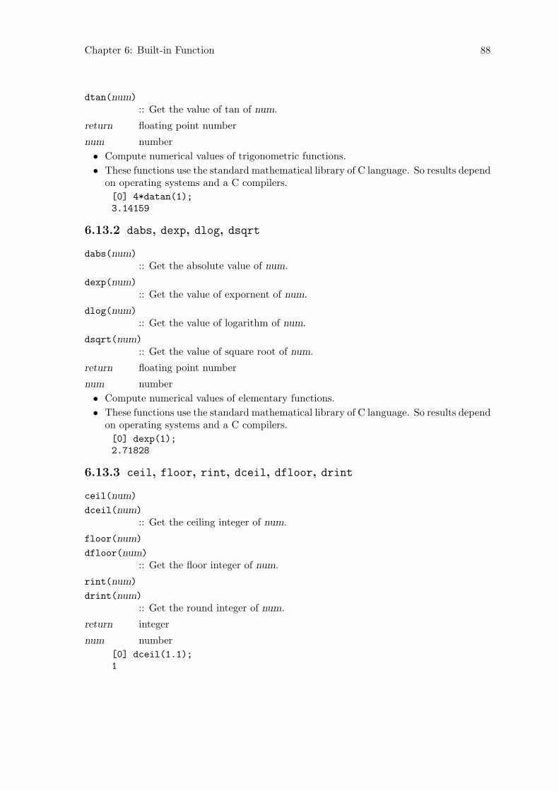
Chapter 6: Built-in Function 88
dtan(num)
:: Get the value of tan of num.
return floating point number
num number
• Compute numerical values of trigonometric functions.
• These functions use the standard mathematical library of C language. So results dependon operating systems and a C compilers.
[0] 4*datan(1);3.14159
6.13.2 dabs, dexp, dlog, dsqrt
dabs(num)
:: Get the absolute value of num.
dexp(num)
:: Get the value of expornent of num.
dlog(num)
:: Get the value of logarithm of num.
dsqrt(num)
:: Get the value of square root of num.
return floating point number
num number
• Compute numerical values of elementary functions.
• These functions use the standard mathematical library of C language. So results dependon operating systems and a C compilers.
[0] dexp(1);2.71828
6.13.3 ceil, floor, rint, dceil, dfloor, drint
ceil(num)
dceil(num)
:: Get the ceiling integer of num.
floor(num)
dfloor(num)
:: Get the floor integer of num.
rint(num)
drint(num)
:: Get the round integer of num.
return integer
num number
[0] dceil(1.1);1

Chapter 6: Built-in Function 89
6.14 Miscellaneouses
6.14.1 ctrl
ctrl("switch"[,obj]):: Sets the value of switch.
return value of switch
switch switch name
obj parameter
• This function is used to set or to get the values of switches. The switches are used tocontrol an execution of Asir.
• If obj is not specified, the value of switch is returned.
• If obj is specified, the value of switch is set to obj.
• Switches are specified by strings, namely, enclosed by two double quotes.
• Here are of switches of Asir.
cputime If ‘on’, CPU time and GC time is displayed at every top level evaluationof Asir command; if ‘off’, not displayed. See Section 6.14.6 [cputime tstarttstop], page 92. (The switch is also set by command cputime(1), and resetby cputime(0).)
nez Selection for EZGCD algorithm. It is set to 1 by default. Ordinary usersneed not change this setting.
echo If ‘on’, inputs from the standard input will be echoed onto the standardoutput. When executing to load a file, the contents of the file will bewritten onto the standard output. If ‘off’, the inputs will not be echoed.This command will be useful when used with command output.
bigfloat If ‘on’, floating operations will be done by PARI system with arbitraryprecision floating point operations. Default precision is set to 9 digits. Tochange the precision, use command setprec. If ‘off’, floating operationswill be done by Asir’s own floating operation routines with a fixed precisionoperations of standard floating double.
adj Sets the frequency of garbage collection. A rational number greater than orequal to 1 can be specified. The default value is 3. If a value closer to 1 isspecified, larger heap is allocated and as a result, the frequency of garbagecollection decreases. See Section 2.4 [Command line options], page 5.
verbose If ‘on’ a warning messages is displayed when a function is redefined.
quiet_mode
If 1 is set, the copyright notice has been displayed at boot time.
prompt If the value is 0, then prompt is not output. If the value is 1,then the standard prompt is output. Asir prompt can be cus-tomized by giving a C-style format string. Example (for unix asir);ctrl("prompt","\033[32m[%d]:= \033[0m")

Chapter 6: Built-in Function 90
hex If 1 is set, integers are displayed as hexadecimal numbers with prefix 0x.if -1 is set, hexadecimal numbers are displayed with ‘|’ inserted at every 8hexadecimal digits.
real_digit
Sets the number of digits used to print a floating double.
double_output
If set to 1, any floating double is printed in the style ddd.ddd.
fortran_output
If ‘on’ polynomials are displayed in FORTRAN style. That is, a power isrepresented by ‘**’ instead of ‘^’. The default value is ’off.
ox_batch If ’on’, the OpenXM send buffer is flushed only when the buffer is full. If’off’, the buffer is always flushed at each sending of data or command. Thedefault value is ’off’. See Chapter 7 [Distributed computation], page 99.
ox_check If ’on’ the check by mathcap is done before sending data. The default valueis ’on’. See Chapter 7 [Distributed computation], page 99.
ox_exchange_mathcap
If ’on’ Asir forces the exchange of mathcaps at the communication startup.The default value is ’on’. See Chapter 7 [Distributed computation], page 99.
References
Section 6.14.6 [cputime tstart tstop], page 92, Section 6.11.4 [output],page 82, Section 6.1.14 [pari], page 40, Section 6.1.15 [setprec], page 41,Section 6.1.13 [eval deval], page 39.
6.14.2 debug
debug :: Forces to enter into debugging mode.
Function debug is a function with no argument. It can be called without ‘()’.
• In the debug-mode, you are prompted by (debug) and the debugger is ready for com-mands. Typing in quit (Note! without a semicolon.) brings you to exit the debug-mode.
• See Chapter 5 [Debugger], page 30 for details.
[1] debug;(debug) quit0[2]
6.14.3 error
error(message):: Forces Asir to cause an error and enter debugging mode.
message string

Chapter 6: Built-in Function 91
• When Asir encounters a serious error such that it finds difficult to continue execution,it, in general, tries to enter debugging mode before it returns to top level. The commanderror() forces a similar behavior in a user program.
• The argument is a string which will be displayed when error() will be executed.
• You can enter the debug-mode when your program encounters an illegal value for aprogram variable, if you have written the program so as to call error() upon findingsuch an error in your program text.
% cat mod3def mod3(A) {
if ( type(A) >= 2 )error("invalid argument");
elsereturn A % 3;
}end$% asir[0] load("mod3");1[3] mod3(5);2[4] mod3(x);invalid argumentstopped in mod3 at line 3 in file "./mod3"3 error("invalid argument");(debug) print AA = x(debug) quitreturn to toplevel[4]
References
Section 6.14.2 [debug], page 90.
6.14.4 help
help(["function"]):: Displays the description of function function.
return 0
function function name
• If invoked without argument, it displays rough usage of Asir.
• If a function name is given and if there exists a file with the same name in the directory‘help’ under standard library directory, the file is displayed by a command set to theenvironmental variable PAGER or else command ‘more’.
• If the LANG environment variable is set and its value begins with "japan" or "ja_JP",then the file in ‘help-ja’ is displayed. If its value does not begin with "japan" or"ja_JP", then the file in ‘help-en’ is displayed.
• On Windows HTML-style help is available from the menu.

Chapter 6: Built-in Function 92
6.14.5 time
time() :: Returns a four element list consisting of total CPU time, GC time, the elapsedtime and also total memory quantities requested from the start of current Asirsession.
return list
• These are commands regarding CPU time and GC time.
• The GC time is the time regarded to spent by the garbage collector, and the CPUtime is the time defined by subtracting the GC time from the total time consumed bycommand Asir. Their unit is ‘second.’
• Command time() returns total CPU time and GC time measured from the start ofcurrent Asir session. It also returns the elapsed time. Time unit is ‘second.’ Moreover,it returns total memory quantities in words (usually 4 bytes) which are requested tothe memory manager from the beginning of the current session. The return value is alist and the format is [CPU time, GC time, Memory, Elapsed time].
• You can find the CPU time and GC time for some computation by taking the differenceof the figure reported by time() at the beginning and the ending of the computation.
• Since arbitrary precision integers are NOT used for counting the total amount of mem-ory request, the number will eventually happen to become meaningless due to integeroverflow.
• When cputime switch is active by ctrl() or by cputime(), the execution time will bedisplayed after every evaluation of top level statement. In a program, however, in orderto know the execution time for a sequence of computations, you have to use time()
command, for an example.
• On UNIX, if getrusage() is available, time() reports reliable figures. On WindowsNT it also gives reliable CPU time. However, on Windows 95/98, the reported timeis nothing but the elapsed time of the real world. Therefore, the time elapsed in thedebug-mode and the time of waiting for a reply to interruption prompting are addedto the elapsed time.
[72] T0=time();[2.390885,0.484358,46560,9.157768][73] G=hgr(katsura(4),[u4,u3,u2,u1,u0],2)$[74] T1=time();[8.968048,7.705907,1514833,63.359717][75] ["CPU",T1[0]-T0[0],"GC",T1[1]-T0[1]];[CPU,6.577163,GC,7.221549]
References
Section 6.14.6 [cputime tstart tstop], page 92, Section 6.14.8 [currenttime],page 94.
6.14.6 cputime, tstart, tstop
cputime(onoff ):: Stop displaying cputime if its argument is 0, otherwise start displayingcputime after every top level evaluation of Asir command.

Chapter 6: Built-in Function 93
tstart() :: Resets and starts timer for CPU time and GC time.
tstop() :: Stops timer and then displays CPU time GC time elapsed from the last timewhen timer was started.
return 0
onoff flag (arbitrary)
• Command cputime() with NON-ZERO argument enables Asir to display CPU timeand GC time after every evaluation of top level Asir command. The command withargument 0 disables displaying them.
• Command tstart() starts measuring CPU time and GC time without arguments. Theparentheses ‘()’ may be omitted.
• Command tstop() stops measuring CPU time and GC time and displays them withoutarguments. The parentheses ‘()’ may be omitted.
• Command cputime(onoff ) has same meaning as ctrl("cputime",onoff ).
• Nested use of tstart() and tstop() is not expected. If such an effect is desired, usetime().
• On and off states by cputime() have effects only to displaying mode. Time for eval-uation of every top level statement is always measured. Therefore, even after a com-putation has already started, you can let Asir display the timings, whenever you enterthe debug-mode and execute cputime(1).
[49] tstart$[50] fctr(x^10-y^10);[[1,1],[x+y,1],[x^4-y*x^3+y^2*x^2-y^3*x+y^4,1],[x-y,1],[x^4+y*x^3+y^2*x^2+y^3*x+y^4,1]][51] tstop$80msec + gc : 40msec
References
Section 6.14.5 [time], page 92, Section 6.14.8 [currenttime], page 94, Sec-tion 6.14.1 [ctrl], page 89.
6.14.7 timer
timer(interval,expr,val):: Compute an expression under the interval timer.
return result
interval interval (second)
expr expression to be computed
val a value to be returned when the timer is expired
• timer() computes an expression under the interval timer. If the computation finisheswithin the specified interval, it returns the result of the computation. Otherwise itreturns the third argument.
• The third argument should be distinguishable from the result on success.

Chapter 6: Built-in Function 94
[0] load("cyclic");1[10] timer(10,dp_gr_main(cyclic(7),[c0,c1,c2,c3,c4,c5,c6],1,1,0),0);interval timer expired (VTALRM)0[11]
6.14.8 currenttime
currenttime()
:: Get current time.
return UNIX time.
• See also time(3) in UNIX manuals.
[0] currenttime();1071639228[1]
6.14.9 sleep
sleep(interval):: Suspend computation for an interval.
return 1
interval interval (micro second)
• See also usleep(3) in UNIX manuals.
[0] sleep(1000);1[1]
6.14.10 heap
heap() :: Heap area size currently in use.
return non-negative integer
• Command heap() returns an integer which is the byte size of current Asir heap area.
Heap is a memory area where various data for expressions and user programs of Asirand is managed by the garbage collector. While Asir is running, size of the heap ismonotonously non-decreasing against the time elapsed. If it happens to exceed the realmemory size, most (real world) time is consumed for swapping between real memoryand disk memory.
• For a platform with little real memory, it is recommended to set up Asir configurationtuned for GC functions by -adj option at the activation of Asir. (See Section 2.4[Command line options], page 5.)
% asir -adj 16[0] load("fctrdata")$0

Chapter 6: Built-in Function 95
[97] cputime(1)$0msec[98] heap();5242880msec[99] fctr(Wang[8])$3.190sec + gc : 3.420sec[100] heap();11182080msec[101] quit;% asir[0] load("fctrdata")$0[97] cputime(1)$0msec[98] heap();8273920msec[99] fctr(Wang[8])$3.000sec + gc : 1.180sec[100] heap();16261120msec[101] quit;
References
Section 2.4 [Command line options], page 5.
6.14.11 version
version()
:: Version identification number of Asir.
return integer
• Command version() returns the version identification number, an integer of Asir inuse.
[0] version();991214
6.14.12 shell
shell(command):: Execute shell commands described by a string command.
return integer
command string
Execute shell commands described by a string command by a C function system().This returns the exit status of shell as its return value.

Chapter 6: Built-in Function 96
[0] shell("ls");alg da katsura ralg suitalgt defs.h kimura ratint testalpi edet kimura3 robot texput.logasir.o fee mfee sasa wangasir_symtab gr mksym shira wang_database gr.h mp snf1 wtbgk help msubst solvechou hom p spconst ifplot proot strumcyclic is r sugar0[1]
6.14.13 map
map(function,arg0,arg1,...):: Applies a function to each member of a list or an array.
return an object of the same type as arg0.
function the name of a function
arg0 list, vector or matrix
arg1 ... arbitrary (the rest of arguments)
• Returns an object of the same type as arg0. Each member of the returned object isthe return value of a function call where the first argument is the member of arg0corresponding to the member in the returned object and the rest of the argument arearg1, . . . .
• function is a function name itself without ‘"’.
• A program variable cannot be used as function.
• If arg0 is neither list nor array this function simply returns the value offunction(arg0,arg1,. . . ).
[82] def afo(X) { return X^3; }[83] map(afo,[1,2,3]);[1,8,27]
6.14.14 flist
flist() :: Returns the list of function names currently defined.
return list of character strings
• Returns the list of names of built-in functions and user defined functions currentlydefined. The return value is a list of character strings.
• The names of built-in functions are followed by those of user defined functions.
[77] flist();[defpoly,newalg,mainalg,algtorat,rattoalg,getalg,alg,algv,...]

Chapter 6: Built-in Function 97
6.14.15 delete_history
delete_history([index]):: Deletes the history.
return 0
index Index of history to be deleted.
• Deletes all the histories without an argument.
• Deletes the history with index index if specified.
• A history is an expression which has been obtained by evaluating an input given for aprompt with an index. It can be taken out by @index, which means that the expressionsurvives garbage collections.
• A large history may do harm in the subsequent memory management and deleting thehistory by delete_history(), after saving it in a file by bsave(), is often effective.
[0] (x+y+z)^100$[1] @0;...[2] delete_history(0);[3] @0;0
6.14.16 get_rootdir
get_rootdir()
:: Gets the name of Asir root directory.
return string
• On UNIX it returns the value of an environment variable ASIR_LIBDIR or‘/usr/local/lib/asir’ if ASIR_LIBDIR is not set.
• On Windows the name of Asir root directory is returned.
• By using relative path names from the value of this function, one can write programswhich contain file operations independent of the install directory.
6.14.17 getopt
getopt([key]):: Returns the value of an option.
return object
• When a user defined function is called, the number of arguments must be equal to thatin the declaration of the function. A function with indefinite number of argumentscan be realized by using options (see Section 4.2.12 [option], page 26). The value of aspecified option is retrieved by getopt.
• If getopt() is called with no argument, then it returns a list [[key1,value1],
[key2,value2],...]. In the list, each key is an option which was specified when thefunction executing getopt was invoked, and value is the value of the option.

Chapter 6: Built-in Function 98
• If an option key is specified upon a function call, getopt return the value of the option.If such an option is not specified, the it returns an object of VOID type whose objectidentifier is -1. By examining the type of the returned value with type(), one knowswhether the option is set or not.
• Options are specified as follows:
xxx(A,B,C,D|x=X,y=Y,z=Z)
That is, the options are specified by a sequence of key=value seperated by ‘,’, after‘|’.
References
Section 4.2.12 [option], page 26, Section 6.8.1 [type], page 74.
6.14.18 getenv
getenv(name):: Returns the value of an environment variable.
returnname string
• Returns the value of an environment variable name.
[0] getenv("HOME");/home/pcrf/noro

Chapter 7: Distributed computation 99
7 Distributed computation
7.1 OpenXM
On Asir distributed computations are done under OpenXM (Open message eXchangeprotocol for Mathematics), which is a protocol for exchanging mainly mathematical objectsbetween processes. See http://www.math.sci.kobe-u.ac.jp/OpenXM/ for the details ofOpenXM. In OpenXM a distributed computation is done as follows:
1. A client requests something to a server.
2. The server does works according to the request.
3. The client requests to send data to the server.
4. The server sends the data to the client and the client gets the data.
The server is a stack machine. That is data objects sent by the client are pushed to thestack of the server. If the server gets a command, then the data are popped form the stackand they are used as arguments of a function call.
In OpenXM, the result of a computation done in the server is simply pushed to the stackand the data is not written to the communication stream without requests from the client.
OpenXM protocol consists of two components: CMO (Common Mathematical Objectformat) which determines a common format of data representations and SM (StackMachinecommand) which specifies actions on servers. These are wrapped as OX expressions toindicate the sort of data when they are sent.
To execute a distributed computation by OpenXM, one has to invoke OpenXM serversand to establish communications between the client and the servers. ox_launch(), ox_launch_nox(), ox_launch_generic() are preprared for such purposes. Furthermore thefollowing functions are available.
ox_push_cmo()
It requests a server to push an object to the stack of a server.
ox_pop_cmo()
It request a server to pop an object from the stack of a server.
ox_cmo_rpc()
It requests to execute a function on a server. The result is pushed to the stackof the server.
ox_execute_string()
It requests a server to parse and execute a string by the parser and the evaluaterof the server. The result is pushed to the stack of the server.
ox_push_cmd()
It requests a server to execute a command.
ox_get()
It gets an object from a data stream.

Chapter 7: Distributed computation 100
7.2 Mathcap
A server or a client does not necessarily implement full specifications of OpenXM. If aprogram sends data unknown to its peer, an unrecoverable error may occur. To avoid sucha case OpenXM provides a scheme not to send data unknown to peers. It is realized byexchanging the list of supported CMO and SM. The list is called mathcap. Mathcap is alsodefined as a CMO and the elements are 32bit integers or strings. The format of mathcapis as follows.
[[version number, server name],SMtaglist, [[OXtag,CMOtaglist],[OXtag,CMOtaglist],...]]
[OXtag,CMOtaglist] indicates that available object tags for a category of data specifiedby OXtag. For example ‘ox_asir’ accepts the local object format used by Asir and themathcap from ‘ox_asir’ reflects the fact.
If "ox_check" switch of ctrl is set to 1, the check by a mathcap is done before data issent. If "ox_check" switch of ctrl is set to 0, the check is not done. By default it is set to1.
7.3 Stackmachine commands
The stackmachine commands are provided to request a server to execute various opera-tions. They are automatically sent by built-in functions of Asir, but one often has to sendthem manually. They are represented by 32bit integers. One can send them by callingox_push_cmd(). Typical stackmachine commands are as follows. SM xxx=yyy means thatSM xxx is a mnemonic and that yyy is its value.
SM popSerializedLocalObject=258An object not necessarily defined as CMO is popped from the stack and is sentto the client. This is available only on ‘ox_asir’.
SM popCMO=262A CMO object is popped from the stack and is sent to the client.
SM popString=263An object is popped from the stack and is sent to the client as a readable string.
SM mathcap=264The server’s mathcap is pushed to the stack.
SM pops=265Objects are removed from the stack. The number of object to be removed isspecified by the object at the top of the stack.
SM setName=266A variable name is popped form the stack. Then an object is popped and it isassigned to the variable. This assignment is done by the local language of theserver.
SM evalName=267A variable name is popped from the stack. Then the value of the variable ispushed to the stack.

Chapter 7: Distributed computation 101
SM executeStringByLocalParser=268A string popped from the stack is parsed and evaluated. The result is pushedto the stack.
SM executeFunction=269A function name, the number of arguments and the arguments are popped fromthe stack. Then the function is executed and the result is pushed to the stack.
SM beginBlock=270It indicates the beginning of a block.
SM endBlock=271It indicates the end of a block.
SM shutdown=272It shuts down communications and terminates servers.
SM setMathcap=273It requests a server to register the data at the top of the stack as the client’smathcap.
SM getsp=275The number of objects in the current stack is pushed to the stack.
SM dupErrors=276The list of all the error objects in the current stack is pushed to the stack.
SM nop=300Nothing is done.
7.4 Debugging
In general, it is difficult to debug distributed computations. ‘ox_asir’ provides severalfunctions for debugging.
7.4.1 Error object
When an error has occurred on an OpenXM server, an error object is pushed to thestack instead of a result of the computation. The error object consists of the serial numberof the SM command which caused the error, and an error message.
[340] ox_launch();0[341] ox_rpc(0,"fctr",1.2*x);0[342] ox_pop_cmo(0);error([8,fctrp : invalid argument])
7.4.2 Resetting a server
ox_reset() resets a process whose identifier is number. After its execution the processis ready for receiving data. This function corresponds to the keyboard interrupt on an usualAsir session. It often happens that a request of a client does not correspond correctly to the

Chapter 7: Distributed computation 102
result from a server. It is caused by remaining data on data streams. ox_reset is effectivefor such cases.
7.4.3 Pop-up command window for debugging
As a server does not have any standard input device such as a keyboard, it is difficult todebug user programs running on the server. ‘ox_asir’ pops up a small command windowto input debug commands when an error has occurred during user a program execution orox_rpc(id,"debug") has been executed. The responses to commands are shown in ‘xterm’to display standard outputs from the server. To close the small window, input quit.
7.5 Functions for distributed computation
7.5.1 ox_launch, ox_launch_nox, ox_shutdown
ox_launch([host[,dir],command])ox_launch_nox([host[,dir],command])
:: Initialize OpenXM servers.
ox_shutdown(id):: Terminates OpenXM servers.
return integer
host string or 0
dir commandstring
id integer
• Function ox_launch() invokes a process to execute command on a host host andenables Asir to communicate with that process. If the number of arguments is 3,‘ox_launch’ in dir is invoked on host. Then ‘ox_launch’ invokes command. If host isequal to 0, all the commands are invoked on the same machine as the Asir is running.If no arguments are specified, host, dir and command are regarded as 0, the value ofget_rootdir() and ‘ox_asir’ in the same directory respectively.
• If host is equal to 0, then dir can be omitted. In such a case dir is regarded as thevalue of get_rootdir().
• If command begins with ‘/’, it is regarded as an absolute pathname. Otherwise it isregarded as a relative pathname from dir.
• On UNIX, ox_launch() invokes ‘xterm’ to display standard outputs from command.If X11 is not available or one wants to invoke servers without ‘xterm’, use ox_launch_nox(), where the outputs of command are redirected to ‘/dev/null’. If the environ-ment variable DISPLAY is not set, ox_launch() and ox_launch_nox() behave identi-cally.
• The returned value is used as the identifier for communication.

Chapter 7: Distributed computation 103
• The peers communicating with Asir are not necessarily processes running on the samemachine. The communication will be successful even if the byte order is different fromthose of the peer processes, because the byte order for the communication is determinedby a negotiation between a client and a server.
• The following preparations are necessary. Here, Let A be the host on which Asir isrunning, and B the host on which the peer process will run.
1. Register the hostname of the host A to the ‘~/.rhosts’ of the host B. That is, youshould be allowed to access the host B from A without supplying a password.
2. For cases where connection to X is also used, let Xserver authorize the relevanthosts. Adding the hosts can be done by command xhost.
3. If an environment variable ASIR_RSH is set, the content of this variable is used asa promgram to invoke remote servers instead of rsh. For example,
% setenv ASIR_RSH "ssh -f -X -A "
implies that remote servers are invoked by ‘ssh’ and that X11 forwarding is en-abled. See the manual of ‘ssh’ for the detail.
4. Some command’s consume much stack space. You are recommended to set thestack size to about 16MB large in ‘.cshrc’ for safe. To specify the size, put limitstacksize 16m for an example.
• When command opens a window on X, it uses the string specified for display ; if thespecification is omitted, it uses the value set for the environment variable DISPLAY.
• ox_shutdown() terminates OpenXM servers whose identifier is id.
• When Asir is terminated successfully, all I/O streams are automatically closed, and allthe processes invoked are also terminated. However, some remote processes may notterminated when Asir is terminated abnormally. If ever Asir is terminated abnormally,you have to kill all the unterminated process invoked by Asir on every remote host.Check by ps command on the remote hosts to see if such processed are alive.
• ‘xterm’ for displaying the outputs from command is invoked with ‘-name ox_term’ op-tion. Thus, by specifying resources for the resource name ‘ox_term’, only the behaviourof the ‘xterm’ can be customized.
/* iconify on start */ox_xterm*iconic:on/* activate the scroll bar */ox_xterm*scrollBar:on/* 1000 lines can be shown by the scrollbar */ox_xterm*saveLines:1000
[219] ox_launch();0[220] ox_rpc(0,"fctr",x^10-y^10);0[221] ox_pop_local(0);[[1,1],[x^4+y*x^3+y^2*x^2+y^3*x+y^4,1],[x^4-y*x^3+y^2*x^2-y^3*x+y^4,1],[x-y,1],[x+y,1]][222] ox_shutdown(0);0

Chapter 7: Distributed computation 104
References
Section 7.5.5 [ox_rpc ox_cmo_rpc ox_execute_string], page 106, Sec-tion 7.5.8 [ox_pop_cmo ox_pop_local], page 109, Section 7.5.15 [ifplotconplot plot polarplot plotover], page 113
7.5.2 ox_launch_generic
ox_launch_generic(host,launch,server,use unix,use ssh,use x,conn to serv):: Initialize OpenXM servers.
return integer
host string or 0
launcher serverstring
use unix use ssh use x conn to servinteger
• ox_launch_generic() invokes a control process launch and a server process server onhost. The other arguments are switches for protocol family selection, on/off of the Xenvironment, method of process invocation and selection of connection type.
• If host is equal to 0, processes are invoked on the same machine as the Asir is running.In this case UNIX internal protocol is always used.
• If use unix is equal to 1, UNIX internal protocol is used. If use unix is equal to 0,Internet protocol is used.
• If use ssh is equal to 1,‘ssh’ (Secure Shell) is used to invoke processes. If one doesnot use ‘ssh-agent’, a password (passphrase) is required. If ‘sshd’ is not running onthe target machine, ‘rsh’ is used instead. But it will immediately fail if a password isrequired.
• If use x is equal to 1, it is assumed that X environment is available. In such a caseserver is invoked under ‘xterm’ by using the current DISPLAY variable. If DISPLAY isnot set, it is invoked without X. Note that the processes will hang up if DISPLAY isincorrectly set.
• If conn to serv is equal to 1, Asir (client) executes bind and listen, and the invokedprocesses execute connect. If conn to serv is equal to 0, Asir (client) the invokedprocesses execute bind and listen, and the client executes connect.
[342] LIB=get_rootdir();/export/home/noro/ca/Kobe/build/OpenXM/lib/asir[343] ox_launch_generic(0,LIB+"/ox_launch",LIB+"/ox_asir",0,0,0,0);1[344] ox_launch_generic(0,LIB+"/ox_launch",LIB+"/ox_asir",1,0,0,0);2[345] ox_launch_generic(0,LIB+"/ox_launch",LIB+"/ox_asir",1,1,0,0);3[346] ox_launch_generic(0,LIB+"/ox_launch",LIB+"/ox_asir",1,1,1,0);4[347] ox_launch_generic(0,LIB+"/ox_launch",LIB+"/ox_asir",1,1,1,1);

Chapter 7: Distributed computation 105
5[348] ox_launch_generic(0,LIB+"/ox_launch",LIB+"/ox_asir",1,1,0,1);6
References
Section 7.5.1 [ox_launch ox_launch_nox ox_shutdown], page 102,Section 7.5.2 [ox_launch_generic], page 104
7.5.3 generate_port, try_bind_listen, try_connect, try_accept,register_server
generate_port([use unix]):: Generates a port number.
try_bind_listen(port):: Binds and listens on a port.
try_connect(host,port):: Connects to a port.
try_accept(socket,port):: Accepts a connection request.
register_server(control socket,control port,server socket,server port):: Registers the sockets for which connections are established.
return integer or string for generate_port(), integer for the others
use unix 0 or 1
host string
port control port server portinteger or string
socket control socket server socketinteger
• These functions are primitives to establish communications between a client and servers.
• generate_port() generates a port name for communication. If the argument is notspecified or equal to 0, a port number for Internet domain socket is generated randomly.Otherwise a file name for UNIX domain (host-internal protocol) is generated. Note thatit is not assured that the generated port is not in use.
• try_bind_listen() creates a socket according to the protocol family indicated by thegiven port and executes bind and listen. It returns a socket identifier if it is successful.-1 indicates an error.
• try_connect() tries to connect to a port port on a host host. It returns a socketidentifier if it is successful. -1 indicates an error.
• try_accept() accepts a connection request to a socket socket. It returns a new socketidentifier if it is successful. -1 indicates an error. In any case socket is automaticallyclosed. port is specified to distinguish the protocol family of socket.
• register_server() registers a pair of a control socket and a server socket. A processidentifier indicating the pair is returned. The process identifier is used as an argumentof ox functions such as ox_push_cmo().

Chapter 7: Distributed computation 106
• Servers are invoked by using shell(), or manually.
[340] CPort=generate_port();39896[341] SPort=generate_port();37222[342] CSocket=try_bind_listen(CPort);3[343] SSocket=try_bind_listen(SPort);5
/*ox_launch is invoked here :% ox_launch "127.1" 0 39716 37043 ox_asir "shio:0"*/
[344] CSocket=try_accept(CSocket,CPort);6[345] SSocket=try_accept(SSocket,SPort);3[346] register_server(CSocket,CPort,SSocket,SPort);0
References
Section 7.5.1 [ox_launch ox_launch_nox ox_shutdown], page 102, Sec-tion 7.5.2 [ox_launch_generic], page 104, Section 6.14.12 [shell], page 95,Section 7.5.7 [ox_push_cmo ox_push_local], page 108
7.5.4 ‘ox_asir’
‘ox_asir’ provides almost all the functionalities of Asir as an OpenXM server. ‘ox_asir’is invoked by ox_launch or ox_launch_nox. If X environment is not available or is notnecessary, one can use ox_launch_nox.
[5] ox_launch();0
[5] ox_launch_nox("127.0.0.1","/usr/local/lib/asir","/usr/local/lib/asir/ox_asir");0
[7] RemoteLibDir = "/usr/local/lib/asir/"$[8] Machines = ["sumire","rokkaku","genkotsu","shinpuku"];[sumire,rokkaku,genkotsu,shinpuku][9] Servers = map(ox_launch,Machines,RemoteLibDir,RemoteLibDir+"ox_asir");[0,1,2,3]
References
Section 7.5.1 [ox_launch ox_launch_nox ox_shutdown], page 102
7.5.5 ox_rpc, ox_cmo_rpc, ox_execute_string

Chapter 7: Distributed computation 107
ox_rpc(number,"func",arg0,...)ox_cmo_rpc(number,"func",arg0,...)ox_execute_string(number,"command",...)
:: Calls a function on an OpenXM server
return 0
number integer (process identifier)
func function name
command string
arg0 ... arbitrary (arguments)
• Calls a function on an OpenXM server whose identifier is number.
• It returns 0 immediately. It does not wait the termination of the function call.
• ox_rpc() can be used when the server is ‘ox_asir’. Otherwise ox_cmo_rpc() shouldbe used.
• The result of the function call is put on the stack of the server. It can be received byox_pop_local() or ox_pop_cmo().
• If the server is not ‘ox_asir’, only data defined in OpenXM can be sent.
• ox_execute_string requests the server to parse and execute command by the parserand the evaluater of the server. The result is pushed to the stack.
[234] ox_cmo_rpc(0,"dp_ht",dp_ptod((x+y)^10,[x,y]));0[235] ox_pop_cmo(0);(1)*<<10,0>>[236] ox_execute_string(0,"12345 % 678;");0[237] ox_pop_cmo(0);141
References
Section 7.5.8 [ox_pop_cmo ox_pop_local], page 109
7.5.6 ox_reset,ox_intr,register_handler
ox_reset(number):: Resets an OpenXM server
ox_intr(number):: Sends SIGINT to an OpenXM server
register_handler(func):: Registers a function callable on a keyboard interrupt.
return 1
number integer(process identifier)
func functor or 0

Chapter 7: Distributed computation 108
• ox_reset() resets a process whose identifier is number. After its execution the processis ready for receiving data.
• After executing ox_reset(), sending/receiving buffers and stream buffers are assuredto be empty.
• Even if a process is running, the execution is safely stopped.
• ox_reset() may be used prior to a distirbuted computation. It can be also used tointerrupt a distributed computation.
• ox_intr() sends SIGINT to a process whose identifier is number. The action of a serveragainst SIGINT is not specified in OpenXM. ‘ox_asir’ immediately enters the debugmode and pops up an window to input debug commands on X window system.
• register_handler() registers a function func(). If u is specified on a keybord inter-rupt, func() is executed before returning the toplevel. If ox_reset() calls are includedin func(), one can automatically reset OpenXM servers on a keyboard interrupt.
• If func is equal to 0, the setting is reset.
[10] ox_launch();0[11] ox_rpc(0,"fctr",x^100-y^100);0[12] ox_reset(0); /* usr1 : return to toplevel by SIGUSR1 */1 /* is displayed on the xterm. */
[340] Procs=[ox_launch(),ox_launch()];[0,1][341] def reset() { extern Procs; map(ox_reset,Procs);}[342] map(ox_rpc,Procs,"fctr",x^100-y^100);[0,0][343] register_handler(reset);1[344] interrupt ?(q/t/c/d/u/w/?) uAbort this computation? (y or n) yCalling the registered exception handler...done.return to toplevel
References
Section 7.5.5 [ox_rpc ox_cmo_rpc ox_execute_string], page 106
7.5.7 ox_push_cmo, ox_push_local
ox_push_cmo(number,obj)ox_push_local(number,obj)
:: Sends obj to a process whose identifier is number.
return 0
number integer(process identifier)
obj object
• Sends obj to a process whose identifier is number.
• ox_push_cmo is used to send data to an Open XM other than ‘ox_asir’ and ‘ox_plot’.

Chapter 7: Distributed computation 109
• ox_push_local is used to send data to ‘ox_asir’ and ‘ox_plot’.
• The call immediately returns unless the stream buffer is full.
References
Section 7.5.5 [ox_rpc ox_cmo_rpc ox_execute_string], page 106,Section 7.5.8 [ox_pop_cmo ox_pop_local], page 109
7.5.8 ox_pop_cmo, ox_pop_local
ox_pop_local(number):: Receives data from a process whose identifier is number.
return received data
number integer(process identifier)
• Receives data from a process whose identifier is number.
• ox_pop_cmo can be used to receive data form an OpenXM server other than ‘ox_asir’and ‘ox_plot’.
• ox_pop_local can be used to receive data from ‘ox_asir’, ‘ox_plot’.
• If no data is available, these functions block. To avoid it, send SM_popCMO (262) orSM_popSerializedLocalObject (258). Then check the process status by ox_select.Finally call ox_get for a ready process.
[341] ox_cmo_rpc(0,"fctr",x^2-1);0[342] ox_pop_cmo(0);[[1,1],[x-1,1],[x+1,1]][343] ox_cmo_rpc(0,"newvect",3);0[344] ox_pop_cmo(0);error([41,cannot convert to CMO object])[345] ox_pop_local(0);[ 0 0 0 ]
References
Section 7.5.5 [ox_rpc ox_cmo_rpc ox_execute_string], page 106, Sec-tion 7.5.9 [ox_push_cmd ox_sync], page 109, Section 7.5.12 [ox_select],page 111, Section 7.5.10 [ox_get], page 110
7.5.9 ox_push_cmd, ox_sync
ox_push_cmd(number,command):: Sends a command command to a process whose identifier is number.
ox_sync(number):: Sends OX SYNC BALL to a process whose identifier is number.
return 0
number integer(process identifier)
command integer(command identifier)

Chapter 7: Distributed computation 110
• Sends a command or OX SYNC BALL to a process whose identifier is number.
• Data in OpenXM are categorized into three types: OX DATA, OX COMMAND,OX SYNC BALL. Usually OX COMMAND and OX SYNC BALL are sent implic-itly with high level operations, but these functions are prepared to send these dataexplicitly.
• OX SYNC BALL is used on the reseting operation by ox_reset. UsuallyOX SYNC BALL will be ignored by the peer.
[3] ox_rpc(0,"fctr",x^100-y^100);0[4] ox_push_cmd(0,258);0[5] ox_select([0]);[0][6] ox_get(0);[[1,1],[x^2+y^2,1],[x^4-y*x^3+y^2*x^2-y^3*x+y^4,1],...]
References
Section 7.5.5 [ox_rpc ox_cmo_rpc ox_execute_string], page 106,Section 7.5.6 [ox_reset ox_intr register_handler], page 107
7.5.10 ox_get
ox_get(number):: Receives data form a process whose identifer is number.
return
number integer(process identifier)
• Receives data form a process whose identifer is number.
• One may use this function with ox_push_cmd.
• ox_pop_cmo and ox_pop_local is realized as combinations of ox_push_cmd and ox_
get.
[11] ox_push_cmo(0,123);0[12] ox_push_cmd(0,262); /* 262=OX_popCMO */0[13] ox_get(0);123
References
Section 7.5.8 [ox_pop_cmo ox_pop_local], page 109, Section 7.5.9 [ox_push_cmd ox_sync], page 109
7.5.11 ox_pops
ox_pops(number[,nitem])
:: Removes data form the stack of a process whose identifier is number.
return 0

Chapter 7: Distributed computation 111
number integer(process identifier)
nitem non-negative integer
• Removes data form the stack of a process whose identifier is number. If nitem isspecified, nitem items are removed. If nitem is not specified, 1 item is removed.
[69] for(I=1;I<=10;I++)ox_push_cmo(0,I);[70] ox_pops(0,4);0[71] ox_pop_cmo(0);6
References
Section 7.5.8 [ox_pop_cmo ox_pop_local], page 109
7.5.12 ox_select
ox_select(nlist[,timeout]):: Returns the list of process identifiers on which data is available.
return list
nlist list of integers (process identifier)
timeout number
• Returns the list of process identifiers on which data is available.
• If all the processes in nlist are running, it blocks until one of the processes returns data.If timeout is specified, it waits for only timeout seconds.
• By sending SM_popCMO or SM_popSerializedLocalObject with ox_push_cmd() in ad-vance and by examining the process status with ox_select(), one can avoid a hangingup caused by ox_pop_local() or ox_pop_cmo(). In such a case, data can be receivedby ox_get().
ox_launch();0[220] ox_launch();1[221] ox_launch();2[222] ox_rpc(2,"fctr",x^500-y^500);0[223] ox_rpc(1,"fctr",x^100-y^100);0[224] ox_rpc(0,"fctr",x^10-y^10);0[225] P=[0,1,2];[0,1,2][226] map(ox_push_cmd,P,258);[0,0,0][227] ox_select(P);[0][228] ox_get(0);

Chapter 7: Distributed computation 112
[[1,1],[x^4+y*x^3+y^2*x^2+y^3*x+y^4,1],[x^4-y*x^3+y^2*x^2-y^3*x+y^4,1],[x-y,1],[x+y,1]]
References
Section 7.5.8 [ox_pop_cmo ox_pop_local], page 109, Section 7.5.9 [ox_push_cmd ox_sync], page 109, Section 7.5.10 [ox_get], page 110
7.5.13 ox_flush
ox_flush(id):: Flushes the sending buffer.
return 1
id process identifier
• By default the batch mode is off and the sending buffer is flushed at every sendingoperation of data and command.
• The batch mode is set by "ox_batch" switch of "ctrl".
• If one wants to send many pieces of small data, ctrl("ox_batch",1) may decreasethe overhead of flush operations. Of course, one has to call ox_flush(id) at the endof the sending operations.
• Functions such as ox_pop_cmo and ox_pop_local enter a waiting mode immediatelyafter sending a command. These functions always flush the sending buffer.
[340] ox_launch_nox();0[341] cputime(1);07e-05sec + gc : 4.8e-05sec(0.000119sec)[342] for(I=0;I<10000;I++)ox_push_cmo(0,I);0.232sec + gc : 0.006821sec(0.6878sec)[343] ctrl("ox_batch",1);14.5e-05sec(3.302e-05sec)[344] for(I=0;I<10000;I++)ox_push_cmo(0,I); ox_flush(0);0.08063sec + gc : 0.06388sec(0.4408sec)[345] 19.6e-05sec(0.01317sec)
References
Section 7.5.8 [ox_pop_cmo ox_pop_local], page 109, Section 6.14.1 [ctrl],page 89
7.5.14 ox_get_serverinfo
ox_get_serverinfo([id]):: Gets server’s mathcap and proess id.
return list
id process identifier

Chapter 7: Distributed computation 113
• If id is specified, the mathcap of the process whose identifier is id is returned.
• If id is not specified, the list of [id,Mathcap] is returned, where id is the identifier ofa currently active process, and Mathcap is the mathcap of the process. identifier id isreturned.
[343] ox_get_serverinfo(0);[[199909080,Ox_system=ox_sm1.plain,Version=2.991118,HOSTTYPE=FreeBSD],[262,263,264,265,266,268,269,272,273,275,276],[[514],[2130706434,1,2,4,5,17,19,20,22,23,24,25,26,30,31,60,61,27,33,40,16,34]]][344] ox_get_serverinfo();[[0,[[199909080,Ox_system=ox_sm1.plain,Version=2.991118,HOSTTYPE=FreeBSD],[262,263,264,265,266,268,269,272,273,275,276],[[514],[2130706434,1,2,4,5,17,19,20,22,23,24,25,26,30,31,60,61,27,33,40,16,34]]]],[1,[[199901160,ox_asir],[276,275,258,262,263,266,267,268,274,269,272,265,264,273,300,270,271],[[514,2144202544],[1,2,3,4,5,2130706433,2130706434,17,19,20,21,22,24,25,26,31,27,33,60],[0,1]]]]]
References
Section 7.2 [Mathcap], page 100.
7.5.15 ifplot, conplot, plot, polarplot, plotover
ifplot(func [,geometry] [,xrange] [,yrange] [,id] [,name]):: Displays real zeros of a bi-variate function.
conplot(func [,geometry] [,xrange] [,yrange] [,zrange] [,id] [,name]):: Displays real contour lines of a bi-variate function.
plot(func [,geometry] [,xrange] [,id] [,name]):: Displays the graph of a univariate function.
polarplot(func [,geometry] [,thetarange] [,id] [,name]):: Displays the graph of a curve given in polar form.
plotover(func,id,number)Plots on the existing window real zeros of a bivariate function.
return integer
func polynomial
geometry xrange yrange zrangelist
id number integer
name string
• Function ifplot() draws a graph of real zeros of a bi-variate function. Functionconplot() plots the contour lines for a same argument. Function plot() draws the

Chapter 7: Distributed computation 114
graph of a uninivariate function. Function polarplot() draws the graph of a curvegiven in polar form r=f (theta).
• The plotting functions are realized by an OpenXM server. On UNIX it is ‘ox_plot’in Asir root directory. On Windows ‘engine’ acts as ‘ox_plot’. Of course, it must beactivated by ox_launch() ox_launch_nox(). If the identifier of an active ‘ox_plot’is specified as id, the server is used for drawing pictures. If id is not specified, anavailable ‘ox_plot’ server is used if it exists. If no ‘ox_plot’ server is available, thenox_launch_nox() is automatically executed to invoke ‘ox_plot’.
• Argument func is indispensable. Other arguments are optional. The format of optionalarguments and their default values (parenthesized) are listed below.
geometry Window size is specified by [x,y ] in unit ‘dot.’ [300,300] for UNIX version;
xrange yrangeValue ranges of the variables are specified by [v,vmin,vmax]. ([v,-2,2] foreach variable.) If this specification is omitted, the indeterminate havingthe higher order in func is taken for ‘x’ and the one with lower order istaken for ‘y’. To change this selection, specify explicitly by xrange and/oryrange. For an uni-variate function, the specification is mandatory.
zrange This specification applies only to conplot(). The format is [v,vmin,vmax[,step ]]. If step is specified, the height difference of contours is set to(vmax-vmin)/step. ([z,-2,2,16].)
id This specifies the number of the remote process by which you wish to drawa graph. (The number for the newest active process.)
name The name of the window. (Plot.) The created window is titled name:n/mwhich means them-th window of the process with process number n. Thesenumbers are used for plotover().
• The maximum number of the windows that can be created on a process is 128.
• Function plotover() superposes reals zeros of its argument bi-variate function ontothe specified window.
• Enlarged plot can be obtained for rectangular area which is specified, on an alreadyexisting window with a graph, by dragging cursor with the left button of mouse fromthe upper-left corner to lower-right corner and then releasing it. Then, a new windowis created whose shape is similar to the specified area and whose size is determined sothat the largest side of the new window has the same size of the largest side of theoriginal window. If you wish to cancel the action, drag the cursor to any point aboveor left of the starting point.
This facility is effective when precise button switch is inactive. If precise is selectedand active, the area specified by the cursor dragging will be rewritten on the samewindow. This will be explained later.
• A click of the right button will display the current coordinates of the cursor at thebottom area of the window.
• Place the cursor at any point in the right marker area on a window created byconplot(), and drag the cursor with the middle mutton. Then you will find thecontour lines changing their colors depending on the movement of the cursor and thecorresponding height level displayed on the upper right corner of the window.

Chapter 7: Distributed computation 115
• Several operations are available on the window: by button operations for UNIX version,and pull-down menus for Windows version.
quit Destroys (kills) the window. While computing, quit the current computa-tion. If one wants to interrupt the computation, use ox_reset().
wide (toggle)
Will display, on the same window, a new area enlarged by 10 times aslarge as the current area for both width-direction and height-direction.The current area will be indicated by a rectangle placed at the center.Area specification by dragging the cursor will create a new window with aplot of the graph in the specified area.
precise (toggle)
When selected and active, ox_plot redraws the specified area more pre-cisely by integer arithmetic. This mode uses bisection method based onSturm sequence computation to locate real zeros precisely. More preciseplotting can be expected by this technique than by the default plottingtechnique, at the expense of significant increase of computing time. Asyou see by above explanation, this function is only effective to polynomialswith rational coefficients. (Check how they differ for (x^2+y^2-1)^2.)
formula Displays the expression for the graph.
noaxis (toggle)
Erase the coordinates.
• Program ‘ox_plot’ may consume much stack space depending on which machine it isrunning. You are recommended to set the stack size to about 16MB as large in ‘.cshrc’for safe. To specify the size, put limit stacksize 16m for an example.
• You can customize various resources of a window on X, e.g., coloring, shape of buttonsetc. The default setting of resources is shown below. For plot*form*shapeStyle youcan select among rectangle, oval, ellipse, and roundedRectangle.
plot*background:whiteplot*form*shapeStyle:rectangleplot*form*background:whiteplot*form*quit*background:whiteplot*form*wide*background:whiteplot*form*precise*background:whiteplot*form*formula*background:whiteplot*form*noaxis*background:whiteplot*form*xcoord*background:whiteplot*form*ycoord*background:whiteplot*form*level*background:whiteplot*form*xdone*background:whiteplot*form*ydone*background:white
References
Section 7.5.1 [ox_launch ox_launch_nox ox_shutdown], page 102,Section 7.5.6 [ox_reset ox_intr register_handler], page 107

Chapter 7: Distributed computation 116
7.5.16 open_canvas, clear_canvas, draw_obj, draw_string
open_canvas(id[,geometry]):: Opens a canvas, which is a window for drawing objects.
clear_canvas(id,index):: Clears a canvas.
draw_obj(id,index,pointorsegment [,color]):: Draws a point or a line segment on a canvas.
draw_string(id,index,[x,y],string [,color]):: Draws a character string on a canvas.
return 0
id index color x yinteger
pointorsegmentlist
string character string
• These functions are supplied by the OpenXM server ‘ox_plot’ (‘engine’ on Windows).
• open_canvas opens a canvas, which is a window for drawing objecgts. One can specifiesthe size of a canvas in pixel by supplying geometry option [x,y ]. The default size is[300,300]. This function pushes an integer value onto the stack of the OpenXM server.The value is used to distiguish the opened canvas and one has to pop and maintain thevalue by ox_pop_cmo for subsequent calls of draw_obj.
• clear_canvas clears a canvas specified by a server id id and a canvas id index.
• draw_obj draws a point or a line segment on a canvas specified by a server id id and acanvas id index. If pointorsegment is [x,y ], it is regarded as a point. If pointorsegmentis [x,y,u,v ], it is regarded as a line segment which connects [x,y ] and [u,v ]. If color isspecified, color/65536 mod 256, color/256 mod 256, color mod 256 are regarded as thevaules of Red, Green, Blue (Max. 255) respectively.
• draw_string draws a character string string on a canvas specified by a server id idand a canvas id index. The position of the string is specified by [x,y ].
[182] Id=ox_launch_nox(0,"ox_plot");0[183] open_canvas(Id);0[184] Ind=ox_pop_cmo(Id);0[185] draw_obj(Id,Ind,[100,100]);0[186] draw_obj(Id,Ind,[200,200],0xffff);0[187] draw_obj(Id,Ind,[10,10,50,50],0xff00ff);0[187] draw_string(Id,Ind,[100,50],"hello",0xffff00);

Chapter 7: Distributed computation 117
0[189] clear_canvas(Id,Ind);0
References
Section 7.5.1 [ox_launch ox_launch_nox ox_shutdown], page 102, Sec-tion 7.5.6 [ox_reset ox_intr register_handler], page 107, Section 7.5.8[ox_pop_cmo ox_pop_local], page 109.

Chapter 8: Groebner basis computation 118
8 Groebner basis computation
8.1 Distributed polynomial
A distributed polynomial is a polynomial with a special internal representation differentfrom the ordinary one.
An ordinary polynomial (having type 2) is internally represented in a format, calledrecursive representation. In fact, it is represented as an uni-variate polynomial with respectto a fixed variable, called main variable of that polynomial, where the other variablesappear in the coefficients which may again polynomials in such variables other than theprevious main variable. A polynomial in the coefficients is again represented as an uni-variate polynomial in a certain fixed variable, the main variable. Thus, by this recursivestructure of polynomial representation, it is called the ‘recursive representation.’
(x+ y + z)2 = 1 · x2 + (2 · y + (2 · z)) · x+ ((2 · z) · y + (1 · z2))On the other hand, we call a representation the distributed representation of a polynomial,if a polynomial is represented, according to its original meaning, as a sum of monomials,where a monomial is the product of power product of variables and a coefficient. We call apolynomial, represented in such an internal format, a distributed polynomial. (This namingmay sounds something strange.)
(x+ y + z)2 = 1 · x2 + 2 · xy + 2 · xz + 1 · y2 + 2 · yz + 1 · z2
For computation of Groebner basis, efficient operation is expected if polynomials are rep-resented in a distributed representation, because major operations for Groebner basis areperformed with respect to monomials. From this view point, we provide the object typedistributed polynomial with its object identification number 9, and objects having such atype are available by Asir language.
Here, we provide several definitions for the later description.
term The power product of variables, i.e., a monomial with coefficient 1. In an Asirsession, it is displayed in the form like
<<0,1,2,3,4>>
and also can be input in such a form. This example shows a term in 5 vari-ables. If we assume the 5 variables as a, b, c, d, and e, the term representsb*c^2*d^3*e^4 in the ordinary expression.
term orderTerms are ordered according to a total order with the following properties.
1. For all t t > 1.
2. For all t, s, u t > s implies tu > su.
Such a total order is called a term ordering. A term ordering is specified by avariable ordering (a list of variables) and a type of term ordering (an integer, alist or a matrix).
monomial The product of a term and a coefficient. In an Asir session, it is displayed inthe form like

Chapter 8: Groebner basis computation 119
2*<<0,1,2,3,4>>
and also can be input in such a form.head monomial
head termhead coefficient
Monomials in a distributed polynomial is sorted by a total order. In suchrepresentation, we call the monomial that is maximum with respect to theorder the head monomial, and its term and coefficient the head term and thehead coefficient respectively.
8.2 Reading files
Facilities for computing Groebner bases are dp_gr_main(), dp_gr_mod_main()and dp_gr_
f_main(). To call these functions, it is necessary to set several parameters correctly and itis convenient to use a set of interface functions provided in the library file ‘gr’. The facilitieswill be ready to use after you load the package by load(). The package ‘gr’ is placed inthe standard library directory of Asir.
[0] load("gr")$
8.3 Fundamental functions
There are many functions and options defined in the package ‘gr’. Usually not so many ofthem are used. Top level functions for Groebner basis computation are the following threefunctions.
In the following description, plist, vlist, order and p stand for a list of polynomials,a list of variables (indeterminates), a type of term ordering and a prime less than 2^27
respectively.
gr(plist,vlist,order)Function that computes Groebner bases over the rationals. The algorithm isBuchberger algorithm with useless pair elimination criteria by Gebauer-Moeller,sugar strategy and trace-lifting by Traverso. For ordinary computation, thisfunction is used.
hgr(plist,vlist,order)After homogenizing the input polynomials a candidate of the \gr basis is com-puted by trace-lifting. Then the candidate is dehomogenized and checkedwhether it is indeed a Groebner basis of the input. Sugar strategy often causesintermediate coefficient swells. It is empirically known that the combination ofhomogenization and supresses the swells for such cases.
gr_mod(plist,vlist,order,p)Function that computes Groebner bases over GF(p). The same algorithm asgr() is used.

Chapter 8: Groebner basis computation 120
8.4 Controlling Groebner basis computations
One can cotrol a Groebner basis computation by setting various parameters. These param-eters can be set and examined by a built-in function dp_gr_flags(). Without argument itreturns the current settings.
[100] dp_gr_flags();[Demand,0,NoSugar,0,NoCriB,0,NoGC,0,NoMC,0,NoRA,0,NoGCD,0,Top,0,ShowMag,1,Print,1,Stat,0,Reverse,0,InterReduce,0,Multiple,0][101]
The return value is a list which contains the names of parameters and their values. Themeaning of the parameters are as follows. ‘on’ means that the parameter is not zero.
NoSugar If ‘on’, Buchberger’s normal strategy is used instead of sugar strategy.
NoCriB If ‘on’, criterion B among the Gebauer-Moeller’s criteria is not applied.
NoGC If ‘on’, the check that a Groebner basis candidate is indeed a Groebner basis,is not executed.
NoMC If ‘on’, the check that the resulting polynomials generates the same ideal as theideal generated by the input, is not executed.
NoRA If ‘on’, the interreduction, which makes the Groebner basis reduced, is notexecuted.
NoGCD If ‘on’, content removals are not executed during a Groebner basis computationover a rational function field.
Top If ‘on’, Only the head term of the polynomial being reduced is reduced.
Reverse If ‘on’, the selection strategy of reducer in a normal form computation is suchthat a newer reducer is used first.
Print If ‘on’, various informations during a Groebner basis computation is displayed.
PrintShort
If ‘on’ and Print is ‘off’, short information during a Groebner basis computationis displayed.
Stat If ‘on’, a summary of informations is shown after a Groebner basis computation.Note that the summary is always shown if Print is ‘on’.
ShowMag If ‘on’ and Print is ‘on’, the sum of bit length of coefficients of a generated basiselement, which we call magnitude, is shown after every normal computation.After comleting the computation the maximal value among the sums is shown.
Content
Multiple If a non-zero rational number, in a normal form computation over the ratio-nals, the integer content of the polynomial being reduced is removed when itsmagnitude becomes Content times larger than a registered value, which is setto the magnitude of the input polynomial. After each content removal the reg-istered value is set to the magnitude of the resulting polynomial. Content isequal to 1, the simiplification is done after every normal form computation. Itis empirically known that it is often efficient to set Content to 2 for the case

Chapter 8: Groebner basis computation 121
where large integers appear during the computation. An integer value can beset by the keyword Multiple for backward compatibility.
Demand
If the value (a character string) is a valid directory name, then generated basiselements are put in the directory and are loaded on demand during normalform computations. Each elements is saved in the binary form and its namecoincides with the index internally used in the computation. These binary filesare not removed automatically and one should remove them by hand.
If Print is ‘on’, the following informations are shown.
[93] gr(cyclic(4),[c0,c1,c2,c3],0)$mod= 99999989, eval = [](0)(0)<<0,2,0,0>>(2,3),nb=2,nab=5,rp=2,sugar=2,mag=4(0)(0)<<0,1,2,0>>(1,2),nb=3,nab=6,rp=2,sugar=3,mag=4(0)(0)<<0,1,1,2>>(0,1),nb=4,nab=7,rp=3,sugar=4,mag=6.(0)(0)<<0,0,3,2>>(5,6),nb=5,nab=8,rp=2,sugar=5,mag=4(0)(0)<<0,1,0,4>>(4,6),nb=6,nab=9,rp=3,sugar=5,mag=4(0)(0)<<0,0,2,4>>(6,8),nb=7,nab=10,rp=4,sugar=6,mag=6....gb donereduceall.......membercheck(0,0)(0,0)(0,0)(0,0)gbcheck total 8 pairs........UP=(0,0)SP=(0,0)SPM=(0,0)NF=(0,0)NFM=(0.010002,0)ZNFM=(0.010002,0)PZ=(0,0)NP=(0,0)MP=(0,0)RA=(0,0)MC=(0,0)GC=(0,0)T=40,B=0 M=8 F=6D=12 ZR=5 NZR=6 Max_mag=6[94]
In this example mod and eval indicate moduli used in trace-lifting. mod is a prime and eval
is a list of integers used for evaluation when the ground field is a field of rational functions.
The following information is shown after every normal form computation.
(TNF)(TCONT)HT(INDEX),nb=NB,nab=NAB,rp=RP,sugar=S,mag=M
Meaning of each component is as follows.
TNF
CPU time for normal form computation (second)
TCONT
CPU time for content removal(second)
HT
Head term of the generated basis element
INDEX
Pair of indices which corresponds to the reduced S-polynomial

Chapter 8: Groebner basis computation 122
NB
Number of basis elements after removing redundancy
NAB
Number of all the basis elements
RP
Number of remaining pairs
S
Sugar of the generated basis element
M
Magnitude of the genrated basis element (shown if ShowMag is ‘on’.)
The summary of the informations shown after a Groebner basis computation is as follows.If a component shows timings and it contains two numbers, they are a pair of time forcomputation and time for garbage colection.
UP
Time to manipulate the list of critical pairs
SP
Time to compute S-polynomials over the rationals
SPM
Time to compute S-polynomials over a finite field
NF
Time to compute normal forms over the rationals
NFM
Time to compute normal forms over a finite field
ZNFM
Time for zero reductions in NFM
PZ
Time to remove integer contets
NP
Time to compute remainders for coefficients of polynomials with coeffieints inthe rationals
MP
Time to select pairs from which S-polynomials are computed
RA
Time to interreduce the Groebner basis candidate
MC
Time to check that each input polynomial is a member of the ideal generatedby the Groebner basis candidate.

Chapter 8: Groebner basis computation 123
GC
Time to check that the Groebner basis candidate is a Groebner basis
T
Number of critical pairs generated
B, M, F, D
Number of critical pairs removed by using each criterion
ZR
Number of S-polynomials reduced to 0
NZR
Number of S-polynomials reduced to non-zero results
Max_mag
Maximal magnitude among all the generated polynomials
8.5 Setting term orderings
A term is internally represented as an integer vector whose components are exponents withrespect to variables. A variable list specifies the correspondences between variables andcomponents. A type of term ordering specifies a total order for integer vectors. A type ofterm ordering is represented by an integer, a list of integer or matrices.
There are following three fundamental types.
0 (DegRevLex; total degree reverse lexicographic ordering)In general, computation by this ordering shows the fastest speed in most Groeb-ner basis computations. However, for the purpose to solve polynomial equa-tions, this type of ordering is, in general, not so suitable. The Groebner basesobtained by this ordering is used for computing the number of solutions, solv-ing ideal membership problem and seeds for conversion to other Groebner basesunder different ordering.
1 (DegLex; total degree lexicographic ordering)By this type term ordering, Groebner bases are obtained fairly faster thanLex (lexicographic) ordering, too. Alike the DegRevLex ordering, the result, ingeneral, cannot directly be used for solving polynomial equations. It is used,however, in such a way that a Groebner basis is computed in this ordering afterhomogenization to obtain the final lexicographic Groebner basis.
2 (Lex; lexicographic ordering)Groebner bases computed by this ordering give the most convenient Groebnerbases for solving the polynomial equations. The only and serious shortcomingis the enormously long computation time. It is often observed that the numbercoefficients of the result becomes very very long integers, especially if the idealis 0-dimensional. For such a case, it is empirically true for many cases that i.e.,computation by gr() and/or hgr() may be quite effective.
By combining these fundamental orderingl into a list, one can make various term orderingcalled elimination orderings.

Chapter 8: Groebner basis computation 124
[[O1,L1],[O2,L2],...]
In this example Oi indicates 0, 1 or 2 and Li indicates the number of variables subject tothe correspoinding orderings. This specification means the following.
The variable list is separated into sub lists from left to right where the i-th list containsLi members and it corresponds to the ordering of type Oi. The result of a comparison isequal to that for the leftmost different sub components. This type of ordering is called anelimination ordering.
Furthermore one can specify a term ordering by a matix. Suppose that a real n, m matrixM has the following properties.
1. For all integer verctors v of length m Mv=0 is equivalent to v=0.
2. For all non-negative integer vectors v the first non-zero component of Mv is non-negative.
Then we can define a term ordering such that, for two vectors t, s, t>s means that the firstnon-zero component of M(t-s) is non-negative.
Types of term orderings are used as arguments of functions such as gr(). It is also setinternally by dp_ord() and is used during executions of various functions.
For concrete definitions of term ordering and more information about Groebner basis, referto, for example, the book [Becker,Weispfenning].
Note that the variable ordering have strong effects on the computation time as well as thechoice of types of term orderings.
[90] B=[x^10-t,x^8-z,x^31-x^6-x-y]$[91] gr(B,[x,y,z,t],2);[x^2-2*y^7+(-41*t^2-13*t-1)*y^2+(2*t^17-12*t^14+42*t^12+30*t^11-168*t^9-40*t^8+70*t^7+252*t^6+30*t^5-140*t^4-168*t^3+2*t^2-12*t+16)*z^2*y+(-12*t^16+72*t^13-28*t^11-180*t^10+112*t^8+240*t^7+28*t^6-127*t^5-167*t^4-55*t^3+30*t^2+58*t-15)*z^4,(y+t^2*z^2)*x+y^7+(20*t^2+6*t+1)*y^2+(-t^17+6*t^14-21*t^12-15*t^11+84*t^9+20*t^8-35*t^7-126*t^6-15*t^5+70*t^4+84*t^3-t^2+5*t-9)*z^2*y+(6*t^16-36*t^13+14*t^11+90*t^10-56*t^8-120*t^7-14*t^6+64*t^5+84*t^4+27*t^3-16*t^2-30*t+7)*z^4,(t^3-1)*x-y^6+(-6*t^13+24*t^10-20*t^8-36*t^7+40*t^5+24*t^4-6*t^3-20*t^2-6*t-1)*y+(t^17-6*t^14+9*t^12+15*t^11-36*t^9-20*t^8-5*t^7+54*t^6+15*t^5+10*t^4-36*t^3-11*t^2-5*t+9)*z^2,-y^8-8*t*y^3+16*z^2*y^2+(-8*t^16+48*t^13-56*t^11-120*t^10+224*t^8+160*t^7-56*t^6-336*t^5-112*t^4+112*t^3+224*t^2+24*t-56)*z^4*y+(t^24-8*t^21+20*t^19+28*t^18-120*t^16-56*t^15+14*t^14+300*t^13+70*t^12-56*t^11-400*t^10-84*t^9+84*t^8+268*t^7+84*t^6-56*t^5-63*t^4-36*t^3+46*t^2-12*t+1)*z,2*t*y^5+z*y^2+(-2*t^11+8*t^8-20*t^6-12*t^5+40*t^3+8*t^2-10*t-20)*z^3*y+8*t^14-32*t^11+48*t^8-t^7-32*t^5-6*t^4+9*t^2-t,-z*y^3+(t^7-2*t^4+3*t^2+t)*y+(-2*t^6+4*t^3+2*t-2)*z^2,2*t^2*y^3+z^2*y^2+(-2*t^5+4*t^2-6)*z^4*y+(4*t^8-t^7-8*t^5+2*t^4-4*t^3+5*t^2-t)*z,z^3*y^2+2*t^3*y+(-t^7+2*t^4+t^2-t)*z^2,-t*z*y^2-2*z^3*y+t^8-2*t^5-t^3+t^2,-t^3*y^2-2*t^2*z^2*y+(t^6-2*t^3-t+1)*z^4,z^5-t^4][93] gr(B,[t,z,y,x],2);[x^10-t,x^8-z,x^31-x^6-x-y]

Chapter 8: Groebner basis computation 125
As you see in the above example, the Groebner base under variable ordering [x,y,z,t] hasa lot of bases and each base itself is large. Under variable ordering [t,z,y,x], however, Bitself is already the Groebner basis. Roughly speaking, to obtain a Groebner base underthe lexicographic ordering is to express the variables on the left (having higher order) interms of variables on the right (having lower order). In the example, variables t, z, andy are already expressed by variable x, and the above explanation justifies such a drasticexperimental results. In practice, however, optimum ordering for variables may not knownbeforehand, and some heuristic trial may be inevitable.
8.6 Weight
Term orderings introduced in the previous section can be generalized by setting a weightfor each variable.
[0] dp_td(<<1,1,1>>);3[1] dp_set_weight([1,2,3])$[2] dp_td(<<1,1,1>>);6
By default, the total degree of a monomial is equal to the sum of all exponents. Thismeans that the weight for each variable is set to 1. In this example, the weights for thefirst, the second and the third variable are set to 1, 2 and 3 respectively. Therefore thetotal degree of <<1,1,1>> under this weight, which is called the weight of the monomial,is 1*1+1*2+1*3=6. By setting weights, different term orderings can be set under a type ofterm ordeing. In some case a polynomial can be made weighted homogeneous by setting anappropriate weight.
A list of weights for all variables is called a weight vector. A weight vector is called asugar weight vector if its elements are all positive and it is used for computing a weightedtotal degree of a monomial, because such a weight is used instead of total degree in sugarstrategy. On the other hand, a weight vector whose elements are not necessarily positivecannot be set as a sugar weight, but it is useful for generalizing term order. In fact, such aweight vector already appeared in a matrix order. That is, each row of a matrix defining aterm order is regarded as a weight vector. A block order is also considered as a refinementof comparison by weight vectors. It compares two terms by using a weight vector whoseelements corresponding to variables in a block is 1 and 0 otherwise, then it applies a tiebreaker.
A weight vector can be set by using dp_set_weight(). However it is more preferable ifa weight vector can be set together with other parapmeters such as a type of term orderingand a variable order. This is realized as follows.
[64] B=[x+y+z-6,x*y+y*z+z*x-11,x*y*z-6]$[65] dp_gr_main(B|v=[x,y,z],sugarweight=[3,2,1],order=0);[z^3-6*z^2+11*z-6,x+y+z-6,-y^2+(-z+6)*y-z^2+6*z-11][66] dp_gr_main(B|v=[y,z,x],order=[[1,1,0],[0,1,0],[0,0,1]]);[x^3-6*x^2+11*x-6,x+y+z-6,-x^2+(-y+6)*x-y^2+6*y-11][67] dp_gr_main(B|v=[y,z,x],order=[[x,1,y,2,z,3]]);[x+y+z-6,x^3-6*x^2+11*x-6,-x^2+(-y+6)*x-y^2+6*y-11]

Chapter 8: Groebner basis computation 126
In each example, a term ordering is specified as options. In the first example, a vari-able order, a sugar weight vector and a type of term ordering are specified by options v,sugarweight and order respectively. In the second example, an option order is used toset a matrix ordering. That is, the specified weight vectors are used from left to right forcomparing terms. The third example shows a variant of specifying a weight vector, whereeach component of a weight vector is specified variable by variable, and unspecified compo-nents are set to zero. In this example, a term order is not determined only by the specifiedweight vector. In such a case a tie breaker by the graded reverse lexicographic ordering isset automatically. This type of a term ordering specification can be applied only to builtinfunctions such as dp_gr_main(), dp_gr_mod_main(), not to user defined functions such asgr().
8.7 Groebner basis computation with rational functioncoefficients
Such variables that appear within the input polynomials but not appearing in the input vari-able list are automatically treated as elements in the coefficient field by top level functions,such as gr().
[64] gr([a*x+b*y-c,d*x+e*y-f],[x,y],2);[(-e*a+d*b)*x-f*b+e*c,(-e*a+d*b)*y+f*a-d*c]
In this example, variables a, b, c, and d are treated as elements in the coefficient field. Inthis case, a Groebner basis is computed on a bi-variate polynomial ring F[x,y] over rationalfunction field F = Q(a,b,c,d). Notice that coefficients are considered as a member in a field.As a consequence, polynomial factors common to the coefficients are removed so that theresult, in general, is different from the result that would be obtained when the problem isconsidered as a computation of Groebner basis over a polynomial ring with rational functioncoefficients. And note that coefficients of a distributed polynomial are limited to numbersand polynomials because of efficiency.
8.8 Change of orderng
When we compute a lex order Groebner basis, it is often efficient to compute it via Groebnerbasis with respect to another order such as degree reverse lex order, rather than to computeit directory by gr() etc. If we know that an input is a Groebner basis with respect toan order, we can apply special methods called change of ordering for a Groebner basiscomputation with respect to another order, without using Buchberger algorithm. Thefollowing two functions are ones for change of ordering such that they convert a Groebnerbasis gbase with respect to the variable order vlist1 and the order type order into a lexGroebner basis with respect to the variable order vlist2.
tolex(gbase,vlist1,order,vlist2)This function can be used only when gbase is an ideal over the rationals. Theinput gbase must be a Groebner basis with respect to the variable order vlist1and the order type order. Moreover the ideal generated by gbase must bezero-dimensional. This computes the lex Groebner basis of gbase by using themodular change of ordering algorithm. The algorithm first computes the lexGroebner basis over a finite field. Then each element in the lex Groebner basis

Chapter 8: Groebner basis computation 127
over the rationals is computed with undetermined coefficient method and linearequation solving by Hensel lifting.
tolex_tl(gbase,vlist1,order,vlist2,homo)This function computes the lex Groebner basis of gbase. The input gbase mustbe a Groebner basis with respect to the variable order vlist1 and the ordertype order. Buchberger algorithm with trace lifting is used to compute the lexGroebner basis, however the Groebner basis check and the ideal membershipcheck can be omitted by using several properties derived from the fact thatthe input is a Groebner basis. So it is more efficient than simple repetition ofBuchberger algorithm. If the input is zero-dimensional, this function insertsautomatically a computation of Groebner basis with respect to an eliminationorder, which makes the whole computation more efficient for many cases. Ifhomo is not equal to 0, homogenization is used in each step.
For zero-dimensional systems, there are several fuctions to compute the minimal polynomialof a polynomial and or a more compact representation for zeros of the system. They are alldefined in ‘gr’. Refer to the sections for each functions.
8.9 Weyl algebra
So far we have explained Groebner basis computation in commutative polynomial rings.However Groebner basis can be considered in more general non-commutative rings. Weylalgebra is one of such rings and Risa/Asir implements fundamental operations in Weylalgebra and Groebner basis computation in Weyl algebra.
The n dimensional Weyl algebra over a field K, D=K<x1,...,xn,D1,...,Dn> is a non-commutative algebra which has the following fundamental relations:
xi*xj-xj*xi=0, Di*Dj-Dj*Di=0, Di*xj-xj*Di=0 (i!=j), Di*xi-xi*Di=1
D is the ring of differential operators whose coefficients are polynomials in K[x1,...,xn]
and Di denotes the differentiation with respect to xi. According to the commutationrelation, elements of D can be represented as a K-linear combination of monomialsx1^i1*...*xn^in*D1^j1*...*Dn^jn. In Risa/Asir, this type of monomial is representedby <<i1,...,in,j1,...,jn>> as in the case of commutative polynomial. That is,elements of D are represented by distributed polynomials. Addition and subtraction canbe done by +, -, but multiplication is done by calling dp_weyl_mul() because of thenon-commutativity of D.
[0] A=<<1,2,2,1>>;(1)*<<1,2,2,1>>[1] B=<<2,1,1,2>>;(1)*<<2,1,1,2>>[2] A*B;(1)*<<3,3,3,3>>[3] dp_weyl_mul(A,B);(1)*<<3,3,3,3>>+(1)*<<3,2,3,2>>+(4)*<<2,3,2,3>>+(4)*<<2,2,2,2>>+(2)*<<1,3,1,3>>+(2)*<<1,2,1,2>>
The following functions are avilable for Groebner basis computation in Weyl algebra: dp_weyl_gr_main(), dp_weyl_gr_mod_main(), dp_weyl_gr_f_main(), dp_weyl_f4_main(),

Chapter 8: Groebner basis computation 128
dp_weyl_f4_mod_main(). Computation of the global b function is implemented as anapplication.
8.10 Functions for Groebner basis computation
8.10.1 gr, hgr, gr_mod, dgr
gr(plist,vlist,order)hgr(plist,vlist,order)gr_mod(plist,vlist,order,p)dgr(plist,vlist,order,procs)
:: Groebner basis computation
return list
plist vlist procslist
order number, list or matrix
p prime less than 2^27
• These functions are defined in ‘gr’ in the standard library directory.
• They compute a Groebner basis of a polynomial list plist with respect to the variableorder vlist and the order type order. gr() and hgr() compute a Groebner basis overthe rationals and gr_mod computes over GF(p).
• Variables not included in vlist are regarded as included in the ground field.
• gr() uses trace-lifting (an improvement by modular computation) and sugar strategy.hgr() uses trace-lifting and a cured sugar strategy by using homogenization.
• dgr() executes gr(), dgr() simultaneously on two process in a child process list procsand returns the result obtained first. The results returned from both the process shouldbe equal, but it is not known in advance which method is faster. Therefore this functionis useful to reduce the actual elapsed time.
• The CPU time shown after an exection of dgr() indicates that of the master process,and most of the time corresponds to the time for communication.
• When the elements of plist are distributed polynomials, the result is also a list ofdistributed polynomials. In this case, firstly the elements of plist is sorted by dp_sort
and the Grobner basis computation is started. Variables must be given in vlist even inthis case (these variables are dummy).
[0] load("gr")$[64] load("cyclic")$[74] G=gr(cyclic(5),[c0,c1,c2,c3,c4],2);[c4^15+122*c4^10-122*c4^5-1,...][75] GM=gr_mod(cyclic(5),[c0,c1,c2,c3,c4],2,31991)$24628*c4^15+29453*c4^10+2538*c4^5+7363[76] (G[0]*24628-GM[0])%31991;0

Chapter 8: Groebner basis computation 129
References
Section 8.10.6 [dp_gr_main dp_gr_mod_main dp_gr_f_main dp_weyl_gr_main
dp_weyl_gr_mod_main dp_weyl_gr_f_main], page 133, Section 8.10.10 [dp_ord], page 136.
8.10.2 lex_hensel, lex_tl, tolex, tolex_d, tolex_tl
lex_hensel(plist,vlist1,order,vlist2,homo)lex_tl(plist,vlist1,order,vlist2,homo)
: Groebner basis computation with respect to a lex order by change of ordering
tolex(plist,vlist1,order,vlist2)tolex_d(plist,vlist1,order,vlist2,procs)tolex_tl(plist,vlist1,order,vlist2,homo)
:: Groebner basis computation with respect to a lex order by change of ordering,starting from a Groebner basis
return list
plist vlist1 vlist2 procslist
order number, list or matrix
homo flag
• These functions are defined in ‘gr’ in the standard library directory.
• lex_hensel() and lex_tl() first compute a Groebner basis with respect to the vari-able order vlist1 and the order type order. Then the Groebner basis is converted intoa lex order Groebner basis with respect to the varable order vlist2.
• tolex() and tolex_tl() convert a Groebner basis plist with respect to the variableorder vlist1 and the order type order into a lex order Groebner basis with respect tothe varable order vlist2. tolex_d() does computations of basis elements in tolex()
in parallel on the processes in a child process list procs.
• In lex_hensel() and tolex_hensel() a lex order Groebner basis is computed asfollows.(Refer to [Noro,Yokoyama].)
1. Compute a Groebner basis G0 with respect to vlist1 and order. (Only in lex_
hensel(). )
2. Choose a prime which does not divide head coefficients of elements in G0 withrespect to vlist1 and order. Then compute a lex order Groebner basis Gp overGF(p) with respect to vlist2.
3. Compute NF, the set of all the normal forms with respect to G0 of terms appearingin Gp.
4. For each element f in Gp, replace coefficients and terms in f with undeterminedcoefficients and the corresponding polynomials in NF respectively, and generate asystem of liear equation Lf by equating the coefficients of terms in the replacedpolynomial with 0.
5. Solve Lf by Hensel lifting, starting from the unique mod p solution.

Chapter 8: Groebner basis computation 130
6. If all the linear equations generated from the elements in Gp could be solved, thenthe set of solutions corresponds to a lex order Groebner basis. Otherwise redo thewhole process with another p.
• In lex_tl() and tolex_tl() a lex order Groebner basis is computed as follows.(Referto [Noro,Yokoyama].)
1. Compute a Groebner basis G0 with respect to vlist1 and order. (Only in lex_
tl(). )
2. If G0 is not zero-dimensional, choose a prime which does not divide head co-efficients of elements in G0 with respect to vlist1 and order. Then compute acandidate of a lex order Groebner basis via trace lifting with p. If it succeeds thecandidate is indeed a lex order Groebner basis without any check. Otherwise redothe whole process with another p.
3.
If G0 is zero-dimensional, starting from G0, compute a Groebner basis G1 withrespect to an elimination order to eliminate variables other than the last varibalein vlist2. Then compute a lex order Groebner basis stating from G1. Thesecomputations are done by trace lifting and the selection of a mudulus p is thesame as in non zero-dimensional cases.
• Computations with rational function coefficients can be done only by lex_tl() andtolex_tl().
• If homo is not equal to 0, homogenization is used in Buchberger algorithm.
• The CPU time shown after an execution of tolex_d() indicates that of the masterprocess, and it does not include the time in child processes.
[78] K=katsura(5)$30msec + gc : 20msec[79] V=[u5,u4,u3,u2,u1,u0]$0msec[80] G0=hgr(K,V,2)$91.558sec + gc : 15.583sec[81] G1=lex_hensel(K,V,0,V,0)$49.049sec + gc : 9.961sec[82] G2=lex_tl(K,V,0,V,1)$31.186sec + gc : 3.500sec[83] gb_comp(G0,G1);110msec[84] gb_comp(G0,G2);1
References
Section 8.10.6 [dp_gr_main dp_gr_mod_main dp_gr_f_main dp_weyl_gr_main
dp_weyl_gr_mod_main dp_weyl_gr_f_main], page 133, Section 8.10.10 [dp_ord], page 136, Chapter 7 [Distributed computation], page 99
8.10.3 lex_hensel_gsl, tolex_gsl, tolex_gsl_d

Chapter 8: Groebner basis computation 131
lex_hensel_gsl(plist,vlist1,order,vlist2,homo)::Computation of an GSL form ideal basis
tolex_gsl(plist,vlist1,order,vlist2)tolex_gsl_d(plist,vlist1,order,vlist2,procs)
:: Computation of an GSL form ideal basis stating from a Groebner basis
return list
plist vlist1 vlist2 procslist
order number, list or matrix
homo flag
• lex_hensel_gsl() and lex_hensel() are variants of tolex_gsl() and tolex() re-spectively. The results are Groebner basis or a kind of ideal basis, called GSL form.tolex_gsl_d() does basis computations in parallel on child processes specified inprocs.
• If the input is zero-dimensional and a lex order Groebner basis has the form [f0,x1-
f1,...,xn-fn] (f0,...,fn are univariate polynomials of x0; SL form), then this thesefunctions return a list such as [[x1,g1,d1],...,[xn,gn,dn],[x0,f0,f0’]] (GSLform). In this list gi is a univariate polynomial of x0 such that di*f0’*fi-gi dividesf0 and the roots of the input ideal is [x1=g1/(d1*f0’),...,xn=gn/(dn*f0’)] for x0such that f0(x0)=0. If the lex order Groebner basis does not have the above form,these functions return a lex order Groebner basis computed by tolex().
• Though an ideal basis represented as GSL form is not a Groebner basis we can expectthat the coefficients are much smaller than those in a Groebner basis and that thecomputation is efficient. The CPU time shown after an execution of tolex_gsl_d()indicates that of the master process, and it does not include the time in child processes.
[103] K=katsura(5)$[104] V=[u5,u4,u3,u2,u1,u0]$[105] G0=gr(K,V,0)$[106] GSL=tolex_gsl(G0,V,0,V)$[107] GSL[0];[u1,8635837421130477667200000000*u0^31-...][108] GSL[1];[u2,10352277157007342793600000000*u0^31-...][109] GSL[5];[u0,11771021876193064124640000000*u0^32-...,376672700038178051988480000000*u0^31-...]
References
Section 8.10.2 [lex_hensel lex_tl tolex tolex_d tolex_tl], page 129,Chapter 7 [Distributed computation], page 99
8.10.4 gr_minipoly, minipoly
gr_minipoly(plist,vlist,order,poly,v,homo):: Computation of the minimal polynomial of a polynomial modulo an ideal
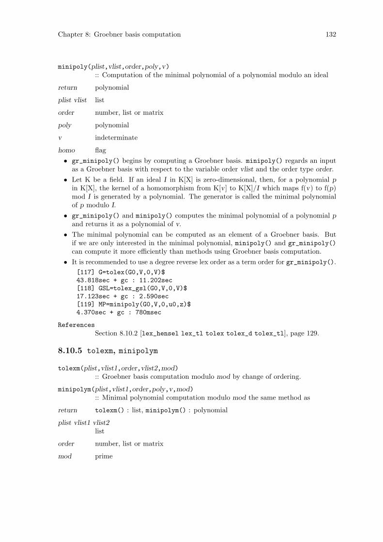
Chapter 8: Groebner basis computation 132
minipoly(plist,vlist,order,poly,v):: Computation of the minimal polynomial of a polynomial modulo an ideal
return polynomial
plist vlist list
order number, list or matrix
poly polynomial
v indeterminate
homo flag
• gr_minipoly() begins by computing a Groebner basis. minipoly() regards an inputas a Groebner basis with respect to the variable order vlist and the order type order.
• Let K be a field. If an ideal I in K[X] is zero-dimensional, then, for a polynomial pin K[X], the kernel of a homomorphism from K[v ] to K[X]/I which maps f(v) to f(p)mod I is generated by a polynomial. The generator is called the minimal polynomialof p modulo I.
• gr_minipoly() and minipoly() computes the minimal polynomial of a polynomial pand returns it as a polynomial of v.
• The minimal polynomial can be computed as an element of a Groebner basis. Butif we are only interested in the minimal polynomial, minipoly() and gr_minipoly()
can compute it more efficiently than methods using Groebner basis computation.
• It is recommended to use a degree reverse lex order as a term order for gr_minipoly().
[117] G=tolex(G0,V,0,V)$43.818sec + gc : 11.202sec[118] GSL=tolex_gsl(G0,V,0,V)$17.123sec + gc : 2.590sec[119] MP=minipoly(G0,V,0,u0,z)$4.370sec + gc : 780msec
References
Section 8.10.2 [lex_hensel lex_tl tolex tolex_d tolex_tl], page 129.
8.10.5 tolexm, minipolym
tolexm(plist,vlist1,order,vlist2,mod):: Groebner basis computation modulo mod by change of ordering.
minipolym(plist,vlist1,order,poly,v,mod):: Minimal polynomial computation modulo mod the same method as
return tolexm() : list, minipolym() : polynomial
plist vlist1 vlist2list
order number, list or matrix
mod prime

Chapter 8: Groebner basis computation 133
• An input plist must be a Groebner basis modulo mod with respect to the variable ordervlist1 and the order type order.
• minipolym() executes the same computation as in minipoly.
• tolexm() computes a lex order Groebner basis modulomod with respect to the variableorder vlist2, by using FGLM algorithm.
[197] tolexm(G0,V,0,V,31991);[8271*u0^31+10435*u0^30+816*u0^29+26809*u0^28+...,...][198] minipolym(G0,V,0,u0,z,31991);z^32+11405*z^31+20868*z^30+21602*z^29+...
References
Section 8.10.2 [lex_hensel lex_tl tolex tolex_d tolex_tl], page 129, Sec-tion 8.10.4 [gr_minipoly minipoly], page 131.
8.10.6 dp_gr_main, dp_gr_mod_main, dp_gr_f_main, dp_weyl_gr_main,dp_weyl_gr_mod_main, dp_weyl_gr_f_main
dp_gr_main(plist,vlist,homo,modular,order)dp_gr_mod_main(plist,vlist,homo,modular,order)dp_gr_f_main(plist,vlist,homo,order)dp_weyl_gr_main(plist,vlist,homo,modular,order)dp_weyl_gr_mod_main(plist,vlist,homo,modular,order)dp_weyl_gr_f_main(plist,vlist,homo,order)
:: Groebner basis computation (built-in functions)
return list
plist vlist list
order number, list or matrix
homo flag
modular flag or prime
• These functions are fundamental built-in functions for Groebner basis computation andgr(),hgr() and gr_mod() are all interfaces to these functions. Functions whose namescontain weyl are those for computation in Weyl algebra.
• dp_gr_f_main() and dp_weyl_gr_f_main() are functions for Groebner basis compu-tation over various finite fields. Coefficients of input polynomials must be converted toelements of a finite field currently specified by setmod_ff().
• If homo is not equal to 0, homogenization is applied before entering Buchberger algo-rithm
• For dp_gr_mod_main(), modular means a computation over GF(modular). For dp_
gr_main(), modular has the following mean.
1. If modular is 1 , trace lifting is used. Primes for trace lifting are generated bylprime(), starting from lprime(0), until the computation succeeds.
2. If modular is an integer greater than 1, the integer is regarded as a prime and tracelifting is executed by using the prime. If the computation fails then 0 is returned.

Chapter 8: Groebner basis computation 134
3. If modular is negative, the above rule is applied for -modular but the Groebnerbasis check and ideal-membership check are omitted in the last stage of tracelifting.
• gr(P,V,O), hgr(P,V,O) and gr_mod(P,V,O,M) execute dp_gr_main(P,V,0,1,O), dp_gr_main(P,V,1,1,O) and dp_gr_mod_main(P,V,0,M,O) respectively.
• Actual computation is controlled by various parameters set by dp_gr_flags(), otherthen by homo and modular.
References
Section 8.10.10 [dp_ord], page 136, Section 8.10.9 [dp_gr_flags dp_gr_print],page 135, Section 8.10.1 [gr hgr gr_mod], page 128, Section 10.5.1 [setmod_ff],page 167, Section 8.4 [Controlling Groebner basis computations], page 120
8.10.7 dp_f4_main, dp_f4_mod_main, dp_weyl_f4_main, dp_weyl_f4_mod_main
dp_f4_main(plist,vlist,order)dp_f4_mod_main(plist,vlist,order)dp_weyl_f4_main(plist,vlist,order)dp_weyl_f4_mod_main(plist,vlist,order)
:: Groebner basis computation by F4 algorithm (built-in functions)
return list
plist vlist list
order number, list or matrix
• These functions compute Groebner bases by F4 algorithm.
• F4 is a new generation algorithm for Groebner basis computation invented by J.C.Faugere. The current implementation of dp_f4_main() uses Chinese Remainder theo-rem and not highly optimized.
• Arguments and actions are the same as those of dp_gr_main(), dp_gr_mod_main(),dp_weyl_gr_main(), dp_weyl_gr_mod_main(), except for lack of the argument forcontrolling homogenization.
References
Section 8.10.10 [dp_ord], page 136, Section 8.10.9 [dp_gr_flags dp_gr_print],page 135, Section 8.10.1 [gr hgr gr_mod], page 128, Section 8.4 [ControllingGroebner basis computations], page 120
8.10.8 nd_gr, nd_gr_trace, nd_f4, nd_f4_trace, nd_weyl_gr, nd_weyl_gr_trace
nd_gr(plist,vlist,p,order)nd_gr_trace(plist,vlist,homo,p,order)nd_f4(plist,vlist,modular,order)nd_f4_trace(plist,vlist,homo,p,order)
nd_weyl_gr(plist,vlist,p,order)nd_weyl_gr_trace(plist,vlist,homo,p,order)
:: Groebner basis computation (built-in functions)

Chapter 8: Groebner basis computation 135
return list
plist vlist list
order number, list or matrix
homo flag
modular flag or prime
• These functions are new implementations for computing Groebner bases.
• nd_gr executes Buchberger algorithm over the rationals if p is 0, and that over GF(p)if p is a prime.
• nd_gr_trace executes the trace algorithm over the rationals. If p is 0 or 1, the tracealgorithm is executed until it succeeds by using automatically chosen primes. If pa positive prime, the trace is comuted over GF(p). If the trace algorithm fails 0 isreturned. If p is negative, the Groebner basis check and ideal-membership check areomitted. In this case, an automatically chosen prime if p is 1, otherwise the specifiedprime is used to compute a Groebner basis candidate. Execution of nd_f4_trace isdone as follows: For each total degree, an F4-reduction of S-polynomials over a finitefield is done, and S-polynomials which give non-zero basis elements are gathered. ThenF4-reduction over Q is done for the gathered S-polynomials. The obtained polynomialset is a Groebner basis candidate and the same check procedure as in the case ofnd_gr_trace is done.
• nd_f4 executes F4 algorithm over Q if modular is equal to 0, or over a finite fieldGF(modular) if modular is a prime number of machine size (<2^29).
• nd_weyl_gr, nd_weyl_gr_trace are for Weyl algebra computation.
• Each function cannot handle rational function coefficient cases.
• In general these functions are more efficient than dp_gr_main, dp_gr_mod_main, espe-cially over finite fields.
[38] load("cyclic")$[49] C=cyclic(7)$[50] V=vars(C)$[51] cputime(1)$[52] dp_gr_mod_main(C,V,0,31991,0)$26.06sec + gc : 0.313sec(26.4sec)[53] nd_gr(C,V,31991,0)$ndv_alloc=14771885.737sec + gc : 0.1837sec(5.921sec)[54] dp_f4_mod_main(C,V,31991,0)$3.51sec + gc : 0.7109sec(4.221sec)[55] nd_f4(C,V,31991,0)$1.906sec + gc : 0.126sec(2.032sec)
References
Section 8.10.10 [dp_ord], page 136, Section 8.10.9 [dp_gr_flags dp_gr_print],page 135, Section 8.4 [Controlling Groebner basis computations], page 120
8.10.9 dp_gr_flags, dp_gr_print

Chapter 8: Groebner basis computation 136
dp_gr_flags([list])dp_gr_print([i])
and showing informations.
return value currently set
list list
i integer
• dp_gr_flags() sets and shows various parameters for Groebner basis computation.
• If no argument is specified the current settings are returned.
• Arguments must be specified as a list such as ["Print",1,"NoSugar",1,...]. Namesof parameters must be character strings.
• dp_gr_print() is used to set and show the value of a parameter Print and PrintShort.
i=0 Print=0, PrintShort=0
i=1 Print=1, PrintShort=0
i=2 Print=0, PrintShort=1
This functions is prepared to get quickly the value when a user defined function callingdp_gr_main() etc. uses the value as a flag for showing intermediate informations.
References
Section 8.4 [Controlling Groebner basis computations], page 120
8.10.10 dp_ord
dp_ord([order]):: Set and show the ordering type.
return ordering type (number, list or matrix)
order number, list or matrix
• If an argument is specified, the function sets the current ordering type to order. If noargument is specified, the function returns the ordering type currently set.
• There are two types of functions concerning distributed polynomial, functions whichtake a ordering type and those which don’t take it. The latter ones use the currentsetting.
• Functions such as gr(), which need a ordering type as an argument, call dp_ord()internally during the execution. The setting remains after the execution.
Fundamental arithmetics for distributed polynomial also use the current setting. There-fore, when such arithmetics for distributed polynomials are done, the current settingmust coincide with the ordering type which was used upon the creation of the poly-nomials. It is assumed that such polynomials were generated under the same orderingtype.
• Type of term ordering must be correctly set by this function when functions other thantop level functions are called directly.

Chapter 8: Groebner basis computation 137
[19] dp_ord(0)$[20] <<1,2,3>>+<<3,1,1>>;(1)*<<1,2,3>>+(1)*<<3,1,1>>[21] dp_ord(2)$[22] <<1,2,3>>+<<3,1,1>>;(1)*<<3,1,1>>+(1)*<<1,2,3>>
References
Section 8.5 [Setting term orderings], page 123
8.10.11 dp_ptod
dp_ptod(poly,vlist):: Converts an ordinary polynomial into a distributed polynomial.
return distributed polynomial
poly polynomial
vlist list
• According to the variable ordering vlist and current type of term ordering, this functionconverts an ordinary polynomial into a distributed polynomial.
• Indeterminates not included in vlist are regarded to belong to the coefficient field.
[50] dp_ord(0);1[51] dp_ptod((x+y+z)^2,[x,y,z]);(1)*<<2,0,0>>+(2)*<<1,1,0>>+(1)*<<0,2,0>>+(2)*<<1,0,1>>+(2)*<<0,1,1>>+(1)*<<0,0,2>>[52] dp_ptod((x+y+z)^2,[x,y]);(1)*<<2,0>>+(2)*<<1,1>>+(1)*<<0,2>>+(2*z)*<<1,0>>+(2*z)*<<0,1>>+(z^2)*<<0,0>>
References
Section 8.10.12 [dp_dtop], page 137, Section 8.10.10 [dp_ord], page 136.
8.10.12 dp_dtop
dp_dtop(dpoly,vlist):: Converts a distributed polynomial into an ordinary polynomial.
return polynomial
dpoly distributed polynomial
vlist list
• This function converts a distributed polynomial into an ordinary polynomial accordingto a list of indeterminates vlist.
• vlist is such a list that its length coincides with the number of variables of dpoly.
[53] T=dp_ptod((x+y+z)^2,[x,y]);(1)*<<2,0>>+(2)*<<1,1>>+(1)*<<0,2>>+(2*z)*<<1,0>>+(2*z)*<<0,1>>+(z^2)*<<0,0>>[54] P=dp_dtop(T,[a,b]);z^2+(2*a+2*b)*z+a^2+2*b*a+b^2
Chapter 8: Groebner basis computation 138
8.10.13 dp_mod, dp_rat
dp_mod(p,mod,subst):: Converts a disributed polynomial into one with coefficients in a finite field.
dp_rat(p):: Converts a distributed polynomial with coefficients in a finite field into onewith coefficients in the rationals.
return distributed polynomial
p distributed polynomial
mod prime
subst list
• dp_nf_mod() and dp_true_nf_mod() require distributed polynomials with coefficientsin a finite field as arguments. dp_mod() is used to convert distributed polynomialswith rational number coefficients into appropriate ones. Polynomials with coefficientsin a finite field cannot be used as inputs of operations with polynomials with rationalnumber coefficients. dp_rat() is used for such cases.
• The ground finite field must be set in advance by using setmod().
• subst is such a list as [[var,value],...]. This is valid when the ground field of theinput polynomial is a rational function field. var’s are variables in the ground field andthe list means that value is substituted for var before converting the coefficients intoelements of a finite field.
References
Section 8.10.16 [dp_nf dp_nf_mod dp_true_nf dp_true_nf_mod], page 139,Section 6.3.11 [subst psubst], page 50, Section 6.1.16 [setmod], page 42.
8.10.14 dp_homo, dp_dehomo
dp_homo(dpoly):: Homogenize a distributed polynomial
dp_dehomo(dpoly):: Dehomogenize a homogenious distributed polynomial
return distributed polynomial
dpoly distributed polynomial
• dp_homo() makes a copy of dpoly, extends the length of the exponent vector of eachterm t in the copy by 1, and sets the value of the newly appended component tod-deg(t), where d is the total degree of dpoly.
• dp_dehomo() make a copy of dpoly and removes the last component of each terms inthe copy.
• Appropriate term orderings must be set when the results are used as inputs of someoperations.
• These are used internally in hgr() etc.

Chapter 8: Groebner basis computation 139
[202] X=<<1,2,3>>+3*<<1,2,1>>;(1)*<<1,2,3>>+(3)*<<1,2,1>>[203] dp_homo(X);(1)*<<1,2,3,0>>+(3)*<<1,2,1,2>>[204] dp_dehomo(@);(1)*<<1,2,3>>+(3)*<<1,2,1>>
References
Section 8.10.1 [gr hgr gr_mod], page 128.
8.10.15 dp_ptozp, dp_prim
dp_ptozp(dpoly):: Converts a distributed polynomial poly with rational coefficients into anintegral distributed polynomial such that GCD of all its coefficients is 1.
dp_prim(dpoly):: Converts a distributed polynomial poly with rational function coefficientsinto an integral distributed polynomial such that polynomial GCD of all itscoefficients is 1.
return distributed polynomial
dpoly distributed polynomial
• dp_ptozp() executes the same operation as ptozp() for a distributed polynomial. Ifthe coefficients include polynomials, polynomial contents included in the coefficientsare not removed.
• dp_prim() removes polynomial contents.
[208] X=dp_ptod(3*(x-y)*(y-z)*(z-x),[x]);(-3*y+3*z)*<<2>>+(3*y^2-3*z^2)*<<1>>+(-3*z*y^2+3*z^2*y)*<<0>>[209] dp_ptozp(X);(-y+z)*<<2>>+(y^2-z^2)*<<1>>+(-z*y^2+z^2*y)*<<0>>[210] dp_prim(X);(1)*<<2>>+(-y-z)*<<1>>+(z*y)*<<0>>
References
Section 6.3.18 [ptozp], page 55.
8.10.16 dp_nf, dp_nf_mod, dp_true_nf, dp_true_nf_mod
dp_nf(indexlist,dpoly,dpolyarray,fullreduce)
dp_nf_mod(indexlist,dpoly,dpolyarray,fullreduce,mod):: Computes the normal form of a distributed polynomial. (The result may bemultiplied by a constant in the ground field.)
dp_true_nf(indexlist,dpoly,dpolyarray,fullreduce)
dp_true_nf_mod(indexlist,dpoly,dpolyarray,fullreduce,mod):: Computes the normal form of a distributed polynomial. (The true result isreturned in such a list as [numerator, denominator])
return dp_nf() : distributed polynomial, dp_true_nf() : list

Chapter 8: Groebner basis computation 140
indexlist list
dpoly distributed polynomial
dpolyarrayarray of distributed polynomial
fullreduce flag
mod prime
• Computes the normal form of a distributed polynomial.
• dp_nf_mod() and dp_true_nf_mod() require distributed polynomials with coefficientsin a finite field as arguments.
• The result of dp_nf() may be multiplied by a constant in the ground field in order tomake the result integral. The same is true for dp_nf_mod(), but it returns the truenormal form if the ground field is a finite field.
• dp_true_nf() and dp_true_nf_mod() return such a list as [nm,dn]. Here nm isa distributed polynomial whose coefficients are integral in the ground field, dn is anintegral element in the ground field and nm/dn is the true normal form.
• dpolyarray is a vector whose components are distributed polynomials and indexlist isa list of indices which is used for the normal form computation.
• When argument fullreduce has non-zero value, all terms are reduced. When it hasvalue 0, only the head term is reduced.
• As for the polynomials specified by indexlist, one specified by an index placed at thepreceding position has priority to be selected.
• In general, the result of the function may be different depending on indexlist. However,the result is unique for Groebner bases.
• These functions are useful when a fixed non-distributed polynomial set is used as a setof reducers to compute normal forms of many polynomials. For single computationp_nf and p_true_nf are sufficient.
[0] load("gr")$[64] load("katsura")$[69] K=katsura(4)$[70] dp_ord(2)$[71] V=[u0,u1,u2,u3,u4]$[72] DP1=newvect(length(K),map(dp_ptod,K,V))$[73] G=gr(K,V,2)$[74] DP2=newvect(length(G),map(dp_ptod,G,V))$[75] T=dp_ptod((u0-u1+u2-u3+u4)^2,V)$[76] dp_dtop(dp_nf([0,1,2,3,4],T,DP1,1),V);u4^2+(6*u3+2*u2+6*u1-2)*u4+9*u3^2+(6*u2+18*u1-6)*u3+u2^2+(6*u1-2)*u2+9*u1^2-6*u1+1[77] dp_dtop(dp_nf([4,3,2,1,0],T,DP1,1),V);-5*u4^2+(-4*u3-4*u2-4*u1)*u4-u3^2-3*u3-u2^2+(2*u1-1)*u2-2*u1^2-3*u1+1[78] dp_dtop(dp_nf([0,1,2,3,4],T,DP2,1),V);-11380879768451657780886122972730785203470970010204714556333530492210456775930005716505560062087150928400876150217079820311439477560587583488*u4^15+...

Chapter 8: Groebner basis computation 141
[79] dp_dtop(dp_nf([4,3,2,1,0],T,DP2,1),V);-11380879768451657780886122972730785203470970010204714556333530492210456775930005716505560062087150928400876150217079820311439477560587583488*u4^15+...[80] @78==@79;1
References
Section 8.10.12 [dp_dtop], page 137, Section 8.10.10 [dp_ord], page 136, Sec-tion 8.10.13 [dp_mod dp_rat], page 138, Section 8.10.27 [p_nf p_nf_mod p_
true_nf p_true_nf_mod], page 146.
8.10.17 dp_hm, dp_ht, dp_hc, dp_rest
dp_hm(dpoly):: Gets the head monomial.
dp_ht(dpoly):: Gets the head term.
dp_hc(dpoly):: Gets the head coefficient.
dp_rest(dpoly):: Gets the remainder of the polynomial where the head monomial is removed.
return dp_hm(), dp_ht(), dp_rest() : distributed polynomial dp_hc() : number orpolynomial
dpoly distributed polynomial
• These are used to get various parts of a distributed polynomial.
• The next equations hold for a distributed polynomial p.
p = dp_hm(p) + dp_rest(p)
dp_hm(p) = dp_hc(p) dp_ht(p)[87] dp_ord(0)$[88] X=ptozp((a46^2+7/10*a46+7/48)*u3^4-50/27*a46^2-35/27*a46-49/216)$[89] T=dp_ptod(X,[u3,u4,a46])$[90] dp_hm(T);(2160)*<<4,0,2>>[91] dp_ht(T);(1)*<<4,0,2>>[92] dp_hc(T);2160[93] dp_rest(T);(1512)*<<4,0,1>>+(315)*<<4,0,0>>+(-4000)*<<0,0,2>>+(-2800)*<<0,0,1>>+(-490)*<<0,0,0>>
8.10.18 dp_td, dp_sugar
dp_td(dpoly):: Gets the total degree of the head term.

Chapter 8: Groebner basis computation 142
dp_sugar(dpoly):: Gets the sugar of a polynomial.
return non-negative integer
dpoly distributed polynomial
onoff flag
• Function dp_td() returns the total degree of the head term, i.e., the sum of all exponentof variables in that term.
• Upon creation of a distributed polynomial, an integer called sugar is associated. Thisvalue is the total degree of the virtually homogenized one of the original polynomial.
• The quantity sugar is an important guide to determine the selection strategy of criticalpairs in Groebner basis computation.
[74] dp_ord(0)$[75] X=<<1,2>>+<<0,1>>$[76] Y=<<1,2>>+<<1,0>>$[77] Z=X-Y;(-1)*<<1,0>>+(1)*<<0,1>>[78] dp_sugar(T);3
8.10.19 dp_lcm
dp_lcm(dpoly1,dpoly2):: Returns the least common multiple of the head terms of the given two poly-nomials.
return distributed polynomial
dpoly1 dpoly2distributed polynomial
• Returns the least common multiple of the head terms of the given two polynomials,where coefficient is always set to 1.
[100] dp_lcm(<<1,2,3,4,5>>,<<5,4,3,2,1>>);(1)*<<5,4,3,4,5>>
References
Section 8.10.27 [p_nf p_nf_mod p_true_nf p_true_nf_mod], page 146.
8.10.20 dp_redble
dp_redble(dpoly1,dpoly2):: Checks whether one head term is divisible by the other head term.
return integer
dpoly1 dpoly2distributed polynomial
• Returns 1 if the head term of dpoly2 divides the head term of dpoly1; otherwise 0.

Chapter 8: Groebner basis computation 143
• Used for finding candidate terms at reduction of polynomials.
[148] C;(1)*<<1,1,1,0,0>>+(1)*<<0,1,1,1,0>>+(1)*<<1,1,0,0,1>>+(1)*<<1,0,0,1,1>>[149] T;(3)*<<2,1,0,0,0>>+(3)*<<1,2,0,0,0>>+(1)*<<0,3,0,0,0>>+(6)*<<1,1,1,0,0>>[150] for ( ; T; T = dp_rest(T)) print(dp_redble(T,C));0001
References
Section 8.10.25 [dp_red dp_red_mod], page 145.
8.10.21 dp_subd
dp_subd(dpoly1,dpoly2):: Returns the quotient monomial of the head terms.
return distributed polynomial
dpoly1 dpoly2distributed polynomial
• Gets dp_ht(dpoly1)/dp_ht(dpoly2). The coefficient of the result is always set to 1.
• Divisibility assumed.
[162] dp_subd(<<1,2,3,4,5>>,<<1,1,2,3,4>>);(1)*<<0,1,1,1,1>>
References
Section 8.10.25 [dp_red dp_red_mod], page 145.
8.10.22 dp_vtoe, dp_etov
dp_vtoe(vect):: Converts an exponent vector into a term.
dp_etov(dpoly):: Convert the head term of a distributed polynomial into an exponent vector.
return dp_vtoe : distributed polynomial, dp_etov : vector
vect vector
dpoly distributed polynomial
• dp_vtoe() generates a term whose exponent vector is vect.
• dp_etov() generates a vector which is the exponent vector of the head term of dpoly.
[211] X=<<1,2,3>>;(1)*<<1,2,3>>[212] V=dp_etov(X);[ 1 2 3 ][213] V[2]++$[214] Y=dp_vtoe(V);(1)*<<1,2,4>>

Chapter 8: Groebner basis computation 144
8.10.23 dp_mbase
dp_mbase(dplist):: Computes the monomial basis
return list of distributed polynomial
dplist list of distributed polynomial
• Assuming that dplist is a list of distributed polynomials which is a Groebner basis withrespect to the current ordering type and that the ideal I generated by dplist in K[X] iszero-dimensional, this function computes the monomial basis of a finite dimenstionalK-vector space K[X]/I.
• The number of elements in the monomial basis is equal to the K-dimenstion of K[X]/I.
[215] K=katsura(5)$[216] V=[u5,u4,u3,u2,u1,u0]$[217] G0=gr(K,V,0)$[218] H=map(dp_ptod,G0,V)$[219] map(dp_ptod,dp_mbase(H),V)$[u0^5,u4*u0^3,u3*u0^3,u2*u0^3,u1*u0^3,u0^4,u3^2*u0,u2*u3*u0,u1*u3*u0,u1*u2*u0,u1^2*u0,u4*u0^2,u3*u0^2,u2*u0^2,u1*u0^2,u0^3,u3^2,u2*u3,u1*u3,u1*u2,u1^2,u4*u0,u3*u0,u2*u0,u1*u0,u0^2,u4,u3,u2,u1,u0,1]
References
Section 8.10.1 [gr hgr gr_mod], page 128.
8.10.24 dp_mag
dp_mag(p):: Computes the sum of bit lengths of coefficients of a distributed polynomial.
return integer
p distributed polynomial
• This function computes the sum of bit lengths of coefficients of a distributed polynomialp. If a coefficient is non integral, the sum of bit lengths of the numerator and thedenominator is taken.
• This is a measure of the size of a polynomial. Especially for zero-dimensional systemcoefficient swells are often serious and the returned value is useful to detect such swells.
• If ShowMag and Print for dp_gr_flags() are on, values of dp_mag() for intermediatebasis elements are shown.
[221] X=dp_ptod((x+2*y)^10,[x,y])$[222] dp_mag(X);115
References
Section 8.10.9 [dp_gr_flags dp_gr_print], page 135.

Chapter 8: Groebner basis computation 145
8.10.25 dp_red, dp_red_mod
dp_red(dpoly1,dpoly2,dpoly3)
dp_red_mod(dpoly1,dpoly2,dpoly3,mod):: Single reduction operation
return list
dpoly1 dpoly2 dpoly3distributed polynomial
vlist list
mod prime
• Reduces a distributed polynomial, dpoly1 + dpoly2, by dpoly3 for single time.
• An input for dp_red_mod() must be converted into a distributed polynomial withcoefficients in a finite field.
• This implies that the divisibility of the head term of dpoly2 by the head term of dpoly3is assumed.
• When integral coefficients, computation is so carefully performed that no rational op-erations appear in the reduction procedure. It is computed for integers a and b, and aterm t as: a(dpoly1 + dpoly2)-bt dpoly3.
• The result is a list [a dpoly1,a dpoly2 - bt dpoly3].
[157] D=(3)*<<2,1,0,0,0>>+(3)*<<1,2,0,0,0>>+(1)*<<0,3,0,0,0>>;(3)*<<2,1,0,0,0>>+(3)*<<1,2,0,0,0>>+(1)*<<0,3,0,0,0>>[158] R=(6)*<<1,1,1,0,0>>;(6)*<<1,1,1,0,0>>[159] C=12*<<1,1,1,0,0>>+(1)*<<0,1,1,1,0>>+(1)*<<1,1,0,0,1>>;(12)*<<1,1,1,0,0>>+(1)*<<0,1,1,1,0>>+(1)*<<1,1,0,0,1>>[160] dp_red(D,R,C);[(6)*<<2,1,0,0,0>>+(6)*<<1,2,0,0,0>>+(2)*<<0,3,0,0,0>>,(-1)*<<0,1,1,1,0>>+(-1)*<<1,1,0,0,1>>]
References
Section 8.10.13 [dp_mod dp_rat], page 138.
8.10.26 dp_sp, dp_sp_mod
dp_sp(dpoly1,dpoly2)
dp_sp_mod(dpoly1,dpoly2,mod):: Computation of an S-polynomial
return distributed polynomial
dpoly1 dpoly2distributed polynomial
mod prime
• This function computes the S-polynomial of dpoly1 and dpoly2.
• Inputs of dp_sp_mod() must be polynomials with coefficients in a finite field.

Chapter 8: Groebner basis computation 146
• The result may be multiplied by a constant in the ground field in order to make theresult integral.
[227] X=dp_ptod(x^2*y+x*y,[x,y]);(1)*<<2,1>>+(1)*<<1,1>>[228] Y=dp_ptod(x*y^2+x*y,[x,y]);(1)*<<1,2>>+(1)*<<1,1>>[229] dp_sp(X,Y);(-1)*<<2,1>>+(1)*<<1,2>>
References
Section 8.10.13 [dp_mod dp_rat], page 138.
8.10.27 p_nf, p_nf_mod, p_true_nf, p_true_nf_mod
p_nf(poly,plist,vlist,order)p_nf_mod(poly,plist,vlist,order,mod)
:: Computes the normal form of the given polynomial. (The result may bemultiplied by a constant.)
p_true_nf(poly,plist,vlist,order)p_true_nf_mod(poly,plist,vlist,order,mod)
:: Computes the normal form of the given polynomial. (The result is returnedas a form of [numerator, denominator])
return p_nf : polynomial, p_true_nf : list
poly polynomial
plist vlist list
order number, list or matrix
mod prime
• Defined in the package ‘gr’.
• Obtains the normal form of a polynomial by a polynomial list.
• These are interfaces to dp_nf(), dp_true_nf(), dp_nf_mod(), dp_true_nf_mod
• The polynomial poly and the polynomials in plist is converted, according to the vari-able ordering vlist and type of term ordering otype, into their distributed polynomialcounterparts and passed to dp_nf().
• dp_nf(), dp_true_nf(), dp_nf_mod() and dp_true_nf_mod() is called with value 1for fullreduce.
• The result is converted back into an ordinary polynomial.
• As for p_true_nf(), p_true_nf_mod() refer to dp_true_nf() and dp_true_nf_mod().
[79] K = katsura(5)$[80] V = [u5,u4,u3,u2,u1,u0]$[81] G = hgr(K,V,2)$[82] p_nf(K[1],G,V,2);0[83] L = p_true_nf(K[1]+1,G,V,2);

Chapter 8: Groebner basis computation 147
[-1503...,-1503...][84] L[0]/L[1];1
References
Section 8.10.11 [dp_ptod], page 137, Section 8.10.12 [dp_dtop], page 137, Sec-tion 8.10.10 [dp_ord], page 136, Section 8.10.16 [dp_nf dp_nf_mod dp_true_nf
dp_true_nf_mod], page 139.
8.10.28 p_terms
p_terms(poly,vlist,order):: Monomials appearing in the given polynomial is collected into a list.
return list
poly polynomial
vlist list
order number, list or matrix
• Defined in the package ‘gr’.
• This returns a list which contains all non-zero monomials in the given polynomial. Themonomials are ordered according to the current type of term ordering and vlist.
• Since polynomials in a Groebner base often have very large coefficients, examining apolynomial as it is may sometimes be difficult to perform. For such a case, this functionenables to examine which term is really exists.
[233] G=gr(katsura(5),[u5,u4,u3,u2,u1,u0],2)$[234] p_terms(G[0],[u5,u4,u3,u2,u1,u0],2);[u5,u0^31,u0^30,u0^29,u0^28,u0^27,u0^26,u0^25,u0^24,u0^23,u0^22,u0^21,u0^20,u0^19,u0^18,u0^17,u0^16,u0^15,u0^14,u0^13,u0^12,u0^11,u0^10,u0^9,u0^8,u0^7,u0^6,u0^5,u0^4,u0^3,u0^2,u0,1]
8.10.29 gb_comp
gb_comp(plist1, plist2):: Checks whether two polynomial lists are equal or not as a set
return 0 or 1
plist1 plist2• This function checks whether plist1 and plist2 are equal or not as a set .
• For the same input and the same term ordering different functions for Groebner basiscomputations may produce different outputs as lists. This function compares such listswhether they are equal as a generating set of an ideal.
[243] C=cyclic(6)$[244] V=[c0,c1,c2,c3,c4,c5]$[245] G0=gr(C,V,0)$[246] G=tolex(G0,V,0,V)$[247] GG=lex_tl(C,V,0,V,0)$[248] gb_comp(G,GG);1

Chapter 8: Groebner basis computation 148
8.10.30 katsura, hkatsura, cyclic, hcyclic
katsura(n)
hkatsura(n)
cyclic(n)
hcyclic(n):: Generates a polynomial list of standard benchmark.
return list
n integer
• Function katsura() is defined in ‘katsura’, and function cyclic() in ‘cyclic’.
• These functions generate a series of polynomial sets, respectively, which are often usedfor testing and bench marking: katsura, cyclic and their homogenized versions.
• Polynomial set cyclic is sometimes called by other name: Arnborg, Lazard, andDavenport.
[74] load("katsura")$[79] load("cyclic")$[89] katsura(5);[u0+2*u4+2*u3+2*u2+2*u1+2*u5-1,2*u4*u0-u4+2*u1*u3+u2^2+2*u5*u1,2*u3*u0+2*u1*u4-u3+(2*u1+2*u5)*u2,2*u2*u0+2*u2*u4+(2*u1+2*u5)*u3-u2+u1^2,2*u1*u0+(2*u3+2*u5)*u4+2*u2*u3+2*u1*u2-u1,u0^2-u0+2*u4^2+2*u3^2+2*u2^2+2*u1^2+2*u5^2][90] hkatsura(5);[-t+u0+2*u4+2*u3+2*u2+2*u1+2*u5,-u4*t+2*u4*u0+2*u1*u3+u2^2+2*u5*u1,-u3*t+2*u3*u0+2*u1*u4+(2*u1+2*u5)*u2,-u2*t+2*u2*u0+2*u2*u4+(2*u1+2*u5)*u3+u1^2,-u1*t+2*u1*u0+(2*u3+2*u5)*u4+2*u2*u3+2*u1*u2,-u0*t+u0^2+2*u4^2+2*u3^2+2*u2^2+2*u1^2+2*u5^2][91] cyclic(6);[c5*c4*c3*c2*c1*c0-1,((((c4+c5)*c3+c5*c4)*c2+c5*c4*c3)*c1+c5*c4*c3*c2)*c0+c5*c4*c3*c2*c1,(((c3+c5)*c2+c5*c4)*c1+c5*c4*c3)*c0+c4*c3*c2*c1+c5*c4*c3*c2,((c2+c5)*c1+c5*c4)*c0+c3*c2*c1+c4*c3*c2+c5*c4*c3,(c1+c5)*c0+c2*c1+c3*c2+c4*c3+c5*c4,c0+c1+c2+c3+c4+c5][92] hcyclic(6);[-c^6+c5*c4*c3*c2*c1*c0,((((c4+c5)*c3+c5*c4)*c2+c5*c4*c3)*c1+c5*c4*c3*c2)*c0+c5*c4*c3*c2*c1,(((c3+c5)*c2+c5*c4)*c1+c5*c4*c3)*c0+c4*c3*c2*c1+c5*c4*c3*c2,((c2+c5)*c1+c5*c4)*c0+c3*c2*c1+c4*c3*c2+c5*c4*c3,(c1+c5)*c0+c2*c1+c3*c2+c4*c3+c5*c4,c0+c1+c2+c3+c4+c5]
References
Section 8.10.12 [dp_dtop], page 137.
8.10.31 primadec, primedec
primadec(plist,vlist)

Chapter 8: Groebner basis computation 149
primedec(plist,vlist):: Computes decompositions of ideals.
returnplist list of polynomials
vlist list of variables
• Function primadec() and primedec are defined in ‘primdec’.
• primadec(), primedec() are the function for primary ideal decomposition and primedecomposition of the radical over the rationals respectively.
• The arguments are a list of polynomials and a list of variables. These functions acceptideals with rational function coefficients only.
• primadec returns the list of pair lists consisting a primary component and its associatedprime.
• primedec returns the list of prime components.
• Each component is a Groebner basis and the corresponding term order is indicated bythe global variables PRIMAORD, PRIMEORD respectively.
• primadec implements the primary decompostion algorithm in [Shimoyama,Yokoyama].
• If one only wants to know the prime components of an ideal, then use primedec becauseprimadec may need additional costs if an input ideal is not radical.
[84] load("primdec")$[102] primedec([p*q*x-q^2*y^2+q^2*y,-p^2*x^2+p^2*x+p*q*y,(q^3*y^4-2*q^3*y^3+q^3*y^2)*x-q^3*y^4+q^3*y^3,-q^3*y^4+2*q^3*y^3+(-q^3+p*q^2)*y^2],[p,q,x,y]);[[y,x],[y,p],[x,q],[q,p],[x-1,q],[y-1,p],[(y-1)*x-y,q*y^2-2*q*y-p+q]][103] primadec([x,z*y,w*y^2,w^2*y-z^3,y^3],[x,y,z,w]);[[[x,z*y,y^2,w^2*y-z^3],[z,y,x]],[[w,x,z*y,z^3,y^3],[w,z,y,x]]]
References
Section 6.3.15 [fctr sqfr], page 52, Section 8.5 [Setting term orderings],page 123.
8.10.32 primedec_mod
primedec_mod(plist,vlist,ord,mod,strategy):: Computes decompositions of ideals over small finite fields.
returnplist list of polynomials
vlist list of variables
ord number, list or matrix
mod positive integer
strategy integer
• Function primedec_mod() is defined in ‘primdec_mod’ and implements the prime de-composition algorithm in [Yokoyama].

Chapter 8: Groebner basis computation 150
• primedec_mod() is the function for prime ideal decomposition of the radical of a poly-nomial ideal over small finite field, and they return a list of prime ideals, which areassociated primes of the input ideal.
• primedec_mod() gives the decomposition over GF(mod). The generators of each re-sulting component consists of integral polynomials.
• Each resulting component is a Groebner basis with respect to a term order specifiedby [vlist,ord].
• If strategy is non zero, then the early termination strategy is tried by computing theintersection of obtained components incrementally. In general, this strategy is usefulwhen the krull dimension of the ideal is high, but it may add some overhead if thedimension is small.
• If you want to see internal information during the computation, executedp_gr_print(2) in advance.
[0] load("primdec_mod")$[246] PP444=[x^8+x^2+t,y^8+y^2+t,z^8+z^2+t]$[247] primedec_mod(PP444,[x,y,z,t],0,2,1);[[y+z,x+z,z^8+z^2+t],[x+y,y^2+y+z^2+z+1,z^8+z^2+t],[y+z+1,x+z+1,z^8+z^2+t],[x+z,y^2+y+z^2+z+1,z^8+z^2+t],[y+z,x^2+x+z^2+z+1,z^8+z^2+t],[y+z+1,x^2+x+z^2+z+1,z^8+z^2+t],[x+z+1,y^2+y+z^2+z+1,z^8+z^2+t],[y+z+1,x+z,z^8+z^2+t],[x+y+1,y^2+y+z^2+z+1,z^8+z^2+t],[y+z,x+z+1,z^8+z^2+t]][248]
References
Section 6.3.17 [modfctr], page 54, Section 8.10.6 [dp_gr_main dp_
gr_mod_main dp_gr_f_main dp_weyl_gr_main dp_weyl_gr_mod_main
dp_weyl_gr_f_main], page 133, Section 8.5 [Setting term orderings],page 123, Section 8.10.9 [dp_gr_flags dp_gr_print], page 135.
8.10.33 bfunction, bfct, generic_bfct, ann, ann0
bfunction(f )bfct(f )generic_bfct(plist,vlist,dvlist,weight)
:: Computes the global b function of a polynomial or an ideal
ann(f )ann0(f ) :: Computes the annihilator of a power of polynomial
return polynomial or list
f polynomial
plist list of polynomials
vlist dvlistlist of variables
• These functions are defined in ‘bfct’.

Chapter 8: Groebner basis computation 151
• bfunction(f ) and bfct(f ) compute the global b-function b(s) of a polynomial f. b(s)is a polynomial of the minimal degree such that there exists P(x,s) in D[s], which is apolynomial ring over Weyl algebra D, and P(x,s)f^(s+1)=b(s)f^s holds.
• generic_bfct(f,vlist,dvlist,weight) computes the global b-function of a left ideal Iin D generated by plist, with respect to weight. vlist is the list of x-variables, vlist isthe list of corresponding D-variables.
• bfunction(f ) and bfct(f ) implement different algorithms and the efficiency dependson inputs.
• ann(f ) returns the generator set of the annihilator ideal of f ^s. ann(f ) returns a list[a,list], where a is the minimal integral root of the global b-function of f, and list isa list of polynomials obtained by substituting s in ann(f ) with a.
• See [Saito,Sturmfels,Takayama] for the details.
[0] load("bfct")$[216] bfunction(x^3+y^3+z^3+x^2*y^2*z^2+x*y*z);-9*s^5-63*s^4-173*s^3-233*s^2-154*s-40[217] fctr(@);[[-1,1],[s+2,1],[3*s+4,1],[3*s+5,1],[s+1,2]][218] F = [4*x^3*dt+y*z*dt+dx,x*z*dt+4*y^3*dt+dy,x*y*dt+5*z^4*dt+dz,-x^4-z*y*x-y^4-z^5+t]$[219] generic_bfct(F,[t,z,y,x],[dt,dz,dy,dx],[1,0,0,0]);20000*s^10-70000*s^9+101750*s^8-79375*s^7+35768*s^6-9277*s^5+1278*s^4-72*s^3[220] P=x^3-y^2$[221] ann(P);[2*dy*x+3*dx*y^2,-3*dx*x-2*dy*y+6*s][222] ann0(P);[-1,[2*dy*x+3*dx*y^2,-3*dx*x-2*dy*y-6]]
References
Section 8.9 [Weyl algebra], page 127.

Chapter 9: Algebraic numbers 152
9 Algebraic numbers
9.1 Representation of algebraic numbers
In Asir algebraic number fields are not defined as independent objects. Instead, individualalgebraic numbers are defined by some means. In Asir an algebraic number field is definedvirtually as a number field obtained by adjoining a finite number of algebraic numbers tothe rational number field.
A new algebraic number is introduced in Asir in such a way where it is defined as a rootof an uni-variate polynomial whose coefficients include already defined algebraic numbersas well as rational numbers. We shall call such a newly defined algebraic number a root.Also, we call such an uni-variate polynomial the defining polynomial of that root.
[0] A0=newalg(x^2+1);(#0)[1] A1=newalg(x^3+A0*x+A0);(#1)[2] [type(A0),ntype(A0)];[1,2]
In this example, the algebraic number assigned to A0 is defined as a root of a polynomialx^2+1; that of A1 is defined as a root of a polynomial x^3+A0*x+A0, which you see containsthe previously defined root (A0) in its coefficients.
The argument to newalg(), i.e., the defining polynomial, must satisfy the following condi-tions.
1. A defining polynomial must be an uni-variate polynomial.
2. A defining polynomial is used to simplify expressions containing that algebraic number.The procedure of such simplification is performed by an internal routine similar tothe built-in function srem(), where the defining polynomial is used for the secondargument, the divisor. By this reason, the leading coefficient of the defining polynomialmust be a rational number (must not be an algebraic number.)
3. Every coefficients of a defining polynomial must be a ‘(multi-variate) polynomial’ in al-ready defined root’s. Here, ‘(multi-variate) polynomial’ means a mathematical concept,not the object type ‘polynomial’ in Asir.
4. A defining polynomial must be irreducible over the field that is obtained by adjoiningall root’s contained in its coefficients to the rational number field.
Only the first two conditions (1 and 2) are checked by function newalg(). Among all,it should be emphasized that no check is done for the irreducibility at all. The reason isthat the irreducibility test requires enormously much computation time. You are trustedwhether to check it at your own risk.
Once a root has been defined by newalg() function, it is given the type identifier for anumber, and furthermore, the sub-type identifier for an algebraic number. (See Section 6.8.1[type], page 74, Section 6.8.2 [ntype], page 75.) Also, any rational combination of rationalnumbers and root’s is an algebraic number.
[87] N=(A0^2+A1)/(A1^2-A0-1);((#1+#0^2)/(#1^2-#0-1))

Chapter 9: Algebraic numbers 153
[88] [type(N),ntype(N)];[1,2]
As you see it in the example, a root is displayed as #n. But, you cannot input that root inits immediate output form. You have to refer to a root by a program variable assigned tothe root, or to get it by alg(n) function, or by several other indirect means. A strange useof newalg(), with a same argument polynomial (except for the name of its main variable),will yield the old root instead of a new root though it is apparently inefficient.
[90] alg(0);(#0)[91] newalg(t^2+1);(#0)
The defining polynomial of a root can be obtained by defpoly() function.
[96] defpoly(A0);t#0^2+1[97] defpoly(A1);t#1^3+t#0*t#1+t#0
Here, you see a strange expression, t#0 and t#1. They are a specially indeterminatesgenerated and maintained by Asir internally. Indeterminate t#0 corresponds to root #0, andt#0 to #1. These indeterminates also cannot be input directly by a user in their immediateforms. You can get them by several ways: by var() function, or algv(n) function.
[98] var(@);t#1[99] algv(0);t#0[100]
9.2 Operations over algebraic numbers
In the previous section, we explained about the representation of algebraic numbers andtheir defining method. Here, we describe operations on algebraic numbers. Only a fewfunctions are built-in, and almost all functions are provided as user defined functions. Thefile containing their definitions is ‘sp’, and it is placed under the same directory as ‘gr’ isplaced, i.e., the standard library directory of Asir.
[0] load("gr")$[1] load("sp")$
Or if you always need them, it is more convenient to include the load commands in‘$HOME/.asirrc’.
Like the other numbers, algebraic numbers can get arithmetic operations applied. Simplifi-cation, however, by defining polynomials are not automatically performed. It is left to usersto simplify their expressions. A fatal error shall result if the denominator expression will besimplified to 0. Therefore, be careful enough when you will create and deal with algebraicnumbers which may denominators in their expressions.
Use simpalg() function for simplification of algebraic numbers by defining polynomials.
[49] T=A0^2+1;(#0^2+1)

Chapter 9: Algebraic numbers 154
[50] simpalg(T);0
Function simpalg() simplifies algebraic numbers which have the same structures as rationalexpressions in their appearances.
[39] A0=newalg(x^2+1);(#0)[40] T=(A0^2+A0+1)/(A0+3);((#0^2+#0+1)/(#0+3))[41] simpalg(T);(3/10*#0+1/10)[42] T=1/(A0^2+1);((1)/(#0^2+1))[43] simpalg(T);div : division by 0stopped in invalgp at line 258 in file "/usr/local/lib/asir/sp"258 return 1/A;(debug)
This example shows an error caused by zero division in the course of program executionof simpalg(), which attempted to simplify an algebraic number expression of which thedenominator is 0.
Function simpalg() also can take a polynomial as its argument and simplifies algebraicnumbers in its coefficients.
[43] simpalg(1/A0*x+1/(A0+1));(-#0)*x+(-1/2*#0+1/2)
Thus, you can operate in polynomials which contain algebraic numbers as you do usually inordinary polynomials, except for proper simplification by simpalg(). You may sometimesfeel needs to convert root’s into indeterminates, especially when you are working for normcomputation in algorithms for algebraic factorization. Function algptorat() is used forsuch cases.
[83] A0=newalg(x^2+1);(#0)[84] A1=newalg(x^3+A0*x+A0);(#1)[85] T=(2*A0+A1*A0+A1^2)*x+(1+A1)/(2+A0);(#1^2+#0*#1+2*#0)*x+((#1+1)/(#0+2))[86] S=algptorat(T);(((t#0+2)*t#1^2+(t#0^2+2*t#0)*t#1+2*t#0^2+4*t#0)*x+t#1+1)/(t#0+2)[87] algptorat(coef(T,1));t#1^2+t#0*t#1+2*t#0
As you see by the example, function algptorat() converts root’s, #n, in polynomials andnumbers into its associated indeterminates, t#n. As was already mentioned those indeter-minates cannot be directly input in their immediate form. The restriction is adopted toavoid the confusion that might happen if the user could input such internally generatableindeterminates.
The associated indeterminate to a root is reversely converted into the root by rattoalgp()
function.

Chapter 9: Algebraic numbers 155
[88] rattoalgp(S,[alg(0)]);(((#0+2)/(#0+2))*t#1^2+((#0^2+2*#0)/(#0+2))*t#1+((2*#0^2+4*#0)/(#0+2)))*x+((1)/(#0+2))*t#1+((1)/(#0+2))[89] rattoalgp(S,[alg(0),alg(1)]);(((#0^3+6*#0^2+12*#0+8)*#1^2+(#0^4+6*#0^3+12*#0^2+8*#0)*#1+2*#0^4+12*#0^3+24*#0^2+16*#0)/(#0^3+6*#0^2+12*#0+8))*x+(((#0+2)*#1+#0+2)/(#0^2+4*#0+4))[90] rattoalgp(S,[alg(1),alg(0)]);(((#0+2)*#1^2+(#0^2+2*#0)*#1+2*#0^2+4*#0)/(#0+2))*x+((#1+1)/(#0+2))[91] simpalg(@89);(#1^2+#0*#1+2*#0)*x+((-1/5*#0+2/5)*#1-1/5*#0+2/5)[92] simpalg(@90);(#1^2+#0*#1+2*#0)*x+((-1/5*#0+2/5)*#1-1/5*#0+2/5)
Function rattoalgp() takes as the second argument a list consisting of root’s that you wantto convert, and converts them successively from the left. This example shows that apparentdifference of the results due to the order of such conversion will vanish by simplificationyielding the same result. Functions algptorat() and rattoalgp() can be convenientlyused for your own simplification.
9.3 Representation of algebraic numbers by distributedpolynomials
Simplification of algebraic numbers containing root is not done automatically and should bedone by users. There is another representation of algebraic numbers, for which the results offundamental operations are automatically simplified. This representations are designed sothat operations are efficiently performed especially when the field is a successive extensionand it can be used as a ground field for Groebner basis related functions. Internally analgebraic number of this type is defined as an object called DAlg. A DAlg is represented asa fraction. The denominator is an integer and the numerator is a distributed polynomialwith integral coefficients.
DAlg is generated as an element of an algebraic number field set by set_field(). Thereare two methods to generate a DAlg. algtodalg() converts an algebraic number containingroot to DAlg. dptodalg() directly converts a distributed polynomial to DAlg.
[0] A=newalg(x^2+1);(#0)[1] B=newalg(x^3+A*x+A);(#1)[2] set_field([B,A]);0[3] C=algtodalg(A+B);((1)*<<1,0>>+(1)*<<0,1>>)[4] C^5;((-11)*<<2,1>>+(5)*<<2,0>>+(10)*<<1,1>>+(9)*<<1,0>>+(11)*<<0,1>>+(-1)*<<0,0>>)[5] 1/C;((2)*<<2,1>>+(-1)*<<2,0>>+(1)*<<1,1>>+(2)*<<1,0>>+(-3)*<<0,1>>

Chapter 9: Algebraic numbers 156
+(-1)*<<0,0>>)/5
In this example Q(a,b) (a^2+1=0, b^3+ab+b=0) is set as the current ground field, and(a+b)^5 and 1/(a+b) are simplified in the field. The numerators of the results are printedas distributed polynomials.
9.4 Operations for uni-variate polynomials over an algebraicnumber field
In the file ‘sp’ are provided functions for uni-variate polynomial factorization and uni-variatepolynomial GCD computation over algebraic numbers, and furthermore, as an applicationof them, functions to compute splitting fields of univariate polynomials.
9.4.1 GCD
Greatest common divisors (GCD) over algebraic number fields are computed by cr_gcda()
function. This function computes GCD by using modular computation and Chinese re-mainder theorem and it works for the case where the ground field is a multiple extension.
[63] A=newalg(t^9-15*t^6-87*t^3-125);(#0)[64] B=newalg(75*s^2+(10*A^7-175*A^4-470*A)*s+3*A^8-45*A^5-261*A^2);(#1)[65] P1=75*x^2+(150*B+10*A^7-175*A^4-395*A)*x+(75*B^2+(10*A^7-175*A^4-395*A)*B+13*A^8-220*A^5-581*A^2)$[66] P2=x^2+A*x+A^2$[67] cr_gcda(P1,P2);27*x+((#0^6-19*#0^3-65)*#1-#0^7+19*#0^4+38*#0)
9.4.2 Square-free factorization and Factorization
For square-free factorization (of uni-variate polynomials over algebraic number fields), weemploy the most fundamental algorithm which begins first to compute GCD of a polynomialand its derivative. The function to do this factorization is asq().
[116] A=newalg(x^2+x+1);(#4)[117] T=simpalg((x+A+1)*(x^2-2*A-3)^2*(x^3-x-A)^2);x^11+(#4+1)*x^10+(-4*#4-8)*x^9+(-10*#4-4)*x^8+(16*#4+20)*x^7+(24*#4-6)*x^6+(-29*#4-31)*x^5+(-15*#4+28)*x^4+(38*#4+29)*x^3+(#4-23)*x^2+(-21*#4-7)*x+(3*#4+8)[118] asq(T);[[x^5+(-2*#4-4)*x^3+(-#4)*x^2+(2*#4+3)*x+(#4-2),2],[x+(#4+1),1]]
Like factorization over the rational number field, the result is presented, commonly to bothsquare-free factorization and factorization, as a list whose elements are pairs (list of twoelements) in the form [factor, multiplicity] without the constant multiple part.
Here, it should be noticed that the products of all factors of the result may DIFFERfrom the input polynomial by a constant. The reason is that the factors are normalized sothat they have integral leading coefficients for the sake of readability.
This incongruity may happen to square-free factorization and factorization commonly.

Chapter 9: Algebraic numbers 157
The algorithm employed for factorization over algebraic number fields is an improvementof the norm method by Trager. It is especially very effective to factorize a polynomial overa field obtained by adjoining some of its root’s to the base field.
[119] af(T,[A]);[[x^3-x+(-#4),2],[x^2+(-2*#4-3),2],[x+(#4+1),1]]
The function takes two arguments: The second argument is a list of root’s. Factorizationis performed over a field obtained by adjoining the root’s to the rational number field. Itis important to keep in mind that the ordering of the root’s must obey a restriction: Lastdefined should come first. The automatic re-ordering is not done. It should be done byyourself.
The efficiency of factorization via norm depends on the efficiency of the norm computationand univariate factorization over the rationals. Especially the latter often causes combina-torial explosion and the computation will stick in such a case.
[120] B=newalg(x^2-2*A-3);(#5)[121] af(T,[B,A]);[[x+(#5),2],[x^3-x+(-#4),2],[x+(-#5),2],[x+(#4+1),1]]
9.4.3 Splitting fields
This operation may be somewhat unusual and for specific interest. (Galois Group forexample.) Procedurally, however, it is easy to obtain the splitting field of a polynomialby repeated application of algebraic factorization described in the previous section. Thefunction is sp().
[103] sp(x^5-2);[[x+(-#1),2*x+(#0^3*#1^3+#0^4*#1^2+2*#1+2*#0),2*x+(-#0^4*#1^2),2*x+(-#0^3*#1^3),x+(-#0)],[[(#1),t#1^4+t#0*t#1^3+t#0^2*t#1^2+t#0^3*t#1+t#0^4],[(#0),t#0^5-2]]]
Function sp() takes only one argument. The result is a list of two element: The first elementis a list of linear factors, and the second one is a list whose elements are pairs (list of twoelements) in the form [root, algptorat(defining polynomial)]. The second element, a listof pairs of form [root,algptorat(defining polynomial)], corresponds to the root’s whichare adjoined to eventually obtain the splitting field. They are listed in the reverse orderof adjoining. Each of the defining polynomials in the list is, of course, guaranteed to beirreducible over the field obtained by adjoining all root’s defined before it.
The first element of the result, a list of linear factors, contains all irreducible factors of theinput polynomial over the field obtained by adjoining all root’s in the second element of theresult. Because such field is the splitting field of the input polynomial, factors in the resultare all linear as the consequence.
Similarly to function af(), the product of all resulting factors may yield a polynomialwhich differs by a constant.
9.5 Summary of functions for algebraic numbers

Chapter 9: Algebraic numbers 158
9.5.1 newalg
newalg(defpoly):: Creates a new root.
return algebraic number (root)
defpoly polynomial
• Creates a new root (algebraic number) with its defining polynomial defpoly.
• For constraints on defpoly, See Section 9.1 [Representation of algebraic numbers],page 152.
[0] A0=newalg(x^2-2);(#0)
Reference
Section 9.5.2 [defpoly], page 158
9.5.2 defpoly
defpoly(alg):: Returns the defining polynomial of root alg.
return polynomial
alg algebraic number (root)
• Returns the defining polynomial of root alg.
• If the argument alg, a root, is #n, then the main variable of its defining polynomial ist#n.
[1] defpoly(A0);t#0^2-2
Reference
Section 9.5.1 [newalg], page 158, Section 9.5.3 [alg], page 158, Section 9.5.4[algv], page 159
9.5.3 alg
alg(i) :: Returns a root which correspond to the index i.
return algebraic number (root)
i integer
• Returns #i, a root.
• Because #i cannot be input directly, this function provides an alternative way: inputalg(i).
[2] x+#0;syntax error0[3] alg(0);(#0)
Reference
Section 9.5.1 [newalg], page 158, Section 9.5.4 [algv], page 159

Chapter 9: Algebraic numbers 159
9.5.4 algv
algv(i) :: Returns the associated indeterminate with alg(i).
return polynomial
i integer
• Returns an indeterminate t#i
• Since indeterminate t#i cannot be input directly, it is input by algv(i).
[4] var(defpoly(A0));t#0[5] t#0;syntax error0[6] algv(0);t#0
Reference
Section 9.5.1 [newalg], page 158, Section 9.5.2 [defpoly], page 158, Section 9.5.3[alg], page 158
9.5.5 simpalg
simpalg(rat):: Simplifies algebraic numbers in a rational expression.
return rational expression
rat rational expression
• Defined in the file ‘sp’.
• Simplifies algebraic numbers contained in numbers, polynomials, and rational expres-sions by the defining polynomials of root’s contained in them.
• If the argument is a number having the denominator, it is rationalized and the resultis a polynomial in root’s.
• If the argument is a polynomial, each coefficient is simplified.
• If the argument is a rational expression, its denominator and numerator are simplifiedas a polynomial.
[7] simpalg((1+A0)/(1-A0));simpalg undefinedreturn to toplevel[7] load("sp")$[46] simpalg((1+A0)/(1-A0));(-2*#0-3)[47] simpalg((2-A0)/(2+A0)*x^2-1/(3+A0));(-2*#0+3)*x^2+(1/7*#0-3/7)[48] simpalg((x+1/(A0-1))/(x-1/(A0+1)));(x+(#0+1))/(x+(-#0+1))

Chapter 9: Algebraic numbers 160
9.5.6 algptorat
algptorat(poly):: Substitutes the associated indeterminate for every root
return polynomial
poly polynomial
• Defined in the file ‘sp’.
• Substitutes the associated indeterminate t#n for every root #n in a polynomial.
[49] algptorat((-2*alg(0)+3)*x^2+(1/7*alg(0)-3/7));(-2*t#0+3)*x^2+1/7*t#0-3/7
Reference
Section 9.5.2 [defpoly], page 158, Section 9.5.4 [algv], page 159
9.5.7 rattoalgp
rattoalgp(poly,alglist):: Substitutes a root for the associated indeterminate with the root.
return polynomial
poly polynomial
alglist list
• Defined in the file ‘sp’.
• The second argument is a list of root’s. Function rattoalgp() substitutes a root forthe associated indeterminate of the root.
[51] rattoalgp((-2*algv(0)+3)*x^2+(1/7*algv(0)-3/7),[alg(0)]);(-2*#0+3)*x^2+(1/7*#0-3/7)
Reference
Section 9.5.3 [alg], page 158, Section 9.5.4 [algv], page 159
9.5.8 cr_gcda
cr_gcda(poly1,poly2):: GCD of two uni-variate polynomials over an algebraic number field.
return polynomial
poly1 poly2polynomial
• Defined in the file ‘sp’.
• Finds the GCD of two uni-variate polynomials.
[76] X=x^6+3*x^5+6*x^4+x^3-3*x^2+12*x+16$[77] Y=x^6+6*x^5+24*x^4+8*x^3-48*x^2+384*x+1024$[78] A=newalg(X);(#0)[79] cr_gcda(X,subst(Y,x,x+A));x+(-#0)

Chapter 9: Algebraic numbers 161
Reference
Section 8.10.1 [gr hgr gr_mod], page 128, Section 9.5.10 [asq af af_noalg],page 161
9.5.9 sp_norm
sp_norm(alg,var,poly,alglist):: Norm computation over an algebraic number field.
return polynomial
var The main variable of poly
poly univariate polynomial
alg root
alglist root list
• Defined in the file ‘sp’.
• Computes the norm of poly with respect to alg. Namely, if we write K = Q(alglist \{alg}), The function returns a product of all conjugates of poly, where the conjugateof polynomial poly is a polynomial in which the algebraic number alg is substitutedfor its conjugate over K.
• The result is a polynomial over K.
• The method of computation depends on the input. Currently direct computation ofresultant and Chinese remainder theorem are used but the selection is not necessarilyoptimal. By setting the global variable USE_RES to 1, the builtin function res() isalways used.
[0] load("sp")$[39] A0=newalg(x^2+1)$[40] A1=newalg(x^2+A0)$[41] sp_norm(A1,x,x^3+A0*x+A1,[A1,A0]);x^6+(2*#0)*x^4+(#0^2)*x^2+(#0)[42] sp_norm(A0,x,@@,[A0]);x^12+2*x^8+5*x^4+1
Reference
Section 6.3.14 [res], page 52, Section 9.5.10 [asq af af_noalg], page 161
9.5.10 asq, af, af_noalg
asq(poly) :: Square-free factorization of polynomial poly over an algebraic number field.
af(poly,alglist)af_noalg(poly,defpolylist)
:: Factorization of polynomial poly over an algebraic number field.
return list
poly polynomial
alglist root list

Chapter 9: Algebraic numbers 162
defpolylist root list of pairs of an indeterminate and a polynomial
• Both defined in the file ‘sp’.
• If the inputs contain no root’s, these functions run fast since they invoke functions overthe integers. In contrast to this, if the inputs contain root’s, they sometimes take along time, since cr_gcda() is invoked.
• Function af() requires the specification of base field, i.e., list of root’s for its secondargument.
• In the second argument alglist, root defined last must come first.
• In af(F,AL), AL denotes a list of roots and it represents an algebraic number field. InAL=[An,...,A1] each Ak should be defined as a root of a defining polynomial whosecoefficients are in Q(A(k+1),...,An).
[1] A1 = newalg(x^2+1);[2] A2 = newalg(x^2+A1);[3] A3 = newalg(x^2+A2*x+A1);[4] af(x^2+A2*x+A1,[A2,A1]);[[x^2+(#1)*x+(#0),1]]
To call sp_noalg, one should replace each algebraic number ai in poly with an inde-terminate vi. defpolylist is a list [[vn,dn(vn,...,v1)],...,[v1,d(v1)]]. In this expressiondi(vi,...,v1) is a defining polynomial of ai represented as a multivariate polynomial.
[1] af_noalg(x^2+a2*x+a1,[[a2,a2^2+a1],[a1,a1^2+1]]);[[x^2+a2*x+a1,1]]
• The result is a list, as a result of usual factorization, whose elements is of the form[factor, multiplicity]. In the result of af_noalg, algebraic numbers in f̌actor are replacedby the indeterminates according to defpolylist.
• The product of all factors with multiplicities counted may differ from the input poly-nomial by a constant.
[98] A = newalg(t^2-2);(#0)[99] asq(-x^4+6*x^3+(2*alg(0)-9)*x^2+(-6*alg(0))*x-2);[[-x^2+3*x+(#0),2]][100] af(-x^2+3*x+alg(0),[alg(0)]);[[x+(#0-1),1],[-x+(#0+2),1]][101] af_noalg(-x^2+3*x+a,[[a,x^2-2]]);[[x+a-1,1],[-x+a+2,1]]
Reference
Section 9.5.8 [cr_gcda], page 160, Section 6.3.15 [fctr sqfr], page 52
9.5.11 sp, sp_noalg
sp(poly)sp_noalg(poly)
:: Finds the splitting field of polynomial poly and splits.
return list
poly polynomial

Chapter 9: Algebraic numbers 163
• Defined in the file ‘sp’.
• Finds the splitting field of poly, an uni-variate polynomial over with rational coeffi-cients, and splits it into its linear factors over the field.
• The result consists of a two element list: The first element is the list of all linear factorsof poly ; the second element is a list which represents the successive extension of thefield. In the result of sp_noalg all the algebraic numbers are replaced by the specialindeterminate associated with it, that is t#i for #i. By this operation the result ofsp_noalg is a list containing only integral polynomials.
• The splitting field is represented as a list of pairs of form [root,
algptorat(defpoly(root))]. In more detail, the list is interpreted as arepresentation of successive extension obtained by adjoining root’s to the rationalnumber field. Adjoining is performed from the right root to the left.
• sp() invokes sp_norm() internally. Computation of norm is done by several methodsaccording to the situation but the algorithm selection is not always optimal and asimple resultant computation is often superior to the other methods. By setting theglobal variable USE_RES to 1, the builtin function res() is always used.
[101] L=sp(x^9-54);[[x+(-#2),-54*x+(#1^6*#2^4),54*x+(#1^6*#2^4+54*#2),54*x+(-#1^8*#2^2),-54*x+(#1^5*#2^5),54*x+(#1^5*#2^5+#1^8*#2^2),-54*x+(-#1^7*#2^3-54*#1),54*x+(-#1^7*#2^3),x+(-#1)],[[(#2),t#2^6+t#1^3*t#2^3+t#1^6],[(#1),t#1^9-54]]][102] for(I=0,M=1;I<9;I++)M*=L[0][I];[111] M=simpalg(M);-1338925209984*x^9+72301961339136[112] ptozp(M);-x^9+54
Reference
Section 9.5.10 [asq af af_noalg], page 161, Section 9.5.2 [defpoly], page 158,Section 9.5.6 [algptorat], page 160, Section 9.5.9 [sp_norm], page 161.
9.5.12 set_field
set_field(rootlist):: Set an algebraic number field as the currernt ground field.
return 0
rootlist A list of root
• set_field() sets an algebraic number field generated by root in rootlist over Q.
• You don’t care about the order of root in rootlist, because root are automaticallyordered internally.
[0] A=newalg(x^2+1);(#0)[1] B=newalg(x^3+A);(#1)[2] C=newalg(x^4+B);(#1)

Chapter 9: Algebraic numbers 164
[3] set_field([C,B,A]);0
Reference
Section 9.5.13 [algtodalg dalgtoalg dptodalg dalgtodp], page 164
9.5.13 algtodalg, dalgtoalg, dptodalg, dalgtodp
algtodalg(alg):: Converts an algebraic number alg to a DAlg.
dalgtoalg(dalg):: Converts a DAlg dalg to an algebraic number.
dptodalg(dp):: Converts an algebraic number alg to a DAlg.
dalgtodp(dalg):: Converts a DAlg dalg to an algebraic number.
return An algebraic number, a DAlg or a list [distributed polynomial,denominator]
alg an algebraic number containing root
dp a distributed polynomial over Q
• These functions are converters between DAlg and an algebraic number containing root,or a distributed polynomial.
• A ground field to which a DAlg belongs must be set by set_field() in advance.
• dalgtodp() returns a list containing the numerator (a distributed polynomial) and thedenominator (an integer).
• algtodalg(), dptodalg() return the simplified result.
[0] A=newalg(x^2+1);(#0)[1] B=newalg(x^3+A*x+A);(#1)[2] set_field([B,A]);0[3] C=algtodalg((A+B)^10);((408)*<<2,1>>+(103)*<<2,0>>+(-36)*<<1,1>>+(-446)*<<1,0>>+(-332)*<<0,1>>+(-218)*<<0,0>>)[4] dalgtoalg(C);((408*#0+103)*#1^2+(-36*#0-446)*#1-332*#0-218)[5] D=dptodalg(<<10,10>>/10+2*<<5,5>>+1/3*<<0,0>>);((-9)*<<2,1>>+(57)*<<2,0>>+(-63)*<<1,1>>+(-12)*<<1,0>>+(-60)*<<0,1>>+(1)*<<0,0>>)/30[6] dalgtodp(D);[(-9)*<<2,1>>+(57)*<<2,0>>+(-63)*<<1,1>>+(-12)*<<1,0>>+(-60)*<<0,1>>+(1)*<<0,0>>,30]
Reference
Section 9.5.12 [set_field], page 163

Chapter 10: Finite fields 165
10 Finite fields
10.1 Representation of finite fields
On Asir GF(p), GF(2^n), GF(p^n) can be defined, where GF(p) is a finite prime field ofcharateristic p, GF(2^n) is a finite field of characteristic 2 and GF(p^n) is a finite extensionof GF(p). These are all defined by setmod_ff().
[0] P=pari(nextprime,2^50);1125899906842679[1] setmod_ff(P);1125899906842679[2] field_type_ff();1[3] load("fff");1[4] F=defpoly_mod2(50);x^50+x^4+x^3+x^2+1[5] setmod_ff(F);x^50+x^4+x^3+x^2+1[6] field_type_ff();2[7] setmod_ff(x^3+x+1,1125899906842679);[1*x^3+1*x+1,1125899906842679][8] field_type_ff();3[9] setmod_ff(3,5);[3,x^5+2*x+1,x][10] field_type_ff();4
If p is a positive integer, setmod_ff(p) sets GF(p) as the current base field. If f is aunivariate polynomial of degree n, setmod_ff(f ) sets GF(2^n) as the current base field.GF(2^n) is represented as an algebraic extension of GF(2) with the defining polynomial fmod 2. Furthermore, finite extensions of prime finite fields can be defined. See Section 3.2[Types of numbers], page 13. In all cases the primality check of the argument is not doneand the caller is responsible for it.
Correctly speaking there is no actual object corresponding to a ’base field’. Settinga base field means that operations on elements of finite fields are done according to thearithmetics of the base field. Thus, if operands of an arithmetic operation are both rationalnumbers, then the result is also a rational number. However, if one of the operands is ina finite field, then the other is automatically regarded as in the same finite field and theoperation is done in the finite field.
A non zero element of a finite field belongs to the number and has object identifier 1.Its number identifier is 6 if the finite field is GF(p), 7 if it is GF(2^n).
There are several methods to input an element of a finite field. An element of GF(p)can be input by simp_ff().

Chapter 10: Finite fields 166
[0] P=pari(nextprime,2^50);1125899906842679[1] setmod_ff(P);1125899906842679[2] A=simp_ff(2^100);3025[3] ntype(@@);6
In the case of GF(2^n) the following methods are available.
[0] setmod_ff(x^50+x^4+x^3+x^2+1);x^50+x^4+x^3+x^2+1[1] A=@;(@)[2] ptogf2n(x^50+1);(@^50+1)[3] simp_ff(@@);(@^4+@^3+@^2)[4] ntogf2n(2^10-1);(@^9+@^8+@^7+@^6+@^5+@^4+@^3+@^2+@+1)
Elements of finite fields are numbers and one can apply field arithmetics to them. @ is agenerator of GF(2^n) over GF(2). See Section 3.2 [Types of numbers], page 13.
10.2 Univariate polynomials on finite fields
In ‘fff’ square-free factorization, DDF (distinct degree factorization), irreducible factoriza-tion and primality check are implemented for univariate polynomials over finite fields.
Factorizers return lists of [factor,multiplicity]. The factor part is monic and the infor-mation on the leading coefficient of the input polynomial is abandoned.
The algorithm used in square-free factorization is the most primitive one.
The irreducible factorization proceeds as follows.
1. DDF
2. Nullspace computation by Berlekamp algorithm
3. Root finding of minimal polynomials of bases of the nullspace
4. Separation of irreducible factors by the roots
10.3 Polynomials on small finite fields
Amultivariate polynomial over small finite field set by setmod_ff(p,n) can be factorizedby using a builtin function sffctr(). modfctr() also factorizes a polynomial over a finiteprime field. Internally, modfctr() creates a sufficiently large field extension of the specifiedground field, and it calls sffctr(), then it constructs irreducible factors over the groundfield from the factors returned by sffctr().

Chapter 10: Finite fields 167
10.4 Elliptic curves on finite fields
Several fundamental operations on elliptic curves over finite fields are provided as built-infunctions.
An elliptic curve is specified by a vector [a b] of length 2, where a, b are elements offinite fields. If the current base field is a prime field, then [a b] represents y^2=x^3+ax+b.If the current base field is a finite field of characteristic 2, then [a b] representsy^2+xy=x^3+ax^2+b.
Points on an elliptic curve together with the point at infinity forms an additive group.The addition, the subtraction and the additive inverse operation are provided as ecm_add_ff(), ecm_sub_ff() and ecm_chsgn_ff() respectively. Here the representation of pointsare as follows.
• 0 denotes the point at infinity.
• The other points are represented by vectors [x y z] of length 3 with non-zero z.
[x y z] represents a projective coordinate and it corresponds to [x/z y/z] in the affinecoordinate. To apply the above operations to a point [x y ], [x y 1] should be used insteadas an argument. The result of an operation is also represented by the projective coordinate.As the third coordinate is not always equal to 1, one has to divide the first and the scondcoordinate by the third one to obtain the affine coordinate.
10.5 Functions for Finite fields
10.5.1 setmod_ff
setmod_ff([p|defpoly2])setmod_ff([defpolyp,p])setmod_ff([p,n])
:: Sets/Gets the current base fields.
return number or polynomial
p prime
defpoly2 univariate polynomial irreducible over GF(2)
defpolyp univariate polynomial irreducible over GF(p)
n the extension degree
• If the argument is a non-negative integer p, GF(p) is set as the current base field.
• If the argument is a polynomial defpoly2, GF(2^deg(defpoly2 mod 2)) =GF(2)[t]/(defpoly2(t) mod2) is set as the current base field.
• If the arguments are a polynomial defpolyp and a prime p, GF(p^deg(defpolyp)) =GF(p)[t]/(defpolyp(t)) is set as the current base field.
• If the arguments are a prime p and an extension degree n, GF(p^n) is set as the currentbase field. p^n must be less than 2^29 and if p is greater than or equal to 2^14, thenn must be equal to 1.

Chapter 10: Finite fields 168
• If no argument is specified, the modulus indicating the current base field is returned. Ifthe current base field is GF(p), p is returned. If it is GF(2^n), the defining polynomial isreturned. If it is GF(p^n) defined by setmod_ff(defpoly,p), [defpolyp,p] is returned.If it is GF(p^n) defined by setmod_ff(p,n), [p,defpoly,prim elem] is returned. Here,defpoly is the defining polynomial of the n-th extension, and prim elem is the generatorof the multiplicative group of GF(p^n).
• Any irreducible univariate polynomial over GF(2) is available to set GF(2^n). Howeverthe use of defpoly_mod2() is recommended for efficiency.
[174] defpoly_mod2(100);x^100+x^15+1[175] setmod_ff(@@);x^100+x^15+1[176] setmod_ff();x^100+x^15+1[177] setmod_ff(x^4+x+1,547);[1*x^4+1*x+1,547][178] setmod_ff(2,5);[2,x^5+x^2+1,x]
References
Section 10.5.14 [defpoly_mod2], page 174
10.5.2 field_type_ff
field_type_ff()
:: Type of the current base field.
return integer
• Returns the type of the current base field.
• If no field is set, 0 is returned. If GF(p) is set, 1 is returned. If GF(2^n) is set, 2 isreturned.
[0] field_type_ff();0[1] setmod_ff(3);3[2] field_type_ff();1[3] setmod_ff(x^2+x+1);x^2+x+1[4] field_type_ff();2
References
Section 10.5.1 [setmod_ff], page 167
10.5.3 field_order_ff
field_order_ff()
:: Order of the current base field.

Chapter 10: Finite fields 169
return integer
• Returns the order of the current base field.
• q is returned if the current base field is GF(q).
[0] field_order_ff();field_order_ff : current_ff is not setreturn to toplevel[0] setmod_ff(3);3[1] field_order_ff();3[2] setmod_ff(x^2+x+1);x^2+x+1[3] field_order_ff();4
References
Section 10.5.1 [setmod_ff], page 167
10.5.4 characteristic_ff
characteristic_ff()
:: Characteristic of the current base field.
return integer
• Returns the characteristic of the current base field.
• p is returned if GF(p), where p is a prime, is set. 2 is returned if GF(2^n) is set.
[0] characteristic_ff();characteristic_ff : current_ff is not setreturn to toplevel[0] setmod_ff(3);3[1] characteristic_ff();3[2] setmod_ff(x^2+x+1);x^2+x+1[3] characteristic_ff();2
References
Section 10.5.1 [setmod_ff], page 167
10.5.5 extdeg_ff
extdeg_ff()
:: Extension degree of the current base field over the prime field.
return integer
• Returns the extension degree of the current base field over the prime field.
• 1 is returned if GF(p), where p is a prime, is set. n is returned if GF(2^n) is set.

Chapter 10: Finite fields 170
[0] extdeg_ff();extdeg_ff : current_ff is not setreturn to toplevel[0] setmod_ff(3);3[1] extdeg_ff();1[2] setmod_ff(x^2+x+1);x^2+x+1[3] extdeg_ff();2
References
Section 10.5.1 [setmod_ff], page 167
10.5.6 simp_ff
simp_ff(obj):: Converts numbers or coefficients of polynomials into elements in finite fields.
return number or polynomial
obj number or polynomial
• Converts numbers or coefficients of polynomials into elements in finite fields.
• It is used to convert integers or intrgral polynomials int elements of finite fields orpolynomials over finite fields.
• An element of a finite field may not have the reduced representation. In such case anapplication of simp_ff ensures that the output has the reduced representation. If asmall finite field is set as a ground field, an integer is projected the finite prime field,then it is embedded into the ground field. ptosfp() can be used for direct projectionto the ground field.
[0] simp_ff((x+1)^10);x^10+10*x^9+45*x^8+120*x^7+210*x^6+252*x^5+210*x^4+120*x^3+45*x^2+10*x+1[1] setmod_ff(3);3[2] simp_ff((x+1)^10);1*x^10+1*x^9+1*x+1[3] ntype(coef(@@,10));6[4] setmod_ff(2,3);[2,x^3+x+1,x][5] simp_ff(1);@_0[6] simp_ff(2);0[7] ptosfp(2);@_1

Chapter 10: Finite fields 171
References
Section 10.5.1 [setmod_ff], page 167, Section 10.5.8 [lmptop], page 171, Sec-tion 10.5.10 [gf2nton], page 172, Section 10.5.13 [ptosfp sfptop], page 174
10.5.7 random_ff
random_ff()
:: Random generation of an element of a finite field.
return element of a finite field
• Generates an element of the current base field randomly.
• The same random generator as in random(), lrandom() is used.
[0] random_ff();random_ff : current_ff is not setreturn to toplevel[0] setmod_ff(pari(nextprime,2^40));1099511627791[1] random_ff();561856154357[2] random_ff();45141628299
References
Section 10.5.1 [setmod_ff], page 167, Section 6.1.8 [random], page 37, Sec-tion 6.1.9 [lrandom], page 37
10.5.8 lmptop
lmptop(obj):: Converts the coefficients of a polynomial over GF(p) into integers.
return integral polynomial
obj polynomial over GF(p)
• Converts the coefficients of a polynomial over GF(p) into integers.
• An element of GF(p) is represented by a non-negative integer r less than p. Eachcoefficient of a polynomial is converted into an integer object whose value is r.
[0] setmod_ff(pari(nextprime,2^40));1099511627791[1] F=simp_ff((x-1)^10);1*x^10+1099511627781*x^9+45*x^8+1099511627671*x^7+210*x^6+1099511627539*x^5+210*x^4+1099511627671*x^3+45*x^2+1099511627781*x+1[2] setmod_ff(547);547[3] F=simp_ff((x-1)^10);1*x^10+537*x^9+45*x^8+427*x^7+210*x^6+295*x^5+210*x^4+427*x^3+45*x^2+537*x+1[4] lmptop(F);x^10+537*x^9+45*x^8+427*x^7+210*x^6+295*x^5+210*x^4+427*x^3

Chapter 10: Finite fields 172
+45*x^2+537*x+1[5] lmptop(coef(F,1));537[6] ntype(@@);0
References
Section 10.5.6 [simp_ff], page 170
10.5.9 ntogf2n
ntogf2n(m)
:: Converts a non-negative integer into an element of GF(2^n).
return element of GF(2^n)
m non-negative integer
• Let m be a non-negative integer. m has the binary representationm=m0+m1*2+...+mk*2^k. This function returns an element of GF(2^n) =GF(2)[t]/(g(t)), m0+m1*t+...+mk*t^k mod g(t).
• Apply simp_ff() to reduce the result.
[1] setmod_ff(x^30+x+1);x^30+x+1[2] N=ntogf2n(2^100);(@^100)[3] simp_ff(N);(@^13+@^12+@^11+@^10)
References
Section 10.5.10 [gf2nton], page 172
10.5.10 gf2nton
gf2nton(m)
:: Converts an element of GF(2^n) into a non-negative integer.
return non-negative integer
m element of GF(2^n)
• The inverse of gf2nton.
[1] setmod_ff(x^30+x+1);x^30+x+1[2] N=gf2nton(2^100);(@^100)[3] simp_ff(N);(@^13+@^12+@^11+@^10)[4] gf2nton(N);1267650600228229401496703205376[5] gf2nton(simp_ff(N));15360

Chapter 10: Finite fields 173
References
Section 10.5.10 [gf2nton], page 172
10.5.11 ptogf2n
ptogf2n(poly):: Converts a univariate polynomial into an element of GF(2^n).
return element of GF(2^n)
poly univariate polynomial
• Generates an element of GF(2^n) represented by poly. The coefficients are reducedmodulo 2. The output is equal to the result by substituting @ for the variable of poly.
[1] setmod_ff(x^30+x+1);x^30+x+1[2] ptogf2n(x^100);(@^100)
References
Section 10.5.12 [gf2ntop], page 173
10.5.12 gf2ntop
gf2ntop(m[,v]):: Converts an element of GF(2^n) into a polynomial.
return univariate polynomial
m an element of GF(2^n)
v indeterminate
• Returns a polynomial representing m.
• If v is used as the variable of the output. If v is not specified, the variable of theargument of the latest ptogf2n() call. The default variable is x.
[1] setmod_ff(x^30+x+1);x^30+x+1[2] N=simp_ff(gf2ntop(2^100));(@^13+@^12+@^11+@^10)[5] gf2ntop(N);[207] gf2ntop(N);x^13+x^12+x^11+x^10[208] gf2ntop(N,t);t^13+t^12+t^11+t^10
References
Section 10.5.11 [ptogf2n], page 173
Chapter 10: Finite fields 174
10.5.13 ptosfp, sfptop
ptosfp(p)sfptop(p)
:: Transformation to/from a small finite field
return polynomial
p polynomial
• ptosfp() converts coefficients of a polynomial to elements in a small finite fieldGF(p^n) set as a ground field. If a coefficient is already an element of the field, noconversion is done. If a coefficient is a positive integer, then its residue modulo p^nis expanded as p-adic integer, then p is substituted by x, finally the polynomial isconverted to its correspoding logarithmic representation with respect to the primitiveelement. For example, GF(3^5) is represented as F(3)[x]/(x^5+2*x+1), and eachelement of the field is represented as @ k by its exponent k with respect to theprimitive element x. 23 = 2*3^2+3+2 is represented as 2*x^2+x+2 and it is equivalentto x^17 modulo x^5+2*x+1. Therefore an integer 23 is conterted to @ 17.
• sfptop() is the inverse of ptosfp().
[196] setmod_ff(3,5);[3,x^5+2*x+1,x][197] A = ptosfp(23);@_17[198] 9*2+3+2;23[199] x^17-(2*x^2+x+2);x^17-2*x^2-x-2[200] sremm(@,x^5+2*x+1,3);0[201] sfptop(A);23
References
Section 10.5.1 [setmod_ff], page 167, Section 10.5.6 [simp_ff], page 170
10.5.14 defpoly_mod2
defpoly_mod2(d):: Generates an irreducible univariate polynomial over GF(2).
return univariate polynomial
d positive integer
• Defined in ‘fff’.
• An irreducible univariate polynomial of degree d is returned.
• If an irreducible trinomial x^d+x^m+1 exists, then the one with the smallest m is re-turned. Otherwise, an irreducible pentanomial x^d+x^m1+x^m2+x^m3+1 (m1>m2>m3is returned. m1, m2 and m3 are determined as follows: Fix m1 as small as possible.Then fix m2 as small as possible. Then fix m3 as small as possible.

Chapter 10: Finite fields 175
References
Section 10.5.1 [setmod_ff], page 167
10.5.15 sffctr
sffctr(poly):: Irreducible factorization over a small finite field.
return list
poly polynomial over a finite field
• Factorize poly into irreducible factors over a small finite field currently set.
• The result is a list [[f1,m1],[f2,m2],...], where fi is a monic irreducible factor and mi isits multiplicity.
[0] setmod_ff(2,10);[2,x^10+x^3+1,x][1] sffctr((z*y^3+z*y)*x^3+(y^5+y^3+z*y^2+z)*x^2+z^11*y*x+z^10*y^3+z^11);[[@_0,1],[@_0*z*y*x+@_0*y^3+@_0*z,1],[(@_0*y+@_0)*x+@_0*z^5,2]]
References
Section 10.5.1 [setmod_ff], page 167, Section 6.3.17 [modfctr], page 54
10.5.16 fctr_ff
fctr_ff(poly):: Irreducible univariate factorization over a finite field.
return list
poly univariate polynomial over a finite field
• Defined in ‘fff’.
• Factorize poly into irreducible factors over the current base field.
• The result is a list [[f1,m1],[f2,m2],...], where fi is a monic irreducible factor and mi isits multiplicity.
• The leading coefficient of poly is abandoned.
[178] setmod_ff(2^64-95);18446744073709551521[179] fctr_ff(x^5+x+1);[[1*x+14123390394564558010,1],[1*x+6782485570826905238,1],[1*x+15987612182027639793,1],[1*x^2+1*x+1,1]]
References
Section 10.5.1 [setmod_ff], page 167
10.5.17 irredcheck_ff
irredcheck_ff(poly):: Primality check of a univariate polynomial over a finite field.
return 0|1

Chapter 10: Finite fields 176
poly univariate polynomial over a finite field
• Defined in ‘fff’.
• Returns 1 if poly is irreducible over the current base field. Returns 0 otherwise.
[178] setmod_ff(2^64-95);18446744073709551521[179] ] F=x^10+random_ff();x^10+14687973587364016969[180] irredcheck_ff(F);1
References
Section 10.5.1 [setmod_ff], page 167
10.5.18 randpoly_ff
randpoly_ff(d,v):: Generation of a random univariate polynomial over a finite field.
return polynomial
d positive integer
v indeterminate
• Defined in ‘fff’.
• Generates a polynomial of v such that the degree is less than d and the coefficients arein the current base field. The coefficients are generated by random_ff().
[178] setmod_ff(2^64-95);18446744073709551521[179] ] F=x^10+random_ff();[180] randpoly_ff(3,x);17135261454578964298*x^2+4766826699653615429*x+18317369440429479651[181] randpoly_ff(3,x);7565988813172050604*x^2+7430075767279665339*x+4699662986224873544[182] randpoly_ff(3,x);10247781277095450395*x^2+10243690944992524936*x+4063829049268845492
References
Section 10.5.1 [setmod_ff], page 167, Section 10.5.7 [random_ff], page 171
10.5.19 ecm_add_ff, ecm_sub_ff, ecm_chsgn_ff
ecm_add_ff(p1,p2,ec)ecm_sub_ff(p1,p2,ec)ecm_chsgn_ff(p1)
:: Addition, Subtraction and additive inverse for points on an elliptic curve.
return vector or 0
p1 p2 vector of length 3 or 0
ec vector of length 2

Chapter 10: Finite fields 177
• Let p1, p2 be points on the elliptic curve represented by ec over the current base field.ecm add ff(p1,p2,ec), ecm sub ff(p1,p2,ec) and ecm chsgn ff(p1) returns p1+p2, p1-p2and -p1 respectively.
• If the current base field is a prime field of odd order, then ec representsy^2=x^3+ec[0]x+ec[1]. If the characteristic of the current base field is 2, then ecrepresents y^2+xy=x^3+ec[0]x^2+ec[1].
• The point at infinity is represented by 0.
• If an argument denoting a point is a vector of length 3, then it is the projective coor-dinate. In such a case the third coordinate must not be 0.
• If the result is a vector of length 3, then the third coordinate is not equal to 0 butnot necessarily 1. To get the result by the affine coordinate, the first and the secondcoordinates should be divided by the third coordinate.
• The check whether the arguments are on the curve is omitted.
[0] setmod_ff(1125899906842679)$[1] EC=newvect(2,[ptolmp(1),ptolmp(1)])$[2] Pt1=newvect(3,[1,-412127497938252,1])$[3] Pt2=newvect(3,[6,-252647084363045,1])$[4] Pt3=ecm_add_ff(Pt1,Pt2,EC);[ 560137044461222 184453736165476 125 ][5] F=y^2-(x^3+EC[0]*x+EC[1])$[6] subst(F,x,Pt3[0]/Pt3[2],y,Pt3[1]/Pt3[2]);0[7] ecm_add_ff(Pt3,ecm_chsgn_ff(Pt3),EC);0[8] D=ecm_sub_ff(Pt3,Pt2,EC);[ 886545905133065 119584559149586 886545905133065 ][9] D[0]/D[2]==Pt1[0]/Pt1[2];1[10] D[1]/D[2]==Pt1[1]/Pt1[2];1
References
Section 10.5.1 [setmod_ff], page 167

Appendix A: Appendix 178
Appendix A Appendix
A.1 Details of syntax
<expression>:‘(’<expression>‘)’<expression> <binary operator> <expression>‘+’ <expression>‘-’ <expression><left value><left value> <assignment operator> <expression><left value> ‘++’<left value> ‘--’‘++’ <left value>‘--’ <left value>‘!’ <expression><expression> ‘?’ <expression> ‘:’ <expression><function> ‘(’ <expr list> ‘)’<function> ‘(’ <expr list> ‘|’ <option list> ‘)’<string><exponent vector><atom><list>
(See Section 4.2.10 [various expressions], page 24.)
<left value>:<program variable> [‘[’<expression>‘]’]*
<binary operator>:‘+’ ‘-’ ‘*’ ‘/’ ‘%’ ‘^’(exponentiation)‘==’ ‘!=’ ‘<’ ‘>’ ‘<=’ ‘>=’ ‘&&’ ‘||’‘==’ ‘!=’ ‘<’ ‘>’ ‘<=’ ‘>=’ ‘&&’ ‘||’
<assignment operator>:‘=’ ‘+=’ ‘-=’ ‘*=’ ‘/=’ ‘%=’ ‘^=’
<expr list>:<empty><expression> [‘,’ <expression>]*
<option>:Character sequence beginning with an alphabetical letter ‘=’ <expr>
<option list>:<option><option> [‘,’ <option>]*
<list>:‘[’ <expr list> ‘]’
<program variable>:Sequence of alphabetical letters or numeric digits or _that begins with a capital alphabetical letter(X,Y,Japan etc.)

Appendix A: Appendix 179
(See Section 4.2.2 [variables and indeterminates], page 19.)
<function>:Sequence of alphabetical letters or numeric digits or _that begins with a small alphabetical letter(fctr,gcd etc.)
<atom>:<indeterminate><number>
<indeterminate>:Sequence of alphabetical letters or numeric digits or _that begin with a small alphabetical letter(a,bCD,c1_2 etc.)
(See Section 4.2.2 [variables and indeterminates], page 19.)
<number>:<rational number><floating point number><algebraic number><complex number>
(See Section 3.2 [Types of numbers], page 13.)
<rational number>:0, 1, -2, 3/4
<floating point number>:0.0, 1.2e10
<algebraic number>:newalg(x^2+1), alg(0)^2+1
(See Chapter 9 [Algebraic numbers], page 152.)
<complex number>:1+@i, 2.3*@i
<string>:character sequence enclosed by two ‘"’’s.
<exponent vector>:‘<<’ <expr list> ‘>>’
(See Chapter 8 [Groebner basis computation], page 118.)
<statement>:<expression> <terminator><compound statement>‘break’ <terminator>‘continue’ <terminator>‘return’ <terminator>‘return’ <expression> <terminator>‘if’ ‘(’ <expr list> ‘)’ <statement>‘if’ ‘(’ <expr list> ‘)’ <statement> ‘else’ <statement>‘for’ ‘(’ <expr list> ‘;’ <expr list> ‘;’ <expr list> ‘)’ <statement>‘do’ <statement> ‘while’ ‘(’ <expr list> ‘)’ <terminator>‘while’ ‘(’ <expr list> ‘)’ <statement>‘def’ <function> ‘(’ <expr list> ‘)’ ‘{’ <variable declaration> <stat list> ‘}’

Appendix A: Appendix 180
‘end(quit)’ <terminator>
(See Section 4.2.5 [statements], page 21.)
<terminator>:‘;’ ‘$’
<variable declaration>:[‘extern’ <program variable> [‘,’ <program variable>]* <terminator>]*
<compound statement>:‘{’ <stat list> ‘}’
<stat list>:[<statement>]*
A.2 Files of user defined functions
There are several files of user defined functions under the standard library directory.(‘/usr/local/lib/asir’ by default.) Here, we explain some of them.
‘fff’ Univariate factorizer over large finite fields (See Chapter 10 [Finite fields],page 165.)
‘gr’ Groebner basis package. (See Chapter 8 [Groebner basis computation],page 118.)
‘sp’ Operations over algebraic numbers and factorization, Splitting fields. (SeeChapter 9 [Algebraic numbers], page 152.)
‘alpi’‘bgk’‘cyclic’‘katsura’‘kimura’ Example polynomial sets for benchmarks of Groebner basis computation. (See
Section 8.10.30 [katsura hkatsura cyclic hcyclic], page 148.)
‘defs.h’ Macro definitions. (See Section 4.2.11 [preprocessor], page 25.)
‘fctrtest’Test program of factorization of integral polynomials. It includes ‘factor.tst’of REDUCE and several examples for large multiplicity factors. If this file isload()’ed, computation will begin immediately. You may use it as a first testwhether Asir at you hand runs correctly.
‘fctrdata’This contains example polynomials for factorization. It includes polynomialsused in ‘fctrtest’. Polynomials contained in vector Alg[] is for the algebraicfactorization af(). (See Section 9.5.10 [asq af af noalg], page 161.)
[45] load("sp")$[84] load("fctrdata")$[175] cputime(1)$0msec[176] Alg[5];x^9-15*x^6-87*x^3-125

Appendix A: Appendix 181
0msec[177] af(Alg[5],[newalg(Alg[5])]);[[1,1],[75*x^2+(10*#0^7-175*#0^4-470*#0)*x+(3*#0^8-45*#0^5-261*#0^2),1],[75*x^2+(-10*#0^7+175*#0^4+395*#0)*x+(3*#0^8-45*#0^5-261*#0^2),1],[25*x^2+(25*#0)*x+(#0^8-15*#0^5-87*#0^2),1],[x^2+(#0)*x+(#0^2),1],[x+(-#0),1]]3.600sec + gc : 1.040sec
‘ifplot’ Examples for plotting. (See Section 7.5.15 [ifplot conplot plot polarplot plo-tover], page 113.) Vector IS[] contains several famous algebraic curves. Vari-ables H, D, C, S contains something like the suits (Heart, Diamond, Club, andSpade) of cards.
‘num’ Examples of simple operations on numbers.
‘mat’ Examples of simple operations on matrices.
‘ratint’ Indefinite integration of rational functions. For this, files ‘sp’ and ‘gr’ is neces-sary. A function ratint() is defined. Its returns a rather complex result.
[0] load("gr")$[45] load("sp")$[84] load("ratint")$[102] ratint(x^6/(x^5+x+1),x);[1/2*x^2,[[(#2)*log(-140*x+(-2737*#2^2+552*#2-131)),161*t#2^3-23*t#2^2+15*t#2-1],[(#1)*log(-5*x+(-21*#1-4)),21*t#1^2+3*t#1+1]]]
In this example, indefinite integral of the rational function x^6/(x^5+x+1) iscomputed. The result is a list which comprises two elements: The first elementis the rational part of the integral; The second part is the logarithmic part ofthe integral. The logarithmic part is again a list which comprises finite numberof elements, each of which is of form [root*log(poly),defpoly]. This pairshould be interpreted to sum up the expression root*log(poly) through allroot’s root’s of the defpoly. Here, poly contains root, and substitution forroot is equally applied to poly. The logarithmic part in total is obtained byapplying such interpretation to all element pairs in the second element of theresult and then summing them up all.
‘primdec’ Primary ideal decomposition of polynomial ideals and prime compotision ofradicals over the rationals (see Section 8.10.31 [primadec primedec], page 148).
‘primdec_mod’Prime decomposition of radicals of polynomial ideals over finite fields (see Sec-tion 8.10.32 [primedec mod], page 149).
‘bfct’ Computation of b-function. (see Section 8.10.33 [bfunction bfct generic bfctann ann0], page 150).

Appendix A: Appendix 182
A.3 Input interfaces
A command line editing facility and a history substitution facility are built-in for DOS,Windows version of Asir. UNIX versions of Asir do not have such built-in facilites. Instead,the following input interfaces are prepared. This are also available from our ftp server. Asfor our ftp server See Section 1.3 [How to get Risa/Asir], page 2.
On Windows, ‘asirgui.exe’ has a copy and paste functionality different from Windowsconvention. Press the left button of the mouse and drag the mouse cursor on a text, thenthe text is selected and is highlighted. When the button is released, highlighted text returnsto the normal state and it is saved in the copy buffer. If the right button is pressed, thetext in the copy buffer is inserted at the current text cursor position. Note that the existingtext is read-only and one cannot modify it.
A.3.1 fep
Fep is a general purpose front end processor. The author is K. Utashiro (SRA Inc.).
Under fep, emacs- or vi-like command line editing and csh-like history substitution areavailable for UNIX commands, including ‘asir’.
% fep asir...[0] fctr(x^5-1);[[1,1],[x-1,1],[x^4+x^3+x^2+x+1,1]][1] !! /* !!+Return */fctr(x^5-1); /* The last input appears. */... /* Edit+Return */fctr(x^5+1);[[1,1],[x+1,1],[x^4-x^3+x^2-x+1,1]]
Fep is a free software and the source is available. However machines or operating systems onwhich the original one can run are limited. The modified version by us running on severalunsupported environments is available from our ftp server.
A.3.2 asir.el
‘asir.el’ is a GNU Emacs interface for Asir. The author is Koji Miyajima([email protected]). In ‘asir.el’, completion of file names and command names isrealized other than the ordinary editing functions which are available on Emacs.
‘asir.el’ is distributed on PC-VAN. The version where several changes have been madeaccording to the current version of Asir is available via ftp.
The way of setting up and the usage can be found at the top of ‘asir.el’.
A.4 Library interfaces
It is possible to link an Asir library to use the functionalities of Asir from other programs.The necessary libraries are included in the OpenXM distribution (http://www.math.kobe-u.ac.jp/OpenXM). At present only the OpenXM interfaces are available. Here we assumethat OpenXM is already installed. In the following $OpenXM_HOME denotes the OpenXM

Appendix A: Appendix 183
root directory. All the library files are placed in ‘$OpenXM_HOME/lib’. There are three kindsof libraries as follows.
• ‘libasir.a’It does not contain the functionalities related to PARI and X11. Only ‘libasir-gc.a’is necessary for linking.
• ‘libasir_pari.a’It does not contain the functionalities related to X11. ‘libasir-gc.a’, ‘libpari.a’are necessary for linking.
• ‘libasir_pari_X.a’All the functionalities are included. ‘libasir-gc.a’, ‘libpari.a’ and libraries relatedto X11 are necessary for linking.
• int asir_ox_init(int byteorder)It initializes the library. byteorder specifies the format of binary CMO data on thememory. If byteorder is 0, the byteorder native to the machine is used. If byteorderis 1, the network byteorder is used. It returns 0 if the initialization is successful, -1otherwise.
• void asir_ox_push_cmo(void *cmo)
• int asir_ox_peek_cmo_size()
It returns the size of the object at the top of the stack as CMO object. It returns -1 ifthe object cannot be converted into CMO object.
• int asir_ox_pop_cmo(void *cmo, int limit)It pops an Asir object at the top of the stack and it converts the object into CMOdata. If the size of the CMO data is not greater than limit, then the data is written incmo and the size is returned. Otherwise -1 is returned. The size of the array pointedby cmo must be at least limit. In order to know the size of converted CMO data inadvance asir_ox_peek_cmo_size is called.
• void asir_ox_push_cmd(int cmd)It executes a stack machine command cmd.
• void asir_ox_execute_string(char *str)It evaluates str as a string written in the Asir user language. The result is pushed ontothe stack.
A program calling the above functions should include ‘$OpenXM_HOME/include/asir/ox.h’.In this file all the definitions of OpenXM tags and commands. The following example(‘$OpenXM_HOME/doc/oxlib/test3.c’) illustrates the usage of the above functions.
#include <asir/ox.h>#include <signal.h>
main(int argc, char **argv){char buf[BUFSIZ+1];int c;unsigned char sendbuf[BUFSIZ+10];unsigned char *result;unsigned char h[3];

Appendix A: Appendix 184
int len,i,j;static int result_len = 0;char *kwd,*bdy;unsigned int cmd;
signal(SIGINT,SIG_IGN);asir_ox_init(1); /* 1: network byte order; 0: native byte order */result_len = BUFSIZ;result = (void *)malloc(BUFSIZ);while ( 1 ) {
printf("Input>"); fflush(stdout);fgets(buf,BUFSIZ,stdin);for ( i = 0; buf[i] && isspace(buf[i]); i++ );if ( !buf[i] )continue;
kwd = buf+i;for ( ; buf[i] && !isspace(buf[i]); i++ );buf[i] = 0;bdy = buf+i+1;if ( !strcmp(kwd,"asir") ) {sprintf(sendbuf,"%s;",bdy);asir_ox_execute_string(sendbuf);
} else if ( !strcmp(kwd,"push") ) {h[0] = 0;h[2] = 0;j = 0;while ( 1 ) {
for ( ; (c= *bdy) && isspace(c); bdy++ );if ( !c )break;
else if ( h[0] ) {h[1] = c;sendbuf[j++] = strtoul(h,0,16);h[0] = 0;
} elseh[0] = c;
bdy++;}if ( h[0] )
fprintf(stderr,"Number of characters is odd.\n");else {
sendbuf[j] = 0;asir_ox_push_cmo(sendbuf);
}} else if ( !strcmp(kwd,"cmd") ) {cmd = atoi(bdy);asir_ox_push_cmd(cmd);
} else if ( !strcmp(kwd,"pop") ) {len = asir_ox_peek_cmo_size();

Appendix A: Appendix 185
if ( !len )continue;
if ( len > result_len ) {result = (char *)realloc(result,len);result_len = len;
}asir_ox_pop_cmo(result,len);printf("Output>"); fflush(stdout);printf("\n");for ( i = 0; i < len; ) {
printf("%02x ",result[i]);i++;if ( !(i%16) )printf("\n");
}printf("\n");
}}
}
This program receives a line in the form of keyword body as an input and it executesthe following operations according to keyword.
• asir bodybody is regarded as an expression written in the Asir user language. The expressionis evaluated and the result is pushed onto the stack. asir_ox_execute_string() iscalled.
• push bodybody is regarded as a CMO object in the hexadecimal form. The CMO object isconverted into an Asir object and is pushed onto the stack. asir_ox_push_cmo() iscalled.
• pop
The object at the top of the stack is converted into a CMO object and it is displayed inthe hexadecimal form. asir_ox_peek_cmo_size() and asir_ox_pop_cmo() are called.
• cmd bodybody is regarded as an SM command and the command is executed. asir_ox_push_
cmd() is called.
A.5 Appendix
A.5.1 Version 990831
Four years have passed since the last distribution. Though the look and feel seemunchanged, internally there are several changes such as 32-bit representation of bignums.Plotting facilities are not available on Windows.
If you have files created by bsave on the older version, you have to use bload27 to readsuch files.

Appendix A: Appendix 186
A.5.2 Version 950831
A.5.2.1 Debugger
• One can enter the debug mode anytime.
• A command finish has been appended.
• One can examine any stack frame with up, down and frame.
• A command trace has been appended.
A.5.2.2 Built-in functions
• One can specify a main variable for sdiv() etc.
• Functions for polynomial division over finite fields such as sdivm() have been appended.
• det(), res() can produce results over finite fields.
• vtol(), conversion from a vector to a list has been appended.
• map() has been appended.
A.5.2.3 Groebner basis computation
• Functions for Groebner basis computation have been implemented as built-in functions.
• grm() and hgrm() have been changed to gr() and hgr() respectively.
• gr() and hgr() requires explicit specification of an ordering type.
• Extension of specification of a term ordering type.
• Groebner basis computations over finite fields.
• Lex order Groebner basis computation via a modular change of ordering algorithm.
• Several new built-in functions.
A.5.2.4 Others
• Implementation of tools for distributed computation.
• Application of modular computation for GCD computation over algebraic numberfields.
• Implementation of primary decompostion of ideals.
• Porting to Windows.
A.5.3 Version 940420
The first public verion.

Appendix A: Appendix 187
A.6 References
[Batut et al.]
Batut, C., Bernardi, D., Cohen, H., Olivier, M., "User’s Guide to PARI-GP",1993.
[Becker,Weispfenning]
Becker, T., Weispfenning, V., "Groebner Bases", Graduate Texts in Math. 141,Springer-Verlag, 1993.
[Boehm,Weiser]
Boehm, H., Weiser, M., "Garbage Collection in an Uncooperative Environ-ment", Software Practice & Experience, September 1988, 807-820.
[Gebauer,Moeller]
Gebauer, R., Moeller, H. M., "An installation of Buchberger’s algorithm", J.of Symbolic Computation 6, 275-286.
[Giovini et al.]
Giovini, A., Mora, T., Niesi, G., Robbiano, L., Traverso, C., ""One sugar cube,please" OR Selection strategies in the Buchberger algorithm", Proc. ISSAC’91,49-54.
[Noro,Takeshima]
Noro, M., Takeshima, T., "Risa/Asir – A Computer Algebra System", Proc.ISSAC’92, 387-396.
[Noro,Yokoyama]
Noro, M., Yokoyama, K., "A Modular Method to Compute the Rational Uni-variate Representation of Zero-Dimensional Ideals", J. Symb. Comp. 28/1(1999), 243-263.
[Saito,Sturmfels,Takayama]
Saito, M., Sturmfels, B., Takayama, N., "Groebner deformations of hypergeo-metric differential equations", Algorithms and Computation in Mathematics 6,Springer-Verlag (2000).
[Shimoyama,Yokoyama]
Shimoyama, T., Yokoyama, K., "Localization and primary decomposition ofpolynomial ideals", J. Symb. Comp. 22 (1996), 247-277.
[Shoup] Shoup, V., "A new polynomial factorization algorithm and its implementation",J. Symb. Comp. 20 (1995), 364-397.
[Traverso]
Traverso, C., "Groebner trace algorithms", Proc. ISSAC ’88(LNCS 358), 125-138.
[Weber] Weber, K., "The accelerated Integer GCD Algorithm", ACM TOMS, 21,1(1995), 111-122.
[Yokoyama]
Yokoyama, K., "Prime decomposition of polynomial ideals over finite fields",Proc. ICMS, (2002), 217-227.

Index 188
Index
%% . . . . . . . . . . . . . . . . . . . . . . . . . . . . . . . . . . . . . . . . . . . 50
Aaccess . . . . . . . . . . . . . . . . . . . . . . . . . . . . . . . . . . . . . . 84
af . . . . . . . . . . . . . . . . . . . . . . . . . . . . . . . . . . . . . . . . . 161
af_noalg . . . . . . . . . . . . . . . . . . . . . . . . . . . . . . . . . . 161
alg . . . . . . . . . . . . . . . . . . . . . . . . . . . . . . . . . . . . . . . . 158
algptorat . . . . . . . . . . . . . . . . . . . . . . . . . . . . . . . . . 160
algtodalg . . . . . . . . . . . . . . . . . . . . . . . . . . . . . . . . . 164
algv . . . . . . . . . . . . . . . . . . . . . . . . . . . . . . . . . . . . . . . 159
ann . . . . . . . . . . . . . . . . . . . . . . . . . . . . . . . . . . . . . . . . 150
ann0 . . . . . . . . . . . . . . . . . . . . . . . . . . . . . . . . . . . . . . . 150
append . . . . . . . . . . . . . . . . . . . . . . . . . . . . . . . . . . . . . . 62
arfreg . . . . . . . . . . . . . . . . . . . . . . . . . . . . . . . . . . . . . . 71
args . . . . . . . . . . . . . . . . . . . . . . . . . . . . . . . . . . . . . . . . 77
asciitostr . . . . . . . . . . . . . . . . . . . . . . . . . . . . . . . . . 79
asq . . . . . . . . . . . . . . . . . . . . . . . . . . . . . . . . . . . . . . . . 161
Bbfct . . . . . . . . . . . . . . . . . . . . . . . . . . . . . . . . . . . . . . . 150
bfunction . . . . . . . . . . . . . . . . . . . . . . . . . . . . . . . . . 150
bload . . . . . . . . . . . . . . . . . . . . . . . . . . . . . . . . . . . . . . . 82
bload27 . . . . . . . . . . . . . . . . . . . . . . . . . . . . . . . . . . . . . 83
bsave . . . . . . . . . . . . . . . . . . . . . . . . . . . . . . . . . . . . . . . 82
Ccall . . . . . . . . . . . . . . . . . . . . . . . . . . . . . . . . . . . . . . . . 76
car . . . . . . . . . . . . . . . . . . . . . . . . . . . . . . . . . . . . . . . . . 62
cdr . . . . . . . . . . . . . . . . . . . . . . . . . . . . . . . . . . . . . . . . . 62
ceil . . . . . . . . . . . . . . . . . . . . . . . . . . . . . . . . . . . . . . . . 88
characteristic_ff . . . . . . . . . . . . . . . . . . . . . . . . . 169
clear_canvas . . . . . . . . . . . . . . . . . . . . . . . . . . . . . . 116
close_file . . . . . . . . . . . . . . . . . . . . . . . . . . . . . . . . . 85
coef . . . . . . . . . . . . . . . . . . . . . . . . . . . . . . . . . . . . . . . . 46
cola . . . . . . . . . . . . . . . . . . . . . . . . . . . . . . . . . . . . . . . . 70
colm . . . . . . . . . . . . . . . . . . . . . . . . . . . . . . . . . . . . . . . . 70
colx . . . . . . . . . . . . . . . . . . . . . . . . . . . . . . . . . . . . . . . . 70
conj . . . . . . . . . . . . . . . . . . . . . . . . . . . . . . . . . . . . . . . . 39
conplot . . . . . . . . . . . . . . . . . . . . . . . . . . . . . . . . . . . . 113
cons . . . . . . . . . . . . . . . . . . . . . . . . . . . . . . . . . . . . . . . . 62
cputime . . . . . . . . . . . . . . . . . . . . . . . . . . . . . . . . . . . . . 92
cr_gcda . . . . . . . . . . . . . . . . . . . . . . . . . . . . . . . . . . . . 160
ctrl . . . . . . . . . . . . . . . . . . . . . . . . . . . . . . . . . . . . . . . . 89
currenttime . . . . . . . . . . . . . . . . . . . . . . . . . . . . . . . . 94
cyclic . . . . . . . . . . . . . . . . . . . . . . . . . . . . . . . . . . . . . 148
Ddabs . . . . . . . . . . . . . . . . . . . . . . . . . . . . . . . . . . . . . . . . 88dacos . . . . . . . . . . . . . . . . . . . . . . . . . . . . . . . . . . . . . . . 87dalgtoalg . . . . . . . . . . . . . . . . . . . . . . . . . . . . . . . . . 164dalgtodp . . . . . . . . . . . . . . . . . . . . . . . . . . . . . . . . . . 164dasin . . . . . . . . . . . . . . . . . . . . . . . . . . . . . . . . . . . . . . . 87datan . . . . . . . . . . . . . . . . . . . . . . . . . . . . . . . . . . . . . . . 87dceil . . . . . . . . . . . . . . . . . . . . . . . . . . . . . . . . . . . . . . . 88dcos . . . . . . . . . . . . . . . . . . . . . . . . . . . . . . . . . . . . . . . . 87debug . . . . . . . . . . . . . . . . . . . . . . . . . . . . . . . . . . . . . . . 90defpoly . . . . . . . . . . . . . . . . . . . . . . . . . . . . . . . . . . . . 158defpoly_mod2 . . . . . . . . . . . . . . . . . . . . . . . . . . . . . . 174deg . . . . . . . . . . . . . . . . . . . . . . . . . . . . . . . . . . . . . . . . . 46delete_history . . . . . . . . . . . . . . . . . . . . . . . . . . . . . 97det . . . . . . . . . . . . . . . . . . . . . . . . . . . . . . . . . . . . . . . . . 68deval . . . . . . . . . . . . . . . . . . . . . . . . . . . . . . . . . . . . . . . 39dexp . . . . . . . . . . . . . . . . . . . . . . . . . . . . . . . . . . . . . . . . 88dfloor . . . . . . . . . . . . . . . . . . . . . . . . . . . . . . . . . . . . . . 88dgr . . . . . . . . . . . . . . . . . . . . . . . . . . . . . . . . . . . . . . . . 128diff . . . . . . . . . . . . . . . . . . . . . . . . . . . . . . . . . . . . . . . . 51dlog . . . . . . . . . . . . . . . . . . . . . . . . . . . . . . . . . . . . . . . . 88dn . . . . . . . . . . . . . . . . . . . . . . . . . . . . . . . . . . . . . . . . . . 38dp_dehomo . . . . . . . . . . . . . . . . . . . . . . . . . . . . . . . . . 138dp_dtop . . . . . . . . . . . . . . . . . . . . . . . . . . . . . . . . . . . . 137dp_etov . . . . . . . . . . . . . . . . . . . . . . . . . . . . . . . . . . . . 143dp_f4_main . . . . . . . . . . . . . . . . . . . . . . . . . . . . . . . . 134dp_f4_mod_main . . . . . . . . . . . . . . . . . . . . . . . . . . . . 134dp_gr_f_main . . . . . . . . . . . . . . . . . . . . . . . . . . . . . . 133dp_gr_flags . . . . . . . . . . . . . . . . . . . . . . . . . . . . . . . 135dp_gr_main . . . . . . . . . . . . . . . . . . . . . . . . . . . . . . . . 133dp_gr_mod_main . . . . . . . . . . . . . . . . . . . . . . . . . . . . 133dp_gr_print . . . . . . . . . . . . . . . . . . . . . . . . . . . . . . . 135dp_hc . . . . . . . . . . . . . . . . . . . . . . . . . . . . . . . . . . . . . . 141dp_hm . . . . . . . . . . . . . . . . . . . . . . . . . . . . . . . . . . . . . . 141dp_homo . . . . . . . . . . . . . . . . . . . . . . . . . . . . . . . . . . . . 138dp_ht . . . . . . . . . . . . . . . . . . . . . . . . . . . . . . . . . . . . . . 141dp_lcm . . . . . . . . . . . . . . . . . . . . . . . . . . . . . . . . . . . . . 142dp_mag . . . . . . . . . . . . . . . . . . . . . . . . . . . . . . . . . . . . . 144dp_mbase . . . . . . . . . . . . . . . . . . . . . . . . . . . . . . . . . . 144dp_mod . . . . . . . . . . . . . . . . . . . . . . . . . . . . . . . . . . . . . 138dp_nf . . . . . . . . . . . . . . . . . . . . . . . . . . . . . . . . . . . . . . 139dp_nf_mod . . . . . . . . . . . . . . . . . . . . . . . . . . . . . . . . . 139dp_ord . . . . . . . . . . . . . . . . . . . . . . . . . . . . . . . . . . . . . 136dp_prim . . . . . . . . . . . . . . . . . . . . . . . . . . . . . . . . . . . . 139dp_ptod . . . . . . . . . . . . . . . . . . . . . . . . . . . . . . . . . . . . 137dp_ptozp . . . . . . . . . . . . . . . . . . . . . . . . . . . . . . . . . . 139dp_rat . . . . . . . . . . . . . . . . . . . . . . . . . . . . . . . . . . . . . 138dp_red . . . . . . . . . . . . . . . . . . . . . . . . . . . . . . . . . . . . . 145dp_red_mod . . . . . . . . . . . . . . . . . . . . . . . . . . . . . . . . 145dp_redble . . . . . . . . . . . . . . . . . . . . . . . . . . . . . . . . . 142dp_rest . . . . . . . . . . . . . . . . . . . . . . . . . . . . . . . . . . . . 141dp_sp . . . . . . . . . . . . . . . . . . . . . . . . . . . . . . . . . . . . . . 145

Index 189
dp_sp_mod . . . . . . . . . . . . . . . . . . . . . . . . . . . . . . . . . 145dp_subd . . . . . . . . . . . . . . . . . . . . . . . . . . . . . . . . . . . . 143dp_sugar . . . . . . . . . . . . . . . . . . . . . . . . . . . . . . . . . . 141dp_td . . . . . . . . . . . . . . . . . . . . . . . . . . . . . . . . . . . . . . 141dp_true_nf . . . . . . . . . . . . . . . . . . . . . . . . . . . . . . . . 139dp_true_nf_mod . . . . . . . . . . . . . . . . . . . . . . . . . . . . 139dp_vtoe . . . . . . . . . . . . . . . . . . . . . . . . . . . . . . . . . . . . 143dp_weyl_f4_main . . . . . . . . . . . . . . . . . . . . . . . . . . . 134dp_weyl_f4_mod_main . . . . . . . . . . . . . . . . . . . . . . . 134dp_weyl_gr_f_main . . . . . . . . . . . . . . . . . . . . . . . . . 133dp_weyl_gr_main . . . . . . . . . . . . . . . . . . . . . . . . . . . 133dp_weyl_gr_mod_main . . . . . . . . . . . . . . . . . . . . . . . 133dpodalg . . . . . . . . . . . . . . . . . . . . . . . . . . . . . . . . . . . . 164draw_obj . . . . . . . . . . . . . . . . . . . . . . . . . . . . . . . . . . 116draw_string . . . . . . . . . . . . . . . . . . . . . . . . . . . . . . . 116drint . . . . . . . . . . . . . . . . . . . . . . . . . . . . . . . . . . . . . . . 88dsin . . . . . . . . . . . . . . . . . . . . . . . . . . . . . . . . . . . . . . . . 87dsqrt . . . . . . . . . . . . . . . . . . . . . . . . . . . . . . . . . . . . . . . 88dtan . . . . . . . . . . . . . . . . . . . . . . . . . . . . . . . . . . . . . . . . 87
Eecm_add_ff . . . . . . . . . . . . . . . . . . . . . . . . . . . . . . . . 176ecm_chsgn_ff . . . . . . . . . . . . . . . . . . . . . . . . . . . . . . 176ecm_sub_ff . . . . . . . . . . . . . . . . . . . . . . . . . . . . . . . . 176ediff . . . . . . . . . . . . . . . . . . . . . . . . . . . . . . . . . . . . . . . 52end . . . . . . . . . . . . . . . . . . . . . . . . . . . . . . . . . . . . . . . . . 80error . . . . . . . . . . . . . . . . . . . . . . . . . . . . . . . . . . . . . . . 90eval . . . . . . . . . . . . . . . . . . . . . . . . . . . . . . . . . . . . . . . . 39eval_str . . . . . . . . . . . . . . . . . . . . . . . . . . . . . . . . . . . . 78extdeg_ff . . . . . . . . . . . . . . . . . . . . . . . . . . . . . . . . . 169
Ffac . . . . . . . . . . . . . . . . . . . . . . . . . . . . . . . . . . . . . . . . . 34fctr . . . . . . . . . . . . . . . . . . . . . . . . . . . . . . . . . . . . . . . . 52fctr_ff . . . . . . . . . . . . . . . . . . . . . . . . . . . . . . . . . . . . 175field_order_ff . . . . . . . . . . . . . . . . . . . . . . . . . . . . 168field_type_ff . . . . . . . . . . . . . . . . . . . . . . . . . . . . . 168flist . . . . . . . . . . . . . . . . . . . . . . . . . . . . . . . . . . . . . . . 96floor . . . . . . . . . . . . . . . . . . . . . . . . . . . . . . . . . . . . . . . 88funargs . . . . . . . . . . . . . . . . . . . . . . . . . . . . . . . . . . . . . 77functor . . . . . . . . . . . . . . . . . . . . . . . . . . . . . . . . . . . . . 77
Ggb_comp . . . . . . . . . . . . . . . . . . . . . . . . . . . . . . . . . . . . 147gcd . . . . . . . . . . . . . . . . . . . . . . . . . . . . . . . . . . . . . . . . . 56generate_port . . . . . . . . . . . . . . . . . . . . . . . . . . . . . 105generic_bfct . . . . . . . . . . . . . . . . . . . . . . . . . . . . . . 150get_byte . . . . . . . . . . . . . . . . . . . . . . . . . . . . . . . . . . . . 85get_line . . . . . . . . . . . . . . . . . . . . . . . . . . . . . . . . . . . . 85
get_rootdir . . . . . . . . . . . . . . . . . . . . . . . . . . . . . . . . 97getenv . . . . . . . . . . . . . . . . . . . . . . . . . . . . . . . . . . . . . . 98getopt . . . . . . . . . . . . . . . . . . . . . . . . . . . . . . . . . . . . . . 97gf2nton . . . . . . . . . . . . . . . . . . . . . . . . . . . . . . . . . . . . 172gf2ntop . . . . . . . . . . . . . . . . . . . . . . . . . . . . . . . . . . . . 173gr . . . . . . . . . . . . . . . . . . . . . . . . . . . . . . . . . . . . . . . . . 128gr_minipoly . . . . . . . . . . . . . . . . . . . . . . . . . . . . . . . 131gr_mod . . . . . . . . . . . . . . . . . . . . . . . . . . . . . . . . . . . . . 128
Hhcyclic . . . . . . . . . . . . . . . . . . . . . . . . . . . . . . . . . . . . 148heap . . . . . . . . . . . . . . . . . . . . . . . . . . . . . . . . . . . . . . . . 94help . . . . . . . . . . . . . . . . . . . . . . . . . . . . . . . . . . . . . . . . 91hgr . . . . . . . . . . . . . . . . . . . . . . . . . . . . . . . . . . . . . . . . 128hkatsura . . . . . . . . . . . . . . . . . . . . . . . . . . . . . . . . . . 148
Iiand . . . . . . . . . . . . . . . . . . . . . . . . . . . . . . . . . . . . . . . . 43idiv . . . . . . . . . . . . . . . . . . . . . . . . . . . . . . . . . . . . . . . . 34ifplot . . . . . . . . . . . . . . . . . . . . . . . . . . . . . . . . . . . . . 113igcd . . . . . . . . . . . . . . . . . . . . . . . . . . . . . . . . . . . . . . . . 35igcdcntl . . . . . . . . . . . . . . . . . . . . . . . . . . . . . . . . . . . . 35ilcm . . . . . . . . . . . . . . . . . . . . . . . . . . . . . . . . . . . . . . . . 36int32ton . . . . . . . . . . . . . . . . . . . . . . . . . . . . . . . . . . . . 43inv . . . . . . . . . . . . . . . . . . . . . . . . . . . . . . . . . . . . . . . . . 36invmat . . . . . . . . . . . . . . . . . . . . . . . . . . . . . . . . . . . . . . 68ior . . . . . . . . . . . . . . . . . . . . . . . . . . . . . . . . . . . . . . . . . 43irem . . . . . . . . . . . . . . . . . . . . . . . . . . . . . . . . . . . . . . . . 34irredcheck_ff . . . . . . . . . . . . . . . . . . . . . . . . . . . . . 175ishift . . . . . . . . . . . . . . . . . . . . . . . . . . . . . . . . . . . . . . 44isqrt . . . . . . . . . . . . . . . . . . . . . . . . . . . . . . . . . . . . . . . 36ixor . . . . . . . . . . . . . . . . . . . . . . . . . . . . . . . . . . . . . . . . 43
Kkatsura . . . . . . . . . . . . . . . . . . . . . . . . . . . . . . . . . . . . 148kmul . . . . . . . . . . . . . . . . . . . . . . . . . . . . . . . . . . . . . . . . 59ksquare . . . . . . . . . . . . . . . . . . . . . . . . . . . . . . . . . . . . . 59ktmul . . . . . . . . . . . . . . . . . . . . . . . . . . . . . . . . . . . . . . . 59
Llength . . . . . . . . . . . . . . . . . . . . . . . . . . . . . . . . . . . . . . 62lex_hensel . . . . . . . . . . . . . . . . . . . . . . . . . . . . . . . . 129lex_hensel_gsl . . . . . . . . . . . . . . . . . . . . . . . . . . . . 130lex_tl . . . . . . . . . . . . . . . . . . . . . . . . . . . . . . . . . . . . . 129lmptop . . . . . . . . . . . . . . . . . . . . . . . . . . . . . . . . . . . . . 171load . . . . . . . . . . . . . . . . . . . . . . . . . . . . . . . . . . . . . . . . 80lprime . . . . . . . . . . . . . . . . . . . . . . . . . . . . . . . . . . . . . . 36lrandom . . . . . . . . . . . . . . . . . . . . . . . . . . . . . . . . . . . . . 37

Index 190
ltov . . . . . . . . . . . . . . . . . . . . . . . . . . . . . . . . . . . . . . . . 65
Mmap . . . . . . . . . . . . . . . . . . . . . . . . . . . . . . . . . . . . . . . . . 96mat . . . . . . . . . . . . . . . . . . . . . . . . . . . . . . . . . . . . . . . . . 67matc . . . . . . . . . . . . . . . . . . . . . . . . . . . . . . . . . . . . . . . . 67matr . . . . . . . . . . . . . . . . . . . . . . . . . . . . . . . . . . . . . . . . 67matrix . . . . . . . . . . . . . . . . . . . . . . . . . . . . . . . . . . . . . . 66mindeg . . . . . . . . . . . . . . . . . . . . . . . . . . . . . . . . . . . . . . 46minipoly . . . . . . . . . . . . . . . . . . . . . . . . . . . . . . . . . . 131minipolym . . . . . . . . . . . . . . . . . . . . . . . . . . . . . . . . . 132modfctr . . . . . . . . . . . . . . . . . . . . . . . . . . . . . . . . . . . . . 54module_definedp . . . . . . . . . . . . . . . . . . . . . . . . . . . . 87module_list . . . . . . . . . . . . . . . . . . . . . . . . . . . . . . . . 86mt_load . . . . . . . . . . . . . . . . . . . . . . . . . . . . . . . . . . . . . 38mt_save . . . . . . . . . . . . . . . . . . . . . . . . . . . . . . . . . . . . . 38
Nnd_det . . . . . . . . . . . . . . . . . . . . . . . . . . . . . . . . . . . . . . 68nd_f4 . . . . . . . . . . . . . . . . . . . . . . . . . . . . . . . . . . . . . . 134nd_f4_trace . . . . . . . . . . . . . . . . . . . . . . . . . . . . . . . 134nd_gr . . . . . . . . . . . . . . . . . . . . . . . . . . . . . . . . . . . . . . 134nd_gr_trace . . . . . . . . . . . . . . . . . . . . . . . . . . . . . . . 134nd_weyl_gr . . . . . . . . . . . . . . . . . . . . . . . . . . . . . . . . 134nd_weyl_gr_trace . . . . . . . . . . . . . . . . . . . . . . . . . . 134newalg . . . . . . . . . . . . . . . . . . . . . . . . . . . . . . . . . . . . . 158newbytearray . . . . . . . . . . . . . . . . . . . . . . . . . . . . . . . 66newmat . . . . . . . . . . . . . . . . . . . . . . . . . . . . . . . . . . . . . . 66newstruct . . . . . . . . . . . . . . . . . . . . . . . . . . . . . . . . . . 71newvect . . . . . . . . . . . . . . . . . . . . . . . . . . . . . . . . . . . . . 63nm . . . . . . . . . . . . . . . . . . . . . . . . . . . . . . . . . . . . . . . . . . 38nmono . . . . . . . . . . . . . . . . . . . . . . . . . . . . . . . . . . . . . . . 47ntogf2n . . . . . . . . . . . . . . . . . . . . . . . . . . . . . . . . . . . . 172ntoint32 . . . . . . . . . . . . . . . . . . . . . . . . . . . . . . . . . . . . 43ntype . . . . . . . . . . . . . . . . . . . . . . . . . . . . . . . . . . . . . . . 75
Oopen_canvas . . . . . . . . . . . . . . . . . . . . . . . . . . . . . . . 116open_file . . . . . . . . . . . . . . . . . . . . . . . . . . . . . . . . . . 85ord . . . . . . . . . . . . . . . . . . . . . . . . . . . . . . . . . . . . . . . . . 47output . . . . . . . . . . . . . . . . . . . . . . . . . . . . . . . . . . . . . . 82ox_cmo_rpc . . . . . . . . . . . . . . . . . . . . . . . . . . . . . . . . 106ox_execute_string . . . . . . . . . . . . . . . . . . . . . . . . . 106ox_flush . . . . . . . . . . . . . . . . . . . . . . . . . . . . . . . . . . 112ox_get . . . . . . . . . . . . . . . . . . . . . . . . . . . . . . . . . . . . . 110ox_get_serverinfo . . . . . . . . . . . . . . . . . . . . . . . . . 112ox_launch . . . . . . . . . . . . . . . . . . . . . . . . . . . . . . . . . 102ox_launch_generic . . . . . . . . . . . . . . . . . . . . . . . . . 104ox_launch_nox . . . . . . . . . . . . . . . . . . . . . . . . . . . . . 102
ox_pop_cmo . . . . . . . . . . . . . . . . . . . . . . . . . . . . . . . . 109ox_pop_local . . . . . . . . . . . . . . . . . . . . . . . . . . . . . . 109ox_pops . . . . . . . . . . . . . . . . . . . . . . . . . . . . . . . . . . . . 110ox_push_cmd . . . . . . . . . . . . . . . . . . . . . . . . . . . . . . . 109ox_push_cmo . . . . . . . . . . . . . . . . . . . . . . . . . . . . . . . 108ox_push_local . . . . . . . . . . . . . . . . . . . . . . . . . . . . . 108ox_reset . . . . . . . . . . . . . . . . . . . . . . . . . . . . . . . . . . 107ox_rpc . . . . . . . . . . . . . . . . . . . . . . . . . . . . . . . . . . . . . 106ox_select . . . . . . . . . . . . . . . . . . . . . . . . . . . . . . . . . 111ox_shutdown . . . . . . . . . . . . . . . . . . . . . . . . . . . . . . . 102ox_sync . . . . . . . . . . . . . . . . . . . . . . . . . . . . . . . . . . . . 109
Pp_nf . . . . . . . . . . . . . . . . . . . . . . . . . . . . . . . . . . . . . . . 146p_nf_mod . . . . . . . . . . . . . . . . . . . . . . . . . . . . . . . . . . 146p_terms . . . . . . . . . . . . . . . . . . . . . . . . . . . . . . . . . . . . 147p_true_nf . . . . . . . . . . . . . . . . . . . . . . . . . . . . . . . . . 146p_true_nf_mod . . . . . . . . . . . . . . . . . . . . . . . . . . . . . 146pari . . . . . . . . . . . . . . . . . . . . . . . . . . . . . . . . . . . . . . . . 40plot . . . . . . . . . . . . . . . . . . . . . . . . . . . . . . . . . . . . . . . 113plotover . . . . . . . . . . . . . . . . . . . . . . . . . . . . . . . . . . 113polarplot . . . . . . . . . . . . . . . . . . . . . . . . . . . . . . . . . 113prim . . . . . . . . . . . . . . . . . . . . . . . . . . . . . . . . . . . . . . . . 55primadec . . . . . . . . . . . . . . . . . . . . . . . . . . . . . . . . . . 148prime . . . . . . . . . . . . . . . . . . . . . . . . . . . . . . . . . . . . . . . 36primedec . . . . . . . . . . . . . . . . . . . . . . . . . . . . . . . . . . 148primedec_mod . . . . . . . . . . . . . . . . . . . . . . . . . . . . . . 149print . . . . . . . . . . . . . . . . . . . . . . . . . . . . . . . . . . . . . . . 84psubst . . . . . . . . . . . . . . . . . . . . . . . . . . . . . . . . . . . . . . 50ptogf2n . . . . . . . . . . . . . . . . . . . . . . . . . . . . . . . . . . . . 173ptosfp . . . . . . . . . . . . . . . . . . . . . . . . . . . . . . . . . . . . . 174ptozp . . . . . . . . . . . . . . . . . . . . . . . . . . . . . . . . . . . . . . . 55purge_stdin . . . . . . . . . . . . . . . . . . . . . . . . . . . . . . . . 85put_byte . . . . . . . . . . . . . . . . . . . . . . . . . . . . . . . . . . . . 85
Qqsort . . . . . . . . . . . . . . . . . . . . . . . . . . . . . . . . . . . . . . . 69quit . . . . . . . . . . . . . . . . . . . . . . . . . . . . . . . . . . . . . . . . 80
Rrandom . . . . . . . . . . . . . . . . . . . . . . . . . . . . . . . . . . . . . . 37random_ff . . . . . . . . . . . . . . . . . . . . . . . . . . . . . . . . . 171randpoly_ff . . . . . . . . . . . . . . . . . . . . . . . . . . . . . . . 176rattoalgp . . . . . . . . . . . . . . . . . . . . . . . . . . . . . . . . . 160red . . . . . . . . . . . . . . . . . . . . . . . . . . . . . . . . . . . . . . . . . 57register_handler . . . . . . . . . . . . . . . . . . . . . . . . . . 107register_server . . . . . . . . . . . . . . . . . . . . . . . . . . . 105remove_file . . . . . . . . . . . . . . . . . . . . . . . . . . . . . . . . 84remove_module . . . . . . . . . . . . . . . . . . . . . . . . . . . . . . 87

Index 191
res . . . . . . . . . . . . . . . . . . . . . . . . . . . . . . . . . . . . . . . . . 52reverse . . . . . . . . . . . . . . . . . . . . . . . . . . . . . . . . . . . . . 62rint . . . . . . . . . . . . . . . . . . . . . . . . . . . . . . . . . . . . . . . . 88rowa . . . . . . . . . . . . . . . . . . . . . . . . . . . . . . . . . . . . . . . . 70rowm . . . . . . . . . . . . . . . . . . . . . . . . . . . . . . . . . . . . . . . . 70rowx . . . . . . . . . . . . . . . . . . . . . . . . . . . . . . . . . . . . . . . . 70rtostr . . . . . . . . . . . . . . . . . . . . . . . . . . . . . . . . . . . . . . 77
Ssdiv . . . . . . . . . . . . . . . . . . . . . . . . . . . . . . . . . . . . . . . . 48sdivm . . . . . . . . . . . . . . . . . . . . . . . . . . . . . . . . . . . . . . . 48set_field . . . . . . . . . . . . . . . . . . . . . . . . . . . . . . . . . 163set_upfft . . . . . . . . . . . . . . . . . . . . . . . . . . . . . . . . . . 59set_upkara . . . . . . . . . . . . . . . . . . . . . . . . . . . . . . . . . 59set_uptkara . . . . . . . . . . . . . . . . . . . . . . . . . . . . . . . . 59setmod . . . . . . . . . . . . . . . . . . . . . . . . . . . . . . . . . . . . . . 42setmod_ff . . . . . . . . . . . . . . . . . . . . . . . . . . . . . . . . . 167setprec . . . . . . . . . . . . . . . . . . . . . . . . . . . . . . . . . . . . . 41sffctr . . . . . . . . . . . . . . . . . . . . . . . . . . . . . . . . . . . . . 175sfptop . . . . . . . . . . . . . . . . . . . . . . . . . . . . . . . . . . . . . 174shell . . . . . . . . . . . . . . . . . . . . . . . . . . . . . . . . . . . . . . . 95simp_ff . . . . . . . . . . . . . . . . . . . . . . . . . . . . . . . . . . . . 170simpalg . . . . . . . . . . . . . . . . . . . . . . . . . . . . . . . . . . . . 159size . . . . . . . . . . . . . . . . . . . . . . . . . . . . . . . . . . . . . . . . 68sleep . . . . . . . . . . . . . . . . . . . . . . . . . . . . . . . . . . . . . . . 94sp . . . . . . . . . . . . . . . . . . . . . . . . . . . . . . . . . . . . . . . . . 162sp_norm . . . . . . . . . . . . . . . . . . . . . . . . . . . . . . . . . . . . 161sqfr . . . . . . . . . . . . . . . . . . . . . . . . . . . . . . . . . . . . . . . . 52sqr . . . . . . . . . . . . . . . . . . . . . . . . . . . . . . . . . . . . . . . . . 48sqrm . . . . . . . . . . . . . . . . . . . . . . . . . . . . . . . . . . . . . . . . 48srem . . . . . . . . . . . . . . . . . . . . . . . . . . . . . . . . . . . . . . . . 48sremm . . . . . . . . . . . . . . . . . . . . . . . . . . . . . . . . . . . . . . . 48str_chr . . . . . . . . . . . . . . . . . . . . . . . . . . . . . . . . . . . . . 79str_len . . . . . . . . . . . . . . . . . . . . . . . . . . . . . . . . . . . . . 79strtoascii . . . . . . . . . . . . . . . . . . . . . . . . . . . . . . . . . 79strtov . . . . . . . . . . . . . . . . . . . . . . . . . . . . . . . . . . . . . . 78struct_type . . . . . . . . . . . . . . . . . . . . . . . . . . . . . . . . 74sub_str . . . . . . . . . . . . . . . . . . . . . . . . . . . . . . . . . . . . . 79subst . . . . . . . . . . . . . . . . . . . . . . . . . . . . . . . . . . . . . . . 50
Ttdiv . . . . . . . . . . . . . . . . . . . . . . . . . . . . . . . . . . . . . . . . 49time . . . . . . . . . . . . . . . . . . . . . . . . . . . . . . . . . . . . . . . . 92timer . . . . . . . . . . . . . . . . . . . . . . . . . . . . . . . . . . . . . . . 93tolex . . . . . . . . . . . . . . . . . . . . . . . . . . . . . . . . . . . . . . 129
tolex_d . . . . . . . . . . . . . . . . . . . . . . . . . . . . . . . . . . . . 129tolex_gsl . . . . . . . . . . . . . . . . . . . . . . . . . . . . . . . . . 130tolex_gsl_d . . . . . . . . . . . . . . . . . . . . . . . . . . . . . . . 130tolex_tl . . . . . . . . . . . . . . . . . . . . . . . . . . . . . . . . . . 129tolexm . . . . . . . . . . . . . . . . . . . . . . . . . . . . . . . . . . . . . 132try_accept . . . . . . . . . . . . . . . . . . . . . . . . . . . . . . . . 105try_bind_listen . . . . . . . . . . . . . . . . . . . . . . . . . . . 105try_connect . . . . . . . . . . . . . . . . . . . . . . . . . . . . . . . 105tstart . . . . . . . . . . . . . . . . . . . . . . . . . . . . . . . . . . . . . . 92tstop . . . . . . . . . . . . . . . . . . . . . . . . . . . . . . . . . . . . . . . 92type . . . . . . . . . . . . . . . . . . . . . . . . . . . . . . . . . . . . . . . . 74
Uuc . . . . . . . . . . . . . . . . . . . . . . . . . . . . . . . . . . . . . . . . . . 45udecomp . . . . . . . . . . . . . . . . . . . . . . . . . . . . . . . . . . . . . 60udiv . . . . . . . . . . . . . . . . . . . . . . . . . . . . . . . . . . . . . . . . 61ufctrhint . . . . . . . . . . . . . . . . . . . . . . . . . . . . . . . . . . 53ugcd . . . . . . . . . . . . . . . . . . . . . . . . . . . . . . . . . . . . . . . . 61uinv_as_power_series . . . . . . . . . . . . . . . . . . . . . . . 60umul . . . . . . . . . . . . . . . . . . . . . . . . . . . . . . . . . . . . . . . . 57umul_ff . . . . . . . . . . . . . . . . . . . . . . . . . . . . . . . . . . . . . 57urem . . . . . . . . . . . . . . . . . . . . . . . . . . . . . . . . . . . . . . . . 61urembymul . . . . . . . . . . . . . . . . . . . . . . . . . . . . . . . . . . 61urembymul_precomp . . . . . . . . . . . . . . . . . . . . . . . . . . 61ureverse . . . . . . . . . . . . . . . . . . . . . . . . . . . . . . . . . . . . 60ureverse_inv_as_power_series . . . . . . . . . . . . . . 60usquare . . . . . . . . . . . . . . . . . . . . . . . . . . . . . . . . . . . . . 57usquare_ff . . . . . . . . . . . . . . . . . . . . . . . . . . . . . . . . . 57utmul . . . . . . . . . . . . . . . . . . . . . . . . . . . . . . . . . . . . . . . 57utmul_ff . . . . . . . . . . . . . . . . . . . . . . . . . . . . . . . . . . . . 57utrunc . . . . . . . . . . . . . . . . . . . . . . . . . . . . . . . . . . . . . . 60
Vvar . . . . . . . . . . . . . . . . . . . . . . . . . . . . . . . . . . . . . . . . . 44vars . . . . . . . . . . . . . . . . . . . . . . . . . . . . . . . . . . . . . . . . 45vect . . . . . . . . . . . . . . . . . . . . . . . . . . . . . . . . . . . . . . . . 63vector . . . . . . . . . . . . . . . . . . . . . . . . . . . . . . . . . . . . . . 63version . . . . . . . . . . . . . . . . . . . . . . . . . . . . . . . . . . . . . 95vtol . . . . . . . . . . . . . . . . . . . . . . . . . . . . . . . . . . . . . . . . 65vtype . . . . . . . . . . . . . . . . . . . . . . . . . . . . . . . . . . . . . . . 76
Wwhich . . . . . . . . . . . . . . . . . . . . . . . . . . . . . . . . . . . . . . . 81
P PARI . . . . . . . . . . . . . . . . . . . . . . . . . . . . . 39, 40, 41, 89

i
Short Contents
1 Introduction . . . . . . . . . . . . . . . . . . . . . . . . . . . . . . . . . . 1
2 Risa/Asir . . . . . . . . . . . . . . . . . . . . . . . . . . . . . . . . . . . . 3
3 Data types . . . . . . . . . . . . . . . . . . . . . . . . . . . . . . . . . . 10
4 User language Asir . . . . . . . . . . . . . . . . . . . . . . . . . . . . 17
5 Debugger . . . . . . . . . . . . . . . . . . . . . . . . . . . . . . . . . . . 30
6 Built-in Function . . . . . . . . . . . . . . . . . . . . . . . . . . . . . . 34
7 Distributed computation . . . . . . . . . . . . . . . . . . . . . . . . . 99
8 Groebner basis computation. . . . . . . . . . . . . . . . . . . . . . 118
9 Algebraic numbers . . . . . . . . . . . . . . . . . . . . . . . . . . . . 152
10 Finite fields . . . . . . . . . . . . . . . . . . . . . . . . . . . . . . . . . 165
Appendix A Appendix . . . . . . . . . . . . . . . . . . . . . . . . . . . . 178
Index . . . . . . . . . . . . . . . . . . . . . . . . . . . . . . . . . . . . . . . . . 188

ii
Table of Contents
1 Introduction . . . . . . . . . . . . . . . . . . . . . . . . . . . . . . . 11.1 Organization of the Manual . . . . . . . . . . . . . . . . . . . . . . . . . . . . . . 11.2 Notation . . . . . . . . . . . . . . . . . . . . . . . . . . . . . . . . . . . . . . . . . . . . . . . . 11.3 How to get Risa/Asir . . . . . . . . . . . . . . . . . . . . . . . . . . . . . . . . . . . . 2
2 Risa/Asir . . . . . . . . . . . . . . . . . . . . . . . . . . . . . . . . . 32.1 Risa and Asir . . . . . . . . . . . . . . . . . . . . . . . . . . . . . . . . . . . . . . . . . . . 32.2 Features of Asir . . . . . . . . . . . . . . . . . . . . . . . . . . . . . . . . . . . . . . . . . 32.3 Installation . . . . . . . . . . . . . . . . . . . . . . . . . . . . . . . . . . . . . . . . . . . . . 4
2.3.1 UNIX binary version . . . . . . . . . . . . . . . . . . . . . . . . . . . . 42.3.2 UNIX source code version . . . . . . . . . . . . . . . . . . . . . . . 42.3.3 Windows version . . . . . . . . . . . . . . . . . . . . . . . . . . . . . . . 5
2.4 Command line options . . . . . . . . . . . . . . . . . . . . . . . . . . . . . . . . . . . 52.5 Environment variable . . . . . . . . . . . . . . . . . . . . . . . . . . . . . . . . . . . . 62.6 Starting and Terminating an Asir session. . . . . . . . . . . . . . . . . . 72.7 Interruption . . . . . . . . . . . . . . . . . . . . . . . . . . . . . . . . . . . . . . . . . . . . 82.8 Error handling . . . . . . . . . . . . . . . . . . . . . . . . . . . . . . . . . . . . . . . . . . 82.9 Referencing results and special numbers . . . . . . . . . . . . . . . . . . . 9
3 Data types . . . . . . . . . . . . . . . . . . . . . . . . . . . . . . . 103.1 Types in Asir . . . . . . . . . . . . . . . . . . . . . . . . . . . . . . . . . . . . . . . . . . 103.2 Types of numbers . . . . . . . . . . . . . . . . . . . . . . . . . . . . . . . . . . . . . . 133.3 Types of indeterminates . . . . . . . . . . . . . . . . . . . . . . . . . . . . . . . . 15
4 User language Asir . . . . . . . . . . . . . . . . . . . . . . . 174.1 Syntax — Difference from C language. . . . . . . . . . . . . . . . . . . . 174.2 Writing user defined functions . . . . . . . . . . . . . . . . . . . . . . . . . . . 18
4.2.1 User defined functions . . . . . . . . . . . . . . . . . . . . . . . . . 184.2.2 variables and indeterminates . . . . . . . . . . . . . . . . . . . . 194.2.3 parameters and arguments . . . . . . . . . . . . . . . . . . . . . 204.2.4 comments . . . . . . . . . . . . . . . . . . . . . . . . . . . . . . . . . . . . . 214.2.5 statements . . . . . . . . . . . . . . . . . . . . . . . . . . . . . . . . . . . . 214.2.6 return statement . . . . . . . . . . . . . . . . . . . . . . . . . . . . . . 224.2.7 if statement . . . . . . . . . . . . . . . . . . . . . . . . . . . . . . . . . . 224.2.8 loop, break, return, continue . . . . . . . . . . . . . . . . . 234.2.9 structure definition . . . . . . . . . . . . . . . . . . . . . . . . . . . . 244.2.10 various expressions . . . . . . . . . . . . . . . . . . . . . . . . . . . 244.2.11 preprocessor. . . . . . . . . . . . . . . . . . . . . . . . . . . . . . . . . . 254.2.12 option . . . . . . . . . . . . . . . . . . . . . . . . . . . . . . . . . . . . . . . 264.2.13 module . . . . . . . . . . . . . . . . . . . . . . . . . . . . . . . . . . . . . . 27

iii
5 Debugger . . . . . . . . . . . . . . . . . . . . . . . . . . . . . . . . 305.1 What is Debugger . . . . . . . . . . . . . . . . . . . . . . . . . . . . . . . . . . . . . . 305.2 Debugger commands . . . . . . . . . . . . . . . . . . . . . . . . . . . . . . . . . . . 305.3 Execution example of debugger . . . . . . . . . . . . . . . . . . . . . . . . . . 325.4 Sample file of initialization file for Debugger . . . . . . . . . . . . . . 33
6 Built-in Function . . . . . . . . . . . . . . . . . . . . . . . . . 346.1 Numbers . . . . . . . . . . . . . . . . . . . . . . . . . . . . . . . . . . . . . . . . . . . . . . 34
6.1.1 idiv, irem . . . . . . . . . . . . . . . . . . . . . . . . . . . . . . . . . . . . 346.1.2 fac . . . . . . . . . . . . . . . . . . . . . . . . . . . . . . . . . . . . . . . . . . . 346.1.3 igcd,igcdcntl . . . . . . . . . . . . . . . . . . . . . . . . . . . . . . . . 356.1.4 ilcm . . . . . . . . . . . . . . . . . . . . . . . . . . . . . . . . . . . . . . . . . . 366.1.5 isqrt. . . . . . . . . . . . . . . . . . . . . . . . . . . . . . . . . . . . . . . . . 366.1.6 inv . . . . . . . . . . . . . . . . . . . . . . . . . . . . . . . . . . . . . . . . . . . 366.1.7 prime, lprime . . . . . . . . . . . . . . . . . . . . . . . . . . . . . . . . . 366.1.8 random . . . . . . . . . . . . . . . . . . . . . . . . . . . . . . . . . . . . . . . 376.1.9 lrandom . . . . . . . . . . . . . . . . . . . . . . . . . . . . . . . . . . . . . . 376.1.10 mt_save, mt_load . . . . . . . . . . . . . . . . . . . . . . . . . . . . 386.1.11 nm, dn . . . . . . . . . . . . . . . . . . . . . . . . . . . . . . . . . . . . . . . 386.1.12 conj, real, imag . . . . . . . . . . . . . . . . . . . . . . . . . . . . . 396.1.13 eval, deval . . . . . . . . . . . . . . . . . . . . . . . . . . . . . . . . . . 396.1.14 pari . . . . . . . . . . . . . . . . . . . . . . . . . . . . . . . . . . . . . . . . . 406.1.15 setprec . . . . . . . . . . . . . . . . . . . . . . . . . . . . . . . . . . . . . 416.1.16 setmod . . . . . . . . . . . . . . . . . . . . . . . . . . . . . . . . . . . . . . 426.1.17 ntoint32, int32ton . . . . . . . . . . . . . . . . . . . . . . . . . . 43
6.2 Bit operations . . . . . . . . . . . . . . . . . . . . . . . . . . . . . . . . . . . . . . . . . 436.2.1 iand, ior, ixor . . . . . . . . . . . . . . . . . . . . . . . . . . . . . . . 436.2.2 ishift . . . . . . . . . . . . . . . . . . . . . . . . . . . . . . . . . . . . . . . 44
6.3 operations with polynomials and rational expressions. . . . . . 446.3.1 var . . . . . . . . . . . . . . . . . . . . . . . . . . . . . . . . . . . . . . . . . . . 446.3.2 vars . . . . . . . . . . . . . . . . . . . . . . . . . . . . . . . . . . . . . . . . . . 456.3.3 uc . . . . . . . . . . . . . . . . . . . . . . . . . . . . . . . . . . . . . . . . . . . . 456.3.4 coef . . . . . . . . . . . . . . . . . . . . . . . . . . . . . . . . . . . . . . . . . . 466.3.5 deg, mindeg . . . . . . . . . . . . . . . . . . . . . . . . . . . . . . . . . . . 466.3.6 nmono. . . . . . . . . . . . . . . . . . . . . . . . . . . . . . . . . . . . . . . . . 476.3.7 ord . . . . . . . . . . . . . . . . . . . . . . . . . . . . . . . . . . . . . . . . . . . 476.3.8 sdiv, sdivm, srem, sremm, sqr, sqrm . . . . . . . . . . . . 486.3.9 tdiv . . . . . . . . . . . . . . . . . . . . . . . . . . . . . . . . . . . . . . . . . . 496.3.10 % . . . . . . . . . . . . . . . . . . . . . . . . . . . . . . . . . . . . . . . . . . . . 506.3.11 subst, psubst. . . . . . . . . . . . . . . . . . . . . . . . . . . . . . . . 506.3.12 diff . . . . . . . . . . . . . . . . . . . . . . . . . . . . . . . . . . . . . . . . . 516.3.13 ediff . . . . . . . . . . . . . . . . . . . . . . . . . . . . . . . . . . . . . . . 526.3.14 res . . . . . . . . . . . . . . . . . . . . . . . . . . . . . . . . . . . . . . . . . . 526.3.15 fctr, sqfr . . . . . . . . . . . . . . . . . . . . . . . . . . . . . . . . . . . 526.3.16 ufctrhint . . . . . . . . . . . . . . . . . . . . . . . . . . . . . . . . . . . 536.3.17 modfctr . . . . . . . . . . . . . . . . . . . . . . . . . . . . . . . . . . . . . 546.3.18 ptozp . . . . . . . . . . . . . . . . . . . . . . . . . . . . . . . . . . . . . . . 556.3.19 prim, cont . . . . . . . . . . . . . . . . . . . . . . . . . . . . . . . . . . . 55

iv
6.3.20 gcd, gcdz . . . . . . . . . . . . . . . . . . . . . . . . . . . . . . . . . . . . 566.3.21 red . . . . . . . . . . . . . . . . . . . . . . . . . . . . . . . . . . . . . . . . . . 57
6.4 Univariate polynomials . . . . . . . . . . . . . . . . . . . . . . . . . . . . . . . . . 576.4.1 umul, umul_ff, usquare, usquare_ff, utmul,
utmul_ff . . . . . . . . . . . . . . . . . . . . . . . . . . . . . . . . . . . . . . . 576.4.2 kmul, ksquare, ktmul . . . . . . . . . . . . . . . . . . . . . . . . . . 596.4.3 set_upkara, set_uptkara, set_upfft . . . . . . . . . . 596.4.4 utrunc, udecomp, ureverse . . . . . . . . . . . . . . . . . . . . 606.4.5 uinv_as_power_series,
ureverse_inv_as_power_series . . . . . . . . . . . . . . . . . 606.4.6 udiv, urem, urembymul, urembymul_precomp, ugcd
. . . . . . . . . . . . . . . . . . . . . . . . . . . . . . . . . . . . . . . . . . . . . . . . 616.5 Lists . . . . . . . . . . . . . . . . . . . . . . . . . . . . . . . . . . . . . . . . . . . . . . . . . . 62
6.5.1 car, cdr, cons, append, reverse, length . . . . . . . 626.6 Arrays . . . . . . . . . . . . . . . . . . . . . . . . . . . . . . . . . . . . . . . . . . . . . . . . 63
6.6.1 newvect, vector, vect . . . . . . . . . . . . . . . . . . . . . . . . . 636.6.2 ltov . . . . . . . . . . . . . . . . . . . . . . . . . . . . . . . . . . . . . . . . . . 656.6.3 vtol . . . . . . . . . . . . . . . . . . . . . . . . . . . . . . . . . . . . . . . . . . 656.6.4 newbytearray . . . . . . . . . . . . . . . . . . . . . . . . . . . . . . . . . 666.6.5 newmat, matrix . . . . . . . . . . . . . . . . . . . . . . . . . . . . . . . 666.6.6 mat, matr, matc . . . . . . . . . . . . . . . . . . . . . . . . . . . . . . . 676.6.7 size . . . . . . . . . . . . . . . . . . . . . . . . . . . . . . . . . . . . . . . . . . 686.6.8 det, nd_det, invmat . . . . . . . . . . . . . . . . . . . . . . . . . . . 686.6.9 qsort. . . . . . . . . . . . . . . . . . . . . . . . . . . . . . . . . . . . . . . . . 696.6.10 rowx, rowm, rowa, colx, colm, cola . . . . . . . . . . . . 70
6.7 Structures . . . . . . . . . . . . . . . . . . . . . . . . . . . . . . . . . . . . . . . . . . . . . 716.7.1 newstruct . . . . . . . . . . . . . . . . . . . . . . . . . . . . . . . . . . . . 716.7.2 arfreg . . . . . . . . . . . . . . . . . . . . . . . . . . . . . . . . . . . . . . . 716.7.3 struct_type . . . . . . . . . . . . . . . . . . . . . . . . . . . . . . . . . . 74
6.8 Types . . . . . . . . . . . . . . . . . . . . . . . . . . . . . . . . . . . . . . . . . . . . . . . . . 746.8.1 type . . . . . . . . . . . . . . . . . . . . . . . . . . . . . . . . . . . . . . . . . . 746.8.2 ntype. . . . . . . . . . . . . . . . . . . . . . . . . . . . . . . . . . . . . . . . . 756.8.3 vtype. . . . . . . . . . . . . . . . . . . . . . . . . . . . . . . . . . . . . . . . . 76
6.9 Operations on functions . . . . . . . . . . . . . . . . . . . . . . . . . . . . . . . . 766.9.1 call . . . . . . . . . . . . . . . . . . . . . . . . . . . . . . . . . . . . . . . . . . 766.9.2 functor, args, funargs. . . . . . . . . . . . . . . . . . . . . . . . 77
6.10 Strings . . . . . . . . . . . . . . . . . . . . . . . . . . . . . . . . . . . . . . . . . . . . . . . 776.10.1 rtostr . . . . . . . . . . . . . . . . . . . . . . . . . . . . . . . . . . . . . . 776.10.2 strtov . . . . . . . . . . . . . . . . . . . . . . . . . . . . . . . . . . . . . . 786.10.3 eval_str . . . . . . . . . . . . . . . . . . . . . . . . . . . . . . . . . . . . 786.10.4 strtoascii, asciitostr. . . . . . . . . . . . . . . . . . . . . . 796.10.5 str_len, str_chr, sub_str . . . . . . . . . . . . . . . . . . . 79
6.11 Inputs and Outputs . . . . . . . . . . . . . . . . . . . . . . . . . . . . . . . . . . . 806.11.1 end, quit . . . . . . . . . . . . . . . . . . . . . . . . . . . . . . . . . . . . 806.11.2 load . . . . . . . . . . . . . . . . . . . . . . . . . . . . . . . . . . . . . . . . . 806.11.3 which . . . . . . . . . . . . . . . . . . . . . . . . . . . . . . . . . . . . . . . 816.11.4 output . . . . . . . . . . . . . . . . . . . . . . . . . . . . . . . . . . . . . . 826.11.5 bsave, bload . . . . . . . . . . . . . . . . . . . . . . . . . . . . . . . . . 82

v
6.11.6 bload27 . . . . . . . . . . . . . . . . . . . . . . . . . . . . . . . . . . . . . 836.11.7 print . . . . . . . . . . . . . . . . . . . . . . . . . . . . . . . . . . . . . . . 846.11.8 access . . . . . . . . . . . . . . . . . . . . . . . . . . . . . . . . . . . . . . 846.11.9 remove_file . . . . . . . . . . . . . . . . . . . . . . . . . . . . . . . . . 846.11.10 open_file, close_file, get_line, get_byte,
put_byte, purge_stdin . . . . . . . . . . . . . . . . . . . . . . . . . . 856.12 Operations for modules . . . . . . . . . . . . . . . . . . . . . . . . . . . . . . . . 86
6.12.1 module_list . . . . . . . . . . . . . . . . . . . . . . . . . . . . . . . . . 866.12.2 module_definedp . . . . . . . . . . . . . . . . . . . . . . . . . . . . 876.12.3 remove_module . . . . . . . . . . . . . . . . . . . . . . . . . . . . . . . 87
6.13 Numerical functions . . . . . . . . . . . . . . . . . . . . . . . . . . . . . . . . . . . 876.13.1 dacos, dasin, datan, dcos, dsin, dtan . . . . . . . . . 876.13.2 dabs, dexp, dlog, dsqrt . . . . . . . . . . . . . . . . . . . . . . 886.13.3 ceil, floor, rint, dceil, dfloor, drint . . . . . . 88
6.14 Miscellaneouses . . . . . . . . . . . . . . . . . . . . . . . . . . . . . . . . . . . . . . . 896.14.1 ctrl . . . . . . . . . . . . . . . . . . . . . . . . . . . . . . . . . . . . . . . . . 896.14.2 debug . . . . . . . . . . . . . . . . . . . . . . . . . . . . . . . . . . . . . . . 906.14.3 error . . . . . . . . . . . . . . . . . . . . . . . . . . . . . . . . . . . . . . . 906.14.4 help . . . . . . . . . . . . . . . . . . . . . . . . . . . . . . . . . . . . . . . . . 916.14.5 time . . . . . . . . . . . . . . . . . . . . . . . . . . . . . . . . . . . . . . . . . 926.14.6 cputime, tstart, tstop . . . . . . . . . . . . . . . . . . . . . . 926.14.7 timer . . . . . . . . . . . . . . . . . . . . . . . . . . . . . . . . . . . . . . . 936.14.8 currenttime . . . . . . . . . . . . . . . . . . . . . . . . . . . . . . . . . 946.14.9 sleep . . . . . . . . . . . . . . . . . . . . . . . . . . . . . . . . . . . . . . . 946.14.10 heap. . . . . . . . . . . . . . . . . . . . . . . . . . . . . . . . . . . . . . . . 946.14.11 version . . . . . . . . . . . . . . . . . . . . . . . . . . . . . . . . . . . . 956.14.12 shell . . . . . . . . . . . . . . . . . . . . . . . . . . . . . . . . . . . . . . 956.14.13 map . . . . . . . . . . . . . . . . . . . . . . . . . . . . . . . . . . . . . . . . . 966.14.14 flist . . . . . . . . . . . . . . . . . . . . . . . . . . . . . . . . . . . . . . 966.14.15 delete_history . . . . . . . . . . . . . . . . . . . . . . . . . . . . 976.14.16 get_rootdir . . . . . . . . . . . . . . . . . . . . . . . . . . . . . . . . 976.14.17 getopt . . . . . . . . . . . . . . . . . . . . . . . . . . . . . . . . . . . . . 976.14.18 getenv . . . . . . . . . . . . . . . . . . . . . . . . . . . . . . . . . . . . . 98
7 Distributed computation . . . . . . . . . . . . . . . . . . 997.1 OpenXM . . . . . . . . . . . . . . . . . . . . . . . . . . . . . . . . . . . . . . . . . . . . . . 997.2 Mathcap . . . . . . . . . . . . . . . . . . . . . . . . . . . . . . . . . . . . . . . . . . . . . 1007.3 Stackmachine commands. . . . . . . . . . . . . . . . . . . . . . . . . . . . . . . 1007.4 Debugging . . . . . . . . . . . . . . . . . . . . . . . . . . . . . . . . . . . . . . . . . . . . 101
7.4.1 Error object . . . . . . . . . . . . . . . . . . . . . . . . . . . . . . . . . . 1017.4.2 Resetting a server . . . . . . . . . . . . . . . . . . . . . . . . . . . . 1017.4.3 Pop-up command window for debugging . . . . . . . . 102
7.5 Functions for distributed computation . . . . . . . . . . . . . . . . . . 1027.5.1 ox_launch, ox_launch_nox, ox_shutdown . . . . . . 1027.5.2 ox_launch_generic . . . . . . . . . . . . . . . . . . . . . . . . . . 1047.5.3 generate_port, try_bind_listen, try_connect,
try_accept, register_server . . . . . . . . . . . . . . . . . . 1057.5.4 ‘ox_asir’ . . . . . . . . . . . . . . . . . . . . . . . . . . . . . . . . . . . . 106

vi
7.5.5 ox_rpc, ox_cmo_rpc, ox_execute_string . . . . . . 1067.5.6 ox_reset,ox_intr,register_handler . . . . . . . . . 1077.5.7 ox_push_cmo, ox_push_local . . . . . . . . . . . . . . . . . 1087.5.8 ox_pop_cmo, ox_pop_local . . . . . . . . . . . . . . . . . . . 1097.5.9 ox_push_cmd, ox_sync . . . . . . . . . . . . . . . . . . . . . . . . 1097.5.10 ox_get . . . . . . . . . . . . . . . . . . . . . . . . . . . . . . . . . . . . . 1107.5.11 ox_pops . . . . . . . . . . . . . . . . . . . . . . . . . . . . . . . . . . . . 1107.5.12 ox_select . . . . . . . . . . . . . . . . . . . . . . . . . . . . . . . . . . 1117.5.13 ox_flush . . . . . . . . . . . . . . . . . . . . . . . . . . . . . . . . . . . 1127.5.14 ox_get_serverinfo . . . . . . . . . . . . . . . . . . . . . . . . . 1127.5.15 ifplot, conplot, plot, polarplot, plotover
. . . . . . . . . . . . . . . . . . . . . . . . . . . . . . . . . . . . . . . . . . . . . . . 1137.5.16 open_canvas, clear_canvas, draw_obj,
draw_string . . . . . . . . . . . . . . . . . . . . . . . . . . . . . . . . . . . 116
8 Groebner basis computation . . . . . . . . . . . . . . 1188.1 Distributed polynomial . . . . . . . . . . . . . . . . . . . . . . . . . . . . . . . . 1188.2 Reading files . . . . . . . . . . . . . . . . . . . . . . . . . . . . . . . . . . . . . . . . . . 1198.3 Fundamental functions . . . . . . . . . . . . . . . . . . . . . . . . . . . . . . . . 1198.4 Controlling Groebner basis computations . . . . . . . . . . . . . . . 1208.5 Setting term orderings . . . . . . . . . . . . . . . . . . . . . . . . . . . . . . . . . 1238.6 Weight . . . . . . . . . . . . . . . . . . . . . . . . . . . . . . . . . . . . . . . . . . . . . . . 1258.7 Groebner basis computation with rational function coefficients
. . . . . . . . . . . . . . . . . . . . . . . . . . . . . . . . . . . . . . . . . . . . . . . . . . . . . . 1268.8 Change of orderng . . . . . . . . . . . . . . . . . . . . . . . . . . . . . . . . . . . . 1268.9 Weyl algebra . . . . . . . . . . . . . . . . . . . . . . . . . . . . . . . . . . . . . . . . . . 1278.10 Functions for Groebner basis computation . . . . . . . . . . . . . 128
8.10.1 gr, hgr, gr_mod, dgr . . . . . . . . . . . . . . . . . . . . . . . . . 1288.10.2 lex_hensel, lex_tl, tolex, tolex_d, tolex_tl
. . . . . . . . . . . . . . . . . . . . . . . . . . . . . . . . . . . . . . . . . . . . . . . 1298.10.3 lex_hensel_gsl, tolex_gsl, tolex_gsl_d . . . . 1308.10.4 gr_minipoly, minipoly . . . . . . . . . . . . . . . . . . . . . . 1318.10.5 tolexm, minipolym . . . . . . . . . . . . . . . . . . . . . . . . . . 1328.10.6 dp_gr_main, dp_gr_mod_main, dp_gr_f_main,
dp_weyl_gr_main, dp_weyl_gr_mod_main,dp_weyl_gr_f_main . . . . . . . . . . . . . . . . . . . . . . . . . . . . 133
8.10.7 dp_f4_main, dp_f4_mod_main, dp_weyl_f4_main,dp_weyl_f4_mod_main . . . . . . . . . . . . . . . . . . . . . . . . . . 134
8.10.8 nd_gr, nd_gr_trace, nd_f4, nd_f4_trace,nd_weyl_gr, nd_weyl_gr_trace . . . . . . . . . . . . . . . . . 134
8.10.9 dp_gr_flags, dp_gr_print . . . . . . . . . . . . . . . . . . 1358.10.10 dp_ord . . . . . . . . . . . . . . . . . . . . . . . . . . . . . . . . . . . . 1368.10.11 dp_ptod . . . . . . . . . . . . . . . . . . . . . . . . . . . . . . . . . . . 1378.10.12 dp_dtop . . . . . . . . . . . . . . . . . . . . . . . . . . . . . . . . . . . 1378.10.13 dp_mod, dp_rat . . . . . . . . . . . . . . . . . . . . . . . . . . . . 1388.10.14 dp_homo, dp_dehomo . . . . . . . . . . . . . . . . . . . . . . . . 1388.10.15 dp_ptozp, dp_prim . . . . . . . . . . . . . . . . . . . . . . . . . 139

vii
8.10.16 dp_nf, dp_nf_mod, dp_true_nf, dp_true_nf_mod. . . . . . . . . . . . . . . . . . . . . . . . . . . . . . . . . . . . . . . . . . . . . . . 139
8.10.17 dp_hm, dp_ht, dp_hc, dp_rest . . . . . . . . . . . . . . . 1418.10.18 dp_td, dp_sugar . . . . . . . . . . . . . . . . . . . . . . . . . . . 1418.10.19 dp_lcm . . . . . . . . . . . . . . . . . . . . . . . . . . . . . . . . . . . . 1428.10.20 dp_redble . . . . . . . . . . . . . . . . . . . . . . . . . . . . . . . . . 1428.10.21 dp_subd . . . . . . . . . . . . . . . . . . . . . . . . . . . . . . . . . . . 1438.10.22 dp_vtoe, dp_etov . . . . . . . . . . . . . . . . . . . . . . . . . . 1438.10.23 dp_mbase . . . . . . . . . . . . . . . . . . . . . . . . . . . . . . . . . . 1448.10.24 dp_mag . . . . . . . . . . . . . . . . . . . . . . . . . . . . . . . . . . . . 1448.10.25 dp_red, dp_red_mod . . . . . . . . . . . . . . . . . . . . . . . . 1458.10.26 dp_sp, dp_sp_mod . . . . . . . . . . . . . . . . . . . . . . . . . . 1458.10.27 p_nf, p_nf_mod, p_true_nf, p_true_nf_mod
. . . . . . . . . . . . . . . . . . . . . . . . . . . . . . . . . . . . . . . . . . . . . . . 1468.10.28 p_terms . . . . . . . . . . . . . . . . . . . . . . . . . . . . . . . . . . . 1478.10.29 gb_comp . . . . . . . . . . . . . . . . . . . . . . . . . . . . . . . . . . . 1478.10.30 katsura, hkatsura, cyclic, hcyclic . . . . . . . . 1488.10.31 primadec, primedec . . . . . . . . . . . . . . . . . . . . . . . . 1488.10.32 primedec_mod . . . . . . . . . . . . . . . . . . . . . . . . . . . . . . 1498.10.33 bfunction, bfct, generic_bfct, ann, ann0 . . 150
9 Algebraic numbers . . . . . . . . . . . . . . . . . . . . . . . 1529.1 Representation of algebraic numbers . . . . . . . . . . . . . . . . . . . . 1529.2 Operations over algebraic numbers . . . . . . . . . . . . . . . . . . . . . 1539.3 Representation of algebraic numbers by distributed
polynomials . . . . . . . . . . . . . . . . . . . . . . . . . . . . . . . . . . . . . . . . . . . 1559.4 Operations for uni-variate polynomials over an algebraic
number field . . . . . . . . . . . . . . . . . . . . . . . . . . . . . . . . . . . . . . . . . . . 1569.4.1 GCD . . . . . . . . . . . . . . . . . . . . . . . . . . . . . . . . . . . . . . . . 1569.4.2 Square-free factorization and Factorization . . . . . 1569.4.3 Splitting fields . . . . . . . . . . . . . . . . . . . . . . . . . . . . . . . . 157
9.5 Summary of functions for algebraic numbers. . . . . . . . . . . . . 1579.5.1 newalg . . . . . . . . . . . . . . . . . . . . . . . . . . . . . . . . . . . . . . 1589.5.2 defpoly . . . . . . . . . . . . . . . . . . . . . . . . . . . . . . . . . . . . . 1589.5.3 alg . . . . . . . . . . . . . . . . . . . . . . . . . . . . . . . . . . . . . . . . . . 1589.5.4 algv . . . . . . . . . . . . . . . . . . . . . . . . . . . . . . . . . . . . . . . . . 1599.5.5 simpalg . . . . . . . . . . . . . . . . . . . . . . . . . . . . . . . . . . . . . 1599.5.6 algptorat . . . . . . . . . . . . . . . . . . . . . . . . . . . . . . . . . . . 1609.5.7 rattoalgp . . . . . . . . . . . . . . . . . . . . . . . . . . . . . . . . . . . 1609.5.8 cr_gcda . . . . . . . . . . . . . . . . . . . . . . . . . . . . . . . . . . . . . 1609.5.9 sp_norm . . . . . . . . . . . . . . . . . . . . . . . . . . . . . . . . . . . . . 1619.5.10 asq, af, af_noalg . . . . . . . . . . . . . . . . . . . . . . . . . . . 1619.5.11 sp, sp_noalg . . . . . . . . . . . . . . . . . . . . . . . . . . . . . . . . 1629.5.12 set_field . . . . . . . . . . . . . . . . . . . . . . . . . . . . . . . . . . 1639.5.13 algtodalg, dalgtoalg, dptodalg, dalgtodp . . 164

viii
10 Finite fields . . . . . . . . . . . . . . . . . . . . . . . . . . . . 16510.1 Representation of finite fields . . . . . . . . . . . . . . . . . . . . . . . . . 16510.2 Univariate polynomials on finite fields . . . . . . . . . . . . . . . . . 16610.3 Polynomials on small finite fields . . . . . . . . . . . . . . . . . . . . . . 16610.4 Elliptic curves on finite fields . . . . . . . . . . . . . . . . . . . . . . . . . . 16710.5 Functions for Finite fields . . . . . . . . . . . . . . . . . . . . . . . . . . . . . 167
10.5.1 setmod_ff . . . . . . . . . . . . . . . . . . . . . . . . . . . . . . . . . . 16710.5.2 field_type_ff. . . . . . . . . . . . . . . . . . . . . . . . . . . . . . 16810.5.3 field_order_ff . . . . . . . . . . . . . . . . . . . . . . . . . . . . 16810.5.4 characteristic_ff . . . . . . . . . . . . . . . . . . . . . . . . . 16910.5.5 extdeg_ff . . . . . . . . . . . . . . . . . . . . . . . . . . . . . . . . . . 16910.5.6 simp_ff . . . . . . . . . . . . . . . . . . . . . . . . . . . . . . . . . . . . 17010.5.7 random_ff . . . . . . . . . . . . . . . . . . . . . . . . . . . . . . . . . . 17110.5.8 lmptop . . . . . . . . . . . . . . . . . . . . . . . . . . . . . . . . . . . . . 17110.5.9 ntogf2n . . . . . . . . . . . . . . . . . . . . . . . . . . . . . . . . . . . . 17210.5.10 gf2nton . . . . . . . . . . . . . . . . . . . . . . . . . . . . . . . . . . . 17210.5.11 ptogf2n . . . . . . . . . . . . . . . . . . . . . . . . . . . . . . . . . . . 17310.5.12 gf2ntop . . . . . . . . . . . . . . . . . . . . . . . . . . . . . . . . . . . 17310.5.13 ptosfp, sfptop . . . . . . . . . . . . . . . . . . . . . . . . . . . . 17410.5.14 defpoly_mod2 . . . . . . . . . . . . . . . . . . . . . . . . . . . . . . 17410.5.15 sffctr . . . . . . . . . . . . . . . . . . . . . . . . . . . . . . . . . . . . 17510.5.16 fctr_ff . . . . . . . . . . . . . . . . . . . . . . . . . . . . . . . . . . . 17510.5.17 irredcheck_ff . . . . . . . . . . . . . . . . . . . . . . . . . . . . 17510.5.18 randpoly_ff . . . . . . . . . . . . . . . . . . . . . . . . . . . . . . . 17610.5.19 ecm_add_ff, ecm_sub_ff, ecm_chsgn_ff . . . . . 176
Appendix A Appendix . . . . . . . . . . . . . . . . . . . . . 178A.1 Details of syntax . . . . . . . . . . . . . . . . . . . . . . . . . . . . . . . . . . . . . 178A.2 Files of user defined functions . . . . . . . . . . . . . . . . . . . . . . . . . 180A.3 Input interfaces . . . . . . . . . . . . . . . . . . . . . . . . . . . . . . . . . . . . . . . 182
A.3.1 fep . . . . . . . . . . . . . . . . . . . . . . . . . . . . . . . . . . . . . . . . . . 182A.3.2 asir.el . . . . . . . . . . . . . . . . . . . . . . . . . . . . . . . . . . . . . . . 182
A.4 Library interfaces . . . . . . . . . . . . . . . . . . . . . . . . . . . . . . . . . . . . . 182A.5 Appendix . . . . . . . . . . . . . . . . . . . . . . . . . . . . . . . . . . . . . . . . . . . . 185
A.5.1 Version 990831 . . . . . . . . . . . . . . . . . . . . . . . . . . . . . . . 185A.5.2 Version 950831 . . . . . . . . . . . . . . . . . . . . . . . . . . . . . . . 186
A.5.2.1 Debugger . . . . . . . . . . . . . . . . . . . . . . . . . . . 186A.5.2.2 Built-in functions . . . . . . . . . . . . . . . . . . . . 186A.5.2.3 Groebner basis computation . . . . . . . . . . 186A.5.2.4 Others . . . . . . . . . . . . . . . . . . . . . . . . . . . . . . 186
A.5.3 Version 940420 . . . . . . . . . . . . . . . . . . . . . . . . . . . . . . . 186A.6 References . . . . . . . . . . . . . . . . . . . . . . . . . . . . . . . . . . . . . . . . . . . 187
Index . . . . . . . . . . . . . . . . . . . . . . . . . . . . . . . . . . . . . . 188