aspenphyspropmethodsv8 8 ref
DESCRIPTION
Manual de Aspen V8.8.2015Métodos termodinamicos utilizados por el simulador Aspen HysysTRANSCRIPT

Aspen Physical Property System
Physical Property Methods

Version Number: V8.8May 2015
Copyright (c) 1981-2015 by Aspen Technology, Inc. All rights reserved.
Aspen Plus, aspenONE, the aspen leaf logo and Plantelligence and Enterprise Optimization are trademarks orregistered trademarks of Aspen Technology, Inc., Bedford, MA.
All other brand and product names are trademarks or registered trademarks of their respective companies.
This software includes NIST Standard Reference Database 103b: NIST Thermodata Engine Version 7.1
This document is intended as a guide to using AspenTech's software. This documentation contains AspenTech pro-prietary and confidential information and may not be disclosed, used, or copied without the prior consent ofAspenTech or as set forth in the applicable license agreement. Users are solely responsible for the proper use of thesoftware and the application of the results obtained.
Although AspenTech has tested the software and reviewed the documentation, the sole warranty for the software maybe found in the applicable license agreement between AspenTech and the user. ASPENTECH MAKES NOWARRANTYOR REPRESENTATION, EITHER EXPRESSED OR IMPLIED, WITH RESPECT TO THIS DOCUMENTATION, ITS QUALITY,PERFORMANCE, MERCHANTABILITY, OR FITNESS FOR A PARTICULAR PURPOSE.
Aspen Technology, Inc.20 Crosby DriveBedford, MA 01730USAPhone: (1) (781) 221-6400Toll Free: (1) (888) 996-7100URL: http://www.aspentech.com

Contents
Contents iii
1 Overview of Aspen Physical Property Methods 1
Thermodynamic Property Methods 2Enthalpy Calculation 3Equation-of-State Method 4Activity Coefficient Method 10Equation-of-State Models 22Activity Coefficient Models 30
Transport Property Methods 32Viscosity and Thermal Conductivity Methods 33Diffusion Coefficient Methods (Theory) 34Surface Tension Methods (Theory) 34
Nonconventional Component Enthalpy Calculation 34References for Overview of Aspen Physical Property Methods 37
2 Property Method Descriptions 41
Classification of Property Methods and Recommended Use 41IDEAL Property Method 47Reference Correlations for Specific Components 50
REFPROP (NIST Reference Fluid Thermodynamic and Transport PropertiesDatabase) 51GERG2008 Property Method 61
Property Methods for Petroleum Mixtures 66Liquid Fugacity and K-Value Model Property Methods 67Petroleum-Tuned Equation-of-State Property Methods 75Common Models for Property Methods for Petroleum Mixtures 81
Equation-of-State Property Methods for High-Pressure Hydrocarbon Applications 82BWR-LS 83BWRS 85LK-PLOCK 86PR-BM 88RKS-BM 88Common Models for Equation-of-State Property Methods for High-PressureHydrocarbon Applications 89
Flexible and Predictive Equation-of-State Property Methods 90
Contents iii

CPA 93HYSGLYCO 94PC-SAFT: Copolymer PC-SAFT EOS Property Method 96PRMHV2 104PRWS 105PSRK 106RK-ASPEN 107RKSMHV2 108RKSWS 109SR-POLAR 110Common Models for Flexible and Predictive Equation-of-State Property Meth-ods 111
Liquid Activity Coefficient Property Methods 113Equations of State 113Activity Coefficient Models 120Common Models for Liquid Activity Coefficient Property Methods 130
Electrolyte Property Methods 131AMINES 133APISOUR 136ELECNRTL 137ENRTL-HF 139ENRTL-HG 140ENRTL-RK 140ENRTL-SR 142PITZER 144B-PITZER 146PITZ-HG 148OLI Property Method 149General and Transport Property Model Parameter Requirements 150
Solids Handling Property Method 152Steam Tables 155
STEAM-TA 156STEAMNBS/STEAMNBS2 156IAPWS-95 Property Method 157
3 Property Calculation Methods and Routes 159
Introduction 159Physical Properties in the Aspen Physical Property System 161
Major Properties in the Aspen Physical Property System 162Subordinate Properties in the Aspen Physical Property System 163Intermediate Properties in the Aspen Physical Property System 166
Methods 166Example: Methods for calculating liquid mixture enthalpy 168Vapor Fugacity Coefficient Methods 169Liquid Fugacity Coefficient Methods 169Solid Fugacity Coefficient Methods 173Vapor Enthalpy Methods 174Liquid Enthalpy Methods 175Solid Enthalpy Methods 180
iv Contents

Vapor Gibbs Energy Methods 181Liquid Gibbs Energy Methods 182Solid Gibbs Energy Methods 185Vapor Entropy Methods 186Liquid Entropy Methods 187Solid Entropy Methods 188Molar Volume Methods 189Viscosity Methods 190Thermal Conductivity Methods 192Diffusion Coefficient Methods 193Surface Tension Methods 194
Routes And Models 194Concept of Routes 194Models 197Tracing a Route 199
Modifying and Creating Property Methods 200Modifying Existing Property Methods 200Creating New Property Methods 204
Modifying and Creating Routes 205Example 1: Use a second data set of NRTL parameters 206Example 2: Using your own model for the liquid enthalpy 207
4 Electrolyte Calculation 209
Solution Chemistry 209Apparent Component and True Component Approaches 211
Choosing the True or Apparent Approach 212Reconstitution of Apparent Component Mole Fractions 215
Aqueous Electrolyte Chemical Equilibrium 216Electrolyte Thermodynamic Models 219
Pitzer Equation 219Electrolyte NRTL Equation 220Zemaitis Equation (Bromley-Pitzer Model) 220
Electrolyte Data Regression 221
5 Free-Water and Rigorous Three-Phase Calculations 223
Free-Water and Dirty-Water Immiscibility Simplification 224Specifying Free-Water or Dirty-Water Calculations 225Rigorous Three-Phase Calculations 228
6 Petroleum Components Characterization Methods 231
AspenTech Extensions to Characterization Methods for Petroleum Fractions 234Comparison of Extended Molecular Weight Methods 236Comparison of Extended Critical Temperature Methods 236Comparison of Extended Critical Pressure Methods 237Comparison of Extended Critical Volume Methods 238Comparison of Extended Acentric Factor Methods 238
User Models for Characterization of Petroleum Fractions 239Property Methods for Characterization of Petroleum Fractions 240
Contents v
Property Method ASPEN: Aspen Tech and API procedures 241Property Method API-METH: API Procedures 241Property Method COAL-LIQ: for Coal Liquids 242Property Method LK: Lee-Kesler 243Property Method API-TWU: AspenTech, API, and Twu 243Property Method EXT-TWU: Twu and AspenTech Extensions 244Property Method EXT-API: API, Twu, and AspenTech Extensions 244Property Method EXT-CAV: Cavett, API, and AspenTech Extensions 245
Water Solubility in Petroleum Fractions 246Estimation of NRTL and UNIQUAC Binary Parameters for Water and Petroleum Frac-tions 246Estimation of ATOMNO and NOATOM for Petroleum Fractions 247Estimation of Flash Point 247Petroleum Method References 248
7 Property Parameter Estimation 251
Parameters Estimated by the Aspen Physical Property System 251Description of Estimation Methods 254
Index 279
vi Contents

1 Overview of Aspen PhysicalProperty Methods
All unit operation models need property calculations to generate results. Themost often requested properties are fugacities for thermodynamic equilibrium(flash calculation). Enthalpy calculations are also often requested. Fugacitiesand enthalpies are often sufficient information to calculate a mass and heat bal-ance. However, other thermodynamic properties (and, if requested, transportproperties) are calculated for all process streams.
The impact of property calculation on the calculation result is great. This is dueto the quality and the choice of the equilibrium and property calculations. Equi-librium calculation and the bases of property calculation are explained in thischapter. The understanding of these bases is important to choose the appro-priate property calculation. Property Method Descriptions gives more help onthis subject. The quality of the property calculation is determined by the modelequations themselves and by the usage. For optimal usage, you may needdetails on property calculation. These are given in Physical Calculation Methodsand Routes and Physical Property Models.
Later sections cover more specific topics: Electrolyte Calculation, Free-Waterand Rigorous Three-Phase Calculations, Petroleum Components Char-acterization Methods, and Property Parameter Estimation.
This chapter contains three sections:
l Thermodynamic property methodsl Transport property methodsl Nonconventional component enthalpy calculation
The thermodynamic property methods section discusses the two methods of cal-culating vapor-liquid equilibrium (VLE): the equation-of-state method and theactivity coefficient method. Each method contains the following:
l Fundamental concepts of phase equilibria and the equations usedl Application to vapor-liquid equilibria and other types of equilibria, suchas liquid-liquid
l Calculations of other thermodynamic properties
1 Overview of Aspen Physical Property Methods 1

The last part of this section gives an overview of the current equation of stateand activity coefficient technology.
See the table labeled Symbol Definitions in the section Nonconventional Com-ponent Enthalpy Calculation for definitions of the symbols used in equations.
Thermodynamic Property Meth-odsThe key thermodynamic property calculation performed in a calculation isphase equilibrium. The basic relationship for every component i in the vaporand liquid phases of a system at equilibrium is:
fiv = fi
l (1)
Where:
fiv = Fugacity of component i in the vapor phase
fil = Fugacity of component i in the liquid phase
Applied thermodynamics provides two methods for representing the fugacitiesfrom the phase equilibrium relationship in terms of measurable state variables,the equation-of-state method and the activity coefficient method.
In the equation of state method:
fiv=φi
vyip (2)
fil=φi
lxip (3)
With:
∫φRT
p
n
RT
Vd V Zln = −
1 ∂
∂− − ln
iα Vα
i T V n
mα
∞, , iej
(4)
Where:
α = v or l
V = Total volume
ni = Mole number of component i
Equations 2 and 3 are identical with the only difference being the phase towhich the variables apply. The fugacity coefficient φi
α is obtained from the equa-tion of state, represented by p in equation 4. See equation 45 for an example ofan equation of state.
In the activity coefficient method:
2 1 Overview of Aspen Physical Property Methods

fiv = φi
vyip (5)
fil = xiγifi
*,l (6)
Where φiv is calculated according to equation 4,
γi = Liquid activity coefficient of component i
fi*,l = Liquid fugacity of pure component i at mixture temperature
Equation 5 is identical to equation 2. Again, the fugacity coefficient is calculatedfrom an equation of state. Equation 6 is totally different.
Each property method in the Aspen Physical Property System is based on eitherthe equation-of-state method or the activity coefficient method for phase equi-librium calculations. The phase equilibrium method determines how other ther-modynamic properties, such as enthalpies and molar volumes, are calculated.
With an equation-of-state method, all properties can be derived from the equa-tion of state, for both phases. Using an activity coefficient method, the vaporphase properties are derived from an equation of state, exactly as in the equa-tion-of- state method. However the liquid properties are determined from sum-mation of the pure component properties to which a mixing term or an excessterm is added.
Enthalpy CalculationThe enthalpy reference state used by the Aspen Physical Property System for acompound is that of the constituent elements in their standard states at 298.15K and 1 atm. Because of this choice of reference state, the actual values ofenthalpy calculated by the Aspen Physical Property System may be differentfrom those calculated by other programs. All enthalpy differences, however,should be similar to those calculated by other programs.
The enthalpy of a compound at a given temperature and pressure is calculatedas the sum of the following three quantities:
l Enthalpy change involved in reacting the elements at 298.15 K and 1 atmat their reference state (vapor, liquid or solid) conditions to form thecompound at 298.15 K and ideal gas conditions. This quantity is calledenthalpy of formation (DHFORM) in the Aspen Physical Property System.
l Enthalpy change involved in taking the compound from 298.15 K and 1atm to system temperature still at ideal gas conditions. This quantity iscalculated as:
∫ C dTT
pIG
298.15
l Enthalpy change involved in taking the compound to system pressureand state. This is called the enthalpy departure, either DHV (vaporstate), DHL (liquid state), or DHS (solid state), and is symbolicallyshown as the difference in the enthalpies, such as (Hi
*,l - Hi*,ig) for liquid
1 Overview of Aspen Physical Property Methods 3

enthalpy departure. The method of calculation of this value variesdepending on the thermodynamic model used to represent the vapor andliquid phases.
These three steps are shown graphically in the diagram below:
Equation-of-State MethodThe partial pressure of a component i in a gas mixture is:
pi= yip (7)
The fugacity of a component in an ideal gas mixture is equal to its partial pres-sure. The fugacity in a real mixture is the effective partial pressure:
fiv=φi
vyip (8)
The correction factor φiv is the fugacity coefficient. For a vapor at moderate
pressures, φiv is close to unity. The same equation can be applied to a liquid:
fil=φi
lyip (9)
A liquid differs from an ideal gas much more than a real gas differs from anideal gas. Thus fugacity coefficients for a liquid are very different from unity.For example, the fugacity coefficient of liquid water at atmospheric pressureand room temperature is about 0.03 (Haar et al., 1984).
An equation of state describes the pressure, volume and temperature (p,V,T)behavior of pure components and mixtures. Usually it is explicit in pressure.Most equations of state have different terms to represent attractive and repuls-ive forces between molecules. Any thermodynamic property, such as fugacity
4 1 Overview of Aspen Physical Property Methods

coefficients and enthalpies, can be calculated from the equation of state. Equa-tion-of-state properties are calculated relative to the ideal gas properties of thesame mixture at the same conditions. See Calculation of Properties Using anEquation-of-State Property Method.
Vapor-Liquid Equilibria (Equation-of-State Meth-ods)The relationship for vapor-liquid equilibrium is obtained by substituting equa-tions 8 and 9 in equation 1 and dividing by p:
φivyi=φi
lxi (10)
Fugacity coefficients are obtained from the equation of state (see equation 4and Calculation of Properties Using an Equation-of-State Property Method). Thecalculation is the same for supercritical and subcritical components (see Activ-ity Coefficient Method).
Pressure-Temperature DiagramFluid phase equilibria depend not only on temperature but also on pressure. Atconstant temperature (and below the mixture critical temperature), a multi-component mixture will be in the vapor state at very low pressure and in theliquid state at very high pressure. There is an intermediate pressure range forwhich vapor and liquid phases co-exist. Coming from low pressures, first a dewpoint is found. Then more and more liquid will form until the vapor disappearsat the bubble point pressure. This is illustrated in the figure labeled Phase Envel-ope of a Methane-Rich Hydrocarbon Mixture. Curves of constant vapor fraction(0.0, 0.01, 0.1, 0.5, 0.9, 0.99, and 1.0) are plotted as a function of tem-perature. A vapor fraction of unity corresponds to a dew-point; a vapor fractionof zero corresponds to a bubble point. The area confined between dew-pointand bubble-point curves is the two-phase region. The dew-point and bubble-point curves meet at high temperatures and pressures at the critical point. Theother lines of constant vapor fractions meet at the same point. In Phase Envel-ope of a Methane-Rich Hydrocarbon Mixture, the critical point is found at a pres-sure below the maximum of the phase envelope (cricondenbar).
At the critical point the differences between vapor and liquid vanish; the molefractions and properties of the two phases become identical. Equation 10 canhandle this phenomenon because the same equation of state is used to evaluateφiv and φi
l. Engineering type equations of state can model the pressure depend-ence of vapor-liquid equilibria very well. However, they cannot yet model crit-ical phenomena accurately (see Equation-of-State Models).
1 Overview of Aspen Physical Property Methods 5
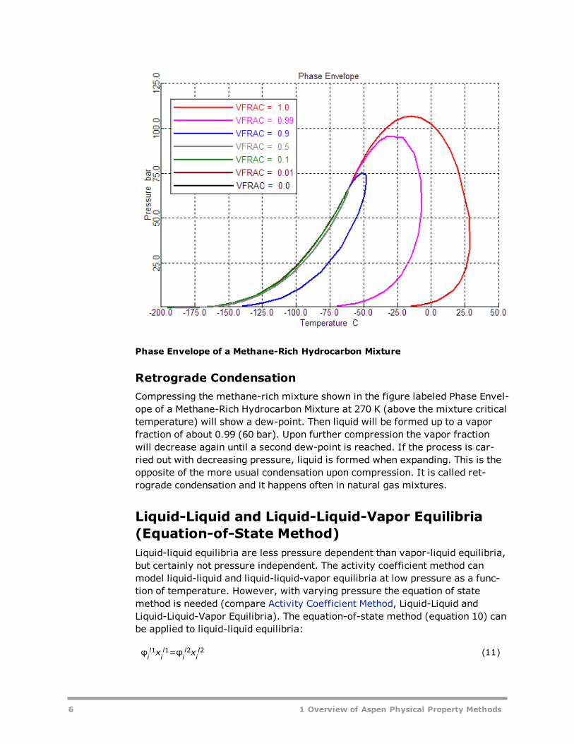
Phase Envelope of a Methane-Rich Hydrocarbon Mixture
Retrograde CondensationCompressing the methane-rich mixture shown in the figure labeled Phase Envel-ope of a Methane-Rich Hydrocarbon Mixture at 270 K (above the mixture criticaltemperature) will show a dew-point. Then liquid will be formed up to a vaporfraction of about 0.99 (60 bar). Upon further compression the vapor fractionwill decrease again until a second dew-point is reached. If the process is car-ried out with decreasing pressure, liquid is formed when expanding. This is theopposite of the more usual condensation upon compression. It is called ret-rograde condensation and it happens often in natural gas mixtures.
Liquid-Liquid and Liquid-Liquid-Vapor Equilibria(Equation-of-State Method)Liquid-liquid equilibria are less pressure dependent than vapor-liquid equilibria,but certainly not pressure independent. The activity coefficient method canmodel liquid-liquid and liquid-liquid-vapor equilibria at low pressure as a func-tion of temperature. However, with varying pressure the equation of statemethod is needed (compare Activity Coefficient Method, Liquid-Liquid andLiquid-Liquid-Vapor Equilibria). The equation-of-state method (equation 10) canbe applied to liquid-liquid equilibria:
φil1xi
l1=φil2xi
l2 (11)
6 1 Overview of Aspen Physical Property Methods

and also to liquid-liquid-vapor equilibria:
φivyi=φi
l1xil1=φi
l2xil2 (12)
Fugacity coefficients in all the phases are calculated using the same equation ofstate. Fugacity coefficients from equations of state are a function of com-position, temperature, and pressure. Therefore, the pressure dependency ofliquid-liquid equilibria can be described.
Liquid Phase NonidealityLiquid-liquid separation occurs in systems with very dissimilar molecules.Either the size or the intermolecular interactions between components may bedissimilar. Systems that demix at low pressures, have usually strongly dis-similar intermolecular interactions, as for example in mixtures of polar andnon-polar molecules. In this case, the miscibility gap is likely to exist at highpressures as well. An examples is the system dimethyl-ether and water ( Pozoand Street, 1984). This behavior also occurs in systems of a fully- or near fully-fluorinated aliphatic or alicyclic fluorocarbon with the corresponding hydro-carbon ( Rowlinson and Swinton, 1982), for example cyclohexane and per-fluorocyclohexane ( Dyke et al., 1959; Hicks and Young, 1971).
Systems which have similar interactions, but which are very different in size,do demix at higher pressures. For binary systems, this happens often in thevicinity of the critical point of the light component ( Rowlinson and Swinton,1982).
Examples are:
l Methane with hexane or heptane ( van der Kooi, 1981; Davenport andRowlinson, 1963; Kohn, 1961)
l Ethane with n-alkanes with carbon numbers from 18 to 26 ( Peters et al.,1986)
l Carbon dioxide with n-alkanes with carbon numbers from 7 to 20 ( Fall etal., 1985)
The more the demixing compounds differ in molecular size, the more likely it isthat the liquid-liquid and liquid-liquid-vapor equilibria will interfere with solid-ification of the heavy component. For example, ethane and pentacosane orhexacosane show this. Increasing the difference in carbon number furthercauses the liquid-liquid separation to disappear. For example in mixtures of eth-ane with n-alkanes with carbon numbers higher than 26, the liquid-liquid sep-aration becomes metastable with respect to the solid-fluid (gas or liquid)equilibria ( Peters et al., 1986). The solid cannot be handled by an equation-of-state method.
Critical Solution TemperatureIn liquid-liquid equilibria, mutual solubilities depend on temperature and pres-sure. Solubilities can increase or decrease with increasing or decreasing
1 Overview of Aspen Physical Property Methods 7

temperature or pressure. The trend depends on thermodynamic mixture prop-erties but cannot be predicted a priori. Immiscible phases can become misciblewith increasing or decreasing temperature or pressure. In that case a liquid-liquid critical point occurs. Equations 11 and 12 can handle this behavior, butengineering type equations of state cannot model these phenomena accurately.
Calculation of Properties Using an Equation-of-State Property MethodThe equation of state can be related to other properties through fundamentalthermodynamic equations :
l Fugacity coefficient:
f φ y p=iv
ivi
(13)
l Enthalpy departure:
∫H H pRT
VdV RT
V
V
T S S RT Z
( − ) = − − − ln
+ ( − ) + ( − 1)
m mig
V
ig
m mig
m
∞
(14)
l Entropy departure:
∫S Sp
T
R
VdV R
V
V( − ) = −
∂
∂− + lnm m
ig V
vig∞
(15)
l Gibbs energy departure:
∫G G pRT
VdV RT
V
VRT Z( − ) = − − − ln + ( − 1)m m
ig V
ig m∞
(16)
l Molar volume:Solve p(T,Vm) for Vm.
From a given equation of state, fugacities are calculated according to equation13. The other thermodynamic properties of a mixture can be computed fromthe departure functions:
l Vapor enthalpy:
H H H H= + ( − )mv
mig
mv
mig (17)
l Liquid enthalpy:
H H H H= + ( − )mv
mig
mv
mig (18)
The molar ideal gas enthalpy, Hmig is computed by the expression:
8 1 Overview of Aspen Physical Property Methods

∫∑H y H C T dT= ∆ + ( )mig
ii f i
ig
T
T
p iig,ref
(19)
Where:
Cp,iig = Ideal gas heat capacity
ΔfHiig = Standard enthalpy of formation for ideal gas at 298.15 K and 1 atm
Tref = Reference temperature = 298.15 K
Entropy and Gibbs energy can be computed in a similar manner:
G G G G= + ( − )mv
mig
mv
mig (20)
( )G G G G= + −ml
mig
ml
mig (21)
S S S S= + ( − )mv
mig
mv
mig (22)
( )S S S S= + −ml
mig
ml
mig (23)
Vapor and liquid volume is computed by solving p(T,Vm) for Vm or computed byan empirical correlation.
Advantages and Disadvantages of the Equation-of-State MethodYou can use equations of state over wide ranges of temperature and pressure,including subcritical and supercritical regions. For ideal or slightly non-ideal sys-tems, thermodynamic properties for both the vapor and liquid phases can becomputed with a minimum amount of component data. Equations of state aresuitable for modeling hydrocarbon systems with light gases such as CO2, N2,and H2S.
For the best representation of non-ideal systems, you must obtain binary inter-action parameters from regression of experimental vapor-liquid equilibrium(VLE) data. Equation of state binary parameters for many component pairs areavailable in the Aspen Physical Property System.
The assumptions in the simpler equations of state (Redlich-Kwong-Soave,Peng-Robinson, Lee-Kesler-Plöcker) are not capable of representing highly non-ideal chemical systems, such as alcohol-water systems. Use the activity-coef-ficient options sets for these systems at low pressures. At high pressures, usethe flexible and predictive equations of state.
Equations of state generally do a poor job at predicting liquid density. To com-pensate for this, PENG-ROB, LK-PLOCK, RK-SOAVE, and the methods based onthese calculate liquid density using the API correlation for pseudocomponents
1 Overview of Aspen Physical Property Methods 9
and the Rackett model for real components, rather than using the liquid densitypredicted by the equation of state. This is more accurate, but using causes aminor inconsistency which is mainly apparent for supercritical fluids, where thevapor and liquid properties should be the same, but the density will not be. Allother equation-of-state methods use the equation of state to calculate liquiddensity, except that SRK and some of the methods based on it correct this dens-ity with a volume translation term based on the Peneloux-Rauzy method.
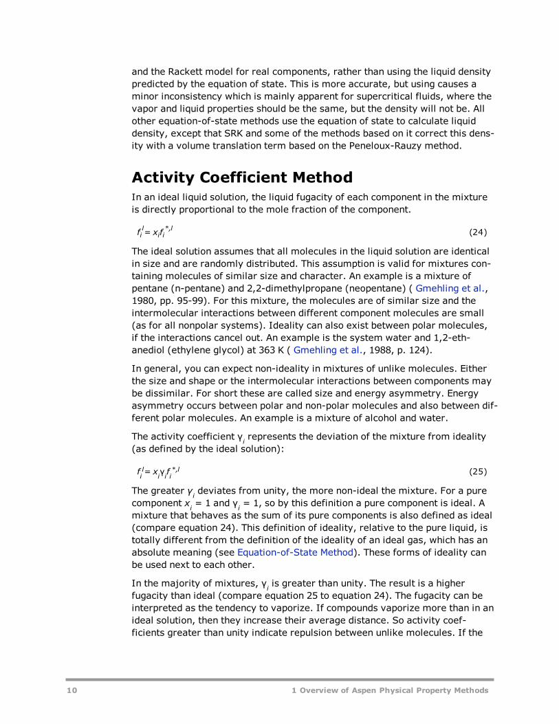
Activity Coefficient MethodIn an ideal liquid solution, the liquid fugacity of each component in the mixtureis directly proportional to the mole fraction of the component.
fil= xifi
*,l (24)
The ideal solution assumes that all molecules in the liquid solution are identicalin size and are randomly distributed. This assumption is valid for mixtures con-taining molecules of similar size and character. An example is a mixture ofpentane (n-pentane) and 2,2-dimethylpropane (neopentane) ( Gmehling et al.,1980, pp. 95-99). For this mixture, the molecules are of similar size and theintermolecular interactions between different component molecules are small(as for all nonpolar systems). Ideality can also exist between polar molecules,if the interactions cancel out. An example is the system water and 1,2-eth-anediol (ethylene glycol) at 363 K ( Gmehling et al., 1988, p. 124).
In general, you can expect non-ideality in mixtures of unlike molecules. Eitherthe size and shape or the intermolecular interactions between components maybe dissimilar. For short these are called size and energy asymmetry. Energyasymmetry occurs between polar and non-polar molecules and also between dif-ferent polar molecules. An example is a mixture of alcohol and water.
The activity coefficient γi represents the deviation of the mixture from ideality(as defined by the ideal solution):
fil= xiγifi
*,l (25)
The greater γi deviates from unity, the more non-ideal the mixture. For a purecomponent xi = 1 and γi = 1, so by this definition a pure component is ideal. Amixture that behaves as the sum of its pure components is also defined as ideal(compare equation 24). This definition of ideality, relative to the pure liquid, istotally different from the definition of the ideality of an ideal gas, which has anabsolute meaning (see Equation-of-State Method). These forms of ideality canbe used next to each other.
In the majority of mixtures, γi is greater than unity. The result is a higherfugacity than ideal (compare equation 25 to equation 24). The fugacity can beinterpreted as the tendency to vaporize. If compounds vaporize more than in anideal solution, then they increase their average distance. So activity coef-ficients greater than unity indicate repulsion between unlike molecules. If the
10 1 Overview of Aspen Physical Property Methods

repulsion is strong, liquid-liquid separation occurs. This is another mechanismthat decreases close contact between unlike molecules.
It is less common that γi is smaller than unity. Using the same reasoning, thiscan be interpreted as strong attraction between unlike molecules. In this case,liquid-liquid separation does not occur. Instead formation of complexes is pos-sible.
Vapor-Liquid Equilibria (Activity Coefficient Meth-ods)In the activity coefficient approach, the basic vapor-liquid equilibrium rela-tionship is represented by:
φivyip= xiγifi
*,l (26)
The vapor phase fugacity coefficient φiv is computed from an equation of state
(see Equation-of-State Method). The liquid activity coefficient γi is computedfrom an activity coefficient model.
For an ideal gas, φiv = 1. For an ideal liquid, γi = 1. Combining this with equa-
tion 26 gives Raoult's law:
yip= xipi*,l (27)
At low to moderate pressures, the main difference between equations 26 and27 is due to the activity coefficient. If the activity coefficient is larger thanunity, the system is said to show positive deviations from Raoults law. Negativedeviations from Raoult's law occur when the activity coefficient is smaller thanunity.
Liquid Phase Reference FugacityThe liquid phase reference fugacity fi
*,l from equation 26 can be computed inthree ways:
For solvents: The reference state for a solvent is defined as pure componentin the liquid state, at the temperature and pressure of the system. By this defin-ition γi approaches unity as xi approaches unity.
The liquid phase reference fugacity fi*,l is computed as:
fi*,l=φi
*,v(T, pi*,l) pi
*,lθi*,l (28)
Where:
φi*,v = Fugacity coefficient of pure component i at the system temperature and
vapor pressures, as calculated from the vapor phase equation of state
pi*,l = Liquid vapor pressures of component i at the system temperature
θi*,l = Poynting correction for pressure
1 Overview of Aspen Physical Property Methods 11

=
∫RTV dpexp
1*
p
p
il
*,
il,
At low pressures, the Poynting correction is near unity, and can be ignored.
For dissolved gases: Light gases (such as O2 and N2) are usually supercriticalat the temperature and pressure of the solution. In that case pure componentvapor pressure is meaningless and therefore it cannot serve as the referencefugacity. The reference state for a dissolved gas is redefined to be at infinitedilution and at the temperature and pressure of the mixtures. The liquid phasereference fugacity fi
*,l becomes Hi (the Henry's constant for component i in themixture).
The activity coefficient γi is converted to the infinite dilution reference statethrough the relationship:
( )γ γ γ* = /i i
∞ (29)
Where:
γi∞ = The infinite dilution activity coefficient of component i in the mixture
By this definition γ* approaches unity as xi approaches zero. The phase equi-librium relationship for dissolved gases becomes:
φivyip= xiγi*Hi (30)
To compute Hi, you must supply the Henry's constant for the dissolved-gas com-ponent i in each subcritical solvent component.
Using an Empirical Correlation: The reference state fugacity is calculatedusing an empirical correlation. Examples are the Chao-Seader or the Grayson-Streed model.
Electrolyte and Multicomponent VLEThe vapor-liquid equilibrium equations 26 and 30, only apply for componentswhich occur in both phases. Ions are components which do not participate dir-ectly in vapor-liquid equilibrium. This is true as well for solids which do not dis-solve or vaporize. However, ions influence activity coefficients of the otherspecies by interactions. As a result they participate indirectly in the vapor-liquid equilibria. An example is the lowering of the vapor pressure of a solutionupon addition of an electrolyte. For more on electrolyte activity coefficient mod-els, see Activity Coefficient Models.
Multicomponent vapor-liquid equilibria are calculated from binary parameters.These parameters are usually fitted to binary phase equilibrium data (and notmulticomponent data) and represent therefore binary information. The pre-
12 1 Overview of Aspen Physical Property Methods

diction of multicomponent phase behavior from binary information is generallygood.
Liquid-Liquid and Liquid-Liquid-Vapor Equilibria(Activity Coefficient Method)The basic liquid-liquid-vapor equilibrium relationship is:
x γ f x γ f φ y p* = * =ililil
ililil
ivi
1 1 , 2 2 , (31)
Equation 31 can be derived from the liquid-vapor equilibrium relationship byanalogy. For liquid-liquid equilibria, the vapor phase term can be omitted, andthe pure component liquid fugacity cancels out:
x γ x γ=ilil
ilil1 1 2 2 (32)
The activity coefficients depend on temperature, and so do liquid-liquid equi-libria. However, equation 32 is independent of pressure. The activity coefficientmethod is very well suited for liquid-liquid equilibria at low to moderate pres-sures. Mutual solubilities do not change with pressure in this case. For high-pressure liquid-liquid equilibria, mutual solubilities become a function of pres-sure. In that case, use an equation-of-state method.
For the computation of the different terms in equations 31 and 32, see Vapor-Liquid Equilibria.
Multi-component liquid-liquid equilibria cannot be reliably predicted from bin-ary interaction parameters fitted to binary data only. In general, regression ofbinary parameters from multi-component data will be necessary. See Regress-ing Property Data in the help for details.
The ability of activity coefficient models in describing experimental liquid-liquidequilibria differs. The Wilson model cannot describe liquid-liquid separation atall; UNIQUAC, UNIFAC and NRTL are suitable. For details, see Activity Coef-ficient Models. Activity coefficient models sometimes show anomalous behaviorin the metastable and unstable composition region. Phase equilibrium cal-culation using the equality of fugacities of all components in all phases (as inequations 31 and 32), can lead to unstable solutions. Instead, phase equilibriumcalculation using the minimization of Gibbs energy always yields stable solu-tions.
The figure labeled (T,x,x,y)—Diagram of Water and Butanol-1 at 1.01325 bar, agraphical Gibbs energy minimization of the system n-butanol + water, showsthis.
1 Overview of Aspen Physical Property Methods 13

(T,x,x,y)—Diagram of Water and Butanol-1 at 1.01325 bar
The phase diagram of n-butanol + water at 1 bar is shown in this figure. Thereis liquid-liquid separation below 367 K and there are vapor-liquid equilibriaabove this temperature. The diagram is calculated using the UNIFAC activitycoefficient model with the liquid-liquid data set.
The Gibbs energies† of vapor and liquid phases at 1 bar and 365 K are given inthe figure labeled Molar Gibbs Energy of Butanol-1 and Water at 365 K and 1atm. This corresponds to a section of the phase diagram at 365 K. The Gibbsenergy of the vapor phase is higher than that of the liquid phase at any molefraction. This means that the vapor is unstable with respect to the liquid atthese conditions. The minimum Gibbs energy of the system as a function of themole fraction can be found graphically by stretching an imaginary string frombelow around the Gibbs curves. For the case of the figure labeled Molar GibbsEnergy of Butanol-1 and Water at 365 K and 1 atm, the string never touches thevapor Gibbs energy curve. For the liquid the situation is more subtle: the stringtouches the curve at the extremities but not at mole fractions between 0.56 and0.97. In that range the string forms a double tangent to the curve. A hypo-thetical liquid mixture with mole fraction of 0.8 has a higher Gibbs energy andis unstable with respect to two liquid phases with mole fractions correspondingto the points where the tangent and the curve touch. The overall Gibbs energyof these two phases is a linear combination of their individual Gibbs energiesand is found on the tangent (on the string). The mole fractions of the two liquidphases found by graphical Gibbs energy minimization are also indicated in thefigure labeled (T,x,x,y)—Diagram of Water and Butanol-1 at 1.01325 bar.
14 1 Overview of Aspen Physical Property Methods

Molar Gibbs Energy of Butanol-1 and Water at 365 K and 1 atm
† The Gibbs energy has been transformed by a contribution linear in themole fraction, such that the Gibbs energy of pure liquid water (ther-modynamic potential of water) has been shifted to the value of pure liquidn-butanol. This is done to make the Gibbs energy minimization visible onthe scale of the graph. This transformation has no influence on the resultof Gibbs energy minimization (Oonk, 1981).
At a temperature of 370 K, the vapor has become stable in the mole fractionrange of 0.67 to 0.90 (see the figure labeled Molar Gibbs Energy of Butanol-1and Water at 370 K and 1 atm). Graphical Gibbs energy minimization results intwo vapor-liquid equilibria, indicated in the figure labeled Molar Gibbs Energy ofButanol-1 and Water at 370 K and 1 atm. Ignoring the Gibbs energy of thevapor and using a double tangent to the liquid Gibbs energy curve a liquid-liquidequilibrium is found. This is unstable with respect to the vapor-liquid equilibria.This unstable equilibrium will not be found with Gibbs minimization (unless thevapor is ignored) but can easily be found with the method of equality of fugacit-ies.
1 Overview of Aspen Physical Property Methods 15

Molar Gibbs Energy of Butanol-1 and Water at 370 K and 1 atm
The technique of Gibbs energy minimization can be used for any number ofphases and components, and gives accurate results when handled by a com-puter algorithm. This technique is always used in the equilibrium reactor unitoperation model RGibbs, and can be used optionally for liquid phase separationin the distillation model RadFrac.
Phase Equilibria Involving SolidsIn most instances, solids are treated as inert with respect to phase equilibrium(CISOLID). This is useful if the components do not dissolve or vaporize. Anexample is sand in a water stream. CISOLID components may be stored in sep-arate substreams or in the MIXED substream.
There are two areas of application where phase equilibrium involving solidsmay occur:
l Salt precipitation in electrolyte solutionsl Pyrometallurgical applications
Salt PrecipitationElectrolytes in solution often have a solid solubility limit. Solid solubilities canbe calculated if the activity coefficients of the species and the solubility productare known (for details see Electrolyte Calculation). The activity of the ionic spe-cies can be computed from an electrolyte activity coefficient model (see Activ-ity Coefficient Models). The solubility product can be computed from the Gibbsenergies of formation of the species participating in the precipitation reaction
16 1 Overview of Aspen Physical Property Methods

or can be entered as the temperature function (K-SALT) on the Chemistry |Equilibrium Constants sheet.
Salt precipitation is only calculated when the component is declared as a Salton the Chemistry | Stoichiometry sheet. The salt components are part of theMIXED substream, because they participate in phase equilibrium. The types ofequilibria are liquid-solid or vapor-liquid-solid. Each precipitating salt is treatedas a separate, pure component, solid phase.
Solid compounds, which are composed of stoichiometric amounts of other com-ponents, are treated as pure components. Examples are salts with crystalwater, like CaSO4, H2O.
Phase Equilibria Involving Solids for Metallurgical Applic-ationsMineral and metallic solids can undergo phase equilibria in a similar way asorganic liquids. Typical pyrometallurgical applications have specific char-acteristics:
l Simultaneous occurrence of multiple solid and liquid phasesl Occurrence of simultaneous phase and chemical equilibrial Occurrence of mixed crystals or solid solutions
These specific characteristics are incompatible with the chemical and phaseequilibrium calculations by flash algorithms as used for chemical and pet-rochemical applications. Instead, these equilibria can be calculated by usingGibbs energy minimization techniques. In Aspen Plus, the unit operation modelRGibbs is specially designed for this purpose.
Gibbs energy minimization techniques are equivalent to phase equilibrium com-putations based on equality of fugacities. If the distribution of the componentsof a system is found, such that the Gibbs energy is minimal, equilibrium isobtained. (Compare the discussion of phase equilibrium calculation using Gibbsenergy minimization in Liquid-Liquid and Liquid-Liquid-Vapor Equilibria)
As a result, the analog of equation 31 holds:
x γ f x γ f x γ f x γ f φ y p* = * = ... * = * = ...ililil
ililil
isisis
isisis
ivi
1 1 , 2 2 , 1 1 , 2 2 , (33)
This equation can be simplified for pure component solids and liquids, or beextended for any number of phases.
For example, the pure component vapor pressure (or sublimation) curve can becalculated from the pure component Gibbs energies of vapor and liquid (orsolid). The figure labeled Thermodynamic Potential of Mercury at 1, 5, 10, and20 bar shows the pure component molar Gibbs energy or thermodynamic poten-tial of liquid and vapor mercury as a function of temperature and at four dif-ferent pressures: 1,5,10 and 20 bar†. The thermodynamic potential of the liquidis not dependent on temperature and independent of pressure: the four curves
1 Overview of Aspen Physical Property Methods 17

coincide. The vapor thermodynamic potential is clearly different at each pres-sure. The intersection point of the liquid and vapor thermodynamic potentials at1 bar is at about 630 K. At this point the thermodynamic potentials of the twophases are equal, so there is equilibrium. A point of the vapor pressure curve isfound. Below this temperature the liquid has the lower thermodynamic poten-tial and is the stable phase; above this temperature the vapor has the lowerthermodynamic potential. Repeating the procedure for all four pressures givesthe four points indicated on the vapor pressure curve (see the figure labeledVapor Pressure Curve of Liquid Mercury). This is a similar result as a direct cal-culation with the Antoine equation. The procedure can be repeated for a largenumber of pressures to construct the curve with sufficient accuracy. The sub-limation curve can also be calculated using an Antoine type model, similar tothe vapor pressure curve of a liquid.
Thermodynamic Potential of Mercury at 1, 5, 10, and 20 bar
†The pure component molar Gibbs energy is equal to the pure componentthermodynamic potential. The ISO and IUPAC recommendation to use thethermodynamic potential is followed.
18 1 Overview of Aspen Physical Property Methods

Vapor Pressure Curve of Liquid Mercury
The majority of solid databank components occur in the INORGANIC databank.In that case, pure component Gibbs energy, enthalpy and entropy of solid,liquid or vapor are calculated by polynomials (see Physical Property Models).
The pure component solid properties (Gibbs energy and enthalpy) together withthe liquid and vapor mixture properties are sufficient input to calculate chem-ical and phase equilibria involving pure solid phases. In some cases mixed crys-tals or solid solutions can occur. These are separate phases. The concept ofideality and nonideality of solid solutions are similar to those of liquid phases(see Vapor-Liquid Equilibria). The activity coefficient models used to describenonideality of the solid phase are different than those generally used for liquidphases. However some of the models (Margules, Redlich-Kister) can be usedfor liquids as well. If multiple liquid and solid mixture phases occur sim-ultaneously, the activity coefficient models used can differ from phase tophase.
To be able to distinguish pure component solids from solid solutions in thestream summary, the pure component solids are placed in the CISOLID sub-stream and the solid solutions in the MIXED substream, when the CISOLID sub-stream exists.
1 Overview of Aspen Physical Property Methods 19

Calculation of Other Properties Using Activity Coef-ficientsProperties can be calculated for vapor, liquid or solid phases:
Vapor phase: Vapor enthalpy, entropy, Gibbs energy and density are com-puted from an equation of state (see Calculation of Properties Using an Equa-tion-of-State Property Method).
Liquid phase: Liquid mixture enthalpy is computed as:
( )∑H x H H H= * − ∆ * +ml
i
i iv
vap i mE l, , (34)
Where:
Hi*,v = Pure component vapor enthalpy at T and vapor pressure
ΔvapHi* = Component vaporization enthalpy
HmE,l = Excess liquid enthalpy
Excess liquid enthalpy HmE,l is related to the activity coefficient through the
expression:
∑H RT xγ
T= −
∂ln
∂mE l
i
ii, 2
(35)
Liquid mixture Gibbs free energy and entropy are computed as:
( )STH G=
1−m
lml
ml (36)
∑G G RT φ G= − ln * +ml
mv
iil
mE l, , (37)
Where:
∑G RT x γ= lnmE l
i
i i, (38)
Liquid density is computed using an empirical correlation.
Solid phase: Solid mixture enthalpy is computed as:
∑H x H H= * +m
s
i
i
s
i
s
m
E s, , (39)
Where:
20 1 Overview of Aspen Physical Property Methods

Hi*,s = Pure component solid enthalpy at T
HmE,s = The excess solid enthalpy
Excess solid enthalpy HmE,s is related to the activity coefficient through the
expression:
∑H RT xγ
T= −
∂ln
∂mE s
i
ii, 2
(40)
Solid mixture Gibbs energy is computed as:
∑ ∑G x G RT x x= µ* + + lnms
i
i i
smE s
i
is
is, , (41)
Where:
∑G RT x γ= lnmE s
i
is
is, (42)
The solid mixture entropy follows from the Gibbs energy and enthalpy:
STH G=
1( − )m
sms
ms (43)
Advantages and Disadvantages of the Activity Coef-ficient MethodThe activity coefficient method is the best way to represent highly non-idealliquid mixtures at low pressures. You must estimate or obtain binary para-meters from experimental data, such as phase equilibrium data. Binary para-meters for the Wilson, NRTL, and UNIQUAC models are available in the AspenPhysical Property System for a large number of component pairs. These binaryparameters are used automatically. See Binary Parameters for Activity Coef-ficient Models in Physical Property Data in the help, for details.
Binary parameters are valid only over the temperature and pressure ranges ofthe data. Binary parameters outside the valid range should be used with cau-tion, especially in liquid-liquid equilibrium applications. If no parameters areavailable, the predictive UNIFAC models can be used.
The activity coefficient approach should be used only at low pressures (below10 atm). For systems containing dissolved gases at low pressures and at smallconcentrations, use Henry's law. For highly non-ideal chemical systems at highpressures, use the flexible and predictive equations of state.
1 Overview of Aspen Physical Property Methods 21
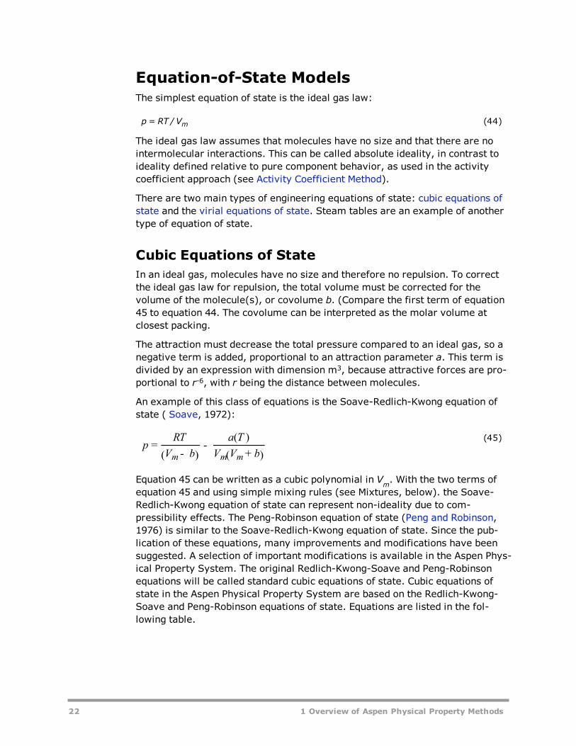
Equation-of-State ModelsThe simplest equation of state is the ideal gas law:
p= RT / Vm (44)
The ideal gas law assumes that molecules have no size and that there are nointermolecular interactions. This can be called absolute ideality, in contrast toideality defined relative to pure component behavior, as used in the activitycoefficient approach (see Activity Coefficient Method).
There are two main types of engineering equations of state: cubic equations ofstate and the virial equations of state. Steam tables are an example of anothertype of equation of state.
Cubic Equations of StateIn an ideal gas, molecules have no size and therefore no repulsion. To correctthe ideal gas law for repulsion, the total volume must be corrected for thevolume of the molecule(s), or covolume b. (Compare the first term of equation45 to equation 44. The covolume can be interpreted as the molar volume atclosest packing.
The attraction must decrease the total pressure compared to an ideal gas, so anegative term is added, proportional to an attraction parameter a. This term isdivided by an expression with dimension m3, because attractive forces are pro-portional to r-6, with r being the distance between molecules.
An example of this class of equations is the Soave-Redlich-Kwong equation ofstate ( Soave, 1972):
pRT
V b
a T
V V b=( − )
−( )
( + )m m m
(45)
Equation 45 can be written as a cubic polynomial in Vm. With the two terms ofequation 45 and using simple mixing rules (see Mixtures, below). the Soave-Redlich-Kwong equation of state can represent non-ideality due to com-pressibility effects. The Peng-Robinson equation of state (Peng and Robinson,1976) is similar to the Soave-Redlich-Kwong equation of state. Since the pub-lication of these equations, many improvements and modifications have beensuggested. A selection of important modifications is available in the Aspen Phys-ical Property System. The original Redlich-Kwong-Soave and Peng-Robinsonequations will be called standard cubic equations of state. Cubic equations ofstate in the Aspen Physical Property System are based on the Redlich-Kwong-Soave and Peng-Robinson equations of state. Equations are listed in the fol-lowing table.
22 1 Overview of Aspen Physical Property Methods

Cubic Equations of State in the Aspen Physical Property Sys-tem
Redlich-Kwong(-Soave) based Peng-Robinson based
Redlich-Kwong Standard Peng-Robinson
Standard Redlich-Kwong-Soave Peng-Robinson
Redlich-Kwong-Soave Peng-Robinson-MHV2
Redlich-Kwong-ASPEN Peng-Robinson-WS
Schwartzentruber-Renon
Redlich-Kwong-Soave-MHV2
Predictive SRK
Redlich-Kwong-Soave-WS
Pure ComponentsIn a standard cubic equation of state, the pure component parameters are cal-culated from correlations based on critical temperature, critical pressure, andacentric factor. These correlations are not accurate for polar compounds orlong chain hydrocarbons. Introducing a more flexible temperature dependencyof the attraction parameter (the alpha-function), the quality of vapor pressurerepresentation improves. Up to three different alpha functions are built-in tothe following cubic equation-of-state models in the Aspen Physical Property Sys-tem: Redlich-Kwong-Aspen, Schwartzenruber-Renon, Peng-Robinson-MHV2,Peng-Robinson-WS, Predictive RKS, Redlich-Kwong-Soave-MHV2, and Redlich-Kwong-Soave-WS.
Cubic equations of state do not represent liquid molar volume accurately. Tocorrect this you can use volume translation, which is independent of VLE com-putation. The Schwartzenruber-Renon equation of state model has volumetranslation.
MixturesThe cubic equation of state calculates the properties of a fluid as if it consistedof one (imaginary) component. If the fluid is a mixture, the parameters a and bof the imaginary component must be calculated from the pure component para-meters of the real components, using mixing rules. The classical mixing rules,with one binary interaction parameter for the attraction parameter, are not suf-ficiently flexible to describe mixtures with strong shape and size asymmetry:
( )∑∑a x x a a k= ( ) 1 −
i j
i j i j a ij,1/2 (46)
1 Overview of Aspen Physical Property Methods 23

∑ ∑∑b x b x xb b
= =+
2i
i i
i j
i ji j
(47)
A second interaction coefficient is added for the b parameter in the Redlich-Kwong-Aspen ( Mathias, 1983) and Schwartzentruber-Renon ( Schwartzen-truber and Renon, 1989) equations of state:
( )∑∑b x xb b
k=+
21 −
i j
i ji j
b ij,
(48)
This is effective to fit vapor-liquid equilibrium data for systems with strong sizeand shape asymmetry but it has the disadvantage that kb,ij is strongly cor-related with ka,ij and that kb,ij affects the excess molar volume ( Lermite andVidal, 1988).
For strong energy asymmetry, in mixtures of polar and non-polar compounds,the interaction parameters should depend on composition to achieve thedesired accuracy of representing VLE data. Huron-Vidal mixing rules use activ-ity coefficient models as mole fraction functions ( Huron and Vidal, 1979).These mixing rules are extremely successful in fitting because they combinethe advantages of flexibility with a minimum of drawbacks ( Lermite and Vidal,1988). However, with the original Huron-Vidal approach it is not possible to useactivity coefficient parameters, determined at low pressures, to predict thehigh pressure equation-of-state interactions.
Several modifications of Huron-Vidal mixing rules exist which use activity coef-ficient parameters obtained at low pressure directly in the mixing rules (see thetable labeled Cubic Equations of State in the Aspen Physical Property System).They accurately predict binary interactions at high pressure. In practice thismeans that the large database of activity coefficient data at low pressures(DECHEMA Chemistry Data Series, Dortmund DataBank) is now extended tohigh pressures.
The MHV2 mixing rules ( Dahl and Michelsen, 1990), use the Lyngby modifiedUNIFAC activity coefficient model (See Activity Coefficient Models). The qualityof the VLE predictions is good.
The Predictive SRKmethod ( Holderbaum and Gmehling, 1991; Fischer, 1993)uses the original UNIFAC model. The prediction of VLE is good. The mixing rulescan be used with any equation of state, but it has been integrated with the Red-lich-Kwong-Soave equation of state in the following way: new UNIFAC groupshave been defined for gaseous components, such as hydrogen. Interaction para-meters for the new groups have been regressed and added to the existing para-meter matrix. This extends the existing low pressure activity coefficient data tohigh pressures, and adds prediction of gas solubilities at high pressures.
24 1 Overview of Aspen Physical Property Methods
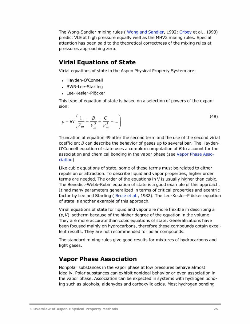
The Wong-Sandler mixing rules ( Wong and Sandler, 1992; Orbey et al., 1993)predict VLE at high pressure equally well as the MHV2 mixing rules. Specialattention has been paid to the theoretical correctness of the mixing rules atpressures approaching zero.
Virial Equations of StateVirial equations of state in the Aspen Physical Property System are:
l Hayden-O'Connelll BWR-Lee-Starlingl Lee-Kesler-Plöcker
This type of equation of state is based on a selection of powers of the expan-sion:
p RTV
B
V
C
V=
1+ + + ...
m m m2 3
(49)
Truncation of equation 49 after the second term and the use of the second virialcoefficient B can describe the behavior of gases up to several bar. The Hayden-O'Connell equation of state uses a complex computation of B to account for theassociation and chemical bonding in the vapor phase (see Vapor Phase Asso-ciation).
Like cubic equations of state, some of these terms must be related to eitherrepulsion or attraction. To describe liquid and vapor properties, higher orderterms are needed. The order of the equations in V is usually higher than cubic.The Benedict-Webb-Rubin equation of state is a good example of this approach.It had many parameters generalized in terms of critical properties and acentricfactor by Lee and Starling ( Brulé et al., 1982). The Lee-Kesler-Plöcker equationof state is another example of this approach.
Virial equations of state for liquid and vapor are more flexible in describing a(p,V) isotherm because of the higher degree of the equation in the volume.They are more accurate than cubic equations of state. Generalizations havebeen focused mainly on hydrocarbons, therefore these compounds obtain excel-lent results. They are not recommended for polar compounds.
The standard mixing rules give good results for mixtures of hydrocarbons andlight gases.
Vapor Phase AssociationNonpolar substances in the vapor phase at low pressures behave almostideally. Polar substances can exhibit nonideal behavior or even association inthe vapor phase. Association can be expected in systems with hydrogen bond-ing such as alcohols, aldehydes and carboxylic acids. Most hydrogen bonding
1 Overview of Aspen Physical Property Methods 25

leads to dimers. HF is an exception; it forms mainly hexamers. This sectionuses dimerization as an example to discuss the chemical theory used todescribe strong association. Chemical theory can be used for any type of reac-tion.
If association occurs, chemical reactions take place. Therefore, a model basedon physical forces is not sufficient. Some reasons are:
l Two monomer molecules form one dimer molecule, so the total numberof species decreases. As a result the mole fractions change. This hasinfluence on VLE and molar volume (density).
l The heat of reaction affects thermal properties like enthalpy, Cp.
The equilibrium constant of a dimerization reaction,
A A2 ↔ 2 (50)
in the vapor phase is defined in terms of fugacities:
Kf
f=
A
A2
2
(51)
With:
fiv = φi
vyip (52)
and realizing that φiv is approximately unity at low pressures:
Ky
y p=
A
A2
2(53)
Equations 51-53 are expressed in terms of true species properties. This mayseem natural, but unless measurements are done, the true compositions arenot known. On the contrary, the composition is usually given in terms of unre-acted or apparent species (Abbott and van Ness, 1992), which represents theimaginary state of the system if no reaction takes place. Superscripts t and aare used to distinguish clearly between true and apparent species. (For moreon the use of apparent and true species approach, see Apparent Component andTrue Component Approaches in Physical Property Methods).
K in equation 53 is only a function of temperature. If the pressure approaches
zero at constant temperature,
y
y
A
A2
2
,which is a measure of the degree of asso-ciation, must decrease. It must go to zero for zero pressure where the ideal gasbehavior is recovered. The degree of association can be considerable at atmo-spheric pressure: for example acetic acid at 293 K and 1 bar is dimerized atabout 95% ( Prausnitz et al., 1986).
26 1 Overview of Aspen Physical Property Methods

The equilibrium constant is related to the thermodynamic properties of reac-tion:
KG
RT
H
RT
S
Rln = −
∆= −∆
+∆r r r (54)
The Gibbs energy, the enthalpy, and the entropy of reaction can be approx-imated as independent of temperature. Then from equation 54 it follows that lnK plotted against 1/T is approximately a straight line with a positive slope(since the reaction is exothermic) with increasing 1/T. This represents adecrease of ln K with increasing temperature. From this it follows (using equa-tion 53) that the degree of association decreases with increasing temperature.
It is convenient to calculate equilibria and to report mole fractions in terms ofapparent components. The concentrations of the true species have to be cal-culated, but are not reported. Vapor-liquid equilibria in terms of apparent com-ponents require apparent fugacity coefficients.
The fugacity coefficients of the true species are expected to be close to unity(ideal) at atmospheric pressure. However the apparent fugacity coefficientneeds to reflect the decrease in apparent partial pressure caused by thedecrease in number of species.
The apparent partial pressure is represented by the term yiap in the vapor
fugacity equation applied to apparent components:
fia,v = φi
a,vyiap (55)
In fact the apparent and true fugacity coefficients are directly related to eachother by the change in number of components ( Nothnagel et al., 1973; Abbottand van Ness, 1992):
φ φy
y=
ia v
it v i
t
ia
, ,(56)
1 Overview of Aspen Physical Property Methods 27

Apparent Fugacity of Vapor Benzene and Propionic Acid
This is why apparent fugacity coefficients of associating species are well belowunity. This is illustrated in the figure labeled Apparent Fugacity of Vapor Ben-zene and Propionic Acid for the system benzene + propionic acid at 415 K and101.325 kPa (1 atm) ( Nothnagel et al., 1973). The effect of dimerizationclearly decreases below apparent propionic acid mole fractions of about 0.2(partial pressures of 20 kPa). The effect vanishes at partial pressures of zero,as expected from the pressure dependence of equation 53. The apparentfugacity coefficient of benzene increases with increasing propionic acid molefraction. This is because the true mole fraction of propionic acid is higher thanits apparent mole fraction (see equation 56).
The vapor enthalpy departure needs to be corrected for the heat of association.The true heat of association can be obtained from the equilibrium constant:
H Td G
dTRT
d K
dT∆ = −
(∆ )=
(ln )r mt r m
t2 2
(57)
The value obtained from equation 57 must be corrected for the ratio of true toapparent number of species to be consistent with the apparent vapor enthalpydeparture. With the enthalpy and Gibbs energy of association (equations 57 and54), the entropy of association can be calculated.
The apparent heat of vaporization of associating components as a function oftemperature can show a maximum. The increase of the heat of vaporizationwith temperature is probably related to the decrease of the degree of
28 1 Overview of Aspen Physical Property Methods

association with increasing temperature. However, the heat of vaporizationmust decrease to zero when the temperature approaches the critical tem-perature. The figure labeled Liquid and Vapor Enthalpy of Acetic Acid illustratesthe enthalpic behavior of acetic acid. Note that the enthalpy effect due to asso-ciation is very large.
Liquid and Vapor Enthalpy of Acetic Acid
The true molar volume of an associating component is close to the true molarvolume of a non-associating component. At low pressures, where the ideal gaslaw is valid, the true molar volume is constant and equal to p/RT, independentof association. This means that associated molecules have a higher molecularmass than their monomers, but they behave as an ideal gas, just as theirmonomers. This also implies that the mass density of an associated gas ishigher than that of a gas consisting of the monomers. The apparent molarvolume is defined as the true total volume per apparent number of species.Since the number of apparent species is higher than the true number of speciesthe apparent molar volume is clearly smaller than the true molar volume.
The chemical theory can be used with any equation of state to compute truefugacity coefficients. At low pressures, the ideal gas law can be used.
For dimerization, two approaches are commonly used: the Nothagel and theHayden-O'Connel equations of state. For HF hexamerization a dedicated equa-tion of state is available in the Aspen Physical Property System.
Nothnagel et al. (1973) used a truncated van der Waals equation of state. Theycorrelated the equilibrium constants with the covolume b, a polarity parameterp and the parameter d. b can be determined from group contribution methods(Bondi, 1968) (or a correlation of the critical temperature and pressure (as in
1 Overview of Aspen Physical Property Methods 29

the Aspen Physical Property System). d and p are adjustable parameters. Manyvalues for d and p are available in the Nothnagel equation of state in the AspenPhysical Property System. Also correction terms for the heats of association ofunlike molecules are built-in. The equilibrium constant, K, has been correlatedto Tb, Tc, b, d, and p.
Hayden and O'Connell (1975) used the virial equation of state (equation 49),truncated after the second term. They developed a correlation for the secondvirial coefficient of polar, nonpolar and associating species based on the criticaltemperature and pressure, the dipole moment and the mean radius of gyration.Association of like and unlike molecules is described with the adjustable para-meter η. Pure component and binary values for η are available in the AspenPhysical Property System.
The HF equation of state ( de Leeuw and Watanasiri, 1993) assumes the form-ation of hexamers only. The fugacities of the true species are assumed to beideal, and is therefore suited for low pressures. Special attention has been paidto the robustness of the algorithm, and the consistency of the results with the-ory. The equation of state has been integrated with the electrolyte NRTL activitycoefficient model to allow the rigorous representation of absorption and strip-ping of HF with water. It can be used with other activity coefficient models forhydrocarbon + HF mixtures.
Activity Coefficient ModelsThis section discusses the characteristics of activity coefficient models. Thedescription is divided into the following categories:
l Molecular models (correlative models for non-electrolyte solutions)l Group contribution models (predictive models for non-electrolyte solu-tions)
l Electrolyte activity coefficient models
Molecular ModelsThe early activity coefficient models such as van Laar and Scatchard-Hildebrand, are based on the same assumptions and principles of regular solu-tions. Excess entropy and excess molar volume are assumed to be zero, andfor unlike interactions, London's geometric mean rule is used. Binary para-meters were estimated from pure component properties. The van Laar model isonly useful as correlative model. The Scatchard-Hildebrand can predict inter-actions from solubility parameters for non-polar mixtures. Both models predictonly positive deviations from Raoult's law (see Activity Coefficient Method).
The three-suffix Margules and the Redlich-Kister activity coefficient models areflexible arithmetic expressions.
Local composition models are very flexible, and the parameters have muchmore physical significance. These models assume ordering of the liquid
30 1 Overview of Aspen Physical Property Methods

solution, according to the interaction energies between different molecules. TheWilson model is suited for many types of non-ideality but cannot model liquid-liquid separation. The NRTL and UNIQUAC models can be used to describe VLE,LLE and enthalpic behavior of highly non-ideal systems. The WILSON, NRTL andUNIQUAC models are well accepted and are used on a regular basis to modelhighly non-ideal systems at low pressures.
A detailed discussion of molecular activity coefficient models and underlyingtheories can be found in Prausnitz et al. (1986).
Group Contribution ModelsThe UNIFAC activity coefficient model is an extension of the UNIQUAC model.It applies the same theory to functional groups that UNIQUAC uses formolecules. A limited number of functional groups is sufficient to form an infinitenumber of different molecules. The number of possible interactions betweengroups is very small compared to the number of possible interactions betweencomponents from a pure component database (500 to 2000 components).Group-group interactions determined from a limited, well chosen set of exper-imental data are sufficient to predict activity coefficients between almost anypair of components.
UNIFAC (Fredenslund et al., 1975; 1977) can be used to predict activity coef-ficients for VLE. For LLE a different dataset must be used. Mixture enthalpies,derived from the activity coefficients (see Activity Coefficient Method) are notaccurate.
UNIFAC has been modified at the Technical University of Lyngby (Denmark).The modification includes an improved combinatorial term for entropy and thegroup-group interaction has been made temperature dependent. The threeUNIFAC models are available in the Aspen Physical Property System. Fordetailed information on each model, see Physical Property Models.
This model can be applied to VLE, LLE and enthalpies ( Larsen et al., 1987).Another UNIFAC modification comes from the University of Dortmund (Ger-many). This modification is similar to Lyngby modified UNIFAC, but it can alsopredict activity coefficients at infinite dilution ( Weidlich and Gmehling, 1987).
Electrolyte ModelsIn electrolyte solutions a larger variety of interactions and phenomena existthan in non-electrolyte solutions. Besides physical and chemical molecule-molecule interactions, ionic reactions and interactions occur (molecule-ion andion-ion). Electrolyte activity coefficient models (Electrolyte NRTL, Pitzer) aretherefore more complicated than non-electrolyte activity coefficient models.Electrolytes dissociate so a few components can form many species in a solu-tion. This causes a multitude of interactions, some of which are strong. This sec-tion gives a summary of the capabilities of the electrolyte activity coefficient
1 Overview of Aspen Physical Property Methods 31

models in the Aspen Physical Property System. For details, see Physical Prop-erty Models.
The Pitzer electrolyte activity coefficient model can be used for the rep-resentation of aqueous electrolyte solutions up to 6 molal strength (literaturereferences: Chen et al., 1979; Fürst and Renon, 1982; Guggenheim, 1935; Gug-genheim and Turgeon, 1955; Renon, 1981). The model handles gas solubilities.Excellent results can be obtained, but many parameters are needed.
The Electrolyte NRTL model is an extension of the molecular NRTL model (lit-erature references: Chen et al., 1982; Chen and Evans, 1986; CRC Handbook,1975; Mock et al., 1984, 1986; Renon and Prausnitz, 1968). It can handle elec-trolyte solutions of any strength, and is suited for solutions with multiplesolvents, and dissolved gases. The flexibility of this model makes it very suit-able for any low-to-moderate pressure application.
Electrolyte parameter databanks and data packages for industrially importantapplications have been developed for both models (see Physical PropertyData). If parameters are not available, use data regression, or the Bromley-Pitzer activity coefficient model.
The Bromley-Pitzer activity coefficient model is a simplification of the Pitzermodel (literature references: Bromley, 1973; Fürst and Renon, 1982). A cor-relation is used to calculate the interaction parameters. The model is limited inaccuracy, but predictive.
Transport Property MethodsThe Aspen Physical Property System property methods can compute the fol-lowing transport properties:
l Viscosityl Thermal conductivityl Diffusion coefficientl Surface tension
Each pure component property is calculated either from an empirical equationor from a semi-empirical (theoretical) correlation. The coefficients for theempirical equation are determined from experimental data and are stored inthe Aspen Physical Property System databank. The mixture properties are cal-culated using appropriate mixing rules. This section discusses the methods fortransport property calculation. The properties that have the most in common intheir behavior are viscosity and thermal conductivity. This is reflected in sim-ilar methods that exist for these properties and therefore they are discussedtogether.
32 1 Overview of Aspen Physical Property Methods

Viscosity and Thermal Conductivity Meth-odsWhen the pressure approaches zero, viscosity and thermal conductivity are lin-ear functions of temperature with a positive slope. At a given temperature, vis-cosity and thermal conductivity increase with increasing density (densityincreases for any fluid with increasing pressure).
Detailed molecular theories exist for gas phase viscosity and thermal con-ductivity at low pressures. Some of these can account for polarity. These lowpressure properties are not exactly ideal gas properties because non-ideality istaken into account. Examples are the General Pure Component Vapor Viscosityand the Chung-Lee-Starling low pressure vapor viscosity models and the Gen-eral Pure Component Vapor Thermal Conductivity low pressure vapor thermalconductivity model.
Residual property models are available to account for pressure or densityeffects. These models calculate the difference of a certain property withrespect to the low pressure value. The method used is:
x(p) = x(p= 0) + (x(p) - x(p= 0)) (58)
Where:
x = Viscosity or thermal conductivity
Most of the low pressure models require mixing rules for calculating mixtureproperties.
Another class of models calculate the high pressure property directly frommolecular parameters and state variables. For example the TRAPP models forhydrocarbons use critical parameters and acentric factor as molecular para-meters. The models use temperature and pressure as state variables.
The Chung-Lee-Starling models use critical parameters, acentric factor, anddipole moment as molecular parameters. The models use temperature anddensity as state variables. These models generally use mixing rules for molecu-lar parameters, rather than mixing rules for pure component properties.
Vapor viscosity, thermal conductivity, and vapor diffusivity are interrelated bymolecular theories. Many thermal conductivity methods therefore require lowpressure vapor viscosity either in calculating thermal conductivity or in the mix-ing rules.
Liquid properties are often described by empirical, correlative models, the Gen-eral Pure Component models for liquid viscosity and thermal conductivity.These are accurate in the temperature and pressure ranges of the experimentaldata used in the fit. Mixing rules for these properties do not provide a gooddescription for the excess properties.
1 Overview of Aspen Physical Property Methods 33

Corresponding-states models such as Chung-Lee-Starling and TRAPP candescribe both liquid and vapor properties. These models are more predictiveand less accurate than a correlative model, but extrapolate well with tem-perature and pressure. Chung-Lee-Starling allows the use of binary interactionparameters and an association parameter, which can be adjusted to exper-imental data.
Diffusion Coefficient Methods (Theory)It is evident that diffusion is related to viscosity, so several diffusion coefficientmethods, require viscosity, for both liquid and for vapor diffusion coefficients.(Chapman-Enskog-Wilke-Lee and Wilke-Chang models).
Vapor diffusion coefficients can be calculated from molecular theories similarto those discussed for low pressure vapor viscosity and thermal conductivity.Similarly, pressure correction methods exist. The Dawson-Khoury-Kobayashimodel calculates a pressure correction factor which requires the density asinput.
Liquid diffusion coefficients depend on activity and liquid viscosity.
Binary diffusion coefficients are required in processes where mass transfer islimited. Binary diffusion coefficients describe the diffusion of one component atinfinite dilution in another component. In multicomponent systems this cor-responds to a matrix of values.
The average diffusion coefficient of a component in a mixture does not haveany quantitative applications; it is an informative property. It is computedusing a mixing rule for vapor diffusion coefficients and using mixture input para-meters for the Wilke-Chang model.
Surface Tension Methods (Theory)Surface tension is calculated by empirical, correlative models such as GeneralPure Component Liquid Surface Tension. An empirical linear mixing rule is usedto compute mixture surface tension.
Nonconventional ComponentEnthalpy CalculationNonconventional components generally do not participate in phase equilibriumcalculations, but are included in enthalpy balances. For a process unit in whichno chemical change occurs, only sensible heat effects of nonconventional com-ponents are significant. In this case, the enthalpy reference state may be takenas the component at any arbitrary reference temperatures (for example,298.15 K). If a nonconventional component is involved in a chemical reaction,
34 1 Overview of Aspen Physical Property Methods

an enthalpy balance is meaningful only if the enthalpy reference state is con-sistent with that adopted for conventional components: the constituents ele-ments must be in their standard states at 1 atm and 298.15 K. (For example,for the standard state of carbon is solid (graphite), and the standard state ofhydrogen, nitrogen, and chlorine is gaseous, all at 1 atm and 298.15 K. At theseconditions, their heats of formation are zero.) The enthalpy is calculated as:
∫H h C dT= ∆ +sfs
T
T
ps
ref
(59)
Frequently the heat of formation Δfhs is unknown and cannot be obtained dir-
ectly because the molecular structure of the component is unknown. In manycases, it is possible to calculate the heat of formation from the heat of com-bustion Δch
s, because the combustion products and elemental composition ofthe components are known:
Δfhs=Δch
s+Δfhcps (60)
Δfhcps is the sum of the heats of formation of the combustion products mul-
tiplied by the mass fractions of the respective elements in the nonconventionalcomponent. This is the approach used in the coal enthalpy model HCOALGEN(see Physical Property Models). This approach is recommended for computingDHFGEN for the ENTHGEN model.
Symbol Definitions
Roman Letters Definitions
a Equation of state energy parameter
b Equation of state co-volume
B Second virial coefficient
Cp Heat capacity at constant pressure
C Third virial coefficient
f Fugacity
G Gibbs energy
H Henry's constant
H Enthalpy
k Equation of state binary parameter
K Chemical equilibrium constant
n Mole number
1 Overview of Aspen Physical Property Methods 35

Roman Letters Definitions
p Pressure
R Universal gas constant
S Entropy
T Temperature
V Volume
x,y Molefraction
Z Compressibility factor
Greek Letters Definitions
γ Activity coefficient
θ Poynting correction
φ Fugacity coefficient
μ Thermodynamic potential
Superscripts Definitions
c Combustion property
i Component index
f Formation property
m Molar property
vap Vaporization property
r Reaction property
ref Reference state property
* Pure component property, asymmetric convention
∞ At infinite dilution
a Apparent property
E Excess property
ig Ideal gas property
l Liquid property
36 1 Overview of Aspen Physical Property Methods

Superscripts Definitions
l2 Second liquid property
l1 First liquid property
s Solid property
t True property
v Vapor property
References for Overview ofAspen Physical Property Meth-odsAbbott, M. M. and M. C. Van Ness, "Thermodynamics of Solutions ContainingReactive Species: A Guide to Fundamentals and Applications," Fluid Phase Equi-libria, Vol 77, (1992), pp. 53-119.
Bondi, A., "Physical Properties of Molecular Liquids, Crystals, and Glasses,"Wiley, New York, 1968.
Bromley, L.A., "Thermodynamic Properties of Strong Electrolytes in AqueousSolution, " AIChE J., Vol. 19, No. 2, (1973), pp. 313 – 320.
Brulé, M.R., C.T. Lin, L.L. Lee, and K.E. Starling, "Multiparameter Cor-responding States Correlation of Coal-Fluid Thermodynamic Properties," AIChEJ., Vol. 28, No. 4, (1982), pp. 616 – 637.
Chen, C.-C., H.I. Britt, J.F. Boston and L.B. Evans, "Extension and Application ofthe Pitzer Equation for Vapor-Liquid Equilibrium of Aqueous Electrolyte Systemswith Molecular Solutes," AIChE.J., Vol. 25, (1979), pp. 820-831.
Chen, C.-C., H.I. Britt, J.F. Boston, and L.B. Evans, "Local Compositions Modelfor Excess Gibbs Energy of Electrolyte Systems: Part I: Single Solvent, SingleCompletely Dissociated Electrolyte Systems:, AIChE J., Vol. 28, No. 4, (1982),p. 588-596.
Chen, C.-C., and L.B. Evans, "A Local Composition Model for the Excess GibbsEnergy of Aqueous Electrolyte Systems," AIChE J., Vol. 32, No. 3, (1986), p.444-459.
Davenport, A.J. and J.S. Rowlinson, Trans. Faraday Soc., Vol. 59 (1963), p. 78.
De Leeuw, V. V. and S. Watanasiri, "Modelling Phase Equilibria and Enthalpiesof the System Water and Hydroflouric Acid Using an HF Equation-of-state inConjunction with the Electrolyte NRTL Activity Coefficient Model," Paper presen-ted at the 13th European Seminar on Applied Thermodynamics, June 9 – 12,Carry-le-Rouet, France, 1993.
1 Overview of Aspen Physical Property Methods 37
Dyke, D.E.L., J.S. Rowlinson and R. Thacker, Trans. Faraday Soc., Vol. 55,(1959), p. 903.
Fall, D.J., J.L. Fall, and K.D. Luks, "Liquid-liquid-vapor immiscibility Limits inCarbon Dioxide + n-Paraffin Mixtures," J. Chem. Eng. Data , Vol. 30, No. 1,(1985), pp. 82-88.
Fischer, K., Die PSRK-Methode: Eine Zustandsgleichung unter Verwendung desUNIFAC-Gruppenbeitragsmodells, VDI Fortschrittberichte, Reihe 3: Ver-fahrenstechnik, Nr. 324 (Düsseldorf: VDI Verlag GmbH, 1993).
Fredenslund, Aa., R.L. Jones, and J.M. Prausnitz, "Group-Contribution Estim-ation of Activity Coefficients in Nonideal Liquid Mixtures," AIChE J., Vol. 21,(1975), pp. 1086-1099.
Fredenslund, Aa., J. Gmehling, and P. Rasmussen, Vapor-Liquid Equilibria UsingUNIFAC, (Amsterdam: Elsevier, 1977).
Fürst, W. and H. Renon, "Effects of the Various Parameters in the Application ofPitzer's Model to Solid-Liquid Equilibrium. Preliminary Study for Strong 1-1 Elec-trolytes," Ind. Eng. Chem. Process Des. Dev., Vol. 21, No. 3, (1982), pp. 396-400.
Gmehling, J., U. Onken and W. Arlt, "Vapor-Liquid Equilibrium Data Collection,Aliphatic Hydrocarbons, C4 - C6," Chemistry Data Series Vol 1, Part 6a, D. Bier-ens and R. Eckerman, eds., (Frankfurt/Main: Dechema, 1980).
Gmehling, J., U. Onken and W. Arlt, "Vapor-Liquid Equilibrium Data Collection,Aqueous-Organic Systems, Supplement 2," Chemistry Data Series Vol 1, Part1b , D. Bierens and R. Eckerman, eds., (Frankfurt/Main: Dechema, 1988).
Guggenheim, E.A., Phil. Mag., Vol. 7, No. 19, (1935), p. 588.
Guggenheim, E.A. and J.C. Turgeon, Trans. Faraday Soc., Vol. 51, (1955), p.747.
Haar, L., J.S. Gallagher, and J.H. Kell, NBS/NRC Steam Tables (Washington:Hemisphere Publishing Corporation, 1984).
Handbook of Chemistry and Physics, 56th Edition, CRC Press, 1975, p. E-1.
Hayden, J.G. and J.P. O'Connell, " A Generalized Method for Predicting SecondVirial Coefficients, " Ind. Eng. Chem. Process Des. Dev., Vol. 14, No. 3, (1975),pp. 209-216.
Hicks, C.P. and C.L. Young, Trans. Faraday Soc., Vol. 67, (1971), p.1605.
Holderbaum, T. and J. Gmehling, "PSRK: A Group Contribution Equation of Statebased on UNIFAC", Fluid Phase Eq., Vol. 70, (1991), pp. 251-265.
Huron, M.-J. and J. Vidal, "New Mixing Rules in Simple Equations of state forrepresenting Vapour-Liquid Equilibria of Strongly Non-ideal Mixtures," FluidPhase Eq., Vol. 3, (1979), pp. 255-271.
Kohn, J.P., AIChE J. , Vol 7, (1961), p. 514.
38 1 Overview of Aspen Physical Property Methods

Larsen, B.L., P. Rasmussen, and Aa. Fredenslund, "A Modified UNIFAC Group-Contribution Model for the Prediction of Phase Equilibria and Heats of Mixing,"Ind. Eng. Chem. Res., Vol. 26, (1987), pp. 2274-2286.
Lermite, Ch. and J. Vidal, "Les règles de mélange appliquées aux équationsd'état." Revue de l'Institut Français du Pétrole, Vol. 43, No. 1, (1988), pp. 73-94.
Mathias, P.M., "A Versatile Phase Equilibrium Equation of State," Ind. Eng.Chem. Process Des. Dev. Vol. 22, (1983), pp. 385-391.
Mock, B., L.B. Evans, and C.-C. Chen, "Phase Equilibria in Multiple-Solvent Elec-trolyte Systems: A New Thermodynamic Model," Proceedings of the 1984 Sum-mer Computer Simulation Conference, p. 558.
Mock, B., L.B. Evans, and C.-C. Chen, "Thermodynamic Representation ofPhase Equilibria of Mixed-Solvent Electrolyte Systems," AIChE J., Vol. 32, No.10, (1986), p. 1655-1664.
Nothnagel, K.-H., D.S. Abrams, and J.M. Prausnitz, "Generalized Correlation forFugacity Coefficients in Mixtures at Moderate Pressures. Applications of Chem-ical Theory of Vapor Imperfections," Ind. Eng. Chem. Process Des. Dev.,Vol. 12, No. 1, (1973), pp. 25-35.
Orbey, H., S.I. Sandler, and D.S. Wong, "Accurate equation of state predictionsat high temperatures and pressures using the existing UNIFAC model," FluidPhase Eq., Vol. 85, (1993), pp. 41-54.
Peng, D.-Y. and D.B. Robinson, "A New Two-Constant Equation of state," Ind.Eng. Chem. Fundam., Vol. 15, (1976), pp. 59-64.
Peters, C.J., R.N. Lichtenthaler, and J. de Swaan Arons, "Three Phase EquilibriaIn Binary Mixtures Of Ethane And Higher N-Alkanes," Fluid Phase Eq., Vol. 29,(1986), pp. 495-504.
Pozo, M.E. and W.B. Street, "Fluid Phase Equilibria for the System DimethylEther/Water from 50 to 200 C and Pressures to 50.9 MPa," J. Chem. Eng. Data,Vol. 29, No. 3, (1984), pp. 324-329.
Prausnitz, J.M., R.N. Lichtenthaler, and E. Gomes de Azevedo, Molecular Ther-modynamics of Fluid-Phase Equilibria, 2nd ed., (Englewood Cliffs: Prentice-HallInc., 1986), pp. 137-151.
Renon, H. and J.M. Prausnitz, "Local Compositions in Thermodynamic ExcessFunctions for Liquid Mixtures", AIChE J., Vol. 14, No. 1, (1968), pp. 135-144.
Renon, H., "Deviation from Ideality in Electrolyte Solutions," Foundation ofComputer-Aided Chemical Process Design, Vol. II, Engineering Foundations,(1981), New York.
Rowlinson, J.S. and F.L. Swinton, Liquids and Liquid Mixtures, 3rd ed. (London,etc.:Butterworths, 1982), ch. 6.
1 Overview of Aspen Physical Property Methods 39

Dahl, S. and M.L. Michelsen, "High-Pressure Vapor-Liquid Equilibrium with aUNIFAC-based Equation of State", AIChE J., Vol. 36, No. 12 (1990), pp. 1829-1836.
Schwartzentruber, J. and H. Renon, "Extension of UNIFAC to High Pressuresand Temperatures by the Use of a Cubic Equation of State," Ind. Eng. Chem.Res., Vol. 28, (1989), pp. 1049-1955.
Soave, G., "Equilibrium Constants for a Modified Redlich-Kwong Equation ofState," Chem. Eng. Sci., Vol. 27, (1972), pp. 1196-1203.
van der Kooi, H.J., Metingen en berekeningen aan het systeem methaan-n-eis-cosaan, Ph.D. thesis, Delft University of Technology (Delft: DelftseUniversitaire Pers, 1981) (In Dutch).
Weidlich, U. and J. Gmehling, "A Modified UNIFAC Model. 1. Prediction of VLE,hE, γ∞ ," Ind. Eng. Chem. Res., Vol. 26, (1987), pp. 1372-1381.
Wong, D.S. and S.I. Sandler, "A Theoretically Correct New Mixing Rule forCubic Equations of State for Both Highly and Slightly Non-ideal Mixtures,"AIChE J., Vol. 38, (1992), pp. 671-680.
40 1 Overview of Aspen Physical Property Methods

2 Property Method Descrip-tions
This chapter describes the Aspen Physical Property System property methods.Topics include:
l Classification of property methods (with lists of all property methodsavailable in the Aspen Physical Property System)
l Recommended usel Property method descriptions, organized by application
Since Aspen Physical Property System property methods are tailored to classesof compounds and operating conditions, they fit most engineering needs. Cus-tomization of property methods is explained in the Property Method Cal-culations and Routes chapter. Specific models are discussed in PhysicalProperty Models.
Classification of Property Meth-ods and Recommended UseA property method is a collection of property calculation routes. (For more onroutes, see Routes and Models). The properties involved are needed by unitoperation models.
Thermodynamic properties:
l Fugacity coefficient (or equivalent: chemical potential, K-value)l Enthalpyl Entropyl Gibbs energyl Volume
Transport properties:
2 Property Method Descriptions 41

l Viscosityl Thermal conductivityl Diffusion coefficientl Surface tension
Property methods allow you to specify a collection of property calculation pro-cedures as one entity, for example, you might use them in a unit operation, orin a flowsheet (see Physical Property Methods in Using the Properties Envir-onment in the help).
It is important to choose the right property method for an application to ensurethe success of your calculation. To help you choose a property method, fre-quently encountered applications are listed with recommended property meth-ods. (Multiple property methods often apply. A class of property methods isrecommended, as opposed to an individual property method.)
The classes of property methods available are:
l IDEALl Reference correlations for specific componentsl Liquid fugacity and K-value correlationsl Petroleum tuned equations of statel Equations of state for high pressure hydrocarbon applicationsl Flexible and predictive equations of statel Liquid activity coefficientsl Electrolyte activity coefficients and correlationsl Solids processingl Steam tables
After you have decided which property method class your application needs,refer to the corresponding section for more detailed recommendations. SeePhysical Property Models for detailed information on models and their para-meter requirements. General usage issues, such as using Henry's law and thefree-water approximation, are discussed in Physical Property Methods in Usingthe Properties Environment in the help.
Recommended Classes of Property Methods for DifferentApplications
Oil and Gas Production
Application Recommended Property Method
Reservoir systems Equations of state for high pressurehydrocarbon applications
42 2 Property Method Descriptions

Application Recommended Property Method
Platform separation Equations of state for high pressurehydrocarbon applications
Transportation of oil and gas bypipeline
Equations of state for high pressurehydrocarbon applications
Refinery
Application Recommended Property Method
Low pressure applications(up toseveral atm)Vacuum towerAtmospheric crude tower
Petroleum fugacity and K-value cor-relations (and assay data analysis)
Medium pressure applications (upto several tens of atm)Coker main fractionatorFCCmain fractionator
Petroleum fugacity and K-value cor-relationsPetroleum-tuned equations of state (andassay data analysis)
Hydrogen-rich applicationsReformerHydrofiner
Selected petroleum fugacity correlationsPetroleum-tuned equations of state (andassay data analysis)
Lube oil unitDe-asphalting unit
Petroleum-tuned equations of state (andassay data analysis)
Gas Processing
Application Recommended Property Method
Hydrocarbon separationsDemethanizerC3-splitter
Equations of state for high pressure hydro-carbon applications (with kij)
Cryogenic gas processingAir separation
Equations of state for high pressure hydro-carbon applicationsFlexible and predictive equations of state
Gas dehydration with glycols Flexible and predictive equations of state
Acid gas absorption withMethanol (rectisol)NMP (purisol)
Flexible and predictive equations of state
2 Property Method Descriptions 43

Application Recommended Property Method
Acid gas absorption withWaterAmmoniaAminesAmines + methanol (amisol)CausticLimeHot carbonate
Electrolyte activity coefficients
Claus process Flexible and predictive equations of state
Petrochemicals
Application Recommended Property Method
Ethylene plantPrimary fractionator
Light hydrocarbons separation train
Quench tower
Petroleum fugacity correlations(and assay data analysis)
Equations of state for high pressurehydrocarbon applications
Equations of state for high pressurehydrocarbon applications
AromaticsBTX extraction
Liquid activity coefficients (very sens-itive to parameters)
Substituted hydrocarbonsVCM plantAcrylonitrile plant
Equations of state for high pressurehydrocarbon applications
Ether productionMTBE, ETBE, TAME
Liquid activity coefficients
Ethylbenzene and styrene plants Equations of state for high pressurehydrocarbon applications and Ideal(with Watsol) or liquid activity coef-ficient
Terephthalic acid Liquid activity coefficients(with dimer-ization in acetic acid section)
Chemicals
Application Recommended Property Method
Azeotropic separationsAlcohol separation
Liquid activity coefficients
44 2 Property Method Descriptions

Application Recommended Property Method
Carboxylic acidsAcetic acid plant
Liquid activity coefficients
Phenol plant Liquid activity coefficients
Liquid phase reactionsEstrification
Liquid activity coefficients
Ammonia plant Equations of state for high pressurehydrocarbon applications (with kij)
Fluorochemicals Liquid activity coefficients (and HF equa-tion of state)
Inorganic ChemicalsCausticAcidsPhosphoric acidSulphuric acidNitric acidHydrochloric acidHydrofluoric acid
Electrolyte activity coefficients
Electrolyte activity coefficient (and HFequation of state)
Coal Processing
Application Recommended Property Method
Size reductioncrushing, grinding
Solids processing (with coal analysis andparticle size distribution)
Separation and cleaningsieving, cyclones,preciptition, washing
Solids processing (with coal analysis andand particle size distribution)
Combustion Equations of state for high pressurehydrocarbon applications (with com-bustion databank)
Acid gas absorption See Gas Processing earlier in this dis-cussion.
Coal gasification and liquefaction See Synthetic Fuel later in this dis-cussion.
2 Property Method Descriptions 45

Power Generation
Application Recommended Property Method
Combustion
CoalOil
Equations of state for high pressurehydrocarbon applications (with com-bustion databank)(and assay analysis with coal cor-relations)(and assay analysis)
Steam cyclesCompressorsTurbines
Steam tables
Acid gas absorption See Gas Processing earlier in this dis-cussion.
Synthetic Fuel
Application Recommended Property Method
Synthesis gas Equations of state for high pressurehydrocarbon applications
Coal gasification Equations of state for high pressurehydrocarbon applications
Coal liquefaction Equations of state for high pressurehydrocarbon applications with kij andassay analysis with coal correlations)
Environmental
Application Recommended Property Method
Solvent recovery Liquid activity coefficients
(Substituted) hydrocarbon strip-ping
Liquid activity coefficients
Acid gas stripping fromMethanol (rectisol)NMP (purisol)
Flexible and predictive equations of state
46 2 Property Method Descriptions

Application Recommended Property Method
Acid gas stripping fromWaterAmmoniaAminesAmines + methanol (amisol)CausticLimeHot carbonate
Electrolyte activity coefficients
Claus process Flexible and predictive equations of state
AcidsStrippingNeutralization
Electrolyte activity coefficients
Water and Steam
Application Recommended Property Method
Steam systems Steam tables
Coolant Steam tables
Mineral and Metallurgical Processes
Application Recommended Property Method
Mechanical processingcrushing, grinding,sieving, washing
Solids Processing (with inorganicdatabank)
HydrometallurgyMineral leaching
Electrolyte activity coefficients
PyrometallurgySmelterConverter
Solids Processing (with inorganicdatabank)
IDEAL Property MethodThe IDEAL property method accommodates both Raoult's law and Henry's law.This method uses the:
l Ideal activity coefficient model for the liquid phase (γ = 1)l Ideal gas equation of state Pv = RT for the vapor phasel Rackett model for liquid molar volume
2 Property Method Descriptions 47
The IDEAL property method is recommended for systems in which ideal beha-vior can be assumed, such as:
l Systems at vacuum pressuresl Isomeric systems at low pressures
In the vapor phase, small deviations from the ideal gas law are allowed. Thesedeviations occur at:
l Low pressures (either below atmospheric pressure, or at pressures notexceeding 2 bar)
l Very high temperatures
Ideal behavior in the liquid phase is exhibited by molecules with either:
l Very small interactions (for example, paraffin of similar carbon number)l Interactions that cancel each other out (for example, water and acetone)
The IDEAL property method:
l Can be used for systems with and without noncondensable components.Permanent gases can be dissolved in the liquid. You can use Henry's law,which is valid at low concentrations, to model this behavior.
l Does not include the Poynting correctionl Returns heat of mixing of zerol Is used to initialize FLASH algorithm
The transport property models for the vapor phase are all well suited for idealgases. The transport property models for the liquid phase are empirical equa-tions for fitting experimental data.
The IDEAL property method is sometimes used for solids processing where VLEis unimportant (for example, in coal processing). For these, however, theSOLIDS property method is recommended. See Solids Handling PropertyMethod for documentation on solid phase properties.
Mixture TypesIdeal mixtures with and without noncondensable components. You should notuse IDEAL for nonideal mixtures.
RangeIDEAL is appropriate only at low pressure and low liquid mole fractions of thenoncondensable components (if present).
Use of Henry's LawTo use Henry's law for noncondensable components, you must designate thesecomponents as Henry's components on the Components Henry-Comps form.Henry's constant model parameters (HENRY) must be available for the solute
48 2 Property Method Descriptions

with at least one solvent. Use the Methods | Parameters | Binary Inter-action form (HENRY-1) to enter Henry's constants or to review built-in para-meters. Aspen Physical Property System contains an extensive collection ofHenry's constants for many solutes in solvents. Solvents are water and otherorganic components. Aspen Physical Property System uses these parametersautomatically when you specify the IDEAL property method.
The following table lists thermodynamic and transport property models used inIDEAL, and their minimum parameter requirements.
Parameters Required for the IDEAL Property Method
General
Property/Purpose Parameter Require-ments
Mass balance,
Conversion Mass-basis↔Mole-basis MW
Conversion Stdvol-basis↔Mole-basis VLSTD
Using Free-water option: solubility of water inorganic phase
WATSOL
Enthalpy of reaction DHFORM
Gibbs energy of reaction DGFORM
Thermodynamic Properties
Properties Models Parameter Requirements
Vapor mix-turefugacity coef-ficient
Ideal gas law
Enthalpy,entropy,Gibbs energy
General pure component ideal gasheat capacity
CPIG or CPIGDP
Density Ideal gas law
2 Property Method Descriptions 49
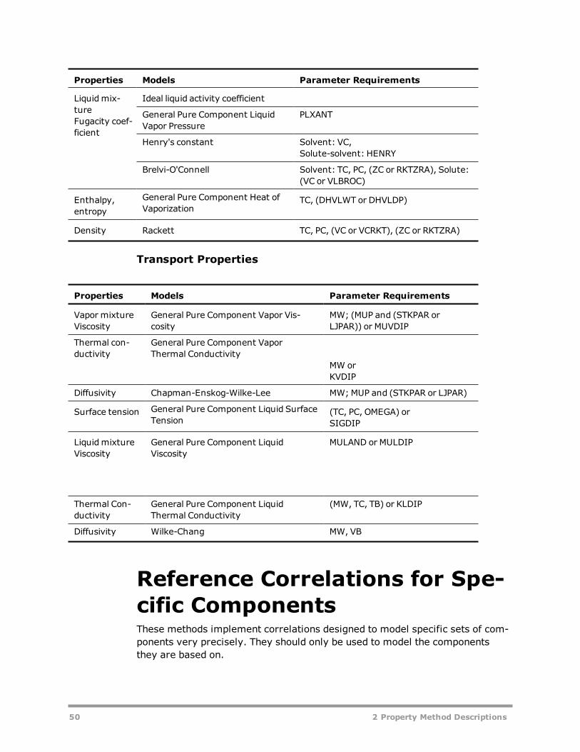
Properties Models Parameter Requirements
Liquidmix-tureFugacity coef-ficient
Ideal liquid activity coefficient
General Pure Component LiquidVapor Pressure
PLXANT
Henry's constant Solvent: VC,Solute-solvent: HENRY
Brelvi-O'Connell Solvent: TC, PC, (ZC or RKTZRA), Solute:(VC or VLBROC)
Enthalpy,entropy
General Pure Component Heat ofVaporization
TC, (DHVLWT or DHVLDP)
Density Rackett TC, PC, (VC or VCRKT), (ZC or RKTZRA)
Transport Properties
Properties Models Parameter Requirements
Vapor mixtureViscosity
General Pure Component Vapor Vis-cosity
MW; (MUP and (STKPAR orLJPAR)) or MUVDIP
Thermal con-ductivity
General Pure Component VaporThermal Conductivity
MW orKVDIP
Diffusivity Chapman-Enskog-Wilke-Lee MW;MUP and (STKPAR or LJPAR)
Surface tension General Pure Component Liquid SurfaceTension
(TC, PC, OMEGA) orSIGDIP
LiquidmixtureViscosity
General Pure Component LiquidViscosity
MULAND or MULDIP
Thermal Con-ductivity
General Pure Component LiquidThermal Conductivity
(MW, TC, TB) or KLDIP
Diffusivity Wilke-Chang MW, VB
Reference Correlations for Spe-cific ComponentsThese methods implement correlations designed to model specific sets of com-ponents very precisely. They should only be used to model the componentsthey are based on.
50 2 Property Method Descriptions

Property Methods for Specific Components
Property Method Model Components
REFPROP NIST Reference Fluid Ther-modynamic and TransportDatabase
Water, natural gas, commonhydrocarbons, and refri-gerants
GERG2008 ISO-20765 (2008 extensionof GERG-2004 equation ofstate)
Natural gas
REFPROP (NIST Reference Fluid Ther-modynamic and Transport Properties Data-base)
OverviewREFPROP is an acronym for REFerence fluid PROPerties. This model, developedby the National Institute of Standards and Technology (NIST), provides ther-modynamic and transport properties of industrially important fluids and theirmixtures with an emphasis on refrigerants and hydrocarbons, especially nat-ural gas systems.
REFPROP is based on the most accurate pure fluid and mixture models currentlyavailable. It implements three models for the thermodynamic properties ofpure fluids: equations of state explicit in Helmholtz energy, the modified Bene-dict-Webb-Rubin equation of state, and an extended corresponding states (ECS)model. Mixture calculations employ a model that applies mixing rules to theHelmholtz energy of the mixture components; it uses a departure function toaccount for the departure from ideal mixing. Viscosity and thermal conductivityare modeled with either fluid-specific correlations, an ECS method, or in somecases the friction theory method.
REFPROP in the Aspen Physical Property System is provided under an agree-ment with the National Institute of Standards and Technology's (NIST) Stand-ard Reference Data Program (SRDP).
Fluids, models, and available propertiesREFPROP in the Aspen Physical Property System includes 120 pure fluids:
l The typical natural gas constituents methane, ethane, propane, butane,isobutane, pentane, isopentane, hexane, isohexane, heptane, octane,isooctane, nonane, decane, undecane, dodecane, carbon dioxide, carbonmonoxide, hydrogen, nitrogen, and water
l The hydrocarbons acetone, benzene, ethylbenzene, butene, cis-butene,cyclohexane, cyclopropane, ethylene, isobutene, neopentane, propyne,
2 Property Method Descriptions 51

trans-butene, toluene, methylcyclohexane, n-propylcyclohexane, cyc-lopentane, m-xylene, o-xylene, and p-xylene
l The HFCs R23, R32, R41, R125, R134a, R143a, R152a, R161, R227ea,R236ea, R236fa, R245ca, R245fa, R365mfc, R1234yf, R1234ze, R-E143a,R-E245cb2, R-E245fa2, R-E347mcc
l The HCFCs R21, R22, R123, R124, R141b, and R142bl The traditional CFCs R11, R12, R13, R113, R114, and R115l The fluorocarbons R14, R116, R218, C4F10, C5F12, RC318, R-1216l The HCC R-40 (methyl chloride)l The "natural" refrigerants ammonia, carbon dioxide, propane, isobutane,and propylene
l The main air constituents nitrogen, oxygen, and argonl The noble elements helium, argon, neon, krypton, and xenonl The cryogens argon, carbon monoxide, deuterium, krypton, neon, nitro-gen trifluoride, nitrogen, fluorine, helium, methane, oxygen, normalhydrogen, parahydrogen, and orthohydrogen
l The fatty acid methyl esters (FAMEs) methyl linoleate, methyl linolen-ate, methyl oleate, methyl palmitate, and methyl stearate
l The siloxanes hexamethyldisiloxane, octamethylcyclotetrasiloxane, octa-methyltrisiloxane, decamethylcyclopentasiloxane, decamethyl-tetrasiloxane, dodecamethylcyclehexasiloxane,dodecamethylpentasiloxane, tetradecamethylhexasiloxane
l Water (as a pure fluid)l Miscellaneous substances including carbonyl sulfide, dimethyl ether,diethyl ether, ethanol, heavy water, hydrogen sulfide, hydrogen chlor-ide, methanol, nitrous oxide, sulfur hexafluoride, sulfur dioxide, tri-fluoroiodomethane, and dimethyl carbonate.
The REFPROP model uses the most accurate equations of state and models cur-rently available:
l High accuracy Helmholtz energy equations of state, including inter-national standard equations for water[1], R134a[2], R32[3], and R143a[4] and equations from the literature for ethane[5], propane[6], R125[7], ammonia[8], carbon dioxide[9], and others
l High accuracy MBWR equations of state, including the international stand-ard EOS for R123[10]
l The Bender equation of state for several of the "older" refrigerants,including R14[11], R114[11], and RC318[11]
l An extended corresponding states model for fluids with limited datal An excess Helmholtz energy model for mixture propertiesl Experimentally based values of the mixture parameters are available forhundreds of mixtures
l Viscosity and thermal conductivity are based on fluid-specific cor-
52 2 Property Method Descriptions

relations (where available), a modification of the extended cor-responding states model, or the friction theory model
Available properties:
l Thermodynamic properties: Density (molar volume), fugacity, Enthalpy,Entropy, Gibbs free energy
l Transport properties: Thermal conductivity, Viscosity, Surface TensionImportant: For components that are not included in the valid REFPROP component list,the Aspen Physical Property System will ignore these components and calculate the phys-ical properties for the remaining components that are on the list. Pure component prop-erties of the non-REFPROP components will be missing. For mixture properties, the molefractions used in the calculations will be re-normalized.
CautionsThe AGA8 equation of state model is not available in the REFPROP model in theAspen Physical Property System. The GERG-2004 model, with its 2008 exten-sions, is available as the separate GERG2008 property method.
Enthalpy, entropy and Gibbs free energy values obtained from Aspen Plus usingREFPROP model are different from those calculated using the standaloneREFPROP program distributed by NIST. This is because of the difference in thereference states used in the two programs. In Aspen Plus, the reference state isideal gas at 298.15 K and 1 atm, while in the standalone REFPROP program[12], [13], the reference states are set up differently. Please see the inform-ation on reference state given below. However, the calculation of the departurefunction of these properties is the same.
The REFPROP model is designed to provide the most accurate thermophysicalproperties currently available for pure fluids and their mixtures. The presentversion is limited to vapor-liquid equilibrium (VLE), liquid-liquid equilibrium(LLE), and vapor-liquid-liquid equilibrium (VLLE). The model does not know thelocation of the freezing line for mixtures. Certain mixtures can potentially enterinto these areas without giving warnings to the user.
Some mixtures have components with a wide range of volatilities, as indicatedby a critical temperature ratio greater than 2. Certain calculations, especiallysaturation calculations, may fail without generating warnings.
Two equations of state are available for hydrogen to account for the differentquantum states of the molecule. These are implemented as two different com-ponents:
l Normal hydrogen should be used in applications where it was createdand stored at 250 K or above, or when it was cooled to below 250 K andstored without a catalyst for less than a day.
l Para hydrogen should be used where hydrogen was catalyzed or storedfor several days at the normal boiling point (NBP) and used at any tem-perature within 1 day of storage at the NBP.
2 Property Method Descriptions 53

Since the rate of conversion between quantum states is dependent on tem-perature, pressure, and the storage container, these values are only estimates.For more information, see the Jacobsen et al. [14] literature reference forhydrogen. Orthohydrogen is also available as a component for use in modelinghydrogen as a mixture of the two different quantum states.
Viscosity and thermal conductivity models are not available for some fluids.Therefore, REFPROP will not be able to return meaningful values for pure ormixture properties of systems that contain one or more of these fluids. Thesefluids are: SO2 (sulfur dioxide), SF6 (sulfur hexafluoride), Propyne, NF3 (nitro-gen trifluoride), Fluorine, Deuterium, cyclopropane, carbonyl sulfide, C5F12(dodecafluoropentane), C4F10 (decafluorobutane), benzene, toluene, acetone,R21 (dichlorofluoromethane), R236ea (1,1,1,2,3,3-hexafluoropropane).
The lower temperature limit for pure Helium is 2.1768 K. Below this tem-perature, Helium is a super-fluid; its properties change dramatically and cannotbe adequately represented by the current model.
Reference stateThe absolute values of enthalpy, entropy, and Gibbs free energy at a singlestate point are meaningless. It is only the difference between two differentstate points that matter. Thus, the value for a single state point can be set toany arbitrary value. Many handbooks set the arbitrary state point so that thevalues of these properties are positive for most liquid or gas states.
In the Aspen Physical Property System, the reference state on which the valuesof the enthalpy and Gibbs free energy are based is:
l Setting enthalpy to the ideal gas enthalpy of formation of the componentat 298.15 K and 1 atm (101325 Pa).
l Setting Gibbs free energy to the ideal gas Gibbs free energy of formationof the component at 298.15 K and 1 atm (101325 Pa).
In the REFPROP standalone program, there are three choices for the referencestate on which the values of enthalpy and entropy are based:
l Setting enthalpy and entropy to zero for the saturated liquid at the nor-mal boiling point (designated as NBP).
l Setting enthalpy and entropy to zero for the saturated liquid at -40 °C(designated as ASHRAE).
l Setting enthalpy to 200 kJ/kg and entropy to 1.0 kJ/(kg-K) for the sat-urated liquid at 0 °C (designated as IIR).
For detailed information on the reference states in Aspen Plus and REFPROPstandalone program, please see help topics for the respective software.
54 2 Property Method Descriptions

Miscellaneous components in REFPROP and the valid tem-perature and pressure ranges
Component name CAS num-ber
Full Chemical Name EOS Temperature andPressure Limits
ACETONE 67-64-1 propanone 178.5-550 K, 700 Mpa
AMMONIA 7664-41-7 ammonia 195.495-700 K, 1000MPa
ARGON 7440-37-1 argon 83.8058-2000 K,1000MPa
CARBON-DIOXIDE 124-38-9 carbon dioxide 216.592-2000 K, 800MPa
CARBON-MONOXIDE 630-08-0 carbon monoxide 68.16-500 K, 100 MPa
CARBONYL-SULFIDE 463-58-1 carbon oxide sulfide 134.3-650 K, 50 MPa
DEUTERIUM 7782-39-0 deuterium 18.71-423 K, 320 Mpa
DIETHYL-ETHER 60-29-7 diethyl ether 270-500 K, 40 MPa
DIMETHYL-CARBONATE 616-38-6 dimethyl ester carbonic acid 277.06-400 K, 60 MPa
DIMETHYL-ETHER 115-10-6 ethylene oxide 131.65-525 K, 40 MPa
ETHANOL 64-17-5 ethyl alcohol 250-650 K, 280 MPa
FLUORINE 7782-41-4 fluorine 53.4811-300 K, 20 MPa
DEUTERIUM-OXIDE 7789-20-0 deuterium oxide 276.97-800 K, 100 MPa
HELIUM-4 7440-59-7 helium-4 2.1768**-1500 K, 100MPa
HYDROGEN 1333-74-0 hydrogen (normal) 13.957-1000 K, 2000MPa
HYDROGEN-PARA parahydrogen 13.803-1000 K, 2000MPa
HYDROGEN,-DIATOMIC,-ORTHO
999989-91-2
orthohydrogen 14.008-1000 K, 2000MPa
HYDROGEN-CHLORIDE 7647-01-0 hydrogen chloride 155-330 K, 20 MPa
HYDROGEN-SULFIDE 7783-06-4 hydrogen sulfide 187.7-760 K, 170 MPa
KRYPTON 7439-90-9 krypton 115.775-750 K, 200 MPa
METHANOL 67-56-1 methanol 175.61-620 K, 800 MPa
NEON 7440-01-9 neon 24.556-700 K, 700 MPa
2 Property Method Descriptions 55
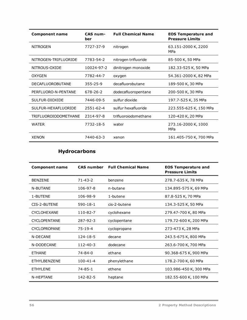
Component name CAS num-ber
Full Chemical Name EOS Temperature andPressure Limits
NITROGEN 7727-37-9 nitrogen 63.151-2000 K, 2200MPa
NITROGEN-TRIFLUORIDE 7783-54-2 nitrogen trifluoride 85-500 K, 50 MPa
NITROUS-OXIDE 10024-97-2 dinitrogen monoxide 182.33-525 K, 50 MPa
OXYGEN 7782-44-7 oxygen 54.361-2000 K, 82 MPa
DECAFLUOROBUTANE 355-25-9 decafluorobutane 189-500 K, 30 MPa
PERFLUORO-N-PENTANE 678-26-2 dodecafluoropentane 200-500 K, 30 MPa
SULFUR-DIOXIDE 7446-09-5 sulfur dioxide 197.7-525 K, 35 MPa
SULFUR-HEXAFLUORIDE 2551-62-4 sulfur hexafluoride 223.555-625 K, 150 MPa
TRIFLUOROIODOMETHANE 2314-97-8 trifluoroiodomethane 120-420 K, 20 MPa
WATER 7732-18-5 water 273.16-2000 K, 1000MPa
XENON 7440-63-3 xenon 161.405-750 K, 700 MPa
Hydrocarbons
Component name CAS number Full Chemical Name EOS Temperature andPressure Limits
BENZENE 71-43-2 benzene 278.7-635 K, 78 MPa
N-BUTANE 106-97-8 n-butane 134.895-575 K, 69 MPa
1-BUTENE 106-98-9 1-butene 87.8-525 K, 70 MPa
CIS-2-BUTENE 590-18-1 cis-2-butene 134.3-525 K, 50 MPa
CYCLOHEXANE 110-82-7 cyclohexane 279.47-700 K, 80 MPa
CYCLOPENTANE 287-92-3 cyclopentane 179.72-600 K, 200 MPa
CYCLOPROPANE 75-19-4 cyclopropane 273-473 K, 28 MPa
N-DECANE 124-18-5 decane 243.5-675 K, 800 MPa
N-DODECANE 112-40-3 dodecane 263.6-700 K, 700 MPa
ETHANE 74-84-0 ethane 90.368-675 K, 900 MPa
ETHYLBENZENE 100-41-4 phenylethane 178.2-700 K, 60 MPa
ETHYLENE 74-85-1 ethene 103.986-450 K, 300 MPa
N-HEPTANE 142-82-5 heptane 182.55-600 K, 100 MPa
56 2 Property Method Descriptions

Component name CAS number Full Chemical Name EOS Temperature andPressure Limits
N-HEXANE 110-54-3 hexane 177.83-600 K, 100 MPa
ISOBUTANE 75-28-5 2-methylpropane 113.73-575 K, 35 MPa
ISOBUTYLENE 115-11-7 2-methyl-1-propene 132.4-550 K, 50 MPa
2,2,4-TRIMETHYLPENTANE
540-84-1 isooctane 165.77-600 K, 1000 MPa
2-METHYL-PENTANE 107-83-5 2-methylpentane 119.6-550 K, 1000 MPa
2-METHYL-BUTANE 78-78-4 2-methylbutane 112.65-500 K, 1000 MPa
METHANE 74-82-8 methane 90.6941-625 K, 1000 MPa
METHYLCYCLOHEXANE 108-87-2 methylcyclohexane 146.7-600 K, 500 MPa
2,2-DIMETHYL-PROPANE
463-82-1 2,2-dimethylpropane 256.6-550 K, 200 MPa
N-NONANE 111-84-2 nonane 219.7-600 K, 800 MPa
N-OCTANE 111-65-9 octane 216.37-600 K, 100 MPa
N-PENTANE 109-66-0 pentane 143.47-600 K, 100 MPa
PROPANE 74-98-6 propane 85.53-625 K, 1000 MPa
N-PROPYLCYCLOHEXANE
1678-92-8 n-propylcyclohexane 178.2-650 K, 50 MPa
PROPYLENE 115-07-1 propene 87.953-575 K, 1000 MPa
METHYL-ACETYLENE 74-99-7 propyne 273-474 K, 32 MPa
TOLUENE 108-88-3 methylbenzene 178-700 K, 500 MPa
TRANS-2-BUTENE 624-64-6 trans-2-butene 167.6-525 K, 50 MPa
N-UNDECANE 1120-21-4 undecane 247.541-700 K, 500 MPa
M-XYLENE 108-38-3 1,3-methylbenzene 225.3-700 K, 200 MPa
O-XYLENE 95-47-6 1,2-methylbenzene 247.985-700 K, 70 MPa
P-XYLENE 106-42-3 1,4-methylbenzene 286.4-700 K, 200 MPa
Fatty Acid Methyl Esters
Component name CAS num-ber
Full Chemical Name EOS Temperature andPressure Limits
METHYL-LINOLEATE 112-63-0 methyl (Z,Z)-9,12-oct-adecadienoate
238.1-1000 K, 50 MPa
2 Property Method Descriptions 57

Component name CAS num-ber
Full Chemical Name EOS Temperature andPressure Limits
METHYL-LINOLENATE 301-00-8 methyl (Z,Z,Z)-9,12,15-oct-adecatrienoate
218.65-1000 K, 50 MPa
METHYL-OLEATE 112-62-9 methyl cis-9-octadecenoate 253.47-1000 K, 50 MPa
METHYL-PALMITATE 112-39-0 methyl hexadecanoate 242-1000 K, 50 MPa
METHYL-STEARATE 112-61-8 methyl octadecanoate 311.4- 1000 K, 50 MPa
Siloxanes
Component name CAS number EOS Temperature and PressureLimits
HEXAMETHYLDISILOXANE 107-46-0 273-673 K, 30 MPa
OCTAMETHYLCYCLOTETRASILOXANE 556-67-2 300-673 K, 30 MPa
OCTAMETHYLTRISILOXANE 107-51-7 187.2-673 K, 30 MPa
DECAMETHYLCYCLOPENTASILOXANE 541-02-6 300-673 K, 30 MPa
DECAMETHYLTETRASILOXANE 141-62-8 205.2-673 K, 30 MPa
DODECAMETHYLCYCLOHEXASILOXANE 540-97-6 270.2-673 K, 30 MPa
DODECAMETHYLPENTASILOXANE 141-63-9 192-673 K, 30 MPa
TETRADECAMETHYLHEXASILOXANE 107-52-8 300-673 K, 30 MPa
Refrigerants
Component name CAS num-ber
Refrigerantname
EOS Temperature andPressure Limits
TRICHLOROFLUOROMETHANE 75-69-4 R11 162.68-625 K, 30 MPa
DICHLORODIFLUOROMETHANE 75-71-8 R12 116.099-525 K, 200 MPa
CHLOROTRIFLUOROMETHANE 75-72-9 R13 92-403 K, 35 MPa
CARBON-TETRAFLUORIDE 75-73-0 R14 120-623 K, 51 MPa
DICHLOROMONOFLUOROMETHANE 75-43-4 R21 200-473 K, 138 MPa
CHLORODIFLUOROMETHANE 75-45-6 R22 115.73-550 K, 60 MPa
TRIFLUOROMETHANE 75-46-7 R23 118.02-475 K, 120 MPa
DIFLUOROMETHANE 75-10-5 R32 136.34-435 K, 70 MPa
58 2 Property Method Descriptions

Component name CAS num-ber
Refrigerantname
EOS Temperature andPressure Limits
METHYL-CHLORIDE 74-87-3 R40 230-630 K, 100 MPa
METHYL-FLUORIDE 593-53-3 R41 129.82-425 K, 70 MPa
1,2,2-TRICHLORO-1,1,2-TRIFLUOROE 76-13-1 R113 236.93-525 K, 200 MPa
1,2-DICHLORO-1,1,2,2-TETRAFLUORO
76-14-2 R114 273.15-507 K, 21 MPa
CHLOROPENTAFLUOROETHANE 76-15-3 R115 173.75-550 K, 60 MPa
PERFLUOROETHANE 76-16-4 R116 173.1-425 K, 50 MPa
1,1-DICHLORO-2,2,2-TRIFLUOROETHA
306-83-2 R123 166-600 K, 40 MPa
HFO-1234YF 754-12-1 R1234yf 220-410 K, 30 MPa
TRANS-1,3,3,3-TETRAFLUORPROPENE 29118-24-9 R1234ze 168.62-420 K, 20 MPa
2-CHLORO-1,1,1,2-TETRAFLUOROETHA
2837-89-0 R124 120-470 K, 40 MPa
PENTAFLUOROETHANE 354-33-6 R125 172.52-500 K, 60 MPa
1,1,1,2-TETRAFLUOROETHANE 811-97-2 R134a 169.85-455 K, 70 MPa
1,1-DICHLORO-1-FLUOROETHANE 1717-00-6 R141b 169.68-500 K, 400 MPa
1-CHLORO-1,1-DIFLUOROETHANE 75-68-3 R142b 142.72-470 K, 60 MPa
1,1,1-TRIFLUOROETHANE 420-46-2 R143a 161.34-650 K, 100 MPa
1,1-DIFLUOROETHANE 75-37-6 R152a 154.56-500 K, 60 MPa
ETHYL-FLUORIDE 353-36-6 R161 130-400 K, 50 MPa
OCTAFLUOROPROPANE 76-19-7 R218 125.45-440 K, 20 MPa
1,1,1,2,3,3,3-HEPTAFLUOROPROPANE 431-89-0 R227ea 146.35-475 K, 60 MPa
1,1,1,2,3,3-HEXAFLUOROPROPANE 431-63-0 R236ea 242-500 K, 60 MPa
*HFC-236FA 690-39-1 R236fa 179.52-500 K, 40 MPa
1,1,2,2,3-PENTAFLUOROPROPANE 679-86-7 R245ca 200-500 K, 60 MPa
1,1,1,3,3-PENTAFLUOROPROPANE 460-73-1 R245fa 171.05-440 K, 200 MPa
*1,1,1,3,3-PENTAFLUOROBUTANE 406-58-6 R365mfc 239-500 K, 35 MPa
HEXAFLUOROPROPYLENE 116-15-4 R1216 117.654-400 K, 12 MPa
OCTAFLUOROCYCLOBUTANE 115-25-3 RC318 233.35-623 K, 60 MPa
2 Property Method Descriptions 59

Component name CAS num-ber
Refrigerantname
EOS Temperature andPressure Limits
METHYL-TRIFLUOROMETHYL-ETHER 421-14-7 RE143a 240-420 K, 7.2 MPa
PENTAFLUOROETHYL-METHYL-ETHER 22410-44-2 RE245cb2 250-500 K, 20 MPa
2-DIFLUOROMETHOXY-1,1,1-TRIFLURO
1885-48-9 RE245fa2 250-500 K, 400 MPa
HEPTAFLUOROPROPYL-METHYL-ETHER
375-03-1 RE347mcc 250-500 K, 20 MPa
* Component only available in NIST database.
** Although the lower limit of applicability for the helium model is 2.1768 K, theglobal flash temperature lower limit is by default 10 K. To perform calculationswith helium below 10 K, change the Lower limit for Temperature on theSetup | Calculation Options | Flash Convergence sheet. If using AspenProperties within another program, this default needs to be set in Aspen Prop-erties while configuring properties for that program.
References[1] Wagner W., Pruss A., "The IAPWS Formulation 1995 for the ThermodynamicProperties of Ordinary Water Substance for General and Scientific Use" J. Phys.Chem. Ref.Data, 2002, Vol. 31, No. 2, 387-535
[2] Tillner-Roth, R. and Baehr, H.D., "An international standard formulation ofthe thermodynamic properties of 1,1,1,2-tetrafluoroethane (HFC-134a) for tem-peratures from 170 K to 455 K at pressures up to 70 MPa," J. Phys. Chem. Ref.Data, 1994, Vol. 23, 657-729
[3] Tillner-Roth, R. and Yokozeki, A.,"An international standard equation ofstate for difluoromethane (R-32) for temperatures from the triple point at136.34 K to 435 K and pressures up to 70 MPa," J. Phys. Chem. Ref. Data, 1997,Vol. 25, No. 6, 1273-1328
[4] Lemmon, E.W. and Jacobsen, R.T,"An International Standard Formulationfor the Thermodynamic Properties of 1,1,1-Trifluoroethane (HFC-143a) for Tem-peratures from 161 to 450 K and Pressures to 50 MPa," J. Phys. Chem. Ref.Data, 2000, Vol. 29, No. 4, 521-552
[5] Buecker, D. and Wagner, W. "A Reference Equation of State for the Ther-modynamic Properties of Ethane for Temperatures from the Melting Line to 675K and Pressures up to 900 MPa," J. Phys. Chem. Ref. Data, 2006, Vol. 35, No. 1,205-266
[6] Lemmon, E.W., McLinden, M.O., Wagner, W. to be submitted to J. Phys.Chem. Ref. Data, 2007.
60 2 Property Method Descriptions

[7] Lemmon, E.W. and Jacobsen, R.T, "A New Functional Form and New FittingTechniques for Equations of State with Application to Pentafluoroethane (HFC-125)," J. Phys. Chem. Ref. Data, 2005, Vol. 34, No. 1, 69-108
[8] Tillner-Roth, R., Harms-Watzenberg, F., and Baehr, H.D., "Eine neue Fun-damentalgleichung fuer Ammoniak," DKV-Tagungsbericht, 1993, Vol. 20, 167-181
[9] Span, R. and Wagner, W., "A New Equation of State for Carbon DioxideCovering the Fluid Region from the Triple-Point Temperature to 1100 K at Pres-sures up to 800 MPa," J. Phys. Chem. Ref. Data, 1996, Vol. 25, No. 6, 1509-1596
[10] Younglove, B.A. and McLinden, M.O., "An International Standard Equationof State for the Thermodynamic Properties of Refrigerant 123 (2,2-Dichloro-1,1,1-trifluoroethane)," J. Phys. Chem. Ref. Data, 1994, Vol. 23, 731-779
[11] Platzer, B., Polt, A., and Maurer, G., "Thermophysical properties of refri-gerants," Berlin: Springer-Verlag, 1990.
[12] Lemmon E.W., Huber M.L., McLinden M.O. NIST Standard Reference Data-base 23: Reference Fluid Thermodynamic and Transport Properties-REFPROP,Version 8.0, National Institute of Standards and Technology, Standard Refer-ence Data Program, Gaithersburg, 2007.
[13] NIST REFPROP website:
[14] Jacobsen R.T., Leachman J.W., Penoncello S.G., Lemmon E.W. "CurrentStatus of Thermodynamic Properties of Hydrogen," International Journal ofThermophysics, 2007, Vol. 28, No. 3, 758-772
GERG2008 Property MethodThe GERG2008 property method is based on the 2008 extension of the GERG-2004 equation of state model for calculations of thermodynamic properties andphase equilibrium of natural gases and other mixtures consisting of natural gascomponents.
This model was developed under the auspices of the Groupe Européen deRecherches Gazières (GERG) in cooperation with the German technical andScientific Association on Gas and Water and European natural gas companies(E.ON Ruhrgas, Germany; Enagas, Spain; Gasunie, The Netherlands; Gaz deFrance, France; Snam Rete Gas, Italy; and Statoil, Norway).
This is a highly accurate, wide-range equation of state that has been adopted asa standard (ISO-20765) international reference equation suitable for all naturalgas applications, including processing, transportation, and storage of naturalgas. The model is applicable to 21 natural gas components and their mixtures,including Methane, Nitrogen, Carbon dioxide, Ethane, Propane, n-Butane, Isobu-tane, n-Pentane, Isopentane, n-Hexane, n-Heptane, n-Octane, n-Nonane, n-Decane, Hydrogen, Oxygen, Carbon monoxide, Water, Helium, Argon, and
2 Property Method Descriptions 61
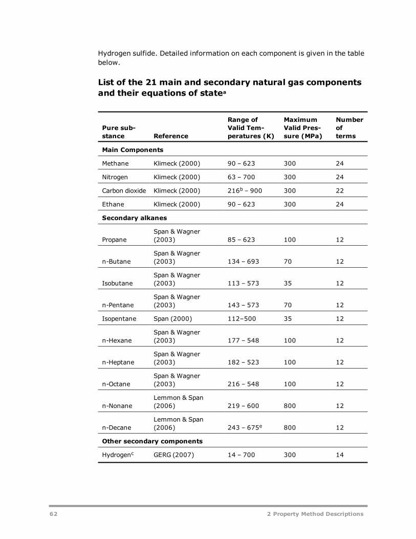
Hydrogen sulfide. Detailed information on each component is given in the tablebelow.
List of the 21 main and secondary natural gas componentsand their equations of statea
Pure sub-stance Reference
Range ofValid Tem-peratures (K)
MaximumValid Pres-sure (MPa)
Numberofterms
Main Components
Methane Klimeck (2000) 90 – 623 300 24
Nitrogen Klimeck (2000) 63 – 700 300 24
Carbon dioxide Klimeck (2000) 216b – 900 300 22
Ethane Klimeck (2000) 90 – 623 300 24
Secondary alkanes
PropaneSpan & Wagner(2003) 85 – 623 100 12
n-ButaneSpan & Wagner(2003) 134 – 693 70 12
IsobutaneSpan & Wagner(2003) 113 – 573 35 12
n-PentaneSpan & Wagner(2003) 143 – 573 70 12
Isopentane Span (2000) 112–500 35 12
n-HexaneSpan & Wagner(2003) 177 – 548 100 12
n-HeptaneSpan & Wagner(2003) 182 – 523 100 12
n-OctaneSpan & Wagner(2003) 216 – 548 100 12
n-NonaneLemmon & Span(2006) 219 – 600 800 12
n-DecaneLemmon & Span(2006) 243 – 675e 800 12
Other secondary components
Hydrogenc GERG (2007) 14 – 700 300 14
62 2 Property Method Descriptions
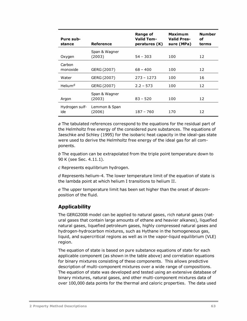
Pure sub-stance Reference
Range ofValid Tem-peratures (K)
MaximumValid Pres-sure (MPa)
Numberofterms
OxygenSpan & Wagner(2003) 54 – 303 100 12
Carbonmonoxide GERG (2007) 68 – 400 100 12
Water GERG (2007) 273 – 1273 100 16
Heliumd GERG (2007) 2.2 – 573 100 12
ArgonSpan & Wagner(2003) 83 – 520 100 12
Hydrogen sulf-ide
Lemmon & Span(2006) 187 – 760 170 12
a The tabulated references correspond to the equations for the residual part ofthe Helmholtz free energy of the considered pure substances. The equations ofJaeschke and Schley (1995) for the isobaric heat capacity in the ideal-gas statewere used to derive the Helmholtz free energy of the ideal gas for all com-ponents.
b The equation can be extrapolated from the triple point temperature down to90 K (see Sec. 4.11.1).
c Represents equilibrium hydrogen.
d Represents helium-4. The lower temperature limit of the equation of state isthe lambda point at which helium I transitions to helium II.
e The upper temperature limit has been set higher than the onset of decom-position of the fluid.
ApplicabilityThe GERG2008 model can be applied to natural gases, rich natural gases (nat-ural gases that contain large amounts of ethane and heavier alkanes), liquefiednatural gases, liquefied petroleum gases, highly compressed natural gases andhydrogen-hydrocarbon mixtures, such as Hythane in the homogeneous gas,liquid, and supercritical regions as well as in the vapor-liquid equilibrium (VLE)region.
The equation of state is based on pure substance equations of state for eachapplicable component (as shown in the table above) and correlation equationsfor binary mixtures consisting of these components. This allows predictivedescription of multi-component mixtures over a wide range of compositions.The equation of state was developed and tested using an extensive database ofbinary mixtures, natural gases, and other multi-component mixtures data ofover 100,000 data points for the thermal and caloric properties. The data used
2 Property Method Descriptions 63

cover the homogeneous gas, liquid, and supercritical regions as well as vapor-liquid equilibrium (VLE) states. The types of data used include: PVT, isochoricheat capacity (Cv), speed of sound (w), isobaric heat capacity (Cp), enthalpydifference, excess molar enthalpy, saturated liquid density, and VLE data.About 75% of the data are for binary mixtures, while the remaining 25% are formulti-component mixtures. Almost 70% of the mixture data describe a PVTrelation, more than 20% of the data are vapor-liquid equilibrium state points,and less than 10% account for caloric properties. About 50% of the availablebinary mixture data were used for model development while the remainingdata were used for model validation.
The model cannot be used for components other than the ones listed above.
The GERG2008 model is available in Aspen Plus through the RefProp programdeveloped by the National Institute of Standards and Technology (NIST).
Range of Validity and Estimates of UncertaintyThe GERG2008 model is valid in the homogeneous gas, liquid, and supercriticalregions and in the vapor-liquid states. Due to the vast amount of experimentaldata for the different binary and multi-component mixtures, and the varyingreal mixture behavior, which strongly depends on temperature, pressure andcomposition, it is impossible to discuss each binary and multi-component sys-tem separately. In general, there are no restrictions concerning the com-position range, but the uncertainty is mostly unknown for the compositionranges not covered by the experimental data.
The range of validity of the model related to the calculation of thermal and cal-oric properties of mixtures is divided into three parts: the normal range and theextended range.
In the normal range, the validity covers temperatures of 90 K ≤ T ≤ 450 K andpressures of p ≤ 35 MPa. This range corresponds to the use of the equation inapplications using natural gas and related mixtures in pipeline transport, nat-ural gas storage, and improved processes with liquefied natural gas.
The uncertainty for the important properties and phases are as follow:
l The uncertainty in gas phase density is < 0.1% for the temperaturerange from 250 – 450 K and pressure up to 35 MPa for various types ofnatural gases, including natural gases rich in nitrogen, rich in carbondioxide, rich in ethane, rich in hydrogen, and natural gases containingconsiderable amounts of propane, and heavier alkanes, carbon monox-ide, or oxygen and other mixtures consisting of the 21 natural gas com-ponents. The great majority of experimental densities for various richnatural gases containing large amounts of carbon dioxide (up to 20%),ethane (up to 18%), propane (up to 14%), n-butane (up to 6%), n-pentane (up to 0.5%), and n-hexane (0.2%) are reproduced to within ±(0.1 – 0.3)% over the temperature range 280 K to 350 K and pressure upto 30 MPa.
l The uncertainty in gas phase speed of sound is < 0.1% in the
64 2 Property Method Descriptions

temperature range from 270 K to 450 K and pressures up to 20 MPa, andin the temperature range from 250 K to 270 K at pressures up to 12 MPa.At higher pressures, the uncertainty is < (0.2 – 0.3)%.
l The uncertainty in gas phase isobaric enthalpy difference is < (0.2 –0.5)%.
l The uncertainty for isobaric and isochoric heat capacity (Cp and Cv,respectively) in the homogeneous gas, liquid, and supercritical regions is±(1 – 2)%
l The uncertainty for liquid phase isobaric enthalpy difference is ± (0.5 –1)%.
l The uncertainty in liquid phase density is ±(0.1 – 0.5)%.for pressuresup to 40 MPa for many binary and multi-component mixtures, includingLNG-like mixtures and mixtures of light and heavy hydrocarbons.
l The uncertainty for saturated liquid density for the same types of mix-tures in the temperate range from 100 K to 140 K, which is very import-ant for processes with liquefied natural gas, is < (0.1 – 0.3)%.
l Vapor-liquid equilibrium data of binary and multi-component mixtures aswell as dew points of natural gases and hydrocarbon mixtures are accur-ately described. The most accurate vapor pressure data for binary andternary mixtures consisting of the natural gas main components (meth-ane, nitrogen, carbon dioxide, and ethane), as well as propane, n-butaneand isobutene are reproduced to within their experimental uncertainty(~ (1-3)%). Certain other mixtures have higher uncertainty of up to 5%or more. Accurate experimental vapor phase compositions aredescribed to within ±(0.5 – 1) mole %.
The extended range of validity covers temperatures of 60 K ≤ T ≤ 700 K andpressures of p ≤ 70 MPa and has the following uncertainty:
l The uncertainty of gas phase density is (0.2 – 0.5)% at temperaturesand pressures outside the normal range of validity
l Density data of certain binary mixtures are described to within ±(0.5 –1)% at pressures up to 100 MPa or more.
l The current data situation outside the normal range does not allow forwell-founded estimates of uncertainty of other thermodynamic prop-erties.
ReferencesKlimeck, R. "Entwicklung einer Fundamentalgleichung für Erdgase für das Gas-und Flüssigkeitsgebiet sowie das Phasengleichgewicht." Dissertation, Fakultätfür Maschinenbau, Ruhr-Universität Bochum, 2000.
Span, R. "A simultaneously optimised equation of state for isopentane." Privatecommunication, Lehrstuhl für Thermodynamik, Ruhr-Universität Bochum, 2000.
Span, R.; Wagner, W. "Equations of state for technical applications. II. Resultsfor nonpolar fluids." Int. J. Thermophysics, 24 (2003), 41–109.
2 Property Method Descriptions 65

Lemmon, E. W.; Span, R. "Short fundamental equations of state for 20 indus-trial fluids." J. Chem. Eng. Data, 51 (2006), 785–850.
"The GERG-2004 Wide-Range Equation of State for Natural Gases and Other Mix-tures." O. Kunz, R. Klimeck, W. Wagner, M. Jaeschke; GERG TM15 2007; ISBN978-3-18-355706-6; Published for GERG and printed in Germany by VDI VerlagGmbH (2007).
Property Methods for PetroleumMixturesThe property methods in the following table are designed for mixtures of hydro-carbons and light gases. K-value models and liquid fugacity correlations areused at low and medium pressures. Petroleum-tuned equations of state areused at high pressures. The hydrocarbons can be from natural gas or crude oil:that is, complex mixtures that are treated using pseudocomponents. Theseproperty methods are often used for refinery applications. Density and trans-port properties are calculated by API procedures when possible.
The following table lists the common and the distinctive models of the propertymethods. The parameter requirements of the distinctive models are given inthe tables labeled Parameters Required for the CHAO-SEA Property Method(see CHAO-SEA), Parameters Required for the GRAYSON Property Method (seeGRAYSON), Parameters Required for the PENG-ROB Property Method (seePENG-ROB), and Parameters Required for the RK-SOAVE Property Method (seeRK-SOAVE).
Parameter requirements for the common models are in the table labeled Para-meters Required for Common Models. For details on these models, see PhysicalProperty Models.
Property Methods for Petroleum Mixtures
Liquid Fugacity and K-Value Models
Property Method Name Models
BK10 Braun K10 K-value model
CHAO-SEA Chao-Seader liquid fugacity, Scatchard-Hildebrand activity coefficient
GRAYSON/GRAYSON2 Grayson-Streed liquid fugacity, Scatchard-Hildebrand activity coefficient
MXBONNEL Maxwell-Bonnell liquid fugacity
66 2 Property Method Descriptions
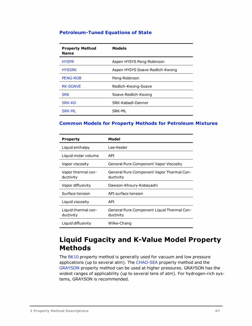
Petroleum-Tuned Equations of State
Property MethodName
Models
HYSPR Aspen HYSYS Peng-Robinson
HYSSRK Aspen HYSYS Soave-Redlich-Kwong
PENG-ROB Peng-Robinson
RK-SOAVE Redlich-Kwong-Soave
SRK Soave-Redlich-Kwong
SRK-KD SRK-Kabadi-Danner
SRK-ML SRK-ML
Common Models for Property Methods for Petroleum Mixtures
Property Model
Liquid enthalpy Lee-Kesler
Liquidmolar volume API
Vapor viscosity General Pure Component Vapor Viscosity
Vapor thermal con-ductivity
General Pure Component Vapor Thermal Con-ductivity
Vapor diffusivity Dawson-Khoury-Kobayashi
Surface tension API surface tension
Liquid viscosity API
Liquid thermal con-ductivity
General Pure Component Liquid Thermal Con-ductivity
Liquid diffusivity Wilke-Chang
Liquid Fugacity and K-Value Model PropertyMethodsThe BK10 property method is generally used for vacuum and low pressureapplications (up to several atm). The CHAO-SEA property method and theGRAYSON property method can be used at higher pressures. GRAYSON has thewidest ranges of applicability (up to several tens of atm). For hydrogen-rich sys-tems, GRAYSON is recommended.
2 Property Method Descriptions 67

These property methods are less suited for high-pressure applications inrefinery (above about 50 atm). Petroleum-tuned equation of state propertymethods are preferred for high pressures.
These property methods are not suited for conditions close to criticality, asoccur in light oil reservoirs, transportation of gas by pipelines, and in some gasprocessing applications. Standard equations of state for non-polar componentsare preferred. If polar compounds are present, such as in gas treatment, useflexible and predictive equations of state for polar compounds.
BK10The BK10 property method uses the Braun K-10 K-value correlations. The cor-relations were developed from the K10 charts for both real components and oilfractions. The real components include 70 hydrocarbons and light gases. The oilfractions cover boiling ranges 450 – 700 K (350 – 800°F). Proprietary methodswere developed to cover heavier oil fractions.
Mixture TypesBest results are obtained with purely aliphatic or purely aromatic mixtures withnormal boiling points ranging from 450 to 700 K. For mixtures of aliphatic andaromatic components, or naphtenic mixtures, the accuracy decreases. For mix-tures with light gases, and medium pressures, CHAO-SEA or GRAYSON arerecommended.
RangeThe BK10 property method is suited for vacuum and low pressure applications(up to several atm). For high pressures, petroleum-tuned equations of state arebest suited.
The applicable temperature range of the K10 chart is 133 – 800 K (-220 –980°F). It can be used up to 1100 K (1520°F).
The parameters for the Braun K-10 are all built-in. You do not need to supplythem. See Parameters Required for Common Models for parameter require-ments of models common to petroleum property methods.
CHAO-SEAThe CHAO-SEA property method uses the:
l Chao-Seader correlation for reference state fugacity coefficientl Scatchard-Hildebrand model for activity coefficientl Redlich-Kwong equation of state for vapor phase propertiesl Lee-Kesler equation of state for liquid and vapor enthalpyl API method for liquid molar volume, viscosity and surface tensionl Models listed in the tables labeled Parameters Required for the CHAO-
68 2 Property Method Descriptions

SEA Property Method (see below), and Parameters Required for Com-mon Models
The tables labeled Parameters Required for the CHAO-SEA Property Method andParameters Required for Common Models provide thermodynamic and trans-port property models, and their parameter requirements.
The CHAO-SEA property method is predictive. It can be used for crude towers,vacuum towers, and some parts of the ethylene process. It is not recom-mended for systems containing hydrogen.
Mixture TypesThe CHAO-SEA property method was developed for systems containing hydro-carbons and light gases, such as carbon dioxide and hydrogen sulfide, but withthe exception of hydrogen. If the system contains hydrogen, use the GRAYSONproperty method.
RangeUse the CHAO-SEA property method for systems with temperature and pres-sure limits of:
200 < T < 533 K
0.5 < Tri < 1.3
Trm < 0.93
P < 140 atm
Where:
Tri = Reduced temperature of a component
Trm = Reduced temperature of the mixture
Do not use this property method at very high pressures, especially near the mix-ture critical point, because of anomalous behavior in these regions.
Parameters Required for the CHAO-SEA Property Method
ThermodynamicProperties
Models Parameter Require-ments
Vapor mixtureFugacity coefficient,Density
Redlich-Kwong TC, PC
2 Property Method Descriptions 69
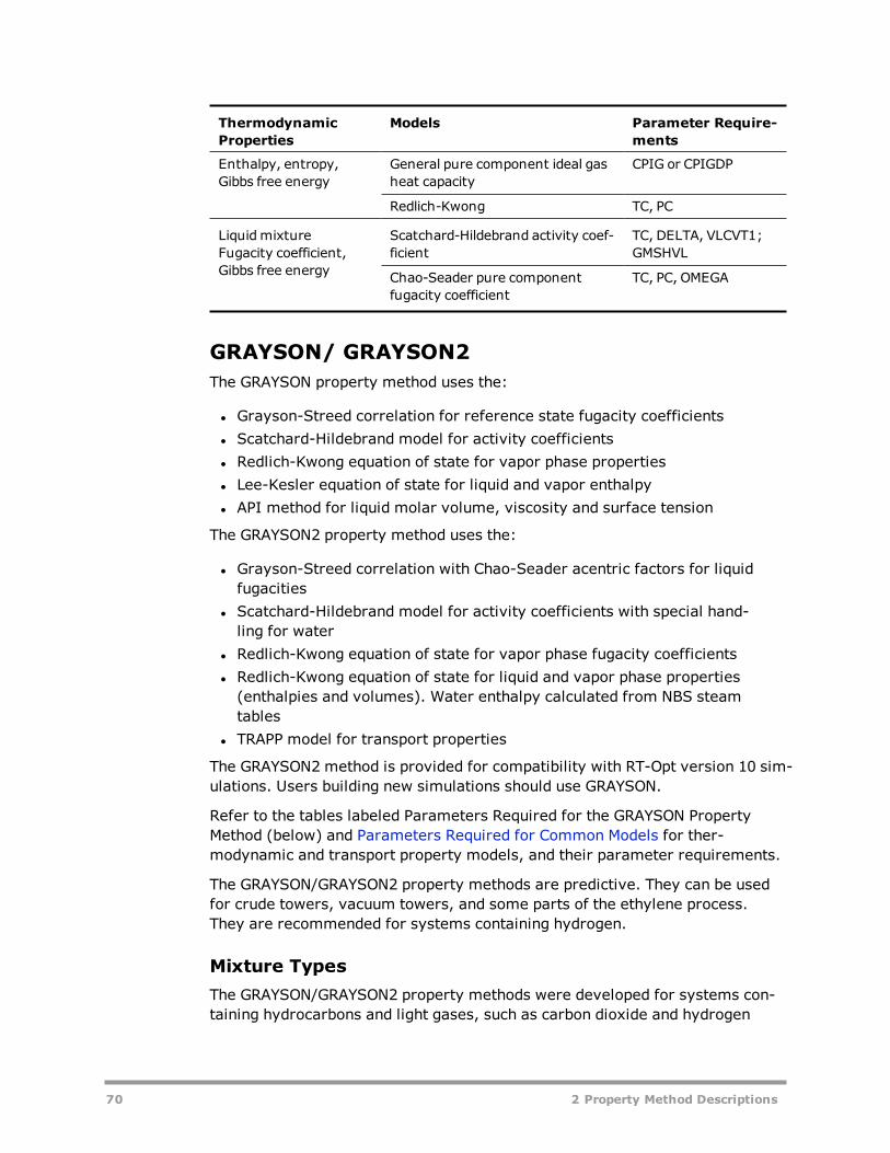
ThermodynamicProperties
Models Parameter Require-ments
Enthalpy, entropy,Gibbs free energy
General pure component ideal gasheat capacity
CPIG or CPIGDP
Redlich-Kwong TC, PC
LiquidmixtureFugacity coefficient,Gibbs free energy
Scatchard-Hildebrand activity coef-ficient
TC, DELTA, VLCVT1;GMSHVL
Chao-Seader pure componentfugacity coefficient
TC, PC, OMEGA
GRAYSON/ GRAYSON2The GRAYSON property method uses the:
l Grayson-Streed correlation for reference state fugacity coefficientsl Scatchard-Hildebrand model for activity coefficientsl Redlich-Kwong equation of state for vapor phase propertiesl Lee-Kesler equation of state for liquid and vapor enthalpyl API method for liquid molar volume, viscosity and surface tension
The GRAYSON2 property method uses the:
l Grayson-Streed correlation with Chao-Seader acentric factors for liquidfugacities
l Scatchard-Hildebrand model for activity coefficients with special hand-ling for water
l Redlich-Kwong equation of state for vapor phase fugacity coefficientsl Redlich-Kwong equation of state for liquid and vapor phase properties(enthalpies and volumes). Water enthalpy calculated from NBS steamtables
l TRAPP model for transport properties
The GRAYSON2 method is provided for compatibility with RT-Opt version 10 sim-ulations. Users building new simulations should use GRAYSON.
Refer to the tables labeled Parameters Required for the GRAYSON PropertyMethod (below) and Parameters Required for Common Models for ther-modynamic and transport property models, and their parameter requirements.
The GRAYSON/GRAYSON2 property methods are predictive. They can be usedfor crude towers, vacuum towers, and some parts of the ethylene process.They are recommended for systems containing hydrogen.
Mixture TypesThe GRAYSON/GRAYSON2 property methods were developed for systems con-taining hydrocarbons and light gases, such as carbon dioxide and hydrogen
70 2 Property Method Descriptions

sulfide. They are recommended over the CHAO-SEA property method when thesystem contains hydrogen.
RangeThe GRAYSON/GRAYSON2 property methods should give reasonable results fortemperatures from 60° F to 800° F for pressures up to 3000 psia. They shouldbe used with caution at pressures above 600 psia and temperatures below 60°F. These methods are not recommended for modeling separations of close-boil-ing components (e.g. isomers). Do not use these property methods at very highpressures, especially near the mixture critical point, because of anomalousbehavior in these regions.
Parameters Required for the GRAYSON Property Method
ThermodynamicProperties
Models Parameter Require-ments
Vapor mixtureFugacity coefficient,Density
Redlich-Kwong TC, PC
Enthalpy, entropy,Gibbs free energy
General pure component ideal gasheat capacity
CPIG or CPIGDP
Redlich-Kwong TC, PC
LiquidmixtureFugacity coefficient,Gibbs free energy
Scatchard-Hildebrand activity coef-ficient
TC, DELTA,VLCVT1;GMSHVL
Grayson-Streed pure componentfugacity coefficient
TC, PC, OMEGA
HYSPRThe HYSPR property method implements the Peng-Robinson (PR) property pack-age from Aspen HYSYS. This package is ideal for VLE calculations as well as cal-culating liquid densities for hydrocarbon systems. Several enhancements to theoriginal PR model were made to extend its range of applicability and to improveits predictions for some non-ideal systems. However, in situations where highlynon-ideal systems are encountered, the use of activity coefficient models isrecommended.
The PR property package rigorously solves any single-, two-, or three-phasesystem with a high degree of efficiency and reliability and is applicable over awide range of conditions:
l Temperature Range > -271°C or -456°Fl Pressure Range < 100,000 kPa or 15,000 psia
2 Property Method Descriptions 71

The PR property package also contains enhanced binary interaction parametersfor all library hydrocarbon-hydrocarbon pairs (a combination of fitted and gen-erated interaction parameters), as well as for most hydrocarbon-non-hydro-carbon binaries.
For Oil, Gas, or Petrochemical applications, the PR EOS is the generally recom-mended property package. The PR property package is generally used for thefollowing simulations:
l TEG Dehydrationl TEG Dehydration with Aromaticsl Cryogenic Gas Processingl Air Separationl Atm Crude Towersl Vacuum Towersl High H2 Systemsl Reservoir Systemsl Hydrate Inhibitionl Crude Systems
Parameters used by the HYSPR property method include:
l HPRKIJ: HYSYS Peng-Robinson EOS binary parameterl OMGHPR: OMEGA for HYSYS Peng-Robinson EOSl PCHPR: Critical pressurel TCHPR: Critical temperaturel VTHPR: Volume Translation Parameter
These parameters and others used by HYSPR are available in the HYSYSdatabank. When using HYSPR it is recommended to place the HYSYS databankin the search order before other databanks.
When HPRKIJ is missing, it is estimated from critical volume:
( )( )
kV V
V V=1 −
+ij
c i c j
c i c j
, ,
1/6
,1/3
,1/31
2
Aspen HYSYS uses the same estimate, but may obtain slightly different valuesbecause the databank in the Aspen Physical Property System stores values to agreater precision. Also, Aspen HYSYS reports all parameters, while the AspenPhysical Property System does not report estimated parameter values.
The liquid thermal conductivity model uses API methods rather than the HYSYSmodel for pseudocomponents:
l API equation 12A3.2-1 for normal boiling point Tb above 337 Kl API equation 12A1.2-1 for other components with molecular weightabove 140 and reduced temperature Tr=T/Tc below 0.8
72 2 Property Method Descriptions

With option code 1 set to 1 in KL2HPR and KL0HPR, API equation 12A1.2-1 isused for all components.
Option code 1 of ESHPR and ESHPR0 controls the volume root search method.The default is 0, to use an analytical solution. This analytical solution may pro-duce a wrong root in some cases, such as with some pure water streams. If youget results showing the wrong phase with HYSPR and such streams, change thisoption code to 1 to use the numerical solution. See Option Codes for Equation ofState Models in Physical Property Models for information about other optioncodes.
For more information on the PR package, see Aspen HYSYS help.
HYSSRKThe HYSSRK property method implements the Soave-Redlich-Kwong (SRK)property package from Aspen HYSYS. In many cases, this model provides com-parable results to Peng-Robinson (HYSPR method), but its range of applicationis significantly more limited:
l Temperature Range > -143°C or -225°Fl Pressure Range < 5,000 psia or 35,000 kPa
The SRK EOS should not be used for non-ideal chemicals such as alcohols, acidsor other components. These chemicals are more accurately handled by activitycoefficient models (highly non-ideal) or other equations of state (moderatelynon-ideal).
The SRK property package is generally used for the following simulations:
l TEG Dehydrationl Sour Waterl Cryogenic Gas Processingl Air Separationl Atm Crude Towersl Vacuum Towersl High H2 Systemsl Reservoir Systemsl Hydrate Inhibitionl Chemical systemsl HF Alkylationl TEG Dehydration with Aromatics
The proprietary enhancements to the SRK property package allow the SRK equa-tion of state (EOS) to correctly represent vacuum conditions and heavy com-ponents (a problem with traditional EOS methods), as well as handle the lightends and high-pressure systems.
2 Property Method Descriptions 73

The SRK property package contains enhanced binary interaction parameters forall library hydrocarbon-hydrocarbon pairs (a combination of fitted and gen-erated interaction parameters), as well as for most hydrocarbon-non-hydrocarbon binaries.
Parameters used by the HYSSRK property method include:
l HSRKIJ: HYSYS Soave-Redlich-Kwong EOS binary parameterl OMHSRK: OMEGA for HYSYS Soave-Redlich-Kwong EOSl PCHSRK: Critical pressurel TCHSRK: Critical temperaturel VTHSRK: Volume Translation Parameter
These parameters and others used by HYSSRK are available in the HYSYSdatabank. When using HYSSRK it is recommended to place the HYSYS databankin the search order before other databanks.
When HSRKIJ is missing, it is estimated from critical volume:
( )( )
kV V
V V=1 −
+ij
c i c j
c i c j
, ,
1/6
,1/3
,1/31
2
Aspen HYSYS uses the same estimate, but may obtain slightly different valuesbecause the databank in the Aspen Physical Property System stores values to agreater precision. Also, Aspen HYSYS reports all parameters, while the AspenPhysical Property System does not report estimated parameter values.
The liquid thermal conductivity model uses API methods rather than the HYSYSmodel for pseudocomponents:
l API equation 12A3.2-1 for normal boiling point Tb above 337 Kl API equation 12A1.2-1 for other components with molecular weightabove 140 and reduced temperature Tr=T/Tc below 0.8
With option code 1 set to 1 in KL2HSRK and KL0HSRK, API equation 12A1.2-1 isused for all components.
Option code 1 of ESHSRK and ESHSRK0 controls the volume root searchmethod. The default is 0, to use an analytical solution. This analytical solutionmay produce a wrong root in some cases, such as with some pure waterstreams. If you get results showing the wrong phase with HYSSRK and suchstreams, change this option code to 1 to use the numerical solution. See OptionCodes for Equation of State Models in Physical Property Models for informationabout other option codes.
For more information on the SRK package, see Aspen HYSYS help.
MXBONNELThe MXBONNEL property method uses the:
74 2 Property Method Descriptions

l Ideal gas for vapor fugacity coefficientsl Maxwell-Bonnell model for vapor pressure to compute liquid fugacitycoefficient (K-Values)
l Soave-Redlich-Kwong equation of state for liquid and vapor phase prop-erties. Water enthalpy calculated from NBS steam tables.
l TRAPP model for transport properties
This method is similar to the BK10 method, except that Maxwell-Bonnell vaporpressure method is used for all hydrocarbon pseudo-components. For pure com-ponents their standard vapor pressure correlation is used. This method shouldonly be used in low pressure (below a few atmospheres) applications.
Mixture TypesMXBONNEL property method can be used for crude towers, vacuum towers, andsome parts of the ethylene process. Best results are obtained for mixture ofhydrocarbons. For mixtures with light gases and medium pressures, CHAO-SEAor GRAYSON is recommended.
RangeThe MXBONNEL property method is suited for vacuum and low pressure applic-ations (up to several atmospheres). Do not use this property method at veryhigh pressures, especially near the mixture critical point, because of anom-alous behavior in these regions.
Petroleum-Tuned Equation-of-State Prop-erty MethodsPetroleum-tuned equation-of-state property methods are based on equations ofstate for nonpolar compounds with built-in binary parameters. These propertymethods use the API/Rackett model for liquid density to overcome the draw-back of poor liquid density calculated by cubic equations of state. Liquid vis-cosity and surface tensions are calculated by API models.
Equations of state are comparable in performance when comparing VLE. BWR-LS is recommended for hydrogen-rich systems.
Property methods based on liquid fugacity correlations or K-value models aregenerally preferred for low pressure refinery applications. Petroleum-tunedequation-of-state models can handle critical points, but some other models ofthe property methods (such as liquid density and liquid viscosity) are not suitedfor conditions close to criticality, as occur in light oil reservoirs, transportationof gas by pipe lines, and in some gas processing applications. For these cases,equation-of-state property methods for high pressure hydrocarbon applicationsare preferred. If polar compounds are present, such as in gas treatment, useflexible and predictive equations of state for polar compounds.
2 Property Method Descriptions 75

PENG-ROBThe PENG-ROB property method uses the:
l Standard Peng-Robinson cubic equation of state for all thermodynamicproperties except liquid molar volume
l API method for liquid molar volume of pseudocomponents and the Rack-ett model for real components
Refer to the tables labeled Parameters Required for the PENG-ROB PropertyMethod (below) and Parameters Required for Common Models for ther-modynamic and transport property models, and their required parameters.
This property method is comparable to the RK-SOAVE property method. It isrecommended for gas-processing, refinery, and petrochemical applications.Sample applications include gas plants, crude towers, and ethylene plants.
For accurate results in your VLE or LLE calculations, you must use binary para-meters, such as the Aspen Physical Property System built-in binary para-meters. Use the Methods | Parameters | Binary Interaction | PRKBVform to review available built-in binary parameters. You can also use the DataRegression System (DRS) to determine the binary parameters from exper-imental phase equilibrium data (usually binary VLE data).
By default, this property method uses the literature version of the alpha func-tion and mixing rules (D.-Y. Peng and D. B. Robinson, "A New Two-ConstantEquation-of-state," Ind. Eng. Chem. Fundam., Vol. 15, (1976), pp. 59–64).However, the Peng-Robinson model has been extended to handle polar com-ponents and non-ideal chemical systems as described in the property modeldescription.
Mixture TypesUse the PENG-ROB property method for nonpolar or mildly polar mixtures.Examples are hydrocarbons and light gases, such as carbon dioxide, hydrogensulfide, and hydrogen. For systems with polar components, use the SR-POLAR,PRWS, RKSWS, PRMHV2, RKSMHV2, PSRK, WILSON, NRTL, VANLAAR, orUNIQUAC property methods.
This property method is particularly suitable in the high temperature and highpressure regions, such as in hydrocarbon processing applications or super-critical extractions.
This property method can be used for polar, non-ideal chemical mixtures, ifappropriate alpha functions and mixing rules are used. Please refer to thedescription of the Peng-Robinson model in the property model description.
RangeYou can expect reasonable results at all temperatures and pressures. ThePENG-ROB property method is consistent in the critical region. Therefore, it
76 2 Property Method Descriptions

does not exhibit anomalous behavior, unlike the activity coefficient propertymethods. Results are least accurate in the region near the mixture criticalpoint.
Parameters Required for the PENG-ROB Property Method
ThermodynamicProperties
Models Parameter Requirements
Vapor mixtureFugacity coefficientDensity
Peng-Robinson TCPR or TC; PCPR or PC; OMGPR orOMEGA
Enthalpy, entropy,Gibbs free energy
General pure componentideal gas heat capacity
CPIG or CPIGDP
Peng-Robinson TCPR or TC; PCPR or PC; OMGPR orOMEGA
LiquidmixtureFugacity coefficient
Peng-Robinson TCPR or TC; PCPR or PC; OMGPR orOMEGA CPIG or CPIGDP
Enthalpy, entropy,Gibbs free energy
General pure componentideal gas heat capacity
CPIG or CPIGDP
Peng-Robinson TCPR or TC; PCPR or PC; OMGPR orOMEGA
RK-SOAVEThe RK-SOAVE property method uses the:
l Redlich-Kwong-Soave (RKS) cubic equation of state for all ther-modynamic properties except liquid molar volume
l API method for liquid molar volume of pseudocomponents and the Gen-eral model for real components
Refer to the tables labeled Parameters Required for the RK-SOAVE PropertyMethod (below) and Parameters Required for Common Models for ther-modynamic and transport property models, and required parameters for thisproperty method.
This property method is comparable to the PENG-ROB property method. It isrecommended for gas-processing, refinery, and petrochemical applications.Example applications include gas plants, crude towers, and ethylene plants. TheRK-SOAVE property method has built-in binary parameters, RKSKBV, that areused automatically in the Aspen Physical Property System.
For accurate results in your VLE and LLE calculations, you must use binary para-meters. You can use the Aspen Physical Property System built-in parameters.Use the Methods | Parameters | Binary Interaction | RKSKBV-1 form to
2 Property Method Descriptions 77
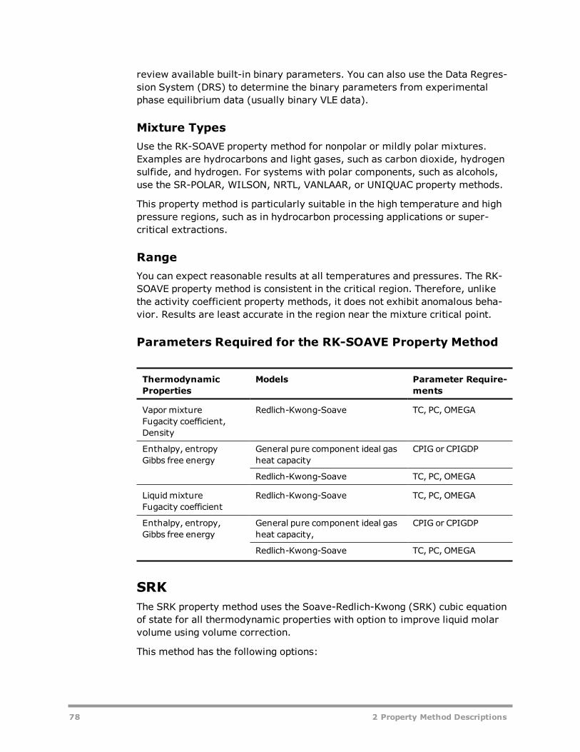
review available built-in binary parameters. You can also use the Data Regres-sion System (DRS) to determine the binary parameters from experimentalphase equilibrium data (usually binary VLE data).
Mixture TypesUse the RK-SOAVE property method for nonpolar or mildly polar mixtures.Examples are hydrocarbons and light gases, such as carbon dioxide, hydrogensulfide, and hydrogen. For systems with polar components, such as alcohols,use the SR-POLAR, WILSON, NRTL, VANLAAR, or UNIQUAC property methods.
This property method is particularly suitable in the high temperature and highpressure regions, such as in hydrocarbon processing applications or super-critical extractions.
RangeYou can expect reasonable results at all temperatures and pressures. The RK-SOAVE property method is consistent in the critical region. Therefore, unlikethe activity coefficient property methods, it does not exhibit anomalous beha-vior. Results are least accurate in the region near the mixture critical point.
Parameters Required for the RK-SOAVE Property Method
ThermodynamicProperties
Models Parameter Require-ments
Vapor mixtureFugacity coefficient,Density
Redlich-Kwong-Soave TC, PC, OMEGA
Enthalpy, entropyGibbs free energy
General pure component ideal gasheat capacity
CPIG or CPIGDP
Redlich-Kwong-Soave TC, PC, OMEGA
LiquidmixtureFugacity coefficient
Redlich-Kwong-Soave TC, PC, OMEGA
Enthalpy, entropy,Gibbs free energy
General pure component ideal gasheat capacity,
CPIG or CPIGDP
Redlich-Kwong-Soave TC, PC, OMEGA
SRKThe SRK property method uses the Soave-Redlich-Kwong (SRK) cubic equationof state for all thermodynamic properties with option to improve liquid molarvolume using volume correction.
This method has the following options:
78 2 Property Method Descriptions

l Peneloux-Rauzy method for liquid molar volume correction which resultsin more accurate liquid molar volume
l NBS Steam Table for calculating properties of water for better accuracyl Kabadi-Danner mixing rules when dealing with water-hydrocarbon sys-tems (See SRK-KD)
l Composition-independent fugacity coefficient for faster convergence inequation-based modeling
l Modified lij parameters in the SRK-ML model.
When using the SRK method, please select STEAMNBS as the free-watermethod. The NBS steam table provides greater accuracy and SRK is designed towork with it. The enthalpy, entropy, Gibbs energy, and molar volume of waterare calculated from the steam tables. The total properties are mole-fractionaverages of these values with the properties calculated by the equation of statefor other components. Fugacity coefficient is not affected.
Refer to the tables labeled Parameters Required for the SRK Property Methodbelow and Parameters Required for Common Models for thermodynamic andtransport property models, and required parameters for this property method.
This property method is comparable to other property methods based on cubicequations of state. It is recommended for gas-processing, refinery, and pet-rochemical applications. Example applications include gas plants, crude towers,and ethylene plants.
The SRK property method has built-in pure component and binary parametersfor use in modeling the ethylene process. The built-in parameters are stored inthe Ethylene databank. For other systems, you must supply pure componentand binary parameters. You can use the Data Regression System (DRS) todetermine the binary parameters from experimental phase equilibrium data(binary VLE and LLE data).
Mixture TypesUse the SRK property method for nonpolar or mildly polar mixtures. Examplesare hydrocarbons and light gases, such as carbon dioxide, hydrogen sulfide,and hydrogen. For systems with polar components, such as alcohols, use theSR-POLAR, WILSON, NRTL, VANLAAR, or UNIQUAC property methods, or spe-cify values for the lij parameters. This property method is particularly suitablein the high temperature and high pressure regions, such as in hydrocarbon pro-cessing applications or supercritical extractions.
With the Kabadi-Danner mixing rules, this property method can be used tomodel water-hydrocarbon immiscibility.
RangeYou can expect reasonable results at all temperatures and pressures. The SRKproperty method is consistent in the critical region. Therefore, unlike the activ-
2 Property Method Descriptions 79

ity coefficient property methods, it does not exhibit anomalous behavior. Res-ults are least accurate in the region near the mixture critical point.
Parameters Required for the SRK Property Method
Thermodynamic Prop-erties
Models ParameterRequirements
Vapor mixture Fugacity coef-ficient, Density
Soave-Redlich-Kwong SRKTC, SRKPC,SRKOMG
Enthalpy, entropyGibbs free energy
General pure component idealgas heat capacity
CPIG or CPIGDP
Soave-Redlich-Kwong SRKTC, SRKPC,SRKOMG
Liquidmixture Fugacity coef-ficient, Density
Soave-Redlich-Kwong SRKTC, SRKPC,SRKOMG
Enthalpy, entropy,Gibbs free energy
General pure component idealgas heat capacity
CPIG or CPIGDP
Soave-Redlich-Kwong SRKTC, SRKPC,SRKOMG
SRK-KDThe SRK-KD property method uses the SRK-Kabadi-Danner property model.This is equivalent to the SRK property method with the Kabadi-Danner mixingrules included.
The Kabadi-Danner mixing rules allow this property method to model water-hydrocarbon immiscibility. These special mixing rules handle the interactionbetween water and hydrocarbon components. The interaction is accounted forby the use of a binary interaction parameter which can be estimated fromgroup contribution.
Do not use the SRK lij parameters with the Kabadi-Danner mixing rules. Boththese methods model the asymmetric behavior of polar-hydrocarbon inter-actions, but they are not designed to be used simultaneously.
SRK-MLThe SRK-ML property method uses the SRK-ML property model. This is equi-valent to the SRK property method with an alternate set of kij parameters, andlij based on the kij.
80 2 Property Method Descriptions
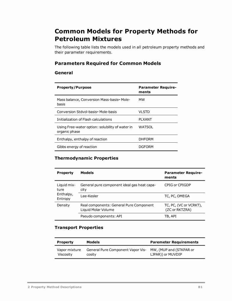
Common Models for Property Methods forPetroleum MixturesThe following table lists the models used in all petroleum property methods andtheir parameter requirements.
Parameters Required for Common Models
General
Property/Purpose Parameter Require-ments
Mass balance, Conversion Mass-basis↔Mole-basis
MW
Conversion Stdvol-basis↔Mole-basis VLSTD
Initialization of Flash calculations PLXANT
Using Free-water option: solubility of water inorganic phase
WATSOL
Enthalpy, enthalpy of reaction DHFORM
Gibbs energy of reaction DGFORM
Thermodynamic Properties
Property Models Parameter Require-ments
Liquidmix-tureEnthalpy,Entropy
General pure component ideal gas heat capa-city
CPIG or CPIGDP
Lee-Kesler TC, PC, OMEGA
Density Real components: General Pure ComponentLiquid Molar Volume
TC, PC, (VC or VCRKT),(ZC or RKTZRA)
Pseudo components: API TB, API
Transport Properties
Property Models Paremeter Requirements
Vapor mixtureViscosity
General Pure Component Vapor Vis-cosity
MW, (MUP and (STKPAR orLJPAR)) or MUVDIP
2 Property Method Descriptions 81

Property Models Paremeter Requirements
Thermal Con-ductivity
General Pure Component VaporThermal Conductivity
MW or KVDIP (and vapor vis-cosity parameters)
Diffusivity Dawson Khoury-Kobayashi MW, MUP, (STKPAR or LJPAR),VC
LiquidmixtureViscosity
API TB, API
Thermal Con-ductivity
General Pure Component LiquidThermal Conductivity
(MW, TB, TC) or KLDIP
Diffusivity Wilke-Chang MW, VB
Surface ten-sion
API TB, TC, SG
Equation-of-State PropertyMethods for High-PressureHydrocarbon ApplicationsThe following table, Equation of State Property Methods for Hydrocarbons atHigh Pressure, lists property methods for mixtures of hydrocarbons and lightgases. The property methods can deal with high pressures and temperatures,and mixtures close to their critical point (for example, pipeline transportationof gas or supercritical extraction). All thermodynamic properties of vapor andliquid phases are calculated from the equations of state. (See Equation of StateMethod in Overview of Aspen Physical Property Methods). The TRAPP modelsfor viscosity and thermal conductivity can describe the continuity of gas andliquid beyond the critical point, comparable to an equation of state.
The hydrocarbons can be from complex crude or gas mixtures treated usingpseudocomponents. But the property methods for petroleum mixtures are bet-ter tuned for these applications at low to medium pressures. Unless you use fit-ted binary interaction parameters, no great accuracy should be expected closeto the critical point. Liquid densities are not accurately predicted for the cubicequations of state.
In the presence of polar components (for example, in gas treatment), flexibleand predictive equations of state should be used. For mixtures of polar and non-polar compounds at low pressures, use an activity-coefficient-based propertymethod.
The following table lists the common and distinctive models of the propertymethods BWR-LS, LK-PLOCK, PR-BM, and RKS-BM. The parameter require-ments of the common models are given in the table labeled ParametersRequired for Common Models. The parameter requirements for the distinctive
82 2 Property Method Descriptions

models are in the tables labeled Parameters Required for the BWR-LS PropertyMethod (see BWR-LS) , Parameters Required for the BWRS Property Method(see BWRS) , Parameters Required for the LK-PLOCK Property Method (see LK-PLOCK) , Parameters Required for the PR-BM Property Method (see PR-BM) ,and Parameters Required for the RKS-BM Property Method (see RKS-BM) .
Equation-of-State Property Methods for Hydrocarbons atHigh Pressure
Property Method Name Models
BWR-LS BWR-Lee-Starling
BWRS Benedict-Webb-Rubin-Starling
LK-PLOCK Lee-Kesler-Plöcker
PR-BM Peng-Robinson-Boston-Mathias
RKS-BM Redlich-Kwong-Soave-Boston-Mathias
Property Common Models
Vapor viscosity TRAPP
Vapor thermal conductivity TRAPP
Vapor diffusivity Dawson-Khoury-Kobayashi
Surface tension API surface tension
Liquid viscosity TRAPP
Liquid thermal conductivity TRAPP
Liquid diffusivity Wilke-Chang
BWR-LSThe BWR-LS property method is based on the BWR-Lee-Starling equation ofstate. It is the generalization (in terms of pure component critical properties) ofthe Benedict-Webb-Rubin virial equation of state. The property method uses theequation of state for all thermodynamic properties. Refer to the table Para-meters Required for the BWR-LS Property Method (below) and ParametersRequired for Common Models for thermodynamic and transport property mod-els and their parameter requirements.
The BWR-LS property method is comparable to PENG-ROB, RK-SOAVE, and LK-PLOCK for phase equilibrium calculations, but is more accurate than PENG-ROBand RK-SOAVE for liquid molar volume and enthalpy. You can use it for gas
2 Property Method Descriptions 83

processing and refinery applications. It is suited for hydrogen-containing sys-tems, and has shown good results in coal liquefaction applications.
For accurate results, use the binary interaction parameters. Built-in binary para-meters BWRKV and BWRKT are available for a large number of componentpairs. The Aspen Physical Property System uses these binary parameters auto-matically. Use the Methods| Parameters | Binary Interaction | BWRKV-1 and BWRKT-1 forms to review available built-in binary parameters. You canalso use the Data Regression System (DRS) to determine the binary para-meters from experimental phase equilibrium data (usually binary VLE data).
Mixture TypesUse the BWR-LS property method for nonpolar or slightly polar mixtures, andlight gases. Asymmetric interactions between long and short molecules are wellpredicted.
RangeYou can expect reasonable results up to medium pressures. At very high pres-sures, unrealistic liquid-liquid demixing may be predicted. High pressure liquid-liquid demixing occurs between short and long chain hydrocarbons and also, forexample, between carbon dioxide and longer hydrocarbon chains at high pres-sures.
Parameters Required for the BWR-LS Property Method
Thermodynamic Prop-erties
Models Parameter Require-ments
Vapor mixtureFugacity coefficient,Density
BWR-Lee-Starling TC, VC, OMEGA
Enthalpy,Entropy,Gibbs energy
General pure component ideal gasheat capacity
CPIG or CPIGDP
BWR-Lee-Starling TC, VC, OMEGA
LiquidmixtureFugacity coefficient,Density
BWR-Lee-Starling TC, VC, OMEGA
Enthalpy,Entropy,Gibbs energy
General pure component ideal gasheat capacity
CPIG or CPIGDP
BWR-Lee-Starling TC, VC, OMEGA
84 2 Property Method Descriptions
BWRSThe BWRS property method is based on the Benedict-Webb-Rubin-Starling equa-tion of state with optional pure-component and binary interaction parameters.This equation has eleven pure-component parameters along with binary inter-action parameters. These parameters are obtained from multiproperty (vapor-liquid-equilibrium, enthalpy, PVT, etc.) data regressions. Parameters for chem-icals common to natural gas mixtures are available from Starling (1973). Ifpure-component parameters are not supplied, they are estimated with cor-relations proposed by Starling. The property method uses the equation of statefor all thermodynamic properties. Refer to the table labeled ParametersRequired for the BWRS Property Method (below) and Parameters Required forCommon Models for thermodynamic and transport property models and theirparameter requirements.
The BWRS property method is comparable to PENG-ROB, RK-SOAVE, BWR-LSand LK-PLOCK for phase equilibrium calculations, but is more accurate thanPENG-ROB and RK-SOAVE for liquid molar volume and enthalpy. You can use itfor gas processing and refinery applications. It is suited for reduced tem-peratures as low as Tr = 0.3 and reduced densities as great as ρr = 3.0. It canbe used for light hydrocarbons in the cryogenic liquid region in addition tohigher temperature regions.
For accurate results, use the binary interaction parameters. The Aspen PhysicalProperty System does not have built-in binary parameters. You can use theData Regression System (DRS) to determine the binary parameters from exper-imental phase equilibrium data (usually binary VLE data).
The BWRS method is suitable when you need very high accuracy in pure com-ponent properties. When good parameter values are given, this method can cal-culate very accurate properties (vapor pressure, molar volume, and enthalpy)for pure components. The model is also very good for light hydrocarbon sys-tems and light gases such as N2, CO2, and H2S when the binary parameters aregiven.
When water is present, by default BWRS uses the steam table to calculate theenthalpy, entropy, Gibbs energy, and molar volume of water. The total prop-erties are mole-fraction averages of these values with the properties calculatedby the equation of state for other components. Fugacity coefficient is notaffected. An option code can disable this use of the steam table.
Mixture TypesUse the BWRS property method for non-polar or slightly polar mixtures, andlight gases. Examples are hydrocarbons and light gases, such as carbon diox-ide, hydrogen sulfide, and nitrogen.
2 Property Method Descriptions 85

RangeYou can expect reasonable results at all temperatures and pressures. TheBWRS property method is consistent in the critical region. It does not exhibitanomalous behavior, unlike the activity coefficient property methods. Resultsare least accurate in the region near the mixture critical point.
Parameters Required for the BWRS Property Method
ThermodynamicProperties
Models Parameter Require-ments
Vapor mixtureFugacity coefficient,Density
Benedict-Webb-Rubin-Starling BWRSTC, BWRSVC,BWRSOM
Enthalpy,Entropy,Gibbs energy
General pure component ideal gasheat capacity
CPIG or CPIGDP
Benedict-Webb-Rubin-Starling BWRSTC, BWRSVC,BWRSOM
LiquidmixtureFugacity coefficient,Density
Benedict-Webb-Rubin-Starling BWRSTC, BWRSVC,BWRSOM
Enthalpy,Entropy,Gibbs energy
General pure component ideal gasheat capacity,
CPIG or CPIGDP
Benedict-Webb-Rubin-Starling BWRSTC, BWRSVC,BWRSOM
Reference: K. E. Starling, "Fluid Themodynamic Properties for Light PetroleumSystems", Gulf Publishing Co., Houston, Texas (1973).
LK-PLOCKThe LK-PLOCK property method is based on the Lee-Kesler-Plöcker equation ofstate, which is a virial-type equation. LK-PLOCK uses the:
l EOS to calculate all thermodynamic properties except liquid molarvolume of mixtures
l API method for liquid molar volume of pseudocomponents and the Rack-ett model for real components, in mixtures
You can use LK-PLOCK for gas-processing and refinery applications, but the RK-SOAVE or the PENG-ROB property methods are preferred.
Refer to the tables labeled Parameters Required for the LK-PLOCK PropertyMethod (below) and Parameters Required for Common Models for ther-modynamic and transport property models, and their parameter requirements.
86 2 Property Method Descriptions

For accurate results in VLE calculations, use binary parameters. Built-in binaryparameters LKPKIJ are available for a large number of component pairs. TheAspen Physical Property System uses these binary parameters automatically.Use the Methods | Parameters | Binary Interaction | LKPKIJ-1 form toreview available built-in binary parameters. You can also use the Data Regres-sion System (DRS) to determine the binary parameters from experimentalphase equilibrium data (usually binary VLE data).
This property method also has built-in correlations for estimating binary para-meters among the components CO, CO2, N2, H2, CH4, alcohols, and hydro-carbons. Components not belonging to the classes listed above are assumed tobe hydrocarbons.
Mixture TypesUse the LK-PLOCK property method for nonpolar or mildly polar mixtures.Examples are hydrocarbons and light gases, such as carbon dioxide, hydrogensulfide, and hydrogen.
RangeYou can expect reasonable results at all temperatures and pressures. The LK-PLOCK property method is consistent in the critical region. It does not exhibitanomalous behavior, unlike the activity coefficient property methods. Resultsare least accurate in the region near the mixture critical point.
Parameters Required for the LK-PLOCK Property Method
ThermodynamicProperties
Models Parameter Require-ments
Vapor mixtureFugacity coefficient,Density
Lee-Kesler-Plöcker TC, PC, VC, OMEGA
Enthalpy, entropy,Gibbs free energy
General pure component ideal gasheat capacity
CPIG or CPIGDP
Lee-Kesler-Plöcker TC, PC, VC, OMEGA
LiquidmixtureFugacity coefficient
Lee-Kesler-Plöcker TC, PC, VC, OMEGA
Density Rackett/API TB, API, TC, PC,RKTZRA
Enthalpy, entropyGibbs free energy
General pure component ideal gasheat capacity,
CPIG or CPIGDP
Lee-Kesler-Plöcker TC, PC, VC, OMEGA
2 Property Method Descriptions 87
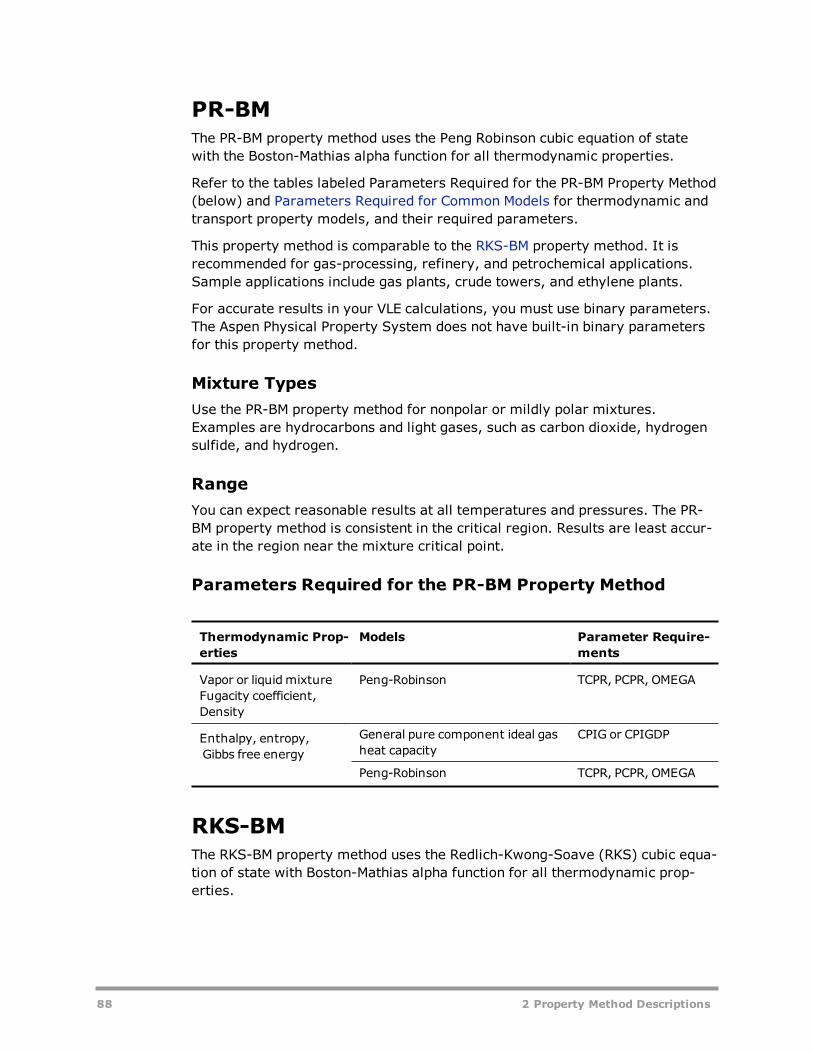
PR-BMThe PR-BM property method uses the Peng Robinson cubic equation of statewith the Boston-Mathias alpha function for all thermodynamic properties.
Refer to the tables labeled Parameters Required for the PR-BM Property Method(below) and Parameters Required for Common Models for thermodynamic andtransport property models, and their required parameters.
This property method is comparable to the RKS-BM property method. It isrecommended for gas-processing, refinery, and petrochemical applications.Sample applications include gas plants, crude towers, and ethylene plants.
For accurate results in your VLE calculations, you must use binary parameters.The Aspen Physical Property System does not have built-in binary parametersfor this property method.
Mixture TypesUse the PR-BM property method for nonpolar or mildly polar mixtures.Examples are hydrocarbons and light gases, such as carbon dioxide, hydrogensulfide, and hydrogen.
RangeYou can expect reasonable results at all temperatures and pressures. The PR-BM property method is consistent in the critical region. Results are least accur-ate in the region near the mixture critical point.
Parameters Required for the PR-BM Property Method
Thermodynamic Prop-erties
Models Parameter Require-ments
Vapor or liquidmixtureFugacity coefficient,Density
Peng-Robinson TCPR, PCPR, OMEGA
Enthalpy, entropy,Gibbs free energy
General pure component ideal gasheat capacity
CPIG or CPIGDP
Peng-Robinson TCPR, PCPR, OMEGA
RKS-BMThe RKS-BM property method uses the Redlich-Kwong-Soave (RKS) cubic equa-tion of state with Boston-Mathias alpha function for all thermodynamic prop-erties.
88 2 Property Method Descriptions

This property method is comparable to the PR-BM property method. It is recom-mended for gas-processing, refinery, and petrochemical applications. Exampleapplications include gas plants, crude towers, and ethylene plants.
For accurate results in your VLE calculations, you must use binary parameters.The binary parameters available are automatically retrieved from the EOS-LITdatabank.
Mixture TypesUse the RKS-BM property method for nonpolar or mildly polar mixtures.Examples are hydrocarbons and light gases, such as carbon dioxide, hydrogensulfide, and hydrogen.
RangeYou can expect reasonable results at all temperatures and pressures. The RKS-BM property method is consistent in the critical region. Results are least accur-ate in the region near the mixture critical point.
Refer to the tables labeled Parameters Required for the RKS-BM PropertyMethod (below) and Parameters Required for Common Models for ther-modynamic and transport property models, and their required parameters.
Parameters Required for the RKS-BM Property Method
Thermodynamic Prop-erties
Models Parameter Require-ments
Vapor or liquidmixtureFugacity coefficient,Density
Redlich-Kwong-Soave TCRKS, PCRKS,OMGRKS
Enthalpy, entropy,Gibbs free energy
General pure component ideal gasheat capacity
CPIG or CPIGDP
Redlich-Kwong-Soave TCRKS, PCRKS,OMGRKS
Common Models for Equation-of-State Prop-erty Methods for High-Pressure Hydro-carbon ApplicationsThe following table lists the models common to equation-of-state propertymethods for high–pressure hydrocarbon applications and their parameterrequirements.
2 Property Method Descriptions 89

Parameters Required for Common Models
General
Property/Purpose Parameter Require-ments
Mass balance,Conversion Mass-basis↔Mole-basis
MW
Conversion Stdvol-basis↔Mole-basis VLSTD
Initialization of Flash calculations PLXANT
Using Free-water option: solubility of water inorganic phase
WATSOL
Enthalpy, enthalpy of reaction DHFORM
Gibbs energy of reaction DGFORM
Transport
Property Models Parameter Requirements
Vapor MixtureViscosity
TRAPP TC, PC, OMEGA
Thermal Conductivity TRAPP TC, PC, OMEGA
Diffusivity Dawson-Khoury-Kobay-ashi
MW, MUP, (STKPAR or LJPAR), VC
Surface tension API TB, TC, SG
LiquidmixtureViscosity
TRAPP TC, PC, OMEGA
Thermal Conductivity TRAPP TC, PC, OMEGA
Diffusivity Wilke-Chang MW, VB
Flexible and Predictive Equa-tion-of-State Property MethodsThe table labeled Flexible and Predictive Equation-of-State Property Methods(below) lists property methods for mixtures of polar and non-polar componentsand light gases. The property methods can deal with high pressures and tem-peratures, mixtures close to their critical point, and liquid-liquid separation at
90 2 Property Method Descriptions

high pressure. Examples of applications are gas drying with glycols, gas sweet-ening with methanol, and supercritical extraction.
Pure component thermodynamic behavior is modeled using the Peng-Robinsonor Redlich-Kwong-Soave equations of state. They are extended with flexiblealpha-functions with up to three parameters, for very accurate fitting of vaporpressures. This is important in separations of very closely boiling systems andfor polar compounds. In some cases they are extended with a volume trans-lation term for accurate fitting of liquid densities (see the table labeled Flexibleand Predictive Equation-of-State Property Methods below).
Parameters for the Schwartzentruber-Renon and Mathias-Copeman alpha func-tions are available for many components in the PURECOMP databank.
Mixing rules for these models vary. Extended classical mixing rules are usedfor fitting hydrogen-rich systems or systems with strong size and shape asym-metry (Redlich-Kwong-Aspen). Composition and temperature-dependent mix-ing rules fit strongly non-ideal high pressure systems (SR-POLAR). ModifiedHuron-Vidal mixing rules can predict non-ideality at high pressure from low-pressure (group-contribution) activity coefficient models (Wong-Sandler,MHV2, PSRK). The predictive capabilities of modified Huron-Vidal mixing rulesare superior to the predictive capabilities of SR-POLAR. The differences amongcapabilities of the modified Huron-Vidal mixing rules are small (see PhysicalProperty Models).
The Wong-Sandler, MHV2, and Holderbaum-Gmehling mixing rules use activitycoefficient models to calculate excess Gibbs or Helmholtz energy for the mixingrules. The property methods with these mixing rules use the UNIFAC or Lyngbymodified UNIFAC group contribution models. Therefore, they are predictive.You can use any Aspen Physical Property System activity coefficient modelswith these mixing rules, including user models. Use the Properties MethodsModels sheet to modify the property method. See Modifying and Creating Prop-erty Methods for details on how to modify a property method.
The Chung-Lee-Starling models for viscosity and thermal conductivity candescribe the continuity of gas and liquid beyond the critical point. This is com-parable to an equation of state. These models can fit the behavior of polar andassociating components. Details about the pure component models and mixingrules are found in Physical Property Models.
For mixtures of polar and non-polar compounds at low pressures, activity coef-ficient models are preferred. For non-polar mixtures of petroleum fluids andlight gases at low to medium pressures, the property methods for petroleummixtures are recommended. The flexible and predictive equations of state arenot suited for electrolyte solutions.
The following table, Flexible and Predictive Equation-of-State Property Meth-ods, lists flexible and predictive equation-of-state property methods, the dis-tinctive equation-of-state models on which they are based, and some of theircharacteristics. The table also gives the models that the property methods havein common. Parameter requirements of the common models are given in the
2 Property Method Descriptions 91

table labeled Parameters Required for Common Flexible and Predictive Models.Parameter requirements for the distinctive models are in the tables labeledParameters Required for the PRMHV2 Property Method (see PRMHV2), Para-meters Required for the PRWS Property Method (see PRWS), ParametersRequired for the PSRK Property Method (see PSRK), Parameters Required forthe RK-ASPEN Property Method (RK-ASPEN), Parameters Required for theRKSMHV2 Property Method (see RKSMHV2), Parameters Required for theRKSWS Property Method (see RKSWS), and Parameters Required for the SR-POLAR Property Method (see SR-POLAR).
Flexible and Predictive Equation-of-State Property Methods
PropertyMethod Name
Equation ofState
VolumeShift
Mixing Rule Predictive
HYSGLYCO Twu-Sim-Tassone — — X
PC-SAFT Copolymer PC-SAFT
— — —
PRMHV2 Peng-Robinson — MHV2 X
PRWS Peng-Robinson — Wong-Sandler X
PSRK Redlich-Kwong-Soave
— Holderbaum-Gmehling
X
RK-ASPEN Redlich-Kwong-Soave
— Mathias —
RKSMHV2 Redlich-Kwong-Soave
— MHV2 X
RKSWS Redlich-Kwong-Soave
— Wong-Sandler X
SR-POLAR Redlich-Kwong-Soave
X Schwarzentruber-Renon
—
An X in the Volume Shift column indicates volume shift is included in the prop-erty method.
An X in the Predictive column indicates that the property method is predictive.
Property Common Models
Vapor viscosity Chung-Lee-Starling
Vapor thermal con-ductivity
Chung-Lee-Starling
Vapor diffusivity Dawson-Khoury-Kobayashi
92 2 Property Method Descriptions

Property Common Models
Surface tension General Pure Component Liquid SurfaceTension
Liquid viscosity Chung-Lee-Starling
Thermal conductivity Chung-Lee-Starling
Liquid diffusivity Wilke-Chang liquid
CPAThe CPA method represents the Cubic-Plus-Association EOS model developedby Kontogeorgis and co-workers (Kontogeorgis, Voutsas, Yakoumis, Tassios,IECR 1996). The model combines the SRK cubic EOS with an association termsimilar to that of SAFT, as present in the PC-SAFT model. Mixing rules apply tothe cubic, whereas combining rules are used for the association term. Themodel’s applicability covers the VLE and VLLE of mixtures containing hydro-carbons and polar/associating chemicals such as water, alcohols, glycols,esters, and organic acids.
The CPA (Cubic-Plus-Association) property method uses the Soave-Redlich-Kwong (SRK) cubic equation of state combined with the association term forSAFT for all thermodynamic properties.
Refer to the tables labeled Parameters Required for the CPA Property Methodbelow and Parameters Required for Common Models for thermodynamic andtransport property models, and required parameters for this property method.
In the absence of associating (hydrogen-bonding) species, this propertymethod reduces to the SRK model, widely used for gas-processing, refinery,petrochemical applications. The addition of the association term for com-ponents capable of exhibiting hydrogen-bonding (water, alcohols, glycols,acids) enables CPA to better model the V(L)LE of complex systems.
The CPA property method has built-in pure component and binary parametersfor use in modeling processes such as Methanol gas cleaning. The built-in para-meters are stored in the AP-EOS databank. For species not in the databank,Aspen Properties will estimate the non-associating pure component parametersfrom the critical temperature, critical pressure, and acentric factor. We recom-mend however, and necessary for associating components, that you use theData Regression System (DRS) to determine the pure component parametersfrom vapor pressure and liquid density data, and the binary parameters fromexperimental phase equilibrium data (binary VLE and LLE data).
Mixture TypesUse the CPA property method for nonpolar or associating mixtures. Examplesare hydrocarbons and light gases, such as carbon dioxide, hydrogen sulfide,and hydrogen. For systems with associating (polar) components, such as
2 Property Method Descriptions 93
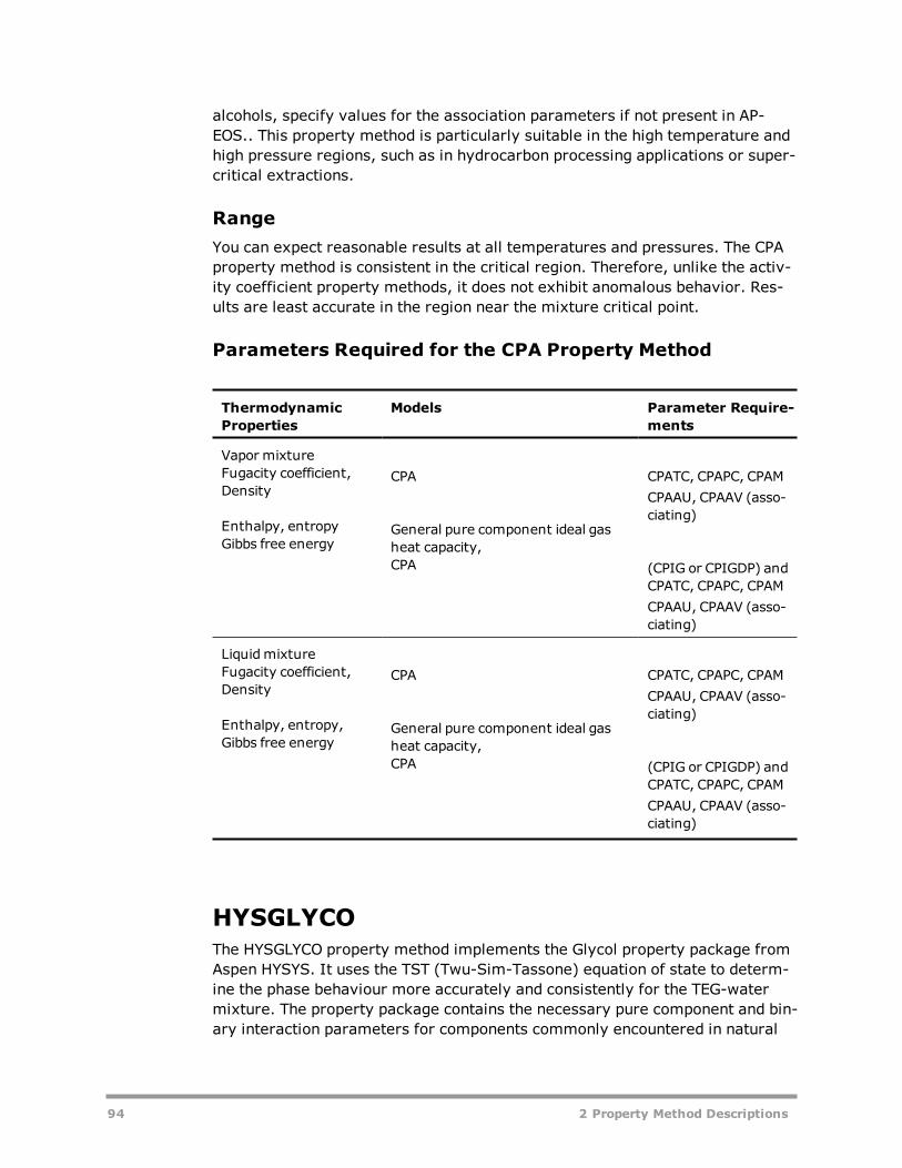
alcohols, specify values for the association parameters if not present in AP-EOS.. This property method is particularly suitable in the high temperature andhigh pressure regions, such as in hydrocarbon processing applications or super-critical extractions.
RangeYou can expect reasonable results at all temperatures and pressures. The CPAproperty method is consistent in the critical region. Therefore, unlike the activ-ity coefficient property methods, it does not exhibit anomalous behavior. Res-ults are least accurate in the region near the mixture critical point.
Parameters Required for the CPA Property Method
ThermodynamicProperties
Models Parameter Require-ments
Vapor mixtureFugacity coefficient,Density
Enthalpy, entropyGibbs free energy
CPA
General pure component ideal gasheat capacity,CPA
CPATC, CPAPC, CPAMCPAAU, CPAAV (asso-ciating)
(CPIG or CPIGDP) andCPATC, CPAPC, CPAMCPAAU, CPAAV (asso-ciating)
LiquidmixtureFugacity coefficient,Density
Enthalpy, entropy,Gibbs free energy
CPA
General pure component ideal gasheat capacity,CPA
CPATC, CPAPC, CPAMCPAAU, CPAAV (asso-ciating)
(CPIG or CPIGDP) andCPATC, CPAPC, CPAMCPAAU, CPAAV (asso-ciating)
HYSGLYCOThe HYSGLYCO property method implements the Glycol property package fromAspen HYSYS. It uses the TST (Twu-Sim-Tassone) equation of state to determ-ine the phase behaviour more accurately and consistently for the TEG-watermixture. The property package contains the necessary pure component and bin-ary interaction parameters for components commonly encountered in natural
94 2 Property Method Descriptions

gas dehydration process. The property package is tuned to represent accur-ately, the phase behaviour of these components, especially that for the TEG-water binary system.
The TST equation of state can accurately predict:
l activity coefficients of the TEG-water solutions within the average abso-lute deviation of 2%
l dew point temperatures within an average error of ±1°C.l water content of gas within the average absolute deviation of 1%
The Glycol property package should be applicable over the range of tem-peratures, pressures, and component concentration encountered in a typicalTEG-water dehydration system: between 15°C to 50°C and between 10 atm to100 atm for the gas dehydrator, and between 202°C to 206°C and 1.2 atmo-spheres for the glycol regenerator.
The accuracy of predicted solubility of hydrocarbons in aqueous phase is expec-ted to be within the experimental uncertainty.
The table below displays the prediction of equilibrium water content inlbH2O/MMSCF for a gas stream in contact with 99.5 weight percent TEG, usingthe Glycol property package.
T dew (K) Reported by: Predicted from TST (EOS):
McKetta Bukacek Water Con-tent
Pressure(Pa)
277.59 390 396 393 838
266.48 170 176 174 370
255.37 70 72 71 151
244.26 28 27 26 56.1
233.15 9.2 9.1 9 18.7
222.04 2.4 2.8 2.6 6
The BIP databank for the Glycol property package is continuously updated. Cur-rently, there may be some limitations or missing BIP for certain componentpairs. For example, heavy hydrocarbons or hypothetical components whichmay not have any interaction parameters available.
Glycol Calculation MethodsFor the Glycol property package, three alpha function parameters are used tocorrelate the vapor pressure of the component in the HYSYS componentdatabank. The alpha function parameters are: L, M, and N parameters that areunique for each component.
2 Property Method Descriptions 95

For Glycol property package, three adjustable parameters are used to correlateVapor-Liquid-Equilibrium (VLE) mixture data. The parameters corresponding tothe TST (Twu-Sim-Tassone) AE mixing rules are Aij, Aji, and αij binary inter-action parameters in the NRTL equation. The Glycol property package uses theCavett model for enthalpy and entropy calculations.
Parameters used by the HYSGLYCO property method:
l GLYABV: Glycol EOS activity binary parameters Aij, Bij and Cijl GLYKIJ: Glycol EOS binary parameterl GLYLMN: Parameters for the Twu Alpha functionl PCGLY: Critical pressurel TCGLY: Critical temperature
These parameters and others used by HYSGLYCO are available in the HYSYSdatabank. When using HYSGLYCO it is recommended to place the HYSYSdatabank in the search order before other databanks.
The liquid thermal conductivity model uses API methods rather than the HYSYSmodel for pseudocomponents:
l API equation 12A3.2-1 for normal boiling point Tb above 337 Kl API equation 12A1.2-1 for other components with molecular weightabove 140 and reduced temperature Tr=T/Tc below 0.8
With option code 1 set to 1 in KL2GLY and KL0GLY, API equation 12A1.2-1 isused for all components.
Option code 1 of ESGLY and ESGLY0 controls the volume root search method.The default is 0, to use an analytical solution. This analytical solution may pro-duce a wrong root in some cases, such as with some pure water streams. If youget results showing the wrong phase with HYSGLYCO and such streams, changethis option code to 1 to use the numerical solution. See Option Codes for Equa-tion of State Models in Physical Property Models for information about otheroption codes.
For more information on the Glycol package, see Aspen HYSYS help.
PC-SAFT: Copolymer PC-SAFT EOS PropertyMethodThe PC-SAFT method represents the copolymer PC-SAFT EOS model developedby Sadowski and co-workers (Gross and Sadowski, 2001, 2002a, 2002b; Grosset al., 2003; Becker et al., 2004; Kleiner et al., 2006). Unlike the POLYPCSFmethod, the copolymer PC-SAFT includes the association and polar terms anddoes not apply mixing rules to calculate the copolymer parameters from its seg-ments. Its applicability covers fluid systems from small to large molecules,including normal fluids, water, alcohols, and ketones, polymers and copoly-mers and their mixtures.
96 2 Property Method Descriptions
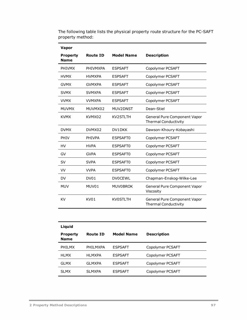
The following table lists the physical property route structure for the PC-SAFTproperty method:
Vapor
PropertyName
Route ID Model Name Description
PHIVMX PHIVMXPA ESPSAFT Copolymer PCSAFT
HVMX HVMXPA ESPSAFT Copolymer PCSAFT
GVMX GVMXPA ESPSAFT Copolymer PCSAFT
SVMX SVMXPA ESPSAFT Copolymer PCSAFT
VVMX VVMXPA ESPSAFT Copolymer PCSAFT
MUVMX MUVMX02 MUV2DNST Dean-Stiel
KVMX KVMX02 KV2STLTH General Pure Component VaporThermal Conductivity
DVMX DVMX02 DV1DKK Dawson-Khoury-Kobayashi
PHIV PHIVPA ESPSAFT0 Copolymer PCSAFT
HV HVPA ESPSAFT0 Copolymer PCSAFT
GV GVPA ESPSAFT0 Copolymer PCSAFT
SV SVPA ESPSAFT0 Copolymer PCSAFT
VV VVPA ESPSAFT0 Copolymer PCSAFT
DV DV01 DV0CEWL Chapman-Enskog-Wilke-Lee
MUV MUV01 MUV0BROK General Pure Component VaporViscosity
KV KV01 KV0STLTH General Pure Component VaporThermal Conductivity
Liquid
PropertyName
Route ID Model Name Description
PHILMX PHILMXPA ESPSAFT Copolymer PCSAFT
HLMX HLMXPA ESPSAFT Copolymer PCSAFT
GLMX GLMXPA ESPSAFT Copolymer PCSAFT
SLMX SLMXPA ESPSAFT Copolymer PCSAFT
2 Property Method Descriptions 97

Liquid
PropertyName
Route ID Model Name Description
VLMX VLMXPA ESPSAFT Copolymer PCSAFT
MULMX MULMX13 MUPOLY,MULMH
Aspen, Modified Mark-Houwink/van Krevelen, Andrade
KLMX KLMXVKTR KLMXVKTR Vredeveldmixing, Modified vanKrevelen, TRAPP
DLMX DLMX02 DL1WCA Wilke-Chang-Andrade
SIGLMX SIGLMX01 SIG2HSS General Pure Component LiquidSurface Tension, Power Law Mix-ing
PHIL PHILPA ESPSAFT0 Copolymer PCSAFT
HL HLPA ESPSAFT0 Copolymer PCSAFT
GL GLPA ESPSAFT0 Copolymer PCSAFT
SL SLPA ESPSAFT0 Copolymer PCSAFT
VL VLPA ESPSAFT0 Copolymer PCSAFT
DL DL01 DL0WCA Wilke-Chang-Andrade
MUL MULMH MUL0MH Modified Mark-Houwink/vanKrevelen, Andrade
KL KL0VKTR KL0VKTR Modified van Krevelen, TRAPP
Solid
PropertyName
Route ID Model Name Description
HSMX HSMXDVK HS0DVK Ideal mixing, van Krevelen
GSMX GSMXDVK GS0DVK Ideal mixing, van Krevelen
SSMX SSMXDVK HS0DVK,GS0DVK
Ideal mixing, van Krevelen
VSMX VSMXDVK VS0DVK,VS0POLY
van Krevelen, Polynomial
HS HSDVK HS0DVK van Krevelen
GS GSDVK GS0DVK van Krevelen
98 2 Property Method Descriptions
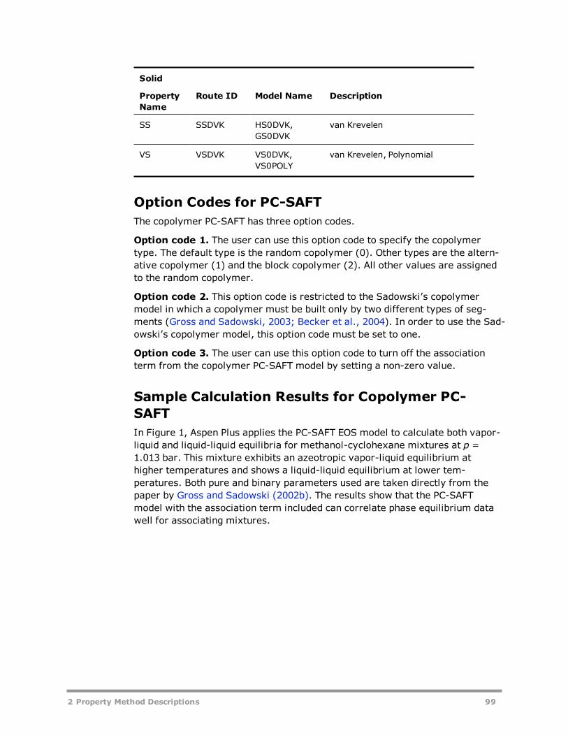
Solid
PropertyName
Route ID Model Name Description
SS SSDVK HS0DVK,GS0DVK
van Krevelen
VS VSDVK VS0DVK,VS0POLY
van Krevelen, Polynomial
Option Codes for PC-SAFTThe copolymer PC-SAFT has three option codes.
Option code 1. The user can use this option code to specify the copolymertype. The default type is the random copolymer (0). Other types are the altern-ative copolymer (1) and the block copolymer (2). All other values are assignedto the random copolymer.
Option code 2. This option code is restricted to the Sadowski’s copolymermodel in which a copolymer must be built only by two different types of seg-ments (Gross and Sadowski, 2003; Becker et al., 2004). In order to use the Sad-owski’s copolymer model, this option code must be set to one.
Option code 3. The user can use this option code to turn off the associationterm from the copolymer PC-SAFT model by setting a non-zero value.
Sample Calculation Results for Copolymer PC-SAFTIn Figure 1, Aspen Plus applies the PC-SAFT EOS model to calculate both vapor-liquid and liquid-liquid equilibria for methanol-cyclohexane mixtures at p =1.013 bar. This mixture exhibits an azeotropic vapor-liquid equilibrium athigher temperatures and shows a liquid-liquid equilibrium at lower tem-peratures. Both pure and binary parameters used are taken directly from thepaper by Gross and Sadowski (2002b). The results show that the PC-SAFTmodel with the association term included can correlate phase equilibrium datawell for associating mixtures.
2 Property Method Descriptions 99

Figure 1. Isobaric vapor-liquid and liquid-liquid equilibria of methanol-cyc-lohexane at = 1.013 bar. Experimental data are taken from Jones andAmstell (1930) and Marinichev and Susarev (1965).
Figure 2 shows a model calculation for HDPE-Hexane mixtures. This systemexhibits both lower critical solution temperature (LCST) and upper critical solu-tion temperature (UCST) at p = 50 bar. The pure parameters are taken directlyfrom papers Gross and Sadowski (2001; 2002a). The binary parameterbetween hexane and ethylene segment is set to 0.012. The phase equilibriumcalculations are carried by Flash3 block with Gibbs flash algorithm in AspenPlus.
100 2 Property Method Descriptions
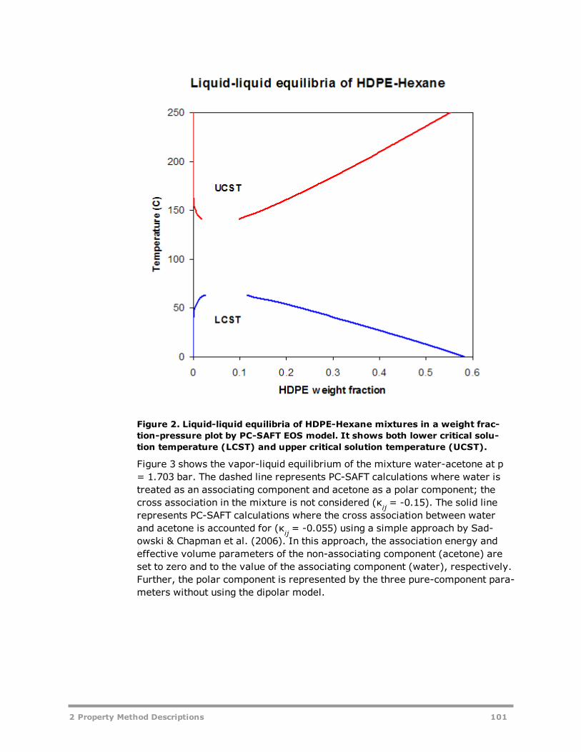
Figure 2. Liquid-liquid equilibria of HDPE-Hexane mixtures in a weight frac-tion-pressure plot by PC-SAFT EOS model. It shows both lower critical solu-tion temperature (LCST) and upper critical solution temperature (UCST).
Figure 3 shows the vapor-liquid equilibrium of the mixture water-acetone at p= 1.703 bar. The dashed line represents PC-SAFT calculations where water istreated as an associating component and acetone as a polar component; thecross association in the mixture is not considered (κij = -0.15). The solid linerepresents PC-SAFT calculations where the cross association between waterand acetone is accounted for (κij = -0.055) using a simple approach by Sad-owski & Chapman et al. (2006). In this approach, the association energy andeffective volume parameters of the non-associating component (acetone) areset to zero and to the value of the associating component (water), respectively.Further, the polar component is represented by the three pure-component para-meters without using the dipolar model.
2 Property Method Descriptions 101
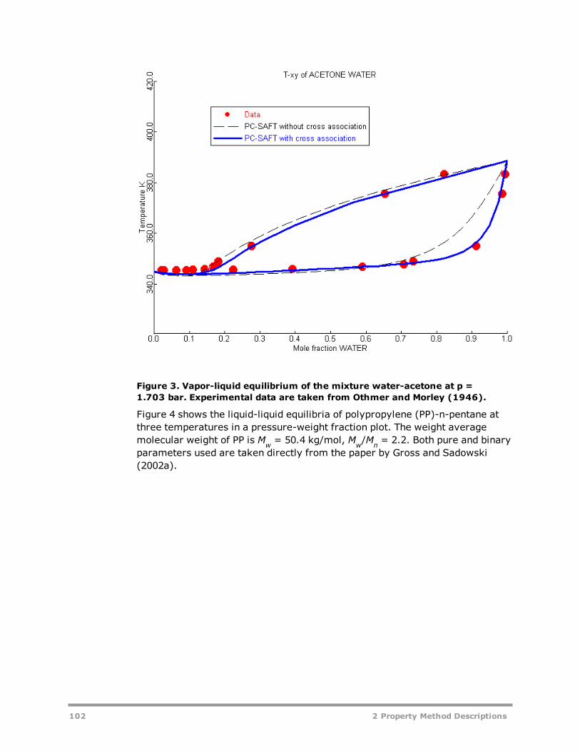
Figure 3. Vapor-liquid equilibrium of the mixture water-acetone at p =1.703 bar. Experimental data are taken from Othmer and Morley (1946).
Figure 4 shows the liquid-liquid equilibria of polypropylene (PP)-n-pentane atthree temperatures in a pressure-weight fraction plot. The weight averagemolecular weight of PP is Mw = 50.4 kg/mol, Mw/Mn = 2.2. Both pure and binaryparameters used are taken directly from the paper by Gross and Sadowski(2002a).
102 2 Property Method Descriptions

Figure 4. Liquid-liquid equilibria of PP-n-Pentane at three different tem-peratures. Comparison of experimental cloud points (Martin et al., 1999) toPC-SAFT calculations (κij = 0.0137). The polymer was assumed to be mon-odisperse at Mw = 50.4 kg/mol.
ReferencesBecker, F., Buback, M., Latz, H., Sadowski, G., & Tumakaka, F. (2004). Cloud-Point Curves of Ethylene-(Meth)acrylate Copolymers in Fluid Ethene up to HighPressures and Temperatures – Experimental Study and PC-SAFT Modeling.Fluid Phase Equilibria, 215, 263-282.
Gross, J., & Sadowski, G. (2001). Perturbed-Chain SAFT: An Equation of StateBased on a Perturbation Theory for Chain Molecules. Ind. Eng. Chem. Res., 40,1244-1260.
Gross, J., & Sadowski, G. (2002a). Modeling Polymer Systems Using the Per-turbed-Chain Statistical Associating Fluid Theory Equation of State. Ind. Eng.Chem. Res., 41, 1084-1093.
Gross, J., & Sadowski, G. (2002b). Application of the Perturbed-Chain SAFTEquation of State to Associating Systems. Ind. Eng. Chem. Res., 41, 5510-5515.
2 Property Method Descriptions 103

Gross, J., Spuhl, O., Tumakaka, F., & Sadowski, G. (2003). Modeling Copoly-mer Systems Using the Perturbed-Chain SAFT Equation of State. Ind. Eng.Chem. Res., 42, 1266-1274.
Jones, D. C., & Amstell, S. (1930). J. Chem. Soc., 1316.
Kleiner, M., Tumakaka, F., Sadowski, G., Dominik, A., Jain, S., Bymaster, A., &Chapman, W. G. (2006). Thermodynamic Modeling of Complex Fluids using PC-SAFT. Final Report for Consortium of Complex Fluids. Universität Dortmund &Rice University.
Marinichev, A.N., & Susarev, M.P. (1965). Zh. Prikl. Khim., 38, 1619.
Martin, T. M., Lateef, A. A., & Roberts, C. B. (1999). Measurements and mod-eling of cloud point behavior for polypropylene/n-pentane and polypropylene/n-pentane/carbon dioxide mixtures at high pressures. Fluid Phase Equilibria, 154,241.
Othmer, D. F., & Morley, F. R. (1946). Composition of Vapors from Boiling Bin-ary Solutions – Apparatus for Determinations under Pressure. Ind. Eng. Chem.,38, 751-757.
PRMHV2The PRMHV2 property method is based on the Peng-Robinson-MHV2 equation-of-state model, which is an extension of the Peng-Robinson equation of state.The UNIFAC model is used by default to calculate excess Gibbs energy in theMHV2 mixing rules. Other modified UNIFAC models and activity coefficient mod-els can be used for excess Gibbs energy.
Besides the acentric factor, up to three polar parameters can be used to fitmore accurately the vapor pressure of polar compounds.
The MHV2 mixing rules predict the binary interactions at any pressure. Usingthe UNIFAC model the MHV2 mixing rules are predictive for any interaction thatcan be predicted by the UNIFAC model at low pressure.
The minimum parameter requirements of the PRMHV2 property method aregiven in the tables labeled Parameters Required for the PRMHV2 PropertyMethod (below) and Parameters Required for Common Flexible and PredictiveModels. For details about optional parameters, and calculation of pure com-ponent and mixture properties, see Physical Property Models.
Mixture TypesYou can use the PRMHV2 property method for mixtures of non-polar and polarcompounds. For light gases UNIFAC does not provide any interaction.
RangeYou can use the PRMHV2 property method up to high temperatures and pres-sures. You can expect accurate predictions (4% in pressure and 2% in mole
104 2 Property Method Descriptions
fraction at given temperature) up to about 150 bar. You can expect reasonableresults at any condition, provided the UNIFAC interaction parameters are avail-able. Results are least accurate close to the critical point.
Parameters Required for the PRMHV2 Property Method
ThermodynamicProperties
Models Parameter Require-ments
Vapor and liquidmixtureFugacity coefficient,Density
Peng-Robinson-MHV2, TC, PC, OMEGA
UNIFAC UFGRP, GMUFQ,GMUFR
Enthalpy,Entropy,Gibbs energy
General pure component ideal gasheat capacity
CPIG or CPIGDP
Peng-Robinson-MHV2 TC, PC, OMEGA
UNIFAC UFGRP, GMUFQ,GMUFR
PRWSThe PRWS property method is based on the Peng-Robinson-Wong-Sandler equa-tion-of-state model, which is based on an extension of the Peng-Robinson equa-tion of state. The UNIFAC model is used to calculate excess Helmholtz energyfor the mixing rules.
Besides the acentric factor, you can use up to three polar parameters to fitmore accurately the vapor pressure of polar compounds. The Wong-Sandlermixing rules predict the binary interactions at any pressure. Using the UNIFACmodel the PRWS property method is predictive for any interaction that can bepredicted by UNIFAC at low pressure.
The minimum parameter requirements of the property method are given in thetables labeled Parameters Required for the PRWS Property Method (below) andParameters Required for Common Flexible and Predictive Models. For detailsabout the optional parameters, and about calculation of pure component andmixture properties, see Physical Property Models.
Mixture TypesYou can use the PRWS property method for mixtures of non-polar and polarcompounds, in combination with light gases.
RangeYou can use the PRWS property method up to high temperatures and pressures.You can expect accurate predictions (3% in pressure and 2% in mole fraction ata given temperature) up to about 150 bar. You can expect reasonable results at
2 Property Method Descriptions 105

any condition, provided UNIFAC interaction parameters are available. Resultsare least accurate close to the critical point.
Parameters Required for the PRWS Property Method
Thermodynamic Prop-erties
Models Parameter Require-ments
Vapor and liquidmixtureFugacity coefficient,Density
Peng-Robinson-WS TC, PC, OMEGA
UNIFAC UFGRP, GMUFR,GMUFQ
Enthalpy,Entropy,Gibbs energy
General pure component ideal gasheat capacity
CPIG or CPIGDP)
Peng-Robinson-WS TC, PC, OMEGA
UNIFAC UFGRP, GMUFR,GMUFQ
PSRKThe PSRK property method is based on the Predictive Soave-Redlich-Kwongequation-of-state model, which is an extension of the Redlich-Kwong-Soaveequation of state.
Besides the acentric factor, you can use up to three polar parameters to fitmore accurately the vapor pressure of polar compounds. The Holderbaum-Gmehling mixing rules or PSRK method predict the binary interactions at anypressure. Using UNIFAC the PSRK method is predictive for any interaction thatcan be predicted by UNIFAC at low pressure. The UNIFAC interaction para-meter table has been extended for gases, for the PSRK method.
The minimum parameter requirements of the PSRK property method are givenin the tables labeled Parameters Required for the PSRK Property Method (seebelow) and Parameters Required for Flexible and Predictive Models. For detailsabout the optional parameters, and about calculation of pure component andmixture properties, see Physical Property Models.
Mixture TypesYou can use the PSRK property method for mixtures of non-polar and polar com-pounds, in combination with light gases.
RangeYou can use the PSRK property method up to high temperatures and pressures.You can expect accurate predictions at any conditions provided UNIFAC inter-
106 2 Property Method Descriptions

action parameters are available. Results are least accurate close to the criticalpoint.
Parameters Required for the PSRK Property Method
ThermodynamicProperties
Models Parameter Require-ments
Vapor and liquidmixtureFugacity coef-ficient, Density
PSRK TC, PC, OMEGA
UNIFAC UFGRP, GMUFR, GMUFQ
Enthalpy,Entropy,Gibbs energy
General pure component ideal gasheat capacity
CPIG or CPIGDP
PSRK TC, PC, OMEGA,
UNIFAC UFGRP, GMUFR, GMUFQ
RK-ASPENThe RK-ASPEN property method is based on the Redlich-Kwong-Aspen equa-tion-of-state model, which is an extension of Redlich-Kwong-Soave.
This property method is similar to RKS-BM, but it also applies to polar com-ponents such as alcohols and water. RK-ASPEN requires polar parameters thatmust be determined from regression of experimental vapor pressure data usingDRS. Use the binary parameters to obtain best possible results for phase equi-libria. RK-ASPEN allows temperature-dependent binary parameters. If thepolar parameters are zero for all components and the binary parameters areconstant, RK-ASPEN is identical to RKS-BM.
The minimum parameter requirements of the RK-ASPEN property method aregiven in the tables labeled Parameters Required for the RK-ASPEN PropertyMethod (see below) and Parameters Required for Common Flexible and Pre-dictive Models. For details about the optional parameters for this model, seePhysical Property Models.
Mixture TypesYou can use the RK-ASPEN property method for mixtures of non-polar andslightly polar compounds, in combination with light gases. It is especially suitedfor combinations of small and large molecules, such as nitrogen with n-Decane,or hydrogen-rich systems.
2 Property Method Descriptions 107
RangeYou can use the RK-ASPEN property method up to high temperatures and pres-sures. You can expect reasonable results at any condition, but results are leastaccurate close to the critical point.
Parameters Required for the RK-ASPEN Property Method
ThermodynamicProperties
Models Parameter Requirements
Vapor and liquidmix-tureFugacity coefficient,Density
Redlich-Kwong-Aspen TCRKA, PCRKA, OMEGARKAUFGRP, GMUFR, GMUFQ
Enthalpy,Entropy,Gibbs energy
General pure componentideal gas heat capacity
CPIG or CPIGDP
Redlich-Kwong-Aspen TCRKA, PCRKA, OMEGARKA
RKSMHV2The RKSMHV2 property method is based on the Redlich-Kwong-Soave MHV2equation-of-state model, which is an extension of the Redlich-Kwong-Soaveequation of state. The Lyngby modified UNIFAC model is used to calculateexcess Gibbs energy for the MHV2 mixing rules.
Besides the acentric factor, you can use up to three polar parameters to fitmore accurately the vapor pressure of polar compounds. The MHV2 mixingrules predict the binary interactions at any pressure. Using the Lyngby modifiedUNIFAC model, the Redlich-Kwong-Soave MHV2 model is predictive for anyinteraction that can be predicted by Lyngby modified UNIFAC at low pressure.The Lyngby modified UNIFAC interaction parameter table has been extendedfor gases for the MHV2 method.
The minimum parameter requirements of the RKSMHV2 property method aregiven in the tables labeled Parameters Required for the RKSMHV2 PropertyMethod (see below) and Parameters Required for Common Flexible and Pre-dictive Models. For details about optional parameters and calculation of purecomponent and mixture properties, see Physical Property Models.
Mixture TypesYou can use the RKSMHV2 property method for mixtures of non-polar and polarcompounds, in combination with light gases.
108 2 Property Method Descriptions

RangeYou can use the RKSMHV2 property method up to high temperatures and pres-sures. You can expect accurate predictions (4% in pressure and 2% in molefraction at given temperature) up to about 150 bar. You can expect reasonableresults at any condition, provided Lyngby modified UNIFAC interactions areavailable. Results are least accurate close to the critical point.
Parameters Required for the RKSMHV2 Property Method
Thermodynamic Prop-erties
Models Parameter Require-ments
Vapor and liquidmixtureFugacity coefficient,Density
Redlich-Kwong-Soave-MHV2 TC, PC, OMEGA
Lyngby modified UNIFAC UFGRPL, GMUFLR,GMUFLQ
Enthalpy,Entropy,Gibbs energy
General pure component ideal gasheat capacity
CPIG or CPIGDP
Redlich-Kwong-Soave-MHV2 TC, PC, OMEGA
Lyngby modified UNIFAC UFGRPL, GMUFLR,GMUFLQ
RKSWSThe RKSWS property method is based on the Redlich-Kwong-Soave-Wong-Sand-ler equation-of-state model, which is an extension of the Redlich-Kwong-Soaveequation of state. The UNIFAC model is used to calculate excess Helmholtzenergy for the mixing rules.
Besides the acentric factor,you can use up to three polar parameters to fit moreaccurately the vapor pressure of polar compounds. The Wong-Sandler mixingrules predict the binary interactions at any pressure. Using the UNIFAC model itis predictive for any interaction that can be predicted by UNIFAC at low pres-sure.
The minimum parameter requirements of the RKSWS property method aregiven in the tables labeled Parameters Required for the RKSWS PropertyMethod (see below) and Parameters Required for Common Flexible and Pre-dictive Models. For details about optional parameters and calculation of purecomponent and mixture properties, see Physical Property Models.
Mixture TypesYou can use the RKSWS property method for mixtures of non-polar and polarcompounds, in combination with light gases.
2 Property Method Descriptions 109
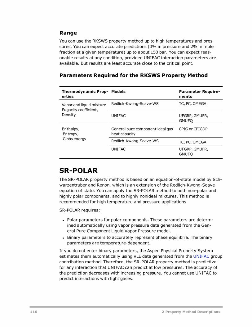
RangeYou can use the RKSWS property method up to high temperatures and pres-sures. You can expect accurate predictions (3% in pressure and 2% in molefraction at a given temperature) up to about 150 bar. You can expect reas-onable results at any condition, provided UNIFAC interaction parameters areavailable. But results are least accurate close to the critical point.
Parameters Required for the RKSWS Property Method
Thermodynamic Prop-erties
Models Parameter Require-ments
Vapor and liquidmixtureFugacity coefficient,Density
Redlich-Kwong-Soave-WS TC, PC, OMEGA
UNIFAC UFGRP, GMUFR,GMUFQ
Enthalpy,Entropy,Gibbs energy
General pure component ideal gasheat capacity
CPIG or CPIGDP
Redlich-Kwong-Soave-WS TC, PC, OMEGA
UNIFAC UFGRP, GMUFR,GMUFQ
SR-POLARThe SR-POLAR property method is based on an equation-of-state model by Sch-warzentruber and Renon, which is an extension of the Redlich-Kwong-Soaveequation of state. You can apply the SR-POLAR method to both non-polar andhighly polar components, and to highly nonideal mixtures. This method isrecommended for high temperature and pressure applications
SR-POLAR requires:
l Polar parameters for polar components. These parameters are determ-ined automatically using vapor pressure data generated from the Gen-eral Pure Component Liquid Vapor Pressure model.
l Binary parameters to accurately represent phase equilibria. The binaryparameters are temperature-dependent.
If you do not enter binary parameters, the Aspen Physical Property Systemestimates them automatically using VLE data generated from the UNIFAC groupcontribution method. Therefore, the SR-POLAR property method is predictivefor any interaction that UNIFAC can predict at low pressures. The accuracy ofthe prediction decreases with increasing pressure. You cannot use UNIFAC topredict interactions with light gases.
110 2 Property Method Descriptions
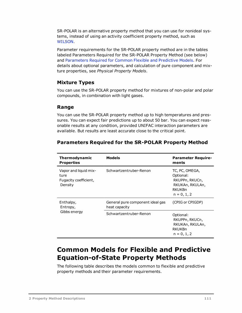
SR-POLAR is an alternative property method that you can use for nonideal sys-tems, instead of using an activity coefficient property method, such asWILSON.
Parameter requirements for the SR-POLAR property method are in the tableslabeled Parameters Required for the SR-POLAR Property Method (see below)and Parameters Required for Common Flexible and Predictive Models. Fordetails about optional parameters, and calculation of pure component and mix-ture properties, see Physical Property Models.
Mixture TypesYou can use the SR-POLAR property method for mixtures of non-polar and polarcompounds, in combination with light gases.
RangeYou can use the SR-POLAR property method up to high temperatures and pres-sures. You can expect fair predictions up to about 50 bar. You can expect reas-onable results at any condition, provided UNIFAC interaction parameters areavailable. But results are least accurate close to the critical point.
Parameters Required for the SR-POLAR Property Method
ThermodynamicProperties
Models Parameter Require-ments
Vapor and liquidmix-tureFugacity coefficient,Density
Schwartzentruber-Renon TC, PC, OMEGA,Optional:RKUPPn, RKUCn,RKUKAn, RKULAn,RKUKBnn = 0, 1, 2
Enthalpy,Entropy,Gibbs energy
General pure component ideal gasheat capacity
(CPIG or CPIGDP)
Schwartzentruber-Renon Optional:RKUPPn, RKUCn,RKUKAn, RKULAn,RKUKBnn = 0, 1, 2
Common Models for Flexible and PredictiveEquation-of-State Property MethodsThe following table describes the models common to flexible and predictiveproperty methods and their parameter requirements.
2 Property Method Descriptions 111

Parameters Required for Common Flexible and PredictiveModels
General
Property/Purpose Parameter Require-ments
Mass balance,Conversion Mass-basis↔Mole-basis
MW
Conversion Stdvol-basis↔Mole-basis VLSTD
Initialization of Flash calculations PLXANT
Using Free-water option: solubility of water inorganic phase
WATSOL
Enthalpy, enthalpy of reaction DHFORM
Gibbs energy of reaction DGFORM
Transport Properties
Property Models Parameter Require-ments
Vapor mixtureViscosity
Chung-Lee-Starling TC, PC, OMEGA
Thermal Con-ductivity
Chung-Lee-Starling TC, PC, OMEGA
Diffusivity Dawson-Khoury-Kobayashi MW, MUP, (STKPAR orLJPAR), VC
Surface tension General Pure Component Liquid Sur-face Tension
(TC, PC, OMEGA) orSIGDIP
LiquidmixtureViscosity
Chung-Lee-Starling TC, PC, OMEGA
Thermal Con-ductivity
Chung-Lee-Starling TC, PC, OMEGA
Diffusivity Wilke-Chang MW, VB
112 2 Property Method Descriptions
Liquid Activity Coefficient Prop-erty MethodsThe table labeled Liquid Activity Coefficient Property Methods (see Equations ofState) lists property methods for nonideal and strongly nonideal mixtures atlow pressures (maximum 10 atm). You can model permanent gases in liquidsolution using Henry's law. Binary parameters for many component pairs areavailable in the Aspen Physical Property System databanks. The UNIFAC basedproperty methods are predictive.
These property methods are not suited for electrolytes. In that case use an elec-trolyte activity coefficient property method. Model polar mixtures at high pres-sures with flexible and predictive equations of state. Non-polar mixtures aremore conveniently modeled with equations-of-state. Petroleum mixtures aremore accurately modeled with liquid fugacity correlations and equations ofstate.
In labeled Liquid Activity Coefficient Property Methods (see Equations of State)there are five different activity coefficient models and six different equation-of-state models. Each activity coefficient model is paired with a number of equa-tion-of-state models to form 26 property methods. The description of the prop-erty methods are therefore divided into two parts:
l Equation of statel Activity coefficient model
Each part discusses the characteristics of the specific model and its parameterrequirements. Parameters of the models occurring in all property methods aregiven in the table labeled Parameters Required for Common Models.
Equations of StateThis section discusses the characteristics and parameter requirements of thefollowing equations of state:
l Ideal gas lawl Redlich-Kwongl Nothnagell Hayden-O'Connelll HF equation of statel VPA/IK-CAPE Equation of State
2 Property Method Descriptions 113
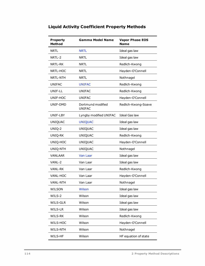
Liquid Activity Coefficient Property Methods
PropertyMethod
Gamma Model Name Vapor Phase EOSName
NRTL NRTL Ideal gas law
NRTL-2 NRTL Ideal gas law
NRTL-RK NRTL Redlich-Kwong
NRTL-HOC NRTL Hayden-O'Connell
NRTL-NTH NRTL Nothnagel
UNIFAC UNIFAC Redlich-Kwong
UNIF-LL UNIFAC Redlich-Kwong
UNIF-HOC UNIFAC Hayden-O'Connell
UNIF-DMD DortmundmodifiedUNIFAC
Redlich-Kwong-Soave
UNIF-LBY Lyngby modified UNIFAC Ideal Gas law
UNIQUAC UNIQUAC Ideal gas law
UNIQ-2 UNIQUAC Ideal gas law
UNIQ-RK UNIQUAC Redlich-Kwong
UNIQ-HOC UNIQUAC Hayden-O'Connell
UNIQ-NTH UNIQUAC Nothnagel
VANLAAR Van Laar Ideal gas law
VANL-2 Van Laar Ideal gas law
VANL-RK Van Laar Redlich-Kwong
VANL-HOC Van Laar Hayden-O'Connell
VANL-NTH Van Laar Nothnagel
WILSON Wilson Ideal gas law
WILS-2 Wilson Ideal gas law
WILS-GLR Wilson Ideal gas law
WILS-LR Wilson Ideal gas law
WILS-RK Wilson Redlich-Kwong
WILS-HOC Wilson Hayden-O'Connell
WILS-NTH Wilson Nothnagel
WILS-HF Wilson HF equation of state
114 2 Property Method Descriptions

Property Common Models
Vapor pressure General Pure Component Liquid Vapor Pressure
Liquidmolarvolume
Rackett
Heat of vapor-ization
General Pure Component Heat of Vaporization
Vapor viscosity General Pure Component Vapor Viscosity
Vapor thermal con-ductivity
General Pure Component Vapor Thermal Con-ductivity
Vapor diffusivity Dawson-Khoury-Kobayashi
Surface tension General Pure Component Liquid Surface Tension
Liquid viscosity General Pure Component Liquid Viscosity
Liquid thermal con-ductivity
General Pure Component Liquid Thermal Con-ductivity
Liquid diffusivity Wilke-Chang
Ideal Gas LawThe property methods that use the ideal gas law as the vapor phase model are:
l NRTLl NRTL-2l UNIF-LBYl UNIQUACl UNIQ-2l VANLAARl VANL-2l WILSONl WILS-2l WILS-GLRl WILS-LR
The ideal gas law is the simplest equation of state. It is also known as the com-bined laws of Boyle and Gay-Lussac.
Mixture TypesThe ideal gas law cannot model association behavior in the vapor phase, asoccurs with carboxylic acids. Choose Hayden-O'Connell or Nothnagel to modelthis behavior.
2 Property Method Descriptions 115
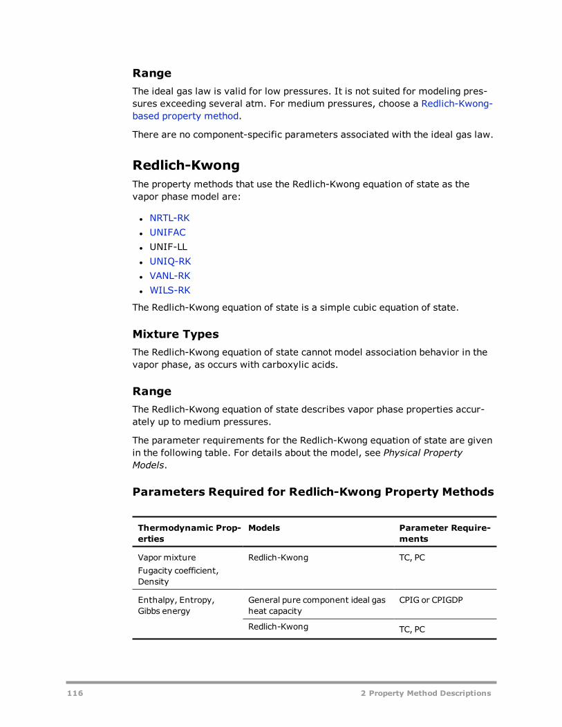
RangeThe ideal gas law is valid for low pressures. It is not suited for modeling pres-sures exceeding several atm. For medium pressures, choose a Redlich-Kwong-based property method.
There are no component-specific parameters associated with the ideal gas law.
Redlich-KwongThe property methods that use the Redlich-Kwong equation of state as thevapor phase model are:
l NRTL-RKl UNIFACl UNIF-LLl UNIQ-RKl VANL-RKl WILS-RK
The Redlich-Kwong equation of state is a simple cubic equation of state.
Mixture TypesThe Redlich-Kwong equation of state cannot model association behavior in thevapor phase, as occurs with carboxylic acids.
RangeThe Redlich-Kwong equation of state describes vapor phase properties accur-ately up to medium pressures.
The parameter requirements for the Redlich-Kwong equation of state are givenin the following table. For details about the model, see Physical PropertyModels.
Parameters Required for Redlich-Kwong Property Methods
Thermodynamic Prop-erties
Models Parameter Require-ments
Vapor mixtureFugacity coefficient,Density
Redlich-Kwong TC, PC
Enthalpy, Entropy,Gibbs energy
General pure component ideal gasheat capacity
CPIG or CPIGDP
Redlich-Kwong TC, PC
116 2 Property Method Descriptions
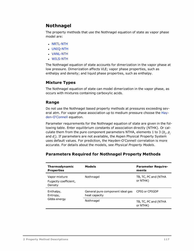
NothnagelThe property methods that use the Nothnagel equation of state as vapor phasemodel are:
l NRTL-NTHl UNIQ-NTHl VANL-NTHl WILS-NTH
The Nothnagel equation of state accounts for dimerization in the vapor phase atlow pressure. Dimerization affects VLE; vapor phase properties, such asenthalpy and density; and liquid phase properties, such as enthalpy.
Mixture TypesThe Nothnagel equation of state can model dimerization in the vapor phase, asoccurs with mixtures containing carboxylic acids.
RangeDo not use the Nothnagel based property methods at pressures exceeding sev-eral atm. For vapor phase association up to medium pressure choose the Hay-den-O'Connell equation.
Parameter requirements for the Nothnagel equation of state are given in the fol-lowing table. Enter equilibrium constants of association directly (NTHK). Or cal-culate them from the pure component parameters NTHA, elements 1 to 3 (bi, piand di). If parameters are not available, the Aspen Physical Property Systemuses default values. For prediction, the Hayden-O'Connell correlation is moreaccurate. For details about the models, see Physical Property Models.
Parameters Required for Nothnagel Property Methods
ThermodynamicProperties
Models Parameter Require-ments
Vapor mixtureFugacity coefficient,Density
Nothnagel TB, TC, PC and (NTHAor NTHK)
Enthalpy,Entropy,Gibbs energy
General pure component ideal gasheat capacity
CPIG or CPIGDP
Nothnagel TB, TC, PC and (NTHAor NTHK)
2 Property Method Descriptions 117

Hayden-O'ConnellThe property methods that use the Hayden-O'Connell equation of state as vaporphase model are:
l NRTL-HOCl UNIF-HOCl UNIQ-HOCl VANL-HOCl WILS-HOC
The Hayden-O'Connell equation of state predicts solvation and dimerization inthe vapor phase, up to medium pressure. Dimerization affects VLE; vaporphase properties, such as enthalpy and density; and liquid phase properties,such as enthalpy.
Mixture TypesThe Hayden-O'Connell equation reliably predicts solvation of polar compoundsand dimerization in the vapor phase, as occurs with mixtures containingcarboxylic acids.
RangeDo not use the Hayden-O'Connell-based property methods at pressures exceed-ing 10 to 15 atm.
Parameter requirements for the Hayden-O'Connell equation of state are givenin the following table. For details about the model, see Physical PropertyModels.
Parameters Required for Hayden-O'Connell Property Meth-ods
Thermodynamic Prop-erties
Models Parameter Require-ments
Vapor mixtureFugacity coefficient,Density
Hayden-O'Connell TC, PC, RGYR, MUP,HOCETA
Enthalpy,Entropy,Gibbs energy
General pure component ideal gasheat capacity
CPIG or CPIGDP
Hayden-O'Connell TC, PC, RGYR, MUP,HOCETA
HF Equation of State
118 2 Property Method Descriptions

The only property methods that use the HF equation of state as the vapor phasemodel are WILS-HF and ENRTL-HF.
For HF-hydrocarbon mixtures, the Wilson activity coefficient model is usuallybest suited for preventing nonrealistic liquid phase splitting.
The HF equation of state predicts the strong association of HF the vapor phaseat low pressures. Association (mainly hexamerization) affects VLE, vapor phaseproperties, such as enthalpy and density, and liquid phase properties, such asenthalpy.
Mixture TypesThe HF equation of state reliably predicts the strong association effects of HF ina mixture.
RangeDo not use the WILS-HF property method at pressures exceeding 3 atm.
Parameters for the HF equation of state are built-in for temperatures up to 373K. You can enter parameters and regress them using the Aspen Physical Prop-erty System Data Regression System (DRS), if necessary. For details about themodel, see Physical Property Models.
VPA/IK-CAPE Equation of StateThe VPA/IK-CAPE equation of state is similar to the HF equation of state butallows dimerization and tetramerization. No property method uses this equa-tion of state by default. It is recommended that this equation of state is used inplace of the HF equation of state with the WILS-HF and ENRTL-HF propertymethods, when dimerization and tetramerization is expected.
The main assumption of the model is that only molecular association causes thegas phase nonideality. Attractive forces between the molecules and the com-plexes are neglected.
There are three kinds of associations which can be modeled:
l Dimerization (examples: formic acid, acetic acid)l Tetramerization (example: acetic acid)l Hexamerization (example: hydrogen fluoride)
Mixture TypesThe VPA/IK-CAPE equation of state can be used to model strong associationeffects such as the presence of dimers, tetramers and hexamers. Use the VPAmodel for associating compounds like acids and hydrogen fluoride.
2 Property Method Descriptions 119
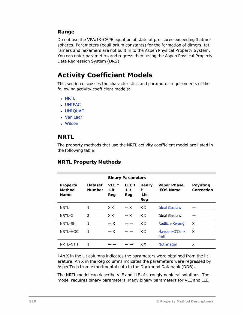
RangeDo not use the VPA/IK-CAPE equation of state at pressures exceeding 3 atmo-spheres. Parameters (equilibrium constants) for the formation of dimers, tet-ramers and hexamers are not built in to the Aspen Physical Property System.You can enter parameters and regress them using the Aspen Physical PropertyData Regression System (DRS)
Activity Coefficient ModelsThis section discusses the characteristics and parameter requirements of thefollowing activity coefficient models:
l NRTLl UNIFACl UNIQUACl Van Laarl Wilson
NRTLThe property methods that use the NRTL activity coefficient model are listed inthe following table:
NRTL Property Methods
Binary Parameters
PropertyMethodName
DatasetNumber
VLE †LitReg
LLE †LitReg
Henry†LitReg
Vapor PhaseEOS Name
PoyntingCorrection
NRTL 1 X X — X X X Ideal Gas law —
NRTL-2 2 X X — X X X Ideal Gas law —
NRTL-RK 1 — X — — X X Redlich-Kwong X
NRTL-HOC 1 — X — — X X Hayden-O'Con-nell
X
NRTL-NTH 1 — — — — X X Nothnagel X
†An X in the Lit columns indicates the parameters were obtained from the lit-erature. An X in the Reg columns indicates the parameters were regressed byAspenTech from experimental data in the Dortmund Databank (DDB).
The NRTL model can describe VLE and LLE of strongly nonideal solutions. Themodel requires binary parameters. Many binary parameters for VLE and LLE,
120 2 Property Method Descriptions

from literature and from regression of experimental data, are included in theAspen Physical Property System databanks. For details, see Aspen PhysicalProperty System Databanks in Physical Property Data in the help.
You can model the solubility of supercritical gases using Henry's law. Henrycoefficients are available in the Aspen Physical Property System databanks formany solutes with water and other solvents (see Aspen Physical Property Sys-tem Databanks in Physical Property Data in the help).
The property methods with a vapor phase model that can be used up to mod-erate pressures, have the Poynting correction included in the liquid fugacitycoefficient calculation. See the table labeled NRTL Property Methods (above) .
Heat of mixing is calculated using the NRTL model.
You can use separate data sets for the NRTL binary parameters to model prop-erties or equilibria at different conditions. It is also possible to use one data setfor VLE and a second data set for LLE (use NRTL and NRTL-2) property methodsare identical except for the data set number they use. For example, you canuse these property methods in different flowsheet sections or column sections.
Mixture TypesThe NRTL model can handle any combination of polar and non-polar com-pounds, up to very strong nonideality.
RangeParameters should be fitted in the temperature, pressure, and compositionrange of operation. No component should be close to its critical temperature.
Parameter requirements for the NRTL activity coefficient model are given in thefollowing table. For details about the model, see Physical Property Models.
Parameters Required for NRTL Property Methods
ThermodynamicProperties
Models Parameter Requirements
LiquidmixtureFugacity coefficient,Gibbs energy
NRTL liquid activity coef-ficient
NRTL
General Pure ComponentLiquid Vapor Pressure
PLXANT
Henry's constant Solvent: VC,Solute-solvent: HENRY
Brelvi-O'Connell Solvent: TC, PC, (ZC or RKTZRA),Solute: (VC or VLBROC)
2 Property Method Descriptions 121

ThermodynamicProperties
Models Parameter Requirements
Enthalpy,Entropy
General Pure ComponentIdeal Gas Heat Capacity
CPIG or CPIGDP
General Pure ComponentHeat of Vaporization
DHVLWT or DHVLDP
NRTL liquid activity coef-ficient
NRTL
Density Rackett TC, PC, (VC or VCRKT),(ZC or RKTZRA)
UNIFACUNIFAC is an activity coefficient model, like NRTL or UNIQUAC. But it is basedon group contributions, rather than molecular contributions. With a limited num-ber of group parameters and group-group interaction parameters, UNIFAC canpredict activity coefficients. The following table lists the property methodsbased on UNIFAC.
UNIFAC Property Methods
PropertyMethodName
ModelName
ParametersRev. Yr
Tmin/K
Tmax/K
HenryLitReg
VaporPhase EOSName
PoyntingCorrection
UNIFAC UNIFAC 5, 1991 290 420 X X Redlich-Kwong
X
UNIF-LL UNIFAC —, 1991 280 310 X X Redlich-Kwong
X
UNIF-HOC UNIFAC 5, 1991 290 420 X X Hayden-O'Connell
X
UNIF-DMD DMD-UNIF
1, 1993 290 420 X X Redlich-Kwong-Soave
X
UNIF-LBY LBY-UNIF
—, 1987 290 420 X X Ideal Gas law —
†An X in the Lit columns indicates the parameters were obtained from the lit-erature. An X in the Reg columns indicates the parameters were regressed byAspenTech from experimental data in the Dortmund Databank (DDB).
The original version of UNIFAC can predict VLE and LLE, using two sets of para-meters. So there are two property methods based on the original UNIFAC
122 2 Property Method Descriptions

model, one using the VLE data set (UNIFAC), the other using the LLE data set(UNIF-LL).
There are two modifications to the UNIFAC model. They are named after the loc-ation of the universities where they were developed: Lyngby in Denmark, andDortmund in Germany. The corresponding property methods are UNIF-LBY andUNIF-DMD. Both modifications:
l Include more temperature-dependent terms of the group-group inter-action parameters
l Predict VLE and LLE with a single set of parametersl Predict heats of mixing better
In the Dortmund modification, the prediction for activity coefficients at infinitedilution is improved.
You can model the solubility of supercritical gases using Henry's law. Henrycoefficients are available in the Aspen Physical Property System databanks formany solutes with water and other solvents (see Henry's Law Constants in Phys-ical Property Data).
The option sets with a vapor phase model that can be used up to moderate pres-sures, have the Poynting correction included in the liquid fugacity coefficient cal-culation (see the table labeled UNIFAC Property Methods above).
Heats of mixing are calculated using the UNIFAC or modified UNIFAC models.
Mixture TypesThe UNIFAC and modified UNIFAC models can handle any combination of polarand nonpolar compounds. Dissolved gas in solutions can be handled withHenry's Law. However, gas-solvent interactions are not predicted by UNIFAC.
RangeNo component should be close to its critical temperature. Approximate tem-perature ranges are indicated in the table labeled UNIFAC Property Methods(above).
The parameter sets for all UNIFAC models are regularly revised and extended.The table labeled UNIFAC Property Methods (above) gives the revision numbercurrently used in the Aspen Physical Property System. For details on the para-meters used, see Group Contribution Method Functional Groups in Physical Prop-erty Data.
The minimum parameter requirements for the UNIFAC and modified UNIFACmodels are given in the following table. For details about the models, see Phys-ical Property Models.
2 Property Method Descriptions 123
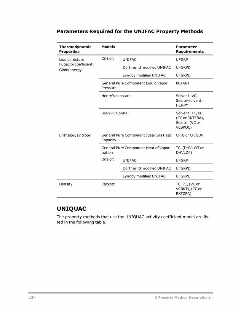
Parameters Required for the UNIFAC Property Methods
ThermodynamicProperties
Models ParameterRequirements
LiquidmixtureFugacity coefficient, Gibbs energy
One of: UNIFAC UFGRP
Dortmundmodified UNIFAC UFGRPD
Lyngby modified UNIFAC UFGRPL
General Pure Component Liquid VaporPressure
PLXANT
Henry's constant Solvent: VC,Solute-solvent:HENRY
Brelvi-O'Connell Solvent: TC, PC,(ZC or RKTZRA),Solute: (VC orVLBROC)
Enthalpy, Entropy General Pure Component Ideal Gas HeatCapacity
CPIG or CPIGDP
General Pure Component Heat of Vapor-ization
TC, (DHVLWT orDHVLDP)
One of: UNIFAC UFGRP
Dortmundmodified UNIFAC UFGRPD
Lyngby modified UNIFAC UFGRPL
Density Rackett TC, PC, (VC orVCRKT), (ZC orRKTZRA)
UNIQUACThe property methods that use the UNIQUAC activity coefficient model are lis-ted in the following table.
124 2 Property Method Descriptions

UNIQUAC Property Methods
Binary Parameters
PropertyMethodName
DatasetNumber
VLE †LitReg
LLE †LitReg
Henry†LitReg
Vapor PhaseEOS Name
PoyntingCorrection
UNIQUAC 1 X X X X X X Ideal Gas law —
UNIQ-2 2 X X X X X X Ideal Gas law —
UNIQ-RK 1 — X — — X X Redlich-Kwong X
UNIQ-HOC
1 — X — — X X Hayden-O'Connell X
UNIQ-NTH
1 — — — — X X Nothnagel X
†An X in the Lit columns indicates the parameters were obtained from the lit-erature. An X in the Reg columns indicates the parameters were regressed byAspenTech from experimental data in the Dortmund Databank (DDB).
The UNIQUAC model can describe strongly nonideal liquid solutions and liquid-liquid equilibria. The model requires binary parameters. Many binary para-meters for VLE and LLE, from literature and from regression of experimentaldata, are included in the Aspen Physical Property System databanks (fordetails, see Binary Parameters for Vapor-Liquid Applications in Physical Prop-erty Data in the help).
You can model the solubility of supercritical gases using Henry's law. Henrycoefficients are available from the databank (see Henry's Law Constants inPhysical Property Data in the help).
The property methods with a vapor phase model that can be used up to mod-erate pressures, have the Poynting correction included in the liquid fugacitycoefficient calculation (see the table labeled UNIQUAC Property Methodsabove).
Heats of mixing are calculated using the UNIQUAC model.
You can use separate data sets for the UNIQUAC binary parameters to modelproperties or equilibria at different conditions. It is also possible to use onedata set for VLE and a second data set for LLE (use UNIQUAC and UNIQ-2). Theproperty methods are identical except for the data set number they use. Forexample, you can use these options sets in different flowsheet sections orcolumn sections.
2 Property Method Descriptions 125

Mixture TypesThe UNIQUAC model can handle any combination of polar and non-polar com-pounds, up to very strong nonideality.
RangeParameters should be fitted in the temperature, pressure, and compositionrange of operation. No component should be close to its critical temperature.
Parameter requirements for the UNIQUAC activity coefficient model are givenin the following table. For details about the model, see Physical PropertyModels.
Parameters Required for UNIQUAC Property Methods
ThermodynamicProperties
Models Parameter Require-ments
LiquidmixtureFugacity coefficient, Gibbs energy
UNIQUAC liquid activity coef-ficient
GMUQR, GMUQQ, UNIQ
General Pure Component LiquidVapor Pressure
PLXANT
Henry's constant Solvent: VC,Solute-solvent: HENRY
Brelvi-O'Connell Solvent: TC, PC, (ZC orRKTZRA),Solute: (VC or VLBROC)
Enthalpy,Entropy
General Pure Component IdealGas Heat Capacity CPIG or CPIGDP
General Pure Component Heatof Vaporization
TC, (DHVLWT or DHVLDP)
UNIQUAC liquid activity coef-ficient
GMUQR, GMUQQ, UNIQ
Density Rackett TC, PC, (VC or VCRKT), (ZCor RKTZRA)
Van LaarThe property methods that use the Van Laar activity coefficient model are listedin the following table.
126 2 Property Method Descriptions

Van Laar Property Methods
Binary Parameters
PropertyMethodName
Datasetnumber
VLE †LitReg
LLE †LitReg
Henry†LitReg
Vapor PhaseEOS Name
PoyntingCorrection
VANLAAR 1 — — — — X X Ideal Gas law —
VANL-2 2 — — — — X X Ideal Gas law —
VANL-RK 1 — — — — X X Redlich-Kwong X
VANL-HOC
1 — — — — X X Hayden-O'Con-nell
X
VANL-NTH
1 — — — — X X Nothnagel X
†An X in the Lit columns indicates the parameters were obtained from the lit-erature. An X in the Reg columns indicates the parameters were regressed byAspenTech from experimental data in the Dortmund Databank (DDB).
The Van Laar model can describe nonideal liquid solutions with positive devi-ations from Raoult's law (see Activity Coefficient Method in Overview of AspenPhysical Property Methods). The model requires binary parameters.
You can model the solubility of supercritical gases using Henry's law. Henrycoefficients are available from the Aspen Physical Property System databank(see Henry's Law Constants in Physical Property Data in the help).
The property methods with a vapor phase model that can be used up to mod-erate pressures, have the Poynting correction included in the liquid fugacitycoefficient calculation (see the table labeled Van Laar Property Methods above).
Heats of mixing are calculated using the Van Laar model.
You can use separate data sets to model properties or equilibria at different con-ditions (use VANLAAR and VANL-2). The property methods are identical exceptfor the data set number they use. For example, you can use these propertymethods in different flowsheet or column sections.
Mixture TypesThe Van Laar model can handle any combination of polar and non-polar com-pounds with positive deviations from Raoult's law.
RangeParameters should be fitted in the temperature range of operation. No com-ponent should be close to its critical temperature.
2 Property Method Descriptions 127

Parameter requirements for the Van Laar activity coefficient model are given inthe following table. For details about the model, see Physical Property Models.
Parameters Required for Van Laar Property Methods
ThermodynamicProperties
Models Parameter Require-ments
LiquidmixtureFugacity coefficient, Gibbs energy
Van Laar liquid activity coef-ficient
VANL
General Pure Component LiquidVapor Pressure
PLXANT
Henry's constant Solvent: VC,Solute-solvent: HENRY
Brelvi-O'Connell Solvent: TC, PC, ( ZC orRKTZRA),Solute: (VC or VLBROC)
Enthalpy,Entropy
General Pure Component IdealGas Heat Capacity
CPIG or CPIGDP
General Pure Component Heatof Vaporization
TC, (DHVLWT or DHVLDP)
Van Laar liquid activity coef-ficient
VANL
Density Rackett TC, PC, (VC or VCRKT), (ZCor RKTZRA)
WilsonThe property methods that use the Wilson activity coefficient model or theWilson Model with Liquid Molar Volume are listed in the following table. OnlyWILS-VOL uses the latter model.
Wilson Property Methods
Binary Parameters
PropertyMethodName
Datasetnumber
VLELitReg
LLELitReg
HenryLitReg
Vapor PhaseEOS Name
PoyntingCorrection
WILSON 1 X X — — X X Ideal Gas law —
WILS-2 2 X X — — X X Ideal Gas law —
128 2 Property Method Descriptions

Binary Parameters
PropertyMethodName
Datasetnumber
VLELitReg
LLELitReg
HenryLitReg
Vapor PhaseEOS Name
PoyntingCorrection
WILS-GLR
1 X X — — X X Ideal Gas law —
WILS-LR 1 X X — — X X Ideal Gas law —
WILS-RK 1 — X — — X X Redlich-Kwong X
WILS-HOC
1 — X — — X X Hayden-O'Con-nell
X
WILS-NTH
1 — — — — X X Nothnagel X
WILS-HF 1 — — — — X X HF X
WILS-VOL
1 — — — — X X Redlich-Kwong X
†An X in the Lit columns indicates the parameters were obtained from the lit-erature. An X in the Reg columns indicates the parameters were regressed byAspenTech from experimental data in the Dortmund Databank (DDB).
The Wilson model can describe strongly nonideal liquid solutions. The modelcannot handle two liquid phases. In that case use NRTL or UNIQUAC. The modelrequires binary parameters. Many binary parameters for VLE, from literatureand from regression of experimental data, are included in the Aspen PhysicalProperty System databanks (for details, see Binary Parameters for VaporLiquid Applications in Physical Property Data in the help).
The solubility of supercritical gases can be modeled using Henry's law. Henrycoefficients are available from the databank for many solutes with water andother solvents (see Henry's Law Constants in Physical Property Data in thehelp).
The property methods with a vapor phase model that can be used up to mod-erate pressures, have the Poynting correction included in the liquid fugacitycoefficient calculation (see the table labeled Wilson Property Methods above).
Heats of mixing are calculated using the Wilson model.
You can use separate data sets for the Wilson binary parameters to model prop-erties or equilibria at different conditions (use WILSON and WILS-2). The prop-erty methods are identical except for the data set number they use. Forexample, you can use these property methods in different flowsheet or columnsections.
2 Property Method Descriptions 129

Mixture TypesThe Wilson model can handle any combination of polar and non-polar com-pounds, up to very strong nonideality.
RangeParameters should be fitted in the temperature, pressure, and compositionrange of operation. No component should be close to its critical temperature.
Parameter requirements for the Wilson activity coefficient model are given inthe table below. For details about the model, see Physical Property Models.
Parameters Required for the Wilson Property Methods
ThermodynamicProperties
Models Parameter Requirements
LiquidmixtureFugacity coefficient, Gibbs energy
Wilson liquid activity coef-ficient
WILSON
General Pure ComponentLiquid Vapor Pressure
PLXANT
Henry's constant Solvent: VC, Solute-solvent:HENRY
Brelvi-O'Connell Solvent: TC, PC, (ZC or RKTZRA),Solute: (VC or VLBROC)
Enthalpy,Entropy
General Pure ComponentIdeal Gas Heat Capacity
CPIG or CPIGDP
General Pure ComponentHeat of Vaporization
TC, (DHVLWT or DHVLDP)
Wilson liquid activity coef-ficient
WILSON
Density Rackett TC, PC, (VC or VCRKT), (ZC orRKTZRA)
Common Models for Liquid Activity Coef-ficient Property MethodsThe following table describes the models common to activity coefficient prop-erty methods and their parameter requirements.
130 2 Property Method Descriptions
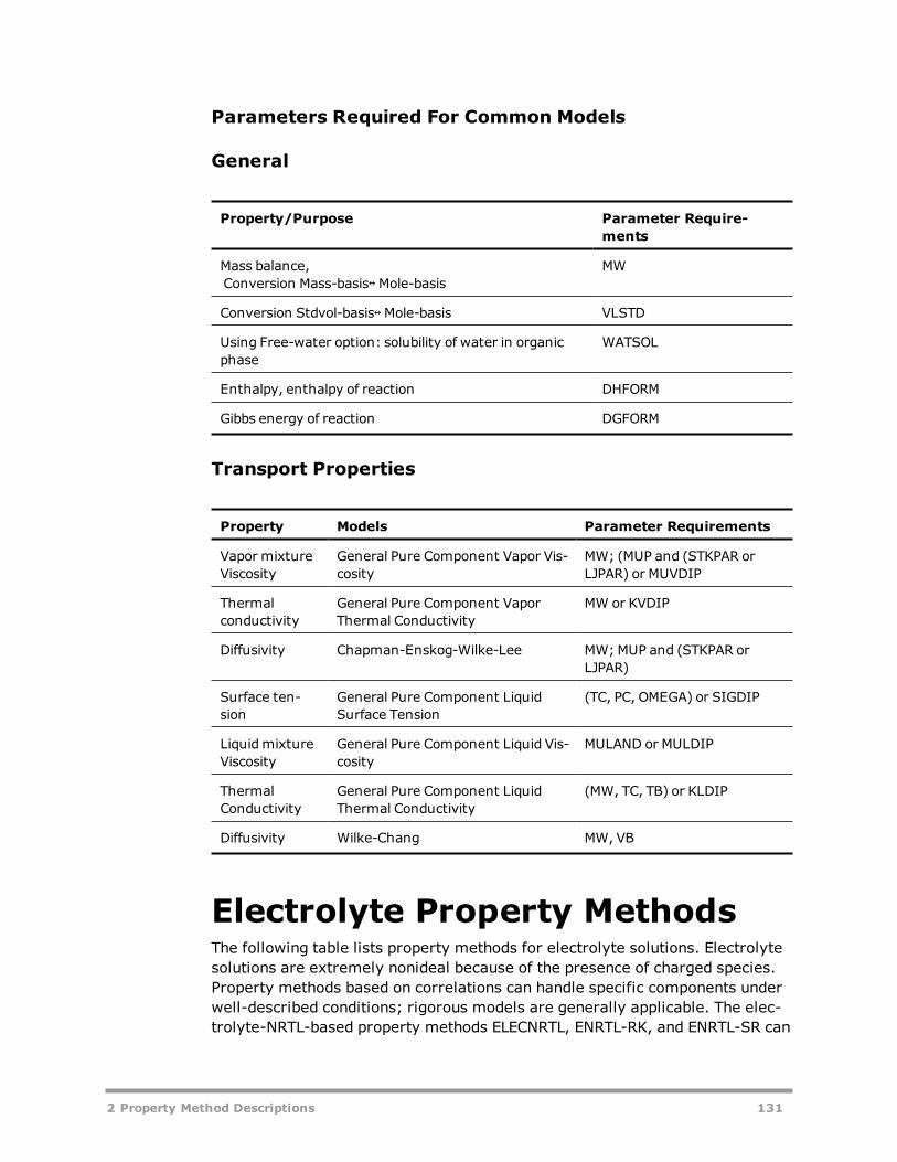
Parameters Required For Common Models
General
Property/Purpose Parameter Require-ments
Mass balance,Conversion Mass-basis↔Mole-basis
MW
Conversion Stdvol-basis↔Mole-basis VLSTD
Using Free-water option: solubility of water in organicphase
WATSOL
Enthalpy, enthalpy of reaction DHFORM
Gibbs energy of reaction DGFORM
Transport Properties
Property Models Parameter Requirements
Vapor mixtureViscosity
General Pure Component Vapor Vis-cosity
MW; (MUP and (STKPAR orLJPAR) or MUVDIP
Thermalconductivity
General Pure Component VaporThermal Conductivity
MW or KVDIP
Diffusivity Chapman-Enskog-Wilke-Lee MW;MUP and (STKPAR orLJPAR)
Surface ten-sion
General Pure Component LiquidSurface Tension
(TC, PC, OMEGA) or SIGDIP
LiquidmixtureViscosity
General Pure Component Liquid Vis-cosity
MULAND or MULDIP
ThermalConductivity
General Pure Component LiquidThermal Conductivity
(MW, TC, TB) or KLDIP
Diffusivity Wilke-Chang MW, VB
Electrolyte Property MethodsThe following table lists property methods for electrolyte solutions. Electrolytesolutions are extremely nonideal because of the presence of charged species.Property methods based on correlations can handle specific components underwell-described conditions; rigorous models are generally applicable. The elec-trolyte-NRTL-based property methods ELECNRTL, ENRTL-RK, and ENRTL-SR can
2 Property Method Descriptions 131
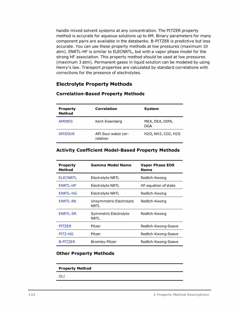
handle mixed solvent systems at any concentration. The PITZER propertymethod is accurate for aqueous solutions up to 6M. Binary parameters for manycomponent pairs are available in the databanks. B-PITZER is predictive but lessaccurate. You can use these property methods at low pressures (maximum 10atm). ENRTL-HF is similar to ELECNRTL, but with a vapor phase model for thestrong HF association. This property method should be used at low pressures(maximum 3 atm). Permanent gases in liquid solution can be modeled by usingHenry's law. Transport properties are calculated by standard correlations withcorrections for the presence of electrolytes.
Electrolyte Property Methods
Correlation-Based Property Methods
PropertyMethod
Correlation System
AMINES Kent-Eisenberg MEA, DEA, DIPA,DGA
APISOUR API Sour water cor-relation
H2O, NH3, CO2, H2S
Activity Coefficient Model-Based Property Methods
PropertyMethod
Gamma Model Name Vapor Phase EOSName
ELECNRTL Electrolyte NRTL Redlich-Kwong
ENRTL-HF Electrolyte NRTL HF equation of state
ENRTL-HG Electrolyte NRTL Redlich-Kwong
ENRTL-RK Unsymmetric ElectrolyteNRTL
Redlich-Kwong
ENRTL-SR Symmetric ElectrolyteNRTL
Redlich-Kwong
PITZER Pitzer Redlich-Kwong-Soave
PITZ-HG Pitzer Redlich-Kwong-Soave
B-PITZER Bromley-Pitzer Redlich-Kwong-Soave
Other Property Methods
Property Method
OLI
132 2 Property Method Descriptions

Common Models For Rigorous Property Methods
Property Model
Vapor pressure General Pure Component Liquid Vapor Pres-sure
Liquidmolar volume Rackett, Clarke
Heat of vaporization General Pure Component Heat of Vaporization
Infinite dilution heatcapacity
Criss-Cobble
Vapor viscosity General Pure Component Vapor Viscosity
Vapor thermal con-ductivity
General Pure Component Vapor Thermal Con-ductivity
Vapor diffusivity Dawson-Khoury-Kobayashi
Surface tension General Pure Component Liquid Surface Ten-sion, Onsager-Samaras
Liquid viscosity General Pure Component Liquid Viscosity,Jones-Dole
Liquid thermal con-ductivity
General Pure Component Liquid Thermal Con-ductivity, Riedel
Liquid diffusivity Wilke-Chang, Nernst-Hartley
Do not use the electrolyte property methods for nonelectrolyte systems. SeeClassification of Property Methods and Recommended Use for more help.
For general thermodynamic principles, see Electrolyte Models in Overview ofAspen Physical Property Methods. The Electrolyte Calculation section containsspecifics on electrolyte calculation. For details on methods, see Property Cal-culation Methods and Routes. The property method descriptions give the min-imum parameter requirements for the thermodynamic property models used,also of the common thermodynamic property models. The general and trans-port property parameter requirements for coefficient-based property methodsare in the table labeled Parameters Required for General and Transport Models.For details on models, see Physical Property Models.
AMINESThe AMINES property method uses the Kent-Eisenberg method for K-values andenthalpy. It is designed for systems containing water, one of four eth-anolamines, hydrogen sulfide, carbon dioxide, and other components typicallypresent in gas-sweetening processes. It can be used for the following fouramines:
2 Property Method Descriptions 133
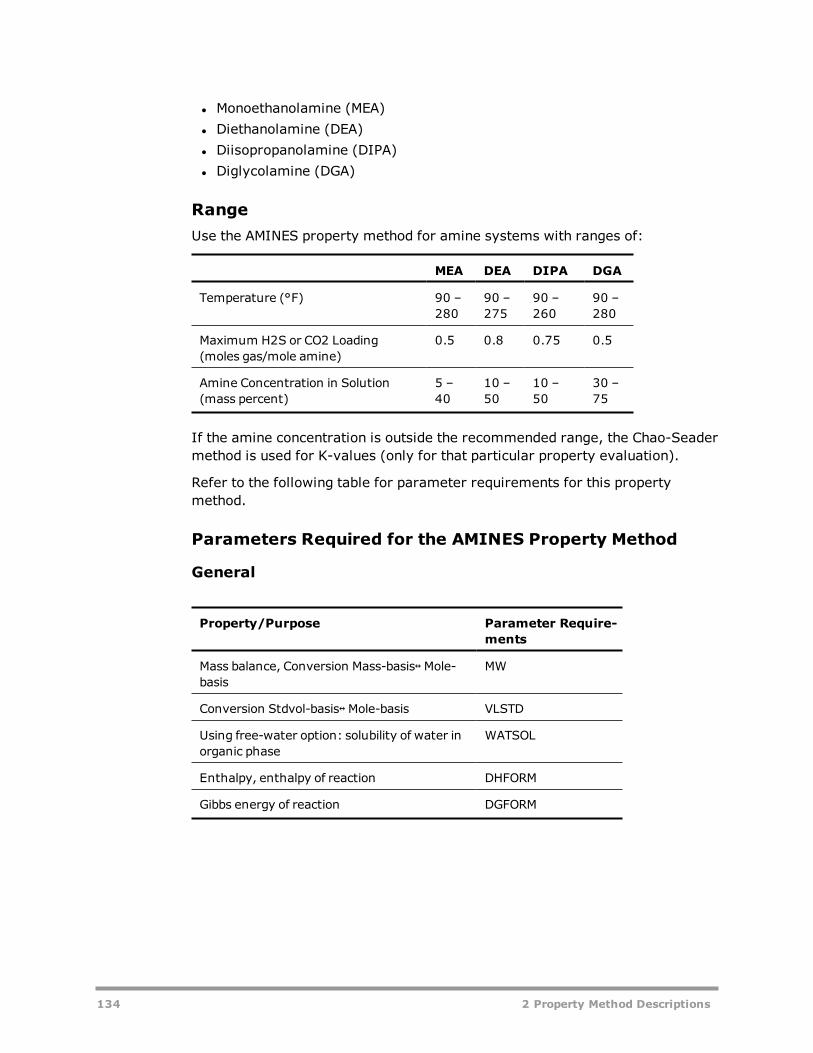
l Monoethanolamine (MEA)l Diethanolamine (DEA)l Diisopropanolamine (DIPA)l Diglycolamine (DGA)
RangeUse the AMINES property method for amine systems with ranges of:
MEA DEA DIPA DGA
Temperature (°F) 90 –280
90 –275
90 –260
90 –280
Maximum H2S or CO2 Loading(moles gas/mole amine)
0.5 0.8 0.75 0.5
Amine Concentration in Solution(mass percent)
5 –40
10 –50
10 –50
30 –75
If the amine concentration is outside the recommended range, the Chao-Seadermethod is used for K-values (only for that particular property evaluation).
Refer to the following table for parameter requirements for this propertymethod.
Parameters Required for the AMINES Property Method
General
Property/Purpose Parameter Require-ments
Mass balance, Conversion Mass-basis↔Mole-basis
MW
Conversion Stdvol-basis↔Mole-basis VLSTD
Using free-water option: solubility of water inorganic phase
WATSOL
Enthalpy, enthalpy of reaction DHFORM
Gibbs energy of reaction DGFORM
134 2 Property Method Descriptions
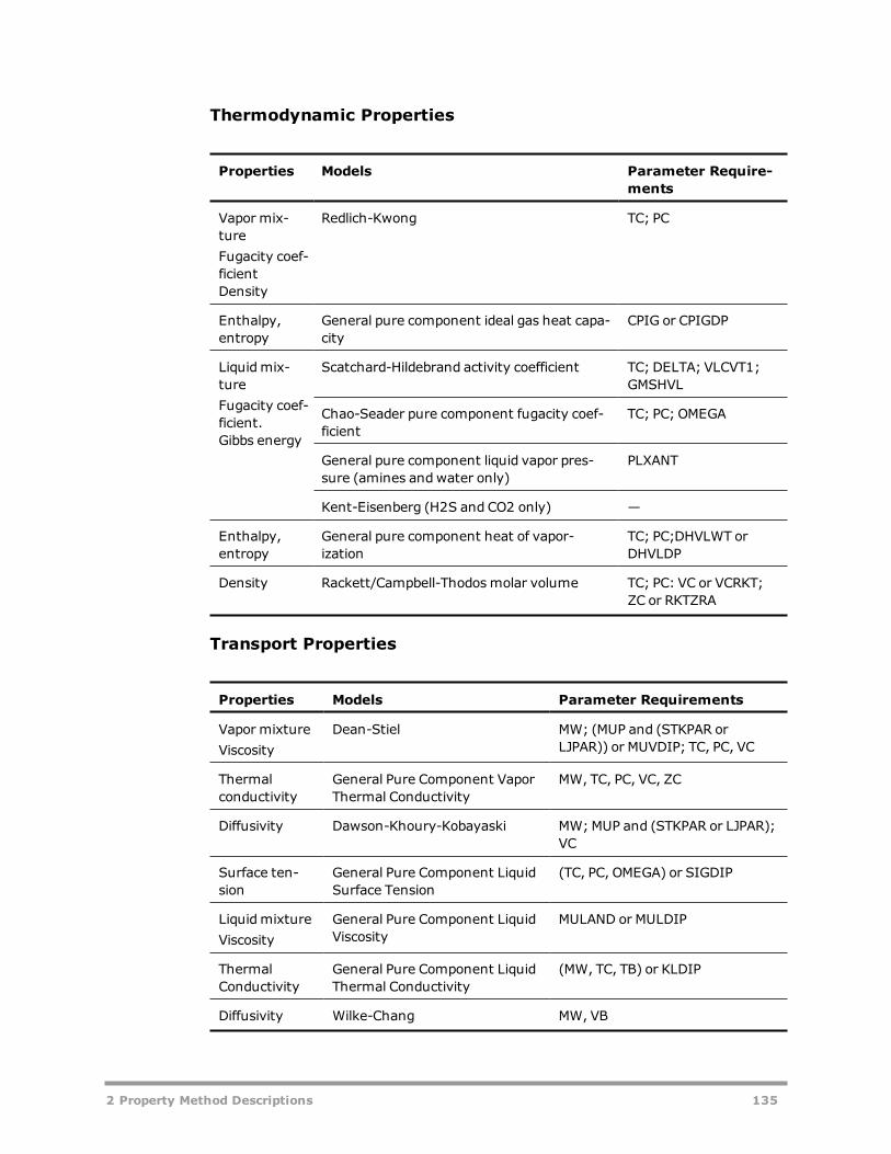
Thermodynamic Properties
Properties Models Parameter Require-ments
Vapor mix-tureFugacity coef-ficientDensity
Redlich-Kwong TC; PC
Enthalpy,entropy
General pure component ideal gas heat capa-city
CPIG or CPIGDP
Liquidmix-tureFugacity coef-ficient.Gibbs energy
Scatchard-Hildebrand activity coefficient TC; DELTA; VLCVT1;GMSHVL
Chao-Seader pure component fugacity coef-ficient
TC; PC; OMEGA
General pure component liquid vapor pres-sure (amines andwater only)
PLXANT
Kent-Eisenberg (H2S and CO2 only) —
Enthalpy,entropy
General pure component heat of vapor-ization
TC; PC;DHVLWT orDHVLDP
Density Rackett/Campbell-Thodosmolar volume TC; PC: VC or VCRKT;ZC or RKTZRA
Transport Properties
Properties Models Parameter Requirements
Vapor mixtureViscosity
Dean-Stiel MW; (MUP and (STKPAR orLJPAR)) or MUVDIP; TC, PC, VC
Thermalconductivity
General Pure Component VaporThermal Conductivity
MW, TC, PC, VC, ZC
Diffusivity Dawson-Khoury-Kobayaski MW;MUP and (STKPAR or LJPAR);VC
Surface ten-sion
General Pure Component LiquidSurface Tension
(TC, PC, OMEGA) or SIGDIP
LiquidmixtureViscosity
General Pure Component LiquidViscosity
MULAND or MULDIP
ThermalConductivity
General Pure Component LiquidThermal Conductivity
(MW, TC, TB) or KLDIP
Diffusivity Wilke-Chang MW, VB
2 Property Method Descriptions 135

APISOURThe APISOUR property method:
l Uses the API procedure for K-values and enthalpy of sour water sys-tems.
l Is designed for sour water systems containing primarily water, ammo-nia, hydrogen sulfide and carbon dioxide.
l Is applicable in the temperature range of 20 – 140°C.l Has an overall average error between measured and predicted partialpressures of about 30% for ammonia, carbon dioxide, and hydrogen sulf-ide.
l Does not require any user-supplied parameters.l Is recommended for fast calculation of sour water systems at limitedconcentration. For more accurate results, use the ELECNRTL propertymethod.
l Does not depend on any CHEMISTRY input. Do not specify Chemistry IDin any Electrolyte calculation options field.
Note: APISOUR uses an activity coefficient method such as NRTL or Wilson to calculatefugacity coefficients for components other than water, ammonia, hydrogen sulfide, or car-bon dioxide. To specify this method, on theMethods| Selected Methods | APISOUR |Models sheet, select a model for calculating gamma. The default is GMRENON which usesNRTL.
Parameter requirements for the APISOUR property method are listed in the fol-lowing table.
Parameters Required for the APISOUR Property Method
General
Property/Purpose Parameter Require-ments
Mass balance, Conversion Mass-basis↔Mole-basis MW
Conversion Stdvol-basis↔Mole-basis VLSTD
Using Free-water option: solubility of water in organicphase
WATSOL
Enthalpy, enthalpy of reaction DHFORM
Gibbs energy of reaction DGFORM
136 2 Property Method Descriptions

Transport Properties
Properties Models Parameter Requirements
Vapor mixtureViscosity
General Pure Component VaporViscosity
MW; (MUP and (STKPAR orLJPAR)) or MUVDIP
Thermalconductivity
General Pure Component VaporThermal Conductivity
MW or KVDIP
Diffusivity Chapman-Enskog-Wilke-Lee MW;MUP and (STKPAR or LJPAR)
Surface tension General Pure Component LiquidSurface Tension
(TC, PC, OMEGA) or SIGDIP
LiquidmixtureViscosity
General Pure Component LiquidViscosity
MULAND or MULDIP
ThermalConductivity
General Pure Component LiquidThermal Conductivity
(MW, TC, TB) or KLDIP
Diffusivity Wilke-Chang MW, VB
ELECNRTLThe ELECNRTL property method is the most versatile electrolyte propertymethod. It can handle very low and very high concentrations. It can handleaqueous and mixed solvent systems.
The ELECNRTL is fully consistent with the NRTL-RK property method: themolecular interactions are calculated exactly the same way, thereforeELECNRTL can use the databank for binary molecular interaction parameters forthe NRTL-RK property method.
Many binary and pair parameters and chemical equilibrium constants fromregression of experimental data are included in Aspen Physical Property Sys-tem databanks. See Electrolytes Data in Physical Property Data in the help, fordetails on the systems included, the sources of the data, and the ranges ofapplication.
The solubility of supercritical gases can be modeled using Henry's law. Henrycoefficients are available from the databank (see Activity Coefficient Method inOverview of Aspen Physical Property Methods).
Heats of mixing are calculated using the electrolyte NRTL model.
The Redlich-Kwong equation of state is used for all vapor phase properties,which cannot model association behavior in the vapor phase as occurs withcarboxylic acids or HF. For carboxylic acids, choose Hayden-O'Connell or Noth-nagel; for HF choose ENRTL-HF.
2 Property Method Descriptions 137

Mixture TypesAny liquid electrolyte solution unless there is association in the vapor phase.
RangeVapor phase properties are described accurately up to medium pressures. Inter-action parameters should be fitted in the range of operation.
The parameter requirements for the ELECNRTL property method are given inthe following table, and in Parameters Required for General and Transport Prop-erty Models. For details about the model see Physical Property Models.
Parameters Required for the ELECNRTL Property Method
ThermodynamicProperties
Models Parameter Requirements
Vapor mixtureFugacity coefficient,Density
Redlich-Kwong TC, PC
Enthalpy,Entropy,Gibbs energy
General pure component idealgas heat capacity correlation
CPIG or CPIGDP orCPIXP1, CPIXP2, CPIXP3
Redlich-Kwong TC, PC
LiquidmixtureFugacity coefficient,Gibbs energy
Electrolyte NRTL Mol.: CPDIECIon: RADIUSMol.-Mol.: NRTLMol.-Ion, Ion-Ion: GMELCC,GMELCDGMELCE, GMELCN
General Pure ComponentLiquid Vapor Pressure
PLXANT
Henry's constant Solvent: VC, Mol. solute-solvent: HENRY
Brelvi-O'Connell Solvent: TC, PC, (ZC orRKTZRA), Mol. solute: (VC orVLBROC)
138 2 Property Method Descriptions
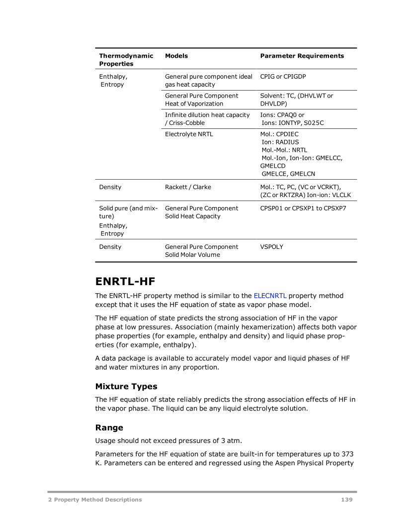
ThermodynamicProperties
Models Parameter Requirements
Enthalpy,Entropy
General pure component idealgas heat capacity
CPIG or CPIGDP
General Pure ComponentHeat of Vaporization
Solvent: TC, (DHVLWT orDHVLDP)
Infinite dilution heat capacity/ Criss-Cobble
Ions: CPAQ0 orIons: IONTYP, S025C
Electrolyte NRTL Mol.: CPDIECIon: RADIUSMol.-Mol.: NRTLMol.-Ion, Ion-Ion: GMELCC,GMELCDGMELCE, GMELCN
Density Rackett / Clarke Mol.: TC, PC, (VC or VCRKT),(ZC or RKTZRA) Ion-ion: VLCLK
Solid pure (andmix-ture)Enthalpy,Entropy
General Pure ComponentSolid Heat Capacity
CPSP01 or CPSXP1 to CPSXP7
Density General Pure ComponentSolid Molar Volume
VSPOLY
ENRTL-HFThe ENRTL-HF property method is similar to the ELECNRTL property methodexcept that it uses the HF equation of state as vapor phase model.
The HF equation of state predicts the strong association of HF in the vaporphase at low pressures. Association (mainly hexamerization) affects both vaporphase properties (for example, enthalpy and density) and liquid phase prop-erties (for example, enthalpy).
A data package is available to accurately model vapor and liquid phases of HFand water mixtures in any proportion.
Mixture TypesThe HF equation of state reliably predicts the strong association effects of HF inthe vapor phase. The liquid can be any liquid electrolyte solution.
RangeUsage should not exceed pressures of 3 atm.
Parameters for the HF equation of state are built-in for temperatures up to 373K. Parameters can be entered and regressed using the Aspen Physical Property
2 Property Method Descriptions 139
Data Regression System (DRS) if needed. For details about the model, see Elec-trolyte NRTL Activity Coefficient Model in Physical Property Models. For theparameter requirements for the electrolyte NRTL model, see the table labeledParameters Required for the ELECNRTL Property Method (see ELECNRTL). Forgeneral and transport property parameter requirements, see the table Para-meters Required for General and Transport Property Models.
ENRTL-HGThe ENRTL-HG property method is similar to the ELECNRTL property method,except it uses the Helgeson model for standard properties calculations. The Hel-geson model is a very accurate and flexible equation of state that calculatesstandard enthalpy, entropy, Gibbs free energy and volume for components inaqueous solutions. The Helgeson model should provide more accurate enthalpyand Gibbs free energy of process streams up to high temperatures and pres-sures. The model is also used to calculate Gibbs free energy for use in estim-ating chemical equilibrium constants (for both equilibrium and salt precipitationreactions) when they are missing. Equilibrium constants calculated using theHelgeson model have been found to be reasonably accurate and extrapolatewell with respect to temperature.
Mixture TypesAny liquid electrolyte solution is acceptable, unless there is association in thevapor phase.
RangeVapor phase properties are described accurately up to medium pressures. Inter-action parameters should be fitted in the range of operation.
For parameter requirements for the electrolyte NRTL model, see the tablelabeled Parameters Required for the ELECNRTL Property Method (seeELECNRTL). For general and transport property parameter requirements, seethe table labeled Parameters Required for General and Transport PropertyModels.
ENRTL-RKThe ENRTL-RK property method is based on the Unsymmetric Electrolyte NRTLproperty model. It uses:
l The Redlich-Kwong equation of state for vapor phase propertiesl The unsymmetric reference state (infinite dilution in aqueous solution)for ionic species.
l Henry's law for solubility of supercritical gases.l Unsymmetric Electrolyte NRTL method of handling zwitterions
140 2 Property Method Descriptions

ENRTL-RK reduces to the NRTL-RK property method when there are no ions inthe system.
The ENRTL-RK method is identical to ELECNRTL for systems containing a singleelectrolyte. However, for mixed electrolyte systems, the ENRTL-RK methoduses the mixing rules only to calculate interaction parameters, instead of cal-culating both interaction parameters and Gibbs free energy from mixing rules.Furthermore, the ENRTL-RK uses a single thermodynamics framework to cal-culate the activity coefficients, Gibbs free energy and enthalpy, instead of usingseparate models as in ELECNRTL.
Mixture TypesAny liquid electrolyte solution containing water, unless there is association inthe vapor phase.
RangeVapor phase properties are described accurately up to medium pressures. Inter-action parameters should be fitted in the range of operation.
The parameter requirements for the ENRTL-RK property method are given inthe following table, and in Parameters Required for General and Transport Prop-erty Models. For details about the model see Physical Property Models.
Parameters Required for the ENRTL-RK Property Method
ThermodynamicProperties
Models Parameter Requirements
Vapor mixtureFugacity coefficient,Density
Redlich-Kwong TC, PC
Enthalpy,Entropy,Gibbs energy
General pure component idealgas heat capacity correlation
CPIG or CPIGDP orCPIXP1, CPIXP2, CPIXP3
Redlich-Kwong TC, PC
2 Property Method Descriptions 141

ThermodynamicProperties
Models Parameter Requirements
LiquidmixtureFugacity coefficient,Gibbs energy,Enthalpy, Entropy
Unsymmetric electrolyteNRTL
Mol.: CPDIECIon: RADIUSMol.-Mol.: NRTLMol.-Ion, Ion-Ion: GMENCC,GMENCD, GMENCE, GMENCN
General Pure ComponentLiquid Vapor Pressure
PLXANT
Henry's constant Solvent: VC, Mol. solute-solvent: HENRY
Brelvi-O'Connell Solvent: TC, PC, (ZC orRKTZRA), Mol. solute: (VC orVLBROC)
Enthalpy,Entropy
General pure component idealgas heat capacity
CPIG or CPIGDP
General Pure ComponentHeat of Vaporization
Solvent: TC, (DHVLWT orDHVLDP)
Infinite dilution heat capacity/ Criss-Cobble
Ions: CPAQ0 orIons: IONTYP, S025C
Density Rackett / Clarke Mol.: TC, PC, (VC or VCRKT),(ZC or RKTZRA) Ion-ion: VLCLK
Solid pure (andmix-ture)Enthalpy,Entropy
General Pure ComponentSolid Heat Capacity
CPSP01 or CPSXP1 to CPSXP7
Density General Pure ComponentSolid Molar Volume
VSPOLY
ENRTL-SRThe ENRTL-SR property method is based on the Symmetric Electrolyte NRTLproperty model. It uses:
l The Redlich-Kwong equation of state vapor phase propertiesl The symmetric reference state (pure fused salts) for ionic species.l Henry's law for solubility of supercritical gases.l Symmetric Electrolyte NRTL method of handling zwitterions
ENRTL-SR reduces to the NRTL-RK property method when there are no ions inthe system.
ENRTL-SR uses a single thermodynamics framework to calculate the activitycoefficients, Gibbs free energy, enthalpy, and entropy.
142 2 Property Method Descriptions

When using this property method, you must specify the Symmetric basis foractivity coefficients of Ionic components on the Input | Specificationssheet of the Chemistry block it is used with.
Mixture TypesAny liquid electrolyte solution unless there is association in the vapor phase.
RangeVapor phase properties are described accurately up to medium pressures. Inter-action parameters should be fitted in the range of operation.
The parameter requirements for the ENRTL-SR property method are given inthe following table, and in Parameters Required for General and Transport Prop-erty Models. For details about the model see Physical Property Models.
Parameters Required for the ENRTL-SR Property Method
ThermodynamicProperties
Models Parameter Requirements
Vapor mixtureFugacity coefficient,Density
Redlich-Kwong TC, PC
Enthalpy,Entropy,Gibbs energy
General pure component idealgas heat capacity correlation
CPIG or CPIGDP orCPIXP1, CPIXP2, CPIXP3
Redlich-Kwong TC, PC
LiquidmixtureFugacity coefficient,Gibbs energy,Enthalpy, Entropy
Symmetric electrolyte NRTL Mol.: CPDIECIon: RADIUSMol.-Mol.: NRTLMol.-Ion, Ion-Ion: GMENCC,GMENCD, GMENCE, GMENCN
General Pure ComponentLiquid Vapor Pressure
PLXANT
Henry's constant Solvent: VC, Mol. solute-solvent: HENRY
Brelvi-O'Connell Solvent: TC, PC, (ZC orRKTZRA), Mol. solute: (VC orVLBROC)
2 Property Method Descriptions 143

ThermodynamicProperties
Models Parameter Requirements
Enthalpy,Entropy
General pure component idealgas heat capacity
CPIG or CPIGDP
General Pure ComponentHeat of Vaporization
Solvent: TC, (DHVLWT orDHVLDP)
Infinite dilution heat capacity/ Criss-Cobble
Ions: CPAQ0 orIons: IONTYP, S025C
Density Rackett / Clarke Mol.: TC, PC, (VC or VCRKT),(ZC or RKTZRA) Ion-ion: VLCLK
Solid pure (andmix-ture)Enthalpy,Entropy
General Pure ComponentSolid Heat Capacity
CPSP01 or CPSXP1 to CPSXP7
Density General Pure ComponentSolid Molar Volume
VSPOLY
PITZERThe PITZER property method is based on an aqueous electrolyte activity coef-ficient model. It has no overlap with other activity coefficient models. It canaccurately calculate the behavior of aqueous electrolyte solutions with orwithout molecular solutes up to 6 molal ionic strength.
Many interaction parameters from regression of experimental data are includedin databanks and data packages (for details, see Overview of Aspen PhysicalProperty Methods).
You can model the solubility of supercritical gases using Henry's law. Henrycoefficients are available from the Aspen Physical Property System databanks(see Overview of Aspen Physical Property Methods).
Heats of mixing are calculated using the Pitzer model.
The Redlich-Kwong-Soave equation of state is used for the vapor phase fugacitycoefficient. All other vapor phase properties are assumed ideal. Redlich-Kwong-Soave cannot model association behavior in the vapor phase (forexample, carboxylic acids or HF). For carboxylic acids, choose a non-elec-trolyte activity coefficient model with Hayden-O'Connell or Nothnagel; for HFchoose ENRTL-HF or WILS-HF.
Mixture TypesYou can use the Pitzer model for any aqueous electrolyte solution up to 6 molalionic strength, not showing association in the vapor phase.
144 2 Property Method Descriptions

Important: PITZER cannot be used for systems with any other solvent or mixedsolvents. Any non-water molecular components are considered solutes and treated asHenry components.
RangeVapor phase fugacities are described accurately up to medium pressures. Inter-action parameters should be fitted in the range of operation.
The parameter requirements for the PITZER property method are given in thefollowing table, and the table labeled Parameters Required for General andTransport Property Models. For details about the model, see Physical PropertyModels.
Parameters Required for the PITZER Property Method
ThermodynamicProperties
Models Parameter Requirements
Vapor mixtureFugacity coefficient,Density
Redlich-Kwong-Soave TC, PC, OMEGA
Enthalpy,Entropy,Gibbs energy
General pure componentideal gas heat capacity cor-relation
CPIG or CPIGDP orCPIXP1, CPIXP2, CPIXP3
Redlich-Kwong TC, PC, OMEGA
LiquidmixtureFugacity coefficient,Gibbs energy
Pitzer Cation-anion: GMPTB0, GMPTB1,GMPTB2, GMPTB3, GMPTCCation-cation: GMPTTHAnion-anion: GMPTTHCation1-cation2-commonanion: GMPTPSAnion1-anion2-common cation:GMPTPSMolecule-ion, Mol. – Mol.:GMPTB0, GMPTB1, GMPTC
General Pure ComponentLiquid Vapor Pressure
PLXANT
Henry's constant Solvent: VC, Mol. solute-solvent:HENRY
Brelvi-O'Connell Solvent: TC, PC, (ZC or RKTZRA),Mol. solute: (VC or VLBROC)
2 Property Method Descriptions 145

ThermodynamicProperties
Models Parameter Requirements
Enthalpy,Entropy
General pure componentideal gas heat capacity
CPIG or CPIGDP
General Pure ComponentHeat of Vaporization
Solvent: TC, (DHVLWT orDHVLDP)
Infinite dilution heat capa-city / Criss-Cobble
Ions: CPAQ0 orIons: IONTYP, S025C
Pitzer Cation-anion: GMPTB0, GMPTB1,GMPTB2, GMPTB3, GMPTCCation-cation: GMPTTHAnion-anion: GMPTTHCation1-cation2-commonanion: GMPTPSAnion1-anion2-common cation:GMPTPSMolecule-ion, Mol. – Mol.:GMPTB0,GMPTB1,GMPTC
Density Rackett / Clarke Mol.: TC, PC, (VC or VCRKT), (ZCor RKTZRA) Ion-ion: VLCLK
Solid pure (andmix-ture)Enthalpy,Entropy
General Pure ComponentSolid Heat Capacity
CPSP01 orCPSXP1 to CPSXP7
Density General Pure ComponentSolid Molar Volume
VSPOLY
B-PITZERThe B-PITZER property method is based on the simplified Pitzer aqueous elec-trolyte activity coefficient model, which neglects third order interactions. It canpredict the behavior of aqueous electrolyte solutions up to 6 molal ionicstrength. It is not as accurate as ELECNRTL or PITZER with fitted parameters.But, it is better than using these property methods without interaction para-meters.
You can model the solubility of supercritical gases using Henry's law. Henrycoefficients are available from the Aspen Physical Property System databanks(see Overview of Aspen Physical Property Methods).
Heats of mixing are calculated using the Bromley-Pitzer model.
The Redlich-Kwong-Soave equation of state is used for the vapor phase fugacitycoefficient. All other vapor phase properties are assumed ideal. Redlich-Kwong-Soave cannot model association behavior in the vapor phase (forexample with carboxylic acids or HF). For carboxylic acids, choose a non-
146 2 Property Method Descriptions

electrolyte activity coefficient model with Hayden-O'Connell or Nothnagel; forHF choose ENRTL-HF or WILS-HF.
Mixture TypesYou can use the B-PITZER model for any aqueous electrolyte solution up to 6Mionic strength, not showing association in the vapor phase.
RangeVapor phase fugacities are described accurately up to medium pressures. Inter-action parameters should be fitted in the range of operation.
The parameter requirements for the B-PITZER property method are given in thefollowing table, and the table labeled Parameters Required for General andTransport Property Models. For details about the model, see Pitzer Activity Coef-ficient Model in Physical Property Models.
Parameters Required for the B-PITZER Property Method
ThermodynamicProperties
Models Parameter Requirements
Vapor mixtureFugacitycoefficient, Density
Redlich-Kwong-Soave TC, PC, OMEGA
Enthalpy,Entropy,Gibbs energy
General pure component idealgas heat capacity correlation
CPIG or CPIGDP or CPIXP1,CPIXP2, CPIXP3
Redlich-Kwong TC, PC, OMEGA
LiquidmixtureFugacity coef-ficient,Gibbs energy
Bromley-Pitzer Ionic: GMBPB, GMBPD Optional:Cation-anion: GMPTB0,GMPTB1, GMPTB2, GMPTB3Cation-cation: GMPTTHAnion-anion: GMPTTHMolecule-ion, Mol.-Mol.:GMPTB0, GMPTB1
General Pure ComponentLiquid Vapor Pressure
PLXANT
Henry's constant Solvent: VC, Mol. solute-solvent: HENRY
Brelvi-O'Connell Solvent: TC, PC, (ZC orRKTZRA), Mol. solute: (VC orVLBROC)
2 Property Method Descriptions 147

ThermodynamicProperties
Models Parameter Requirements
Enthalpy,Entropy
General pure component idealgas heat capacity
CPIG or CPIGDP
General Pure Component Heatof Vaporization
Solvent: TC, (DHVLWT orDHVLDP)
Infinite dilution heat capacity /Criss-Cobble
Ions: CPAQ0 orIons: IONTYP, S025C
Bromley-Pitzer Ionic: GMBPB, GMBPDOptional:Cation-anion: GMPTB0,GMPTB1, GMPTB2, GMPTB3Cation-cation:GMPTTHAnion-anion: GMPTTHMolecule-ion, Mol.-Mol.:GMPTB0, GMPTB1
Density Rackett / Clarke Mol.: TC, PC, (VC or VCRKT), (ZCor RKTZRA) Ion-ion: VLCLK
Solid pure (andmixture)Enthalpy,Entropy
General Pure Component SolidHeat Capacity
CPSP01 or CPSXP1 to CPSXP7
Density General Pure Component SolidMolar Volume
VSPOLY
PITZ-HGThe PITZ-HG property method is similar to the PITZER property method, exceptit uses the Helgeson model for standard properties calculations. The Helgesonmodel is a very accurate and flexible equation of state that calculates standardenthalpy, entropy, Gibbs free energy and volume for components in aqueoussolutions. The Helgeson model should provide more accurate enthalpy andGibbs free energy of process streams up to high temperatures and pressures.The Helgeson model is also used to calculate Gibbs free energy for use in estim-ating chemical equilibrium constants (for both equilibrium and salt precipitationreactions) when they are missing. Equilibrium constants calculated using theHelgeson model have been found to be reasonably accurate and extrapolatewell with respect to temperature.
Mixture TypesYou can use this property method for any aqueous electrolyte solution up to 6Mionic strength, not showing association in the vapor phase.
148 2 Property Method Descriptions

RangeVapor phase fugacities are described accurately up to medium pressures. Inter-action parameters should be fitted in the range of operation.
The parameter requirements for the PITZ-HG property method are given in thetable labeled Parameters Required for the PITZER Property Method (seePITZER), and the table labeled Parameters Required for General and TransportProperty Models. For details about the model, see Physical Property Models.
OLI Property MethodThe OLI property method provides accurate results for the thermodynamic andtransport properties of aqueous mixtures and associated immiscible organicmixtures, using Aspen OLI.
Aspen OLI is a software solution that enables process engineers to quickly andreliably perform process modeling and analysis of aqueous electrolyte sys-tems. Together with Aspen Physical Property System-based solids and elec-trolytes modeling technology, Aspen OLI Interface provides the chemicalprocess industries with comprehensive capability to model aqueous electrolytesystems over the complete concentration range, including most of the elementsin the Periodic Table.
Licensing StructureAspen OLI consists of two parts:
l Aspen OLI Interface provided by AspenTech. The interface is includedwith Aspen Plus and Aspen Properties and is provided without additionallicense.
l OLI Alliance Suite for Aspen OLI licensed by OLI Systems.
Existing customers of Aspen OLI are entitled to the OLI license automatically.However, new customers of Aspen OLI will need to sign a contract with OLI Sys-tems. OLI Systems will provide the necessary software license manager, Hard-lock security key and serial number required to access the OLI Alliance Suitefor Aspen OLI.
To obtain a license, please contact OLI Systems:
OLI Systems, Inc.American Enterprise Park108 American RoadMorris Plains, NJ 07950USAPhone (973) 539-4996Fax (973) 539-5922
http://www.olisystems.com
2 Property Method Descriptions 149

Software InstallationInstallation of Aspen OLI requires these steps:
1. Contact OLI Systems to obtain the OLI Hardlock security key, serial num-ber, and password for installing the OLI Alliance Suite as part of the con-tinued licensing of Aspen OLI.
2. Install the Aspen OLI Interface, a sub-feature of the AES Installation.When this installation is complete, you will have installed all of the com-ponents required within the Aspen framework to support the OLI Engine.
3. Install the OLI Alliance Suite for Aspen OLI <version> in order to com-plete the installation of Aspen OLI. OLI Alliance Suite for Aspen OLI<extended version number>.exe will be delivered when the Aspen OLIInterface is installed (e.g., to C:\Program Files\AspenTech\Aspen OLIInterface <version>). This is a self-extracting script that installs thecomponents supplied by OLI in a directory of your choosing (or thedefault location C:\Program Files\OLI Systems\Alliance Suites\AspenOLI <version>). During the installation, you will be asked to supply theserial number obtained in step 1.
4. Finally, you will need to use the OLI Hardlock security key and serialnumber obtained in step 1 to enable OLI’s license manager.
Using Aspen OLI with Apparent Component Electrolyte Sys-temsAspen OLI is capable of modeling electrolyte simulations in apparent approach,but the algorithm OLI uses for generating the apparent components from theunderlying true composition is different than that of Aspen Properties. Whenthere are multiple ways of representing the solution composition as apparentcomponents, OLI may give different (but equivalent) apparent components thanother property methods.
SolidsThe OLI property method can be used with conventional inert solids (CISOLID).It does not support nonconventional solids (NCSOLID).
General and Transport Property Model Para-meter RequirementsThe following table describes the general and transport property models usedand their parameter requirements for activity coefficient-based electrolyteproperty methods.
150 2 Property Method Descriptions
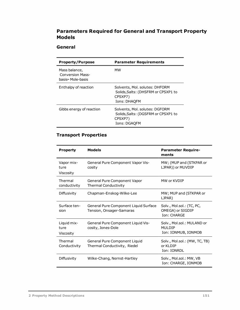
Parameters Required for General and Transport PropertyModels
General
Property/Purpose Parameter Requirements
Mass balance,Conversion Mass-basis↔Mole-basis
MW
Enthalpy of reaction Solvents, Mol. solutes: DHFORMSolids,Salts: (DHSFRM or CPSXP1 toCPSXP7)Ions: DHAQFM
Gibbs energy of reaction Solvents, Mol. solutes: DGFORMSolids,Salts: (DGSFRM or CPSXP1 toCPSXP7)Ions: DGAQFM
Transport Properties
Property Models Parameter Require-ments
Vapor mix-tureViscosity
General Pure Component Vapor Vis-cosity
MW; (MUP and (STKPAR orLJPAR)) or MUVDIP
Thermalconductivity
General Pure Component VaporThermal Conductivity
MW or KVDIP
Diffusivity Chapman-Enskog-Wilke-Lee MW;MUP and (STKPAR orLJPAR)
Surface ten-sion
General Pure Component Liquid SurfaceTension, Onsager-Samaras
Solv., Mol.sol.: (TC, PC,OMEGA) or SIGDIPIon: CHARGE
Liquidmix-tureViscosity
General Pure Component Liquid Vis-cosity, Jones-Dole
Solv., Mol.sol.: MULAND orMULDIPIon: IONMUB, IONMOB
ThermalConductivity
General Pure Component LiquidThermal Conductivity, Riedel
Solv., Mol.sol.: (MW, TC, TB)or KLDIPIon: IONRDL
Diffusivity Wilke-Chang, Nernst-Hartley Solv., Mol.sol.: MW, VBIon: CHARGE, IONMOB
2 Property Method Descriptions 151

Note: For surface tension and liquidmixture properties, the secondmethod is used onlyfor rigorous electrolyte properties.
Solids Handling PropertyMethodThe SOLIDS property method is designed for many kinds of solids processing:
l Coal processingl Pyrometallurgical processesl Miscellaneous other solids processing (such as starch and polymers)
The properties of solids and fluid phases cannot be calculated with the sametype of models. Therefore the components are distributed over the substreamsof types MIXED, CISOLID and NC and their properties are calculated with appro-priate models.
During the mechanical processing of raw materials (ore, coal, wood), physicalproperties can often be handled as nonconventional components with an overalldensity and an overall heat capacity. The characterization of nonconventionalcomponents and the specification of property models is discussed in the Defin-ing a Non-Conventional Component in the help. Details on nonconventional prop-erty methods are given in Nonconventional Component Enthalpy Calculation inOverview of Aspen Physical Property Methods. Details on nonconventional prop-erty models are given in Physical Property Models.
When the solids are decomposed into individual components (for example, toselectively undergo chemical reactions), they normally occur in the CISOLIDsubstream. The property models for these components are pure componentproperty models of the polynomial type. The components are not in phase equi-librium with the fluid components. Some examples are coal dust in air, burningcarbon, and sand in water. It is also possible to place conventional solids in theMIXED substream.
In pyrometallurgical applications, a CISOLID component can be in simultaneousphase and chemical equilibrium. This can happen only in the RGIBBS model, anequilibrium reactor based on Gibbs energy minimization. Under other con-ditions, the CISOLID component can undergo reactions but not phase equi-librium. As another exception, homogeneous solid mixture phases can occur inthe same reactor. The nonideality of solid mixtures can be handled using activ-ity coefficient models. To distinguish a solid mixture from single CISOLID com-ponents, they are placed in the MIXED substream.
In pyrometallurgical applications, many phases can occur simultaneously.These phases may need to be treated with different activity coefficient models(use the SOLIDS property method). For details, see Getting StartedModelingProcesses with Solids.
152 2 Property Method Descriptions

Fluid components always occur in the MIXED substream. They are treated withthe same fluid phase models as discussed in IDEAL. If non-ideality in the liquidphase occurs, the ideal activity coefficient model can be replaced.
Permanent gases may be dissolved in the liquid. You can model them usingHenry's law, which is valid at low concentrations.
Hydrometallurgical applications cannot be handled by the SOLIDS propertymethod. Use an electrolyte property method.
The transport property models for the vapor phase are all well suited for idealgases. The transport property models for the liquid phase are empirical equa-tions for fitting of experimental data.
The following table lists the models used in the SOLIDS property method andtheir parameter requirements. For details on these models, see Physical Prop-erty Models.
Parameters Required for the SOLIDS Property Method
General
Property/Purpose Parameter Requirements
Mass balance,Conversion Mass-basis↔Mole-basis
MW
Conversion Stdvol-basis↔Mole-basis VLSTD
Free-water option: solubility of water inorganic phase
WATSOL
Enthalpy of reaction DHFORM, (DHSFRM or CPSXP1 toCPSXP7)
Gibbs energy of reaction DGFORM, (DGSFRM or CPSXP1 toCPSXP7)
Thermodynamic Properties
Property Models Parameter Require-ments
Vapor pure andmixtureFugacityCoefficient
Ideal gas law
2 Property Method Descriptions 153
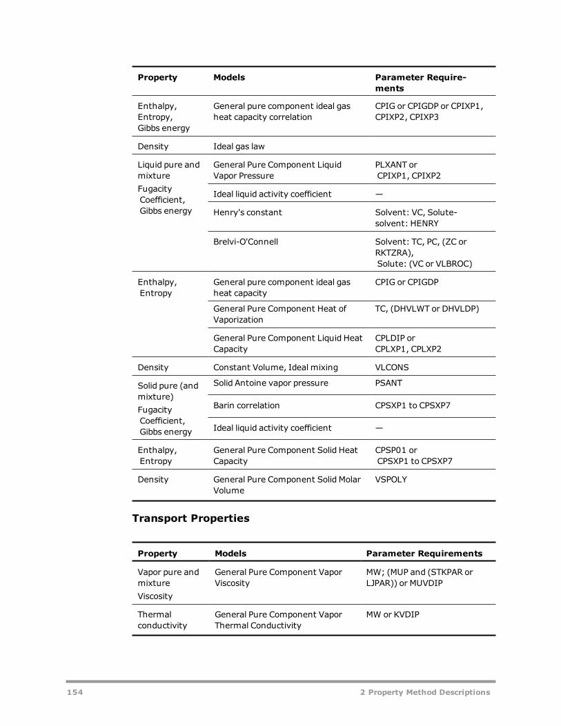
Property Models Parameter Require-ments
Enthalpy,Entropy,Gibbs energy
General pure component ideal gasheat capacity correlation
CPIG or CPIGDP or CPIXP1,CPIXP2, CPIXP3
Density Ideal gas law
Liquid pure andmixtureFugacityCoefficient,Gibbs energy
General Pure Component LiquidVapor Pressure
PLXANT orCPIXP1, CPIXP2
Ideal liquid activity coefficient —
Henry's constant Solvent: VC, Solute-solvent: HENRY
Brelvi-O'Connell Solvent: TC, PC, (ZC orRKTZRA),Solute: (VC or VLBROC)
Enthalpy,Entropy
General pure component ideal gasheat capacity
CPIG or CPIGDP
General Pure Component Heat ofVaporization
TC, (DHVLWT or DHVLDP)
General Pure Component Liquid HeatCapacity
CPLDIP orCPLXP1, CPLXP2
Density Constant Volume, Ideal mixing VLCONS
Solid pure (andmixture)FugacityCoefficient,Gibbs energy
Solid Antoine vapor pressure PSANT
Barin correlation CPSXP1 to CPSXP7
Ideal liquid activity coefficient —
Enthalpy,Entropy
General Pure Component Solid HeatCapacity
CPSP01 orCPSXP1 to CPSXP7
Density General Pure Component Solid MolarVolume
VSPOLY
Transport Properties
Property Models Parameter Requirements
Vapor pure andmixtureViscosity
General Pure Component VaporViscosity
MW; (MUP and (STKPAR orLJPAR)) or MUVDIP
Thermalconductivity
General Pure Component VaporThermal Conductivity
MW or KVDIP
154 2 Property Method Descriptions

Property Models Parameter Requirements
Diffusivity Chapman-Enskog-Wilke-Lee MW;MUP and (STKPAR orLJPAR)
Surface tension General Pure Component LiquidSurface Tension
(TC, PC, OMEGA) orSIGDIP
Liquid pure andmixtureViscosity
General Pure Component LiquidViscosity
MULAND or MULDIP
ThermalConductivity
General Pure Component LiquidThermal Conductivity
(MW, TC, TB) or KLDIP
Diffusivity Wilke-Chang MW, VB
Solids pureThermalConductivity
Solids polynomial KSPOLY
Steam TablesThe following table lists the names of the steam table property methods avail-able in Aspen Physical Property System.
Steam tables can calculate all thermodynamic properties for systems con-taining pure water or steam. For mixtures of water and other components,refer to the beginning of this chapter for more help.
For process calculations, the accuracy of all three models is adequate. TheSTEAM-TA method is made up of different correlations covering differentregions of the P-T space. These correlations do not provide continuity at theboundaries, which can lead to convergence problems and predict wrong trends.STMNBS2 can also have this problem. STEAMNBS does not have this problemand it extrapolates better, so it may be a better choice when there are not otherconsiderations. For similar reasons, it may be better to use STEAMNBS withproperty methods such as SRK that calculate water properties from the free-water property method.
The transport property models for both property methods are from the Inter-national Association for Properties of Steam (IAPS).
All models have built-in parameters. For details, see ASME Steam Tables,NBS/NRC Steam Tables, and IAPWS-95 Steam Tables in Physical PropertyModels.
2 Property Method Descriptions 155
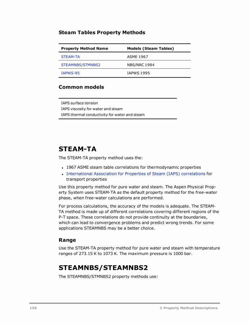
Steam Tables Property Methods
Property Method Name Models (Steam Tables)
STEAM-TA ASME 1967
STEAMNBS/STMNBS2 NBS/NRC 1984
IAPWS-95 IAPWS 1995
Common models
IAPS surface tensionIAPS viscosity for water and steamIAPS thermal conductivity for water and steam
STEAM-TAThe STEAM-TA property method uses the:
l 1967 ASME steam table correlations for thermodynamic propertiesl International Association for Properties of Steam (IAPS) correlations fortransport properties
Use this property method for pure water and steam. The Aspen Physical Prop-erty System uses STEAM-TA as the default property method for the free-waterphase, when free-water calculations are performed.
For process calculations, the accuracy of the models is adequate. The STEAM-TA method is made up of different correlations covering different regions of theP-T space. These correlations do not provide continuity at the boundaries,which can lead to convergence problems and predict wrong trends. For someapplications STEAMNBS may be a better choice.
RangeUse the STEAM-TA property method for pure water and steam with temperatureranges of 273.15 K to 1073 K. The maximum pressure is 1000 bar.
STEAMNBS/STEAMNBS2The STEAMNBS/STMNBS2 property methods use:
156 2 Property Method Descriptions

l 1984 NBS/NRC steam table correlations for thermodynamic propertiesl International Association for Properties of Steam (IAPS) correlations fortransport properties
The STMNBS2 uses the same equations as STEAMNBS but with a different rootsearch method.
Use these property methods for pure water and steam, and in particular for thefree-water phase.
RangeUse the STEAMNBS/STMNBS2 property methods for pure water and steam withtemperature ranges of 273.15 K to 2000 K. The maximum pressure is over10000 bar. The STEAMNBS method is recommended for use with the SRK,BWRS, MXBONNEL and GRAYSON2 property methods.
IAPWS-95 Property MethodThe IAPWS-95 property method uses the
l 1995 IAPWS steam table correlations for thermodynamic properties
Use this property method for pure water and steam, in particular for the free-water phase.
IAPWS-95 is the current standard steam table from the International Asso-ciation for the Properties of Water and Steam. It replaces the previous 1984 for-mulation (IAPS-84) implemented in Aspen Plus as STEAMNBS and STMNBS2.IAPWS-95 overcomes several shortcomings of IAPS-84, including weaknessesnear the critical point (regarding the phase boundary and in its derivative prop-erties such as isothermal compressibility) and when extrapolating beyond itsrange of validity.
The IAPWS-95 formulation is in the form of a fundamental equation explicit inHelmholtz free energy. The residual part of the Helmholtz free energy was fit-ted to the following properties: (a) thermal properties of the single-phaseregion (pρT) and of the vapor-liquid phase boundary (pρ’ρ”T), including thephase-equilibrium conditions (Maxwell criterion), and (b) the caloric properties- specific isochoric heat capacity, specific isobaric heat capacity, speed ofsound, differences in the specific enthalpy and in the specific internal energy,Joule-Thomson coefficient, and isothermal throttling coefficient.
Region & Property Estimated Uncertainty
Liquid – density ±0.001% to ±0.02%
Liquid – speed of sound ±0.03% to ±0.2%
Liquid – isobaric heat capacity ±0.1%
2 Property Method Descriptions 157

Liquid at ambient pressure – density ≤0.0001%
Liquid at ambient pressure – speed of sound ±0.005%
Gas – density ±0.03% to ±0.05%
Gas – speed of sound ±0.15%
Gas – isobaric heat capacity ±0.2%
RangeThe IAPWS-95 formation covers a validity range for temperatures from themelting line (lowest temperature 251.2 K at 209.9 MPa) to 1273 K and pres-sures up to 1000 MPa. In this entire range of validity, it represents even themost accurate data to within their experimental uncertainty.
In the stable fluid region, the IAPWS-95 formulation can be extrapolated bey-ond the limits of validity listed above. The model behaves reasonably wellwhen extrapolated to pressures up to 2000 MPa and temperatures up to 3000 Kas long as the conditions are in the fluid region (less than melting pressure atspecified temperature, and greater than melting temperature at specified pres-sure).
158 2 Property Method Descriptions

3 Property Calculation Meth-ods and Routes
In the Aspen Physical Property System the methods and models used to cal-culate thermodynamic and transport properties are packaged in property meth-ods. Each property method contains all the methods and models needed for acalculation. A unique combination of methods and models for calculating a prop-erty is called a route.
Physical Property Methods in Using the Property Environment in the helpdescribes the property methods available in the Aspen Physical Property Sys-tem, provides guidelines for choosing an appropriate property method for yourcalculation, and describes how to modify property methods to suit your cal-culation needs by replacing property models.
This chapter discusses:
l Major, subordinate, and intermediate properties in the Aspen PhysicalProperty System
l Calculation methods availablel Routing conceptsl Property models availablel Tracing routesl Modifying and creating property methodsl Modifying and creating routes
IntroductionMost properties are calculated in several steps. An example is the calculation ofthe fugacity coefficient of a component in a liquid mixture:
ϕ γ ϕ= *il
i il, (1)
Where:
3 Property Calculation Methods and Routes 159

ϕ*il, = ϕ p
p
* *iviv, , (2)
Equations 1 and 2 are both derived from thermodynamics. The equations relatethe properties of interest (φi
l,φi*,l)to other properties (γi, φi
*,v, pi*,l) and state
variables (xi, p). In general, this type of equation is derived from universal sci-entific principles. These equations are calledmethods.
In the computation of the liquid mixture fugacity, you need to calculate:
l Activity coefficient (γi)l Vapor pressure (pi
*,l)l Pure component vapor fugacity coefficient
This type of property is usually calculated using equations that depend on uni-versal parameters like Tcand pc; state variables, such as T and p; and cor-relation parameters. The use of correlation parameters makes these equationsmuch less universal and more subjective than methods. For distinction, we callthem models. Often several models exist to calculate one property. Forexample, to calculate γi you can use the NRTL, UNIQUAC, or UNIFAC model.
The reason for treating models and methods separately is to allow for max-imum flexibility in property calculations. Therefore the descriptions providedshould help show the flexibility of the Aspen Physical Property System, ratherthan constitute definitions. For detailed descriptions and lists of available meth-ods and models, see Methods and Routes and Models.
A complete calculation route consists of a combination of methods and models.A number of frequently used routes have been defined in the Aspen PhysicalProperty System. Routes that belong logically together have been grouped toform property methods. For more about property methods, see PropertyMethod Descriptions. Routes are discussed in detail in Routes and Models.
To choose a different calculation route for a given property route than what isdefined in a property method, you can exchange routes or models in propertymethods (See Modifying and Creating Property Methods).
For a specific property, there are many choices of models and methods used tobuild a route. Therefore the Aspen Physical Property System does not containall possible routes as predefined routes. However you can freely construct cal-culation routes according to your needs. This is a unique feature of the AspenPhysical Property System. Modifying and creating new routes from existingmethods, routes and models, and using them in modified or new property meth-ods is explained in Modifying and Creating Routes.
160 3 Property Calculation Methods and Routes
Physical Properties in theAspen Physical Property Sys-temThe following properties may be required by Aspen Physical Property Systemcalculations:
l Thermodynamic Propertiesl Fugacity coefficients (for K values)l Enthalpyl Entropyl Gibbs energyl Molar volumel Transport Propertiesl Viscosityl Thermal conductivityl Diffusion coefficientl Surface tension
The properties required by unit operation models in the Aspen Physical PropertySystem are calledmajor properties and are listed in the table labeled MajorProperties in the Aspen Physical Property System. A major property maydepend on other major properties. In addition, a major property may dependon other properties that are not major properties. These other properties canbe divided into two categories: subordinate properties and intermediate prop-erties.
Subordinate properties may depend on other major, subordinate or inter-mediate properties, but are not directly required for unit operation model cal-culations. Examples of subordinate properties are enthalpy departure andexcess enthalpy. The table labeled Subordinate Properties in the Aspen PhysicalProperty System lists the subordinate properties.
Intermediate properties are calculated directly by property models, rather thanas fundamental combinations of other properties. Common examples of inter-mediate properties are vapor pressure (calculated by performing a bubble pointflash) and activity coefficients. The table labeled Intermediate Properties in theAspen Physical Property System lists the intermediate properties.
Major and subordinate properties are obtained by a method evaluation. Inter-mediate properties are obtained by a model evaluation.
3 Property Calculation Methods and Routes 161

Major Properties in the Aspen Physical Prop-erty System
PropertyName
Symbol Description
PHIV φi*,v Vapor pure component fugacity coefficient
PHIL φi*,l Liquid pure component fugacity coefficient
PHIS φi*,s Solid pure component fugacity coefficient
PHIVMX φiv Vapor fugacity coefficient of a component in a mixture
PHILMX φil Liquid fugacity coefficient of a component in a mixture
PHISMX φis Solid fugacity coefficient of a component in a mixture
HV Hi*,v Vapor pure component molar enthalpy
HL Hi*,l Liquid pure component molar enthalpy
HS Hi*,s Solid pure component molar enthalpy
HVMX Hmv Vapor mixture molar enthalpy
HLMX Hml Liquidmixture molar enthalpy
HSMX Hms Solidmixture molar enthalpy
GV μi*,v Vapor pure component molar Gibbs free energy
GL μi*,l Liquid pure component molar Gibbs free energy
GS μi*,s Solid pure component molar Gibbs free energy
GVMX Gmv Vapor mixture molar Gibbs free energy
GLMX Gml Liquidmixture molar Gibbs free energy
GSMX Gms Solidmixture molar Gibbs free energy
SV Si*,v Vapor pure component molar entropy
SL Si*,l Liquid pure component molar entropy
SS Si*,s Solid pure component molar entropy
SVMX Smv Vapor mixture molar entropy
SLMX Sml Liquidmixture molar entropy
SSMX Sms Solidmixture molar entropy
VV Vi*,v Vapor pure component molar volume
VL Vi*,l Liquid pure component molar volume
162 3 Property Calculation Methods and Routes

PropertyName
Symbol Description
VS Vi*,s Solid pure component molar volume
VVMX Vmv Vapor mixture molar volume
VLMX Vml Liquidmixture molar volume
VSMX Vms Solidmixture molar volume
MUV ηi*,v Vapor pure component viscosity
MUL ηi*,l Liquid pure component viscosity
MUVMX ηv Vapor mixture viscosity
MULMX ηl Liquidmixture viscosity
KV λi*,v Vapor pure component thermal conductivity
KL λi*,l Liquid pure component thermal conductivity
KS λi*,s Solid pure component thermal conductivity
KVMX λv Vapor mixture thermal conductivity
KLMX λl Liquidmixture thermal conductivity
KSMX λs Solidmixture thermal conductivity
DV Dijv Vapor binary diffusion coefficient
DL Dijl Liquid binary diffusion coefficient
DVMX Div Vapor diffusion coefficient of a component in a mixture
DLMX Dil Liquid diffusion coefficient of a component in a mixture
at infinite dilution
SIGL σi*,l Pure component surface tension
SIGLMX σl Mixture surface tension
Subordinate Properties in the Aspen Phys-ical Property System
PropertyName
Symbol Description
DHV Hi*,v-
Hi*,ig
Vapor pure component molar enthalpy departure
DHL Hi*,l -
Hi*,ig
Liquid pure component molar enthalpy departure
3 Property Calculation Methods and Routes 163

PropertyName
Symbol Description
DHS Hi*,s -
Hi*,ig
Solid pure component molar enthalpy departure
DHVMX Hmv- Hm
ig Vapor mixture molar enthalpy departure
DHLMX Hml - Hm
ig Liquidmixture molar enthalpy departure
DHSMX Hms- Hm
ig Solidmixture molar enthalpy departure
DHVPC Hi*,v(p) -
Hi*,v(pi
*)Vapor pure component molar enthalpy departure pres-sure correction
DHLPC Hi*,l(p) -
Hi*,s(pi
*)Liquid pure component molar enthalpy departure pres-sure correction
DHSPC Hi*,l(p) -
Hi*,s(pi
*)Solid pure component molar enthalpy departure pres-sure correction
DGV μi*,v -
μi*,ig
Vapor pure component molar Gibbs energy departure
DGL μi*,l-μi
*,ig Liquid pure component molar Gibbs energy departure
DGS μi*,s-μi
*,ig Solid pure component molar Gibbs energy departure
DGVMX Gmv - Gm
ig Vapor mixture molar Gibbs energy departure
DGLMX Gml- Gm
ig Liquidmixture molar Gibbs energy departure
DGSMX Gms- Gm
ig Solidmixture molar Gibbs energy departure
DGVPC μi*,v(p) -
μi*,v(pi
*)Vapor pure component molar Gibbs energy departurepressure correction
DGLPC μi*,l(p) -
μi*,l(pi
*)Liquid pure component molar Gibbs energy departurepressure correction
DGSPC μi*,s(p) -
μi*,s(pi
*)Solid pure component molar Gibbs energy departurepressure correction
DSV Si*,v -
Si*,ig
Vapor pure component molar entropy departure
DSL Si*,l- Si
*,ig Liquid pure component molar entropy departure
DSS Si*,s- Si
*,ig Solid pure component molar entropy departure
DSVMX Smv- Sm
ig Vapor mixture molar entropy departure
DSLMX Sml- Sm
ig Liquidmixture molar entropy departure
DSSMX Sms- Sm
ig Solidmixture molar entropy departure
164 3 Property Calculation Methods and Routes
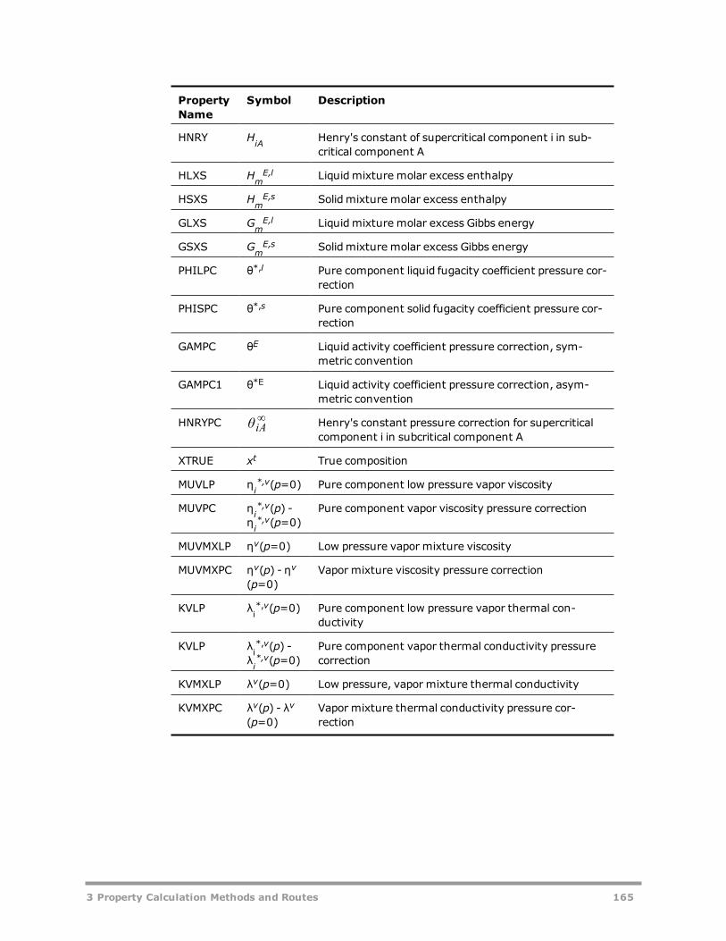
PropertyName
Symbol Description
HNRY HiA Henry's constant of supercritical component i in sub-critical component A
HLXS HmE,l Liquidmixture molar excess enthalpy
HSXS HmE,s Solidmixture molar excess enthalpy
GLXS GmE,l Liquidmixture molar excess Gibbs energy
GSXS GmE,s Solidmixture molar excess Gibbs energy
PHILPC θ*,l Pure component liquid fugacity coefficient pressure cor-rection
PHISPC θ*,s Pure component solid fugacity coefficient pressure cor-rection
GAMPC θE Liquid activity coefficient pressure correction, sym-metric convention
GAMPC1 θ*E Liquid activity coefficient pressure correction, asym-metric convention
HNRYPC θiA∞ Henry's constant pressure correction for supercritical
component i in subcritical component A
XTRUE xt True composition
MUVLP ηi*,v(p=0) Pure component low pressure vapor viscosity
MUVPC ηi*,v(p) -
ηi*,v(p=0)
Pure component vapor viscosity pressure correction
MUVMXLP ηv(p=0) Low pressure vapor mixture viscosity
MUVMXPC ηv(p) - ηv(p=0)
Vapor mixture viscosity pressure correction
KVLP λi*,v(p=0) Pure component low pressure vapor thermal con-
ductivity
KVLP λi*,v(p) -
λi*,v(p=0)
Pure component vapor thermal conductivity pressurecorrection
KVMXLP λv(p=0) Low pressure, vapor mixture thermal conductivity
KVMXPC λv(p) - λv(p=0)
Vapor mixture thermal conductivity pressure cor-rection
3 Property Calculation Methods and Routes 165

Intermediate Properties in the Aspen Phys-ical Property System
PropertyName
Symbol Description
GAMMA γ Liquid phase activity coefficient
GAMUS γ* Liquid phase activity coefficient, unsymmetric con-vention
GAMMAS γs Solid phase activity coefficient
WHNRY w Henry's constant mixing rule weighting factor
PL pi*,l Liquid pure component vapor pressure
PS pi*,s Solid pure component vapor pressure
DHVL ΔvapHi* Pure component enthalpy of vaporization
DHLS ΔfusHi* Pure component enthalpy of fusion
DHVS ΔsubHi* Pure component enthalpy of sublimation
VLPM Vil Partial molar liquid volume
MethodsThis section describes the methods available for calculating the major and sub-ordinate properties in the Aspen Physical Property System.
A method is an equation used to calculate physical properties based on uni-versal scientific principles only, such as thermodynamics. This equation maycontain assumptions, such as the vapor can be treated as ideal gas or the pres-sure is low enough to neglect the pressure correction. The equation may needproperties and state variables but not correlation parameters to calculate a spe-cific property.
Applied thermodynamics indicate that there usually is more than one methodfor calculating a particular property. For example, the enthalpy departure of acomponent in the liquid phase, Hi
*,l- Hi*,ig can be calculated from its fugacity
coefficient in the liquid phase:
H H RTφ
T* − * = −
∂ln *
∂il
iig i
l, , 2
,
166 3 Property Calculation Methods and Routes

This method is often used for supercritical solutes in liquid solution. Altern-atively, the liquid departure function can be calculated from the vapor enthalpydeparture and the heat of vaporization:
H H H H H* − * = * − * − ∆il
iig
iν
iig
vap i, , , ,
Both methods are equally valid. There is another possibility, which is to cal-culate the departure function directly by an equation of state. Equations of stateuse correlation parameters and are therefore classified as models, so:
H H f p T* − * = ( , , correlationparameters)il
iig, ,
This is not a method but rather a valid alternative to calculate the enthalpydeparture. To make the model available to the list of methods, a simple methodis used that refers to a model:
H H f p T* − * = ( , , specified model)il
iig, ,
In general, a list of methods available for a property will be similar to the listpresented here for the enthalpy departure. Compare these tables:
Vapor Fugacity Coefficient Methods Vapor Entropy Methods
Liquid Fugacity Coefficient Methods Liquid Entropy Methods
Solid Fugacity Coefficient Methods Solid Entropy Methods
Vapor Enthalpy Methods Molar Volume Methods
Liquid Enthalpy Methods Viscosity Methods
Solid Enthalpy Methods Thermal Conductivity Methods
Vapor Gibbs Energy Methods Diffusion Coefficient Methods
Liquid Gibbs Energy Methods Surface Tension Methods
Solid Gibbs Energy Methods
In a method you can have any number of major properties, subordinate prop-erties, or models. Usually there is a method that can be used with an equationof state approach and an alternative that is used with the activity coefficientapproach (see Thermodynamic Property Methods in Overview of Aspen PhysicalProperty Methods). There is always a method that refers to a model. Althoughthere are a limited number of thermodynamic methods, in general, all the exist-ing thermodynamic methods for each property are present.
Transport property methods are not as universal as thermodynamic methods.Therefore the transport property methods offered in the Aspen Physical Prop-erty System might not be exhaustive, but multiple methods for one propertyalso exist.
3 Property Calculation Methods and Routes 167
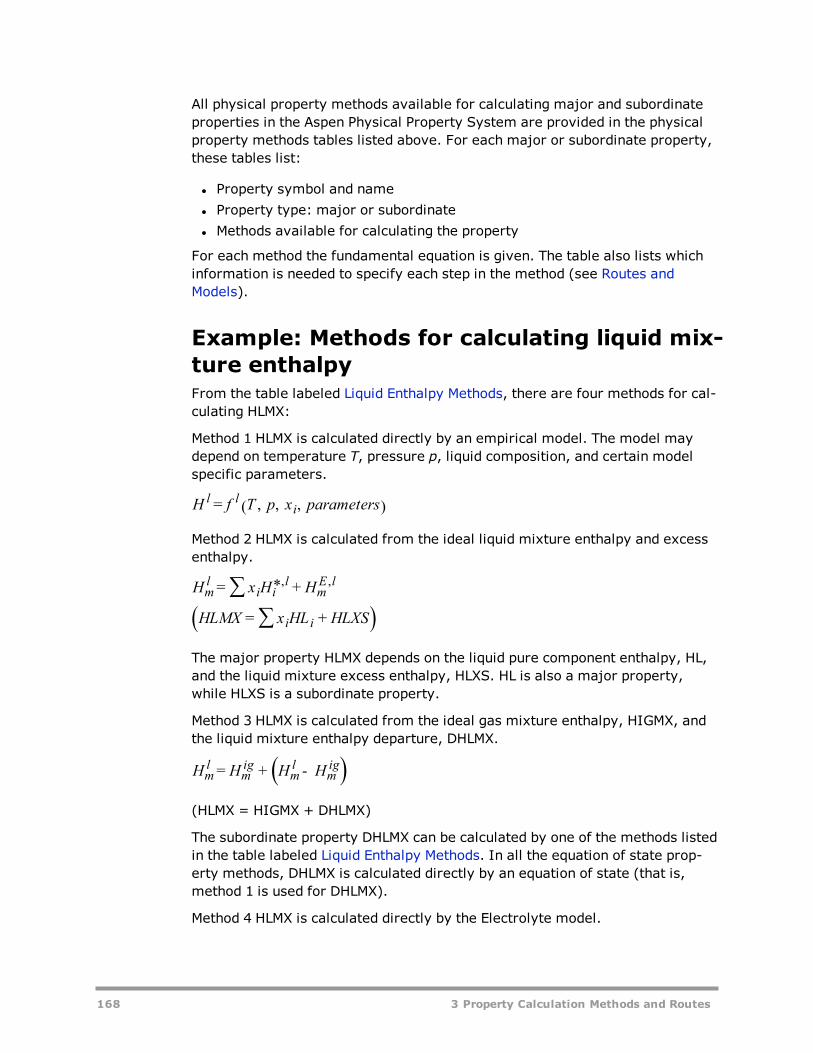
All physical property methods available for calculating major and subordinateproperties in the Aspen Physical Property System are provided in the physicalproperty methods tables listed above. For each major or subordinate property,these tables list:
l Property symbol and namel Property type: major or subordinatel Methods available for calculating the property
For each method the fundamental equation is given. The table also lists whichinformation is needed to specify each step in the method (see Routes andModels).
Example: Methods for calculating liquid mix-ture enthalpyFrom the table labeled Liquid Enthalpy Methods, there are four methods for cal-culating HLMX:
Method 1 HLMX is calculated directly by an empirical model. The model maydepend on temperature T, pressure p, liquid composition, and certain modelspecific parameters.
H f T p x parameters= ( , , , )l l
i
Method 2 HLMX is calculated from the ideal liquid mixture enthalpy and excessenthalpy.
( )
∑
∑
H x H H
HLMX x HL HLXS
= * +
= +
ml
i il
mE l
i i
, ,
The major property HLMX depends on the liquid pure component enthalpy, HL,and the liquid mixture excess enthalpy, HLXS. HL is also a major property,while HLXS is a subordinate property.
Method 3 HLMX is calculated from the ideal gas mixture enthalpy, HIGMX, andthe liquid mixture enthalpy departure, DHLMX.
( )H H H H= + −ml
mig
ml
mig
(HLMX = HIGMX + DHLMX)
The subordinate property DHLMX can be calculated by one of the methods listedin the table labeled Liquid Enthalpy Methods. In all the equation of state prop-erty methods, DHLMX is calculated directly by an equation of state (that is,method 1 is used for DHLMX).
Method 4 HLMX is calculated directly by the Electrolyte model.
168 3 Property Calculation Methods and Routes

H f x= ( )ml t
Where:
xt = The component true mole fractions
(xt is also the symbol for the subordinate property XTRUE:HLMX = f (XTRUE)).
Vapor Fugacity Coefficient Methods
Property Sym-boland Name
PropertyType
MethodCode
Method Route Structure InformationRequired
φi*,v
PHIVMajor 1 Specified
modelφi*,v Model name
φiv
PHIVMXMajor 1 Specified
modelφiv Model name (Default: φi
v=1)
2 φiv=f(yi,
φi*,v)
φi*,v Route ID
φiv Model name
3 φiv=f(γi) γi Model name
φiv Model name
Liquid Fugacity Coefficient Methods
PropertySymbolandName
PropertyType
MethodCode Method
Route StructureInformationRequired
φi*,l
PHILMajor 1 Specifiedmodel φi
*,l Model name
2 ( )φ T p p θ
p
* , * * *iv
ililil, , , , p*,l Model name
φi*,v Model name
(Default: φi*,v = 1)
θ*,l Route ID(Default: θ*,l = 1)
3 Property Calculation Methods and Routes 169

PropertySymbolandName
PropertyType
MethodCode Method
Route StructureInformationRequired
3 Specifiedmodel for supercritical com-ponents
For subcritical components:
( ) ∫φ T pp
p RTV dp* , *
*exp
1*
iv
il i
l
p
p l, ,,
*,
il,
φi*,l Model name
p*,l Model nameφi*,l Model name
Vi*,l Model Name
4 Steam table for water, otherwise from
( )φ T p p θ
p
* , * * *iv
ililil, , , ,
p*,l Model nameφi*,v Model name
(Default: φi*,v = 1)
θ*,l Route ID(Default: θ*,l = 1)
θi*,l
PHILPCSubord. 1
∫RTV dpexp
1*
p
p l
*,
il,
p*,l Model nameVi*,lModel Name
2 Specifiedmodel θi*,l Model name
φil
PHILMXMajor 1 Specifiedmodel φi
lModel name
2 γiφi*,lθi
E γi Model name(Default: γi = 1)φi*,l Route ID
θiERoute ID
(Default: θiE = 1)
3 Unsymmetric Convention
For subcritical components (A or B): φA*,l Route ID
φAl=δAγAφA
*,l γAModel name(Default: γA= 1)
For supercritical components (i or j)
φ γH
pγ=il
ii
i∞
Where:
170 3 Property Calculation Methods and Routes

PropertySymbolandName
PropertyType
MethodCode Method
Route StructureInformationRequired
∑δw
xx
H
γ
H
γln = ln − lnA
A
A j
jiA
jA
j
j∞ ∞
(or δA= 1)
HjA Route IDwAModel option code
∑H
γw
H
γln = lni
i B
BiB
iB∞ ∞
wBModel namewBModel option code
( )∑
γ γln = lim lni
xi
∞
→0j j
∑ w = 1
B
BMethod Option code†0: Do not calculateHi1: Calculate Hi(Default = 0 )
4 γ φ θ*i i
liE, γi Model name
(Default: γi = 1)φi*,l Route ID
θiE Route ID
(Default: θiE = 1)
Where:
γi = f(xt) (Default: θi
E = 1)xt Route ID
5 Unsymmetric Convention
For subcritical components (A or B): φi*,l Route ID
φ δ γ φ= *Al
A A Al, γAModel name
(Default: γA= 1)
Where:
γ f x= ( )At xt Route ID
3 Property Calculation Methods and Routes 171

PropertySymbolandName
PropertyType
MethodCode Method
Route StructureInformationRequired
For supercritical components (i or j)
φ γH
pγ=il
ii
i∞
Where:
∑δW
Xx
H
γ
H
γln = ln − lnA
A
A j
jiA
jA
j
j∞ ∞
(or δA= 1)
HjA Route IDwAModel option code
∑H
γw
H
γln = lni
i B
BiB
iB∞ ∞
wBModel namewBModel option code
( )∑
γ γln = lim lni
xi
∞
→0j j
∑ w = 1
B
BMethod Option code†0: Do not calculateHi1: Calculate Hi(Default = 0 )
6 φil = f(γi) γi Model name
φil Model name
7 Similar to method 3, but the fugacity coefficients of some com-ponents can be overridden by a special PHILMXmodel. Currently,this method is used to override the fugacity coefficients of CO2,H2S, NH3, and H2O calculated by an activity coefficient propertymethod by the API sour water model.
xt
XTRUESubord. 1 ( )x f T x γ= , , , Chemistryt
i iγi Model name
θiE
GAMPCSubord. 1
( )∫RTV V dpexp
1− *
p
p
il
il,
ref
Vil Model name
Vi*,lModel name
2 Specifiedmodel θiE Model name
172 3 Property Calculation Methods and Routes

PropertySymbolandName
PropertyType
MethodCode Method
Route StructureInformationRequired
θi*,E
GAMPC1Subord. 1
∫RTV dpexp
1
p
p
il
ref
Vil Model name
2 Specifiedmodel θi*,E Model name
HiAHNRY
Subord. 1 Specifiedmodel HiAModel name
2 ( )H p T θ,iAref
iA∞ HiAModel name
θiA∞ Route ID
(Default: θiA∞ = 1)
pref defined by thepref option code ofHNRYPC
θiA∞
HNRYPC
Subord. 1
∫RTV dpexp
1
p
p
il
ref
pA*,l Model name (if
needed for pref
V i∞Model name
2 Specifiedmodel θiA∞ Model name
† For calculating fugacity coefficients, Hi is not needed explicitly; the quantity
needed is H γ/i i∞
. Methods which can calculate this quantity directly have anoption code to force the calculation of Hi. This can be set to 1 when Hi is neededfor Property Set property reporting. Certain property methods need Hi for otherreasons and these methods set this option code to 1.
Solid Fugacity Coefficient Methods
Property Symbol andName
PropertyType
MethodCode Method
Route StructureInformationRequired
φi*,s
PHISMajor 1 Specified Model φi
*,s Model name
3 Property Calculation Methods and Routes 173

Property Symbol andName
PropertyType
MethodCode Method
Route StructureInformationRequired
2( )φ T p p
θ
p* , * *
*
iv
isis i
s, , ,
, pi*,s Model name
φi*,v Model name
(Default: φi*,v = 1)
θi*,s Route ID
(Default: θi*,s = 1)
3 φi*,sφi
*,l φi*,s Model name
φi*,l Route ID
θi*,s
PHISPCSubord. 1
∫RTV dpexp
1*
p
p
is
*
,
s,
pi*,s Model name
Vi*,s Model name
2 Specifiedmodel θi*,s Model name
φis
PHISMXMajor 1 Specifiedmodel φi
s Model name
2 φis = f(xi
s, φi*,s) φi
*,s Route IDφis Model name
3 γisφi
*,s γis Model name
φi*,s Route ID
Vapor Enthalpy Methods
Property Sym-bol and Name
PropertyType
MethodCode Method
Route StructureInformation Required
Hi*,v
HVMajor 1 Specifiedmodel Hi
*,v Model name
2 ( )H H H* + * − *iig
iν
iig, , , (Hi
*,v -Hi*,ig) Route ID
(Default:Hi*,v -Hi
*,ig=0)
3 Hi*,l + ΔvapHi
* Hi*,l Route ID
ΔvapHi* Model name
Hi*,v -Hi
*,ig
DHVSubord. 1 Specifiedmodel (Hi
*,v -Hi*,ig) Model name
2RT
φ
T−
∂ln *
∂
iv
2,
φi*,v Model name
174 3 Property Calculation Methods and Routes

Property Sym-bol and Name
PropertyType
MethodCode Method
Route StructureInformation Required
Hmv
HVMXMajor 1 Specifiedmodel Hm
v Model name
2 ∑ y H*ii i
ν, Hi*,v Route ID
3 Hmig + (Hm
v -Hmig) (Hm
v -Hmig) Route ID
(Default:Hmv -Hm
ig=0)
4 Specifiedmodel Hi*,v Hi
*,v Route IDHm
v Model name used toprovide mixing rules forthe pure component prop-erty Hi
*,v
Hmv -Hm
ig
DHVMXSubord. 1 Specifiedmodel (Hm
v -Hmig) Model name
2∑RT y
φ
T−
∂ln
∂ii
iv
2
φiv Model name
3 Hmv -Hm
ig = f(γi) γi Model nameEquation of state modelname
Liquid Enthalpy Methods
PropertySymboland Name
PropertyType
MethodCode Method
Route StructureInformation Required
Hi*,l
HLMajor 1 Specifiedmodel Hi
*,l Model name
2 Hi*,ig + (Hi
*,l -Hi*,ig) (Hi
*,l -Hi*,ig) Route ID
Hi*,l -Hi
*,ig
DHLSubord. 1 Specifiedmodel (Hi
*,l -Hi*,ig) Model name
2RT
φ
T−
∂ln *
∂
il
2,
φi*,l Model name
3 Property Calculation Methods and Routes 175

PropertySymboland Name
PropertyType
MethodCode Method
Route StructureInformation Required
3 (Hi*,v(T, pi
*,l) -Hi*,ig(T))
- ΔvapHi*(T)
+ (Hi*,l(T, p) -Hi
*,l(T, pi*,l))
pil Model name
(Hi*,v -Hi
*,ig) Route ID(Default:Hi
*,v -Hi*,ig = 0)
ΔvapHil Model name
(Hi*,l(T, p) -Hi
*,l(T, pi*,l))
Route ID(Default: (Hi
*,l(T, p) -Hi*,l
(T, pi*,l)) = 0)
4 (Hi*,v(T, pi
*,l) -Hi*,ig(T))
- ΔvapHi*(T)
+ (Hi*,l(T, p) -Hi
*,l(T, pi*,l))
for polymer property method
pil Model name
(Hi*,v -Hi
*,ig) Route ID(Default:Hi
*,v -Hi*,ig = 0)
ΔvapHil Model name
(Hi*,l(T, p) -Hi
*,l(T, pi*,l))
Route ID(Default: (Hi
*,l(T, p) -Hi*,l
(T, pi*,l)) = 0)
5 (Hi*,v(T, pi
*,l) -Hi*,ig(T))
- ΔvapHi*(T)
+ (Hi*,l(T, p) -Hi
*,l(T, pi*,l))
for electrolyte activity coefficientproperty method
pil Model name
(Hi*,v -Hi
*,ig) Route ID(Default:Hi
*,v -Hi*,ig = 0)
ΔvapHil Model name
(Hi*,l(T, p) -Hi
*,l(T, pi*,l))
Route ID(Default: (Hi
*,l(T, p) -Hi*,l
(T, pi*,l)) = 0)
(Hi*,l(T, p) -
Hi*,l(T,
pi*,l))
DHLPC
Subord. 1 (Hi*,l(T, p) -Hi
*,ig(T)) -(Hi
*,l(T, pi*,l) -Hi
*,ig(T))pi*,l Model name
(Hi*,l -Hi
*,ig) Route ID
2
∫ V TV
Tdp* −
∂ *
∂p
p
il i
l
p
,,
i
pi*,l Model name
Vi*,l Model name
Integration option code(Default: 1 point )
3 Specifiedmodel ()( )
H T p
H T p
* ( , ) −
* , *
il
il
il
,
, ,
Model
name
176 3 Property Calculation Methods and Routes

PropertySymboland Name
PropertyType
MethodCode Method
Route StructureInformation Required
Hml
HLMXMajor 1 Specifiedmodel Hm
l Model name
2 ∑ x H H* +
i
i il
mE l, , Hi
*,l Route IDHiE,l Route ID
(Default:HiE,l =0)
3 Hmig + (Hm
l -Hmig) (Hm
l -Hmig) Route ID
4 Electrolyte model (xt) Hml Model name
xt Route ID
5 Specifiedmodel Hi*,l Hi
*,l Route IDHm
l Model name used toprovide mixing rules forthe pure component prop-erty Hi
*,l
6 Hmig + (Hm
l -Hmig) for electrolyte
system(Hm
l -Hmig) Route ID
Hml -Hm
ig
DHLMXSubord. 1 Specifiedmodel (Hm
l -Hmig) Model name
2 ( )∑ x H H H* − * +
i
i il
iig
mE l, , , (Hi
*,l -Hi*,ig) Route ID
HmE,l Route ID
(Default:HmE,l = 0)
3 Property Calculation Methods and Routes 177
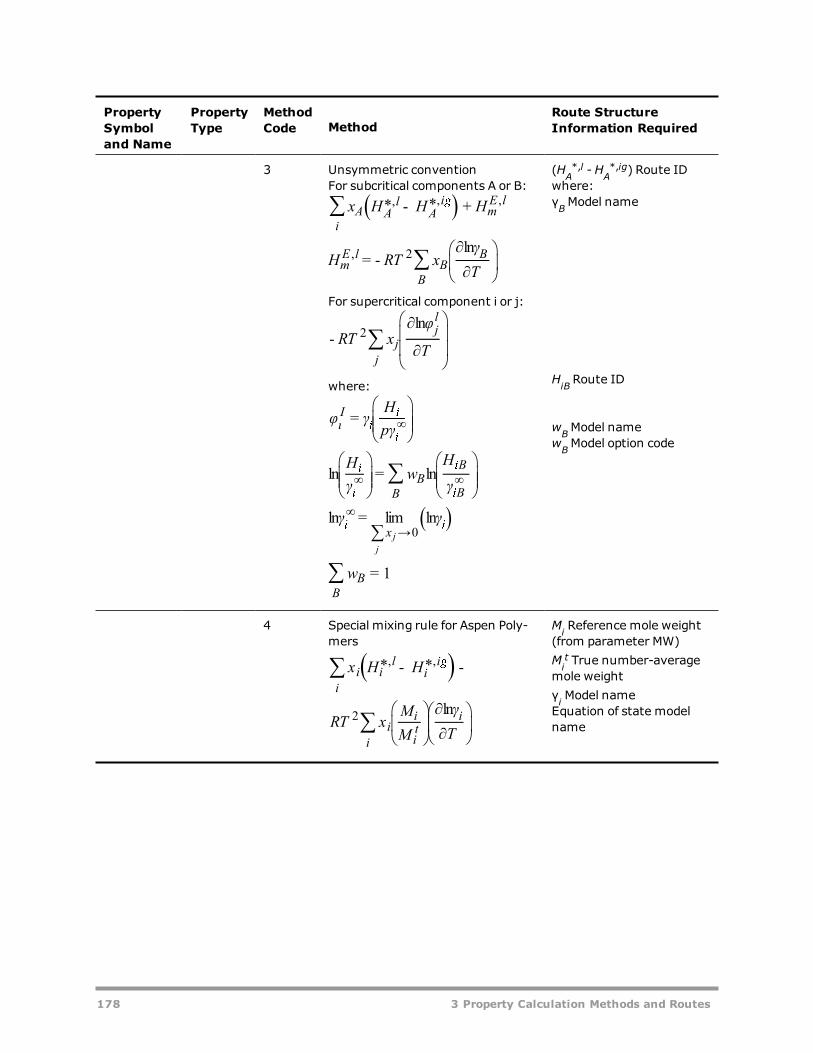
PropertySymboland Name
PropertyType
MethodCode Method
Route StructureInformation Required
3 Unsymmetric conventionFor subcritical components A or B:
( )∑
∑
x H H H
H RT xγ
T
* − * +
= −∂ln
∂
i
A Al
Ai�
mE l
mE l
B
BB
, , ,
, 2
For supercritical component i or j:
∑RT xφ
T−
∂ln
∂j
jjl
2
where:
( )
∑
∑
∑
φ γH
pγ
H
γw
H
γ
γ γ
w
=
ln = ln
ln = lim ln
= 1
ιΙ
�
�
�
�
� B
B�B
�B
�x
�
B
B
∞
∞ ∞
∞
→0
j
j
(HA*,l -HA
*,ig) Route IDwhere:γBModel name
HiB Route ID
wBModel namewBModel option code
4 Special mixing rule for Aspen Poly-mers
( )∑
∑
x H H
RT xM
M
γ
T
* − * −
∂ln
∂
i
i il
ii�
i
ii
it
i
, ,
2
Mi Reference mole weight(from parameter MW)Mit True number-average
mole weightγi Model nameEquation of state modelname
178 3 Property Calculation Methods and Routes

PropertySymboland Name
PropertyType
MethodCode Method
Route StructureInformation Required
5 Unsymmetric convention for AspenPolymersFor subcritical components A or B:
( )∑
∑
x H H H
H RT xM
M
γ
T
* − * +
= −∂ln
∂
i
A Al
Ai�
mE l
mE l
B
Bi
it
B
, , ,
, 2
For supercritical component i or j:
∑RT xφ
T−
∂ln
∂j
jjl
2
where:
( )
∑
∑
∑
φ γH
pγ
H
γw
H
γ
γ γ
w
=
ln = ln
ln = lim ln
= 1
ιΙ
�
�
�
�
� B
B�B
�B
�x
�
B
B
∞
∞ ∞
∞
→0
j
j
(HA*,l -HA
*,ig) Route IDwhere:γBModel nameMi Reference mole weight(from parameter MW)Mit True number-average
mole weight
HiB Route ID
wBModel namewBModel option code
6 Unsymmetric convention, as inmethod 3 but for electrolyte activ-ity coefficient property method
(HA*,l -HA
*,ig) Route IDγBModel nameHiB Route IDwBModel namewBModel option code
7 Calculated from liquid fugacity coef-ficient using electrolyte modelsGMENRTLQ & GMENRTLS
See ENRTL-RK or ENRTL-SR
HmE,l
HLXSSubord. 1 Specifiedmodel Hm
E,l Model name
2∑H RT x
γ
T= −
∂ln
∂mE l
i
ii, 2
γi Model name
3 Property Calculation Methods and Routes 179

PropertySymboland Name
PropertyType
MethodCode Method
Route StructureInformation Required
3 Method for Aspen Polymers only:
∑H RT xM
M
γ
T= −
∂ln
∂mE l
i
ii
it
i, 2
γi Model nameMi Reference mole weight(from parameter MW)Mit True number-average
mole weight
Solid Enthalpy Methods
PropertySymbolandName
PropertyType
MethodCode Method
Route Struc-tureInformationRequired
Hi*,s
HSMajor 1 Specifiedmodel Hi
*,s Model name
2 Hi*,ig + (Hi
*,s -Hi*,ig) (Hi
*,s -Hi*,ig)
Route ID
Hi*,s -
Hi*,ig
DHS
Subord. 1 Specifiedmodel (Hi*,s -Hi
*,ig)Model name
2 (Hi*,v(T,pi
*,s) -Hi*,ig(T))
- ΔsubHi*(T)
+ (Hi*,s(T,p) -Hi
*,s(T,pi*,s))
pi*,s Model name
(Hi*,v -Hi
*,ig)Route ID(Default:Hi
*,v -Hi*,ig = 0 )
ΔsubHi*(T) Model
name(Hi
*,s(T,p) -Hi*,s
(T,pi*,s)) Route
ID (Default:Hi*,s(T,p) -Hi
*,s
(T,pi*,s) = 0)
Hi*,s(T,p)
-Hi*,s
(T,pi*,s)
DHSPC
Subord. 1
∫ V TV
Tdp* −
∂ *
∂p
p
is i
s
p*
,,
is,
pi*,s Model name
Vi*,s Model name
Hms
HSMXMajor 1 Specifiedmodel Hm
s Model name
180 3 Property Calculation Methods and Routes
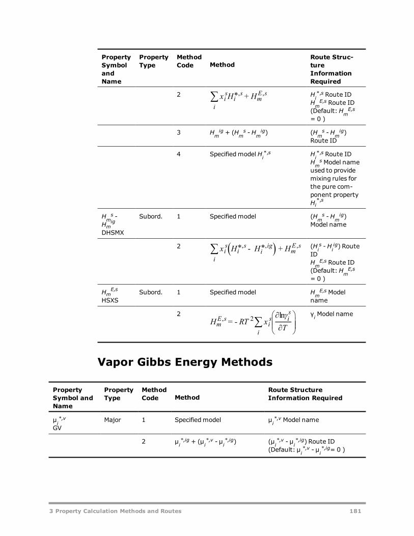
PropertySymbolandName
PropertyType
MethodCode Method
Route Struc-tureInformationRequired
2 ∑ x H H* +
i
i
s
i
s
m
E s, , Hi*,s Route ID
HmE,s Route ID
(Default:HmE,s
= 0 )
3 Hmig + (Hm
s -Hmig) (Hm
s -Hmig)
Route ID
4 Specifiedmodel Hi*,s Hi
*,s Route IDHm
s Model nameused to providemixing rules forthe pure com-ponent propertyHi*,s
Hms -
Hmig
DHSMX
Subord. 1 Specifiedmodel (Hms -Hm
ig)Model name
2 ( )∑ x H H H* − * +
i
is
is
iig
mE s, , , (Hi
s -Hiig) Route
IDHm
E,s Route ID(Default:Hm
E,s
= 0 )
HmE,s
HSXSSubord. 1 Specifiedmodel Hm
E,s Modelname
2∑H RT x
γ
T= −
∂ln
∂mE s
i
is i
s, 2
γi Model name
Vapor Gibbs Energy Methods
PropertySymbol andName
PropertyType
MethodCode Method
Route StructureInformation Required
μi*,v
GVMajor 1 Specifiedmodel μi
*,v Model name
2 μi*,ig + (μi
*,v - μi*,ig) (μi
*,v - μi*,ig) Route ID
(Default: μi*,v - μi
*,ig= 0 )
3 Property Calculation Methods and Routes 181

PropertySymbol andName
PropertyType
MethodCode Method
Route StructureInformation Required
μi*,v - μi
*,ig
DGVSubord. 1 Specifiedmodel (μi
*,v - μi*,ig) Model name
2RT φ RT
p
pln * + lniv
re�,
φi*,v Route ID
Gmv
GVMXMajor 1 Specifiedmodel Gm
vModel name
2 ∑ ∑y RT y yµ* + ln
ii i
v
ii i
, μi*,v Route ID
3 Gmig + (Gm
v -Gmig) (Gm
v -Gmig) Route ID
(Default:Gmv -Gm
ig= 0 )
4 Specifiedmodel μi*,v μi
*,v Route IDGm
v Model name used toprovide mixing rules for thepure component property μi
*,v
Gmv -Gm
ig
DGVMXSubord. 1 Specifiedmodel (Gm
v -Gmig) Model name
2∑RT y φ RT
p
pln + ln
ii i
vre�
φiv Route ID
(Default: φiv= 1 )
3 Gmv -Gm
ig = f(γi) γi Model nameEquation of state model name
Liquid Gibbs Energy Methods
PropertySymbol andName
PropertyType
MethodCode Method
Route StructureInformation Required
μi*,l
GLMajor 1 Specifiedmodel μi
*,l Model name
2 μi*,ig + (μi
*,l - μi*,ig) (μi
*,l - μi*,ig) Route ID
μi*,l - μi
*,ig
DGLSubord. 1 Specifiedmodel (μi
*,l - μi*,ig) Model name
182 3 Property Calculation Methods and Routes
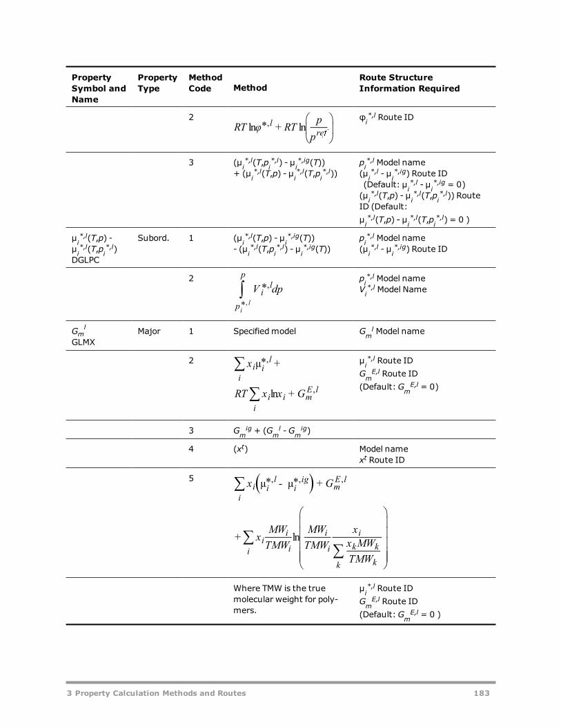
PropertySymbol andName
PropertyType
MethodCode Method
Route StructureInformation Required
2RT φ RT
p
pln * + ln
lre�
,
φi*,l Route ID
3 (μi*,l(T,pi
*,l) - μi*,ig(T))
+ (μi*,l(T,p) - μi
*,l(T,pi*,l))
pi*,l Model name
(μi*,l - μi
*,ig) Route ID(Default: μi
*,l - μi*,ig = 0)
(μi*,l(T,p) - μi
*,l(T,pi*,l)) Route
ID (Default:μi*,l(T,p) - μi
*,l(T,pi*,l) = 0 )
μi*,l(T,p) -
μi*,l(T,pi
*,l)DGLPC
Subord. 1 (μi*,l(T,p) - μi
*,ig(T))- (μi
*,l(T,pi*,l) - μi
*,ig(T))pi*,l Model name
(μi*,l - μi
*,ig) Route ID
2
∫ V dp*
p
p
il
*
,
il,
pi*,l Model name
Vi*,l Model Name
Gml
GLMXMajor 1 Specifiedmodel Gm
l Model name
2 ∑
∑
x
RT x x G
µ* +
ln +
i
i i
l
i
i i mE l
,
,
μi*,l Route ID
GmE,l Route ID
(Default:GmE,l = 0)
3 Gmig + (Gm
l -Gmig)
4 (xt) Model namext Route ID
5 ( )∑
∑∑
x G
xMW
TMW
MW
TMW
x
x MW
TMW
µ* − µ* +
+ ln
i
i il
iig
mE l
i
ii
i
i
i
i
k
k k
k
, , ,
Where TMW is the truemolecular weight for poly-mers.
μi*,l Route ID
GmE,l Route ID
(Default:GmE,l = 0 )
3 Property Calculation Methods and Routes 183

PropertySymbol andName
PropertyType
MethodCode Method
Route StructureInformation Required
6 Specifiedmodel μi*,l μi
*,l Route IDGm
l Model name used to providemixing rules for the pure com-ponent property μi
*,l
7 Gmig + (Gm
l -Gmig)
for electrolyte system
Gml -Gm
ig
DGLMX
Subord. 1 Specifiedmodel (Gml -Gm
ig) Model name
2 ( )∑ x Gµ* − µ* +
i
i il
iig
mE l, , , (μi
*,l - μi*,ig) Route ID
GmE,l Route ID
(Default:Gm
E,l= 0 )
3 ∑RT x φ
RT
ln +
ln
i
i il
p
pre�
φil Route ID
4 Gml -Gm
ig = f(γi) γi Model nameEquation of state model name
5 ∑RT x φ
RT
ln +
ln
i
i il
p
pre�
using electrolyte activitycoefficient model
φil Route ID
GmE,l
GLXSSubord. 1 Specifiedmodel Gm
E,l Model name
2 ∑RT x γln
i
i iγi Model name
3
∑ ∑RT xMW
TMWγ
TMW
MWxMW
TMWln + ln
i
ii
ii
i
i k
kk
k
Where TMW is the truemolecular weight for poly-mers.
γi Model name
184 3 Property Calculation Methods and Routes
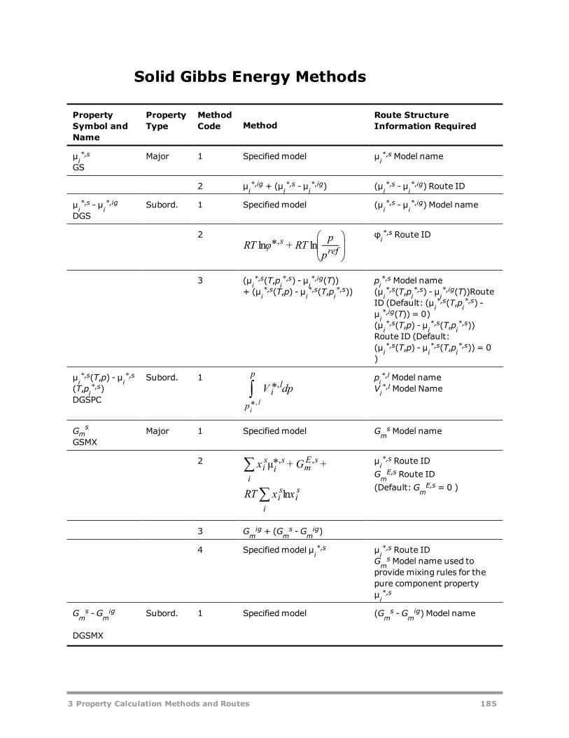
Solid Gibbs Energy Methods
PropertySymbol andName
PropertyType
MethodCode Method
Route StructureInformation Required
μi*,s
GSMajor 1 Specifiedmodel μi
*,s Model name
2 μi*,ig + (μi
*,s - μi*,ig) (μi
*,s - μi*,ig) Route ID
μi*,s - μi
*,ig
DGSSubord. 1 Specifiedmodel (μi
*,s - μi*,ig) Model name
2RT φ RT
p
pln * + ln
sre�
,
φi*,s Route ID
3 (μi*,s(T,pi
*,s) - μi*,ig(T))
+ (μi*,s(T,p) - μi
*,s(T,pi*,s))
pi*,s Model name
(μi*,s(T,pi
*,s) - μi*,ig(T))Route
ID (Default: (μi*,s(T,pi
*,s) -μi*,ig(T)) = 0)
(μi*,s(T,p) - μi
*,s(T,pi*,s))
Route ID (Default:(μi
*,s(T,p) - μi*,s(T,pi
*,s)) = 0)
μi*,s(T,p) - μi
*,s
(T,pi*,s)
DGSPC
Subord. 1
∫ V dp*
p
p
il
*
,
il,
pi*,l Model name
Vi*,l Model Name
Gms
GSMXMajor 1 Specifiedmodel Gm
s Model name
2 ∑
∑
x G
RT x x
µ* + +
ln
i
is
i
smE s
i
is
is
, , μi*,s Route ID
GmE,s Route ID
(Default:GmE,s = 0 )
3 Gmig + (Gm
s -Gmig)
4 Specifiedmodel μi*,s μi
*,s Route IDGm
s Model name used toprovide mixing rules for thepure component propertyμi*,s
Gms -Gm
ig
DGSMX
Subord. 1 Specifiedmodel (Gms -Gm
ig) Model name
3 Property Calculation Methods and Routes 185

PropertySymbol andName
PropertyType
MethodCode Method
Route StructureInformation Required
2 ( )∑ x Gµ* − µ* +
i
is
is
iig
mE s, , , (μi
*,s - μi*,ig) Route ID
GmE,s Route ID
(Default:GmE,s = 0 )
GmE,s
GSXSSubord. 1 Specifiedmodel Gm
E,s Model name
2 ∑RT x γln
i
is
is γi Model name
Vapor Entropy Methods
Property Symbol andName
PropertyType
MethodCode
Method Route StructureInformation Required
Si*,v
SVMajor 1
( )TH
1* − µ*i
v
i
v, , Hi*,v Route ID
2 Si*,ig + (Si
*,v -Si*,ig)
(Si*,v - Si
*,ig) Route ID(Default: Si
*,v - Si*,ig= 0 )
3 Specifiedmodel Si*,v Model name
Si*,v - Si
*,ig
DSVSubord. 1
−H H
T
T
* − *
µ* − µ*
iv
iig
iv
iig
, ,
, ,
(Hi*,v -Hi
*,ig) Route ID(Default:Hi
*,v -Hi*,ig= 0 )
(μi*,v - μi
*,ig) Route ID(Default: μi
*,v - μi*,ig= 0)
2( )
T−∂
∂µ* − µ*iv
iig, , (μi
*,v - μi*,ig) Model name
Specifiedmodel Si*,v - Si
*,ig Model name
Smv
SVMXMajor 1
TH G
1( − )mv
mv Hm
vRoute IDGm
vRoute ID
2 Smig + (Sm
v - Smig) (Sm
v - Smig) Route ID
(Default: Smv - Sm
ig= 0 )
3 Specifiedmodel Smv Model name
186 3 Property Calculation Methods and Routes

Property Symbol andName
PropertyType
MethodCode
Method Route StructureInformation Required
Smv - Sm
ig
DSVMXSubord. 1 Specifiedmodel (Sm
v - Smig) Model name
2 H H
T
G G
T
−−
−
mv
mig
mv
mig
(Hmv -Hm
ig) Route ID(Default:Hm
v -Hmig= 0 )
(Gmv -Gm
ig)Route ID(Default Gm
v -Gmig= 0)
3
TG G−
∂
∂( − )mv
mig (Gm
v -Gmig) Model name
4 Smv - Sm
ig = f(γi) γi Model nameEquation of state modelname
Liquid Entropy Methods
Property Symbol andName
PropertyType
MethodCode Method
Route StructureInformation Required
Si*,l
SLMajor 1 ( )
TH
1* − µ*il
i
l, , Hi*,l Route ID
μi*,l Route ID
2 Si*,ig + (Si
*,l - Si*,ig) (Si
*,l - Si*,ig) Route ID
3 Specifiedmodel Si*,l Model name
Si*,l - Si
*,ig
DSLSubord. 1 H H
T
T
* − *−
µ* − µ*
il
iig
il
iig
, ,
, ,
(Hi*,l -Hi
*,ig) Route ID
2 ( )T
−∂
∂µ* − µ*il
iig, , (μi
*,l - μi*,ig) Route ID
(μi*,l - μi
*,ig) Model name
3 Specified Model (Si*,l - Si
*,ig) Model name
Sml
SLMXMajor 1 ( )
TH G
1−ml
ml Hm
l Route IDGm
l Route ID
3 Property Calculation Methods and Routes 187
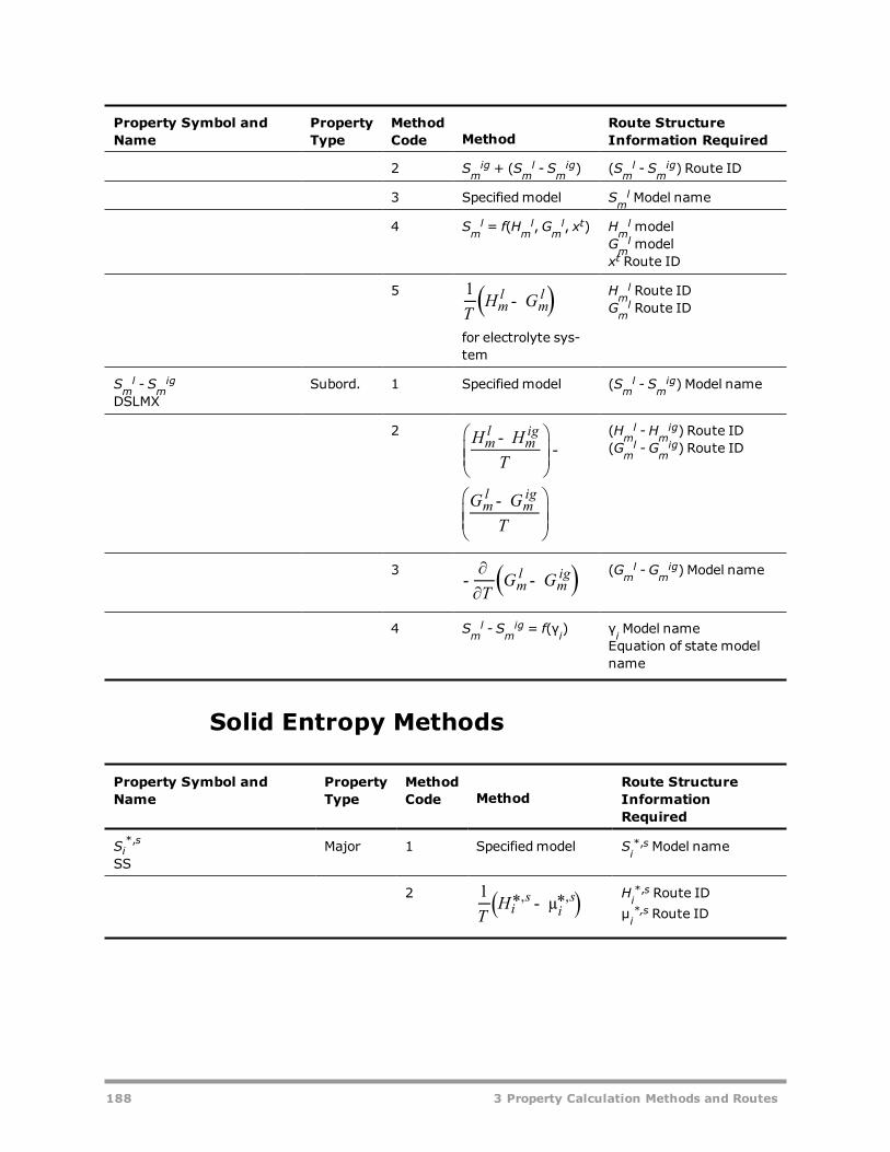
Property Symbol andName
PropertyType
MethodCode Method
Route StructureInformation Required
2 Smig + (Sm
l - Smig) (Sm
l - Smig) Route ID
3 Specifiedmodel Sml Model name
4 Sml = f(Hm
l,Gml, xt) Hm
lmodelGm
lmodelxt Route ID
5 ( )TH G
1−ml
ml
for electrolyte sys-tem
Hml Route ID
Gml Route ID
Sml - Sm
ig
DSLMXSubord. 1 Specifiedmodel (Sm
l - Smig) Model name
2 H H
T
G G
T
−−
−
ml
mig
ml
mig
(Hml -Hm
ig) Route ID(Gm
l -Gmig) Route ID
3 ( )TG G−
∂
∂−ml
mig (Gm
l -Gmig) Model name
4 Sml - Sm
ig = f(γi) γi Model nameEquation of state modelname
Solid Entropy Methods
Property Symbol andName
PropertyType
MethodCode Method
Route StructureInformationRequired
Si*,s
SSMajor 1 Specifiedmodel Si
*,s Model name
2( )
TH
1* − µ*i
s
i
s, , Hi*,s Route ID
μi*,s Route ID
188 3 Property Calculation Methods and Routes

Property Symbol andName
PropertyType
MethodCode Method
Route StructureInformationRequired
Si*,s - Si
*,ig
DSSSubord. 1 H H
T
T
* − *−
µ* − µ*
is
iig
is
iig
, ,
, ,
(Hi*,s -Hi
*,ig) Route ID(μi
*,s - μi*,ig) Route ID
2 Specifiedmodel (Si*,s - Si
*,ig) Modelname
Sms
SSMXMajor 1
TH G
1( − )ms
ms Hm
s Route IDGm
s Route ID
2 Smig + (Sm
s - Smig) (Sm
s - Smig) Route ID
Sms - Sm
ig
DSSMXSubord. 1 Specifiedmodel (Sm
s - Smig) Model name
2 H H
T
G G
T
−−
−
ms
mig
ms
mig
(Hms -Hm
ig) Route ID(Gm
s -Gmig) Route ID
3
TG G−
∂
∂( − )ms
mig (Gm
s -Gmig) Model
name
Molar Volume Methods
Property Symbol andName
PropertyType
MethodCode Method
Route StructureInformationRequired
Vi*,v
VVMajor 1 Specifiedmodel Vi
*,v Model name
Vmv
VVMXMajor 1 Specifiedmodel Vm
v Model name
2 Vmv = f(yi,Vi
*,v) Vi*,v Route ID
Vmv Model name
3 Property Calculation Methods and Routes 189

Property Symbol andName
PropertyType
MethodCode Method
Route StructureInformationRequired
3 Vmv = f(γi) γi Model name
γi Model name (eos only)
Vi*,l
VLMajor 1 Specifiedmodel Vi
*,l Model name
Vml
VLMXMajor 1 Specifiedmodel Vm
l Model name
2 Vml = f(xi,Vi
*,l) Vi*,l Route ID
Vml Model name
3 Electrolyte model(xt)
Vi*,l Model name
xt Route ID
4 Vml = f(γi) γi Model name
Vml Model name (eos
only)
Vi*,s
VSMajor 1 Specifiedmodel Vi
*,s Model name
Vms
VSMXMajor 1 Specifiedmodel Vm
s Model name
2 Vms = f(xi
s,Vi*,s) Vi
*,s Route IDVm
s Model name
Viscosity Methods
Property Symbol andName
PropertyType
MethodCode Method
Route StructureInformation Required
ηi*,v
MUVMajor 1 Specifiedmodel ηi
*,v Model name
2 ηi*,v = ηi
*,v (p=0) (ηi*,v (p=0)) Route ID
3 ηi*,v = f(Vi
*,v) Vi*,v Route ID
ηi*,v Model name
4 ηi*,v = ηi
*,v(p=0)+ (ηi
*,v(p) - ηi*,v(p=0))
(ηi*,v (p=0)) Route ID
(ηi*,v(p) - ηi
*,v(p=0))Route ID
ηi*,v(p=0)
MUVLPSubord. 1 Specifiedmodel (ηi
*,v (p=0)) Model name
190 3 Property Calculation Methods and Routes

Property Symbol andName
PropertyType
MethodCode Method
Route StructureInformation Required
ηi*,v(p) - ηi
*,v(p=0)MUVPC
Subord. 1 Specifiedmodel (ηi*,v(p) - ηi
*,v(p=0))Model name
2 (ηi*,v(p) - ηi
*,v(p=0)) =f(Vi
*,v)Vi*,v Route ID
Model name
ηvMUVMX
Major 1 Specifiedmodel ηv Model name
2 ηv = f(yi,ηi*,v) ηi
*,v Route IDηv Model name
3 ηv = ηv(p=0) (ηv (p=0)) Route ID
4 ηv = f(Vmv) Vm
v Route ID
5 ηiv = ηi
v(p=0)+ (ηi
v(p) - ηiv(p=0))
ηv Model name(ηv (p=0)) Route ID(ηi
v(p) - ηiv(p=0)) Route
ID
ηv (p=0)MUVMXLP
Subord. 1 Specifiedmodel (ηv (p=0)) Model name
2 (ηv (p=0)) = f(yi,ηi*,v
(p=0))(ηi
*,v (p=0)) Route ID(ηv (p=0)) Model name
ηv(p) - ηv(p=0)MUVMXPC
Subord. 1 Specifiedmodel (ηv(p) - ηv(p=0)) Modelname
2 (ηv(p) - ηv(p=0)) = f(Vm
v)Vm
v Route ID(ηv(p) - ηv(p=0)) Modelname
ηi*,l
MULMajor 1 Specifiedmodel ηi
*,l Model name
2 ηi*,l = f(Vi
*,l) Vi*,l Route ID
ηi*,l Model Name
ηlMULMX
Major 1 Specifiedmodel ηl Model name
2 ηl = f(xi,ηi*,l) ηi
*,l Route IDηl Model name
3 ηl = f(Vml) Vm
l Route IDηl Model name
4 Electrolyte model (xt) ηl Model namext Route ID
3 Property Calculation Methods and Routes 191

Thermal Conductivity Methods
Property Symbol andName
PropertyType
MethodCode Method
Route StructureInformation Required
λi*,v
KVMajor 1 Specifiedmodel λi
*,v Model name
2 λi*,v = (λi
*,v(p=0)) (λi*,v(p=0)) Route ID
3 λi*,v = (λi
*,v(p=0))+ (λi
*,v(p) - λi*,v(p=0))
(λi*,v(p=0)) Route ID
(λi*,v(p) - λi
*,v(p=0))Route ID
4 λi*,v = f(Vi
*,v, ηi*,v
(p=0))Vi*,v Route ID
(ηi*,v(p=0)) Model name
λi*,v Model Name
λi*,v(p=0)
KVLPSubord. 1 Specifiedmodel (λi
*,v(p=0)) Model name
2 λi*,v(p=0) = f(ηi
*,v
(p=0))(ηi
*,v(p=0)) Route IDλi*,v Model name
λi*,v(p) - λi
*,v(p=0)KVPC
Subord. 1 Specifiedmodel (λi*,v(p) - λi
*,v(p=0))Model name
2 (λi*,v(p) - λi
*,v(p=0)) =f(Vi
*,v)Vi*,v Route ID
(λi*,v(p) - λi
*,v(p=0))Model name
λvKVMX
Major 1 Specifiedmodel λv Model name
2 λv = f(yi, λi*,v) λi
*,v Route IDλv Model name
3 λv = (λv(p=0)) (λv(p=0)) Route ID
4 λv = (λv(p=0))+ (λv(p) - λv(p=0))
(λv(p=0)) Route ID(λv(p) - λv(p=0)) RouteID
5 λv = f(Vmv, ηv(p=0)) Vm
v Route ID(ηv(p=0)) Route IDλv Model name
λv(p=0)KVMXLP
Subord. 1 Specifiedmodel (λv(p=0)) Model name
2 λv(p=0) =f(yi, λi
*,v(p=0), ηi*,v
(p=0))
λi*,v Route ID
(ηi*,v(p=0)) Route ID
(λv(p=0)) Model name
192 3 Property Calculation Methods and Routes
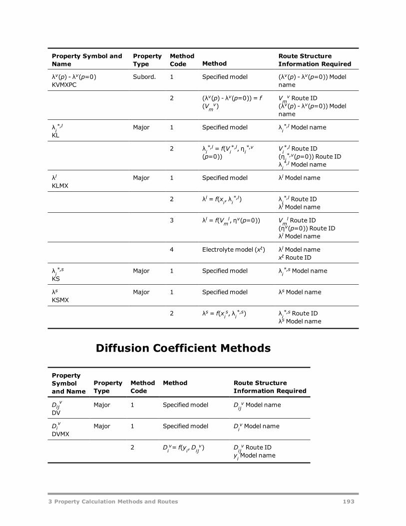
Property Symbol andName
PropertyType
MethodCode Method
Route StructureInformation Required
λv(p) - λv(p=0)KVMXPC
Subord. 1 Specifiedmodel (λv(p) - λv(p=0)) Modelname
2 (λv(p) - λv(p=0)) = f(Vm
v)Vm
v Route ID(λv(p) - λv(p=0)) Modelname
λi*,l
KLMajor 1 Specifiedmodel λi
*,l Model name
2 λi*,l = f(Vi
*,l, ηi*,v
(p=0))Vi*,l Route ID
(ηi*,v(p=0)) Route ID
λi*,l Model name
λlKLMX
Major 1 Specifiedmodel λl Model name
2 λl = f(xi, λi*,l) λi
*,l Route IDλl Model name
3 λl = f(Vml, ηv(p=0)) Vm
l Route ID(ηv(p=0)) Route IDλl Model name
4 Electrolyte model (xt) λl Model namext Route ID
λi*,s
KSMajor 1 Specifiedmodel λi
*,s Model name
λsKSMX
Major 1 Specifiedmodel λs Model name
2 λs = f(xis, λi
*,s) λi*,s Route ID
λs Model name
Diffusion Coefficient Methods
PropertySymboland Name
PropertyType
MethodCode
Method Route StructureInformation Required
Dijv
DVMajor 1 Specifiedmodel Dij
v Model name
Div
DVMXMajor 1 Specifiedmodel Di
v Model name
2 Div= f(yi,Dij
v) Dijv Route ID
yi Model name
3 Property Calculation Methods and Routes 193
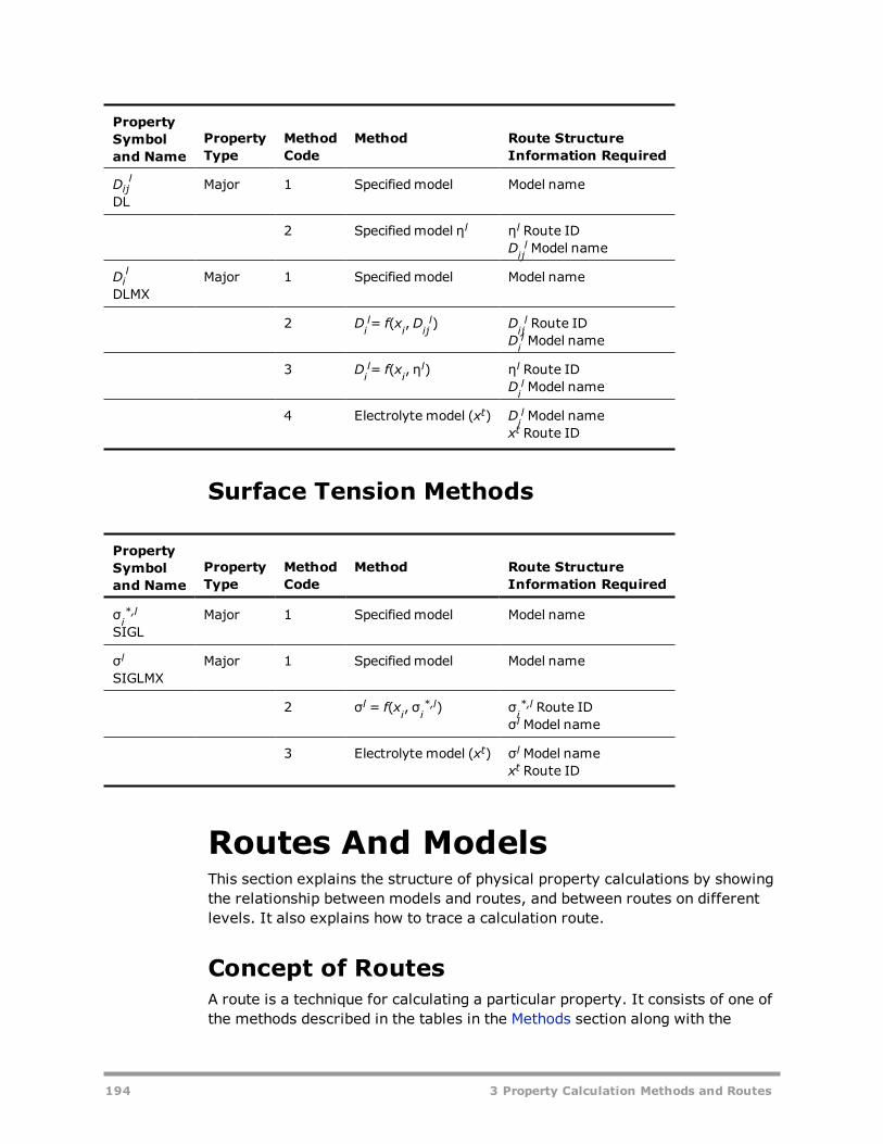
PropertySymboland Name
PropertyType
MethodCode
Method Route StructureInformation Required
Dijl
DLMajor 1 Specifiedmodel Model name
2 Specifiedmodel ηl ηl Route IDDijl Model name
Dil
DLMXMajor 1 Specifiedmodel Model name
2 Dil= f(xi,Dij
l) Dijl Route ID
Dil Model name
3 Dil= f(xi, η
l) ηl Route IDDil Model name
4 Electrolyte model (xt) Dil Model name
xt Route ID
Surface Tension Methods
PropertySymboland Name
PropertyType
MethodCode
Method Route StructureInformation Required
σi*,l
SIGLMajor 1 Specifiedmodel Model name
σlSIGLMX
Major 1 Specifiedmodel Model name
2 σl = f(xi, σi*,l) σi
*,l Route IDσl Model name
3 Electrolyte model (xt) σl Model namext Route ID
Routes And ModelsThis section explains the structure of physical property calculations by showingthe relationship between models and routes, and between routes on differentlevels. It also explains how to trace a calculation route.
Concept of RoutesA route is a technique for calculating a particular property. It consists of one ofthe methods described in the tables in the Methods section along with the
194 3 Property Calculation Methods and Routes

information needed to perform that calculation.
The technique contained in a route may depend on other properties. If a routerequires a major or subordinate property, then an additional, sub-level route isspecified within the route for calculating that other property. If a route requiresan intermediate property, then the model required for calculating that propertyis specified within the route. A route may also simply consist of a model that dir-ectly calculates the property. If a model used in a route has model optioncodes, these are specified in the route as well.
The collection of all this information is called a route. Since routes can dependon other routes, and those routes may in turn depend on yet other routes, amulti-level tree of routes may exist under a single route. Example 1 discusses aroute that does not depend on other routes. See Example 2 for a route whichdepends on a secondary route.
Models consist of the equations needed to calculate a property from state vari-ables and parameters. They do not depend on other routes, and make up theend branches of the tree of routes.
Each built in route in the Aspen Physical Property System has a unique route ID,which is composed of the property name (as described in the tables of MajorProperties, Subordinate Properties, and Intermediate Properties) and a num-ber, for example HLMX10.
Route IDs associated with the route information represent a unique com-bination of sub-level routes and models. Therefore, a top-level route ID spe-cifies the full calculation tree. Because of the uniqueness of route IDs, you canuse them for documenting your calculation. See Tracing a Route to learn how tofollow the tree of routes, and see an example of such a tree.
A property method can calculate a fixed list of properties (see Physical Prop-erties in the Aspen Physical Property System). The calculation procedure ofeach property constitutes a route and has a route ID. Therefore, a propertymethod consists of a collection of the route IDs of the properties it can cal-culate. The Methods | Selected Methods | Routes sheet shows the routesused in a property method. If you want to see all of the built-in routes availablefor calculating a property listed in the Property column, open the list in the cor-responding Route ID field. Select any route on this sheet and click View to seethe tree of routes and models under this route.
3 Property Calculation Methods and Routes 195
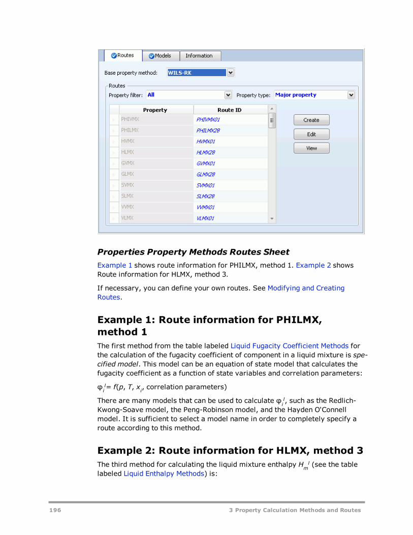
Properties Property Methods Routes SheetExample 1 shows route information for PHILMX, method 1. Example 2 showsRoute information for HLMX, method 3.
If necessary, you can define your own routes. See Modifying and CreatingRoutes.
Example 1: Route information for PHILMX,method 1The first method from the table labeled Liquid Fugacity Coefficient Methods forthe calculation of the fugacity coefficient of component in a liquid mixture is spe-cified model. This model can be an equation of state model that calculates thefugacity coefficient as a function of state variables and correlation parameters:
φil= f(p, T, xi, correlation parameters)
There are many models that can be used to calculate φil, such as the Redlich-
Kwong-Soave model, the Peng-Robinson model, and the Hayden O'Connellmodel. It is sufficient to select a model name in order to completely specify aroute according to this method.
Example 2: Route information for HLMX, method 3The third method for calculating the liquid mixture enthalpy Hm
l (see the tablelabeled Liquid Enthalpy Methods) is:
196 3 Property Calculation Methods and Routes

Hml = Hm
ig + (Hml - Hm
ig)
In this method, Hml depends on the ideal gas enthalpy and the enthalpy depar-
ture Hml - Hm
ig , a subordinate property. The table labeled Liquid Enthalpy Meth-ods indicates in the rightmost column that the required information is the routeID for the subordinate property. Specifying this route means that the top-levelroute now refers to a sub-level route ID.
For all methods that use both an ideal gas contribution and a departure func-tion, the Aspen Physical Property System automatically fills in the ideal gas cal-culation. You need to specify only the departure function.
To specify the sub-level route for the enthalpy departure, you must choose amethod. For example, you might choose method 1: specified model (see thetable labeled Liquid Enthalpy Methods). For this method, the required inform-ation is the model name, such as the Redlich-Kwong-Soave equation-of-statemodel.
ModelsA model consists of one or more equations to evaluate a property, and hasstate variables, universal parameters, and correlation parameters as input vari-ables. In contrast to methods (as described in Concept of Routes, above) whichare based only on universal scientific principles, models are much more arbit-rary in nature, and often have constants which need to be determined by datafitting. An example of a model is the Extended Antoine vapor pressure equation(see Physical Property Models). Equations of state have built in correlation para-meters and are also models.
Models are sometimes used in multiple routes of a property method. Forexample, an equation-of-state model can be used to calculate all vapor andliquid departure functions of an equation-of-state based property method. TheRackett model can be used to calculate the pure component and mixture liquidmolar volumes, (Vi
*,l and Vml), and it can also be used in the calculation of the
Poynting correction factor, as part of the calculation of the pure componentliquid fugacity coefficient.
The Methods | Selected Methods | Models sheet (shown below) displaysthe models that are globally used in the routes of the selected property method.Changing routes on the Methods | Selected Methods | Routes sheet causesthe Models sheet to be rewritten based on the new set of routes, so you shouldspecify all routes before specifying any models on the Models sheet.
Sometimes, different routes in a method which calculate the same property(one or both as intermediate steps in calculating some other property) may usedifferent models to calculate the property. In that case, the property will be lis-ted more than once on the Models sheet, with each applicable model listed.
For a given model, click the Affected properties button to display a list ofproperties which are affected by the model calculations. Open the list in a
3 Property Calculation Methods and Routes 197

Model Name field to display a list of all available models for a specific prop-erty.
Note: Changing amodel on this sheet causes it to be used for all properties which it cancalculate, overriding the methods specified by routes. If a property appears more thanonce, changing the model here affects calculation for all instances of the property. To spe-cify models only for specific properties, use routes instead. If necessary, you can createyour own routes; see Modifying and Creating Routes for details.
You can also use the tables labeled Thermodynamic Property Models, TransportProperty Models, and Nonconventional Solid Property Models in Physical Prop-erty Models. If you need to use a proprietary model or a new model from the lit-erature, you can interface these to the Aspen Physical Property System (seeAspen Plus User Models.)
Methods | Selected Methods | Models Sheet
Some models have model option codes to specify different possible calculationoptions. For example, the model WHNRY has three options to calculate theweighting factor from the critical molar volume. The calculation option is iden-tified by the model option code. On the Selected Methods | Models sheet,first select the model, then click the Option codes button to display a list ofoption code values for the model. See Property Model Option Codes in PhysicalProperty Models for descriptions of the option codes.
198 3 Property Calculation Methods and Routes
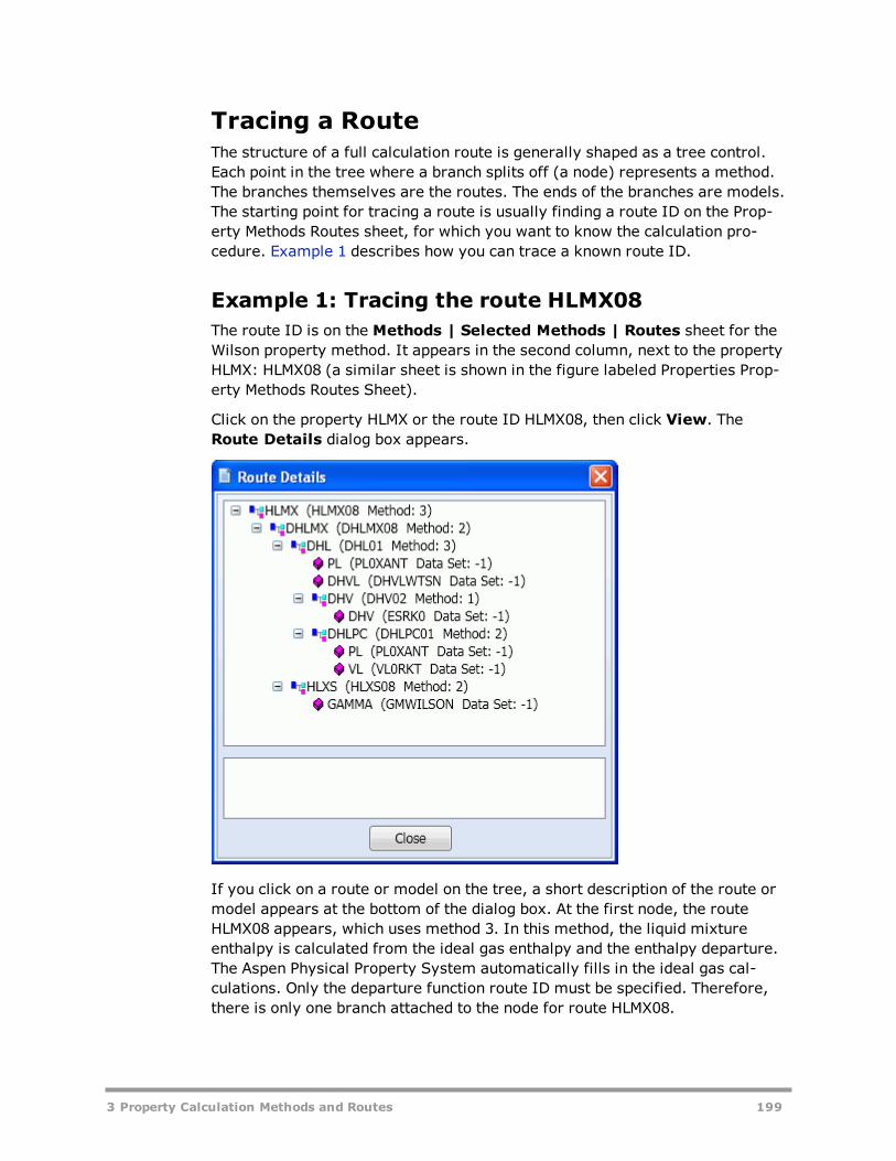
Tracing a RouteThe structure of a full calculation route is generally shaped as a tree control.Each point in the tree where a branch splits off (a node) represents a method.The branches themselves are the routes. The ends of the branches are models.The starting point for tracing a route is usually finding a route ID on the Prop-erty Methods Routes sheet, for which you want to know the calculation pro-cedure. Example 1 describes how you can trace a known route ID.
Example 1: Tracing the route HLMX08The route ID is on the Methods | Selected Methods | Routes sheet for theWilson property method. It appears in the second column, next to the propertyHLMX: HLMX08 (a similar sheet is shown in the figure labeled Properties Prop-erty Methods Routes Sheet).
Click on the property HLMX or the route ID HLMX08, then click View. TheRoute Details dialog box appears.
If you click on a route or model on the tree, a short description of the route ormodel appears at the bottom of the dialog box. At the first node, the routeHLMX08 appears, which uses method 3. In this method, the liquid mixtureenthalpy is calculated from the ideal gas enthalpy and the enthalpy departure.The Aspen Physical Property System automatically fills in the ideal gas cal-culations. Only the departure function route ID must be specified. Therefore,there is only one branch attached to the node for route HLMX08.
3 Property Calculation Methods and Routes 199

The next step in the route HLMX08 is the calculation of the liquid mixtureenthalpy departure with route ID: DHLMX08. This calculation is based onmethod 2, which calculates DHLMX as the mole fraction average of pure com-ponent enthalpy departure (DHL) and the excess enthalpy (HLXS). Therefore,two branches split from this route. The complete route can be traced this way.
These two steps in tracing the route HLMX08 show that a route ID is char-acteristic for the methods, routes and models specified on its own level.However, by specifying DHLMX08 on the top level, the top level route is alsocharacteristic for the level below because DHLMX08 stands for a full spe-cification on its secondary level. If we continue this reasoning down the tree tothe models, then it becomes clear that HLMX08 represents the full specificationof the full tree. And DHLMX08 represents the full specification of the full tree,minus the top level. Therefore every built in route has a unique ID. This featurewill be used in Modifying and Creating Routes.
Method NumbersTo look up the equation corresponding to the method number of a route, look upthe method in the table Methods tables. For instance, find HLMX in the tablelabeled Vapor Fugacity Coefficient Methods. The formula is listed next to themethod number.
Modifying and Creating Prop-erty MethodsThe built in property methods in the Aspen Physical Property System containchoices of major property routes that fit most engineering needs. The com-binations of the routes for different properties are chosen in a logical way, asexplained in Classifications of Property methods and Recommended Use in Prop-erty Method Descriptions. You may sometimes need to customize propertymethods. For example, to change models or routes on a main or a sub level.This section explains how to do this and gives examples of how to implementthe most frequently used modifications.
Modifying Existing Property MethodsThe following subsections explain the different types of modifications that canbe made to property methods.
l Replacing Routesl Replacing Models and Using Multiple Data Setsl Conflicting Route and Model Specifications
Replacing Routes
200 3 Property Calculation Methods and Routes

The Selected Methods | Routes sheet allows you to see which routes areused in a certain property method and to trace a route (see Routes andModels). This form also allows you to replace routes. A route replacement influ-ences the calculations of one property at a time.
To replace routes:
1. In the navigation pane, openMethods, then click Selected Methods.The Selected Methods Object Manager appears.
2. Select the property method and click Edit.The Selected Methods form appears.
3. Go to the Routes sheet.4. In the Route ID field of the property of interest, click to list all available
routes for this property.As you scroll through the list, the prompt displays a short description ofthe route. When you gain experience, the description from the promptshould be sufficient. If you require more information,
Select the route, then click the View button to get the tree dia-gram for this route (see Routes and Models). You can now tracethe route in detail.Close the View Route dialog box to return to the Routes sheet.
5. Select a route that fits your needs.The newly selected route changes color, so that you are able to locateyour property method modifications immediately on this sheet.
The technique is identical for subordinate properties.
Example 1: Using COSTALD liquid molar volume inPENG-ROBIn the PENG ROB property method, the Rackett equation is used for the liquidmolar volume (route VLMX01, property VLMX). For high pressure calculations,use the COSTALD model which is suited for compressed liquids. The route selec-ted is VLMX22. For consistency with pure component results, replace the VL cal-culation with VL06.
Example 2: Using Lee-Kesler liquid volume in RK-SoaveFor a high pressure hydrocarbon application, use the Lee Kesler liquid molarvolume calculation rather than the atmospheric API density calculation. SelectVLMX13 for VLMX. No corresponding pure component routes are available,since these calculations are for complex petroleum mixtures, of which the purecomponents are only partially known.
3 Property Calculation Methods and Routes 201

Example 3: Using ideal mixing for the liquid molarvolume in WILSONYou want to compare the Rackett mixture equation with ideal mixing. The purecomponent liquid molar volume should remain as it is (Model: VL0RKT, RouteID: VL01). Select the route VLMX23 to use the ideal mixing rule (mole fractionaverage of pure component liquid molar volumes).
Example 4: Removing Poynting correction of anactivity coefficientThe Poynting correction is the pressure correction to the pure component liquidfugacity coefficient. For validation purposes, you need to compare your cal-culation with previous results that have been obtained without the Poynting cor-rection.
In all activity coefficient based property methods with the Redlich Kwong equa-tion of state as the vapor phase model, the route PHIL04 is used for the purecomponent liquid fugacity coefficient. Tracing PHIL04 (using the View button)shows that the pressure correction is calculated by the subordinate propertyPHILPC with route ID PHILPC01.
On the Selected Methods | Routes sheet, select Subordinate property inthe Property route field. Locate the property PHILPC in the Property field,then replace PHILPC01 with PHILPC00 (no correction) in the Route ID field.If you trace PHIL04 again (using the View button), you will notice that the treeis dynamic; it reflects the changes you made in a sub level route, in this casefor PHILPC.
In the activity coefficient based property methods with the ideal gas law as thevapor phase model, the route PHIL00 is used. Tracing PHIL00 shows thatPHILPC00 is used by default. No changes are needed.
Replacing Models and Using Multiple Data SetsThe Selected Methods | Models sheet allows you to see which models areused in a certain property method (see Routes and Models). This sheet alsoallows you to replace models. Route replacements influence only one propertyat a time. In contrast, a model replacement influences all the properties thatuse the same model. You can trace the routes of these properties to determinewhere exactly the model is used in the calculation. If you want to limit theeffect of a model replacement to a single route, you can modify an existingroute or create a new route (see Modifying and Creating Routes). Click theAffected properties button to see a list of properties affected by the model.
If you need to change both routes and models, you must change the routes firstusing the Routes sheet, then change the models. If you use the Models sheetbefore using the Routes sheet, the changes you made on the Models sheet willbe lost.
202 3 Property Calculation Methods and Routes

To replace models:
1. In the navigation pane, openMethods, then click Selected Methods.The Selected Methods Object Manager appears.
2. Select the property method and click Edit.The Selected Methods form appears.
3. Go to the Models sheet.4. On the Model name field of the property of interest, click to see all
available models for this property. (You can also use the table labeledLiquid Fugacity Coefficient Methods.)As you scroll through the list, the prompt displays a short description ofthe model.
5. Select a model.The newly selected model changes color, so that you are able to locateyour property method modifications immediately on this form. All prop-erties using the same model will also be changed.
If you draw a tree diagram of a property in which the new model is used, themodification is also shown (see Tracing a Route).
Conflicting Route and Model SpecificationsIf you specify a route for a certain property and you also specify a model thatcalculates a property that is part of the route you specified, the information canbe conflicting. In the Aspen Physical Property System both replacements will beexecuted. The result, in most cases, is that the model takes precedence, butyou can always predict the result by analyzing the route and checking if there isan occurrence of this type of model in the tree.
Example 1 describes how to use COSTALD liquid molar volume in PENG-ROB.Example 2 describes how to use Peng Robinson for vapor phase properties inNRTL RK.
Example 1: Using COSTALD liquid molar volume inPENG-ROB: Replacing ModelsThe reasoning is the same as in Example 1, Replacing Routes. The approachhere is to replace the Rackett models (VL0RKT, VL2RKT) by the COSTALD mod-els (VL0CTD, VL2CTD). The result is exactly the same as for the route replace-ment.
Example 2: Using Peng-Robinson for vapor phaseproperties in NRTL-RKYou want to use the Peng Robinson equation of state as the vapor phase modelof an activity coefficient based property method. Instead of replacing every
3 Property Calculation Methods and Routes 203
vapor phase property route, it is more efficient to replace the equation of statemodel used for all vapor phase properties. In the model field, if you selectESPR for a single vapor phase property, the Aspen Physical Property Systemreplaces all other vapor phase properties by the ESPR model as well. For con-sistency, use ESPR0 for pure component vapor phase properties.
Creating New Property MethodsThe purpose of creating new property methods is not so much to build the col-lection of routes from scratch, although this is possible. It is more a matter ofmethodology and documentation of your work. Suppose you make changes toexisting property methods, and you have successfully completed your cal-culations. One year later you may have a similar project where you begin withyour old calculation models. You may not remember that the WILSON propertymethod you used is not the standard version. Therefore, it is recommendedthat you:
1. Create a new property method with an ID similar to the property methodon which it is based.
2. Copy the base property method to the new property method3. Make your changes.
There are two ways to begin the creation of a property method.
The first way to begin is:
1. On the Methods | Specifications | Global sheet, select the base prop-erty method on the Base method field.
2. Check the Modify property models checkbox. The Modify PropertyMethod dialog box appears.
3. Enter the new property method name, then click OK.4. Go to the Methods | Selected Methods Object Manager.5. Select the new property method, then click Edit.
The second way to begin is:
1. Go to the Methods | Selected Methods Object Manager.2. Click New and enter the new property method name.
The Selected Methods form for the new method appears.
Then for both methods do the following steps:
1. Select the Routes sheet or the Models sheet.2. On the Base property method field, select an existing property
method name.The Aspen Physical Property System fills in all the routes and models inboth sheets.
3. Make your changes.
204 3 Property Calculation Methods and Routes

4. Use the newly created property method in a flowsheet, a block, a prop-erty analysis, or a column section.
Using Multiple Data Sets in Multiple Property Meth-odsTo use a second data set with a model:
1. From the navigation pane, openMethods, then click Selected Meth-ods.The Selected Methods Object Manager appears.
2. Select the property method and click Edit.The Selected Methods form appears.
3. Go to the Models sheet.The Data Set column is to the right of the Model name column. Thedefault for a data set number is 1.
4. Change the data set number to 2 to introduce a second set of parametersfor a model.
A second data set is frequently used for activity coefficient models. Forexample, the VLE are calculated with one set of parameters, the LLE withanother set. If you introduce a second data set for an activity coefficient model,it is effective throughout the property method. To use two data sets in differentparts of the flowsheet or a distillation column, you must use two property meth-ods: one property method that uses the default data set 1, and another prop-erty method that uses the data set 2. If you create a second data set for amodel, the Aspen Physical Property System automatically defines the secondset of parameters on the Methods | Parameters forms. So you must enterthe parameters values for the second data set after creating the propertymethod in which they are to be used.
There are a few pre-defined property methods which use data set 2: NRTL-2,UNIQ-2, VANL-2, and WILS-2. When you add one of these property methods toyour simulation, the binary parameter form for the data set it uses is addedunder Methods| Parameters.
Note: Data regression runs can only manipulate the first data set. You can copy para-meters obtained through data regression into any other data set and then use that dataset during simulation runs.
Modifying and Creating RoutesThe built in routes in the Aspen Physical Property System cover most engin-eering needs (see Routes and Models). However, while modifying or creatingproperty methods you may need a route that is not built in (see Modifying andCreating Property Methods). You can create such a route based on the available
3 Property Calculation Methods and Routes 205

methods. This section explains and gives examples of modifying and creatingroutes.
To decide if you want to create a new route or modify an existing route, applythe same reasoning as for deciding whether to modify or create a new propertymethod (see Creating New Property Methods). We recommend you choose anew route ID.
To modify an existing route or create a new route:
1. Follow the procedure to trace routes, and consider the available methodsfor the property of interest. Decide on the route you want to modify, orthe method you want to use to create a route.
2. In the navigation pane, openMethods, then click Routes.The Routes Object Manager appears. There are no objects listedbecause there are hundreds of available routes. So you need to knowfrom the analysis you did on the Selected Methods | Routes sheetwhich route you want to modify.
3. Click New. Enter a new route ID to create a new route, or enter an exist-ing route ID to modify an existing route.The Routes | Specifications sheet appears. At the top are the:
Property nameMethod code (described in Methods earlier in this chapter)Route ID of the route to modify
4. When you base your new route on an existing route, enter the propertyname in the Property name field and the base route ID in the Copyroute from field, and make your changes.OrWhen you create a completely new route, enter the property name andmethod code. Fill the Route ID andModel name fields.
5. Use the Selected Methods | Routes sheet and enter the new route ina property method.OrUse the Routes | Specifications sheet of another route to use thenewly created route in another route.
Example 1 describes how to use a second data set of NRTL parameters forHLXS. Example 2 describes how to use your own model for the liquid enthalpy.
Example 1: Use a second data set of NRTLparametersThe representation of two properties with one data set is sometimes not sat-isfactory, for example with VLE and excess enthalpy data. If two data sets candescribe the properties separately, you will need to use both sets in the cal-culation.
206 3 Property Calculation Methods and Routes

In this example, one set of binary parameters for the NRTL model is used forVLE calculations. A second set of binary parameters is used for excess enthalpy(HLXS).
Create a new route to calculate HLXS. The simplest way is to modify the exist-ing route used in the NRTL property method. The Route ID is HLXS10. On theMethods | Routes | Specification sheet, change Data Set from 1 to 2.
Example 2: Using your own model for theliquid enthalpyYour company has developed a correlation for the enthalpy in a specific processstream that you want to use. The necessary user model subroutines have beenwritten according to Aspen Plus User Models. All built in routes in the AspenPhysical Property System for the liquid molar enthalpy are based on methods 2,3 or 4. However, to use the user model, method 1 (Specified model) is needed.Because no existing route uses method 1 or needs this type of model, there isno model for liquid enthalpy on the Selected Methods | Models sheet.
Create a new route, for example HLMXAP, using method 1. On the Routes |Specifications sheet. the property name HLMX appears in the Model area.Click the Model name field and select HL2USR, the liquid mixture enthalpyuser model.
Reference the route HLMXAP in the property method on the Selected Methods| Routes sheet. You can check that the user enthalpy model HL2USR appearson the Selected Methods | Models sheet.
3 Property Calculation Methods and Routes 207

208 3 Property Calculation Methods and Routes

4 Electrolyte Calculation
Electrolyte process calculation has many applications. In the Aspen PhysicalProperty System, you can analyze and optimize processes involving ionic spe-cies, complex ions, salt precipitation, with strong acids, weak acids and bases.
Examples of applications for electrolyte process calculation with the Aspen Phys-ical Property System include:
l Sour water stripping (petrochemical industry)l Caustic brine evaporation and crystallization (chlor-alkali industry)l Acid gas removal (chemical and gas industries)l Nitric acid separation (nuclear chemical industry)l Trona processing (mining industry)l Organic salt separation (biochemical industry)l Black liquor evaporation (pulp and paper industry)
Electrolyte systems have three important characteristics:
l Solution chemistry in the liquid phasel Apparent and true component compositions are differentl Non-ideal liquid phase thermodynamic behavior
This chapter describes applications of electrolyte process calculation andreviews the following fundamental characteristics of electrolyte systems:
l Solution chemistryl Apparent component and true component approachesl Aqueous electrolyte chemical equilibriuml Electrolyte thermodynamics modelsl Electrolyte data regression
Solution ChemistryThe solution chemistry involves a variety of chemical reactions in the liquidphase. Examples of such chemical reactions are:
4 Electrolyte Calculation 209

l Complete dissociation of strong electrolytesl Partial dissociation of weak electrolytesl Ionic reactions among ionic speciesl Complex ion formationl Salt precipitation and dissolution
These chemical reactions occur rapidly in solution, so chemical equilibrium con-ditions are assumed.
Solution chemistry affects electrolyte process calculation by influencing phys-ical properties, phase equilibrium, and other fundamental characteristics ofelectrolyte systems. For most nonelectrolyte systems, chemical reactionsoccur only in reactors. For electrolyte systems, chemical equilibrium cal-culations are essential to all types of unit operations modeling.
Solution chemistry dictates the true components in solution and imposes equal-ity constraints on their composition. The chemical equilibrium relationship forreaction j is expressed as:
∑K v aln = lnj
i
i j i,(1)
Where:
Kj = Chemical equilibrium constant
vi,j = Reaction stoichiometric coefficient of component i
ai = Activity of component i
Computation of the solution chemistry is often combined with phase equilibriumcalculations. Typical electrolyte calculations involving solution chemistry are:
l Liquid (aqueous) phase equilibrium (for example, calculating the pH forthe titration of organic acid with caustic solution)
l Vapor-liquid (aqueous) phase equilibrium (for example, extractive dis-tillation with salts as extractive agents, and sour water stripping)
l Liquid (aqueous)-liquid (organic) phase equilibrium (for example, hydro-carbon-sour water system and liquid-liquid extraction of metals)
l Liquid (aqueous)-solid equilibrium of salt precipitation (for example,crystallization of organic or inorganic salts)
To simulate an electrolyte system, you must properly identify all relevant chem-ical reactions. Physical interactions in solutions are sometimes described bypostulating chemical reactions at equilibrium. The chemical theory of solutionsis used only for real chemical reactions. Incorrect assumptions about the solu-tion chemistry is the major cause of inaccuracies in calculations of reactivechemical systems.
210 4 Electrolyte Calculation

Use the Electrolyte Expert System to identify all relevant chemical reactions.Starting from this set of reactions, you can remove and/or add reactions asrequired to properly represent your process.
You can use the Chemistry form to describe the solution chemistry and toenter the chemical equilibrium constants. However, we strongly recommendthat you use the Elec Wizard on the Components | Specifications | Selec-tion sheet and allow the Electrolyte Expert System to set up the property spe-cifications for you.
For a system with a solvent dielectric constant less than 10, ionic reactions donot take place. Therefore, the Aspen Physical Property System bypasses allsolution chemistry calculations for such systems.
If you define the reactions on the Chemistry form, the Aspen Physical Prop-erty System checks for infeasible or redundant reactions. If such reactionsexist, the Aspen Physical Property System ignores them during the calculations.
Apparent Component and TrueComponent ApproachesAs a result of the solution chemistry, a set of true species is present in theliquid phase that differs from apparent molecular components. Apparent or par-ent components are present in the system if no reactions occurred. Forexample, the sour water stripper system has three apparent molecular com-ponents: water, ammonia, and hydrogen sulfide. The three molecular com-ponents dissociate in the liquid phase.
There are four ionic reactions:
H O H O OH2 ↔ +2 3+ − (2)
NH H O NH OH+ ↔ +3 2 4+ − (3)
H S H O H O HS+ ↔ +2 2 3+ − (4)
HS H O H O S+ ↔ +−
2 3+ − 2 (5)
Five ionic species are thereby produced from these aqueous phase ionic reac-tions. All components in these reactions exist at chemical equilibrium con-ditions and are the true components of the electrolyte system. The apparentcomponents are H2O, NH3, and H2S.
These two sets of components have major effects on the treatment of elec-trolyte process calculation. Apparent components are of major concern to someelectrolyte processes since process measurements are usually expressed interms of apparent components. To other electrolyte processes, expression in
4 Electrolyte Calculation 211

terms of true species is the only way to characterize an electrolyte system. Theselection of apparent components or true components therefore depends on thetype of electrolyte system you simulate.
Three types of molecular components may be present in an electrolyte system:solvents, molecular solutes, and electrolytes. As a result of electrolyte solutionchemistry, ions, salts, and nonvolatile molecular solutes may be present asadditional true species. These components are defined as:
l Solvent: water is the solvent for aqueous electolyte systems. For mixed-solvent electrolyte systems, there are other solvent components in addi-tion to water.
l Molecular solutes are molecular species, other than solvent compounds,that exist in the liquid phase in molecular form. All molecular solutes aretreated with Henry's law. They are often supercritical components.
l Electrolytes are also molecular species. However, strong electrolytes dis-sociate completely to ionic species in the liquid phase. Undissociatedweak electrolytes can be solvent components or molecular solutes.
l Ions are nonvolatile ionic species that exist only in the liquid phase.l Salts are nonvolatile molecular species that exist as solids.
Choosing the True or Apparent ApproachThe apparent component approach and the true component approach are inter-changeable because liquid solution chemistry based on apparent componentcomposition defines the true component composition of a system. The AspenPhysical Property System calculates thermodynamic properties of componentsand mixtures expressed in terms of apparent component composition fromproperties expressed in terms of true component composition. For example,the liquid fugacity coefficient of ammonia with the apparent componentapproach is calculated from the liquid fugacity coefficient of ammonia with thetrue component approach:
φ φx
x=
ia l
it l i
t
ia
, ,(6)
Where:
φia l, = Fugacity coefficient of apparent component i
φit l, = Fugacity coefficient of true component i
xi = Liquid component mole fraction of component i (superscript a indicatesapparent composition, t indicates true composition)
Similar relationships are established for other properties (Chen et al., 1983).However, the apparent component mole fractions are not always calculated
212 4 Electrolyte Calculation

from the true component mole fractions because ambiguity can exist in the stoi-chiometric relations. This leads to a limitation in calculating the mixture heatcapacity (CPMX) in true component systems, because it is calculated numer-ically from enthalpy calculations at different temperatures, and the calculationcannot take into account the change in true composition that occurs due to thetemperature dependency of equilibrium constants. In the apparent componentapproach, true compositions at both temperatures can be calculated, so theeffect can be modeled. The enthalpy, Gibbs free energy, entropy, and mostother mixture properties should be the same whether true or apparent com-ponent approach is used, within the limitations of the true and apparent com-ponent approaches described below.
Using the apparent component approach in vapor-liquid equilibrium implies:
l The vapor-liquid equilibrium is solved in terms of apparent componentsonly.
l The liquid solution chemistry in the liquid is solved in terms of true andapparent components.
This approach restricts the specification of the solution chemistry, because thereaction products (which are true components only by definition) cannot containvolatile components. Only apparent components can take part in vapor-liquidequilibrium. The true component approach does not have this restriction.
Note: True and apparent component approaches only apply to the liquid phase. The vaporphase does not contain ions, so this distinction is meaningless there.
In process calculation, the true component approach requires that you specifythe process in terms of true components. The Aspen Physical Property Systemcarries true components and their compositions in each process stream andeach unit operation. Unit operation computational algorithms have beendeveloped to solve the chemical equilibrium relationship in addition to the unit-operation describing equations.
The apparent component approach requires that you specify the process only interms of apparent components. The solution chemistry and the true com-ponents are handled by the physical property system and are transparent to pro-cess flowsheets and unit operations.
The apparent component approach makes it possible to use existing unit oper-ation computational algorithms, such as:
l Flash algorithms for vapor-liquid equilibriuml Liquid phase splitting algorithms for liquid-liquid equilibriuml Distillation algorithms
Rigorous representation of the (effective) partial molar properties of apparentcomponents requires the solution of the chemical equilibrium and the know-ledge of the partial molar properties of the true components.
4 Electrolyte Calculation 213

Deciding whether to use the apparent component or true component approachcan depend on:
l Your personal preferencel The way you specify the process (in terms of apparent components ortrue components)
l Convergence considerationsNote: Certain unit operation models do not support true species electrolyte chemistry.These models are DSTWU, Distl, SCFrac, MultiFrac, PetroFrac, BatchSep, Extract, REquil,RGibbs, and RBatch. In addition, the solids models do not support salt formation withinthe block from true species electrolytes (though the liquid compositions will be resolved),except for Crystallizer when using the option that salt precipitation is calculated from thechemistry. RPlug and RCSTR can be usedwith true species electrolyte chemistry providedthat the reactions in the Reactions object do not contain electrolytic equilibrium reactions(such as H2O⇔ H+ + OH-) and no species participates in both reactions and chemistry.
Note: In true species electrolyte systems, the heat capacity cannot be calculated pre-cisely. The heat capacity is calculated as a numerical derivative of the enthalpy using tem-peratures near the temperature of the system. However, in electrolyte systems, the truecomposition can vary by ameaningful amount even with small changes in temperature.This affects the heat capacity, but the heat capacity calculation in true species systemsuses the true composition calculated at the system temperature for all the enthalpy cal-culations, missing this effect. In the apparent approach, the true composition is calculatedseparately at each temperature, so the effect is included in the heat capacity calculation.As a result, you should always use the apparent approach if you need to calculate the heatcapacity of electrolyte systems. This issue does not affect any other properties or themodel results (other than calculated heat capacity).
Note: In true species problems, it is possible to specify feed streams with ions. If you doso, you should specify the stream in mole basis. Specifying ion concentrations in massbasis will lead to rounding errors in the charge balance, which can cause the whole prob-lem to be out of charge balance.
Generally, the apparent component approach is preferred for simple electrolytesystems. It offers the advantage that only apparent components need to be con-sidered. When the system grows more complex and it becomes difficult toselect the apparent components, the true component approach is preferred. Forcomplex distillation columns or flowsheet specifications, the true componentapproach can improve convergence.
Important:When the apparent components yield volatile reaction products, always usethe true component approach.
When you use apparent components, the Aspen Physical Property Systemchecks for generation of volatile species in excess of an amount determined bya tolerance, and generates an error if such a problem is found. You can adjustthe tolerance or disable the check using the Setup | Calculation Options |Reactions sheet, but the recommended way to resolve this error is to use thetrue component approach.
214 4 Electrolyte Calculation

Note:When salts are precipitating in two-liquid solutions, the salts may appear witheither liquid phase. This is of importance in the apparent component approach wherethose salts are not differentiated from the rest of the electrolyte, possibly leading tomul-tiple solutions based on initial solution state or convergence options. However, the mul-tiple solutions in this case represent the same true-species composition. Only when thetwo liquid phases are separated into separate streams by an operation such as Flash3 orDecanter is there a real problem; to avoid this problem, use the true componentapproach.
If you use the apparent component approach, solution chemistry is required.
ReferenceC.C. Chen, H.I. Britt, J.F. Boston, and W.M. Clarke, "Thermodynamic PropertyEvaluation in Computer-Based Flowsheet Simulation for Aqueous ElectrolyteSystems," Paper presented at the Denver AIChE Meeting, August, 1983.
Reconstitution of Apparent ComponentMole FractionsSeveral electrolyte property models in the Aspen Physical Property System usethe technique of constructing a set of arbitrary mole fractions of all possibleapparent components from a mixture described in terms of compositions oftrue components. These models are listed in the following table, and are dis-cussed in detail in Physical Property Models.
Model Name Property
Clarke Aqueous Electrolyte Volume Molar volume
Jones-Dole Viscosity
Riedel Thermal conductivity
Nernst-Hartley Diffusivity
Onsager-Samaras Surface tension
The mole fractions of the apparent components are reconstituted from molefractions of true components, even if you use the apparent componentapproach. All possible apparent components ca from cations c and anions a areconsidered. For example, if you dissolve calcium sulphate and sodium chloridein water, then the solution contains: Na+, Ca2+, SO4
2-, and Cl-. This solutioncould have been made from water and an infinite number of different com-binations of amounts of the apparent components CaSO4, CaCl2, NaCl, andNa2SO4.
From all possible solutions, the Aspen Physical Property System uses one arbit-rary solution of the amounts of apparent electrolytes:
4 Electrolyte Calculation 215

∑n
n n
z n
=ca
a c
t
a
t
c
c c
t
(7)
This solution generates all possible combinations of anions and cations.However, for the case of 2-2 electrolytes, the amount is multiplied by 2, toavoid the creation of, for example, Ca2(SO4)2 instead of CaSO4. In general, thecorrection factor should be the highest common factor of the charges (zc) and(za), but the 3-3 or 2-4 electrolytes are not known.
From this the total amount of apparent moles and apparent mole fractions canbe calculated:
xn
n=k
a ka
tota
(8)
Where k can refer to any solvent B, molecular solute i, or apparent electrolyteca.
Aqueous Electrolyte ChemicalEquilibriumIn determining the composition of an electrolyte system, it is important toknow the equilibrium constants of the reactions taking place. An equilibriumconstant is expressed as the product of the activity of each species raised to itsstoichiometric coefficients. Two different scales for equilibrium constants areused in the Aspen Physical Property System, the molality scale and the molefraction scale.
The Mole Fraction ScaleThe equilibrium constant is written as follows:
∏K x γ x γ= ( ) ( *)w wv
i w
i iv
≠
w i (1)
or
∑K v x γ v x γln = ln( ) + ( *)w w wi w
i i i≠
(2)
Where:
K = Equilibrium constant
216 4 Electrolyte Calculation
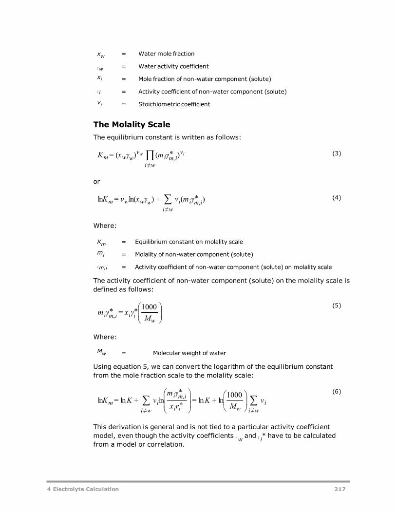
xw = Water mole fraction
ᵧw = Water activity coefficient
xi = Mole fraction of non-water component (solute)
ᵧ i = Activity coefficient of non-water component (solute)
vi = Stoichiometric coefficient
The Molality ScaleThe equilibrium constant is written as follows:
∏K x γ m γ= ( ) ( * )m w wv
i w
i m iv
≠,
w i (3)
or
∑K v x γ v m γln = ln( ) + ( * )m w w wi w
i i m i≠
,(4)
Where:
Km = Equilibrium constant on molality scale
mi = Molality of non-water component (solute)
ᵧm,i = Activity coefficient of non-water component (solute) on molality scale
The activity coefficient of non-water component (solute) on the molality scale isdefined as follows:
m γ x γM
* = *1000
i m i i iw
,
(5)
Where:
Mw = Molecular weight of water
Using equation 5, we can convert the logarithm of the equilibrium constantfrom the mole fraction scale to the molality scale:
∑ ∑K K vm γ
x rK
Mvln = ln + ln
*
*= ln + ln
1000m
i w
i
i m i
i i w i w
i
≠
,
≠
(6)
This derivation is general and is not tied to a particular activity coefficientmodel, even though the activity coefficients ᵧw and ᵧ i* have to be calculatedfrom a model or correlation.
4 Electrolyte Calculation 217

ExampleFor the reaction:
NaCl Na Cl↔ ++ − (7)
The equilibrium constant is:
Ka a
a=
.Na Cl
NaCl
+ − (8)
Where a is the activity of a species. Therefore, we have:
v v v= = 1, = − 1Na Cl NaCl
+ − (9)
∑ v v v v= + + = 1
i w
i Na Cl NaCl
≠
+ − (10)
K KM
ln = ln + ln1000
m
w
(11)
Equation 11 holds for all 1-1 aqueous electrolytes.
The molality scale equilibrium constant is usually expressed in the form:
K a b T c T d Tln = + ( / ) + ( × ln ) + ( × )m (12)
Combining equations 11 and 12, we can calculate the equilibrium constant ineither scale.
If chemical equilibrium constants are not available, the Aspen Physical PropertySystem estimates them from the reference state free energy of the system:
KG
RTln =
∆ *m
(13)
Applying equation 13 to 1-1 electrolyte systems using equation 11:
KG
RT Mln =
∆ *+ ln
1000
mm
w
(14)
More generally, we can rewrite equation 14 as follows:
∑KG
RT Mvln =
∆ *+ ln
1000m
m
w i w
i
≠
(15)
The Aspen Physical Property System offers a number of methods for calculatingG∆ *m , including Electrolyte NRTL.
218 4 Electrolyte Calculation

Electrolyte ThermodynamicModelsIn electrolyte process calculation, the following thermophysical properties mustbe computed at a given temperature, pressure and composition:
l Activity coefficientl Enthalpyl Reference state Gibbs energy
These properties are necessary to perform phase equilibrium, chemical equi-librium, and mass and energy balance calculations. Activity coefficients are themost critical properties for process calculation. They determine the flow rates,compositions, and stability of phases.
Advances in electrolyte thermodynamics have produced several semi-empiricalexcess Gibbs energy models that correlate and predict: activity coefficients ofindividual ions, mean ionic activity coefficients, and activity coefficients ofmolecular solvents and solutes. The Pitzer equation, the Electrolyte NRTLModel, and the Zemaitis equations are the most widely adopted equationsamong these models.
Pitzer EquationThe Pitzer equation is a virial expansion equation. The model requires second-order parameters at low concentrations, and both second- and third-order para-meters at high concentrations. The equation has been applied successfully torepresent data within experimental error from dilute solutions up to an ionicstrength of six molal for both aqueous single strong electrolyte systems andmulticomponent strong electrolyte systems (Pitzer, 1973). The Pitzer equationis also extended to model aqueous weak electrolyte systems (Chen et al.,1982). It provides a thermodynamically consistent model that accurately rep-resents electrolyte nonideality for many industrial aqueous electrolyte sys-tems.
This model is the basis for the PITZER property method. For details on themodel, see Pitzer Activity Coefficient Model in Physical Property Models.
ReferencesC.C. Chen, H.I. Britt, J.F Boston, and L.B. Evans, "Local Composition Model forExcess Gibbs Energy of Electrolyte Systems," AIChE J., Vol. 28, (1982), p. 588.
Pitzer, K.S., "Thermodynamics of Electrolytes.I. Theoretical Basis and GeneralEquations," J. Phys. Chem., Vol. 77, (1973), p. 268.
4 Electrolyte Calculation 219

Electrolyte NRTL EquationThe electrolyte NRTL equation provides another thermodynamically consistentmodel for aqueous electrolyte systems. This equation was developed with thelocal composition concept. This concept is similar to the NRTL (Non-RandomTwo Liquid) model for nonelectrolyte systems (Renon and Prausnitz, 1968).With only binary parameters, the equation satisfactorily represents physicalinteractions of true species in aqueous single electrolyte systems and mul-ticomponent electrolyte systems over wide ranges of concentrations and tem-peratures. This model can represent infinitely dilute electrolyte systems (whereit reduces to the Debye-Hückel model), nonelectrolyte systems (where itreduces to the NRTL model), and pure fused salts. It connects these limiting sys-tems. The equation has been extended to model mixed solvent electrolyte-sys-tems (Mock et al., 1984).
This model is the basis for the ELECNRTL property method. For details on themodel, see Electrolyte NRTL Activity Coefficient Model in Physical PropertyModels.
ReferencesB. Mock, L.B. Evans, and C.-C. Chen, "Phase Equilibria in Multiple-Solvent Elec-trolyte Systems: A New Thermodynamic Model," Paper presented at the BostonSummer Computer Simulation Conference, July 1984.
H. Renon and J.M. Prausnitz, "Local Compositions in Thermodynamic ExcessFunction for Liquid Mixtures," AIChE J., Vol. 14, (1968), p. 135.
Zemaitis Equation (Bromley-Pitzer Model)The Zemaitis equation is based on the Bronsted-Guggenheim mean ionic activ-ity coefficient equation with the Guggenheim β term expressed in Bromley'sform as an expansion of ionic strength. The activity of solvent water in singleelectrolyte systems is then computed by application of the Gibbs-Duhem integ-ration on the mean ionic activity coefficient equation. In multicomponent elec-trolyte systems, the activity coefficient of solvent water is computed with theMeissner approximation to avoid excessive Gibbs-Duhem integration (Bromley,1973). Activity coefficients of molecular solutes are estimated with theSetschenow equation. The Zemaitis equation is not a thermodynamically con-sistent model, and binary parameters are empirical functions of ionic strength.The model offers the advantage of predicting mean ionic activity coefficientsfor unmeasured electrolyte systems from Bromley's correlation of binary para-meters (Meissner and Kusik, 1973). For details on the model, see Bromley-Pitzer Activity Coefficient Model in Physical Property Models.
ReferencesL.A. Bromley, "Thermodynamic Properties of Strong Electrolytes in AqueousSolutions," AIChE J., Vol. 18, (1973), p. 313.
220 4 Electrolyte Calculation

H.P. Meissner and C.L. Kusik, "Aqueous Solutions of Two or More Strong Elec-trolytes-Vapor Pressures and Solubilities," Ind. Eng. Chem. Process Res.Develop., Vol. 12, (1973), p. 205.
Electrolyte Data RegressionData regression is a critical part of electrolyte process calculation. Forexample, electrolyte activity coefficient models require regression of exper-imental data to determine model parameters. It may also be necessary todetermine chemical equilibrium constants by data regression.
The Aspen Physical Property System Data Regression System (DRS) can beused for electrolytes. There are two unique considerations for electrolyte sys-tems:
l Ions are nonvolatile, so vapor-liquid phase equilibrium constraints forions are not applicable.
l The chemical equilibrium constraint of the solution chemistry must besatisfied.
Experimental data for electrolyte systems can be divided into four main cat-egories for both single electrolyte systems and multicomponent electrolyte sys-tems:
l Electrolyte properties, such as mean ionic coefficientsl Molecular properties, such as osmotic coefficient, solvent vapor pres-sure, vapor-liquid phase equilibrium data, and liquid-liquid phase equi-librium data
l Solution properties, such as liquid mixture enthalpy and densityl Salt solubility
Electrolyte data regression is most often performed on electrolyte propertiesand molecular properties to determine activity coefficient model parameters.Solution enthalpy data provide valuable information on temperature derivativesof activity coefficients and can be used with other data to determine the tem-perature dependency of activity coefficient model parameters. These data canalso be used to regress chemical equilibrium constants and activity coefficientmodel parameters. Salt saturation limits can be used to obtain equilibrium con-stants for salt precipitation (salt solubility product).
See Regressing Property Data in Using the Properties Environment in help fordetails on data regression.
4 Electrolyte Calculation 221

222 4 Electrolyte Calculation

5 Free-Water and RigorousThree-Phase Calculations
This chapter describes free-water, dirty-water, and rigorous three-phase cal-culations in the Aspen Physical Property System. Guidelines to help you choosethe most appropriate method are included.
The following table lists the unit operation models that allow three-phase cal-culations. The table shows, for each model, whether or not free-water, dirty-water, and/or rigorous three-phase calculations can be performed.
Unit Operation Models That Allow Three-Phase Calculations
Name Description Free-WaterCalculations
Dirty-WaterCalculations
WaterDecantStream
Rigorous3-Phase Cal-culations
Mixer Stream mixer YES YES YES YES
FSplit Stream splitter YES YES NO YES
Sep Component separator YES YES NO YES
Sep2 Two outlet separator YES YES NO YES
DSTWU Shortcut distillationdesign
YES † YES † YES NO
Distl Shortcut distillation rat-ing
YES † YES † YES NO
SCFrac Shortcut petroleum dis-tillation
YES † NO YES NO
RadFrac Rigorous distillation YES YES YES YES
MultiFrac Rigorous multicolumn dis-tillation
YES NO YES NO
5 Free-Water and Rigorous Three-Phase Calculations 223

Name Description Free-WaterCalculations
Dirty-WaterCalculations
WaterDecantStream
Rigorous3-Phase Cal-culations
PetroFrac Rigorous petroleum dis-tillation
YES NO YES NO
Extract Rigorous liquid-liquidextractor
NO NO NO ††
Heater Heater/cooler YES YES YES YES
Flash2 Two outlet flash YES YES YES YES
Flash3 Three outlet flash NO NO NO YES
Decanter Liquid-liquid decanter YES NO NO ††
Heatx Two stream heatexchanger
YES YES YES YES
MHeatx Multistream heatexchanger
YES YES YES YES
RStoic Stoichiometric reactor YES YES YES YES
RYield Yield reactor YES YES YES YES
RGibbs Equilibrium reactorGibbs energy min-imization
NO NO NO YES †††
Pump Pump/hydraulic turbine YES YES YES YES
Compr Compressor/turbine YES YES YES YES
MCompr Multistage com-pressor/turbine
YES YES YES YES
Crystallizer Crystallizer NO NO NO NO
Pipeline Pipeline YES NO NO YES
Dupl Stream duplicator — — — —
Mult Stream multiplier — — — —
†Condenser only
††Rigorous liquid-liquid equilibrium calculations
†††RGibbs handles any number of phases rigorously.
Free-Water and Dirty-WaterImmiscibility Simplification
224 5 Free-Water and Rigorous Three-Phase Calculations

The unit operation models in the table labeled Unit Operation Models That AllowThree-Phase Calculations can handle the presence and the decanting of freewater or dirty water, when performing flash calculations or liquid-liquid equi-librium calculations on water-organic systems in which the water phase isessentially pure or has trace amounts of organic components.
Free-water calculations involve special methods for calculating the solubility ofwater in the organic phase and a test for the presence of a pure water phase.Free-water calculations are always faster than rigorous three-phase cal-culations and require minimal physical property data preparation. Just likefree-water calculations, dirty-water calculations also involve special methodsfor calculating the solubility of water in the organic phase. In addition to this,special methods are used to compute the aolubility of organic compounds in thewater phase.
For water-hydrocarbon systems, free-water calculations are normallyadequate. The hydrocarbon solubility in the water phase is generally negligible.In applications where the hydrocarbon solubility in the water phase is of greatconcern (such as in an environmental study), use dirty-water or rigorous three-phase calculations.
For chemical systems such as water-higher alcohols, free-water or dirty-watercalculations do not apply. Solubility of the organics in the water phase is sig-nificant. Rigorous three-phase calculations are required.
When you use the free-water or dirty-water calculation method, if a stream con-tains only water, all properties for the stream are calculated using the free-water method as if it was the main property method.
Specifying Free-Water or Dirty-Water Cal-culationsThe free-water or dirty-water calculations are completely rigorous, except forthe assumption that the water phase is pure or has only a trace amount oforganic components. If free water or dirty water is present and you specify adecant stream for the block, the Aspen Physical Property System places thewater phase in the decant stream. If you do not specify a decant stream, theAspen Physical Property System mixes the water phase with the organic phase.
To request free-water or dirty-watercalculations for
Use the Free-Water field to Yes orDirty on the
The entire flowsheet Setup Specifications Global sheet
An individual unit operation block Block Options form for the block
An individual outlet stream in some blocks Flash-Specs form for the block
For all unit operation blocks except the distillation models, you can select twotypes of free-water calculations using the following flash specification:
5 Free-Water and Rigorous Three-Phase Calculations 225
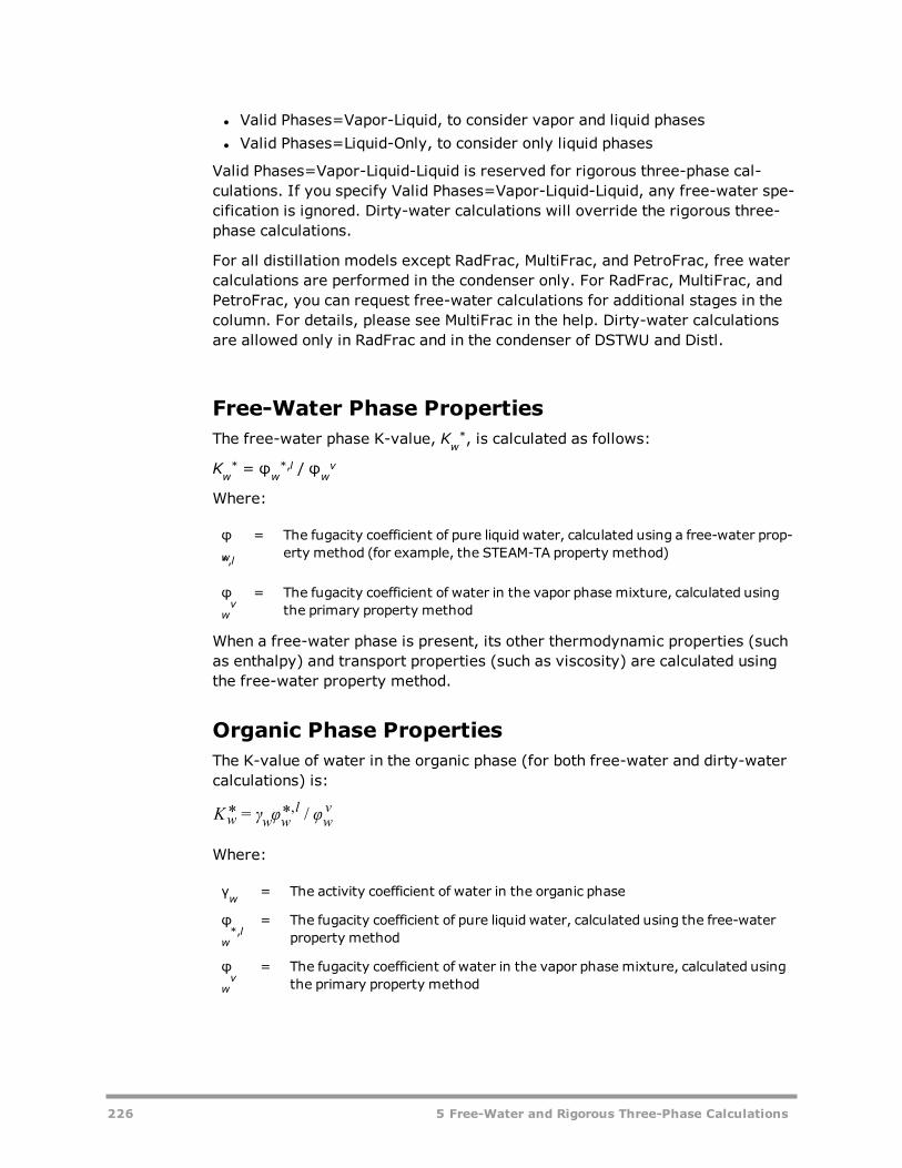
l Valid Phases=Vapor-Liquid, to consider vapor and liquid phasesl Valid Phases=Liquid-Only, to consider only liquid phases
Valid Phases=Vapor-Liquid-Liquid is reserved for rigorous three-phase cal-culations. If you specify Valid Phases=Vapor-Liquid-Liquid, any free-water spe-cification is ignored. Dirty-water calculations will override the rigorous three-phase calculations.
For all distillation models except RadFrac, MultiFrac, and PetroFrac, free watercalculations are performed in the condenser only. For RadFrac, MultiFrac, andPetroFrac, you can request free-water calculations for additional stages in thecolumn. For details, please see MultiFrac in the help. Dirty-water calculationsare allowed only in RadFrac and in the condenser of DSTWU and Distl.
Free-Water Phase PropertiesThe free-water phase K-value, Kw
*, is calculated as follows:
Kw* = φw
*,l / φwv
Where:
φw*,l
= The fugacity coefficient of pure liquid water, calculated using a free-water prop-erty method (for example, the STEAM-TA property method)
φwv
= The fugacity coefficient of water in the vapor phase mixture, calculated usingthe primary property method
When a free-water phase is present, its other thermodynamic properties (suchas enthalpy) and transport properties (such as viscosity) are calculated usingthe free-water property method.
Organic Phase PropertiesThe K-value of water in the organic phase (for both free-water and dirty-watercalculations) is:
K γ φ φ* = * /w w wl
wv,
Where:
γw = The activity coefficient of water in the organic phase
φw*,l
= The fugacity coefficient of pure liquid water, calculated using the free-waterproperty method
φwv
= The fugacity coefficient of water in the vapor phase mixture, calculated usingthe primary property method
226 5 Free-Water and Rigorous Three-Phase Calculations
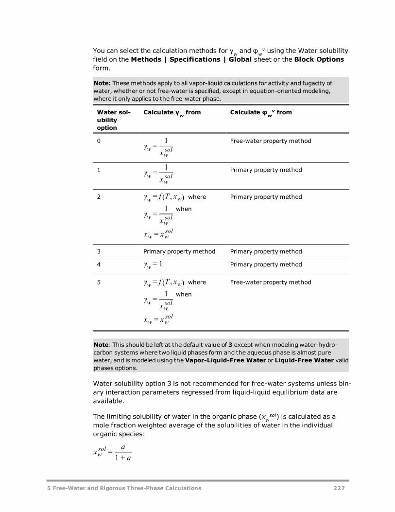
You can select the calculation methods for γw and φwv using the Water solubility
field on the Methods | Specifications | Global sheet or the Block Optionsform.
Note: These methods apply to all vapor-liquid calculations for activity and fugacity ofwater, whether or not free-water is specified, except in equation-orientedmodeling,where it only applies to the free-water phase.
Water sol-ubilityoption
Calculate γw from Calculate φwv from
0γ
x=1
wwsol
Free-water property method
1 γx
=1
wwsol
Primary property method
2 γ f T x= ( , )w w where
γx
=1
wwsol
when
x x=w wsol
Primary property method
3 Primary property method Primary property method
4 γ = 1w Primary property method
5 γ f T x= ( , )w w where
γx
=1
wwsol
when
x x=w wsol
Free-water property method
Note: This should be left at the default value of 3 except when modeling water-hydro-carbon systems where two liquid phases form and the aqueous phase is almost purewater, and is modeled using the Vapor-Liquid-Free Water or Liquid-Free Water validphases options.
Water solubility option 3 is not recommended for free-water systems unless bin-ary interaction parameters regressed from liquid-liquid equilibrium data areavailable.
The limiting solubility of water in the organic phase (xwsol) is calculated as a
mole fraction weighted average of the solubilities of water in the individualorganic species:
xa
a=1 +
wsol
5 Free-Water and Rigorous Three-Phase Calculations 227

∑a xx
x=
1 −i
iwisol
wisol
Where:
xi = Water-free mole fraction of the ith organic species
xwisol = Mole fraction solubility of water in the ith species
The value of xwisol is calculated as a function of temperature, using the Water
Solubility model (WATSOL).
Dirty-Water Phase Properties
The K-value of water in the dirty-water phase, K*w , is calculated as follows:
K φ φ* = * /w wl
wv,
Where:
φw*,l
= The fugacity coefficient of pure liquid water, calculated using a free-waterproperty method (for example, the STEAM-TA property method)
φwv
= The fugacity coefficient of water in the vapor phase mixture, calculated usingthe primary property method
The K-values of other components are calculated as follows:
Kγ φ
φ=i
i il
iv
Where:
γx
=1
iisol
xisol, the solubility of component i in water, is calculated using the Hydrocarbon
Solubility model (HCSOL).
Rigorous Three-Phase CalculationsThe unit operation models that can perform rigorous three-phase or two-liquid-phase calculations are indicated in the table labeled Unit Operation Models ThatAllow Three-Phase Calculations. These calculations make no assumptions aboutthe nature of the two liquid phases. The Aspen Physical Property System usesthe primary property method to calculate the K-values of all components inboth liquid phases. The second liquid phase does not have to be aqueous. If thesecond liquid phase is aqueous, the solubility of organics in water is treated
228 5 Free-Water and Rigorous Three-Phase Calculations

rigorously. To obtain correct three-phase results, you must use the appropriatebinary parameters for the property model used in the property method.
Specify rigorous three-phase calculations at the individual block level, using theflash option Valid Phases=Vapor-Liquid-Liquid, except for Flash3. Flash3 has noflash options, since it performs only rigorous three-phase flashes.
Extract always performs rigorous two-liquid-phase calculations.
5 Free-Water and Rigorous Three-Phase Calculations 229

230 5 Free-Water and Rigorous Three-Phase Calculations

6 Petroleum ComponentsCharacterization Methods
The Aspen Physical Property System provides a wide range of methods for char-acterization of petroleum fractions, or pseudocomponents. These methods areused to estimate parameters, such as critical temperature, and properties,such as ideal gas heat capacity, vapor pressure, and liquid viscosity. The fol-lowing table lists the:
l Parameters that the Aspen Physical Property System estimates for pet-roleum fractions
l Methods available for each parameter. The literature references for eachmethod are listed at the end of this chapter.
Petroleum Fractions Characterization Methods
Parameter Description Methods Available
MW Molecular weight Brule et al. (1982)Extended API (2002)Extended Twu (2002)Hariu-Sage (1969)Hariu-Sage-Aspen (1994)Kesler-Lee (1976)Riazi API (1986)Riazi API (1986), heavy petroRiazi-Daubert (1980)Tsang-Aspen (1978)User routine PCMWUWinn correlation (1957)
6 Petroleum Components Characterization Methods 231

Parameter Description Methods Available
TC Critical temperature Brule et al. (1982)Cavett (1962)Extended Twu 1 (2002)Extended Twu 2 (2002)Extended Cavett (2002)Kesler-Lee (1976)Riazi API (1986)Riazi-Daubert (1980)Robinson-Peng (1978)Tsang-Aspen (1978)Twu (1984)User routine PCTCUWinn correlation (1957)
PC Critical pressure Cavett (1962)Extended Edmister (2002)Extended Twu(2002)Kesler-Lee (1976)Riazi API (1986)Riazi-Daubert (1980)Robinson-Peng (1978)Tsang-Aspen (1978)Twu (1984)User routine PCPCUWinn correlation (1957)
VC Critical volume Brule et al. (1982)Edmister (1984)Extended Twu (2002)Lee-Kesler (1984)Riedel (1954)Twu (1984)User routine PCVCU
OMEGA Acentric factor Defining relationEdmister (1984)Extended Lee-Kesler (2002)Kesler-Lee (1976)Kesler-Lee-Aspen (1994)Robinson-Peng (1978)User routine PCOMGUTwu generalized correlation (1994)Aspen-Twu generalized correlation
PL Vapor pressure BK-10 (AspenTech implementation)Kesler-Lee (1980)Maxwell-Bonnell (1955)Tsang-SWAP (1978)User routine PCPLU
232 6 Petroleum Components Characterization Methods

Parameter Description Methods Available
VL Liquidmolar volume Cavett (1974)Rackett (Spencer and Danner, 1972)User routine PCVOLU
WATSOL Water solubility inhydrocarbon
AspenAPI KeroseneHibbard-Schalla (API)User routine PCWSLUUser routine PCWSLU2
HCSOL Hydrocarbon sol-ubility in water-richphase
AspenUser routine PCHSLU
MUL Liquid viscosity Watson (1935)User routine PCMULUUser routine PCMULU2
CPIG Ideal gas heat capa-city
API HybridBrule et al. (1982)Cavett (1962)Kesler-Lee (1976)Mathias-Monks (1982)Simplified Lee-KeslerTsang-Aspen (1978)User routine PCCPGU
DHVL Enthalpy of vapor-ization
Kistiakowsky (1923)Vetere (1973)User routine PCDHVU
DHFORM Ideal gas heat offormation at 298.15K
Default to zeroEdmister (1988) ††Edmister-API (1988) ††Edmister-API97 (1988) ††User routine PCDHFU
DGFORM Ideal gas Gibbs freeenergy of formationat 298.15 K
Default to zeroEdmister (1988) ††Edmister-API97 (1988) ††User routine PCDGFU
RKSKBV RKS binary inter-action parameters †
API 1978API 1987User routine PCRKIUUser routine PCRKIU2
BWRGMA BWR orientation para-meter
Brule et al. (1982)User routine PCBWRU
6 Petroleum Components Characterization Methods 233

Parameter Description Methods Available
TCBWR BWR critical tem-perature
Brule et al. (1982)User routine PCBWRU
VCBWR BWR critical volume Brule et al. (1982)User routine PCBWRU
† The RKS binary interaction parameters are estimated for each pseudo-component in pairs with certain light gases which are present in the simulation.The 1978 method estimates parameters for pseudocomponents with CO2, CO,H2S, N2. The 1987 method estimates parameters for pseudocomponents withmethane, CO2, H2S, N2, and H2, and sets the parameters for pseudocomponentswith CO to zero.
†† The Edmister methods use data for paraffin, naphthene, and aromatic con-tent (sometimes called PNA analysis), but the implementations in the AspenPhysical Property System use an API correlation based on molecular weight,refractive index, liquid density, liquid viscosity, and specific gravity to determ-ine these values, even if you have entered values for these properties of thepseudocomponents.
AspenTech Extensions to Char-acterization Methods for Pet-roleum FractionsA number of the methods for characterization of petroleum fractions areAspenTech extensions to well-known methods. These are listed below. Plots areavailable showing how some of the extended methods compare for a typicalcrude assay.
Property Method Description
Molecularweight
Hariu andSage-Aspen
Hariu-Sage (1969)model with Aspen modification forlight fractions.
Extended API Riazi-Daubert (1980)model with Aspen modificationfor light fractions.
Extended Twu Twu (1984)model with Aspen modification for high-boiling fractions.
Critical tem-perature
Extended Twu1
Twu (1984)model with Aspen modification for high-boiling fractions using linear extrapolation.
234 6 Petroleum Components Characterization Methods

Property Method Description
Extended Twu1
Twu (1984)model with Aspen modification for high-boiling fractions using extrapolation based on constantWatson K.
ExtendedCavett
Cavett (1962)model with Aspen modification forhigh-boiling fractions.
Critical pres-sure
ExtendedEdmister
Edmister (1984)model with Aspen modification forhigh-boiling fractions.
Extended Twu Twu (1984)model with Aspen modification for high-boiling fractions.
Criticalvolume
Extended Twu Twu (1984)model with Aspen modification for high-boiling fractions.
Acentricfactor
Lee andKesler, Aspen
Kesler-Lee (1976)model with Aspen modification forhigh-boiling fractions.
Extended Lee-Kesler
Further modifications for high-boiling fractions.
Aspen-Twugeneralizedcorrelation
Twu generalized correlation (1994) with Aspenimprovement for heavy components.
Water sol-ubility
Aspen AspenTech empirical correlation
Ideal gasheat capa-city
API Hybrid Combination of API Technical databook procedure7D4.2 and Brule et al. (1982)
Simplified Lee-Kesler
Kesler-Lee (1976)model with AspenTech modi-fication.
6 Petroleum Components Characterization Methods 235

Comparison of Extended Molecular WeightMethods
Comparison of Extended Critical Tem-perature Methods
236 6 Petroleum Components Characterization Methods

Comparison of Extended Critical PressureMethods
6 Petroleum Components Characterization Methods 237
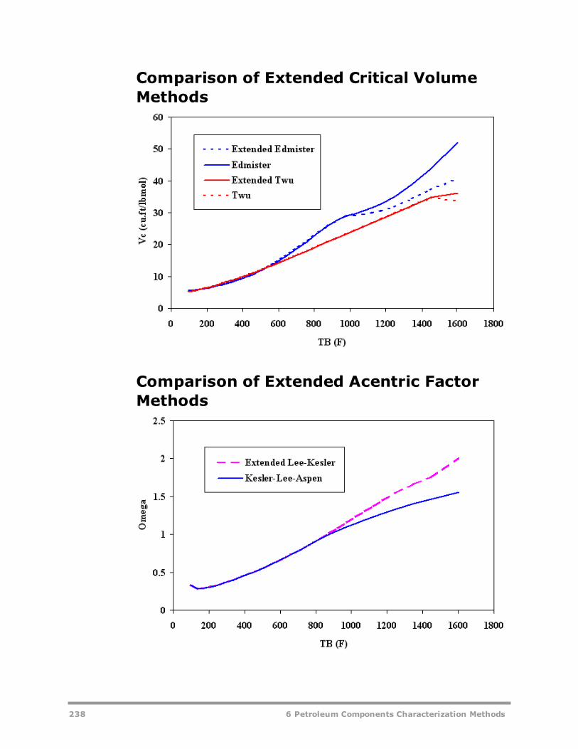
Comparison of Extended Critical VolumeMethods
Comparison of Extended Acentric FactorMethods
238 6 Petroleum Components Characterization Methods

User Models for Char-acterization of Petroleum Frac-tionsAll characterization parameters and properties of petroleum fractions can beestimated by user routines. See Aspen Plus User Models, Chapter 25, for detailson writing these routines.
Property Routine
Molecular weight PCMWU
Critical temperature PCTCU
Critical pressure PCPCU
Critical volume PCVCU
Acentric factor PCOMGU
Vapor pressure PCPLU
Liquidmolar volume PCVOLU
Water solubility PCWSLU, PCWSLU2
Hydrocarbon solubility PCHSLU
Liquid viscosity PCMULU, PCMULU2
Ideal gas heat capacity PCCPGU
Enthalpy of vaporization PCDHVU
Standard enthalpy of formation PCDHFU
Standard Gibbs free energy of formation PCDGFU
RKS interaction parameters PCRKIU, PCRKIU2
BWR orientation parameter, Tc, Vc PCBWRU
Normal boiling point PCABPU
Specific gravity PCSGU
6 Petroleum Components Characterization Methods 239

Property Methods for Char-acterization of Petroleum Frac-tionsSince there are several methods available for estimation of a given parameter,it is often difficult to select the appropriate method for the application. For yourconvenience, we have grouped several sets of methods into property methods.These selections are made according to standard industry practices, most com-monly used methods, or based on AspenTech's own extensions. The AspenTechextensions are intended to improve the behavior of the correlations in the lowand high-boiling ranges.
The following property methods are available:
l The API-METH property method consists of methods based mainly on theAPI procedure. This property method is appropriate for refinery applic-ations.
l COAL-LIQ property method consists of methods developed for coal liquidapplications. The database used to develop the correlations contains alarge percentage of aromatic compounds.
l ASPEN property method consists of methods developed by AspenTechfor petroleum components and methods based on the API procedure.This method is recommended.
l LK property method is based mainly on the methods of Kesler and Lee.l API-TWU property method is based on the ASPEN property method, butuses the Twu correlations for critical properties.
l EXT-TWU property method is similar to the API-TWU method, exceptthat AspenTech extensions to both low boiling and high boiling rangesare used for MW, TC, PC, VC, and acentric factor.
l EXT-API property method is similar to the EXT-TWU method, except thatthe extended API method is used for molecular weight and the extendedLee-Kesler method is used for acentric factor.
l EXT-CAV property method is similar to the EXT-API method, except thatthe extended Cavett method is used for critical temperature and theextended Edmister method is used for critical pressure and criticalvolume.
There are no documented temperature limits for these methods from theirauthors, but our studies show that the limits within which the methods are reli-able depend on the property. The first five methods typically behave properlyfor fractions up to a normal boiling point of 800 to 1000 F. The extended meth-ods extend the range of applicability for MW, TC, PC, and acentric factor to anormal boiling point of about 1500 F.
240 6 Petroleum Components Characterization Methods

The models associated with each of the property methods available for char-acterization of pseudocomponents are listed in the tables below.
Property Method ASPEN: Aspen Tech andAPI procedures
Property Model
Molecular weight Hariu and Sage-Aspen
Tc Riazi-Daubert
Pc Riazi-Daubert
Vc Riedel
Acentric factor Lee and Kesler, Aspen
Vapor pressure BK-10
Liquidmolar volume Rackett
Water solubility Aspen
Liquid viscosity Watson
Ideal gas heat capacity Kesler-Lee
Enthalpy of vaporization Vetere
Standard enthalpy of formation Edmister
Standard Gibbs energy of formation Edmister
RKS binary parameters API 1978
Property Method API-METH: API Pro-cedures
Property Model
Molecular weight Hariu-Sage
Tc Riazi-Daubert
Pc Riazi-Daubert
Vc Riedel
Acentric factor Kesler-Lee
Vapor pressure Maxwell-Bonnell
6 Petroleum Components Characterization Methods 241

Property Model
Liquidmolar volume Rackett
Water solubility Aspen
Liquid viscosity Watson
Ideal gas heat capacity Kesler-Lee
Enthalpy of vaporization Vetere
Standard enthalpy of formation Default to zero
Standard Gibbs energy of formation Default to zero
RKS binary parameters API 1978
BWR orientation parameter, Tc, Vc Brule et al.
Property Method COAL-LIQ: for CoalLiquids
Property Model
Molecular weight Hariu-Sage
Tc Tsang-Aspen
Pc Tsang-Aspen
Vc Riedel
Acentric factor Kesler-Lee
Vapor pressure Tsang-SWAP
Liquidmolar volume Rackett
Water solubility Aspen
Liquid viscosity Watson
Ideal gas heat capacity Mathias-Monks
Enthalpy of vaporization Vetere
Standard enthalpy of formation Default to zero
Standard Gibbs energy of formation Default to zero
RKS binary parameters API 1978
BWR orientation parameter, Tc, Vc Brule et al.
242 6 Petroleum Components Characterization Methods

Property Method LK: Lee-Kesler
Property Model
Molecular weight Kesler-Lee
Tc Kesler-Lee
Pc Kesler-Lee
Vc Riedel
Acentric factor Kesler-Lee
Vapor pressure Kesler-Lee
Liquidmolar volume Rackett
Water solubility Aspen
Liquid viscosity Watson
Ideal gas heat capacity Kesler-Lee
Enthalpy of vaporization Vetere
Standard enthalpy of formation Edmister
Standard Gibbs energy of formation Edmister
RKS binary parameters API 1978
Property Method API-TWU: AspenTech,API, and Twu
Property Model
Molecular weight Hariu and Sage-Aspen
Tc Twu
Pc Twu
Vc Twu
Acentric factor Lee and Kesler, Aspen
Vapor pressure BK-10
Liquidmolar volume Rackett
Water solubility API kerosene-line
Liquid viscosity Watson
6 Petroleum Components Characterization Methods 243

Property Model
Ideal gas heat capacity Kesler-Lee
Enthalpy of vaporization Vetere
Standard enthalpy of formation Edmister
Standard Gibbs energy of formation Edmister
RKS binary parameters API 1978
Property Method EXT-TWU: Twu andAspenTech Extensions
Property Model
Molecular weight Extended Twu
Tc Extended Twu
Pc Extended Twu
Vc Extended Twu
Acentric factor Extended Twu
Vapor pressure BK-10
Liquidmolar volume Rackett
Water solubility API kerosene-line
Liquid viscosity Watson
Ideal gas heat capacity Kesler-Lee
Enthalpy of vaporization Vetere
Standard enthalpy of formation Edmister
Standard Gibbs energy of formation Edmister
RKS binary parameters API 1978
Property Method EXT-API: API, Twu, andAspenTech Extensions
Property Model
Molecular weight Extended API correlation
244 6 Petroleum Components Characterization Methods

Property Model
Tc Extended Twu
Pc Extended Twu
Vc Extended Twu
Acentric factor Extended Lee-Kesler
Vapor pressure BK-10
Liquidmolar volume Rackett
Water solubility API kerosene-line
Liquid viscosity Watson
Ideal gas heat capacity Kesler-Lee
Enthalpy of vaporization Vetere
Standard enthalpy of formation Edmister
Standard Gibbs energy of formation Edmister
RKS binary parameters API 1978
Property Method EXT-CAV: Cavett, API, andAspenTech Extensions
Property Model
Molecular weight Extended API correlation
Tc Extended Cavett
Pc Extended Edmister
Vc Extended Edmister
Acentric factor Extended Lee-Kesler
Vapor pressure BK-10
Liquidmolar volume Rackett
Water solubility Aspen
Liquid viscosity Watson
Ideal gas heat capacity Kesler-Lee
Enthalpy of vaporization Vetere
Standard enthalpy of formation Edmister
6 Petroleum Components Characterization Methods 245
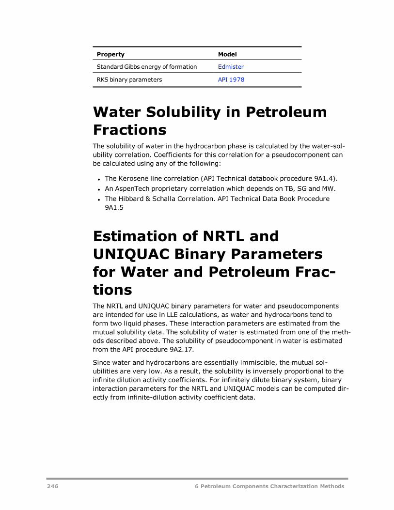
Property Model
Standard Gibbs energy of formation Edmister
RKS binary parameters API 1978
Water Solubility in PetroleumFractionsThe solubility of water in the hydrocarbon phase is calculated by the water-sol-ubility correlation. Coefficients for this correlation for a pseudocomponent canbe calculated using any of the following:
l The Kerosene line correlation (API Technical databook procedure 9A1.4).l An AspenTech proprietary correlation which depends on TB, SG and MW.l The Hibbard & Schalla Correlation. API Technical Data Book Procedure9A1.5
Estimation of NRTL andUNIQUAC Binary Parametersfor Water and Petroleum Frac-tionsThe NRTL and UNIQUAC binary parameters for water and pseudocomponentsare intended for use in LLE calculations, as water and hydrocarbons tend toform two liquid phases. These interaction parameters are estimated from themutual solubility data. The solubility of water is estimated from one of the meth-ods described above. The solubility of pseudocomponent in water is estimatedfrom the API procedure 9A2.17.
Since water and hydrocarbons are essentially immiscible, the mutual sol-ubilities are very low. As a result, the solubility is inversely proportional to theinfinite dilution activity coefficients. For infinitely dilute binary system, binaryinteraction parameters for the NRTL and UNIQUAC models can be computed dir-ectly from infinite-dilution activity coefficient data.
246 6 Petroleum Components Characterization Methods

Estimation of ATOMNO andNOATOM for Petroleum Frac-tionsATOMNO and NOATOM, which combine to form the chemical formula, are estim-ated from the molecular weight and carbon-to-hydrogen (C/H) ratio. The C/Hratio is estimated using the procedure in Technical Data Book - Petroleum Refin-ing, vol. 2, fig. 2B6.1, American Petroleum Institute, 1983. These componentsare assumed to contain no atoms but carbon and hydrogen, and the carbon andhydrogen numbers are adjusted to meet the molecular weight and C/H ratio. Asa result, H and C may be fractional.
Estimation of Flash PointAspen Plus provides several properties representing different methods of cal-culating the flash point. The following methods are available:
l FLPT-API, the API method for determining flash pointl FLPT-PM, the Pennsky-Martens method (ASTM-D93)l FLPT-TAG, the Tag method (ASTM-D56)
FLPT-API uses the ASTM D86 10% temperature for the petroleum fraction orthe normal boiling point for pure components in a procedure based on the APIcomputerized procedure 2B7.1 (Riazi, 1985, 1986). Linear extrapolation is alsoperformed. The following correlation is used:
TFPa b T R c T R
=1
− + / 10 + ln( 10 )
Where
TFP = Flash point temperature in Rankine
T10R = D86 temperature at 10% volume, in Rankine
a, b, c = constants
The other two methods use a modified bubble point calculation described inSeader and Henley (1998). These methods use mole-weight-modified K-values
for a bubble point flash in which the value of the summation∑ K Xi i , normally1, has been replaced with an experimentally determined parameter a. The para-meter a has different values for the two methods.
6 Petroleum Components Characterization Methods 247

Petroleum Method References(BK10) AspenTech implementation of the method described in B.C. Cajander etal., Prediction of Equilibrium Ratios from Nomograms of Improved Accuracy,"J. Chem. Eng. Data, 5 (3), p. 251 (1960), and in J.M. Lenoir, "Predict K Valuesat Low Temperatures," Hydro. Proc., (1969).
Brulé, M.R., C.T. Lin, L.L. Lee, and K.E. Starling, AIChE J., 28, p. 616 (1982).
Cavett, R.H., "Physical Data for Distillation Calculations – Vapor-Liquid Equi-libria," Presented at 27th Midyear Meeting of API Division of Refining, May 15,1962.
Cavett, R.H., FLOWTRAN Physical Properties Reference Manual, Monsanto Com-pany, 1974.
Edmister, W.C. and B.I. Lee, Applied Hydrocarbon Thermodynamics, 2nd edi-tion, Vol. 1, Ch. 7, Gulf Publishing Co., (1988).
Edmister, W.C., Applied Hydrocarbon Thermodynamics, 2nd edition, Vol. 2, Ch.24, Gulf Publishing Co., (1988). Used for Edmister and Edmister-API97 meth-ods. The Edmister-API97 methods use the API97 viscosity model instead of theolder API model.
Edmister, W.C., Applied Hydrocarbon Thermodynamics, 2nd edition, Vol. 2, Ch.25, Gulf Publishing Co., (1988). Used for Edmister-API method.
Hariu, O.H. and R.C. Sage, Hydro. Proc., (1969).
Hibbard and Schalla, Water solubility parameters from API Databook procedure9A1.5; Natl. Advisory Comm. Aeron. Rm. E52024 (1952).
Kerosene line from API Databook, Figure 9A1.4.
Kesler, M.G. and B.I. Lee, Hydro. Proc., 55 (3), p. 153, (1976).
Kesler, M.G. and B.I. Lee, Hydro. Proc., 59 (7), p. 163, (1980).
Kistiakowsky, W., Z. Phys. Chem., 107, 65 (1923).
Mathias, P.M., and K.G. Monks, SRC-I Quarterly Progress Report, Air Productsand Chemicals, Inc., April – June 1982.
Maxwell and Bonnell, API Procedure 5A1.15 (1955).
Redlich-Kwong-Soave interaction parameters from API Databook, Table 8D1.3,3rd Ed (1978).
Redlich-Kwong-Soave interaction parameters from API Databook, Table 8D1.3,5th Ed (1987).
Riazi, M.R., private communication, 1985. and M.R. Riazi, API Databook, 5thEd., procedure 2B7.1 (1986).
Riazi, M.R., API Databook, 5th Ed., 2B2.B (1986). Model for heavy petroleumfractions for a molecular weight range of 200-800.
248 6 Petroleum Components Characterization Methods

Riazi, M.R., API Databook, 5th Ed., 4D3.1 (1986).
Riazi, M.R. and T.E. Daubert, Hydro. Proc., 59 (3), p. 115, (1980).
Riedel, L., API Prodedure 4A3.1 (1954).
Robinson D.B., and D.Y. Peng "The Characterization of the Heptanes and Heav-ier Fractions for the GPA Peng-Robinson Programs," GPA Research Report RR-28, March (1978).
Seader, J.D. and Ernest J. Henley, Separation Process Principles, p. 281, Wileyand Sons, 1998.
Spencer, C.F. and R.P. Danner, J. Chem Eng. Data., 17, (1972).
Tsang, M., Computer-Aided Industrial Process Design, The ASPEN Project,Second Annual Report, June 1, 1977 to May 30, 1978; Submitted to U.S. D.O.E.by M.I.T. Department of Chemical Engineering and Energy Laboratory underContract No. E(49–18) 2295, Task No. 9, June 15, 1978.
Twu, C.H., "An Internally Consistent Correlation for Predicting the Critical Pro-peties and Molecular Weights of Petroleum and Coal-Tar Liquids," Fluid PhaseEquilibria, 16, p. 137 (1984).
Twu, C.H., J.E. Coon, and J.R. Cunningham, "A Generalized Vapor PressureEquation for Heavy Hydrocarbons", Fluid Phase Equilibria, 96, p. 19-31 (1994).
Vetere, A., "Modification of the Kistiakowsky Equation for the Calculation of theEnthalpies of Vaporization of Pure Compounds," Laboratory Richerche ChimicaIndustriale SNAM PROGETTI, San Donato, Milanese, 1973.
Watson, K. et al., API Figure 11A4.1 (1935).
Winn, F.W., The Petroleum Refiner, 36, p. 157, (1957).
6 Petroleum Components Characterization Methods 249

250 6 Petroleum Components Characterization Methods

7 Property Parameter Estim-ation
This chapter describes:
l Estimation methods used by the Property Constant Estimation System(PCES)
l How to generate a report for the estimated parameters
If you request estimation, the Aspen Physical Property System, by default,estimates all missing property parameters required by physical property mod-els. These parameters include any not available in the databank and not spe-cified on Properties Parameters forms. The following table labeled ParametersEstimated by the Aspen Physical Property System lists all the parameters thatthe Aspen Physical Property System can estimate.
Parameters Estimated by theAspen Physical Property Sys-temSee Physical Property Models for more information on the models listed below.
Pure Component Constants
Parameter Description Model
MW Molecular weight
TB Normal boiling point
TC Critical temperature
7 Property Parameter Estimation 251

Parameter Description Model
PC Critical pressure
VC Critical volume
ZC Critical compressibility factor
DHFORM Ideal gas heat of formation at 298.15 K
DGFORM Ideal gas Gibbs free energy of formation at298.15 K
OMEGA Pitzer acentric factor
DHVLB Heat of vaporization at TB
Pure Component Constants
Parameter Description Model
VB Liquidmolar volume at TB
VLSTD Standard liquid volume
RGYR Radius of gyration
DELTA Solubility parameter at 298.15 K
GMUQR UNIQUAC R parameter UNIQUAC
GMUQQ UNIQUACQ parameter UNIQUAC
PARC Parachor †
DHSFRM Solid enthalpy of formation at 98.15 K
DGSFRM Solid Gibbs energy of formation at 298.15 K
DHAQHG Aqueous infinite dilution enthalpy of form-ation
Helgeson
DGAQHG Aqueous infinite dilution Gibbs energy of form-ation
Helgeson
S25HG Entropy at 298.15 K Helgeson
†Parachor is needed in estimating surface tension and radius of gyration.
252 7 Property Parameter Estimation

Temperature-Dependent Property Correlation Parameters
Parameter Description Model
CPIG Ideal gas heat capacity General Pure ComponentIdeal Gas Heat Capacity
CPLDIP Liquid heat capacity General Pure ComponentLiquid Heat Capacity
CPSPO1 Solid heat capacity General Pure ComponentSolid Heat Capacity
PLXANT Vapor pressure General Pure ComponentLiquid Vapor Pressure
DHVLWT Heat of vaporization General Pure ComponentHeat of Vaporization
RKTZRA Liquidmolar volume General Pure ComponentLiquid Molar Volume
OMEGHG Helgeson OMEGA heatcapacity coefficient
Helgeson
CHGPAR Helgeson C Heat CapacityCoefficient
Helgeson
MUVDIP Vapor viscosity General Pure ComponentVapor Viscosity
MULAND Liquid viscosity General Pure ComponentLiquid Viscosity
KVDIP Vapor thermal conductivity General Pure ComponentVapor Thermal Con-ductivity
KLDIP Liquid thermal conductivity General Pure ComponentLiquid Thermal Con-ductivity
SIGDIP Surface tension General Pure ComponentLiquid Surface Tension
Binary Parameters
Parameter Description Model
WILSON/1,WILSON/2 Wilson parameters Wilson
NRTL/1, NRTL/2 NRTL parameters NRTL
UNIQ/1, UNIQ/2 UNIQUAC parameters UNIQUAC
7 Property Parameter Estimation 253
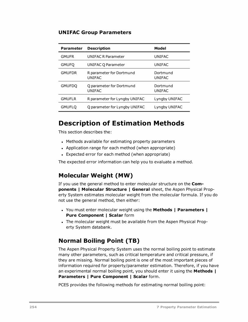
UNIFAC Group Parameters
Parameter Description Model
GMUFR UNIFAC R Parameter UNIFAC
GMUFQ UNIFAC Q Parameter UNIFAC
GMUFDR R parameter for DortmundUNIFAC
DortmundUNIFAC
GMUFDQ Q parameter for DortmundUNIFAC
DortmundUNIFAC
GMUFLR R parameter for Lyngby UNIFAC Lyngby UNIFAC
GMUFLQ Q parameter for Lyngby UNIFAC Lyngby UNIFAC
Description of Estimation MethodsThis section describes the:
l Methods available for estimating property parametersl Application range for each method (when appropriate)l Expected error for each method (when appropriate)
The expected error information can help you to evaluate a method.
Molecular Weight (MW)If you use the general method to enter molecular structure on the Com-ponents | Molecular Structure | General sheet, the Aspen Physical Prop-erty System estimates molecular weight from the molecular formula. If you donot use the general method, then either:
l You must enter molecular weight using the Methods | Parameters |Pure Component | Scalar form
l The molecular weight must be available from the Aspen Physical Prop-erty System databank.
Normal Boiling Point (TB)The Aspen Physical Property System uses the normal boiling point to estimatemany other parameters, such as critical temperature and critical pressure, ifthey are missing. Normal boiling point is one of the most important pieces ofinformation required for property/parameter estimation. Therefore, if you havean experimental normal boiling point, you should enter it using the Methods |Parameters | Pure Component | Scalar form.
PCES provides the following methods for estimating normal boiling point:
254 7 Property Parameter Estimation
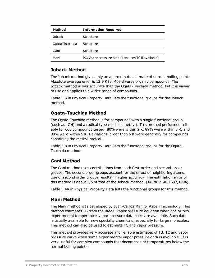
Method Information Required
Joback Structure
Ogata-Tsuchida Structure
Gani Structure
Mani PC, Vapor pressure data (also uses TC if available)
Joback MethodThe Joback method gives only an approximate estimate of normal boiling point.Absolute average error is 12.9 K for 408 diverse organic compounds. TheJoback method is less accurate than the Ogata-Tsuchida method, but it is easierto use and applies to a wider range of compounds.
Table 3.5 in Physical Property Data lists the functional groups for the Jobackmethod.
Ogata-Tsuchida MethodThe Ogata-Tsuchida method is for compounds with a single functional group(such as -OH) and a radical type (such as methyl). This method performed reli-ably for 600 compounds tested; 80% were within 2 K, 89% were within 3 K, and98% were within 5 K. Deviations larger than 5 K were generally for compoundscontaining the methyl radical.
Table 3.8 in Physical Property Data lists the functional groups for the Ogata-Tsuchida method.
Gani MethodThe Gani method uses contributions from both first-order and second-ordergroups. The second order groups account for the effect of neighboring atoms.Use of second order groups results in higher accuracy. The estimation error ofthis method is about 2/5 of that of the Joback method. (AIChE J. 40,1697,1994).
Table 3.4A in Physical Property Data lists the functional groups for this method.
Mani MethodThe Mani method was developed by Juan-Carlos Mani of Aspen Technology. Thismethod estimates TB from the Riedel vapor pressure equation when one or twoexperimental temperature-vapor pressure data pairs are available. Such datais usually available for new specialty chemicals, especially for large molecules.This method can also be used to estimate TC and vapor pressure.
This method provides very accurate and reliable estimates of TB, TC and vaporpressure curve when some experimental vapor pressure data is available. It isvery useful for complex compounds that decompose at temperatures below thenormal boiling points.
7 Property Parameter Estimation 255

The Riedel equation gives vapor pressure as a function of TB, TC and PC of thecomponent. If one T-P pair is available, and TC and PC are known or estimated,the equation can be used to provide estimates of TB and vapor pressure. Whentwo T-P pairs are available and PC is known or estimated, the equation canprovide estimates of TB, TC, and vapor pressure.
Critical Temperature (TC)PCES provides the following methods for estimating critical temperature :
Method Information Required
Joback Structure, TB
Lydersen Structure, TB
Ambrose Structure, TB
Fedors Structure
Simple MW, TB
Gani Structure
Mani PC, Vapor pressure
Joback MethodThe Joback method is based on the Lydersen method, except it uses a largerdatabase and has fewer functional groups. Joback tested approximately 400organic compounds. The average relative error is 0.8%. The average error is4.8K.
Table 3.5 in Physical Property Data lists the functional groups for the Jobackmethod.
Lydersen MethodThe Lydersen method is one of the first successful methods for estimating crit-ical parameters. The functional groups listed in Table 3.7, Physical PropertyData, are almost identical to those for the Joback method. The estimated errorfor TC is usually less than 2%. For high molecular weight nonpolar compounds(MW >> 100), the errors are 5% or higher.
Ambrose MethodThe Ambrose method yields smaller errors than the Joback and Lydersen meth-ods, but is more difficult to use. Table 3.1 in Physical Property Data lists thefunctional groups for this method. The errors for approximately 400 organiccompounds are: average relative error = 0.7%; average error=4.3K.
256 7 Property Parameter Estimation

Fedors MethodThe Fedors method is not as accurate as the Joback, Lydersen, and Ambrosemethods. For some compounds, the errors can be very large. Klincewicz andReid (AIChE J. 30, 137, 1984) reported an average error of 4% for 199 com-pounds. Use this method only when TB is unknown. Table 3.4 in Physical Prop-erty Data lists the functional groups for this method.
Simple MethodThe Simple method does not depend on molecular structure, but requires MWand TB as input. This method was developed by Klincewicz and Reid. The aver-age error for about 200 diverse organic compounds tested is 2.3%.
Gani MethodThe Gani method uses contributions from both first-order and second-ordergroups. The second order groups account for the effect of neighboring atoms.Use of second order groups results in higher accuracy (AIChE J. 40,1697,1994).Estimation accuracy is generally superior to other methods For 400 compoundstested, the average relative error is 0.85%. The average error is 4.85K. Table3.4A in Physical Property Data lists the functional groups for this method.
Mani MethodThe Mani method was developed by Juan-Carlos Mani of Aspen Technology. Thismethod estimates TC from the Riedel equation when two experimental tem-perature-vapor pressure data pairs are available. Such data is usually availablefor new specialty chemicals, especially for large molecules. This method canalso be used to estimate TB and vapor pressure.
This method provides very accurate and reliable estimate of TB, TC and vaporpressure curve when some experimental vapor pressure data is available. It isvery useful for complex compounds that decompose at temperatures below thenormal boiling points.
The Riedel equation gives vapor pressure as a function of TB, TC and PC of thecomponent. If one T-P pair is available, and TC and PC are known or estimated,the equation can be used to provide estimates of TB and vapor pressure. Whentwo T-P pairs are available and PC is known or estimated, the equation canprovide estimates of TB, TC, and vapor pressure.
Critical Pressure (PC)PCES provides the following methods for estimating critical pressure:
Method Information Required
Joback Structure
7 Property Parameter Estimation 257

Method Information Required
Lydersen Structure, MW
Ambrose Structure, MW
Gani Structure
Joback MethodThe Joback method is based on the Lydersen method, except it uses a largerdatabase and has fewer functional groups. For 390 organic compounds tested,the average relative error is 5.2%; the average error is 2.1bar.
Table 3.5 in Physical Property Data lists the functional groups for the Jobackmethod.
Lydersen MethodThe Lydersen method is one of the first successful methods for estimating crit-ical parameters. The functional groups listed in Table 3.7, Physical PropertyData, are almost identical to those for the Joback method. The estimated erroris approximately 4%.
Ambrose MethodThe Ambrose method yields smaller errors than the Joback and Lydersen meth-ods, but is more difficult to use. Table 3.1 in Physical Property Data lists thefunctional groups for this method. For 390 organic compounds tested, the aver-age relative error is 4.6 %; the average error is 1.8 bar.
Gani MethodThe Gani method uses contributions from both first-order and second-ordergroups. The second order groups account for the effect of neighboring atoms.Use of second order groups results in higher accuracy (AIChE J. 40,1697,1994).Estimation accuracy is generally superior to other methods. For 390 organiccompounds tested, the average relative error is 2.89 %; the average error is1.13 bar. Table 3.4A in Physical Property Data lists the functional groups forthis method.
Critical Volume (VC)PCES provides the following methods for estimating critical volume:
Method Information Required
Joback Structure
Lydersen Structure
258 7 Property Parameter Estimation

Method Information Required
Ambrose Structure
Riedel TB, TC, PC
Fedors Structure
Gani Structure
Joback MethodThe Joback method is based on the Lydersen method, except it uses a largerdatabase and has fewer functional groups. For 310 organic compounds tested,the average relative error is 2.3%; the average error is 7.5 cc/mole.
Table 3.5 in Physical Property Data lists the functional groups for the Jobackmethod.
Lydersen MethodThe Lydersen method is one of the first successful methods for estimating crit-ical parameters. The functional groups listed in Table 3.7, Physical PropertyData are almost identical to those for the Joback method. The estimated erroris approximately 4%.
Ambrose MethodThe Ambrose method yields smaller errors than the Joback and Lydersen meth-ods, but is more difficult to use. Table 3.1 in Physical Property Data lists thefunctional groups for this method. For 310 organic compounds tested, the aver-age relative error is 2.8%; the average error is 8.5 cc/mole.
Riedel MethodThis method is recommended for hydrocarbons only.
Fedors MethodThe Fedors method is not as accurate as the Joback, Lydersen, and Ambrosemethods. For some compounds, the errors can be very large. Klincewicz andReid (AIChE J. 30, 137, 1984) reported an average error of 4% for 199 com-pounds. Use this method only when TB is unknown. Table 3.4 in Physical Prop-erty Data lists the functional groups for this method.
Gani MethodThe Gani method uses contributions from both first-order and second-ordergroups. The second order groups account for the effect of neighboring atoms.Use of second order groups results in higher accuracy (AIChE J. 40,1697,1994).Estimation accuracy is generally superior to other methods. For 310 organic
7 Property Parameter Estimation 259

compounds tested, the average relative error is 1.79%; the average error is6.0 cc/mole. Table 3.4A in Physical Property Data lists the functional groups forthis method.
Critical Compressibility Factor (ZC)The Aspen Physical Property System calculates the critical compressibilityfactor (ZC) by:
ZP V
RT=c
c c
c
Where:
R = Universal gas constant
Pc = Critical pressure
Vc = Critical volume
Tc = Critical temperature
Acentric Factor (OMEGA)PCES provides two methods for estimating acentric factor:
l Definition methodl Lee-Kesler method
Definition MethodWhen you use the definition method, the acentric factor is calculated from itsdefinition:
ωP
P= − log
*− 1.0i
i
ci10
Where Pi* is vapor pressure calculated at reduced temperature, (T/Tc) of 0.7.
When you use the definition method, the vapor pressure correlation parametersPLXANT, TC, and PC must be available from the databank or estimated.
Lee-Kesler MethodThe Lee-Kesler method depends on TB, TC, and PC. This method is recom-mended for hydrocarbons. Lee and Kesler reported that this method yields val-ues of acentric factors close to those selected by Passut and Danner (Ind. Eng.Chem. Process Des. Dev.12, 365, 1973).
260 7 Property Parameter Estimation

Ideal Gas Heat of Formation (DHFORM)PCES provides the following methods for estimating the ideal gas heat of form-ation at 298.15 K:
Method Information Required
Benson Structure
Joback Structure
BensonR8 Structure
Gani Structure
All methods are group contribution methods that apply to a wide range of com-pounds. The Benson Method is recommended.
The heat of formation of the ideal gas is calculated relative to the zero enthalpyof the constituent elements at 25°C and 1 atm in their natural phases (forinstance, solid graphite for carbon, liquid for mercury, and H2 gas for hydro-gen).
Benson MethodThe Benson method is a second-order group contribution method. This method:
l Accounts for the effect of neighboring atomsl Is more complex to use than the Joback methodl Reports more accurate results than Joback (average error is 3.7 kJ/mol)
Table 3.2 in Physical Property Data lists the functional groups for the Bensonmethod.
Joback MethodThe Joback method is a first-order group contribution method. It is simpler touse than the other available methods, but is less accurate. Reported averageerror is 8.9 kJ/mol.
Table 3.5 in Physical Property Data lists the functional groups for the Jobackmethod.
BensonR8 MethodThis is the Benson method provided with Release 8 of Aspen Plus. It is retainedfor upward compatibility. The Benson method is preferred.
Gani MethodThe Gani method uses contributions from both first-order and second-ordergroups. The second order groups account for the effect of neighboring atoms.
7 Property Parameter Estimation 261
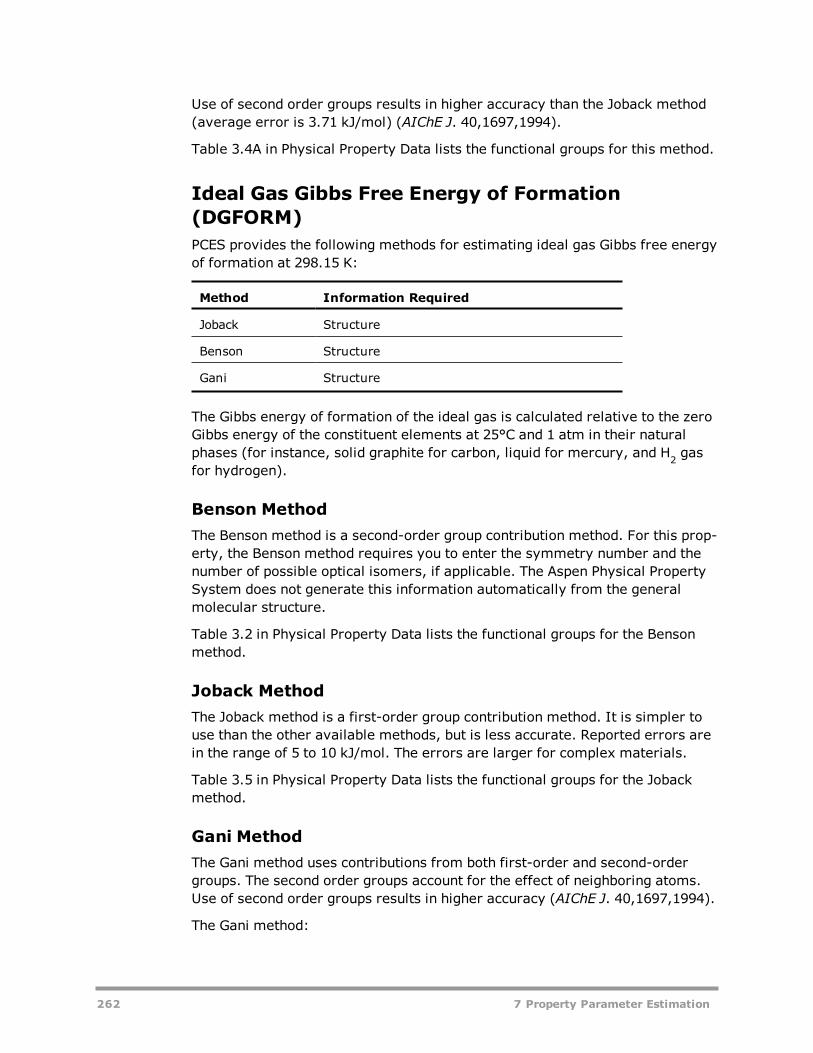
Use of second order groups results in higher accuracy than the Joback method(average error is 3.71 kJ/mol) (AIChE J. 40,1697,1994).
Table 3.4A in Physical Property Data lists the functional groups for this method.
Ideal Gas Gibbs Free Energy of Formation(DGFORM)PCES provides the following methods for estimating ideal gas Gibbs free energyof formation at 298.15 K:
Method Information Required
Joback Structure
Benson Structure
Gani Structure
The Gibbs energy of formation of the ideal gas is calculated relative to the zeroGibbs energy of the constituent elements at 25°C and 1 atm in their naturalphases (for instance, solid graphite for carbon, liquid for mercury, and H2 gasfor hydrogen).
Benson MethodThe Benson method is a second-order group contribution method. For this prop-erty, the Benson method requires you to enter the symmetry number and thenumber of possible optical isomers, if applicable. The Aspen Physical PropertySystem does not generate this information automatically from the generalmolecular structure.
Table 3.2 in Physical Property Data lists the functional groups for the Bensonmethod.
Joback MethodThe Joback method is a first-order group contribution method. It is simpler touse than the other available methods, but is less accurate. Reported errors arein the range of 5 to 10 kJ/mol. The errors are larger for complex materials.
Table 3.5 in Physical Property Data lists the functional groups for the Jobackmethod.
Gani MethodThe Gani method uses contributions from both first-order and second-ordergroups. The second order groups account for the effect of neighboring atoms.Use of second order groups results in higher accuracy (AIChE J. 40,1697,1994).
The Gani method:
262 7 Property Parameter Estimation

l Is more complex to use than the Joback methodl Reports more accurate results than Joback (average error is 3.24 kJ/-mol)
Table 3.4A in Physical Property Data lists the functional groups for this method
Heat of Vaporization at TB (DHVLB)PCES estimates heat of vaporization at the normal boiling point by applying theWatson equation (DHVLWT) from the General Pure Component Heat of Vapor-ization correlation at TB.
Liquid Molar Volume at TB (VB)PCES estimates liquid molar volume at the normal boiling point by applying theRackett equation (RKTZRA) from the General Pure Component Liquid MolarVolume model at TB.
Standard Liquid Volume (VLSTD)PCES estimates standard liquid volume by applying the Rackett equation(RKTZRA) from the General Pure Component Liquid Molar Volume correlation at60° F.
Radius of Gyration (RGYR)PCES estimates radius of gyration from parachor (PARC).
Solubility Parameter (DELTA)The solubility parameter is calculated from the definition.
UNIQUAC R and Q Parameters (GMUQR, GMUQQ)PCES provides the Bondi method for estimating the UNIQUAC R and Q para-meters. This method requires only molecular structure as input. Table 3.3 inPhysical Property Data in the help lists the functional groups.
Parachor (PARC)PCES provides one method for estimating Parachor. The Parachor method is agroup-contribution method. The functional groups for this method are listed inTable 3.10 in Physical Property Data.
Ideal Gas Heat Capacity (CPIG)PCES provides three methods for estimating ideal gas heat capacity:
7 Property Parameter Estimation 263

Method Information Required
Data Ideal gas heat capacity data
Benson Structure
Joback Structure
PCES uses the Aspen equation from the General Pure Component Ideal GasHeat Capacity model for this property. Both the Benson and Joback methodsare group-contribution methods that apply to a wide range of compounds.
Do not use the Benson or Joback methods outside the temperature range of 280to 1100 K. Errors are generally less than 1 to 2%.
Benson MethodBenson is the recommended method. It accounts for the effect of neighboringatoms. In comparison with the Joback method, Benson:
l Is more complex to usel Reports more accurate results (average error 1.1% for 27 diverse com-pounds)
Table 3.2 in Physical Property Data lists the functional groups for the Bensonmethod.
Joback MethodThe Joback method is a first-order group contribution method. It is simpler touse than the Benson method, but is less accurate. Reported average error is1.4% for 28 diverse components.
Table 3.5 in Physical Property Data lists the functional groups for the Jobackmethod.
Data MethodThe Data method determines parameters for the ideal gas heat capacity poly-nomial. Experimental ideal gas heat capacity data are fitted. You enter this dataon the Data | Pure Component form.
Vapor Pressure (PL)PCES provides the following methods for estimating vapor pressure:
Method Information Required
Data Vapor pressure data
Riedel TB, TC, PC, (vapor pressure data)
264 7 Property Parameter Estimation
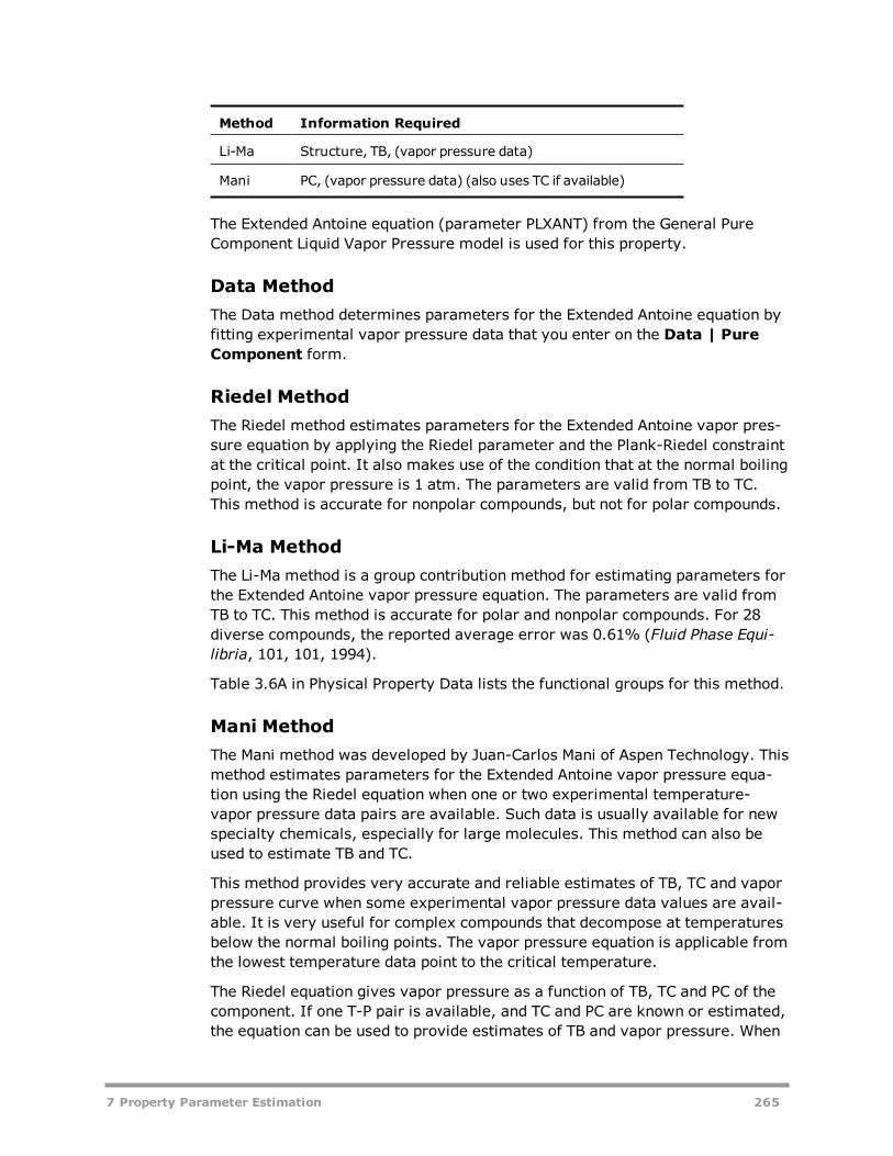
Method Information Required
Li-Ma Structure, TB, (vapor pressure data)
Mani PC, (vapor pressure data) (also uses TC if available)
The Extended Antoine equation (parameter PLXANT) from the General PureComponent Liquid Vapor Pressure model is used for this property.
Data MethodThe Data method determines parameters for the Extended Antoine equation byfitting experimental vapor pressure data that you enter on the Data | PureComponent form.
Riedel MethodThe Riedel method estimates parameters for the Extended Antoine vapor pres-sure equation by applying the Riedel parameter and the Plank-Riedel constraintat the critical point. It also makes use of the condition that at the normal boilingpoint, the vapor pressure is 1 atm. The parameters are valid from TB to TC.This method is accurate for nonpolar compounds, but not for polar compounds.
Li-Ma MethodThe Li-Ma method is a group contribution method for estimating parameters forthe Extended Antoine vapor pressure equation. The parameters are valid fromTB to TC. This method is accurate for polar and nonpolar compounds. For 28diverse compounds, the reported average error was 0.61% (Fluid Phase Equi-libria, 101, 101, 1994).
Table 3.6A in Physical Property Data lists the functional groups for this method.
Mani MethodThe Mani method was developed by Juan-Carlos Mani of Aspen Technology. Thismethod estimates parameters for the Extended Antoine vapor pressure equa-tion using the Riedel equation when one or two experimental temperature-vapor pressure data pairs are available. Such data is usually available for newspecialty chemicals, especially for large molecules. This method can also beused to estimate TB and TC.
This method provides very accurate and reliable estimates of TB, TC and vaporpressure curve when some experimental vapor pressure data values are avail-able. It is very useful for complex compounds that decompose at temperaturesbelow the normal boiling points. The vapor pressure equation is applicable fromthe lowest temperature data point to the critical temperature.
The Riedel equation gives vapor pressure as a function of TB, TC and PC of thecomponent. If one T-P pair is available, and TC and PC are known or estimated,the equation can be used to provide estimates of TB and vapor pressure. When
7 Property Parameter Estimation 265

two T-P pairs are available and PC is known or estimated, the equation canprovide estimates of TB, TC, and vapor pressure.
Heat of Vaporization (DHVL)PCES provides the following methods for estimating heat of vaporization:
Method Information Required
Data Heat of vaporization data
Definition TC, PC, PL, (Heat of vaporization data)
Vetere MW, TB, (Heat of vaporization data)
Gani Structure, (Heat of vaporization data)
Ducros Structure, (Heat of vaporization data)
Li-Ma Structure, TB, (Heat of vaporization data)
The Watson equation (parameter DHVLWT) from the General Pure ComponentHeat of Vaporization model is used for this property.
Data MethodThe Data method determines the Watson parameters by fitting experimentalheat of vaporization data that you enter on the Data | Pure Component form.
Definition MethodThe Definition method calculates heat of vaporization from the Clausius-Clapeyron equation. It requires vapor pressure, TC, and PC as input. The cal-culated heat of vaporization values are used to determine the parameters forthe Watson equation. When the Riedel method was used to estimate vapor pres-sure, reported average error for the heat of vaporization was 1.8% for 94 com-pounds.
Vetere MethodThe Vetere method estimates heat of vaporization at TB, then uses the Watsonequation to extrapolate heat of vaporization to TC. Reported average error is1.6%.
Gani MethodThe Gani method is a group contribution method for estimating heat of vapor-ization at 298K. It uses the Watson equation to extrapolate heat of vaporizationto TC. This method requires only molecular structure as input.
Table 3.4A in Physical Property Data lists the functional groups for this method.
266 7 Property Parameter Estimation

Ducros MethodThe Ducros method is a group contribution method for estimating heat of vapor-ization at 298K. It uses the Watson equation to extrapolate heat of vaporizationto TC (Thermochimica Acta, 36, 39, 1980; 44, 131, 1981; 54, 153, 1982; 75,329, 1984). This method:
l Uses more complex structure correctionl Can be applied to organo-metallic compounds
Table 3.3A in Physical Property Data lists the functional groups for this method.
Li-Ma MethodThe Li-Ma method is a group contribution method for estimating heat of vapor-ization at different temperatures. This method requires molecular structure andTB as input. Reported average error for 400 diverse compounds was 1.05%(Fluid Phase Equilibria, 1997).
Table 3.6A in Physical Property Data lists the functional groups for this method.
Liquid Molar Volume (VL)PCES provides three methods for estimating liquid molar volume:
Method Information Required
Data Liquidmolar volume data
Gunn-Yamada TC, PC.OMEGA
Le Bas Structure
The Rackett equation (parameter RKTZRA) from the General Pure ComponentLiquid Molar Volume model is used for this property.
Gunn-Yamada MethodThe Gunn-Yamada method estimates saturated liquid molar volume, when thereduced temperature is less than 0.99. The calculated values are used todetermine the Rackett parameter. This method:
l Applies to nonpolar and slightly polar compoundsl Is more accurate than the Le Bas method
Le Bas MethodThe Le Bas method estimates liquid molar volume at TB. The result is used todetermine the Rackett parameter. For 29 diverse compounds, an average errorof 3.9% is reported. This method requires only molecular structure as input.Table 3.6 in Physical Property Data lists the functional groups.
7 Property Parameter Estimation 267

Data MethodThe Data method determines the Rackett parameter by fitting the experimentalliquid molar volume data that you enter on the Data | Pure Component form.
Liquid Viscosity (MUL)PCES provides the following methods for estimating liquid viscosity:
Method Information Required
Data Liquid viscosity data
Orrick-Erbar Structure, MW, VL, ZC, TC, PC
Letsou-Stiel MW, TC, PC, OMEGA
The Andrade equation (parameter MULAND) from the General Pure ComponentLiquid Viscosity model is used for this property.
Orrick-Erbar MethodOrrick-Erbar is a group-contribution method that depends on liquid molarvolume. It is limited to low temperatures, ranging from above the freezingpoint to the reduced temperature of 0.75. This method:
l Is not reliable for highly branched structuresl Does not apply to inorganic liquids or sulfur compoundsl Reports an average error of 15% for 188 organic liquids
Table 3.9 in Physical Property Data lists the functional groups for this method.
Letsou-Stiel MethodThe Letsou-Stiel method is appropriate for high temperatures and for reducedtemperatures of 0.76 to 0.92. The average error is 3% for 14 liquids.
Data MethodThe Data method determines the Andrade parameters by fitting experimentalliquid viscosity data that you enter on the Data | Pure Component form.
Vapor Viscosity (MUV)PCES provides the following methods for estimating vapor viscosity:
Method Information Required
Data Vapor viscosity data
Reichenberg Structure, MW,TC, PC
268 7 Property Parameter Estimation

The DIPPR equation (parameter MUVDIP) from the General Pure ComponentVapor Viscosity correlation is used for this property.
Reichenberg MethodReichenberg is a group-contribution method. For nonpolar compounds, theexpected error is between 1 and 3%. For polar compounds, the errors arehigher, but usually less than 4%. Table 3.11 in Physical Property Data lists thefunctional groups for this method.
Data MethodThe Data method determines the General Pure Component Vapor Viscosity cor-relation parameters by fitting experimental vapor viscosity data you enter onthe Data | Pure Component form.
Liquid Thermal Conductivity (KL)PCES provides the following methods for estimating liquid thermal conductivity:
Method Information Required
Data Liquid thermal conductivity data
Sato-Riedel MW, TB, TC
The DIPPR equation (parameter KLDIP) from the General Pure ComponentLiquid Thermal Conductivity correlation is used for this property.
Sato-Riedel MethodWhen you use the Sato-Riedel method, accuracy varies widely from 1 to 20%for the compounds tested. The accuracy is poor for light and branched hydro-carbons.
Data MethodThe Data method determines the DIPPR liquid thermal conductivity correlationparameters. This method fits experimental liquid thermal conductivity data.Enter this data on the Data | Pure Component form.
Vapor Thermal Conductivity (KV)No estimation method is available for estimating vapor thermal conductivity.You can use the Data method to fit experimental data directly to the DIPPRvapor thermal conductivity correlation (parameter KVDIP). Use the Data |Pure Component form to enter experimental vapor thermal conductivity data.
7 Property Parameter Estimation 269

Surface Tension (SIGMA)PCES provides the following methods for estimating surface tension:
Method Information Required
Data Surface tension data
Brock-Bird TB, TC, PC
Macleod-Sugden TB, TC, PC, VL, PARC
Li-Ma Structure, TB
The DIPPR equation (parameter SIGDIP) from the General Pure ComponentLiquid Surface Tension correlation is used for this property.
Data MethodThe Data method determines the DIPPR surface tension correlation parametersby fitting experimental surface tension data. Enter this data on the Data |Pure Component form.
Brock-Bird MethodThe Brock-Bird method applies to non-hydrogen-bonded liquids. The expectederror is less than 5%.
Macleod-Sugden MethodThe Macleod-Sugden method applies to nonpolar, polar, and hydrogen-bondedliquids. For hydrogen-bonded liquids, errors are normally less than 5 to 10%.
Li-Ma MethodThe Li-Ma method is a group contribution method for estimating surface tensionat different temperature. This method requires only molecular structure and TBas input. Reported average error for 427 diverse compounds was 1.09% (FluidPhase Equilibria, 118, 13, 1996).
Table 3.6A in Physical Property Data lists the functional groups for this method.
Liquid Heat Capacity (CPL)PCES provides the following methods for estimating liquid heat capacity:
Method Information Required
Data Liquid heat capacity data
Ruzicka Structure
270 7 Property Parameter Estimation

The DIPPR equation (parameter CPLDIP) from the General Pure ComponentLiquid Heat Capacity correlation is used for this property.
Data MethodThe Data method determines the DIPPR liquid heat capacity correlation para-meters by fitting experimental liquid heat capacity data. Enter this data on theData | Pure Component form.
Ruzicka MethodThe Ruzicka method is a group contribution method for estimating parametersfor the DIPPR liquid heat capacity correlation. The parameters are valid fromthe melting point to the normal boiling point. This method requires only molecu-lar structure as input. For 9772 diverse compounds, reported average errorswere 1.9% and 2.9% for nonpolar and polar compounds, respectively (J. Phys.Chem. Ref. Data, 22, 597, 1993; 22, 619, 1993).
Table 3.11A in Physical Property Data lists the functional groups for thismethod.
Solid Heat Capacity (CPS)PCES provides the following methods for estimating solid heat capacity:
Method Information Required
Data Solid heat capacity data
Mostafa Structure
The Aspen equation (parameter CPSPO1) from the General Pure ComponentSolid Heat Capacity correlation is used for this property.
Data MethodThe Data method determines the solid heat capacity correlation parameters byfitting experimental liquid heat capacity data. You enter this data on the Data |Pure Component form.
Mostafa MethodThe Mostafa method is a group contribution method for estimating parametersfor the solid heat capacity correlation. This method is applied to solid inorganicsalts which are divided to cations, anions and ligands. Reported average errorsfor 664 diverse solid inorganic salts, was 3.18% (Ind. Eng. Chem. Res., 35,343, 1996).
Table 3.7A in Physical Property Data lists the functional groups for this method.
7 Property Parameter Estimation 271
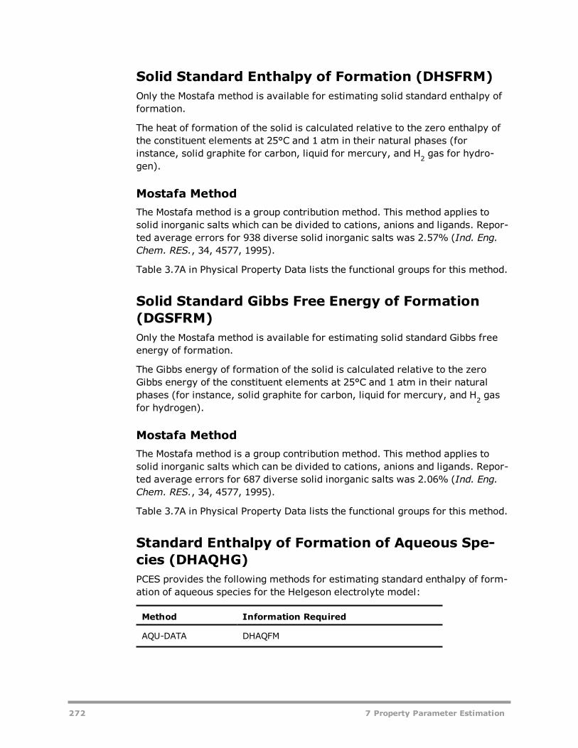
Solid Standard Enthalpy of Formation (DHSFRM)Only the Mostafa method is available for estimating solid standard enthalpy offormation.
The heat of formation of the solid is calculated relative to the zero enthalpy ofthe constituent elements at 25°C and 1 atm in their natural phases (forinstance, solid graphite for carbon, liquid for mercury, and H2 gas for hydro-gen).
Mostafa MethodThe Mostafa method is a group contribution method. This method applies tosolid inorganic salts which can be divided to cations, anions and ligands. Repor-ted average errors for 938 diverse solid inorganic salts was 2.57% (Ind. Eng.Chem. RES., 34, 4577, 1995).
Table 3.7A in Physical Property Data lists the functional groups for this method.
Solid Standard Gibbs Free Energy of Formation(DGSFRM)Only the Mostafa method is available for estimating solid standard Gibbs freeenergy of formation.
The Gibbs energy of formation of the solid is calculated relative to the zeroGibbs energy of the constituent elements at 25°C and 1 atm in their naturalphases (for instance, solid graphite for carbon, liquid for mercury, and H2 gasfor hydrogen).
Mostafa MethodThe Mostafa method is a group contribution method. This method applies tosolid inorganic salts which can be divided to cations, anions and ligands. Repor-ted average errors for 687 diverse solid inorganic salts was 2.06% (Ind. Eng.Chem. RES., 34, 4577, 1995).
Table 3.7A in Physical Property Data lists the functional groups for this method.
Standard Enthalpy of Formation of Aqueous Spe-cies (DHAQHG)PCES provides the following methods for estimating standard enthalpy of form-ation of aqueous species for the Helgeson electrolyte model:
Method Information Required
AQU-DATA DHAQFM
272 7 Property Parameter Estimation
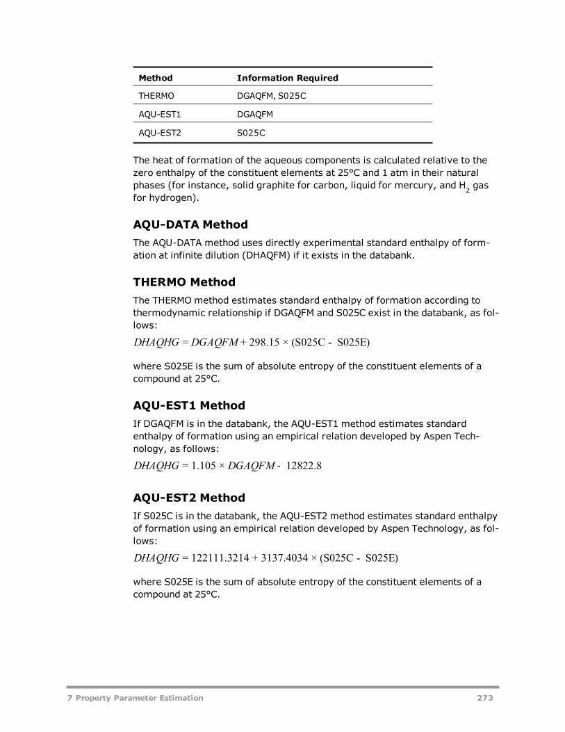
Method Information Required
THERMO DGAQFM, S025C
AQU-EST1 DGAQFM
AQU-EST2 S025C
The heat of formation of the aqueous components is calculated relative to thezero enthalpy of the constituent elements at 25°C and 1 atm in their naturalphases (for instance, solid graphite for carbon, liquid for mercury, and H2 gasfor hydrogen).
AQU-DATA MethodThe AQU-DATA method uses directly experimental standard enthalpy of form-ation at infinite dilution (DHAQFM) if it exists in the databank.
THERMO MethodThe THERMO method estimates standard enthalpy of formation according tothermodynamic relationship if DGAQFM and S025C exist in the databank, as fol-lows:
DHAQHG DGAQFM= + 298.15 × (S025C − S025E)
where S025E is the sum of absolute entropy of the constituent elements of acompound at 25°C.
AQU-EST1 MethodIf DGAQFM is in the databank, the AQU-EST1 method estimates standardenthalpy of formation using an empirical relation developed by Aspen Tech-nology, as follows:
DHAQHG DGAQFM= 1.105 × − 12822.8
AQU-EST2 MethodIf S025C is in the databank, the AQU-EST2 method estimates standard enthalpyof formation using an empirical relation developed by Aspen Technology, as fol-lows:
DHAQHG = 122111.3214 + 3137.4034 × (S025C − S025E)
where S025E is the sum of absolute entropy of the constituent elements of acompound at 25°C.
7 Property Parameter Estimation 273

Standard Gibbs Free Energy of Formation ofAqueous Species (DGAQHG)PCES provides the following methods for estimating standard Gibbs free energyof formation of aqueous species for the Helgeson electrolyte model:
Method Information Required
AQU-DATA DGAQFM
THERMO DHAQFM, S025C
AQU-EST1 DHAQFM
AQU-EST2 S025C
The Gibbs energy of formation of the aqueous components is calculated relativeto the zero Gibbs energy of the constituent elements at 25°C and 1 atm in theirnatural phases (for instance, solid graphite for carbon, liquid for mercury, andH2 gas for hydrogen).
AQU-DATA MethodThe AQU-DATA method uses directly experimental standard Gibbs free energyof formation at infinite dilution (DGAQFM) if it exists in the databank.
THERMO MethodIf DHAQFM and S025C are in the databank, the THERMO method estimatesstandard Gibbs free energy of formation according to thermodynamic rela-tionship, as follows:
DGAQHG DHAQFM= − 298.15 × (S025C − S025E)
where S025E is the sum of absolute entropy of the constituent elements of acompound at 25°C.
AQU-EST1 MethodIf DHAQFM is in the databank, the AQU-EST1 method estimates standard Gibbsfree energy of formation using an empirical relation developed by Aspen Tech-nology, as follows:
DGAQHGDHAQFM
=( + 12822.8)
1.105
AQU-EST2 MethodIf S025C is in the databank, the AQU-EST2 method estimates standard Gibbsfree energy of formation using an empirical relation developed by Aspen Tech-nology, as follows:
274 7 Property Parameter Estimation

DGAQHG S C S E= 122110.2752 + 2839.2534 × ( 025 − 025 )
where S025E is the sum of absolute entropy of the constituent elements of acompound at 25°C.
Absolute Entropy of Aqueous Species (S25HG)PCES provides the following methods for estimating absolute entropy ofaqueous species for the Helgeson electrolyte model:
Method Information Required
AQU-DATA S025C
THERMO DGAQFM, DHAQFM
AQU-EST1 DGAQFM
AQU-EST2 DHAQFM
AQU-DATA MethodThe AQU-DATA method uses directly the experimental absolute entropy(S025C) if it exists in the databank.
THERMO MethodIf DGAQFM and DHAQFM are in the databank, the THERMO method estimatesabsolute entropy according to thermodynamic relationship, as follows:
DHAQFM DGAQFMS25HG =
( − )
298.15+ S025E
where S025E is the sum of absolute entropy of the constituent elements of acompound at 25°C.
AQU-EST1 MethodIf DGAQFM is in the databank, the AQU-EST1 method estimates absoluteentropy using an empirical relation developed by Aspen Technology, as follows:
DGAQFMS25HG = 3.52205 × 10 × − 43.00788 + S025E− 4
where S025E is the sum of absolute entropy of the constituent elements of acompound at 25°C.
AQU-EST2 MethodIf DHAQFM is in the databank, the AQU-EST2 method estimates absoluteentropy using an empirical relation developed by Aspen Technology, as follows:
x DHAQFMS25HG = 3.187349 10 × − 38.9208 + S025E− 4
7 Property Parameter Estimation 275

Born Coefficient (OMEGHG)Only the Helgeson method is available for estimating the Born coefficient ofaqueous species for the Helgeson electrolyte model. This method requiresS25HG and CHARGE as input.
Helgeson Capacity Parameters (CHGPAR)PCES provides the following methods for estimating the Helgeson capacity para-meters of aqueous species for the Helgeson electrolyte model:
Method Information Required
HG-AUQ OMEGHG, CPAQ0
HG-CRIS OMEGHG, S25HG, CHARGE, IONTYP
HG-EST OMEGHG, S25HG
HG-AQU MethodThe HG-AQU method estimates the Helgeson capacity parameters from theinfinite dilution heat capacity CPAQ0.
HG-CRIS MethodThe HG-CRIS method estimates the Helgeson capacity parameters according tothe Criss-Cobble method.
HG-EST MethodThe HG-EST method estimates the Helgeson capacity parameters using anempirical relation developed by Aspen Technology.
Binary Parameters (WILSON, NRTL, UNIQ,SRKKIJ)PCES estimates binary parameters for the WILSON, NRTL, UNIQUAC, and SRKmodels, using infinite-dilution activity coefficients. Infinite-dilution activity coef-ficients can be supplied by:
l Laboratory data entered on the Data | Mixture form, with data type-e=GAMINF
l Estimation, using the UNIFAC, UNIF-LL, UNIF-DMD or UNIF-LBY method
SRKKIJ can also be estimated using the ASPEN method from critical volumewhen only light gases and hydrocarbons are present in the system.
For best results, use experimental infinite-dilution activity coefficient data. Ofthe four UNIFAC methods, the Dortmund method (UNIF-DMD) gives the mostaccurate estimate of infinite-dilution activity coefficients. This method is
276 7 Property Parameter Estimation
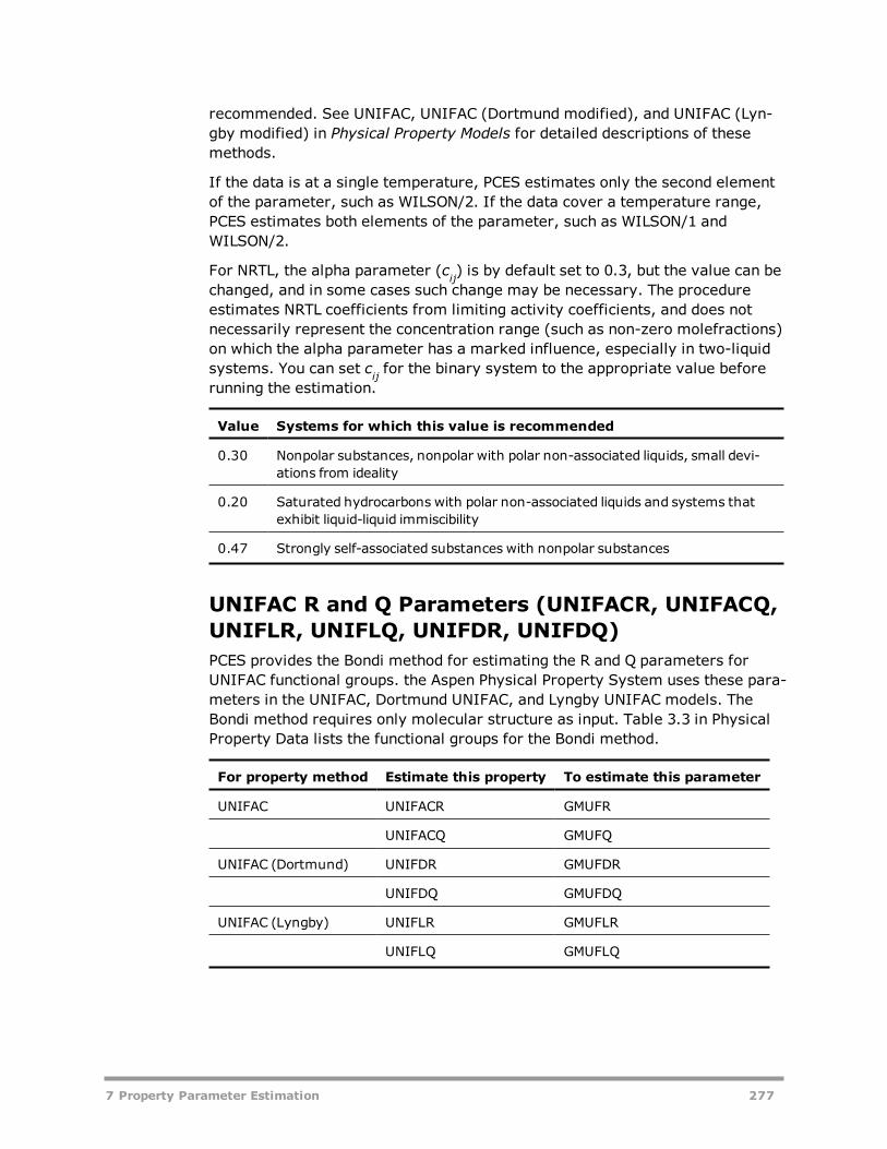
recommended. See UNIFAC, UNIFAC (Dortmund modified), and UNIFAC (Lyn-gby modified) in Physical Property Models for detailed descriptions of thesemethods.
If the data is at a single temperature, PCES estimates only the second elementof the parameter, such as WILSON/2. If the data cover a temperature range,PCES estimates both elements of the parameter, such as WILSON/1 andWILSON/2.
For NRTL, the alpha parameter (cij) is by default set to 0.3, but the value can bechanged, and in some cases such change may be necessary. The procedureestimates NRTL coefficients from limiting activity coefficients, and does notnecessarily represent the concentration range (such as non-zero molefractions)on which the alpha parameter has a marked influence, especially in two-liquidsystems. You can set cij for the binary system to the appropriate value beforerunning the estimation.
Value Systems for which this value is recommended
0.30 Nonpolar substances, nonpolar with polar non-associated liquids, small devi-ations from ideality
0.20 Saturated hydrocarbons with polar non-associated liquids and systems thatexhibit liquid-liquid immiscibility
0.47 Strongly self-associated substances with nonpolar substances
UNIFAC R and Q Parameters (UNIFACR, UNIFACQ,UNIFLR, UNIFLQ, UNIFDR, UNIFDQ)PCES provides the Bondi method for estimating the R and Q parameters forUNIFAC functional groups. the Aspen Physical Property System uses these para-meters in the UNIFAC, Dortmund UNIFAC, and Lyngby UNIFAC models. TheBondi method requires only molecular structure as input. Table 3.3 in PhysicalProperty Data lists the functional groups for the Bondi method.
For property method Estimate this property To estimate this parameter
UNIFAC UNIFACR GMUFR
UNIFACQ GMUFQ
UNIFAC (Dortmund) UNIFDR GMUFDR
UNIFDQ GMUFDQ
UNIFAC (Lyngby) UNIFLR GMUFLR
UNIFLQ GMUFLQ
7 Property Parameter Estimation 277

278 7 Property Parameter Estimation

Index 279
Index
A
absolute entropy 275aqueous species 275
acentric factor 260estimation 260
activity coefficient method 2, 10-11,16, 20-21
about 10advantages and disadvantages 21calculation of other properties 20for calculating phase equilibrium 2solids 16vapor-liquid equilibria 11
activity coefficient models 30-31,120, 130
characteristics of 30common models for 130electrolyte 31group contribution 31list of property methods 120molecular 30property models 30
AMINES property method 133API-METH property method 240-241API-TWU pseudocomponent property
method 240, 243APISOUR property method 136apparent component 211-212, 215approach 211-212mole fractions 215
Applications 16, 21liquid-liquid equilibrium 21petrochemical 17
Aspen OLI 149ASPEN pseudocomponent property
method 240-241
B
B-PITZER property method 146binary parameters 276estimation 276
BK10 property method 67-68Bondi method 277Born coefficient 276estimation 276
BWR-LS property method 83BWRS property method 85
C
calculations 160, 228, 247flash point 247properties 159three-phase 228
CHAO-SEA property method 67-68chemistry 209solution 209
classes of property methods 42COAL-LIQ property method 240, 242copolymer PC-SAFT EOS property
method 96critical compressibility factor 260estimation 260
critical pressure 257estimation 258
critical temperature 256estimation 257
critical volume 258estimation 259
D
data regression 221electrolytes 221
data sets 202, 205replacing models 202
Index

using in multiple propertymethods 205
diffusion coefficient propertymethods 193
dirty-water calculations 225-226, 228about 224organic phase properties 226phase properties 228specifying 225
E
ELECNRTL property method 137electrolyte calculation 209, 211, 216,
219, 221apparent component 211data regression 221equilibrium constants 216overview 209thermodynamic 219true component 211
electrolyte NRTL 220equation 220
electrolyte property methods 131,150
electrolytes calculation 209solution chemistry 209
ENRTL-HF property method 139ENRTL-HG property method 140ENRTL-RK property method 140ENRTL-SR property method 142enthalpy balances 34nonconventional components 34
enthalpy of formation estimationmethods 261, 271
ideal gas 261solid 271
equation-of-state method 2, 4-9, 22,82, 89
advantages and disadvantages 9calculation of properties 8common models for property meth-ods 89
critical solution temperature 7liquid-liquid equilibria 6method for phase equilibrium 3-4property methods for high-pressurehydrocarbon applications 82
property models 22
vapor-liquid equilibria 5equation-of-state models 22-23, 25about 22cubic equations of state 22vapor phase association 25virial equations of state 25
equations of state 113equilibrium constants 216molality versus mole fractionscale 216
EXT-API property method 244EXT-CAV property method 245EXT-TWU property method 244
F
flash point 247flexible and predictive property meth-
ods 90equation-of-state 90
FLPT-API method 247FLPT-PM method 247FLPT-TAG method 247free-water calculations 223, 225-226about 224organic phase properties 226phase properties 226specifying 225
G
Gibbs energy of formation estimationmethods 262, 272
aqueous species 272solid 272standard ideal gas 262
GRAYSON property method 67, 70GRAYSON2 property method 70group contribution activity coefficient
models 122UNIFAC 122
H
Hayden-O'Connell 118property methods 118
heat capacity 270liquid 270
280 Index
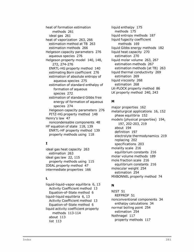
heat of formation estimationmethods 261
ideal gas 261heat of vaporization 263, 266estimation method at TB 263estimation methods 266
Helgeson capacity parameters 276aqueous species 276
Helgeson property model 140, 148,272, 274-276
ENRTL-HG property method 140estimating Born coefficient 276estimation of absolute entropy ofaqueous species 275
estimation of standard enthalpy offormation of aqueousspecies 272
estimation of standard Gibbs freeenergy of formation of aqueousspecies 274
Helgeson capacity parameters 276PITZ-HG property method 148
Henry's law 47noncondensable components 48
HF equation of state 118, 139ENRTL-HF property method 139property methods using 118
I
ideal gas heat capacity 263estimation 263
ideal gas law 22, 115property methods using 115
IDEAL property method 47intermediate properties 166
L
liquid-liquid-vapor equilibria 6, 13Activity Coefficient method 13Equation-of-State method 6
liquid-liquid equilibria 6, 13Activity Coefficient method 13Equation-of-State method 6
liquid activity coefficient propertymethods 113-114
about 113list 113
liquid enthalpy 175methods 175
liquid entropy methods 187liquid fugacity coefficient
methods 169liquid Gibbs energy methods 182liquid heat capacity 270estimation 270
liquid molar volume 263, 267estimation methods 267estimation methods (at TB) 263
liquid thermal conductivity 269estimation 269
liquid viscosity 268estimation 268
LK-PLOCK property method 86LK property method 240, 243
M
major properties 162metallurgical applications 16, 152phase equilibria 152
models (physical properties) 194,197, 202-203, 219
about 194definition 197electrolyte thermodynamics 219replacing 202specifications 203
molality scale 216equilibrium constants 216
molar volume methods 189mole fraction scale 216equilibrium constants 216
molecular weight 254estimation 254
MXBONNEL property method 74
N
NIST 51REFPROP 51
nonconventional components 34enthalpy calculations 34
normal boiling point 254estimation 254
Nothnagel 117property methods 117
Index 281

NRTL 120property methods 120
NRTL activity coefficient model 120
O
OLI property method 149
P
Parachor 263estimation 263
PC-SAFT property method 97, 99about 96option codes 99
PCES 251, 254, 256-258, 260-264,266-272, 274-276
estimating absolute entropy ofaqueous species 275
estimating acentric factor 260estimating binary parameters 276estimating critical pressure 257estimating critical temperature 256estimating critical volume 258estimating heat of vaporization 266estimating ideal gas Gibbs freeenergy of formation 262
estimating ideal gas heatcapacity 263
estimating ideal gas heat of form-ation 261
estimating liquid heat capacity 270estimating liquid molar volume 267estimating liquid thermal con-ductivity 269
estimating liquid viscosity 268estimating normal boiling point 254estimating solid heat capacity 271estimating standard enthalpy offormation of aqueousspecies 272
estimating standard Gibbs freeenergy of formation of aqueousspecies 274
estimating surface tension 270estimating vapor pressure 264estimating viscosity 268estimation methods 251
PENG-ROB property method 76
Peng-Robinson 76, 91equation-of-state 90property method 76
petroleum-tuned equation-of-stateproperty methods 75
petroleum fractions characterizationmethods 231, 234, 239-240
list of AspenTech extensions 234list of property methods 231property methods 240user models 239
petroleum mixtures 66, 81common models for 81property methods for 66, 81
petroleum property methods 240-245API-METH 241API-TWU 243ASPEN 241COAL-LIQ 242EXT-API 244EXT-TWU 244EXTCAV 245list 241LK 243
phase equilibrium calculation 3physical properties 161, 166, 195,
197calculation methods 166models 197properties 161routes 194
PITZ-HG property method 148Pitzer activity coefficient model 219Pitzer equation 219PITZER property method 144PR-BM property method 88predictive property methods 90, 111common models for 111equation-of-state 90
PRMHV2 property method 104property constant estimation
system 251estimation methods 251
property methods 1-2, 32-34, 41, 66-67, 75, 81-82, 89-90, 111, 113,130-131, 150, 152, 159, 200,204-205, 240
activity coefficient commonmodels 130
282 Index

classes of 42common models for equation-of-state 89
common models for petroleum mix-tures 81
creating 200, 204definition 41, 159descriptions 41diffusion coefficient 34equation-of-state 82flexible and predictive equation-of-state 90
flexible and predictive models 112for characterizing petroleum com-ponents 240
for electrolyte solutions 131, 150for K-value models 67for liquid fugacity 67for petroleum mixtures 66for solids 152liquid activity coefficient 113list 1modifications that can bemade 200
modifying 200petroleum-tuned equation-of-state 75
surface tension 34thermal conductivity 33thermodynamic 2transport 32using multiple data sets 205viscosity 33
property parameters 251, 254estimating 251-252estimation methods 254
PRWS property method 105pseudocomponents 231, 246-247ATOMNO and NOATOM 247NRTL and UNIQUAC binary para-meters 246
water solubility 246PSRK 106property method 106
R
radius of gyration 263estimation 263
Redlich-Kwong 91, 116equation-of-state 90, 116
REFPROP 51rigorous three-phase
calculations 223list of unit operation models 223
RK-ASPEN property method 107RK-SOAVE property method 77RKS-BM property method 88RKSMHV2 property method 108RKSWS property method 109routes 159, 194, 199-200, 203, 205about 194conflicting 203creating 205definition 159, 194modifying 205replacing 200tracing 199
S
solid enthalpy methods 180solid entropy methods 188solid fugacity coefficient
methods 173solid Gibbs energy methods 185solid heat capacity 271estimation 271
solid standard enthalpy offormation 272
estimation 272solid standard Gibbs free energy of
formation 272estimation 272
SOLIDS property method 152solubility parameter 263estimation 263
solution chemistry 209SR-POLAR property method 110SRK-KD property method 80SRK-ML property method 80SRK property method 78standard enthalpy of formation 261,
272aqueous species 272estimation methods 261
Index 283

standard Gibbs free energy of form-ation 262, 274
aqueous species 274estimation methods 262
standard heat of formation 261estimation methods 261
standard liquid volume 263estimation 263
STEAM-TA property method 156steam tables 155list 155property methods 155
STEAMNBS property method 156STMNBS2 property method 156subordinate properties 163surface tension 34, 270estimation 270property methods 34
surface tension methods 194
T
TC parameter 256estimation 257
thermal conductivity 33property method 33
thermal conductivity methods 192thermodynamic property 2methods 2
three-phase calculations 228rigorous calculations 228
transport property 32-34diffusion coefficient 34methods 32surface tension 34thermal conductivity 33viscosity 33
true component approach 211-212
U
UNIFAC 122, 277activity coefficient model 122R and Q parameters estimation 277
UNIFAC property methods 122UNIQUAC 124, 263activity coefficient model 124R and Q parameters estimationmethod 263
UNIQUAC property methods 125
unit operation models 223rigorous three-phasecalculations 223
V
Van Laar activity coefficientmodel 126
Van Laar property methods 127vapor-liquid equilibria 5, 11Activity Coefficient method 11Equation-of-State method 5
vapor enthalpy methods 174vapor entropy methods 186vapor fugacity coefficient
methods 169vapor Gibbs energy methods 181vapor phase association model 25vapor pressure 264estimation 264
vapor thermal conductivity 269estimation 269
vapor viscosity 268estimation 268
viscosity 33, 268estimation 268property method 33
viscosity methods 190VPA/IK-CAPE equation of state 119
W
water solubility in petroleumfractions 246
Wilson activity coefficient model 128Wilson property methods 128
Z
ZC 260Zemaitis equation 220
284 Index