bayesian decision theory - rochester institute of technology
TRANSCRIPT
Bayesian Decision Theory
Prof. Richard Zanibbi
Bayesian Decision Theory
The Basic Idea
To minimize errors, choose the least risky class, i.e. the class for which the expected loss is smallest
Assumptions
Problem posed in probabilistic terms, and all relevant probabilities are known
2
Probability Mass vs. Probability Density Functions
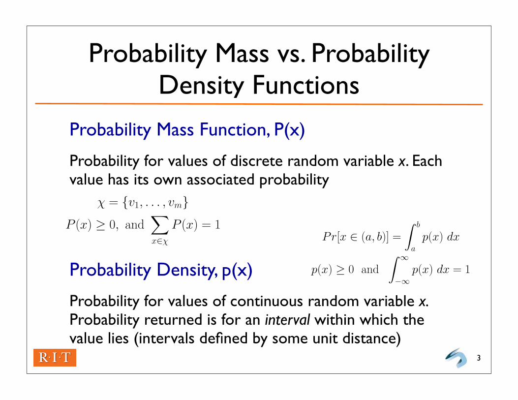
Probability Mass Function, P(x)
Probability for values of discrete random variable x. Each value has its own associated probability
Probability Density, p(x)
Probability for values of continuous random variable x. Probability returned is for an interval within which the value lies (intervals defined by some unit distance)
3
χ = {v1, . . . , vm}
P (x) ≥ 0, and∑
x∈χ
P (x) = 1
Pr[x ∈ (a, b)] =
∫ b
ap(x) dx
p(x) ≥ 0 and
∫ ∞
−∞p(x) dx = 1
1
χ = {v1, . . . , vm}
P (x) ≥ 0, and∑
x∈χ
P (x) = 1
Pr[x ∈ (a, b)] =
∫ b
ap(x) dx
p(x) ≥ 0 and
∫ ∞
−∞p(x) dx = 1
1

Prior ProbabilityDefinition ( P( w ) )
The likelihood of a value for a random variable representing the state of nature (true class for the current input), in the absence of other information
• Informally, “what percentage of the time state X occurs”
Example
The prior probability that an instance taken from two classes is provided as input, in the absence of any features (e.g. P(cat) = 0.3, P(dog) = 0.7)
4
Class-Conditional Probability Density Function (for Continuous Features)
Definition ( p( x | w ) )
The probability of a value for continuous random variable x, given a state of nature in w
• For each value of x, we have a different class-conditional pdf for each class in w (example next slide)
5
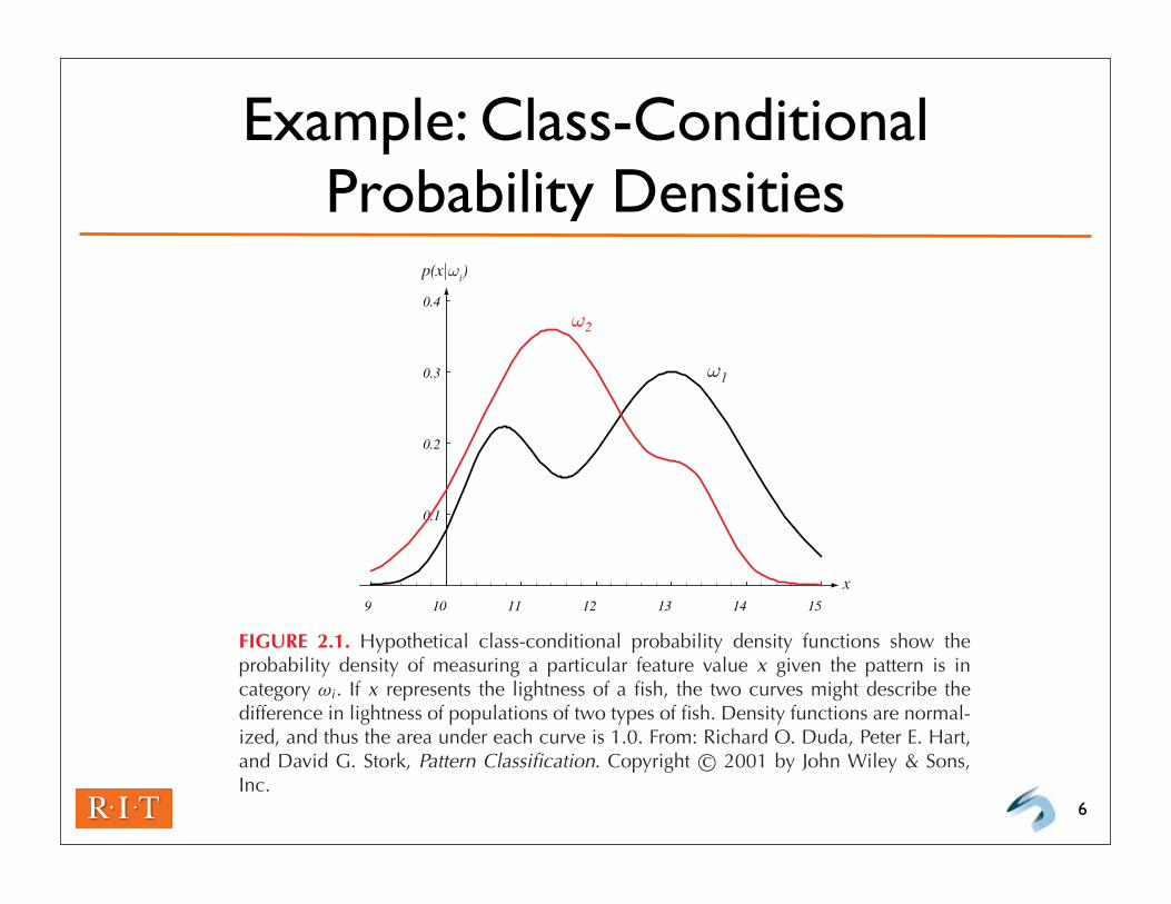
Example: Class-Conditional Probability Densities
6
9 10 11 12 13 14 15
0.1
0.2
0.3
0.4
p(x|ωi)
x
ω1
ω2
FIGURE 2.1. Hypothetical class-conditional probability density functions show theprobability density of measuring a particular feature value x given the pattern is incategory ωi . If x represents the lightness of a fish, the two curves might describe thedifference in lightness of populations of two types of fish. Density functions are normal-ized, and thus the area under each curve is 1.0. From: Richard O. Duda, Peter E. Hart,and David G. Stork, Pattern Classification. Copyright c© 2001 by John Wiley & Sons,Inc.

Bayes Formula
Purpose
Convert class prior and class-conditional densities to a posterior probability for a class: the probability of a class given the input features (‘post-observation’)
7
posterior = likelihood x prior evidence
P (ωj|x) =p(x|ωj)P (wj)
p(x)
where p(x) =c∑
j=1
p(x|ωj)P (ωj)
2
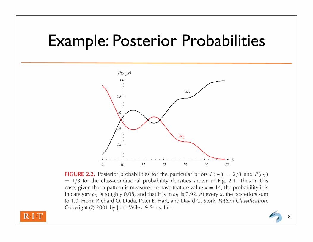
Example: Posterior Probabilities
8
0.2
0.4
0.6
0.8
1
P(ωi|x)
x
ω1
ω2
9 10 11 12 13 14 15
FIGURE 2.2. Posterior probabilities for the particular priors P(ω1) = 2/3 and P(ω2)
= 1/3 for the class-conditional probability densities shown in Fig. 2.1. Thus in thiscase, given that a pattern is measured to have feature value x = 14, the probability it isin category ω2 is roughly 0.08, and that it is in ω1 is 0.92. At every x, the posteriors sumto 1.0. From: Richard O. Duda, Peter E. Hart, and David G. Stork, Pattern Classification.Copyright c© 2001 by John Wiley & Sons, Inc.
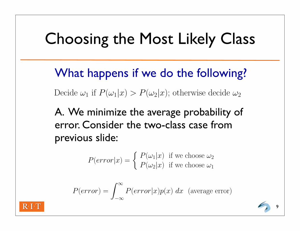
Choosing the Most Likely Class
What happens if we do the following?
A. We minimize the average probability of error. Consider the two-class case from previous slide:
9
P (ωj|x) =p(x|ωj)P (wj)
p(x)
where p(x) =c∑
j=1
p(x|ωj)P (ωj)
P (error|x) =
{P (ω1|x) if we choose ω2
P (ω2|x) if we choose ω1
P (error) =
∫ ∞
−∞P (error|x)p(x) dx (average error)
2
P (ωj|x) =p(x|ωj)P (wj)
p(x)
where p(x) =c∑
j=1
p(x|ωj)P (ωj)
P (error|x) =
{P (ω1|x) if we choose ω2
P (ω2|x) if we choose ω1
P (error) =
∫ ∞
−∞P (error|x)p(x) dx (average error)
Decide ω1 if P (ω1|x) > P (ω2|x); otherwise decide ω2
2
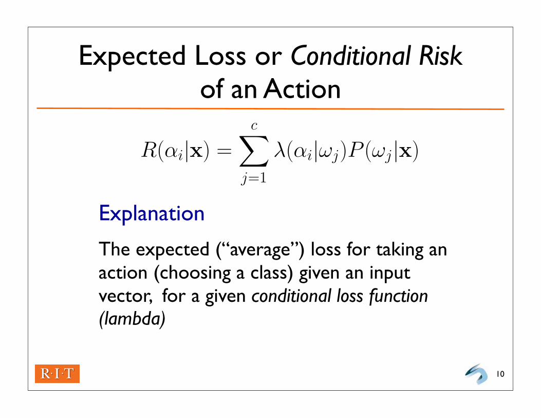
Expected Loss or Conditional Risk of an Action
Explanation
The expected (“average”) loss for taking an action (choosing a class) given an input vector, for a given conditional loss function (lambda)
10
R(αi|x) =c∑
j=1
λ(αi|ωj)P (ωj|x)
1
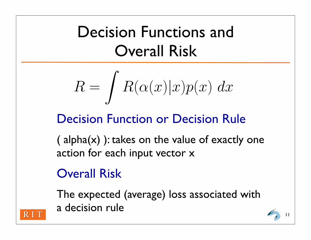
Decision Functions and Overall Risk
Decision Function or Decision Rule
( alpha(x) ): takes on the value of exactly one action for each input vector x
Overall Risk
The expected (average) loss associated with a decision rule
11
R(αi|x) =c∑
j=1
λ(αi|ωj)P (ωj|x)
R =
∫R(α(x)|x)p(x) dx
1

Bayes Decision Rule
Idea
Minimize the overall risk, by choosing the action with the least conditional risk for input vector x
Bayes Risk (R*)
The resulting overall risk produced using this procedure. This is the best performance that can be achieved given available information.
12
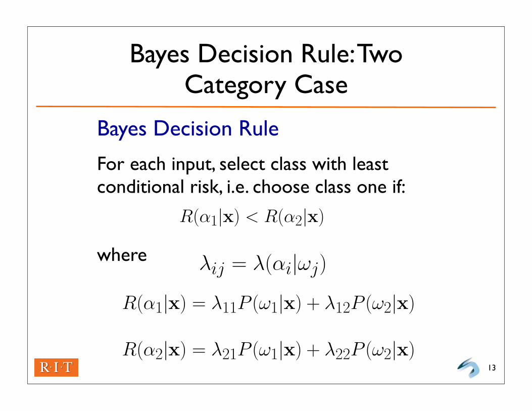
Bayes Decision Rule: Two Category Case
Bayes Decision Rule
For each input, select class with least conditional risk, i.e. choose class one if:
where
13
Bayesian Decision Rules
λij = λ(αi|ωj)
R(α1|x) < R(α2|x)
R(ω1|x) = λ11P (ω1|x) + λ12P (ω2|x)
R(ω2|x) = λ21P (ω1|x) + λ22P (ω2|x)
(λ21 − λ11)P (ω1|x) > (λ12 − λ22)P (ω2|x)
(λ21 − λ11)p(x|ω1)P (ω1) > (λ12 − λ22)p(x|ω2)P (ω2)
p(x|ω1)
p(x|ω2)>
λ12 − λ22
λ21 − λ11
P (ω2)
P (ω1)
1
Bayesian Decision Rules
λij = λ(αi|ωj)
R(α1|x) < R(α2|x)
R(α1|x) = λ11P (ω1|x) + λ12P (ω2|x)
R(α2|x) = λ21P (ω1|x) + λ22P (ω2|x)
(λ21 − λ11)P (ω1|x) > (λ12 − λ22)P (ω2|x)
(λ21 − λ11)p(x|ω1)P (ω1) > (λ12 − λ22)p(x|ω2)P (ω2)
p(x|ω1)
p(x|ω2)>
λ12 − λ22
λ21 − λ11
P (ω2)
P (ω1)
1
Bayesian Decision Rules
λij = λ(αi|ωj)
R(α1|x) < R(α2|x)
R(α1|x) = λ11P (ω1|x) + λ12P (ω2|x)
R(α2|x) = λ21P (ω1|x) + λ22P (ω2|x)
(λ21 − λ11)P (ω1|x) > (λ12 − λ22)P (ω2|x)
(λ21 − λ11)p(x|ω1)P (ω1) > (λ12 − λ22)p(x|ω2)P (ω2)
p(x|ω1)
p(x|ω2)>
λ12 − λ22
λ21 − λ11
P (ω2)
P (ω1)
1
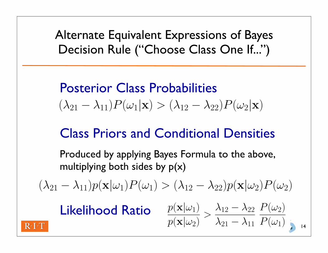
Alternate Equivalent Expressions of Bayes Decision Rule (“Choose Class One If...”)
Posterior Class Probabilities
Class Priors and Conditional DensitiesProduced by applying Bayes Formula to the above, multiplying both sides by p(x)
Likelihood Ratio14
Bayesian Decision Rules
λij = λ(αi|ωj)
R(α1|x) < R(α2|x)
R(α1|x) = λ11P (ω1|x) + λ12P (ω2|x)
R(α2|x) = λ21P (ω1|x) + λ22P (ω2|x)
(λ21 − λ11)P (ω1|x) > (λ12 − λ22)P (ω2|x)
(λ21 − λ11)p(x|ω1)P (ω1) > (λ12 − λ22)p(x|ω2)P (ω2)
p(x|ω1)
p(x|ω2)>
λ12 − λ22
λ21 − λ11
P (ω2)
P (ω1)
1
Bayesian Decision Rules
λij = λ(αi|ωj)
R(α1|x) < R(α2|x)
R(α1|x) = λ11P (ω1|x) + λ12P (ω2|x)
R(α2|x) = λ21P (ω1|x) + λ22P (ω2|x)
(λ21 − λ11)P (ω1|x) > (λ12 − λ22)P (ω2|x)
(λ21 − λ11)p(x|ω1)P (ω1) > (λ12 − λ22)p(x|ω2)P (ω2)
p(x|ω1)
p(x|ω2)>
λ12 − λ22
λ21 − λ11
P (ω2)
P (ω1)
1
Bayesian Decision Rules
λij = λ(αi|ωj)
R(α1|x) < R(α2|x)
R(α1|x) = λ11P (ω1|x) + λ12P (ω2|x)
R(α2|x) = λ21P (ω1|x) + λ22P (ω2|x)
(λ21 − λ11)P (ω1|x) > (λ12 − λ22)P (ω2|x)
(λ21 − λ11)p(x|ω1)P (ω1) > (λ12 − λ22)p(x|ω2)P (ω2)
p(x|ω1)
p(x|ω2)>
λ12 − λ22
λ21 − λ11
P (ω2)
P (ω1)
1
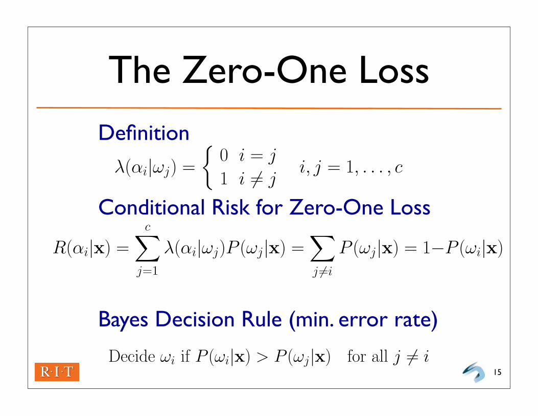
The Zero-One LossDefinition
Conditional Risk for Zero-One Loss
Bayes Decision Rule (min. error rate)
15
1 Minimum Error Rate Classification
λ(αi|ωj) =
{0 i = j1 i != j
i, j = 1, . . . , c
R(αi|x) =c∑
j=1
λ(αi|ωj)P (ωj|x) =∑
j !=i
P (ωj|x) = 1−P (ωi|x)
Decide ωi if P (ωi|x) > P (ωj|x) for all j != i
2 Multicategory case (revisited)
gi(x) > gj(x) for all j != i
gi(x) = −R(αi|x)gi(x) = P (ωi|x)
gi(x) = P (ωi|x) =p(x|ωi)P (ωi)∑c
j=1 p(x|ωj)P (ωj)gi(x) = p(x|ωi)P (ωi)gi(x) = ln p(x|ωi) + ln P (ωi)
2
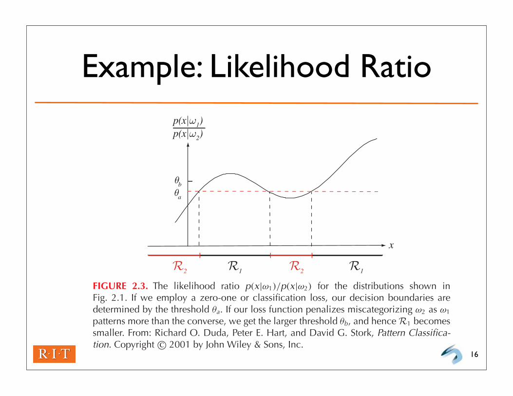
Example: Likelihood Ratio
16
x
θa
p(x|ω1)p(x|ω2)
θb
R1R2 R1R2
FIGURE 2.3. The likelihood ratio p(x|ω1)/p(x|ω2) for the distributions shown inFig. 2.1. If we employ a zero-one or classification loss, our decision boundaries aredetermined by the threshold θa. If our loss function penalizes miscategorizing ω2 as ω1
patterns more than the converse, we get the larger threshold θb, and hence R1 becomessmaller. From: Richard O. Duda, Peter E. Hart, and David G. Stork, Pattern Classifica-tion. Copyright c© 2001 by John Wiley & Sons, Inc.
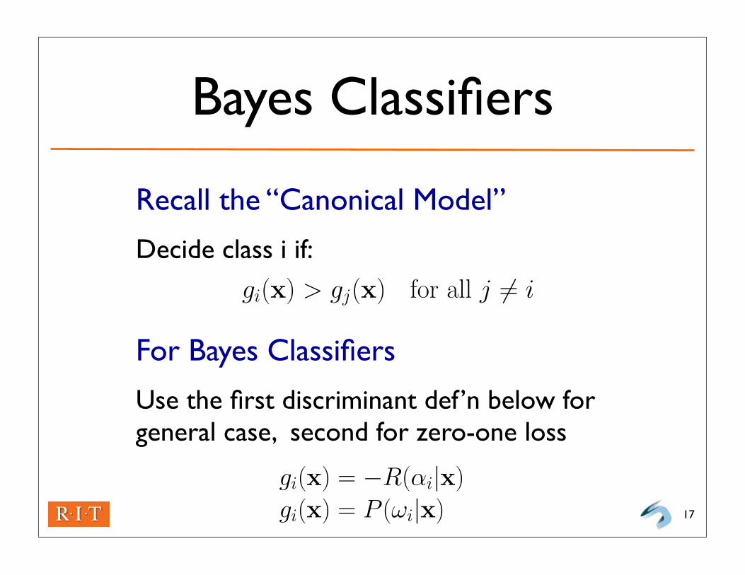
Bayes Classifiers
Recall the “Canonical Model”
Decide class i if:
For Bayes Classifiers
Use the first discriminant def’n below for general case, second for zero-one loss
17
1 Minimum Error Rate Classification
λ(αi|ωj) =
{0 i = j1 i != j
i, j = 1, . . . , c
R(αi|x) =c∑
j=1
λ(αi|ωj)P (ωj|x) =∑
j !=i
P (ωj|x) = 1−P (ωi|x)
Decide ωi if P (ωi|x) > P (ωj|x) for all j != i
2 Multicategory case (revisited)
gi(x) > gj(x) for all j != i
gi(x) = −R(αi|x)gi(x) = P (ωi|x)
gi(x) = P (ωi|x) =p(x|ωi)P (ωi)∑c
j=1 p(x|ωj)P (ωj)gi(x) = p(x|ωi)P (ωi)gi(x) = ln p(x|ωi) + ln P (ωi)
2

Equivalent Discriminants for Zero-One Loss (Minimum-Error-Rate)
Trade-off
Simplicity of understanding vs. computation
18
1 Minimum Error Rate Classification
λ(αi|ωj) =
{0 i = j1 i != j
i, j = 1, . . . , c
R(αi|x) =c∑
j=1
λ(αi|ωj)P (ωj|x) =∑
j !=i
P (ωj|x) = 1−P (ωi|x)
Decide ωi if P (ωi|x) > P (ωj|x) for all j != i
2 Multicategory case (revisited)
gi(x) > gj(x) for all j != i
gi(x) = −R(αi|x)gi(x) = P (ωi|x)
gi(x) = P (ωi|x) =p(x|ωi)P (ωi)∑c
j=1 p(x|ωj)P (ωj)gi(x) = p(x|ωi)P (ωi)gi(x) = ln p(x|ωi) + ln P (ωi)
2
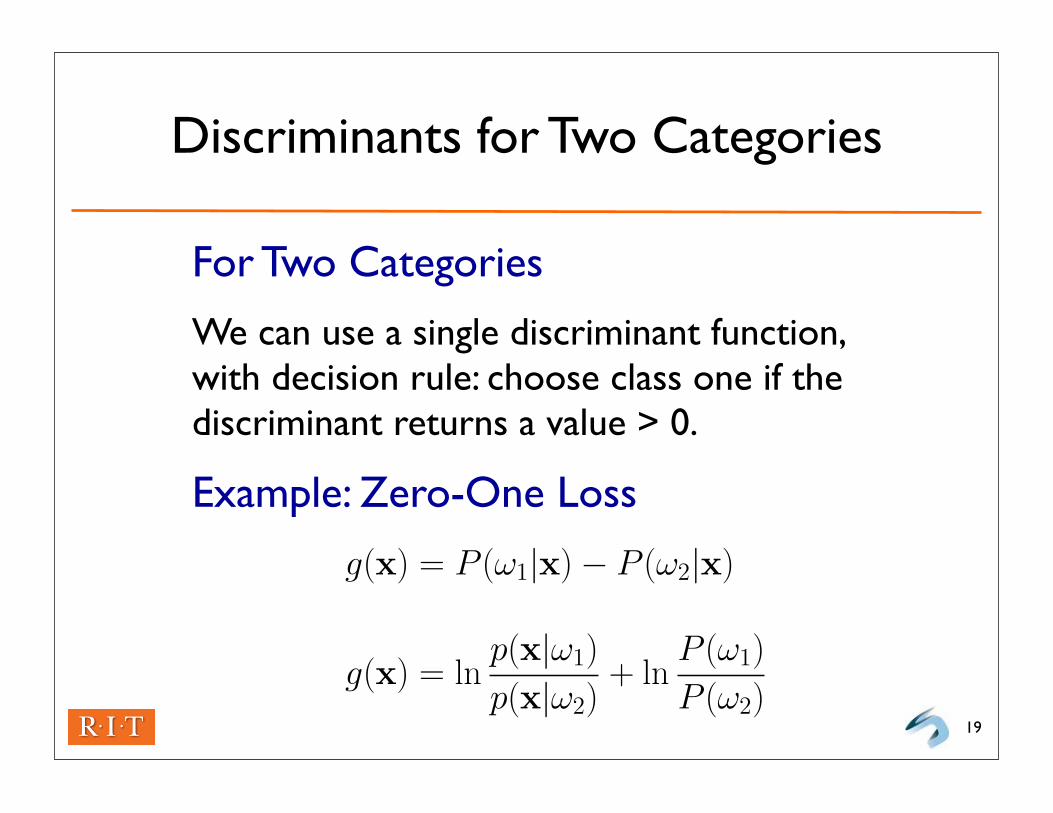
Discriminants for Two Categories
For Two Categories
We can use a single discriminant function, with decision rule: choose class one if the discriminant returns a value > 0.
Example: Zero-One Loss
19
3 two-category again
g(x) = P (ω1|x)− P (ω2|x)
g(x) = lnp(x|ω1)
p(x|ω2)+ ln
P (ω1)
P (ω2)
4 Gaussian (univariate normal)
P (x) =1√2πσ
exp
[−1
2
(x− µ
σ
)2]
µ =
∫ ∞
−∞x p(x) dx
σ2 =
∫ ∞
−∞(x− µ)2p(x) dx
5 Multivariate normal density
p(x) =1
(2π)d/2|Σ|1/2exp
[−1
2(x− µ)tΣ−1(x− µ)
]
µ =
∫ ∞
−∞x p(x) dx
Σ =
∫(x− µ)(x− µ)tp(x)dx
3
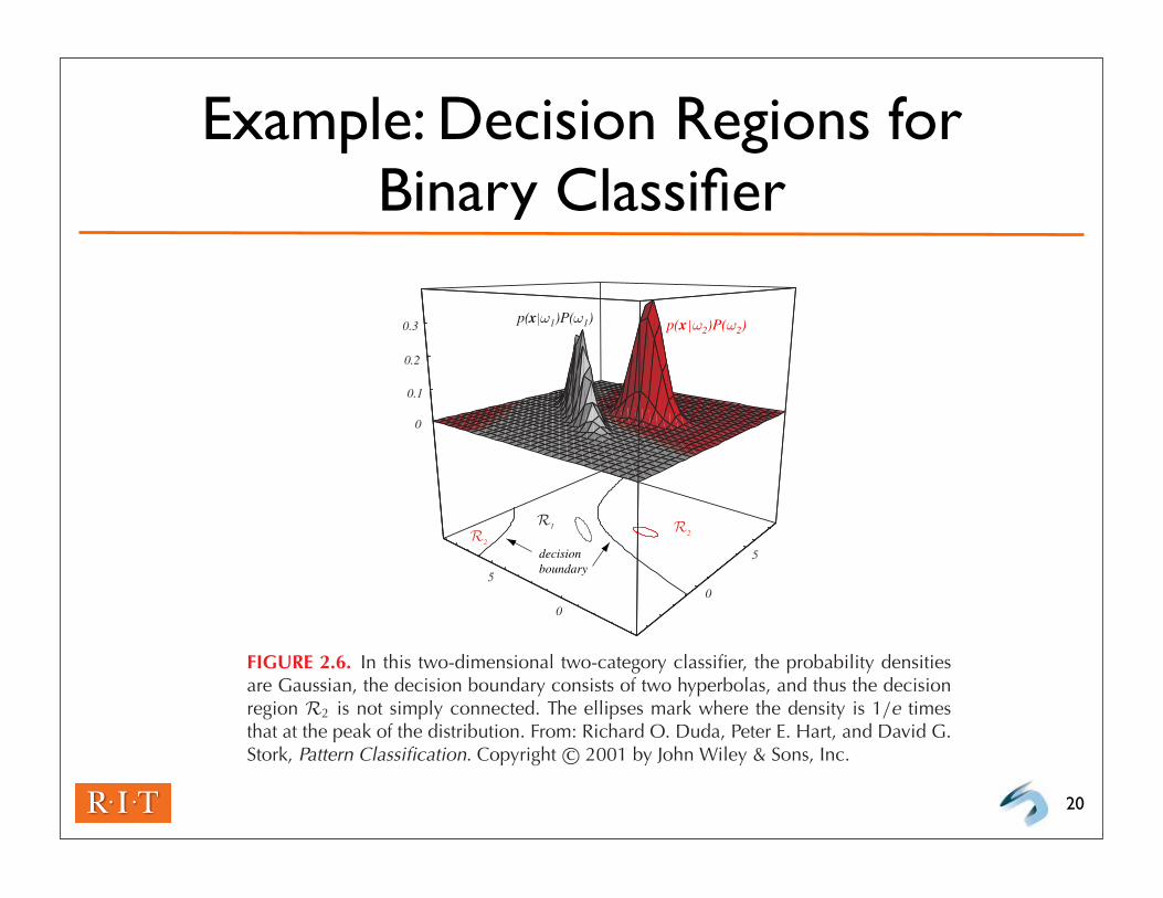
Example: Decision Regions for Binary Classifier
20
0
0.1
0.2
0.3
decisionboundary
p(x|ω2)P(ω2)
R1
R2
p(x|ω1)P(ω1)
R2
0
5
0
5
FIGURE 2.6. In this two-dimensional two-category classifier, the probability densitiesare Gaussian, the decision boundary consists of two hyperbolas, and thus the decisionregion R2 is not simply connected. The ellipses mark where the density is 1/e timesthat at the peak of the distribution. From: Richard O. Duda, Peter E. Hart, and David G.Stork, Pattern Classification. Copyright c© 2001 by John Wiley & Sons, Inc.
The (Univariate) Normal Distribution
21
Why are Gaussians so Useful?
They represent many probability distributions in nature quite accurately. In our case, when patterns can be represented as random variations of an ideal prototype (represented by the mean feature vector)
• Everyday examples: height, weight of a population
Univariate Normal Distribution
22
x
2.5% 2.5%
σ
p(x)
µ + σ µ + 2σµ - σµ - 2σ µ
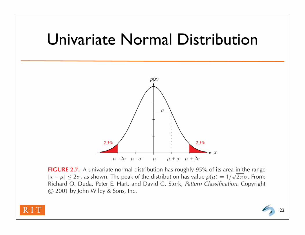
FIGURE 2.7. A univariate normal distribution has roughly 95% of its area in the range|x − µ| ≤ 2σ , as shown. The peak of the distribution has value p(µ) = 1/
√2πσ . From:
Richard O. Duda, Peter E. Hart, and David G. Stork, Pattern Classification. Copyrightc© 2001 by John Wiley & Sons, Inc.
Formal Definition
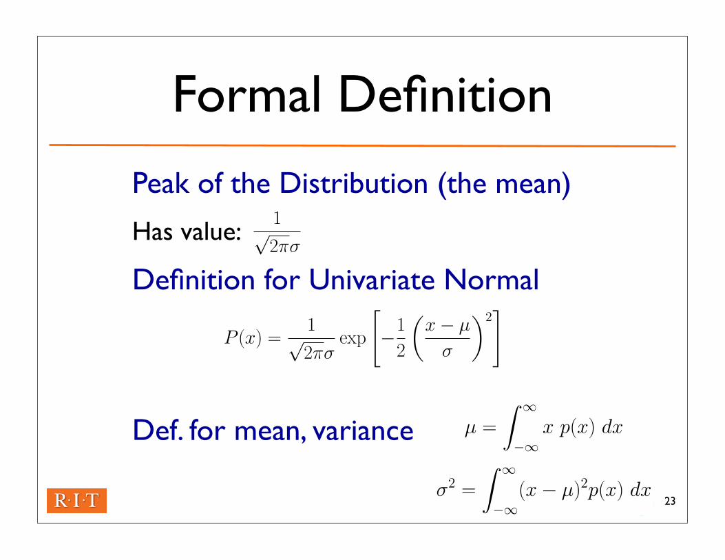
Peak of the Distribution (the mean)
Has value:
Definition for Univariate Normal
Def. for mean, variance
23
3 two-category again
g(x) = P (ω1|x)− P (ω2|x)
g(x) = lnp(x|ω1)
p(x|ω2)+ ln
P (ω1)
P (ω2)
4 Gaussian (univariate normal)
P (x) =1√2πσ
exp
[−1
2
(x− µ
σ
)2]
µ =
∫ ∞
−∞x p(x) dx
σ2 =
∫ ∞
−∞(x− µ)2p(x) dx
5 Multivariate normal density
p(x) =1
(2π)d/2|Σ|1/2exp
[−1
2(x− µ)tΣ−1(x− µ)
]
µ =
∫ ∞
−∞x p(x) dx
Σ =
∫(x− µ)(x− µ)tp(x)dx
3

Multivariate Normal Density
Informal Definition
A normal distribution over two or more variables (d variables/dimensions)
Formal Definition
24
3 two-category again
g(x) = P (ω1|x)− P (ω2|x)
g(x) = lnp(x|ω1)
p(x|ω2)+ ln
P (ω1)
P (ω2)
4 Gaussian (univariate normal)
P (x) =1√2πσ
exp
[−1
2
(x− µ
σ
)2]
µ =
∫ ∞
−∞x p(x) dx
σ2 =
∫ ∞
−∞(x− µ)2p(x) dx
5 Multivariate normal density
p(x) =1
(2π)d/2|Σ|1/2exp
[−1
2(x− µ)tΣ−1(x− µ)
]
µ =
∫ ∞
−∞x p(x) dx
Σ =
∫(x− µ)(x− µ)tp(x)dx
3

The Covariance Matrix ( )
For our purposes...
Assume matrix is positive definite, so the determinant of the matrix is always positive
Matrix Elements
• Main diagonal: variances for each individual variable
• Off-diagonal: covariances of each variable pairing i & j (note: values are repeated, as matrix is symmetric)
25
3 two-category again
g(x) = P (ω1|x)− P (ω2|x)
g(x) = lnp(x|ω1)
p(x|ω2)+ ln
P (ω1)
P (ω2)
4 Gaussian (univariate normal)
P (x) =1√2πσ
exp
[−1
2
(x− µ
σ
)2]
µ =
∫ ∞
−∞x p(x) dx
σ2 =
∫ ∞
−∞(x− µ)2p(x) dx
5 Multivariate normal density
p(x) =1
(2π)d/2|Σ|1/2exp
[−1
2(x− µ)tΣ−1(x− µ)
]
µ =
∫ ∞
−∞x p(x) dx
Σ =
∫(x− µ)(x− µ)tp(x)dx
3
Independence and Correlation
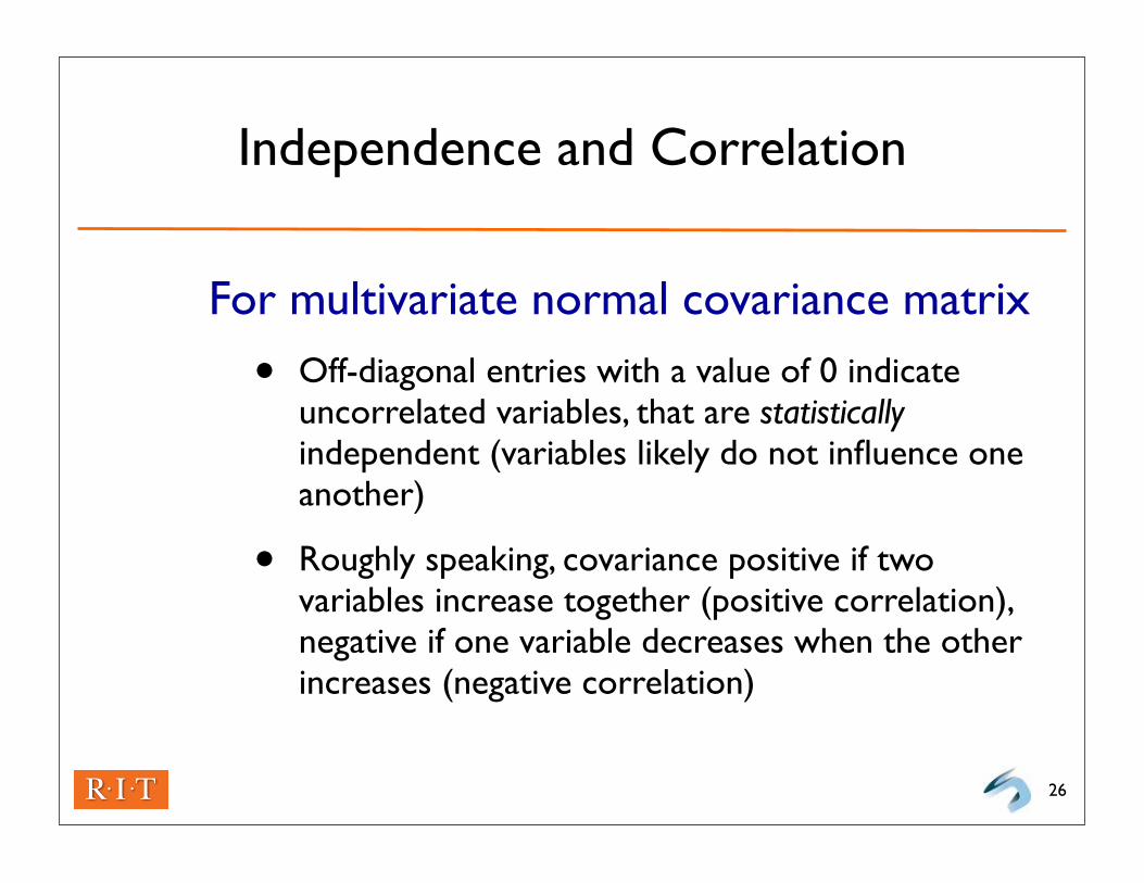
For multivariate normal covariance matrix
• Off-diagonal entries with a value of 0 indicate uncorrelated variables, that are statistically independent (variables likely do not influence one another)
• Roughly speaking, covariance positive if two variables increase together (positive correlation), negative if one variable decreases when the other increases (negative correlation)
26
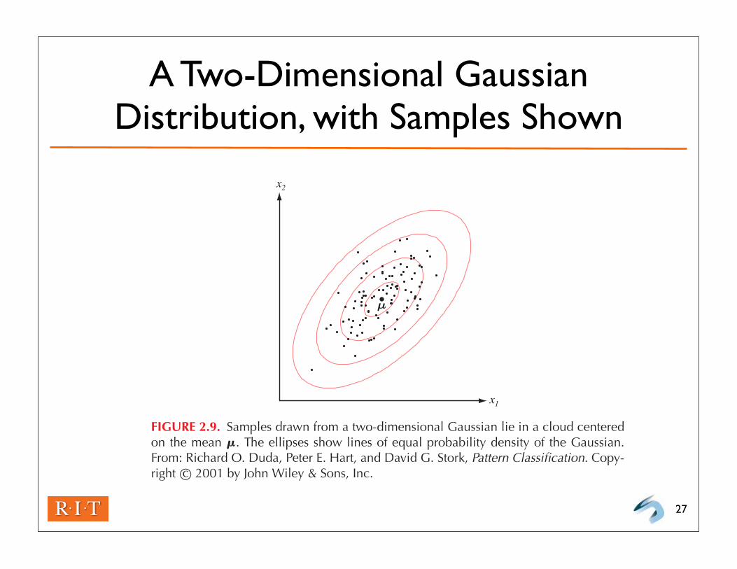
A Two-Dimensional Gaussian Distribution, with Samples Shown
27
x2
x1
µ
FIGURE 2.9. Samples drawn from a two-dimensional Gaussian lie in a cloud centeredon the mean !. The ellipses show lines of equal probability density of the Gaussian.From: Richard O. Duda, Peter E. Hart, and David G. Stork, Pattern Classification. Copy-right c© 2001 by John Wiley & Sons, Inc.
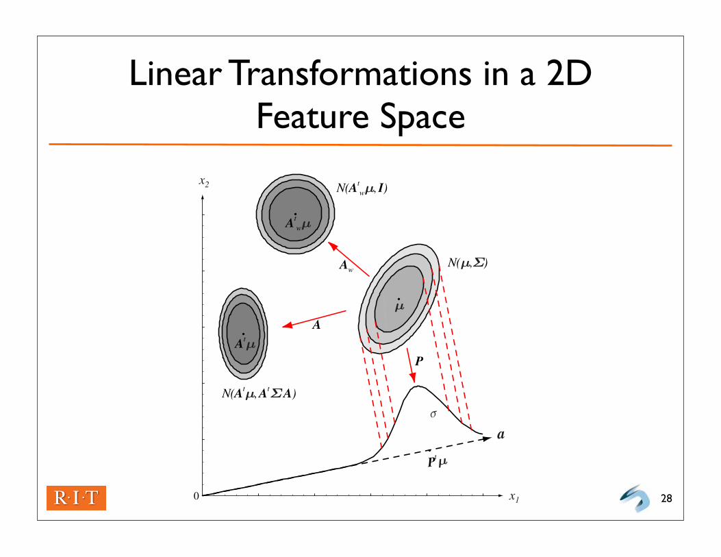
Linear Transformations in a 2D Feature Space
280
µ
Ptµ
Atµ
N(µ,Σ)
P
N(Atµ, AtΣ A)
A
a
N(Atwµ, I)
Aw
Atwµ
σ
x1
x2
FIGURE 2.8. The action of a linear transformation on the feature space will con-vert an arbitrary normal distribution into another normal distribution. One transforma-tion, A, takes the source distribution into distribution N(At!, At"A). Another lineartransformation—a projection P onto a line defined by vector a—leads to N(µ, σ 2) mea-sured along that line. While the transforms yield distributions in a different space, weshow them superimposed on the original x1x2-space. A whitening transform, Aw, leadsto a circularly symmetric Gaussian, here shown displaced. From: Richard O. Duda, Pe-ter E. Hart, and David G. Stork, Pattern Classification. Copyright c© 2001 by John Wiley& Sons, Inc.
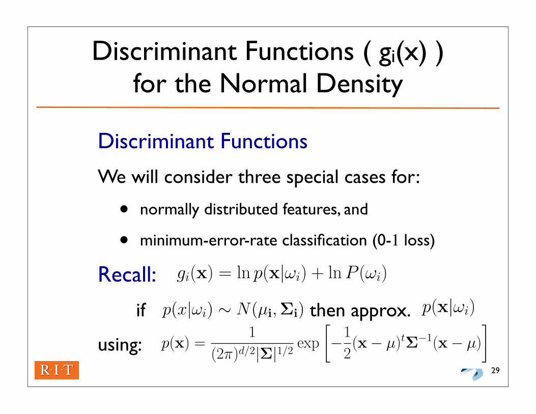
Discriminant Functions ( gi(x) ) for the Normal Density
29
Discriminant Functions
We will consider three special cases for:
• normally distributed features, and
• minimum-error-rate classification (0-1 loss)
Recall:
if then approx.
using:
1 Minimum Error Rate Classification
λ(αi|ωj) =
{0 i = j1 i != j
i, j = 1, . . . , c
R(αi|x) =c∑
j=1
λ(αi|ωj)P (ωj|x) =∑
j !=i
P (ωj|x) = 1−P (ωi|x)
Decide ωi if P (ωi|x) > P (ωj|x) for all j != i
2 Multicategory case (revisited)
gi(x) > gj(x) for all j != i
gi(x) = −R(αi|x)gi(x) = P (ωi|x)
gi(x) = P (ωi|x) =p(x|ωi)P (ωi)∑c
j=1 p(x|ωj)P (ωj)gi(x) = p(x|ωi)P (ωi)gi(x) = ln p(x|ωi) + ln P (ωi)
2
3 two-category again
g(x) = P (ω1|x)− P (ω2|x)
g(x) = lnp(x|ω1)
p(x|ω2)+ ln
P (ω1)
P (ω2)
4 Gaussian (univariate normal)
P (x) =1√2πσ
exp
[−1
2
(x− µ
σ
)2]
µ =
∫ ∞
−∞x p(x) dx
σ2 =
∫ ∞
−∞(x− µ)2p(x) dx
5 Multivariate normal density
p(x) =1
(2π)d/2|Σ|1/2exp
[−1
2(x− µ)tΣ−1(x− µ)
]
µ =
∫ ∞
−∞x p(x) dx
Σ =
∫(x− µ)(x− µ)tp(x)dx
3
1 Bayes Dec. Rules: Case I
p(x|ωi) ∼ N(µi,Σi)
gi(x) = −1
2(x− µi)
tΣi−1(x− µi)−
d
2ln 2π− 1
2ln |Σi| + ln P (ωi)
Σi = σ2I
|Σi| = σ2d,Σ−1i = (1/σ2)I
gi(x) = −(x− µi)t(x− µi)
2σ2 + ln P (ωi)
gi(x) = − 1
2σ2 [xtx− 2µt
ix + µitµi] + ln P (ωi)
gi(x) =1
σ2µitx− 1
2σ2µtiµi + ln P (ωi)
gi(x) = wtix + ωi0
gi(x) = gj(x)
wt(x− x0) = 0
(µi−µj)t(x−
(1
2(µi + µj)−
σ2
(µi − µj)t(µi − µj)ln
P (ωi)
P (ωj)(µi − µj)
))
1
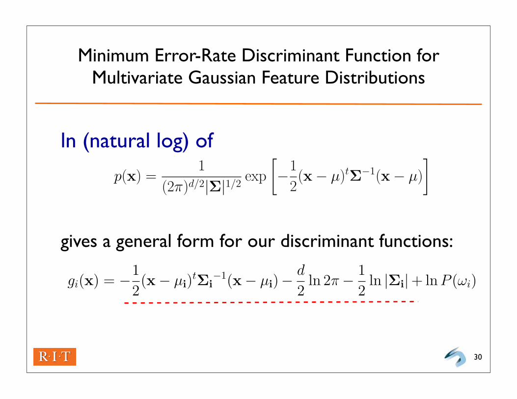
Minimum Error-Rate Discriminant Function for Multivariate Gaussian Feature Distributions
ln (natural log) of
gives a general form for our discriminant functions:
30
3 two-category again
g(x) = P (ω1|x)− P (ω2|x)
g(x) = lnp(x|ω1)
p(x|ω2)+ ln
P (ω1)
P (ω2)
4 Gaussian (univariate normal)
P (x) =1√2πσ
exp
[−1
2
(x− µ
σ
)2]
µ =
∫ ∞
−∞x p(x) dx
σ2 =
∫ ∞
−∞(x− µ)2p(x) dx
5 Multivariate normal density
p(x) =1
(2π)d/2|Σ|1/2exp
[−1
2(x− µ)tΣ−1(x− µ)
]
µ =
∫ ∞
−∞x p(x) dx
Σ =
∫(x− µ)(x− µ)tp(x)dx
3
1 Bayes Dec. Rules: Case I
p(x|ωi) ∼ N(ωi,Σi)
gi(x) = −1
2(x− µi)
tΣi−1(x− µi)−
d
2ln 2π− 1
2ln |Σi| + ln P (ωi)
2 Case II
3 Case III
1
Special Cases for Binary Classification
Purpose
Overview of commonly assumed cases for feature likelihood densities,
• Goal: eliminate common additive constants in discriminant functions. These do not affect the classification decision (i.e. define gi(x) providing “just the differences”)
• Also, look at resulting decision surfaces ( defined by gi(x) = gj(x) )
Three Special Cases
1. Statistically independent features, identically distributed Gaussians for each class
2. Identical covariances for each class
3. Arbitrary covariances31
1 Minimum Error Rate Classification
λ(αi|ωj) =
{0 i = j1 i != j
i, j = 1, . . . , c
R(αi|x) =c∑
j=1
λ(αi|ωj)P (ωj|x) =∑
j !=i
P (ωj|x) = 1−P (ωi|x)
Decide ωi if P (ωi|x) > P (ωj|x) for all j != i
2 Multicategory case (revisited)
gi(x) > gj(x) for all j != i
gi(x) = −R(αi|x)gi(x) = P (ωi|x)
gi(x) = P (ωi|x) =p(x|ωi)P (ωi)∑c
j=1 p(x|ωj)P (ωj)gi(x) = p(x|ωi)P (ωi)gi(x) = ln p(x|ωi) + ln P (ωi)
2
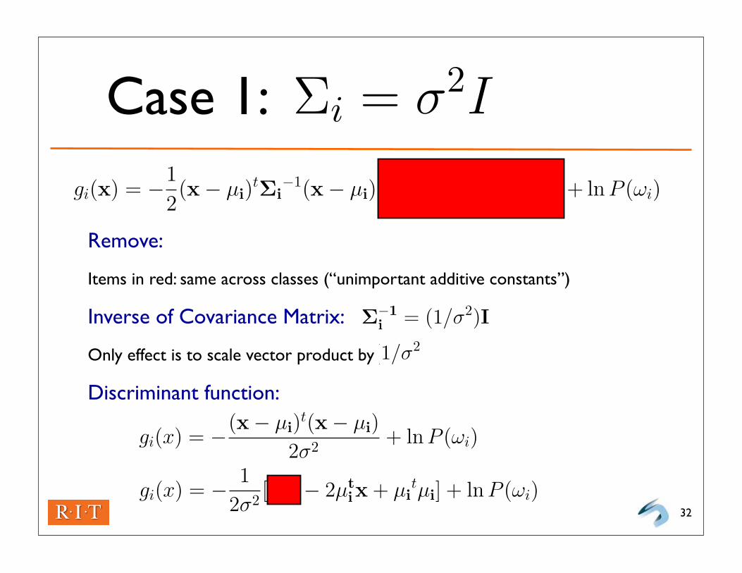
Case 1:
32
Remove:
Items in red: same across classes (“unimportant additive constants”)
Inverse of Covariance Matrix:
Only effect is to scale vector product by
Discriminant function:
1 Bayes Dec. Rules: Case I
p(x|ωi) ∼ N(ωi,Σi)
gi(x) = −1
2(x− µi)
tΣi−1(x− µi)−
d
2ln 2π− 1
2ln |Σi| + ln P (ωi)
Σi = σ2I
Σi = Σ
Σi = (arbitrary gaussian)
2 Case II
3 Case III
1
1 Bayes Dec. Rules: Case I
p(x|ωi) ∼ N(ωi,Σi)
gi(x) = −1
2(x− µi)
tΣi−1(x− µi)−
d
2ln 2π− 1
2ln |Σi| + ln P (ωi)
2 Case II
3 Case III
1
1 Bayes Dec. Rules: Case I
p(x|ωi) ∼ N(ωi,Σi)
gi(x) = −1
2(x− µi)
tΣi−1(x− µi)−
d
2ln 2π− 1
2ln |Σi| + ln P (ωi)
Σi = σ2I
|Σi| = σ2d,Σ−1i = (1/σ2)I
2 Case II
Σi = Σ
3 Case III
Σi = (arbitrary gaussian)
1
1 Bayes Dec. Rules: Case I
p(x|ωi) ∼ N(ωi,Σi)
gi(x) = −1
2(x− µi)
tΣi−1(x− µi)−
d
2ln 2π− 1
2ln |Σi| + ln P (ωi)
Σi = σ2I
|Σi| = σ2d,Σ−1i = (1/σ2)I
gi(x) = −(x− µi)t(x− µi)
2σ2 + ln P (ωi)
2 Case II
Σi = Σ
3 Case III
Σi = (arbitrary gaussian)
1
1 Bayes Dec. Rules: Case I
p(x|ωi) ∼ N(ωi,Σi)
gi(x) = −1
2(x− µi)
tΣi−1(x− µi)−
d
2ln 2π− 1
2ln |Σi| + ln P (ωi)
Σi = σ2I
|Σi| = σ2d,Σ−1i = (1/σ2)I
2 Case II
Σi = Σ
3 Case III
Σi = (arbitrary gaussian)
1
1 Bayes Dec. Rules: Case I
p(x|ωi) ∼ N(ωi,Σi)
gi(x) = −1
2(x− µi)
tΣi−1(x− µi)−
d
2ln 2π− 1
2ln |Σi| + ln P (ωi)
Σi = σ2I
|Σi| = σ2d,Σ−1i = (1/σ2)I
gi(x) = −(x− µi)t(x− µi)
2σ2 + ln P (ωi)
gi(x) = − 1
2σ2 [xtx− 2µt
ix + µitµi] + ln P (ωi)
2 Case II
Σi = Σ
3 Case III
Σi = (arbitrary gaussian)
1
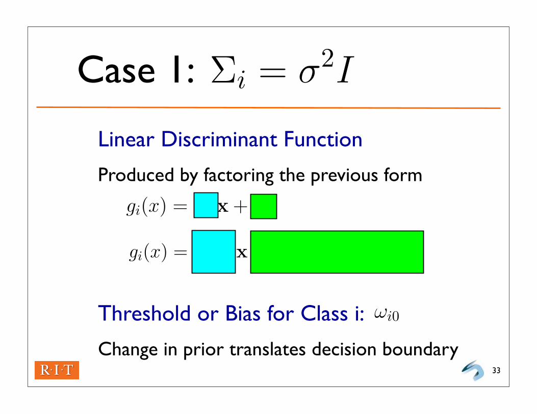
Case 1:
Linear Discriminant Function
Produced by factoring the previous form
Threshold or Bias for Class i:
Change in prior translates decision boundary33
1 Bayes Dec. Rules: Case I
p(x|ωi) ∼ N(ωi,Σi)
gi(x) = −1
2(x− µi)
tΣi−1(x− µi)−
d
2ln 2π− 1
2ln |Σi| + ln P (ωi)
Σi = σ2I
Σi = Σ
Σi = (arbitrary gaussian)
2 Case II
3 Case III
1
1 Bayes Dec. Rules: Case I
p(x|ωi) ∼ N(ωi,Σi)
gi(x) = −1
2(x− µi)
tΣi−1(x− µi)−
d
2ln 2π− 1
2ln |Σi| + ln P (ωi)
Σi = σ2I
|Σi| = σ2d,Σ−1i = (1/σ2)I
gi(x) = −(x− µi)t(x− µi)
2σ2 + ln P (ωi)
gi(x) = − 1
2σ2 [xtx− 2µt
ix + µitµi] + ln P (ωi)
gi(x) =1
σ2µix−1
2σ2µtiµi + ln P (ωi)
gi(x) = wtix + ωi0
1
1 Bayes Dec. Rules: Case I
p(x|ωi) ∼ N(ωi,Σi)
gi(x) = −1
2(x− µi)
tΣi−1(x− µi)−
d
2ln 2π− 1
2ln |Σi| + ln P (ωi)
Σi = σ2I
|Σi| = σ2d,Σ−1i = (1/σ2)I
gi(x) = −(x− µi)t(x− µi)
2σ2 + ln P (ωi)
gi(x) = − 1
2σ2 [xtx− 2µt
ix + µitµi] + ln P (ωi)
gi(x) =1
σ2µitx− 1
2σ2µtiµi + ln P (ωi)
gi(x) = wtix + ωi0
1
1 Bayes Dec. Rules: Case I
p(x|ωi) ∼ N(ωi,Σi)
gi(x) = −1
2(x− µi)
tΣi−1(x− µi)−
d
2ln 2π− 1
2ln |Σi| + ln P (ωi)
Σi = σ2I
|Σi| = σ2d,Σ−1i = (1/σ2)I
gi(x) = −(x− µi)t(x− µi)
2σ2 + ln P (ωi)
gi(x) = − 1
2σ2 [xtx− 2µt
ix + µitµi] + ln P (ωi)
gi(x) =1
σ2µitx− 1
2σ2µtiµi + ln P (ωi)
gi(x) = wtix + ωi0
1

Case 1:
Decision Boundary:
Notes
• Decision boundary goes through x0 along line between means, orthogonal to this line
• If priors equal, x0 between means (minimum distance classifier), otherwise x0 shifted
• If variance small relative to distance between means, priors have limited effect on boundary location 34
1 Bayes Dec. Rules: Case I
p(x|ωi) ∼ N(ωi,Σi)
gi(x) = −1
2(x− µi)
tΣi−1(x− µi)−
d
2ln 2π− 1
2ln |Σi| + ln P (ωi)
Σi = σ2I
Σi = Σ
Σi = (arbitrary gaussian)
2 Case II
3 Case III
1
1 Bayes Dec. Rules: Case I
p(x|ωi) ∼ N(ωi,Σi)
gi(x) = −1
2(x− µi)
tΣi−1(x− µi)−
d
2ln 2π− 1
2ln |Σi| + ln P (ωi)
Σi = σ2I
|Σi| = σ2d,Σ−1i = (1/σ2)I
gi(x) = −(x− µi)t(x− µi)
2σ2 + ln P (ωi)
gi(x) = − 1
2σ2 [xtx− 2µt
ix + µitµi] + ln P (ωi)
gi(x) =1
σ2µitx− 1
2σ2µtiµi + ln P (ωi)
gi(x) = wtix + ωi0
gi(x) = gj(x)
wt(x− x0) = 0
(µi−µj)t(x−
(1
2(µi + µj)−
σ2
(µi − µj)t(µi − µj)ln
P (ωi)
P (ωj)(µi − µj)
))
1
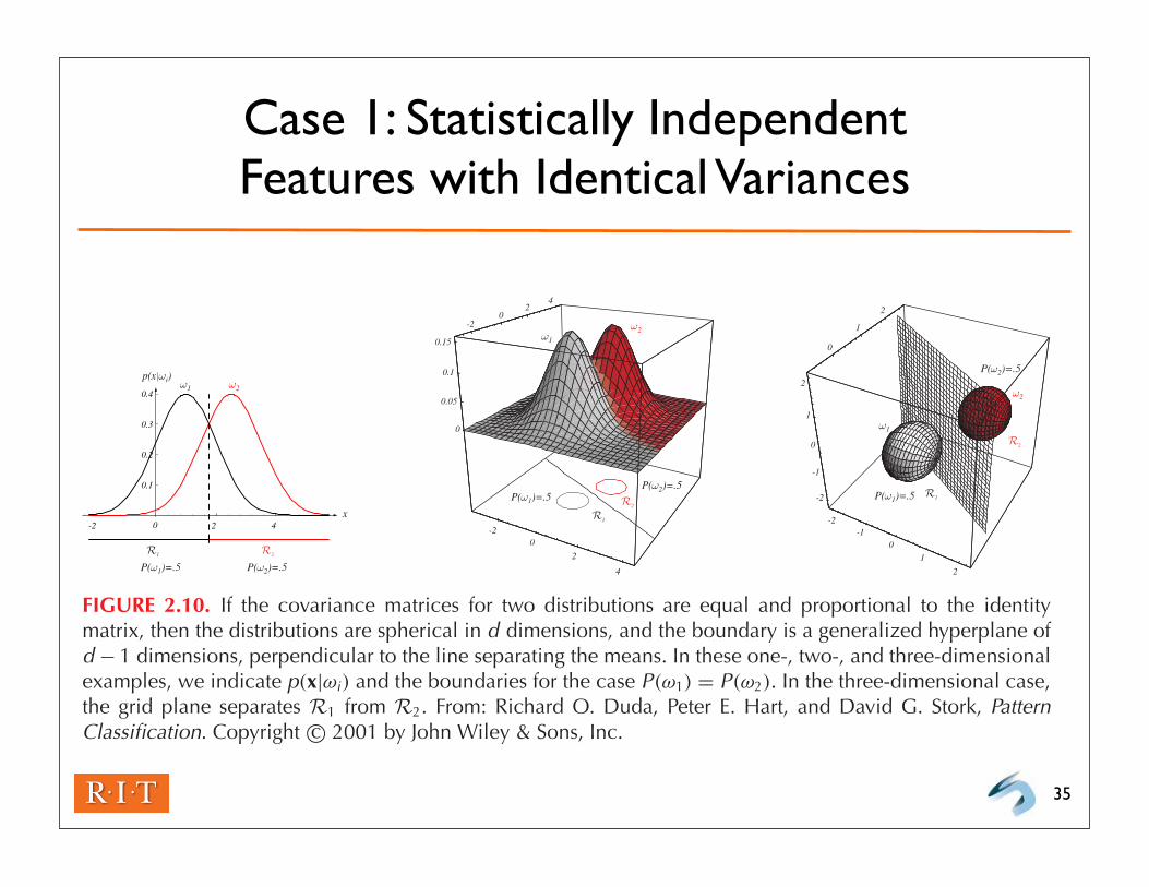
Case 1: Statistically Independent Features with Identical Variances
35
-2 2 4
0.1
0.2
0.3
0.4
P(ω1)=.5 P(ω2)=.5
x
p(x|ωi) ω1 ω2
0
R1 R2
02
4
0
0.05
0.1
0.15
-2
P(ω1)=.5P(ω2)=.5
ω1
ω2
R1
R2
-20
2
4
-2-1
01
2
0
1
2
-2
-1
0
1
2
P(ω1)=.5
P(ω2)=.5
ω1
ω2
R1
R2
FIGURE 2.10. If the covariance matrices for two distributions are equal and proportional to the identitymatrix, then the distributions are spherical in d dimensions, and the boundary is a generalized hyperplane ofd − 1 dimensions, perpendicular to the line separating the means. In these one-, two-, and three-dimensionalexamples, we indicate p(x|ωi) and the boundaries for the case P(ω1) = P(ω2). In the three-dimensional case,the grid plane separates R1 from R2. From: Richard O. Duda, Peter E. Hart, and David G. Stork, PatternClassification. Copyright c© 2001 by John Wiley & Sons, Inc.
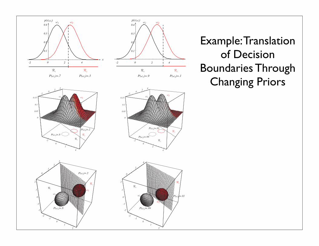
P(ω1)=.7 P(ω2)=.3
ω1 ω2
R1 R2
p(x|ωi)
x-2 2 4
0.1
0.2
0.3
0.4
0
P(ω1)=.9 P(ω2)=.1
ω1 ω2
R1 R2
p(x|ωi)
x-2 2 4
0.1
0.2
0.3
0.4
0
-2
02
4
-20
24
0
0.05
0.1
0.15
P(ω1)=.8
P(ω2)=.2
ω1 ω2
R1
R2
-2
02
4
-20
24
0
0.05
0.1
0.15
P(ω1)=.99
P(ω2)=.01
ω1ω2
R1
R2
-10
1
2
0
1
2
3
-2
-1
0
1
2
-2
P(ω1)=.8
P(ω2)=.2
ω1
ω2R1
R2
0
2
4
-10
1
2
-2
-1
0
1
2
-2
P(ω1)=.99
P(ω2)=.01ω1
ω2
R1
R2
FIGURE 2.11. As the priors are changed, the decision boundary shifts; for sufficientlydisparate priors the boundary will not lie between the means of these one-, two- andthree-dimensional spherical Gaussian distributions. From: Richard O. Duda, Peter E.Hart, and David G. Stork, Pattern Classification. Copyright c© 2001 by John Wiley &Sons, Inc.
Example: Translation of Decision
Boundaries Through Changing Priors
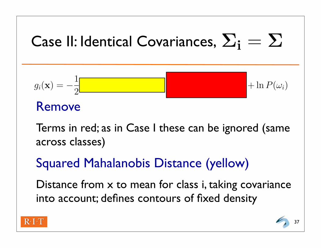
Case II: Identical Covariances,
37
Remove
Terms in red; as in Case I these can be ignored (same across classes)
Squared Mahalanobis Distance (yellow)
Distance from x to mean for class i, taking covariance into account; defines contours of fixed density
2 Case II
Σi = Σ
3 Case III
Σi = (arbitrary gaussian)
2
1 Bayes Dec. Rules: Case I
p(x|ωi) ∼ N(ωi,Σi)
gi(x) = −1
2(x− µi)
tΣi−1(x− µi)−
d
2ln 2π− 1
2ln |Σi| + ln P (ωi)
2 Case II
3 Case III
1

Case II: Identical Covariances,
Expansion of squared Mahalanobis distance
the last step comes from symmetry of the covariance matrix and thus its inverse:
Once again, term above in red is an additive constant independent of class, and can be removed
38
2 Case II
Σi = Σ
3 Case III
Σi = (arbitrary gaussian)
2
2 Case II
gi(x) = −1
2(x−µi)
tΣ−1(x−µi)+ln P (ωi)
Σi = Σ
3 Case III
Σi = (arbitrary gaussian)
2
2 Case II
gi(x) = −1
2(x−µi)
tΣ−1(x−µi)+ln P (ωi)
Σi = Σ
xtΣ−1x− xtΣ−1µi− µtiΣ−1x + µt
iΣ−1µi
= xtΣ−1x− 2(Σ−1µi)tx + µt
iΣ−1µi
3 Case III
Σi = (arbitrary gaussian)
2
2 Case II
gi(x) = −1
2(x−µi)
tΣ−1(x−µi)+ln P (ωi)
Σi = Σ
= xtΣ−1x− xtΣ−1µi− µtiΣ−1x + µt
iΣ−1µi
= xtΣ−1x− 2(Σ−1µi)tx + µt
iΣ−1µi
3 Case III
Σi = (arbitrary gaussian)
2
2 Case II
gi(x) = −1
2(x−µi)
tΣ−1(x−µi)+ln P (ωi)
Σi = Σ
= xtΣ−1x− xtΣ−1µi− µtiΣ−1x + µt
iΣ−1µi
= xtΣ−1x− 2(Σ−1µi)tx + µt
iΣ−1µi
Σt = Σ, (Σ−1)t = Σ−1
3 Case III
Σi = (arbitrary gaussian)
2
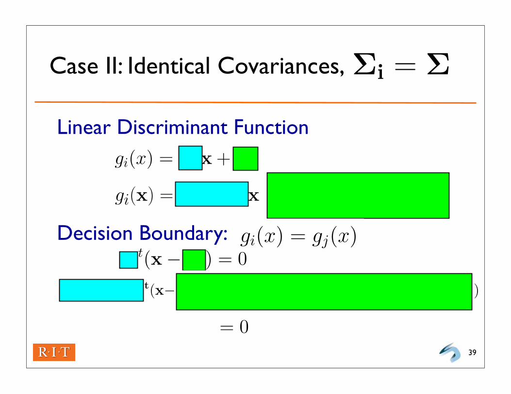
Case II: Identical Covariances,
Linear Discriminant Function
Decision Boundary:
39
1 Bayes Dec. Rules: Case I
p(x|ωi) ∼ N(ωi,Σi)
gi(x) = −1
2(x− µi)
tΣi−1(x− µi)−
d
2ln 2π− 1
2ln |Σi| + ln P (ωi)
Σi = σ2I
|Σi| = σ2d,Σ−1i = (1/σ2)I
gi(x) = −(x− µi)t(x− µi)
2σ2 + ln P (ωi)
gi(x) = − 1
2σ2 [xtx− 2µt
ix + µitµi] + ln P (ωi)
gi(x) =1
σ2µix−1
2σ2µtiµi + ln P (ωi)
gi(x) = wtix + ωi0
1
2 Case II
gi(x) = −1
2(x−µi)
tΣ−1(x−µi)+ln P (ωi)
Σi = Σ
= xtΣ−1x− xtΣ−1µi− µtiΣ−1x + µt
iΣ−1µi
= xtΣ−1x− 2(Σ−1µi)tx + µt
iΣ−1µi
Σt = Σ, (Σ−1)t = Σ−1
gi(x) = (Σ−1µi)tx −1
2µt
iΣ−1µi + ln P (ωi)
3 Case III
Σi = (arbitrary gaussian)
2
2 Case II
Σi = Σ
3 Case III
Σi = (arbitrary gaussian)
2
1 Bayes Dec. Rules: Case I
p(x|ωi) ∼ N(ωi,Σi)
gi(x) = −1
2(x− µi)
tΣi−1(x− µi)−
d
2ln 2π− 1
2ln |Σi| + ln P (ωi)
Σi = σ2I
|Σi| = σ2d,Σ−1i = (1/σ2)I
gi(x) = −(x− µi)t(x− µi)
2σ2 + ln P (ωi)
gi(x) = − 1
2σ2 [xtx− 2µt
ix + µitµi] + ln P (ωi)
gi(x) =1
σ2µitx− 1
2σ2µtiµi + ln P (ωi)
gi(x) = wtix + ωi0
gi(x) = gj(x)
1
1 Bayes Dec. Rules: Case I
p(x|ωi) ∼ N(ωi,Σi)
gi(x) = −1
2(x− µi)
tΣi−1(x− µi)−
d
2ln 2π− 1
2ln |Σi| + ln P (ωi)
Σi = σ2I
|Σi| = σ2d,Σ−1i = (1/σ2)I
gi(x) = −(x− µi)t(x− µi)
2σ2 + ln P (ωi)
gi(x) = − 1
2σ2 [xtx− 2µt
ix + µitµi] + ln P (ωi)
gi(x) =1
σ2µitx− 1
2σ2µtiµi + ln P (ωi)
gi(x) = wtix + ωi0
gi(x) = gj(x)
wt(x− x0) = 0
1
2 Case II
gi(x) = −1
2(x− µi)
tΣ−1(x− µi) + ln P (ωi)
Σi = Σ
= xtΣ−1x − xtΣ−1µi − µtiΣ
−1x + µtiΣ
−1µi
= xtΣ−1x − 2(Σ−1µi)tx + µt
iΣ−1µi
Σt = Σ, (Σ−1)t = Σ−1
gi(x) = (Σ−1µi)tx − 1
2µt
iΣ−1µi + ln P (ωi)
(Σ−1(µi−µj))t(x−
(1
2(µi + µj)−
ln[P(ωi)/Pωj)
(µi − µj)Σ−1(µi − µj)(µi − µj)
))
3 Case III
Σi = (arbitrary gaussian)
2
2 Case II
gi(x) = −1
2(x− µi)
tΣ−1(x− µi) + ln P (ωi)
Σi = Σ
= xtΣ−1x − xtΣ−1µi − µtiΣ
−1x + µtiΣ
−1µi
= xtΣ−1x − 2(Σ−1µi)tx + µt
iΣ−1µi
Σt = Σ, (Σ−1)t = Σ−1
gi(x) = (Σ−1µi)tx − 1
2µt
iΣ−1µi + ln P (ωi)
(Σ−1(µi−µj))t(x−
(1
2(µi + µj)−
ln[P(ωi)/Pωj)
(µi − µj)Σ−1(µi − µj)(µi − µj)
))
= 0
3 Case III
Σi = (arbitrary gaussian)
2
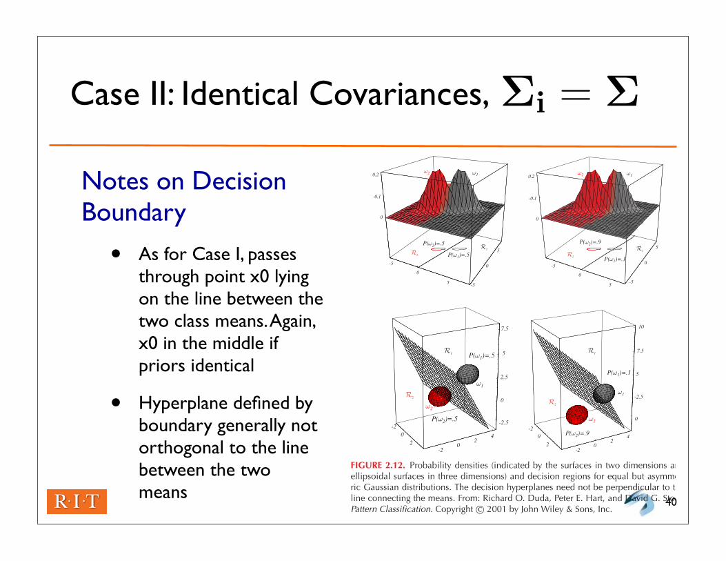
Case II: Identical Covariances,
Notes on Decision Boundary
• As for Case I, passes through point x0 lying on the line between the two class means. Again, x0 in the middle if priors identical
• Hyperplane defined by boundary generally not orthogonal to the line between the two means
40
2 Case II
Σi = Σ
3 Case III
Σi = (arbitrary gaussian)
2
-5
0
5 -5
0
5
0
-0.1
0.2
P(ω1)=.5
P(ω2)=.5
ω1ω2
R1R2
-5
0
5-5
0
5
0
-0.1
0.2
P(ω1)=.1
P(ω2)=.9
ω1ω2
R1R2
-20
2-2
02
4
-2.5
0
2.5
5
7.5
P(ω1)=.5
P(ω2)=.5
ω1
ω2
R1
R2
-20
2-2
02
4
0
-2.5
5
7.5
10
P(ω1)=.1
P(ω2)=.9
ω1
ω2
R1
R2
FIGURE 2.12. Probability densities (indicated by the surfaces in two dimensions andellipsoidal surfaces in three dimensions) and decision regions for equal but asymmet-ric Gaussian distributions. The decision hyperplanes need not be perpendicular to theline connecting the means. From: Richard O. Duda, Peter E. Hart, and David G. Stork,Pattern Classification. Copyright c© 2001 by John Wiley & Sons, Inc.
Case III: arbitrary
41
2 Case II
gi(x) = −1
2(x− µi)
tΣ−1(x− µi) + ln P (ωi)
Σi = Σ
= xtΣ−1x − xtΣ−1µi − µtiΣ
−1x + µtiΣ
−1µi
= xtΣ−1x − 2(Σ−1µi)tx + µt
iΣ−1µi
Σt = Σ, (Σ−1)t = Σ−1
gi(x) = (Σ−1µi)tx − 1
2µt
iΣ−1µi + ln P (ωi)
(Σ−1(µi−µj))t(x−
(1
2(µi + µj)−
ln[P(ωi)/Pωj)
(µi − µj)Σ−1(µi − µj)(µi − µj)
))
= 0
3 Case III
Σi = (arbitrary gaussian)
2
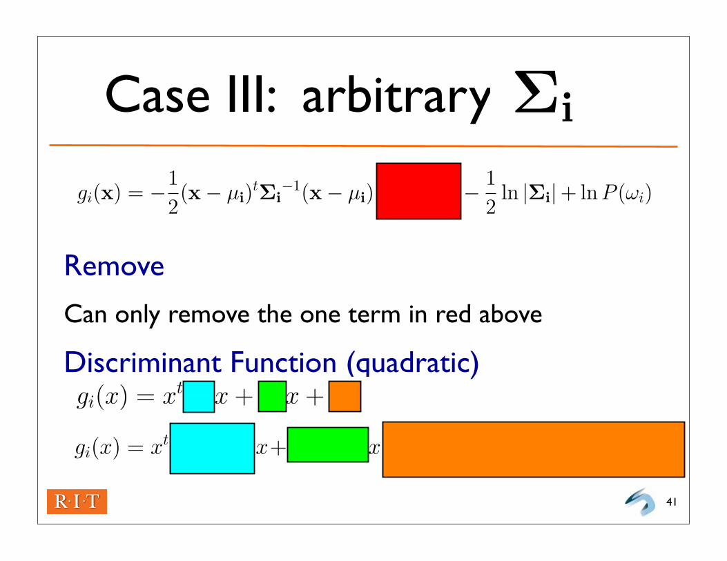
Remove
Can only remove the one term in red above
Discriminant Function (quadratic)
1 Bayes Dec. Rules: Case I
p(x|ωi) ∼ N(ωi,Σi)
gi(x) = −1
2(x− µi)
tΣi−1(x− µi)−
d
2ln 2π− 1
2ln |Σi| + ln P (ωi)
2 Case II
3 Case III
1
3 Case III
Σi = (arbitrary gaussian)
gi(x) = xtWix + wtix + ωi0
gi(x) = xt(−1
2Σ−1
i )x+(Σ−1i µi)x−
1
2µt
iΣ−1i µi−
1
2ln |Σi|+ln P (ωi)
3
3 Case III
Σi = (arbitrary gaussian)
gi(x) = xtWix + wtix + ωi0
gi(x) = xt(−1
2Σ−1
i )x+(Σ−1i µi)
tx− 1
2µt
iΣ−1i µi−
1
2ln |Σi|+ln P (ωi)
3
Case III: arbitrary
Decision Boundaries
Are hyperquadrics: can be hyperplanes, hyperplane pairs, hyperspheres, hyperellipsoids, hyperparabaloids, hyperhyperparabaloids
Decision Regions
Need not be simply connected, even in one dimension (next slide)
42
2 Case II
gi(x) = −1
2(x− µi)
tΣ−1(x− µi) + ln P (ωi)
Σi = Σ
= xtΣ−1x − xtΣ−1µi − µtiΣ
−1x + µtiΣ
−1µi
= xtΣ−1x − 2(Σ−1µi)tx + µt
iΣ−1µi
Σt = Σ, (Σ−1)t = Σ−1
gi(x) = (Σ−1µi)tx − 1
2µt
iΣ−1µi + ln P (ωi)
(Σ−1(µi−µj))t(x−
(1
2(µi + µj)−
ln[P(ωi)/Pωj)
(µi − µj)Σ−1(µi − µj)(µi − µj)
))
= 0
3 Case III
Σi = (arbitrary gaussian)
2

Case 3: Arbitrary Covariances
43
-5 -2.5 2.5 5 7.5
0.1
0.2
0.3
0.4
x
p(x|ωi)
ω1
ω2
R1 R2 R1
FIGURE 2.13. Non-simply connected decision regions can arise in one dimensions forGaussians having unequal variance. From: Richard O. Duda, Peter E. Hart, and DavidG. Stork, Pattern Classification. Copyright c© 2001 by John Wiley & Sons, Inc.
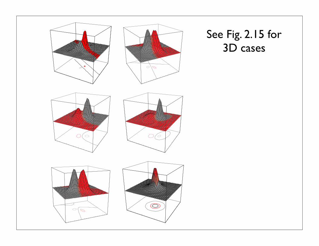
FIGURE 2.14. Arbitrary Gaussian distributions lead to Bayes decision boundaries thatare general hyperquadrics. Conversely, given any hyperquadric, one can find two Gaus-sian distributions whose Bayes decision boundary is that hyperquadric. These variancesare indicated by the contours of constant probability density. From: Richard O. Duda,Peter E. Hart, and David G. Stork, Pattern Classification. Copyright c© 2001 by JohnWiley & Sons, Inc.
See Fig. 2.15 for 3D cases
R3
R2
R1
R4
R4
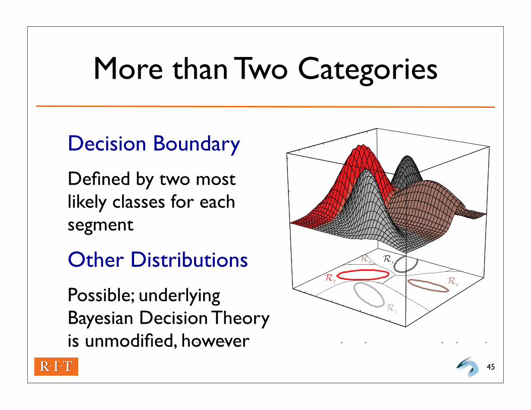
FIGURE 2.16. The decision regions for four normal distributions. Even with such a lownumber of categories, the shapes of the boundary regions can be rather complex. From:Richard O. Duda, Peter E. Hart, and David G. Stork, Pattern Classification. Copyrightc© 2001 by John Wiley & Sons, Inc.
More than Two Categories
45
Decision Boundary
Defined by two most likely classes for each segment
Other Distributions
Possible; underlying Bayesian Decision Theory is unmodified, however
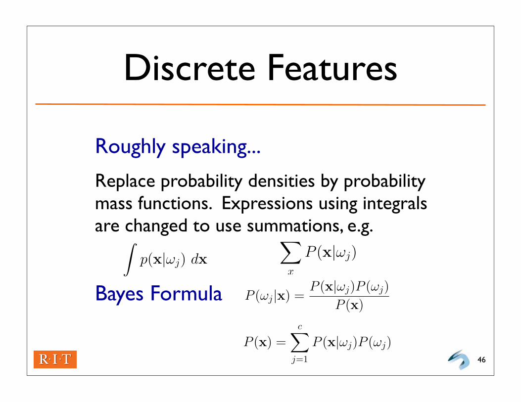
Discrete Features
Roughly speaking...
Replace probability densities by probability mass functions. Expressions using integrals are changed to use summations, e.g.
Bayes Formula
46
∫p(x|ωj) dx
∑
x
P (x|ωj)
4
∫p(x|ωj) dx
∑
x
P (x|ωj)
4
∫p(x|ωj) dx
∑
x
P (x|ωj)
P (ωj|x) =P (x|ωj)P (ωj)
P (x)
P (x) =c∑
j=1
P (x|ωj)P (ωj)
4
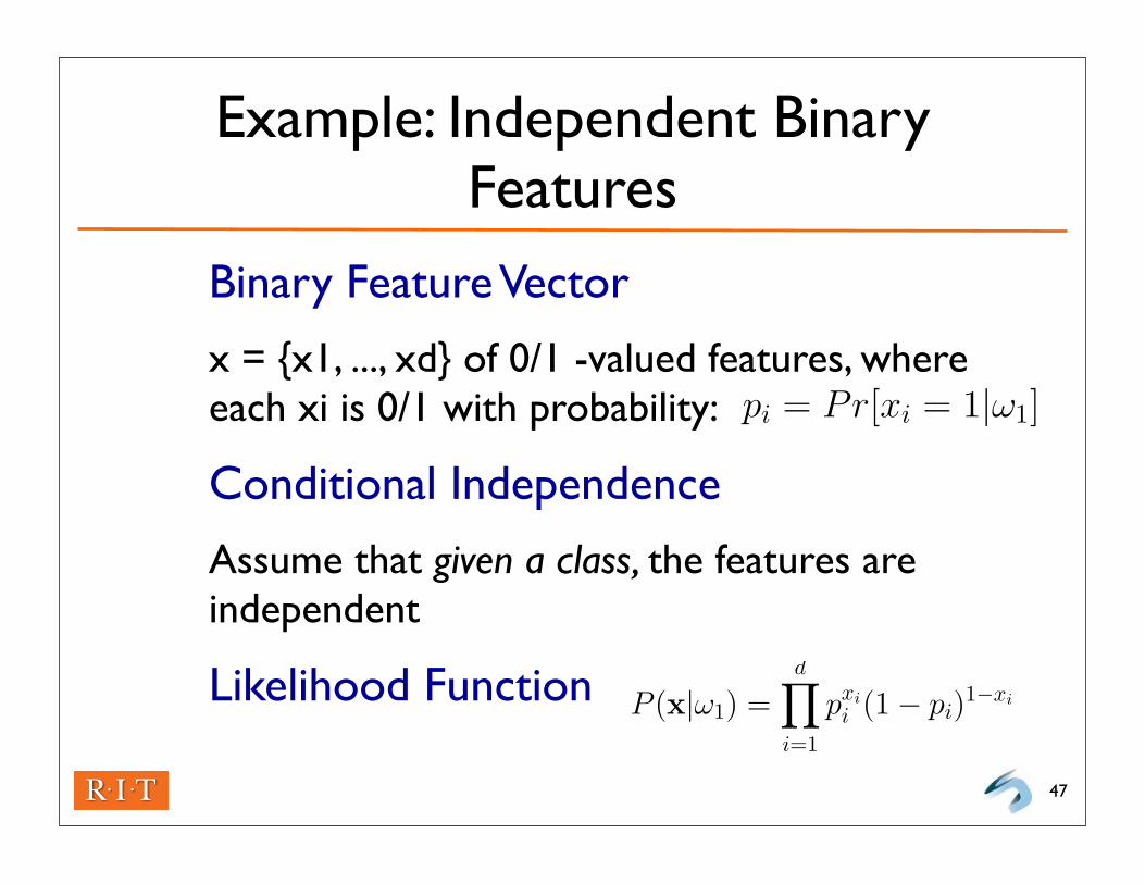
Example: Independent Binary Features
Binary Feature Vector
x = {x1, ..., xd} of 0/1 -valued features, where each xi is 0/1 with probability:
Conditional Independence
Assume that given a class, the features are independent
Likelihood Function
47
∫p(x|ωj) dx
∑
x
P (x|ωj)
P (ωj|x) =P (x|ωj)P (ωj)
P (x)
P (x) =c∑
j=1
P (x|ωj)P (ωj)
pi = Pr[xi = 1|ω1]
4
∫p(x|ωj) dx
∑
x
P (x|ωj)
P (ωj|x) =P (x|ωj)P (ωj)
P (x)
P (x) =c∑
j=1
P (x|ωj)P (ωj)
pi = Pr[xi = 1|ω1]
P (x|ω1) =d∏
i=1
pxii (1− pi)
1−xi
4