bayesiannetworks - github pages

Bayesian Networks

David Rosenberg

New York University

October 29, 2016

David Rosenberg (New York University) DS-GA 1003 October 29, 2016 1 / 38

Introduction

Introduction


Introduction

Probabilistic Reasoning

Represent system of interest by a set of random variables

(X1, . . . ,Xd) .

Suppose by research or ML, we get a joint probability distribution

p(x1, . . . ,xd).

We’d like to be able to do “inference” on this model – essentially,answer queries:

1 What is the most likely of value X1?2 What is the most likely of value X1, given we’ve observed X2 = 1?3 Distribution of (X1,X2) given observation of (X3 = x3, . . . ,Xd = xd )?


Introduction

Example: Medical Diagnosis

Variables for each symptomfever, cough, fast breathing, shaking, nausea, vomiting

Variables for each diseasepneumonia, flu, common cold, bronchitis, tuberculosis

Diagnosis is performed by inference in the model:

p(pneumonia= 1 | cough= 1, fever= 1,vomiting= 0)

The QMR-DT (Quick Medical Reference - Decision Theoretic) has

600 diseases4000 symptoms

Example from David Sontag’s Inference and Representation, Lecture 1.


Discrete Probability Distribution Review




Some Notation

This lecture we’ll only be considering discrete random variables.Capital letters X1, . . . ,Xd ,Y , etc. denote random variables.Lower case letters x1, . . . ,xn,y denote the values taken.Probability that X1 = x1 and X2 = x2 will be denoted

P(X1 = x1,X2 = x2) .

We’ll generally write things in terms of the probability mass function:

p(x1,x2, . . . ,xd) := P(X1 = x1,X2 = x2, . . . ,Xd = xd)



Representing Probability Distributions

Let’s consider the case of discrete random variables.Conceptually, everything can be represented with probability tables.Variables

Temperature T ∈ {hot,cold}Weather W ∈ {sun, rain}

t p(t)

hot 0.5cold 0.5

w p(w)

sun 0.6rain 0.4

These are the marginal probability distributions.To do reasoning, we need the joint probability distribution.

Based on David Sontag’s DS-GA 1003 Lectures, Spring 2014, Lecture 10.



Joint Probability Distributions

A joint probability distribution for T and W is given by

t w p(t,w)

hot sun 0.4hot rain 0.1cold sun 0.2cold rain 0.3

With the joint we can answer question such as

p(sun | hot)=?p(rain | cold)=?

Based on David Sontag’s DS-GA 1003 Lectures, Spring 2014, Lecture 10.



Representing Joint Distributions

Consider random variables X1, . . . ,Xd ∈ {0,1}.How many parameters do we need to represent the joint distribution?Joint probability table has 2d rows.For QMR-DT, that’s 24600 > 101000 rows.That’s not going to happen.Only ∼ 1080 atoms in the universe.Having exponentially many parameters is a problem for

storagecomputation (inference is summing over exponentially many rows)statistical estimation / learning



How to Restrict the Complexity?

Restrict the space of probability distributionsWe will make various independence assumptions.Extreme assumption: X1, . . . ,Xd are mutually independent.

DefinitionDiscrete random variables X1, . . . ,Xd are mutually independent if theirjoint probability mass function (PMF) factorizes as

p(x1,x2, . . . ,xd) = p(x1)p(x2) · · ·p(xd).

Note: We usually just write independent for “mutually independent”.How many parameters to represent the joint distribution, assumingindependence?



Assume Full Independence

How many parameters to represent the joint distribution?Say p(Xi = 1) = θi , for i = 1, . . . ,d .Clever representation: Since xi ∈ {0,1}, we can write

P(Xi = xi ) = θxii (1−θi )

1−xi .

Then by independence,

p(x1, . . . ,xd) =d∏

i=1

θxii (1−θi )1−xi

How many parameters?d parameters needed to represent the joint.



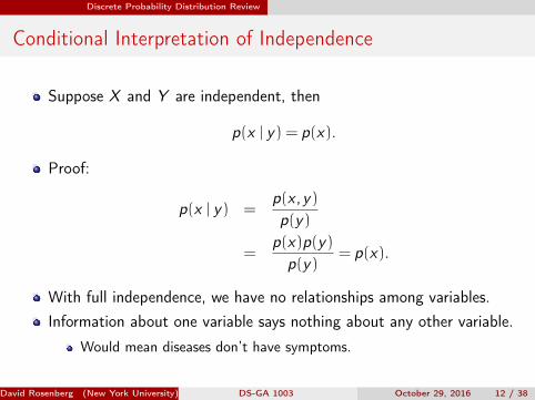
Conditional Interpretation of Independence

Suppose X and Y are independent, then

p(x | y) = p(x).

Proof:

p(x | y) =p(x ,y)

p(y)

=p(x)p(y)

p(y)= p(x).

With full independence, we have no relationships among variables.Information about one variable says nothing about any other variable.

Would mean diseases don’t have symptoms.



Conditional Independence

Consider 3 events:1 W = {The grass is wet}2 S = {The road is slippery}3 R = {It’s raining}

These events are certainly not independent.Raining (R) =⇒ Grass is wet AND The road is slippery (W ∩S)Grass is wet (W ) =⇒ More likely that the road is slippery (S)

Suppose we know that it’s raining.Then, we learn that the grass is wet.Does this tell us anything new about whether the road is slippery?

Once we know R , then W and S become independent.This is called conditional independence, and we’ll denote it as

W ⊥ S | R.



Conditional Independence

DefinitionWe say W and S are conditionally independent given R , denoted

W ⊥ S | R,

if the conditional joint factorizes as

p(w ,s | r) = p(w | r)p(s | r).

Also holds when W , S , and R represent sets of random variables.

Can have conditional independence without independence.

Can have independence without conditional independence.



Example: Rainy, Slippery, Wet

Consider 3 events:1 W = {The grass is wet}2 S = {The road is slippery}3 R = {It’s raining}

Represent joint distribution as

p(w ,s, r) = p(w ,s | r)p(r) (no assumptions so far)= p(w | r)p(s | r)p(r) (assuming W ⊥ S | R)

How many parameters to specify the joint?p(w | r) requires two parameters: one for r = 1 and one for r = 0.p(s | r) requires two.p(r) requires one parameter,

Full joint: 7 parameters. Conditional independence: 5 parameters.Full independence: 3 parameters.


Bayesian Networks

Bayesian Networks


Bayesian Networks

Bayesian Networks: Introduction

Bayesian Networks are

used to specify joint probability distributions thathave a particular factorization.

p(c ,h,a, i) = p(c)p(a)

×p(h | c,a)p(i | a)

With practice, one can read conditional independence relationshipsdirectly from the graph.

From Percy Liang’s "Lecture 14: Bayesian networks II" slides from Stanford’s CS221, Autumn 2014.


Bayesian Networks

Directed Graphs

A directed graph is a pair G = (V,E) , whereV= {1, . . . ,d} is a set of nodes andE= {(s, t) | s, t ∈ V} is a set of directed edges.

4 5

2 3

1

Parents(5) = {3}Parents(4) = {2,3}Children(3) = {4,5}

Descendants(1) = {2,3,4,5}NonDescendants(3) = {1,2}

KPM Figure 10.2(a).


Bayesian Networks

Directed Acyclic Graphs (DAGs)

A DAG is a directed graph with no directed cycles.

DAG

4 5

2 3

1

Not a DAG

Every DAG has a topological ordering, in which parents have lowernumbers than their children.

http://www.geeksforgeeks.org/wp-content/uploads/SCC1.png and KPM Figure 10.2(a).


Bayesian Networks

Bayesian Networks

DefinitionA Bayesian network is a

DAG G = (V,E), where V= {1, . . . ,d}, anda corresponding set of random variables X = {X1, . . . ,Xd }

wherethe joint probability distribution over X factorizes as

p(x1, . . . ,xd) =d∏

i=1

p(xi | xParents(i)).

Bayesian networks are also known asdirected graphical models, andbelief networks.


Conditional Independencies




Bayesian Networks: “A Common Cause”

c

a b

p(a,b,c) = p(c)p(a | c)p(b | c)

Are a and b independent? (c=Rain, a=Slippery, b=Wet?)

p(a,b) =∑c

p(c)p(a | c)p(b | c),

which in general will not be equal to p(a)p(b).

From Bishop’s Pattern recognition and machine learning, Figure 8.15.



Bayesian Networks: “An Indirect Effect”

a c b

p(a,b,c) = p(a)p(c | a)p(b | c)

Are a and b independent? (Note: This is a Markov chain)(e.g. a=raining, c=wet ground, b=mud on shoes)

p(a,b) =∑c

p(a,b,c)

= p(a)∑c

p(c | a)p(b | c)

So doesn’t factorize, thus not independent, in general.




Bayesian Networks: “An Indirect Effect”

a c b

p(a,b,c) = p(a)p(c | a)p(b | c)

Are a and b independent after observing c?(e.g. a=raining, c=wet ground, b=mud on shoes)

p(a,b | c) = p(a,b,c)/p(c)

= p(a)p(c | a)p(b | c)/p(c)

= p(a | c)p(b | c)

So a⊥ b | c .




Bayesian Networks: “A Common Effect”

c

a b

p(a,b,c) = p(a)p(b)p(c | a,b)Are a and b independent? (a=course difficulty, b=knowledge, c= grade)

p(a,b) =∑c

p(a)p(b)p(c | a,b)

= p(a)p(b)∑c

p(c | a,b)

= p(a)p(b)

So a⊥ b.




Bayesian Networks: “A Common Effect” or “V-Structure”

c

a b

p(a,b,c) = p(a)p(b)p(c | a,b)

Are a and b independent, given observation of c? (a=course difficulty,b=knowledge, c= grade)

p(a,b | c) = p(a)p(b)p(c | a,b)/p(c)

which does not factorize into p(a | c)p(b | c), in general.




Conditional Independence from Graph Structure

In general, given 3 sets of nodes A, B , and C

How can we determine whether

A⊥ B | C?

There is a purely graph-theoretic notion of “d-separation” that isequivalent to conditional independence.Suppose we have observed C and we want to do inference on A.We could ignore any evidence collected about B , where A⊥ B | C .See KPM Section 10.5.1 for details.



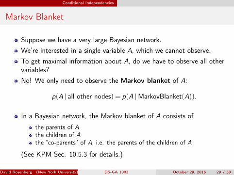
Markov Blanket

Suppose we have a very large Bayesian network.We’re interested in a single variable A, which we cannot observe.To get maximal information about A, do we have to observe all othervariables?No! We only need to observe the Markov blanket of A:

p(A | all other nodes) = p(A |MarkovBlanket(A)).

In a Bayesian network, the Markov blanket of A consists of

the parents of Athe children of Athe “co-parents” of A, i.e. the parents of the children of A

(See KPM Sec. 10.5.3 for details.)



Markov Blanket

Markov Blanket of A in a Bayesian Network:

From http://en.wikipedia.org/wiki/Markov_blanket: "Diagram of a Markov blanket" by Laughsinthestocks -Licensed under CC0 via Wikimedia Commons


http://en.wikipedia.org/wiki/Markov_blanket

When to use Bayesian Networks?




Bayesian Networks

Bayesian Networks are great when

you know something about the relationships between your variables, oryou will routinely need to make inferences with incomplete data.

Challenges:

The naive approach to inference doesn’t work beyond small scale.Need more sophisticated algorithm:

exact inferenceapproximate inference


Naive Bayes

Naive Bayes


Naive Bayes

Binary Naive Bayes: A Generative Model for Classification

X={(

X1,X2,X3,X4) ∈ {0,1}4)}

Y= {0,1} be a class label.

Consider the Bayesian network depicted below:

Y

X1 X2 X3 X4

BN structure implies joint distribution factors as:

p(x1,x2,x3,x4,y) = p(y)p(x1 | y)p(x2 | y)p(x3 | y)p(x4 | y)

Features X1, . . . ,X4 are independent given the class label Y .KPM Figure 10.2(a).


Markov Models

Markov Models


Markov Models

Markov Chain Model

A Markov chain model has structure:

x1 x2 x3

· · ·

p(x1,x2,x3, . . .) = p(x1)p(x2 | x1)p(x3 | x2) · · ·

Conditional distributions p(xi | xi−1) is called the transition model.When conditional distribution independent of i , calledtime-homogeneous.4-state transition model for Xi ∈ {S1,S2,S3,S4}:

S1

0.3 0.5

0.7 0.4 0.5

0.6

0.9

0.1

S2 S3 S4

KPM Figure 10.3(a) and Koller and Friedman’s Probabilistic Graphical Models Figure 6.04.


Markov Models

Hidden Markov Model

A hidden Markov model (HMM) has structure:

x1 x2 xT

z1 z2 zT

p(x1,z1,x2,z2,x3,z3, . . .) = p(z1)T∏

t=2

p(zt | zt−1)︸︷︷︸Transition Model

T∏t=1

p(xt | zt)︸︷︷︸Observation Model

At deployment time, we typically only observe X1, . . . ,XT .Want to infer Z1, . . . ,ZT .e.g. Want to most likely sequence (Z1, . . . ,ZT ) . (Use Viterbialgorithm.)

KPM Figure 10.4


Markov Models

Maximum Entropy Markov Model

A maximum entropy Markov model (MEMM) has structure:

p(y1 . . . ,y5 | x) = p(y0)

5∏t=1

p(yt | yt−1,x)︸︷︷︸Conditional Transition Model

At deployment time, we only observe X1, . . . ,XT .This is a conditional model. (And not a generative model).

Koller and Friedman’s Probabilistic Graphical Models Figure 20.A.1.


bayesiannetworks - github pages

Documents