becin 002 chapter 1 -...

Chapter 1Chapter 1

The Nature of Applied

Econometrics

1

Section 1.1Section 1.1

What Is Applied

Econometrics?

2

Applied Econometrics� Applied econometrics deals with the measurement of

business, economic, or financial relationships.“The study of the application of statistical methods to the analysis of economic phenomena.” (Tintner 1953) � Business analysts often need to be in position to do

the following:– interpret the economic landscape– identify and assess the influence of several

exogenous or predetermined factors on one or more endogenous variables

– provide ex-ante forecasts of one or more endogenous variables

How do you achieve these objectives?

33

Why Do Business Analysts Want to Achieve These Objectives?To improve decision making!Example: Investigate key determinants of demand

for Prego spaghetti sauce:� price of Prego� price of competitors (Ragu, Classico, Hunt’s, � price of competitors (Ragu, Classico, Hunt’s,

Newman’s Own)� in-store displays� coupons� price of pasta

Forecast sales of Prego spaghetti sauce one month, one quarter, or even one year into the future.

44


Course of Action –Development of Formal Quantitative Models

5

Basic Approaches To Model Building� Intuitive approach� Bayesian models (to bridge the gap between intuitive

models (prior beliefs) and more formal statistical models)

� Time-Series approach� Structural (Econometric) approach� Structural (Econometric) approach

66


Disciplines in Applied

Econometrics

7

Disciplines in Applied Econometrics� Economics, mathematics, and statistics are combined.� Economic theory establishes the boundaries of the

questions you can address.� Empirical models are associated with some sort of

mathematical representation.� Derivatives are the cornerstones of the calculation of � Derivatives are the cornerstones of the calculation of

marginal effects.� Statistics provide the vehicle for making inductive

inferences from a sample to a population.� Little opportunity exists for controlled experiments.� Econometrics emphasizes the importance of Monte

Carlo simulation as an alternative to controlled experiments.

88


Empirical Models and

Modeling Approaches

9

Empirical Models� At the heart of applied econometrics lies the

development of empirical models.� Empirical models are nothing more than parsimonious

representations of reality.� Empirical models indigenous to applied econometrics

are stochastic, not deterministic.� The purpose is to model the behavior of agents such

as consumers, firms, banks, and the stock market, all of which have in common the human element.

� Empirical models can be single-equation or multi-equation specifications.

� Empirical models can be linear or nonlinear in parameters.

1010

Econometric (Structural)

ModelsTime-Series

Models

Intuitive Models

Single-Equation

Univariate MultivariateUnivariate

Modeling Approaches

Multi-Equation

1111

Equation

Trend Extrapolation Models

Box-Jenkins ARIMA Models

Error Correction

Models

Vector Autoregression (VAR) Models

Recursive Models

Simultaneous Models

Seemingly Unrelated Regression Models

Equation

In some instances, econometric models might encompass elements of time-series models (for example, ARCH and GARCH models, adjustments for serial correlation).

Seasonal Models

Smoothing Models

Model SpecificationModel specification is driven by the following:� Data (number of observations)� Data (number of variables)� Theoretical Considerations� Atheoretical Considerations� Dynamics� Dynamics� Experience� Question(s) Addressed

1212

Intuitive ApproachThe basic premise is that any data series (typically a data series that varies over time) can be decomposed into a trend component, a seasonal component, a cyclical component, and a random component. This decomposition can either be additive or multiplicative. This approach only deals with a single data series and, as such, is univariate in nature.such, is univariate in nature.

With the intuitive approach, analysts focus on models designed to capture trends, seasonal movements, and cyclical patterns.

Time series models also capture these components but in a more sophisticated fashion.

1313

Time-Series Approach� ARIMA models – Univariate approach� Vector autoregression models – Multivariate approach� Causality tests� Impulse response functions� Cointegration� Error correction models – Multivariate approach� Error correction models – Multivariate approach� Other models (for example, ARCH and GARCH

models)

1414

Structural or Econometric Approach� Single-equation specifications – Multivariate approach� Multi-equation specifications – Multivariate approach� Interpretation of coefficients� Tests of hypotheses

1515

Applied EconometricsSimply put, applied econometrics entails the following:� unification of economics, mathematics, and statistics� measurement of business, economic, or financial

relationships� measurement of underlying relationships for the

purpose of testing and developing economic theory purpose of testing and developing economic theory (a form of data mining)

1616


Components of Applied

Econometrics

17

Components of Applied EconometricsApplied econometrics involves four phases of analysis:� Specification – the model-building activity� Estimation – fitting the model to data� Verification – testing the model� Prediction – producing ex-ante forecasts and

conducting ex-post forecast evaluationsconducting ex-post forecast evaluations

1818

Components of Applied

Specification Estimation

19

Components of Applied Econometrics

Verification Prediction

19

The Translation of Economic Models into Statistical Models� A key issue in applied econometrics is the use of proxy

variables. Proxy variables generally arise due to unavailability of appropriate data.

“Econometric theory is like an exquisitely balanced French recipe, spelling out precisely with how many turns to mix the sauce, how many carats of spice to add, and for how many sauce, how many carats of spice to add, and for how many milliseconds to bake the mixture at exactly 474 degrees of temperature. But when the statistical cook turns to raw materials, he finds that hearts of cactus fruit are unavailable, so he substitutes chunks of cantaloupe; where the recipe calls for vermicelli he uses shredded wheat; and he substitutes green garment dye for curry, ping-pong balls for turtle’s eggs, and for a vintage bottle (1883) of champagne, a can of turpentine.” (Valavanis 1959, p. 83)

2020

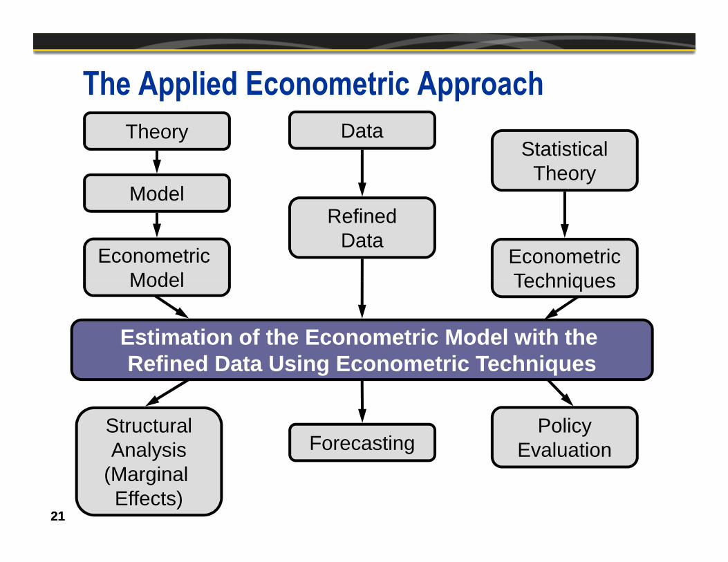
The Applied Econometric Approach

Econometric Model

Theory

Model

Data

RefinedData

StatisticalTheory

EconometricTechniques

2121

Model

Estimation of the Econometric Model with the Refined Data Using Econometric Techniques

StructuralAnalysis

(Marginal Effects)

Techniques

ForecastingPolicy

Evaluation


Products of Applied

Econometrics

22

1. Structural analysis (marginal effects)

2. Forecasting

Interrelated By-Products of

Applied Econometrics

3. Policy evaluation

2323

Econometrics

Structural Analysis and Forecasting� Structural analysis – Use of estimated econometric

models for the quantitative measurement of economic relationships

� Forecasting – Use of estimated econometric models to predict quantitative values of certain variables outside the sample of data actually observed

� Confidence or tolerance intervals of forecasts, taking into account standard errors

� Conditional versus unconditional forecasts

2424

The Structure of Applied Research

Problem Definition

TheoryEconomic TheoryStatistical Theory

Model Specification

Model Definition(variables)

Data Assembly

2525

Statistical TheoryMathematics

Previous KnowledgePrevious Research

Evaluate and Interpret Results

Descriptive Analysis

Analytical Phase

REPORT


Getting Started

26

Applied Econometrics and Model SpecificationApplied econometrics begins with model specification:� Model specification entails the expression of theoretical

constructs in mathematical terms.� This phase of applied econometrics constitutes the model

building activity.� In essence, model specification is the translation of theoretical

constructs into mathematical/statistical forms.� Fundamental principles in model building:

– The principle of parsimony (If other things are the same, simple models generally are preferable to complex models, especially in forecasting.)

– The shrinkage principle (Imposing restrictions either on estimated parameters or on forecasts often improves model performance.)

– The KISS principle (Zellner, 2001) “Keep it Sophistically Simple”

2727

Example: Estimation of Demand Relationships� Often in applied econometrics, analysts have an

interest in estimating demand relationships, particularly for commodities.

� Analysts might want to estimate the demand for cosmetic products, automobiles, various food products, or various beverages.

2828

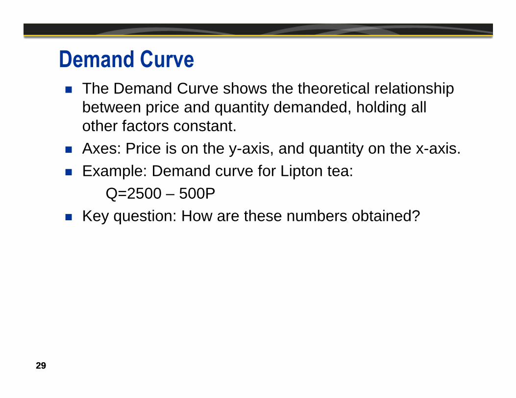
Demand Curve� The Demand Curve shows the theoretical relationship

between price and quantity demanded, holding all other factors constant.

� Axes: Price is on the y-axis, and quantity on the x-axis.� Example: Demand curve for Lipton tea:

Q=2500 – 500PQ=2500 – 500P� Key question: How are these numbers obtained?

2929

Demand Curve for Lipton TeaAverage price per package

Demand Curve

Q = 2,500 – 500P

5

4

3030

Q = 2,500 – 500P

P = 5 – .002Q3

2

1

500 1000 1500 2000 2500

Packages of Lipton tea

Own-Price Effects� Movement along a given demand curve reflects a

change in the price and quantity of the commodity in question.

� Answer the following question: What happens to the quantity demanded if the price changes (exogenously) but holds all other factors constant?Law of demand:� Law of demand:– The demand curve is negatively sloped.– An increase (a decrease) in price leads to a

decrease (an increase) in quantity demanded. – This is an important empirical finding in economics.

3131

Other Factors Affecting Demand� Prices of other products� Income� Advertising (positive information)� Food recalls or food scares (negative information)� Health and nutrition factors� Lifestyle factors� Lifestyle factors� Tastes and preferences

3232

Translations of the Theoretical Construct into a Statistical Model1. Q = a-bP2. Q = a0 – a1P + a2I + a3A + a4PS

own-price effect income effect advertising price of substitute product

� The coefficients a0, a1, a2, a3, and a4 are labeled the demand parameters.

� You expect certain signs and magnitudes of the demand parameters according to economic theory.

� Different versions of the econometric model for applied analysis are possible.

3333

own-price effect(-)

income effect(+)

advertising effect

(+)

price of substitute product(+)

Linear Regression Model Development� The starting point rests on the development of a linear

regression model.� Philosophical differences exist among statisticians and

applied econometric analysts.� Attention centered on the signs and magnitudes of the

coefficients are inherent in the model.� Model specifications in applied econometrics are non-

unique.� Model specifications provide the blueprint for action.

3434


The Generic Multiple

Regression Model

35

The Generic Multiple Regression Model

ikiki22i110i X...XXY ε+β++β+β+β=

εβ +=

=

XY

ni ,...,1

jji

i

X

Y β=∂∂

k22221

k11211

2

1

X...XX1

X...XX1

X...XX1

X

Y

Y

Y

Y

=

=MMMM

Estimation of regression parameters:� Least squares (No knowledge of the distribution of the error or disturbance terms is required.)� Maximum likelihood (requires knowledge of the distribution of the error or disturbance terms)� The use of the matrix notation enables a view of how the data is housed in econometric

software programs.3636

1nxn

2

1

1x)1k(k

1

0

)1k(nxnk2n1n1nxn X...XX1Y

ε

εε

=ε

β

ββ

=β

+

+

MM

Components of the Model� Endogenous variables – dependent variables, values

of which are determined within the system� Exogenous variables – determined outside the system

but influence the system by affecting the values of the endogenous variables

� Structural parameters – estimated using econometric techniques and relevant data

� Lagged endogenous variables� Lagged exogenous variables� Predetermined variables

3737

The Disturbance (or Error) TermStochastic, a random variableStatistical distribution often normal

Captures:

1. Omission of the influence of other variables

2. Measurement error2. Measurement error

There is the recognition that any econometric model is a parsimonious stochastic representation of reality.

3838

Assumptions1. Model linear in parameters2.3.

a. Homoscedasticityb. No serial or autocorrelation

4. X is a nx(k+1) matrix of fixed numbers (or alternatively X can be stochastic but Ε(ε|x) = 0).

0)(E =εIE T 2)( σεε =

stochastic but Ε(ε|x) = 0).

5. Rank of X = r(X) = k+1 < n (x is full column rank meaning that you cannot write one variable as a perfect linear combination of other variables.)

6.The normality of the error terms enables the use of parametric distributions (for example, the t or F distribution) in performing tests of hypotheses.

3939

[ ] [ ] 0EXXE TT =ε=ε⇒

),0(~ 2IN σε

Econometric Models� Special type of algebraic model, namely stochastic (as

opposed to deterministic)– linear or nonlinear in parameters– inherently linear versus nonlinear models– additive stochastic disturbance term that plays

the role of a chance mediumthe role of a chance medium

� In general, each equation of an econometric model, other than definitions, equilibrium conditions, and identities, is assumed to contain an additive disturbance term.

4040

Inherently Linear Models versus Inherently Nonlinear Models

� An inherently linear model is a model that can be transformed to the linear form.

εββββ

ε

+++++=

=

kk

k

XXXgXXXgyF

XXXFY

),...,,(),...,,()(

),,...,,(

212221110

21

4141

� Polynomial model, exponential model, reciprocal model, semi-logarithmic model, interaction model

εσσσσ

εσ

εβ

σσσ

+++++=

=

+++

kk

k

kkk

XXXY

XXXY

XXXg

k

ln...lnlnlnln

)exp(...,examplefor

),...,,(...

22110

210

21

21

Perils, Problems, and Pitfalls� Degrees-of Freedom Problem

– Not enough observations to enable adequate or reasonable estimates of the model.

� Collinearity Problem– Tendency of the data to bunch or move together.

For example, in time-series data, the variables tend For example, in time-series data, the variables tend to exhibit the same trends, cyclical and secular, over time. Interdependence exists among regressors or explanatory variables in the model.

– A common problem in economic analysis.– A problem of linear dependence.

4242 continued...

Perils, Problems, and Pitfalls� Serial Correlation Problem

– Predominantly a time-series problem. Underlying changes occur very slowly over time to the extent that the stochastic disturbance term represents conditions relevant to the model but not explicitly accounted for in it (such as omitted variables). Serial correlation represents the dependence of stochastic disturbance represents the dependence of stochastic disturbance terms in different periods.

� Heteroscedasticity Problem

– The variance of the error terms is not constant (typically a problem with cross-sectional data).

� Structural Change Problem

– Parameters might not be constant over time.

4343

Trade Offs� Structural specification versus forecasting� Functional form� Single-equation versus multi-equation specifications� Time and effort to construct models� Choice of econometric or time-series models

ReplicationReplication“It will be remembered that the 70 translators of the Septuagint were shut up in 70 separate rooms with the Hebrew text and brought out with them, when they emerged, 70 identical translations. Would the same miracle be vouchsafed if 70 multiple correlators were shut up with the same statistical material?”

John Maynard Keynes (1940)

4444

Example of a Structural ModelThe effect of unionization on earnings hypothesis:

Unionization increases real wages.

lnw = 0.28lnQ + 0.77Z + 0.84lnP + 0.228U- 0.16UZ(0.056) (0.28) (0.32) (0.094) (1.10)

-1.94UlnP + CONSTANT

(0.99)

R2= 0.891R2= 0.891

W = relative wages (average hourly compensation in unionized industries relative to compensation in nonunionized industries)

Q = relative value of output

Z = unemployment rate

P = measure of expected inflation

U = measure of the extent of union membership

UZ, UlnP = interaction variables4545

Another Example of a Structural ModelSpecification based on change rather than levels, for example, estimation of a demand equation for new automobiles in the United States

A = annual retail sales of new passenger

85.0R

PS827.0)m/p(234.0S507.0I106.0115.0A

2)261.0()088.0()086.0()011.0(

=

−∆−∆−∆+=∆

A = annual retail sales of new passenger automobileschange in annual retail saleschange in real disposable incomechange in the stock of passenger automobileschange in average retail price deflated by the average duration of automobile loans

PS= dummy variable to take account of years of severe production shortages4646

=∆A

=∆I=∆S

=∆ )m/p(


Software Considerations

47

Concerns about SoftwareOwing to the quantitative nature of the economic modeling and forecasting process, “number crunching” is a fact of life.� Importance of Software Packages� Characteristics of Package Choice:

– Ease of use– Ease of use– Provides relevant information to carry out tasks

No single package is optimal for every situation.

4848

Use of SASCommon SAS procedures that are relative to the contents of this course are as follows: � MEANS procedure� UNIVARIATE procedure� CORR procedure� REG procedure� REG procedure� AUTOREG procedure� MODEL procedure� QLIM procedure

4949


Communication and Aims

for the Analyst

50

Communication

� A technician can run a program and get output.� An analyst must interpret the findings from examination of this

output.� There are no bonus points to be given to terrific hackers but poor

analysts.

Aims

1. Improve your ability in developing models to conduct structural analysis and to forecast with some accuracy.analysis and to forecast with some accuracy.

2. Enhance your ability in interpreting and communicating the results so as to improve decision-making.

Bottom Line

1. The analyst transforms the economic model/idea to a mathematical/statistical one.

2. The technician estimates the model and obtains a mathematical/statistical answer.

3. The analyst transforms the mathematical/statistical answer to an economic one.5151

becin 002 chapter 1 -...

Documents