bioinformatics in maize genome research€¦ · with ~2,000 markers (coe et al. 2002; davis et al....
TRANSCRIPT

Iowa State UniversityDigital Repository @ Iowa State University
Retrospective Theses and Dissertations
2007
Bioinformatics in maize genome researchLing GuoIowa State University
Follow this and additional works at: http://lib.dr.iastate.edu/rtd
Part of the Bioinformatics Commons
This Dissertation is brought to you for free and open access by Digital Repository @ Iowa State University. It has been accepted for inclusion inRetrospective Theses and Dissertations by an authorized administrator of Digital Repository @ Iowa State University. For more information, pleasecontact [email protected].
Recommended CitationGuo, Ling, "Bioinformatics in maize genome research" (2007). Retrospective Theses and Dissertations. Paper 15933.

Bioinformatics in maize genome research
By
Ling Guo
A dissertation submitted to the graduate faculty
in partial fulfillment of the requirements for the degree of
DOCTOR OF PHILOSOPHY
Major: Bioinformatics and Computational Biolgy
Program of Study Committee: Patrick S. Schnable, Co-Major Professor Daniel A. Ashlock, Co-Major Professor
Hui-Hsien Chou Heike Hofmann
Steven A. Whitham
Iowa State University
Ames, Iowa
2007
Copyright © Ling Guo, 2007. All rights reserved

UMI Number: 3274875
32748752007
UMI MicroformCopyright
All rights reserved. This microform edition is protected against unauthorized copying under Title 17, United States Code.
ProQuest Information and Learning Company 300 North Zeeb Road
P.O. Box 1346 Ann Arbor, MI 48106-1346
by ProQuest Information and Learning Company.

ii
TABLE OF CONTENTS
CHAPTER 1. GENERAL INTRODUCTOIN ................................................................... 1 INTRODUCTION ....................................................................................................... 1 DISSERTATION ORGANIZATOIN .......................................................................... 2 REFERENCES ............................................................................................................ 3 CHAPTER 2. ADAPTATION OF MULTICLUSTERING TO THE ANALYSIS OF MICROARRAY EXPEREMENTS ................................................................................... 5 ABSTRACT ................................................................................................................ 5 INTRODUCTION ....................................................................................................... 6 THE K-MEANS MULTICLUSTERING METHOD ................................................... 9 CLUSTERING IDEALIZED DATA SETS ................................................................. 13 PROPERTIES AND PARAMETERS OF K-MEANS MULTICLUSTERING ............ 15 RUNING K-MEANS MULTICLUSTERING ON SYNTHETIC MICROARRAY DATA SETS ............................................................................................................... 21 DISCUSSION AND CONCLUSIONS ........................................................................ 29 ACKNOWLEDGEMENTS ......................................................................................... 31 REFERENCES ............................................................................................................ 32 CHARPTER 3. A NEW GENERATION HIGH DENSITY GENETIC MAP – INTERGRATION OF THE RESOURCES OF MAIZE GENOME TO REVEAL GENE EXPRESSION PATTERNS AT CHROMOSOME LEVEL .............................................. 60 ABSTRACT ................................................................................................................ 60 INTROUDUCTION .................................................................................................... 61 MATERIALS AND METHODS ................................................................................. 63 RESULTS ................................................................................................................... 72 DISCUSSION ............................................................................................................. 81 ACKNOWLEDGEMENTS ......................................................................................... 85 REFERENCES ............................................................................................................ 85 SUMPPLEMENTARY MATERIALS ......................................................................... 103 CHARPTER 4. GENERAL CONCLUSIONS ................................................................... 122 SUMMARY AND DISCUSSION ............................................................................... 122 ACKNOWLEDGEMENTS ............................................................................................... 124

1
CHARPTER 1. GENERAL INTRODUCTION
Introduction
Maize (Zea Mays L.) is one of the most important crop plants in the world because of its
important roles in both basic genetic research and agronomic economy. To improve and
manipulate the economic important traits, scientists need to find all the genes, understand
how they function and interactions. The traditional way of studying genes one-by-one makes
the mission impossible. The recent evolutionary advances in biotechnology make it possible
to study genes at large scale in an efficient way. Microarray is an example of those high-
throughput technologies, which permits scientist to study the expression pattern of tens and
thousands genes in a single microarray experiments. Genome sequencing is to put all the
secrets about life in the hand of scientists. For maize, due to the size and complexity of
maize genome, several maize genome projects had and have been generating a set of
comprehensive and systemic resources to facilitate the sequencing of maize genome. There
are over 1 million maize genomic sequences available, which include gene-enriched maize
Genomic Survey Sequences (GSSs) (PALMER et al. 2003; WHITELAW et al. 2003) and BAC
shotgun read generated by Consortium of Maize Genomics and random Whole Genome
Shotgun (WGS) sequences generated by the Joint Genome Institute (JGI). there are over half
million of maize expressed sequence tags (ESTs) in public database. The Maize Sequencing
Consortium launched last year is targeting to sequence 1,900 BACs
(http://www.maizegdb.org/MGSC2006Report.php). A high-resolution genetic map IBM2
with ~2,000 markers (COE et al. 2002; DAVIS et al. 1999; LEE et al. 2002; PALMER et al.

2
2003; SHAROPOVA et al. 2002) and three Bacterial Artificial Chromosome (BAC) libraries
(TOMKINS et al. 2002; YIM et al. 2002) were constructed by Maize Mapping Project (MMP).
The biological information that scientists are interested in is buried in the enormous amount
of biological data generated by the high-throughput technologies. Bioinfomatics is in the
position to assist biologists to extract the interesting biology information buried in the data by
using computational and statistical approach. In this dissertation, a new clustering algorithm
is introduced to cluster microarray data, and a high-density genetic map ISU-IBM Map7 was
constructed to integrate all the maize genomic resources to advance our understanding of
maize genome.
Dissertation organization
This dissertation contains 2 manuscripts (Chapter 2-3) in preparation for journal publication
and a general conclusion (Chapter 4). These papers are written by Ling Guo under Dr.
Daniel A. Ashlock and Dr. Patrick S. Schnable’s extensive guidance.
Chapter 2 is a manuscript in preparation for submission to Bioinformatics. In this manuscript
we introduce a clustering method that can be use to cluster microarray data. Ling Guo
developed and implemented the algorithm, conducted the analysis of parameter settings and
the performance of the algorithm on synthetic microarray data sets.
Chapter 2 is a manuscript in preparation for submission to Genetics. In this manuscript we
describe the construction of a high-density genetic map ISU-IBM Map7 and the utilization of

3
ISU-IBM Map7 to integrate all the genomic resource to advance our understand of maize
genome. Ling Guo conducted most of the computational analysis and was the major
contributor of the paper writing. Kai Ying did the PCR experiments for the calculation of
genetic distance in F1BC population an analysis of integrate physical and genetic map.
Karthik Viswanathan did the sequence confirmation of all IDP markers and maintenance the
mapping project webpage. Karthik Viswanathan and Ling Guo constructed the primer design
database. Olga Nikolova performance the analysis of distribution pattern of different gene
expression groups. Dr. Tsui-Jung Wen, Hsin Chen, Ling Guo, and Dr. Daniel A. Ashlock
assisted with the collection of mapping scores. Drs. Yefim I. Ronin and David Mester in Dr.
Abraham Korol’s group at University of Haifa implemented the MultiPoint mapping
software packages.
References COE, E., K. CONE, M. MCMULLEN, S. S. CHEN, G. DAVIS et al., 2002 Access to the maize
genome: an integrated physical and genetic map. Plant Physiol 128: 9-12. DAVIS, G. L., M. D. MCMULLEN, C. BAYSDORFER, T. MUSKET, D. GRANT et al., 1999 A
maize map standard with sequenced core markers, grass genome reference points and 932 expressed sequence tagged sites (ESTs) in a 1736-locus map. Genetics 152: 1137-1172.
LEE, M., N. SHAROPOVA, W. D. BEAVIS, D. GRANT, M. KATT et al., 2002 Expanding the genetic map of maize with the intermated B73 x Mo17 (IBM) population. Plant Mol Biol 48: 453-461.
PALMER, L. E., P. D. RABINOWICZ, A. L. O'SHAUGHNESSY, V. S. BALIJA, L. U. NASCIMENTO et al., 2003 Maize genome sequencing by methylation filtration. Science 302: 2115-2117.
SHAROPOVA, N., M. D. MCMULLEN, L. SCHULTZ, S. SCHROEDER, H. SANCHEZ-VILLEDA et al., 2002 Development and mapping of SSR markers for maize. Plant Mol Biol 48: 463-481.
TOMKINS, J. P., G. DAVIS, D. MAIN, Y. S. YIM, N. DURU et al., 2002 Construction and characterization of a deep-coverage bacterial artificial chromosome library for maize. Crop Sci. 42: 928-933.

4
WHITELAW, C. A., W. B. BARBAZUK, G. PERTEA, A. P. CHAN, F. CHEUNG et al., 2003 Enrichment of gene-coding sequences in maize by genome filtration. Science 302: 2118-2120.
YIM, Y. S., G. L. DAVIS, N. A. DURU, T. A. MUSKET, E. W. LINTON et al., 2002 Characterization of three maize bacterial artificial chromosome libraries toward anchoring of the physical map to the genetic map using high-density bacterial artificial chromosome filter hybridization. Plant Physiol 130: 1686-1696.

5
CHAPTER 2. ADAPTATION OF MULTICLUSTERING TO THE ANALYSIS OF
MICROARRAY EXPEREMENTS
Ling Guo, Patrick S. Schnable, Daniel A. Ashlock
A manuscript to be submitted to Bioinformatics
ABSTRACT
Motivation: Clustering has become an integral part of microarray data analysis and
interpretation. It is helpful to reduce the scale of information generated by microarray
experiment to the level that biologists can generate hypothesis. There is a danger that
artifacts induced by clustering methods can cause misinterpretation of the data. Clustering
method that can accurately capture the natural structure of the data would be a useful tool for
biologists to discovery the biological meaning buried in the data. To this end, a new
clustering algorithm, called K-means multiclustering, is introduced. The method can avoid
the artifacts induced by distance or similarity metrics by amalgamating the results of many
K-means clusterings.
Results: The multiclustering algorithm is a model-free clustering method. It is found to be
reliable and consist in capturing the underlying data structure with high accuracy that is
competitive with model based clustering and superior to other methods on synthetic
micorarry data generated in a manner consistent with the hypothesis of model based
clustering. The algorithm has a high level of immunity to artifacts introduced by the metric

6
used to measure the distance between data points. It can successfully cluster data sets which
are designed to have different shapes and variation and cannot be correctly clustered by
traditional clustering method. The cut plot computed by this method is a very simple and
useful summary of the data structure. A detailed view of the formation of clustering can also
be generated by the method to reveal the underlying hierarchical structure of data set.
Availability: The software was developed in C++. It is available from the third author upon
request
Contact: [email protected]
Supplementary information: http://eldar.mathstat.uoguelph.ca/dashlock/MC/
1 INTRODUCTION
Microarray technology permits the analysis of expression pattern of thousands of genes
simultaneously. In the last decade, this technology has been widely used in both biological
and medical research with a wide range of applications, from basic cell processes in yeast to
complex diseases in human. The enormous volume of biological data generated by
microarrays, which contains complicated response of a living organism to particular stimuli
at the transcriptional level, demands computational and statistical approaches to store,
organize, analyze and interpret in order to reveal the underlying biological information.
Clustering genes/samples based on the similarity of their gene expression profiles is one of
the commonly used approaches in microarray analysis, and is used to predict the putative
function of an unknown gene (Eisen, et al., 1998), identify genes involved in the same

7
metabolic pathway, and find common regulatory elements for a group of genes (DeRisi, et
al., 1997). Clustering is also used to identify genes potentially related to poor response to
standard cancer treatment and expression signatures for complex diseases. These
information is useful for disease diagnosis, prognosis, personalized treatment and drug
discovery.
Although there are many clustering algorithms, traditional clustering techniques such as
hierarchical clustering, and K-means clustering (McQueen, 1967) are the predominant
methods in microarray analysis (D'Haeseleer, 2005). Another effective and recently
intensively studied method is mode-based clustering (Ghosh and Chinnaiyan, 2002; Yeung,
et al., 2001). A detailed review of the literature about the clustering algorithms used in
microarray analysis can be found in (Jiang, 2004).
Hierarchical clustering generates a binary tree that shows the relationship of the array
profiles. Two approaches that are used in hierarchical clustering are agglomerative (bottom
up) and divisive (top down) methods. The agglomerative algorithm was first used by Eisen
et al. (Eisen, et al., 1998) to analyze gene expression data and has become the most
commonly used clustering algorithm in microarray analysis. K-means clustering and SOM
are the typical algorithms based on iterative relocation. Mode-based clustering methods
assume that the entire data set is a mixture of component density functions, where each
component represents one cluster.

8
Although there is no single clustering algorithm which can be used as a general tool for all
clustering problems that have very different natural data structures, all methods are designed
to identify certain properties of the data.
The clustering results of the first two types of clustering algorithms, hierarchical and K-
means clustering, are sensitive to the methods used to measure the compactness or separation
between data points. K-means clustering is also sensitive to its random initialization of
initial cluster centers. Model based clustering suffers from a number of potential problems.
There are a number of models that may fit a given set of data, but the correct model is seldom
known a-priori. It is possible to envision data sets in which substantially different models
are required for different portions of the data, yielding a difficult parameter estimation
problem in which parts of the mixture of distribution are extreme or degenerate cases of the
selected family of models. If the number of data points in each cluster is not large enough,
the estimation of the parameters for the model will be difficult. Some scientists suggested to
use multiple clustering methods and select a consensus of the clusters generated by them
(Swift, et al., 2004; Wu, et al., 2002) When using amalgamation of different clustering
methods, the outcome is highly variable, in part because of the degree to which different
clustering methods are discovering compatible signals within the data. The process of
finding consensus clusters can be done in a number of ways but none of which is clearly
superior.

9
The method introduced there, K-means multiclustering, converges to a repeatable result, does
not require the user to specify a statistical model of the data, and avoids introducing artifacts
from the distance metric used to evaluate distances between points.
2 THE K-MEANS MULTICLUSTERING METHOD
2.1 Background
There are two major problems commonly faced by existing clustering methods. One is that
there is no satisfactory method to identify the number of natural clusters in a data set. For
hierarchical clustering, a subjective criterion is chosen to break the tree into clusters. A split
will be made when it can generate clusters that make sense in biological view. Similarly in
K-means clustering, the number of clusters is picked in advance demanding prior knowledge
of data structure or K-means is run to generate many different numbers of clusters after
which these different clusterings must be evaluated by the researcher. In many cases
researchers do not have any information about the structure of the data set; instead they
depend on clustering methods to help explore and understand the data. Even then, in order to
use the existing clustering methods, they have to make expert guesses or randomly predict
the approximate structure. Therefore, methods that can reveal the natural shape and cluster
structure of the data will give scientists better chance of extracting useful biological
information. Another issue is the selection of a distance measure. Different distance metrics
“prefer’’ different shapes for clusters. But the shape of data set and its natural clusters are
typically unknown. Its discovery is a part of the mission of clustering.

10
In addition to the two common difficulties faced by all clustering methods, K-means
algorithms suffers from randomness in initialization, i.e. different runs of the algorithm
typically generate different results.
The key observation that leads to K-means multiclustering is that any one K-means
clustering with an excessively large number of clusters yields useful information about which
pairs of points should be tightly associated. Running K-means algorithm multiple times for a
broad range of K yields potentially different information about which points should be
associated and washes out the initialization effect of K-means algorithm. If we group
information from Multiple K-means clustering we gain a better notion of which points should
be associated. Intuitively, if two data points are very close to each other, they would be in
one cluster more often that those who are not that close. The basic idea is to run K-means
algorithm many times with different number of clusters, selected from a range, and then
assign two data points to a cluster based on the number of times those two data points are
placed together by the K-means algorithm. This procedure overcomes artifacts in the
clustering induced by the intrinsic shape of a distance/similarity measure. This is because
clusters are assembled only using short range information and overall cluster shapes are later
reconstructed from only these short range interactions. The tendency of, for example, the
Euclidian metric to prefer convex clusters, is lost; a long thin “river’’ of data points that
would make a very poor Euclidian cluster would still be a good cluster for multi-clustering
because the individual points enjoy a transitive relationship of being close to some other
cluster members. Another benefit of using multi-clustering is that the “natural” numbers of

11
clusters in a data set (if such a number exists) can be indicated by the cut plot as described
subsequently.
2.2 The K-means multiclustering algorithm
Input:
1) A set S of r points in Rn
2) A number N of clusterings to perform
3) Distribution D of numbers of clusters
4) A weight cutoff C, 0 ≤ C ≤ 1
Output:
A category function Cat : S → Z
A cut plot f : [0,1] → Z
Details:
Initialize an r × r matrix M of pairwise connection strengths to contain all zeros
Repeat N times
Select an integer d from D
K-means cluster S with d clusters
For each {i, j} ∈ S × S with i, j in the same cluster
Increment M[i][j]
Increment M[j][i]
end For
end Repeat
Normalize M[i][j] by dividing each entry of M[i][j] by N

12
Denote by W the graph on S with edge weights M[i][j]
For l equals 1 to N
Construct graph G with V(G) = S, E(G) pairs of points for which M[i][j] > l/N
Compute number of connected components c of C
Add the point (l/N, c) to the cut plot
end For
For x with l/N < x < (l+1)/N, f(x) = f(l/N)
Build a new graph on S with edges where M[i][j] > C
Enumerated the connected components of this graph
Cat[i] is the number of the connected component containing point i
Note: Z is the set of integer
Informally, the K-means multiclustering algorithm can be described as follows. Pick some
number N of clusterings to perform (more is always better if you have the time). Pick a
distribution D of possible numbers of clusters with a mean number of clusters larger than
the largest number of clusters you would like to detect. Perform N clusterings, selecting
the number of clusters in a given clustering from D. Initialize a set of pairwise connection
strengths for each pair of points with an initial strength of zero. Whenever an individual K-
means clustering places two points in a cluster together, increase their connection strength
by 1. Finally choose a cutoff value C and retain only connections with that strength or
greater. View the surviving clusters as edges of a graph that has the data items as vertices.
The clusters are the connected components of this graph. The algorithm given above is
given a cutoff value C but also generates the cut plot that permits the researcher to revise
his notion about the desirable value of C. The cut plot is described in detail in Section 4.2;

13
briefly it is a graph of the number of clusters that would result as a function of the cutoff
value C. Broad, flat spaces in the graph of this function – when they exist – correspond to
natural numbers of clusters in the data.
3 CLUSTERING IDEALIZED DATA SETS
3.1 Idealized data sets
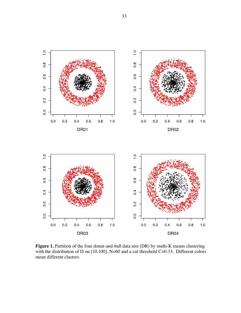
Three idealized, synthetic data sets with 2 or 3 designed clusters of different shapes were
generated (Figure 1-3). The synthetic data sets were designed to defeat typical clustering
algorithms except one in Figure 2 which was used as a control. Each data set contains 2000
points inside the unit square in R2 with 2 or 3 natural clusters. We refer to these as the donut-
and-ball (Figure 1, DR), horseshoe (Figure 2, U), and spiral (Figure 3, SP) data sets
respectively. For each of these three types we also designed four different examples of
varying difficulties (Ashlock, et al., 2005).
3.2 Clustering parameters
Euclidean distance is used to measure the distance between data points. There are 3
parameters that need to be defined for K-means multiclustering: the number of times to run
K-means clustering (N), the distribution of the number of clusters for each run (D) and the
cut off value for final clustering (C). Notice that C is in the range [0,1] due to the
normalization; the number of times two points are together is divided by the number of
clusterings performed to yield a connection strength that is always between 0 and 1 no matter
how many clusterings are performed. For all the 3 sets of synthetic data, K means clustering

14
is run for 60 times, each time the number of clusters K is chosen to be the uniform
distribution on [10,100], and the final clusters are determined by putting two data point in a
cluster if they have been clustered for more than 20 times, that is the cutoff value of 0.33.
3.3 Results
As shown in Figure 1-3, K-means multiclustering algorithm successfully discovers the
designed cluster structure of all the synthetic data, which is very hard for the traditional
clustering algorithms. Different color means different clusters. This demonstrates that the
algorithm can perform well on relatively idealized data that nevertheless are not well suited
to direct partition using traditional clustering algorithm via Euclidian metric. As we know
different distance metric prefers different shape of data, for example, Euclidian metric would
be better for data with round shape and correlation coefficient for elongated data set. The
designed data sets with different shapes, which are not preferred by Euclidian metric, can still
be correctly clustered by K-means multiclustering with Euclidian metric. It indicates that the
algorithm has a high level of immunity to artifacts introduced by the metric used to measure
the distance between data points. This immunity is obtained by amalgamating the results of
many k-means clusterings in a manner that builds the clusters from local information; most
metric artifacts has their origin in point pairs in the same cluster that are not close to one
another.

15
4 PROPERTIES AND PARAMETERS OF K-MEANS MULTICLUSTERING
4.1 Selection of the range of D and the number of times to cluster
The range of the distribution D and the number of clustering to perform vary with the
structure of the data. In order to study how the selection of D and N affects the performance
of K-means multiclustering algorithm, the multiclustering method was run with parameter
sets consisting of different values of D and N on synthetic data sets with two clusters (the
donut-and-ball data sets and the horseshoe data sets), three clusters (the spiral data set) and
eighty-one clusters (the G81 data set, Figure 4). The donut-and-ball, horseshoe and spiral
data sets are described in section 3.1. The G81 data set also contain 2000 data points inside
the unit square and has 81 designed disk-shaped clusters arranged in a nine-by-nine grid.
The need for the distribution D is worth at least a brief discussion. If the number of clusters
requested from the K-means algorithm is the same each time then the algorithm tends to find
the same clusters more often, based on noise features of the data, which can generate
artificial results. For the data used in this study, leaving the number of clusters computed the
same across a K-means multiclustering resulted in spuriously high connection strengths
between pairs of points near these repeating clusters. Changing the number of clusters
requested from the K-means algorithm through a broad rang of values eliminated this effect.
The distributions of D for idealized synthetic data sets with 2 or 3 clusters used 3 different
lower bound values for D (10, 60, 100) and 4 ranges with width (10, 40, 90, 190), while the
number of clusterings N was set to 5 different values (30, 60, 100, 200, 300). For the

16
idealized synthetic data set with 81 clusters, the lower bounds of Ds were set at 10, 100 and
300, three ranges 100, 200, and 300 were used, and five values for N were tested: 50, 100,
200, 400, 500. The range of cut-off values at which the right number of clusters was
detected, termed the correct cut off region, were calculated by running multiclustering
algorithm on the synthetic data sets using the various sets of parameters given. The larger
the correct cut off region is, the better the parameters selected is considered.
For the donut and ball (DR, Table 1), horse shoe (U, Table 2) and spiral (SP, Table 3) data
sets with 2 or 3 designed clusters, the more difficult the clustering problem posed by the data,
the narrower the correct cut off region. The SP data sets are more difficult than DR and U
data sets, the correct cut off regions of SP are narrower than those of DR and U. The range
of D with lower bound of 10 and medium widths [10, 50] and [10, 100] gave a larger correct
cut off region in most of the tests. The narrow range that was obtained with lower bound of
10, such as [10, 20], will either perform the best for easy data (e.g. DR01, U01, U03) sets or
the worst for hard data (e.g.: DR02, DR04, all SP). The wide range for the distribution D
with lower bound of 10, [10, 200] always gave smaller correct cut off regions that the
medium wide range with the same lower bound. Actually this is true for D with the higher
lower bound of 60 and 100. In general, for data sets with 2 or 3 clusters, the range of D with
lower bound of 10 and medium wideness are acceptable but the higher the lower bound, the
wider the range, the worse the correct cut off region. For harder data, wider ranges yield
better results than narrow ranges, but ranges that are too narrow or too wide perform poorly.
The medium width of D tested in this study functions adequately. For some of the harder
data sets (e.g. SP), a range for D with lower bound of 60 at narrow wideness yielding a range

17
of [60, 70] generates a better correct cut off region. If the range of D is fixed, varying the
number N of times to cluster does not change the size of the correct cut off region
dramatically, but for a wide range and high lower bound, larger N yield better results than
can be generated by any narrow range of D. Therefore, the selection of appropriate D is more
critical than the number of times the data are clustered. Considering the starting value of the
correct cut off region, the higher the lower bound and the wider the range of D, the lower the
start value becomes.
For the G81 data sets with 81 designed clusters (Table 3), the range of D of [10, 200] gave a
better correct cut off region for all 4 data sets, even for the hardest one G81D04. When D is
set to [100, 200] we obtain the best correct cut off region for G81D01. Choosing D with high
lower bound and wide range always gave the worst size of correct cut off region. It is a
surprise that the lower bound of D need not be larger than the real number of clusters. This is
probably because a larger lower bound and wider range would yield a graph with a large
number of moderate connection strengths that would not cut well. The cluster structure
would include a large number of small, spurious clusters.
4.2 The cut plot
The cut plot is an important feature of K-means multiclustering, which displays the number
of clusters across all possible cut weights. Once the algorithm has computed the connection
weights for all pairs of points it then computes the number of clusters that would results for
each value of C. Figure 5 shows the cut plot for donut-and-ball synthetic data set using

18
parameters defined in section 3.2 with D [10,100] and N = 60. The designed number of
clusters for this data set is two. Notice that all four cut plots have broad, flat regions which
give many values of C for which the number of cluster is two. The easiest data in Figure 1
DR01 gives two clusters at a cut value of zero which means that points in the donut and the
ball were never grouped together. The hardest data set in Figure 1 DR04 has the narrowest
region where the number of cluster is two, and the only one with a nontrivial flat region
where the number of clusters is more than two. The similar results of cut plot are also
obtained for horseshoe (Figure 6) and spiral (Figure 7) data sets. The results from our
synthetic data indicate that the cut plot gives guidance as to estimating strength of different
number of clusters, in the form of the broadness of the area of the cut plot that yields a give
number of clusters. A large flat area on the cut plot is a strong signal indicating the strength
of an estimate that the data contains a certain number of clusters, in essence it indicates that
the gap between clusters is much larger than the distance among nearest neighbors within
those clusters. The gap between clusters indicated by a flat region at the low cut off value in
a cut plot is larger than that between clusters with flat region at high cut off value. Examples
of data sets that has large distinguishable gap between clusters are the synthetic data sets
shown in Figure 1-3. When data has this character, the cut plot can give advice as to the
correct number of clusters. The cut plot also yields the information that there is no obvious
natural clusters if this is the case, that is there will be no significant flat area on the cut plot.
Therefore, the cut plot is a way to visualize the hierarchical structure of a data set.
A simple data set was generated to show how the cut plot can indicate the hierarchical data
structure. The data set has 25 data points with designed structure as shown in Figure 8. The
cut plot generated by K-means multiclustering algorithm with D [2, 7] and N 100 is shown in

19
Figure 8. This simple data set is designed to have 1, 2, 3 or 4 clusters depending on the
definition of clusters. The cut plot generated by K-means multiclustering can indicates this
kind of structure by showing the flat regions at 1, 2, 3, and 4 clusters. The gap between red
and blue clusters are more clear that that between the black and green clusters, which can be
reflected in the cut plot as a large flat region at 3 clusters.
Different runs of multiclustering algorithm can produce different cut plots, especially at high
cut off value, but the overall shape of the cut off plot remains the same. The variation of the
cut plot at high cut off value indicates the random factor effect on the clustering results; on
the other hand, the consistent part indicates the real data structure which can not be affected
by the random factor. Also different selections of multiclustering parameters can generate
different cut plots for a given data set, never the less the significant structure in the data stays
the same. The sort of simple summary of aspects of the structure of the data given by the cut
plot is potentially useful.
4.3 Hierarchical structure produced by K-means Multiclustering
In addition to the cut plot which can provide a simple summary of the data structure by, K-
means multiclustering can also provide a detailed view of the clusters formed to reveal the
underlying structure of the data with a hierarchical tree. The hierarchical tree built from
multiclustering algorithm shows how the data are merged into a cluster at different cut off
values, which is also an indicator of the hierarchical structure of the clusters of data points.

20
The data structure used to build the tree is shown in Figure 9. All the internal nodes are
linked by cluster_links (blue) to a specific cut off box. Those internal nodes are clusters at
specific cut off value. All the leaf nodes in a subtree of an internal node are all the data
points that belong to that cluster (internal node). Therefore, by traversing the subtree of an
internal node down to the leaves, we can find all the members of that cluster. A bottom-up
approach will be used to construct the tree where the end leaf nodes are individual data
points. The tree is initialized at a cut off of 100%, placing the data point in a cluster that
were invariably together. Data points in a cluster at a cut off 100% are linked by
sibling_link (green), and an internal cluster node will be generated, which is linked to cut off
array box at cut off 100%. The first data point node is linked to its cluster node by a
childred_link (red), and the rest of the data point leaf nodes are linked to their cluster node by
parent_links (black). As the cut off decreases, the existing internal nodes (clusters) at
previous cut off level would merge to form new internal nodes with larger number of leaf
nodes under them (more data elements in a cluster).
This cluster formation is basically the reflection of the connection strength between the data
points or the lower level clusters. K-means multiclustering algorithm can generate the tree in
text format which can be used to draw a tree with standard tree drawing software. A graphic
view of the resulting hierarchical tree can be presented as a dendrogram by tree drawing
software like Rainbow (http://genome.cs.iastate.edu/Rainbow/manual/). Figure 10 shows the
detailed tree view drawn by Rainbow of the hierarchical data structure of data set described
in section 4.2 (Figure 8).

21
5 RUNING K-MEANS MULTICLUSTERING ON SYNTHETIC MICROARRAY
DATA SETS
5.1 Synthetic microarry time series data sets
Because of a lack of unambiguous clusters for real biological microarry data set, it is difficult
to evaluate the performance of clustering methods on biological microarray data. A
collection of sixty simplified microarray time series data sets with six time points are
generated for this study. The sixty data sets are divided into 6 groups, each group consists of
10 data sets with the same number of designed clusters. The number of clusters in this study
are 5, 10, 15, 20, 25, 30. For each data set, the number of members in each cluster is picked
randomly from [10, 200]. Therefore, the data sets contain 500, 1,000, 1,500. 2,000, 2,500,
3000 data points for the 6 groups respectively. The pattern of fold change along 6 time
points of each cluster in a data set is expressed by a string like “012210”, which means
“down–no change-up-up-no change-down”. Strings designating the patterns are also selected
randomly, and the variance in fold change within each cluster is also randomly picked from
[0.05, 0.2]. These data sets are intended to simulate the microarray data which, after
statistical preprocessing including nomalization, standardization and significance testing,
have an idealized form. After preproccessing of biological data, clustering methods are run
on the genes already known to have statistically significant gene expression activity. For this
reason, no noise data (statistically non-significant data points) are simulated.

22
5.2 Clustering methods
In order to evaluate the relative performance of K-means multiclustering, three typical
clustering methods, Model-based clustering, hierarchical clustering and standard K-means
clustering, are used to cluster the 60 synthetic microarray data sets. Model-based clustering
was selected because the way we generate our synthetic data set fits the assumption of
model-based clustering method, which is that the data set is a finite Gaussian mixture, and
each cluster is represented by a Gaussian probability distribution. Therefore, Model-based
clustering can serve as a positive control. The hierarchical clustering method was selected
because K-means multiclustering can find the hierarchical structure of data sets. Comparing
the accuracy of the hierarchical structure generated by our method to the traditional
hierarchical clustering method is desirable. The model-based clustering we used in this study
is from the “Mclust” function implemented in an add-on R package “mclust”, and
hierarchical clustering and K-means clustering are from functions “hclust” and “kmean” in R
library “stats”.
5.3 Adjusted Rand Index
The Rand index (Rand, 1971) is a method to calculate the number of pair-wise agreement
and disagreement in two clustering results. Given two partitions into sets U and V, for all
possible pairs of data points i and j, there are four outcomes: a pair is together in both
partitions, in only the first, in only the second, or in neither. Let a be the number of pairs that
i and j are in same cluster in U and V; b is the number of pairs that i and j are in same cluster
in U, but not in V; c is number of pairs that i and j are in same cluster in V, but not in U; d is

23
the number of pairs that i and j are not in a cluster in both U and V. Hence, a and d describe
the agreement, b and c describe the disagreement. The Rand Index is then defined as:
!
R(U,V ) =(a + d)
(a + b + c + d)
The adjusted Rand Index (Hubert and Arabie, 1985; Yeung, et al., 2001) is calculated base
on the contingency table defined by U and V, where the value nij represents the number of
objects that are in the i th cluster in U and j th cluster in V. The adjusted Rand Index is given
as:
!
nij
2
"
# $
%
& ' (
ni.
2
"
# $
%
& '
n. j
2
"
# $
%
& '
j
)i
)*
+ , ,
-
. / / /n
2
"
# $ %
& '
ij
)
1
2
ni.
2
"
# $
%
& ' +
n. j
2
"
# $
%
& '
j
)i
)*
+ , ,
-
. / / (
ni.
2
"
# $
%
& '
n. j
2
"
# $
%
& '
j
)i
)*
+ , ,
-
. / / /n
2
"
# $ %
& '
The maximum values of the adjusted Rand Index is 1 when two partitions are the same. Its
expected value in the case of random clustering is 0. And the higher the adjusted Rand
Index, the higher the agreement between two partitions. Since the adjusted Rand Index is
more sensitive than Rand Index, we use adjusted Rand Index to compare the clustering
results from four clustering methods to the designed truth.
5.4 Comparison methods
There are two ways to compare different clustering results to the designed truth. The first
way is to pick a clustering result that gives the correct number of clusters. For our clustering
methods, we select the clustering results that give exactly the correct number of clusters or
the one that gives the number of clusters very close to the correct number if there is no

24
clustering result with the correct number of clusters. For the model-based and K-means
clustering methods, we give the correct number of clusters to the methods; for hierarchical
clustering we cut the tree at a joining strength chosen so as to generate clustering results with
the correct number of clusters.
The second comparison method is to find the clustering results that are closest to the truth,
which is in our case the clustering results that give the largest adjusted Rand Index. This
method will give us an idea about the ability of a method to reveal the designed data structure
under ideal circumstances. To find the clustering results with the best predicted data
structure revealed by our multiclustering algorithm, we calculate the adjusted Rand Index for
all clusterings with different number of clusters along the cut plot. For Model-based
clustering we give a wider range of number of clusters to the function; a wide range of
different cut value and number of clusters are fed to hierarchical clustering and K-means
methods respectively.
5.5 Consistency analysis
The multiclustering method is stochastic, and so different runs of the algorithm may generate
different clustering results. In order to study the performance consistency of K-means
multiclustering methods, five runs of K-means multiclustering are conducted on all 60
synthetic microarry time series data sets. The distribution of D in this study is uniform on
[10,100] and run 500 times.

25
From Figure 12, we can see that the 5 different runs have the very similar best adjusted Rand
Index (the second comparison method) on the 60 synthetic microarry data sets. The standard
deviations for the adjusted Rand Indices of 5 runs on all the synthetic data sets tested are all
less than 0.02; the average best adjusted Rand Indices are above 0.95 (Table 6). The
consistently high vale of the best Rand Indices for all data sets indicate that multiclustering
method is reliable in finding the designed clusters.
The adjusted Rand Indices of the five runs based on the clustering results with the best guess
as to the number of cluster, i.e. the first comparison method, fluctuate more than those with
the best Rand Index (Figure 11). Of the 60 data sets, the five runs on eleven of them have
standard deviations of above 0.03 (Table 5). The group of synthetic data sets with 30 clusters
has the lowest average adjusted Rand Index of 0.86, and the rest sets with less than 30
clusters have the average adjusted Rand Index above 0.93.
The more the clusters in a data set, the smaller the gap between clusters. This, in turn, means
that the data set is more difficult to cluster correctly at cut values that yield more clusters. A
consistent result from the two different comparison methods is that muticlustering has better
performance (i.e. higher adjusted RandIndex value) on data sets with fewer clusters than
those with more clusters. For almost all data sets except one in groups with 5 clusters,
multiclustering algorithm can find the perfect clustering results. Comparing with the
adjusted Rand Indices of the second comparison method, the adjusted RandIndices of the
first comparison method are not as stable. The data sets with fluctuating adjusted Rand
Indices from different runs are not only in groups with more clusters. Almost all groups

26
except the group with 10 clusters have data sets with fluctuating adjusted Rand Index. This
suggests that the number of clusters is not the major reason for instability of the
multiclustering results. We guess the reason might be the big variation within the clusters or
very similar the fold change patterns among clusters. For those data sets that exhibit slightly
different results in different runs, the variation may also reflect the random factors in the
operation of the clustering algorithm. The variation between runs may thus be useful for
determining which clusters the data actually support. The results from the two methods are
very close for data set with fewer clusters, which indicates that multiclutering algorithm can
find both the right number of clusters and right structure for data sets with fewer clusters, but
not the right number of clusters for data sets with more clusters. The stable best adjusted
RandIndex and fluctuated Rand Index of the first method among 5 runs suggest that the most
accurate clustering results generated by K-means multiclustering are very stable, even though
the number of clusters may change, or stray from the designed structure. This shows the
consistency in the ability to identify the designed data structure.
5.6 The effect of parameter settings
Based on our experience from our synthetic data set, that is the distribution of D [10,100]
works fine when the number of clusters is less than 100, three distributions for D are used:
uniform on each of [10,100], [10, 50], and [50, 100].
Using the first comparison method, we can see that different Ds seem have less impact on
performance for the synthetic data sets with the numbers of clusters less than 20 (Figure 13).

27
The most different adjusted RandIndices (first method) from different Ds can be found in the
data sets with 30 clusters. For data sets with over 20 clusters, there is no a single distribution
of D that would get the best performance for all the data sets. This may be because for data
sets with fewer numbers of clusters the complexity of the data sets is less, therefore for hard
data set, to get the right number of clusters and right structure the selection of D is very
important.
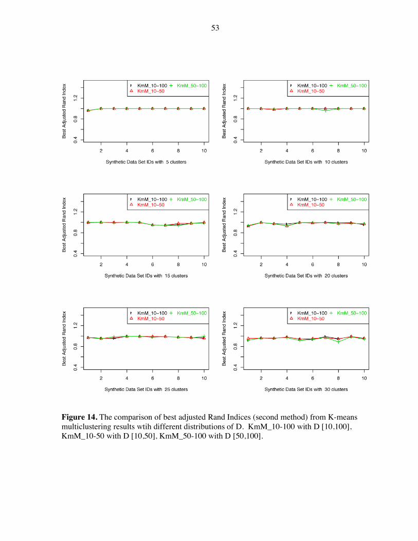
When we use the second comparison method, different distributions of D give very similar
best adjusted Rand Index values (Figure 14) for all the data sets with different number of
clusters; in this case the selection of parameters does not affect the ability of the algorithm to
find the designed data structure.
5.7 Performance comparison among clustering methods
The average of adjusted Rand Indices from the five runs of K-means multiclustering (as
described in section 5.5) is used as the clustering result of multiclustering algorithm for the
performance comparison to the other three clustering methods.
For the first comparison method (Figure 15, Table 7), multiclustering finds the perfect
clustering results with adjusted Rand Indices of 1.0 for 9 data sets out of 10 with 5 clusters;
Model-based clustering performs poorly on 3 out those 10 data sets. For the forty data sets
with 10 – 25 clusters, K-means multiclustering has the similar adjusted RandIndices as
Model-based clustering methods except 3 data sets. Model-based clustering method shows

28
the best performance for the 10 data sets with 30 clusters; in general multiclustering is the
second best. The performance of hierarchical clustering and K-means clustering varies
greatly from data sets to data sets, while multiclustering has up and down in the adjusted
RandIndices only in data sets with 30 clusters. Except one data set with 15 clusters,
multiclustering method shows superior or similar clustering compared to hierarchial
clustering method. As we expected, multiclusering performs better than K-means clutering,
but it is interesting to find that K-means is slightly better than multiclustering on two data
sets with 30 clusters. We use the same distribution of D on all the data sets for this study, as
we mentioned before there is no universal parameters that fit to all data sets, different
distribution of D may help to find the right number of clusters and right structure at the same
time. In general, when we consider the ability of clustering methods to find the right number
and right structure of clusters, multiclustering method is similar to the positive control
method, i.e. Model-based clustering, on data sets with fewer clusters and better than the two
other traditional clustering methods – hierarchical clustering and K-means clustering.
In comparison to other methods, the results from the second comparison method (Figure 16,
Table 8) show that for almost all the 60 data sets, multiclustering is the method with the
highest best adjusted Rand Index, which means that it can find the clustering closest to the
truth. The best adjusted Rand Indices of the multiclustering algorithm for all data sets are
above 0.9. For some data sets multiclustering has higher best adjusted Rand Indices than the
positive control method – Model-based clustering. Not like the adjusted Rand Indices
computed by the first method, the best adjusted Rand Indices of multiclustering do not vary
from data sets to data sets, which show the ability of multiclusetering to consistently find the

29
right data structure for different data sets with high accuracy. Combining the results from
section 5.5 and 5.6, we can see that the ability of multiclustering algorithm to discover the
real data structure, which is measured by the adjusted Rand Index by the second comparison
method, is stable from different runs, different distribution of D, and different data sets. This
indicates the strong ability of multiclustering to capture the natural shape of data sets.
The ultimate goal of clustering is to explore the data set and divided the data points into
groups based on their relationship. In most cases, the nature dividing of the data is not clear,
the number of clusters is really depending on the definition of clusters. The internal
relationship among data points, which is helpful to interpret the underlying meaning carried
by the data, is the most important thing for scientist. Therefore, a good clustering method
should be able to reveal the underlying data structure. As we show above multiclustering has
the ability of capturing the designed data structure of synthetic microarray data sets with high
accuracy, it would be a useful tool for biologist to explore microarray data.
6 DISCUSSION AND CONCLUSIONS
This manuscript introduces, defines, and tests multiclustering. It is found to be reliable and
consist in capturing the underlying data structure, and competitive with model based
clustering and superior to other methods on data generated in a manner consistent with the
hypothesis of model based clustering. Data which are poorly conditioned relative to the
assumptions of model based clustering may be a domain where the ability of multiclustering
to function without a model will yield clearly superior performance. The ability of
multiclustering to reduce artifacts due to the choice of metric used to compare data points

30
and to function without a model for the distribution of the data reduce the number of
assumptions that must be made. This study demonstrates that multiclustering is relatively
robust to the parameter choices to find the right number of clusters and the right structure that
must be made and gives some rules of thumb for choosing those parameters. The selection
of the distribution of D is more critical than that of N, the number of cluterings to perform.
High lower bounds (too far away from the real number of clusters) and wide ranges for D are
not favored by our testing data sets with 2, 3 and 81 clusters. For the same type of data,
wider ranges for D would be helpful to data sets with smaller gaps between clusters.
A difficulty in interpreting microarry clustering results is the fact that, given a data set, a
clustering method can always generate clusters for it. In some cases different clustering
methods will produce very different clusters. People may misinterpret the data by examining
improperly clustered data; the use of clustering thus puts a larger burden on the researcher to
make careful interpretations. The distance or similarity metric chosen, the computational
preparation of the data prior to clustering, and the choice of which data to disregard are all
possible sources of algorithmic artifacts in clustering. Careful examination is required to
check if the clusters are natural clusters instead of artifacts of the algorithm. Another
difficulty in clustering microarray data is that there is no clear definition of cluster. The
clustering results are often based on the relative distance among data points. A single
clustering result will not reflect the overall relationship among the data points. Therefore, the
hierarchical tree generated by multiclustering is a better way to show the underlying data
structure. Instead of giving a clustering result, the multiclustering algorithm produces a
hierarchical tree which gives the whole picture of the relative relationship among data points.

31
This provides biologists a more complete view of the whole data set, which would help them
to discover and interpret the underlying biological meaning. Therefore, the multiclustering
algorithm that can consistently identify the data structure with high accuracy that is
comparable to that of model-based clustering on data sets that are designed to follow the
assumption of Model-based clustering, and display the over all data structure using a
hierarchical tree is helpful tool for biology to explore the relationship among genes in which
they are interested.
In spite of the shortcomings of clustering, it is still a powerful tool for microarray analysis.
Since the scale of information generated by a microarray experiment is far beyond the level
that can be handled by human without some form of computational assistance. The major
purpose of clustering in microarray analysis is to reduce the data to the level that biologist
can generate hypothesis, or explain the relations between genes and phenotypes. Therefore,
the relationships between clusters of genes and phenotypes predicted on clustering based
analysis are tentative. Keeping this in mind and along with the intensive research effort to
more accurate clustering method, we can avoid, or at least minimize misunderstandings.
Finally, the accuracy of the clustering methods also depends on the quality of the microarray
data and the statistical approach used to preprocess the raw data.
ACKNOWLEDGEMENTS
We thank Duhong Chen for providing “RainBow” tree drawing software. This project was
supported by competitive grants from the National Science Foundation Plant Genome
Program (DBI-9975868 and DBI-0321711).

32
REFERENCES
Ashlock, D., Kim, E.Y. and Guo, L. (2005) Multi-clustering: Avoiding The Natural Shape of Underlying Metrics, ANNIE 2005. D'Haeseleer, P. (2005) How does gene expression clustering work?, Nat Biotechnol, 23, 1499-1501. DeRisi, J.L., Iyer, V.R. and Brown, P.O. (1997) Exploring the metabolic and genetic control of gene expression on a genomic scale, Science, 278, 680-686. Eisen, M.B., Spellman, P.T., Brown, P.O. and Botstein, D. (1998) Cluster analysis and display of genome-wide expression patterns, Proc Natl Acad Sci U S A, 95, 14863-14868. Ghosh, D. and Chinnaiyan, A.M. (2002) Mixture modelling of gene expression data from microarray experiments, Bioinformatics, 18, 275-286. Hubert, L. and Arabie, P. (1985) Comparing partitions Journal of Classification, 193-218. Jiang, D.T., C. Zhang, A. (2004) Cluster analysis for gene expression data: a survey, IEEE Transactions on knowledge and Data Engineering, 16, 1370-1386. McQueen, J.B. (1967) Some methods for classification and analysis of multivariate observations. , 1, 281-297. Rand, W. (1971) Objective criteria for the evaluation of clustering methods, Journal of the American Statistical Association, 66, 846-850. Swift, S., Tucker, A., Vinciotti, V., Martin, N., Orengo, C., Liu, X. and Kellam, P. (2004) Consensus clustering and functional interpretation of gene-expression data, Genome Biol, 5, R94. Wu, L.F., Hughes, T.R., Davierwala, A.P., Robinson, M.D., Stoughton, R. and Altschuler, S.J. (2002) Large-scale prediction of Saccharomyces cerevisiae gene function using overlapping transcriptional clusters, Nat Genet, 31, 255-265. Yeung, K.Y., Fraley, C., Murua, A., Raftery, A.E. and Ruzzo, W.L. (2001) Model-based clustering and data transformations for gene expression data, Bioinformatics, 17, 977-987.
33
Figure 1. Partition of the four donut-and-ball data sets (DR) by multi-K means clustering with the distribution of D on [10,100], N=60 and a cut threshold C=0.33. Different colors mean different clusters.

34
Figure 2. Partition of the four horseshoe data sets (U) by multi-K means clustering with the distribution of D on [10,100], N=60 and a cut threshold C=0.33. Note that the fourth data set can be correctly clustered with standard K-means clustering.

35
Figure 3. Partition of the four spiral data sets (SP) by K-means multiclustering with the distribution of D on [10,100], N=60 and a cut threshold C=0.33.

36
Figure 4. Partition of the four G81 data sets by K-means multiclustering with the distribution of D on [10,200], N=60 and a cut threshold C=0.56.

37
Table 1. The best and worst10 parameter settings for all four DR sets
The best The worst Parameters Cut off Parameters Cut off
Data sets
D1 N2 Start3 Width4 D1 N2 Start3 Width4 [10,20] 60 2 84 [100,290] 300 2 33 [10,20] 30 3 83 [100,140] 200 2 30 [10,20] 200 2 81 [100,140] 300 2 30 [10,20] 300 2 81 [100,190] 100 2 30 [10,20] 100 2 80 [100,140] 60 2 27 [10,50] 30 3 79 [100,190] 60 2 27 [10,50] 60 2 74 [100,140] 30 3 26 [10,50] 100 2 74 [100,190] 30 3 26 [10,50] 200 2 73 [100,290] 30 3 26
DR01
[10,50] 300 2 72 [100,140] 100 2 25 [10,50] 60 22 51 [100,290] 30 7 30 [10,50] 100 21 50 [100,290] 60 3 30 [10,100] 200 17 49 [100,110] 100 4 28 [10,50] 300 25 48 [100,110] 60 3 27 [10,100] 300 18 48 [100,110] 30 7 23 [10,50] 200 25 47 [10,20] 300 61 15 [10,100] 30 27 46 [10,20] 100 64 13 [10,100] 100 19 46 [10,20] 200 64 11 [60,70] 60 13 44 [10,20] 30 67 10
DR02
[10,50] 30 30 43 [10,20] 60 72 1 [10,50] 200 8 67 [100,110] 100 2 37 [10,50] 100 8 66 [100,190] 100 2 37 [10,50] 300 9 66 [100,290] 200 2 37 [10,50] 60 8 65 [100,190] 60 2 35 [10,50] 30 13 60 [100,290] 300 2 35 [10,20] 200 25 56 [100,110] 30 3 34 [10,20] 300 26 56 [100,290] 30 3 34 [10,100] 60 10 55 [100,190] 200 2 33 [10,100] 100 7 53 [100,190] 300 2 32
DR03
[10,100] 200 6 53 [100,290] 60 2 31 1 D is the distribution of the number of clusters for each run 2 N is the number of times to run K-means clustering 3 The lowest cut off value at which the correct number of clusters is found 4 The width correct cut off

38
Table 1. (continued) The best The worst
Parameters Cut off Parameters Cut off Data sets
D1 N2 Start3 Width4 D1 N2 Start3 Width4 DR04 [10,100] 300 22 41 [100,110] 60 12 20
[10,100] 200 23 39 [100,190] 200 10 20 [10,100] 100 26 36 [100,290] 30 17 20 [10,200] 300 14 36 [100,190] 30 23 17 [10,100] 60 27 35 [100,110] 30 20 13 [10,200] 60 18 35 [10,20] 30 70 7 [10,200] 200 16 35 [10,20] 60 75 2 [60,70] 300 21 35 [10,20] 100 72 2 [60,150] 200 11 35 [10,20] 300 72 2 [60,150] 300 10 35 [10,20] 200 72 1

39
Table 2. The best and worst10 parameter settings for all four U data sets
The best The worst Parameters Cut off Parameters Cut off
Data sets
D N Start Width D N Start Width [10,20] 60 10 70 [100,190] 30 3 34 [10,20] 100 10 68 [100,190] 200 2 34 [10,20] 200 12 68 [100,190] 300 2 34 [10,50] 60 3 67 [60,250] 60 2 30 [10,20] 30 17 66 [100,290] 100 2 27 [10,20] 300 11 66 [100,290] 300 2 27 [10,50] 300 3 64 [100,290] 200 2 26 [10,100] 60 3 64 [60,250] 30 3 20 [10,50] 30 7 63 [100,290] 30 3 20
U01
[10,50] 200 3 63 [100,290] 60 2 18 [10,50] 30 10 67 [60,250] 300 2 35 [10,100] 60 3 64 [100,190] 60 2 35 [10,100] 100 4 64 [60,250] 100 2 34 [10,50] 200 13 63 [60,250] 200 2 34 [10,50] 300 12 63 [60,250] 60 3 32 [10,100] 200 6 63 [100,290] 60 2 31 [10,100] 300 8 63 [100,290] 100 2 29 [10,50] 60 13 62 [100,290] 200 2 28 [10,50] 100 12 61 [100,290] 300 2 25
U02
[10,100] 30 7 60 [100,290] 30 3 24 [10,20] 60 13 72 [100,190] 60 2 36 [10,50] 100 3 72 [100,190] 100 2 36 [10,50] 300 4 72 [100,140] 60 2 35 [10,20] 200 13 71 [100,190] 200 2 35 [10,50] 200 4 71 [60,250] 100 2 34 [10,20] 300 13 70 [100,290] 60 2 31 [10,20] 100 12 69 [100,290] 30 3 27 [10,100] 60 5 68 [100,290] 300 2 27 [10,50] 60 3 67 [100,290] 200 2 26
U03
[10,100] 30 3 67 [100,290] 100 2 25 [10,50] 60 2 75 [60,250] 30 3 34 [10,50] 30 3 74 [100,140] 100 2 34 [10,50] 100 2 72 [100,190] 200 2 34 [10,50] 300 2 72 [100,190] 300 2 34 [10,50] 200 2 71 [100,290] 30 3 34 [10,20] 30 10 70 [100,140] 200 2 33 [10,20] 60 8 69 [100,290] 60 2 28 [10,20] 300 6 67 [100,290] 100 2 27 [10,100] 30 3 67 [100,290] 300 2 25
U04
[10,100] 300 2 67 [100,290] 200 2 24

40
Table 3. The best and worst10 parameter settings for all four SP data sets
The best The worst Parameters Cut off Parameters Cut off
Data sets
D N Start Width D N Start Width [10,50] 100 29 38 [60,250] 30 3 7 [10,50] 60 33 35 [100,290] 100 2 7 [10,50] 200 32 32 [100,290] 200 2 7 [10,50] 300 29 32 [60,250] 100 2 6 [60,70] 200 2 28 [100,290] 300 2 6 [10,50] 30 40 27 [10,20] 30 73 4 [60,70] 30 3 27 [10,20] 60 78 4 [60,70] 100 2 27 [10,20] 100 77 2 [60,70] 300 2 27 [10,20] 200 79 2
SP01
[60,100] 30 3 27 [10,20] 300 0 0 [60,70] 100 2 49 [60,250] 60 2 25 [10,50] 100 25 47 [100,290] 100 2 25 [60,70] 60 2 46 [60,250] 30 3 24 [10,50] 300 26 45 [60,250] 100 2 23 [60,100] 60 2 45 [100,290] 60 2 23 [10,50] 200 27 44 [10,20] 60 63 10 [10,100] 300 10 44 [10,20] 100 66 9 [60,70] 30 3 44 [10,20] 30 67 6 [60,70] 300 2 44 [10,20] 300 70 4
SP02
[60,100] 30 3 44 [10,20] 200 71 2 [60,70] 200 2 43 [100,290] 30 3 14 [60,70] 300 2 42 [100,290] 60 3 14 [10,100] 300 13 39 [60,250] 30 7 13 [60,100] 200 2 38 [100,290] 300 3 13 [10,100] 30 20 37 [10,50] 30 37 6 [10,100] 100 12 37 [10,20] 60 78 4 [10,100] 200 13 37 [10,20] 100 78 1 [60,70] 60 3 37 [10,20] 200 78 1 [60,100] 30 3 37 [10,20] 30 0 0
SP03
[60,70] 100 2 36 [10,20] 300 0 0 [10,50] 200 30 44 [100,140] 30 10 23 [10,100] 30 13 44 [100,290] 200 5 23 [60,70] 100 5 44 [60,250] 60 8 22 [60,70] 200 5 44 [100,290] 30 3 20 [10,50] 100 33 43 [100,290] 60 3 19 [10,50] 300 30 42 [10,20] 30 77 3 [10,100] 60 13 42 [10,20] 60 77 1 [10,100] 200 14 42 [10,20] 200 78 1 [10,100] 300 13 42 [10,20] 100 0 0
SP04
[10,100] 100 13 40 [10,20] 300 0 0

41
Table 4. The best and worst10 parameter settings for all four G81 data sets
The best 10 The worst Parameters Cut off Parameters Cut off
Data sets
D N Start Width D N Start Width [100,200] 100 37 27 [300,500] 500 2 6 [10,200] 50 56 22 [300,400] 50 2 6 [100,200] 200 42 19 [10,100] 100 84 6 [100,400] 50 12 18 [300,600] 400 2 5 [100,300] 50 18 18 [300,600] 50 2 4 [100,200] 50 38 18 [300,600] 200 2 4 [100,400] 100 14 16 [300,600] 500 2 4 [10,200] 100 62 16 [300,500] 50 2 4 [100,300] 200 26 15 [300,500] 200 2 4
G81D01
[100,400] 400 18 14 [300,600] 100 2 3 [10,200] 50 46 30 [100,200] 50 32 8 [10,100] 100 63 24 [300,400] 400 3 8 [10,100] 200 67 23 [300,500] 50 2 8 [10,100] 50 66 22 [300,500] 100 2 7 [10,300] 100 36 22 [300,500] 200 2 7 [100,300] 50 18 22 [300,600] 100 2 6 [100,400] 50 12 22 [300,600] 200 2 6 [10,200] 100 56 20 [300,600] 400 2 6 [10,300] 50 32 20 [300,600] 500 2 5
G81D02
[10,100] 400 72 18 [300,600] 50 4 4 [10,200] 50 46 28 [300,500] 500 5 2 [100,300] 50 18 28 [300,600] 100 3 2 [10,300] 100 37 26 [300,600] 400 4 2 [10,100] 200 60 24 [300,600] 500 4 2 [100,200] 50 30 24 [300,500] 100 4 1 [100,400] 50 12 24 [300,500] 200 6 1 [10,200] 100 52 22 [300,600] 200 4 1 [10,300] 50 36 22 [300,400] 100 0 0 [100,400] 100 13 22 [300,500] 50 0 0
G81D03
[10,100] 400 64 21 [300,600] 50 0 0 [10,200] 400 46 20 [100,300] 400 0 0 [10,100] 400 59 19 [100,300] 500 0 0 [10,200] 200 46 19 [300,400] 100 0 0 [10,200] 500 46 19 [300,400] 400 0 0 [10,100] 500 61 17 [300,400] 500 0 0 [10,100] 200 65 13 [300,500] 50 0 0 [100,200] 200 38 13 [300,500] 200 0 0 [100,200] 500 39 13 [300,500] 500 0 0 [10,200] 100 51 12 [300,600] 50 0 0
G81D04
[10,300] 50 40 12 [300,600] 400 0 0

42
Figure 5. The cut plots for the four dount-and-ball data sets (DR) produced by the K-means multiclustering method with the distribution of D [10,100] and N=60.

43
Figure 6. The cut plots for the four horseshoe data sets (U) produced by the K-means multiclustering method with the distribution of D [10,100] and N=60.

44
Figure 7. The cut plots for the four spiral data sets (SP) produced by the K-means multiclustering method with the distribution of D [10,100] and N=60.

45
Figure 8. The data set with 25 data points and designed structure of 2, 3, and 4 clusters (upper panel) and its cut plot computed by K-means multiclustering with D [2,7], N=100.

46
Figure 9. Detailed data structure for building hierarchical tree of clusters generated by K-means multiclustering means algorithm

47
Figure 10. The detailed hierarchical tree view of the synthetic data set with 25 data points in Figure 8.

48
Figure 11. The adjusted Rand Indices (first comparison method) of 5 runs of K-means multiclustering with D [10,100], N=500 on 60 synthetic microarray data sets

49
Table 5. The average and standard deviation of adjusted Rand Indices (first method) from 5 runs of K-means multiclustering (D [10,100], N=500) on 60 synthetic microarray data sets
No. of clusters in data sets Data sets ID 5 10 15 20 25 30
1 0.947±0.066 1.000±0.000 0.994±0.000 0.858±0.011 0.835±0.045 0.873±0.000 2 1.000±0.000 0.998±0.000 1.000±0.000 0.977±0.003 0.933±0.032 0.863±0.000 3 1.000±0.000 0.954±0.000 0.997±0.000 0.916±0.042 0.892±0.000 0.734±0.071 4 1.000±0.000 1.000±0.000 0.999±0.000 0.934±0.018 0.993±0.001 0.944±0.015 5 1.000±0.000 1.000±0.000 0.993±0.003 0.975±0.036 0.989±0.002 0.902±0.002 6 1.000±0.000 1.000±0.000 0.862±0.000 0.986±0.000 0.960±0.007 0.718±0.003 7 1.000±0.000 0.997±0.000 0.925±0.041 0.920±0.037 0.989±0.002 0.923±0.019 8 1.000±0.000 1.000±0.000 0.888±0.051 0.902±0.049 0.978±0.000 0.825±0.027 9 1.000±0.000 1.000±0.000 0.979±0.000 0.924±0.014 0.952±0.008 0.969±0.023
10 1.000±0.000 1.000±0.000 0.998±0.000 0.946±0.010 0.951±0.000 0.933±0.000

50
Figure 12. The best adjusted Rand Indices (second comparison method) of 5 runs of K-means multiclustering with D [10,100] N=500 on 60 synthetic micoarray data sets

51
Table 6. The average and standard deviation of best adjusted Rand Indices (second method) from 5 runs of K-means multiclustering (D [10,100], N=500) on 60 synthetic microarray data sets
No. of clusters in data sets Data sets ID 5 10 15 20 25 30
1 0.982±0.019 1.000±0.000 0.996±0.003 0.930±0.010 0.971±0.003 0.925±0.014 2 1.000±0.000 0.998±0.000 1.000±0.000 0.996±0.000 0.952±0.007 0.969±0.010 3 1.000±0.000 0.981±0.000 0.997±0.000 0.979±0.006 0.961±0.010 0.965±0.007 4 1.000±0.000 1.000±0.000 0.999±0.000 0.962±0.009 0.995±0.001 0.980±0.001 5 1.000±0.000 1.000±0.000 0.996±0.002 0.994±0.000 0.994±0.000 0.941±0.006 6 1.000±0.000 1.000±0.000 0.941±0.010 0.989±0.004 0.989±0.006 0.946±0.010 7 1.000±0.000 0.997±0.000 0.939±0.011 0.998±0.002 0.990±0.000 0.975±0.011 8 1.000±0.000 1.000±0.000 0.971±0.013 0.978±0.011 0.978±0.000 0.932±0.011 9 1.000±0.000 1.000±0.000 0.980±0.001 0.988±0.007 0.974±0.011 0.987±0.005
10 1.000±0.000 1.000±0.000 0.996±0.004 0.960±0.010 0.970±0.011 0.962±0.007

52
Figure 13. The comparison of adjusted Rand Indices (first method) from K-means multiclustering results with different distribution of D. KmM_10-100 with D [10,100], KmM_10-50 with D [10,50], KmM_50-100 with D [50,100].
53
Figure 14. The comparison of best adjusted Rand Indices (second method) from K-means multiclustering results wtih different distributions of D. KmM_10-100 with D [10,100], KmM_10-50 with D [10,50], KmM_50-100 with D [50,100].

54
Figure 15. The comparison of performance (first method) of four clustering algorithms. KmM: K-means Multiclustering, MC: Mode-based Clustering, HC: Hierarchical Clustering, Km: K-means Clustering

55
Table 7. The adjusted Rand Indices (first method) of 60 microarray synthetic data sets from four clustering algorithm
Data sets No. of clusters
Data sets IDs
K-means multiclustering
Model-based
clustering
Hierarchical clustering
K-means clustering
1 0.947 1 0.93 0.933 2 1 1 1 0.979 3 1 1 0.916 0.988 4 1 0.865 0.897 0.802 5 1 1 1 0.948 6 1 1 0.854 0.997 7 1 1 1 1 8 1 0.696 0.943 0.933 9 1 0.599 0.964 0.608
5
10 1 1 0.997 0.957 1 1 0.943 0.868 0.731 2 0.998 0.937 0.812 0.886 3 0.954 1 0.963 0.943 4 1 1 0.949 0.989 5 1 1 0.857 0.949 6 1 1 0.831 0.905 7 0.997 1 0.844 0.839 8 1 1 0.946 0.877 9 1 1 0.986 0.984
10
10 1 1 0.937 0.931 1 0.994 1 0.922 0.908 2 1 1 0.814 0.803 3 0.997 0.999 0.929 0.85 4 0.999 0.964 0.913 0.937 5 0.993 0.964 0.901 0.944 6 0.862 0.951 0.944 0.845 7 0.925 0.969 0.903 0.982 8 0.888 0.943 0.846 0.804 9 0.979 0.996 0.943 0.893
15
10 0.998 0.968 0.884 0.874 1 0.858 1 0.922 0.842 2 0.977 0.988 0.825 0.746 3 0.916 0.953 0.766 0.704 4 0.934 0.935 0.874 0.859 5 0.975 0.926 0.856 0.82
20
6 0.986 0.979 0.706 0.895

56
Table 7. (continued) Data sets
No. of clusters
Data sets IDs
K-means multiclustering
Model-based
clustering
Hierarchical clustering
K-means clustering
7 0.92 0.917 0.921 0.827 8 0.902 0.903 0.814 0.874 9 0.924 0.991 0.886 0.914
10 0.946 0.961 0.816 0.815 1 0.835 0.957 0.882 0.838 2 0.933 0.962 0.864 0.823 3 0.892 0.96 0.805 0.851 4 0.993 0.95 0.993 0.825 5 0.989 0.971 0.879 0.812 6 0.96 0.963 0.901 0.893 7 0.989 0.978 0.954 0.876 8 0.978 0.933 0.852 0.856 9 0.952 0.963 0.946 0.876
25
10 0.951 0.95 0.922 0.819 1 0.873 0.984 0.886 0.785 2 0.863 0.969 0.801 0.852 3 0.734 0.966 0.789 0.776 4 0.944 0.942 0.846 0.862 5 0.902 0.973 0.909 0.809 6 0.718 0.968 0.754 0.781 7 0.923 0.98 0.885 0.845 8 0.825 0.967 0.808 0.785 9 0.969 0.938 0.877 0.829
30
10 0.933 0.972 0.869 0.761

57
Figure 16. The comparison of performance (second method) of four clustering algorithms. KmM: K-means Multiclustering, MC: Mode-based Clustering, HC: Hierarchical Clustering, Km: K-means Clustering

58
Table 8. The best adjusted Rand Indices (second method) of 60 microarray synthetic data sets from four clustering algorithms
Data sets No. of clusters
Data sets IDs
K-means multiclustering
Model-based
clustering
Hierarchical clustering
K-means clustering
1 0.982 1 0.93 0.933 2 1 1 1 0.979 3 1 1 0.988 0.988 4 1 0.963 0.997 0.987 5 1 1 1 0.93 6 1 1 0.998 0.997 7 1 1 1 1 8 1 0.97 0.973 0.966 9 1 0.696 0.975 0.764
5
10 1 1 0.997 0.957 1 1 0.841 0.887 0.868 2 0.998 0.937 0.91 0.866 3 0.981 1 0.974 0.955 4 1 1 0.992 0.989 5 1 1 0.986 0.992 6 1 0.929 0.831 0.93 7 0.997 1 0.884 0.927 8 1 1 0.946 0.935 9 1 1 0.994 0.947
10
10 1 1 0.937 0.963 1 0.996 1 0.952 0.89 2 1 1 0.943 0.959 3 0.997 0.999 0.936 0.882 4 0.999 0.974 0.975 0.913 5 0.996 0.986 0.974 0.949 6 0.941 0.988 0.96 0.928 7 0.939 0.991 0.933 0.93 8 0.971 0.963 0.846 0.808 9 0.98 0.996 0.954 0.966
15
10 0.996 0.992 0.932 0.902 1 0.93 0.944 0.935 0.892 2 0.996 0.997 0.892 0.891 3 0.979 0.973 0.848 0.824 4 0.962 0.935 0.88 0.859 5 0.994 0.979 0.929 0.906
20
6 0.989 0.995 0.962 0.92

59
Table 8. (continued) Data sets
No. of clusters
Data sets IDs
K-means multiclustering
Model-based
clustering
Hierarchical clustering
K-means clustering
7 0.998 0.917 0.949 0.896 8 0.978 0.897 0.85 0.85 9 0.988 0.968 0.931 0.873
10 0.96 0.988 0.932 0.883 1 0.971 0.968 0.884 0.838 2 0.952 0.903 0.878 0.891 3 0.961 0.941 0.845 0.842 4 0.995 0.88 0.995 0.92 5 0.994 0.917 0.881 0.904 6 0.989 0.977 0.952 0.904 7 0.99 0.978 0.969 0.918 8 0.978 0.956 0.889 0.872 9 0.974 0.997 0.969 0.949
25
10 0.97 0.973 0.947 0.907 1 0.925 0.996 0.915 0.864 2 0.969 0.996 0.883 0.876 3 0.965 0.961 0.861 0.808 4 0.98 0.916 0.925 0.864 5 0.941 0.95 0.94 0.875 6 0.946 0.98 0.836 0.819 7 0.975 0.996 0.909 0.846 8 0.932 0.918 0.814 0.827
30
9 0.987 0.938 0.917 0.863

60
CHAPTER 3. A NEW INTEGRATED GENETIC AND PHYSICAL MAP OF MAIZE
REVEALS CHROMOSOME LEVEL ORGANIZATION OF GENE EXPRESSION
PATTERNS
Ling Guo, Hsin D. Chen, Kai Ying, Karthik Viswanathan, Tsui-Jung Wen, Olga Nikolova,
Natalja Zazubovits, Scott J. Emrich, Daniel A. Ashlock, Patrick S. Schnable
A manuscript to be submitted to Genetics
ABSTRACT
A high-density genetic map, ISU-IBM Map7, of maize was constructed by integrating
~3,300 existing markers and 4,700 new InDel Polymorphism (IDP) markers derived from
genes and predicted genes. Over 1,800 of these IDPs are codominant markers that can be
detected via Temperature Gradient Capillary Electrophoresis (TGCE). Because IDP markers
are sequence based, they can be used to integrate the genetic and physical maps using
sequence similarity rather than hybridization-based approaches. As of February 2007 the
maize physical map created by the Arizona Genome Institute (AGI) contained 292,502 BACs
grouped into 721 finger print contigs (FPCs) and singletons. As of 2/2/2007 ~6,430 of these
had been at least partially sequenced by the maize genome sequencing project. The
sequences of 418 FPCs match at least one marker from ISU-IBM Map7 and 322 FPCs match
at least two closely linked markers. Sixty-nine of these 322 FPCs had not previously been
anchored by hybridization-based approaches. Using this integrated genetic/physical map it
was possible to position 2,146 genes from the maize cDNA microarray SAM1.0 on the map.

61
Analysis of microarray data revealed statistically significant differences in the distribution of
strongly and weakly expressed genes across multiple chromosomes. This finding
demonstrates the existence of chromosome level regulation of gene expression. All project
data are available at: http://maize-mapping.plantgenomics.iastate.edu/.
INTRODUCTION
An integrated high-density genetic/physical map provides a foundation for both basic and
applied research in maize (Zea mays L.), which is both an important crop plant and a model
for genetic studies. Due to the inclusion of four generations of random mating, the B73 ×
Mo17 (IBM) collection of intermated recombinant inbred lines (IRILs) provides 17 times
more mapping resolution than do previous populations (COE et al. 2002; LEE et al. 2002).
Using 302 IBM IRILs the Maize Mapping Project (MMP) constructed a linkage map (IBM2)
that contains approximately 2,000 markers (DAVIS et al. 1999; SHAROPOVA et al. 2002).
About 57% of these markers are sequence based (FU et al. 2006). More recently (FU et al.
2006) produced a genetic map based on 91 IBM IRILs that contains 2,029 of the MMP
markers plus 1,329 additional PCR-based, InDel Polymorphism (IDP) markers. All of the
IDP markers are based on sequenced genes or gene models.
Three Bacterial Artificial Chromosome (BAC) libraries have been constructed from the
maize inbred line B73 (TOMKINS et al. 2002; YIM et al. 2002), which represents about 27-
fold coverage of maize genome. These BACs were assembled into contigs using FPC
software (SODERLUND et al. 2000). The University of Arizona’s July 2005 release of the
physical map contained 721 FingerPrint Contigs (FPCs)

62
(http://www.genome.arizona.edu/fpc/maize/). To integrate the genetic and physical maps,
~10,600 overgo probes designed from EST unigene contigs were hybridized to BACs
(GARDINER et al. 2004). Although 12% of these overgos hybridized to more BACs than
expected for single-copy probes, it was possible to use this strategy to anchor 56% (400/711)
of the FPCs to chromosomes.
During the fall of 2005, The Maize Sequencing Consortium began sequencing a dynamically
defined minimum tiling path of these BACs. As of Feb. 2007, the sequences of ~6,400
BACs had been deposited into GenBank; ultimately, ~19,000 BACs will be sequenced.
Previously, over 1 million maize genomic sequences of maize, including gene-enriched
maize Genomic Survey Sequences (GSSs) (PALMER et al. 2003; WHITELAW et al. 2003) and
BAC shotgun reads generated by Consortium of Maize Genomics and random Whole
Genome Shotgun (WGS) sequences generated by the Joint Genome Institute (JGI) had been
deposited into Genbank. Theses genomic sequences were assembled into Maize Assembled
Genomic Islands (MAGIs) with at least 98% of accuracy (EMRICH et al. 2004; FU et al.
2005). Additionally, over half million of maize expressed sequence tags (ESTs) have been
deposited into Genbank.
Using PCR-based approaches we identified gene-associated InDels in these GSSs, MAGIs,
and ESTs. These InDels were converted into InDel Polymorphism (IDP) markers which
were used to gentoype a panel of 91 IBM IRILs and thereby generate a genetic map of maize
that contains >8,000 markers. Because most of these markers are based on defined gene
sequences, it was possible to use this map to anchor hundreds of the sequenced BACs and

63
their FPCs to chromosomes. Using the resulting integrated genetic/physical map it was
possible to position 2,146 genes from the maize cDNA array SAM1.0 on the map. Analysis
of microarray data revealed statistically significant differences in distributions of strongly
and weakly expressed genes across multiple maize chromosomes, suggesting the existence of
chromosome level regulation of gene expression patterns.
MATERIALS AND METHODS
The maize lines used in this study are identical to those used by (FU et al. 2006)
Sequence sources and batch primer design of ISU IDP markers
A total of 39,490 pairs of PCR primers were designed to amplify genic regions of the maize
genome using repeat-masked ESTs, GSSs, MAGIs genomic contigs, or BAC ends sequences
(Table 1). All source sequences are available from NCBI GenBank (ESTs, cDNAs, GSSs
and BAC ends) or the MAGI webpage.
Primer pairs were designed in a batch mode. The batch primer design pipeline was built
around Primer3 (ROZEN and SKALETSKY 2000). A wrapper written in AWK/C++ formats the
data to be compatible for Primer3 input and selects primer pairs generated by Primer3 based
on different primer design strategies. Primer pairs designed based on ESTs were designed in
3’ UTRs, which we defined as 300 bp upstream of the polyA sites. For primers designed
based on genomic sequences, gene structures were first determined by aligning the genomic
sequences to ESTs using the splice-alignment software GeneSeqer (BRENDEL et al. 2004). If
no EST alignment was available the ab initio gene prediction software FGENESH
(http://www.softberry.com), which we had shown to be the most accurate for maize (YAO et

64
al. 2005), was used to predict gene structures. Primers were then designed to amplify
introns. Different types of intron-spanning primers were designed to study their effects on
rates of PCR success and ability to detect different types of polymorphisms (Table 2).
Special marker design strategies
Synteny between the maize and rice genomes was used to identify markers that could
potentially fill gaps in the ISU-IBM Map4 maize genetic map (FU et al. 2006). Rice syntenic
blocks were identified by using sequences from 3,044 mapped IDP markers that were
available at the time of this experiment to query the 61,250 rice protein sequences obtained
from The Institute for Genomic Research’s (TIGR’s) release 3.0 of the rice genome
(http://www.tigr.org/tdb/e2k1/osa1/pseudomolecules). For these queries, the original maize
sequences used for the design of the 3,044 primer pairs were used, with the exception of 2.31
MAGIs for which updated 3.1 MAGIs were used if available. Matches (BLASTX; e-value
<= 1e-10) were filtered against the TIGR GFF annotations such that only annotated gene
models were used to query the IDP markers (TBLASTN; e-value <= 1e-10); reciprocal
mutual best hits were then used as the basis for further analysis.
As a first step towards filling gaps in the genetic map, the largest gap on each chromosome of
the ISU-IBM Map4 was identified. A minimum of four gap flanking markers (two on each
side of the gap) were used to define the syntenic region in rice. In a few cases higher identity
alignments within putative syntenic regions were used to support proposed syntenic
relationships.

65
To facilitate the integration of the genetic and physical maps, we designed markers that could
be linked to unanchored FPC BAC contigs through overgo probes. The FPC contigs and
overgo probes were downloaded from http://www.genome.arizona.edu/fpc/maize/ and
MaizeGDB and http://www.maizegdb.org/cgi-bin/overgoreports.cgi?id=1 respectively.
About 7,246 “low copy overgo probes” (i.e., those that hybridized to ≤ 25 BACs) were used
in this study. This process identified 501 MAGI 3.1 sequences that had not previously been
used for primer design and that were at least 95% identical (at most 2 mismatches) to low
copy overgo sequences which hybridized to BAC(s) from unanchored BAC contigs. Intron-
spanning PCR primers were designed from each of these MAGIs.
To include genes that are not identified via methylation filtration (MF) and High Cot (HC)-
based gene enrichment techniques another version of MAGIs, MAGI4, which include
random Whole Genome Shotgun (WGS) sequenced by the Joint Geneome Institute (JGI) in
addition to GSSs, were used to detect IDP markers for JGI only contigs. About 3,000 primer
pairs were designed from those JGI only MAGIs; 220 were found polymorphic.
Agarose gel electrophoresis and TGCE genotyping
Primer pairs were used to amplify B73 and Mo17 genome DNA using our standard PCR
conditions (FU et al. 2006). PCR products were analyzed via agarose gel electrophoresis to
identify polymorphisms between B73 and Mo17 as described by (FU et al. 2006). Primer
pairs that generated amplicons from both B73 and Mo17 that could not be distinguished
based on size via agarose gel electrophoresis were subjected to Temperature Gradient
Capillary Electrophoresis (TGCE) (HSIA et al. 2005) in an effort to detect SNPs and small

66
InDel polymorphisms between B73 and Mo17. The accuracy and efficiency of TGCE was
improved by use of the GRAMA software (MAHER et al. 2006), which automates the
analysis of TGCE-derived genotyping data. All markers were used to genotype the same 91
IBM IRILs as analyzed by Fu et al. 2006. The resulting polymorphism and mapping data are
available at the project webpage (http://maize-mapping.plantgenomics.iastate.edu/).
Construction of ISU-IBM Map7
Genotyping scores for 8,076 markers were available from the 91 IBM IRILs. Of these, 2,046
(25%) that had been generated by MMP were downloaded from MaizeGDB
(http://www.maizegdb.org/map.php). The remaining 6,030 (75%) markers were generated
by the ISU maize genetic mapping project (http://maize-mapping.plantgenomics.iastate.edu/)
as described above and by Fu et al., 2006. Sixty of the MMP markers were removed because
genotyping data were missing for over 20 of the 91 IRILs. An additional 117 ISU/MMP
markers that had B73/Mo17 segregation ratio over 2.75 were also excluded from this study.
To simplify map construction, 2,288 markers that had the same genotyping score as other
markers were temporarily removed during map construction, but subsequently re-
incorporated into the final map.
The genotyping scores for the 91 IBM IRILs of the remaining 5,611 markers were analyzed
using the Multi-Point mapping software package (http://www.multiqtl.com, (FU et al. 2006;
MESTER et al. 2003; MESTER et al. 2004). To construct ISU-IBM Map7, the ISU-IBM Map4
was used as a framework. There are two types of markers on ISU-IBM Map7: skeleton and
muscle markers. Skeleton markers had stable orders based on 1,000 jackknife runs. In

67
contrast, muscle markers had unstable local ordering, but their approximate positions relative
to skeleton markers are correct with a high level of certainty (Fu et al. 2006).
The estimation of centromere positions and the calculations of genetic distances in
centimorgans are as for ISU-IBM Map4 (FU et al. 2006). The 441 ISU/MMP markers that
could not be placed into any of the 10 large linkage groups using the Multi-Point mapping
software package and 1,590 additional markers from FALQUE et al. 2005 were linked to
markers on ISU-IBM Map7 using U-Map-It, a software tool that links a new marker to
existing markers on a genetic map by comparing sets of genotyping scores (FU et al. 2006).
Calculation of genetic distances in an F1BC population
The genetic distances that separate a pair of randomly selected codominant markers that
based on Map7 are separated by distance of 4-10 cM on for each chromosome were
determined in an F1 backcross population (F1BC). This F1BC population was produced by
backcrossing an F1 derived from the cross of the inbred line B73 (Schnable lab accession
#660) and Mo17 (Schnable lab accession #3532) to Mo17. These inbred lines were
originally obtained from Donald Robertson (Iowa State University) and Paul Scott (USDA-
ARS/Iowa State University), respectively. DNA was extracted from 372 F1BC seedlings.
PCR reactions were conducted to analyze the genotypes of the 10 pairs of markers in the
F1BC seedlings; the resulting amplicons were analyzed via agarose gel electrophoresis. The
recombination rate associated with each pair of markers was obtained and the genetic
distance computed using the Haldane function (HALDANE 1919). DNA extraction, PCR
extraction and genotyping were conducted as described previously (FU et al. 2006).

68
Confirmation of the sequence sources of ISU markers using e-PCR
Because of the possibility of non-specific amplification, it is important to confirm that the
sequences that had been mapped are the genes used for PCR primer design. It was also
desirable to link the mapped genes to maize genomic sequences and ESTs. Two versions of
the assembled maize GSSs MAGI3.1 (EMRICH et al. 2004; FU et al. 2005) and MAGI4 and
assembled maize EST sequences MEC98
(http://magi.plantgenomics.iastate.edu/downloadall.html) were used for this purpose. All
genomic and EST assemblies and assembly criteria are available online
(http://magi.plantgenomics.iastate.edu/downloadall.html).
To be confident about the links between PCR-based markers and target sequences, the
sequences of the PCR primers should match the target sequences in correct orientation and
the observed product sizes should match the size expected based on the target sequence
(ePCR). Primer sequence matches were conducted by aligning the sequences of PCR primer
pairs to a target sequence. Based on the degree of sequence identity required for PCR
primers to amplify a template, the criteria for primer sequence matches were: 1) the first 3 bp
at the 5’ end of primer sequences were ignored; 2) the 3 bp at the 3’ end of primer sequence
were required to perfectly match the target sequence; and 3) at most 2 mismatches were
allowed in the remainder of the primer. A sequence was considered as a match for a pair of
PCR primers if the forward and reverse primer sequences aligned to the target sequence
satisfying the criteria and in the right orientation. Product match was to check if the
observed product size of the mapped polymorphic band of the gene matched the predicted
product size obtained based on the position of the PCR primer of a gene on a target sequence.
The observed product sizes of the mapped ISU IDP markers were collected from PCR gel

69
electrophoresis. The predicted product size was computed based on the alignment positions
of forward and reverse primer sequences on a target sequence.
A MAGI3.1/MAGI4 sequence was considered as the confirmed sequence source of a marker
if the difference between predicted and observed sizes of the PCR product was less than 10%
of the observed product size. If a MEC sequence could be aligned by GenSeqer to a
MAGI3.1/MAGI4 that was a confirmed source of a marker, and if the primer pair sequences
of that marker could be found in the MEC by the sequence match criteria explained above,
then this MEC was considered as the expressed sequence source of that marker.
If a confirmed MAGI3.1/MAGI4 source could not be identified via the approach described
above for a mapped ISU marker that had a B73 PCR product, the original primer design
source was checked. In the case of markers for which the original design source was an EST
sequence, the existence of introns make it difficult to accurately predict the size of the
genomic PCR product using alignment of the primer pair to the EST sequence. An
acceptable criteria used was that expected size should less than or equal to observed size plus
15% of observed size; or the original primer design source was of the genomic origin (like
BAC Ends, GSS, some well studied genes, and MAGI2.31), the same criteria as above were
used. If the predicted size matched the observed size then the original design sequence was
considered as the confirmed sequence source of the marker. If an EST sequence was the
confirmed sequence source of a marker, then the MEC in which this EST was a member was
also considered as the confirmed expressed sequence source of that marker.

70
Link sequenced BACs to markers on ISU-IBM Map7
As of Feb 2nd 2007, 6,430 BAC sequences were downloaded from NCBI. The same e-PCR
criteria as above were used to link BACs to 6,030 ISU markers. To link BACs to MMP
markers on ISU-IBM Map7 at sequence level, the original sequences of 785 MMP markers
were found and downloaded from MaizGDB and MMP project webpage
(http://www.maizemap.org/bioinformatics.htm). GMAP (http://www.gene.com/share/gmap/)
was used to align BACs sequences and the sequences from which the MMP markers derived.
If the sequence alignments were at or above 95% of identity with over 80% of coverage of
the MMP marker sequences, the BACs were linked to the corresponding MMP markers.
Link microarray information to genetic map
There is a set of 3 SAM cDNA microarray chips (SAM1.1, SAM2.0, SAM3.0) made by ISU
Plant Science Institute, Center for Plant Genomics Microarray Facility
(http://schnablelab.plantgenomics.iastate.edu:8080/madi/home.do). The EST sequences on
those chips were resequenced to confirm. To link the mapped markers on ISU-IBM Map7 to
those spots on chips, the confirmed genomic sequences of markers were aligned to the EST
sequences on chips by GMap. If the alignments have 95% in similarity and cover over 80%
of EST sequences, the connections between microarray spots to mapped markers were
accepted. Markers with EST sources were linked to spots if both of the source EST
sequences were in the same MEC p95 contig.
Gene expression patterns along the chromosome
The 13,999 informative spots on SAM 1.1 (GPL 2613) maize cDNA array chip (SWANSON-

71
WAGNER et al. 2006) were analyzed. Nine biological replications in a loop design, including
all pair-wise comparisons among three genotypes (B73, Mo17, and F1: B73xMo17) and two
dye channels (Cy3 and Cy5) resulted in 18 expression values per informative spot. The
quantile normalization method was applied to the background corrected raw signal for every
spot on the chip. Genes were sorted by the average value after normalization and divided
into two groups - the bottom 25% and top 25% genes that were termed weakly and strongly
expressed genes, respectively. Those genes that could be linked to the ISU-IBM Map7 from
the weakly and strongly expressed gene sets were extracted. The Kolmogorov-Smirnov (K-
S) test (SMIRNOV 1939) was used to compare the distributions along each chromosome of the
weakly and strongly expressed gene sets.
Data management, presentation and sharing
ISU-IBM Map7 was made available for public use via the MAGI website. A graphical view
of Map7 is available using CMap (http://www.gmod.org/CMap). The MAGI website also
permits users to browse and search Map7 markers by chromosome or polymorphism type
and to view each marker’s PCR primer and design details. Users can search for mapped
sequences based on MAGI or MEC sequence IDs, or alternatively can blast against markers
design source sequences and related sequences to determine if their query sequence has been
mapped. Internally, a relational database was used to organize, store and manage these and
related project data. This database includes marker information such as PCR primers, primer
design strategy, gel electrophoresis and TGCE-based PCR survey results, genotyping results,
and markers relation to other original design sequences. This database was also used to

72
easily identify target sequences for primer design strategies and prevent designing duplicate
primers from same source.
RESULTS
Identification of codominant markers with small indels using TGCE technology
Bhattramakki et al. reported that 53% of 502 investigated loci contained indel
polymorphisms between B73 and Mo17. Over 80% of these indels had lengths of ≤ 3 bp that
can not be detected by agarose gel electrophoresis. To identify and add more markers to our
genetic map, a new technology, TGCE, was utilized. TGCE is a sensitive and reliable
technology that is able to identify a single SNP in amplicons of > 800 bp and 1 bp indels in
amplicons of ~ 500 bp (HSIA et al. 2005). Not all primers were subjected to the TGCE
survey, but of those that did, only those that exhibited a single peak for both B73 and Mo17
samples and multiple peaks for the mixed sample of B73 and Mo17 were select for
genotyping. Hence, all TGCE markers are codominant. Codominant markers are more
informative than dominant markers, because they can distinguish heterozygotes. On average
for every 100 primer pairs surveyed via agrarose gel electrophoresis, only identified 3.2
exhibited size polymorphisms, while TGCE technology discovered 7.2 more codominant
polymorphisms that can not be detected by gel electrophoresis. This adds about 1.5 times
more valuable codominant markers and amounts to about one-third of all the polymorphisms
found in this study (Table 1). The 2.2-fold higher rate of codominant polymorphisms
detected by TGCE than agrarose gel electrophoresis may reflect that the polymorphism
fragments that could be amplified from both B73 and Mo17 were relatively conservative

73
between B73 and Mo17, therefore they are more likely to have small variation that can be
detected by TGCE than large variation that can be detected by gel electrophoresis.
Different intron spanning primer design methods
For intron spanning primers, five different types of primers (Table 2) were designed based on
the different positions of the primers on gene structures. The types of primer pairs were
defined by two letters that indicated the positions of the forward and reverse primers on the
gene structure. If a primer was on an exon, that primer was called an E primer; if on an
exon-intron boundary, it was a B primer; if it was on a region without any evidence of exon,
which means no EST or FGENESH support, it was an O primer. EB primer pairs mean that
one primer was on exon and another primer on exon-intron boundary. The EE primer pairs
had the highest TGCE based polymorphism rate (10.9%), and OO primer pairs had the
highest gel based polymorphism rate (29.1%). The reason for the high gel base
polymorphism rate of OO primer pairs was not clear, it could due to the small sample size. It
is also interesting to observe that the primer pairs with at least one O primer had a higher rate
of gel based B73 presence/Mo17 absence polymorphism than those without O primer pairs.
For primer pairs with at least one primer on an exon, both the gel based and TGCE base
polymorphism rates of EB primers were lower than that of EE and EO primers. The primer
pairs with one B primer always had lower gel based size polymorphism than primer pairs
without B primer. Based on this analysis, PCR primer pairs with primers on exon-intron
boundary could lower the chance to find size polymorphism.

74
MITEs and codominant markers
Our previous analysis of 15 codominant markers that could be detected via agarose gel
electrophoresis whose PCR product of B73 and Mo17 differed in size at least 100 bp
indicated that 80% (12/15) were associated with annotated or predicted miniature inverted-
repeat transposable elements (MITEs) (FU et al. 2006). We therefore hypothesized that
designing primers flanking MITEs would increase the frequency of codominant markers. To
test this hypothesis, the original sequences from which all of the 39,343 primers designed by
the project were aligned to 816 MITEs downloaded from The Institute for Genome Research
(TIGR) maize repeat database v4.0 (http://maize.tigr.org/repeat_db.shtml). A total of 94
primers were found to flank MITEs. Twenty-six of these 94 primers detected
polymorphisms (27.6%) that could be detected via agarose gel electrophoresis, of which 10
(10.6%) were size codominant polymorphisms and 16 (17%) were presence/absence
dominant polymorphisms. As compared to the overall rate of gel-based polymorphisms
(Table 1), the MITEs flanking primers have 2.7 times more (27.6% vs. 9.8%) size
polymorphisms and 3.3 more (10.6% vs. 3.3%). Hence, as predicted by Fu et al. (2006)
designing primers that flank MITEs substantially increases the probability of finding
polymorphisms, that can be detected via agrarose gel electrophoresis.
A refined maize genetic map
Our high throughput maize genetic mapping project generated 6,030 IDP markers based on
sequences with evidence of being genes, most of which are PCR based IDP markers. Along
with the 2,046 MMP markers, we are able to build a high density genetic map. 177 (2%)
markers were removed due to the large numbers of missing values in the data (≥ 20) or

75
extreme segregation ratios (≥ 2.75) A total of 7,458 (92%) markers were mapped on ISU-
IBM map7 (Table 3).
441 (5.5%) markers could not be placed into any of the 10 large linkage groups by MutiPoint
mapping software package. 334 of these markers could be linked to markers on the ISU-
IBM Map7 using U-Map-It software (methods) to identify their approximate positions on
Map7. Falque et almapped 1,056 candidate gene loci using the IBM IRILs. Along with
other markers, there are 1,590 IBM markers with mapping scores. Since RFLP was mostly
used, which used 81 or 85 IRILs for genotyping (FALQUE et al. 2005), these markers that are
considered as containing too many missing values when compared to ISU genotyping data
with 91 IRILs would have difficulty in finding accurate position and were not included in the
construction of the primary genetic map using MultiPoint mapping software. Out of the
1,590 markers, U-Map-It was able to link 1,527 markers to markers on ISU-IBM Map7 to
estimate their approximate position on Map7.
Comparing to the earlier released ISU-IBM Map4, the current ISU-IBM Map7 has over twice
as many total markers (7,458 vs. 3,358) and landmarks (1,648 vs. 857). Of the total markers,
77% (5,719) are ISU IDP markers and 23% are MMP markers (1,738).
The total chromosome length of Map7 is 92 cM longer than that of Map4 (1,883 cM vs 1,788
cM, Table 4). The average interval between markers on Map7 is shorter (1.1 cM on Map7
vs. 2 cM on Map4) and the largest interval between markers on each of 9 chromosomes of
Map7 is also smaller than those of Map4 (Table 4).

76
In an effort to identify how much Map7 was extended on both ends of each chromosome as
compared to Map4, the 20 terminal markers shared by Map7 and Map4 at both ends of each
of the 10 chromosomes were identified. The genetic distances from the shared terminal
markers to their corresponding chromosome ends were calculated and compared (Table 4).
For the short arm ends, Map7 is 24.5 cM longer than Map4 and chromosome 6 of Map7 is
extended by 8.4 cM. The long arm end of chromosome 5 on Map7 is 35.7 cM shorter than
that on Map4. Also note that the total chromosome length of chromosome 5 on Map7 is 38
cM shorter than that of Map4.
Of the 1,427 ISU markers on ISU-IBM Map4, 1,327 (93%) were also included in Map7. The
orders of these shared markers are generally quite consistent between the two maps. Most of
the markers (73/100) that were included in Map4 but were not used for the construction of
Map7 were excluded due to quality check failure, the removal of internal quality control
markers from Map4, and the exclusion of markers with segregation ratios over 2.75. 15 out
of the remaining 27 (56%) markers that could not be placed on Map7 were located on the
long arm end of chromosome 5 of Map4 that is missing on Map7.
Confirmation of the genomic and EST sequence sources of ISU markers on ISU-IBM
Map7
Currently the maize genome sequencing projects are generating hundreds and thousands of
sequences from B73 inbred lines. Linking the ISU IDP markers to these sequences would be
of great use to maize community. To identify the sequence source of ISU mapped markers,
we selected 5,442 mapped markers (95% of total) that had B73 products to verify the related

77
B73 genomic sequences and ESTs, which were markers with Size, B73+/Mo17- and TGCE
polymorphic type, i.e., only markers with B73-/Mo17+ polymorphisms were excluded.
There are 4,916 (81.5% of all the mapped markers) markers that were able to identify
sequences that had predicted a product size match observed product size as prescribed in
material and methods. A web interface was built to allow user to BLAST the confirmed
sequence sources of all the markers to discover if the genes of interest have been mapped,
and if so, their map positions, and other information about the corresponding markers.
Filling genetic map gaps using rice synteny to derive maize markers
Among 3,044 maize IDP markers, 1,278 had a significant match to at least one non-
transposon protein of rice that was deemed orthologous with maize using a reciprocal best hit
criterion (materials and methods). Using this information it was possible to identify clear
syntenic blocks corresponding to the largest gap on each of four of the ten maize
chromosomes (Table 5). Using the two maize markers flanking each gap, a total of 769 rice
protein sequences were extracted, of which 325 had maize orthologous MAGIs determined
using reciprocal best hits.
Twenty-five markers derived from those 325 MAGIs were successfully mapped on ISU-IBM
Map7 using gel-based methodology (Table 5). Six are within the predicted region, two per
chromosome except chromosome 5. Interestingly, there were 11 markers designed based on
the largest gap on chromosome 5, seven of those were mapped to a contiguous interval of 7.8
cM on chromosome 4. e-PCR successfully matched six those markers to BACs from FPC
BAC contig 182 which was anchored to chromosome 4 (Table 5). All evidence indicates that

78
the gap filling markers designed based on chromosome 5 on ISU-IBM Map4 actually map to
chromosome 4. A similar interesting case was found on chromosome 9. There are six rice-
based maize markers are predicted to be on chromosome 9, 2 markers were mapped to the
expected position, the remaining four mapped to a very short interval on chromosome 1 and
one of those 4 markers could be matched to FPC BAC contig on chromosome 1 by e-PCR.
This suggests that either that region has been translocated or that these orthologous genes
have been lost during recent diploidization of the maize genome. Failure of mapping those
chromosomes 5 gap filling markers to chromosome 5 may partially due to the fact that the
gap position on ISU-IBM Map4 that is close to the long arm telomere which is missing from
chromosome 5.
Genetic distances in F1BC and IBM populations
The genetic distances between 10 pairs of markers (one pair per chromosome) were
determined in the F1BC (Methods). Although the genetic distances of these 10 pairs of
markers differ in the F1BC and the IRILs, the correlation between the distances from the two
populations is statistically significant (r=0.675; p-value = 0.03). Genetic distances between
the same genes vary in different genetic backgrounds (YANDEAU-NELSON et al. 2006; YAO
and SCHNABLE 2005).
Utility for QTL mapping
To test the utility of the high density ISU-IBM Map7 in QTL mapping, 13 QTL regions
previously associated with variance in the cell wall composition in the IBM population using
MMP data (HAZEN et al. 2003) were positioned on ISU-IBM Map7 using flanking markers.

79
The numbers of markers within the QTL intervals on Map7 were compared to those within
the corresponding intervals of the IBM2 map (Table 6). The ISU-IBM Map7 has 2 to 20 fold
more markers within each QTL interval as compared to the IBM2 map. In addition, using
the sequence-based ISU markers it was possible to link 4 to 28 sequenced BACs to each QTL
interval. These additional sequence-based markers and linkages to sequenced BACs will
facilitate the identification of causative QTLs.
An integrated genetic and physical map of the maize genome
Previously, overgo probes derived from 10,600 unigenes were used to hybridize to high-
density BAC filters (GARDINER et al. 2004) containing clones from three BAC libraries
which provide a theoretical 2- fold coverage of maize genome (COE et al. 2002; CONE et al.
2002; TOMKINS et al. 2002; YIM et al. 2002). Overgo hybridization data were download
from the MMP website. Of the 16,316 overgo probes, 15,123 hybridized to one or more
BACs. This indicates that about 7.3% (1,193/16,316) of overgo did not hit a BAC, i.e., about
7.3% of genes were not covered by BAC libraries. The overgo probes that hit ≤ 25 BACs
were termed low copy overgo probes. The hybridizations of low copy overgo probes to
BACs were considered to be real hybridization. There are 12,871 low copy overgo probes,
of which 12,421 hit BACs and 450 hit BACs that failed to assemble into FPC contigs. So
about 3.6% (450/12,421) of low copy overgo hit BACs that are not in FPC contigs, and about
2.7% of BACs that have good fingerprints but are not in FPC contigs.
Of the 6,430 sequenced BACs downloaded from NCBI as of Feb. 2007, 1,969 BACs were hit
by 2,208 ISU IDP markers and 367 MMP markers. There are 1,570 BACs hit only by ISU

80
markers, 131 hit only by MMP markers and 236 BAC hit by both. These BACs were from
418 FPC contigs of which 50 were not anchored before. Supplementary table 1 shows the
detailed anchoring information of all 418 BAC contigs. About 80% (334/418) of the BAC
contigs were hit by two or more markers. If a BAC was hit by multiple closely linked
markers whose genetic distances were less than 30 cM, the BAC was considered be anchored
by those closely linked markers. There are total of 322 BAC contigs (77%) can be anchored,
of which 18 were not anchored before and one BACs could be anchored by combining our
anchoring information with that from MMP. For the 304 BAC contigs that were anchored by
Maize Mapping Project, 16 BAC contigs were anchored to different positions than before.
Out of the 16 BACs, 6 were hit by multiple markers of which some markers were not
consistent with the majority closely linked markers by our procedure, but consistent with the
anchored positions by MMP; 2 BACs were anchored to positions that were consistent with
the minority of the MMP anchoring evidence. For the 31 BAC contigs that couldn’t be
anchored before and in our study the markers we found that could be linked to those BAC
contigs would be valuable information for further anchoring of those BACs.
Genetic map and functional genome
By linking markers on ISU-IBM Map7 to spots on the ISU spotted cDNA microarrays, it was
possible to study the distribution of gene expression patterns along chromosomes. The
microarray expression data used for this study came from an analysis of the inbred line B73,
Mo17 and their F1 hybrid (SWANSON-WAGNER et al. 2006). Genes were sorted based on their
expression values in these microarray experiments. High- and low-expression genes were
defined as the top 25% and bottom 25% of genes. Statistically significant differences were

81
observed in the distributions of the high- and low-expression genes along chromosome 1,2, 3,
4, 6, 7 and 10 (Table 8). These differences were consistent across the three genotypes
(Figure 2).
DISCUSSION
ISU-IBM Map7 - A high-density genetic map of genes
The IBM population with approximately 17 times the resolution power of previous maize
mapping populations due to random mating at F2 (COE et al. 2002; LEE et al. 2002;
SHAROPOVA et al. 2002; WINKLER et al. 2003) provides the mapping resource for the
construction of high-resolution genetic maps. The first IBM genetic map constructed by the
MMP contained ~2,000 markers of which less than 60% were sequence defined (COE et al.
2002; CONE et al. 2002). The ISU-IBM Map7 reported here contains 7,458 markers, (9,319,
if one includes markers mapped by U-Map-It); over 70% of the 5,719 markers developed by
the ISU mapping project were derived from genes or predicted genes with confirmed
sequence sources. Compared to the ISU-IBM Map4, ISU-IBM Map7 has about a three-fold
increase in the number of skeleton markers (3,612 vs. 1,274), about a two-fold increase in the
number of landmarks (1,648 vs. 851). In addition, the average interval between landmarks
decreased from 2 cM to 1 cM. This high-resolution genetic map populated with genic
markers provides a powerful resource for the QTL analyses. For the cell wall data set (Table
7), ISU-IBM Map7 has many more markers within almost all QTL intervals than IBM2. The
integration of the genetic and physical map allows sequenced BACs to be linked to QTL
intervals, which will facilitate the identification of the genes controlling agronomically
important traits.

82
TGCE technology for genetic mapping
It has been reported that over 80% of maize indels have lengths of ≤ 3 bps (BHATTRAMAKKI
et al. 2002). Such a small indels cannot be identified by agarose gel electrophoresis. Using
TGCE technology (LI et al. 2002) it is possible to detect a SNP or 1-bp indel in an 800-bp
fragment (HSIA et al. 2005). A significant advantage of using TGCE for genotyping is that
SNP or small indel polymorphisms can be identified without sequencing the polymorphic
alleles. This report demonstrates that TGCE technology can be used to identify SNPs and
small InDels that could not be identified by gel electrophoresis. Importantly, TGCE markers
doubled the recovery of codominant markers, which are more informative than
presence/absence dominant markers.
To identify IDP markers we screened ~40,000 primer pairs. Approximately 14.5% of the
screened primer pairs display a polymorphism between inbred lines B73 and Mo17, using
agarose gel electrophoresis or TGCE. This estimate of the rate of polymorphisms between
B73 and Mo17 is an underestimate because not all the primer pairs were subjected to analysis
via TGCE (Table 1). Of all the polymorphisms detected in this study, 54% (3,114 / 5,719)
are size codominant. About 60% of the codominant polymorphisms were found by TGCE.
Our results also suggested that MITEs spanning primer pairs can increase the chance to find
codominant markers by 3 times for all other types of primer pairs. The overall
presence/absence polymorphism rate is about 7% (Table 1) in this study which is lower that
the previous reported rate 30% (BRUNNER et al. 2005).

83
Problems with using rice synteny to derive maize markers
To fill in the largest gaps on ISU-IBM map4 and also investigate the possibility of using rice
synteny to map maize genes, 25 markers from 4 chromosomes designed from MAGIs that
were identified from their rice syntenies. Six markers from 3 chromosomes were
successfully mapped to expected positions. While 7 out 11 markers from chromosome 5
were mapped to chromosome 4, which is consistent with report of shuffling of genes in
syntenic regions of rice and maize. That paper shows that genes from regions on
chromosome 4 and chromosome 5 in maize have the same synteny region on chromosome 2
in rice. The complication and overlap existed between maize and rice synteny makes the task
of using rice synteny to derive maize markers difficult.
Integration of physical and genetic map
Of the 721 FPCs released in July 2005, 300 could not be anchored to maize chromosomes.
And our analysis of the hybridization of BACs and overgo probes indicates that about 7.3%
of genes were not covered by BACs, plus 3.6% of genes hit BACs that were not in FPCs.
The unanchored FPCs and the incomplete coverage of maize genome by FPCs are the issues
we have to deal with during the maize whole genome sequencing effort. ISU-IBM Map7
with around 9,319 markers would be a powerful resource for the anchoring of unanchored
FPCs and the development of strategies to sequence FPCs uncovered fragments. As of
Feb.2007, one third of the BACs that will be sequenced by The Maize Sequencing
Consortium were downloaded and used to align to markers on ISU-IBM Map7. About one
third of the ISU markers hit one or more BACs. The proportion of BACs and markers are
consistent. Using these data it was possible to anchor 322 FPCs, of which 18 FPCs had not

84
been previously anchored. In addition there are 31 unanchored FPCs that had hit one of ISU
IDP markers. Although these FPCs cannot be mapped now, but those markers reveal some
information about those unanchored BACs, and help us to develop strategies to anchor those
difficult FPCs. For example, the confirmed sequences of these ISU markers can be used to
discover more sequence sources for probe designing to identify more BACs by using BAC
pooling strategy for anchoring (YIM et al. 2007). About 5.2% (16/304) of FPCs anchored by
both MMP and ISU were inconsistent. After these FPCs are sequenced it is critical to
carefully reanalyze their anchoring relative to the genetic map.
Chromosome-level regulation of gene expression
We observed that strongly and weakly expressed genes are differentially distributed along
maize chromosomes. This phenomenon was observed in all three analyzed genotypes. This
observation indicates that gene expression can be regulated at the level of chromosome
organization. Analyses of expression data using chromosome tiling microarrays (JIAO et al.
2005; LI et al. 2005) indicated that rice genes located in euchromatic regions are more
actively transcribed than those located in heterochromatic regions, and increased
transcription activity in heterochromatin region was observed under stress. Similarly, in
maize it has been shown that ESTs (which are enriched for highly expressed genes) are
clustered in euchromatic regions (ANDERSON et al. 2006). We therefore hypothesize that the
differences in the distributions of strongly and weakly expressed genes along maize
chromosomes reflect the differential localization of these genes in euchromatic and
heterochromatic regions.

85
ACKNOWLEDGEMENTS
We thank Fusheng Wei of the Arizona Genome Institute for information about FPCs, Cheng-
Ting "Eddy" Yeh for computational support, Josh Shendelman, Yi-Yin “Rita” Chen,
Elizabeth Hahn, and Sarah Hargreaves for collecting mapping data. This project was
supported by competitive grants from the National Science Foundation Plant Genome
Program (DBI-9975868 and DBI-0321711).
REFERENCES
ANDERSON, L. K., A. LAI, S. M. STACK, C. RIZZON and B. S. GAUT, 2006 Uneven distribution of expressed sequence tag loci on maize pachytene chromosomes. Genome Res 16: 115-122.
BHATTRAMAKKI, D., M. DOLAN, M. HANAFEY, R. WINELAND, D. VASKE et al., 2002
Insertion-deletion polymorphisms in 3' regions of maize genes occur frequently and can be used as highly informative genetic markers. Plant Mol Biol 48: 539-547.
BRENDEL, V., L. XING and W. ZHU, 2004 Gene structure prediction from consensus spliced
alignment of multiple ESTs matching the same genomic locus. Bioinformatics 20: 1157-1169.
BRUNNER, S., K. FENGLER, M. MORGANTE, S. TINGEY and A. RAFALSKI, 2005 Evolution of
DNA sequence nonhomologies among maize inbreds. Plant Cell 17: 343-360. COE, E., K. CONE, M. MCMULLEN, S. S. CHEN, G. DAVIS et al., 2002 Access to the maize
genome: an integrated physical and genetic map. Plant Physiol 128: 9-12. CONE, K. C., M. D. MCMULLEN, I. V. BI, G. L. DAVIS, Y. S. YIM et al., 2002 Genetic,
physical, and informatics resources for maize. On the road to an integrated map. Plant Physiol 130: 1598-1605.
DAVIS, G. L., M. D. MCMULLEN, C. BAYSDORFER, T. MUSKET, D. GRANT et al., 1999 A
maize map standard with sequenced core markers, grass genome reference points and 932 expressed sequence tagged sites (ESTs) in a 1736-locus map. Genetics 152: 1137-1172.

86
DOONER, H. K., 1986 Genetic Fine Structure of the BRONZE Locus in Maize. Genetics 113: 1021-1036.
EMRICH, S. J., S. ALURU, Y. FU, T. J. WEN, M. NARAYANAN et al., 2004 A strategy for
assembling the maize (Zea mays L.) genome. Bioinformatics 20: 140-147. FALQUE, M., L. DECOUSSET, D. DERVINS, A. M. JACOB, J. JOETS et al., 2005 Linkage
mapping of 1454 new maize candidate gene Loci. Genetics 170: 1957-1966. FU, H., and H. K. DOONER, 2002 Intraspecific violation of genetic colinearity and its
implications in maize. Proc Natl Acad Sci U S A 99: 9573-9578. FU, Y., S. J. EMRICH, L. GUO, T. J. WEN, D. A. ASHLOCK et al., 2005 Quality assessment of
maize assembled genomic islands (MAGIs) and large-scale experimental verification of predicted genes. Proc Natl Acad Sci U S A 102: 12282-12287.
FU, Y., T. J. WEN, Y. I. RONIN, H. D. CHEN, L. GUO et al., 2006 Genetic dissection of
intermated recombinant inbred lines using a new genetic map of maize. Genetics 174: 1671-1683.
GARDINER, J., S. SCHROEDER, M. L. POLACCO, H. SANCHEZ-VILLEDA, Z. FANG et al., 2004
Anchoring 9,371 maize expressed sequence tagged unigenes to the bacterial artificial chromosome contig map by two-dimensional overgo hybridization. Plant Physiol 134: 1317-1326.
HALDANE, J. B. S., 1919 The combination of linkage values and the calculation of distances
between the loci of linked factors. J. Genet. 8: 299-309. HAZEN, S. P., R. M. HAWLEY, G. L. DAVIS, B. HENRISSAT and J. D. WALTON, 2003
Quantitative trait loci and comparative genomics of cereal cell wall composition. Plant Physiol 132: 263-271.
HSIA, A. P., T. J. WEN, H. D. CHEN, Z. LIU, M. D. YANDEAU-NELSON et al., 2005
Temperature gradient capillary electrophoresis (TGCE)--a tool for the high-throughput discovery and mapping of SNPs and IDPs. Theor Appl Genet 111: 218-225.
JIAO, Y., P. JIA, X. WANG, N. SU, S. YU et al., 2005 A tiling microarray expression analysis
of rice chromosome 4 suggests a chromosome-level regulation of transcription. Plant Cell 17: 1641-1657.
LEE, M., N. SHAROPOVA, W. D. BEAVIS, D. GRANT, M. KATT et al., 2002 Expanding the
genetic map of maize with the intermated B73 x Mo17 (IBM) population. Plant Mol Biol 48: 453-461.

87
LI, L., X. WANG, M. XIA, V. STOLC, N. SU et al., 2005 Tiling microarray analysis of rice chromosome 10 to identify the transcriptome and relate its expression to chromosomal architecture. Genome Biol 6: R52.
LI, Q., Z. LIU, H. MONROE and C. T. CULIAT, 2002 Integrated platform for detection of DNA
sequence variants using capillary array electrophoresis. Electrophoresis 23: 1499-1511.
MAHER, P. M., H. H. CHOU, E. HAHN, T. J. WEN and P. S. SCHNABLE, 2006 GRAMA:
genetic mapping analysis of temperature gradient capillary electrophoresis data. Theor Appl Genet 113: 156-162.
MESTER, D., Y. RONIN, D. MINKOV, E. NEVO and A. KOROL, 2003 Constructing large-scale
genetic maps using an evolutionary strategy algorithm. Genetics 165: 2269-2282. MESTER, D. I., Y. I. RONIN, E. NEVO and A. B. KOROL, 2004 Fast and high precision
algorithms for optimization in large-scale genomic problems. Comput Biol Chem 28: 281-290.
MEYERS, B. C., S. V. TINGEY and M. MORGANTE, 2001 Abundance, distribution, and
transcriptional activity of repetitive elements in the maize genome. Genome Res 11: 1660-1676.
PALMER, L. E., P. D. RABINOWICZ, A. L. O'SHAUGHNESSY, V. S. BALIJA, L. U. NASCIMENTO
et al., 2003 Maize genome sequencing by methylation filtration. Science 302: 2115-2117.
ROZEN, S., and H. SKALETSKY, 2000 Primer3 on the WWW for general users and for
biologist programmers. Methods Mol Biol 132: 365-386. SHAROPOVA, N., M. D. MCMULLEN, L. SCHULTZ, S. SCHROEDER, H. SANCHEZ-VILLEDA et
al., 2002 Development and mapping of SSR markers for maize. Plant Mol Biol 48: 463-481.
SMIRNOV, N. V., 1939 Estimate of deviation between empirical distribution functions in two
independent samples. Bulletin Moscow University 2: 3-16. SODERLUND, C., S. HUMPHRAY, A. DUNHAM and L. FRENCH, 2000 Contigs built with
fingerprints, markers, and FPC V4.7. Genome Res 10: 1772-1787. SWANSON-WAGNER, R. A., Y. JIA, R. DECOOK, L. A. BORSUK, D. NETTLETON et al., 2006
All possible modes of gene action are observed in a global comparison of gene expression in a maize F1 hybrid and its inbred parents. Proc Natl Acad Sci U S A 103: 6805-6810.

88
TOMKINS, J. P., G. DAVIS, D. MAIN, Y. S. YIM, N. DURU et al., 2002 Construction and characterization of a deep-coverage bacterial artificial chromosome library for maize. Crop Sci. 42: 928-933.
WHITELAW, C. A., W. B. BARBAZUK, G. PERTEA, A. P. CHAN, F. CHEUNG et al., 2003
Enrichment of gene-coding sequences in maize by genome filtration. Science 302: 2118-2120.
WINKLER, C. R., N. M. JENSEN, M. COOPER, D. W. PODLICH and O. S. SMITH, 2003 On the
determination of recombination rates in intermated recombinant inbred populations. Genetics 164: 741-745.
YANDEAU-NELSON, M. D., B. J. NIKOLAU and P. S. SCHNABLE, 2006 Effects of trans-acting
genetic modifiers on meiotic recombination across the a1-sh2 interval of maize. Genetics 174: 101-112.
YAO, H., L. GUO, Y. FU, L. A. BORSUK, T. J. WEN et al., 2005 Evaluation of five ab initio
gene prediction programs for the discovery of maize genes. Plant Mol Biol 57: 445-460.
YAO, H., and P. S. SCHNABLE, 2005 Cis-effects on meiotic recombination across distinct a1-
sh2 intervals in a common Zea genetic background. Genetics 170: 1929-1944. YAO, H., Q. ZHOU, J. LI, H. SMITH, M. YANDEAU et al., 2002 Molecular characterization of
meiotic recombination across the 140-kb multigenic a1-sh2 interval of maize. Proc Natl Acad Sci U S A 99: 6157-6162.
YIM, Y. S., G. L. DAVIS, N. A. DURU, T. A. MUSKET, E. W. LINTON et al., 2002
Characterization of three maize bacterial artificial chromosome libraries toward anchoring of the physical map to the genetic map using high-density bacterial artificial chromosome filter hybridization. Plant Physiol 130: 1686-1696.
YIM, Y. S., P. MOAK, H. SANCHEZ-VILLEDA, T. A. MUSKET, P. CLOSE et al., 2007 A BAC
pooling strategy combined with PCR-based screenings in a large, highly repetitive genome enables integration of the maize genetic and physical maps. BMC Genomics 8: 47.

Table 1. Sequence sources and polymorphsim types of all ISU IDP markers on ISU-IBM Map7
Gel detected polymorphisms TGCE detected polymorphisms Primer
design method
Sequence source1
No. primers2 Size3 B+/M-4 B-/M+5 Subtotal
No. primers2
Polymor-phisms5
Total No. polymor-phisms
3' UTRs EST6 12,227 300
(2.5%12) 613
(5.0%) 109
(0.9%) 1,022
(8.4%) 12,227 754
(6.2%) 1,776
(14.5%)
Intron GSS7 1,289 43
(3.3%) 37
(2.9%) 12
(0.9%) 92
(7.1%) 1,289 150
(11.6%) 242
(18.8%)
spanning MAGI2.318 1,463 67
(4.6%) 51
(3.5%) 14
(1.0%) 132
(9.0%) 1,463 188
(12.9%) 320
(21.9%)
MAGI3.18 20,747 755
(3.6%) 1,417
(6.8%) 95
(0.5%) 2,267
(10.9%) 9,942 694
(7.0%) 2,961
(14.3%) 1 Number of primer pairs subjected to surveys for polymorphism via the indicated method 2 Number of primer pairs that detected (codominant) size polymorphisms between B73 and Mo17 3 Number of primer pairs that detected B73 presence and Mo17 absence (dominant) polymorphism 4 Number of primer pairs that detected B73 absence and Mo17 presence (dominant) polymorphism 5 Number of polymorphism identified by TGCE method only, those that can be identified by gel electrophoresis are not included. 6 Expressed Sequence Tag. 7 Gene-enriched maize Genome Survey Sequences generated by the Consortium for Maize Genomics. 8 Maize Assembled Genomic Islands version 2.31/3.1/4.0 (http://magi.plantgenomics.iastate.edu/). 9 BAC end sequences. 10 Structure Known Genes. 11 Includes several genes of particular interest to members of the Schnable Lab, genes nominated by the research community for mapping, and Nearly Identical NIPs (Emrich et al., 2006). 12 Number of primer pairs that detect polymorphisms per 100 primer pairs surveyed 13 Seven markers for which polymorphism data are not available not included in this table
89 89 89

Table 1. (continued)
Gel detected polymorphisms TGCE detected polymorphisms Primer
design method
Sequence source
No. primers Size B+/M- B-/M+ Subtotal
No. primers
Polymor-phisms
Total No. polymor-phisms
MAGI4.08 2,880 89
(3.1%) 124
(4.3%) 7
(0.2%) 220
(7.6%) 0 0 (0.0%) 220 (7.6%)
BEs9 546 2
(0.4%) 20
(3.7%) 3
(0.5%) 25
(4.6%) 546 41
(7.5%) 66 (12.1%)
SKGs10 191 4
(2.1%) 4
(2.1%) 11
(5.8%) 19
(9.9%) 191 2
(1.0%) 21 (11.0%)
Subtotal 27,116 960
(3.5%) 1,653
(6.1%) 142
(0.5%) 2,755
(10.2%) 13,431 1,075
(8.0%) 3,830
(14.1%)
Other11 147 11
(7.5%) 62
(42.2%) 19
(12.9%) 92
(62.6%) 27 14
(51.9%) 106
(72.1%)
Total 39,490 1,271
(3.2%) 2,328
(5.9%) 270
(0.7%) 3,869
(9.8%) 25,685 1,843
(7.2%) 5,71215
(14.5%)
90

Table 2. Rates at which different types of polymorphisms are detected using primers designed using various strategies
Gel based TGCE5 based Polymorphic type
Primer design strategy
No. primers Size2 B+/M-3 B-/M+4 Subtotal No.
primers Polymorphism Total
3' UTRs 12,227 313 (2.6%6) 658 (5.4%) 117 (1.0%) 1,088 (8.9%) 12,227 776 (6.3%) 1,864 (15.2%) EE1 16,317 639 (3.9%) 873 (5.4%) 93 (0.6%) 1,605 (9.8%) 6,804 743 (10.9%) 2,348 (14.4%) EB1 1,319 28 (2.1%) 49 (3.7%) 3 (0.2%) 80 (6.1%) 1,307 33 (2.5%) 113 (8.6%) EO1 8,931 311 (3.5%) 770 (8.6%) 53 (0.6%) 1,134 (12.7%) 4,771 295 (6.2%) 1,429 (16.0%) BO1 370 9 (2.6%) 41 (11.7%) 6 (1.7%) 56 (16.0%) 351 25 (7.1%) 81 (23.1%) OO1 179 10 (5.6%) 41 (22.9%) 1 (0.6%) 52 (29.1%) 179 8 (4.5%) 60 (33.5%) Total 39,324 1,312 (3.3%) 2,434 (6.2%) 273 (0.7%) 4,019 (10.2%) 25,639 1,880 (7.3%) 5,899 (15.0%)
1 E, primer was completely contained within an exon; B, primer located on an exon-intron boundary; O, primer not located on known a exon or exon-intron boundary. For example, EB indicates that one primer is within exon region and the other one is on exon-intron boundary. 2 Codominant size polymorphism 3 B73 presence / Mo17 absence polymorphism 4 B73 absence / Mo17 presence polymorphism 5 Polymorphism detected by Temperature Gradient Capillary Electrophoresis
91

Table 3. Summary of marker types on each chromosome of the ISU-IBM Map7
Falque ISU markers1 MMP markers2 et. al. All
Chr SK4 MU5 UMI6 Subtotal SK MU UMI6 Subtotal UMI6 SK MU UMI6 Total
1 525
5.6%7 401
4.3% 39
0.4% 965
10.4% 84
0.9% 213
2.3% 37
0.4% 334
3.6% 219
2.4% 609
6.5% 614
6.6% 295
3.2% 1,518 16.3%
2 342
3.7% 306
3.3% 7
0.1% 655
7.0% 67
0.7% 108
1.2% 24
0.3% 199
2.1% 184
2.0% 409
4.4% 414
4.4% 215
2.3% 1,038 11.1%
3 350
3.8% 331
3.6% 10
0.1% 691
7.4% 65
0.7% 152
1.6% 26
0.3% 243
2.6% 163
1.7% 415
4.5% 483
5.2% 199
2.1% 1,097 11.8%
4 269
2.9% 314
3.4% 9
0.1% 592
6.4% 43
0.5% 134
1.4% 27
0.3% 204
2.2% 152
1.6% 312
3.3% 448
4.8% 188
2.0% 948
10.2%
5 308
3.3% 228
2.4% 9
0.1% 545
5.8% 57
0.6% 110
1.2% 13
0.1% 180
1.9% 154
1.7% 365
3.9% 338
3.6% 176
1.9% 879
9.4%
6 279
3.0% 281
3.0% 12
0.1% 572
6.1% 47
0.5% 96
1.0% 26
0.3% 169
1.8% 172
1.8% 326
3.5% 377
4.0% 210
2.3% 913
9.8%
7 255
2.7% 214
2.3% 5
0.1% 474
5.1% 41
0.4% 102
1.1% 16
0.2% 159
1.7% 124
1.3% 296
3.2% 316
3.4% 145
1.6% 757
8.1%
8 245
2.6% 189
2.0% 6
0.1% 440
4.7% 40
0.4% 93
1.0% 17
0.2% 150
1.6% 131
1.4% 285
3.1% 282
3.0% 154
1.7% 721
7.7% 1 Markers generated by Iowa State University maize genetic mapping project 2 Markers generated by Missouri Maize Mapping Project 3 Markers generated by Falque et al. 2005 4 Skeleton markers 5 Muscle markers 6 Markers linked to Skeleton/Muscle markers using the U-Map-It software 7 All percentage values in parenthesis are based on the total number of markers, i.e., 7,458
92

Table 3. (continued)
Falque ISU markers MMP markers et al., All
Chr SK MU UMI Subtotal SK MU UMI Subtotal UMI SK MU UMI Total
9 280
3.0% 173
1.9% 6
0.1% 459
4.9% 50
0.5% 107
1.1% 14
0.2% 171
1.8% 120
1.3% 330
3.5% 280
3.0% 140
1.5% 750
8.0%
10 229
2.5% 200
2.1% 7
0.1% 436
4.7% 36
0.4% 94
1.0% 24
0.3% 154
1.7% 108
1.2% 265
2.8% 294
3.2% 139
1.5% 698
7.5%
Total 3,082 33.1%
2,637 28.3%
110 1.2%
5,829 62.5%
530 5.7%
1,209 13.0%
224 2.4%
1,963 21.1%
1,527 16.4%
3,612 38.8%
3,846 41.3%
1,861 20.0%
9,319 100.0%
93
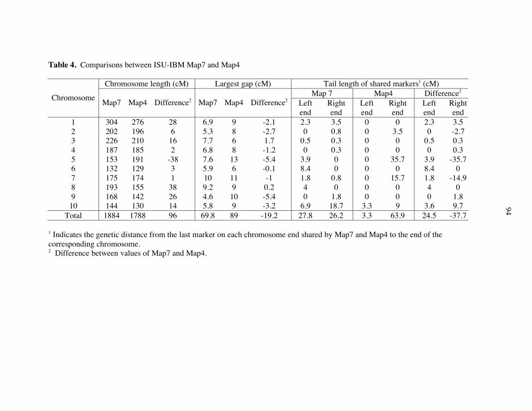
Table 4. Comparisons between ISU-IBM Map7 and Map4
Chromosome length (cM) Largest gap (cM) Tail length of shared markers1 (cM) Map 7 Map4 Difference2 Chromosome Map7 Map4 Difference2 Map7 Map4 Difference2 Left
end Right end
Left end
Right end
Left end
Right end
1 304 276 28 6.9 9 -2.1 2.3 3.5 0 0 2.3 3.5 2 202 196 6 5.3 8 -2.7 0 0.8 0 3.5 0 -2.7 3 226 210 16 7.7 6 1.7 0.5 0.3 0 0 0.5 0.3 4 187 185 2 6.8 8 -1.2 0 0.3 0 0 0 0.3 5 153 191 -38 7.6 13 -5.4 3.9 0 0 35.7 3.9 -35.7 6 132 129 3 5.9 6 -0.1 8.4 0 0 0 8.4 0 7 175 174 1 10 11 -1 1.8 0.8 0 15.7 1.8 -14.9 8 193 155 38 9.2 9 0.2 4 0 0 0 4 0 9 168 142 26 4.6 10 -5.4 0 1.8 0 0 0 1.8 10 144 130 14 5.8 9 -3.2 6.9 18.7 3.3 9 3.6 9.7
Total 1884 1788 96 69.8 89 -19.2 27.8 26.2 3.3 63.9 24.5 -37.7 1 Indicates the genetic distance from the last marker on each chromosome end shared by Map7 and Map4 to the end of the corresponding chromosome. 2 Difference between values of Map7 and Map4.
94

Table 5. The genetic, physical and rice synteny locations of gap flanking and gap filling markers
ISU-IBM Map7 BAC/BAC contig Chr Marker
source Marker
ID
Map4 location
(cM) Chr Marker type3
Location (cM)
Accession No. Contig4 Anchored
Chr Rice locus5
Fill in the
expected location?
IDP806 248 1 sk 271.8 - - - Os03g58480 - Gap flanking1 IDP772 256.5 1 mu 281.5 - - - Os03g60950 -
IDP7387 -6 1 mu 294.5 - - - Os03g62740 Yes IDP7909 - 1 sk 299.1 AC186520 66 1 Os03g63280 Yes IDP7902 - 5 sk 2.1 - - - Os03g62690 No
Gap filling2
IDP8017 - 7 mu 100.8 AC195981 326 8 Os03g62790 No IDP626 274.3 1 sk 299.9 AC177870 66 1 Os03g63400 -
1
Gap flanking IDP3920 274.3 1 sk 301.1 AC191423 66 1 Os03g63700 -
1 Markers flanking the largest gaps on ISU-IBM Map4 2 Markers designed to filling in the largest gaps on ISU-IBM Map4 3 sk – skeleton marker; mu – muscle marker 4 BAC contig assembled by AGI 5 Physical position in The Institute for Genomic Research’s (TIGR’s) release 3.0 of the rice genome (http://www.tigr.org/tdb/e2k1/osa1/pseudomolecules) 6 Data not available
95

Table 5. (continued) ISU-IBM Map7 BAC/BAC contig
Chr Marker source
Marker ID
Map4 location
(cM) Chr Marker type
Location (cM)
Accession No. Contig Anchored
Chr Rice locus
Fill in the
expected location?
IDP233 152.7 5 mu 150.3 - - - Os02g49330 - Gap flanking IDP2474 155.3 - - - - - - Os02g49840 -
IDP7908 - 1 sk 72.6 - - - Os02g51880 No IDP7907 - 3 mu 86.5 - - - Os02g52780 No IDP7898 - 4 sk 113.9 AC185668 182 4 Os02g53520 No IDP7911 - 4 mu 115.3 - - Os02g52670 No IDP8018 - 4 sk 115.6 AC183914 182 4 Os02g52740 No IDP7912 - 4 sk 115.9 AC183914 182 4 Os02g52550 No IDP7899 - 4 sk 117.1 AC185627 182 4 Os02g52180 No IDP7504 - 4 sk 121.4 AC185478 182 4 Os02g51480 No IDP7901 - 4 sk 121.7 AC185478 182 4 Os02g51440 No IDP7900 - 8 mu 149.5 AC155590 253 5 Os02g52610 No
Gap filling
IDP7905 - 8 mu 149.5 - - - Os02g52850 No IDP1491 171.4 - - - - - - Os02g54080 -
5
Gap flanking IDP4002 175.3 - - - - - - Os02g54640 -
IDP3822 121 7 sk 134.7 AC194977 323 7 Os07g38590 - Gap flanking IDP1981 122.5 7 mu 136.5 - - - Os07g38960 -
IDP7913 - 7 sk 137.7 - - - Os07g39310 Yes IDP7252 - 7 sk 139.5 AC197343 323 7 Os07g39810 Yes
7 Gap
filling IDP7184 - 2 sk 144.6 - - - Os07g39980 No
Gap IDP1960 136.5 7 sk 148.1 - - - Os07g4097 -
96

Table 5. (continued) ISU-IBM Map7 BAC/BAC contig
Chr
Marker source
Marker ID
Map4 location
(cM) Chr Marker type
Location (cM)
Accession No. Contig Anchored
Chr Rice locus
Fill in the
expected location?
7 flanking IDP657 158 7 sk 171.3 - - - Os07g4418 - IDP63 94.1 9 sk 108.4 - - - Os03g15050 - Gap
flanking IDP3826 94.1 9 mu 108.4 - - - Os03g14370 - IDP6028 - 9 sk 114.1 - - - Os03g13550 Yes IDP8021 - 9 sk 121.9 - - - Os03g12510 Yes IDP7904 - 1 sk 72.3 - - - Os03g12630 No IDP7583 - 1 sk 72.3 - - - Os03g12620 No IDP7238 - 1 mu 72.3 AC197594 9 1 Os03g12890 No
Gap filling
IDP6029 - 1 sk 76.8 - - - Os03g14260 No IDP493 105.1 9 sk 121.9 - - - Os03g12500 -
9
Gap flanking IDP549 108.9 9 sk 127 - - - Os03g11610 -
97 97

98
Table 6. Comparisons of genetic distances between one pair of markers per chromosomes in FIBC and IBM IRIL mapping populations
Chr
No. scored spots
No. recombined
spots Recombination
rate (%)
Haldane distance in
F1BC
Genetic distance on
map7 1 287 27 9.4 10 6.8 2 335 9 2.7 2.8 4 3 352 19 5.4 5.7 4.4 4 330 22 6.7 7.2 5.9 5 330 18 5.4 5.8 6.3 6 339 44 7.9 8.6 8 7 294 11 3.7 3.9 7.9 8 308 24 7.8 8.5 6.1 9 318 35 11 12.4 7.1
10 309 37 12 13.7 10.5

99
Table 7. Number of markers within QTL intervals on the IBM2 and ISU-IBM Map7 genetic maps and the numbers of sequenced BACs associated with the ISU-IBM Map7 intervals
No. markers in QTL region QTL1 Flanking markers1 Chr IBM2 Map7 No. BACs2
1 php20537-ufg33 1 3 - - 2 umc1824-bnl2g277 2 7 66 28 3 mmp144-mmp36 3 3 35 20 4 bnlg1816-umc1920 3 13 72 28 5 mmp9-umc1449 3 3 23 5 6 umc1167-psr119a 3 5 42 18 7 lim446-php10025 4 3 60 23 8 umc1155-nbp35 5 3 18 15 9 bnlg1174-phi078 6 - 16 4
10 bnl5.09a-bnl14.28 9 5 - - 11 umc1789-umc1675 9 5 11 4 12 psb527d-umc1053 10 - 30 6 13 psb365a-umc1993 10 4 26 10
1 QTL intervals were reported by (HAZEN et al. 2003) 2 Number of sequenced BACs linked to the QTL interval through ISU IDP markers

100
Table 8. Kolmogorov-Smirnov (K-S) tests on the distributions of strongly and weakly expressed genes
Chr No. Low1 No. High2 P-value3 1 110 69 5.80E-06* 2 82 41 0.0391* 3 86 52 0.0237* 4 72 45 0.0390* 5 70 29 0.0711 6 72 46 0.0005* 7 48 44 3.78E-05* 8 53 18 0.9690 9 41 34 0.1263
10 60 50 0.0019* Total 694 428 -
1 Number of mapped genes in the lowest 25th percentile based on expression level. 2 Number of mapped genes in the highest 25th percentile based on expression level. 3 P-value from Kolmogorov-Smirnov (K-S) test; * indicates significant at the 0.05 level.

101
Figure 2. Density plots of strongly and weakly genes on chromosomes 1-10. Genes that are included in the bottom and top 25th percentiles are plotted in blue and green respectively. The numbers of genes plotted for each chromosome are presented in Table 8. Vertical line indicates the position of the centromere.

102

103

104
Supplementary Data Table 1. Anchoring information for all BAC FPCs
Contig id Chr1 Pos2
No. of markers3 Anchoring information4
Cate-gory5
Ctg1 1 0.6 4 Chr1:4:3-sk_ISU:1-mu_MMP #4
Ctg2 1 3.8 9 Chr1:8:6-sk_ISU:2-sk_MMP Chr10:1:1-mu_ISU #3
Ctg3 1 15.1 14 Chr1:14:10-sk_ISU:2-mu_ISU:2-mu_MMP #4
Ctg4 1 29.4 34 Chr8:2:2-mu_ISU Chr1:32:15-sk_ISU:12-mu_ISU:2-sk_MMP:3-mu_MMP #3
Ctg5 1 40.7 12
Chr1:6:5-sk_ISU:1-sk_MMP Chr3:3:2-sk_ISU:1-mu_ISU Chr7:1:1-sk_ISU Chr9:1:1-sk_ISU Chr2:1:1-sk_ISU #3
Ctg6 1 47.8 4 Chr1:3:1-sk_ISU:1-mu_ISU:1-mu_MMP Chr9:1:1-mu_MMP #3
Ctg7 - - 2 Chr1:1:1-mu_ISU Chr9:1:1-sk_ISU #2
Ctg8 1 54.2 12
Chr1:10:1-sk_ISU:6-mu_ISU:2-umapit_ISU:1-sk_MMP Chr3:1:1-sk_ISU Chr9:1:1-mu_ISU #3
Ctg9 1 67.2 19
Chr1:15:7-sk_ISU:7-mu_ISU:1-sk_MMP Chr3:2:2-sk_ISU Chr9:2:1-sk_ISU:1-sk_MMP #3
Ctg10 1 72.6 2 Chr1:2:2-mu_ISU #4
Ctg11 1 88.3 20
Chr6:1:1-mu_ISU Chr1:17:11-sk_ISU:2-mu_ISU:2-sk_MMP:2-mu_MMP Chr9:1:1-sk_MMP Chr10:1:1-sk_ISU #3
Ctg12 1 67.8 6 Chr1:6:2-sk_ISU:4-mu_ISU #4 Ctg13 1 101.1 3 Chr1:3:3-sk_ISU #4 Ctg14 1 104.4 11 Chr1:11:7-sk_ISU:3-mu_ISU:1-mu_MMP #4
1 Chromosome to which BAC contig is anchored. 2 Anchored genetic position, which is the average of the genetic position of closely linked markers (≤ 30 cM). 3 Number of markers linked to the BAC contig. 4 The format of the anchoring information is chromosome number:number markers from this chromosome:number markers of each specific type. Marker types type of markers is consist of two parts linked by underscore. sk – skeleton marker, mu – muscle marker, umapit – markers linked to ISU-IBM Map7 using the U-Map-It software, ISU – markers identified by Iowa State University, MMP – markers identified by the Missouri Maize Mapping Project. 5 Categories: #1 - BAC contig was hit by one marker; #2 – BAC contig hit by multiple non-closely linked and inconsistent markers; #3- BAC contig hit by multiple markers and majority of those markers were closely linked; #4 – BAC contig hit by multiple closely linked markers.

105
Table 1. (continued) Contig
id Chr Pos No. of
markers Anchoring information Cate-gory
Ctg15 1 140.6 4 Chr1:4:2-sk_ISU:2-mu_ISU #4 Ctg17 - - 1 Chr1:1:1-mu_ISU #1 Ctg18 1 115.6 3 Chr1:3:1-sk_ISU:2-mu_ISU #4 Ctg19 1 118.1 4 Chr1:4:2-sk_ISU:2-mu_ISU #4
Ctg20 1 142.4 5 Chr1:4:2-sk_ISU:2-mu_ISU Chr2:1:1-mu_MMP #3
Ctg21 1 122.5 5 Chr1:5:4-sk_ISU:1-mu_ISU #4 Ctg22 1 122.9 3 Chr1:3:2-sk_ISU:1-mu_ISU #4
Ctg23 1 124.7 9
Chr1:7:1-sk_ISU:5-mu_ISU:1-mu_MMP Chr4:1:1-mu_ISU Chr9:1:1-sk_ISU #3
Ctg24 1 126.1 2 Chr1:2:2-sk_ISU #4 Ctg25 1 125.1 2 Chr1:2:2-sk_ISU #4 Ctg27 1 129.6 3 Chr1:2:2-mu_ISU Chr2:1:1-sk_ISU #3
Ctg28 1 128.6 5 Chr6:1:1-mu_ISU Chr1:4:2-sk_ISU:2-mu_ISU #3
Ctg29 1 129.8 3 Chr1:3:2-sk_ISU:1-sk_MMP #4
Ctg30 1 145.8 9
Chr8:1:1-sk_ISU Chr1:5:2-sk_ISU:1-mu_ISU:1-sk_MMP:1-mu_MMP Chr10:1:1-mu_ISU Chr5:2:2-sk_ISU #3
Ctg31 1 130.8 9 Chr1:6:4-sk_ISU:2-mu_ISU Chr9:3:2-sk_ISU:1-mu_ISU #3
Ctg32 1 130.8 6 Chr1:6:6-mu_ISU #4 Ctg33 1 132.6 1 Chr1:1:1-sk_ISU #4
Ctg34 1 132.9 3 Chr1:3:2-umapit_ISU:1-umapit_MMP #4
Ctg35 1 133.8 4 Chr1:4:1-mu_ISU:2-umapit_ISU:1-umapit_MMP #4
Ctg36 1 135.9 11 Chr1:11:4-sk_ISU:2-mu_ISU:5-umapit_ISU #4
Ctg37 1 139.6 18 Chr1:17:7-sk_ISU:8-mu_ISU:2-mu_MMP Chr4:1:1-sk_ISU #3
Ctg38 1 150.4 7
Chr1:5:1-sk_ISU:2-mu_ISU:1-sk_MMP:1-mu_MMP Chr3:1:1-mu_MMP Chr2:1:1-sk_ISU #3
Ctg39 1 154.8 5 Chr1:4:3-sk_ISU:1-umapit_MMP Chr10:1:1-mu_MMP #3
Ctg41 1 164.5 19 Chr1:19:5-sk_ISU:11-mu_ISU:3-mu_MMP #4

106
Table 1. (continued) Contig
id Chr Pos No. of
markers Anchoring information Cate-gory
Ctg42 1 179 4 Chr1:4:4-mu_ISU #4 Ctg43 1 179.8 10 Chr1:10:8-sk_ISU:2-mu_ISU #4 Ctg44 1 190.3 15 Chr1:15:8-sk_ISU:7-mu_ISU #4 Ctg45 1 200.7 2 Chr1:2:1-sk_ISU:1-mu_MMP #4
Ctg46 1 205.8 9 Chr1:9:3-sk_ISU:4-mu_ISU:1-sk_MMP:1-mu_MMP #4
Ctg47 1 209.5 3 Chr1:2:1-sk_ISU:1-mu_ISU Chr4:1:1-mu_ISU #3
Ctg48 1 183.1 5 Chr1:5:5-sk_ISU #4
Ctg49 1 214.6 16
Chr6:1:1-sk_ISU Chr8:1:1-mu_ISU Chr1:13:6-sk_ISU:4-mu_ISU:1-umapit_ISU:2-mu_MMP Chr5:1:1-umapit_MMP #3
Ctg50 1 221.4 7 Chr1:7:4-sk_ISU:2-mu_ISU:1-mu_MMP #4
Ctg51 1 228 1 Chr1:1:1-sk_ISU #4
Ctg52 1 225.8 6
Chr1:3:2-sk_ISU:1-mu_MMP Chr3:3:1-sk_ISU:1-mu_ISU:1-umapit_MMP #3
Ctg53 2 98.3 4 Chr2:4:3-sk_ISU:1-mu_ISU #4 Ctg54 1 234.1 3 Chr1:3:3-sk_ISU #4
Ctg55 4 139.3 7
Chr4:4:2-sk_ISU:1-mu_ISU:1-mu_MMP Chr1:3:2-sk_ISU:1-mu_ISU #3
Ctg56 1 235 5 Chr1:4:1-sk_ISU:3-mu_ISU Chr3:1:1-sk_ISU #3
Ctg57 1 241.8 33
Chr6:2:2-mu_ISU Chr1:22:9-sk_ISU:8-mu_ISU:2-umapit_ISU:3-mu_MMP Chr3:6:4-sk_ISU:1-mu_ISU:1-mu_MMP Chr7:1:1-umapit_MMP Chr9:1:1-mu_ISU Chr2:1:1-umapit_MMP #3
Ctg58 1 212.1 6 Chr1:4:1-sk_ISU:2-mu_ISU:1-umapit_ISU Chr5:2:2-sk_ISU #3
Ctg59 1 254.5 6 Chr1:6:5-sk_ISU:1-mu_ISU #4 Ctg60 1 256.5 4 Chr1:4:3-sk_ISU:1-mu_ISU #4 Ctg61 1 260.8 5 Chr1:5:4-sk_ISU:1-mu_ISU #4 Ctg62 1 267.7 3 Chr1:3:3-sk_ISU #4
Ctg63 1 271.4 9 Chr1:9:4-sk_ISU:1-mu_ISU:1-sk_MMP:3-mu_MMP #4

107
Table 1. (continued) Contig
id Chr Pos No. of
markers Anchoring information Cate-gory
Ctg64 1 273.9 7 Chr1:6:3-sk_ISU:2-mu_ISU:1-mu_MMP Chr2:1:1-sk_ISU #3
Ctg65 1 290.7 7 Chr1:6:4-sk_ISU:1-mu_ISU:1-mu_MMP Chr5:1:1-mu_MMP #3
Ctg66 1 300.3 14 Chr1:14:10-sk_ISU:1-mu_ISU:3-mu_MMP #4
Ctg67 1 303.6 2 Chr1:2:1-sk_ISU:1-mu_ISU #4
Ctg68 2 6.4 20
Chr1:1:1-mu_ISU Chr3:1:1-mu_ISU Chr10:1:1-mu_MMP Chr2:17:13-sk_ISU:2-mu_ISU:1-mu_MMP:1-umapit_MMP #3
Ctg69 2 21.1 11 Chr2:11:3-sk_ISU:5-mu_ISU:2-mu_MMP:1-umapit_MMP #4
Ctg70 2 31.5 23 Chr10:1:1-sk_ISU Chr2:22:6-sk_ISU:13-mu_ISU:3-mu_MMP #3
Ctg71 2 52.8 13 Chr8:1:1-mu_ISU Chr2:12:7-sk_ISU:4-mu_ISU:1-sk_MMP #3
Ctg72 2 52.5 6 Chr2:6:4-sk_ISU:1-mu_ISU:1-sk_MMP #4
Ctg73 2 55.5 7 Chr10:1:1-mu_MMP Chr2:6:3-sk_ISU:3-mu_ISU #3
Ctg74 2 75.2 18
Chr10:3:2-sk_ISU:1-mu_ISU Chr2:15:9-sk_ISU:5-mu_ISU:1-mu_MMP #3
Ctg75 2 79.2 2 Chr2:2:2-mu_ISU #4
Ctg76 2 81.8 14
Chr10:3:1-mu_ISU:2-umapit_MMP Chr2:11:3-sk_ISU:4-mu_ISU:1-sk_MMP:2-mu_MMP:1-umapit_MMP #3
Ctg77 2 84.2 6 Chr2:6:4-sk_ISU:1-mu_ISU:1-sk_MMP #4
Ctg78 2 88.6 14 Chr1:2:2-sk_ISU Chr2:12:6-sk_ISU:5-mu_ISU:1-mu_MMP #3
Ctg79 2 96.1 10 Chr6:1:1-mu_ISU Chr2:9:1-sk_ISU:7-mu_ISU:1-mu_MMP #3
Ctg80 2 100.1 2 Chr2:2:1-sk_ISU:1-mu_MMP #4
Ctg82 2 97.8 8
Chr6:1:1-mu_ISU Chr3:1:1-sk_ISU Chr10:1:1-sk_ISU Chr9:1:1-mu_ISU Chr2:4:1-sk_ISU:2-mu_ISU:1-sk_MMP #3

108
Table 1. (continued) Contig
id Chr Pos No. of
markers Anchoring information Cate-gory
Ctg84 10 43.7 6 Chr10:5:3-sk_ISU:2-mu_ISU Chr2:1:1-sk_ISU #3
Ctg85 2 102.4 3 Chr2:3:1-sk_ISU:2-mu_ISU #4
Ctg86 2 102.5 13
Chr1:2:1-sk_ISU:1-sk_MMP Chr2:11:2-sk_ISU:8-mu_ISU:1-sk_MMP #3
Ctg87 - - 2 Chr4:1:1-sk_ISU Chr2:1:1-mu_ISU #2
Ctg88 - - 2 Chr8:1:1-mu_ISU Chr2:1:1-mu_ISU #2
Ctg89 2 104.6 9
Chr1:1:1-mu_MMP Chr2:7:4-sk_ISU:2-mu_ISU:1-mu_MMP Chr5:1:1-sk_ISU #3
Ctg90 2 105.3 5 Chr4:1:1-sk_ISU Chr2:4:1-sk_ISU:3-mu_ISU #3
Ctg91 2 109.6 11
Chr7:2:1-mu_MMP:1-umapit_MMP Chr2:9:3-sk_ISU:5-mu_ISU:1-umapit_ISU #3
Ctg92 2 112.6 7 Chr1:1:1-mu_MMP Chr2:6:3-mu_ISU:3-sk_MMP #3
Ctg93 - - 1 Chr2:1:1-sk_ISU #1 Ctg94 2 112.5 2 Chr2:2:2-sk_ISU #4 Ctg95 - - 1 Chr2:1:1-sk_ISU #1 Ctg96 2 112.9 2 Chr2:2:1-sk_ISU:1-mu_ISU #4 Ctg97 - - 1 Chr4:1:1-mu_ISU #1 Ctg98 2 118.7 13 Chr2:13:8-sk_ISU:5-mu_ISU #4 Ctg99 2 120.9 3 Chr2:3:3-mu_ISU #4 Ctg100 2 123.4 2 Chr2:2:1-sk_ISU:1-mu_ISU #4 Ctg101 - - 1 Chr2:1:1-sk_ISU #1 Ctg102 2 128.8 5 Chr2:5:1-sk_ISU:4-mu_ISU #4
Ctg103 2 134.6 20
Chr8:1:1-sk_ISU Chr1:2:1-mu_ISU:1-mu_MMP Chr3:1:1-mu_ISU Chr7:1:1-mu_ISU #3
Ctg104 2 151.4 10
Chr1:1:1-sk_ISU Chr2:9:4-sk_ISU:4-mu_ISU:1-umapit_MMP #3
Ctg105 2 160.9 6 Chr2:6:2-sk_ISU:4-mu_ISU #4 Ctg106 9 65.2 4 Chr9:4:4-mu_ISU #4 Ctg107 2 166.7 4 Chr2:4:3-sk_ISU:1-sk_MMP #4 Ctg108 2 172 14 Chr2:14:13-sk_ISU:1-mu_ISU #4

109
Table 1. (continued) Contig
id Chr Pos No. of
markers Anchoring information Cate-gory
Ctg109 2 191.5 6 Chr3:1:1-sk_ISU Chr2:5:2-sk_ISU:3-mu_ISU #3
Ctg110 2 199.4 4 Chr7:1:1-mu_MMP Chr10:1:1-mu_ISU Chr2:2:2-sk_ISU #3
Ctg111 3 17.3 25
Chr6:3:2-sk_ISU:1-mu_ISU Chr3:22:9-sk_ISU:5-mu_ISU:1-umapit_ISU:2-sk_MMP:5-mu_MMP #3
Ctg112 3 45.4 3 Chr3:3:3-sk_ISU #4
Ctg114 3 65.7 5 Chr3:5:1-sk_ISU:1-mu_ISU:1-sk_MMP:2-mu_MMP #4
Ctg115 3 72.4 11 Chr1:1:1-sk_ISU Chr3:10:5-sk_ISU:3-mu_ISU:2-mu_MMP #3
Ctg116 3 74.6 5 Chr3:5:3-sk_ISU:1-sk_MMP:1-mu_MMP #4
Ctg117 3 77.8 32
Chr8:2:1-sk_ISU:1-sk_MMP Chr3:30:14-sk_ISU:13-mu_ISU:1-sk_MMP:1-mu_MMP:1-umapit_MMP #3
Ctg118 3 80.3 23
Chr1:5:5-mu_ISU Chr4:2:2-mu_ISU Chr3:9:2-sk_ISU:6-mu_ISU:1-mu_MMP Chr7:1:1-mu_ISU Chr10:4:3-sk_ISU:1-mu_ISU Chr5:2:1-sk_ISU:1-mu_ISU #3
Ctg119 3 82.2 7
Chr3:6:4-mu_ISU:1-umapit_ISU:1-mu_MMP Chr9:1:1-mu_MMP #3
Ctg120 3 82.4 2 Chr3:2:2-mu_ISU #4
Ctg121 3 84.4 10
Chr1:2:1-sk_ISU:1-mu_MMP Chr3:7:4-sk_ISU:3-mu_ISU Chr10:1:1-sk_ISU #3
Ctg122 - - 1 Chr1:1:1-sk_MMP #1
Ctg123 3 85.9 10 Chr3:9:2-sk_ISU:6-mu_ISU:1-mu_MMP Chr7:1:1-sk_ISU #3
Ctg124 3 90.6 18
Chr1:1:1-sk_ISU Chr3:12:4-sk_ISU:8-mu_ISU Chr10:1:1-mu_MMP Chr2:4:1-sk_ISU:3-mu_ISU #3
Ctg125 3 92.5 4 Chr3:4:1-sk_ISU:3-mu_ISU #4 Ctg126 3 96.1 4 Chr3:4:4-sk_ISU #4 Ctg127 4 141 4 Chr4:4:1-sk_ISU:3-mu_ISU #4

110
Table 1. (continued) Contig
id Chr Pos No. of
markers Anchoring information Cate-gory
Ctg128 3 97.4 9
Chr3:8:3-sk_ISU:3-mu_ISU:1-mu_MMP:1-umapit_MMP Chr2:1:1-sk_ISU #3
Ctg129 3 101.6 1 Chr3:1:1-mu_ISU #4 Ctg131 3 106.5 4 Chr3:4:2-sk_ISU:2-mu_ISU #4
Ctg132 3 114.7 17
Chr8:1:1-sk_ISU Chr3:16:4-sk_ISU:6-mu_ISU:5-mu_MMP:1-umapit_MMP #3
Ctg134 3 123.7 6 Chr3:6:3-sk_ISU:3-mu_ISU #4 Ctg135 3 88.5 2 Chr3:2:1-sk_ISU:1-umapit_ISU #4
Ctg136 3 133.3 8 Chr3:8:4-sk_ISU:3-mu_ISU:1-mu_MMP #4
Ctg137 3 133.3 5 Chr1:1:1-mu_ISU Chr3:4:2-sk_ISU:2-mu_ISU #3
Ctg138 3 147.3 13 Chr3:12:5-sk_ISU:4-mu_ISU:3-mu_MMP Chr9:1:1-sk_ISU #3
Ctg139 3 152.8 6 Chr1:1:1-sk_ISU Chr3:5:4-mu_ISU:1-mu_MMP #3
Ctg140 3 152.8 2 Chr3:2:1-sk_ISU:1-mu_ISU #4
Ctg141 3 153.6 7 Chr3:7:4-sk_ISU:1-mu_ISU:1-sk_MMP:1-mu_MMP #4
Ctg142 3 160.7 10
Chr8:1:1-mu_ISU Chr3:9:2-sk_ISU:4-mu_ISU:1-sk_MMP:1-mu_MMP:1-umapit_MMP #3
Ctg143 3 165.3 3 Chr3:3:3-sk_ISU #4 Ctg144 - - 1 Chr3:1:1-sk_ISU #1
Ctg145 3 173.7 7 Chr3:6:4-sk_ISU:2-mu_ISU Chr10:1:1-sk_ISU #3
Ctg146 3 186.9 7 Chr3:7:5-sk_ISU:1-sk_MMP:1-mu_MMP #4
Ctg147 3 190.8 2 Chr3:2:1-sk_ISU:1-mu_ISU #4
Ctg148 3 191.8 10 Chr1:1:1-mu_ISU Chr3:9:7-sk_ISU:2-mu_ISU #3
Ctg149 3 199.5 11 Chr3:11:3-sk_ISU:5-mu_ISU:3-mu_MMP #4
Ctg150 3 208.5 14 Chr6:1:1-mu_ISU Chr3:13:7-sk_ISU:6-mu_ISU #3
Ctg151 3 221.5 23
Chr8:1:1-sk_ISU Chr3:21:13-sk_ISU:8-mu_ISU Chr2:1:1-mu_ISU #3
Ctg152 - - 1 Chr3:1:1-mu_ISU #1

111
Table 1. (continued) Contig
id Chr Pos No. of
markers Anchoring information Cate-gory
Ctg153 3 226.1 3 Chr3:3:2-sk_ISU:1-sk_MMP #4 Ctg154 4 0.4 3 Chr4:3:2-sk_ISU:1-mu_MMP #4
Ctg155 4 10.5 11 Chr4:9:2-sk_ISU:7-mu_ISU Chr10:2:2-mu_ISU #3
Ctg156 4 20.3 4 Chr4:4:2-sk_ISU:2-mu_ISU #4 Ctg157 4 38.3 3 Chr4:3:1-sk_ISU:2-mu_ISU #4
Ctg158 4 51.4 6 Chr4:6:3-sk_ISU:1-mu_ISU:2-mu_MMP #4
Ctg159 4 57.6 3 Chr4:3:2-mu_ISU:1-mu_MMP #4
Ctg160 4 63.4 11 Chr4:10:3-sk_ISU:7-mu_ISU Chr5:1:1-sk_ISU #3
Ctg161 - - 1 Chr3:1:1-mu_ISU #1
Ctg162 4 73.1 8 Chr8:1:1-sk_ISU Chr4:7:2-sk_ISU:4-mu_ISU:1-mu_MMP #3
Ctg163 4 74.6 9 Chr4:7:7-mu_ISU Chr10:2:1-sk_ISU:1-sk_MMP #3
Ctg164 4 76.5 26
Chr6:2:2-mu_ISU Chr1:2:1-mu_ISU:1-sk_MMP Chr4:19:6-sk_ISU:13-mu_ISU Chr3:1:1-mu_ISU Chr7:1:1-mu_ISU Chr5:1:1-sk_ISU #3
Ctg165 4 82.7 2 Chr4:2:2-mu_ISU #4
Ctg166 4 82.5 4 Chr4:3:1-mu_ISU:2-mu_MMP Chr3:1:1-sk_ISU #3
Ctg168 4 84.3 4 Chr4:3:2-sk_ISU:1-mu_ISU Chr1:1:1-sk_ISU #3
Ctg170 4 84.5 2 Chr4:2:2-mu_ISU #4
Ctg171 - - 2 Chr4:1:1-mu_ISU Chr5:1:1-sk_ISU #2
Ctg172 4 83.4 7 Chr4:6:3-sk_ISU:3-mu_ISU Chr9:1:1-sk_ISU #3
Ctg173 - - 1 Chr4:1:1-sk_ISU #1 Ctg174 - - 1 Chr9:1:1-mu_ISU #1 Ctg176 4 84.5 9 Chr4:9:2-sk_ISU:7-mu_ISU #4 Ctg179 4 87.2 8 Chr4:8:1-sk_ISU:7-mu_ISU #4
Ctg181 4 95.3 20
Chr4:16:9-sk_ISU:6-mu_ISU:1-mu_MMP Chr10:1:1-sk_ISU Chr5:3:1-sk_ISU:1-sk_MMP:1-mu_MMP #3

112
Table 1. (continued) Contig
id Chr Pos No. of
markers Anchoring information Cate-gory
Ctg182 4 110.5 53
Chr4:43:25-sk_ISU:14-mu_ISU:1-umapit_ISU:2-mu_MMP:1-umapit_MMP Chr1:2:1-sk_ISU:1-mu_ISU Chr3:1:1-sk_ISU Chr9:1:1-mu_ISU Chr5:6:1-sk_ISU:2-mu_ISU:1-umapit_ISU:1-sk_MMP:1-mu_MMP #3
Ctg184 4 127.7 6 Chr6:1:1-mu_ISU Chr4:5:3-sk_ISU:1-mu_ISU:1-mu_MMP #3
Ctg185 - - 1 Chr4:1:1-sk_ISU #1 Ctg186 4 128 1 Chr4:1:1-sk_ISU #4 Ctg187 - - 1 Chr4:1:1-sk_ISU #1
Ctg188 4 134.1 10
Chr4:9:4-sk_ISU:3-mu_ISU:1-mu_MMP:1-umapit_MMP Chr2:1:1-sk_ISU #3
Ctg189 4 141.9 3 Chr4:3:3-mu_ISU #4 Ctg190 4 80 4 Chr4:4:4-mu_ISU #4 Ctg191 4 135.7 5 Chr4:5:4-mu_ISU:1-mu_MMP #4 Ctg192 - - 1 Chr4:1:1-mu_ISU #1
Ctg193 4 138.4 5
Chr8:1:1-mu_ISU Chr4:3:1-sk_ISU:1-mu_ISU:1-sk_MMP Chr9:1:1-sk_ISU #3
Ctg194 4 135.9 4 Chr4:4:2-sk_ISU:2-mu_ISU #4 Ctg195 4 139.4 1 Chr4:1:1-sk_ISU #4
Ctg197 9 65.2 4 Chr4:1:1-mu_ISU Chr9:3:2-sk_ISU:1-mu_ISU #3
Ctg198 4 149.5 6 Chr4:6:1-sk_ISU:3-mu_ISU:1-sk_MMP:1-mu_MMP #4
Ctg199 4 146.4 7 Chr4:6:5-sk_ISU:1-mu_ISU Chr5:1:1-mu_MMP #3
Ctg200 4 152.1 7 Chr4:7:6-sk_ISU:1-mu_ISU #4
Ctg201 4 169.2 18
Chr4:17:5-sk_ISU:10-mu_ISU:1-sk_MMP:1-mu_MMP Chr3:1:1-mu_ISU #3
Ctg202 4 180.8 9 Chr4:9:5-sk_ISU:2-mu_ISU:2-mu_MMP #4
Ctg203 4 186.7 2 Chr4:2:1-sk_ISU:1-mu_ISU #4
Ctg204 5 9.6 48
Chr1:1:1-mu_MMP Chr10:1:1-mu_MMP Chr5:46:19-sk_ISU:18-mu_ISU:3- #3
Ctg205 5 24.7 5 Chr5:5:2-sk_ISU:3-mu_ISU #4

113
Table 1. (continued) Contig
id Chr Pos No. of
markers Anchoring information Cate-gory
Ctg206 5 36 9 Chr1:1:1-sk_MMP Chr5:8:5-sk_ISU:3-mu_ISU #3
Ctg207 5 44.3 2 Chr5:2:2-sk_ISU #4 Ctg208 5 45.9 4 Chr5:4:3-sk_ISU:1-sk_MMP #4 Ctg209 5 57.3 8 Chr5:8:6-sk_ISU:2-mu_ISU #4 Ctg210 5 61.8 6 Chr5:6:5-sk_ISU:1-mu_ISU #4
Ctg211 5 71 10 Chr5:10:5-sk_ISU:4-mu_ISU:1-sk_MMP #4
Ctg212 5 73.2 5 Chr5:5:3-sk_ISU:2-mu_ISU #4 Ctg213 5 75.1 1 Chr5:1:1-mu_ISU #4
Ctg215 5 76.9 6 Chr5:6:2-sk_ISU:3-mu_ISU:1-umapit_MMP #4
Ctg216 5 77.1 7 Chr5:7:1-sk_ISU:6-mu_ISU #4
Ctg217 5 79 10
Chr6:2:2-sk_ISU Chr1:1:1-mu_MMP Chr5:7:4-sk_ISU:1-mu_ISU:1-mu_MMP:1-umapit_MMP #3
Ctg218 5 80 4 Chr1:1:1-sk_ISU Chr5:3:2-mu_ISU:1-sk_MMP #3
Ctg219 5 82.7 6 Chr6:1:1-sk_MMP Chr5:5:3-mu_ISU:2-mu_MMP #3
Ctg220 5 85.6 17 Chr5:17:7-sk_ISU:9-mu_ISU:1-mu_MMP #4
Ctg221 - - 1 Chr5:1:1-sk_ISU #1
Ctg223 5 88.1 4 Chr5:4:3-sk_ISU:1-umapit_MMP #4
Ctg224 5 88.8 3 Chr5:3:2-sk_ISU:1-mu_ISU #4 Ctg225 5 92.1 4 Chr5:4:3-sk_ISU:1-mu_ISU #4 Ctg229 - - 1 Chr5:1:1-mu_ISU #1
Ctg231 - - 2 Chr1:1:1-sk_ISU Chr3:1:1-mu_ISU #2
Ctg232 - - 1 Chr5:1:1-sk_ISU #1
Ctg233 3 76.1 4 Chr3:3:2-sk_ISU:1-mu_ISU Chr5:1:1-sk_MMP #3
Ctg234 3 79.5 2 Chr3:1:1-sk_ISU Chr5:1:1-mu_MMP #3
Ctg235 5 96.2 5 Chr5:5:2-sk_ISU:2-mu_ISU:1-mu_MMP #4
Ctg236 5 98.3 3 Chr5:3:2-sk_ISU:1-mu_ISU #4 Ctg237 5 101.6 2 Chr5:2:1-mu_ISU:1-mu_MMP #4 Ctg238 5 107.3 5 Chr5:5:4-sk_ISU:1-mu_ISU #4 Ctg239 5 112.1 4 Chr2:1:1-sk_ISU Chr5:3:2-sk #3

114
Table 1. (continued) Contig
id Chr Pos No. of
markers Anchoring information Cate-gory
Ctg240 5 115.3 3 Chr5:3:1-sk_ISU:1-mu_ISU:1-mu_MMP #4
Ctg241 - - 1 Chr5:1:1-mu_ISU #1 Ctg242 5 119.2 16 Chr5:16:14-sk_ISU:2-mu_ISU #4 Ctg243 5 120.6 3 Chr5:3:1-sk_ISU:2-mu_ISU #4 Ctg244 5 121 2 Chr5:2:2-sk_ISU #4
Ctg245 5 126.2 8
Chr4:1:1-mu_MMP Chr2:1:1-mu_ISU Chr5:6:5-sk_ISU:1-mu_ISU #3
Ctg246 - - 1 Chr4:1:1-mu_ISU #1 Ctg247 5 130.1 2 Chr5:2:2-sk_ISU #4 Ctg248 5 137.8 2 Chr5:2:1-mu_ISU:1-mu_MMP #4
Ctg250 5 145.7 16
Chr1:1:1-mu_MMP Chr10:1:1-sk_ISU Chr5:14:12-sk_ISU:1-mu_ISU:1-mu_MMP #3
Ctg251 4 119.1 3 Chr4:2:1-mu_ISU:1-sk_MMP Chr5:1:1-mu_ISU #3
Ctg252 5 152.6 3 Chr5:3:2-sk_ISU:1-umapit_ISU #4
Ctg253 6 108.8 10
Chr6:4:3-mu_ISU:1-umapit_ISU Chr8:2:2-mu_ISU Chr4:1:1-mu_MMP Chr1:2:1-sk_ISU:1-mu_ISU Chr7:1:1-mu_ISU #3
Ctg255 3 82.7 5 Chr6:1:1-umapit_ISU Chr3:4:3-sk_ISU:1-mu_ISU #3
Ctg256 - - 1 Chr6:1:1-mu_ISU #1 Ctg257 6 4 3 Chr6:3:3-mu_ISU #4 Ctg259 - - 1 Chr9:1:1-sk_ISU #1
Ctg260 6 2.6 6 Chr6:5:4-mu_ISU:1-sk_MMP Chr8:1:1-mu_MMP #3
Ctg261 6 4.8 3 Chr6:3:3-mu_ISU #4
Ctg262 6 7.4 6 Chr6:4:4-mu_ISU Chr8:1:1-sk_ISU Chr2:1:1-sk_ISU #3
Ctg263 6 3.7 13 Chr6:12:2-sk_ISU:10-mu_ISU Chr10:1:1-mu_MMP #3
Ctg265 6 8.4 7 Chr6:7:4-sk_ISU:2-mu_ISU:1-mu_MMP #4
Ctg267 6 8.4 4
Chr6:2:1-sk_ISU:1-mu_ISU Chr4:1:1-sk_ISU Chr10:1:1-sk_ISU #3
Ctg268 - - 1 Chr6:1:1-sk_ISU #1 Ctg269 6 8.4 6 Chr6:6:5-sk_ISU:1-sk_MMP #4

115
Table 1. (continued) Contig
id Chr Pos No. of
markers Anchoring information Cate-gory
Ctg270 6 8.7 5
Chr6:3:1-sk_ISU:2-mu_ISU Chr2:2:1-sk_ISU:1-umapit_MMP #3
Ctg271 6 13.6 6 Chr6:6:3-sk_ISU:1-mu_ISU:1-umapit_ISU:1-sk_MMP #4
Ctg272 - - 1 Chr6:1:1-sk_ISU #1 Ctg273 6 19.5 5 Chr6:5:4-sk_ISU:1-mu_ISU #4 Ctg274 6 21.4 6 Chr6:6:1-sk_ISU:5-mu_ISU #4 Ctg275 6 24.8 3 Chr6:3:1-sk_ISU:2-mu_ISU #4
Ctg276 6 28.4 7 Chr6:7:2-sk_ISU:2-mu_ISU:2-mu_MMP:1-umapit_MMP #4
Ctg277 - - 1 Chr6:1:1-sk_ISU #1
Ctg280 6 35.7 3 Chr6:2:1-sk_ISU:1-mu_ISU Chr1:1:1-mu_MMP #3
Ctg281 6 44.6 21
Chr6:20:11-sk_ISU:7-mu_ISU:1-sk_MMP:1-mu_MMP Chr10:1:1-mu_ISU #3
Ctg282 6 51.5 7 Chr6:6:2-sk_ISU:3-mu_ISU:1-umapit_ISU Chr5:1:1-mu_ISU #3
Ctg283 6 53.5 9
Chr6:8:3-sk_ISU:3-mu_ISU:1-sk_MMP:1-umapit_MMP Chr8:1:1-mu_MMP #3
Ctg285 6 61.5 9 Chr6:8:4-sk_ISU:3-mu_ISU:1-mu_MMP Chr8:1:1-sk_ISU #3
Ctg287 6 81.8 12 Chr6:12:8-sk_ISU:3-mu_ISU:1-sk_MMP #4
Ctg288 6 101.4 20
Chr6:18:7-sk_ISU:7-mu_ISU:1-umapit_ISU:1-sk_MMP:2-mu_MMP Chr8:1:1-mu_MMP Chr5:1:1-mu #3
Ctg289 6 121.5 6
Chr8:1:1-mu_MMP Chr6:4:1-sk_ISU:3-mu_ISU Chr4:1:1-mu_ISU #3
Ctg290 6 128.4 8 Chr6:7:4-sk_ISU:2-mu_ISU:1-mu_MMP Chr1:1:1-sk_ISU #3
Ctg291 - - 3 Chr6:1:1-sk_MMP Chr8:1:1-mu_ISU Chr1:1:1-mu_ISU #2
Ctg293 7 8.2 7 Chr7:7:3-sk_ISU:2-mu_ISU:1-mu_MMP:1-umapit_MMP #4
Ctg294 7 42 8 Chr7:8:4-sk_ISU:3-mu_ISU:1-mu_MMP #4
Ctg296 7 60.1 9 Chr7:9:3-sk_ISU:6-mu_ISU #4

116
Table 1. (continued) Contig
id Chr Pos No. of
markers Anchoring information Cate-gory
Ctg298 7 73.6 4 Chr7:4:2-sk_ISU:2-mu_ISU #4 Ctg299 7 75.4 5 Chr7:5:4-sk_ISU:1-mu_ISU #4 Ctg300 7 75.9 8 Chr7:8:8-mu_ISU #4
Ctg301 7 89 8
Chr3:2:1-mu_ISU:1-mu_MMP Chr7:6:1-sk_ISU:4-mu_ISU:1-mu_MMP #3
Ctg304 3 209.8 4 Chr4:1:1-mu_ISU Chr3:3:3-sk_ISU #3
Ctg305 - - 1 Chr7:1:1-mu_ISU #1 Ctg306 - - 1 Chr7:1:1-mu_ISU #1 Ctg307 7 78.4 4 Chr7:4:4-sk_ISU #4
Ctg309 7 80.9 4 Chr7:3:3-sk_ISU Chr2:1:1-mu_ISU #3
Ctg310 7 83.3 6 Chr7:5:2-sk_ISU:2-mu_MMP:1-umapit_MMP Chr2:1:1-mu_ISU #3
Ctg313 7 86.1 5 Chr7:5:3-sk_ISU:2-mu_ISU #4 Ctg314 7 86.9 2 Chr7:2:1-sk_ISU:1-mu_MMP #4
Ctg315 - - 2 Chr8:1:1-mu_ISU Chr7:1:1-sk_ISU #2
Ctg316 - - 1 Chr7:1:1-mu_ISU #1 Ctg317 7 91.9 4 Chr7:4:2-sk_ISU:2-mu_ISU #4
Ctg318 7 101.7 13 Chr4:1:1-mu_MMP Chr7:12:5-sk_ISU:7-mu_ISU #3
Ctg320 7 110.6 17 Chr6:1:1-mu_ISU Chr7:16:5-sk_ISU:9-mu_ISU:2-mu_MMP #3
Ctg321 7 113.6 4 Chr7:4:2-sk_ISU:2-mu_ISU #4
Ctg322 7 117.8 13 Chr7:13:9-sk_ISU:2-mu_ISU:2-sk_MMP #4
Ctg323 7 131.5 20
Chr7:20:12-sk_ISU:6-mu_ISU:1-sk_MMP:1-mu_MMP #4
Ctg324 - - 1 Chr7:1:1-sk_ISU #1
Ctg325 7 162.7 25
Chr6:2:2-sk_ISU Chr4:1:1-mu_ISU Chr7:20:9-sk_ISU:7-mu_ISU:1-sk_MMP:3-mu_MMP Chr2:1:1-mu_ISU Chr5:1:1-mu_ISU #3

117
Table 1. (continued) Contig
id Chr Pos No. of
markers Anchoring information Cate-gory
Ctg326 8 29.5 44
Chr8:40:25-sk_ISU:10-mu_ISU:2-sk_MMP:2-mu_MMP:1-umapit_MMP Chr4:2:1-mu_ISU:1-mu_MMP Chr1:1:1-mu_ISU Chr7:1:1-mu_ISU #3
Ctg327 8 52.3 3 Chr8:3:1-sk_ISU:1-mu_ISU:1-sk_MMP #4
Ctg328 8 55.8 3 Chr8:3:1-sk_ISU:2-mu_ISU #4
Ctg329 8 64.3 13 Chr8:12:8-sk_ISU:4-mu_ISU Chr6:1:1-mu_ISU #3
Ctg331 8 76.5 2 Chr8:2:1-sk_ISU:1-mu_ISU #4 Ctg332 - - 1 Chr8:1:1-mu_ISU #1 Ctg333 - - 1 Chr8:1:1-sk_ISU #1 Ctg334 8 80.1 5 Chr8:5:5-mu_ISU #4 Ctg336 - - 1 Chr6:1:1-sk_MMP #1 Ctg337 8 86.2 1 Chr8:1:1-mu_ISU #4 Ctg338 - - 1 Chr8:1:1-sk_ISU #1 Ctg339 8 82.8 2 Chr8:2:1-sk_ISU:1-mu_ISU #4
Ctg340 8 87.1 6 Chr8:6:3-sk_ISU:2-mu_ISU:1-mu_MMP #4
Ctg341 - - 1 Chr8:1:1-mu_ISU #1 Ctg345 - - 2 Chr8:1:1-sk_ISU Chr7:1:1-mu #2 Ctg347 - - 1 Chr8:1:1-sk_ISU #1 Ctg348 8 94.9 4 Chr8:4:3-sk_ISU:1-mu_ISU #4
Ctg349 8 95.7 8
Chr8:7:2-sk_ISU:3-mu_ISU:1-umapit_ISU:1-umapit_MMP Chr10:1:1-mu_ISU #3
Ctg350 - - 1 Chr8:1:1-mu_ISU #1
Ctg351 8 100.2 10 Chr8:10:5-sk_ISU:4-mu_ISU:1-mu_MMP #4
Ctg353 8 107.1 6 Chr8:6:4-mu_ISU:2-umapit_ISU #4
Ctg354 8 110 19
Chr8:17:3-sk_ISU:11-mu_ISU:3-mu_MMP Chr3:2:2-mu_MMP #3
Ctg355 8 112.3 3 Chr8:3:2-mu_ISU:1-mu_MMP #4 Ctg357 8 114.2 3 Chr8:3:2-sk_ISU:1-mu_ISU #4 Ctg358 3 191.9 2 Chr3:2:2-mu_ISU #4
Ctg360 4 40.3 3 Chr4:1:1-sk_ISU Chr3:1:1-sk_ISU Chr7:1:1-sk_ISU #3
Ctg361 8 124.2 6 Chr8:6:2-mu_ISU:1-sk_MMP:3-mu_MMP #4

118
Table 1. (continued) Contig
id Chr Pos No. of
markers Anchoring information Cate-gory
Ctg362 8 129 22
Chr8:21:10-sk_ISU:10-mu_ISU:1-mu_MMP Chr4:1:1-mu_ISU #3
Ctg363 8 153.3 6 Chr8:5:2-sk_ISU:3-mu_ISU Chr4:1:1-mu_ISU #3
Ctg364 8 164.7 10 Chr8:10:5-sk_ISU:1-mu_ISU:1-sk_MMP:3-mu_MMP #4
Ctg365 8 172.6 5 Chr8:5:4-sk_ISU:1-umapit_MMP #4
Ctg366 8 175.7 4 Chr8:4:2-sk_ISU:1-mu_ISU:1-mu_MMP #4
Ctg367 9 65.2 6 Chr9:6:3-sk_ISU:3-mu_ISU #4
Ctg368 - - 3 Chr6:1:1-sk_MMP Chr9:2:2-sk_ISU #2
Ctg370 9 28.1 4 Chr9:4:1-sk_ISU:3-mu_ISU #4
Ctg371 6 51.6 7
Chr6:4:2-mu_ISU:1-mu_MMP:1-umapit_MMP Chr9:2:1-sk_ISU:1-mu_MMP Chr2:1:1-mu_MMP #3
Ctg372 - - 1 Chr9:1:1-mu_ISU #1
Ctg373 9 54.8 20
Chr9:19:11-sk_ISU:3-mu_ISU:3-mu_MMP:2-umapit_MMP Chr5:1:1-sk_ISU #3
Ctg374 - - 1 Chr9:1:1-mu_ISU #1
Ctg375 9 65.2 2 Chr9:2:1-sk_ISU:1-mu_ISU #4
Ctg376 9 65.8 13
Chr6:1:1-sk_ISU Chr4:1:1-sk_ISU Chr1:3:1-sk_ISU:2-mu_ISU Chr9:8:3-sk_ISU:2-mu_ISU:3-mu_MMP #3
Ctg377 - - 1 Chr9:1:1-mu_ISU #1
Ctg378 - - 1 Chr9:1:1-mu_ISU #1
Ctg380 9 72.1 1 Chr9:1:1-sk_ISU #4
Ctg381 - - 1 Chr9:1:1-sk_ISU #1
Ctg382 1 170.4 2 Chr1:2:2-sk_ISU #4

119
Table 1. (continued) Contig
id Chr Pos No. of
markers Anchoring information Cate-gory
Ctg383 9 77.6 4 Chr9:4:3-sk_ISU:1-mu_ISU #4 Ctg384 9 79.6 4 Chr9:4:2-mu_ISU:2-sk_MMP #4
Ctg385 9 83.8 8
Chr1:1:1-sk_ISU Chr9:6:4-sk_ISU:1-mu_ISU:1-mu_MMP Chr5:1:1-mu_ISU #3
Ctg387 9 93.9 9 Chr4:1:1-sk_ISU Chr9:8:6-sk_ISU:1-mu_ISU:1-sk_MMP #3
Ctg388 9 101.4 2 Chr9:2:2-sk_ISU #4 Ctg389 9 115.8 7 Chr9:7:3-sk_ISU:3-mu_ISU:1-sk #4
Ctg390 9 130 10
Chr1:1:1-sk_MMP Chr9:7:4-sk_ISU:1-mu_ISU:1-mu_MMP:1-umapit_MMP Chr5:2:1-sk_ISU:1-mu_ISU #3
Ctg391 9 154 70
Chr1:4:2-sk_ISU:1-mu_ISU:1-mu_MMP Chr9:64:37-sk_ISU:17-mu_ISU:5-sk_MMP:4-mu_MMP:1-umapit_MMP Chr10:1:1-sk_ISU Chr5:1:1-sk_ISU #3
Ctg392 10 11.3 14
Chr3:1:1-mu_ISU Chr10:13:8-sk_ISU:3-mu_ISU:1-mu_MMP:1-umapit_MMP #3
Ctg393 10 34.5 9
Chr4:1:1-umapit_MMP Chr10:8:3-sk_ISU:4-mu_ISU:1-umapit_ISU #3
Ctg394 10 38.8 4 Chr10:4:2-sk_ISU:2-mu_ISU #4 Ctg395 - - 1 Chr10:1:1-mu_ISU #1 Ctg397 - - 1 Chr10:1:1-mu_ISU #1 Ctg398 - - 1 Chr10:1:1-mu_ISU #1
Ctg399 10 43.5 6 Chr4:1:1-mu_MMP Chr10:5:2-sk_ISU:2-mu_ISU:1-mu_MMP #3
Ctg400 - - 1 Chr10:1:1-mu_MMP #1 Ctg401 10 46 4 Chr10:4:3-sk_ISU:1-mu_ISU #4
Ctg403 10 48.5 8 Chr10:7:4-sk_ISU:3-mu_ISU Chr2:1:1-sk_ISU #3
Ctg404 10 49.4 4 Chr10:4:2-sk_ISU:1-mu_ISU:1-mu_MMP #4
Ctg405 10 50 2 Chr10:2:2-mu_ISU #4 Ctg406 10 50 6 Chr10:6:3-mu_ISU:3-mu_MMP #4
Ctg407 10 50.5 5 Chr10:5:2-sk_ISU:1-mu_ISU:2-mu_MMP #4
Ctg408 - - 1 Chr3:1:1-mu_ISU #1

120
Table 1. (continued) Contig
id Chr Pos No. of
markers Anchoring information Cate-gory
Ctg409 10 52.5 5 Chr10:5:1-sk_ISU:3-mu_ISU:1-mu_MMP #4
Ctg411 10 53.9 4 Chr10:4:2-sk_ISU:2-mu_ISU #4
Ctg412 10 56 6 Chr10:6:1-sk_ISU:3-mu_ISU:2-mu_MMP #4
Ctg413 10 60.4 20 Chr10:19:8-sk_ISU:11-mu_ISU Chr2:1:1-mu_MMP #3
Ctg414 10 69.7 4 Chr10:4:2-sk_ISU:1-mu_ISU:1-mu_MMP #4
Ctg415 10 75.6 12
Chr10:11:5-sk_ISU:5-mu_ISU:1-mu_MMP Chr2:1:1-mu_ISU #3
Ctg416 10 85.3 6 Chr10:5:4-sk_ISU:1-mu_ISU Chr2:1:1-mu_MMP #3
Ctg417 10 96.3 13
Chr6:1:1-mu_MMP Chr1:1:1-mu_ISU Chr4:1:1-sk_ISU Chr10:8:4-sk_ISU:1-mu_ISU:1-umapit_ISU:1-mu_MMP:1-umapit_MMP Chr2:2:2-mu_ISU #3
Ctg418 10 102.5 4 Chr10:4:2-sk_ISU:1-mu_ISU:1-mu_MMP #4
Ctg419 10 120.4 10 Chr10:8:6-sk_ISU:1-mu_ISU:1-mu_MMP Chr2:2:2-sk_ISU #3
Ctg420 - - 1 Chr9:1:1-sk_ISU #1
Ctg421 - - 2 Chr8:1:1-sk_ISU Chr2:1:1-sk_ISU #2
Ctg423 - - 1 Chr10:1:1-mu_ISU #1 Ctg426 - - 1 Chr2:1:1-mu_ISU #1 Ctg428 8 80.5 1 Chr8:1:1-umapit_ISU #1 Ctg430 7 77 2 Chr7:2:2-sk_ISU #4
Ctg432 - - 2 Chr6:1:1-mu_ISU Chr9:1:1-mu_ISU #2
Ctg434 8 69.5 1 Chr8:1:1-mu_MMP #1 Ctg435 - - 1 Chr7:1:1-sk_ISU #1 Ctg438 - - 1 Chr6:1:1-mu_ISU #1 Ctg440 - - 1 Chr6:1:1-sk_ISU #1 Ctg441 9 0.8 2 Chr1:1:1-sk_ISU Chr9:1:1-mu #3 Ctg442 6 8.4 1 Chr6:1:1-sk_ISU #1 Ctg445 1 109.8 1 Chr1:1:1-sk_ISU #1 Ctg448 9 65.2 1 Chr9:1:1-mu_ISU #1 Ctg449 - - 1 Chr2:1:1-mu_ISU #1 Ctg451 - - 1 Chr7:1:1-sk_ISU #1

121
Table 1. (continued) Contig
id Chr Pos No. of
markers Anchoring information Cate-gory
Ctg452 7 106.8 2 Chr7:2:2-mu_ISU #4 Ctg453 9 65.2 2 Chr9:2:1-sk_ISU:1-mu_ISU #4 Ctg454 1 146.3 4 Chr1:4:3-sk_ISU:1-mu_ISU #4 Ctg456 7 77 1 Chr7:1:1-sk_ISU #1 Ctg457 - - 1 Chr8:1:1-mu_ISU #1 Ctg461 - - 1 Chr9:1:1-sk_ISU #1 Ctg466 - - 1 Chr10:1:1-sk_ISU #1 Ctg469 4 138.9 2 Chr4:2:1-sk_ISU:1-mu_ISU #4 Ctg474 - - 1 Chr1:1:1-sk_ISU #1 Ctg476 - - 1 Chr6:1:1-sk_ISU #1 Ctg477 6 35.7 2 Chr6:2:1-mu_ISU:1-umapit_ISU #4 Ctg480 - - 1 Chr1:1:1-mu_ISU #1 Ctg482 4 143.6 2 Chr4:2:2-mu_ISU #4 Ctg484 - - 1 Chr9:1:1-sk_ISU #1 Ctg485 - - 1 Chr2:1:1-sk_ISU #1 Ctg486 5 82.5 3 Chr5:3:2-sk_ISU:1-mu_ISU #4 Ctg487 7 43.1 3 Chr7:3:3-mu_ISU #4 Ctg488 3 82.4 2 Chr3:2:2-mu_ISU #4 Ctg490 - - 1 Chr4:1:1-mu_ISU #1 Ctg492 1 200.4 3 Chr4:1:1-sk_ISU Chr1:2:2-sk #3 Ctg498 - - 1 Chr3:1:1-mu_ISU #1 Ctg500 - - 1 Chr5:1:1-sk_MMP #1 Ctg508 1 130.8 3 Chr1:3:2-sk_ISU:1-mu_ISU #4 Ctg518 - - 1 Chr8:1:1-sk_ISU #1 Ctg528 - - 1 Chr8:1:1-mu_ISU #1 Ctg531 4 70.5 3 Chr4:3:1-sk_ISU:2-mu_ISU #4 Ctg536 - - 1 Chr7:1:1-mu_ISU #1 Ctg654 4 185.6 2 Chr4:2:2-sk_ISU #4 Ctg677 - - 1 Chr3:1:1-sk_ISU #1 Ctg700 7 77.3 2 Chr7:2:2-sk_ISU #4 Ctg713 - - 1 Chr1:1:1-mu_ISU #1 Ctg715 5 123 2 Chr5:2:2-sk_ISU #4 Ctg720 - - 2 Chr8:1:1-sk_ISU Chr1:1:1-mu #2 Ctg721 - - 1 Chr10:1:1-sk_ISU #1 Ctg725 6 3.6 2 Chr6:2:1-sk_ISU:1-mu_ISU #4
Ctg726 6 77.6 16
Chr6:6:2-sk_ISU:1-sk_MMP:3-mu_MMP Chr1:4:1-sk_MMP:3-mu_MMP Chr4:2:1-sk_MMP:1-mu_MMP Chr9:2:1-mu_MMP:1-umapit_MMP Chr5:1:1-sk_MMP #3

122
CHAPTER 4. GENERAL CONCLUSOINS
In this dissertation, we showed how bioinformatics would help us to better reveal
interesting biology information from the enormous amount of biological data. The new
clustering algorithm – K-means multiclustering algorithm can help biologists organize
the microarray data by group genes with similar expression pattern into one group.
Multiclustering algorithm exhibits the ability to reveal the real date structure of the
synthetics microarray with high accuracy that is comparable to the model-based
clustering on datasets generated in a manner consistent with the hypothesis of model
based clustering. In this paper we discussed the utilization of tree to display the data
structure instead of giving just one clustering result. Because of the ambiguity of the
definition of cluster, the tree generated by multiclustering algorithm shows the clusters in
different levels of cut off values, which reveals the real data structure and give biology
the right to choose what is the right decision based on their biological judgments. The
graphic display of the tree is also a good way to present the data. However , the graphic
tool we used to display the tree still need some improvements, like display the length of
branches proportion to the cut off values and show the cut off value at each internal
nodes. The second paper indicates how the combination of biological experiments and
computational support work together to construct the high-density genetic map. From
primer design, polymorphism screen, mapping score collection and map construction,
and the management and storage of the information generated by the project,
bioinformatics play an important role in all the steps. After the construction of map, the
integration of genetic and physical map and genetic map to microarray all conducted in a

123
computational way. This two papers just some examples that show the roles of
bioinformatics plays in maize genome research.

124
ACKNOWLEDGEMENTS
I would like to give my special thanks to my mother, Long-Bai Wang, even though she
cannot hear it or see it, for giving me a life full of many precious gifts, love, trust,
encouragement, patient, brave …
I would express my gratitude and appreciate to my two major professors for their
guidance, encouragement, and support during my graduate studies. I also thank the
members of my Program of Study Committee, Dr. Hui-Hsien Chou, Dr. Heike Hofmann,
and Dr. Steven A. Whitham for serving on my committee and for their helpful advises on
my thesis. I thank Cheng-Ting "Eddy" Yeh for computational support, and the members
in Schnable lab for their kindness, friendship, and encouragement.
I’m sincerely grateful for having Jeanne and Rod Rogert as part of my family, for their
years of continuous love, caring and support. I would thank my father, Zhugang Guo,
and parent in-law, Ruiqi Zhang and Yanping Zhao, for their unconditional love and
sacrifice. The last but not least, my thanks go to my family, my husband, Bin Zhang, and
my two sons, Travis and Tyler, for their love and making my life richer and meaningful.