BIS Working Papers No 719

Channels of US monetary policy spillovers to international bond markets by Elias Albagli, Luis Ceballos, Sebastian Claro, and Damian Romero

Monetary and Economic Department

May 2018 Paper produced as part of the BIS Consultative Council

for the Americas (CCA) research conference on "Low interest rates, monetary policy and international spillovers" hosted by the Federal Reserve Board, Washington DC, 25–26 May.

JEL classification: E43, G12, G15

Keywords: monetary policy spillovers, risk neutral rates, term premia

BIS Working Papers are written by members of the Monetary and Economic Department of the Bank for International Settlements, and from time to time by other economists, and are published by the Bank. The papers are on subjects of topical interest and are technical in character. The views expressed in them are those of their authors and not necessarily the views of the BIS.

This publication is available on the BIS website (www.bis.org).

© Bank for International Settlements 2018. All rights reserved. Brief excerpts may be reproduced or translated provided the source is stated.

ISSN 1020-0959 (print) ISSN 1682-7678 (online)

Channels of US Monetary Policy Spillovers to

International Bond Markets *

Elias Albagli Luis Ceballos Sebastian Claro Damian Romero

March 13, 2018

Abstract

We document significant US monetary policy (MP) spillovers to international bond markets. Our methodology

identifies US MP shocks as the change in short-term treasury yields within a narrow window around FOMC

meetings, and traces their effects on international bond yields using panel regressions. We emphasize three

main results. First, US MP spillovers to long-term yields have increased substantially after the global financial

crisis. Second, spillovers are large compared to the effects of other events, and at least as large as the effects of

domestic MP after 2008. Third, spillovers work through different channels, concentrated in risk neutral rates

(expectations of future MP rates) for developed countries, but predominantly on term premia in emerging markets.

In interpreting these findings, we provide evidence consistent with an exchange rate channel, according to which

foreign central banks face a tradeoff between narrowing MP rate differentials, or experiencing currency movements

against the US dollar. Developed countries adjust in a manner consistent with freely floating regimes, responding

partially with risk neutral rates, and partially through currency adjustments. Emerging countries display patterns

consistent with FX interventions, which cushion the response of exchange rates but reinforce capital flows and

their effects in bond yields through movements in term premia. Our results suggest that the endogenous effects

of FXI on long-term yields should be added into the standard cost-benefit analysis of such policies.

JEL classification: E43, G12, G15.

Keywords: monetary policy spillovers, risk neutral rates, term premia.

*The opinions and mistakes are the exclusive responsibility of the authors and do not necessarily represent the opinion of the CentralBank of Chile or its Board. We thank Jose Berrospide, Yan Carriere-Swallow, Diego Gianelli, Mauricio Hitschfeld, Alberto Naudon,Horacio Sapriza, Larry Summers, Rodrigo Vergara, and Vivian Yue for valuable comments and discussions, and Tobias Adrian forsharing the code used in Adrian et al. (2013).

The four coauthors are from the Central Bank of Chile. Corresponding Author: Elias Albagli, ealbagli@bcentral.cl.

1 Introduction

The conduct of monetary policy (MP) in many developed economies has changed in important ways since the global

financial crisis. After reaching an effective zero lower bound, the focus shifted towards influencing long term yields,

with significant efforts made by central banks in communicating their intentions to keep rates at zero for an extended

period (forward guidance), and through large scale asset purchase programs (LSAP). The increased presence of

the Fed, the ECB, and other central banks in fixed income markets has been reinforced by large portfolio flows

from private investors, further contributing to the fast expansion of the world bond market in the last decade. This

growth in size has also coincided with an increased presence of foreign investors in domestic bond markets, a change

most noticeable for emerging market economies.1

While increased financial integration has multiple benefits, it also poses important challenges. In particular, it raises

the question of whether the cost of funds in non-core economies can remain independent from developments in

advanced countries, possibly undermining the ability of central banks to set appropriate monetary conditions given

their domestic macroeconomic stance. This discussion is well captured by several studies assessing the international

spillover effects from MP in the US and other large developed economies, including Rey (2015), Bruno and Shin

(2015), and Obstfeld (2015), among many others.

There are several open questions that remain to be settled in this literature. First, there is a non-trivial problem of

identification that makes it hard to assess whether comovements in yield curves are driven by causal effects from MP

in advanced countries, or merely reflect common underlying economic forces. Second, there are few studies that test

spillover effects on emerging market economies, mostly due to the lack of reliable, long-dated yield curve information.

Third, to the extent that spillover effects are identified, there is little evidence about the specific channels at work.

In particular, do movements in domestic long-term yields reflect the anticipation of future short-term rates that

tend to follow MP changes in core economies, or do they result from changes in risk compensation due to portfolio

rebalancing/risk-taking motives?

This paper contributes to the debate by presenting evidence of significant spillover of US MP into international bond

yields. Our data includes 12 developed countries (henceforth, DEV) and 12 emerging market economies (henceforth,

EME). In order to identify US MP shocks, we use the change in short-term treasuries (2-yr maturity in our baseline

specification) within a narrow window centered around FOMC meetings. This identification strategy has been

followed by several studies, most recently by Hanson and Stein (2015) in a setting similar to ours, and by Savor and

Wilson (2014) to explain stock returns during days of macroeconomic announcements, including Fed meetings.2 We

then test how shocks to US MP affect international bond yields at different maturities using panel data regressions.

Because we wish to highlight the difference between DEV and EME, we run panel regressions for each group of

countries separately. Our sample runs from January 2003 to December 2016, and we split it in October 2008 to

mark the MP regime change due to the global financial crisis (see Gilchrist, Yue, and Zakrajsek, 2016).

To further understand spillover mechanisms, we decompose long-term yields for each country into a term premium

(TP) and a risk neutral (RN) component, following the methodology of Adrian, Crump, and Moench (2013), but

1See IMF (2014), and BIS (2015).2A similar event study is used in Gilchrist, Yue, and Zakrajsek (2016). Cochrane and Piazzesi (2002) and Bernanke and Kuttner

(2005) use a related measure of US MP shocks, but focusing on shorter maturities –the 1-month eurodollar rate and Federal fundsfutures, respectively.

1

correcting for small sample bias as suggested by Bauer, Rudebusch, and Wu (2012). This allows us to determine

whether US MP spillovers to other economies work by affecting market expectations of future domestic MP in those

countries, or whether they reflect changes in risk compensation. Moreover, to put perspective on the economic

magnitude of spillovers, we study the impact on yields of individual countries’ domestic MP shocks, as well as other

events including US and domestic releases of inflation, activity, and unemployment.

We highlight three main results. First, US MP spillovers are large for both DEV and EME, especially for the

sub-sample after October 2008. Throughout this period, we estimate that a 100 bp increase in US short-term rates

during MP meetings increases long-term rates in DEV and EME countries by 43 and 56 bp, respectively. In the

earlier subsample, the elasticities are smaller in magnitude, particularly so for EME.

Second, spillovers are economically important compared to other events, and at least as large as the impact of

domestic MP actions on long-term yields post October 2008. In particular, the point estimates of the effects of US

MP on domestic long-term bond yields of DEV economies is roughly equivalent to the effect of domestic MP, but

significantly larger than the effect of domestic MP in the case of EME in the second part of the sample. Moreover,

US MP spillovers are comparable to the elasticity of long-term rates to 2-year yield changes around key domestic

macroeconomic releases.

Third, there seem to be important differences in the mechanisms involved in the transmission of US MP when

comparing different country groups. Based on the complete sample estimates, the contribution of the RN component

(expectations of short-term rates) accounts for almost all the variation in yields for DEV economies, with a non-

significant contribution of the TP component. For countries in the EME sample the effect is the opposite, with most

of the variation in yields being driven by movements in TP. Digging deeper into the underlying mechanisms that

could explain these patterns, we find little evidence of an informational channel –the notion that FOMC meetings

could affect expected rates in other countries by communicating relevant information about the US macroeconomy,

potentially correlated with conditions abroad. We argue that there are weak theoretical and empirical grounds for

this view within our specific identification strategy.

We provide additional evidence that favors an exchange rate channel, according to which central banks face a tradeoff

between narrowing interest differentials, or experiencing currency movements. Conceptually, the effects of US MP

spillovers depend on the policy responses of central banks. As shown by Blanchard, Adler, and Carvalho Filho

(2015), (sterilized) exchange rate interventions (FXI) dampen the exchange rate effects of capital inflows in reaction

to US MP, but in doing so reinforce such inflows, compared to the alternative of adjusting domestic MP. In A,

we extend their model to include long-term bonds and derive implications for exchange rates, capital flows, and

long-term yields in response to US MP shocks under different policy reactions. Consistent with the theoretical

predictions, our evidence suggests that central banks in DEV adjust in a manner consistent with freely floating

regimes, absorbing shocks with both exchange rate and RN rate movements. EMEs, on the other hand, display

patterns consistent with FXI, a behavior widely documented for the countries in our sample.3 These include weaker

exchange rate effects, stronger capital inflows, and a stronger reaction of term premia. In contrast to the standard

Mundell-Fleming paradigm in which effective FXI can in principle stabilize both short-term rates and the domestic

currency –and thus present no apparent policy tradeoff– our results suggest FXI deflect the burden of adjustment

3See Table 12 in B for numerous references.

2

into long term yields through changes in term premia, casting new light into their cost-benefit analysis.

There is a growing literature studying the effect of conventional and unconventional MP in the US post 2008. Hanson

and Stein (2015) show that conventional Fed meetings have a significant impact on the long end of the US yield

curve. Krishnamurthy and Vissing-Jorgensen (2011), Gagnon, Raskin, Remache, and Sack (2011), and Christensen

and Rudebusch (2012), find large effects of unconventional MP announcements on US long-term yields. Several

papers have also documented the international spillover effects of conventional US MP,4 and, more recently, the

transmission of LSAP announcements.5

More closely related to our paper are the recent papers by Gilchrist, Yue, and Zakrajsek (2016), Hoffman and Takats

(2015), and IMF (2015), who put special emphasis on US MP spillovers to emerging countries. The main difference

with these papers is our focus on the transmission mechanisms behind US MP spillovers. Indeed, the fact that the

cost of credit at longer maturities in emerging markets could be partially disconnected from the expected path of MP

decisions poses important challenges for central banks in these economies, and warns about additional, unintended

consequences of FX interventions. Furthermore, by presenting evidence about the impact of own MP and economic

releases, our paper helps to put into perspective the economic importance of spillover channels relative to other

domestic and foreign events. Another difference, particularly with Hoffman and Takats (2015) and IMF (2015), is

the identification strategy. While they use a VAR methodology with recursive restrictions at monthly frequency to

identify autonomous shocks on US long-term yields, we use event-study analysis based on narrow windows around

Fed meetings to identify MP shocks.

The remainder of the paper is structured as follows. Section 2 describes the data and the main econometric

specification, including the construction of US MP events and the decomposition of yield curve movements into RN

and TP components. In section 3, we quantify US MP spillovers to international bond yields and their components,

and contrast their magnitude with other economic events. Section 4 provides further analysis and evidence in order

to interpret our results and identify specific mechanisms underlying US MP spillovers. Section 5 presents additional

tests to check the robustness of our results to plausible deviations in sample choice, construction of the event study,

and other methodological issues. Section 6 concludes.

2 Data description and identification strategy

2.1 Econometric specification

To estimate the effect of US MP spillovers, we test the following panel specification:

∆yhj,t = αhyear + αhmonth + βhMPRUSt + γhMPROwnj,t +

N∑n=1

δhnSUSn,t +

N∑n=1

θhnSOwnj,n,t + εhj,t (1)

In equation (1), the main explanatory variable of interest is MPRUSt : the change in the 2-yr US treasury yield

between the closing of the business day before and the day after each meeting.6 The rationale for this measure,

4See Craine and Martin (2008), Hausman and Wongswan (2011), and Georgiadis (2015).5See Bauer and Neely (2014), and Bauer and Rudebusch (2014).6For example, for the meeting that ended on October 29, 2014, the MP shock is the difference between the 2-yr treasury at the close

of October 30, and the close of October 28.

3

proposed by Hanson and Stein (2015), is that the actual Fed Funds Rate (FFR) changes are infrequent, and often

anticipated by the market. Moreover, there could be relevant information at each meeting about the future course

of MP that would be missed if one used only the contemporaneous FFR. For these reasons, they propose using a

relatively short-maturity yield for capturing changes in the stance of future MP that could arise from information

released during FOMC meetings. The other variables in the right hand side of equation (1) include MPROwnj,t : the

change in country j’s 2-yr yield around an analogously defined 2-day window centered at its corresponding MP

meeting; SUSn,t : the change in 2-yr US yield around a 2-day window centered at each US economic release n (with

n=CPI, IP, and unemployment); and SOwnj,n,t : the change in country j’s 2-yr yield around a 2-day window centered at

j’s economic release n (also, n=CPI, IP, and unemployment).

To control for other common events that might affect yields, we try several fixed-effects specifications and criteria for

clustering standard errors. In our baseline specification, we include year- and month-fixed effects in each regression

(αhyear and αhmonth in equation (1)). We discuss robustness considerations in more detail in section 5.

We now turn to the left-hand side of equation (1). Because we are interested in the effect of US MP and other

economic events on yields and their components, we use 3 different variables: the h-yr domestic bond yield (where

the superscript h stands for maturity);7 the portion of this yield identified as the RN component (the expectations

of future short-term interest rates); and the TP component. We focus the discussion below on 2-yr and 10-yr yields.

In all specifications, ∆yhj,t is defined as the change in yields (or yield components) between the close of the business

day after and the day before each meeting.8 Because we place special emphasis on the effects of US MP on EME

and DEV, we run separate regressions for each group of countries. We also highlight the change in US MP spillovers

over time by splitting the sample in two, with the first sub-sample including the period January 2003 up to (and

including) October 2008.

2.2 Data sources and Identification issues

Our DEV sample comprises 12 countries: Australia, Canada, Czech Republic, France, Germany, Italy, Japan, New

Zealand, Norway, Sweden, Switzerland, and the United Kingdom. The EME sample also includes 12 countries:

Chile, Colombia, Hungary, India, Indonesia, Israel, Korea, Mexico, Poland, South Africa, Taiwan, and Thailand.

Sample choice is limited by the availability of sufficiently rich yield curve data, as computation of yield components

requires observing several yields along the term structure at each point in time. The resulting balanced panel runs

from January 2003 through December 2016. Tables 9 and 10 in B provide further details.

Our identification strategy relies on two main premises. First, implicit in the use of MP calendar days is the notion

that such events are quantitatively relevant to the dynamics of interest rate movements in the US.9 Table 1 reports

moments of interest rate changes around different economic events. In the first sub-sample, the standard deviation

of 2-yr US yields is larger around MP meetings than on non-meeting days, though the difference is marginally

7In the case of yields we use on the left-hand side the model-implied yield rather than the observed interest rates, which may notcoincide due to measurement error in the affine model estimation. An estimation using actual yields changes only the coefficientsassociated to yields, but not their components. The differences are marginal (not reported).

8While specific countries will have longer/shorter windows before/after the announcement depending on time zone differences, it isalways the case that the FOMC meeting is contained within the window.

9The higher volatility of rates on event days is not a necessary condition for the identification strategy to be valid, but it supportsthe notion that Fed meetings are relevant events in yield curve movements.

4

significant at 10% confidence levels. Post October 2008, the volatility of rates around meetings is significantly larger

than non-event days (at 1% confidence). Similarly, macroeconomic releases are not associated with higher volatility

in the earlier sample, but after 2008 unemployment releases, and to some extent CPI releases, exhibit significantly

more rate volatility compared to non-event days. For DEV economies, interest rates on MP meeting days, and

during CPI and unemployment releases, display significantly larger volatility than non-event days in both samples,

and so do activity releases in the second part of the sample. For EME, volatility around economic releases is only

significantly larger than non-event days post October 2008 for MP meetings, activity and unemployment releases.

Second, for the event to correctly measure US MP as a causal force affecting international yields, it should not be

contaminated by other economic releases. Table 11 in B shows that although Fed meetings are not always the only

event moving yields on a given day, this is the case much more often than not: the overlap frequency between US

MP meetings and all other country events is only about 7%.

Table 1: Changes in 2-yr yields around selected events

Pre Oct. 2008 Post Oct. 2008

US DEV EME US DEV EME

mean std mean std mean std mean std mean std mean std

No news 0.07 8.94 0.04 6.43 0.29 19.31 0.05 4.35 -0.25 7.35 -0.31 10.01

MPM -0.22 9.50* -0.86 9.73*** -1.72 18.47* -0.23 5.67*** -1.24 11.07*** -2.09 14.38***

Inflation -1.28 9.04 0.33 6.87** 0.42 19.24 -0.32 4.87* -0.25 6.37** -0.97 11.53***

Activity -1.86 9.04 -0.40 5.32*** 0.64 12.87*** -0.19 4.51 -0.60 8.41*** -0.58 10.59**

Unemployment 0.10 9.33 0.27 7.52*** 1.12 8.41*** -0.24 4.95*** -0.27 7.93*** -0.29 8.44***

The table shows the mean and the standard deviation of changes in 2-yr yields around economic releases. ***p-value < 1%, **p-value< 5%, and *p-value < 10%, denote the probability that volatility is higher in the corresponding event than in non-event days.

2.3 Decomposition of yields

To decompose interest rates into RN and TP components, we use the affine term-structure model of Adrian, Crump,

and Moench (2013). We now briefly sketch their methodology (D provides further details). The model is characterized

by the existence of K risk factors summarized in vector Xt, which follows a first-order VAR:

Xt+1 = µ+ ΦXt + vt+1, vt+1 ∼ N(0,Σ). (2)

It is further assumed that the short-term interest rate rt is a linear function of the risk factors

rt = δ0 + δ′1Xt, (3)

and that there exists a unique stochastic discount factor given by

− logMt+1 = rt +1

2λ′tλt + λ′tvt+1, (4)

where the vector of risk prices (λt) is also linear in the risk factors: λt = λ0 + λ1Xt. The risk factors also follow

a Gaussian VAR under the risk-neutral probability measure Q: Xt+1 = µQ + ΦQXt + vQt+1, where µQ = µ− Σλ0

5

and ΦQ = Φ − Σλ1. Using this probability measure, the n-period zero coupon bond price corresponds to Pnt =

EQt (exp(−

∑n−1h=0 rt+h)), and prices of bonds at different maturities can be written Pnt = exp(An +B′nXt), where An

and Bn are solved recursively. One can then compute model-implied yields as ynt = − log(Pnt )

n . By setting risk prices

equal to zero, one can obtain the yields that would prevail under risk neutrality, ynt , a measure of pure expectations

about future rates at different maturities –the risk-neutral (RN) component. The difference between model-implied

yields and RN rates is defined as the term premium (TP) component, tpnt ≡ ynt − ynt .

To estimate the model, Adrian, Crump, and Moench (2013) exploit the predictability of excess bond returns found

in earlier studies, such as Cochrane and Piazzesi (2005),10 and propose a simple OLS procedure to estimate the

market prices of risk, details of which are provided in D.

Bias correction A potential issue encountered in the estimation of affine models is the assumption that the

short-term interest rate follows a VAR(1) process. Bauer, Rudebusch, and Wu (2012) show that, due to the

small-sample bias present in this type of estimations, OLS generates artificially lower persistence than the true

process, understating the volatility of RN rates (and hence overstating the volatility of TP). We follow their advice

and employ an indirect inference procedure. The idea of this method is to choose parameter values that yield a

distribution of the OLS estimator with a mean equal to the OLS estimate in the actual data.11

3 International US MP spillovers in perspective

This section presents the main results of the paper. Part 3.1 documents the impact of US MP shocks on international

bond yields and their components. In order to put these magnitudes in perspective, parts 3.2 and 3.3 provide further

evidence about the impact of domestic MP shocks and other domestic economic releases (inflation, unemployment,

and activity) on these variables.

3.1 Effect of regular Fed meetings

To build intuition about the regression design tested in equation (1), Figure 1 describes events during selected

FOMC meetings. The plots include the change in US 2-yr yields (our measure of US MP shocks, depicted in white

bars), as well as their impact on 10-yr yields (gray bars) and their components (dashed line: RN component; solid

line: TP component). For each sub-sample of countries (DEV and EME), the series plotted correspond to simple

averages across countries in each group.

The upper panel plots the reaction of these variables during the meeting of March 18, 2003. Our measure of US

MP shock is a positive 8.2 bp move, associated with a change in DEV 10-yr yields of about 14 bp, 13 of which

correspond to the RN component. In contrast, the average effect in EME 10-yr yields, at about 5 bp, is explained by

an increase in the TP component close to 9 bp, with a counteracting movement in the RN component. A similar

pattern emerges for the meeting of August 9, 2011, which led to a market revision in 2-yr US yields of -8 bp. Of the

-9.2 bp reaction in DEV 10-yr yields, more than half is explained by movements in the RN component, although in

10See Gurkaynak and Wright (2012) for a comprehensive review of this literature.11See the online Appendix of Bauer, Rudebusch, and Wu (2012) for details. The Matlab codes to apply the correction are available at

http://faculty.chicagobooth.edu/jing.wu/.

6

Figure 1: US MP shocks and international bond yields during selected episodes

This figure plots the reaction of 10-yr yields (gray bars) and its components (RN component: dashed line; TP component: solid line) inresponse to changes in US 2-yr treasuries (white bars). The MP shock corresponds to the white bars at Day 1 (the difference between2-yr yields at the closing of the day after and the day before the meeting). Panel a) and b) plot the average reaction across countries inthe DEV and EME samples, respectively.

7

this episode the TP component does contribute a significant fraction. The slightly larger reaction in EME yields

at -10.7 bp, on the other hand, is clearly dominated by the TP component. The third episode corresponds to the

meeting of June 19, 2013, which increased US 2-yr rates in 6.5 bp. This shock had a comparably large effect of

16.7 bp in DEV 10-yr yields, of which more than 10 bp is accounted for by the RN component. The 24 bp effect in

EME 10-yr yields is once again dominated by an increase in TP. While these are hand-picked cases, they capture

the general pattern we document below: while overall yields in both groups of countries react similarly to US MP

shocks, the action is dominated by the RN component for DEV, while TP is predominant for EME.

Table 2 presents the impact of US MP shocks in our baseline specification (the βh coefficients in equation (1)),

with panels a) and b) reporting the results for DEV and EME, respectively. The rows contain the effects on 2-yr

yields, 10-yr yields, and the TP and RN components of 10-yr yields. The columns report the effects for the complete

sample, the sub-sample ending in October 2008, and the sub-sample starting in December 2008.

Table 2: Effects of US monetary policy

a) DEV b) EME

Full sample Pre Oct. 2008 Post Oct. 2008 Full sample Pre Oct. 2008 Post Oct. 2008

2-yr yield 0.263*** 0.318*** 0.173*** 0.160*** 0.100* 0.287***

(0.023) (0.028) (0.038) (0.041) (0.052) (0.068)

10-yr yield 0.335*** 0.297*** 0.429*** 0.293*** 0.193*** 0.557***

(0.026) (0.028) (0.053) (0.061) (0.070) (0.107)

RN (10-yr) 0.331*** 0.390*** 0.234*** 0.054 0.019 0.136**

(0.032) (0.040) (0.053) (0.039) (0.050) (0.053)

TP (10-yr) 0.005 -0.092*** 0.196*** 0.239*** 0.174** 0.421***

(0.030) (0.033) (0.054) (0.076) (0.088) (0.132)

The table shows the impact of US monetary policy events, corresponding to the βh coefficient in equation (1). Theregression is estimated separately for each group of countries: DEV and EME. Standard errors computed usingNewey-West correction up to 40 lags (reported in parentheses). *** p-value < 1%, ** p-value < 5%, and * p-value< 10%.

We begin the discussion of the effects of US MP on DEV economies. For the full sample, a 100 bp US MP shock

increases 2-yr rates abroad by 26 bp. For the 10-yr maturity, the effect is 34 bp. Comparing the pre and post

October 2008 periods, the effect of US MP shocks on 2-yr yields has decreased from 32 to 17 bp. Interestingly,

the effect is the reverse for 10-yr rates, for which spillovers have increased from 30 to 43 bp. These differences are

statistically significant at 5% (not reported).

Focusing now on the composition of US MP spillovers on 10-yr yields, we see that the action is concentrated

predominantly on the RN component. For the complete sample, a 100 bp shock in US MP is associated with a

33 bp increase in the RN component (significant at the 1% confidence level), virtually the whole effect in yields,

while the contribution of the TP component is not statistically different from zero. Comparing the first and second

subsamples, we see that the TP component becomes statistically significant in the latter episode, although the RN

component still explains more than half of the overall transmission of US MP to DEV yields.

For the EME group, a 100 bp US MP shock increases 2-yr rates about 16 bp in the full sample, an effect that

increased from an insignificant 10 bp to a statistically significant 29 bp impact between the first and second estimation

periods (a difference which is statistically significant at 1%). For the 10-yr maturity, the incremental effect across

8

sub-periods is also noteworthy, growing from 19 bp to 56 bp per every 100 bp of US MP shocks (a difference also

significant at 1%). Regarding the composition of US MP spillovers, these are now heavily tilted towards the TP

component. For 10-yr yields, the full sample contribution of TP is 24 of the 29 bp total spillover effect (significant

at 1%), while the 5 bp estimate for the RN component is not statistically significant. This dominance of the TP

channel is evident in both sub-samples, although in the latter part the contribution of RN rates increases somewhat

and is now marginally significant (at 5% confidence levels).

3.2 Effect of domestic MP

To gain perspective about the quantitative importance of US MP spillovers, Table 3 reports the impact of domestic

MP meetings on yields (the γh coefficients in equation (1)), where the explanatory variable is the change in 2-yr

domestic rates in a 2-day window centered at the business day corresponding to each country’ s MP meetings (hence,

we report only the elasticity of 10-yr domestic yields). For the DEV group in panel a), we see that an increase of

100 bp of the domestic 2-yr rate is associated with a 37 bp increase in 10-yr yields in the full sample. The effect is

decomposed into a highly significant increase of 78 bp in the RN component, partly offset by a reduction in TP of 42

bp. These magnitudes are relatively similar across sub-periods, although the second sub-sample shows a somewhat

larger effect on yields. Importantly, the point estimates of the effects of US MP shocks are almost identical to those

corresponding to domestic MP shocks in both sub-periods (a non-significant 1 bp difference in favor of domestic

shocks in the earlier sample, and a non-significant 1 bp difference in favor of US MP shocks in the latter period).

Table 3: Effects of domestic monetary policy

a) DEV b) EME

Full sample Pre Oct. 2008 Post Oct. 2008 Full sample Pre Oct. 2008 Post Oct. 2008

10-yr yield 0.371*** 0.304*** 0.418*** 0.416*** 0.518*** 0.325**

(0.060) (0.098) (0.070) (0.116) (0.068) (0.164)

RN 0.782*** 0.723*** 0.825*** 0.614*** 0.677*** 0.560***

(0.070) (0.093) (0.092) (0.081) (0.130) (0.112)

TP -0.412*** -0.419*** -0.407*** -0.198 -0.159 -0.236

(0.089) (0.102) (0.134) (0.173) (0.180) (0.257)

The table shows the impact of domestic monetary policy events, corresponding to the γh coefficients of equation (1).The regression is estimated separately for each group of countries: DEV and EME. Standard errors computed usingNewey-West correction up to 40 lags (reported in parentheses). *** p-value < 1%, ** p-value < 5%, and * p-value< 10%.

For EME, per every 100 bp shock in domestic MP (2-yr domestic rates), 10-yr rates increase by 42 bp in the complete

sample, again explained by a larger increase in the RN component (61 bp), counteracted by a compression in the TP

(20 bp). The effect is more pronounced in the earlier sample, at 52 bp, statistically larger than the corresponding

effect of US MP shocks. In the second part of the sample, however, the effect of domestic MP drops to 33 bp, now

statistically smaller (at 1% confidence) than the effect of US MP documented in Table 2.

It is also interesting to point out that for both DEV and EME groups, domestic policy consistently raises RN rates

by a larger amount than 10-yr yields, with the TP component playing a counteracting effect. One interpretation of

this pattern could be related to the effects of domestic MP on inflation risk. Indeed, Abrahams, Adrian, Crump,

9

and Moench (2017) decompose forward nominal and real yield curves for US treasuries and estimate the impact of

conventional MP. They find that a tightening of US MP has a significant negative effect on inflation term premia.

While our decomposition cannot make the finer distinction between real and nominal term premia due to lack of

systematic TIPS data in our sample of countries, the results of Table 3 are in principle consistent with the argument

that an unanticipated tightening in MP reduces inflation risk, and therefore the risk compensation demanded by

investors for holding nominal bonds, in a broader sample of countries.

In short, the evidence suggest that US MP shocks affect the long end of the yield curve at least as much, and in some

cases even more so, than domestic monetary policy events. The predominant role played by the Fed in affecting

international asset prices documented here is complementary to the findings of Brusa, Savor, and Wilson (2016).

They find that international stock markets consistently command a positive risk premium in days of scheduled

FOMC announcements, but not during announcement days of central banks different from the Fed, including their

own

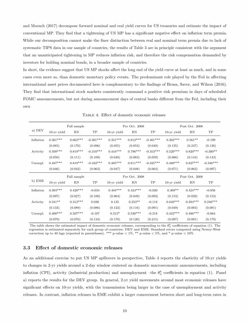
Table 4: Effect of domestic economic releases

a) DEV

Full sample Pre Oct. 2008 Post Oct. 2008

10-yr yield RN TP 10-yr yield RN TP 10-yr yield RN TP

Inflation 0.361*** 0.662*** -0.301*** 0.351*** 0.812*** -0.461*** 0.362*** 0.561** -0.199

(0.085) (0.170) (0.096) (0.055) (0.053) (0.049) (0.135) (0.247) (0.126)

Activity 0.509*** 0.819*** -0.310*** 0.444*** 0.796*** -0.353*** 0.520*** 0.820*** -0.300**

(0.050) (0.111) (0.109) (0.048) (0.063) (0.059) (0.066) (0.144) (0.143)

Unempl. 0.487*** 0.819*** -0.332*** 0.485*** 0.811*** -0.325*** 0.480*** 0.827*** -0.346***

(0.046) (0.042) (0.063) (0.047) (0.048) (0.064) (0.071) (0.063) (0.097)

b) EME

Full sample Pre Oct. 2008 Post Oct. 2008

10-yr yield RN TP 10-yr yield RN TP 10-yr yield RN TP

Inflation 0.394*** 0.428*** -0.034 0.404*** 0.424*** -0.020 0.369** 0.424*** -0.056

(0.097) (0.027) (0.100) (0.064) (0.049) (0.092) (0.153) (0.029) (0.153)

Activity 0.341** 0.312*** 0.030 0.135 0.253** -0.118 0.640*** 0.394*** 0.246***

(0.133) (0.089) (0.086) (0.122) (0.116) (0.091) (0.049) (0.083) (0.081)

Unempl. 0.400*** 0.507*** -0.107 0.312* 0.530*** -0.218 0.422*** 0.486*** -0.064

(0.079) (0.076) (0.134) (0.170) (0.120) (0.215) (0.097) (0.091) (0.179)

The table shows the estimated impact of domestic economic releases, corresponding to the θhn coefficients of equation (1). Theregression is estimated separately for each group of countries: DEV and EME. Standard errors computed using Newey-Westcorrection up to 40 lags (reported in parentheses). *** p-value < 1%, ** p-value < 5%, and * p-value < 10%.

3.3 Effect of domestic economic releases

As an additional exercise to put US MP spillovers in perspective, Table 4 reports the elasticity of 10-yr yields

to changes in 2-yr yields around a 2-day window centered on domestic macroeconomic announcements, including

inflation (CPI), activity (industrial production) and unemployment –the θhn coefficients in equation (1). Panel

a) reports the results for the DEV group. In general, 2-yr yield movements around most economic releases have

significant effects on 10-yr yields, with the transmission being larger in the case of unemployment and activity

releases. In contrast, inflation releases in EME exhibit a larger comovement between short and long-term rates in

10

the earlier sample, a pattern which is reversed in favor of activity and unemployment post October 2008.

All in all, the magnitudes of the effects are comparable to the impact of US MP on long-term yields, although their

composition is different. As was the case for domestic MP events, we see a strong positive impact on RN rates,

partly offset by a negative movement in TP.

4 Interpreting US MP spillover channels

Table 2 documents that, while the effects of US MP shocks to overall long-term yields is quantitatively similar across

DEV and EME groups, the composition of yield changes differ, suggesting in principle different underlying spillover

mechanisms. This section explores alternative explanations to account for these patterns.12

Two main hypotheses are generally mentioned as possible explanations for the comovement between US MP and

international yields. According to the first, yield comovement during FOMC meetings could reflect an adjustment

of financial markets to the revelation of US macroeconomic conditions, potentially correlated with those of other

countries. Under this information channel, the reaction of foreign yields anticipates MP moves in these countries due

to commonality in underlying conditions, and should therefore not be interpreted as a spillover in the causal sense.

A second mechanism, which we refer to as the exchange rate channel, points to a more causal effect of US MP on the

decision of other central banks. Under this mechanism, MP abroad might partially follow the Fed to avoid currency

movements arising from interest rate differentials. Such response could be motivated by inflationary pressures

from exchange rate pass-through and/or trade balance considerations. Sections 4.1 and 4.2 investigate these two

hypotheses and provide additional evidence to establish their relative merits as possible explanations behind our

results. Section 4.3 discusses the connection of our results with the broader international finance literature.

4.1 The information channel

Economic fundamentals –inflation, activity and/or unemployment– may be correlated between the US and other

countries. If, in addition, FOMC meeting are times where information about US fundamentals is revealed to the

markets, then one could expect MP rates in other countries to be correlated with Fed decisions. If this mechanism,

which we refer to as the information channel, dominates the international transmission of US MP documented

above, then such transmission should not be regarded as a spillover in the causal sense, but merely as comovement

reflecting common underlying economic trends. To investigate the relevance of this channel, one must document i)

whether there is a significant degree of comovement between US and other countries’ fundamentals, and ii) whether

information about US fundamentals is indeed revealed at FOMC meetings.

The first condition has found support in the evidence. For much of the post financial crisis period, the US and other

advanced economies –in particular the Eurozone, Japan, and the UK– displayed similar patterns of persistently low

inflation and activity. More formally, Jotikasthira, Le, and Lundblad (2015) document that the observed comovement

between yield curves in the US and other advanced countries’ (Germany and the UK) depend on common underlying

12There is little evidence in the current literature to help narrow down the potential mechanisms behind the international transmissionof interest rates. Bauer and Neely (2014) study the effects on foreign yields of LSAP’s in the US, including a small sample of advancedeconomies and distinguishing between RN rates (which they dub the signaling channel), and TP. However, they do not investigate theeconomic mechanisms underlying their results.

11

factors. Specifically, interest rates depend on a set of macro variables, and those variables in Germany and the UK

depend on both a global factor as well as a US factor, particularly so for inflation.

More problematic is to find support for the second condition –the revelation of fundamentals during FOMC meetings–,

since we have chosen the event study around FOMC days precisely because these are days in which the main event is

the meeting itself, having zero overlap with US economic releases and minimal overlap with events in other countries

(see Table 11, B). It is not obvious therefore how an informational mechanism would play out within our particular

identification strategy. One possibility is that the market learns something about the state of the economy from the

FOMC minutes that could not be anticipated from the processing of publicly available economic releases accumulated

up to that point. This interpretation relies on some form of superior analysis or insight in the way the Fed processes

commonly known information.

Several papers have formally studied whether Fed forecasts of macroeconomic variables can beat the market in a

consistent fashion. While there is some evidence of forecasting superiority by the Fed in older studies, more recent

papers document a narrowing of this advantage post 2000.13 One could still argue the FOMC minutes may provide

relevant signals (in the Bayesian sense) that are incorporated in market expectations as long as they have some

forecasting power –whether or not it beats market forecasts. We now present two pieces of evidence that tend to

downplay the role of this particular channel.

The first evidence is based on comparing the elasticity of international yields to US short-term rates in days of

FOMC announcement compared to other days. Hanson and Stein (2015) argue that non-FOMC days should have a

comparably higher share of macro news, vis-a-vis Fed’ s reaction-function news (what the Fed will do about the

macro news in terms of policy). Conversely, while FOMC days could still reveal macro information, they should have

a relatively larger share of reaction-function news. Therefore, if the elasticity of long-term rates to short-term rate

movements around FOMC days is driven by macro news, this elasticity should be even stronger during non-FOMC

days. They find the opposite.

Based on a similar idea, we calculate the elasticity of long-term rates abroad to changes in US 2-yr yields around

specific US macroeconomic release dates, including inflation (CPI), activity (IP), and unemployment announcements

–the δhn coefficients in equation (1). Notice that this is an even starker comparison than the one documented by

Hanson and Stein (2015), since we select specific US macroeconomic release dates as a benchmark for comparing the

elasticities with respect to FOMC days, whereas they use all non-FOMC days as control. Table 5 shows the results.

For DEV, all US macroeconomic release dates show a significant comovement between US 2-yr and foreign 10-yr

yields (with the bulk of the effects acting through the RN component), but the point estimates are all below the

corresponding effects of US MP shocks reported in Table 2. In fact, difference tests reveal that the transmission of

US short-term rates to DEV long-term yields is in general significantly larger during FOMC meetings than during US

macroeconomic releases. The only exceptions are unemployment releases in the first half of the sample, and activity

in the second part of the sample, where the larger coefficient associated with US MP shocks is not statistically

significant at 5% confidence levels.

13Romer and Romer (2000) document superior performance of Fed forecasts pre 1991, while Gavin and Mandal (2003), and Gamberand Smith (2009), find a deterioration in forecasting advantage when extending the sample up to the early 2000’s. Similarly, D’ Agostinoand Whelan (2008) find that extending the sample leads to forecasting superiority by the Fed only on very short-term (within thequarter) projections of inflation, but not on other macroeconomic variables or forecast horizons.

12

Table 5: Response of 10-yr yields during US economic releases

a) DEV

Full sample Pre Oct. 2008 Post Oct. 2008

10-yr yield RN TP 10-yr yield RN TP 10-yr yield RN TP

US Inflation 0.186*** 0.129*** 0.057 0.209*** 0.173*** 0.036 0.101** 0.031 0.069

(0.028) (0.035) (0.036) (0.033) (0.044) (0.044) (0.049) (0.050) (0.054)

US Activity 0.227*** 0.257*** -0.030 0.179*** 0.231*** -0.052 0.335*** 0.313*** 0.022

(0.024) (0.036) (0.038) (0.027) (0.042) (0.039) (0.060) (0.069) (0.093)

US Unempl. 0.305*** 0.361*** -0.056*** 0.307*** 0.376*** -0.069*** 0.307*** 0.320*** -0.012

(0.015) (0.021) (0.022) (0.018) (0.026) (0.027) (0.026) (0.036) (0.033)

b) EME

Full sample Pre Oct. 2008 Post Oct. 2008

10-yr yield RN TP 10-yr yield RN TP 10-yr yield RN TP

US Inflation -0.055 -0.011 -0.044 -0.027 -0.036 0.009 -0.174* 0.055 -0.230*

(0.063) (0.037) (0.073) (0.075) (0.047) (0.086) (0.105) (0.056) (0.132)

US Activity 0.037 0.038 -0.001 0.006 0.056 -0.050 0.022 -0.045 0.067

(0.054) (0.049) (0.064) (0.064) (0.062) (0.078) (0.100) (0.063) (0.104)

US Unempl. 0.051* 0.036* 0.015 0.042 0.046* -0.004 0.085** 0.023 0.062

(0.031) (0.021) (0.038) (0.040) (0.027) (0.049) (0.040) (0.029) (0.050)

The table shows the impact of US economic releases, corresponding to the δhn coefficients of equation (1). The regression isestimated separately for each group of countries: DEV and EME. Standard errors computed using Newey-West correction up to40 lags (reported in parentheses). *** p-value < 1%, ** p-value < 5%, and * p-value < 10%.

For EME countries, the effect of changes in the US 2-yr treasury around macroeconomic releases is generally not

significant, with a few exceptions where small effects are found. Not surprisingly, we find that the impact of US MP

on foreign bond yields is significantly higher than the corresponding effect of US macroeconomic releases.

This evidence is thus not supportive of the informational channel. Following the argument in Hanson and Stein

(2015), the fact that international yields comove less with US interest rates during US economic releases (days with

a larger share of US macro news) than during FOMC meetings suggests that the main driving force between such

comovement must be unrelated to the revelation of US macroeconomic fundamentals.

The second piece of evidence we present is based on testing directly whether yield changes during FOMC meetings

affect macroeconomic variables in other countries.14 Here it is important to recognize that, beyond a signaling

channel of future macroeconomic conditions, US yield changes may also affect macroeconomic conditions in a causal

manner through tighter policy. But notice that these channels are, a priori, associated with opposite signs: while the

signaling channel suggests a positive correlation between US yield changes and future macro conditions (i.e., the Fed

is tightening policy because it anticipates better macro performance in the US, in turn correlated with activity and

inflation abroad), the causal effect predicts a negative relation –a tighter Fed policy, all else equal, is contractionary

for other economies, as has been widely documented.15

To test this hypothesis we need to adjust to a monthly-frequency empirical strategy to fit in the frequency of

macroeconomic releases. We compute the monthly change in the 2-yr US yield and separate it into two components:

the change around the FOMC meeting of that respective month (the same measure of US MP shock as above), and

the difference between the total change in the rate during the month and the FOMC component. The idea is that

14We thank the referee for suggesting this test.15See Kim (2001), and Canova (2005), among others.

13

the first component captures the surprise component in Fed policy during the month, while the second component

incorporates all other information that affected interest rates during the month.16 That is, at each month t where

there is an FOMC meeting, we have ∆US 2Y Rt = FOMCt + Restt. We then regress different leads of activity

and inflation in the countries included in each of our DEV and EME samples using monthly panel regressions.

Specifically, we estimate the following model:

xj,t+h = α+ β1 ∗ FOMCt + β2 ∗Restt + γ ∗ xj,t + εj,t+h, (5)

where xj,t+h correspond to annual growth rates of realized macroeconomic variables at horizon t+h for each country

j (activity and inflation, depending on the regression). Table 6 summarizes the results. We find that increases in

US 2-yr rates have a negative effect on future activity and inflation abroad, for both components of the overall

change in yields. This suggests that the impact of higher US interest rates on foreign activity and inflation work

predominantly through the standard channel –a higher interest rates in the US is contractionary for other countries,

consistent with the literature on the international real spillovers of US MP.

Altogether, the evidence presented in this section suggests that, while impossible to completely rule out, the

informational channel is unlikely to be the main driver behind the observed comovement between US 2-yr yields and

international bond yields at longer maturities. We remark again that the evidence presented here should not be

interpreted as against commonality in economic fundamentals between the US and other economies –well documented

in other studies–, but merely against the interpretation that FOMC meetings are episodes where significant news

about such fundamentals are revealed to the markets.

4.2 The exchange rate channel

By affecting the relative yield of dollar-denominated instruments, US MP drives changes in portfolio positions

between US and international assets. In particular, an expansionary US MP shock will, for a given exchange rate,

increase the demand for foreign bonds. Within the standard Mundell-Fleming paradigm, the equilibrium response in

foreign yields and exchange rates will depend, in turn, on the reaction of foreign central banks. The more other

central banks follow the Fed, the narrower the resulting yield differential and the more contained the appreciation of

their currencies. We will refer to the effects of US MP shocks on foreign yields that result from this mechanism as

the exchange rate channel.

As the evidence in section 3 suggests however, the adjustment not only takes place through changes in expected

foreign MP (the RN channel), as there are relevant movements in bond term premia. Indeed, several recent papers

have emphasized the “risk-taking” channel of US MP. According to this mechanism, an expansionary stance of US

MP drives a search for yields in other assets, including longer-maturity US treasuries and higher risk securities

(corporate bonds, MBS products), as well as foreign assets.17 The addition of term premia as a margin of adjustment

makes the underlying transmission mechanisms less straightforward than in the standard Mundell-Fleming model.

16A related approach is followed by Bernanke and Kuttner (2005), who study the dynamic effects of the surprise component of FFRchanges on equity returns using a VAR approach at monthly frequency (see section II of their paper).

17See Hanson and Stein (2015), Krishnamurthy and Vissing-Jorgensen (2011), Bruno and Shin (2015), and Rey (2015). The risksbeing taken through larger international positions include currency risk (Gabaix and Maggiori, 2015) as well as default risk in the case ofemerging countries.

14

Table 6: Response of international macroeconomic variables to US monetary policy

a) DEV

Inflation Activity

Pre Oct. 2008 Post Oct. 2008 Pre Oct. 2008 Post Oct. 2008

h FOMC Rest FOMC Rest FOMC Rest FOMC Rest

1 -0.367** 0.236*** -0.046 0.100 -3.004** 0.219 3.353 -1.999

2 -0.062 0.170** -0.083 0.350** -2.274 1.349*** -2.901 0.465

3 0.094 0.083 -0.158 0.273 -5.219*** -0.505 0.603 1.830

4 -0.026 -0.107 -1.099 0.281 -3.682** 1.913*** 0.455 0.145

5 -0.106 -0.192** -0.453 0.209 -5.684*** 0.301 0.096 1.867

6 -0.460** -0.305*** -0.311 0.202 -4.750*** -0.654 8.753 3.771

7 -1.141*** -0.391*** -0.753 0.158 -4.988*** -0.223 1.181 -1.040

8 -2.143*** -0.427*** -0.538*** 0.221 -4.967** -2.338*** 4.017 1.526

9 -1.649*** -0.252*** -0.440** 0.135 -5.171*** -1.904*** 6.281 4.161

10 -0.516* -0.078 -1.288** 0.283* -3.677** -1.151 1.643 2.021

11 0.140 -0.105 -1.290* 0.139 -1.407 -0.977* -4.176 3.514*

12 -0.082 -0.031 -1.381* -0.039 1.932 -0.041 -6.630 -1.564

b) EME

Inflation Activity

Pre Oct. 2008 Post Oct. 2008 Pre Oct. 2008 Post Oct. 2008

h FOMC Rest FOMC Rest FOMC Rest FOMC Rest

1 -0.066 0.338*** 1.031 -0.039 -4.509** 0.155 -14.099*** -2.041

2 -0.035 0.375*** 1.629 0.782*** -2.249 2.384*** -7.534 -4.115***

3 -0.191 0.385** 1.063 0.757** -6.189*** -0.911 -6.714* -0.785

4 -0.661 0.126 1.074 0.519 -3.746** 2.061*** -14.261*** -3.400**

5 -1.256*** -0.124 1.091 0.605 -7.087*** 0.458 -14.949*** -3.970***

6 -1.533*** -0.309 0.941 0.686 -0.076 -1.110* -0.209 -0.815

7 -1.555*** -0.413* 0.132 0.148 -4.683** -0.567 4.840 -1.473

8 -2.003*** -0.398* 0.989 0.397 -3.023 -3.129*** -2.076 -0.503

9 -2.209*** -0.357* -0.037 0.466 -6.318*** -1.464** -0.212 -1.357

10 -1.485** -0.234 -2.900* -0.042 -1.867 -0.813 12.929*** -0.817

11 -0.363 -0.004 -1.873 -0.108 2.743 0.043 -3.996 2.279**

12 -0.397 -0.021 -2.329 -0.194 7.329*** 1.268* 3.340 0.235

The table reports the impact of changes in the components of the US 2-yr rates defined in equation (??) for a givenmonth (in bp), in effective inflation and activity data h-months ahead (also in bp) –the β1 and β2 coefficients inequation (5). Standard errors computed using Newey-West correction up to 40 lags (reported in parentheses). ***p-value < 1%, ** p-value < 5%, and * p-value < 10%.

15

In particular, it is not obvious whether the relevant interest rate differential behind exchange rate pressures are

expected MP rates (the RN component) or overall yields, nor why the reaction in yields components differs across

country groups.

To provide a coherent interpretation of the exchange rate channel in the context of our previous results, A presents

a model about the international transmission of US MP that extends the framework developed in Blanchard, Adler,

and Carvalho Filho (2015). In that paper, imperfect substitutability between international assets drives capital

flows across countries in response to interest rate differentials. Their analysis stresses how two main tools used

by central banks to confront flows –standard MP and (sterilized) exchange rate interventions (FXI henceforth)–

have different effects on interest rates, exchange rates, and the resulting capital inflows in equilibrium. To illustrate,

consider the case of a capital inflow into country-j (for example, as a response to an expansionary US MP shock).

If the central bank remains inactive, capital inflows that respond to interest differentials will be large, and so

will be the appreciation of the domestic currency. In contrast, a MP response that narrows the interest rate

differential would contain inflows and exchange rate pressures. Yet the central bank could confront the same situation

through direct FXI (buying USD in this case), and may in principle control both exchange rate and short-term

interest rate movements –to the extent that sterilized interventions have meaningful effects on the exchange rate.

However, the authors show that such policy response will increase the resulting capital inflows in equilibrium, as the

market stabilization mechanism that would normally act through a currency appreciation (and the ensuing expected

depreciation) is inhibited by the intervention.

Our model extends this framework by including a long-term bond market in each country. This allows us to study

the effects of US MP shocks on interest rates at longer maturities, as well as their RN and TP components. In

the US bond market, long-term yields are connected to short-term policy rates both through RN rates and term

premia, where this last term is influenced by a risk-taking factor. This risk-taking factor is in turn a negative

function of US MP. The model assumes that overall capital inflows to other countries depend endogenously on

interest rate differentials against the US in both short and long-term bonds. In particular, there are foreign investors

in the long-term bond market whose demand is a positive function of yield differentials against the US, net of the

expected depreciation of the domestic currency. Implicit in this assumption is the notion that US and international

assets are imperfect substitutes, and that lower yields in US bonds incentivize larger risk-taking in foreign bonds.

Also, MP in the receiving country responds to the exchange rate (i.e., is reduced following a currency appreciation

against the USD), which can be rationalized from inflationary pressures (exchange rate pass-through) or trade

balance concerns. In addition, the central bank may choose to intervene the FX market by buying/selling USD

against capital inflows/outflows. The equilibrium of the model is pinned down by a balance of payments equilibrium

condition in which capital inflows net of FXI must finance the trade balance deficit. In the equilibrium, the main

objects of interest in the model are linear functions of US MP shocks.

We now briefly summarize the main results of the model, their implications for interpreting the evidence presented

in Section 3, and the additional testable predictions they deliver (which we test below). Following a negative US MP

shock that increases the global risk-taking factor, capital flows into the US and country-j’s long-term bond markets.

The equilibrium level of capital inflows is a function of country-j’s prevailing interest rate differentials in both short-

and long-term securities. The effect on the main endogenous variables depends, in turn, on the reaction of policy

16

in the receiving country, as summarized in propositions 1 and 2 in the model of A, which we reproduce here for

convenience.

Proposition 1: In reaction to an expansionary US MP shock, a higher sensibility of domestic MP to exchange rate

fluctuations in country-j will imply a) a weaker appreciation of the currency against the USD; b) a weaker response

of capital inflows; c) a stronger effect in the RN component of long-term yields, and d) an ambiguous effect in the

TP component of long-term yields.

The intuition for these results is as follows. In response to a more expansionary US MP, a central bank that

reacts more to the ensuing appreciation of the currency by changing its own MP will tend to narrow interest rate

differentials. This will contain capital inflows (part b) and reduce the resulting appreciation of the currency (part a).

The effects on the long-term bond market are less obvious, however. Because foreign investors in the domestic bond

market trade off positive interest rate differentials against an expected depreciation of the domestic currency going

forward, the equilibrium response in long-term yields will be larger whenever the initial appreciation is contained by

the action of domestic MP. Hence, overall yields fall by more. On the other hand, a stronger reaction of domestic

MP mechanically implies a larger response of expected MP into the future, implying a larger elasticity of the RN

component of long-term yields (part c). The effect on the TP component, which is the difference between yields and

the RN component, is therefore ambiguous (part d).

Proposition 2: In reaction to an expansionary US MP shock, a higher degree of central bank FXI in country-j

will imply a) a weaker appreciation of the currency against the USD; b) a stronger response of capital inflows; c) a

weaker effect on the RN component of long-term yields, and d) a stronger effect in the TP component.

To understand this prediction, notice that if central banks intervene more, any given level of capital inflows will

have a weaker effect on the domestic currency (part a). Since a currency appreciation (and the ensuing expected

depreciation) in response to foreign inflows is a market force that tends to deter such flows, FXI strengthen flows

precisely by dampening the corrective response played by exchange rates (part b). At the same time, a weaker

impact on the exchange rate implies a more muted response of the standard MP tool (for a given value of the MP

response parameter), reducing the sensitivity of the RN component (part c). But this implies that the adjustment in

domestic long-term yields, which drop even more under FXI due to the surge in capital inflows, must be made to a

larger extent by a compression of the TP component (part d).

The evidence presented in Section 3 documents only the reaction of yields and their components to US MP shocks,

and thus allows at least two different interpretations in the context of the model. First, according to proposition

1, the relatively weak response of RN rates in EME might reflect a lower sensitivity of domestic MP to currency

movements in these countries relative to DEV. However, such policy reaction would imply a stronger response of

exchange rates to US MP shocks in EME. The alternative hypothesis is that central banks in EME are more prone

to use FXI. According to proposition 2, this would also explain a weaker response of RN rates, but now as a result

of lower effective currency movements and not from a lower sensitivity of domestic MP to exchange rate fluctuations.

In addition, such response would amplify the response of capital inflows to EMEs, generating unambiguously larger

movements in long-term yields concentrated in the TP component.

A priori, the predictions from proposition 2 seem to square better with the empirical evidence. Indeed, central bank

interventions in FX markets have been widely documented for emerging economies, where managed floats are much

17

more common than in developed countries. Table 12 in B includes a survey of the available evidence about FX

intervention activity for all the countries in our sample, confirming this view. Moreover, recent literature shows that,

once endogeneity issues are properly addressed (using high frequency intra-day data), interventions appear to be

an effective exchange rate stabilizing tool, at least in the short term.18 This prediction is also consistent with the

evidence reported in Section 3, which shows a stronger response to US MP shocks in the TP component of yields for

EME relative to DEV.

To further distinguish between these predictions, we now provide evidence of the two additional endogenous variables

not addressed thus far, namely the reaction of exchange rates and capital flows around US MP events. Table 7

shows the impact of US MP shocks on exchange rates. The results are from a regression that replaces the interest

rate variables of the left-hand-side of equation (1) with the cumulative NER response for each country over the

same interval around the FOMC meeting. The NER is in units of foreign currency per USD, so an increase is a

depreciation against the dollar. We find highly statistically significant effects of US MP shocks on exchange rates for

the DEV sample. Specifically, a 10 bp US MP shock would depreciate the exchange rate in the DEV sample by

about 75 bp in the full sample, an effect that has increased from 55 bp in the first half to 109 bp in the period post

October 2008. For EME, we also find statistically significant effects, although of smaller magnitude. The full sample

coefficient is just 33 bp, increasing from 16 to 66 bp when comparing both sub-periods. In short, exchange rates

react in the anticipated direction in both groups of countries, although the effect is roughly half as large for EME. 19

Table 7: US monetary policy and exchange rates

Full sample Pre Nov. 2008 Post Nov. 2008

DEV 7.50*** 5.47*** 10.92***

(0.45) (0.39) (0.83)

EME 3.52*** 1.93*** 6.66**

(0.44) (0.49) (0.77)

The table reports the impact of a 1 bp change in the US2-yr rate on nominal exchange rate changes during the MPevent window. The exhange rate is defined as units of thedomestic currency per USD (an increase is a depreciationagainst the dollar). The coefficients are in bp. Standarderrors computed using Newey-West correction up to 40 lags(reported in parentheses). *** p-value < 1%, ** p-value< 5%, and * p-value < 10%.

One possible concern with this empirical strategy is that exchange rates could anticipate MP shocks. Previous

research has pointed out that FFR futures tend to correctly anticipate most of Fed policy changes (Cochrane and

Piazzesi, 2002). A recent paper by Karnaukh (2016) documents that, while the anticipation in FFR futures happen

several days in advance, the exchange rate reacts only about 2 days prior to the actual change (when the Fed tightens

policy, the USD appreciates, and vice-versa). If exchange rates react in anticipation of our MP events, our 2-day

18In fact, all but three countries in the DEV sample follow clean floating regimes, and within these exceptions, both the CzeckRepublic and Switzerland have used the euro as a reference currency, making them clean floaters against the USD. For further evidenceabout FXI activity and its effectiveness in emerging markets see Sarno and Taylor (2001), Levy-Yeyati and Sturzenegger (2003), Husain,Mody, and Rogoff (2005), Menkhoff (2010), Ghosh, Ostry, and Chamon (2016), and Fratzscher, Gloede, Menkhoff, Sarno, and Stohr(2017).

19Evidence of weaker exchange rate effects in emerging countries is also found in a recent paper by Hausman and Wongswan (2011),which use an event study methodology similar to ours but for an earlier time period. They find that, generally, the USD depreciatesfollowing a US MP easing, but significantly so only against developed currencies.

18

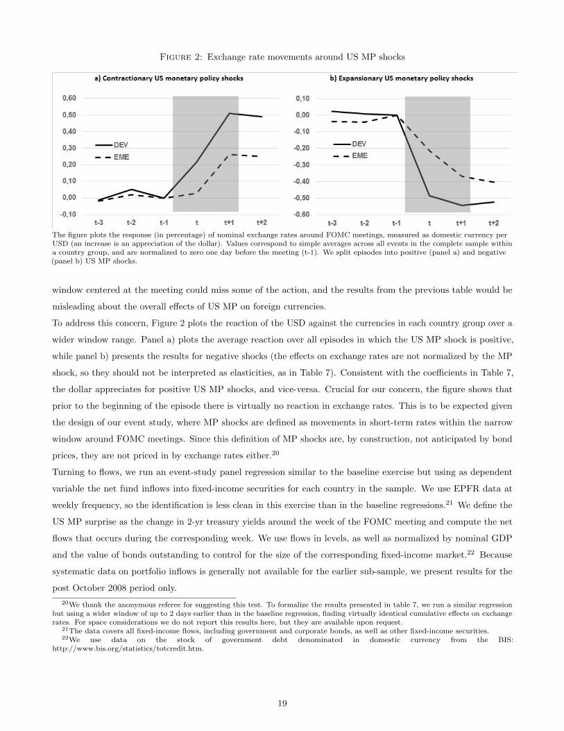
Figure 2: Exchange rate movements around US MP shocks

The figure plots the response (in percentage) of nominal exchange rates around FOMC meetings, measured as domestic currency perUSD (an increase is an appreciation of the dollar). Values correspond to simple averages across all events in the complete sample withina country group, and are normalized to zero one day before the meeting (t-1). We split episodes into positive (panel a) and negative(panel b) US MP shocks.

window centered at the meeting could miss some of the action, and the results from the previous table would be

misleading about the overall effects of US MP on foreign currencies.

To address this concern, Figure 2 plots the reaction of the USD against the currencies in each country group over a

wider window range. Panel a) plots the average reaction over all episodes in which the US MP shock is positive,

while panel b) presents the results for negative shocks (the effects on exchange rates are not normalized by the MP

shock, so they should not be interpreted as elasticities, as in Table 7). Consistent with the coefficients in Table 7,

the dollar appreciates for positive US MP shocks, and vice-versa. Crucial for our concern, the figure shows that

prior to the beginning of the episode there is virtually no reaction in exchange rates. This is to be expected given

the design of our event study, where MP shocks are defined as movements in short-term rates within the narrow

window around FOMC meetings. Since this definition of MP shocks are, by construction, not anticipated by bond

prices, they are not priced in by exchange rates either.20

Turning to flows, we run an event-study panel regression similar to the baseline exercise but using as dependent

variable the net fund inflows into fixed-income securities for each country in the sample. We use EPFR data at

weekly frequency, so the identification is less clean in this exercise than in the baseline regressions.21 We define the

US MP surprise as the change in 2-yr treasury yields around the week of the FOMC meeting and compute the net

flows that occurs during the corresponding week. We use flows in levels, as well as normalized by nominal GDP

and the value of bonds outstanding to control for the size of the corresponding fixed-income market.22 Because

systematic data on portfolio inflows is generally not available for the earlier sub-sample, we present results for the

post October 2008 period only.

20We thank the anonymous referee for suggesting this test. To formalize the results presented in table 7, we run a similar regressionbut using a wider window of up to 2 days earlier than in the baseline regression, finding virtually identical cumulative effects on exchangerates. For space considerations we do not report this results here, but they are available upon request.

21The data covers all fixed-income flows, including government and corporate bonds, as well as other fixed-income securities.22We use data on the stock of government debt denominated in domestic currency from the BIS:

http://www.bis.org/statistics/totcredit.htm.

19

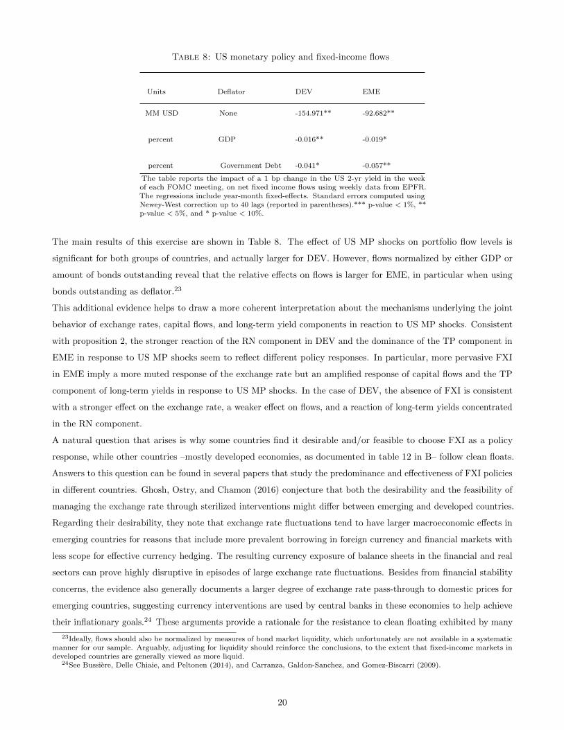
Table 8: US monetary policy and fixed-income flows

Units Deflator DEV EME

MM USD None -154.971** -92.682**

percent GDP -0.016** -0.019*

percent Government Debt -0.041* -0.057**

The table reports the impact of a 1 bp change in the US 2-yr yield in the weekof each FOMC meeting, on net fixed income flows using weekly data from EPFR.The regressions include year-month fixed-effects. Standard errors computed usingNewey-West correction up to 40 lags (reported in parentheses).*** p-value < 1%, **p-value < 5%, and * p-value < 10%.

The main results of this exercise are shown in Table 8. The effect of US MP shocks on portfolio flow levels is

significant for both groups of countries, and actually larger for DEV. However, flows normalized by either GDP or

amount of bonds outstanding reveal that the relative effects on flows is larger for EME, in particular when using

bonds outstanding as deflator.23

This additional evidence helps to draw a more coherent interpretation about the mechanisms underlying the joint

behavior of exchange rates, capital flows, and long-term yield components in reaction to US MP shocks. Consistent

with proposition 2, the stronger reaction of the RN component in DEV and the dominance of the TP component in

EME in response to US MP shocks seem to reflect different policy responses. In particular, more pervasive FXI

in EME imply a more muted response of the exchange rate but an amplified response of capital flows and the TP

component of long-term yields in response to US MP shocks. In the case of DEV, the absence of FXI is consistent

with a stronger effect on the exchange rate, a weaker effect on flows, and a reaction of long-term yields concentrated

in the RN component.

A natural question that arises is why some countries find it desirable and/or feasible to choose FXI as a policy

response, while other countries –mostly developed economies, as documented in table 12 in B– follow clean floats.

Answers to this question can be found in several papers that study the predominance and effectiveness of FXI policies

in different countries. Ghosh, Ostry, and Chamon (2016) conjecture that both the desirability and the feasibility of

managing the exchange rate through sterilized interventions might differ between emerging and developed countries.

Regarding their desirability, they note that exchange rate fluctuations tend to have larger macroeconomic effects in

emerging countries for reasons that include more prevalent borrowing in foreign currency and financial markets with

less scope for effective currency hedging. The resulting currency exposure of balance sheets in the financial and real

sectors can prove highly disruptive in episodes of large exchange rate fluctuations. Besides from financial stability

concerns, the evidence also generally documents a larger degree of exchange rate pass-through to domestic prices for

emerging countries, suggesting currency interventions are used by central banks in these economies to help achieve

their inflationary goals.24 These arguments provide a rationale for the resistance to clean floating exhibited by many

23Ideally, flows should also be normalized by measures of bond market liquidity, which unfortunately are not available in a systematicmanner for our sample. Arguably, adjusting for liquidity should reinforce the conclusions, to the extent that fixed-income markets indeveloped countries are generally viewed as more liquid.

24See Bussiere, Delle Chiaie, and Peltonen (2014), and Carranza, Galdon-Sanchez, and Gomez-Biscarri (2009).

20

EMEs, explaining why they might be inclined to seek both MP independence and exchange rate stability through

sterilized FXI.

With respect to its feasibility, Ghosh, Ostry, and Chamon (2016) argue that the size of central banks’ foreign

reserves, relative to normal currency transaction volumes, is typically much larger in emerging economies. This

suggest that, using a relatively small fraction of their balance sheets, central banks in these countries can have a

meaningful impact in the value of their currencies through direct FX interventions. For developed economies, in

contrast, cross-border flows are likely to respond much more strongly to interest rate differentials against the US

given the closer degree of asset substitutability. This implies that the size of interventions needed to make even a

minor dent on the exchange rate may simply be too large to make it a viable option. This argument also features

prominently in earlier papers such as Rogoff (1984) and Dominguez (1990), among others.

4.3 Discussion

We now relate our findings with two important strands of literature in international finance. The first is the relation

with the Mundell-Fleming paradigm as a benchmark to understand the effects of changes in international interest

rates on domestic nominal and real variables in the presence of imperfect capital mobility. We briefly highlight the

main differences between the predictions of that model and our framework regarding the effects of policy choices by

central banks in dealing with international MP shocks. The second is the literature documenting the failure of the

UIP condition –the so called forward discount puzzle. We briefly review some of its main findings, emphasizing the

consistency with our results and the implications for the spillover mechanisms in our model.

In its simplest form, the Mundell-Fleming model with imperfect capital mobility predicts that a contractionary MP

shock in core economies will affect nominal and real variables in a particular country depending on the reaction of

its monetary authority. If the domestic central bank moves the MP rate one-to-one, the model predicts a complete

stabilization of the exchange rate, but at a rather high cost to domestic output. In contrast, a central bank that

keeps the domestic interest rate constant, and absent any form of FX intervention, will induce a pressure on capital

outflows that will depreciate the domestic currency. In equilibrium, this improves the trade surplus. Flexible

exchange rates hence play a role in cushioning part the negative effect of higher foreign interest rates by enhancing

external demand. While the model in A does not include aggregate demand, its predictions on exchange rates align

well with the standard framework in this case –the flexible exchange rate case– suggesting they would play a similar

absorption role in a general equilibrium framework with endogenous output. Naturally, since our model includes

a long-term bond market and allows for adjustment in term premia, it will deliver somewhat richer predictions

regarding the effect of different MP actions at different segments of the yield curve. In its core predictions however,

the general message regarding the tradeoffs involved in setting interest rates in response to MP spillovers abroad

would not markedly differ from the standard model.

Where our model does departs from this framework is regarding the implications of FXI policies. If the domestic

Central Bank wants to keep MP unchanged and at the same time limit the exchange rate adjustment through

FXI, it must fully compensate for the capital outflow consistent with a lower interest rate differential. Since in the

standard model aggregate demand depends only on short-term interest rates and exchange rates, this combination

of policies would appear to be effective in stabilizing both nominal and real variables. In our model, the inclusion of

21

a long-term bond market opens an additional channel that breaks this result. As discussed above (prediction 2 in

section 4.2), while FXI can achieve both a stabilization of the MP rate and the exchange rate, they cannot control

long-term yields. Our model highlights that stabilizing the currency through FXI will indeed amplify the effect of

yield differentials on capital flows, thus enhancing the endogenous response of term premia. To the extent that

aggregate demand depends on the whole structure of interest rates, this policy reaction will not be able to isolate

the real economy from the external shock. This is the key mechanism that arises in our model which is absent from

the Mundell-Fleming paradigm. We believe this additional mechanism should be added an important consideration

when evaluating the pros and cons of FXI policies.

Our results should also be contrasted with the literature documenting the forward discount puzzle, specifically

regarding its implications for the validity of the underlying spillover mechanisms highlighted by our model. A large

number of studies have investigated the dynamic effects of US MP shocks on exchange rates, including Clarida

and Galı (1994), Eichenbaum and Evans (1995), Kim and Roubini (2000), and Scholl and Uhlig (2008), among

others. All these studies focus on advanced countries, and differ in terms of the particular structural identification

strategy chosen within vector autoregression models. Consistent with our results, these papers generally find that an

expansionary US MP shock depreciates the USD, but their different identification strategies translate into varying

results regarding the persistence of exchange rate dynamics –that is, whether the exchange rate exhibits immediate

or delayed overshooting– , and thus into distinct predictions for the forward discount puzzle.

Regarding the implications of this evidence on the spillover mechanism highlighted by our model, it’s important to

stress that as long as an expansionary US MP shock results in an inflow of capital into other countries –and that such

inflow in turn depends on the policy reaction by monetary authorities in that country–, our qualitative predictions

regarding the impact on long-term yields would remain largely unchanged irrespective of whether the depreciation of

the USD is sudden or gradual. This distinction is obviously important for whether or not MP shocks are associated

with the forward discount puzzle, but as long as both scenarios imply a positive inflow into fixed-income markets to

other countries, they both predict a narrowing of term premia abroad, thus explaining the spillover to long-term

yields documented in section 3. In other words, our results do not hinge on whether the UIP condition holds in

the data, but rather in whether fixed-income flows follow the direction of yield differentials in response to US MP

shocks, and whether those flows are in turn affected by FXI.

A related literature focuses on the forward discount puzzle in more detail, but abstracting from the identification of

MP shocks. Bansal and Dahlquist (2000) find evidence of the puzzle for developed economies, but not for their

sample of emerging countries. Lustig, Roussanov, and Verdelhan (2014) show that a positive interest rate differential

against the USD in a basket of advanced economies forecasts positive excess returns of these currencies. They

propose an affine model in which high interest rates differentials against the USD take place when the US economy

is hit by shocks which increase the volatility of the stochastic discount factor (SDF) relevant for US investors. In

equilibrium, US investors require larger compensation for buying foreign bonds in these states of nature, which

explains their higher returns. At face value, these studies do appear to be in tension with the mechanism of our

model, since lower rates in the US are associated with higher, not lower, risk premia in foreign currencies.

The tension between these results and our findings can perhaps be resolved by noticing that a low interest rate

environment in the US and an expansionary US MP surprise may well have different asset pricing implications.

22

In line with the argument in Lustig, Roussanov, and Verdelhan (2014), a low interest rate environment may be

the consequence of a relatively weak US macroeconomy, one in which US investors must be compensated with

higher excess returns in order to invest in foreign instruments. But within this environment, a MP decision and/or

communique by the Fed that is perceived more expansionary than what could be anticipated from economic

fundamentals –the notion of MP shocks captured by our methodology– may well incentivize investors at the margin

to build up larger positions in foreign securities offering higher yields. This is consistent with a USD that depreciates

on impact, in line with our results. The key distinction here is that that macroeconomic fundamentals, by pinning

down the moments of the SDF, drive both interest rates in the US and international risk premia. On the other

hand, shocks to US MP above and beyond fundamentals need not affect the SDF and therefore may well incentivize

flows into foreign securities due to their higher relative yield. It should be stressed that this mechanism is not only

consistent with our model and results, but also with the existing literature studying the “risk taking channel” of US

MP cited above.

Supportive evidence in this regard is also provided in the aforementioned paper by Karnaukh (2016). She documents

that the delayed reaction of the dollar vis-a-vis FFR futures in anticipation of rate changes actually goes “in the

right direction” that is, the dollar depreciates when FFR futures are pricing in a rate cut. Moreover, she finds that

during days when either no FOMC meetings take place, or during those meeting in which the rate is expected to be

maintained, the results align closely with Lustig, Roussanov, and Verdelhan (2014); namely, higher rates against the

USD forecast higher returns of holding foreign currencies – the forward discount puzzle. But in episodes in which

futures are pricing in a change in the FFR, the evidence fails to reject the UIP condition.

While it is beyond the scope of this paper to provide a full-fledged analysis about the conditions under which the

UIP relation is upheld or violated, it is interesting to note that the results of this paper, as well as those from related

event studies focused on US MP shocks, suggests that the logic of interest rate arbitrage seems to square better with

the evidence during days in which significant information about MP is reveled to markets. This interpretation is

reminiscent of the results in Savor and Wilson (2014), who robustly document the success of standard asset pricing

theories, such as the CAPM, during days in which important macroeconomic news are scheduled for announcement.

Further inquiry into this issue seems an important topic for future research.

5 Robustness

We now briefly describe different robustness checks we perform to our baseline econometric specification. For space

considerations, we focus mostly on the coefficients related to US MP spillovers for overall 10-yr yields and their

components. The main tables are included in C.

A first robustness check involves sample selection. To ensure that our main results are not driven by outliers, we

run equation (1) excluding iteratively one country from each group (for example, we run the regressions for DEV

without Japan, then put Japan back in and exclude Sweden, and so forth). These results are reported in Table 13.

The main conclusions remain unaltered, namely, US MP spillover effects are larger in the post October 2008 data,

with similar point estimates for both DEV and EME samples. Moreover, these effects are much more tilted towards

changes in the TP component in the case of EME.

23

The second set of robustness tests include different fixed effects in the panel regression of equation (1), as well as

alternative windows for clustering standard errors (in this case, the differences arise only in the significance of point

estimates). These results are reported in Table 14. For ease of comparison, the third column of the table reproduces

the spillover effects on long-term yields in the baseline regression from Table 2. The point estimates from using

alternative fixed-effects change only marginally. While the significance of the coefficients drop in some specifications,

it is always the case that the impact of US MP shocks on long-term yields is significant at 5% confidence levels, and

its point estimate larger in the post October 2008 period. In the DEV sample, the effect of US MP shocks on RN

rates is always associated with a larger point estimate than the effect on TP, and the significance of the former effect

is always larger than a 5% p-value, while in some specifications the significance on TP falls below the 5% threshold.

For EME, the point estimate on TP is always larger than the effect on the RN component (both significant at 5%

across specifications). Thus, our main conclusions are maintained in these exercises.

A third robustness exercise deals with the methodology for decomposing yields into their RN and TP components.

In Table 15 we reproduce our main regression in Table 2 using the affine term-structure model of Joslin, Singleton,

and Zhu (2011). Its main difference with the methodology of Adrian, Crump, and Moench (2013) is that the prices

of risk associated with the factors driving the yield curve are estimated jointly with the parameters of the VAR

in equation (2) using maximum likelihood.25 Our main quantitative and qualitative results regarding the relative

contribution of yield components for both the DEV and EME samples remain unaltered under this alternative

decomposition methodology.

A fourth robustness check involves using a tighter window for defining the US MP shock. Indeed, the choice of the

appropriate window involves non trivial tradeoffs: while shorter windows help identification by reducing overlap

with other events, they also allow less time for the market to digest the relevant information that may be contained

in FOMC minutes. Table 16 reports the regression results of Table 2, but defining the US MP shock as the change

in the 2-yr US treasury between (the closing of) the day before and the same day of the FOMC meeting (as opposed

to the day after the FOMC statement). Once again, the main qualitative results are maintained, with very minor

differences in the point estimates.

As the final robustness exercise, we use alternative definitions of the interest rate chosen as a measure of US MP

shocks. Table 17 replicates the main regression results of Table 2, but using the change of the 1-yr treasury around

the FOMC meeting, as opposed to the 2-yr treasury used in the baseline specification. In general, the point estimates

are larger, but the qualitative results from the baseline regression remain unaltered. Essentially, the 1-yr and 2-yr

treasury yields have a very strong correlation (0.76 in the complete sample), but the standard deviation of the

former is about 60% of the latter in the post October 2008 period, which explains the larger estimated elasticities

when the 1-yr rate is used. We prefer to use the 2-yr rate in our baseline regressions as it is more likely to capture

the stance of US MP in the medium term. This is especially relevant post October 2008, when changes in the tone of

Fed policy often did not involve revisions in market expectations about the FFR in the coming 12 months.26 Other

25For further discussion of the differences between methodologies, see Section 2.5 of Adrian, Crump, and Moench (2013).26This is particularly the case in some FOMC statements associated with forward guidance. For example, in the FOMC meeting of

Aug. 2011, the press release stated: “The Committee currently anticipates that economic conditions... are likely to warrant exceptionallylow levels for the federal funds rate at least through mid-2013.” At that meeting, the 1-yr rate fell only 3 bp, less than half the effect onthe 2-yr rate. Furthermore, the 2-yr maturity is also used in other related studies, such as Hanson and Stein (2015) and Gilchrist, Yue,and Zakrajsek (2016), which makes results easier to compare.

24

authors have used changes in the short-term FFR futures (typically the next month contract) as an alternative

measure of MP shocks, either directly (as in Bernanke and Kuttner, 2005), or indirectly as instruments (Gertler

and Karadi, 2015). Table 18 contains the results from using 1 year-ahead FFR futures. Alternative 1 defines the

MP shock as the change in the futures around the 2-day window, while Alt. 2 uses the change in futures as an

instrument for the change in the 2-year yield. Results are quantitatively quite similar to the baseline regression.27

6 Conclusions

We document the presence of significant US monetary policy spillovers to domestic bond markets in a sample of

24 countries, including 12 developed and 12 emerging market economies. We rely on an event study methodology

where US monetary policy shocks are identified with the response of short-term US treasury yields within a narrow

window of FOMC meetings, and trace its consequences on international bond yields using panel regressions. We

decompose yields for each individual country into a risk- neutral component, which captures the expected evolution

of short-term rates, and bond term premia, in order to better understand the channels underlying such transmission.

We find that US MP spillovers are statistically and economically significant for both developed and emerging market

economies, and have become relatively larger after the global financial crisis. These spillovers are comparable in

magnitude with the impact of other economic events that move international yield curves, including domestic

monetary policy shocks and economic releases in each country.

While the size of spillovers is comparable across country groups, our results suggest they operate though different

mechanisms, being concentrated in the risk-neutral component of yields (expected policy rates) in the case of

developed economies, but predominantly on term premia for emerging countries. We test two alternative theories

as possible explanations. The evidence presented is in general not supportive of an information channel, through

which FOMC meetings reveal US economic fundamentals that might correlate with conditions abroad. We find

more support for a exchange rate channel, according to which changes in Fed policy (as anticipated by the market)

present a tradeoff to foreign central banks between narrowing interest rate differentials and experiencing exchange

rate movements.

Importantly, the evidence suggests that developed and emerging countries react to this tradeoff with different tools.

In particular, the patterns of relatively weak exchange rate movements, stronger sensitivity of capital inflows into

domestic fixed-income markets, and a response of long-term yields tilted towards term premia, suggests emerging

economies respond to US MP shocks and the ensuing capital flows by intervening the FX market, a behavior

documented in numerous studies. Developed countries, on the other hand, display patterns associated with monetary

policy responses under flexible exchange rate regimes –weaker capital flows, stronger exchange rate effects, and yield

movements tilted towards risk-neutral rates. These results suggest that while FXI can be effective in stabilizing

both short-term interest rates and exchange rates in some countries, they deflect the burden of adjustment into long

term yields through endogenous changes in term premia.

With this evidence in hand, we conclude that bond markets around the globe are quite responsive to US monetary

policy shocks. However, the evidence suggests that the effects on capital flows and domestic asset prices depend

27We prefer the use of the 1-year ahead FFR future due to the aforementioned reason that shorter maturity contracts (as used byBernanke and Kuttner, 2005) are essentially flat for a considerable part of the post-2008 sample.

25

importantly on the set of tools through which foreign monetary authorities respond to these shocks, at least as

expected by financial market participants. In particular, our results cast new light into the cost-benefit analysis

behind the desirability of currency intervention policies.

26

References

Abrahams, M., Adrian, T., Crump, R., Moench, E., 2017. Decomposing real and nominal yield curves. Journal of

Monetary Economics 84, 182-200.

Adler, G., Tovar, C., 2014. Foreign exchange interventions and their impact on exchange rate levels. Monetaria 0,

1-48.

Adrian, T., Crump, R., Moench, E., 2013. Pricing the term structure with linear regressions. Journal of Financial

Economics 110, 110-138.

Alstadheim, R., 2016. Exchange rate regimes in norway: 1816-2016. Staff Memo No. 15, Norges Bank.

Bansal, R., Dahlquist, M., 2000. The forward premium puzzle: different tales from developed and emerging economies.

Journal of International Economics 51, 115-144.

Bauer, M., Neely, C., 2014. International channels of the FED unconventional monetary policy. Journal of

International Money and Finance 44, 24-46.

Bauer, M., Rudebusch, G., 2014. The signaling channel for Federal Reserve bond purchases. Journal of International

Central Banking, September, 3-43.

Bauer, M., Rudebusch, G., Wu, J., 2012. Correcting estimation bias in dynamic term structure models. Journal of

Business & Economic Statistics 30, 454-467.

Bernanke, B., Kuttner, K., 2005. What explains the stock market’s reaction to Federal Reserve policy? Journal of

Finance 60, 1221-1257.

BIS, 2005. Foreign exchange market intervention in emerging markets: motives, techniques and implications. BIS

Papers No. 24.

BIS, 2013. Market volatility and foreign exchange intervention in EMEs: what has changed? BIS Papers No. 73.

BIS, 2015. What do new forms of finance mean for EM central banks? BIS Papers No 83.

Blanchard, O., Adler, G., de Carvalho Filho, I., 2015. Can foreign exchange intervention stem exchange rate pressures

from global capital flow shocks? NBER Working Paper No. 21427.

Bruno, V., Shin, H. S., 2015. Cross-border banking and global liquidity. Review of Economic Studies 82, 535-564.

Brusa, F., Savor, P. G., Wilson, M., 2016. One central bank to rule them all. Unpublished working paper.

Bussiere, M., Delle Chiaie, S., Peltonen, T., 2014. Exchange rate pass-through in the global economy: the role of

emerging market economies. IMF Economic Review 62, 146-178.

27

Canova, F., 2005. The transmission of US shocks to Latin America. Journal of Applied Econometrics 20, 229-251.

Carranza, L., Galdon-Sanchez, J. E., Gomez-Biscarri, J., 2009. Exchange rate and inflation dynamics in dollarized

economies. Journal of Development Economics 89, 98-108.

Christensen, J., Rudebusch, G., 2012. The response of interest rates to US and UK quantitative easing. Economic

Journal 122, 385-414.

Clarida, R., Galı, J., 1994. Sources of real exchange-rate fluctuations: how important are nominal shocks? Carnegie-

Rochester Conference Series on Public Policy 41, 1-56.

Cochrane, J., Piazzesi, M., 2002. The FED and interest rates –a high-frequency identification. American Economic

Review 92, 90-95.

Cochrane, J., Piazzesi, M., 2005. Bond risk premia. American Economic Review 95, 138-160.

Craine, R., Martin, V., 2008. International monetary policy surprises spillovers. Journal of International Economics

75, 180-196.

D’Agostino, A., Whelan, K., 2008. Federal reserve information during the Great Moderation. Journal of the

European Economic Association 6, 609-620.

Department of Treasury, 2017. Foreign exchange policies of major trading partners of the United States. Technical

report.

Dominguez, K., 1990. Market responses to coordinated central bank intervention. Carnegie-Rochester Conference

Series on Public Policy 32, 121-164.

Eichenbaum, M., Evans, C.L., 1995. Some empirical evidence on the effects of shocks to monetary policy on exchange

rates. Quarterly Journal of Economics 110, 975-1009.

Fatum, R., 2015. Foreign exchange intervention when interest rates are zero: does the portfolio balance channel

matter after all? Journal of International Money and Finance 57, 185-199.

Fratzscher, M., Gloede, O., Menkhoff, L., Sarno, L., Stohr, T., 2017. When is foreign exchange intervention effective?

evidence from 33 Countries. Unpublished working paper.

Fuentes, M., Pincheira, P., Julio, J., Rincon, H., Garcia, S., Zerecero, M., Vega, M., Lahura, E., Moreno, R., 2014.

The effects of intraday foreign exchange market operations in latin america: results for Chile, Colombia, Mexico and

Peru. BIS Working Papers No. 462.

Gabaix, X., Maggiori, M., 2015. International liquidity and exchange rate dynamics. Quarterly Journal of Economics

130, 1369-1420.

28

Gagnon, J., Raskin, M., Remache, J., Sack, B., 2011. The financial market effects of the federal reserve large-scale

asset purchases. Journal of International Central Banking, March, 3-43.

Gamber, E., Smith, J., 2009. Are the Fed’s inflation forecasts still superior to the private sector’s? Journal of

Macroeconomics 31, 240-251.

Gavin, W., Mandal , R., 2003. Evaluating FOMC forecasts. International Journal of Forecasting 19, 655-667.

Georgiadis, G., 2015. Determinants of global spillovers from US monetary policy. Journal of International Money

and Finance 67, 2-21.

Gertler, M., Karadi, P., 2015. Monetary policy surprises, credit costs, and economic activity. American Economic

Journal: Macroeconomics 7, 44-76.

Ghosh, A. R., Ostry, J. D., Chamon, M., 2016. Two targets, two instruments: monetary and exchange rate policies

in emerging market economies. Journal of International Money and Finance 60, 172-196.

Gilchrist, S., Yue, V., Zakrajsek, E., 2016. US monetary policy and foreign bond yields. Central Banking, Analysis,

and Economic Policies Book Series, Vol. 24, 257-283. Central Bank of Chile.

Gurkaynak, R., Wright, J., 2012. Macroeconomics and the term structure. Journal of Economic Literature 50,

331-367.

Hanson, S., Stein, J., 2015. Monetary policy and long-term real rates. Journal of Financial Economics 115, 429-448.

Hausman, J., Wongswan, J., 2011. Global asset prices and FOMC announcements. Journal of International Money

and Finance 30, 547-571.

Hoffman, B., Takats, E., 2015. International monetary spillovers. BIS Quarterly Review, 105-118.

Husain, A. M., Mody, A., Rogoff, K., 2005. Exchange rate regime durability and performance in developing versus

advanced economies. Journal of Monetary Economics 52, 35-64.

IMF, 2014. Global financial stability report. April, chapter 2.

IMF, 2015. Regional economic outlook: western hemisphere. October, chapter 3.

IMF, 2016. Annual report on exchange arrangements and exchange restrictions. Technical report.

Joslin, S., Singleton, K. J., Zhu, H., 2011. A new perspective on gaussian dynamic term structure models. Review of

Financial Studies 24, 926-970.

Jotikasthira, C., Le, A., Lundblad, C., 2015. Why do term structures in different currencies co-move? Journal of

Financial Economics 115, 58-83.

29

Karnaukh, N., 2016. The dollar ahead of FOMC target rate changes. Unpublished working paper.

Kearns, J., Rigobon, R., 2005. Identifying the efficacy of central bank interventions: evidence from Australia and

Japan. Journal of International Economics 66, 31-48.

Kim, S., 2001. International transmission of US monetary policy shocks: evidence from VAR’s. Journal of Monetary

Economics 48, 339-372.

Kim, S., Roubini, N., 2000. Exchange rate anomalies in the industrial countries: a solution with a structural VAR

approach. Journal of Monetary Economics 45, 561-586.

Krishnamurthy, A., Vissing-Jorgensen, A., 2011. The effects of quantitative easing on interest rates: channels and

implications for Policy. Brookings Papers on Economic Activity, Fall, 215-287.

Levy-Yeyati, E., Sturzenegger, F., 2003. To float or to fix: evidence on the impact of exchange rate regimes on

growth. American Economic Review 93, 1173-1193.

Lustig, H., Roussanov, N., Verdelhan, A., 2014. Countercyclical currency risk premia. Journal of Financial Economics

111, 527-553.

Menkhoff, L., 2010. High-frequency analysis of foreign exchange interventions: what do we learn? Journal of

Economic Surveys 24, 85-112.

Newman, V., Potter, C., Wright, M., 2011. Foreign exchange market intervention. RBA Bulletin, December, 67-76.

Obstfeld, M., 2015. Trilemmas and tradeoffs: living with financial globalization. Central Banking, Analysis, and

Economic Policies Book Series, Vol. 20, 13-78. Central Bank of Chile.

Rey, H., 2015. Dilemma not trilemma: the global financial cycle and monetary policy independence. NBER Working

Paper No. 21162.

Rogoff, K., 1984. On the effects of sterilized intervention: an analysis of weekly data. Journal of Monetary Economics

14, 133-150.

Romer, C., Romer, D., 2000. Federal Reserve information and the behavior of interest rates. American Economic

Review 90, 429-457.

Sarno, L., Taylor, M., 2001. Official intervention in the foreign exchange market: is it effective and, if so, how does

it work? Journal of Economic Literature 39, 839-868.

Savor, P., Wilson, M., 2014. Asset pricing: a tale of two days. Journal of Financial Economics 113, 171-201.

Scholl, A., Uhlig, H., 2008. New evidence on the puzzles: results from agnostic identification on monetary policy

and exchange rates. Journal of International Economics 76, 1-13.

30

Appendix

A A model of US MP Spillovers

This appendix develops a model to understand the international transmission of US MP and guide the interpretation

of the results documented in the main text. The building blocks of the model follow Blanchard, Adler, and Carvalho

Filho (2015), who consider the effects of international capital flows on domestic exchange and interest rates as a

function of country-specific policies, including MP and (sterilized) foreign exchange interventions (FXI).

We augment that model to capture the following key features. First, we assume that US MP affects investment

flows into fixed income markets through to a risk-taking channel, modeled as a price-inelastic demand component for

long-term bonds in the US. Second, in each country, fund flows are allocated both in the short-term money market

(at the MP rate) and in the long-term bond market, depending on the yield differential relative to its US equal

maturity bond, net of expected fluctuations in the value of the domestic currency. As in Blanchard, Adler, and

Carvalho Filho (2015), central banks react to shocks with two policy choices: standard MP (equal to the interest

rate of short-term, domestic bonds) and (sterilized) FXI. In equilibrium, the nominal exchange rate, as well as yields

and their components, are pinned down by the balance of payments equilibrium condition. We now provide the

details of the model.

US MP and long-term US yields

US MP follows an autoregressive process, normalized at a long-run mean of zero,

i∗t = m∗t , with m∗t = ρ ·m∗t−1 + ε∗t . (A.1)

US MP affects the evolution of a “risk-taking factor” z∗t through

z∗t = −i∗t . (A.2)

Besides from the short-term bond that yields the MP rate i∗t , there is a long-term bond market composed of h-year

zero coupon bonds (i.e., h = 10 years in our empirical setup). The demand for US h-yr zero-coupon bonds has an

endogenous component that depends positively on the yield (negatively on the price), and a price-inelastic component

given by z∗t . For simplicity, we normalize bond supply to zero, leading to a bond-market equilibrium condition

0 = β∗y∗(h)t + z∗t . (A.3)

The h-year yield in (A.3) and its decomposition into RN and TP components is then given by

y∗(h)t = m∗t /β

∗ = RN∗(h)t + TP

∗(h)t , with RN

∗(h)t ≡ 1

hE

[h−1∑s=0

i∗t+s|Ωt

]. (A.4)

Ωt denotes the information set, common to all agents, which consists of all current state variables. Using equations

31

(A.1) through (A.4) we arrive at

RN∗(h)t = m∗t

(1− ρh

h(1− ρ)

), and (A.5)

TP∗(h)t = m∗t

(1

β∗− 1− ρh

h(1− ρ)

). (A.6)

Country-j block

The net private capital inflows (NPKI) into country j consist of foreign portfolio allocation into short-term (1-year)

and long-term (h-year) bonds. Each flow is proportional to the bond yield differential with respect to its US

equal-maturity counterpart, net of the expected depreciation rate of j’ s currency over the corresponding horizon

(we omit j-superscripts below for notational simplicity). Assuming the same elasticity of flows to yield differentials

across maturities, the level of NPKI is given by

NPKIt = α (it − i∗t − (et − E [et+1|Ωt]))︸ ︷︷ ︸allocation into short-term bond

+α(y

(h)t − y∗(h)

t − (et − E [et+h|Ωt]))

︸ ︷︷ ︸allocation into long-term bond

, (A.7)

where et is the (log of) value of one unit of domestic currency (an increase in et stands for an appreciation against

the US dollar).

The interest rate of the 1-year bond is set by the central bank according to the rule

it = −d · et +mt ,with mt = ψ ·mt−1 + εt. (A.8)

Equation (A.8) captures in a stylized manner the reaction function of domestic central banks to exchange rate

movements. To stabilize the currency, central banks raise MP rates following a depreciation against the US dollar,

and vice-versa. This stabilization motive, whose strength is captured by the parameter d, could reflect domestic

MP reaction to inflationary pressures (due to exchange rate pass-through). It can also be rationalized as a direct

exchange rate objective, due to trade balance and/or financial stability considerations.28

Besides traditional MP, the central bank in country j may choose to stabilize the currency by directly intervening

the FX market in the opposite direction of the net private capital flows. Following Blanchard, Adler, and Carvalho

Filho (2015), we assume an offset parameter φ, such that

FXIt = −φ ·NPKIt, (A.9)

and we assume that the trade balance depends negatively on the value of the domestic currency,

CAt = −γ · et. (A.10)

28Implicitly, the central bank adjusts the supply of short-term bonds in order to reach the desired one-period rate.

32

We can now write the balance of payments equilibrium condition as

NPKIt + FXIt + CAt = 0. (A.11)

We close the model with the domestic long-term bond market. We assume that domestic investors respond positively

to long-term yields with elasticity β, irrespective of exchange rate dynamics (for example, pension funds targeting

returns in domestic currency). Foreign investors can also purchase domestic long-term bonds. In particular, their

demand responds positively to yield differentials against US long-term bonds, net of the expected depreciation of

the domestic currency, with elasticity α (i.e., the long-term component of NPKI in equation (A.7)). This gives the

following bond market-clearing condition:

0 = β · y(h)t + α

(y

(h)t − y∗(h)

t − (et − E [et+h|Ωt])). (A.12)

Equation (A.12) states that an increase in the foreign demand for domestic bonds (due to a positive yield differentials

against the h-year US bond) must be accommodated by a lower demand from domestic investors, inducing a fall

in yields in equilibrium. This condition therefore links domestic yield movements with developments in the US

long-term bond market.29

Equilibrium characterization

We now solve for the main objects of interest in our model, namely the exchange rate, long-term bond yields and

their decomposition into RN and TP components, and the resulting equilibrium flows into fixed income markets as

a function of the state variables. Because we are concerned only with the effects of US MP shocks, we focus on

the special case where domestic MP shocks have zero variance. The relevant state variable in this case is thus only

m∗t .30

Using (A.12) and (A.8) in the capital market equilibrium condition (A.11), we can solve for the exchange rate by

iterating forward the time t+ s expectation of future exchange rates as a function of m∗t . Letting a ≡ α/(α+ β) and

b ≡ β/(α+ β) denote the relative demand elasticity of domestic and foreign investors, we obtain

et = −m∗t

(1− φ)(α+ a β

β∗

)γ + α(1− φ)(1 + d− ρ+ b(1− ρh))

. (A.13)

Intuitively, a tightening of US MP following an increase in m∗t leads to a negative interest rate differential in both

short- and long-term bonds. This leads to a retreat of flows which translates into a depreciation of the domestic

currency (terms α and aβ/β∗ in the numerator of the expression post-multiplying m∗t ).

29For simplicity, we have abstracted from local supply conditions as they are not at the core of the results we wish to highlight,although the model can be extended in this dimension with little extra complexity.

30An extension of the model with domestic MP shocks is available upon request.

33

We now use (A.13) in (A.11) to back out NPKI,

NPKIt = −m∗t

γ(α+ a β

β∗

)γ + α(1− φ)(1 + d− ρ+ b(1− ρh))

. (A.14)

NPKI follow the same logic described for the exchange rate. In particular, a tightening of US MP leads to negative

foreign flows due to interest rate differentials. Indeed, the capital account equilibrium condition implies that NPKI

must be equal to the exchange rate depreciation, multiplied by the ratio γ/(1− φ), which accounts for the impact of

the exchange rate on the trade balance, net of central bank interventions.

The domestic long-term bond market is solved by iterating forward the h-period expectation of et+h,

y(h)t = m∗t

a

β∗−

(1− φ)(1− ρh)a(α+ a β

β∗

)γ + α(1− φ)(1 + d− ρ+ b(1− ρh))

. (A.15)

Expression (A.15) shows that a tightening of US MP affects domestic long-term yields through two separate forces.

The first is the direct effect of US MP on US long-term yields, which increase due to the contraction in the global

risk-taking factor. Domestic yields must also rise in response to the fall in foreign demand. The second term is the

offset implied by the currency depreciation, which is thereafter expected to appreciate and provide a positive return,

partly dampening the impact on yields of the first element.

To further understand the impact on yield components, we iterate forward the expectations of future exchange rates

and domestic MP, which gives the RN component of h-year bond yields,

RN(h)t = m∗t

d(1− φ)(α+ a β

β∗

)γ + α(1− φ)(1 + d− ρ+ b(1− ρh))

(1− ρh)

h(1− ρ)

. (A.16)

The logic behind expression (A.16) is as follows. An increase in m∗t raises US MP, which depreciates the domestic

currency due to the impact on foreign flows. Domestic policy reacts to the depreciation of the currency by increasing

rates in a proportion d of the contemporaneous depreciation. The ratio (1− ρh)/(h(1− ρ)) is the expected average

effect on the domestic MP rate from a contemporaneous increase in mt of one unit in response to the shock m∗t .

To solve for the TP component in long-term yields, we subtract the RN component from (A.16) into the yield

expression (A.15) to get

TP(h)t = m∗t

a

β∗−

(1− φ)(1− ρh)(α+ a β

β∗

)γ + α(1− φ)(1 + d− ρ+ b(1− ρh))

(a(h(1− ρ) + d) + d · b

h(1− ρ)

) . (A.17)

Expression (A.17) shows two terms post-multiplying m∗t . The first comes from the direct effect of US MP on the US

h-year yield, which increases due to the contraction in the risk-taking factor. All else equal, this leads to a retreat of

foreign demand for domestic long-term bonds, raising domestic yields in a magnitude that depends on the relative

elasticity of bond demand by foreign and domestic investors (parameter a). The second effect captures the response

of expected domestic MP in reaction to the depreciation of the currency, acting as an offset to the increase in the

34

term premium by raising the RN component in (A.16).

US MP spillovers: the role of country-specific characteristics

We now briefly describe how the main objects of interest in the model can be used to interpret the evidence presented

in sections 3 and 4. In particular, inspection of equations (A.13) through (A.17) reveal several comparative statics

regarding the impact of US MP shocks on endogenous model variables, as a function of country-specific characteristics.

While in principle all parameters of the country-specific bloc of the model can vary between economies, we will focus

on the two parameters describing policy reaction: the response of traditional MP to exchange rate movements, d, and

the degree of FXI, φ. The next two propositions highlight the comparative statics from varying these parameters,

specifically how they affect the response of the main endogenous variables to US MP shocks.

Proposition 1: In reaction to a more expansionary US MP, a higher sensibility of domestic MP to exchange rate

fluctuations will imply a) a weaker appreciation of the domestic currency against the USD; b) a weaker response of

capital inflows; c) a stronger effect in the RN component of domestic long-term yields, and d) a weaker effect in the

TP component of yields whenever

γ + α(1− φ)(1− ρ+ b(1− ρh))

α(1− φ)> ah(1− ρ). (A.18)

The proof is immediate by taking the corresponding derivatives of the terms multiplying m∗t in equations (A.13)

through (A.17) with respect to d, the parameter capturing the response of domestic MP to exchange rate movements.

Following a more expansionary US MP, a central bank that reacts more to the ensuing appreciation of the currency

will tend to narrow interest rate differentials, thus containing the movement in the exchange rate (part a), since lower

interest differentials keep capital inflows more contained (part b). Also, and by construction, a stronger reaction

of domestic MP implies a larger response of expected MP into the future, implying a larger elasticity of the RN

component of long-term yields (part c). The effect on the TP component is ambiguous, however, since a more

contained response of the exchange rate implies that a larger effect in long-term yields is needed to accommodate

the surge in foreign bond demand. When the inequality in expression (A.18) holds, the first effect dominates (i.e.,

the reaction of RN rates is relatively large), leading to a weaker overall elasticity of the TP component to US MP

shocks.

Proposition 2: In reaction to a more expansionary US MP, a higher degree of central bank FXI in country-j will

imply a) a milder appreciation of the domestic currency against the USD; b) a stronger response of capital inflows;

c) a milder effect on the RN component of long-term yields (through expected changes in domestic MP); and d) a

stronger effect in the TP component of long-term yields.

The proof of this proposition is also immediate by taking the derivative of the terms multiplying m∗t in equations

(A.13) through (A.17) with respect to φ. Intuitively, if central banks intervene more, any given level of NPKI

has a milder effect on the domestic currency (part a). Since a currency appreciation (and the ensuing expected

depreciation) in response to foreign inflows is a market force that tends to deter such flows, FXI by central banks

35

strengthen flows precisely by dampening the corrective response played by the exchange rate (part b). At the same

time, a weaker impact on the exchange rate implies a more muted response of the standard MP tool (for a given MP

response parameter d), reducing the sensitivity of the RN component (part c). But this implies that the adjustment

in domestic long-term yields must be made to a larger extent by a compression of the TP component (part d).

36

B Economic indicators

This appendix provides further details on the construction of our dataset, and summarizes some basic descriptive

statistics. Table 9 lists the countries considered and the number of events for each category.

Table 9: Countries and Economic Releases

Code Country Classification

Number of Releases

MPM CPI Activity Ump

USA United States DEV 113 160 167 726

AUS Australia DEV 107 54 55 167

CAD Canada DEV 112 167 167 167

CZE Czech Republic DEV 131 167 167 0

FRA France DEV 165 167 167 33

GER Germany DEV 165 143 54 166

ITA Italy DEV 165 159 118 50

JPN Japan DEV 182 166 125 163

NZL New Zealand DEV 111 44 55 56

NOR Norway DEV 108 167 132 164

SWE Sweden DEV 91 167 147 108

SWI Switzerland DEV 48 167 50 167

UKG United Kingdom DEV 169 163 167 167

CHI Chile EME 167 164 164 165

COL Colombia EME 163 96 99 117

HUN Hungary EME 160 144 145 110

IND India EME 62 47 39 0

IDO Indonesia EME 133 150 49 0

ISR Israel EME 153 115 30 0

KOR Korea EME 166 126 142 79

MEX Mexico EME 108 217 167 134

POL Poland EME 148 167 167 166

SOA South Africa EME 85 167 120 23

TWN Taiwan EME 52 123 164 115

THA Thailand EME 80 95 43 0

This table shows the number of economic releases considered for each country, basedon Bloomberg’s Surveys. The country classification as developed/emerging economyis based on the criteria followed by the International Monetary Fund, United Nations,MSCI and DJI. Columns 4 to 6 show the number of monetary policy meetings (MPM),inflation releases (CPI), economic activity releases (Activity), and unemployment (Ump).A value of zero is reported when coverage by Bloomberg is not systematic.

Table 10 shows the economic indicators used to identify macroeconomic release days, as described in sub-section 2.2.

The three columns show the sources for CPI, Activity, and Unemployment, for all countries, with the corresponding

release frequency in parentheses. (Q): quarterly, (M): monthly, (B): bi-weekly and (W): weekly. N/A: not available.

37

Table 10: Economic releases description

CPI Activity Unemployment

USA CPI Urban Consumers (M) Industrial Production YoY (M) Initial Jobless Claims SA (W)AUS CPI All Groups Goods (Q) GDP YoY (Q) Unemployment rate SA (M)CAD CPI YoY (M) GDP All industries (M) Unemployment rate SA (M)CZE CPI YoY (M) Industrial Production YoY (M) N/A (N/A)FRA CPI EU Harmonized YoY (M) Industrial Production YoY (M) Unemployment rate SA (M)GER CPI EU Harmonized YoY (M) GDP YoY (Q) Unemployment rate SA (M)ITA CPI EU Harmonized YoY (M) Industrial Production YoY (M) Unemployment rate SA (M)JPN CPI Nationwide YoY (M) Industrial Production YoY (M) Unemployment rate SA (M)NZL CPI All Groups (Q) GDP YoY (Q) Unemployment rate SA (Q)NOR CPI YoY (M) Industrial Production YoY (M) Unemployment rate SA (M)SWE CPI Headline YoY (M) Industrial Production YoY (M) Unemployment rate SA (M)SWI CPI YoY (M) GDP YoY (Q) Unemployment rate SA (M)UKG CPI EU Harmonized YoY (M) Industrial Production YoY (M) Claimant Count Rate SA (M)CHI CPI YoY (M) Monthly Economic Index (M) Unemployment rate SA (M)COL CPI YoY (M) Industrial Production YoY (M) Unemployment rate SA (M)HUN CPI YoY (M) Industrial Production YoY (M) Unemployment rate SA (M)IND CPI YoY (M) GDP YoY (Q) N/A (N/A)IDO CPI YoY (M) GDP YoY (Q) N/A (N/A)ISR CPI YoY (M) GDP YoY (Q) N/A (N/A)

KOR CPI YoY (M) Industrial Production YoY (M) Unemployment rate SA (M)MEX Biweekly CPI (B) Industrial Production YoY (M) Unemployment rate SA (M)POL CPI YoY (M) Industrial Goods & Services (M) Unemployment rate SA (M)SOA CPI YoY (M) Manufacturing Production (M) Unemployment rate SA (Q)TWN CPI YoY (M) Industrial Production YoY (M) Unemployment rate SA (M)THA CPI YoY (M) GDP YoY (Q) N/A (N/A)

38

Table 11 presents the overlap frequency of US MP meetings with other events in the sample.

Table 11: Economic releases overlap

a) DEV

Domestic MP Inflation Activity Unemployment Total

US MP 3.69 4.57 3.24 3.98 7.08

US inflation 2.74 5.38 1.42 2.69 6.75

US activity 2.30 4.59 1.65 3.04 5.99

US unemployment 0.78 3.59 4.05 3.51 5.74

b) EME

Domestic MP Inflation Activity Unemployment Total

US MP 2.65 2.88 2.36 2.73 7.30

US inflation 3.48 3.64 4.17 0.79 6.43

US activity 2.54 5.14 3.74 0.20 6.19

US unemployment 3.29 2.72 2.79 2.63 6.12

The table shows the overlap frequency (in percentage points) between the number ofdomestic releases of the variable in the column and the corresponding events in the US, ineach row. For example, 3.69% in column 1, row 1, equals the number of own MP summedacross the 12 countries in the DEV sample which also occur during a US MPM window,divided by 113*12 country-episodes (where 113 is the number of US MPM, and 12 is thenumber of countries in each group included in the panel regressions).

Table 12 presents different statistics to characterize the central bank FXI activity. Because many countries that

actively intervene do not disclose information (Fratzscher et al., 2017), the statistics reported here will tend to

underestimate the extent of FXI, particularly so for countries with managed floating regimes (classified here as

“floating”).

39

Table 12: Foreign exchange interventions

Country FX regime (IMF) Regular FXI Public FXI Recent episodes References

DEVAUS Free floating No No November, 2008 (7), (9), (10)CAD Free floating No Yes September, 1998 (7)CZE Stabilized arrangement Yes Yes (7)FRA Free floating No NoGER Free floating No NoITA Free floating No NoJPN Free floating No No October, 2011 (5), (6), (9)NZL Floating No No June, 2007 (3), (7)NOR Free floating No No March, 2001 (2), (7)SWE Free floating No No (7)SWI Floating No No (5), (7)UKG Free floating No No March, 2011 (7)

EMECHI Free floating No Yes January, 2011 (1), (3), (7), (8)COL Floating No Yes October, 2015 (1), (3), (7), (8)HUN Floating No No September, 2011 (3), (4)IND Floating No No January, 2013 (4)IDO Floating No No April, 2017 (3), (4)ISR Floating No Yes December, 2015 (1), (3), (4), (7)KOR Floating No No February, 2017 (3), (4), (5)MEX Free floating No Yes February, 2017 (1), (3), (7), (8)POL Free floating No No December 2011 (3), (4), (7)SOA Floating Yes Yes (3), (4), (7)TWN Manage peg No No February, 2017 (5)THA Floating No No December, 2012 (3), (4)

References: (1) Adler and Tovar (2014); (2) Alstadheim (2016); (3) BIS (2005); (4) BIS (2013); (5) Department of Treasury (2017); (6) Fatum(2015); (7) Fratzscher, Gloede, Menkhoff, Sarno, and Stohr (2017); (8) Fuentes, Pincheira, Julio, Rincon, Garcia, Zerecero, Vega, Lahura, andMoreno (2014); (9) Kearns and Rigobon (2005); (10 ) Newman, Potter, and Wright (2011)Notes: FX regime corresponds to the International Monetary Fund arrangement (IMF, 2016). Regular FXI takes the value Yes if the countryhas an organized intervention schedule during the sample period, and No otherwise. Public FXI takes the value Yes if the country publishesinformation on actual interventions, and No otherwise. Recent episodes show information about FXI against the U.S. dollar only. CZE, SWEand SWI intervened during our sample period but against the euro.

40

C Robustness

This appendix presents the results from the robustness exercises discussed in Section 5.

Table 13: Effects of removing individual countries

a) DEV

Country excluded

Pre Oct. 2008 Post Oct. 2008

10-yr yield RN TP 10-yr yield RN TP

AUS 0.283*** 0.403*** -0.121*** 0.426*** 0.230*** 0.196***

CAD 0.296*** 0.376*** -0.080** 0.391*** 0.218*** 0.172***

CZE 0.303*** 0.419*** -0.116*** 0.457*** 0.260*** 0.197***

FRA 0.291*** 0.354*** -0.063* 0.428*** 0.231*** 0.197***

GER 0.294*** 0.379*** -0.085** 0.414*** 0.241*** 0.174***

ITA 0.297*** 0.381*** -0.084** 0.438*** 0.259*** 0.179***

JPN 0.319*** 0.423*** -0.105*** 0.456*** 0.252*** 0.204***

NZL 0.276*** 0.345*** -0.069** 0.432*** 0.203*** 0.229***

NOR 0.304*** 0.419*** -0.115*** 0.439*** 0.251*** 0.188***

SWE 0.298*** 0.404*** -0.107*** 0.424*** 0.210*** 0.215***

SWI 0.311*** 0.401*** -0.090** 0.430*** 0.252*** 0.178***

UKG 0.296*** 0.372*** -0.076** 0.416*** 0.194*** 0.222***

b) EME

Country excluded

Pre Oct. 2008 Post Oct. 2008

10-yr yield RN TP 10-yr yield RN TP

CHI 0.189** 0.020 0.169* 0.591*** 0.157*** 0.434***

COL 0.141*** 0.048 0.093 0.551*** 0.148*** 0.403***

HUN 0.217*** -0.007 0.223** 0.560*** 0.114** 0.446***

IND 0.194** 0.013 0.181* 0.562*** 0.123** 0.439***

IDO 0.203*** 0.026 0.177* 0.484*** 0.126** 0.358***

ISR 0.191*** 0.021 0.170** 0.577*** 0.147*** 0.430***

KOR 0.193** 0.012 0.181* 0.573*** 0.137** 0.437***

MEX 0.200*** 0.016 0.184* 0.520*** 0.122** 0.398***

POL 0.195** 0.009 0.186* 0.568*** 0.173*** 0.395***

SOA 0.200*** 0.049 0.152* 0.571*** 0.120** 0.451***

TWN 0.193** 0.004 0.189** 0.604*** 0.139** 0.465***

THA 0.199*** 0.018 0.181* 0.517*** 0.121** 0.396***

The table estimates (1) using alternative samples that iteratively remove individual countries.Standard errors computed using Newey-West correction up to 40 lags. *** p-value < 1%, **p-value < 5%, and * p-value < 10%.

41

Table14:

Alt

ern

ati

vefi

xed

effec

tsan

dcl

ust

ers

Sam

ple

yie

lds

Baseline

a)

DEV

Pre

Oct.

2008

10-y

ryie

ld0.2

97***

0.2

91**

0.2

91***

0.2

94**

0.2

94***

0.2

94**

0.2

94***

0.2

97**

0.2

95***

Pre

Oct.

2008

RN

0.3

90***

0.3

87***

0.3

87***

0.3

88***

0.3

88***

0.3

88***

0.3

88***

0.3

90***

0.3

90***

Pre

Oct.

2008

TP

-0.0

92***

-0.0

97

-0.0

97**

-0.0

94

-0.0

94***

-0.0

94

-0.0

94***

-0.0

92

-0.0

90**

Post

Oct.

2008

10-y

ryie

ld0.4

29***

0.4

24**

0.4

24***

0.4

38**

0.4

38***

0.4

38**

0.4

38***

0.4

29**

0.4

29***

Post

Oct.

2008

RN

0.2

34***

0.2

22**

0.2

22***

0.2

25***

0.2

25***

0.2

25***

0.2

25***

0.2

34***

0.2

31***

Post

Oct.

2008

TP

0.1

96***

0.2

03*

0.2

03**

0.2

13*

0.2

13**

0.2

13*

0.2

13**

0.1

96*

0.1

98**

Sam

ple

yie

lds

Baseline

b)

EM

E

Pre

Oct.

2008

10-y

ryie

ld0.1

93***

0.1

82

0.1

82**

0.1

97

0.1

97***

0.1

97

0.1

97***

0.1

93

0.1

93**

Pre

Oct.

2008

RN

0.0

19

0.0

15

0.0

15

0.0

19

0.0

19

0.0

19

0.0

19

0.0

19

0.0

19

Pre

Oct.

2008

TP

0.1

74**

0.1

67

0.1

67*

0.1

78

0.1

78*

0.1

78

0.1

78*

0.1

74

0.1

74*

Post

Oct.

2008

10-y

ryie

ld0.5

57***

0.5

24***

0.5

24***

0.5

44***

0.5

44***

0.5

44***

0.5

44***

0.5

57**

0.5

56***

Post

Oct.

2008

RN

0.1

36**

0.1

45***

0.1

45***

0.1

39***

0.1

39***

0.1

40***

0.1

40***

0.1

36***

0.1

35***

Post

Oct.

2008

TP

0.4

21***

0.3

79**

0.3

79**

0.4

05**

0.4

05**

0.4

04**

0.4

04**

0.4

21**

0.4

21**

Controls

Baseline

Fix

ed

effects

and

clu

sters

FE

Country

NN

NY

YN

NN

N

FE

Year

YN

NY

YN

NY

Y

FE

Month

YN

NN

NN

NN

N

FE

Country-Y

ear

NN

NN

NY

YN

N

FE

Country-M

onth

NN

NN

NN

NY

Y

Clu

ster

Year

YN

YN

YN

YN

Clu

ster

Month

NY

NY

NY

NY

Th

eta

ble

esti

mate

s(1

)u

sin

gu

sin

galt

ern

ati

ve

fixed

effec

tsan

dw

ind

ows

for

clu

ster

ing

stan

dard

erro

rs.

***

p-v

alu

e<

1%

,**

p-v

alu

e<

5%

,an

d*

p-v

alu

e<

10%.

42

Table 15: Alternative term-structure decomposition

a) DEV b) EME

Full sample Pre Oct. 2008 Post Oct. 2008 Full sample Pre Oct. 2008 Post Oct. 2008

2-yr yield 0.254*** 0.317*** 0.150*** 0.154*** 0.102** 0.267***

(0.024) (0.029) (0.037) (0.040) (0.051) (0.068)

10-yr yield 0.322*** 0.292*** 0.399*** 0.272*** 0.163** 0.556***

(0.025) (0.027) (0.051) (0.058) (0.066) (0.102)

RN (10-yr) 0.345*** 0.399*** 0.261*** 0.076** 0.045 0.145***

(0.033) (0.042) (0.052) (0.034) (0.044) (0.049)

TP (10-yr) -0.023 -0.107*** 0.138*** 0.196*** 0.118* 0.411***

(0.029) (0.034) (0.050) (0.065) (0.070) (0.120)

The table estimates (1) using the term-structure decomposition of Joslin et al. (2011) for computing yield components.Standard errors computed using Newey-West correction up to 40 lags (reported in parentheses).*** p-value < 1%, **p-value < 5%, and * p-value < 10%.

Table 16: Alternative US MP shock: changes in 2-yr yields around a 1-day window

a) DEV b) EME

Full sample Pre Oct. 2008 Post Oct. 2008 Full sample Pre Oct. 2008 Post Oct. 2008

2-yr yield 0.219*** 0.244*** 0.186*** 0.202*** 0.135** 0.322***

(0.024) (0.030) (0.038) (0.041) (0.053) (0.071)

10-yr yield 0.248*** 0.170*** 0.445*** 0.271*** 0.142** 0.604***

(0.028) (0.029) (0.052) (0.064) (0.070) (0.123)

RN (10-yr) 0.246*** 0.266*** 0.229*** 0.054 0.023 0.108*

(0.034) (0.043) (0.052) (0.041) (0.051) (0.063)

Tp (10-yr) 0.003 -0.095** 0.216*** 0.216*** 0.119 0.495***

(0.034) (0.040) (0.052) (0.078) (0.084) (0.155)

The table estimates (1) using an alternative window of a single day (the closing of the FOMC meeting day vs. the daybefore). Standard errors computed using Newey-West correction up to 40 lags (reported in parentheses). *** p-value< 1%, ** p-value < 5%, and * p-value < 10%.

Table 17: Alternative US MP shock: 1-yr yield changes

a) DEV b) EME

Full sample Pre Oct. 2008 Post Oct. 2008 Full sample Pre Oct. 2008 Post Oct. 2008

1-yr yield 0.145*** 0.136*** 0.222*** 0.205** 0.204** 0.276***

(0.024) (0.025) (0.057) (0.082) (0.092) (0.093)

10-yr yield 0.148*** 0.078** 0.788*** 0.338*** 0.287*** 0.995***

(0.035) (0.031) (0.089) (0.097) (0.101) (0.192)

RN (10-yr) 0.207*** 0.181*** 0.440*** 0.059 0.046 0.266***

(0.040) (0.041) (0.096) (0.063) (0.068) (0.102)

TP (10-yr) -0.059* -0.103*** 0.348*** 0.279*** 0.241*** 0.728***

(0.033) (0.033) (0.100) (0.091) (0.093) (0.234)

The table estimates (1) using the change in the 1-yr US treasury yield around FOMC meetings (2-day window) asa measure of US MP shocks. Standard errors computed using Newey-West correction up to 40 lags (reported inparentheses). *** p-value < 1%, ** p-value < 5%, and * p-value < 10%.

43

Table 18: Alternative US monetary policy shock: 1-year ahead FFR futures

a) DEV b) EME

Full sample Pre Oct. 2008 Post Oct. 2008 Full sample Pre Oct. 2008 Post Oct. 2008

2-yr yield

baseline 0.263*** 0.318*** 0.173*** 0.160*** 0.100* 0.287***

Alt. 1 0.249*** 0.244*** 0.282*** 0.196*** 0.136*** 0.327***

Alt. 2 0.262*** 0.317*** 0.174*** 0.160*** 0.099 0.287***

10-yr yield

baseline 0.335*** 0.297*** 0.429*** 0.293*** 0.193*** 0.557***

Alt. 1 0.259*** 0.196*** 0.435*** 0.237*** 0.127** 0.558***

Alt. 2 0.334*** 0.295*** 0.435*** 0.293*** 0.193*** 0.558***

RN (10-yr)

baseline 0.331*** 0.390*** 0.234*** 0.054 0.019 0.136**

Alt. 1 0.284*** 0.272*** 0.331*** 0.048 0.028 0.091*

Alt. 2 0.331*** 0.389*** 0.239*** 0.054 0.019 0.135**

TP (10-yr)

baseline 0.005 -0.092*** 0.196*** 0.239*** 0.174** 0.421***

Alt. 1 -0.025 -0.076** 0.104** 0.189*** 0.099 0.467***

Alt. 2 0.003 -0.094*** 0.196*** 0.239*** 0.174 0.424***

The table estimates (1) using alternative specifications of the US monetary policy shock. Alt. 1 replaces changes in the US2-yr by changes in the 1-yr FFR future. Alt. 2 instruments changes in the US 2-yr rate with changes in the 1-yr FFR future.Each panel shows results for different dependent variables. The regression is estimated separately for each group of countries:DEV and EME. Standard errors reported in parentheses. *** p-value < 1%, ** p-value < 5%, and * p-value < 10%.

44

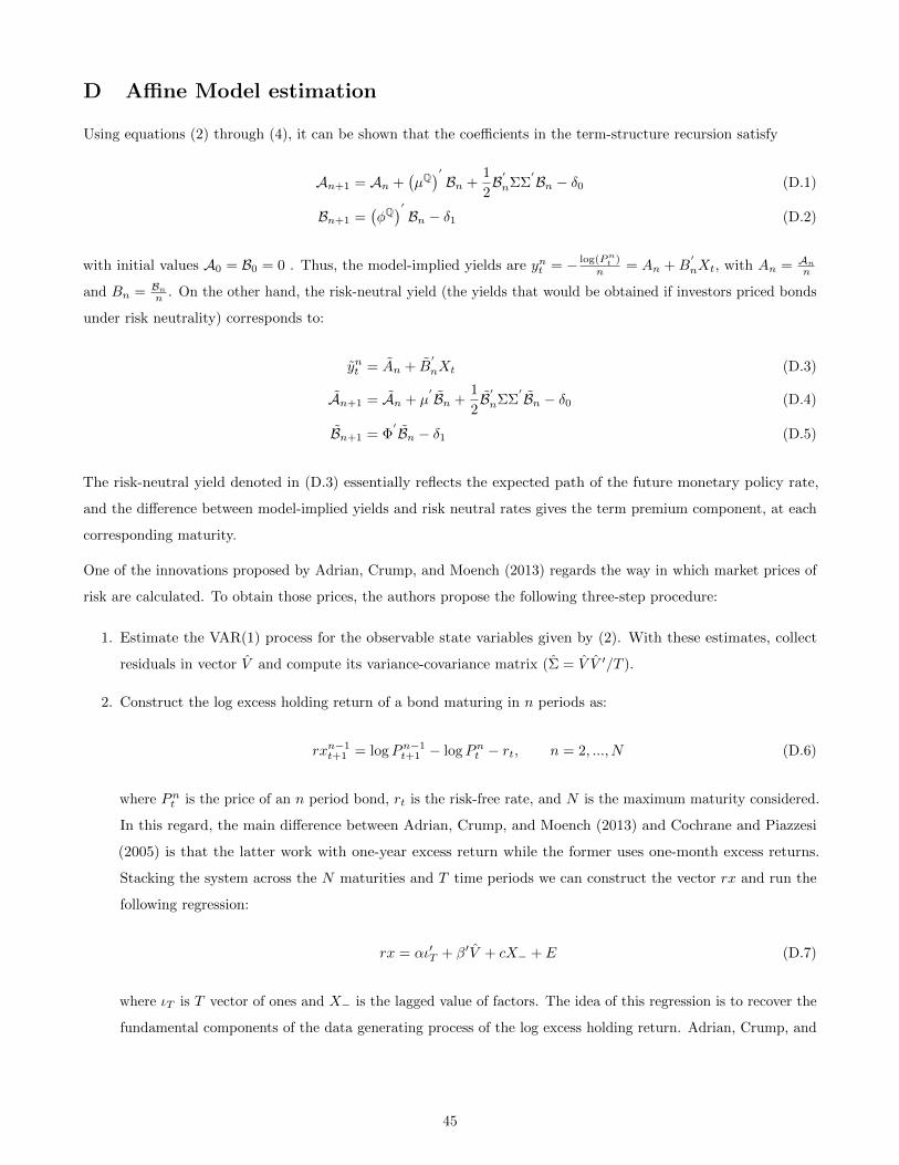
D Affine Model estimation

Using equations (2) through (4), it can be shown that the coefficients in the term-structure recursion satisfy

An+1 = An +(µQ)′ Bn +

1

2B′

nΣΣ′Bn − δ0 (D.1)

Bn+1 =(φQ)′Bn − δ1 (D.2)

with initial values A0 = B0 = 0 . Thus, the model-implied yields are ynt = − log(Pnt )

n = An +B′

nXt, with An = An

n

and Bn = Bn

n . On the other hand, the risk-neutral yield (the yields that would be obtained if investors priced bonds

under risk neutrality) corresponds to:

ynt = An + B′

nXt (D.3)

An+1 = An + µ′Bn +

1

2B′

nΣΣ′Bn − δ0 (D.4)

Bn+1 = Φ′Bn − δ1 (D.5)

The risk-neutral yield denoted in (D.3) essentially reflects the expected path of the future monetary policy rate,

and the difference between model-implied yields and risk neutral rates gives the term premium component, at each

corresponding maturity.

One of the innovations proposed by Adrian, Crump, and Moench (2013) regards the way in which market prices of

risk are calculated. To obtain those prices, the authors propose the following three-step procedure:

1. Estimate the VAR(1) process for the observable state variables given by (2). With these estimates, collect

residuals in vector V and compute its variance-covariance matrix (Σ = V V ′/T ).

2. Construct the log excess holding return of a bond maturing in n periods as:

rxn−1t+1 = logPn−1

t+1 − logPnt − rt, n = 2, ..., N (D.6)

where Pnt is the price of an n period bond, rt is the risk-free rate, and N is the maximum maturity considered.

In this regard, the main difference between Adrian, Crump, and Moench (2013) and Cochrane and Piazzesi

(2005) is that the latter work with one-year excess return while the former uses one-month excess returns.

Stacking the system across the N maturities and T time periods we can construct the vector rx and run the

following regression:

rx = αι′T + β′V + cX− + E (D.7)

where ιT is T vector of ones and X− is the lagged value of factors. The idea of this regression is to recover the

fundamental components of the data generating process of the log excess holding return. Adrian, Crump, and

45

Moench (2013) shows that the decomposition of these returns can be written as:

rx = Expected return + Priced return innovation + Return pricing error

After running (D.7), collect residuals in the N × T matrix E and estimate the return pricing error variance as

σ2 = tr(EE′)/NT .

3. Using the estimated parameters in (D.7), compute the market prices of risk as:

λ0 = (ββ′)−1β[a+1

2(B∗vec(Σ) + σ2)] (D.8)

λ1 = (ββ′)−1βc (D.9)

where B∗ = [vec(β1β1′), ..., vec(βNβN′)]′ and βi is the covariance between log excess holding return at maturity

n and the VAR innovations.

With this procedure, we are able to solve equations (D.1) through (D.5). The difference between fitted yields and

risk-neutral yields corresponds to the term premium component.

46

Previous volumes in this series

718 May 2018

Breaking the trilemma: the effects of financial regulations on foreign assets

David Perez-Reyna and Mauricio Villamizar-Villegas

717 May 2018

Financial and price stability in emerging markets: the role of the interest rate

Lorenzo Menna and Martin Tobal

716 April 2018

Macro-financial linkages: the role of liquidity dependence

Alexey Ponomarenko, Anna Rozhkova and Sergei Seleznev

715 April 2018

A time series model of interest rates with the effective lower bound

Benjamin K Johannsen and Elmar Mertens

714 April 2018

Do interest rates play a major role in monetary policy transmission in China?

Güneş Kamber and Madhusudan Mohanty

713 April 2018

Inflation and professional forecast dynamics: an evaluation of stickiness, persistence, and volatility

Elmar Mertens and James M. Nason

712 March 2018

Firms’ credit risk and the onshore transmission of the global financial cycle

Ramon Moreno and Jose Maria Serena-Garralda

711 March 2018

Credit supply and productivity growth Francesco Manaresi and Nicola Pierri

710 March 2018

Exchange Rate Appreciations and Corporate Risk Taking

Sebnem Kalemli-Ozcan, Xiaoxi Liu and Ilhyock Shim

709 March 2018

Does sovereign risk in local and foreign currency differ?

Marlene Amstad, Frank Packer and Jimmy Shek

708 March 2018

Business Models and Dollar Funding of Global Banks

Iñaki Aldasoro, Torsten Ehlers and Egemen Eren

707 March 2018

Global imbalances from a stock perspective. The asymmetry between creditors and debtors

Enrique Alberola, Ángel Estrada and Francesca Viani

706 March 2018

Monetary policy in the grip of a pincer movement

Claudio Borio, Piti Disyatat, Mikael Juselius and Phurichai Rungcharoenkitkul

705 February 2018

An explanation of negative swap spreads: demand for duration from underfunded pension plans

Sven Klingler and Suresh Sundaresan

704 February 2018

Are credit rating agencies discredited? Measuring market price effects from agency sovereign debt announcements

Mahir Binici, Michael Hutchison and Evan Weicheng Miao

All volumes are available on our website www.bis.org.