cf-5 bank hapoalim jul-2001 zvi wiener 02-588-3049 mswiener/zvi.html computational finance
Post on 20-Dec-2015
220 views
TRANSCRIPT

CF-5 Bank Hapoalim Jul-2001
Zvi Wiener
02-588-3049http://pluto.mscc.huji.ac.il/~mswiener/zvi.html
Computational Finance
CF-5 Bank Hapoalim Jul-2001
Following T. Bjork, ch. 15
Arbitrage Theory in Continuous Time
Bonds and Interest Rates
CF5 slide 3Zvi Wiener
Bonds and Interest Rates
Zero coupon bond = pure discount bond
T-bond, denote its price at time t by p(t,T).
principal = face value,
coupon bond - equidistant payments as a % of the face value, fixed or floating coupons.
CF5 slide 4Zvi Wiener
Assumptions
• There exists a frictionless market for T-
bonds for every T > 0
• p(t, t) =1 for every t
• for every t the price p(t, T) is differentiable
with respect to T.
CF5 slide 5Zvi Wiener
Interest Rates
Let t < S < T, what is IR for [S, T]?
• at time t sell one S-bond, get p(t, S)
• buy p(t, S)/p(t,T) units of T-bond
• cashflow at t is 0
• cashflow at S is -$1
• cashflow at T is p(t, S)/p(t,T)
the forward rate can be calculated ...
CF5 slide 6Zvi Wiener
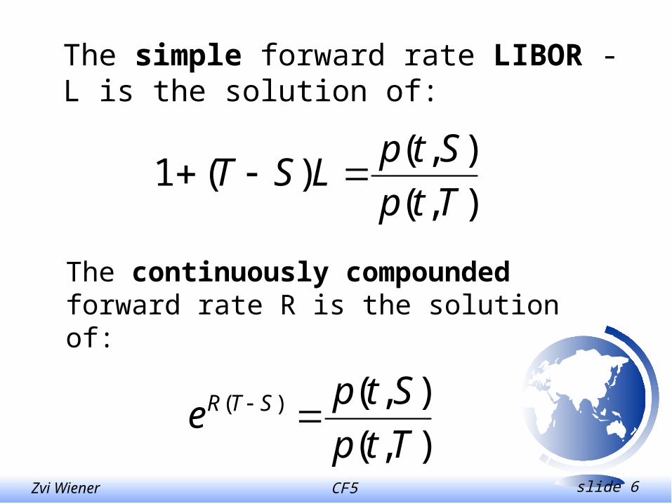
The simple forward rate LIBOR - L is the solution of:
),(
),()(1
Ttp
StpLST
The continuously compounded forward rate R is the solution of:
),(
),()(
Ttp
Stpe STR
CF5 slide 7Zvi Wiener
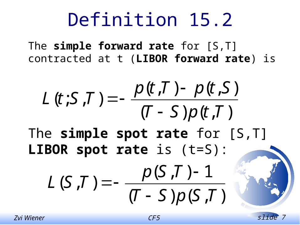
Definition 15.2
The simple forward rate for [S,T] contracted at t (LIBOR forward rate) is
),()(
),(),(),;(
TtpST
StpTtpTStL
The simple spot rate for [S,T] LIBOR spot rate is (t=S):
),()(
1),(),(
TSpST
TSpTSL
CF5 slide 8Zvi Wiener
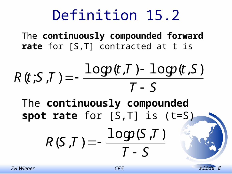
Definition 15.2
The continuously compounded forward rate for [S,T] contracted at t is
ST
StpTtpTStR
),(log),(log
),;(
The continuously compounded spot rate for [S,T] is (t=S)
ST
TSpTSR
),(log),(
CF5 slide 9Zvi Wiener
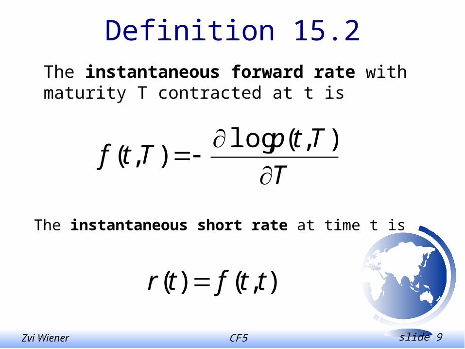
Definition 15.2
The instantaneous forward rate with maturity T contracted at t is
T
TtpTtf
),(log
),(
The instantaneous short rate at time t is
),()( ttftr
CF5 slide 10Zvi Wiener
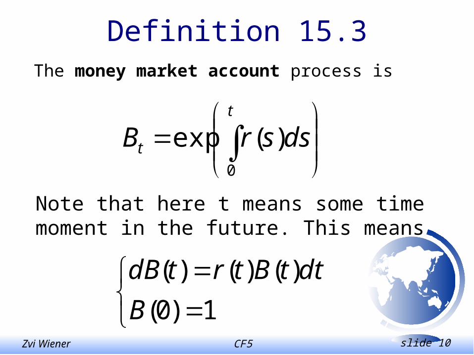
Definition 15.3The money market account process is
t
t dssrB0
)(exp
Note that here t means some time moment in the future. This means
1)0(
)()()(
B
dttBtrtdB
CF5 slide 11Zvi Wiener
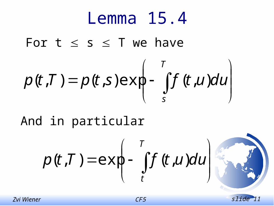
Lemma 15.4For t s T we have
T
s
duutfstpTtp ),(exp),(),(
And in particular
T
t
duutfTtp ),(exp),(
CF5 slide 12Zvi Wiener
Models of Bond Market
• Specify the dynamic of short rate
• Specify the dynamic of bond prices
• Specify the dynamic of forward rates
CF5 slide 13Zvi Wiener
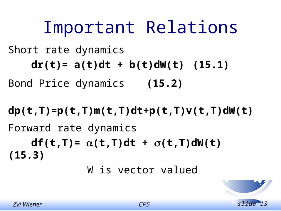
Important RelationsShort rate dynamics
dr(t)= a(t)dt + b(t)dW(t) (15.1)
Bond Price dynamics (15.2)
dp(t,T)=p(t,T)m(t,T)dt+p(t,T)v(t,T)dW(t)
Forward rate dynamics
df(t,T)= (t,T)dt + (t,T)dW(t) (15.3)
W is vector valued
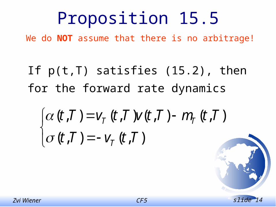
CF5 slide 14Zvi Wiener
Proposition 15.5We do NOT assume that there is no arbitrage!
),(),(
),(),(),(),(
TtvTt
TtmTtvTtvTt
T
TT
If p(t,T) satisfies (15.2), then for the forward
rate dynamics
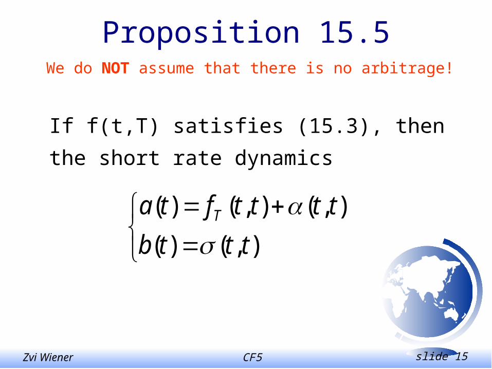
CF5 slide 15Zvi Wiener
Proposition 15.5We do NOT assume that there is no arbitrage!
),()(
),(),()(
tttb
ttttfta T
If f(t,T) satisfies (15.3), then the short rate
dynamics
CF5 slide 16Zvi Wiener
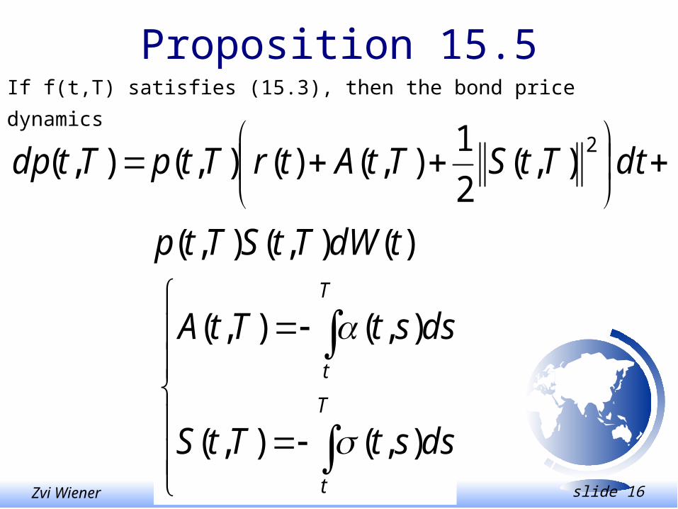
Proposition 15.5
)(),(),(
),(2
1),()(),(),(
2
tdWTtSTtp
dtTtSTtAtrTtpTtdp
If f(t,T) satisfies (15.3), then the bond price dynamics
T
t
T
t
dsstTtS
dsstTtA
),(),(
),(),(
CF5 slide 17Zvi Wiener
Proof of Proposition 15.5Left as an exercise …
CF5 slide 18Zvi Wiener
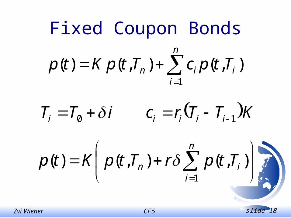
Fixed Coupon Bonds
n
iiin TtpcTtpKtp
1
),(),()(
n
iin TtprTtpKtp
1
),(),()(
KTTrciTT iiiii 10
CF5 slide 19Zvi Wiener
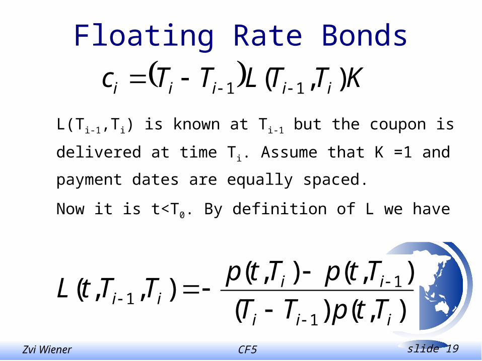
Floating Rate Bonds
KTTLTTc iiiii ),( 11
L(Ti-1,Ti) is known at Ti-1 but the coupon is
delivered at time Ti. Assume that K =1 and
payment dates are equally spaced.
Now it is t<T0. By definition of L we have
),()(
),(),(),,(
1
11
iii
iiii TtpTT
TtpTtpTTtL
CF5 slide 20Zvi Wiener
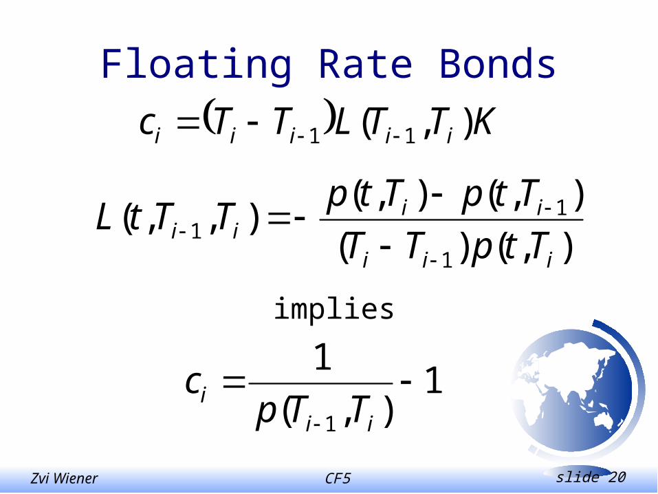
Floating Rate Bonds
1),(
1
1
ii
i TTpc
KTTLTTc iiiii ),( 11
),()(
),(),(),,(
1
11
iii
iiii TtpTT
TtpTtpTTtL
implies
CF5 slide 21Zvi Wiener
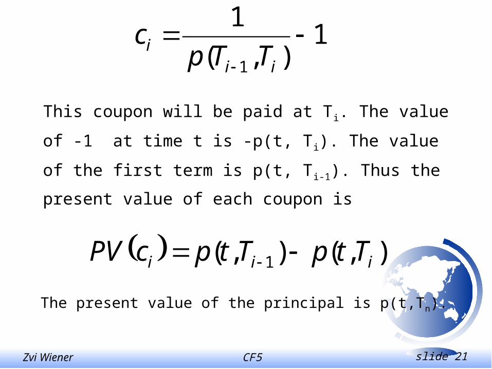
1),(
1
1
ii
i TTpc
This coupon will be paid at Ti. The value of -1 at
time t is -p(t, Ti). The value of the first term is
p(t, Ti-1). Thus the present value of each coupon
is
),(),( 1 iii TtpTtpcPV
The present value of the principal is p(t,Tn).
CF5 slide 22Zvi Wiener
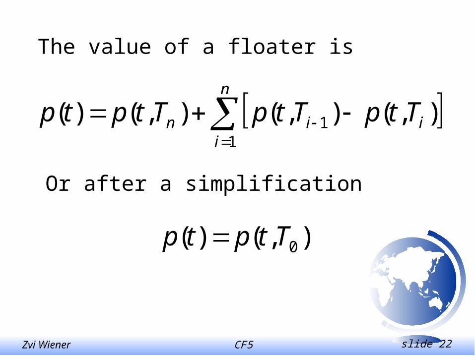
The value of a floater is
n
iiin TtpTtpTtptp
11 ),(),(),()(
),()( 0Ttptp
Or after a simplification

CF5 slide 23Zvi Wiener
Forward Swap Settled in Arrears
K - principal, R - swap rate,
rates are set at dates T0, T1, … Tn-1 and paid at
dates T1, … Tn.
T0 T1 Tn-1 Tn
CF5 slide 24Zvi Wiener
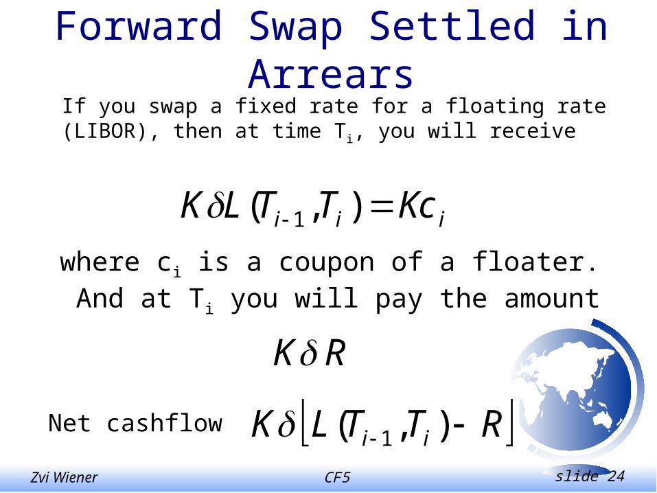
Forward Swap Settled in Arrears
If you swap a fixed rate for a floating rate (LIBOR), then at time Ti, you will receive
iii KcTTLK ),( 1where ci is a coupon of a floater. And at Ti you will pay the amount
RK
Net cashflow RTTLK ii ),( 1

CF5 slide 25Zvi Wiener
Forward Swap Settled in Arrears
At t < T0 the value of this payment is
),()1(),( 1 ii TtpRKTtKp
The total value of the swap at time t is then
n
iii TtpRTtpKt
11 ),()1(),()(
CF5 slide 26Zvi Wiener
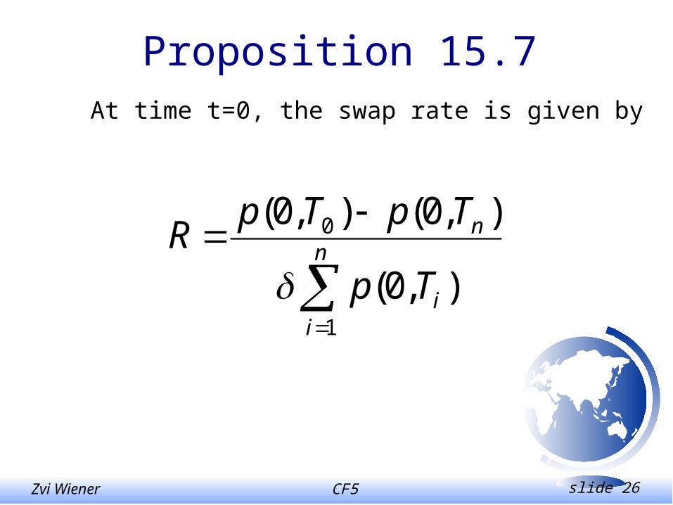
Proposition 15.7
At time t=0, the swap rate is given by
n
ii
n
Tp
TpTpR
1
0
),0(
),0(),0(
CF5 slide 27Zvi Wiener
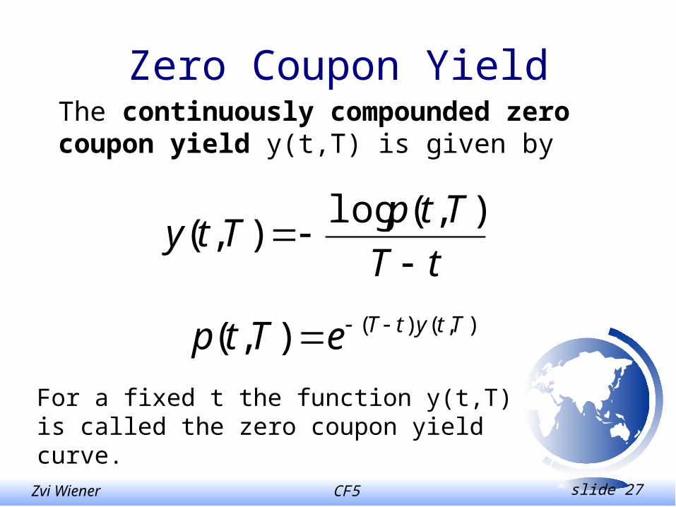
Zero Coupon YieldThe continuously compounded zero coupon yield y(t,T) is given by
tT
TtpTty
),(log),(
),()(),( TtytTeTtp
For a fixed t the function y(t,T) is called the zero coupon yield curve.
CF5 slide 28Zvi Wiener
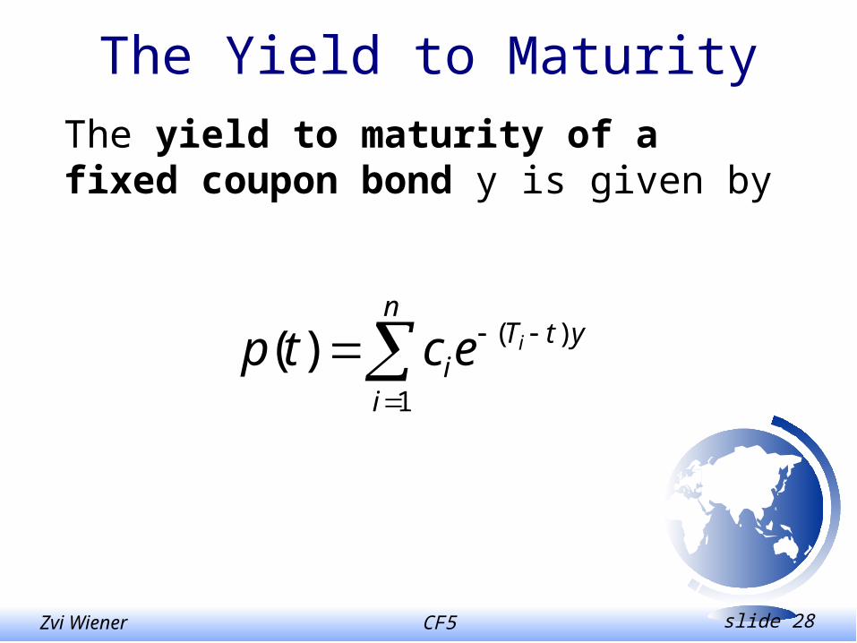
The Yield to Maturity
The yield to maturity of a fixed coupon bond y is given by
n
i
ytTi
iectp1
)()(
CF5 slide 29Zvi Wiener
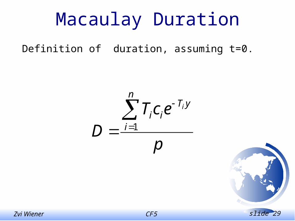
Macaulay Duration
Definition of duration, assuming t=0.
p
ecTD
n
i
yTii
i
1
CF5 slide 30Zvi Wiener
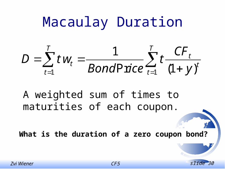
Macaulay Duration
What is the duration of a zero coupon bond?
T
tt
tT
tt y
CFt
iceBondwtD
11 )1(Pr
1
A weighted sum of times to maturities of each coupon.
CF5 slide 31Zvi Wiener
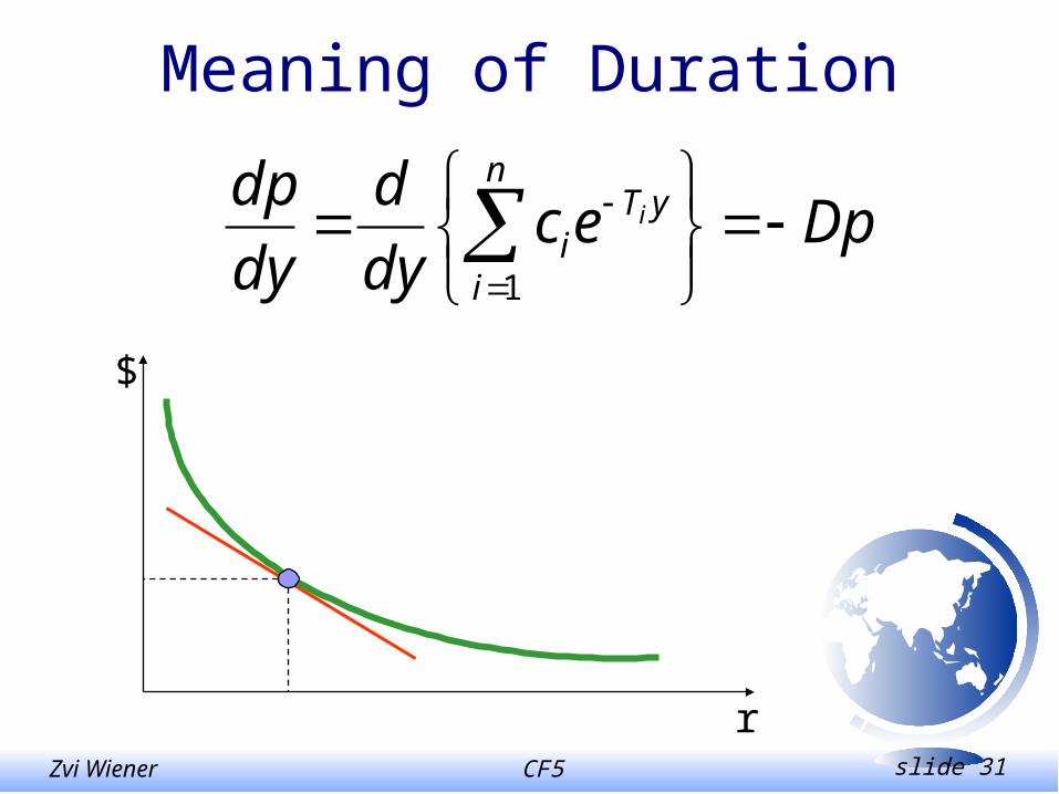
Meaning of Duration
Dpecdy
d
dy
dp n
i
yTi
i
1
r
$
CF5 slide 32Zvi Wiener
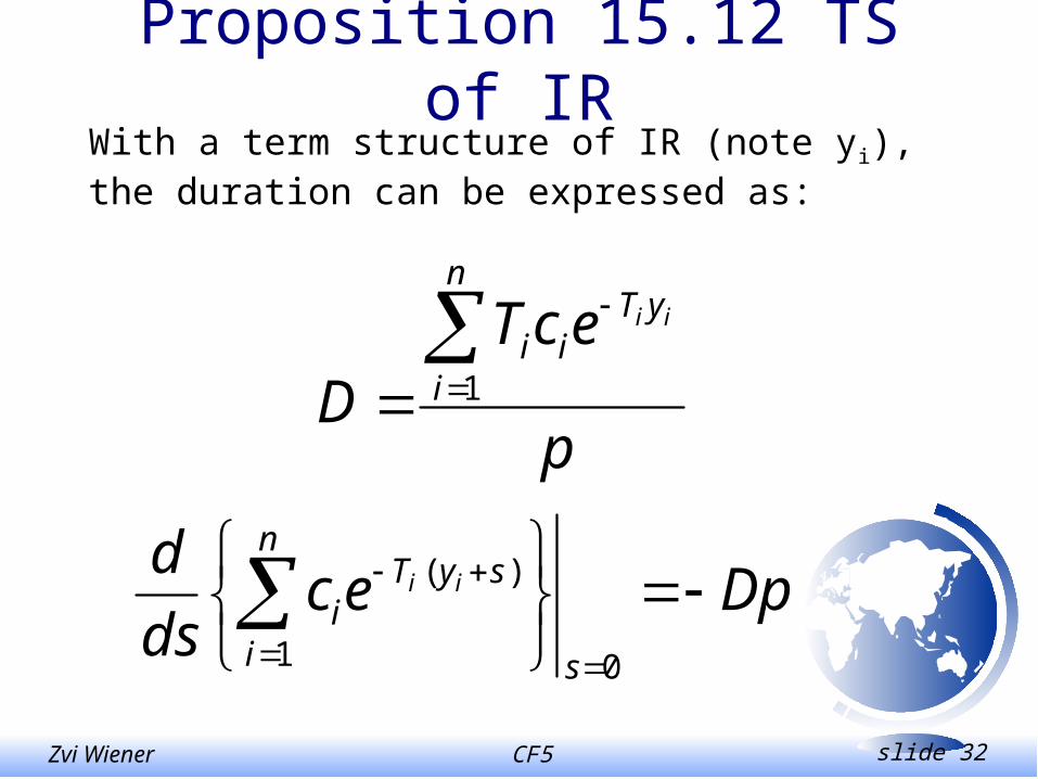
Proposition 15.12 TS of IRWith a term structure of IR (note yi), the duration can be expressed as:
Dpecds
d
s
n
i
syTi
ii
01
)(
p
ecTD
n
i
yTii
ii
1
CF5 slide 33Zvi Wiener
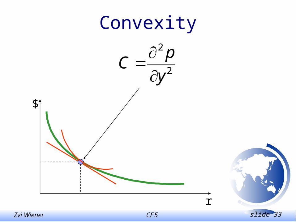
Convexity
r
$
2
2
y
pC
CF5 slide 34Zvi Wiener
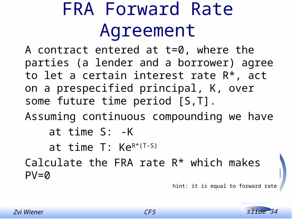
FRA Forward Rate Agreement
A contract entered at t=0, where the parties (a lender and a borrower) agree to let a certain interest rate R*, act on a prespecified principal, K, over some future time period [S,T].
Assuming continuous compounding we have
at time S: -K
at time T: KeR*(T-S)
Calculate the FRA rate R* which makes PV=0hint: it is equal to forward rate
CF5 slide 35Zvi Wiener
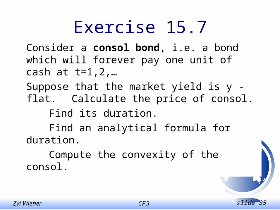
Exercise 15.7Consider a consol bond, i.e. a bond which will forever pay one unit of cash at t=1,2,…
Suppose that the market yield is y - flat. Calculate the price of consol.
Find its duration.
Find an analytical formula for duration.
Compute the convexity of the consol.
CF-5 Bank Hapoalim Jul-2001
Following T. Bjork, ch. 19
Arbitrage Theory in Continuous Time
Change of Numeraire
CF5 slide 37Zvi Wiener
Change of Numeraire
P - the objective probability measure,
Q - the risk-neutral martingale measure,
We will introduce a new class of measures such that Q is a member of this class.
CF5 slide 38Zvi Wiener
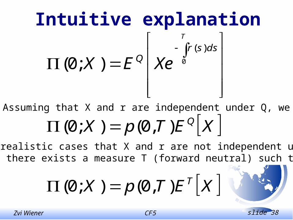
Intuitive explanation
T
dssrQ XeEX 0
)(
);0(
XETpX Q),0();0( Assuming that X and r are independent under Q, we get
In all realistic cases that X and r are not independent under Q.However there exists a measure T (forward neutral) such that
XETpX T),0();0(

CF5 slide 39Zvi Wiener
Risk Neutral Measure
Is such a measure Q that for every choice of price process (t) of a traded asset the following quotient is a Q-martingale.
)(
)(
tB
t
Note that we have divided the asset
price (t) by a numeraire B(t).

CF5 slide 40Zvi Wiener
Conjecture 19.1.1For a given financial market and any asset price process S0(t) there exists a probability measure Q0 such that for any other asset (t)/S0(t) is a Q0-martingale.
For example one can take p(t,T) (fixed T) as S0(t) then there exists a probability measure QT such that for any other asset (t)/p(t,T) is a QT-martingale.
CF5 slide 41Zvi Wiener
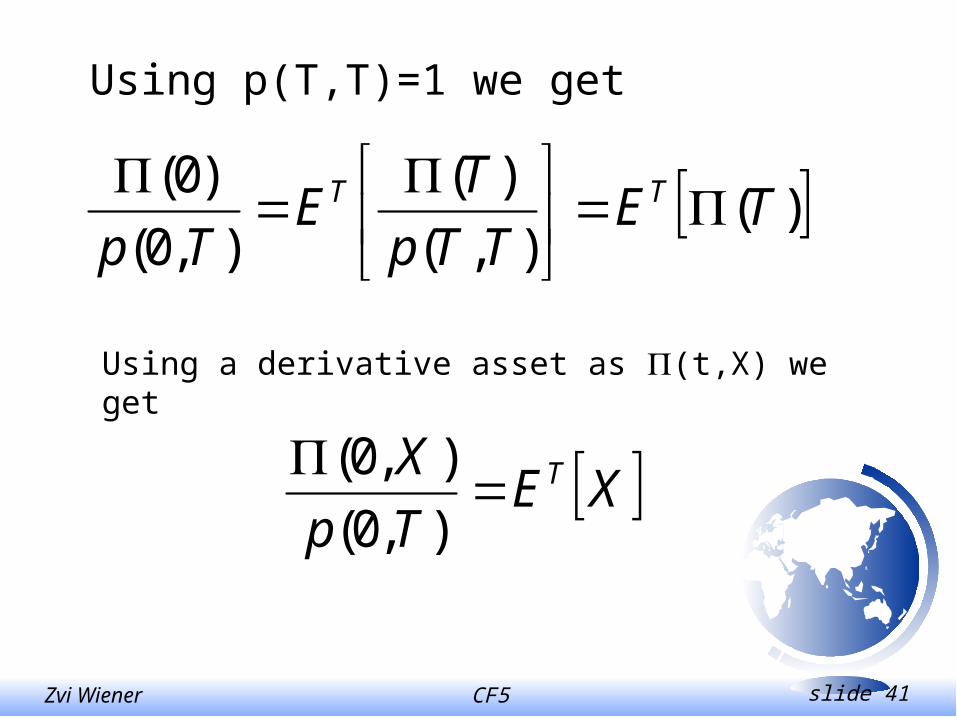
Using p(T,T)=1 we get
)(),(
)(
),0(
)0(TE
TTp
TE
TpTT
Using a derivative asset as (t,X) we get
XETp
X T
),0(
),0(

CF5 slide 42Zvi Wiener
Assumption 19.2.1
Denote an observable k+1 dimensional process X=(X1, …, Xk, Xk+1) where
Xk+1(t)=r(t) (short term IR)
Denote by Q a fixed martingale measure under which the dynamics is:
dXi(t)=i(t,X(t))dt + i(t,X(t))dW(t), i=1,…,k+1
A risk free asset (money market account):
dB(t)=r(t)B(t)dt
CF5 slide 43Zvi Wiener
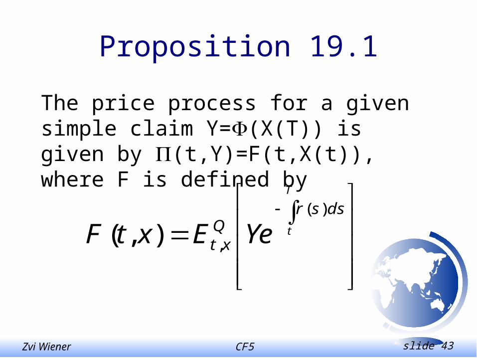
Proposition 19.1
The price process for a given simple claim Y=(X(T)) is given by (t,Y)=F(t,X(t)), where F is defined by
T
t
dssrQ
xt YeExtF)(
,),(

CF-5 Bank Hapoalim Jul-2001
Zvi Wiener
02-588-3049http://pluto.mscc.huji.ac.il/~mswiener/zvi.html
Practical Numeraire Approach
CF5 slide 45Zvi Wiener
Options with uncertain strikeStock option with strike fixed in foreign currency.How it can be priced?
Margarbe 78 or Numeraire approach
1. Price it using this currency as a numeraire.foreign interest rateforeign current priceforeign volatility!
2. Translate the resulting price into SHEKELS using the current exchange rate.
CF5 slide 46Zvi Wiener
Options with uncertain strike
Endowment warrants
strike is increasing with short term IR.
strike is decreasing when a dividend is paid
What is an appropriate numeraire?
A closed Money Market account.
Result – price by standard BS but with 0 dividends and 0 IR.

CF5 slide 47Zvi Wiener
Options with uncertain strike
An option to choose by some date between dollar
and CPI indexing (may be with some interest).
Margrabe can be used or one can price a simple
CPI option in terms of an American investor and
then translate it to SHEKELS.
CF5 slide 48Zvi Wiener
Convertible Bonds
A convertible bond typically includes an option to convert it into some amount of ordinary shares.
This can be seen as a package of a regular bond and an option to exchange this regular bond to shares of the company.
If the company does not have traded debt there is a problem of pricing this option.
CF5 slide 49Zvi Wiener
Convertible BondsThis is an option to exchange one asset to another and can be priced with Margrabe approach.
However in order to use this approach one need to know the correlation between the two assets (stock and regular bond).
When there is no market for regular bonds this might be a problem.
CF5 slide 50Zvi Wiener
Convertible BondsAn alternative approach is with a numeraire.
Denote by
St stock price at time t,
Bt price at time t of a regular bond (may be not observable).
CBt price of a convertible bond.
C - value of the conversion option, so that
CB = C(B) + B at any time
CF5 slide 51Zvi Wiener
Convertible BondsNote that C is a decreasing function of B (the higher the strike price, the lower is the option’s value).
This means that as soon as
CBt < St = C(B=0) the right hand side of the following equation (B - an unknown)
CBt = C(Bt) + Bt
has a unique solution.
CF5 slide 52Zvi Wiener
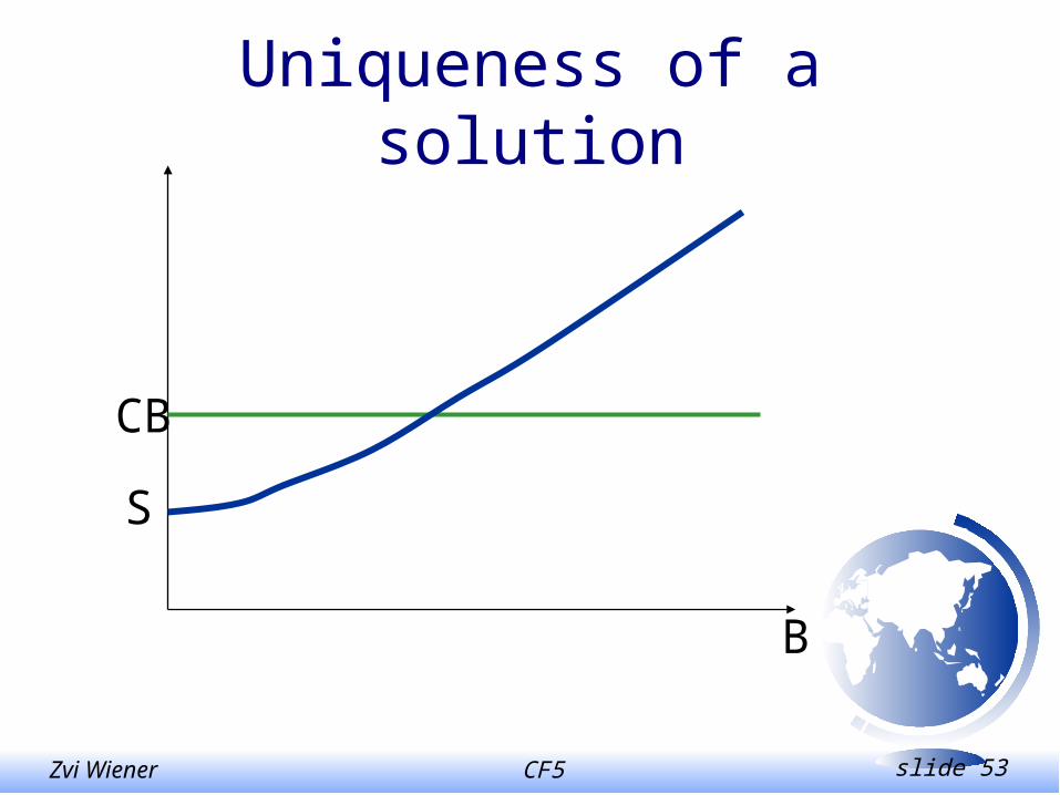
Convertible BondsThe left hand side is a known constant, the right hand side is a sum of two variables.
The first one is decreasing in B, but its derivative is strictly less than one and approaches zero for large B.
The second one is linear with slope one.
This means that as soon as CB>C(B=0)+0=S there exists a unique solution.
CF5 slide 53Zvi Wiener
Uniqueness of a solution
B
CB
S
CF5 slide 54Zvi Wiener
Pricing with known volatility
Let’s use Bt as a numeraire, then the stochastic variable is St/Bt.
Assume that St/Bt has a constant volatility .
Then this option has a fixed strike (in terms of B) and is equivalent to a standard option, which can be priced with BS equation.
Call(St/Bt, T, 1, , r) (in terms of Bt),
the dollar value is then BtCall(St/Bt, T, 1, , r).
CF5 slide 55Zvi Wiener
Pricing with known volatility
This means that when is known the option can be priced easily and consequently the straight bond.
However that we need can not be observed. The solution is in the following procedure.
CF5 slide 56Zvi Wiener
Pricing with known volatility
Assume that is stable but unknown. For any value of we can easily price the option at any date, and hence we can also derive the value of Bt.
Take a sequence of historical data (meaning St and CBt). For any value of we can construct the implied Bt().
Then using these sequence of observations we can check whether the volatility of St/Bt is indeed .
If our guess of was correct this is true.
CF5 slide 57Zvi Wiener
Pricing with known volatility
However there is no reason why some value of will give the same implied historical volatility. This means that we have to solve for such that the implied volatility is equal .
Numerically this can be done easily.
Why there exists a unique solution???
Check monotonicity!!
CF5 slide 58Zvi Wiener
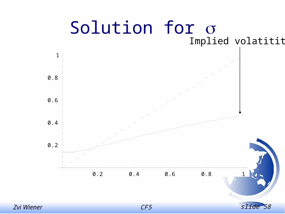
Solution for
0.2 0.4 0.6 0.8 1
0.2
0.4
0.6
0.8
1
Implied volatitity
CF5 slide 59Zvi Wiener
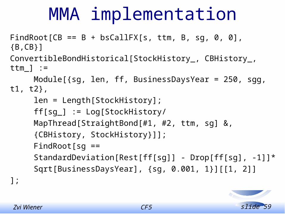
MMA implementationFindRoot[CB == B + bsCallFX[s, ttm, B, sg, 0, 0], {B,CB}]
ConvertibleBondHistorical[StockHistory_, CBHistory_, ttm_] :=
Module[{sg, len, ff, BusinessDaysYear = 250, sgg, t1, t2},
len = Length[StockHistory];
ff[sg_] := Log[StockHistory/
MapThread[StraightBond[#1, #2, ttm, sg] &,
{CBHistory, StockHistory}]];
FindRoot[sg ==
StandardDeviation[Rest[ff[sg]] - Drop[ff[sg], -1]]*
Sqrt[BusinessDaysYear], {sg, 0.001, 1}][[1, 2]]
];

CF5 slide 60Zvi Wiener
20 40 60 80 100
0.9
0.95
1.05
1.1
1.15
Example 1CB
S
B
CF5 slide 61Zvi Wiener
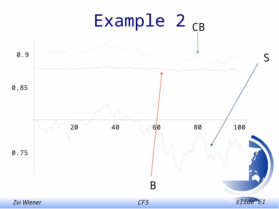
20 40 60 80 100
0.75
0.85
0.9
Example 2 CB
S
B

CF-5 Bank Hapoalim Jul-2001
Zvi Wiener
The Hebrew University of Jerusalem
Value of Value-at-Risk

CF5 slide 63Zvi Wiener
P&L
VaR
1 day
1% probability 1d
1 week
1% probability 1w
CF5 slide 64Zvi Wiener
Model
• Bank’s choice of an optimal system
• Depends on the available capital
• Current and potential capital needs
• Queuing model as a base
CF5 slide 65Zvi Wiener
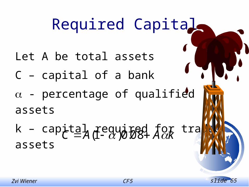
Required Capital
Let A be total assets
C – capital of a bank
- percentage of qualified assets
k – capital required for traded assets
kAAC 08.0)1(
CF5 slide 66Zvi Wiener
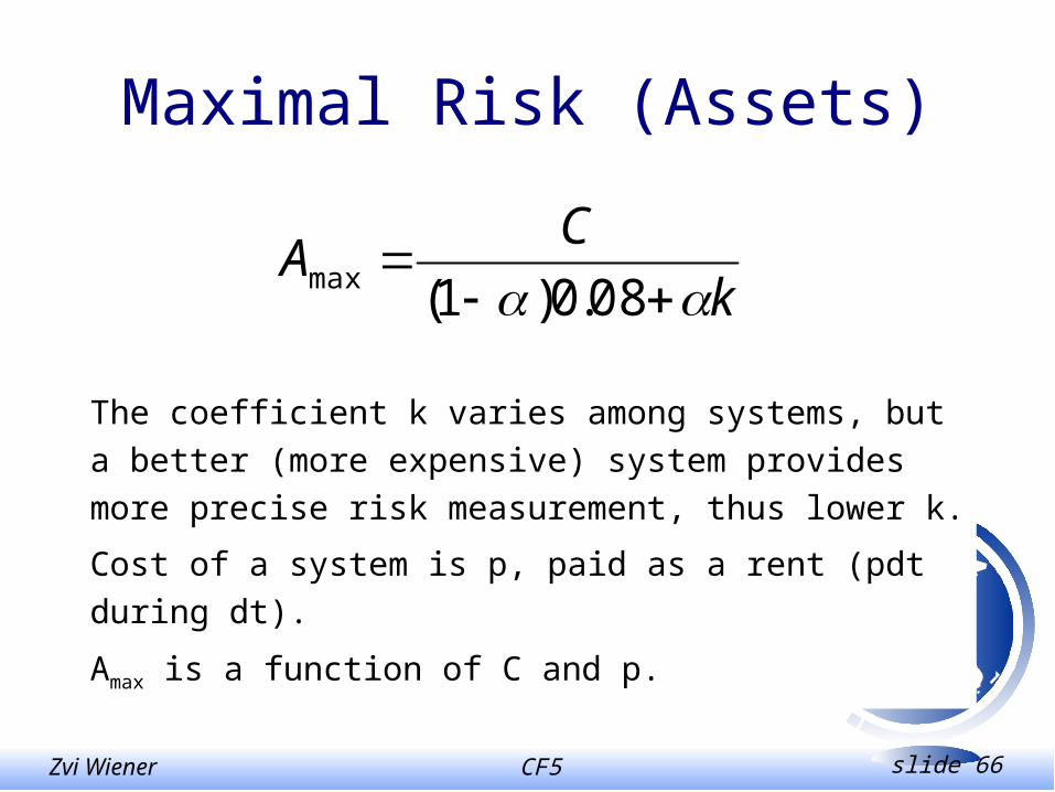
Maximal Risk (Assets)
The coefficient k varies among systems, but a better
(more expensive) system provides more precise risk
measurement, thus lower k.
Cost of a system is p, paid as a rent (pdt during dt).
Amax is a function of C and p.
k
CA
08.0)1(max

CF5 slide 67Zvi Wiener
Risky Projects
Deposits arrive and are withdrawn randomly.
All deposits are of the same size.
Invested according to bank’s policy.
Can not be used if capital requirements are
not satisfied.
CF5 slide 68Zvi Wiener
Arrival of Risky ProjectsWe assume that risky projects arrive randomly (as a Poisson process with density ).
This means that there is a probability dt that during dt one new project arrives.
CF5 slide 69Zvi Wiener
Arrival of Risky ProjectsA new project is undertaken if the bank has enough capital (according to the existing risk measuring system).
We assume that one can NOT raise capital or change systems quickly.
CF5 slide 70Zvi Wiener
Termination of Risky Projects
We assume that each risky project disappears randomly (as a Poisson process with density ).
CF5 slide 71Zvi Wiener
Termination of Risky Projects
We assume that each risky project disappears randomly (as a Poisson process with density ).
This means that there is a probability ndt that during dt one out of n existing projects terminates.
With probability (1-ndt) all existing projects will be active after dt.
CF5 slide 72Zvi Wiener
ProfitWe assume that each existing risky project gives a profit of dt during dt.
Thus when there are n active projects the bank has instantaneous profit (n-p)dt.
CF5 slide 73Zvi Wiener
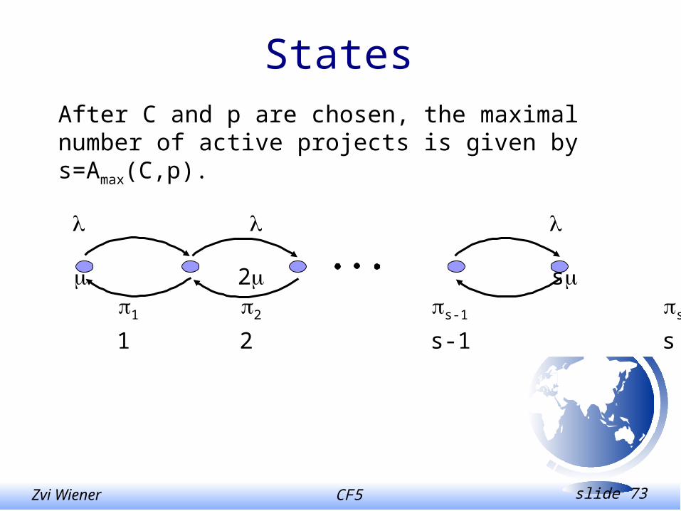
States
After C and p are chosen, the maximal number of active projects is given by s=Amax(C,p).
0 1 2 s-1 s
0 1 2 s-1 s
2 s
CF5 slide 74Zvi Wiener
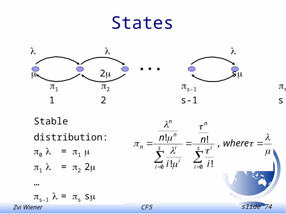
States
0 1 2 s-1 s
0 1 2 s-1 s
2 s
Stable distribution:
0 = 1
1 = 2 2
…
s-1 = s s
where
i
n
i
ns
i
i
n
s
ii
i
n
n
n ,
!
!
!
!
00
CF5 slide 75Zvi Wiener
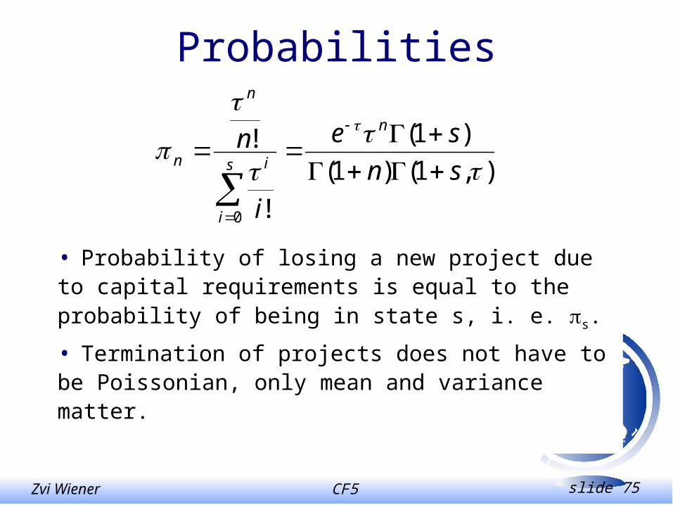
Probabilities
• Probability of losing a new project due to capital requirements is equal to the probability of being in state s, i. e. s.
• Termination of projects does not have to be Poissonian, only mean and variance matter.
),1()1(
)1(
!
!
0
sn
se
i
nn
s
i
i
n
n
CF5 slide 76Zvi Wiener
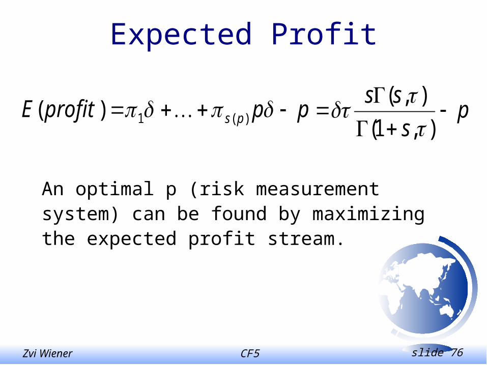
Expected Profit
An optimal p (risk measurement system) can be found by maximizing the expected profit stream.
ppprofitE ps )(1)( ps
ss
),1(
),(
CF5 slide 77Zvi Wiener
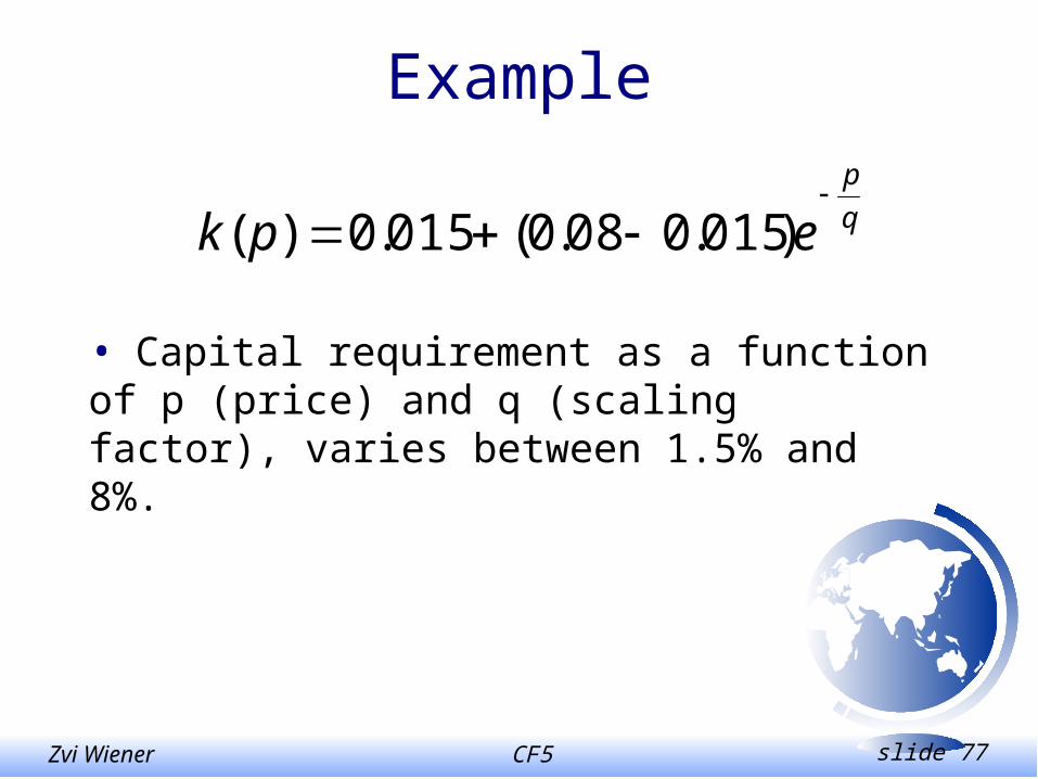
Example
• Capital requirement as a function of p (price) and q (scaling factor), varies between 1.5% and 8%.
q
p
epk
)015.008.0(015.0)(
CF5 slide 78Zvi Wiener
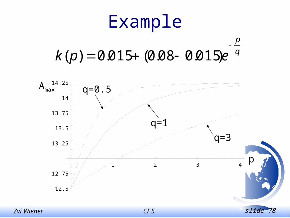
Example
q
p
epk
)015.008.0(015.0)(
1 2 3 4
12.5
12.75
13.25
13.5
13.75
14
14.25q=0.5
q=1
q=3
p
Amax
CF5 slide 79Zvi Wiener
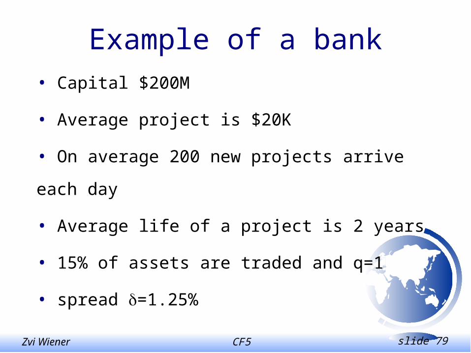
Example of a bank
• Capital $200M
• Average project is $20K
• On average 200 new projects arrive each day
• Average life of a project is 2 years
• 15% of assets are traded and q=1
• spread =1.25%

CF5 slide 80Zvi Wiener
Bank’s profit as a function of cost p. C=$200M, arrival rate 200/d,size $20K, average life 2 yr.,
spread 1.25%, q=1, 15% of assets are traded.
1 2 3 4 5 629.5
30.5
31
31.5
32
32.5
33
rent p
Expected profit
CF5 slide 81Zvi Wiener
rent p
Expected profit
1 2 3 4 5 6
21
22
23
24
25
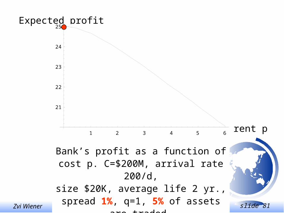
Bank’s profit as a function of cost p. C=$200M, arrival rate 200/d,size $20K, average life 2 yr.,
spread 1%, q=1, 5% of assets are traded.
CF5 slide 82Zvi Wiener
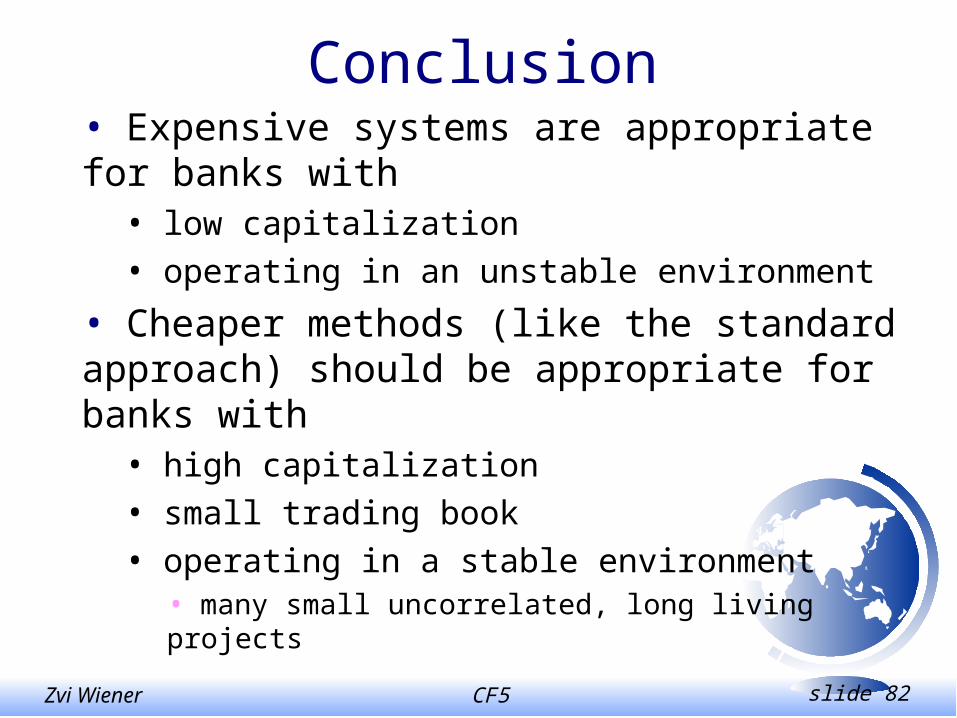
Conclusion• Expensive systems are appropriate for banks with
• low capitalization
• operating in an unstable environment
• Cheaper methods (like the standard approach) should be appropriate for banks with
• high capitalization
• small trading book
• operating in a stable environment• many small uncorrelated, long living projects
CF5 slide 83Zvi Wiener
A simple intuitive and flexible model of
optimal choice of risk measuring method.

CF-5 Bank Hapoalim Jul-2001
Zvi Wiener
02-588-3049http://pluto.mscc.huji.ac.il/~mswiener/zvi.html
DAC
CF5 slide 85Zvi Wiener
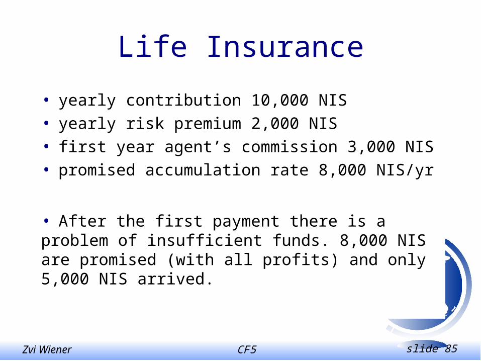
Life Insurance
• yearly contribution 10,000 NIS
• yearly risk premium 2,000 NIS
• first year agent’s commission 3,000 NIS
• promised accumulation rate 8,000 NIS/yr
• After the first payment there is a problem of insufficient funds. 8,000 NIS are promised (with all profits) and only 5,000 NIS arrived.
CF5 slide 86Zvi Wiener
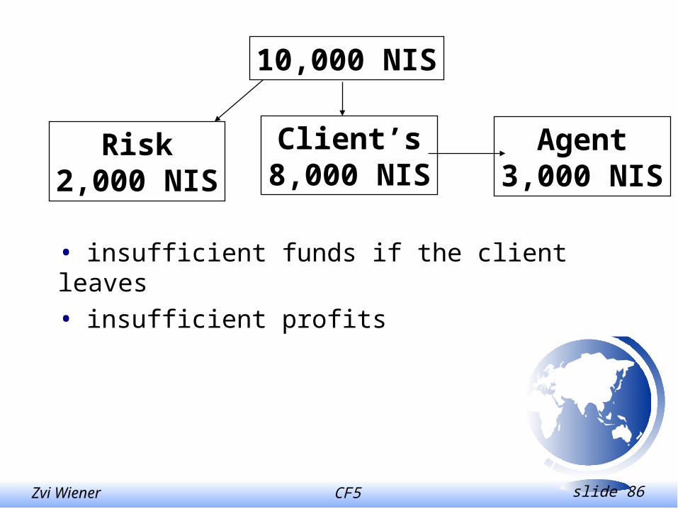
10,000 NIS
Risk2,000 NIS
Client’s8,000 NIS
Agent3,000 NIS
• insufficient funds if the client leaves
• insufficient profits
CF5 slide 87Zvi Wiener
Risk measurement
• The reason to enter this transaction is because of the expected future profits.
• Assume that the program is for 15 years and the probability of leaving such a program is .
• Fees are • 0.6% of the portfolio value each year
• 15% real profit participation
CF5 slide 88Zvi Wiener
Obligations
• The most important question is what are the
obligations?
• The Ministry of Finance should decide
• Transparent to a client
• Accounted as a loan
CF5 slide 89Zvi Wiener
One year example
Assume that the program is for one year only
and there is no possibility to stop payments
before the end.
Initial payment P0, fees lost L0, fixed fee a%
of the final value P1, participation fee b% of
real profits (we ignore real).
Investment policy TA-25 (MAOF).
CF5 slide 90Zvi Wiener
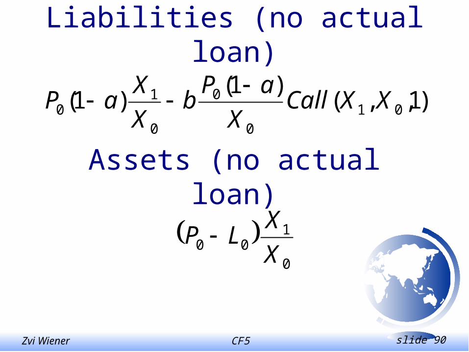
Liabilities (no actual loan)
)1,,()1(
)1( 010
0
0
10 XXCall
X
aPb
X
XaP
Assets (no actual loan)
0
100 X
XLP
CF5 slide 91Zvi Wiener
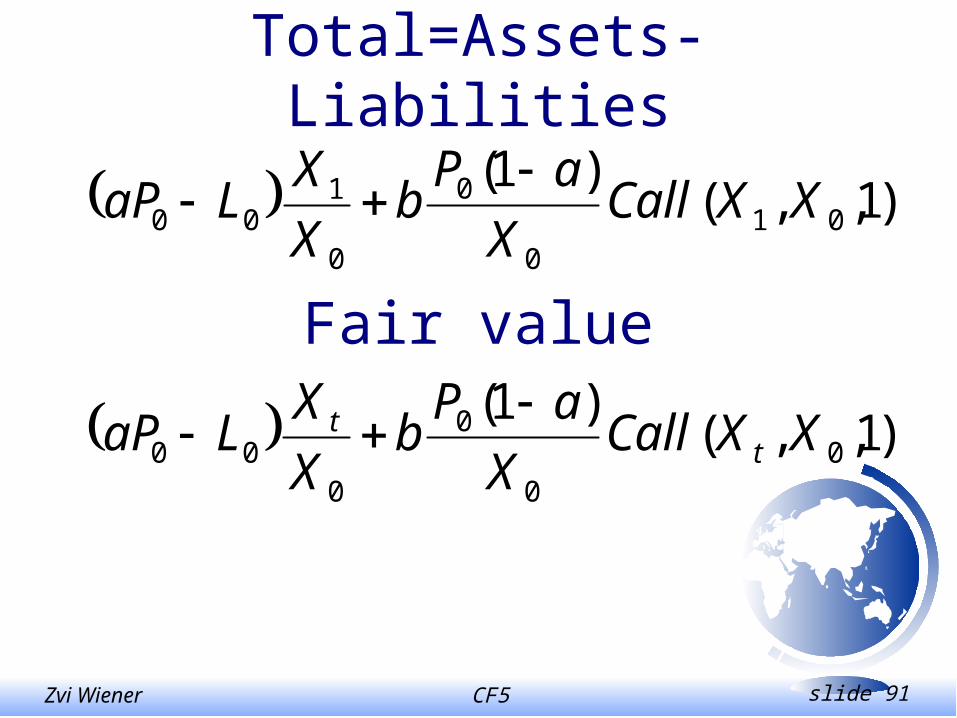
Total=Assets-Liabilities
)1,,()1(
010
0
0
100 XXCall
X
aPb
X
XLaP
Fair value
)1,,()1(
00
0
000 XXCall
X
aPb
X
XLaP t
t
CF5 slide 92Zvi Wiener
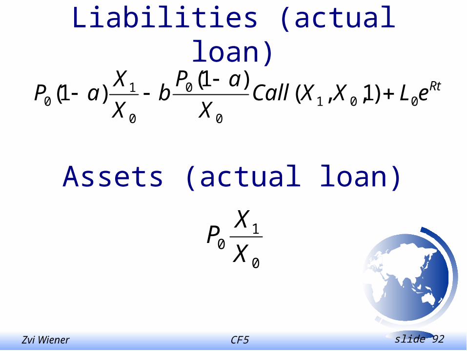
Liabilities (actual loan)
RteLXXCallX
aPb
X
XaP 001
0
0
0
10 )1,,(
)1()1(
Assets (actual loan)
0
10 X
XP
CF5 slide 93Zvi Wiener
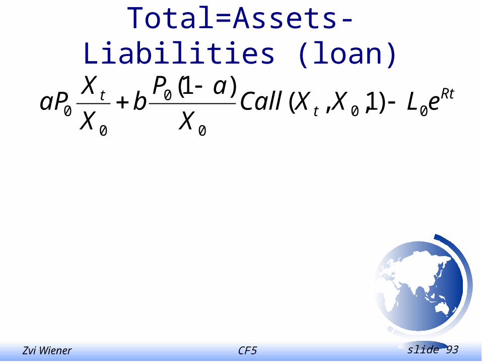
Total=Assets-Liabilities (loan)
Rtt
t eLXXCallX
aPb
X
XaP 00
0
0
00 )1,,(
)1(
CF5 slide 94Zvi Wiener
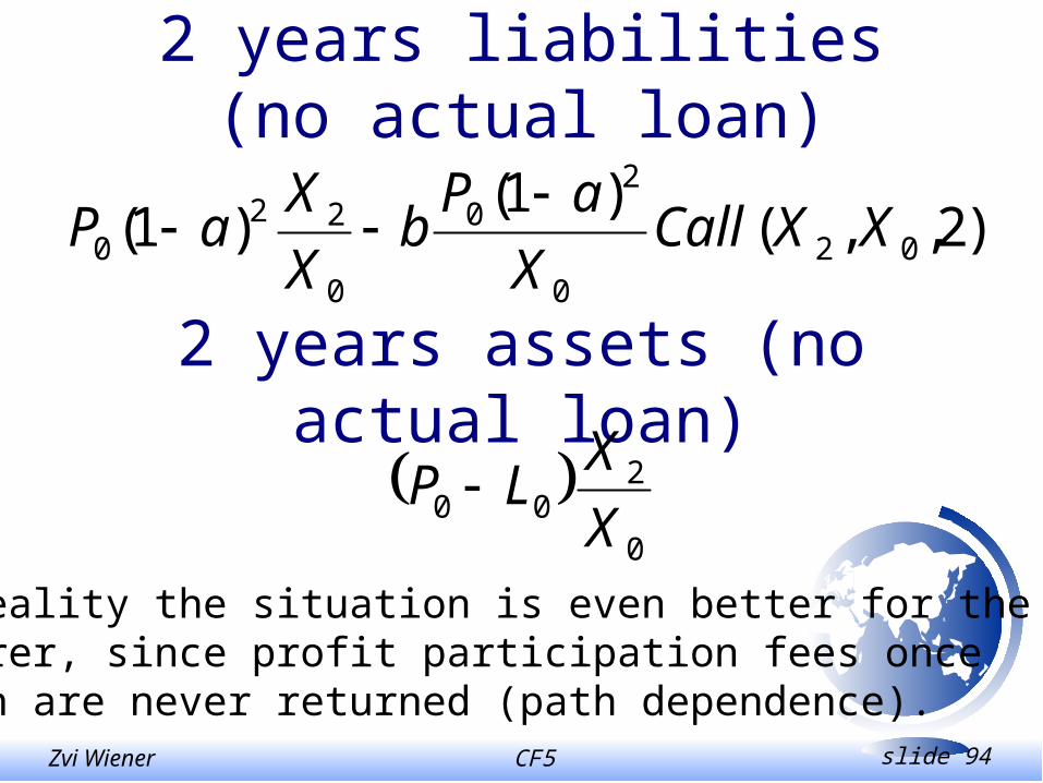
2 years liabilities (no actual loan)
)2,,()1(
)1( 020
20
0
220 XXCall
X
aPb
X
XaP
2 years assets (no actual loan)
0
200 X
XLP
In reality the situation is even better for theinsurer, since profit participation fees oncetaken are never returned (path dependence).
CF5 slide 95Zvi Wiener
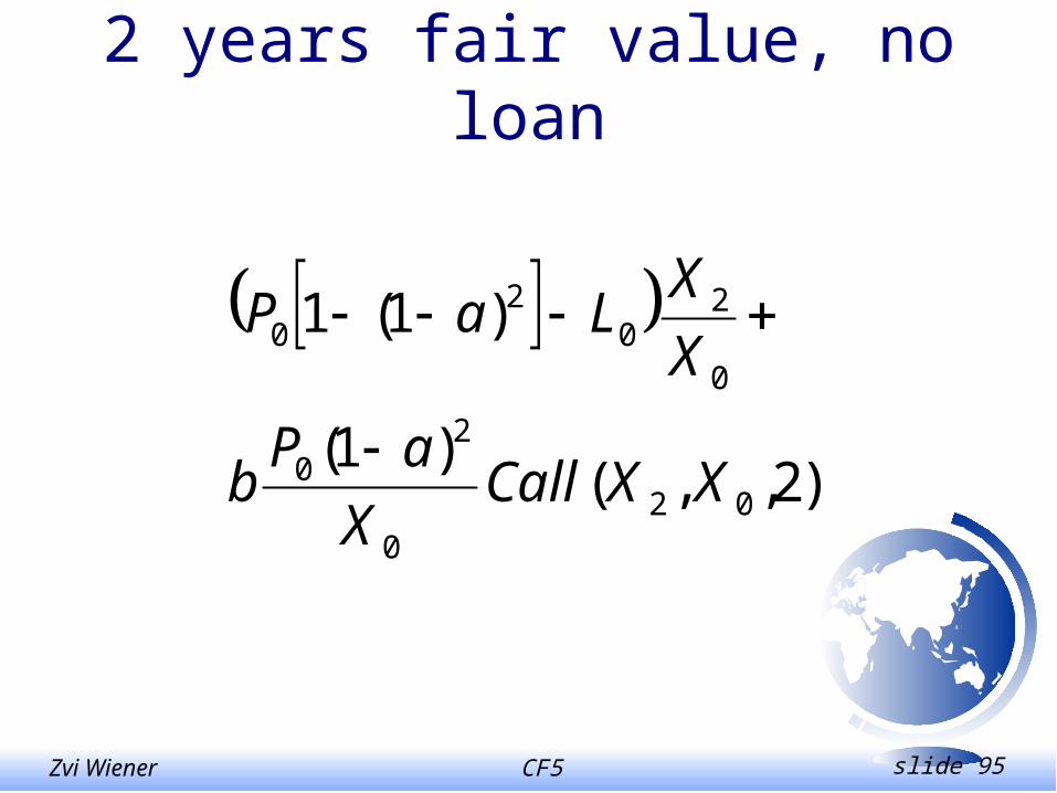
2 years fair value, no loan
)2,,()1(
)1(1
020
20
0
20
20
XXCallX
aPb
X
XLaP
CF5 slide 96Zvi Wiener
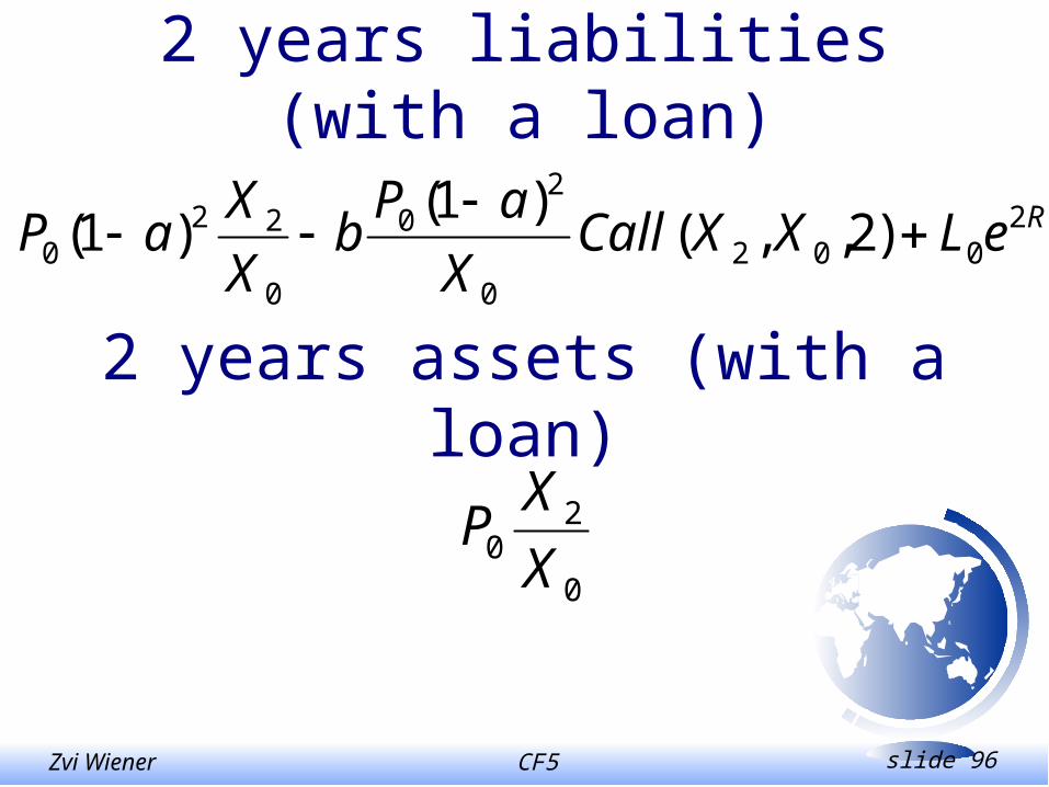
2 years liabilities (with a loan)
ReLXXCallX
aPb
X
XaP 2
0020
20
0
220 )2,,(
)1()1(
2 years assets (with a loan)
0
20 X
XP
CF5 slide 97Zvi Wiener
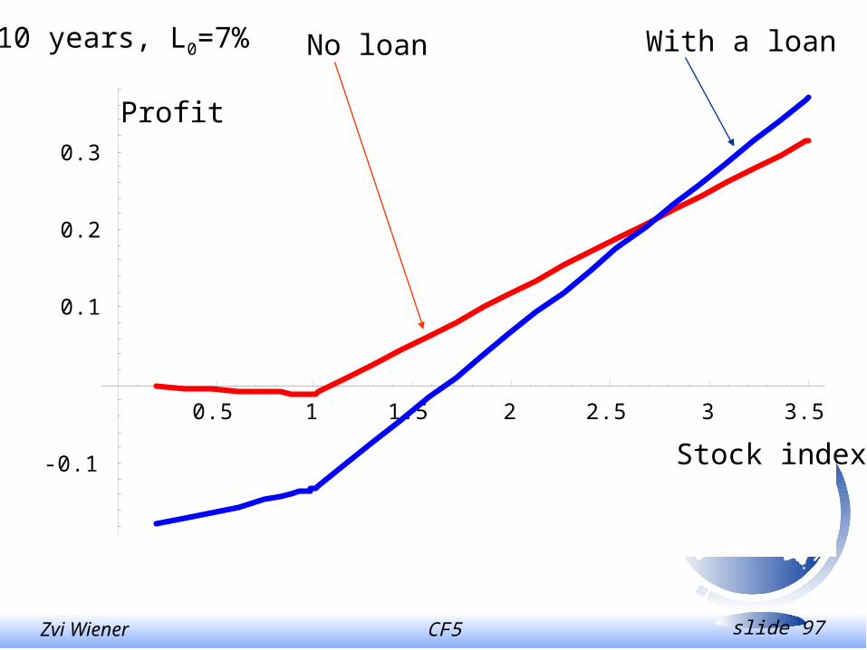
0.5 1 1.5 2 2.5 3 3.5
-0.1
0.1
0.2
0.3
Stock index
Profit
No loan With a loan10 years, L0=7%

CF5 slide 98Zvi Wiener
Partial loan - portion q
nRn
n
nn
qLenXXCallX
aPb
X
XLqaP
),,()1(
)1()1(1
00
0
000
Theoretically q can be negative.

CF5 slide 99Zvi Wiener
Mixed portfolio
When the investment portfolio is a mix one should analyze it in a similar manner. Important: an option on a portfolio is less valuable than a portfolio of options.
Another risk factor - leaving rate should be accounted for by taking actuarial tables as leaving rate.
CF5 slide 100Zvi Wiener
Conclusions
It is a reasonable risk management policy not to take a loan against DAC.
Up to some optimal point it creates a useful hedge to other assets (call options and shares) of the firm.
Intuitively DAC is good when the stock market performs badly and profit participation is valueless. DAC performs bad when the market performs well.