qa-2 frm-garp sep-2001 zvi wiener 02-588-3049 mswiener/zvi.html quantitative analysis 2

QA-2 FRM-GARP Sep-2001

Zvi Wiener

02-588-3049http://pluto.mscc.huji.ac.il/~mswiener/zvi.html

Quantitative Analysis 2

QA-2 FRM-GARP Sep-2001

Fundamentals of Probability

Following Jorion 2001

Zvi Wiener - QA2 slide 3http://www.tfii.org

Random Variables

Values, probabilities.

Distribution function, cumulative probability.

Example: a die with 6 faces.


Random Variables

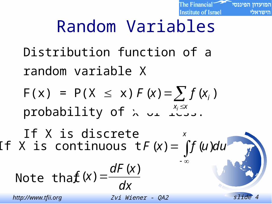
Distribution function of a random variable X

F(x) = P(X x) - the probability of x or less.

If X is discrete then

xx

i

i

xfxF )()(

If X is continuous then

x

duufxF )()(

Note thatdx

xdFxf

)()(


Random Variables

Probability density function of a random

variable X has the following properties

0)( xf

duuf )(1


Multivariate Distribution Functions

Joint distribution function

),(),( 22112112 xXxXPxxF

1 2

2121122112 ),(),(x x

duduuufxxF

Joint density - f12(u1,u2)


Independent variables

)()(),( 22112112 ufufuuf

)()(),( 22112112 uFuFuuF

Credit exposure in a swap depends on two randomvariables: default and exposure.If the two variables are independent one canconstruct the distribution of the credit loss easily.


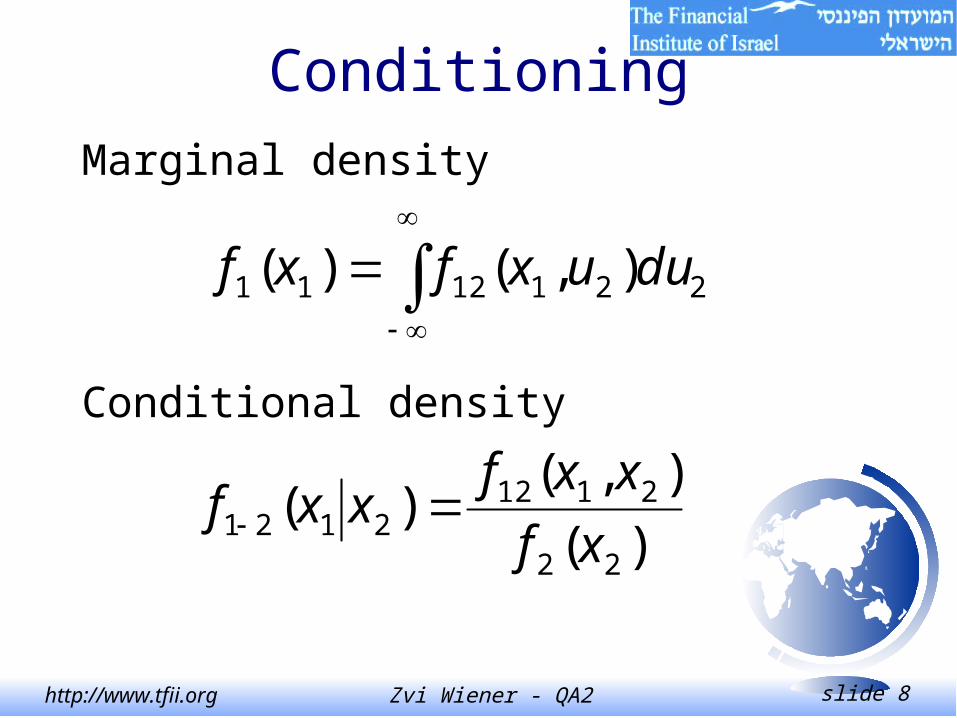
Conditioning

Marginal density

2211211 ),()( duuxfxf

Conditional density

)(

),()(

22

21122121 xf

xxfxxf


MomentsMean = Average = Expected value

dxxxfXE )()(

Variance

dxxfXExXV )()()( 22

VarianceDeviationdardS tan


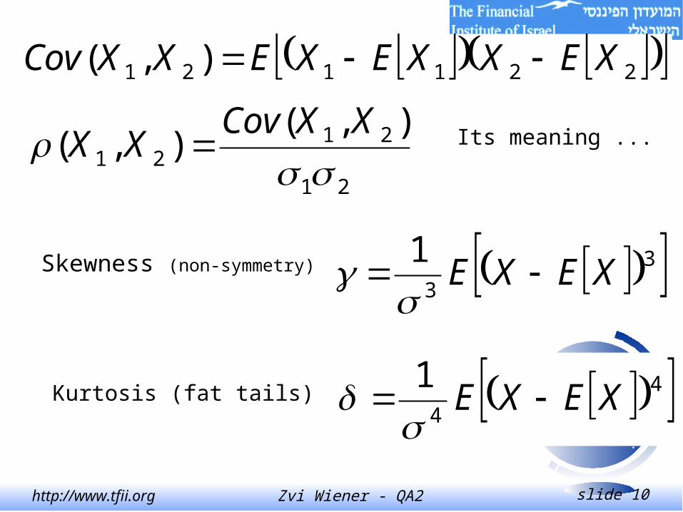
221121 ),( XEXXEXEXXCov

Its meaning ...

3

3

1XEXE

21

2121

),(),(

XXCov

XX

Skewness (non-symmetry)

4

4

1XEXE

Kurtosis (fat tails)


Main properties

)()( XbEabXaE

)()( XbbXa

)()()( 2121 XEXEXXE

),(2)()()( 2122

12

212 XXCovXXXX


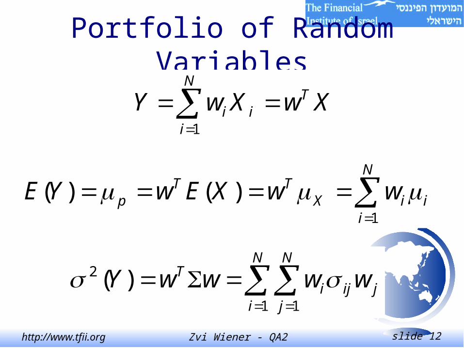
Portfolio of Random Variables

XwXwY TN

iii

1

N

iiiX

TTp wwXEwYE

1

)()(

N

i

N

jjiji

T wwwwY1 1

2 )(


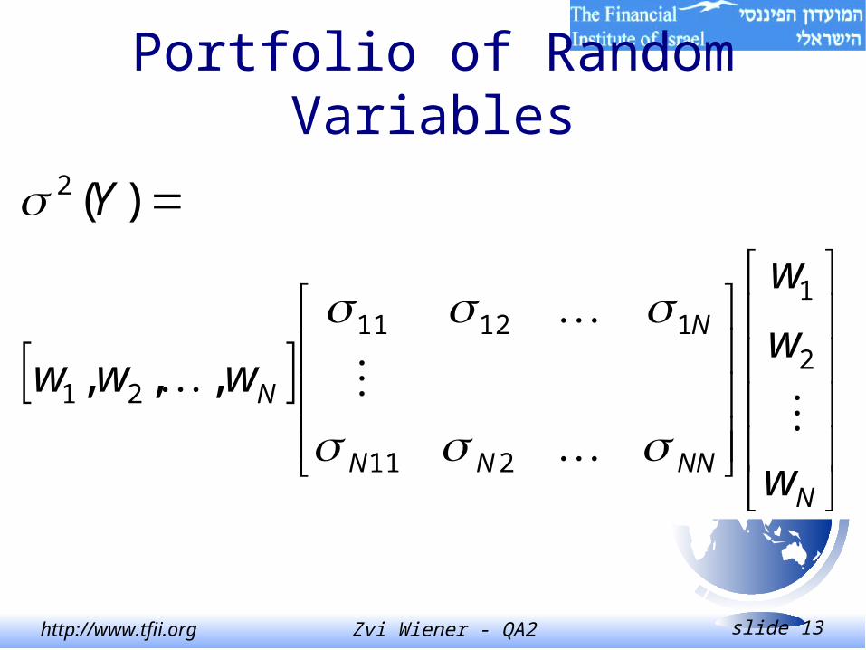
Portfolio of Random Variables

NNNNN

N

N

w

w

w

www

Y

2

1

211

11211

21

2

,,,

)(


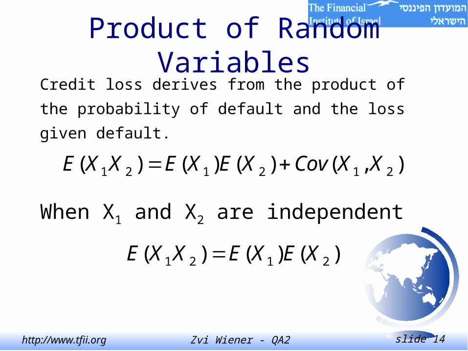
Product of Random Variables

Credit loss derives from the product of the

probability of default and the loss given default.

),()()()( 212121 XXCovXEXEXXE

When X1 and X2 are independent

)()()( 2121 XEXEXXE


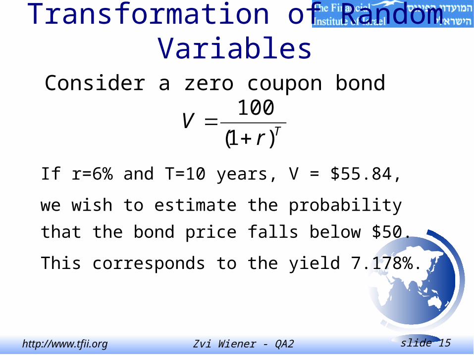
Transformation of Random Variables

Consider a zero coupon bond

TrV

)1(

100

If r=6% and T=10 years, V = $55.84,

we wish to estimate the probability that the

bond price falls below $50.

This corresponds to the yield 7.178%.


The probability of this event can be derived

from the distribution of yields.

Assume that yields change are normally

distributed with mean zero and volatility 0.8%.

Then the probability of this change is 7.06%

Example


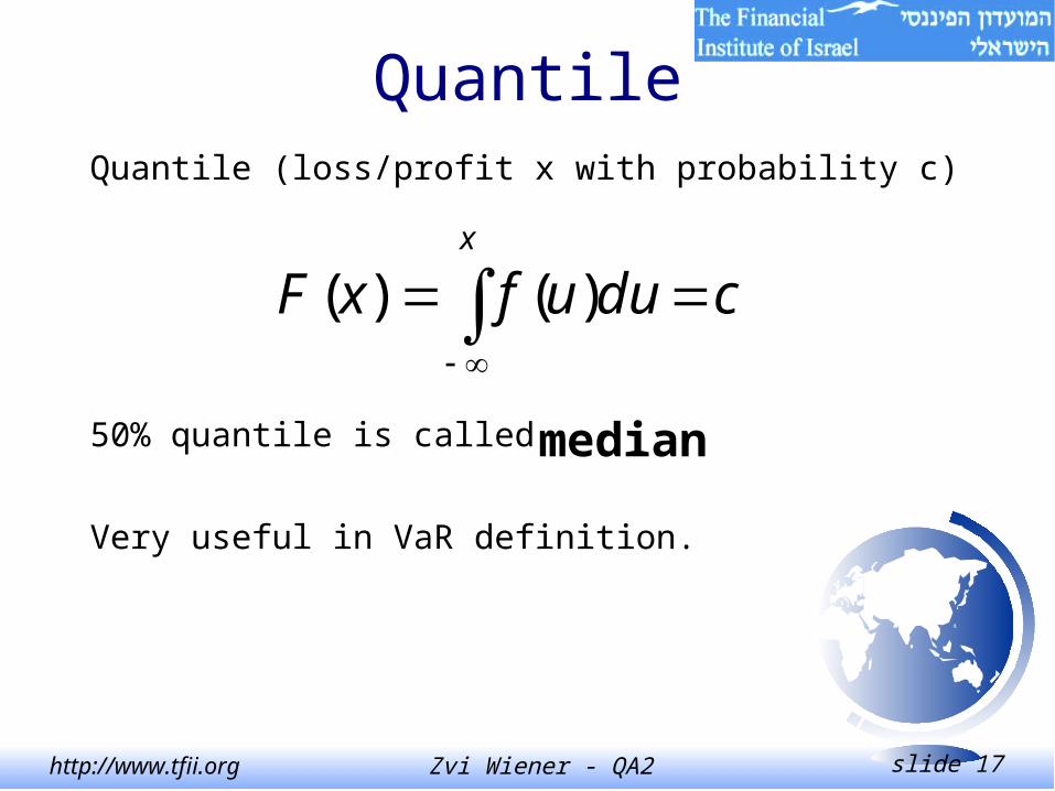
Quantile

Quantile (loss/profit x with probability c)

cduufxFx

)()(

50% quantile is called median

Very useful in VaR definition.


FRM-99, Question 11

X and Y are random variables each of which follows a standard normal distribution with cov(X,Y)=0.4.

What is the variance of (5X+2Y)?

A. 11.0

B. 29.0

C. 29.4

D. 37.0


FRM-99, Question 11

37254.0225 22

BABA 222


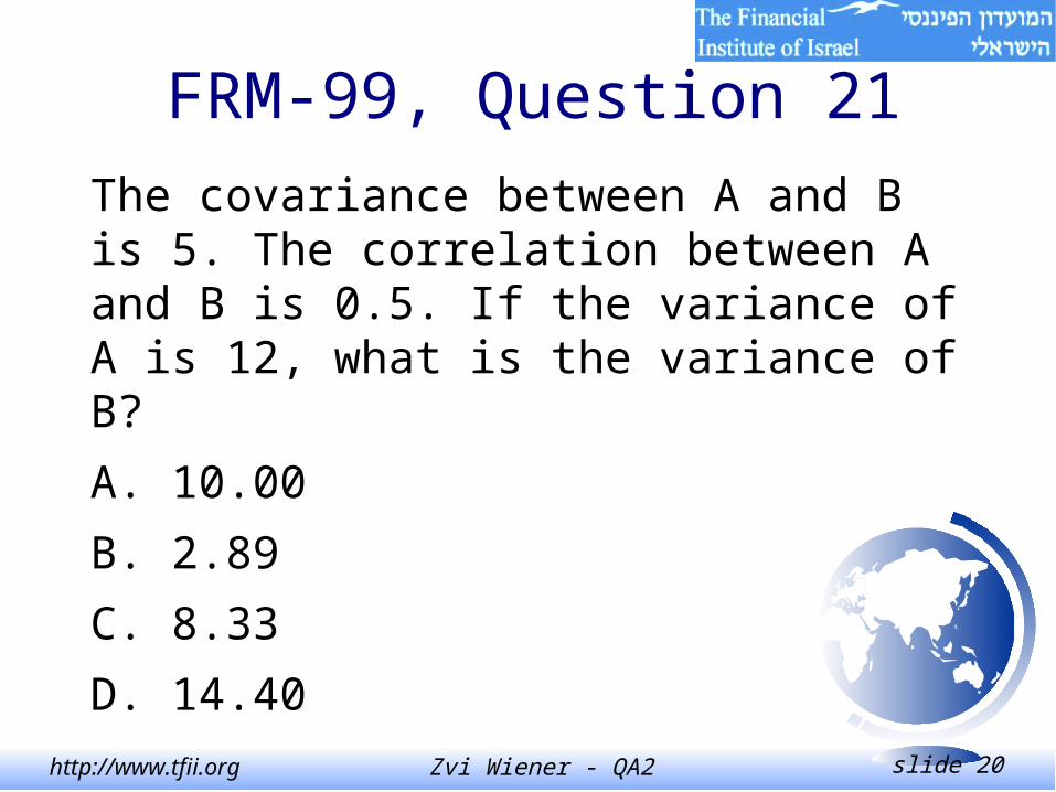
FRM-99, Question 21

The covariance between A and B is 5. The correlation between A and B is 0.5. If the variance of A is 12, what is the variance of B?

A. 10.00

B. 2.89

C. 8.33

D. 14.40


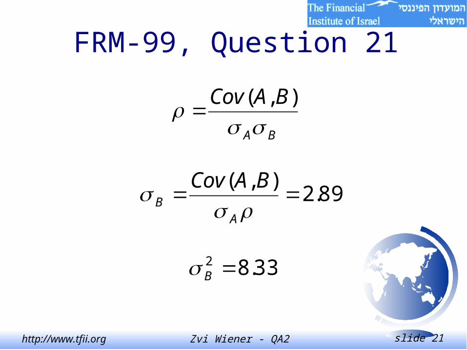
FRM-99, Question 21

BA

BACov

),(

89.2),(

AB

BACov

33.82 B


Uniform DistributionUniform distribution defined over a range of values axb.

bxaab

xf

,1

)(

12

)()(,

2)(

22 ab

Xba

XE

xb

bxaab

ax

ax

xF

,1

,

,0

)(


Uniform Distribution

a b

ab 1

1


Normal DistributionIs defined by its mean and variance.

2

2

2

)(

2

1)(

x

exf

22 )(,)( XXE

Cumulative is denoted by N(x).


-3 -2 -1 1 2 3

0.1

0.2

0.3

0.4

Normal Distribution66% of events liebetween -1 and 1

95% of events liebetween -2 and 2


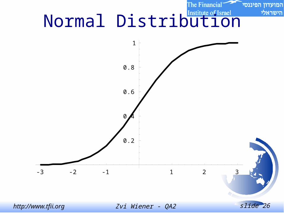
Normal Distribution

-3 -2 -1 1 2 3

0.2

0.4

0.6

0.8

1


Normal Distribution• symmetric around the mean

• mean = median

• skewness = 0

• kurtosis = 3

• linear combination of normal is normal

99.99 99.90 99 97.72 97.5 95 90 84.13 50

3.715 3.09 2.326 2.000 1.96 1.645 1.282 1 0


Central Limit Theorem

The mean of n independent and identically distributed variables converges to a normal distribution as n increases.

n

iiX

nX

1

1

nNX

2

,


Lognormal DistributionThe normal distribution is often used for rate of return.

Y is lognormally distributed if X=lnY is normally distributed. No negative values!

2

2

2

))(ln(

2

1)(

x

ex

xf

22

2

22222 )(,)(

eeXeXE

222 )(ln)(,)(ln)( XYXEYE


Lognormal DistributionIf r is the expected value of the lognormal variable X, the mean of the associated normal variable is r-0.52.

0.5 1 1.5 2 2.5 3

0.1

0.2

0.3

0.4

0.5

0.6


Student t DistributionArises in hypothesis testing, as it describes the distribution of the ratio of the estimated coefficient to its standard error. k - degrees of freedom.

2

12

1

11

2

2

1

)(

k

k

xkk

k

xf

0

1)( dxexk xk


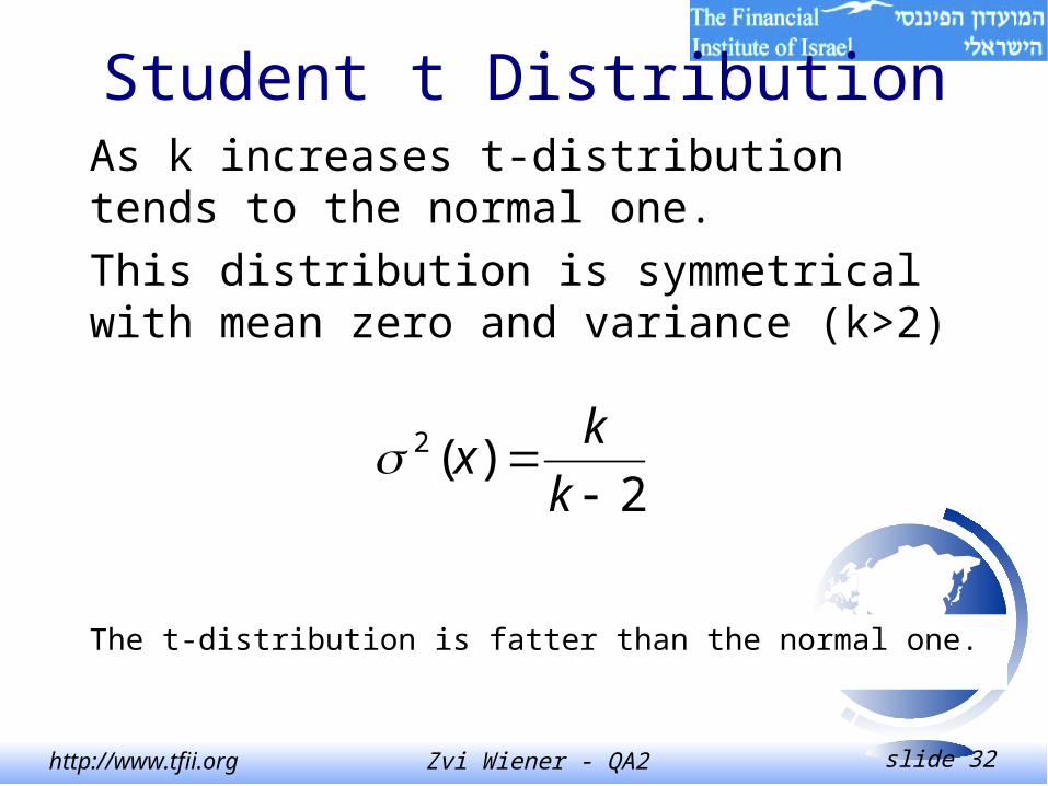
Student t DistributionAs k increases t-distribution tends to the normal one.

This distribution is symmetrical with mean zero and variance (k>2)

2)(2

k

kx

The t-distribution is fatter than the normal one.


Binomial DistributionDiscrete random variable with density function:

nxppx

nxf xnx ,,.1,0,)1()(

nppXpnXE )1()(,)( 2

For large n it can be approximated by a normal.

)1,0(~)1(

Nnpp

pnxz


FRM-99, Question 12

For a standard normal distribution, what is the approximate area under the cumulative distribution function between the values -1 and 1?

A. 50%

B. 66%

C. 75%

D. 95%

Error!


FRM-99, Question 13

What is the kurtosis of a normal distribution?

A. 0

B. can not be determined, since it depends on the variance of the particular normal distribution.

C. 2

D. 3


FRM-99, Question 16

If a distribution with the same variance as a normal distribution has kurtosis greater than 3, which of the following is TRUE?

A. It has fatter tails than normal distribution

B. It has thinner tails than normal distribution

C. It has the same tail fatness as normal

D. can not be determined from the information provided


FRM-99, Question 5

Which of the following statements best characterizes the relationship between normal and lognormal distributions?A. The lognormal distribution is logarithm of the normal distribution.B. If ln(X) is lognormally distributed, then X is normally distributed.C. If X is lognormally distributed, then ln(X) is normally distributed.D. The two distributions have nothing in common


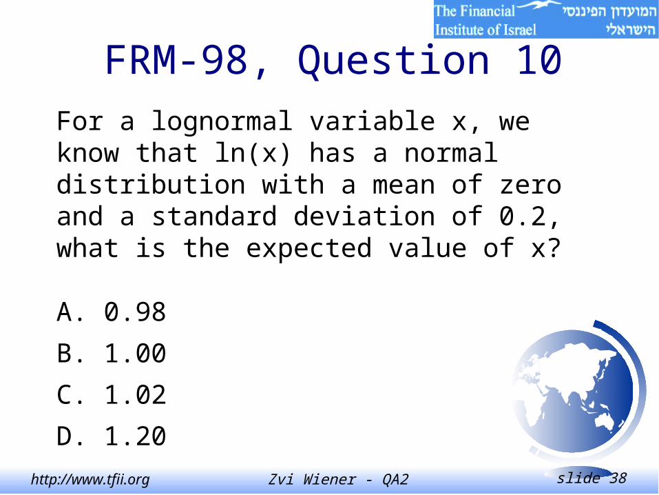
FRM-98, Question 10

For a lognormal variable x, we know that ln(x) has a normal distribution with a mean of zero and a standard deviation of 0.2, what is the expected value of x?

A. 0.98

B. 1.00

C. 1.02

D. 1.20


FRM-98, Question 10

02.1][ 2

2.00

2

22

eeXE


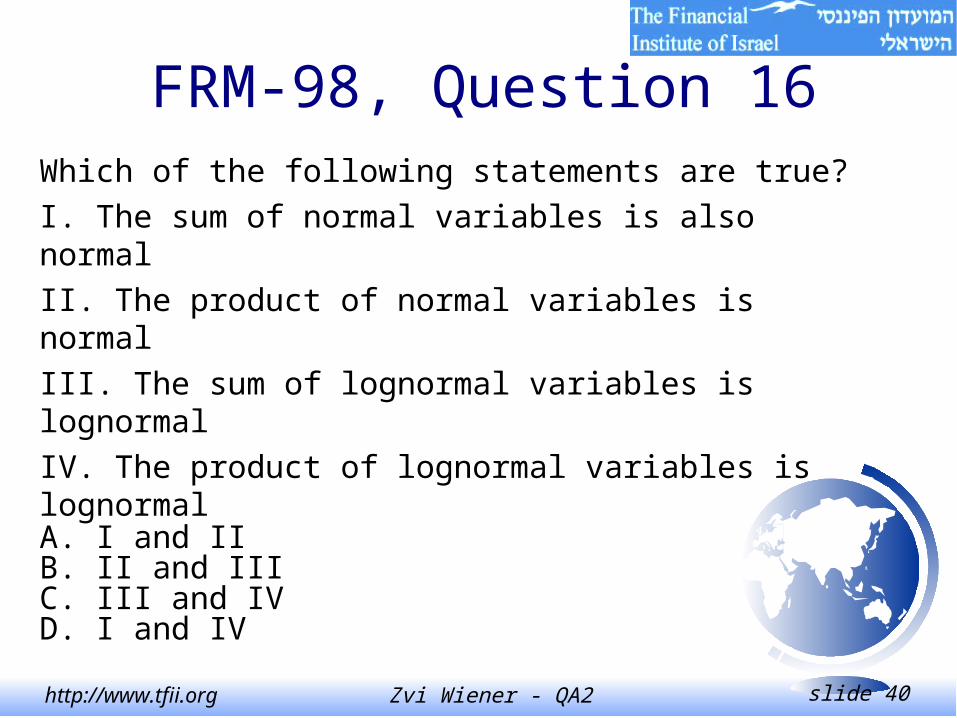
FRM-98, Question 16

Which of the following statements are true?

I. The sum of normal variables is also normal

II. The product of normal variables is normal

III. The sum of lognormal variables is lognormal

IV. The product of lognormal variables is lognormalA. I and IIB. II and IIIC. III and IVD. I and IV


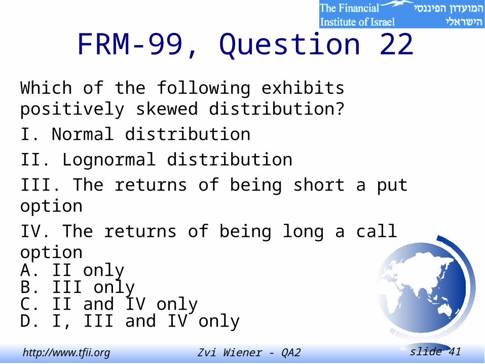
FRM-99, Question 22

Which of the following exhibits positively skewed distribution?

I. Normal distribution

II. Lognormal distribution

III. The returns of being short a put option

IV. The returns of being long a call optionA. II onlyB. III onlyC. II and IV onlyD. I, III and IV only


FRM-99, Question 22

C. The lognormal distribution has a long right

tail, since the left tail is cut off at zero. Long

positions in options have limited downsize,

but large potential upside, hence a positive

skewness.


FRM-99, Question 3

It is often said that distributions of returns from financial instruments are leptokurtotic. For such distributions, which of the following comparisons with a normal distribution of the same mean and variance MUST hold?A. The skew of the leptokurtotic distribution is greaterB. The kurtosis of the leptokurtotic distribution is greaterC. The skew of the leptokurtotic distribution is smallerD. The kurtosis of the leptokurtotic distribution is smaller

qa-2 frm-garp sep-2001 zvi wiener 02-588-3049 mswiener/zvi.html quantitative analysis 2

Documents