LinköpingUniversity|DepartmentofComputerandInformationScienceMasterthesis|StatisticsandDataMiningSpring2017|LIU-IDA/STAT-A--17/008—SE

Channelattributionmodellingusingclickstreamdatafromanonlinestore

KevinNeville

Tutor,OlegSysoevExaminator,BertilWegmann

Upphovsrätt

Detta dokument hålls tillgängligt på Internet – eller dess framtida ersättare – från publiceringsdatum under förutsättning att inga extraordinära omständigheter uppstår.

Tillgång till dokumentet innebär tillstånd för var och en att läsa, ladda ner, skriva ut enstaka kopior för enskilt bruk och att använda det oförändrat för ickekommersiell forskning och för undervisning. Överföring av upphovsrätten vid en senare tidpunkt kan inte upphäva detta tillstånd. All annan användning av dokumentet kräver upphovsmannens medgivande. För att garantera äktheten, säkerheten och tillgängligheten finns lösningar av teknisk och administrativ art.

Upphovsmannens ideella rätt innefattar rätt att bli nämnd som upphovsman i den omfattning som god sed kräver vid användning av dokumentet på ovan beskrivna sätt samt skydd mot att dokumentet ändras eller presenteras i sådan form eller i sådant sammanhang som är kränkande för upphovsmannens litterära eller konstnärliga anseende eller egenart.

För ytterligare information om Linköping University Electronic Press se förlagets hemsida http://www.ep.liu.se/.

Copyright

The publishers will keep this document online on the Internet – or its possible replacement – from the date of publication barring exceptional circumstances.

The online availability of the document implies permanent permission for anyone to read, to download, or to print out single copies for his/her own use and to use it unchanged for non-commercial research and educational purpose. Subsequent transfers of copyright cannot revoke this permission. All other uses of the document are conditional upon the consent of the copyright owner. The publisher has taken technical and administrative measures to assure authenticity, security and accessibility.

According to intellectual property law the author has the right to be mentioned when his/her work is accessed as described above and to be protected against infringement.

For additional information about the Linköping University Electronic Press and its procedures for publication and for assurance of document integrity, please refer to its www home page: http://www.ep.liu.se/.

© Kevin Neville

i

Abstract In marketing, behaviour of users is analysed in order to discover which channels

(for instance TV, Social media etc.) are important for increasing the user’s

intention to buy a product. The search for better channel attribution models than

the common last-click model is of major concern for the industry of marketing.

In this thesis, a probabilistic model for channel attribution has been developed,

and this model is demonstrated to be more data-driven than the conventional last-

click model. The modelling includes an attempt to include the time aspect in the

modelling which have not been done in previous research. Our model is based

on studying different sequence length and computing conditional probabilities of

conversion by using logistic regression models. A clickstream dataset from an

online store was analysed using the proposed model. This thesis has revealed

proof of that the last-click model is not optimal for conducting these kinds of

analyses.

Keywords: Clickstream data, channel attribution, logistic regression, variable

selection, data driven marketing.

ii

iii

Acknowledgements

I would like to thank all my colleagues at Kaplan for providing me with the

objectives and data. Especially I would like to thank Ann-Charlotte Hellström,

Martin Bernhardsson and Victor Wattin for your guidance and inputs and Lovisa

Modin for your mentoring.

My supervisor Oleg Sysoev deserves a huge “spasibo” for keeping my head

above the water during difficult times and always kept me going. Caroline Svahn

did an outstanding job as an opponent. Her work has really had a major impact

on the final thesis. Words cannot describe the help you have given me.

Most importantly I would like to show my gratitude to my adorable girlfriend

Hanna Lundberg for putting up with all this statistics nerdyness during the last

five years. William Luxenburg also deserves some love, thank you for being by

my side and encouraging me to study all night long.

iv

1

Table of contents 1 Introduction ............................................................................................................ 3

1.1 Kaplan ............................................................................................................ 31.2 Background .................................................................................................... 31.3 Related work .................................................................................................. 51.4 Objective ........................................................................................................ 7

2 Data ........................................................................................................................ 82.1 Clickstream .................................................................................................... 82.2 Data summary ................................................................................................ 82.3 Data pre-processing ..................................................................................... 13

3 Methods................................................................................................................ 173.1 Current methods ........................................................................................... 17

3.1.1 Last Click ............................................................................................. 173.2 Probabilistic approach .................................................................................. 18

3.2.1 Attribution formula .............................................................................. 183.2.2 Logistic regression ............................................................................... 20

3.3 Variable Selection ........................................................................................ 223.3.1 Variable elimination techniques .......................................................... 22

3.4 Bootstrap method ......................................................................................... 233.5 Random forest .............................................................................................. 23

4 Results .................................................................................................................. 254.1 Last-click model ........................................................................................... 254.2 Logistic regression with single channels ..................................................... 264.3 Attribution formula without using variable selection .................................. 274.4 Attribution formula when using variable selection ...................................... 29

5 Conclusions .......................................................................................................... 326 Discussion ............................................................................................................ 338 Literature .............................................................................................................. 369 Appendix .............................................................................................................. 38

9.1 Model 1 ........................................................................................................ 389.2 Model 2 ........................................................................................................ 399.3 Model 1 after stepAIC ................................................................................. 409.4 Model 2 after stepAIC ................................................................................. 41

2

List of figures Figure 1. Example of a customer journey. .............................................................. 4Figure 2. Web traffic per minute. ............................................................................ 10Figure 3. Histogram of window measurement. ..................................................... 11Figure 4. Histogram of gap measurement. ........................................................... 12Figure 5. Example of data before separation. ...................................................... 13Figure 6. Example of data after separation. .......................................................... 14Figure 7. Histogram of time between events where constant T is marked. ..... 15Figure 8. Example of sequence creation. .............................................................. 16Figure 9. Variable importance plots of attribution model without variable

selection. ............................................................................................................. 27Figure 10. Result of attribution model with bootstrapping and without variable

selection. ............................................................................................................. 28Figure 11. Variable importance plot of attribution model with variable

selection. ............................................................................................................. 29Figure 12. Result of bootstrapping with variable selection. ................................ 30 List of tables Table 1. Variable description. .................................................................................... 9Table 2. Channel description. ................................................................................... 9Table 3. Share of channels. ..................................................................................... 10Table 4. Data summary statistics. .......................................................................... 11Table 5. Frequency of steps by customer journey. .............................................. 12Table 6. Example of D1. ........................................................................................... 17Table 7. Example of D2. ........................................................................................... 17Table 8. Last click attribution. .................................................................................. 25Table 9. Result of logistic regression using single channels. ............................. 26Table 10. Result of attribution formula without variable selection. .................... 27Table 11. Result of attribution formula with variable selection. ......................... 29Table 12. 95% Confidence interval of Bootstrapping result. .............................. 30

3

1 Introduction

1.1 Kaplan This thesis work was done in cooperation with Kaplan that provided data for the

analyses and helped with specifying the objectives. Kaplan is a customer and

loyalty management firm which consults their clients in their marketing

strategies. Kaplan focus on Customer relationship management (CRM) and

offers solutions for the entire CRM process, including technical, strategic,

analytical and creative solutions (Kaplan Loyalty Management, 2017). In Ryan

(2017), the CRM process is described as the practice of understanding the

customers desire and maintaining a personal relationship with each customer.

1.2 Background Modern marketing uses data analysis to understand the needs and desires of the

customer. Ryan (2017) mentions Digital Marketing as a concept to describe this

new era in marketing. Recent studies predict the internet usage and the number

of internet connected devices per person to increase rapidly in the near future

(Internetstiftelsen Sverige, 2016; Business Insider Inc, 2016). Therefore, digital

marketing could be even more important in the future than today. Digital

marketing belongs to one of the largest expenses in a company’s marketing

budgets. However, there are no good ways to evaluate the performance of these

investments (Lemos, 2015; Ryan, 2017).

Kotler and Armstrong (2013) explain The Buyer Decision Process as a journey

through different psychological stages before customers decide to buy a product

or not. A customer’s journey is expressed by Ryan (2017) as a chain of events

affecting a customer when buying a product. This concept is strongly connected

to Attribution, which is the process to identify how much each event in a

customer journey contribute to the desired outcome (Ryan, 2017).

A typical e-commerce store advertises themselves using different medias, these

are referred to as different Channels Zhang et al. (2014). The purpose of the

channels is to refer customers to visit the e-commerce store. The channels are

4

divided into offline channels as TV commercials or online channels as social

media, email, search engines or other websites (Ryan, 2017). Channel attribution

is defined as the process of measuring how these channels contribute to a

customer reaching conversion, the desired outcome. A typical example of a

conversion state is when the customer buys the product being advertised. Once

a customer has entered the e-commerce store, a new session begins. If this

session does not end in conversion, then it is noted as Null. Figure 1 illustrate an

example of a customer journey.

Figure 1. Example of a customer journey. The example illustrated in Figure 1 ended in conversion at visit 3 and the

customer was referred to the website by the channels social media and email.

Simple rule based methods are widely applied in the industry to estimate the

channel attribution. These models are not derived from the actual data, instead

they are pre-determined rules originated from expert opinions deciding the

resulting attribution (Shao and Li, 2011). Dalessandro et al. (2012) mention

how the need for more efficient models for channel attribution is of great

concern for marketers. This is also noted in Zhang et al. (2014) to be a trend in

research. The subject is interesting since it affects many businesses and would

t=1 t=3 t=2

Session3:..ClicksinsidetheOnlinestore..Conversion

Session2:..ClicksinsidetheOnlinestore..Null

Session1:..ClicksinsidetheOnlinestore..Null

Visit2.Channel:Socialmedia.

Visit3.Channel:Email.

Visit1.Channel:Socialmedia.

5

enable them to optimize the allocation of their spending on marketing (Ryan,

2017).

Dalessandro et al. (2012) propose three properties which a good attribution

model should have:

1. Fairness: the model should acknowledge each channel according to its

ability to divert the customer to conversion.

2. Data driven: the attribution model should be derived from data, not from

doubtful opinions about the industry in general.

3. Interpretability: the model should be applicable in industry and output

an understanding of how channels perform.

Clickstream is defined as a database storing journeys of customers. Clickstream

data can be generated by both web services and mobile apps. The information

about a user’s behaviour on a website is stored in web log files which makes this

information hard to use for computations of channel attribution. A clickstream

can be difficult to analyse since the data can be in an unstructured format. In this

thesis, we propose a strategy for restructuring of the log data into a format which

is easy to process by channel attribution models.

1.3 Related work Today’s methods for channel attribution consist of simple rule based methods

such as First- and Last Click, Time Decay and Equal Weight among others

(Ryan, 2017). Shao and Li (2011) state the last click model to be the most

common attribution model in the industry. According to Jayawardane et al.

(2015), the last click model is often used as a benchmark model in research.

These methods are often used because of their simplicity. However, these

methods have some drawbacks: customers tend to have longer patterns than just

one click, which the rule based methods do not take into consideration.

Moreover, these models are not based on the actual data, but rather on expert

opinions which cannot always be justified (Ryan, 2017).

6

Development of better attribution models is a research direction that recently

attracted much attention. Shao and Li (2011) are often referred to as the first

researchers to propose a more sophisticated model which would credit multiple

channels for each conversion (Abhishek et al. 2012; Dalessandro et al. 2012).

These authors propose two models to tackle the problem of channel attribution

modelling. One of their models is a Bagged Logistic Regression (Anderl, Becker,

von Wangenheim, & Schumann, 2016), in which bagging is used in order to

reduce estimation variability due to high correlation in the covariates. Both

observations and covariates are being sampled in each iteration. Another

proposed model is a simple probabilistic model where they compute the

probabilities of positive user interaction in each channel. A positive user is a user

who committed a purchase. The authors extend this model to a second-order

model where these probabilities are calculated pairwise for between channels.

The probabilities are summed for a respective channel to represent the attribution

of each channel. The authors mention difficulties for higher order models due to

difficulties finding third order interactions. Therefore, the second order model

was used. The logistic model received a lower misclassification rate but higher

variance, the result was the opposite in the probabilistic model. Their paper

resulted in implementing the probabilistic model in a real business situation

(Shao and Li, 2011).

Anderl et al. (2016) propose to represent the customer’s journeys as chains in

directed Markov graphs. Each channel is represented as a state. Three additional

states are included in the model. Start, Conversion and NULL. These states

represent the start of the journey, a positive conversion and negative conversions

respectively. The transition probability corresponds to the probability of

connection in channel “i” followed by a connection in channel “j”. To measure

the effect of each channel, the authors use the concept of removal effect; the

probability of reaching the conversion state from the start state when channel “i”

is removed. The authors claim this to be an effective way of measuring the

contribution of each channel (Anderl et al. 2013).

7

A hidden markov model approach is used as an attribution model in Abhishek et

al. (2012). Their approach is inspired by the theories behind the conversion

funnel. The conversion funnel is a well-established concept in marketing, first

introduced by Elmo Lewis (Barry, 1987). It is a theoretical mapping of the stages

of customer journeys. The model proposed by Abhishek et al. (2012) consists of

four states; Disengaged, Active, Engaged and Conversion, which represents the

psychological state the user associate with in the conversion funnel. The authors

investigate how customers behave when seeing various ads in different channels.

Their conclusion is that the display ads are the most efficient tool in the early

stage of the conversion process and search ads perform well across all stages.

1.4 Objective The objective of this thesis is to develop probabilistically motivated and data

driven models for channel attribution by using clickstream data and then

study how these models are related to existing channel attribution

models. More specifically, this thesis is focused on the following research questions:

• What variables in clickstream data are relevant for modelling channel

attribution?

• How can the clickstream data be used to construct a probabilistic model

for channel attribution?

• Is the common method “last-click” good enough compared to more

advanced models for modelling channel attribution?

8

2 Data Data from a specific Kaplan client are used in this thesis. The client is a

sportswear online store with customers from a variety of countries. The data is

given in the form of a clickstream, which contains all the clicks that have been

made on the site and the referring channel for each session. In its raw format, the

clickstream consists of over 600 variables and millions of rows. However, to

address the research questions of this thesis, we only need variables containing

the information about how customers entered the website and what made

customers enter the online store. Therefore, many variables and the rows

representing the internal clicks (i.e. clicks within the same session) can be

excluded. However, the internal clicks contain information whether the session

resulted in a conversion or not. This will be handled in the pre-processing of the

data.

The dataset is extracted between 2016-11-06 to 2016-12-31 which was chosen

by the commissioner Kaplan since the client executed televised campaigns and

several online campaigns during this period, also called the “Black weekend”.

2.1 Clickstream A fundamental part of the clickstream data is the ability to track users. A

clickstream does this by using Cookies. A cookie in an online context is a file

stored locally on each user’s device and contains information about the browsing

behaviour for a specific device. This cookie allows the weblogs to follow a user

over time which makes the clickstream a suitable source to measure attribution.

Clickstreams have previously been used to cluster customers based on their

previous behaviour. Alswiti et al. (2016) used a clickstream to identify users and

classified them as a normal user and a malicious user. In another paper,

clickstreams were used to cluster users and then handle them differently

depending on how they act and navigates on the website (Lu et al., 2013).

2.2 Data summary It is required to transform the data set in order to make it useful for analysis. This

chapter will first give a summary of what variables the dataset consists of, some

9

basic statistics and lastly how the transformations and manipulations of data has

been performed.

Four variables are kept from the clickstream; ID, Time, Channel and Conversion.

Table 1 describes each variable in the data.

Table 1. Variable description. Variable Description Type ID Unique ID for the customer journey Label Time Denotes at what time the visit started. Date, yyyy-mm-dd hh:mm:ss

Channel Denotes which channel that was being used to enter the online store.

Categorical

Conversion 1 = If the visit reached conversion, 0 otherwise.

Binary

The raw data consist of 31 different channels. In this thesis, the channels are

grouped into six different groups by merging channels of similar kind into one

group. This reduces complexity for the models and gives a more general

interpretation of different types of channels. The final six channels are described

in Table 2.

Table 2. Channel description. No. Channel Description 1 Email The user reached the online store by a link in an email. 2 Other The user reached the online store by any other website, such as a blog. 3 Search The user reached the online store by a search engine. 4 Social The user reached the online store by either Facebook, LinkedIn,

Instagram, Twitter or YouTube. 5 TV The user reached the online store by a search engine while a television

commercial was broadcast. 6 Website The user reached the online store by typing its URL address directly in

the web browser.

Televised ads do not have a tracking system as with the cookie solution (Kitts et

al., 2010). A visitor's channel will be classified as TV if the visit occurred within

the interval of 5 minutes before the advertisement and 20 minutes after the start

of the advertisement, while the original channel was Search. This interval is

created since the scheduled time for the televised ad is approximate. The range

of the interval is chosen by expertise opinions at Kaplan.

At what time the visits and television advertisements occured are visualized in

Figure 2.

10

Figure 2. Web traffic per minute.

The light red area indicates when the Black weekend occurred, which is a recent

phenomenon in Sweden. Many retailers use this period to give valuable offers

before the Christmas shopping begins in December. The orange lines indicate

the period of a televised ad. One can see that the traffic peaks around these

televised commercials, with its major peak on Boxing day.

The share of each channel in the data can be seen in Table 3.

Table 3. Share of channels. Search Website Social Email TV Other

0,409 0,327 0,194 0,039 0,017 0,014

Search is the most common channel and Other the least common channel.

Some basic statistics of the data are given in Table 4. Some important measures

are:

11

• Gap = Time between two adjacent events within a journey.

• Window = Time between the first and last event of a journey.

• Steps = Number of visits per journey.

Table 4. Data summary statistics.

Number of visitors 153916

Number of visits 181045

Mean steps 1.18

Mean gapTime (in days) 4.89

mean windowTime (in days) 9.20

Journey conversion rate1 0.0306

The time aspect can be further investigated using histograms to investigate the

distribution of the window and gap measurements. Here the journeys with only

one step is excluded since their distance (Gap and Window) is always zero and

therefore they would skew the histograms towards left.

Figure 3. Histogram of window measurement.

1 Number of journeys ending in conversion divided by number of journeys.

12

Figure 4. Histogram of gap measurement. Both histograms show a similar pattern where most observations lie between

zero to five days. One difference in the histograms is that the window histogram

has much longer tail than the gap histogram. Also, the frequencies of the

journeys’ lengths need to be investigated. The result can be found in Table 5.

Table 5. Frequency of steps by customer journey. Steps Frequency

1 139484

2 9696

3 2454

4 980

5 485

6 256

7 146

8 111

9 64

>10 240

13

One can see that the majority of journeys is only one step long and the frequency

is quickly decaying as the steps increase.

2.3 Data pre-processing The data are censored in time both from the left and from the right since data is

extracted for a specific period of time. This causes difficulties in knowing when

a customer journey has started and when it ends.

Some journeys contain visits after a conversion has been reached, or it contains

multiple conversions. These types of situations need to be addressed somehow.

To tackle this problem, the journeys will be split into smaller sequences so it can

only contain one conversion per sequence. This will result in that all events

following a conversion will belong to a new sequence. One sequence may consist

of several sub-journeys with different purposes, and therefore they are separated.

Figure 5. Example of data before separation. Figure 5 illustrates the journey of three customers before separation. The result

after separation is illustrated in Figure 6.

14

Figure 6. Example of data after separation. The separation of data results in another take on the analysis; instead of analysing

by user, the analysis will be performed by sequence. Another important problem

is how to define whether a given sequence is complete or if there is only access

to a part of the sequence.

As mentioned earlier this is not clear since the data are censored. The current

data might contain sequences which has not ended yet. Therefore, some data

manipulations are needed to enable a valid input for our models.

Figure 7 is the same as Figure 4, but now with a red line indicating the 95%

quantile, denoted by T.

15

Figure 7. Histogram of time between events where constant T is marked. T will be considered as a threshold value that indicates the completion of the

sequence. The 95% quantile is chosen to represent the majority of the data.

The cut-off point of the data collection will be named TEnd, this represents the

time when the data starts being censored to the right.

More specifically, T will then be used as follows:

1. If the difference in time between two adjacent steps in one sequence is

larger than T, the sequence will be considered to have ended and therefore

the second step will be the start of the next sequence in the journey.

2. If the difference in time between the last step in a sequence and TEnd is

larger than T, then it will be said to have ended and thereby given the state

Null.

3. If the difference between the last step in a sequence and TEnd is smaller

than T, this sequence is said to still be unfinished and we believe this

sequence will continue after the cut-off point of the data collection.

16

After all journeys have been processed in accordance with the criteria specified

above, we can split the journeys into sequences. These sequences can either end

in conversion, end with Null or still be unfinished. We filter the data by

discarding the unfinished sequences.

An example of how a journey is processed is visualized in Figure 8.

Figure 8. Example of sequence creation. ID=1 would here be said to still be unfinished since the last step is closer to TEnd

than T, and therefore discarded from further analysis.

ID=2 would here be separated into two sequences since the time difference

between step two and step three have a distance in time greater than T. The

distance in time between step four and TEnd is also larger than T, thus, the second

sequence will also end with Null if the last step did not reach conversion.

ID=3 would here be kept as is. This sequence ends with Null if the last step did

not reach conversion, since the distance in time to TEnd is larger than T.

Two datasets are created after the sequences has been transformed with respect

to T and TEnd. The datasets will be in a binary format and represent the channels

present in each sequence. The ordering can be seen in the interaction columns

(see the fifth and sixth column in Table 7). The first part of an interaction column

17

represents the second-to-the last step in the sequence. The second part represents

the last step in the sequence.

The first dataset, D1, consists only of sequences where the total number of steps

equals to one. D1 does, therefore, not have any interaction columns. The

sequences in Figure 5 would be represented as Table 6 if sequence two in Figure

5 would end in conversion and sequence one and three in Figure 5 would end in

the state Null.

Table 6. Example of D1. ID Conversion Channel1 Channel2 Channel3 Channel4 Channel51 0 0 0 1 0 02 1 0 0 0 1 03 0 0 0 0 0 1

The second dataset, D2, consists of all sequences with at least two steps.

However, only the last two steps per sequence will be considered in D2. This to

reduce complexity as it is concluded to be sufficient for answering the objectives

of the thesis.

Table 7. Example of D2. ID Conversion Channel1 Channel2 Channel2,Channel1 Channel1,Channel21 0 1 0 1 02 1 0 1 0 13 0 0 1 0 1

Each row in D1 and D2 represents one sequence. The columns consist of an ID,

the y-variable Conversion and all the channels. A “1” in the Conversion column

indicates the sequence ended in Conversion, “0” otherwise. A “1” in the channel

columns indicates this specific channels to be present in the sequence.

3 Methods

3.1 Current methods

3.1.1 Last Click The most common method today is the Last Click model. This method assigns

all attribution to the last channel before conversion (Ryan, 2017).

18

Last click algorithm:

1. For each channel: sum the number of occasions when the channel was

present in the last step before conversion.

2. Divide each sum by the total number of conversions to obtain each

channel attribution in percentages.

This approach contradicts the properties described by Dalessandro et al. (2012)

of a suitable attribution model since it will not yield a fair estimation of each

channel’s attribution. The limitations of the last click attribution approach call

for more rigorous and scientifically motivated methods that would be able to use

the observed data in an efficient way.

3.2 Probabilistic approach We propose a new attribution model that is probabilistically motivated and data

driven to a larger extent than the last click model. Our attribution model will

consider the ordering and time between visits; time will be important in the

creation of the sequences and the ordering will explicitly be used in the

attribution model. This approach will be the first of its kind that uses the time

aspect in the computations of the channel attribution.

3.2.1 Attribution formula In statistical terms, the attribution problem can be formulated as follows.

!""#$%&"$'( )* = , )'(-.#/$'( 12 = )*'#12-4 = )*) ( 1 ) where )* represent a channel from the available set of channels, Sn is the notation

for the last step, and Sn-1 denotes the second-to-last step. We denote:

6 = )'(-.#/$'(

7 = {12 = )*'#1294 = )*}

; =1,23,,$@1A = 1$@1A ≥ 2,$@1A ≥ 2,

12 = )*1294 = )*

19

where SL is the sequence length. Obviously, Z= {1,2,3} covers all possible

outcomes. By using conditional probability definition, we get:

, 6 7 = C(E|G)C(G)

= C(E,G,HIHJ)C(G)

K*I4 =

=C 6 7, ; = ;* ∙C G,HIHJ

MJNO

C G= COPCQPCM

CR ( 2 )

Since {12 = )*'#1294 = )*} and {1A ≥ 2, 12 ≠ )*} leads to

{1294 = )*, 1A ≥ 2}, we get the following expressions for P1, P2, P3 and P4:

,1 = , )'(-.#/$'( )2 = )*, 1A = 1)*,()2 = )*, 1A = 1) ( 3 ) ,2 = , )'(-.#/$'( )2 = )*, )2-4 = )U, 1A ≥ 2)*,()2 = )*, )2-4 = )U, 1A ≥ 2)U ( 4)

,3 = , )'(-.#/$'( )2 = )U, )2-4 = )*, 1A ≥ 2)*,()2 = )U, )2-4 = )*, 1A ≥ 2)U ( 5 ) The sum of the probabilities P1, P2 and P3 will then be divided by P4 as stated in

Equation 2.

,4 =P(12 = )*'#12-4 = )*) ( 6 )

This will return a probability of reaching conversion for each channel where all

possible outcomes have been concerned. Logistic regression is used to estimate

, )'(-.#/$'( )2 = )*, 1A = 1) ( 7 ) in Equation 3,

, )'(-.#/$'( )2 = )*, )2-4 = )U, 1A ≥ 2) ( 8 ) in Equation 4 and

, )'(-.#/$'( )2 = )U, )2-4 = )*, 1A ≥ 2) ( 9 ) in Equation 5. The logistic model will be explained in more detail in the next

subsection.

20

3.2.2 Logistic regression Logistic regression is a common method used in many scenarios. Logistic

regression is believed to be the most common model that is being used to fit

dependence between a set of predictors and binary outcome (Hastie et al., 2009).

We will use it to obtain the probabilities of conversion in P1, P2 and P3 of

Equation 3,4 and 5.

Hosmer et al. (2013) mention two important reasons for choosing logistic

regression. They claim logistic regression to be a flexible and easily used

function. Shao and Li (2011) agree logistic regression being flexible and claim

it outputs interpretable findings. The literature also mentions the logistic

regression to be stable and work well even though collinearity is present.

Hosmer et al. (2013) explain linear regression as the representation of the

conditional mean of response Y given input vector x as

W X = Y(7|X). ( 10 )

The probability of conversion (Z) is then given by the formula for the logistic

regression which is defined as:

W X = [\]^\O_

4P[\]^\O_. ( 11 )

The log-odds of Equation 11 will result in:

g x = ln e(U)

4-e(U)= fg + f4X ( 12 )

In our attribution model, the input variables will be binary and represent the

channel columns in D1 and D2 respectively. Equation 11 and 12 can be expanded

as follows. We denote a vector x´=(x1, x2, … xp) to represent whether the

21

sequence contains the given channels or combinations of channels or not. Thus,

the logistic multiple logistic regression is written as follows:

g x = ln e(U)

4-e(U)= fg + f4X4 + fiXi + ⋯fkXk ( 13 )

where the multiple logistic regression model is given by

W X = [l(_)

4P[l(_) ( 14 )

The probability in Equation 7 will be estimated by fitting a Logistic regression

using the D1 dataset. These coefficients will then be used to obtain W X in

Equation 14.

Equation 8 and 9 will be estimated by fitting a logistic regression using dataset

D2 and then used to obtain the probability using Equation 14.

The models will then be used to obtain the probabilities of all possible outcomes

for the respective models as explained in Equation 7, 8 and 9.

It is common to estimate the beta parameters using maximum likelihood. We

will use the R-package “glmnet” to estimate the logistic regressions. The

“glmnet” package use an iterative updating process, Iteratively Reweighted Least

Squares (IRLS) to obtain the parameters (Friedman et al, 2010; Hastie et al,

2009).

22

3.3 Variable Selection Overfitting might occur when the model complexity is too high for the given

data. This is common when there are many explanatory variables. A common

technique of reducing overfitting is to use some shrinkage technique like Lasso

regression or to perform variable selection (Hastie et al., 2009). If variable

selection is used, the final model is normally less complex than the original

model and thus the estimation will not be overfitted to the training data. We use

the following popular method for variable selection.

3.3.1 Variable elimination techniques Testing all possible combinations of variables to estimate a model is time

consuming. Stepwise selection is a technique for selecting a set of variables

without having to go through all possible combinations. We use Stepwise

selection since we want to obtain which combinations of channels to explain

conversion rather than shrink all coefficients. Based on Akaike's information

criterion (AIC) it is possible to obtain a subset of variables to use in the logistic

regression models. The set of variables that receive the lowest AIC score will be

used in the final model.

In the original paper by Akaike (1974) AIC is calculated as follows:

!m) = -2 *n'on$p + 2p, ( 15 )

where k is the number of parameters.

Forward-stepwise selection begins with a model consisting of just an intercept.

In each iteration, the variable which leads to the greatest improvement in AIC is

added to the model. This continues until the AIC does not continue to decrease.

Backward-stepwise selection starts with the full model and remove variables one

at a time to decrease the AIC score in each iteration. The algorithm continues

until it does not improve the AIC anymore (Hastie et al, 2009).

A third option is to use a hybrid between forward- and backward-stepwise

selection. In this case, the model can add or remove variables in each iteration.

23

Backward-stepwise selection can only be used when N>p. Forward-stepwise

selection can always be used but preferred to be used when p >> N. We have

chosen to use the hybrid approach in order to be as flexible as possible.

This is a good method since it penalizes models with many parameters and

models with a poor fit. The result should be an indication of which channels that

are important for explaining conversion (Hastie et al, 2009).

3.4 Bootstrap method Bootstrapping is a resampling method used to determine a statistic by estimating

it several times with different subsets of data (Hastie et al., 2009). We use

bootstrapping to fit our logistic regression models with different samples of data.

Each sample consists of 10 000 observations sampled with replacement. By

using bootstrapping, we create 1000 different samples to fit our models and

thereby estimating each channel attribution 1000 times. This allows a confidence

interval to be calculated for the attribution of each channel.

3.5 Random forest Bagging is a technique that is used to reduce variance in a prediction (Hastie et

al., 2009). With bagging, it is possible to fit a model multiple times to a new

sample from the data. The output of bagging is achieved by averaging the

estimated models’ parameters which yields a model with less variance.

Random forest by Breiman (2001) is an extension to bagging. Breiman states this

is a good technique for prediction, especially for classification. Hastie et al.

(2009), claim that random forests are easily trained and tuned and therefore the

method has become very popular.

Random forest estimates multiple classification trees where a random set of

variables are chosen in each fit. Hastie et al. (2009) give a good explanation of

the algorithm.

24

Random forests can also be used to estimate variable importance, which is how

it will be used in this thesis. The Gini index will be used as splitting criterion.

q$($$(r.X = stu(1 − stu)wuI4 , ( 16 )

where k=class, m=node and s is the share of observations assigned to class k in

each node m. At each split in each tree, the improvement in the split-criterion is

the importance measure attributed to the splitting variable, and is accumulated

over all the trees in the forest separately for each variable (Hastie et al., 2009).

This can be represented by a variable importance plot to investigate which

variables are important for classifying conversion.

Random forest models are not in need of validation techniques such as cross-

validation. Instead, a technique called Out of Bag (OOB) is used. OOB calculates

the average classification for every observation only based by the decision trees

where the observation was not included in the sample data used to estimate the

tree.

25

4 Results In this section, the results of all the models will be presented. Firstly, the rule

based method results will be presented. The last click model will be considered

to be a benchmark model since the last click is the most common method today.

Then the result of the classifier approach will be presented and evaluated.

4.1 Last-click model The order of the channels is of more interest than the actual percentage it has

been given. Table 8 illustrates the result of attribution when using the last-click

model.

Table 8. Last click attribution.

Channel AttributionSearch 0.5035Website 0.3483Email 0.0820Social 0.0429TV 0.0154Other 0.0078

There is a wide gap between the top two channels and the four bottom channels.

Search and Website is clearly the most common last click channels. The result

of the last-click model is similar to the share of channels presented in Table 3,

especially the size ordering of channels.

26

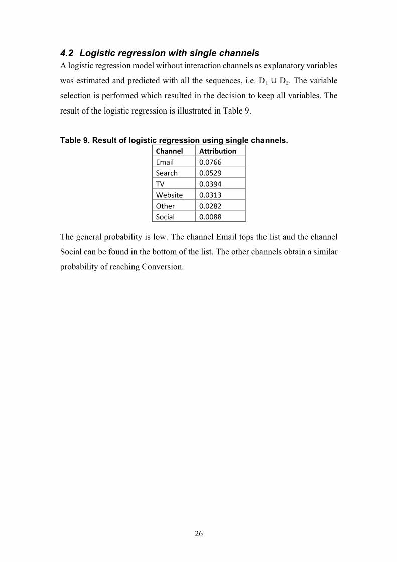
4.2 Logistic regression with single channels A logistic regression model without interaction channels as explanatory variables

was estimated and predicted with all the sequences, i.e. D1 ∪ D2. The variable

selection is performed which resulted in the decision to keep all variables. The

result of the logistic regression is illustrated in Table 9.

Table 9. Result of logistic regression using single channels. Channel AttributionEmail 0.0766Search 0.0529TV 0.0394Website 0.0313Other 0.0282Social 0.0088

The general probability is low. The channel Email tops the list and the channel

Social can be found in the bottom of the list. The other channels obtain a similar

probability of reaching Conversion.

27

4.3 Attribution formula without using variable selection Next is the result from using Equation 3 when no variable selection was

performed. The result is shown in the table below.

Table 10. Result of attribution formula without variable selection. Channel AttributionEmail 0.0678Search 0.0500TV 0.0452Other 0.0324Website 0.0248Social 0.0091

Email tops the list and social can be found in the bottom. The probability is in

general low and evenly distributed among the channels, except for the absolute

top and bottom of the list.

Variable importance was found using random forest.

Figure 9. Variable importance plots of attribution model without variable selection. The y-axes consist of the twenty most important variables and the x-axes

represents the Gini index. The channel Social tops the list and can be found in

the top three combinations in all three plots. The single channels are all present

28

in the plots. However, Search is not present in the second plot and Website is not

present in the last plot.

Figure 10. Result of attribution model with bootstrapping and without variable selection.

The result of Bootstraping is visualized in Figure 12. The x-axis represents the

obtained attribution for the respective channel.

The attribution of the channel Social is the lowest among the channels and Email

has the highest attribution. The other channel attributions are centred around 0.5.

It is challenging to distinguish which channels perform better than other since

many channel distributions overlap. However, Email has a significantly higher

attribution value than Social.

29

4.4 Attribution formula when using variable selection In this result the models used in the attribution formula has been optimized using

variable selection. The subset of variables after performing variable selection is

the same as the full model for P1 in Equation 3.

The logistic regression concerning P2 and P3 discarded some variables as the

variable selection was performed. 16 variables were considered to be enough to

explain Conversion, these can be found in Appendix 9.4. The result of the

attribution model can be found in the Table 11.

Table 11. Result of attribution formula with variable selection.

Channel AttributionEmail 0.0752Search 0.0515TV 0.0457Other 0.0346Website 0.0275Social 0.0093

The ranking of the channels is the same as in Table 10. However, the value of

attribution has increased for all channels.

Figure 11. Variable importance plot of attribution model with variable selection.

Social is clearly considered to be the most important variable for all plots. The

rest of the variables are fairly similar.

30

Figure 12. Result of bootstrapping with variable selection. The distribution of each channel has is more centred in comparison to Figure 10.

Website and Search do not overlap anymore and since Search has a significantly

higher attribution value it can be said to outperform Website.

Table 12. 95% Confidence interval of Bootstrapping result. Mean Lowerbound UpperboundEmail 0.09109 0.06559 0.11660Other 0.03737 0.00489 0.06986Search 0.06010 0.05221 0.06799Social 0.01029 0.00575 0.01482TV 0.0500 0.01896 0.08104Website 0.03569 0.02979 0.04159

Table 12 contains the mean and lower- and upper bound of the 95% confidence

interval. Email has the highest mean and Social the lowest. The table can be used

to distinguish statistically significant difference among the channels more

accurately than to visually interpret Figure 12.

31

Email, Search and Website are statistically significantly higher than Social.

Search and Email are also statistically significantly higher than Website.

32

5 Conclusions

• Clickstream data demand a lot of pre-processing to achieve a format that

is suitable for statistical modelling. The commissioner has gotten insight

of what needs to be done with data to get better channel attribution

models. This is important before moving on to further model

development.

• An attempt to include the time dimension into the models was proposed

in this thesis. Also, this thesis proposed a way of defining the end of

customers’ journeys using time measurements.

• The proposed model performs well on the given data set. Our model meets

the requirements presented by (Dalessandro al. 2012) for a good

attribution model. The results from our model are based on data rather

than on expert opinions from industry. The attribute for each channel is

estimated depending on how likely it is to generate conversion. The model

also gives an idea of how the channels perform compared to each other.

• In this thesis, it was concluded that the last-click model is not the optimal

channel attribution model since it is highly dependent of the distribution

of channels in the dataset and that it seems like more than one step per

journey is necessary to explain the attribution.

• Bootstrapping reinforces the evaluation of the attribution model and

shows which channels have significantly different attribution values. The

variable importance plots concluded Social to be one of the most

important channels. This contradicts our attribution model which places

Social in the bottom. This phenomenon can be explained by observing the

empirical frequencies of the conversion for different channels.

33

6 Discussion Previous research has not considered the time aspect as a factor in their models.

This may be due to the problems it entails with large datasets in combination

with sequence analyses that are often very demanding to compute. In this thesis,

the time dimension was considered in the data preparation when extracting the

sequences and determining the end of the sequences. In the modelling of the

attribution model, time was not included as an input variable, but the model

considers the time inexplicitly due to our strategy for data pre-processing. It

should also be noted that we experimented with more traditional sequence

analysis including time, but the computations were to extensive.

Another problem with conducting channel attribution analysis, is the quality of

data. There are a lot of different dilemmas when analysing clickstream data.

Normal behaviour today when shopping online is to use multiple devices such

as a computer and a smart-phone. But since the clickstream is using cookies as

an identifier of users, the cross devices journeys cannot be connected to one user.

The cookie cannot be used as a unique identifier. Another problem is that most

journeys consisted of just one step. This is probably also a consequence of the

poor choice of identifier in the clickstream. If one could solve the problem of

identifying users over multiple devices, it would probably make the journeys a

bit longer. One way of doing this would be to encourage customers to log into

the store and then the username could be the identifier instead. This could also

help to reduce the problem if multiple users share a device and thereby share

identifier, as well as solve the problem when users are erasing their cookie.

This thesis was focused on a specific dataset. It would, however, be interesting

to investigate how our model perform on other sources of data. For example, the

models should be applicable for websites which sell other types of products to

obtain a solid analysis. The products sold in this online store are somewhat

34

unique and therefore the buying process was shorter than for many other

products.

The performance and choice of models should also be addressed. The ability to

interpret is one of the three properties mentioned by Dalessandro et al. (2012),

this is easily done with our proposed alternatives to the last click model. Kaplan

could use the ordering from the attribution model to decide which channels to

allocate their funds to. Email was considered to be the most promising channel

of generating Conversions by the attribution formula. The result is reasonable

since emails are only sent to those customers who have already shown interest

in the online store by enrolling for a newsletter or have customer an account.

This is the result Kaplan expected, since the emails sent are only sent to existing

customers.

Concerning the properties regarding fairness and to be data-driven mentioned by

Dalessandro et al. (2012), the rule based models lack greatly in fairness and in

efficient usage of data. They are clearly not data driven since the rules are pre-

determined and the result would differ depending on which of the rule based

models that was used. Concerning the fairness, the outputs of these models are

highly dependent on the distribution of the channels. In particular, a more

frequent channel would be more likely to be among the last click than other

channels.

Our model is motivated by statistical methods rather than expertise opinions.

Therefore, the model proposed in this thesis could be seen as a step towards

improved fairness and a more data-driven model. Our model do not use any pre-

determined rules, instead the model is obtained from actual data. Also, the

fairness is concerned in the model since it uses well-established statistical

principles to take the probability of a channel being in the data into account.

35

One problem with our model is that the sequences are not independent since the

customer journeys are divided into sequences. However, the majority of data is

never affected by being divided because most customer journey consists of only

one visit.

Variable selection procedures can be used to determine whether it is reasonable

to rely only on the last channel in the sequence when computing the attribution.

By using AIC, our variable selection algorithm chose interaction variables which

indicates that only considering the last channel is not enough when computing

channel attribution. The variable importance plot further indicates that

interaction variables are important and thus the last click method is not sufficient.

The ranking of the channels probability of reaching conversion contradicts the

ranking given by Random forest and the variable importance plot. This can be

explained by channel 'Social' having the lowest frequency of conversion, which

means that this channel is important for explaining "Not conversion". In contrast,

our attribution model ranks the channels by their probability of conversion, so

the channels that are likely to have Conversion become highly ranked.

Although more research will be needed to make our model the standard approach

for modelling channel attribution, this thesis is valuable for Kaplan as it has

provided knowledge about what variables are interesting, how clickstream data

can be pre-processed and it has raised awareness of the dilemmas with modelling

this type of data.

36

8 Literature Abhishek, V., Fader, P., & S. Hosanagar, K. (2012). Media Exposure through the

Funnel: A Model of Multi-Stage Attribution. Pittsburgh: Heinz College Research.

Adobe. (2017, 05 01). Clickstream Data Column Reference. Retrieved from Adobe:

https://marketing.adobe.com/resources/help/en_US/sc/clickstream/datafeeds_reference.html

Akaike, H. (1974). A New Look at the Statistical Model Identification. IEEE

TRANSACTIONS ON AUTOMATIC CONTROL, (pp. 716-723). Alswiti, W., Alqatawna, J., Al-Shboul, B., Faris, H., & Hakh, H. (2016). Users

Profiling Using Clickstream Data Analysis and Classification. (pp. 96-99). Amman: IEEE.

Anderl, E., Becker, I., von Wangenheim, F., & Schumann, J. H. (2016). Mapping the

customer journey: Lessons learned from graph-based online attribution modeling. Passau: Elsevier B.V.

Barry, T. (1987). The development of the hierarchy of effects: an historical

perspective. Current Issues and Research in Advertising , 250-295. Berger, D. D. (2010). Balancing Consumer Privacy with Behavioral Targeting. Santa

Clara. Breiman, L. (2001). Random forests. Berkeley: University of California. Business Insider Inc. (2016, 06 09). There will be 24 billion IoT devices installed on

Earth by 2020. Dalessandro, B., Stitelman, O., Perlich, C., & Provost, F. (2012). Causally motivated

attribution for online advertising. Proceedings of the ACM SIGKDD International Conference on Knowledge Discovery and Data Mining (p. ). : Elsevier.

Hastie, T., Tibshirani, R., & Friedman, J. (2009). The elements of statistical learning :

data mining, inference, and prediction. New York : Springer. Hosmer, D. W., Lemeshow, S., & Sturdivant, R. X. (2013). Applied logistic

regression. Hoboken: Wiley. Jayawardane, C. H., Halgamuge, S. K., & Kayande, U. (2015). Attributing

Conversion Credit in an Online Environment: An Analysis and Classification. (pp. 68-73). Bali: ISCBI.

Jerome Friedman, Trevor Hastie, Robert Tibshirani (2010). Regularization Paths for Generalized Linear Models via Coordinate Descent. Journal of Statistical Software, 33(1), 1-22. URL http://www.jstatsoft.org/v33/i01/.

37

Kaplan Loyalty Management. (2017, 01 30). About Us: Kaplan. Retrieved from

Kaplan: http://www.kaplan.se/#about Kitts, B., Wei, L., Au, D., Zlomek, S., Brooks, R., & Burdick, B. (2010). Targeting

Television Audiences using Demographic Similarity. (pp. 1391-1399). Sydney: ICDMW.

Kotler, P., & Armstrong, G. (2013). Principles of marketing. Boston: Pearson. Lemos, A. M. (2015). Optimizing multi-channel use in digital marketing campaigns.

Universidade Católica Portuguesa. Lu, L., Dunham, M., & Meng, Y. (2013). Discovery of Significant Usage Patterns

from Clusters of Clickstream Data. Pennsylvania: The Pennsylvania State University.

Ryan, D. (2017). Understanding Digital Marketing: Marketing Strategies for

Engaging the Digital Generation. Kogan Page. Shao, X., & Li, L. (2011). Data-driven multi-touch attribution models. (pp. 258-264). Department of Statistics, North Carolina State University. Svenskarna Och Internet 2016. Stockholm: Internetstiftelsen i Sverige, 2016. Web. 11

May 2017. WENSLEY, R., & WEITZ, B. (2002). Handbook Of Marketing. London: SAGE. Zhang, Y., Wei, Y., & Ren, J. (2014). Multi-touch Attribution in Online Advertising

with Survival Theory. ICDM (pp. 687-696). Shenzhen: ICDM.

38

9 Appendix

9.1 Model 1

39

9.2 Model 2

40

9.3 Model 1 after stepAIC

41

9.4 Model 2 after stepAIC

42

LIU-IDA/STAT-A--17/008—SE