channel coding for flash memories
TRANSCRIPT
Channel Coding for Flash Memories
Doctoral thesis for obtaining
the academic degree
Doctor of Engineering Sciences
(Dr.-Ing.)
submitted by
Spinner, Jens
at the
Faculty of Science
Department of Computer and Information Science
Konstanz, 2019
Konstanzer Online-Publikations-System (KOPS) URL: http://nbn-resolving.de/urn:nbn:de:bsz:352-2-1ro71he3fo8zt0


Date of the oral Examination: 18.10.2019
1. Reviewer: Prof. Dr. Dietmar Saupe
2. Reviewer: Prof. Dr.-Ing. Jurgen Freudenberger


III
Acknowledgments
I like to thank Prof. Jurgen Freudenberger and Prof. Dietmar Saupe.
Especially, I like to express my sincere gratuite to my family.

V
Contents
List of Acronyms XI
1 Introduction 11.1 Goals . . . . . . . . . . . . . . . . . . . . . . . . . . . . . . . . . . . . . . . . . 21.2 Thesis Structure . . . . . . . . . . . . . . . . . . . . . . . . . . . . . . . . . . . 2
2 Media and Channel Models 42.1 Storage systems . . . . . . . . . . . . . . . . . . . . . . . . . . . . . . . . . . . 42.2 Flash Memories . . . . . . . . . . . . . . . . . . . . . . . . . . . . . . . . . . . 5
2.2.1 Flash Cell . . . . . . . . . . . . . . . . . . . . . . . . . . . . . . . . . . 52.2.2 Error Characteristics . . . . . . . . . . . . . . . . . . . . . . . . . . . . 82.2.3 Flash Layer Design . . . . . . . . . . . . . . . . . . . . . . . . . . . . . 92.2.4 Flash Channel Model . . . . . . . . . . . . . . . . . . . . . . . . . . . . 9
2.3 Other Modern Storage Systems . . . . . . . . . . . . . . . . . . . . . . . . . . 122.4 Summary . . . . . . . . . . . . . . . . . . . . . . . . . . . . . . . . . . . . . . 13
3 Preliminaries for Channel Coding 153.1 Galois Fields . . . . . . . . . . . . . . . . . . . . . . . . . . . . . . . . . . . . 153.2 Channel Coding Basics . . . . . . . . . . . . . . . . . . . . . . . . . . . . . . . 18
3.2.1 Linear Block Codes . . . . . . . . . . . . . . . . . . . . . . . . . . . . . 183.2.2 Reed-Solomon Codes . . . . . . . . . . . . . . . . . . . . . . . . . . . . 183.2.3 Bose-Chaudhuri-Hocquenghem Codes . . . . . . . . . . . . . . . . . . . 193.2.4 Algebraic Decoding . . . . . . . . . . . . . . . . . . . . . . . . . . . . . 20
3.3 Basic Error Models . . . . . . . . . . . . . . . . . . . . . . . . . . . . . . . . . 203.4 Summary . . . . . . . . . . . . . . . . . . . . . . . . . . . . . . . . . . . . . . 21
4 Construction of high-rate Generalized Concatenated Codes for Flash Mem-ories 224.1 GCC Preliminaries . . . . . . . . . . . . . . . . . . . . . . . . . . . . . . . . . 23
4.1.1 Encoding . . . . . . . . . . . . . . . . . . . . . . . . . . . . . . . . . . 244.1.2 Decoding . . . . . . . . . . . . . . . . . . . . . . . . . . . . . . . . . . 26
4.2 Error Bounds . . . . . . . . . . . . . . . . . . . . . . . . . . . . . . . . . . . . 274.3 Code Parameters . . . . . . . . . . . . . . . . . . . . . . . . . . . . . . . . . . 294.4 Summary . . . . . . . . . . . . . . . . . . . . . . . . . . . . . . . . . . . . . . 31
5 Interleaver Construction Based on Gaussian Integer 335.1 Preliminaries . . . . . . . . . . . . . . . . . . . . . . . . . . . . . . . . . . . . 345.2 Set Partitioning . . . . . . . . . . . . . . . . . . . . . . . . . . . . . . . . . . . 355.3 Interleaver Design . . . . . . . . . . . . . . . . . . . . . . . . . . . . . . . . . . 39
VI CONTENTS
5.4 GCC for Correcting Two-Dimensional Cluster Errors and Independent Errors . 415.4.1 Generalized Concatenated Codes . . . . . . . . . . . . . . . . . . . . . 425.4.2 Code Constructions . . . . . . . . . . . . . . . . . . . . . . . . . . . . . 435.4.3 Simulations . . . . . . . . . . . . . . . . . . . . . . . . . . . . . . . . . 45
5.5 Conclusions . . . . . . . . . . . . . . . . . . . . . . . . . . . . . . . . . . . . . 47
6 Soft-Decoding for Generalized Concatenated Codes 486.1 Sequential Stack Decoding . . . . . . . . . . . . . . . . . . . . . . . . . . . . . 48
6.1.1 Sequential Stack Decoding using a Single Trellis . . . . . . . . . . . . . 486.1.2 Supercode Decoding for nested BCH Codes . . . . . . . . . . . . . . . 506.1.3 List-of-two Decoding . . . . . . . . . . . . . . . . . . . . . . . . . . . . 53
6.2 GCC Decoding and Decoding Error Probability . . . . . . . . . . . . . . . . . 566.2.1 Probability of a Decoding Error . . . . . . . . . . . . . . . . . . . . . . 566.2.2 Comparison Error Correction Performance . . . . . . . . . . . . . . . . 56
6.3 Other Soft Decoders . . . . . . . . . . . . . . . . . . . . . . . . . . . . . . . . 596.4 Summary . . . . . . . . . . . . . . . . . . . . . . . . . . . . . . . . . . . . . . 61
7 Implementation of an Algebraic BCH Decoder 627.1 A Mixed Parallel and Serial BCH Implementation . . . . . . . . . . . . . . . . 62
7.1.1 Syndrome Computation . . . . . . . . . . . . . . . . . . . . . . . . . . 637.1.2 Mixed Serial and Parallel BMA . . . . . . . . . . . . . . . . . . . . . . 647.1.3 Multi Speed Chien Search . . . . . . . . . . . . . . . . . . . . . . . . . 657.1.4 Overall Considerations . . . . . . . . . . . . . . . . . . . . . . . . . . . 67
7.2 GF Optimization . . . . . . . . . . . . . . . . . . . . . . . . . . . . . . . . . . 687.3 Summary . . . . . . . . . . . . . . . . . . . . . . . . . . . . . . . . . . . . . . 72
8 Implementation of GCC with Hardinformation 738.1 GCC Data Matrix and Pipelined Decoder . . . . . . . . . . . . . . . . . . . . 73
8.1.1 BCH Decoding . . . . . . . . . . . . . . . . . . . . . . . . . . . . . . . 758.1.2 Re-imaging . . . . . . . . . . . . . . . . . . . . . . . . . . . . . . . . . 768.1.3 RS decoding . . . . . . . . . . . . . . . . . . . . . . . . . . . . . . . . . 778.1.4 Hardware Architecture . . . . . . . . . . . . . . . . . . . . . . . . . . . 788.1.5 Encoder . . . . . . . . . . . . . . . . . . . . . . . . . . . . . . . . . . . 81
8.2 Codeword Buffer . . . . . . . . . . . . . . . . . . . . . . . . . . . . . . . . . . 818.3 Comparison . . . . . . . . . . . . . . . . . . . . . . . . . . . . . . . . . . . . . 838.4 Improvements . . . . . . . . . . . . . . . . . . . . . . . . . . . . . . . . . . . . 86
8.4.1 Speed . . . . . . . . . . . . . . . . . . . . . . . . . . . . . . . . . . . . 868.5 Summary . . . . . . . . . . . . . . . . . . . . . . . . . . . . . . . . . . . . . . 89
9 Implementation of GCC with Softinformation 909.1 Introduction . . . . . . . . . . . . . . . . . . . . . . . . . . . . . . . . . . . . . 909.2 Stack Algorithm and Supercode Decoding . . . . . . . . . . . . . . . . . . . . 90
9.2.1 Decoding Logic . . . . . . . . . . . . . . . . . . . . . . . . . . . . . . . 919.2.2 Area Comparison and Throughput Estimation . . . . . . . . . . . . . . 939.2.3 Concluding Remarks and Future Directions . . . . . . . . . . . . . . . 94
9.3 Chase Decoder . . . . . . . . . . . . . . . . . . . . . . . . . . . . . . . . . . . 949.3.1 GCC Soft-decoder Architecture . . . . . . . . . . . . . . . . . . . . . . 969.3.2 Synthesis Result and Throughput Estimation . . . . . . . . . . . . . . 97
9.4 Summary . . . . . . . . . . . . . . . . . . . . . . . . . . . . . . . . . . . . . . 98

CONTENTS VII
10 Conclusion 100
Bibliography 100
VIII
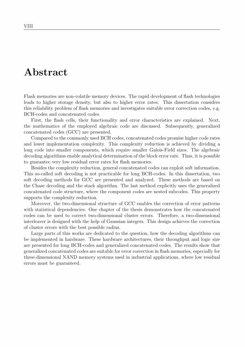
Abstract
Flash memories are non-volatile memory devices. The rapid development of flash technologiesleads to higher storage density, but also to higher error rates. This dissertation considersthis reliability problem of flash memories and investigates suitable error correction codes, e.g.BCH-codes and concatenated codes.
First, the flash cells, their functionality and error characteristics are explained. Next,the mathematics of the employed algebraic code are discussed. Subsequently, generalizedconcatenated codes (GCC) are presented.
Compared to the commonly used BCH codes, concatenated codes promise higher code ratesand lower implementation complexity. This complexity reduction is achieved by dividing along code into smaller components, which require smaller Galois-Field sizes. The algebraicdecoding algorithms enable analytical determination of the block error rate. Thus, it is possibleto guarantee very low residual error rates for flash memories.
Besides the complexity reduction, general concatenated codes can exploit soft information.This so-called soft decoding is not practicable for long BCH-codes. In this dissertation, twosoft decoding methods for GCC are presented and analyzed. These methods are based onthe Chase decoding and the stack algorithm. The last method explicitly uses the generalizedconcatenated code structure, where the component codes are nested subcodes. This propertysupports the complexity reduction.
Moreover, the two-dimensional structure of GCC enables the correction of error patternswith statistical dependencies. One chapter of the thesis demonstrates how the concatenatedcodes can be used to correct two-dimensional cluster errors. Therefore, a two-dimensionalinterleaver is designed with the help of Gaussian integers. This design achieves the correctionof cluster errors with the best possible radius.
Large parts of this works are dedicated to the question, how the decoding algorithms canbe implemented in hardware. These hardware architectures, their throughput and logic sizeare presented for long BCH-codes and generalized concatenated codes. The results show thatgeneralized concatenated codes are suitable for error correction in flash memories, especially forthree-dimensional NAND memory systems used in industrial applications, where low residualerrors must be guaranteed.

Zusammenfassung
Flashspeicher sind nichtfluchtige Speicherbausteine, deren rasante Entwicklung zu hoherenDichten und damit verbunden zu hoheren Fehlerraten fuhrt. Die Dissertation greift dieseProblematik auf und untersucht fur Flashspeicher geeignete Fehlerkorrekturverfahren, wieBCH-Codes und die verallgemeinerte Codeverkettung.
Zunachst wird auf die Flashzellen eingegangen, deren Funktionsweise und das resultierendeFehlerverhalten erlautert. Die Basis fur die Fehlerkorrektur bilden algebraische Codes, derenmathematische Grundlagen beschrieben werden. Im Anschluss wird die verallgemeinerteCodeverkettung vorgestellt.
Verkettete Codes ermoglichen eine hohere Coderate und geringere Implementierungskom-plexitat im Vergleich zu den bisher noch uberwiegend verwendeten BCH-Codes. Die Reduktionder Komplexitat folgt aus der Aufteilung langer Codeworte in kleinere Komponenten, die auf-grund der kleinen Galois Feldgroße mit geringem Aufwand decodiert werden konnen. Ihre alge-braische Dekodierung ermoglicht eine analytische Bestimmbarkeit der Blockfehlerrate. Daherkonnen die fur Flashspeicher erforderlichen geringen Restfehlerwahrscheinlichkeiten garantiertwerden.
Neben der geringeren Komplexitat ermoglicht die verallgemeinerte Codeverkettung aucheine Decodierung mit Zuverlassigkeitsinformation. Diese sogenannte Soft-Decodierung ist furlange BCH-Codes nicht mit vertretbarem Aufwand moglich. In dieser Dissertation werdenzwei Soft-Decodierverfahren vorgestellt und untersucht. Diese Verfahren basieren auf derChase-Decodierung und auf der Listendekodierung mittels Stack-Algorithmus. Letzteres Ver-fahren nutzt explizit die Struktur der verallgemeinerten Codeverkettung aus, bei der dieKomponenten-Codes aus einer Reihe von Teilcodes besteht. Diese Struktur hilft, die De-codierkomplexitat zu reduzieren.
Außerdem eignet sich die zweidimensionale Struktur der verallgemeinerten Codeverket-tung gut fur die Korrektur von Fehlermustern mit statischen Abhangigkeiten. Ein Kapitel derDissertation ist der Frage gewidmet, wie die Codeverkettung fur die Korrektur von zweidimen-sionalen Clusterfehlern verwendet werden kann. Dazu wird mithilfe von Gauß-Zahlen ein Inter-leaving bestimmt, das die Korrektur von Clusterfehlern mit maximalem Radius ermoglicht.
Desweitern widmet sich ein Großteil der Arbeit der Frage, wie diese Codierverfahrenmoglichst gunstig in Hardware implementiert werden konnen. Sowohl fur lange BCH-Codes alsauch fur die Decodierung der verketteten Codes werden Hardware-Architekturen entworfen,der erzielbare Durchsatz und der Flachenbedarf fur die Logikelemente bestimmt. Diese Ergeb-nisse belegen, dass die verallgemeinerte Codeverkettung fur die Fehlerkorrektur in Flashspe-ichern gut geeignet ist. Dies gilt insbesondere fur 3D-NAND Speichersysteme im industriellenEinsatz, die sehr niedrige Restfehlerwahrscheinlichkeiten gewahrleisten mussen.

XI
List of Acronyms
ARQ automatic repeat-requestASK amplitude shift keyingASIC application-specific integrated circuitAWGN additive white gaussian noiseBCH Bose Chaudhuri HocqenhemBER bit error rateBL bit lineBMA Berlekamp-Massey algorithmBMD bounded minimum distanceBWE bit write enableBSC binary symmetric channelBSEEC binary symmetric error and erasure channelCIRC Cross-interleaved Reed-Solomon CodeCD Compact DiscCF Compact FlashCPU central processing unitDFT discrete Fourier transformationDMA direct memory accessDP-SRAM dual-port static random-access memorySP-SRAM single-port static random-access memoryDVB-T terestrical digital video broadcastECC error correction codeEOL end of lifetimeFEC forward error correctionFER frame error rateFET field effect transistorFNT Fowler-Nordheim tunnelingFPGA field programmable gate arraysFG floating gateGCC generalized concatenated codeGE gate equivalentGF Galois fieldGSL ground selector lineHDD hard disc driveiBMA inversionless Berlekamp-Massey algorithmIDFT inverse discrete Fourier transformationJEDEC Joint Electron Device Engineering CouncilLDPC low-density parity checkLLR log-likelihood ratio
XII CONTENTS
LRP least reliable bit positionLP lower pageLFSR linear feedback shift registerLUT look-up tableML maximum-likelihoodMLC multi-level cellMMC Multimedia CardMP middle pageOFDM orthogonal frequency-division multiplexingPCIe Peripheral Component Interconnect ExpressQR quick response codeRAID redundant array of independent disksRBER raw bit error rateRS Reed-SolomonRSV Reed-Solomon/ViterbiSATA Serial AT AttachementSD Secure Digital Memory CardSLC single-level cellSNR signal to noise ratioSPC single parity checkSRAM static random-access memorySSD solid-state driveSSL sensing selector lineTLC triple-level cellUP upper pageUPIBA universal parallel inversionless Blahut algorithmUSB Universal Serial BusVLSI very large scale integrationWL word line
XIII
Nomenclature
A outer code
a, a(x) outer codeword vector/polynomial
B inner code
b, b(x) inner codeword vector/polynomial
C code
c, c(x) codeword vector/polynomial
d, da, db codeword distance
e, e(x) error vector/polynomial
g(x) generator polynomial
i, i(x) information vector/polynomial
k, ka, kb codeword dimension
L number of code levels
n, na, nb codeword size
p(x) primitive polynomial
r, r(x) received vector/polynomial
R code rate
r number of redundancy symbols
S, S(x) Syndrom values vector/polynomial
t, ta, tb error correction capability
? erasure symbol
α primitive element
ε channel error probability
λ channel erasure probability
Ω(x) error-value polynomial
σ(x) error-location polynomial

1
Chapter 1
Introduction
Thousands of years ago, stones were used to store information. Today, storage systems con-tinue their important role on the second most element on the earth crust, silicon (Si), theelement from which Flash memories are produced.
Medias are physical information carriers. The most common modern medias can be dividedinto optical or magnetic discs or tapes and Flash memories. In optical systems, mainly thesurface reflection or the transmittance of a photon source is measured. With the magnetic discsused in hard disk drives, the magnetic polarization of a surface is measured with coils. Flashmemory uses floating gates, where electrons can be loaded and unloaded into an insulatedgate using the tunnel effect. These non-volatile trapped electrons in the floating gate forman electrical field, which can be measured. The advantage of disc-based systems over Flashmemory is the absence of moving mechanical elements. At present, it can be observed that thedensity has increased over time while the reliability of storage systems typically has decreasedwith each new technology. As the silicon-based structure shrink is reaching its limits given bythe lattices, the so-called 3D technology tries to overcome this issue by increasing the layersof the die.
Each of these media share in common the fact that they are not absolutely accurate. Er-rors can occur during the writing and reading process as well as in idle state. An additionalchallenge in storage systems is that the sender cannot request retransmit erroneous data usingautomatic repeat-requests (ARQs), and thus forward error correction (FEC) codes are ap-plied. The error correction ensures that the requirements regarding the reliability for a givenapplication are met. In coding theory, many error correction codes (ECCs) exists with dif-ferent properties that can be divided into complexity characteristics and their error correctionperformance. As already mentioned, the provable error correction boundaries are an impor-tant property. In order to check whether a code is applicable it can be simulated or analyzedanalytically. Simulation is possible if the target error rate is high. If a code has to be testedfor a very low error rate, the simulation can exceed all available resources such as time andcosts. Algebraic codes are then taken into account. These codes can be decoded with boundedminimum distance (BMD) decoding, where the residual error rate can be calculated. BoseChaudhuri Hocqenhem (BCH) and Reed-Solomon (RS) codes are the most famous algebraiccodes.
NAND flash memories are important components in embedded systems as well as consumerelectronics. The flash cells keep their electrical charge without a power supply. However,errors may occur while the information is read. Consequently, error correction coding ECCis required to ensure data integrity and reliability for the user data [51, 63, 16]. In the past,mostly BCH codes with hard-input algebraic decoding were used for error correction [51, 76]and [83].
2 CHAPTER 1. INTRODUCTION
Reliability information about the state of the cell can significantly improve the ECC perfor-mance [17]. Soft-input decoding algorithms are required to exploit the reliability information.For instance, low-density parity check (LDPC) can provide strong error-correcting performancein NAND flash memories [77, 68, 43, 32, 30, 79]. However, the implementation complexity ofan LDPC decoder can be high when high data throughput should be achieved. Concatenatedcodes constructed from long BCH codes can achieve low residual error rates [13, 36, 37], al-though they require very long codes and hence a long decoding latency, which might not beacceptable for all applications of flash memories. LDPC codes have high residual error rates(the error floor) and are not suitable for applications that require very low decoder failure prob-abilities [81]. For instance, the Joint Electron Device Engineering Council (JEDEC) standardfor solid-state drive (SSD) recommends an uncorrectable bit error rate of less than 10−15 forclient applications and of less than 10−16 for enterprise solutions [1]. For some applications,block error rates less than 10−16 are required [41].
1.1 Goals
The initial impulse of this work was the demand of improvements of error correction codesfor Flash memories in industrial applications. This impulse triggered a first investigation ofseveral code types and their performances, which led to the design of an ECC candidate andfinally its implementation in hardware [81]. The choice of an ECC candidate is determinedby the industrial requirements, placing an emphasis on the verifiability of the error correctioncapability. Additional requirements for mass-storage systems include the ECCs demand foroverhead, costs for implementation and throughput.
From this preliminary investigation, the generalized concatenated code (GCC) emerged asa favorite. In this work, the code construction and its underlying theory will be explained andit will be described why this code is suitable for industrial applications. Subsequently, a strongfocus of this work lies on the implementation of the necessary algorithms in field programmablegate arrayss (FPGAs) and application-specific integrated circuit (ASIC), where the aspects ofarea and throughput are highlighted.
We demonstrate that GCC can achieve such low residual error rates. ECC based on GCChas a high potential for various applications in data communication and data storage systems,e.g. for digital magnetic storage systems [20] and non-volatile flash memories [81, 92]. Thesecodes are typically constructed from short inner binary BCH codes and outer RS codes [19,80]. Hence, the hard-input decoding is based on low-complexity algebraic decoding. Newconstructions have recently proposed that enable higher code rates [98] and [78], where theinner codes are extended BCH codes. In particular, single parity check (SPC) codes are usedin the first level of the GCC. A soft-input decoding algorithm for GCC was proposed in [97],where the decoding is based on sequential stack decoding of the inner codes.
1.2 Thesis Structure
This thesis starts with the brief presentation of several modern storage medias, their func-tionality and error characteristics in Chapter 2. It then concentrates on Flash memories anddescribes error models that are used to design ECC codes.
Chapter 3 offers an introduction to algebraic codes and its basis are introduced, namelythe Galois fields. This is the preliminary for the GCC encoding decoding scheme as its errorbounds and code parameter design, which is described in Chapter 4.
1.2. THESIS STRUCTURE 3
In Chapter 5, an interleaving concept based on Gaussian integers combined with GCCcodes is presented that can decode special shaped burst errors. This work was published in[86, 84, 85].
The algebraic decoder described in chapters 3 and 4 is limited to decoding informationwith binary quantization, also called hard information. In Chapter 6, techniques and their usefor GCC are introduced, which enable higher quantization levels and thus increases the errorcorrection performance. Research in constructing high-rate was published in [97].
Chapters 7, 8 and 9 describe the hardware implementation of the algorithms. In [82, 95, 83],an efficient algebraic decoder for large block size BCH codes are published. Its architecture,impact on complexity and throughput is discussed in Chapter 7. The implementation andits analysis for hard information GCC en- and decoder in very large scale integration (VLSI)is described in Chapter 8. Publications on hard information GCC implementations include[91, 99, 92]. This GCC implementation is then extended by a soft information decoder inChapter 9, which were published in [96, 87, 93, 94, 98, 101].
4
Chapter 2
Media and Channel Models
Storage medias are carriers that store information in a non-volatile manner over a periodof time. This chapter provides an overview of modern storage medias, its functionality andchannel models. In Section 2.2, the focus lies on Flash memories. Using these devices willlead to the problem that the original information is disturbed by several effects that evengrow over the lifetime of this memory. In order to encounter the problem of erroneous datathat is read back from a device, ECCs are used. A huge variety of ECC types exist withdifferent parameters. A proper choice is essential to address the demands for different areassuch as industrial applications where a provable error bound is an important requirement. InSection 2.2.4, channel models are discussed to assess this either analytically or these curvesare measured by Monte Carlo simulation. At the end of this chapter, the reader will know whyerrors in Flash memories occur and how they can be modeled. Because there are similaritieswith other carriers magnetic and optical carriers are also considered in Section 2.3.
2.1 Storage systems
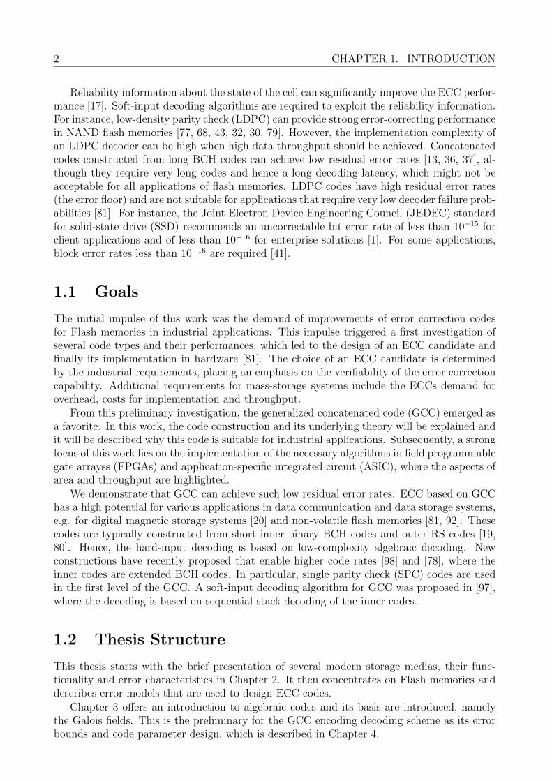
In systems like mobile phones, cloud storage, different-scaled computers, embedded systemsand others, non-volatile memories are integrated. An example combination for Flash storagesystems is depicted in Figure 2.1, which shows three components: Flash device, Flash microcontroller and a host. The Flash device is connected via the Flash channel with a micro con-troller’s Flash interface that is connected using the host channel with a host. A standardizedFlash interface is specified in [56]. Further examples for links between the host and microcontroller are SATA, USB, PCIe or SD, where each standard has different application areas.For data transportation, storage systems with pluggable links like USB-sticks or SD-cards areavailable. In some cases, the carrier is a removable device that must be read by a readingdevice, like floppy discs, CDs, MMCs or quick response code (QR) codes on different materi-als. Therefore, the reading device comprises a micro controller that provides the interfacingbetween the carrier and other systems. A common Flash micro controller has a CPU runningfirmware on it that manages the data stored on the devices and controls the communication inboth directions between the host and device. Further modules serve features like cryptography,DMA mechanisms, data compression and error correction.
Application areas of memories are manifold. Some examples of data that is stored includemeasurements, personal data, accounting information, operating systems and programs. Afew application examples are the control logic for robot arms, medical instruments, routers,cellphone base stations, large machine control units, drill heads and automotive navigationsystems.
2.2. FLASH MEMORIES 5
host
inte
rfac
e
flash deviceCPU, ECC, crypto ...
microcontroller
flash
inte
rfac
e
host host channel Flash channel
Fig. 2.1: Flash microcontroller
Similar to the applications, its requirements are also manifold. High storage capacity anddata density or high reliability and data throughput are some examples. An additional factoris the data overhead needed for the data management and the redundancy for error correction.Moreover, data integrity, data encryption and long time storage are subjects that have to betaken into account. Similar to an ECC, the entire storage system has to be designed dependingon its requirements given by the application.
In order to provide an introduction to storage devices with different carrier materials, thefollowing sub-sections present four categories of storage devices.
2.2 Flash Memories
Flash memories are silicon-based semiconductors that can store data in a non-volatile manner.The first models were presented by Fuji Masuoka (Thoshiba) in 1984. They are dividedinto NAND and NOR technology, where NAND memories are used for mass storage andNOR traditionally for code storage due to the faster access time. Nowadays developmentis proceeding towards higher density by shrinking the silicon structure size and using morelayers, called the 3D-NAND Flash memory.
2.2.1 Flash Cell
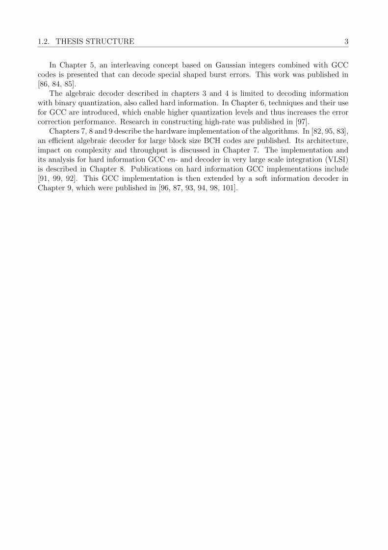
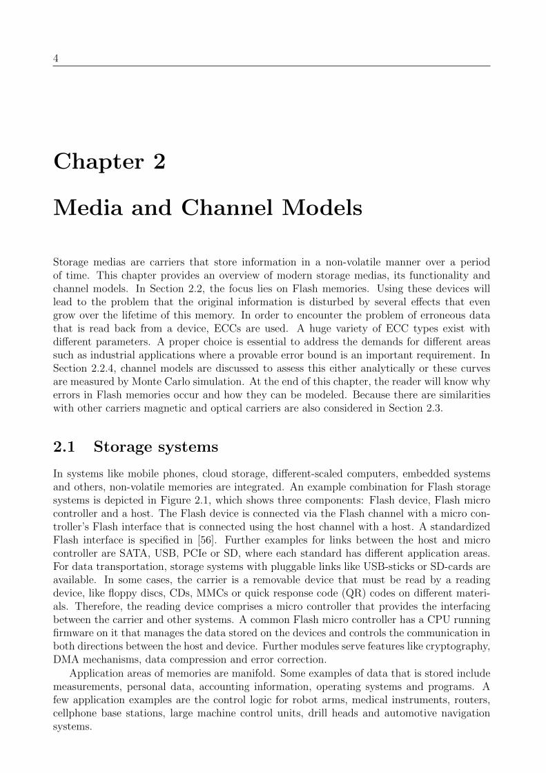
Figure 2.2 shows a floating gate (FG) cell. It is similar to a FET and comprises four connectingelements, source, drain, control gate and the bulk substrate. An additional FG is surroundedby isolating oxide between the control gate and the substrate. This isolation makes thisFG an electron trap that holds information for a longer time period [51]. An FG has threebasic functionalities, namely reading, writing and erasing the FG state. Figure 2.3 depictsFGs in a NAND matrix. In one dimension, these cells are connected in series. One of theseseries comprising several NANDs is called a bit line (BL). In the other dimension, all gatesare connected in parallel to a word line (WL), which represents a page. All pages that areconnected with the same BL are called a Flash block. The ground selector line (GSL) and thesensing selector line (SSL) are necessary to apply the different read, write and erase modes.A Flash memory die comprises several Flash blocks.
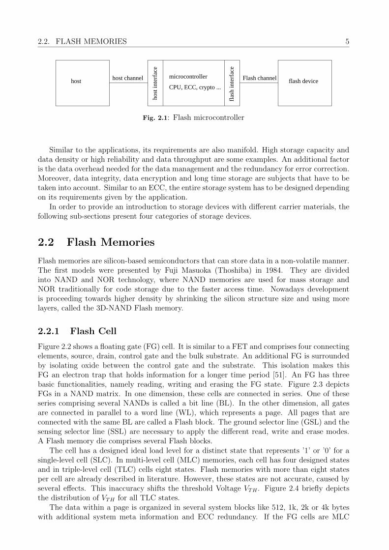
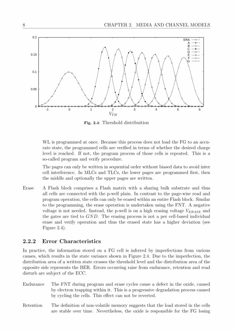
The cell has a designed ideal load level for a distinct state that represents ’1’ or ’0’ for asingle-level cell (SLC). In multi-level cell (MLC) memories, each cell has four designed statesand in triple-level cell (TLC) cells eight states. Flash memories with more than eight statesper cell are already described in literature. However, these states are not accurate, caused byseveral effects. This inaccuracy shifts the threshold Voltage VTH . Figure 2.4 briefly depictsthe distribution of VTH for all TLC states.
The data within a page is organized in several system blocks like 512, 1k, 2k or 4k byteswith additional system meta information and ECC redundancy. If the FG cells are MLC

6 CHAPTER 2. MEDIA AND CHANNEL MODELS
Oxide
Oxide
Floating Gate
Control Gate
SourceDrain
P SubstrateN WellP Well
Fig. 2.2: Floating Gate
GSL
SSL
BL0
BL1
BL2
BLM
WL0
WL1
WL2
WLN
Fig. 2.3: NAND structure

2.2. FLASH MEMORIES 7
ERA A B C D E F G
LP 1 1 1 1 0 0 0 0
MP 1 1 0 0 0 0 1 1
UP 1 0 0 1 1 0 0 1
(a)
ERA A B C D E F G
LP 1 0 0 0 0 1 1 1
MP 1 1 0 0 1 1 0 0
UP 1 1 1 0 0 0 0 1
(b)
Tab. 2.1: Flash state level encoding with (a) 1:2:4 and (b) 2:3:2 levels
or TLC, an WL represents a shared page that comprises two or three pages with the sameelectrical address but different logical addresses with a special arrangement such that a writingcauses a low electrical bias [7]. These pages are named lower page (LP), middle page (MP)and upper page (UP). A system block does not cross into different page levels.
The FG states of a TLC are the erased state ERA and the programmed statesA,B,C,D,E, F,G. Two exemplar different state-level encodings are shown in Table 2.1.Depending on the page level the reference voltage is between different state levels. In Ta-ble 2.1(a), the LP reference is between C and D, and MP between A and B, E and F . Underthe assumption of random data, the encoding (a) has a smaller bit error rate (BER) in theLP, a moderate BER in the MP and its highest BER in the UP. An alternative encoding isshown in (b) where, in comparison to (a), the LP and MP has an increased BER but the UPlevel has a lower BER.
In order to understand the electrical circuit of a NAND Flash memory, we briefly presentthe basic access functions for the FGs:
Read In the read operation, the cell gates in an WL that is read is put to VREAD while allother WL are tied to VPASS,R. Only the electrical load from the FG cell that is inread mode affects the current that flows through the BL. This current is measuredusing an integrator circuit and a configurable threshold voltage VTH .
VTH has to be determined by either a built-in mechanism inside the Flash memoryor with single state reads from the Flash controller. With these single state reads,the controller scans the changes of ones to zeros with fine-grained VTH steps. Forsymmetric error probabilities, the optimal VTH for a distinct state level is where thechange from one to zero between two VTH steps is minimal.
If information is read with additional reliability information, several offsets per statelevel are read. This results in soft bits for each information (hard) bit. Because thedistributions of the state levels vary, it also holds interest which state level was read.This information is converged by the level indicator bits. Figure 2.4 shows the VTHdistribution and Figure 2.6 exemplar soft information thresholds for one level.
Program The programming operation tunnels electrons onto the FG using the Fowler-Nordheim tunneling (FNT). An electron injection is triggered with the followingconfiguration. All unselected gates in the BLs are in passing mode with VPASS,P ,the selected gates within a WL are connected to a much higher gate voltage VPRG.Those BLs that are programmed are tied to GND and all others are on VDD. An
8 CHAPTER 2. MEDIA AND CHANNEL MODELS
0
0.05
0.1
0.15
0.2
-1 0 1 2 3 4 5 6
ERAABCDEFG
VTH
Fig. 2.4: Threshold distribuition
WL is programmed at once. Because this process does not load the FG to an accu-rate state, the programmed cells are verified in terms of whether the desired chargelevel is reached. If not, the program process of those cells is repeated. This is aso-called program and verify procedure.
The pages can only be written in sequential order without biased data to avoid intercell interference. In MLCs and TLCs, the lower pages are programmed first, thenthe middle and optionally the upper pages are written.
Erase A Flash block comprises a Flash matrix with a sharing bulk substrate and thusall cells are connected with the p-well plain. In contrast to the page-wise read andprogram operation, the cells can only be erased within an entire Flash block. Similarto the programming, the erase operation is undertaken using the FNT. A negativevoltage is not needed. Instead, the p-well is on a high erasing voltage VERASE andthe gates are tied to GND. The erasing process is not a per cell-based individualerase and verify operation and thus the erased state has a higher deviation (seeFigure 2.4).
2.2.2 Error Characteristics
In practice, the information stored on a FG cell is inferred by imperfections from variouscauses, which results in the state variance shown in Figure 2.4. Due to the imperfection, thedistribution area of a written state crosses the threshold level and the distribution area of theopposite side represents the BER. Errors occurring raise from endurance, retention and readdisturb are subject of the ECC.
Endurance The FNT during program and erase cycles cause a defect in the oxide, causedby electron trapping within it. This is a progressive degradation process causedby cycling the cells. This effect can not be reverted.
Retention The definition of non-volatile memory suggests that the load stored in the cellsare stable over time. Nevertheless, the oxide is responsible for the FG losing
2.2. FLASH MEMORIES 9
electrons. Practically information stored on other medias suffer the same prob-lem of transience. The time period that can be supported strongly depends onthe device temperature. At a normal room temperature of 300K, the errorcorrection capability limit is reached within years. A so-called baked device at360K reaches this limit within a few days. For testing the degradation in Flashmemory devices, special baking procedures are used. In order to reload the FG,a rewrite after a specified time period, which is set in the firmware, is used torefresh the information.
Read disturb The read voltage disturbs neighboring cells due to its electrical field. Unfortu-nately, the writing process has a higher impact because it has a higher operationvoltage, although it occurs less often than cell reads. This read disturb is han-dled by rewriting cells after a specific number of reads.
Media defect Different causes lead to total defect of an entire die, e.g. the defect of the chargepipes that are needed for VPRG and VERASE. This problem is encountered byredundant data storage in different dies or chips using a redundant array ofindependent disks (RAID).
Radiation Several radiations cause mutations of the cell load and thus a threshold shift [28].This holds interest in several environments like space, where cosmic ray is muchmore intensive. Possible correlated errors are thinkable caused by radiationtrails. Their influence in GCC is not investigated in this work and might beinteresting for further research.
In various publications [38, 60, 8], the investigations of the Flash channel error and itscharacteristics shows in common a per-bit statistical independence and that an additive whitegaussian noise (AWGN) channel model can be assumed.
2.2.3 Flash Layer Design
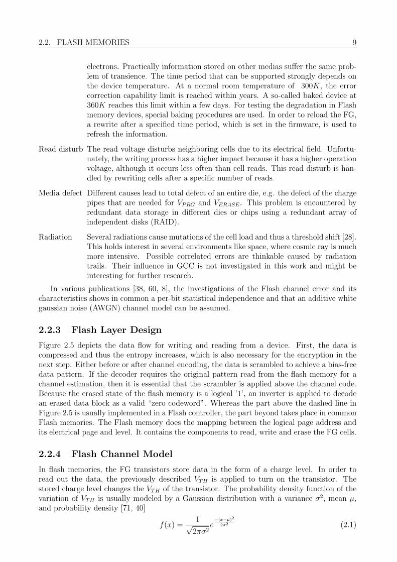
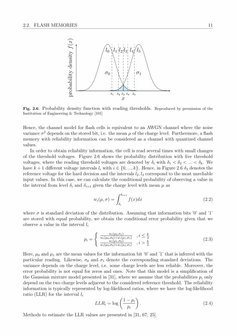
Figure 2.5 depicts the data flow for writing and reading from a device. First, the data iscompressed and thus the entropy increases, which is also necessary for the encryption in thenext step. Either before or after channel encoding, the data is scrambled to achieve a bias-freedata pattern. If the decoder requires the original pattern read from the flash memory for achannel estimation, then it is essential that the scrambler is applied above the channel code.Because the erased state of the flash memory is a logical ’1’, an inverter is applied to decodean erased data block as a valid “zero codeword”. Whereas the part above the dashed line inFigure 2.5 is usually implemented in a Flash controller, the part beyond takes place in commonFlash memories. The Flash memory does the mapping between the logical page address andits electrical page and level. It contains the components to read, write and erase the FG cells.
2.2.4 Flash Channel Model
In flash memories, the FG transistors store data in the form of a charge level. In order toread out the data, the previously described VTH is applied to turn on the transistor. Thestored charge level changes the VTH of the transistor. The probability density function of thevariation of VTH is usually modeled by a Gaussian distribution with a variance σ2, mean µ,and probability density [71, 40]
f(x) =1√
2πσ2e−(x−µ)2
2σ2 (2.1)
10 CHAPTER 2. MEDIA AND CHANNEL MODELS
source encoder
encryption
scrambling
channel encoder
source decoder
decryption
descrambling
channel decoder
D/A conversion A/D conversion
mapping to mapping from
shared page shared page
flash cellsN
Fig. 2.5: Channel abstraction layers
2.2. FLASH MEMORIES 11
δ4 δ5δ2δ1 δ3
σ0 σ1
l0 l1 l2 l3 l4 l5
x
pro
bab
ilit
yd
ensi
tyf
(x)
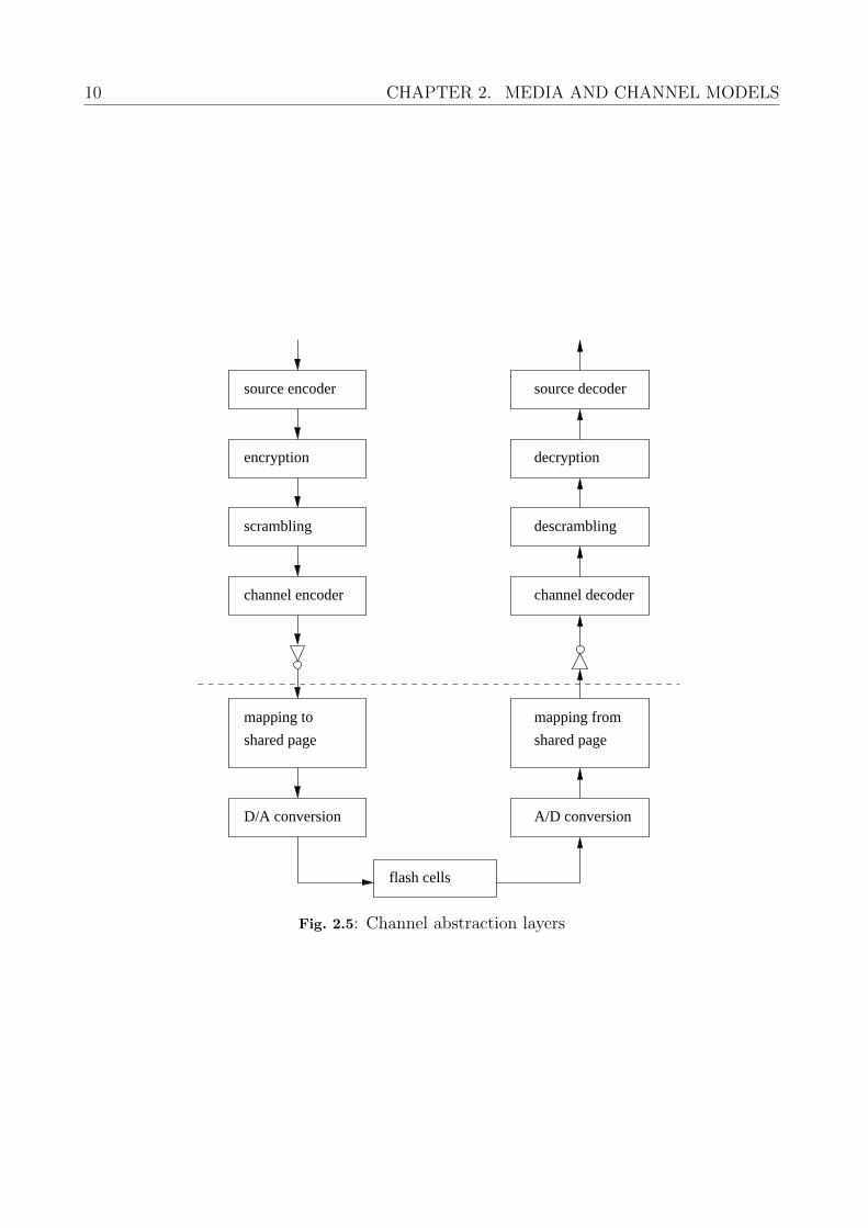
Fig. 2.6: Probability density function with reading thresholds. Reproduced by permission of theInstitution of Engineering & Technology [101]
Hence, the channel model for flash cells is equivalent to an AWGN channel where the noisevariance σ2 depends on the stored bit, i.e. the mean µ of the charge level. Furthermore, a flashmemory with reliability information can be considered as a channel with quantized channelvalues.
In order to obtain reliability information, the cell is read several times with small changesof the threshold voltages. Figure 2.6 shows the probability distribution with five thresholdvoltages, where the reading threshold voltages are denoted by δi with δ1 < δ2 < ... < δk. Wehave k+ 1 different voltage intervals li with i ∈ 0, ..., k. Hence, in Figure 2.6 δ3 denotes thereference voltage for the hard decision and the intervals l2, l3 correspond to the most unreliableinput values. In this case, we can calculate the conditional probability of observing a value inthe interval from level δi and δi+1 given the charge level with mean µ as
wi(µ, σ) =
∫ δi+1
δi
f(x)dx (2.2)
where σ is standard deviation of the distribution. Assuming that information bits ’0’ and ’1’are stored with equal probability, we obtain the conditional error probability given that weobserve a value in the interval li
pi =
wi(µ0,σ1)
wi(µ0,σ0)+wi(µ1,σ1), i ≤ k
2wi(µ1,σ0)
wi(µ0,σ0)+wi(µ1,σ1), i > k
2
(2.3)
Here, µ0 and µ1 are the mean values for the information bit ’0’ and ’1’ that is inferred with theparticular reading. Likewise, σ0 and σ1 denote the corresponding standard deviations. Thevariance depends on the charge level, i.e. some charge levels are less reliable. Moreover, theerror probability is not equal for zeros and ones. Note that this model is a simplification ofthe Gaussian mixture model presented in [31], where we assume that the probabilities pi onlydepend on the two charge levels adjacent to the considered reference threshold. The reliabilityinformation is typically represented by log-likelihood ratios, where we have the log-likelihoodratio (LLR) for the interval li
LLRi = log
(1− pipi
). (2.4)
Methods to estimate the LLR values are presented in [31, 67, 25].
12 CHAPTER 2. MEDIA AND CHANNEL MODELS
2.3 Other Modern Storage Systems
In order to provide an introduction to storage devices with different carrier materials, thefollowing subsections present an outtake of four storage devices.
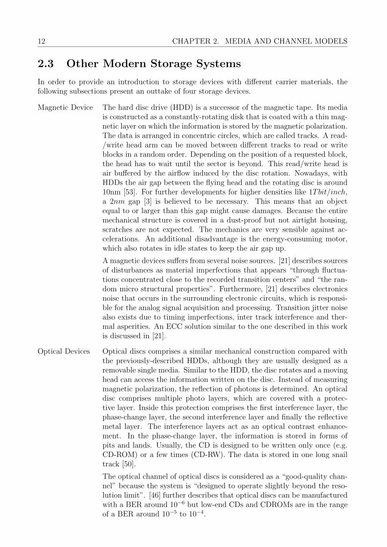
Magnetic Device The hard disc drive (HDD) is a successor of the magnetic tape. Its mediais constructed as a constantly-rotating disk that is coated with a thin mag-netic layer on which the information is stored by the magnetic polarization.The data is arranged in concentric circles, which are called tracks. A read-/write head arm can be moved between different tracks to read or writeblocks in a random order. Depending on the position of a requested block,the head has to wait until the sector is beyond. This read/write head isair buffered by the airflow induced by the disc rotation. Nowadays, withHDDs the air gap between the flying head and the rotating disc is around10nm [53]. For further developments for higher densities like 1Tbit/inch,a 2nm gap [3] is believed to be necessary. This means that an objectequal to or larger than this gap might cause damages. Because the entiremechanical structure is covered in a dust-proof but not airtight housing,scratches are not expected. The mechanics are very sensible against ac-celerations. An additional disadvantage is the energy-consuming motor,which also rotates in idle states to keep the air gap up.
A magnetic devices suffers from several noise sources. [21] describes sourcesof disturbances as material imperfections that appears “through fluctua-tions concentrated close to the recorded transition centers” and “the ran-dom micro structural properties”. Furthermore, [21] describes electronicsnoise that occurs in the surrounding electronic circuits, which is responsi-ble for the analog signal acquisition and processing. Transition jitter noisealso exists due to timing imperfections, inter track interference and ther-mal asperities. An ECC solution similar to the one described in this workis discussed in [21].
Optical Devices Optical discs comprises a similar mechanical construction compared withthe previously-described HDDs, although they are usually designed as aremovable single media. Similar to the HDD, the disc rotates and a movinghead can access the information written on the disc. Instead of measuringmagnetic polarization, the reflection of photons is determined. An opticaldisc comprises multiple photo layers, which are covered with a protec-tive layer. Inside this protection comprises the first interference layer, thephase-change layer, the second interference layer and finally the reflectivemetal layer. The interference layers act as an optical contrast enhance-ment. In the phase-change layer, the information is stored in forms ofpits and lands. Usually, the CD is designed to be written only once (e.g.CD-ROM) or a few times (CD-RW). The data is stored in one long snailtrack [50].
The optical channel of optical discs is considered as a “good-quality chan-nel” because the system is “designed to operate slightly beyond the reso-lution limit”. [46] further describes that optical discs can be manufacturedwith a BER around 10−6 but low-end CDs and CDROMs are in the rangeof a BER around 10−5 to 10−4.
2.4. SUMMARY 13
In contrast to HDDs, the CDs underlie different physical stress likescratches and dust. Most of these irritations draw an erroneous line overthe stored data, which leads to an error burst characteristic. A radial-oriented scratch tends to generate single errors over several blocks, whereasconcentric scratches tend to create burst errors. Depending on the orien-tation of the same scratch shape, there are drastic differences for the errorcorrection demands. A classical approach to encounter this problem isinterleaving.
CD audio was introduced in the early-1980’ by Philips and Sony. It deploysthe Cross-interleaved Reed-Solomon Code (CIRC). This specific RS codecomprises 255 symbols with a size of eight bits and can correct up to foursymbol errors or eight as defect declared symbols. In order to avoid largerburst errors, interleaving is used.
Solid State Device SSD are successors of the HDDs. The name solid stands for storing dataon semiconductor materials instead of drives with moving parts, tubes,relays, etc. This makes it robust against mechanical stress. Because SSDsare developed as successors of HDDs their form factor and interface aresimilar but not necessary the same. Their random access time is less thanthe HDD because a readjustment of the reading head is not necessary.Overall they have a higher throughput. As SATA interfaces were common,faster PCIe are upcoming to the end of the 2010s, which is the result ofthe performance increase.
In contrast to other Flash memory storage systems like CF cards, SD cardsand USB sticks the SSD is designed for large storage capacity. An SSDsystem comprises a Flash controller with a multi-core processor, servingseveral Flash dies in multiple Flash channels. Common systems comprisesfour or eight channels, each with eight, sixteen or more dies. In enterprisesystems, the flash controller manages 128, 256 or 512 Flash dies [52].
Matrix Barcode Matrix barcodes are two-dimensional codes. A famous example of such acode is the QR code, which has different levels of error correction capability.They are applied to various objects made of different materials like paper,metal, synthetics, etc. Some considerations on how to apply GCC with anoptimal interleaving mechanism on this code class are discussed in Chapter5.
2.4 Summary
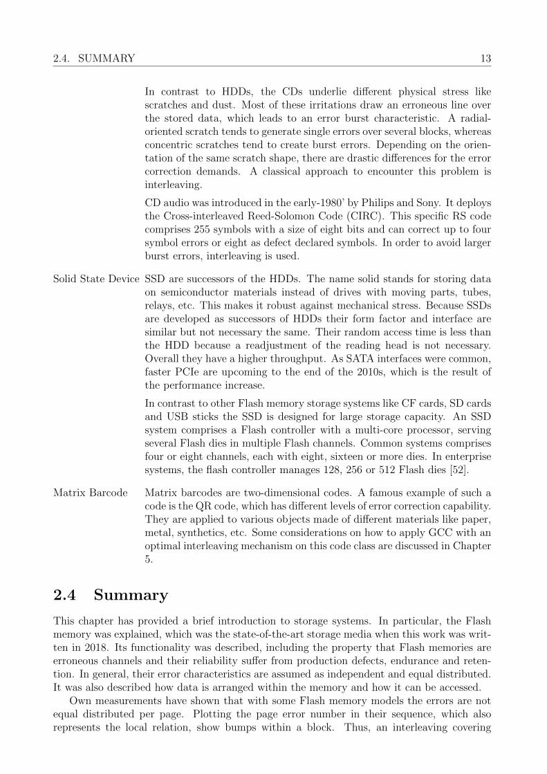
This chapter has provided a brief introduction to storage systems. In particular, the Flashmemory was explained, which was the state-of-the-art storage media when this work was writ-ten in 2018. Its functionality was described, including the property that Flash memories areerroneous channels and their reliability suffer from production defects, endurance and reten-tion. In general, their error characteristics are assumed as independent and equal distributed.It was also described how data is arranged within the memory and how it can be accessed.
Own measurements have shown that with some Flash memory models the errors are notequal distributed per page. Plotting the page error number in their sequence, which alsorepresents the local relation, show bumps within a block. Thus, an interleaving covering

14 CHAPTER 2. MEDIA AND CHANNEL MODELS
several pages would increase the decoding performance. Because the data is then distributedover different pages the performance will suffer.
From a coding theorist perspective, it would be highly efficient to apply multi-level codingto achieve higher error correction performance. Multi-level codes can be applied using thethreshold voltage as an amplitude shift keying (ASK). At present, there are no Flash memorieson the market that support such a multilevel coding. The structure of the existing sharedpages is historically grown. This topic should be targeted in future research.
Finally other storage media, their components and challenges in data reliability were dis-cussed. Similar to the Flash memory, they suffer from an erroneous channel and ECCs areapplied. For this and further work they hold interest due to their two-dimensional informa-tion arrangement. In the case of correlated errors techniques from Chapter 5 could be usedto increase the error correction capability.
15
Chapter 3
Preliminaries for Channel Coding
A channel model that represents the Flash memory can be modeled by a source emittinginformation, the transmission channel that adds noise and a receiving sink. In Chapter 2 theFlash memory and its error sources were discussed. In order to encounter the data corruptionat the sink, channel codes that correct errors by adding redundancy are applied. Severalchannel code classes exist, which in turn also have a high range of decoding algorithms withdifferent properties. The effect of channel codes is that the number of errors of a receivedmessage is reduced. This chapter provides a basic introduction to algebraic codes that canbe decoded with BMD and thus an analytical determination of the residual error rate can bemade. The aim of this chapter is to offer an introduction to algebraic codes. An importantbase is the Galois field (GF), which enables basic operations on finite symbols. Section 3.1provides an overview of GF with some examples and implementation approaches. Section 3.2explains the algebraic code. Based on this, a basic error model is presented in Section 3.3.
3.1 Galois Fields
GF provide the mathematical operations that are necessary for algebraic codes over a finiteset of symbols.
Definition 1. Group [6]A group A is a set of elements combined with an operand ∗, iff:
I Closure ∀a,b∈A : a ∗ b ∈ AII Associativity ∀a,b,c∈A : a ∗ (b ∗ c) = (a ∗ b) ∗ c
III Identity element ∃e∈A : ∀a∈A : a ∗ e = a
IV inverse element ∀a∈A : ∃b∈A : a ∗ b = e
If commutativity (∀a,b∈A : a ∗ b = b ∗ a) holds, it is called an Abeilan group.
Definition 2. Ring [6]A set A combined with two operands + and · is a ring, iff:
I A is an Abelian group regarding +
II Closure with respect to · in A : ∀a,b∈A : a · b ∈ AIII Associativity of · : ∀a,b,c∈A : a · (b · c) = (a · b) · cIV Distributivity : ∀a,b,c∈A : a · (b+ c) = a · b+ a · c
16 CHAPTER 3. PRELIMINARIES FOR CHANNEL CODING
Definition 3. Field [6]A is a field, iff:
I Abelian group with respect to addition
II A without the zero element is an Abelian group with respect to multiplication
III Distributivity : ∀a,b,c∈A : a · (b+ c) = a · b+ a · c
Definition 4. Prime field [6]The GF is a field with finite number of elements. Let p ∈ N be prime. The set of elements0, 1, . . . , p− 1 with the operations (+, ·) mod p satisfies the axioms of a field and is called aprime field and denoted with GF (p).
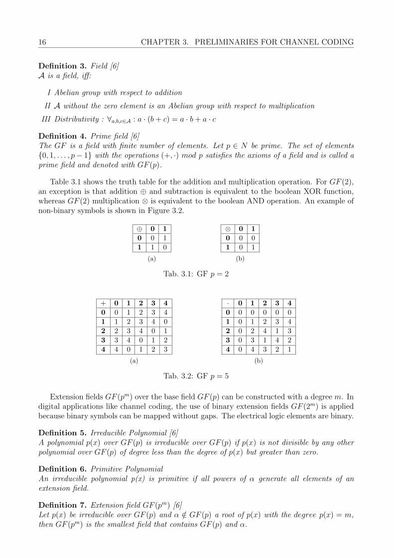
Table 3.1 shows the truth table for the addition and multiplication operation. For GF (2),an exception is that addition ⊕ and subtraction is equivalent to the boolean XOR function,whereas GF (2) multiplication ⊗ is equivalent to the boolean AND operation. An example ofnon-binary symbols is shown in Figure 3.2.
⊕ 0 1
0 0 1
1 1 0
(a)
⊗ 0 1
0 0 0
1 0 1
(b)
Tab. 3.1: GF p = 2
+ 0 1 2 3 4
0 0 1 2 3 4
1 1 2 3 4 0
2 2 3 4 0 1
3 3 4 0 1 2
4 4 0 1 2 3
(a)
· 0 1 2 3 4
0 0 0 0 0 0
1 0 1 2 3 4
2 0 2 4 1 3
3 0 3 1 4 2
4 0 4 3 2 1
(b)
Tab. 3.2: GF p = 5
Extension fields GF (pm) over the base field GF (p) can be constructed with a degree m. Indigital applications like channel coding, the use of binary extension fields GF (2m) is appliedbecause binary symbols can be mapped without gaps. The electrical logic elements are binary.
Definition 5. Irreducible Polynomial [6]A polynomial p(x) over GF (p) is irreducible over GF (p) if p(x) is not divisible by any otherpolynomial over GF (p) of degree less than the degree of p(x) but greater than zero.
Definition 6. Primitive PolynomialAn irreducible polynomial p(x) is primitive if all powers of α generate all elements of anextension field.
Definition 7. Extension field GF (pm) [6]Let p(x) be irreducible over GF (p) and α /∈ GF (p) a root of p(x) with the degree p(x) = m,then GF (pm) is the smallest field that contains GF (p) and α.
3.1. GALOIS FIELDS 17
In the context of coding theory, sometimes a polynomial is expressed as a vector. Therefore,the bijective relation is used as
a = (a0, a1, . . . , an−1)←→ a(x) = a0 + a1x+ . . .+ an−1xn−1. (3.1)
Definition 8. discrete Fourier transformation (DFT)The DFT for a polynomial A(x) with coefficients α from GF is:
ai = A(αi), i = 0, . . . , n− 1 (3.2)
and its inverse discrete Fourier transformation (IDFT) is:
Aj = n−1 · a(α−j), j = 0, . . . , n− 1 (3.3)
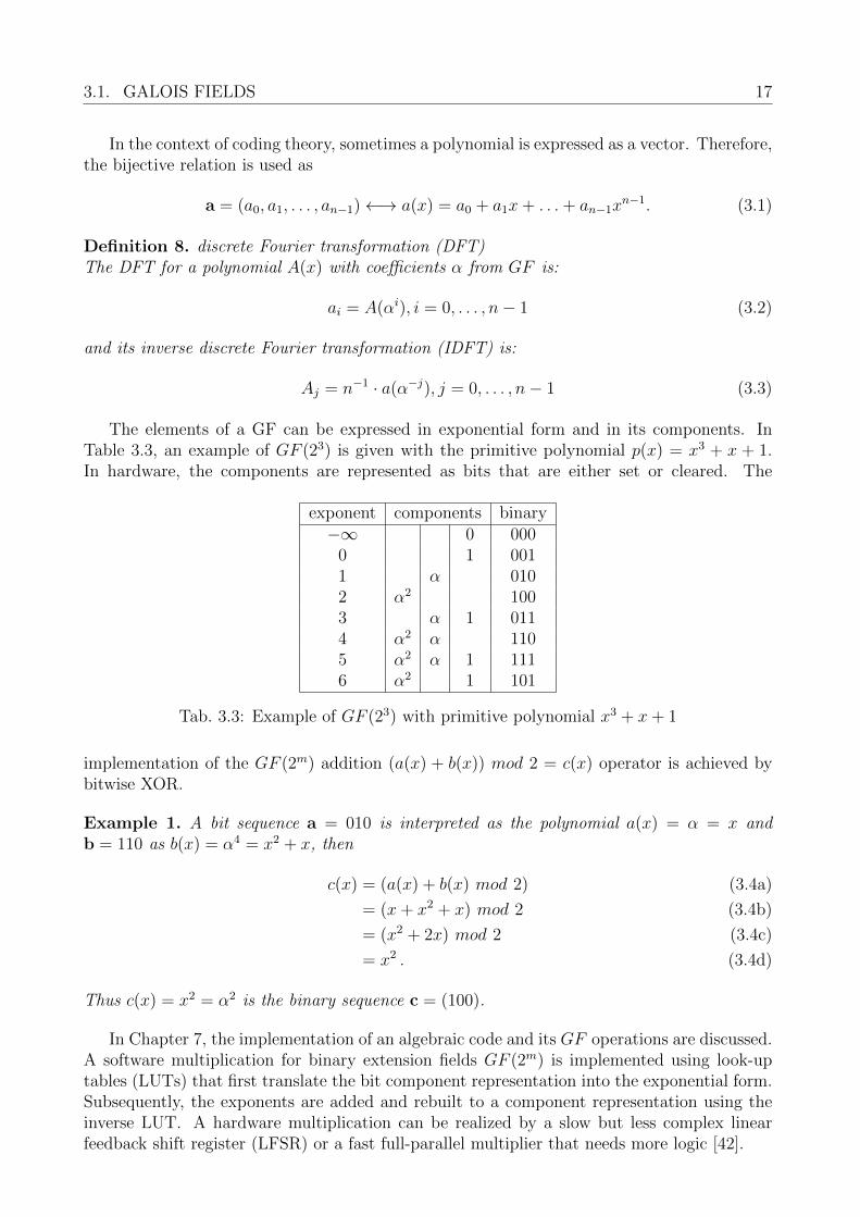
The elements of a GF can be expressed in exponential form and in its components. InTable 3.3, an example of GF (23) is given with the primitive polynomial p(x) = x3 + x + 1.In hardware, the components are represented as bits that are either set or cleared. The
exponent components binary−∞ 0 000
0 1 0011 α 0102 α2 1003 α 1 0114 α2 α 1105 α2 α 1 1116 α2 1 101
Tab. 3.3: Example of GF (23) with primitive polynomial x3 + x+ 1
implementation of the GF (2m) addition (a(x) + b(x)) mod 2 = c(x) operator is achieved bybitwise XOR.
Example 1. A bit sequence a = 010 is interpreted as the polynomial a(x) = α = x andb = 110 as b(x) = α4 = x2 + x, then
c(x) = (a(x) + b(x) mod 2) (3.4a)
= (x+ x2 + x) mod 2 (3.4b)
= (x2 + 2x) mod 2 (3.4c)
= x2 . (3.4d)
Thus c(x) = x2 = α2 is the binary sequence c = (100).
In Chapter 7, the implementation of an algebraic code and its GF operations are discussed.A software multiplication for binary extension fields GF (2m) is implemented using look-uptables (LUTs) that first translate the bit component representation into the exponential form.Subsequently, the exponents are added and rebuilt to a component representation using theinverse LUT. A hardware multiplication can be realized by a slow but less complex linearfeedback shift register (LFSR) or a fast full-parallel multiplier that needs more logic [42].
18 CHAPTER 3. PRELIMINARIES FOR CHANNEL CODING
3.2 Channel Coding Basics
Channel codes expand information with additional redundancy and are used to protect theinformation against errors such that they can be decoded by FEC. There are two main differentapproaches. The first domain is formed by the convolutional codes where the message bitsdepend on µ previous data bits. They have their strength in correcting correlated errors. Theother code domain is block codes, which convert information of k-bits into a block codewordof n bits. It has its strength in decoding statistically-independent errors. In this work, ECC isused to correct errors that occur in flash memories that are considered as independent errors.Thus, for this work algebraic block codes like BCH and RS codes are relevant.
3.2.1 Linear Block Codes
A linear block code is used to correct errors by adding redundancy to the original information.The block code has an overall length of n symbols comprising k information symbols. Thenumber of redundancy symbols is the difference r = n− k. The code rate is R = k
n.
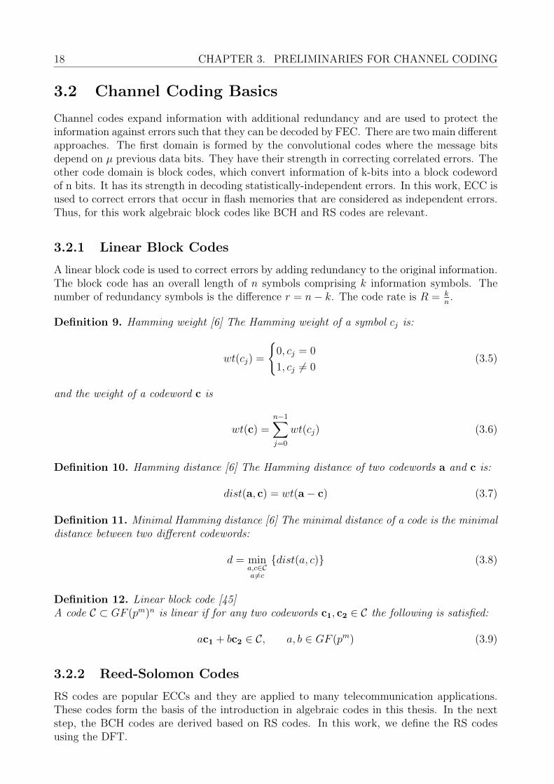
Definition 9. Hamming weight [6] The Hamming weight of a symbol cj is:
wt(cj) =
0, cj = 0
1, cj 6= 0(3.5)
and the weight of a codeword c is
wt(c) =n−1∑j=0
wt(cj) (3.6)
Definition 10. Hamming distance [6] The Hamming distance of two codewords a and c is:
dist(a, c) = wt(a− c) (3.7)
Definition 11. Minimal Hamming distance [6] The minimal distance of a code is the minimaldistance between two different codewords:
d = mina,c∈Ca6=c
dist(a, c) (3.8)
Definition 12. Linear block code [45]A code C ⊂ GF (pm)n is linear if for any two codewords c1, c2 ∈ C the following is satisfied:
ac1 + bc2 ∈ C, a, b ∈ GF (pm) (3.9)
3.2.2 Reed-Solomon Codes
RS codes are popular ECCs and they are applied to many telecommunication applications.These codes form the basis of the introduction in algebraic codes in this thesis. In the nextstep, the BCH codes are derived based on RS codes. In this work, we define the RS codesusing the DFT.
3.2. CHANNEL CODING BASICS 19
Definition 13. Reed-Solomon codes [6]Let α ∈ GF (pm) be an element of order n, then the RS code C is defined by the set ofpolynomials A(x) with a degree less than k : A(x) = A0 + A1x + A2x
2 + . . . + Ak−1xk−1, Ai ∈
GF (pm), k ≤ n.
C := a|ai = A(αi), i = 0, 1, . . . , n− 1, degree A(x) < k (3.10)
In definition 13, the RS code is defined using the DFT as F(a(x)) = A(x). Thisshows a relation between the codeword a = (a0, a1, . . . , an−1) and the information in A =(A0, A1, A2, . . . , Ak−1, 0, . . . , 0).
Alternatively, an information polynomial i(x) is encoded using the generator polynomialg(x) such that a(x) = i(x)g(x). The RS generator polynomial follows from definition 13 as:
g(x) =n−1∏j=k
(x− α−j) (3.11)
3.2.3 Bose-Chaudhuri-Hocquenghem Codes
We consider the binary BCH codes. It is convenient to represent the BCH codewords b asa codeword polynomial b(x). A BCH code can be either defined by the cyclotomic coset orsimilar to the RS code using the DFT.
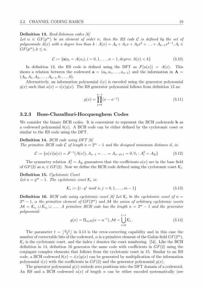
Definition 14. BCH code using DFT [6]The primitive BCH code C of length n = 2m − 1 and the designed minimum distance d, is:
C := a(x)|a(x) = F−1(A(x)), An−1 = . . . = An−d+1 = 0,∀i : A2i = A2i (3.12)
The symmetry relation A2i = A2i guarantees that the coefficients a(x) are in the base field
of GF (2) as ai ∈ GF (2). Now we define the BCH code defined using the cyclotomic coset Ki.
Definition 15. Cyclotomic CosetLet n = qm − 1. The cyclotomic coset Ki is:
Ki := i · qj mod n, j = 0, 1, . . . ,m− 1 (3.13)
Definition 16. BCH code using cyclotomic coset [6] Let Ki be the cyclotomic coset of n =2m − 1, α the primitive element of GF (2m) and M the union of arbitrary cyclotomic cosetsM = Ki1 ∪ Ki2 ∪ . . .. A primitive BCH code has the length n = 2m − 1 and the generatorpolynomial:
g(x) = Πi∈M(x− α−i),M =t−1⋃i=0
Ki . (3.14)
The parameter t = bd−12c in 3.14 is the error-correcting capability and in this case the
number of correctable bits of the codeword, α is a primitive element of the Galois field GF (2m),Ki is the cyclotomic coset, and the index i denotes the coset numbering [54]. Like the BCHdefinition in 14, definition 16 generates the same code with coefficients in GF (2) using theconjugate complex elements that follows from the cyclotomic coset in 15. Similar to an RScode, a BCH codeword b(x) = i(x)g(x) can be generated by multiplication of the informationpolynomial i(x) with the coefficients in GF (2) and the generator polynomial g(x).
The generator polynomial g(x) embeds zero positions into the DFT domain of a codeword.An RS and a BCH codeword u(x) of length n can be either encoded systematically (see
20 CHAPTER 3. PRELIMINARIES FOR CHANNEL CODING
Equation 3.15)), where the information i(x) with the length k itself is part of the codeword, ornon-systematically, where the original information has to be decoded to retrieve the originalinformation.
u(x) = i(x) · x(n−k) + i(x) · x(n−k) mod g(x) (3.15)
3.2.4 Algebraic Decoding
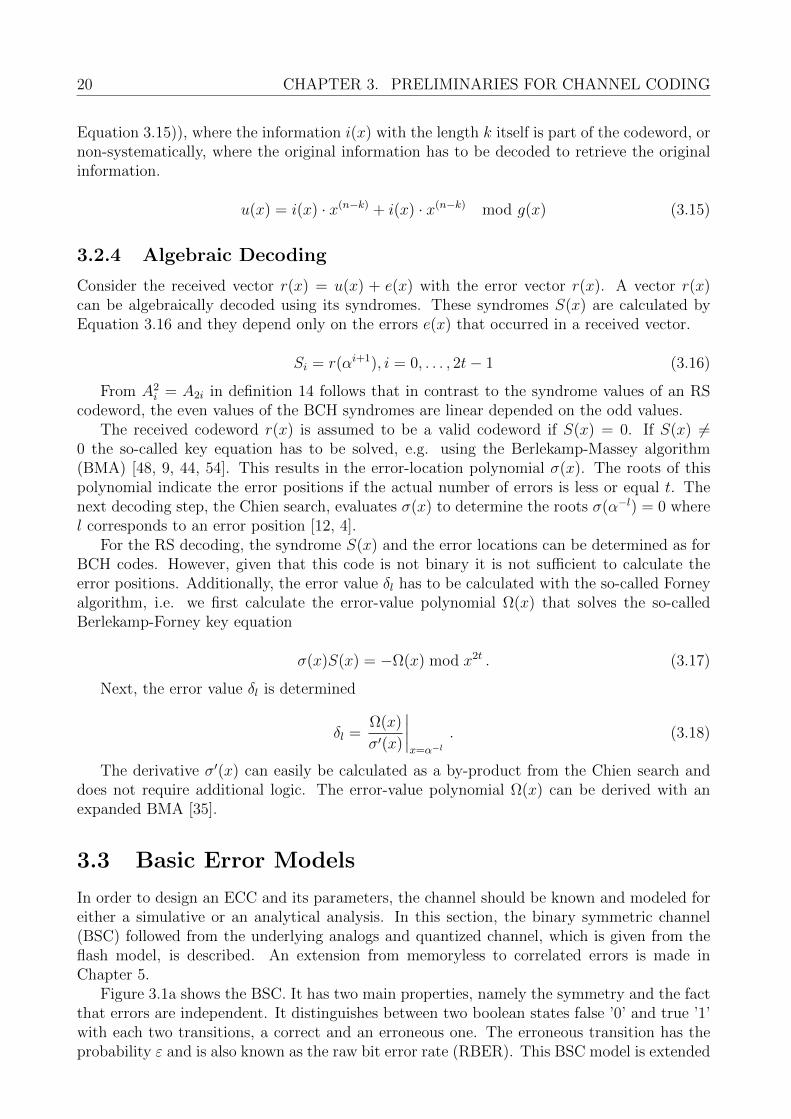
Consider the received vector r(x) = u(x) + e(x) with the error vector r(x). A vector r(x)can be algebraically decoded using its syndromes. These syndromes S(x) are calculated byEquation 3.16 and they depend only on the errors e(x) that occurred in a received vector.
Si = r(αi+1), i = 0, . . . , 2t− 1 (3.16)
From A2i = A2i in definition 14 follows that in contrast to the syndrome values of an RS
codeword, the even values of the BCH syndromes are linear depended on the odd values.The received codeword r(x) is assumed to be a valid codeword if S(x) = 0. If S(x) 6=
0 the so-called key equation has to be solved, e.g. using the Berlekamp-Massey algorithm(BMA) [48, 9, 44, 54]. This results in the error-location polynomial σ(x). The roots of thispolynomial indicate the error positions if the actual number of errors is less or equal t. Thenext decoding step, the Chien search, evaluates σ(x) to determine the roots σ(α−l) = 0 wherel corresponds to an error position [12, 4].
For the RS decoding, the syndrome S(x) and the error locations can be determined as forBCH codes. However, given that this code is not binary it is not sufficient to calculate theerror positions. Additionally, the error value δl has to be calculated with the so-called Forneyalgorithm, i.e. we first calculate the error-value polynomial Ω(x) that solves the so-calledBerlekamp-Forney key equation
σ(x)S(x) = −Ω(x) mod x2t . (3.17)
Next, the error value δl is determined
δl =Ω(x)
σ′(x)
∣∣∣∣x=α−l
. (3.18)
The derivative σ′(x) can easily be calculated as a by-product from the Chien search anddoes not require additional logic. The error-value polynomial Ω(x) can be derived with anexpanded BMA [35].
3.3 Basic Error Models
In order to design an ECC and its parameters, the channel should be known and modeled foreither a simulative or an analytical analysis. In this section, the binary symmetric channel(BSC) followed from the underlying analogs and quantized channel, which is given from theflash model, is described. An extension from memoryless to correlated errors is made inChapter 5.
Figure 3.1a shows the BSC. It has two main properties, namely the symmetry and the factthat errors are independent. It distinguishes between two boolean states false ’0’ and true ’1’with each two transitions, a correct and an erroneous one. The erroneous transition has theprobability ε and is also known as the raw bit error rate (RBER). This BSC model is extended
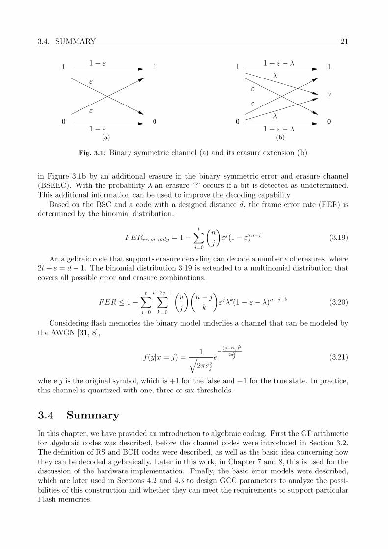
3.4. SUMMARY 21
1
0 0
11− ε
1− ε
ε
ε
?(a)
1
0 0
1
ε
ε
λ
λ
1− ε− λ
1− ε− λ
?
(b)
Fig. 3.1: Binary symmetric channel (a) and its erasure extension (b)
in Figure 3.1b by an additional erasure in the binary symmetric error and erasure channel(BSEEC). With the probability λ an erasure ’?’ occurs if a bit is detected as undetermined.This additional information can be used to improve the decoding capability.
Based on the BSC and a code with a designed distance d, the frame error rate (FER) isdetermined by the binomial distribution.
FERerror only = 1−t∑
j=0
(n
j
)εj(1− ε)n−j (3.19)
An algebraic code that supports erasure decoding can decode a number e of erasures, where2t+ e = d− 1. The binomial distribution 3.19 is extended to a multinomial distribution thatcovers all possible error and erasure combinations.
FER ≤ 1−t∑
j=0
d−2j−1∑k=0
(n
j
)(n− jk
)εjλk(1− ε− λ)n−j−k (3.20)
Considering flash memories the binary model underlies a channel that can be modeled bythe AWGN [31, 8],
f(y|x = j) =1√
2πσ2j
e−
(y−mj)2
2σ2j (3.21)
where j is the original symbol, which is +1 for the false and −1 for the true state. In practice,this channel is quantized with one, three or six thresholds.
3.4 Summary
In this chapter, we have provided an introduction to algebraic coding. First the GF arithmeticfor algebraic codes was described, before the channel codes were introduced in Section 3.2.The definition of RS and BCH codes were described, as well as the basic idea concerning howthey can be decoded algebraically. Later in this work, in Chapter 7 and 8, this is used for thediscussion of the hardware implementation. Finally, the basic error models were described,which are later used in Sections 4.2 and 4.3 to design GCC parameters to analyze the possi-bilities of this construction and whether they can meet the requirements to support particularFlash memories.
22
Chapter 4
Construction of high-rate GeneralizedConcatenated Codes for FlashMemories
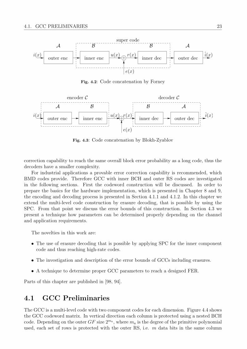
Code concatenation enables possibilities to combine codes with different characteristics. For-ney describes his view on concatenation first in [22]. This very intuitive view extends thechannel model shown in 4.1 with an additional outer encoder and decoder block as can beseen in Figure 4.2. The outer code considers the inner coder as a super channel. Thesame setup but with a different view is described by Blokh-Zyablov. They consider both in-ner and outer codes as a single code. This type of code concatenation is called generalizedconcatenated code (GCC).
A famous example for code concatenation is the DVB-T Standard. In its first version aninner convolution code is used which is concatenated with an outer RS code. The successorversion, DVB-T2 standard, uses an inner LDPC and outer BCH code. Each of these innercodes supports soft decision decoding like the Viterbi algorithm for the convolutional decodingand the belief propagation algorithm for the LDPC code. Soft decision decoding reaches ahigher gain than hard decision if the channel supports more than binary quantized values.In contrast to the convolutional code which produces in most error cases burst errors theLDPC code returns independent bit errors. The Reed Solomon code has good burst errorcorrection capabilities and thus it is used in combination with convolutional codes. TheBCH code has its advantages in independent error correction and is used in addition to theLDPC code as an outer code. RS and BCH codes have good error correction performancein hard decision decoding algorithms. Another famous combination of inner convolution andouter RS code is also used in the voyager program which started in 1977 [15] called Reed-Solomon/Viterbi (RSV).
One aspect of using concatenated codes in flash controllers is the fact that the componentcodes have small decoding complexity. The component codeword size is smaller and thusa smaller GF arithmetic is necessary. Furthermore, the component codes need less error
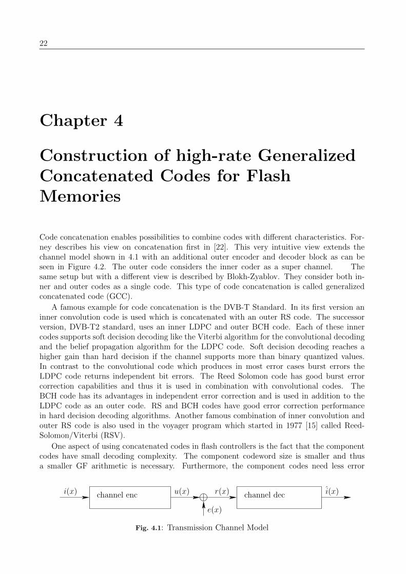
i(x) u(x)
e(x)
r(x) i(x)channel enc channel dec
Fig. 4.1: Transmission Channel Model
4.1. GCC PRELIMINARIES 23
i(x) u(x)
e(x)
r(x) i(x)
AA BB
inner encouter enc outer decinner dec
super code
C
Fig. 4.2: Code concatenation by Forney
i(x) u(x)
e(x)
r(x) i(x)
AA BB
inner encouter enc outer decinner dec
decoder Cencoder C
Fig. 4.3: Code concatenation by Blokh-Zyablov
correction capability to reach the same overall block error probability as a long code, thus thedecoders have a smaller complexity.
For industrial applications a provable error correction capability is recommended, whichBMD codes provide. Therefore GCC with inner BCH and outer RS codes are investigatedin the following sections. First the codeword construction will be discussed. In order toprepare the basics for the hardware implementation, which is presented in Chapter 8 and 9,the encoding and decoding process is presented in Section 4.1.1 and 4.1.2. In this chapter weextend the multi-level code construction by erasure decoding, that is possible by using theSPC. From that point we discuss the error bounds of this construction. In Section 4.3 wepresent a technique how parameters can be determined properly depending on the channeland application requirements.
The novelties in this work are:
• The use of erasure decoding that is possible by applying SPC for the inner componentcode and thus reaching high-rate codes.
• The investigation and description of the error bounds of GCCs including erasures.
• A technique to determine proper GCC parameters to reach a designed FER.
Parts of this chapter are published in [98, 94].
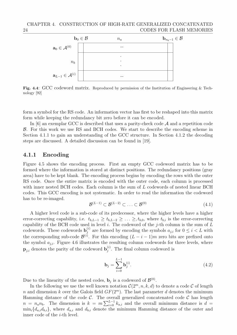
4.1 GCC Preliminaries
The GCC is a multi-level code with two component codes for each dimension. Figure 4.4 showsthe GCC codeword matrix. In vertical direction each column is protected using a nested BCHcode. Depending on the outer GF size 2ma , where ma is the degree of the primitive polynomialused, each set of rows is protected with the outer RS, i.e. m data bits in the same column
24CHAPTER 4. CONSTRUCTION OF HIGH-RATE GENERALIZED CONCATENATED
CODES FOR FLASH MEMORIES
.
.
.
...
...
b0 ∈ B bnb−1 ∈ B
nb
a0 ∈ A(0)
aL−1 ∈ A(i)
na
Fig. 4.4: GCC codeword matrix. Reproduced by permission of the Institution of Engineering & Tech-nology [92]
form a symbol for the RS code. An information vector has first to be reshaped into this matrixform while keeping the redundancy bit zero before it can be encoded.
In [6] an exemplar GCC is described that uses a parity-check code A and a repetition codeB. For this work we use RS and BCH codes. We start to describe the encoding scheme inSection 4.1.1 to gain an understanding of the GCC structure. In Section 4.1.2 the decodingsteps are discussed. A detailed discussion can be found in [19].
4.1.1 Encoding
Figure 4.5 shows the encoding process. First an empty GCC codeword matrix has to beformed where the information is stored at distinct positions. The redundancy positions (grayarea) have to be kept blank. The encoding process begins by encoding the rows with the outerRS code. Once the entire matrix is encoded with the outer code, each column is processedwith inner nested BCH codes. Each column is the sum of L codewords of nested linear BCHcodes. This GCC encoding is not systematic. In order to read the information the codewordhas to be re-imaged.
B(L−1) ⊂ B(L−2) ⊂ . . . ⊂ B(0) (4.1)
A higher level code is a sub-code of its predecessor, where the higher levels have a highererror-correcting capability, i.e. tb,L−1 ≥ tb,L−2 ≥ . . . ≥, tb,0, where tb,i is the error-correctingcapability of the BCH code used in level i. The codeword of the j-th column is the sum of Lcodewords. These codewords b
(i)j are formed by encoding the symbols aj,i for 0 ≤ i < L with
the corresponding sub-code B(i). For this encoding (L − i − 1)m zero bits are prefixed ontothe symbol aj,i. Figure 4.6 illustrates the resulting column codewords for three levels, where
pj,i denotes the parity of the codeword b(i)j . The final column codeword is
bj =L−1∑i=0
b(i)j . (4.2)
Due to the linearity of the nested codes, bj is a codeword of B(0).In the following we use the well known notation C(2m, n, k, d) to denote a code C of length
n and dimension k over the Galois field GF (2m). The last parameter d denotes the minimumHamming distance of the code C. The overall generalized concatenated code C has lengthn = nanb. The dimension is k = m
∑L−1i=0 ka,i and the overall minimum distance is d =
minida,idb,i, where da,i and db,i denote the minimum Hamming distance of the outer andinner code of the i-th level.

4.1. GCC PRELIMINARIES 25
outerencoding
innerencoding
with informationdata matrix
with outer codewordsdata matrix
GC codeword matrix
na
nb
mL
Fig. 4.5: GCC encoding
b(2)j ∈ B(2)
b(1)j ∈ B(1)
b(0)j ∈ B(0) 0
0
0
pj,2
pj,1
pj,0
aj,2
aj,1
aj,0
b(0)j + b
(1)j + b
(2)j = bj ∈ B(0)
Fig. 4.6: Nested BCH codeword. Reproduced by permission of the Institution of Engineering & Tech-nology [92]
26CHAPTER 4. CONSTRUCTION OF HIGH-RATE GENERALIZED CONCATENATED
CODES FOR FLASH MEMORIES
level j kb,j db,j ka,j da,j0 117 2 84 691 108 4 130 232 99 6 136 173 90 8 142 11
4-12 81 12 148 5
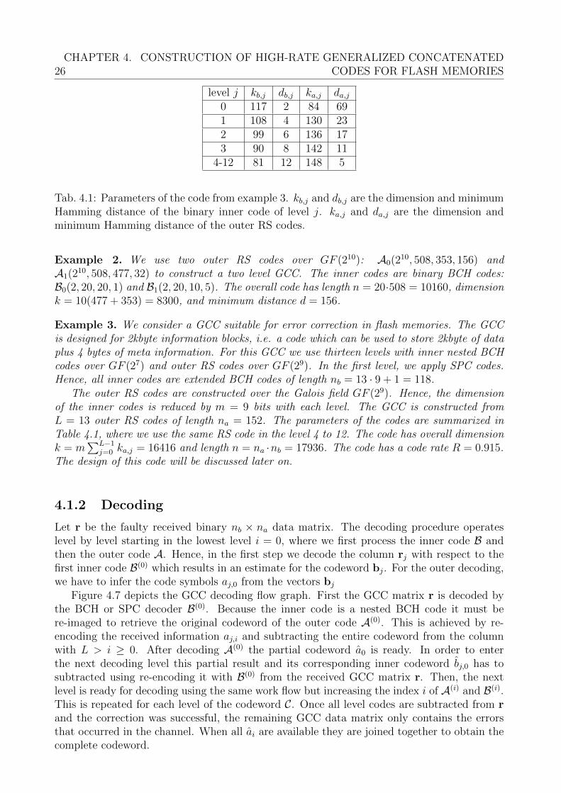
Tab. 4.1: Parameters of the code from example 3. kb,j and db,j are the dimension and minimumHamming distance of the binary inner code of level j. ka,j and da,j are the dimension andminimum Hamming distance of the outer RS codes.
Example 2. We use two outer RS codes over GF (210): A0(210, 508, 353, 156) andA1(210, 508, 477, 32) to construct a two level GCC. The inner codes are binary BCH codes:B0(2, 20, 20, 1) and B1(2, 20, 10, 5). The overall code has length n = 20·508 = 10160, dimensionk = 10(477 + 353) = 8300, and minimum distance d = 156.
Example 3. We consider a GCC suitable for error correction in flash memories. The GCCis designed for 2kbyte information blocks, i.e. a code which can be used to store 2kbyte of dataplus 4 bytes of meta information. For this GCC we use thirteen levels with inner nested BCHcodes over GF (27) and outer RS codes over GF (29). In the first level, we apply SPC codes.Hence, all inner codes are extended BCH codes of length nb = 13 · 9 + 1 = 118.
The outer RS codes are constructed over the Galois field GF (29). Hence, the dimensionof the inner codes is reduced by m = 9 bits with each level. The GCC is constructed fromL = 13 outer RS codes of length na = 152. The parameters of the codes are summarized inTable 4.1, where we use the same RS code in the level 4 to 12. The code has overall dimensionk = m
∑L−1j=0 ka,j = 16416 and length n = na ·nb = 17936. The code has a code rate R = 0.915.
The design of this code will be discussed later on.
4.1.2 Decoding
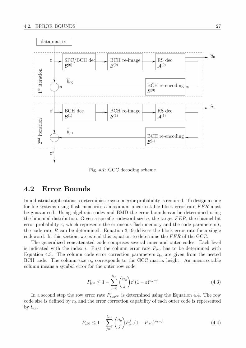
Let r be the faulty received binary nb × na data matrix. The decoding procedure operateslevel by level starting in the lowest level i = 0, where we first process the inner code B andthen the outer code A. Hence, in the first step we decode the column rj with respect to thefirst inner code B(0) which results in an estimate for the codeword bj. For the outer decoding,we have to infer the code symbols aj,0 from the vectors bj
Figure 4.7 depicts the GCC decoding flow graph. First the GCC matrix r is decoded bythe BCH or SPC decoder B(0). Because the inner code is a nested BCH code it must bere-imaged to retrieve the original codeword of the outer code A(0). This is achieved by re-encoding the received information aj,i and subtracting the entire codeword from the columnwith L > i ≥ 0. After decoding A(0) the partial codeword a0 is ready. In order to enterthe next decoding level this partial result and its corresponding inner codeword bj,0 has tosubtracted using re-encoding it with B(0) from the received GCC matrix r. Then, the nextlevel is ready for decoding using the same work flow but increasing the index i of A(i) and B(i).This is repeated for each level of the codeword C. Once all level codes are subtracted from rand the correction was successful, the remaining GCC data matrix only contains the errorsthat occurred in the channel. When all ai are available they are joined together to obtain thecomplete codeword.
4.2. ERROR BOUNDS 27
data matrix
BCH re-image
BCH re-image
BCH re-encoding
BCH re-encoding
1stiteration
2nditeration
r
r′
r′′
bj,0
bj,1
a0
a1
SPC/BCH dec
BCH dec
B(0)
B(0)B(0)
B(1)
B(1)B(1)
A(0)
A(1)RS dec
RS dec
Fig. 4.7: GCC decoding scheme
4.2 Error Bounds
In industrial applications a deterministic system error probability is required. To design a codefor file systems using flash memories a maximum uncorrectable block error rate FER mustbe guaranteed. Using algebraic codes and BMD the error bounds can be determined usingthe binomial distribution. Given a specific codeword size n, the target FER, the channel biterror probability ε, which represents the erroneous flash memory and the code parameters t,the code rate R can be determined. Equation 3.19 delivers the block error rate for a singlecodeword. In this section, we extend this equation to determine the FER of the GCC.
The generalized concatenated code comprises several inner and outer codes. Each levelis indicated with the index i. First the column error rate Pb(i) has to be determined withEquation 4.3. The column code error correction parameters tb,i are given from the nestedBCH code. The column size na corresponds to the GCC matrix height. An uncorrectablecolumn means a symbol error for the outer row code.
Pb(i) ≤ 1−tb,i∑j=0
(naj
)εj(1− ε)na−j (4.3)
In a second step the row error rate Prow(i) is determined using the Equation 4.4. The rowcode size is defined by nb and the error correction capability of each outer code is representedby ta,i.
Pa(i) ≤ 1−ta,i∑j=0
(nbj
)P j
b(i)(1− Pb(i))nb−j (4.4)
28CHAPTER 4. CONSTRUCTION OF HIGH-RATE GENERALIZED CONCATENATED
CODES FOR FLASH MEMORIES
In order to reach high-rate codes, erasure decoding in the RS decoder is used. Thus aparity-check code in the lowest level leads to an improvement. In this case, 4.4 has to beextended to calculate the erasure probability λb and the error probability Pb of the inner codeB separately. In the case that an SPC is used in level 0 an error occurs if the number of errorsis even, whereas an erasure is declared if the number of errors is odd. Hence, we can calculatethe error probability of the inner codes of the first level as
Pb(0) ≤nb∑
j=2,4,6,...
(nbj
)εj(1− ε)(nb−j) (4.5)
and
λb(0) ≤nb∑
j=1,3,5,...
(nbj
)εj(1− ε)(nb−j) . (4.6)
In general, a decoding error with inner decoding occurs only if the number of errors in thej-th column is greater or equal to tb,l + 2, whereas a decoding failure occurs for tb,l + 1 errors.Hence, we can bound the error and erasure probabilities for the inner code of the other levelsby
Pb(l) ≤nb∑
j=t+2
(nbj
)εj(1− ε)(nb−j) (4.7)
and
λb(l) ≤nb∑
j=t+1
(nbj
)εj(1− ε)(nb−j) . (4.8)
Thus we obtain an outer code error probability Pa,l per level l of
Pa(l) ≤ 1−ta,l∑j=0
da,l−2j−1∑k
(naj
)(na − jka
)P jb,lλ
kb,l(1− Pb,l − λb,l)(na−v−ka) . (4.9)
Finally the sum of all row error probabilities Prow(i) is the overall block error FER rate ofthe GCC codeword.
FER ≤L−1∑i=0
Pa(i) (4.10)
As already mentioned in practice ε, the codeword size and FER are given and the appro-priate parameters na, nb, ta,i and tb,i have to be found. The optimum parameters cannot bedetermined analytically. This means that a search algorithm is needed to solve this problem,which is presented in the next Section 4.3. First a target block size (e.g. 1k, 2k, 4k ...) ischosen. Based on this decision a combination consisting of number of levels and number ofcolumns must be selected. Depending on the number of columns the proper GF (2ma) size forthe outer code has to be selected such that nb ≤ 2mb−1 is true. Based on the number of levelsand the symbol size mb of the outer code, the column code size is mi = na. Starting withan R = 1 inner code each tb(i) is defined by the maximum ability of the nested BCH code.The outer code error correction capability tb,i has to be found such that each level reaches aProw(i) ≤ FER and the condition in Equation 4.10 is satisfied.
Iteration above ε shows the code rate characteristics of the GCC with the chosen para-meters Levels, outer GF size and the error correction capability of the first inner code ta,0.Adjustments can be made by changing the amount of LGCC and ta,0.
4.3. CODE PARAMETERS 29
The concatenation comprises several codes and thus it is possible to construct a code witha so-called unequal error protection like [34, 58] by adjusting the error correction capabilityof individual levels. Because the outer code has quantization steps in the error correctioncapability t it is likely to have not an optimal equal error protection.
4.3 Code Parameters
First of all, we want to define the requirements, which are given by the channel and the usecase of non-volatile Flash memory for industrial environments. These memories have a specificpage-size that determines together with the physical block size k the demands of a file system,the maximum size of the codeword n and its available space for redundancy r that defines alower bound of the code rate R. On the other hand, the property of the floating gates definesthe channel error probability ε that varies over the lifetime. Additionally, the application setsthe requirements for a maximum FER which we assume in this work to be FER ≤ 10−16 atthe specified end of lifetime (EOL) of a Flash memory. The task in this section is to find thecode parameters for a given codeword size and channel signal to noise ratio (SNR) that satisfythe designed FER and the code rate R boundaries.
The GCC comprises the two-dimensional codeword matrix that have the size na and nb.Its product forms the GCC codeword size n. A shorter column size nb leads to more columnsna. As the column sizes shrinks, the number of errors in this column also declines. In this case,the outer codeword size increases and thus the row code needs a higher codeword distance tomeet the FER condition that leads to a lower R.
An additional aspect of how to determine the column size is the error correction capabilityof the inner levels. This depends on the constructibility of inner algebraic codes becausethe column code is limited to nb ≤ 2mb − 1. For the different levels of l, we have l ·ma + r0
redundancy bits available. The cyclotomic cosets determine the error correction capability thatis achievable in the corresponding level l. Furthermore, the number of columns na determinesthe GF size ma of A. A larger na leads to a larger ma and thus the distance gap between theinner levels of B will increase.
We propose a search algorithm in 1. Given the parameters k, FER, ε, nb and db we candetermine R, na and da.
In case of soft-decoding, the block error Pb,l respectively erasure rate λb,l of those levels lthat are soft decoded have to be determined simulative and replaces the results of the binomialdistribution. Example measurements of different soft-decoding performances of inner codeswill be described in Chapter 6.
Because Algorithm 1 optimizes regarding R with a fixed codeword size, a plot over Es/N0
and R can be drawn as in Figure 4.8. This enables the comparison of the code rate efficiencyfor several codes. In this case, the comparison of soft and hard decoding. In the region0.91 ≤ R ≤ 0.95 the soft-decoding presented later leads to a gain of about 1dB.
Figure 4.9 shows a plot of the FER over Es/N0 for each level code Al. In this examplethe GCC code has twelve levels. In order to increase the decoding capability by using softdecoding, the first three hard decoding levels are replaced by a bit-flipping algorithm and theChase decoder, both will be described in Section 6.3. The overall GCC FER is the unionbound of all level codes Al, which corresponds to the envelope curves in Figure 4.9. In Figure4.9 the code parameters are optimized for FER = 10−16 in the soft-decoding mode. The curvehas a error floor like shape with a bend around the designed FER.
Example 4. The target FER is 10−16 at ε = 3.8 · 10−3. We use the Galois field
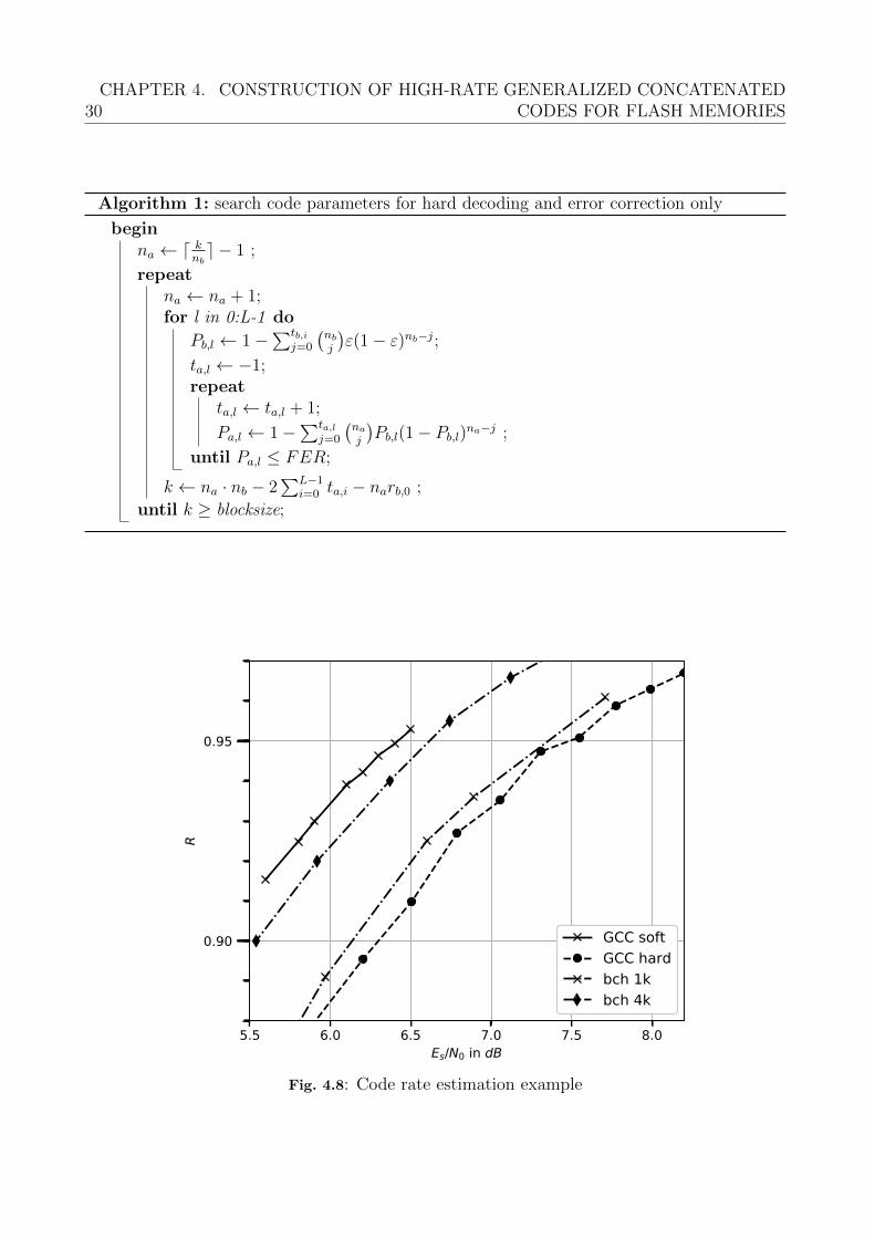
30CHAPTER 4. CONSTRUCTION OF HIGH-RATE GENERALIZED CONCATENATED
CODES FOR FLASH MEMORIES
Algorithm 1: search code parameters for hard decoding and error correction only
beginna ← d knb e − 1 ;
repeatna ← na + 1;for l in 0:L-1 do
Pb,l ← 1−∑tb,i
j=0
(nbj
)ε(1− ε)nb−j;
ta,l ← −1;repeat
ta,l ← ta,l + 1;
Pa,l ← 1−∑ta,l
j=0
(naj
)Pb,l(1− Pb,l)na−j ;
until Pa,l ≤ FER;
k ← na · nb − 2∑L−1
i=0 ta,i − narb,0 ;
until k ≥ blocksize;
5.5 6.0 6.5 7.0 7.5 8.0
Es/N0 in dB
0.90
0.95
R
GCC soft
GCC hard
bch 1k
bch 4k
decFig. 4.8: Code rate estimation example
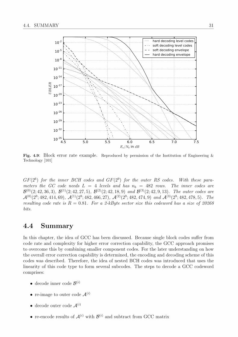
4.4. SUMMARY 31
4.5 5.0 5.5 6.0 6.5 7.0 7.5
Es/N0 in dB
10-35
10-32
10-29
10-26
10-23
10-20
10-17
10-14
10-11
10-8
10-5
10-2
UBLER
hard decoding level codes
soft decoding level codes
soft decoding envelope
hard decoding envelope
decFig. 4.9: Block error rate example. Reproduced by permission of the Institution of Engineering &Technology [101]
GF (26) for the inner BCH codes and GF (29) for the outer RS codes. With these para-meters the GC code needs L = 4 levels and has nb = 482 rows. The inner codes areB(0)(2; 42, 36, 3), B(1)(2; 42, 27, 5), B(2)(2; 42, 18, 9) and B(3)(2; 42, 9, 13). The outer codes areA(0)(29; 482, 414, 69), A(1)(29; 482, 466, 27), A(2)(29; 482, 474, 9) and A(3)(29; 482, 478, 5). Theresulting code rate is R = 0.81. For a 2-kByte sector size this codeword has a size of 20268bits.
4.4 Summary
In this chapter, the idea of GCC has been discussed. Because single block codes suffer fromcode rate and complexity for higher error correction capability, the GCC approach promisesto overcome this by combining smaller component codes. For the later understanding on howthe overall error correction capability is determined, the encoding and decoding scheme of thiscodes was described. Therefore, the idea of nested BCH codes was introduced that uses thelinearity of this code type to form several subcodes. The steps to decode a GCC codewordcomprises:
• decode inner code B(i)
• re-image to outer code A(i)
• decode outer code A(i)
• re-encode results of A(i) with B(i) and subtract from GCC matrix

32CHAPTER 4. CONSTRUCTION OF HIGH-RATE GENERALIZED CONCATENATED
CODES FOR FLASH MEMORIES
In principle the component codes of GCC are not necessary algebraic codes but the GCCwith algebraic codes enable an analytical error correction analysis based on the BMD propertyof its component codes, which is one of the important requirement of this work.
This GCC construction has the parameters:
• number of levels L
• GCC matrix dimension na and nb
• the GF field for the inner B and outer A component code
• error correction capabilities of each level for both component codes ta,l and tb,l
These parameters depend on each other and an optimal combination for a designed channelstate has to be searched e.g. with the proposed Algorithm 1 that still needs some manualintervention.
33
Chapter 5
Interleaver Construction Based onGaussian Integer
Codes over finite Gaussian integer fields were first studied by Huber in [33]. In this chapter setpartitioning of Gaussian integer constellations is considered. Set partitioning and multi-levelcoding is a common technique to combine coding and modulation. With this method thesignal constellation is split into subsets of equal size and the numbering of the subsets is thenencoded with different codes. For ordinary Gaussian integer fields, there exist no signal setpartitions, because the number of field elements is a prime. In [24, 23], it was demonstratedthat the concept of set partitioning can be applied to Gaussian integer rings of size m = c · d,where c and d are primes of the form c ≡ d ≡ 1 mod 4, respectively. This construction isbased on additive sub-groups of the ring constellation. Such constellations do not exist forintegers m that have any prime factor congruent to 3 modulo 4.
This work extends the results from [24, 23] to Gaussian integer constellations that areconstructed from the extension field GF (p2). In fact, the new construction is applicable forarbitrary integers p, therefore we consider two-dimensional Z-modules over integer rings Zp.The presented set partitioning is useful for the design of two-dimensional interleavers. Suchinterleavers can be utilized to correct clusters of errors, which occur for instance in magneticor optical storage systems.
In contrast to most publications on two-dimensional interleavers, we consider error clustersthat have a cyclic structure. Such interleavers may be useful for transmission with orthogonalfrequency-division multiplexing (OFDM) over frequency selective channels. The correspond-ing channel transfer functions typically lead to circularly correlated channel coefficients andtherefore cyclic error patterns [59]. To the best of our knowledge, similar error clusters and in-terleavers were only considered by De Almeida and Palazzo in [14], where the interleaving wasdesigned based on the set partitioning of a p×p array. The partitioning was obtained by opti-mizing the minimum squared Euclidean distance in the subsets. In this work, we demonstratethat the Mannheim metric is a suitable distance measure for the set partitioning of circularsquare arrays. Therefore, we propose a set partitioning based on the Mannheim metric. Theinterleaver design for square arrays presented in [5] is also based on the partitioning of lat-tices. This approach was later generalized to rectangular arrays [29]. However, the proposedpartitioning optimizes the Manhattan distance in the subsets, which does not regard cyclicstructures. Therefore, the construction in [5] cannot be directly applied to circular arrays.
Parts of this chapter are published in [86].
34 CHAPTER 5. INTERLEAVER CONSTRUCTION BASED ON GAUSSIAN INTEGER
5.1 Preliminaries
Gaussian integers are complex numbers such that the real and imaginary parts are integers.The modulo function of a complex number z is defined as
µ(z) = z mod λ = z −⌊zλ∗
λ · λ∗
⌉· λ, (5.1)
where λ∗ is the conjugate of the complex number λ. b·e denotes rounding to the closestGaussian integer, i.e. for a complex number z = a+ ib, we have bze = bae+ i bbe. Primes p ofthe form p ≡ 1 mod 4 can be decomposed into two complex numbers λ and λ∗, i.e. p = λ · λ∗.In this case, the complex modulo function is an operation-preserving isomorphism for thefinite integer field Zp = 0, 1, . . . , p− 1 and hence Gp = µ(z)|z ∈ Zp is also a finite fieldwith respect to complex addition and complex multiplication modulo λ.
In his seminal work [33], Huber presented Gaussian integer fields that are constructed fromextension fields GF (p2) for primes p of the form p ≡ 3 mod 4. For these constellations we usethe modulo function with λ = p. Hence, we have
µ(z) = z mod p = z −⌊z
p
⌉· p. (5.2)
The set Gp2 is obtained asGp2 = µ(k + i · l)|k, l ∈ Zp. (5.3)
We will also consider the case where p is not a prime and therefore Zp is a ring over integers.In this case, Gp2 is a module, which is a generalization of the notion of a vector space suchthat the scalars are the elements of an arbitrary ring.
The L1-norm (Manhattan norm) of a complex number z = a + ib is ||z|| = |a| + |b|. Wedefine the Mannheim weight of a Gaussian integer z by
wtM(z) = ||µ(z)||. (5.4)
The Mannheim distance between two Gaussian integers y and z is
dM(y, z) = wtM(y − z). (5.5)
Note that this definition coincides with the original definition introduced by Huber in [33].However, this definition of the Mannheim distance is not a proper distance for all possibleGaussian integer constellations, because the triangle inequality might not hold [47]. Thisissue occurs if there are Gaussian integers z with ||z|| < ||µ(z)||, i.e. the L1-norm of z issmaller than the norm of its representative in the finite set. In the following, we will showthat dM fulfills the metric axioms for Gaussian integer sets Gp2 as defined in Equation (5.3).
Lemma 1. For any module Gp2 with modulo function µ(·) and for any Gaussian integer z wehave
||µ(z)|| ≤ ||z||. (5.6)
Proof. Let a and b be the real part and the imaginary part of zp. Then, with (5.1) we have
µ(z)
p=z
p−⌊z
p
⌉= a− bae+ i(b− bbe).
5.2. SET PARTITIONING 35
Due to rounding we have |a− bae | ≤ |a| and |b− bbe | ≤ |b|. Consequently, we obtain
||µ(z)
p|| ≤ ||z
p|| = |a|+ |b|
and therefore ||µ(z)|| ≤ ||z||.
Theorem 1. The Mannheim distance dM defines a distance over Gp2.
Proof. Let a, b, c be three elements from Gp2 . We have to prove that the triangular inequalityis satisfied. Consider x = µ(a−c) and y = µ(c−b). We have µ(a−b) = µ(x+y) and thereforedM(a, b) = ||µ(a− b)|| = ||µ(x+ y)||. From Lemma 1 follows
||µ(x+ y)|| ≤ ||x+ y|| ≤ ||x||+ ||y||.
With dM(a, c) = ||x|| and dM(c, b) = ||y|| we obtain
dM(a, b) ≤ dM(a, c) + dM(c, b).
5.2 Set Partitioning
In the following, we will construct subsets of the module Gp2 , i.e. we partition Gp2 into p
disjoint subsets G(k)
p2 , k = 0, . . . , p − 1 with p elements. Each subset should have a largeminimum distance, where we consider the Mannheim distance as distance measure. We definethe minimum intra-partition distances ∆(k) of G(k)
p2 as
∆(k) = minx,y∈G(k)
p2,x 6=y
dM(x, y). (5.7)
The overall minimum Mannheim distance is the minimum of all intra-partition distances
∆ = mink=0,...,p−1
∆(k). (5.8)
For the minimum Mannheim distance we have the following sphere-packing bound.
Theorem 2. Let ∆ be the minimum Mannheim distance in any of p subsets G(k)
p2 with k =0, . . . , p− 1. The number of subsets p satisfies
p ≥
∆2+1
2for odd ∆
(∆−1)2+12
for even ∆(5.9)
Proof. Let ∆ be the minimum Mannheim distance in any subset G(k)
p2 . Now consider any set
of points (sphere) where every point has at most Mannheim distance t = b∆−12c to a center
point. All of these points belong to different subsets, because the distance between any twopoints in this sphere is smaller than ∆. Consequently, the number of subsets has to be greateror equal to the number of points in the sphere. We bound p by counting the number of points

36 CHAPTER 5. INTERLEAVER CONSTRUCTION BASED ON GAUSSIAN INTEGER
in a sphere of radius t. Note that there are at least 4j points with distance j to the center.Therefore, the total number of points in a sphere of radius t is
N ≥ 1 + 4t∑
j=1
j = 2t2 + 2t+ 1. (5.10)
If ∆ is odd, then t = b∆−12c = ∆−1
2. With p ≥ N we have
p ≥ 2t2 + 2t+ 1 = 2
(∆− 1
2
)2
+ 2
(∆− 1
2
)+ 1 =
∆2 + 1
2
Similarly, for even values of ∆ we have t = b∆−12c = ∆
2− 1 and
p ≥ 2t2 + 2t+ 1 =(∆− 1)2 + 1
2.
Note that the sphere-packing bound of Theorem 2 can be fulfilled with equality. Therefore,we define the notion of a perfect set partitioning in analogy to perfect error-correcting codes.
Definition 17. Let ∆ be the minimum Mannheim distance in any subset G(k)
p2 . This setpartitioning is perfect, if
∆ =√
2p− 1. (5.11)
Next, we construct set partitions with good minimum Mannheim distance. We first con-sider the case, where p is an arbitrary prime. Note that we can consider the extension fieldGF (p2) as a two-dimensional vector space (Euclidean geometry) over the base field Zp [42].The mapping µ(·) is operation-preserving with respect to addition and multiplication withelements from the base field. Therefore, Gp2 is also a two-dimensional Euclidean geometry.We will denote the corresponding base field by
Gp = µ(k)|k ∈ Zp. (5.12)
In the following we construct set partitions as lines (1-flats) in Gp2 . We use bold symbols todenote elements a ∈ Gp2 , i.e. points in the Euclidean geometry. Let a ∈ Gp2 be a non-zeropoint. Then, the p points µ(βa)|β ∈ Gp form a line that passes through the origin (the zeropoint). Let a0 and a be two linearly independent points in Gp2 , i.e. β0a0 + βa 6= 0 unlessβ0 = β = 0. Then, the p points µ(βa + a0)|β ∈ Gp form a line through the point a0.The two lines βa and βa + a0 are parallel lines, i.e. they have no common points. The setµ(βa + a0)|β ∈ Gp is a coset of µ(βa)|β ∈ Gp. For any line through the origin there arep − 1 parallel lines. We use this fact to form the partitions of the set Gp2 . Clearly choosingak = µ(k), k ∈ Zp as an element of the base field and a ∈ Gp2 with non-zero imaginary part, thetwo points ak, a are linearly independent. Hence, we obtain the p subsets for k = 0, . . . , p− 1
G(k)
p2 = µ(βa + ak)|β ∈ Gp (5.13)
Now, we consider the general case. If p is not a prime, then Gp is a ring and Gp2 is a module.In this case, Equation (5.13) defines a coset if the real part and imaginary part of a are nozero divisors.
We chose a = c + id to construct the set of parallel lines, where c, d ∈ N, c ≥ d are thetwo largest integers satisfying c2 + d2 ≤ p. This construction generates all perfect partitionswith respect to the minimum Mannheim distance. In order to prove this result we require thefollowing lemmas.
5.2. SET PARTITIONING 37
Lemma 2. Consider the partition of the module Gp2 into the p subsets G(0)
p2 , . . . ,G(p−1)
p2 . The
minimum intra-partition distances ∆(k) for k = 0, 1 . . . , p− 1 satisfy
∆(k) = minz∈G(0)
p2\0||z||. (5.14)
Proof. Consider two elements z 6= z′ from the same subset. With z′′ = µ(z−z′), the Mannheimdistance is
dM(z, z′) = ||µ(z− z′)|| = ||z′′||, z′′ 6= 0, z′′ ∈ G(0)
p2
Hence, we haveδ(k) = min
z,z′∈G(k)p2,z 6=z′
||z− z′||2 = minz′′∈G(0)
p2,z′′ 6=0
||z′′||2.
which holds for all parallel lines (cosets).
Next, we bound the minimum distance in the subsets of Gp2 . However, we consider onlyintegers p that satisfy the following Diophantine equation p = c2 + d2 for integers c and d.
Construction 1 Let p be an integer satisfying p = c2 + d2 with c, d ∈ N, where c and d arerelatively prime. Furthermore, neither c nor d is a zero divisor. We obtain the p subsets fork = 0, . . . , p− 1 according to Equation (5.13) with a = c+ id and ak = µ(k), k ∈ Zp.
Theorem 3. Consider the partition of the module Gp2 into the p subsets G(0)
p2 , . . . ,G(p−1)
p2 ac-cording to Construction 1. The minimum Mannheim distance ∆ satisfies
∆ ≥ c+ d. (5.15)
Proof. For integers of the form p = c2 + d2, p can be decomposed as p = λλ∗ with λ = c+ id,where λ is a Gaussian prime, because c and d are relatively prime. Now note that all elementsz ∈ G(0)
p2 \ 0 are multiples of λ = c+ id, i.e. z = β · λ with β ∈ Gp \ 0. Therefore, we have
µ(z) = βλ−⌊βλ
p
⌉p
= λ
(β −
⌊βλ
p
⌉λ∗)
= λ · A, withA =
(β −
⌊βλ
p
⌉λ∗).
Note that µ(z) 6= 0 implies that A is a non-zero Gaussian integer. Moreover, any non-zeroGaussian integer has a norm of at least one. Hence, we have
||µ(z)|| = ||λ|| · ||A|| ≥ ||λ|| = c+ d.
Using Lemma 2, we conclude that ∆ ≥ c+ d holds for all parallel lines.
Combining the results from Theorem 2 and Theorem 3, we note that the upper bound maycoincide with the lower bound.
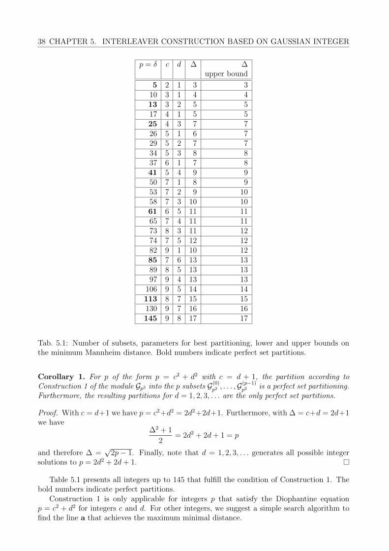
38 CHAPTER 5. INTERLEAVER CONSTRUCTION BASED ON GAUSSIAN INTEGER
p = δ c d ∆ ∆upper bound
5 2 1 3 310 3 1 4 413 3 2 5 517 4 1 5 525 4 3 7 726 5 1 6 729 5 2 7 734 5 3 8 837 6 1 7 841 5 4 9 950 7 1 8 953 7 2 9 1058 7 3 10 1061 6 5 11 1165 7 4 11 1173 8 3 11 1274 7 5 12 1282 9 1 10 1285 7 6 13 1389 8 5 13 1397 9 4 13 13
106 9 5 14 14113 8 7 15 15130 9 7 16 16145 9 8 17 17
Tab. 5.1: Number of subsets, parameters for best partitioning, lower and upper bounds onthe minimum Mannheim distance. Bold numbers indicate perfect set partitions.
Corollary 1. For p of the form p = c2 + d2 with c = d + 1, the partition according toConstruction 1 of the module Gp2 into the p subsets G(0)
p2 , . . . ,G(p−1)
p2 is a perfect set partitioning.Furthermore, the resulting partitions for d = 1, 2, 3, . . . are the only perfect set partitions.
Proof. With c = d+1 we have p = c2+d2 = 2d2+2d+1. Furthermore, with ∆ = c+d = 2d+1we have
∆2 + 1
2= 2d2 + 2d+ 1 = p
and therefore ∆ =√
2p− 1. Finally, note that d = 1, 2, 3, . . . generates all possible integersolutions to p = 2d2 + 2d+ 1.
Table 5.1 presents all integers up to 145 that fulfill the condition of Construction 1. Thebold numbers indicate perfect partitions.
Construction 1 is only applicable for integers p that satisfy the Diophantine equationp = c2 + d2 for integers c and d. For other integers, we suggest a simple search algorithm tofind the line a that achieves the maximum minimal distance.
5.3. INTERLEAVER DESIGN 39
Construction 2
1. Initialize ∆ = 0 and cmax = b√
2p− 1c+ 1
2. for c :=1 to cmax and for d := 1 to cmax repeat the following calculation:
– set a′ = c+ id
– construct the setG(0)
p2 = µ(βa′)|β ∈ Gp.
– determine∆′ = min
z∈G(0)p2\0||z||.
– if (∆′ > ∆) then set a = a′ and ∆ = ∆′.
The algorithm requires c2max ≈ 2p iterations. The construction of the set G(0)
p2 as well as thecalculation of the minimum norm require O(p) operations in standard O notation. Hence, thealgorithm has complexity O(p2). According to Lemma 2 the minimum distance is determined
by the norm of the elements of the set G(0)
p2 \ 0. In order to find the line a that achieves themaximum minimal distance in all subsets, it is sufficient to consider all values of c and d withc, d ∈ [1, cmax], because according to Theorem 2, the minimum Mannheim distance satisfies∆ ≤
√2p− 1 + 1.
5.3 Interleaver Design
An application of the presented set partitioning is the design of two-dimensional interleaversthat can be used to correct clusters of errors. Such errors occur in magnetic or optical storagesystems. We consider error clusters that have a square and possibly cyclic shape. Similarerror clusters and interleavers were presented by De Almeida and Palazzo in [14]. De Almeidaand Palazzo designed the interleaving based on the set partitioning of a p× p array. However,the partitioning is obtained by optimizing the minimum squared Euclidean distance in thesubsets. We will demonstrate that the cyclic error patterns considered by De Almeida andPalazzo can be characterized with the Mannheim distance. Therefore, we propose to use theMannheim distance for the design of the interleavers.
Figure 5.1 depicts 5 × 5 square arrays with two examples for two-dimensional clusters oferrors. In Figure 5.1 a) the center of the cluster lies in the center of the array. The clusterrepresents a sphere with radius one, i.e. all elements of the cluster have Mannheim distanceone to the center point. Similarly, Figure 5.1 b) depicts a cluster with a cyclic structure wherethe center point is in the right bottom corner of the square array. Again, the cluster representsa sphere with radius one with respect to the Mannheim distance.
The aim of the interleaving is to distribute all points in an error cluster to different rowsand columns of the array. Therefore, the errors can be corrected by applying error-correctingcodes to each row or column of the array. In order to design the interleaver, we consider theelements of the module Gp2 as indices of a p× p square array, i.e. the real part of z ∈ Gp2 canbe interpreted as column index and the imaginary part as row index. Hence, the interleaver isdefined by a bijective mapping Gp2 → Gp2 . To obtain an interleaving as depicted in Figure 5.1,all indices of one row of the array (all elements of Gp2 with the same imaginary part) shouldbe mapped to the same coset of Gp2 . Similarly all indices of one column of the array shouldbe mapped to the same coset of Gp2 . Such a mapping can be constructed as follows:
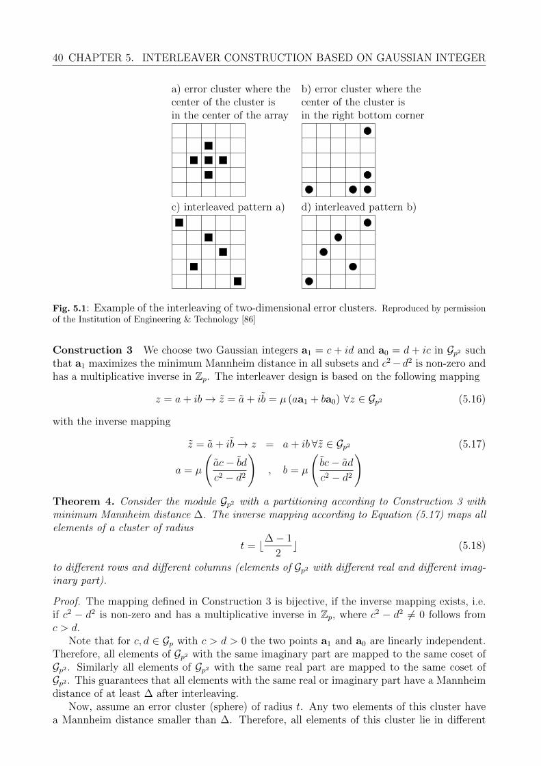
40 CHAPTER 5. INTERLEAVER CONSTRUCTION BASED ON GAUSSIAN INTEGER
a) error cluster where the b) error cluster where thecenter of the cluster is center of the cluster isin the center of the array in the right bottom corner
a,b a,b
c) interleaved pattern a) d) interleaved pattern b)
a,b a,b
Fig. 5.1: Example of the interleaving of two-dimensional error clusters. Reproduced by permissionof the Institution of Engineering & Technology [86]
Construction 3 We choose two Gaussian integers a1 = c + id and a0 = d + ic in Gp2 suchthat a1 maximizes the minimum Mannheim distance in all subsets and c2−d2 is non-zero andhas a multiplicative inverse in Zp. The interleaver design is based on the following mapping
z = a+ ib→ z = a+ ib = µ (aa1 + ba0) ∀z ∈ Gp2 (5.16)
with the inverse mapping
z = a+ ib→ z = a+ ib ∀z ∈ Gp2 (5.17)
a = µ
(ac− bdc2 − d2
), b = µ
(bc− adc2 − d2
)Theorem 4. Consider the module Gp2 with a partitioning according to Construction 3 withminimum Mannheim distance ∆. The inverse mapping according to Equation (5.17) maps allelements of a cluster of radius
t = b∆− 1
2c (5.18)
to different rows and different columns (elements of Gp2 with different real and different imag-inary part).
Proof. The mapping defined in Construction 3 is bijective, if the inverse mapping exists, i.e.if c2 − d2 is non-zero and has a multiplicative inverse in Zp, where c2 − d2 6= 0 follows fromc > d.
Note that for c, d ∈ Gp with c > d > 0 the two points a1 and a0 are linearly independent.Therefore, all elements of Gp2 with the same imaginary part are mapped to the same coset ofGp2 . Similarly all elements of Gp2 with the same real part are mapped to the same coset ofGp2 . This guarantees that all elements with the same real or imaginary part have a Mannheimdistance of at least ∆ after interleaving.
Now, assume an error cluster (sphere) of radius t. Any two elements of this cluster havea Mannheim distance smaller than ∆. Therefore, all elements of this cluster lie in different
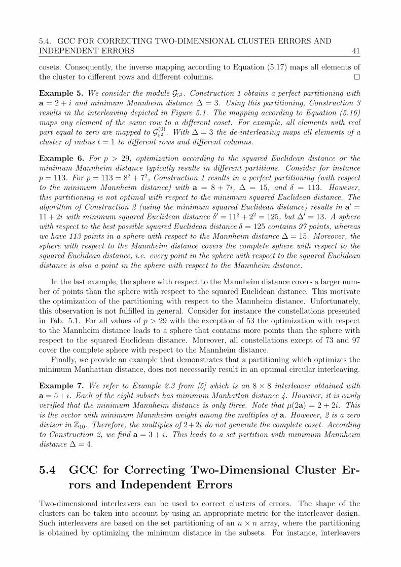
5.4. GCC FOR CORRECTING TWO-DIMENSIONAL CLUSTER ERRORS ANDINDEPENDENT ERRORS 41
cosets. Consequently, the inverse mapping according to Equation (5.17) maps all elements ofthe cluster to different rows and different columns.
Example 5. We consider the module G52. Construction 1 obtains a perfect partitioning witha = 2 + i and minimum Mannheim distance ∆ = 3. Using this partitioning, Construction 3results in the interleaving depicted in Figure 5.1. The mapping according to Equation (5.16)maps any element of the same row to a different coset. For example, all elements with realpart equal to zero are mapped to G(0)
52 . With ∆ = 3 the de-interleaving maps all elements of acluster of radius t = 1 to different rows and different columns.
Example 6. For p > 29, optimization according to the squared Euclidean distance or theminimum Mannheim distance typically results in different partitions. Consider for instancep = 113. For p = 113 = 82 + 72, Construction 1 results in a perfect partitioning (with respectto the minimum Mannheim distance) with a = 8 + 7i, ∆ = 15, and δ = 113. However,this partitioning is not optimal with respect to the minimum squared Euclidean distance. Thealgorithm of Construction 2 (using the minimum squared Euclidean distance) results in a′ =11 + 2i with minimum squared Euclidean distance δ′ = 112 + 22 = 125, but ∆′ = 13. A spherewith respect to the best possible squared Euclidean distance δ = 125 contains 97 points, whereaswe have 113 points in a sphere with respect to the Mannheim distance ∆ = 15. Moreover, thesphere with respect to the Mannheim distance covers the complete sphere with respect to thesquared Euclidean distance, i.e. every point in the sphere with respect to the squared Euclideandistance is also a point in the sphere with respect to the Mannheim distance.
In the last example, the sphere with respect to the Mannheim distance covers a larger num-ber of points than the sphere with respect to the squared Euclidean distance. This motivatethe optimization of the partitioning with respect to the Mannheim distance. Unfortunately,this observation is not fulfilled in general. Consider for instance the constellations presentedin Tab. 5.1. For all values of p > 29 with the exception of 53 the optimization with respectto the Mannheim distance leads to a sphere that contains more points than the sphere withrespect to the squared Euclidean distance. Moreover, all constellations except of 73 and 97cover the complete sphere with respect to the Mannheim distance.
Finally, we provide an example that demonstrates that a partitioning which optimizes theminimum Manhattan distance, does not necessarily result in an optimal circular interleaving.
Example 7. We refer to Example 2.3 from [5] which is an 8 × 8 interleaver obtained witha = 5 + i. Each of the eight subsets has minimum Manhattan distance 4. However, it is easilyverified that the minimum Mannheim distance is only three. Note that µ(2a) = 2 + 2i. Thisis the vector with minimum Mannheim weight among the multiples of a. However, 2 is a zerodivisor in Z10. Therefore, the multiples of 2+2i do not generate the complete coset. Accordingto Construction 2, we find a = 3 + i. This leads to a set partition with minimum Mannheimdistance ∆ = 4.
5.4 GCC for Correcting Two-Dimensional Cluster Er-
rors and Independent Errors
Two-dimensional interleavers can be used to correct clusters of errors. The shape of theclusters can be taken into account by using an appropriate metric for the interleaver design.Such interleavers are based on the set partitioning of an n × n array, where the partitioningis obtained by optimizing the minimum distance in the subsets. For instance, interleavers
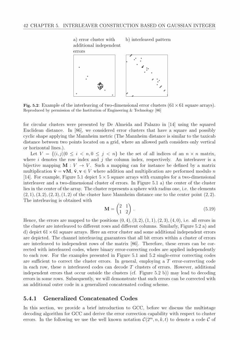
42 CHAPTER 5. INTERLEAVER CONSTRUCTION BASED ON GAUSSIAN INTEGER
a) error cluster with b) interleaved patternadditional independenterrors
a,b a,b
Fig. 5.2: Example of the interleaving of two-dimensional error clusters (61×61 square arrays).Reproduced by permission of the Institution of Engineering & Technology [86]
for circular clusters were presented by De Almeida and Palazzo in [14] using the squaredEuclidean distance. In [86], we considered error clusters that have a square and possiblycyclic shape applying the Mannheim metric (The Mannheim distance is similar to the taxicabdistance between two points located on a grid, where an allowed path considers only verticalor horizontal lines.).
Let V = (i, j)|0 ≤ i < n, 0 ≤ j < n be the set of all indices of an n × n matrix,where i denotes the row index and j the column index, respectively. An interleaver is abijective mapping M : V → V . Such a mapping can for instance be defined by a matrixmultiplication v = vM, v,v ∈ V where addition and multiplication are performed modulo n[14]. For example, Figure 5.1 depict 5× 5 square arrays with examples for a two-dimensionalinterleaver and a two-dimensional cluster of errors. In Figure 5.1 a) the center of the clusterlies in the center of the array. The cluster represents a sphere with radius one, i.e. the elements(2, 1), (3, 2), (2, 3), (1, 2) of the cluster have Mannheim distance one to the center point (2, 2).The interleaving is obtained with
M =
(2 11 2
). (5.19)
Hence, the errors are mapped to the positions (0, 4), (3, 2), (1, 1), (2, 3), (4, 0), i.e. all errors inthe cluster are interleaved to different rows and different columns. Similarly, Figure 5.2 a) andd) depict 61× 61 square arrays. Here an error cluster and some additional independent errorsare depicted. The channel interleaving guarantees that all bit errors within a cluster of errorsare interleaved to independent rows of the matrix [86]. Therefore, these errors can be cor-rected with interleaved codes, where binary error-correcting codes are applied independentlyto each row. For the examples presented in Figure 5.1 and 5.2 single-error correcting codesare sufficient to correct the cluster errors. In general, employing a T error-correcting codein each row, these n interleaved codes can decode T clusters of errors. However, additionalindependent errors that occur outside the clusters (cf. Figure 5.2 b)) may lead to decodingerrors in some rows. Subsequently, we will demonstrate that such errors can be corrected withan additional outer code in a generalized concatenated coding scheme.
5.4.1 Generalized Concatenated Codes
In this section, we provide a brief introduction to GCC, before we discuss the multistagedecoding algorithm for GCC and derive the error correction capability with respect to clustererrors. In the following we use the well known notation C(2m, n, k, t) to denote a code C of
5.4. GCC FOR CORRECTING TWO-DIMENSIONAL CLUSTER ERRORS ANDINDEPENDENT ERRORS 43
length n and dimension k over the Galois field GF (2m). The last parameter t denotes theerror-correcting capability of the code C.
In contrast to the GCC in Chapter 4, we do not necessarily use outer encoding in all levels.Therefore, we can also omit the restriction ki,l = lm. Note that an interleaved code is a specialcase of the GCC coding scheme, where we use no outer encoding and the information is encodedwith n parallel inner encoders for the same code B1(2, ni, ki, ti). Assuming proper interleaving,this interleaved code can correct ti error clusters. However, if ti error clusters occur, a singleindependent error may cause a decoding failure, because one row of the codeword matrix maycontain more than ti errors. Such an error event could be corrected with a single outer codewith to = 1. We demonstrate the basic concept with the following example.
Example 8. To construct a code for cluster error correction, we use binary BCH codes asinner codes: B(1)(2, 31, 26, 1) and B(2)(2, 31, 21, 2). However, we only use one outer RS codeover GF (25): A(1)(25, 31, 29, 1) to form five columns of the matrix. These five bits per row areencoded with the code B(1)(2, 31, 26, 1) where the remaining 21 = 26 - 5 bits are set to zero.The remaining 21 columns of the codeword matrix are filled with information bits without outerencoding. These information bits are encoded with the inner code B(2)(2, 31, 21, 2). Finally,the rows of the codeword matrix are obtained by adding all corresponding codewords from B(1)
and B(2). Due to B(2) ⊂ B(1), every row is a codeword of B(1). The overall code has length312 = 961, dimension k = 5 · 29 + 31 · 21 = 796 and requires only ten additional redundancybits compared to an interleaved code with B(1)(2, 31, 26, 1).
n = 31 is sufficiently large to interleave a cluster of radius 3 (cf. [86]). Such a clustercontains up to 25 bit errors. Hence, the code can correct any single-error cluster with at most25 bits. However, an additional independent error may cause a row in the codeword matrixwith two errors. Therefore, decoding of the corresponding row will lead to a decoding errorafter the inner decoding. Such a decoding error affects at most one symbol of the outer RScode. Hence, the outer code can be decoded correctly. Once, the code symbols of the outer codeare known, we can start a second round of inner decoding. In this decoding step we can usethe nested inner code B(2)(2, 31, 21, 2). Hence, the row containing two errors can be correctedin the second decoding round.
5.4.2 Code Constructions
Construction 1 We construct a GCC with L levels and with an n×n codeword matrix thatcorrects T clusters of errors and t ≤ L independent errors. For inner encoding we use the nestedbinary BCH codes B(L) ⊂ B(L−1) ⊂ . . . ⊂ B(1) of length n with ti,j = T + j − 1, j = 1, . . . , L.As outer codes we use RS codes with
to,j = b tjc. (5.20)
For interleaving we apply a two-dimensional channel interleaver as proposed in [86].
Theorem 5. The GCC according to Construction 1 corrects T clusters of errors and addi-tionally t independent bit errors.
Proof. The channel interleaving guarantees that all bit errors within a cluster of errors areinterleaved to independent rows of the codeword matrix [86]. Therefore T cluster errors causeat most T errors in each row of the codeword matrix. This T errors can be corrected in thefirst decoding round by the inner code B(1) if no additional errors occur.
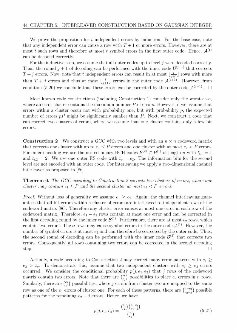
44 CHAPTER 5. INTERLEAVER CONSTRUCTION BASED ON GAUSSIAN INTEGER
We prove the proposition for t independent errors by induction. For the base case, notethat any independent error can cause a row with T + 1 or more errors. However, there are atmost t such rows and therefore at most t symbol errors in the first outer code. Hence, A(1)
can be decoded correctly.
For the inductive step, we assume that all outer codes up to level j were decoded correctly.Thus, the round j + 1 of decoding can be performed with the inner code B(j+1) that correctsT + j errors. Now, note that t independent errors can result in at most b t
j+1c rows with more
than T + j errors and thus at most b tj+1c errors in the outer code A(j+1). However, from
condition (5.20) we conclude that these errors can be corrected by the outer code A(j+1).
Most known code constructions (including Construction 1) consider only the worst case,where an error cluster contains the maximum number P of errors. However, if we assume thaterrors within a cluster occur not with probability one, but with probability p, the expectednumber of errors pP might be significantly smaller than P . Next, we construct a code thatcan correct two clusters of errors, where we assume that one cluster contains only a few biterrors.
Construction 2 We construct a GCC with two levels and with an n× n codeword matrixthat corrects one cluster with up to e1 ≤ P errors and one cluster with at most e2 < P errors.For inner encoding we use the nested binary BCH codes B(2) ⊂ B(1) of length n with ti,1 = 1and ti,2 = 2. We use one outer RS code with to = e2. The information bits for the secondlevel are not encoded with an outer code. For interleaving we apply a two-dimensional channelinterleaver as proposed in [86].
Theorem 6. The GCC according to Construction 2 corrects two clusters of errors, where onecluster may contain e1 ≤ P and the second cluster at most e2 < P errors.
Proof. Without loss of generality we assume e1 ≥ e2. Again, the channel interleaving guar-antees that all bit errors within a cluster of errors are interleaved to independent rows of thecodeword matrix [86]. Therefore any cluster error causes at most one error in each row of thecodeword matrix. Therefore, e1 − e2 rows contain at most one error and can be corrected inthe first decoding round by the inner code B(1). Furthermore, there are at most e2 rows, whichcontain two errors. These rows may cause symbol errors in the outer code A(1). However, thenumber of symbol errors is at most e2 and can therefore be corrected by the outer code. Thus,the second round of decoding can be performed with the inner code B(2) that corrects twoerrors. Consequently, all rows containing two errors can be corrected in the second decodingstep.
Actually, a code according to Construction 2 may correct many error patterns with e1 ≥e2 > to. To demonstrate this, assume that two independent clusters with e1 ≥ e2 errorsoccurred. We consider the conditional probability p(j, e1, e2) that j rows of the codewordmatrix contain two errors. Note that there are
(ne2
)possibilities to place e2 errors in n rows.
Similarly, there are(e1j
)possibilities, where j errors from cluster two are mapped to the same
row as one of the e1 errors of cluster one. For each of these patterns, there are(n−e1e2−j
)possible
patterns for the remaining e2 − j errors. Hence, we have
p(j, e1, e2) =
(e1j
)(n−e1e2−j
)(ne2
) (5.21)
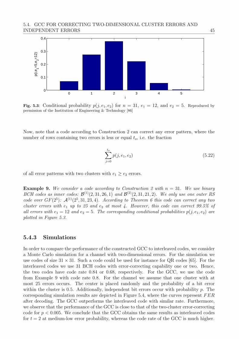
5.4. GCC FOR CORRECTING TWO-DIMENSIONAL CLUSTER ERRORS ANDINDEPENDENT ERRORS 45
0 1 2 3 4 50
0.1
0.2
0.3
0.4
i
p(i,e
1=5,
e 2=12
)
a,b
Fig. 5.3: Conditional probability p(j, e1, e2) for n = 31, e1 = 12, and e2 = 5. Reproduced bypermission of the Institution of Engineering & Technology [86]
Now, note that a code according to Construction 2 can correct any error pattern, where thenumber of rows containing two errors is less or equal to, i.e. the fraction
to∑j=0
p(j, e1, e2) (5.22)
of all error patterns with two clusters with e1 ≥ e2 errors.
Example 9. We consider a code according to Construction 2 with n = 31. We use binaryBCH codes as inner codes: B(1)(2, 31, 26, 1) and B(2)(2, 31, 21, 2). We only use one outer RScode over GF (25): A(1)(25, 31, 23, 4). According to Theorem 6 this code can correct any twocluster errors with e1 up to 25 and e2 at most 4. However, this code can correct 99.5% ofall errors with e1 = 12 and e2 = 5. The corresponding conditional probabilities p(j, e1, e2) areplotted in Figure 5.3.
5.4.3 Simulations
In order to compare the performance of the constructed GCC to interleaved codes, we considera Monte Carlo simulation for a channel with two-dimensional errors. For the simulation weuse codes of size 31 × 31. Such a code could be used for instance for QR codes [65]. For theinterleaved codes we use 31 BCH codes with error-correcting capability one or two. Hence,the two codes have code rate 0.84 or 0.68, respectively. For the GCC, we use the codefrom Example 9 with code rate 0.8. For the channel we assume that one cluster with atmost 25 errors occurs. The center is placed randomly and the probability of a bit errorwithin the cluster is 0.5. Additionally, independent bit errors occur with probability p. Thecorresponding simulation results are depicted in Figure 5.4, where the curves represent FERafter decoding. The GCC outperforms the interleaved code with similar rate. Furthermore,we observe that the performance of the GCC is close to that of the two-cluster error-correctingcode for p < 0.005. We conclude that the GCC obtains the same results as interleaved codesfor t = 2 at medium-low error probability, whereas the code rate of the GCC is much higher.
46 CHAPTER 5. INTERLEAVER CONSTRUCTION BASED ON GAUSSIAN INTEGER
0 0.005 0.01 0.015 0.02 0.025 0.0310
−3
10−2
10−1
100
p
WE
R
interleaved code, t=1GCCinterleaved code, t=2
a,b
Fig. 5.4: Simulation results for interleaved codes and the GCC of Example 9 for a channelthat produces one cluster of errors and independent errors with probability p. Reproduced bypermission of the Institution of Engineering & Technology [86]

5.5. CONCLUSIONS 47
5.5 Conclusions
In this chapter, we have introduced the concept of partitioning of Gaussian integer modulesGp2 . We have shown that Huber’s original definition of the Mannheim metric satisfies thedistance axioms over the considered class of Gaussian integers. Furthermore, we have derivedupper bounds on the minimum distance for the set partitioning. Next we have presentedtwo constructions for the set partitioning. Both constructions achieve optimum or close tooptimum set partitions. In particular, we have demonstrated that perfect set partitions withrespect to the sphere packing bound are attainable. This set partitioning enables multi-levelcode constructions over Gaussian integers. Furthermore, we have demonstrated that this setpartitioning can be applied to an interleaving technique for correcting two-dimensional cyclicclusters of errors.
48
Chapter 6
Soft-Decoding for GeneralizedConcatenated Codes
In this chapter, we describe soft-decoding techniques for the GCC. This promises an increaseof the error correction capability by considering more channel information using a quantizedinformation of an FG as described in Section 2.2.1. In [21], the author stated that it isin principle possible to extend the inner algebraic decoder of the GCC decoder by a morecomplex decoding algorithm employing soft-decoding. The soft-decoding algorithms leadto increased complexity. For instance, the trellis representation requires for a block codeO(2min[Rn,(1−R)n]) states and thus the memory complexity growths exponentially with the errorcorrection capability. Nevertheless, in the literature exists a large variety of soft-decodingalgorithms. In this chapter the stack algorithm and Chase decoding algorithm are presentedand investigated for their application in GCC and Flash memories. For the stack algorithm,or also called sequential decoder, we propose a less complex supercode decoding algorithmand show its relation to the subcodes of the nested BCH codes.
The novelties in this chapter are:
• Sequential stack decoding of nested BCH codes using supercodes [96].
• Applying different soft-decoding algorithms to decode the inner block codes in the GCC.
6.1 Sequential Stack Decoding
In this section, we describe sequential decoding procedures using the stack algorithm for blockcodes. These decoding methods are used to decode the binary inner codes. In Section 6.1.2 thesupercode decoding is introduced that reduces the trellis and thus the decoding complexity.
6.1.1 Sequential Stack Decoding using a Single Trellis
First, we consider the sequential decoding procedure as presented in [2]. All algorithms con-sidered in this section are based on this decoding method which uses a trellis to represent thecode. Later on, we will present improvements to this decoding algorithm.
The stack decoding procedure uses the trellis representation. A trellis T = (S,W) isa labeled, directed graph, where W = w denotes the set of all branches in the graphand S = σ is the set of all nodes. The set S is decomposed into n + 1 disjoint subsetsS = S0 ∪ S1 ∪ . . . ∪ Sn that are called levels of the trellis. Similarly, there exists a partition
6.1. SEQUENTIAL STACK DECODING 49
of the set W = W1 ∪ W2 ∪ . . . ∪ Wn. A node σ ∈ St of the level t may be connected witha node σ ∈ St+1 of the level t + 1 by one or several branches. Each branch wt is directedfrom a node σ of level t − 1 to a node σ of the next level t. We assume that the end levelshave only one node, namely S0 = σ0 and Sn = σn. A trellis is a compact methodof presenting all codewords of a code. Each branch of the trellis wt is labeled by a codesymbol vt(wt). Each distinct codeword corresponds to a distinct path in the trellis, i.e. thereis a one-to-one correspondence between each codeword v in the code and a path w in thetrellis: v(w) = v1(w1), . . . , vn(wn). We denote code sequence segments and path segments byv[i,j] = vi, . . . , vj and w[i,j] = wi, . . . , wj, respectively. The syndrome trellis, can be obtainedusing its parity-check matrix [70]. The syndrome trellis is minimal inasmuch as this trellishas the minimal possible number of nodes |S| among all possible trellis representations of thesame code.
The sequential decoding procedure as presented in [2] is a stack algorithm, i.e. a stack isrequired to store interim results. The stack contains code sequences of different lengths. Letvt denote a code sequence of length t, i.e. vt = v1, . . . , vt. Each code sequence is associatedwith a metric and a node σt. The node σt is the node in the trellis that is reached if we followthe path corresponding to the code sequence through the trellis. The metric rates each codesequence and the stack is ordered according to these metric values where the code sequence atthe top of the stack is the one with the largest metric value. There exist different metrics inthe literature to compare code sequences of different length. In the following, we consider theFano metric which is defined as follows. Let vi be the i-th code bit and ri the i-th receivedsymbol for transmission over a discrete memoryless channel. The Fano metric for a code bitvi is defined by
M(ri|vi) = log2
p(ri|vi)p(ri)
−B (6.1)
where p(ri|vi) is the channel transition probability and p(ri) is the probability to observe riat the channel output. The term B is a bias term that is typically chosen to be the code rateR [49]. The Fano metric of a code sequence vt is
M(rt|vt) =t∑i=1
M(ri|vi) (6.2)
where rt is the sequence of the first t received symbols. Note that the Fano metric accordingto Equation (6.1) is only defined for discrete memoryless channels (DMC). We consider thequantized AWGN channel which is a DMC. Binary block codes typically have no tree structure.Consequently, the Fano metric is not necessarily the best metric for all binary block codes.For instance, in [62] a metric with variable bias term was proposed for linear block codes.However, in our simulations for binary BCH codes we found that B = R provides good resultsfor all considered channel conditions.
We demonstrate Algorithm 2 in the following example, where for simplicity we assumetransmission over a binary symmetrical channel.
Example 10. Consider for instance the code B = (0000), (1110), (1011), (0101) with parity-check matrix
H =
(1 1 0 10 1 1 1
).
The corresponding trellis is depicted in Figure 6.1a). We assume transmission over a binarysymmetrical channel with error probability 0.1. Hence, we have
M(ri|vi) ≈
0.3 for ri = vi−2.8 for ri 6= vi
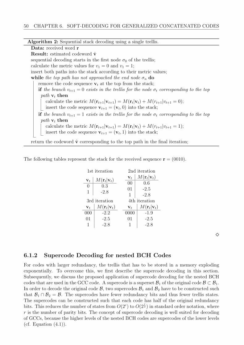
50 CHAPTER 6. SOFT-DECODING FOR GENERALIZED CONCATENATED CODES
Algorithm 2: Sequential stack decoding using a single trellis.
Data: received word rResult: estimated codeword vsequential decoding starts in the first node σ0 of the trellis;calculate the metric values for v1 = 0 and v1 = 1;insert both paths into the stack according to their metric values;while the top path has not approached the end node σn do
remove the code sequence vt at the top from the stack;if the branch vt+1 = 0 exists in the trellis for the node σt corresponding to the toppath vt then
calculate the metric M(rt+1|vt+1) = M(rt|vt) +M(rt+1|vt+1 = 0);insert the code sequence vt+1 = (vt, 0) into the stack;
if the branch vt+1 = 1 exists in the trellis for the node σt corresponding to the toppath vt then
calculate the metric M(rt+1|vt+1) = M(rt|vt) +M(rt+1|vt+1 = 1);insert the code sequence vt+1 = (vt, 1) into the stack;
return the codeword v corresponding to the top path in the final iteration;
The following tables represent the stack for the received sequence r = (0010).
1st iteration 2nd iteration
vt M(rt|vt)0 0.31 -2.8
vt M(rt|vt)00 0.601 -2.51 -2.8
3rd iteration 4th iterationvt M(rt|vt)
000 -2.201 -2.51 -2.8
vt M(rt|vt)0000 -1.901 -2.51 -2.8
6.1.2 Supercode Decoding for nested BCH Codes
For codes with larger redundancy, the trellis that has to be stored in a memory explodingexponentially. To overcome this, we first describe the supercode decoding in this section.Subsequently, we discuss the proposed application of supercode decoding for the nested BCHcodes that are used in the GCC code. A supercode is a superset B1 of the original code B ⊂ B1.In order to decode the original code B, two supercodes B1 and B2 have to be constructed suchthat B1 ∩ B2 = B. The supercodes have fewer redundancy bits and thus fewer trellis states.The supercodes can be constructed such that each code has half of the original redundancybits. This reduces the number of states from O(2r) to O(2
r2 ) in standard order notation, where
r is the number of parity bits. The concept of supercode decoding is well suited for decodingof GCCs, because the higher levels of the nested BCH codes are supercodes of the lower levels(cf. Equation (4.1)).
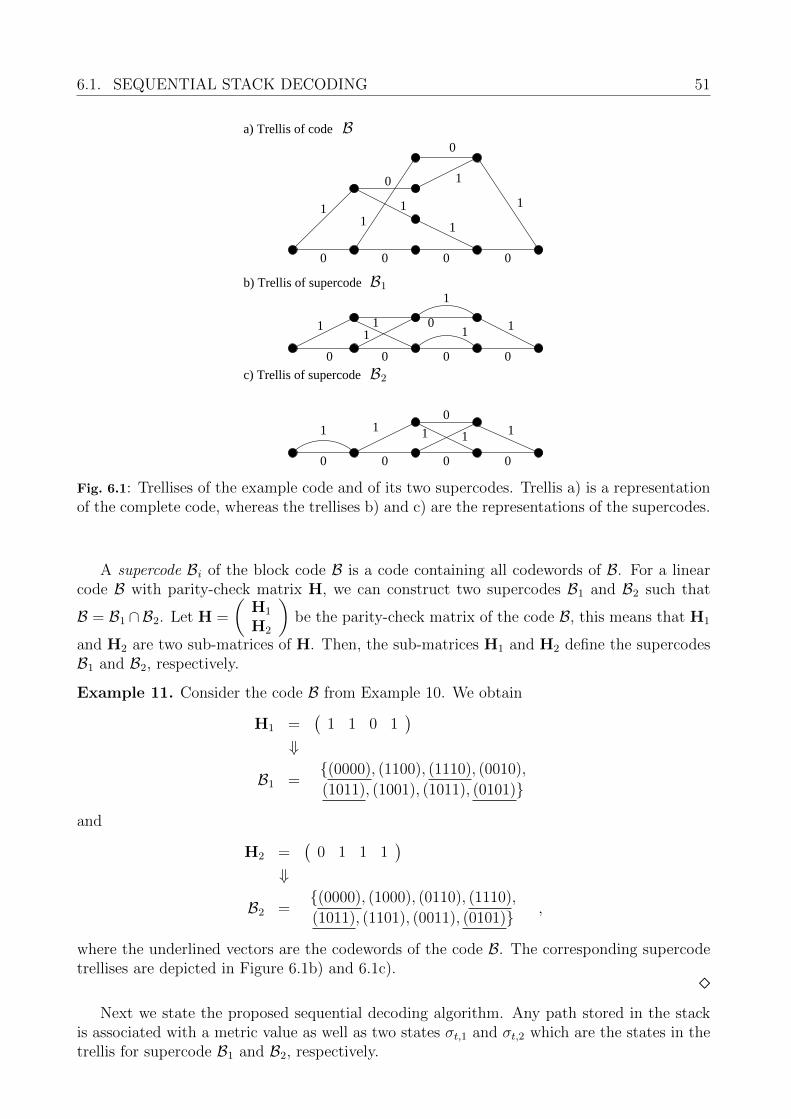
6.1. SEQUENTIAL STACK DECODING 51
1 110
1 1
c) Trellis of supercode
b) Trellis of supercode
0 0 00
0 0 00
0 0 0
1
1
11
101
0
1
1
11
1
1
0
0
a) Trellis of codeB
B1
B2
Fig. 6.1: Trellises of the example code and of its two supercodes. Trellis a) is a representationof the complete code, whereas the trellises b) and c) are the representations of the supercodes.
A supercode Bi of the block code B is a code containing all codewords of B. For a linearcode B with parity-check matrix H, we can construct two supercodes B1 and B2 such that
B = B1 ∩B2. Let H =
(H1
H2
)be the parity-check matrix of the code B, this means that H1
and H2 are two sub-matrices of H. Then, the sub-matrices H1 and H2 define the supercodesB1 and B2, respectively.
Example 11. Consider the code B from Example 10. We obtain
H1 =(
1 1 0 1)
⇓
B1 =(0000), (1100), (1110), (0010),
(1011), (1001), (1011), (0101)
and
H2 =(
0 1 1 1)
⇓
B2 =(0000), (1000), (0110), (1110),
(1011), (1101), (0011), (0101) ,
where the underlined vectors are the codewords of the code B. The corresponding supercodetrellises are depicted in Figure 6.1b) and 6.1c).
Next we state the proposed sequential decoding algorithm. Any path stored in the stack
is associated with a metric value as well as two states σt,1 and σt,2 which are the states in thetrellis for supercode B1 and B2, respectively.
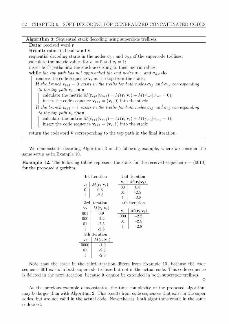
52 CHAPTER 6. SOFT-DECODING FOR GENERALIZED CONCATENATED CODES
Algorithm 3: Sequential stack decoding using supercode trellises.
Data: received word rResult: estimated codeword vsequential decoding starts in the nodes σ0,1 and σ0,2 of the supercode trellises;calculate the metric values for v1 = 0 and v1 = 1;insert both paths into the stack according to their metric values;while the top path has not approached the end nodes σn,1 and σn,2 do
remove the code sequence vt at the top from the stack;if the branch vt+1 = 0 exists in the trellis for both nodes σt,1 and σt,2 correspondingto the top path vt then
calculate the metric M(rt+1|vt+1) = M(rt|vt) +M(rt+1|vt+1 = 0);insert the code sequence vt+1 = (vt, 0) into the stack;
if the branch vt+1 = 1 exists in the trellis for both nodes σt,1 and σt,2 correspondingto the top path vt then
calculate the metric M(rt+1|vt+1) = M(rt|vt) +M(rt+1|vt+1 = 1);insert the code sequence vt+1 = (vt, 1) into the stack;
return the codeword v corresponding to the top path in the final iteration;
We demonstrate decoding Algorithm 3 in the following example, where we consider thesame setup as in Example 10.
Example 12. The following tables represent the stack for the received sequence r = (0010)for the proposed algorithm.
1st iteration 2nd iteration
vt M(rt|vt)0 0.31 -2.8
vt M(rt|vt)00 0.601 -2.51 -2.8
3rd iteration 4th iterationvt M(rt|vt)001 0.9000 -2.201 -2.51 -2.8
vt M(rt|vt)000 -2.201 -2.51 -2.8
5th iterationvt M(rt|vt)
0000 -1.901 -2.51 -2.8
Note that the stack in the third iteration differs from Example 10, because the codesequence 001 exists in both supercode trellises but not in the actual code. This code sequenceis deleted in the next iteration, because it cannot be extended in both supercode trellises.
As the previous example demonstrates, the time complexity of the proposed algorithmmay be larger than with Algorithm 2. This results from code sequences that exist in the supercodes, but are not valid in the actual code. Nevertheless, both algorithms result in the samecodeword.
6.1. SEQUENTIAL STACK DECODING 53
Theorem 7. Algorithm 2 and Algorithm 3 result in the same estimated codeword.
Proof. Both algorithms differ only with respect to the representation of the code. To prove theproposition it is sufficient to verify that both representations are equivalent. We first prove byinduction that the estimated codeword corresponds to a valid path in both supercode trellises,i.e. it is a codeword in both supercodes. The base case is the initial step where the codebits 0 and 1 are inserted in the stack. Note that a linear code has no code bit positions withconstant values. Hence, the transitions v1 = 0 and v1 = 1 exist in both supercode trellises. Forthe inductive step, we assume that a path for the code sequence vt exists in both supercodetrellises. It follows from Algorithm 2 that this path is only extended if the extended path existsin both supercode trellises. This proves the claim that the estimated codeword correspondsto a valid path in both supercode trellises. Now note that B = B1 ∩ B2, i.e. a path is onlyvalid in both supercode trellises if and only if it is a valid codeword of the code B.
Algorithm 3 reduces the space complexity required for representing the code. We demon-strate this in the following example.
Example 13. We consider three BCH codes from Table 4.1. All codes have length n = 60.In the first level, we use a single-error correcting code. This code has 3,262 nodes in the trellisand is a supercode of the BCH code of the second level. The trellis of the second level has159,742 nodes. However, utilizing the trellis of the first level code, we require only a singleadditional supercode trellis with 2,884 nodes to represent the code at the second level. Finally,the code at the third level has a trellis with 7,079,886 nodes. Using supercode decoding, weutilize the trellises of the first and second level and require one additional supercode trelliswith 2,410 nodes to represent the third code.
With sequential decoding the number of visited nodes in the trellis (the number of itera-tions) depends on the number of transmission errors. Note that with the presented codes thetime complexity with Algorithm 3 is at most 1.75 times larger than with Algorithm 2.
6.1.3 List-of-two Decoding
Next, we present two techniques to improve the performance and the complexity of Algo-rithm 2. First, we demonstrate that the soft-input decoding can be omitted in cases wherethe hard decision of the received vector corresponds to a valid codeword. Moreover, we pro-pose a sequential list-of-two decoding algorithm. List-of-two decoding is motivated by the factthat Algorithm 2 is not a maximum-likelihood decoding procedure. Hence, we may search forfurther codewords to find better candidates than the result of Algorithm 2.
Consider an additive white Gaussian noise channel with binary phase shift keying. A binarycode symbol vt ∈ F2 is mapped to the transmission symbol xt ∈ +1,−1 by xt = 1−2vt. Thetransmitted symbol vector x is distorted by a noise vector n such that the received sequenceis r = x + n. The noise vector n is a vector of independent identically distributed Gaussianrandom variables with mean zero. Hence,
p(rt | xt = ±1) =1√
2πσ2· e−
(rt∓1)2
2σ2 , (6.3)
where σ2 denotes the variance of the Gaussian distribution. For this channel, it is commonpractice to use the quadratic Euclidean distance d2
E(x, r) =∑n
t=1 |xt − rt|2 as metric, because
arg
(maxv∈C
P (r|v)
)= arg
(minv∈C
d2E(x, r)
). (6.4)
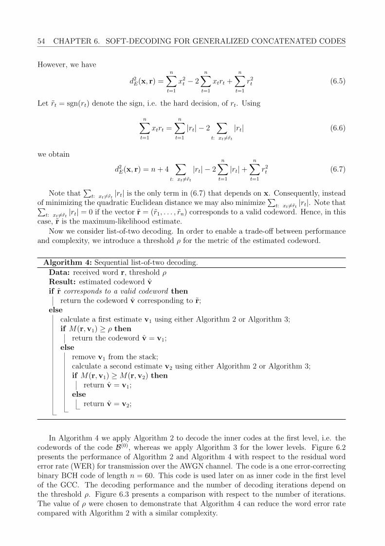
54 CHAPTER 6. SOFT-DECODING FOR GENERALIZED CONCATENATED CODES
However, we have
d2E(x, r) =
n∑t=1
x2t − 2
n∑t=1
xtrt +n∑t=1
r2t (6.5)
Let rt = sgn(rt) denote the sign, i.e. the hard decision, of rt. Using
n∑t=1
xtrt =n∑t=1
|rt| − 2∑
t: xt 6=rt
|rt| (6.6)
we obtain
d2E(x, r) = n+ 4
∑t: xt 6=rt
|rt| − 2n∑t=1
|rt|+n∑t=1
r2t (6.7)
Note that∑
t: xt 6=rt |rt| is the only term in (6.7) that depends on x. Consequently, insteadof minimizing the quadratic Euclidean distance we may also minimize
∑t: xt 6=rt |rt|. Note that∑
t: xt 6=rt |rt| = 0 if the vector r = (r1, . . . , rn) corresponds to a valid codeword. Hence, in thiscase, r is the maximum-likelihood estimate.
Now we consider list-of-two decoding. In order to enable a trade-off between performanceand complexity, we introduce a threshold ρ for the metric of the estimated codeword.
Algorithm 4: Sequential list-of-two decoding.
Data: received word r, threshold ρResult: estimated codeword vif r corresponds to a valid codeword then
return the codeword v corresponding to r;else
calculate a first estimate v1 using either Algorithm 2 or Algorithm 3;if M(r,v1) ≥ ρ then
return the codeword v = v1;else
remove v1 from the stack;calculate a second estimate v2 using either Algorithm 2 or Algorithm 3;if M(r,v1) ≥M(r,v2) then
return v = v1;else
return v = v2;
In Algorithm 4 we apply Algorithm 2 to decode the inner codes at the first level, i.e. thecodewords of the code B(0), whereas we apply Algorithm 3 for the lower levels. Figure 6.2presents the performance of Algorithm 2 and Algorithm 4 with respect to the residual worderror rate (WER) for transmission over the AWGN channel. The code is a one error-correctingbinary BCH code of length n = 60. This code is used later on as inner code in the first levelof the GCC. The decoding performance and the number of decoding iterations depend onthe threshold ρ. Figure 6.3 presents a comparison with respect to the number of iterations.The value of ρ were chosen to demonstrate that Algorithm 4 can reduce the word error ratecompared with Algorithm 2 with a similar complexity.
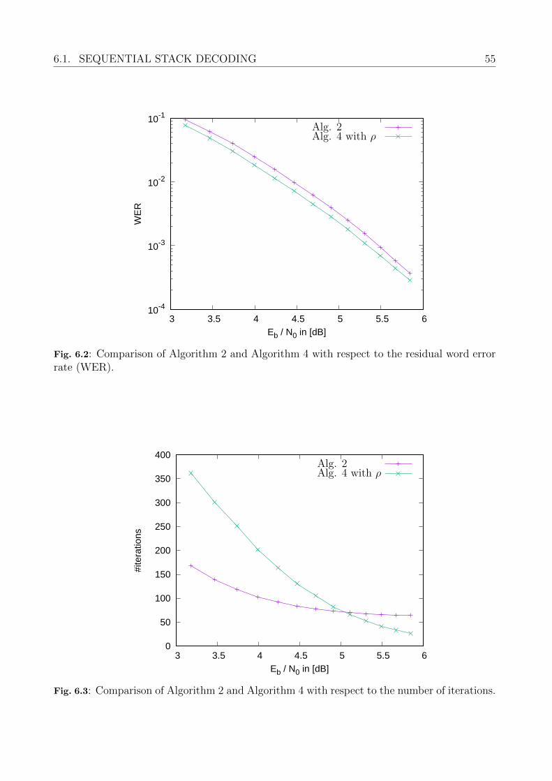
6.1. SEQUENTIAL STACK DECODING 55
10-4
10-3
10-2
10-1
3 3.5 4 4.5 5 5.5 6
WE
R
Eb / N0 in [dB]
Alg. 2Alg. 4 with ρ
Fig. 6.2: Comparison of Algorithm 2 and Algorithm 4 with respect to the residual word errorrate (WER).
0
50
100
150
200
250
300
350
400
3 3.5 4 4.5 5 5.5 6
#ite
ratio
ns
Eb / N0 in [dB]
Alg. 2Alg. 4 with ρ
Fig. 6.3: Comparison of Algorithm 2 and Algorithm 4 with respect to the number of iterations.
56 CHAPTER 6. SOFT-DECODING FOR GENERALIZED CONCATENATED CODES
6.2 GCC Decoding and Decoding Error Probability
In contrast to the decoding procedure presented in Section 4.1.2, the algebraic inner codedecoder is substituted by a soft decoder and thus different column error probabilities Pb,i mustbe considered.
We consider the code level distances da,i of the outer code from Example 3. The lowest levelneeds the highest distance to reach the required WER. While the level increases, the higherobtain the inner code distance db,i. Thus, the outer code error correction capability decreases.Applying soft-decoding in the lower levels starting from i = 0 leads to a higher improvementin decoding complexity and code rate. However, with increasing codeword distance of theinner code in the level i = optimal complexity gets, the complexity increases for the stackalgorithm by O(r2) and its decoding improvements does not lead to a significant complexityreduction in the outer code, which has a complexity of at least O(2n). In this section, we focuson the stack decoding algorithm as inner decoder. The next Section 6.3 discusses alternativesoft-decoding algorithms.
In the first level i = 0 we use soft-input decoding according to Algorithm 2. Starting withthe second level, we exploit the structure of the nested BCH codes and use Algorithm 3, wherethe code at level i−1 can be used as supercode of the code of level i. For the implementation,we limit the number of decoding iterations for each inner code. If the number of iterationsexceeds a threshold a decoding failure is declared. For the outer RS codes we employ error anderasure decoding [69], where the decoding failures of the inner codes are regarded as erasedsymbols of the RS code.
In the following, we present an analysis of the probability of a decoding error for the GCCdecoder. Subsequently, we present an example that illustrates the performance of the proposeddecoding procedure.
6.2.1 Probability of a Decoding Error
The performance of the soft-input decoding of the inner codes can be determined using MonteCarlo simulation. Let Pb,i be the error probability for the decoding of the inner code B(i).Furthermore, let λb,i be the corresponding probability of a decoder failure. We can calculatethe WER using the formulas in Section 4.2.
Example 14. Consider the code from Example 3. This code has a code rate R = 0.806 andwas designed to guarantee WER ≤ 10−16 according to (4.10) for Eb
N0≥ 4.7dB, where soft-input
decoding is used in the first three levels and hard-input decoding in the remaining levels.
6.2.2 Comparison Error Correction Performance
We compare the error correction performance of the GCC in different decoding modes withthe performance of long BCH codes with hard-input decoding. As performance measure, weuse the code rate that is required to guarantee for a given signal to noise ratio an overall worderror rate less than 10−10 or 10−16, respectively. All codes are constructed similar to the codepresented in Example 3. In particular, the inner codes are chosen according to Table 4.1.Whereas the error-correcting capability of the outer codes are adapted to obtain the highestpossible code rate for a given signal to noise ratio. Note that in this example, the overall coderate of the GCC is at most R = 0.9, due to the choice of the inner code.
Figure 6.4 depicts the code rate versus the signal to noise ratio for FER = 10−10, whereasthe results for FER = 10−16 are presented in Figure 6.5. The GCC with soft-input decoding
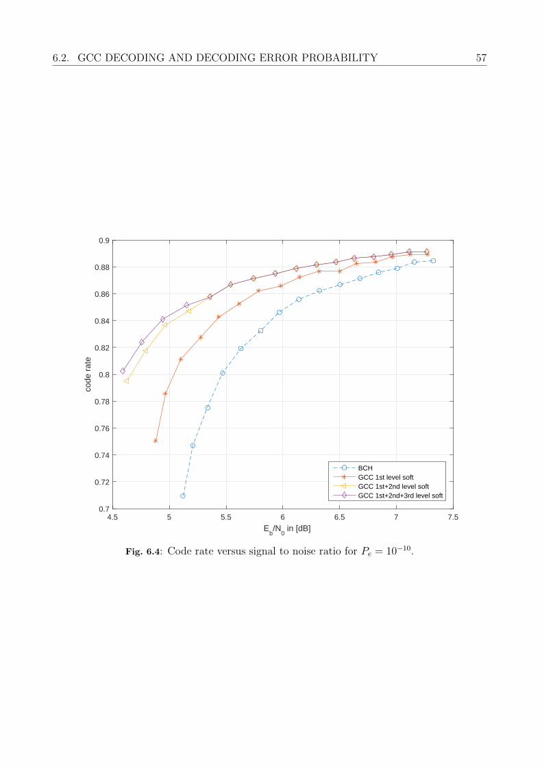
6.2. GCC DECODING AND DECODING ERROR PROBABILITY 57
4.5 5 5.5 6 6.5 7 7.5
Eb/N
0 in [dB]
0.7
0.72
0.74
0.76
0.78
0.8
0.82
0.84
0.86
0.88
0.9
code
rat
e
BCHGCC 1st level softGCC 1st+2nd level softGCC 1st+2nd+3rd level soft
ρ
Fig. 6.4: Code rate versus signal to noise ratio for Pe = 10−10.
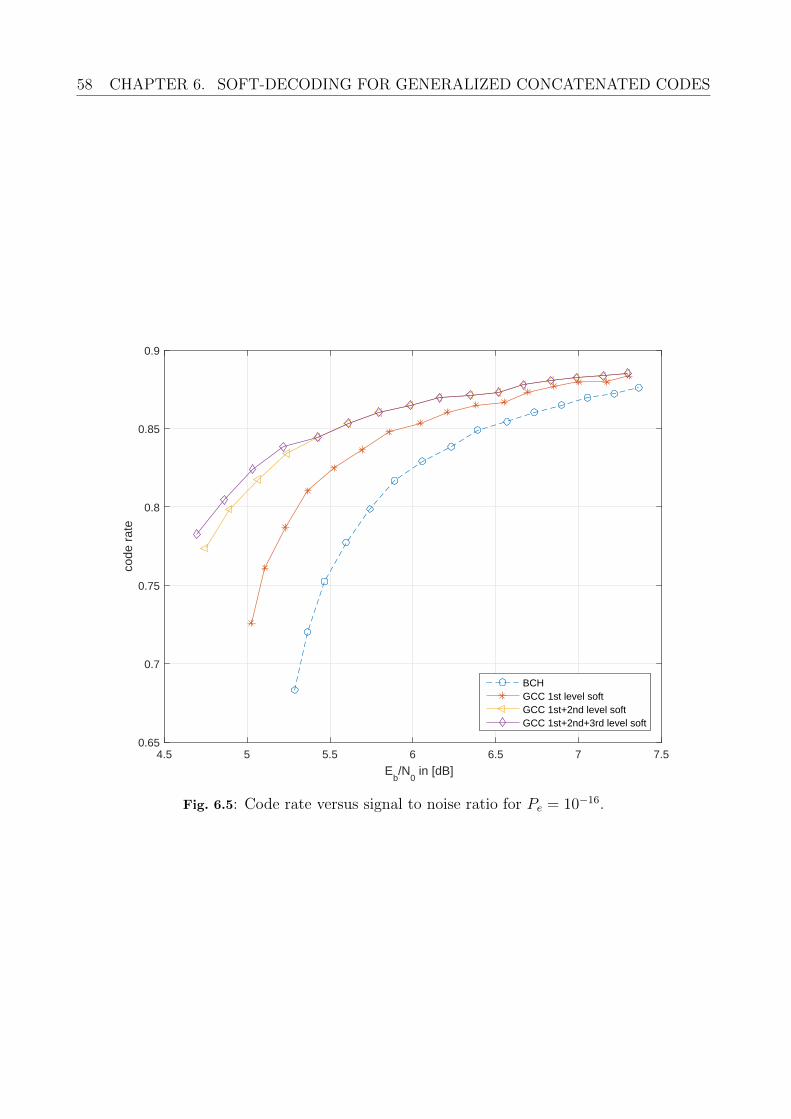
58 CHAPTER 6. SOFT-DECODING FOR GENERALIZED CONCATENATED CODES
4.5 5 5.5 6 6.5 7 7.5
Eb/N
0 in [dB]
0.65
0.7
0.75
0.8
0.85
0.9
code
rat
e
BCHGCC 1st level softGCC 1st+2nd level softGCC 1st+2nd+3rd level soft
ρ
Fig. 6.5: Code rate versus signal to noise ratio for Pe = 10−16.
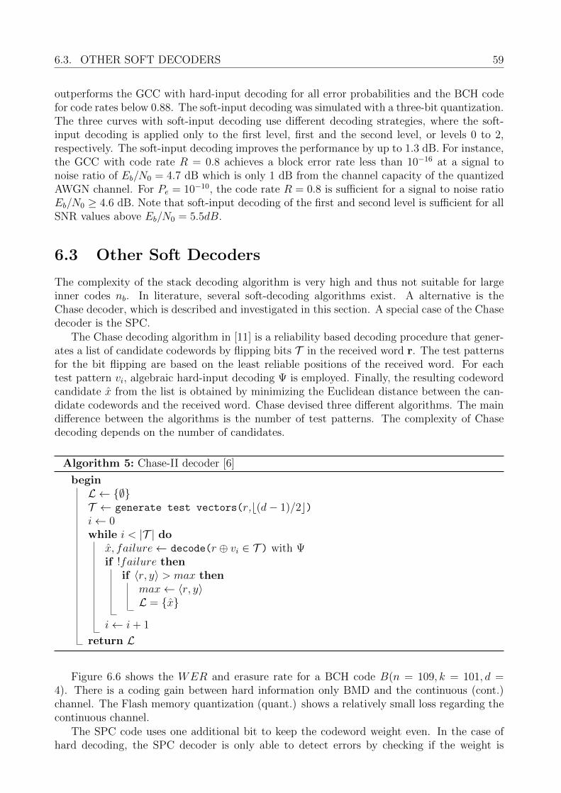
6.3. OTHER SOFT DECODERS 59
outperforms the GCC with hard-input decoding for all error probabilities and the BCH codefor code rates below 0.88. The soft-input decoding was simulated with a three-bit quantization.The three curves with soft-input decoding use different decoding strategies, where the soft-input decoding is applied only to the first level, first and the second level, or levels 0 to 2,respectively. The soft-input decoding improves the performance by up to 1.3 dB. For instance,the GCC with code rate R = 0.8 achieves a block error rate less than 10−16 at a signal tonoise ratio of Eb/N0 = 4.7 dB which is only 1 dB from the channel capacity of the quantizedAWGN channel. For Pe = 10−10, the code rate R = 0.8 is sufficient for a signal to noise ratioEb/N0 ≥ 4.6 dB. Note that soft-input decoding of the first and second level is sufficient for allSNR values above Eb/N0 = 5.5dB.
6.3 Other Soft Decoders
The complexity of the stack decoding algorithm is very high and thus not suitable for largeinner codes nb. In literature, several soft-decoding algorithms exist. A alternative is theChase decoder, which is described and investigated in this section. A special case of the Chasedecoder is the SPC.
The Chase decoding algorithm in [11] is a reliability based decoding procedure that gener-ates a list of candidate codewords by flipping bits T in the received word r. The test patternsfor the bit flipping are based on the least reliable positions of the received word. For eachtest pattern vi, algebraic hard-input decoding Ψ is employed. Finally, the resulting codewordcandidate x from the list is obtained by minimizing the Euclidean distance between the can-didate codewords and the received word. Chase devised three different algorithms. The maindifference between the algorithms is the number of test patterns. The complexity of Chasedecoding depends on the number of candidates.
Algorithm 5: Chase-II decoder [6]
beginL ← ∅T ← generate test vectors(r,b(d− 1)/2c)i← 0while i < |T | do
x, failure← decode(r ⊕ vi ∈ T ) with Ψif !failure then
if 〈r, y〉 > max thenmax← 〈r, y〉L = x
i← i+ 1
return L
Figure 6.6 shows the WER and erasure rate for a BCH code B(n = 109, k = 101, d =4). There is a coding gain between hard information only BMD and the continuous (cont.)channel. The Flash memory quantization (quant.) shows a relatively small loss regarding thecontinuous channel.
The SPC code uses one additional bit to keep the codeword weight even. In the case ofhard decoding, the SPC decoder is only able to detect errors by checking if the weight is
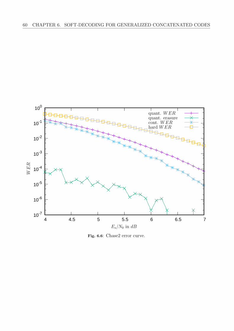
60 CHAPTER 6. SOFT-DECODING FOR GENERALIZED CONCATENATED CODES
10-7
10-6
10-5
10-4
10-3
10-2
10-1
100
4 4.5 5 5.5 6 6.5 7
hard WER
quant. WERquant. erasurecont. WER
WER
Es/N0 in dB
Fig. 6.6: Chase2 error curve.
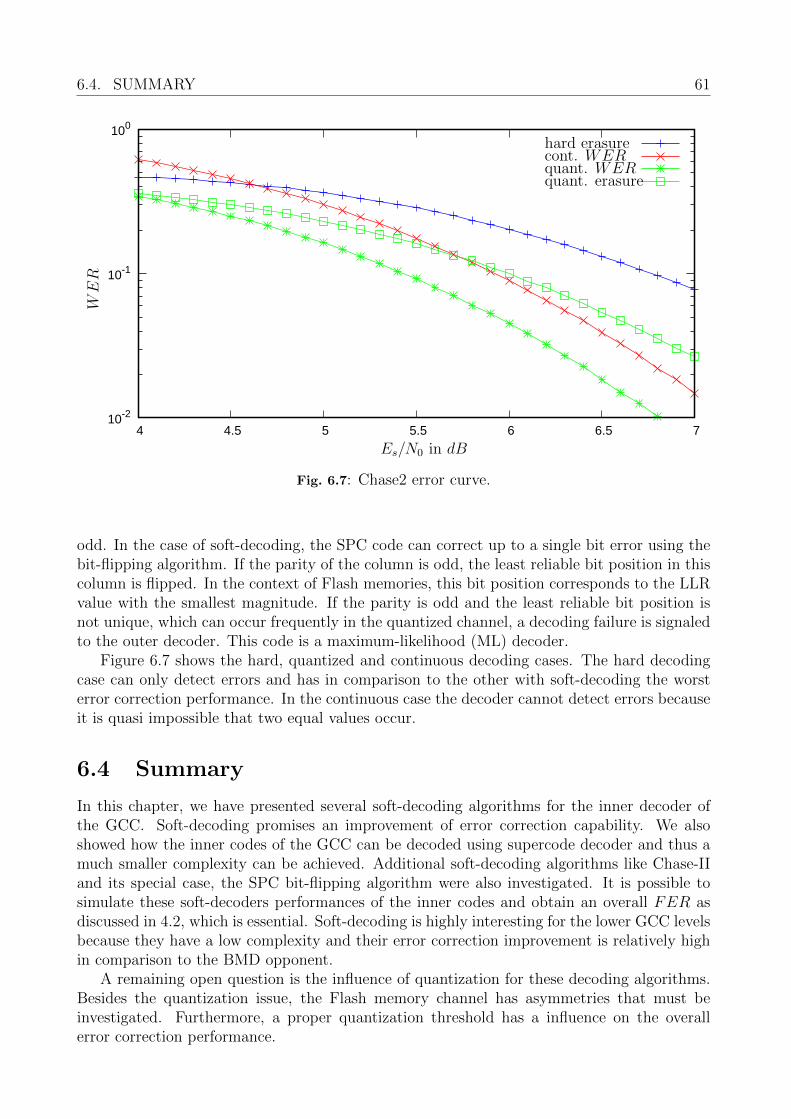
6.4. SUMMARY 61
10-2
10-1
100
4 4.5 5 5.5 6 6.5 7
hard erasure
quant. WERquant. erasure
cont. WER
WER
Es/N0 in dB
Fig. 6.7: Chase2 error curve.
odd. In the case of soft-decoding, the SPC code can correct up to a single bit error using thebit-flipping algorithm. If the parity of the column is odd, the least reliable bit position in thiscolumn is flipped. In the context of Flash memories, this bit position corresponds to the LLRvalue with the smallest magnitude. If the parity is odd and the least reliable bit position isnot unique, which can occur frequently in the quantized channel, a decoding failure is signaledto the outer decoder. This code is a maximum-likelihood (ML) decoder.
Figure 6.7 shows the hard, quantized and continuous decoding cases. The hard decodingcase can only detect errors and has in comparison to the other with soft-decoding the worsterror correction performance. In the continuous case the decoder cannot detect errors becauseit is quasi impossible that two equal values occur.
6.4 Summary
In this chapter, we have presented several soft-decoding algorithms for the inner decoder ofthe GCC. Soft-decoding promises an improvement of error correction capability. We alsoshowed how the inner codes of the GCC can be decoded using supercode decoder and thus amuch smaller complexity can be achieved. Additional soft-decoding algorithms like Chase-IIand its special case, the SPC bit-flipping algorithm were also investigated. It is possible tosimulate these soft-decoders performances of the inner codes and obtain an overall FER asdiscussed in 4.2, which is essential. Soft-decoding is highly interesting for the lower GCC levelsbecause they have a low complexity and their error correction improvement is relatively highin comparison to the BMD opponent.
A remaining open question is the influence of quantization for these decoding algorithms.Besides the quantization issue, the Flash memory channel has asymmetries that must beinvestigated. Furthermore, a proper quantization threshold has a influence on the overallerror correction performance.
62
Chapter 7
Implementation of an Algebraic BCHDecoder
In this chapter, we investigate improvements of the common algebraic BCH decoder im-plementation. This single-block BCH code is the state-of-the-art ECC of nowadays Flashmemory controllers, because it has good performance in correcting independent errors. Anissue of this code is, that the decoder complexity increases at least quadratically with theerror correction capability. There are two significant parameters that lead to this increasedimplementation complexity. First the degree m of the GF (2m) increases to cover theentire data block in comparison to the component codes of the GCC which are shorter.Besides of the degree m the choice of the primitive polynomial has a significant impact onthe implementation complexity. In section 7.2 the impact of the primitive polynomial isinvestigated and an example is given. Second, the error correction capability leads to a higherdegree of the error-location polynomial σ(x), which is determined by the BMA. Severalimplementations are proposed in [57, 72]. Its hardware realization is scalable in throughputor logic. After the BMA has found a solution, the degree of the error-location polynomial isknown. Thus, a multi degree processing Chien search can be constructed that processes thepolynomial with different speeds and with that a trade-off between throughput versus diearea can be realized. An approach to a mixed solution is presented in 7.1.
The novelties in this chapter are:
• A mixed parallel and serial BCH implementation design and its analysis. (Publishedin [82, 95])
• Investigations on Galois field optimizations and its application in mixed GF BCH decoderimplementations.
7.1 A Mixed Parallel and Serial BCH Implementation
In this section, we provide an overview of a BCH implementation. It exists several modulesthat can be scaled differently. Because the decoding complexity grows quadratically with theerror correction capability t, modifications in the state-of-the-art BMA and Chien search arediscussed to trade-off between speed and die area.
Algebraic decoding of BCH codes consists of the following four steps, which are usuallyrealized in modules in a hardware implementation:
7.1. A MIXED PARALLEL AND SERIAL BCH IMPLEMENTATION 63
1. Calculating the Syndrome
2. Calculation of the error-location polynomial (BMA)
3. Evaluation of the error-location polynomial (Chien search)
4. Correcting the erroneous positions
Steps 2 and 3 dominate the computational complexity and therefore the area that is re-quired for a hardware implementation. Both decoding steps can be realized with serial andparallel implementations. A parallel implementation achieves larger throughput but also re-quires more area than a serial implementation.
7.1.1 Syndrome Computation
In practice the codeword is read word-wise, i.e. 8 or 16 bit per cycle. The decoder calculatesthe syndrome values in parallel for each syndrome Si using Horner’s rule, which calculates ncodeword bits per iteration. Using Horner’s rule means processing with the most significantbit or degree first.
In common the calculation of the syndrome S can be expressed as a matrix multiplicationof the check matrix H and the received codeword r, by
S = Hr . (7.1)
In order to scale the syndrome calculation between logic complexity and throughput, thepartial syndrome vector S ′ is determined by a reduced k′ × i checkmatrix.
S′ =
α0 α1 . . . αk
′−1
α0 α2 . . . α2(k′−1)
......
. . ....
α0 αi . . . αi(k′−1)
· r0
...rk′−1
(7.2)
S′ represents the fraction of the Horner’s rule. This is then added to a feedback register, whichis then multiplied by αik
′where i is the index of the syndrome value and k′ is the size of the
portion of the entire codeword.In polynomial form it can be expressed as
Si(αi) = (. . . (rn−0α
0 + . . .+ rn−k′−1αi(k′−1))αik
′+ (7.3)
rn−k′ . . . rn−2k′−1αi(k′−1))αik
′+
rn−2k′ . . . rn−3k′−1αi(k′−1) + . . .)αik
′+
r′kα0 + . . . r0α
i(k′−1)
where the characteristic of the Horner scheme can be recognized.Due to the symmetry of the binary BCH code the even indexed syndrome values are linear
dependent on the odd indexed syndrome values. This property can be used to reduce theimplementation complexity. All even indexed syndrome values can be calculated by the squareor multiple square of an odd indexed syndrome value, when all odd indexed syndrome valuesare ready. This technique reduces the number of registers to store the intermediate syndromevalues but leads to a higher latency in the case of multiple squaring, which affects only the lastcycle and thus can be solved by a multi-cycle path. Alternatively, the even syndrome valuesS2i can be calculated in the i-th iteration of the BMA with a single multiplier but additionalmultiplexers and thus area and timing are reduced.
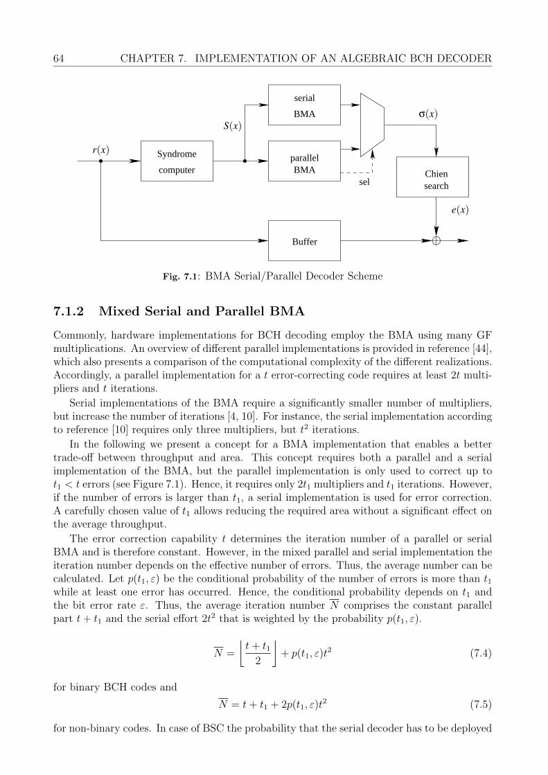
64 CHAPTER 7. IMPLEMENTATION OF AN ALGEBRAIC BCH DECODER
Buffer
Syndrome
computer BMAparallel
serial
BMA
sel searchChien
S(x)
r(x)
e(x)
σ(x)
dB
Fig. 7.1: BMA Serial/Parallel Decoder Scheme
7.1.2 Mixed Serial and Parallel BMA
Commonly, hardware implementations for BCH decoding employ the BMA using many GFmultiplications. An overview of different parallel implementations is provided in reference [44],which also presents a comparison of the computational complexity of the different realizations.Accordingly, a parallel implementation for a t error-correcting code requires at least 2t multi-pliers and t iterations.
Serial implementations of the BMA require a significantly smaller number of multipliers,but increase the number of iterations [4, 10]. For instance, the serial implementation accordingto reference [10] requires only three multipliers, but t2 iterations.
In the following we present a concept for a BMA implementation that enables a bettertrade-off between throughput and area. This concept requires both a parallel and a serialimplementation of the BMA, but the parallel implementation is only used to correct up tot1 < t errors (see Figure 7.1). Hence, it requires only 2t1 multipliers and t1 iterations. However,if the number of errors is larger than t1, a serial implementation is used for error correction.A carefully chosen value of t1 allows reducing the required area without a significant effect onthe average throughput.
The error correction capability t determines the iteration number of a parallel or serialBMA and is therefore constant. However, in the mixed parallel and serial implementation theiteration number depends on the effective number of errors. Thus, the average number can becalculated. Let p(t1, ε) be the conditional probability of the number of errors is more than t1while at least one error has occurred. Hence, the conditional probability depends on t1 andthe bit error rate ε. Thus, the average iteration number N comprises the constant parallelpart t+ t1 and the serial effort 2t2 that is weighted by the probability p(t1, ε).
N =
⌊t+ t1
2
⌋+ p(t1, ε)t
2 (7.4)
for binary BCH codes and
N = t+ t1 + 2p(t1, ε)t2 (7.5)
for non-binary codes. In case of BSC the probability that the serial decoder has to be deployed
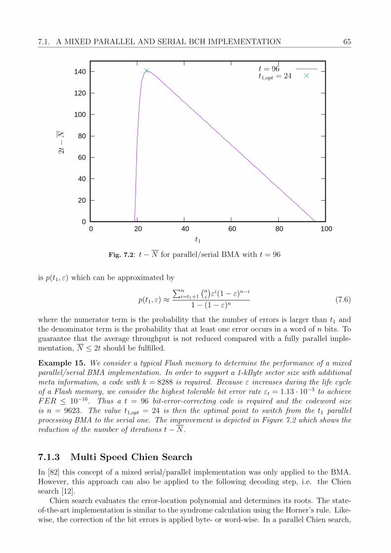
7.1. A MIXED PARALLEL AND SERIAL BCH IMPLEMENTATION 65
0
20
40
60
80
100
120
140
0 20 40 60 80 100
2t−
N
t1
t = 96t1,opt = 24
Fig. 7.2: t−N for parallel/serial BMA with t = 96
is p(t1, ε) which can be approximated by
p(t1, ε) ≈∑n
i=t1+1
(ni
)εi(1− ε)n−i
1− (1− ε)n(7.6)
where the numerator term is the probability that the number of errors is larger than t1 andthe denominator term is the probability that at least one error occurs in a word of n bits. Toguarantee that the average throughput is not reduced compared with a fully parallel imple-mentation, N ≤ 2t should be fulfilled.
Example 15. We consider a typical Flash memory to determine the performance of a mixedparallel/serial BMA implementation. In order to support a 1-kByte sector size with additionalmeta information, a code with k = 8288 is required. Because ε increases during the life cycleof a Flash memory, we consider the highest tolerable bit error rate εt = 1.13 · 10−3 to achieveFER ≤ 10−16. Thus a t = 96 bit-error-correcting code is required and the codeword sizeis n = 9623. The value t1,opt = 24 is then the optimal point to switch from the t1 parallelprocessing BMA to the serial one. The improvement is depicted in Figure 7.2 which shows thereduction of the number of iterations t−N .
7.1.3 Multi Speed Chien Search
In [82] this concept of a mixed serial/parallel implementation was only applied to the BMA.However, this approach can also be applied to the following decoding step, i.e. the Chiensearch [12].
Chien search evaluates the error-location polynomial and determines its roots. The state-of-the-art implementation is similar to the syndrome calculation using the Horner’s rule. Like-wise, the correction of the bit errors is applied byte- or word-wise. In a parallel Chien search,
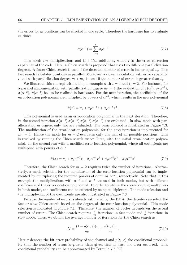
66 CHAPTER 7. IMPLEMENTATION OF AN ALGEBRAIC BCH DECODER
the errors for m positions can be checked in one cycle. Therefore the hardware has to evaluatem times
σ(α−l) =t∑i=0
σiα−li (7.7)
This needs tm multiplications and (t + 1)m additions, where t is the error correctioncapability of the code. Here, a Chien search is proposed that uses two different parallelizationdegrees. A faster Chien search is used if the detected number of errors is less or equal t1. Thisfast search calculates positions in parallel. Moreover, a slower calculation with error capabilityt and with parallelization degree m < m1 is used if the number of errors is greater than t1.
We illustrate this concept with a simple example with t = 4 and t1 = 2. For instance, fora parallel implementation with parallelization degree m1 = 4 the evaluation of σ(α0), σ(α−1),σ(α−2), σ(α−3) has to be realized in hardware. For the next iteration, the coefficients of theerror-location polynomial are multiplied by powers of α−4, which results in the new polynomial
σ(x) = σ0 + σ1α−4x+ σ2α
−8x2 . (7.8)
This polynomial is used as an error-location polynomial in the next iteration. Therefore,in the second iteration σ(α−4),σ(α−5),σ(α−6),σ(α−7) are evaluated. In slow mode with par-allelization m degree, only two are evaluated. The basic concept is illustrated in Figure 7.3.The modification of the error-location polynomial for the next iteration is implemented form1 = 4. Hence the mode for m = 2 evaluates only one half of all possible positions. Thisis resolved by running the Chien search twice: First, with the initial error-location polyno-mial. In the second run with a modified error-location polynomial, where all coefficients aremultiplied with powers of α−2
σ(x) = σ0 + σ1α−2x+ σ2α
−4x2 + σ3α−6x3 + σ4α
−8x4 (7.9)
Therefore, the Chien search for m = 2 requires twice the number of iterations. Alterna-tively, a mode selection for the modification of the error-location polynomial can be imple-mented by multiplexing the required powers of α−m1 or α−m, respectively. Note that in thisexample the multiplications with α−3 and α−4 are used in both modes, but with differentcoefficients of the error-location polynomial. In order to utilize the corresponding multipliersin both modes, the coefficients can be selected by using multiplexers. The mode selection andthe multiplexing of the coefficients are also illustrated in Figure 7.3.
Because the number of errors is already estimated by the BMA, the decoder can select thefast or slow Chien search based on the degree of the error-location polynomial. This modeselection is indicated in Figure 7.1. Therefore, the number of cycles depends on the actualnumber of errors. The Chien search requires n
m1iterations in fast mode and n
miterations in
slow mode. Thus, we obtain the average number of iterations for the Chien search as
N =(1− p(t1, ε))n
m1
+p(t1, ε)n
m. (7.10)
Here ε denotes the bit error probability of the channel and p(t1, ε) the conditional probabil-ity that the number of errors is greater than given that at least one error occurred. Thisconditional probability can be approximated by Formula 7.6 [82].
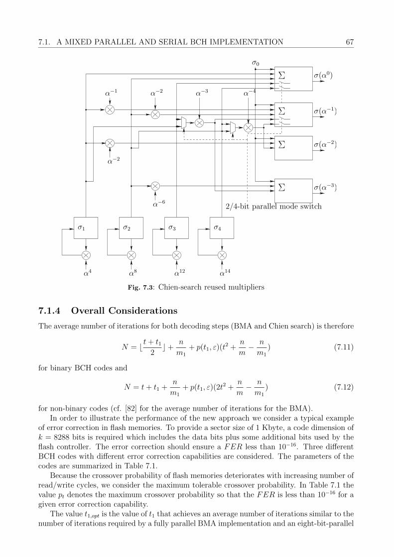
7.1. A MIXED PARALLEL AND SERIAL BCH IMPLEMENTATION 67
Σ
Σ
Σ
Σ
σ0
σ1 σ2 σ3 σ4
α4 α8 α12 α14
σ(α0)
σ(α−1)
σ(α−2)
σ(α−3)
α−1 α−2
α−2
α−3 α−4
α−62/4-bit parallel mode switch
Fig. 7.3: Chien-search reused multipliers
7.1.4 Overall Considerations
The average number of iterations for both decoding steps (BMA and Chien search) is therefore
N = bt+ t12c+
n
m1
+ p(t1, ε)(t2 +
n
m− n
m1
) (7.11)
for binary BCH codes and
N = t+ t1 +n
m1
+ p(t1, ε)(2t2 +
n
m− n
m1
) (7.12)
for non-binary codes (cf. [82] for the average number of iterations for the BMA).In order to illustrate the performance of the new approach we consider a typical example
of error correction in flash memories. To provide a sector size of 1 Kbyte, a code dimension ofk = 8288 bits is required which includes the data bits plus some additional bits used by theflash controller. The error correction should ensure a FER less than 10−16. Three differentBCH codes with different error correction capabilities are considered. The parameters of thecodes are summarized in Table 7.1.
Because the crossover probability of flash memories deteriorates with increasing number ofread/write cycles, we consider the maximum tolerable crossover probability. In Table 7.1 thevalue pt denotes the maximum crossover probability so that the FER is less than 10−16 for agiven error correction capability.
The value t1,opt is the value of t1 that achieves an average number of iterations similar to thenumber of iterations required by a fully parallel BMA implementation and an eight-bit-parallel
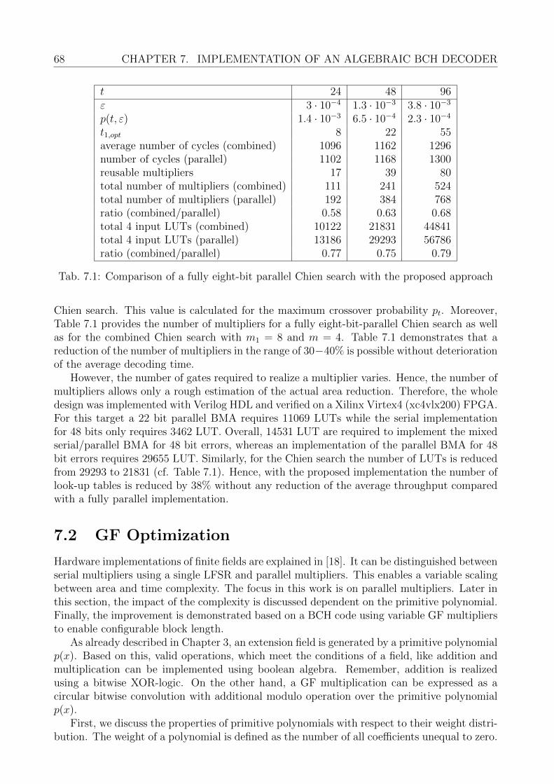
68 CHAPTER 7. IMPLEMENTATION OF AN ALGEBRAIC BCH DECODER
t 24 48 96ε 3 · 10−4 1.3 · 10−3 3.8 · 10−3
p(t, ε) 1.4 · 10−3 6.5 · 10−4 2.3 · 10−4
t1,opt 8 22 55average number of cycles (combined) 1096 1162 1296number of cycles (parallel) 1102 1168 1300reusable multipliers 17 39 80total number of multipliers (combined) 111 241 524total number of multipliers (parallel) 192 384 768ratio (combined/parallel) 0.58 0.63 0.68total 4 input LUTs (combined) 10122 21831 44841total 4 input LUTs (parallel) 13186 29293 56786ratio (combined/parallel) 0.77 0.75 0.79
Tab. 7.1: Comparison of a fully eight-bit parallel Chien search with the proposed approach
Chien search. This value is calculated for the maximum crossover probability pt. Moreover,Table 7.1 provides the number of multipliers for a fully eight-bit-parallel Chien search as wellas for the combined Chien search with m1 = 8 and m = 4. Table 7.1 demonstrates that areduction of the number of multipliers in the range of 30−40% is possible without deteriorationof the average decoding time.
However, the number of gates required to realize a multiplier varies. Hence, the number ofmultipliers allows only a rough estimation of the actual area reduction. Therefore, the wholedesign was implemented with Verilog HDL and verified on a Xilinx Virtex4 (xc4vlx200) FPGA.For this target a 22 bit parallel BMA requires 11069 LUTs while the serial implementationfor 48 bits only requires 3462 LUT. Overall, 14531 LUT are required to implement the mixedserial/parallel BMA for 48 bit errors, whereas an implementation of the parallel BMA for 48bit errors requires 29655 LUT. Similarly, for the Chien search the number of LUTs is reducedfrom 29293 to 21831 (cf. Table 7.1). Hence, with the proposed implementation the number oflook-up tables is reduced by 38% without any reduction of the average throughput comparedwith a fully parallel implementation.
7.2 GF Optimization
Hardware implementations of finite fields are explained in [18]. It can be distinguished betweenserial multipliers using a single LFSR and parallel multipliers. This enables a variable scalingbetween area and time complexity. The focus in this work is on parallel multipliers. Later inthis section, the impact of the complexity is discussed dependent on the primitive polynomial.Finally, the improvement is demonstrated based on a BCH code using variable GF multipliersto enable configurable block length.
As already described in Chapter 3, an extension field is generated by a primitive polynomialp(x). Based on this, valid operations, which meet the conditions of a field, like addition andmultiplication can be implemented using boolean algebra. Remember, addition is realizedusing a bitwise XOR-logic. On the other hand, a GF multiplication can be expressed as acircular bitwise convolution with additional modulo operation over the primitive polynomialp(x).
First, we discuss the properties of primitive polynomials with respect to their weight distri-bution. The weight of a polynomial is defined as the number of all coefficients unequal to zero.
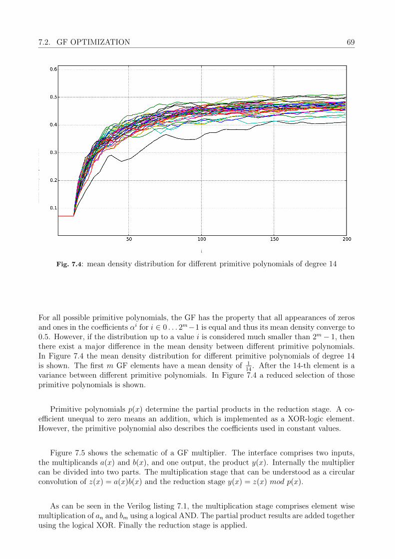
7.2. GF OPTIMIZATION 69meandensity
ofpow
ersof
α
i
Fig. 7.4: mean density distribution for different primitive polynomials of degree 14
For all possible primitive polynomials, the GF has the property that all appearances of zerosand ones in the coefficients αi for i ∈ 0 . . . 2m−1 is equal and thus its mean density converge to0.5. However, if the distribution up to a value i is considered much smaller than 2m− 1, thenthere exist a major difference in the mean density between different primitive polynomials.In Figure 7.4 the mean density distribution for different primitive polynomials of degree 14is shown. The first m GF elements have a mean density of 1
14. After the 14-th element is a
variance between different primitive polynomials. In Figure 7.4 a reduced selection of thoseprimitive polynomials is shown.
Primitive polynomials p(x) determine the partial products in the reduction stage. A co-efficient unequal to zero means an addition, which is implemented as a XOR-logic element.However, the primitive polynomial also describes the coefficients used in constant values.
Figure 7.5 shows the schematic of a GF multiplier. The interface comprises two inputs,the multiplicands a(x) and b(x), and one output, the product y(x). Internally the multipliercan be divided into two parts. The multiplication stage that can be understood as a circularconvolution of z(x) = a(x)b(x) and the reduction stage y(x) = z(x) mod p(x).
As can be seen in the Verilog listing 7.1, the multiplication stage comprises element wisemultiplication of an and bm using a logical AND. The partial product results are added togetherusing the logical XOR. Finally the reduction stage is applied.
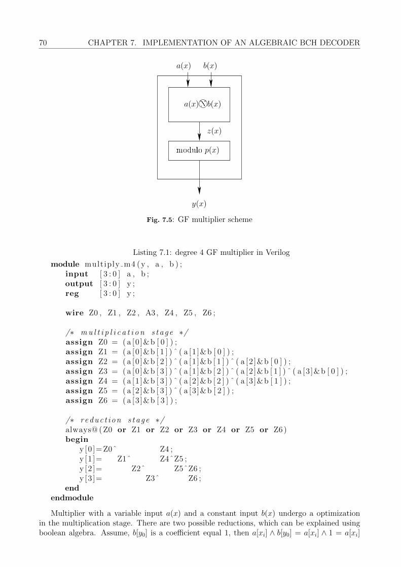
70 CHAPTER 7. IMPLEMENTATION OF AN ALGEBRAIC BCH DECODER
a(x) b(x)
z(x)
y(x)
modulo p(x)
a(x)N b(x)
i
Fig. 7.5: GF multiplier scheme
Listing 7.1: degree 4 GF multiplier in Verilog
module multiply m4 (y , a , b ) ;input [ 3 : 0 ] a , b ;output [ 3 : 0 ] y ;reg [ 3 : 0 ] y ;
wire Z0 , Z1 , Z2 , A3 , Z4 , Z5 , Z6 ;
/∗ m u l t i p l i c a t i o n s t a g e ∗/assign Z0 = ( a [0 ]&b [ 0 ] ) ;assign Z1 = ( a [0 ]&b [ 1 ] ) ˆ ( a [1 ]&b [ 0 ] ) ;assign Z2 = ( a [0 ]&b [ 2 ] ) ˆ ( a [1 ]&b [ 1 ] ) ˆ ( a [2 ]&b [ 0 ] ) ;assign Z3 = ( a [0 ]&b [ 3 ] ) ˆ ( a [1 ]&b [ 2 ] ) ˆ ( a [2 ]&b [ 1 ] ) ˆ ( a [3 ]&b [ 0 ] ) ;assign Z4 = ( a [1 ]&b [ 3 ] ) ˆ ( a [2 ]&b [ 2 ] ) ˆ ( a [3 ]&b [ 1 ] ) ;assign Z5 = ( a [2 ]&b [ 3 ] ) ˆ ( a [3 ]&b [ 2 ] ) ;assign Z6 = ( a [3 ]&b [ 3 ] ) ;
/∗ r e d u c t i o n s t a g e ∗/always@ (Z0 or Z1 or Z2 or Z3 or Z4 or Z5 or Z6)begin
y [0 ]= Z0ˆ Z4 ;y [1 ]= Z1ˆ Z4ˆZ5 ;y [2 ]= Z2ˆ Z5ˆZ6 ;y [3 ]= Z3ˆ Z6 ;
endendmodule
Multiplier with a variable input a(x) and a constant input b(x) undergo a optimizationin the multiplication stage. There are two possible reductions, which can be explained usingboolean algebra. Assume, b[y0] is a coefficient equal 1, then a[xi] ∧ b[y0] = a[xi] ∧ 1 = a[xi]
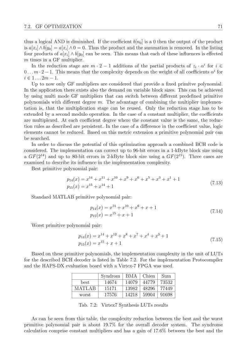
7.2. GF OPTIMIZATION 71
thus a logical AND is diminished. If the coefficient b[n0] is a 0 then the output of the productis a[xi]∧ b[y0] = a[xi]∧ 0 = 0. Thus the product and the summation is removed. In the listingfour products of a[xi] ∧ b[y0] can be seen. This means that each of these influences is effectedm times in a GF multiplier.
In the reduction stage are m · 2 − 1 additions of the partial products of zi · αi for i ∈0 . . .m · 2− 1. This means that the complexity depends on the weight of all coefficients αi fori ∈ 1 . . . 2m− 1.
Up to now only GF multipliers are considered that provide a fixed primitve polynomial.In the application there exists also the demand on variable block sizes. This can be achievedby using multi mode GF multipliers that can switch between different predefined primitivepolynomials with different degree m. The advantage of combining the multiplier implemen-tation is, that the multiplication stage can be reused. Only the reduction stage has to beextended by a second modulo operation. In the case of a constant multiplier, the coefficientsare multiplexed. At each coefficient degree where the constant value is the same, the reduc-tion rules as described are persistent. In the case of a difference in the coefficient value, logicelements cannot be reduced. Based on this metric extension a primitive polynomial pair canbe searched.
In order to discuss the potential of this optimization approach a combined BCH code isconsidered. The implementation can correct up to 96-bit errors in a 1-kByte block size usinga GF (214) and up to 80-bit errors in 2-kByte block size using a GF (215). Three cases areexamined to describe its influence in the implementation complexity.
Best primitive polynomial pair:
p14(x) = x14 + x11 + x10 + x9 + x6 + x5 + x3 + x1 + 1
p15(x) = x15 + x14 + 1(7.13)
Standard MATLAB primitive polynomial pair:
p14(x) = x14 + x10 + x6 + x+ 1
p15(x) = x15 + x+ 1(7.14)
Worst primitive polynomial pair:
p14(x) = x14 + x12 + x8 + x7 + x4 + x3 + 1
p15(x) = x15 + x+ 1(7.15)
Based on these primitive polynomials, the implementation complexity in the unit of LUTsfor the described BCH decoder is listed in Table 7.2. For the implementation Protocompilerand the HAPS-DX evaluation board with a Virtex-7 FPGA was used.
Syndrom BMA Chien Sumbest 14674 14079 44779 73532
MATLAB 15171 13982 48296 77449worst 17576 14218 59904 91698
Tab. 7.2: Virtex7 Synthesis LUTs results
As can be seen from this table, the complexity reduction between the best and the worstprimitive polynomial pair is about 19.7% for the overall decoder system. The syndromecalculation comprise constant multipliers and has a gain of 17.6% between the best and the
72 CHAPTER 7. IMPLEMENTATION OF AN ALGEBRAIC BCH DECODER
worst primitive polynomial pair. A lower gain can be seen in the BMA because it consistsonly of full multipliers where takes only an effect in the modulo stage. It can be seen fromTable 7.2 that the Chien search has the largest number of constant multipliers, with a gain of26.5%.
7.3 Summary
This chapter described the improvements for a state-of-the-art flash controller BCH decoder.In Section 7.1 a combination of a mixed parallel and serial BMA and a multi speed Chiensearch was discussed. Its goal was to handle a trade-off between implementation size andthroughput that depends on the RBER. It was shown how an optimal ratio between paralleland serial calculation is determined. We have also shown the area reduction of 38% for anexemplar 48 error-correcting BCH FPGA implementation.
In Section 7.2 the optimization of the GF arithmetic was discussed. The primitive poly-nomial has an impact on the necessary logic in constant and full multipliers. By means of anexample, it was shown that an FPGA synthesis area results between the best and worst casescenario makes a difference of 19.7%.
These optimizations are applicable in the GCC. The BMA of the inner GCC code isa candidate of a mixed parallel and serial implementation. At least one error is occurringrelatively often. The highest level of the nested BCH code then determines the t1 of theparallel BMA. E.g. tb,L−1 = 13 then t1 = 7 is able to correct all single errors in the laterdescribed pipelined BMA. If more errors occur in a column, then the pipeline is stoppedand the remaining degrees of the error-location polynomial are calculated in a serial BMAimplementation.
Because the component codes rely on the GF arithmetic, the GF optimization also affectsthe size of the overall GCC implementation.

73
Chapter 8
Implementation of GCC withHardinformation
In this chapter, the focus is placed on the hardware implementation of the proposed pipelinedGCC decoder from Chapter 4. Chapter 7 was a starting point for the implementation of thecomponent BCH codes and in parts of the RS codes. The main difference for the GCC innerBCH codes are the error correction capability, the bit width of the syndrome, Chien search,and the pipelined BMA. Moreover, the outer RS codes need a key equation solver thatconsiders erasures and calculates an additional error-value polynomial. We also describe theGCC encoder whose BCH encoder model is similarly used in the re-imageing and re-encodingstep of the decoder. In Section 8.1 we describe a realization of the decoding scheme fromFigure 8.1 in hardware. Beside the question of the logic complexity, the requirements forbuffers are investigated in Section 8.2. In Section 8.3 a comparison between a state-of-the-artBCH code and the GCC is presented. Finally, in Section 8.4 an outlook of improvements thatrequire further investigations is provided.
The novelties in this chapter are:
• A GCC hardware design for hard information decoding and
• its analysis regarding throughput and area consumption.
Parts of this chapter are published in [88, 91, 92, 99].
8.1 GCC Data Matrix and Pipelined Decoder
In this section, we draw a hardware design of the GCC decoder that is refined step-by-step.Figure 8.1 shows the decoding scheme which serves as implementation guideline. In this figurerepeating tasks for the levels can be identified which differ in the code distance parameter.Thus, a received codeword is processed several times by the same decoder modules that areconfigurable. From this starting point we develop a decoder architecture. In order to achievea high throughput, a pipelined approach is developed.
Due to the small GF alphabet and the small error correction capability of the BCH codes,the implementation allows an efficient pipelining structure as proposed in Figure 8.1. Ex-cept the BMA algorithm for the outer RS codes all decoding components are arranged in apipelining structure. We explain Figure 8.1 from left to the right.
In order to store the received word the decoder has a data matrix buffer which is imple-mented as a shift register. This shift register has na + DBCH columns where each column is
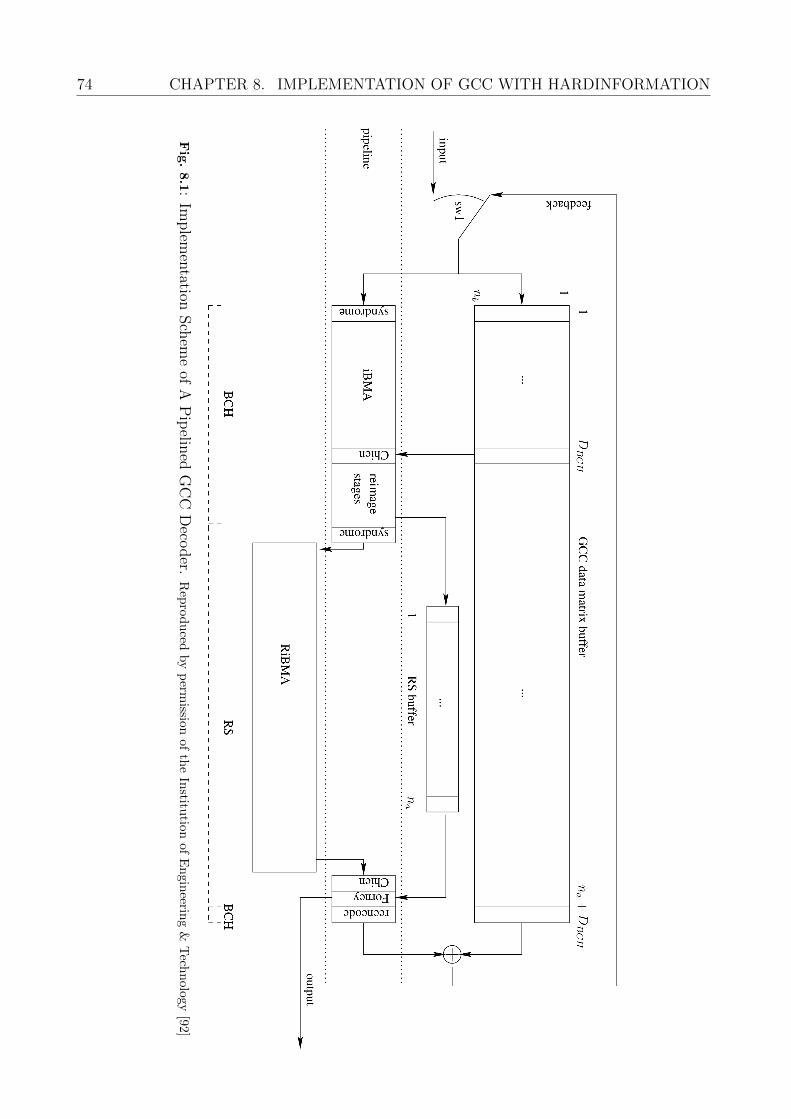
74 CHAPTER 8. IMPLEMENTATION OF GCC WITH HARDINFORMATION
Fig.8.1:
Implem
entation
Sch
eme
ofA
Pip
elined
GC
CD
ecoder.
Rep
rod
uced
by
perm
issionof
the
Institu
tionof
En
gineerin
g&
Tech
nology
[92]
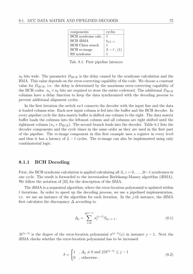
8.1. GCC DATA MATRIX AND PIPELINED DECODER 75
components cycles
BCH syndrome calc. 1BCH iBMA tb,L−1
BCH Chien search 1BCH re-image L− l , (1)RS syndrome 1
Tab. 8.1: First pipeline latencys
nb bits wide. The parameter DBCH is the delay caused by the syndrome calculation and theBMA. This value depends on the error-correcting capability of the code. We choose a constantvalue for DBCH , i.e. the delay is determined by the maximum error-correcting capability ofthe BCH codes. na × nb bits are required to store the entire codeword. The additional DBCH
columns have a delay function to keep the data synchronized with the decoding process toprevent additional alignment cycles.
In the first iteration the switch sw1 connects the decoder with the input line and the datais loaded column-wise. Each new input column is fed into the buffer and the BCH decoder. Inevery pipeline cycle the data matrix buffer is shifted one column to the right. The data matrixbuffer loads the columns into the leftmost column and all columns are right shifted until therightmost column (na +DBCH). The second branch leads into the decoder. Table 8.1 lists thedecoder components and the cycle times in the same order as they are used in the first partof the pipeline. The re-image component in this first example uses a register in every leveland thus it has a latency of L − l cycles. The re-image can also be implemented using onlycombinatorial logic.
8.1.1 BCH Decoding
First, the BCH syndrome calculation is applied calculating all Si, i = 0, . . . , 2t−1 syndromes inone cycle. The result is forwarded to the inversionless Berlekamp-Massey algorithm (iBMA).We follow the notation of [35] for the description of the BMA.
The iBMA is a sequential algorithm, where the error-location polynomial is updated withint iterations. In order to speed up the decoding process, we use a pipelined implementation,i.e. we use an instance of the algorithm for each iteration. In the j-th instance, the iBMAfirst calculates the discrepancy ∆ according to
∆j =M(j−1)∑i=0
σ(j−1)i S2j−i−1 . (8.1)
M (j−1) is the degree of the error-location polynomial σ(j−1)(x) in instance j − 1. Next theiBMA checks whether the error-location polynomial has to be increased
δ =
1 , ∆j 6= 0 and 2M (j−1) ≤ j − 1
0 , otherwise .(8.2)
76 CHAPTER 8. IMPLEMENTATION OF GCC WITH HARDINFORMATION
Finally, the iBMA updates σ(j−1)(x) according to
[σ(j)(x)ν(j)(x)
]=
[θ(j−1) −∆jxδ (1− δ)x
]·[σ(j−1)(x)ν(j−1)(x)
]θ(j) = δ∆j + (1− δ)θ(j−1) and
M (j) = δ(k −M (j−1)) + (1− δ)M (j−1) .
(8.3)
Here, ν(j)(x) is a supporting polynomial that is required for the update of the error-locationpolynomial. The variable θ(j) controls the multiplication to avoid inversions.
From these equations follows that the number of multiplications for the discrepancy andthe update of σ(x) and ν(x) are growing with the degree M (j) of σ(x). Hence, the first stagesrequire fewer finite field multipliers. Moreover, the iBMA has to be configurable to solve thekey equation for all possible error-correcting capabilities of the inner codes.
In the next pipeline step, the Chien search checks all roots for each error position in parallel.The evaluation of the error-location polynomial is implemented to solve all multiplications andadditions in one cycle. In the same cycle the column codeword is corrected by loading thecolumn DBCH and flipping the bits at the detected error positions. The corrected columncodeword is then fed into the BCH re-imaging stages.
The iBMA using the update rule in Eq. (8.3) does not change for even syndrome valuedue to their linear dependencies. Thus the update rule can be modified such that it takes theeven 2i and odd 2i+ 1 syndrome values into account
[σ(j)(x)ν(j)(x)
]=
[(1− δ)θ2(j−1) + δ∆jθ
(j−1) −δ∆2jν
(j−1)(x)δx (1− δ)x2
] [σ(j−1)(x)ν(j−1)(x)
]θ(j) = (1− δ)θ(j−1) + δ∆jθ
(j−1)
L(j) = (1− δ)L(j−1) + δ(k − L(j−1)) .
(8.4)
Using Eq. (8.4), the intermediate steps need no registers and thus this solution is smaller andneeds half the number of cycles as Eq. (8.3)
8.1.2 Re-imaging
The re-imaging process is the inverse mapping of the encoding of a column codeword whichis depicted in Figure 4.6. Each re-image stage comprises a direct encoder implementation forthe corresponding inner code. Hence, the re-imaging stage is equivalent to the encoding of theinner codes in the GCC encoder. In each clock cycle the codeword is inferred for one level untilthe desired level is reached. Figure 8.2 shows how the pipelined encoders are implemented ina cascaded form, where the information aj,i of level i is first encoded and then the parity pj,iis subtracted from the column codeword.
After a latency of L− l cycles, which is caused by the re-imaging process, the current RScodeword row i is selected by a de-multiplexer. Subsequently, the RS symbol aj,i is stored inthe RS buffer, which stores an entire outer codeword ai. The symbol aj,i is loaded into thenext cycle of the RS syndrome calculator.
8.1. GCC DATA MATRIX AND PIPELINED DECODER 77
input output
pj,2 pj−1,1
B(2)
aj−1,1
aj−1,2
aj−2,0
B(1) aj−2,1
aj−2,2aj,2i
Fig. 8.2: BCH re-image cascade. Reproduced by permission of the Institution of Engineering & Tech-nology [92]
8.1.3 RS decoding
The syndrome for the RS code is calculated using Horner’s rule
Si(αi) = (. . . (rnα
i + rn−1)αi + rn−2) + . . .)αi + r0 . (8.5)
This has three advantages:
• The RS codeword is arriving symbol-wise and the syndroms can be calculated symbol-wise.
• The RS codeword is read in reverse order which simplifies the Chien search and theForney algorithm.
• Horner’s method only needs a single multiplier and a single adder per syndrome value.
• The Horner’s method can also be partially parallelized such that n symbols can becalculated at once (see Equation 7.2).
Once the last column has reached the RS syndrome calculation, the pipeline is pausedand the RiBMA [57] starts to calculate the error-location polynomial σ(x) and error-valuepolynomial Ω(x) of the outer RS code based on the RS syndrome values. The RiBMA needs6t cycles. When σ(x) and Ω(x) are ready the second part of the pipeline can be started.First the RS Chien search is loaded with σ(x) and checks one location per cycle. Because theForney algorithm needs the derivative σ′(x), which can be retrieved from the Chien search, itstarts with one cycle delay with respect to the Chien search. If the Chien search has foundan error position, the error value is calculated by the Forney algorithm. This value is thenapplied synchronously to the output of the RS buffer.
After decoding the RS codeword, the information symbols can be shifted to the output.Furthermore, the corrected outer code symbols are re-encoded with the inner code of the actuallevel and subtracted synchronously from the GCC data matrix buffer. In the next iteration,the switch sw1 is switched to the feedback line and the result is fed back into the GCC datamatrix buffer and the BCH decoder pipeline which continues with the decoding process.
Except for the RiBMA all components of the RS decoder have one clock cycle latency.The total number of cycles can be calculated based on the cycle latency from Table 8.1 aswell as Equations (8.6), (8.7), and (8.8). The number Npipeline of pipeline cycles comprisesfive cycles for the decoder operations that occur in each iteration and the entire number ofcolumns which are processed in each iteration. This is followed by the iBMA which depends
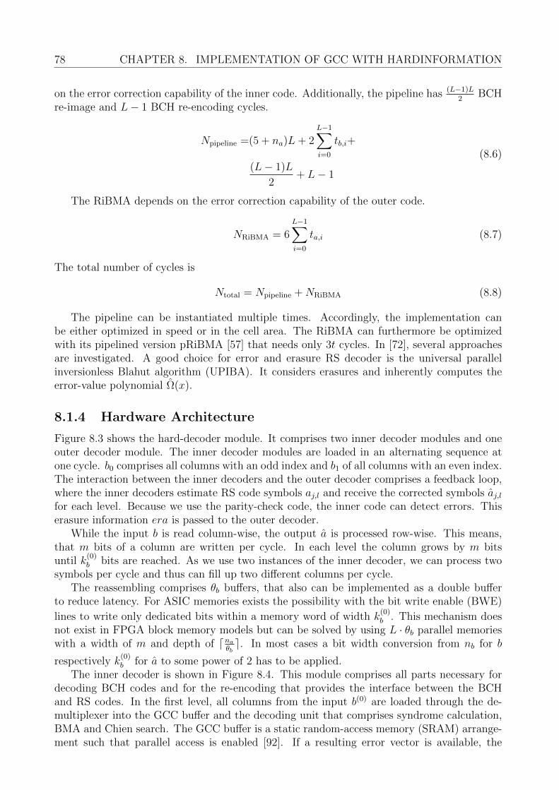
78 CHAPTER 8. IMPLEMENTATION OF GCC WITH HARDINFORMATION
on the error correction capability of the inner code. Additionally, the pipeline has (L−1)L2
BCHre-image and L− 1 BCH re-encoding cycles.
Npipeline =(5 + na)L+ 2L−1∑i=0
tb,i+
(L− 1)L
2+ L− 1
(8.6)
The RiBMA depends on the error correction capability of the outer code.
NRiBMA = 6L−1∑i=0
ta,i (8.7)
The total number of cycles is
Ntotal = Npipeline +NRiBMA (8.8)
The pipeline can be instantiated multiple times. Accordingly, the implementation canbe either optimized in speed or in the cell area. The RiBMA can furthermore be optimizedwith its pipelined version pRiBMA [57] that needs only 3t cycles. In [72], several approachesare investigated. A good choice for error and erasure RS decoder is the universal parallelinversionless Blahut algorithm (UPIBA). It considers erasures and inherently computes theerror-value polynomial Ω(x).
8.1.4 Hardware Architecture
Figure 8.3 shows the hard-decoder module. It comprises two inner decoder modules and oneouter decoder module. The inner decoder modules are loaded in an alternating sequence atone cycle. b0 comprises all columns with an odd index and b1 of all columns with an even index.The interaction between the inner decoders and the outer decoder comprises a feedback loop,where the inner decoders estimate RS code symbols aj,l and receive the corrected symbols aj,lfor each level. Because we use the parity-check code, the inner code can detect errors. Thiserasure information era is passed to the outer decoder.
While the input b is read column-wise, the output a is processed row-wise. This means,that m bits of a column are written per cycle. In each level the column grows by m bitsuntil k
(0)b bits are reached. As we use two instances of the inner decoder, we can process two
symbols per cycle and thus can fill up two different columns per cycle.The reassembling comprises θb buffers, that also can be implemented as a double buffer
to reduce latency. For ASIC memories exists the possibility with the bit write enable (BWE)
lines to write only dedicated bits within a memory word of width k(0)b . This mechanism does
not exist in FPGA block memory models but can be solved by using L · θb parallel memorieswith a width of m and depth of dna
θbe. In most cases a bit width conversion from nb for b
respectively k(0)b for a to some power of 2 has to be applied.
The inner decoder is shown in Figure 8.4. This module comprises all parts necessary fordecoding BCH codes and for the re-encoding that provides the interface between the BCHand RS codes. In the first level, all columns from the input b(0) are loaded through the de-multiplexer into the GCC buffer and the decoding unit that comprises syndrome calculation,BMA and Chien search. The GCC buffer is a static random-access memory (SRAM) arrange-ment such that parallel access is enabled [92]. If a resulting error vector is available, the
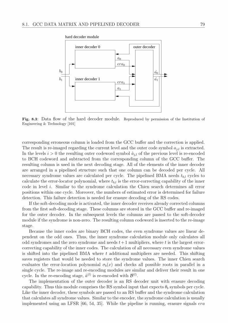
8.1. GCC DATA MATRIX AND PIPELINED DECODER 79
inner decoder 0
inner decoder 1
outer decoder
hard decoder module
b0
a0
a0
a1
a1
era0
era1b1
i
Fig. 8.3: Data flow of the hard decoder module. Reproduced by permission of the Institution ofEngineering & Technology [101]
corresponding erroneous column is loaded from the GCC buffer and the correction is applied.The result is re-imaged regarding the current level and the outer code symbol aj,l is extracted.In the levels i > 0 the resulting outer codeword symbol aj,l of the previous level is re-encodedto BCH codeword and subtracted from the corresponding column of the GCC buffer. Theresulting column is used in the next decoding stage. All of the elements of the inner decoderare arranged in a pipelined structure such that one column can be decoded per cycle. Allnecessary syndrome values are calculated per cycle. The pipelined BMA needs tb,l cycles tocalculate the error-locator polynomial, where tb,l is the error-correcting capability of the innercode in level i. Similar to the syndrome calculation the Chien search determines all errorpositions within one cycle. Moreover, the numbers of estimated error is determined for failuredetection. This failure detection is needed for erasure decoding of the RS codes.
If the soft-decoding mode is activated, the inner decoder receives already corrected columnsfrom the first soft-decoding stage. These columns are stored in the GCC buffer and re-imagedfor the outer decoder. In the subsequent levels the columns are passed to the soft-decodermodule if the syndrome is non-zero. The resulting column codeword is inserted to the re-imagestage.
Because the inner codes are binary BCH codes, the even syndrome values are linear de-pendent on the odd ones. Thus, the inner syndrome calculation module only calculates allodd syndromes and the zero syndrome and needs t+1 multipliers, where t is the largest error-correcting capability of the inner codes. The calculation of all necessary even syndrome valuesis shifted into the pipelined BMA where t additional multipliers are needed. This shiftingsaves registers that would be needed to store the syndrome values. The inner Chien searchevaluates the error-location polynomial σb(x) and checks all possible roots in parallel in asingle cycle. The re-image and re-encoding modules are similar and deliver their result in onecycle. In the re-encoding stage, a(l) is re-encoded with B(l).
The implementation of the outer decoder is an RS decoder unit with erasure decodingcapability. Thus this module comprises the RS symbol input that expects θb symbols per cycle.Like the inner decoder, these symbols are passed to an RS buffer and the syndrome calculationthat calculates all syndrome values. Similar to the encoder, the syndrome calculation is usuallyimplemented using an LFSR [66, 54, 35]. While the pipeline is running, erasure signals era
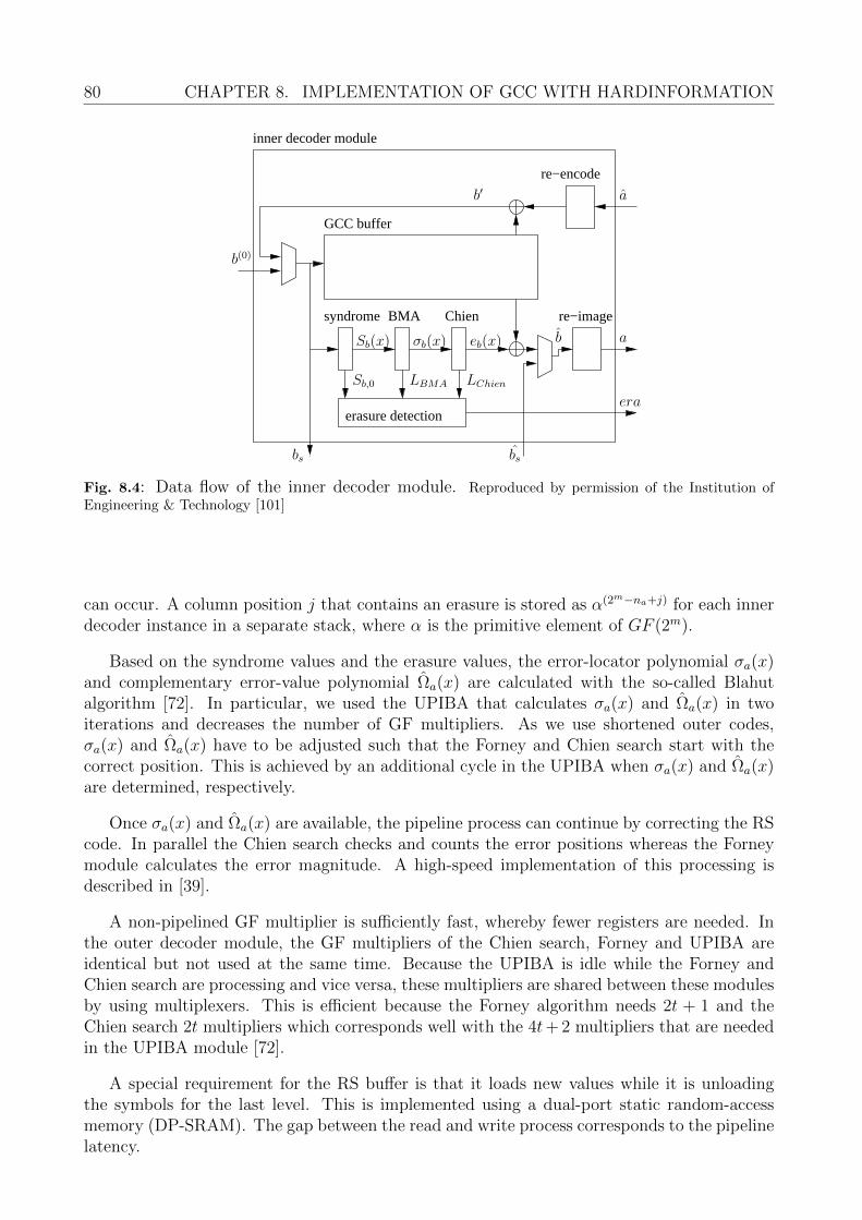
80 CHAPTER 8. IMPLEMENTATION OF GCC WITH HARDINFORMATION
BMA Chien
erasure detection
GCC buffer
inner decoder module
re−imagesyndrome
re−encode
LChien
bs
Sb(x) σb(x) eb(x)
LBMASb,0
b′ a
a
era
b
bs
b(0)
i
Fig. 8.4: Data flow of the inner decoder module. Reproduced by permission of the Institution ofEngineering & Technology [101]
can occur. A column position j that contains an erasure is stored as α(2m−na+j) for each innerdecoder instance in a separate stack, where α is the primitive element of GF (2m).
Based on the syndrome values and the erasure values, the error-locator polynomial σa(x)and complementary error-value polynomial Ωa(x) are calculated with the so-called Blahutalgorithm [72]. In particular, we used the UPIBA that calculates σa(x) and Ωa(x) in twoiterations and decreases the number of GF multipliers. As we use shortened outer codes,σa(x) and Ωa(x) have to be adjusted such that the Forney and Chien search start with thecorrect position. This is achieved by an additional cycle in the UPIBA when σa(x) and Ωa(x)are determined, respectively.
Once σa(x) and Ωa(x) are available, the pipeline process can continue by correcting the RScode. In parallel the Chien search checks and counts the error positions whereas the Forneymodule calculates the error magnitude. A high-speed implementation of this processing isdescribed in [39].
A non-pipelined GF multiplier is sufficiently fast, whereby fewer registers are needed. Inthe outer decoder module, the GF multipliers of the Chien search, Forney and UPIBA areidentical but not used at the same time. Because the UPIBA is idle while the Forney andChien search are processing and vice versa, these multipliers are shared between these modulesby using multiplexers. This is efficient because the Forney algorithm needs 2t + 1 and theChien search 2t multipliers which corresponds well with the 4t+ 2 multipliers that are neededin the UPIBA module [72].
A special requirement for the RS buffer is that it loads new values while it is unloadingthe symbols for the last level. This is implemented using a dual-port static random-accessmemory (DP-SRAM). The gap between the read and write process corresponds to the pipelinelatency.
8.2. CODEWORD BUFFER 81
outer decoder module
era
UPIBA
erasure stack
Chien−search
Forney
RS buffer
syndrome
a
a
0Sa(x)
σa(x)
σ′a(x)
Ωa(x)
i
Fig. 8.5: Data flow of the outer decoder module. Reproduced by permission of the Institution ofEngineering & Technology [101]
8.1.5 Encoder
The encoder performs two tasks: First each row is encoded with the desired RS code theneach column is encoded with the nested BCH code. At the beginning the data is loaded intothe RS encoder and simultaneously into the correct row of the GCC data matrix. Typically,the encoder is implemented as an LFSR where the coefficients of g(x) represent the taps of thefeedback [44, 66, 54, 35]. Because the GCC consists several RS codes, it comprises multipleLFSR instances. When finally a row is encoded the multiplexer switches to the next row.If all rows are encoded the GCC data matrix can be read column-wise while each column isencoded with the nested BCH code. Instead of using an LFSR the BCH encoders uses a directfull-parallel parity calculation.
8.2 Codeword Buffer
In this section, we describe an improvement of the GCC codeword buffer that was previouslydescribed by a shift register which has major impact on the die area of the ASIC implementa-tion. We first address the problem that comes from the flip-flop circuit shown in Figure 8.1.We show different solutions that can be made more efficient with SRAM modules. The mostefficient implementation will be described in further detail. Synthesis results can be found inSection 8.3.
Above a certain size, a register cell requires more area as a memory cell in an SRAM. Therequirements for the access of the GCC buffer are:
• column-wise access
• incremental addressing
• two read and one write access with constant column distances
We consider several SRAM constellations with different access mechanisms. There existssingle-port static random-access memorys (SP-SRAMs) where in each cycle only one single
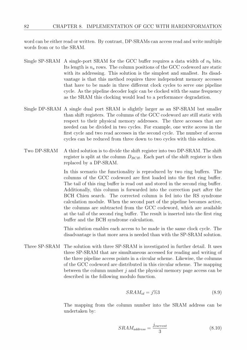
82 CHAPTER 8. IMPLEMENTATION OF GCC WITH HARDINFORMATION
word can be either read or written. By contrast, DP-SRAMs can access read and write multiplewords from or to the SRAM.
Single SP-SRAM A single-port SRAM for the GCC buffer requires a data width of nb bits.Its length is na rows. The column positions of the GCC codeword are staticwith its addressing. This solution is the simplest and smallest. Its disad-vantage is that this method requires three independent memory accessesthat have to be made in three different clock cycles to serve one pipelinecycle. As the pipeline decoder logic can be clocked with the same frequencyas the SRAM this clocking would lead to a performance degradation.
Single DP-SRAM A single dual port SRAM is slightly larger as an SP-SRAM but smallerthan shift registers. The columns of the GCC codeword are still static withrespect to their physical memory addresses. The three accesses that areneeded can be divided in two cycles. For example, one write access in thefirst cycle and two read accesses in the second cycle. The number of accesscycles can be reduced from three down to two cycles with this solution.
Two DP-SRAM A third solution is to divide the shift register into two DP-SRAM. The shiftregister is split at the column DBCH . Each part of the shift register is thenreplaced by a DP-SRAM.
In this scenario the functionality is reproduced by two ring buffers. Thecolumns of the GCC codeword are first loaded into the first ring buffer.The tail of this ring buffer is read out and stored in the second ring buffer.Additionally, this column is forwarded into the correction part after theBCH Chien search. The corrected column is fed into the RS syndromecalculation module. When the second part of the pipeline becomes active,the columns are subtracted from the GCC codeword, which are availableat the tail of the second ring buffer. The result is inserted into the first ringbuffer and the BCH syndrome calculation.
This solution enables each access to be made in the same clock cycle. Thedisadvantage is that more area is needed than with the SP-SRAM solution.
Three SP-SRAM The solution with three SP-SRAM is investigated in further detail. It usesthree SP-SRAM that are simultaneous accessed for reading and writing ofthe three pipeline access points in a circular scheme. Likewise, the columnsof the GCC codeword are distributed in this circular scheme. The mappingbetween the column number j and the physical memory page access can bedescribed in the following modulo function.
SRAMid = j%3 (8.9)
The mapping from the column number into the SRAM address can beundertaken by:
SRAMaddress =jcurrent
3(8.10)
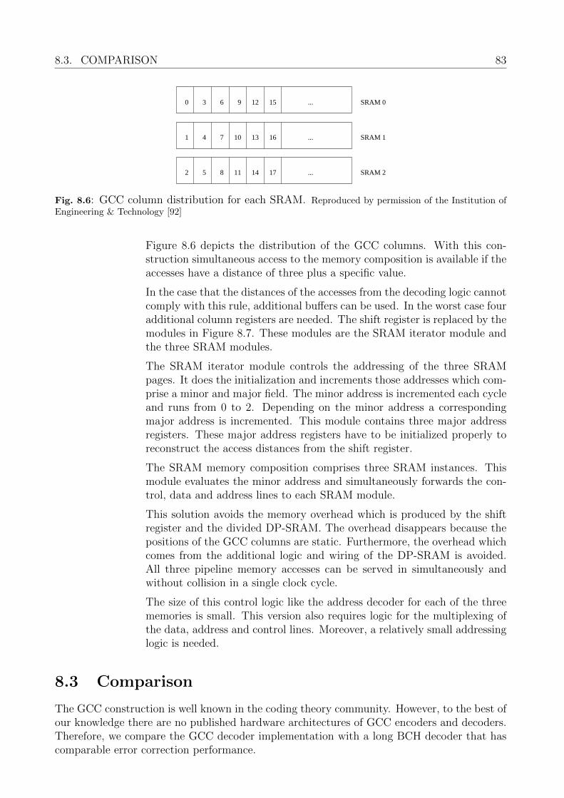
8.3. COMPARISON 83
0 3 6 9 ...12 15
...1 4 7 13 1610
...2 5 8 11 14 17
SRAM 0
SRAM 1
SRAM 2i
Fig. 8.6: GCC column distribution for each SRAM. Reproduced by permission of the Institution ofEngineering & Technology [92]
Figure 8.6 depicts the distribution of the GCC columns. With this con-struction simultaneous access to the memory composition is available if theaccesses have a distance of three plus a specific value.
In the case that the distances of the accesses from the decoding logic cannotcomply with this rule, additional buffers can be used. In the worst case fouradditional column registers are needed. The shift register is replaced by themodules in Figure 8.7. These modules are the SRAM iterator module andthe three SRAM modules.
The SRAM iterator module controls the addressing of the three SRAMpages. It does the initialization and increments those addresses which com-prise a minor and major field. The minor address is incremented each cycleand runs from 0 to 2. Depending on the minor address a correspondingmajor address is incremented. This module contains three major addressregisters. These major address registers have to be initialized properly toreconstruct the access distances from the shift register.
The SRAM memory composition comprises three SRAM instances. Thismodule evaluates the minor address and simultaneously forwards the con-trol, data and address lines to each SRAM module.
This solution avoids the memory overhead which is produced by the shiftregister and the divided DP-SRAM. The overhead disappears because thepositions of the GCC columns are static. Furthermore, the overhead whichcomes from the additional logic and wiring of the DP-SRAM is avoided.All three pipeline memory accesses can be served in simultaneously andwithout collision in a single clock cycle.
The size of this control logic like the address decoder for each of the threememories is small. This version also requires logic for the multiplexing ofthe data, address and control lines. Moreover, a relatively small addressinglogic is needed.
8.3 Comparison
The GCC construction is well known in the coding theory community. However, to the best ofour knowledge there are no published hardware architectures of GCC encoders and decoders.Therefore, we compare the GCC decoder implementation with a long BCH decoder that hascomparable error correction performance.
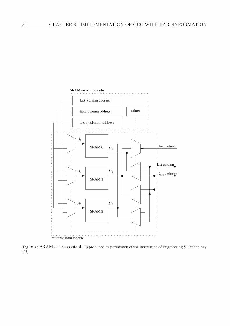
84 CHAPTER 8. IMPLEMENTATION OF GCC WITH HARDINFORMATION
SRAM 2
SRAM 1
SRAM 0
minor
first column
last column
last_column address
first_column address
multiple sram module
SRAM iterator module
Dbch column
Dbch column address
A0
A2
A1
D2
D0
D1
i
Fig. 8.7: SRAM access control. Reproduced by permission of the Institution of Engineering & Technology[92]
8.3. COMPARISON 85
Module Slacktime (ns)
BCH syndrome 4.66BCH iBMA 6.20BCH Chien search 8.80BCH re-image 8.67RS syndrome 7.87RS Chien search 7.39RS Forney alg. 4.52
RS RiBMA 5.26
Tab. 8.2: Slack time @100 MHz
The first example is an implementation of the proposed GCC code. First we describe thecode parameters which meet the constraints of FER and BER. Subsequently, we presentcell area size and clock frequency measurements. In the second example, a long BCH codeis presented, where we explain the code parameters and offer a brief overview of the decoderimplementation. Both decoders are implemented in Verilog and are synthesized with theDesign Compiler from Synopsys using a 40nm technology with high density standard cells(HVT + SVT).
Example 16. For the BCH code we use a 1-kByte information sector. The target FER of10−16 at ε = 3.8 ·10−3 requires a 96-bit-error-correcting BCH code. The long BCH code has theparameters A(214; 9609, 8280, t = 96). The implementation was synthesized with the same toolas in Example 4. In order to build a codeword with n = 9609 we need a Galois field GF (2m)with m = 14. This is a disadvantage as the complexity of a multiplier is O(m2) [18]. Theimplementation is based on a mixed serial/parallel implementation as proposed in [83].
The smaller Galois fields used in the GCC lead to a much smaller and faster implementationcompared to the BCH decoder with an arithmetic in GF (214). The BCH decoder achieves aclock frequency of 100 MHz. Table 8.2 shows the slack times for each module of the GCCdecoder. The first seven modules are the pipeline. The pipeline modules and the RS RiBMAcan be put in different clock domains. Using a common clock domain the GCC decoderachieves a clock frequency of 180 MHz.
From Equation (8.8) follows that the GCC implementation requires 2 286 cycles. Hence,the decoder achieves a throughput of 1.3 Gb/s, whereas the BCH decoder has a throughputof about 0.6 Gb/s. The worst slack times have the modules BCH syndrome and RS Forneyalgorithm. In the BCH syndrome module the shorter slack time comes from the calculationof the even syndrome values. These even syndrome values are calculated in the same cycle assquares or higher powers of odd syndrome values. As the iterative iBMA requires only thefirst syndrome value in the first instance, the calculation of the even syndrome values can bemoved in a later cycle without increasing the pipeline latency. Another bottleneck is the RSForney algorithm. Equation (3.18) shows that first Ω(x) and σ′(x) are evaluated. This needsa parallel multiplication and summation of all products. The final division leads to a secondmultiplication and causes the small slack time. In order to obtain a shorter critical path theForney algorithm can be divided into multiple cycles.
The cell area sizes for all modules are listed in Tab. 8.3, where we use a GE as a unit ofmeasure which is the area of a two-input drive-strength-one NAND gate. The decoder logicrequires 147 678 GE. Tab. 8.4 lists the cell area sizes for the BCH decoder logic. From thesevalues we observe that the logic of the GCC decoder requires only 30% of the cell area that isrequired for the BCH decoder.
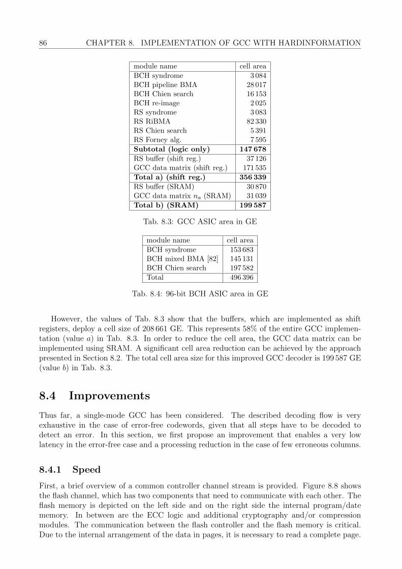
86 CHAPTER 8. IMPLEMENTATION OF GCC WITH HARDINFORMATION
module name cell area
BCH syndrome 3 084BCH pipeline BMA 28 017BCH Chien search 16 153BCH re-image 2 025RS syndrome 3 083RS RiBMA 82 330RS Chien search 5 391RS Forney alg. 7 595
Subtotal (logic only) 147 678
RS buffer (shift reg.) 37 126GCC data matrix (shift reg.) 171 535
Total a) (shift reg.) 356 339
RS buffer (SRAM) 30 870GCC data matrix na (SRAM) 31 039
Total b) (SRAM) 199 587
Tab. 8.3: GCC ASIC area in GE
module name cell area
BCH syndrome 153 683BCH mixed BMA [82] 145 131BCH Chien search 197 582
Total 496 396
Tab. 8.4: 96-bit BCH ASIC area in GE
However, the values of Tab. 8.3 show that the buffers, which are implemented as shiftregisters, deploy a cell size of 208 661 GE. This represents 58% of the entire GCC implemen-tation (value a) in Tab. 8.3. In order to reduce the cell area, the GCC data matrix can beimplemented using SRAM. A significant cell area reduction can be achieved by the approachpresented in Section 8.2. The total cell area size for this improved GCC decoder is 199 587 GE(value b) in Tab. 8.3.
8.4 Improvements
Thus far, a single-mode GCC has been considered. The described decoding flow is veryexhaustive in the case of error-free codewords, given that all steps have to be decoded todetect an error. In this section, we first propose an improvement that enables a very lowlatency in the error-free case and a processing reduction in the case of few erroneous columns.
8.4.1 Speed
First, a brief overview of a common controller channel stream is provided. Figure 8.8 showsthe flash channel, which has two components that need to communicate with each other. Theflash memory is depicted on the left side and on the right side the internal program/datememory. In between are the ECC logic and additional cryptography and/or compressionmodules. The communication between the flash controller and the flash memory is critical.Due to the internal arrangement of the data in pages, it is necessary to read a complete page.
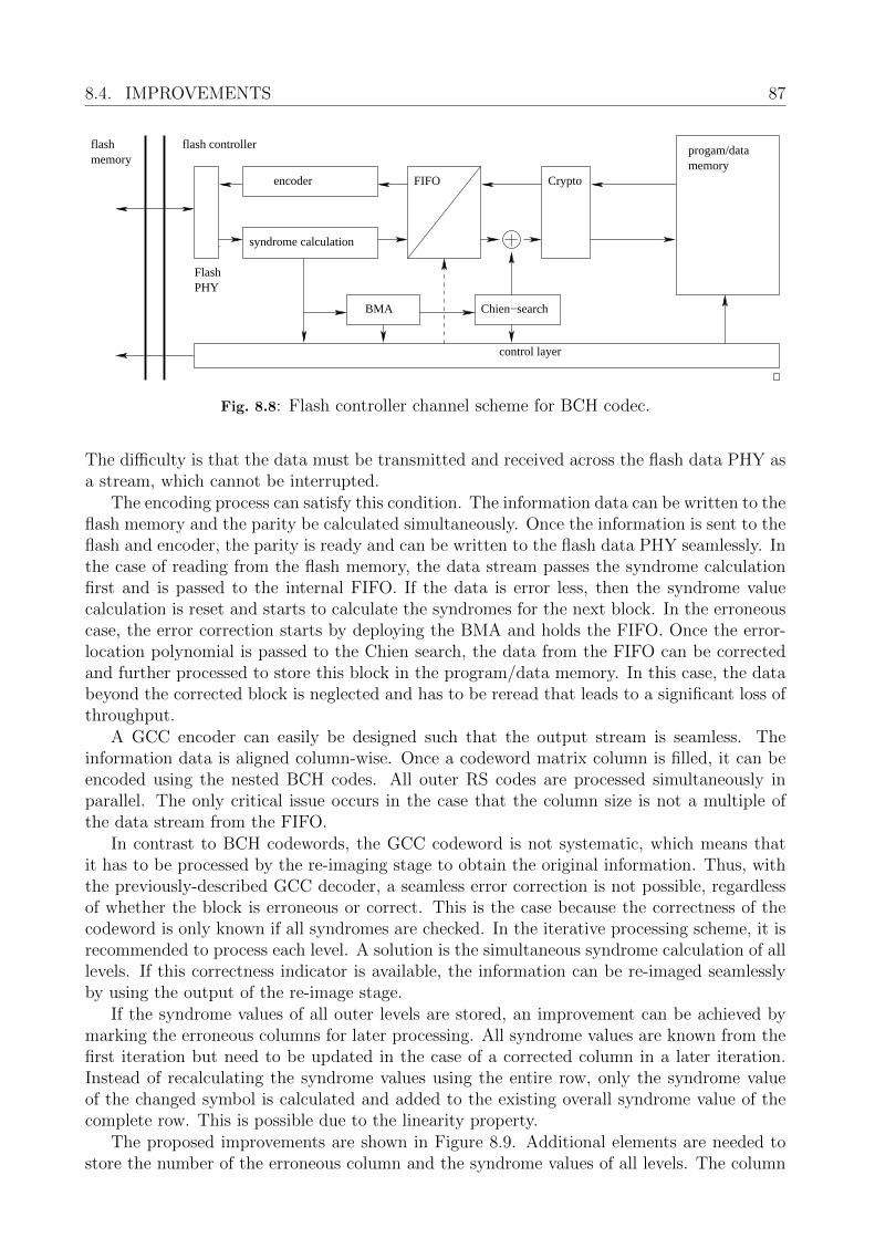
8.4. IMPROVEMENTS 87
BMA
syndrome calculation
encoder FIFO
Chien−search
flashmemory
FlashPHY
Crypto
control layer
progam/datamemory
flash controller
i
Fig. 8.8: Flash controller channel scheme for BCH codec.
The difficulty is that the data must be transmitted and received across the flash data PHY asa stream, which cannot be interrupted.
The encoding process can satisfy this condition. The information data can be written to theflash memory and the parity be calculated simultaneously. Once the information is sent to theflash and encoder, the parity is ready and can be written to the flash data PHY seamlessly. Inthe case of reading from the flash memory, the data stream passes the syndrome calculationfirst and is passed to the internal FIFO. If the data is error less, then the syndrome valuecalculation is reset and starts to calculate the syndromes for the next block. In the erroneouscase, the error correction starts by deploying the BMA and holds the FIFO. Once the error-location polynomial is passed to the Chien search, the data from the FIFO can be correctedand further processed to store this block in the program/data memory. In this case, the databeyond the corrected block is neglected and has to be reread that leads to a significant loss ofthroughput.
A GCC encoder can easily be designed such that the output stream is seamless. Theinformation data is aligned column-wise. Once a codeword matrix column is filled, it can beencoded using the nested BCH codes. All outer RS codes are processed simultaneously inparallel. The only critical issue occurs in the case that the column size is not a multiple ofthe data stream from the FIFO.
In contrast to BCH codewords, the GCC codeword is not systematic, which means thatit has to be processed by the re-imaging stage to obtain the original information. Thus, withthe previously-described GCC decoder, a seamless error correction is not possible, regardlessof whether the block is erroneous or correct. This is the case because the correctness of thecodeword is only known if all syndromes are checked. In the iterative processing scheme, it isrecommended to process each level. A solution is the simultaneous syndrome calculation of alllevels. If this correctness indicator is available, the information can be re-imaged seamlesslyby using the output of the re-image stage.
If the syndrome values of all outer levels are stored, an improvement can be achieved bymarking the erroneous columns for later processing. All syndrome values are known from thefirst iteration but need to be updated in the case of a corrected column in a later iteration.Instead of recalculating the syndrome values using the entire row, only the syndrome valueof the changed symbol is calculated and added to the existing overall syndrome value of thecomplete row. This is possible due to the linearity property.
The proposed improvements are shown in Figure 8.9. Additional elements are needed tostore the number of the erroneous column and the syndrome values of all levels. The column
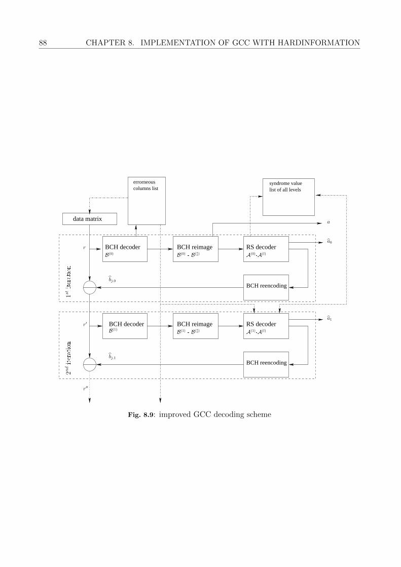
88 CHAPTER 8. IMPLEMENTATION OF GCC WITH HARDINFORMATION
BCH reimage RS decoder
BCH reencoding
BCH reencoding
RS decoderBCH reimageBCH decoder
BCH decoder
data matrix
errorneouscolumns list list of all levels
syndrome value
1st
i
t
e
r
a
t
i
o
n
2nd
i
t
e
r
a
t
i
o
n
r
r′
r′′
bj.1
bj.0
B(0)
a0
a1
B(1)
B(0)- B(l)
a
B(1)- B(l)
A(0)-A(l)
A(1)-A(l)
i
Fig. 8.9: improved GCC decoding scheme
8.5. SUMMARY 89
number is used to load and decode only the erroneous columns and as the coefficient for theouter syndrome calculation.
8.5 Summary
In this chapter, we have shown how the GCC decoding described in Chapter 4 can be im-plemented in hardware. Based on the decoding scheme shown in Figure 4.7, we derived adata flow shown in Figure 8.1, which is the draft for the hardware modules and offers a firstoverview of the necessary calculation and buffers. From that point, the hardware moduleswere designed as depicted in Figures 8.3, 8.4 and 8.5. It is clear that the GCC codewordbuffer depicted in 8.1 is not suitable to be implemented as a shift register due to the largearea. Instead, an alternative buffer was developed. This was possible due to the sequence ofcolumn codes that are read. This GCC implementation then was compared to a BCH. Bydividing a large algebraic code into several smaller ones the complexity was reduced mainlythrough the GF arithmetic. The GCC then led to a higher code rate. It also shows that anaccurate comparison is difficult due to design criteria like achievable throughput, code rate ordecoding performance.
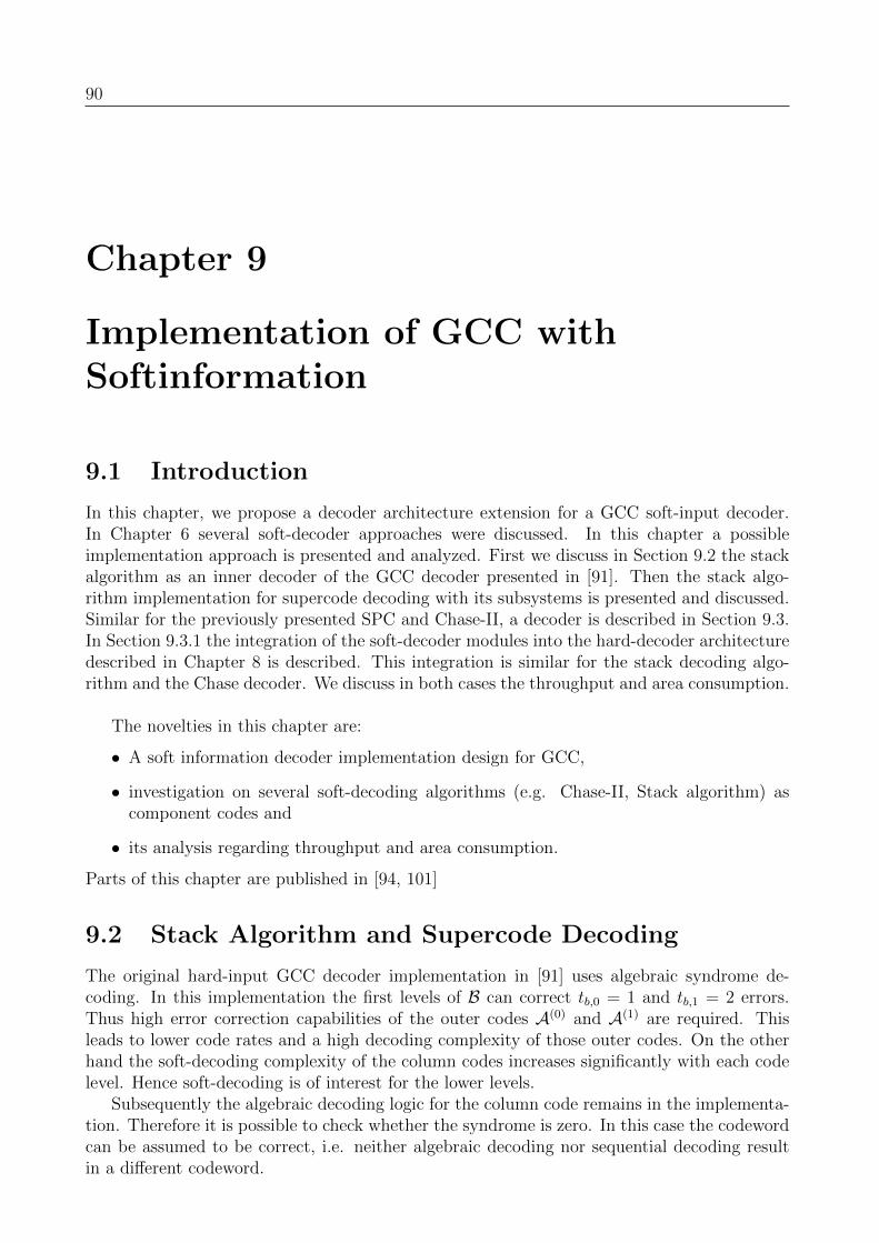
90
Chapter 9
Implementation of GCC withSoftinformation
9.1 Introduction
In this chapter, we propose a decoder architecture extension for a GCC soft-input decoder.In Chapter 6 several soft-decoder approaches were discussed. In this chapter a possibleimplementation approach is presented and analyzed. First we discuss in Section 9.2 the stackalgorithm as an inner decoder of the GCC decoder presented in [91]. Then the stack algo-rithm implementation for supercode decoding with its subsystems is presented and discussed.Similar for the previously presented SPC and Chase-II, a decoder is described in Section 9.3.In Section 9.3.1 the integration of the soft-decoder modules into the hard-decoder architecturedescribed in Chapter 8 is described. This integration is similar for the stack decoding algo-rithm and the Chase decoder. We discuss in both cases the throughput and area consumption.
The novelties in this chapter are:
• A soft information decoder implementation design for GCC,
• investigation on several soft-decoding algorithms (e.g. Chase-II, Stack algorithm) ascomponent codes and
• its analysis regarding throughput and area consumption.
Parts of this chapter are published in [94, 101]
9.2 Stack Algorithm and Supercode Decoding
The original hard-input GCC decoder implementation in [91] uses algebraic syndrome de-coding. In this implementation the first levels of B can correct tb,0 = 1 and tb,1 = 2 errors.Thus high error correction capabilities of the outer codes A(0) and A(1) are required. Thisleads to lower code rates and a high decoding complexity of those outer codes. On the otherhand the soft-decoding complexity of the column codes increases significantly with each codelevel. Hence soft-decoding is of interest for the lower levels.
Subsequently the algebraic decoding logic for the column code remains in the implementa-tion. Therefore it is possible to check whether the syndrome is zero. In this case the codewordcan be assumed to be correct, i.e. neither algebraic decoding nor sequential decoding resultin a different codeword.
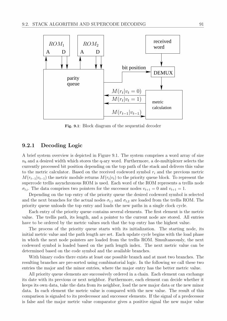
9.2. STACK ALGORITHM AND SUPERCODE DECODING 91
parityqueue
metriccalculation
A D A D
bit positionDEMUX
receivedword
ROM1 ROM2
M(rt|vt = 0)
M(rt|vt = 1)
M(rt−1|vt−1)i
Fig. 9.1: Block diagram of the sequential decoder
9.2.1 Decoding Logic
A brief system overview is depicted in Figure 9.1. The system comprises a word array of sizenb and a desired width which stores the q-ary word. Furthermore, a de-multiplexer selects thecurrently processed bit position depending on the top path of the stack and delivers this valueto the metric calculator. Based on the received codeword symbol ri and the previous metricM(rt−1|vt−1) the metric module returns M(rt|vt) to the priority queue block. To represent thesupercode trellis asynchronous ROM is used. Each word of the ROM represents a trellis nodeσt,i. The data comprises two pointers for the successor nodes vt+1 = 0 and vt+1 = 1.
Depending on the top entry of the priority queue the desired codeword symbol is selectedand the next branches for the actual nodes σt,1 and σt,2 are loaded from the trellis ROM. Thepriority queue unloads the top entry and loads the new paths in a single clock cycle.
Each entry of the priority queue contains several elements. The first element is the metricvalue. The trellis path, its length, and a pointer to the current node are stored. All entrieshave to be ordered by the metric values such that the top entry has the highest value.
The process of the priority queue starts with its initialization. The starting node, itsinitial metric value and the path length are set. Each update cycle begins with the load phasein which the next node pointers are loaded from the trellis ROM. Simultaneously, the nextcodeword symbol is loaded based on the path length index. The next metric value can bedetermined based on the code symbol and the available branches.
With binary codes there exists at least one possible branch and at most two branches. Theresulting branches are pre-sorted using combinatorial logic. In the following we call these twoentries the major and the minor entries, where the major entry has the better metric value.
All priority queue elements are successively ordered in a chain. Each element can exchangeits date with its previous or next neighbor. Furthermore, each element can decide whether itkeeps its own data, take the data from its neighbor, load the new major data or the new minordata. In each element the metric value is compared with the new value. The result of thiscomparison is signaled to its predecessor and successor elements. If the signal of a predecessoris false and the major metric value comparator gives a positive signal the new major value
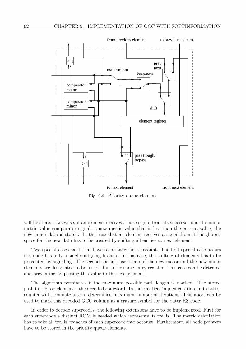
92 CHAPTER 9. IMPLEMENTATION OF GCC WITH SOFTINFORMATION
comparatorminor
majorcomparator
element register
bypass
shift
prevnext
keep/newmajor/minor
to previous elementfrom previous element
to next element from next element
pass trough/
≥ 1
≥ 1
i
Fig. 9.2: Priority queue element
will be stored. Likewise, if an element receives a false signal from its successor and the minormetric value comparator signals a new metric value that is less than the current value, thenew minor data is stored. In the case that an element receives a signal from its neighbors,space for the new data has to be created by shifting all entries to next element.
Two special cases exist that have to be taken into account. The first special case occursif a node has only a single outgoing branch. In this case, the shifting of elements has to beprevented by signaling. The second special case occurs if the new major and the new minorelements are designated to be inserted into the same entry register. This case can be detectedand preventing by passing this value to the next element.
The algorithm terminates if the maximum possible path length is reached. The storedpath in the top element is the decoded codeword. In the practical implementation an iterationcounter will terminate after a determined maximum number of iterations. This abort can beused to mark this decoded GCC column as a erasure symbol for the outer RS code.
In order to decode supercodes, the following extensions have to be implemented. First foreach supercode a distinct ROM is needed which represents its trellis. The metric calculationhas to take all trellis branches of each supercode into account. Furthermore, all node pointershave to be stored in the priority queue elements.

9.2. STACK ALGORITHM AND SUPERCODE DECODING 93
Eb/N
0 [dB]
4 4.5 5 5.5 6 6.5 7 7.5 8
num
ber
of d
ecod
ing
cycl
es
0
20
40
60
80
100
120
140
1st level2nd level
i
Fig. 9.3: Average number of iterations for the first and second level
9.2.2 Area Comparison and Throughput Estimation
In this section, we present an FPGA implementation of the proposed soft-input decoder andcompare it with the hard-input decoder presented in [91]. The hard-input decoder uses al-gebraic decoding. It comprises of the syndrome calculation, the BMA, and the Chien searchmodule. The soft input decoder is implemented as proposed in Section 6.1.2. It has twolimitations. First, the length of the priority queue is limited to 64 elements. Furthermore, theaccuracy of the metric calculation is limited to sixteen bits, and we use three-bit quantizationof the input symbols.
The stack algorithm has a variable execution time depending on the error pattern. Thisalgorithm needs at least 61 cycles to traverse the entire trellis if no error occurred. This casecan be omitted by checking whether the syndrome of a column word is zero. If no error isdetected the soft-decoding can be avoided and thus only a single cycle is needed.
Figure 9.3 depicts the average number of cycles needed for the stack algorithm. It showsthe dependency between the channel bit error rate and the computational complexity, i.e.fewer errors lead to fewer decoding cycles. Note that the algebraic hard-input decoder needsfour cycles for the first and six cycles for the second level. Hence, for high SNR ratios the stackalgorithm requires an average number of cycles that is comparable with hard-input decoding.
Next we present FPGA synthesis result for the stack algorithm. The synthesis was per-formed with Xilinx Vivado and a Virtex-7 target device. Table 9.1 shows the number ofslices and look-up tables (LUT) of the hard- and soft-input decoder with three-bit quantiza-tion. From these results we observe that the number of logic elements required for the stackalgorithm is about 82% of the number of logic gates required for the GCC hard-input decoder.
94 CHAPTER 9. IMPLEMENTATION OF GCC WITH SOFTINFORMATION
Module LUT SlicesRS module (t=78)Syndrome 1 701 1 395BMA 21 701 6 662Forney alg. 1 046 729Chien search 854 712BCH Module (n=60,t=8)Syndrome 184 46BMA 2 006 732Chien search 1 557 240re-image 148 336Total 29 197 10 852Stack alg. 23 896 9 885
Tab. 9.1: Results of an FPGA synthesis
9.2.3 Concluding Remarks and Future Directions
In this section, we have presented a soft input decoder for generalized concatenated codes.We have proposed a sequential decoding algorithm based on supercode trellises to reducethe complexity of the soft-input decoding compared to ordinary trellis based decoding. Thisimplementation improves the error correction capability significantly compared with hard-input decoding. Consequently, the proposed method is a promising approach for soft-inputdecoding of GCC. The implementation of the stack algorithm is nine times large than thealgebraic decoder. This complexity can be reduced by moving the majority of the registerentries into read only memory. Nevertheless, the proposed soft-input decoding increases theoverall complexity of the GCC decoder by 82% compared to the decoder presented in [92].Other soft-input decoding methods for binary BCH codes may reduce the overall decodingcomplexity.
The proposed coding scheme is well suited for applications that require very low residualerror rates, e.g. it might be appropriate for flash memories that provide soft informationabout the state of the memory cells. For flash memories, various concatenated coding schemeswere proposed to enable soft-input decoding, e.g. product codes [75] and concatenated codingschemes based on trellis coded modulation and outer BCH oder RS codes [64, 41, 55]. For thepresented simulation results we assumed a quantized additive white Gaussian noise channel.For practical flash memories, this model is not accurate. With multi-level cell and triple-levelcell technologies, the reliability of the bit levels and cells varies and coding schemes wereproposed that take these error characteristics into account [74, 73, 27, 26]. We believe thatthe adaptation of the proposed GCC coding scheme for flash memories is a promising directionfor further research.
9.3 Chase Decoder
At this point we discuss the alternative to the stack decoding algorithm as mentioned inChapter 6. In this scenario a SPC, a special case of the Chase algorithm, is applied in thefirst decoding level. The second and third levels are decoded using the Chase-II decoder.
The LLR values comprise one bit representing the sign and four bits that indicate thereliability. The least reliable bit position is determined by a sorting stage for the LLR values as
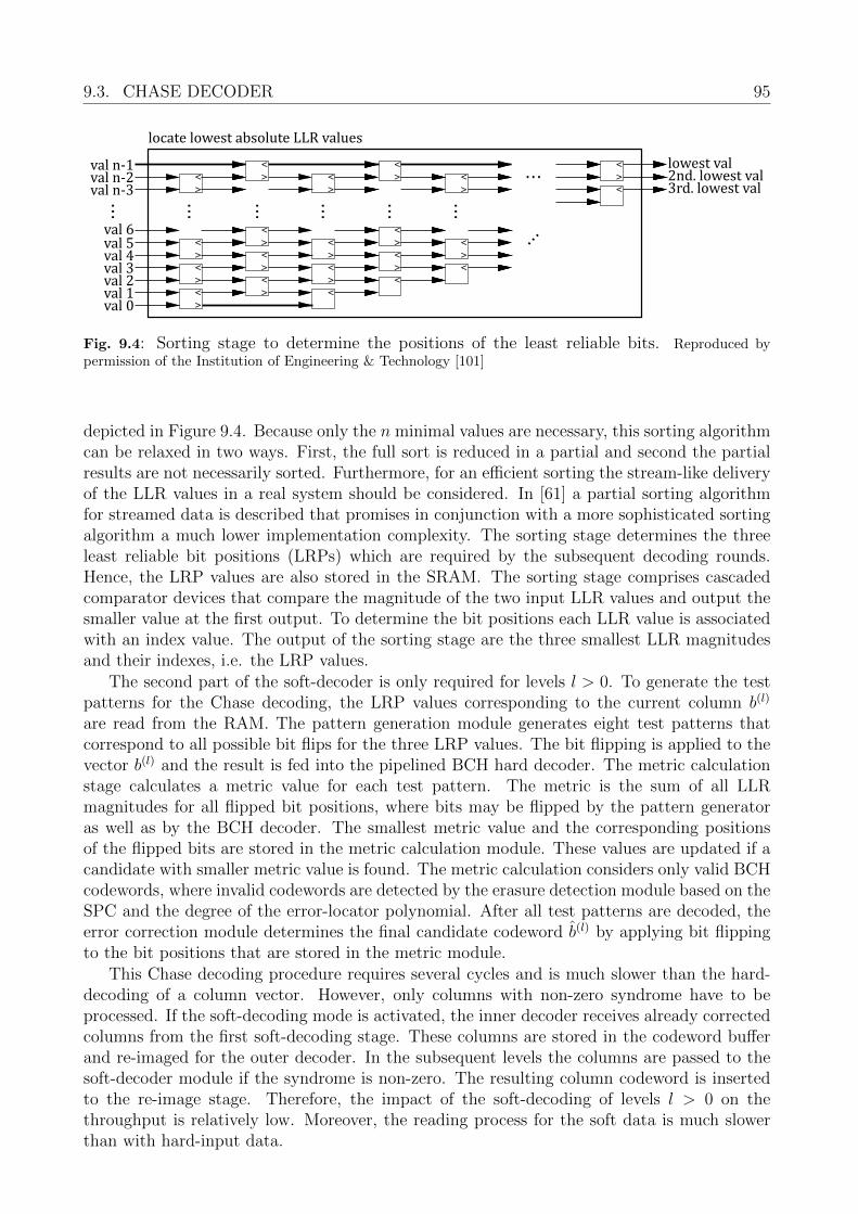
9.3. CHASE DECODER 95
locate lowest absolute LLR values
<
>
<
>
<
>
<
>
<
>
<
>
<
<
>
<
>
<
<
>
<
>
<
<
>
<
>
<
> <
>
<
> <
> <
<
>...
...
...
...
...
...
...
val 0 val 1 val 2 val 3 val 4 val 5
val 6
val n-3 val n-2 val n-1
3rd. lowest val 2nd. lowest val lowest val
...
i
Fig. 9.4: Sorting stage to determine the positions of the least reliable bits. Reproduced bypermission of the Institution of Engineering & Technology [101]
depicted in Figure 9.4. Because only the n minimal values are necessary, this sorting algorithmcan be relaxed in two ways. First, the full sort is reduced in a partial and second the partialresults are not necessarily sorted. Furthermore, for an efficient sorting the stream-like deliveryof the LLR values in a real system should be considered. In [61] a partial sorting algorithmfor streamed data is described that promises in conjunction with a more sophisticated sortingalgorithm a much lower implementation complexity. The sorting stage determines the threeleast reliable bit positions (LRPs) which are required by the subsequent decoding rounds.Hence, the LRP values are also stored in the SRAM. The sorting stage comprises cascadedcomparator devices that compare the magnitude of the two input LLR values and output thesmaller value at the first output. To determine the bit positions each LLR value is associatedwith an index value. The output of the sorting stage are the three smallest LLR magnitudesand their indexes, i.e. the LRP values.
The second part of the soft-decoder is only required for levels l > 0. To generate the testpatterns for the Chase decoding, the LRP values corresponding to the current column b(l)
are read from the RAM. The pattern generation module generates eight test patterns thatcorrespond to all possible bit flips for the three LRP values. The bit flipping is applied to thevector b(l) and the result is fed into the pipelined BCH hard decoder. The metric calculationstage calculates a metric value for each test pattern. The metric is the sum of all LLRmagnitudes for all flipped bit positions, where bits may be flipped by the pattern generatoras well as by the BCH decoder. The smallest metric value and the corresponding positionsof the flipped bits are stored in the metric calculation module. These values are updated if acandidate with smaller metric value is found. The metric calculation considers only valid BCHcodewords, where invalid codewords are detected by the erasure detection module based on theSPC and the degree of the error-locator polynomial. After all test patterns are decoded, theerror correction module determines the final candidate codeword b(l) by applying bit flippingto the bit positions that are stored in the metric module.
This Chase decoding procedure requires several cycles and is much slower than the hard-decoding of a column vector. However, only columns with non-zero syndrome have to beprocessed. If the soft-decoding mode is activated, the inner decoder receives already correctedcolumns from the first soft-decoding stage. These columns are stored in the codeword bufferand re-imaged for the outer decoder. In the subsequent levels the columns are passed to thesoft-decoder module if the syndrome is non-zero. The resulting column codeword is insertedto the re-image stage. Therefore, the impact of the soft-decoding of levels l > 0 on thethroughput is relatively low. Moreover, the reading process for the soft data is much slowerthan with hard-input data.
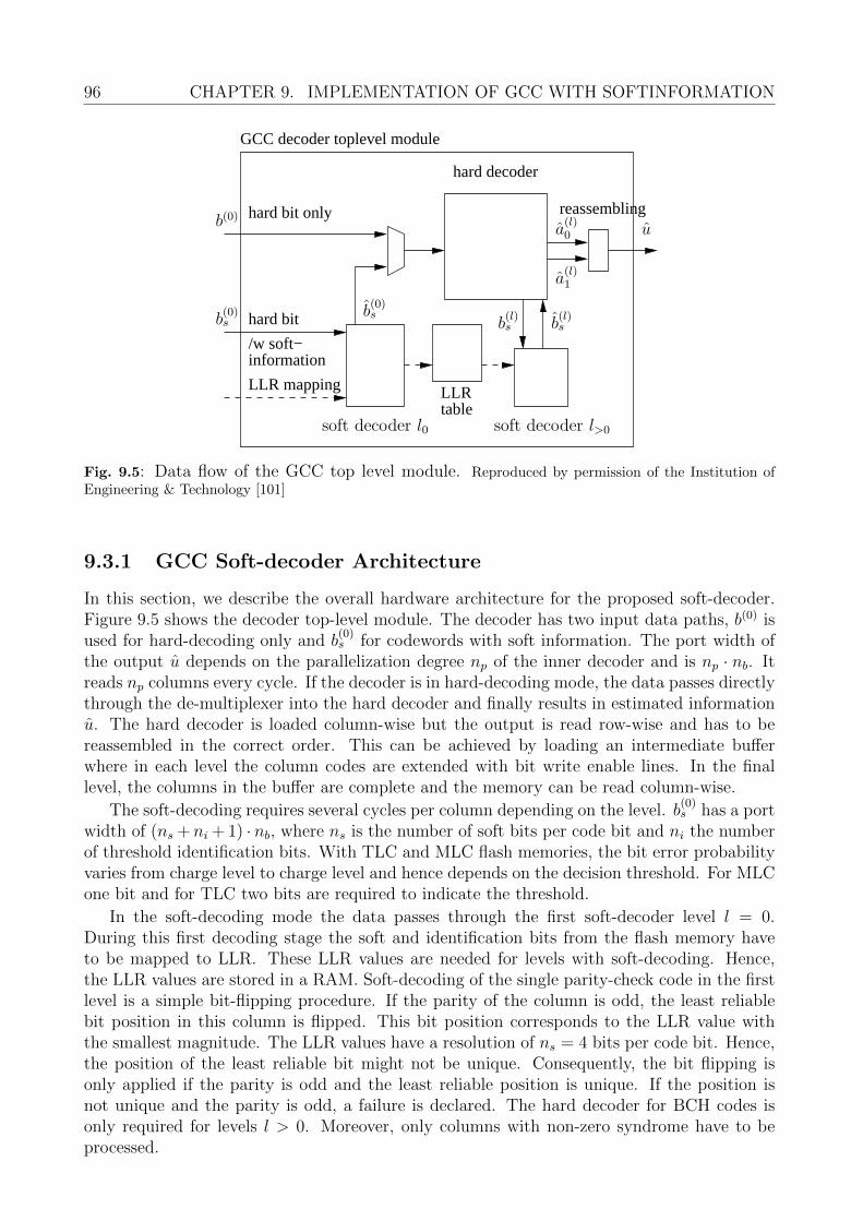
96 CHAPTER 9. IMPLEMENTATION OF GCC WITH SOFTINFORMATION
hard bit only
hard bit
/w soft−information
LLR mapping
reassembling
hard decoder
LLRtable
GCC decoder toplevel module
u
soft decoder l0 soft decoder l>0
b(0)s
b(l)s
a(l)1
a(l)0
b(0)s
b(0)
b(l)s
i
Fig. 9.5: Data flow of the GCC top level module. Reproduced by permission of the Institution ofEngineering & Technology [101]
9.3.1 GCC Soft-decoder Architecture
In this section, we describe the overall hardware architecture for the proposed soft-decoder.Figure 9.5 shows the decoder top-level module. The decoder has two input data paths, b(0) isused for hard-decoding only and b
(0)s for codewords with soft information. The port width of
the output u depends on the parallelization degree np of the inner decoder and is np · nb. Itreads np columns every cycle. If the decoder is in hard-decoding mode, the data passes directlythrough the de-multiplexer into the hard decoder and finally results in estimated informationu. The hard decoder is loaded column-wise but the output is read row-wise and has to bereassembled in the correct order. This can be achieved by loading an intermediate bufferwhere in each level the column codes are extended with bit write enable lines. In the finallevel, the columns in the buffer are complete and the memory can be read column-wise.
The soft-decoding requires several cycles per column depending on the level. b(0)s has a port
width of (ns + ni + 1) · nb, where ns is the number of soft bits per code bit and ni the numberof threshold identification bits. With TLC and MLC flash memories, the bit error probabilityvaries from charge level to charge level and hence depends on the decision threshold. For MLCone bit and for TLC two bits are required to indicate the threshold.
In the soft-decoding mode the data passes through the first soft-decoder level l = 0.During this first decoding stage the soft and identification bits from the flash memory haveto be mapped to LLR. These LLR values are needed for levels with soft-decoding. Hence,the LLR values are stored in a RAM. Soft-decoding of the single parity-check code in the firstlevel is a simple bit-flipping procedure. If the parity of the column is odd, the least reliablebit position in this column is flipped. This bit position corresponds to the LLR value withthe smallest magnitude. The LLR values have a resolution of ns = 4 bits per code bit. Hence,the position of the least reliable bit might not be unique. Consequently, the bit flipping isonly applied if the parity is odd and the least reliable position is unique. If the position isnot unique and the parity is odd, a failure is declared. The hard decoder for BCH codes isonly required for levels l > 0. Moreover, only columns with non-zero syndrome have to beprocessed.
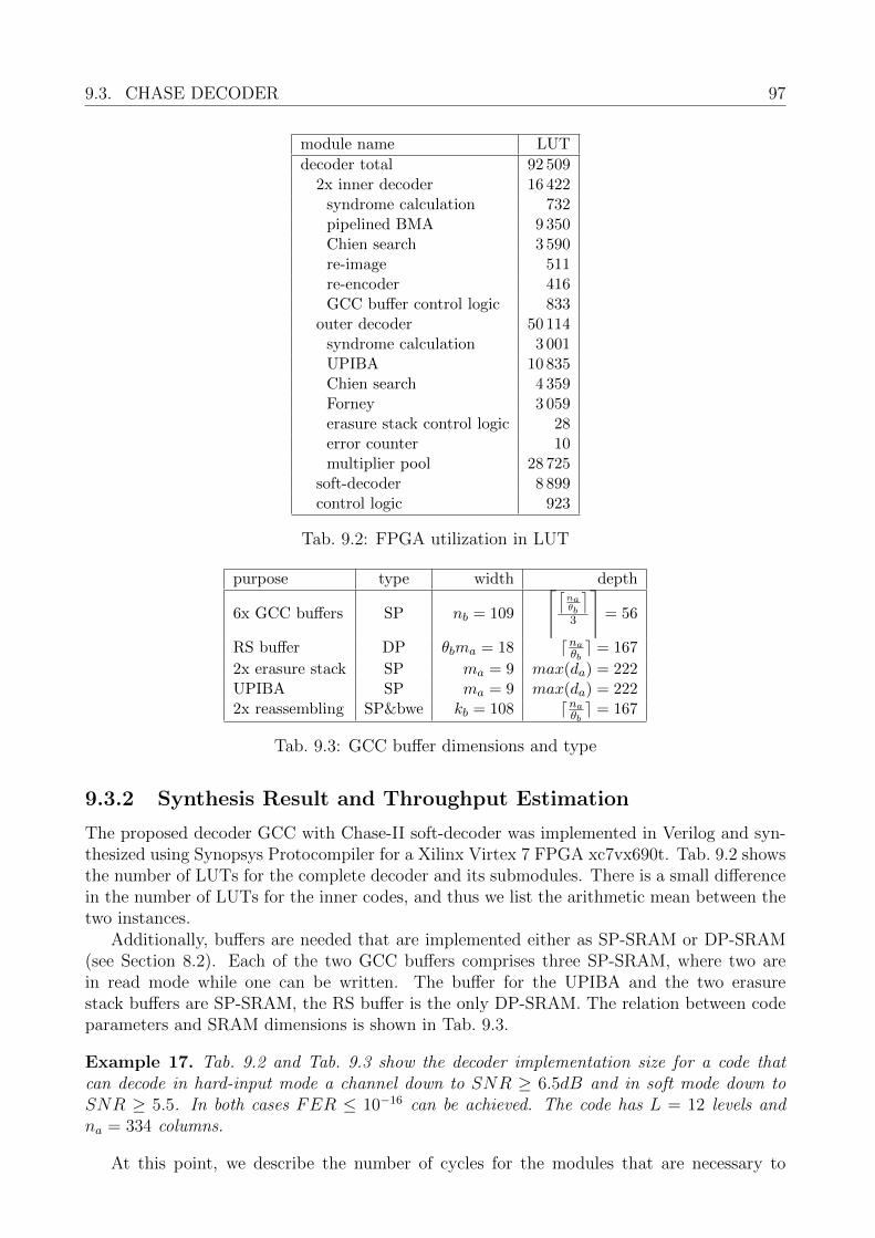
9.3. CHASE DECODER 97
module name LUT
decoder total 92 5092x inner decoder 16 422
syndrome calculation 732pipelined BMA 9 350Chien search 3 590re-image 511re-encoder 416GCC buffer control logic 833
outer decoder 50 114syndrome calculation 3 001UPIBA 10 835Chien search 4 359Forney 3 059erasure stack control logic 28error counter 10multiplier pool 28 725
soft-decoder 8 899control logic 923
Tab. 9.2: FPGA utilization in LUT
purpose type width depth
6x GCC buffers SP nb = 109
⌈⌈naθb
⌉3
⌉= 56
RS buffer DP θbma = 18 dnaθb e = 167
2x erasure stack SP ma = 9 max(da) = 222UPIBA SP ma = 9 max(da) = 2222x reassembling SP&bwe kb = 108 dnaθb e = 167
Tab. 9.3: GCC buffer dimensions and type
9.3.2 Synthesis Result and Throughput Estimation
The proposed decoder GCC with Chase-II soft-decoder was implemented in Verilog and syn-thesized using Synopsys Protocompiler for a Xilinx Virtex 7 FPGA xc7vx690t. Tab. 9.2 showsthe number of LUTs for the complete decoder and its submodules. There is a small differencein the number of LUTs for the inner codes, and thus we list the arithmetic mean between thetwo instances.
Additionally, buffers are needed that are implemented either as SP-SRAM or DP-SRAM(see Section 8.2). Each of the two GCC buffers comprises three SP-SRAM, where two arein read mode while one can be written. The buffer for the UPIBA and the two erasurestack buffers are SP-SRAM, the RS buffer is the only DP-SRAM. The relation between codeparameters and SRAM dimensions is shown in Tab. 9.3.
Example 17. Tab. 9.2 and Tab. 9.3 show the decoder implementation size for a code thatcan decode in hard-input mode a channel down to SNR ≥ 6.5dB and in soft mode down toSNR ≥ 5.5. In both cases FER ≤ 10−16 can be achieved. The code has L = 12 levels andna = 334 columns.
At this point, we describe the number of cycles for the modules that are necessary to
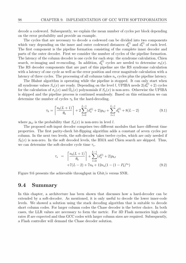
98 CHAPTER 9. IMPLEMENTATION OF GCC WITH SOFTINFORMATION
decode a codeword. Subsequently, we explain the mean number of cycles per block dependingon the error probability and provide an example.
The cycles that are necessary to decode a codeword can be divided into two componentswhich vary depending on the inner and outer codeword distances d
(l)b and d
(l)a of each level.
The first component is the pipeline formation consisting of the complete inner decoder andparts of the outer decoder. First we consider the number of cycles of the pipeline formation.The latency of the column decoder is one cycle for each step: the syndrome calculation, Chiensearch, re-imaging and re-encoding. In addition, d
(l)b cycles are needed to determine σb(x).
The RS decoder components that are part of this pipeline are the RS syndrome calculationwith a latency of one cycle as well as the error position and error magnitude calculation with alatency of three cycles. The processing of all columns takes na cycles plus the pipeline latency.
The Blahut algorithm is operating while the pipeline is stopped. It can only start whenall syndrome values Sa(x) are ready. Depending on the level l, UPIBA needs 2(d
(l)a + 2) cycles
for the calculation of σa(x) and Ωa(x) polynomials if Sa(x) is non-zero. Otherwise the UPIBAis skipped and the pipeline process is continued seamlessly. Based on this estimation we candetermine the number of cycles τh for the hard-decoding.
τh =
⌈nb(L+ 1)
θb
⌉+ 2
L−1∑l=0
(d(l)a + 2)pb,l +
L−1∑l=1
d(l)b + 8(L− 2) (9.1)
where pb,l is the probability that Sa(x) is non-zero in level l.The proposed soft-input decoder comprises two different modules that have different time
properties. The first parity-check bit-flipping algorithm adds a constant of seven cycles percolumn. In the next two levels, the soft-decoder takes twelve cycles, which are only needed ifSb(x) is non-zero. In the soft decoded levels, the BMA and Chien search are skipped. Thus,we can determine the soft-decoder cycle time τs.
τs =
⌈nb(L+ 1)
θb
⌉+
L−1∑l=0
(d(l)a + 2)pb,l
+7(L− 2) + 7nb + 12na(1− (1− Pb)nb) (9.2)
Figure 9.6 presents the achievable throughput in Gbit/s versus SNR.
9.4 Summary
In this chapter, a architecture has been shown that discusses how a hard-decoder can beextended by a soft-decoder. As mentioned, it is only useful to decode the lower inner-codelevels. We showed a solution using the stack decoding algorithm that is suitable to decodeshort column codes. For larger column codes the Chase decoder is the better choice. In bothcases, the LLR values are necessary to form the metric. For 3D Flash memories high coderates R are expected and thus GCC codes with larger column sizes are required. Subsequently,a Flash controller will demand the Chase decoder solution.
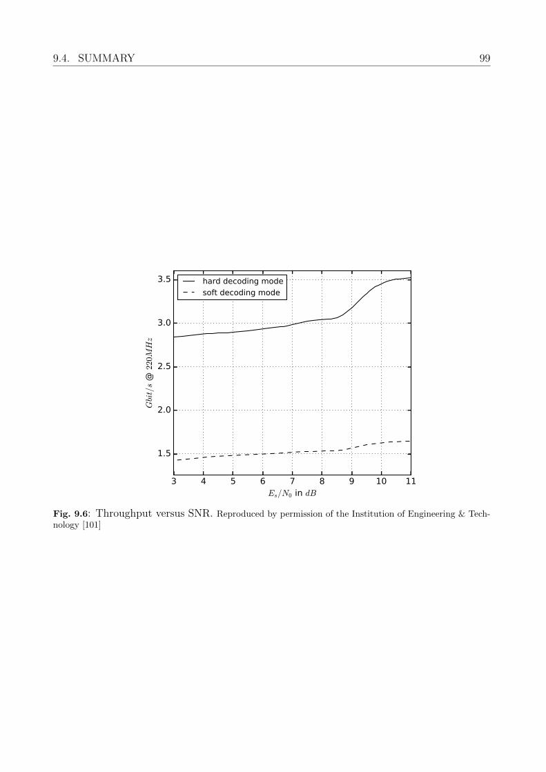
9.4. SUMMARY 99
3 4 5 6 7 8 9 10 11
Es/N0 in dB
1.5
2.0
2.5
3.0
3.5
Gbit/s
@ 220MHz
hard decoding mode
soft decoding mode
i
Fig. 9.6: Throughput versus SNR. Reproduced by permission of the Institution of Engineering & Tech-nology [101]
100
Chapter 10
Conclusion
Flash memories are important non-volatile storage media that have many applications fromconsumer products to industrial storage solutions. However, flash memories require errorcorrection methods to guarantee data reliability. This thesis has investigated error correctiontechniques suitable for flash memories focusing on applications that require very low residualerror rates, e.g. word error rates below 10−16.
The advent of flash memories that provide reliability information about the cell statusled to the introduction of LDPC codes and soft-input decoding for flash memories. How-ever, guaranteeing word error rates as low as 10−16 with LDPC codes is extremely difficultor infeasible. In this thesis, we have proposed a different approach that is based on gener-alized concatenated codes. These codes enable low complexity decoding methods, soft-inputdecoding, and an analysis of the error correction performance for arbitrary low residual errorprobabilities.
We have explained the GC code construction and have developed an approach to determinesuitable code parameters. A major result of this work is a detailed description of the decodingscheme of GC codes. We have presented a complete design for the ECC unit in a flashmemory controller for industrial applications. The decoder achieves a high throughput in thecase where only hard decoding is performed. If a decoding failure occurs, the received wordcan be decoded by a soft-decoder unit in a second pass.
Today’s flash controllers must support different code types, e.g. the decoding of long BCHcodes is required to support older flash technologies. Future research could exploit potentialsynergistic effects of the algebraic decoders for BCH and GC codes. BCH and GC codes usesimilar algorithms. Multipliers, adders, and registers can be shared between the BCH decoderand the outer RS component decoders of the GC code. To quantify these effects furtherinvestigations on such a reconfigurable hardware are necessary.
The results of this thesis led into two patents [US20170331498A1, US20170331499A1].Furthermore, Hyperstone GmbH decided to implement the GCC as an additional ECC intheir micro controller product X1.
101
Bibliography
[1] Solid-State Drive (SSD) Requirements and Endurance Test Method (JESD218). JEDECSOLID STATE TECHNOLOGY ASSOCIATION, 2010.
[2] L.E. Aguado and P.G. Farrell. On hybrid stack decoding algorithms for block codes.Information Theory, IEEE Transactions on, 44(1):398–409, Jan 1998.
[3] Rohit P Ambekar, David B Bogy, Qing Dai, and Bruno Marchon. Critical clearance andlubricant instability at the head-disk interface of a disk drive. Applied Physics Letters,92(3):033104, 2008.
[4] R. E. Blahut. Theory and Practice of Error Control Codes. Addison-Wesley, 1983.
[5] M. Blaum, J. Bruck, and A. Vardy. Interleaving schemes for multidimensional clustererrors. IEEE Transactions on Information Theory, 44(2):730–743, 1998.
[6] Martin Bossert. Channel coding for telecommunications. Wiley, 1999.
[7] Y. Cai, S. Ghose, E. F. Haratsch, Y. Luo, and O. Mutlu. Error characterization, miti-gation, and recovery in flash-memory-based solid-state drives. Proceedings of the IEEE,105(9):1666–1704, Sept 2017.
[8] Y. Cai, E. F. Haratsch, O. Mutlu, and K. Mai. Threshold voltage distribution in MLCNAND flash memory: Characterization, analysis, and modeling. In 2013 Design, Au-tomation Test in Europe Conference Exhibition (DATE), pages 1285–1290, March 2013.
[9] Hsie-Chia Chang and C.B. Shung. New serial architecture for the Berlekamp-Masseyalgorithm. IEEE Transactions on Communications, 47(4):481–483, April 1999.
[10] Hsie-Chia Chang and C.B. Shung. New serial architecture for the Berlekamp-Masseyalgorithm. IEEE Transactions on Communications, pages 481– 483, April 1999.
[11] D Chase. Class of algorithms for decoding block codes with channel measurement infor-mation. IEEE Transactions on Information Theory, pages 170–182, 1972.
[12] R. T. Chien. Cyclic decoding procedure for the Bose-Chaudhuri-Hocquenghem codes. InIEEE Trans. Inform. Theory, 1964.
[13] S. Cho, Daesung Kim, Jinho Choi, and Jeongseok Ha. Block-wise concatenated BCHcodes for NAND flash memories. IEEE Transactions on Communications, 62(4):1164–1177, April 2014.
[14] C. De Almeida and Jr. Palazzo, R. Efficient two-dimensional interleaving technique byuse of the set partitioning concept. Electronics Letters, 32(6):538–540, 1996.
102 BIBLIOGRAPHY
[15] D Divsalar and JH Yuen. Performance of concatenated reed-solomon/viterbi channelcoding. In The Telecommunications and Data Acquisition Report, 1982.
[16] L. Dolecek and Y. Cassuto. Channel coding for nonvolatile memory technologies: Theo-retical advances and practical considerations. Proceedings of the IEEE, 105(9):1705–1724,Sept 2017.
[17] Guiqiang Dong, Ningde Xie, and Tong Zhang. On the use of soft-decision error-correctioncodes in NAND Flash memory. IEEE Transactions on Circuits and Systems I: RegularPapers, 58(2):429–439, Feb 2011.
[18] Wolfram Drescher. Schaltungsanordnung zur Galoisfeld-Arithmetik. Dissertation TU-Dresden, 2005.
[19] I. Dumer. Concatenated codes and their multilevel generalizations. in Handbook of CodingTheory, Vol. II, Elsevier, Amsterdam, 1998.
[20] A. Fahrner, H. Griesser, R. Klarer, and V.V. Zyablov. Low-complexity GEL codes fordigital magnetic storage systems. IEEE Transactions on Magnetics, 40(4):3093–3095,July 2004.
[21] Achim Fahrner. On Signal Processing and Coding for Digital Magnetic Storage Systems.VDI-Verlag, 2005.
[22] G David Forney. Concatenated codes, 1966.
[23] J. Freudenberger, F. Ghaboussi, and S. Shavgulidze. New coding techniques for codesover Gaussian integers. IEEE Transactions on Communications, 61(8):3114–3124, Aug2013.
[24] J. Freudenberger, F. Ghaboussi, and S. Shavgulidze. Set partitioning and multilevelcoding for codes over Gaussian integer rings. In 9th International ITG Conference onSystems, Communications and Coding (SCC), Munich, pages 1–5, Jan 2013.
[25] J. Freudenberger, M. Rajab, and S. Shavgulidze. Estimation of channel state informationfor non-volatile flash memories. In IEEE 7th International Conference on ConsumerElectronics (ICCE), Sept 2017.
[26] R. Gabrys, F. Sala, and L. Dolecek. Coding for unreliable flash memory cells. IEEECommunications Letters, 18(9):1491–1494, Sept 2014.
[27] R. Gabrys, E. Yaakobi, and L. Dolecek. Graded bit-error-correcting codes with appli-cations to flash memory. IEEE Transactions on Information Theory, 59(4):2315–2327,April 2013.
[28] S. Gerardin, M. Bagatin, A. Paccagnella, K. Grurmann, F. Gliem, T. R. Oldham, F. Irom,and D. N. Nguyen. Radiation effects in flash memories. IEEE Transactions on NuclearScience, 60(3):1953–1969, June 2013.
[29] S.W. Golomb, R. Mena, and Wen-Qing Xu. Optimal interleaving schemes for two-dimensional arrays. IEEE Transactions on Information Theory, 52(9):4223–4229, 2006.

BIBLIOGRAPHY 103
[30] J. Guo, W. Wen, J. Hu, D. Wang, H. Li, and Y. Chen. Flexlevel nand flash storagesystem design to reduce ldpc latency. IEEE Transactions on Computer-Aided Design ofIntegrated Circuits and Systems, 36(7):1167–1180, July 2017.
[31] D. h. Lee and W. Sung. Estimation of nand flash memory threshold voltage distributionfor optimum soft-decision error correction. IEEE Transactions on Signal Processing,61(2):440–449, Jan 2013.
[32] K. Haymaker and C. A. Kelley. Structured bit-interleaved LDPC codes for MLC flashmemory. IEEE Journal on Selected Areas in Communications, 32(5):870–879, May 2014.
[33] K Huber. Codes over Gaussian integers. IEEE Transactions on Information Theory,pages 207–216, 1994.
[34] A. Huebner, J. Freudenberger, R. Jordan, and M. Bossert. Irregular turbo codes andunequal error protection. In Proceedings. 2001 IEEE International Symposium on Infor-mation Theory (IEEE Cat. No.01CH37252), pages 142–, 2001.
[35] Yuan Jiang. A practical guide to error-control coding using Matlab. Artech House, 2010.
[36] D. Kim and J. Ha. Quasi-primitive block-wise concatenated bch codes with collaborativedecoding for nand flash memories. IEEE Transactions on Communications, 63(10):3482–3496, Oct 2015.
[37] D. Kim and J. Ha. Serial quasi-primitive bc-bch codes for nand flash memories. In 2016IEEE International Conference on Communications (ICC), pages 1–6, May 2016.
[38] S. Korkotsides, G. Bikas, E. Eftaxiadis, and T. Antonakopoulos. BER analysis of MLCNAND flash memories based on an asymmetric pam model. In 2014 6th InternationalSymposium on Communications, Control and Signal Processing (ISCCSP), pages 558–561, May 2014.
[39] Hanho Lee. A high-speed low-complexity Reed-Solomon decoder for optical communi-cations. IEEE Transactions on Circuits and Systems II: Express Briefs, 52(8):461–465,2005.
[40] H. Li. Modeling of threshold voltage distribution in NAND flash memory: A monte carlomethod. IEEE Transactions on Electron Devices, 63(9):3527–3532, Sept 2016.
[41] S. Li and T. Zhang. Improving multi-level NAND flash memory storage reliability usingconcatenated BCH-TCM coding. IEEE Transactions on Very Large Scale Integration(VLSI) Systems, 18(10):1412–1420, Oct 2010.
[42] Shu Lin and Daniel J. Costello. Error Control Coding. Upper Saddle River, NJ: Prentice-Hall, 2004.
[43] Wei Lin, Shao-Wei Yen, Yu-Cheng Hsu, Yu-Hsiang Lin, Li-Chun Liang, Tien-ChingWang, Pei-Yu Shih, Kuo-Hsin Lai, Kuo-Yi Cheng, and Chun-Yen Chang. A low powerand ultra high reliability LDPC error correction engine with digital signal processing forembedded nand flash controller in 40nm coms. In Symposium on VLSI Circuits Digestof Technical Papers, pages 1–2, June 2014.
104 BIBLIOGRAPHY
[44] Wei Liu, Junrye Rho, and Wonyong Sung. Low-power high-throughput BCH error cor-rection VLSI design for multi-level cell NAND flash memories. In IEEE Workshop onSignal Processing Systems Design and Implementation (SIPS), pages 303 –308, oct. 2006.
[45] Florence Jessie MacWilliams and Neil James Alexander Sloane. The theory of error-correcting codes. North Holland Publishing Co., June 1988.
[46] Alan B. Marchant. Optical recording: a technical overview. Addison-Wesley, Reading,Mass. [u.a.], 1990.
[47] C. Martinez, R. Beivide, and E. Gabidulin. Perfect codes for metrics induced by circulantgraphs. IEEE Transactions on Information Theory, 53(9):3042–3052, 2007.
[48] J Massey. Shift-register synthesis and BCH decoding. IEEE Transactions on InformationTheory, 1969.
[49] J. Massey. Variable-length codes and the Fano metric. IEEE Transactions on InformationTheory, 18(1):196–198, 1972.
[50] Erwin R. Meinders. Optical data storage: phase-change media and recording, volume 4.Springer, Dordrecht, 2006.
[51] R. Micheloni, A. Marelli, and R. Ravasio. Error Correction Codes for Non-Volatile Mem-ories. Springer, 2008.
[52] Rino Micheloni and Luca Crippa. Solid-State-Drives (SSDs) Modeling. Springer, 2017.
[53] V Yasuyuki Goto V Norikazu Nakamura, V Akiyo Mizutani, and V Hiroshi Chiba V KeijiWatanabe. Head disk interface technologies for high recording density and reliability.Fujitsu Sci. Tech. J, 42(1):113–121, 2006.
[54] A. Neubauer, J. Freudenberger, and V. Kuhn. Coding Theory: Algorithms, Architecturesand Applications. John Wiley & Sons, 2007.
[55] J. Oh, J. Ha, J. Moon, and G. Ungerboeck. Rs-enhanced TCM for multilevel flashmemories. IEEE Transactions on Communications, 61(5):1674–1683, May 2013.
[56] ONFI. Open nand flash interface specification revision 3.0. ONFI Workgroup, PublishedMar, 15:288, 2011.
[57] Jeong-In Park, Kihoon Lee, Chang-Seok Choi, and Hanho Lee. High-speed low-complexityReed-Solomon decoder using pipelined Berlekamp-Massey algorithm and its folded archi-tecture. Journal of semiconductor technology and science, 10(3):193–202, 2010.
[58] V. Pavlushkov, R. Johannesson, and V. V. Zyablov. Unequal error protection for convo-lutional codes. IEEE Transactions on Information Theory, 52(2):700–708, Feb 2006.
[59] S. Plass, A. Dammann, G. Richter, and M. Bossert. Channel correlation properties inOFDM by using time-varying cyclic delay diversity. Journal on Communications, 3(3):19–26, 2008.
[60] Antonios Prodromakis, Stelios Korkotsides, and Theodore Antonakopoulos. MLC NANDflash memory: Aging effect and chip/channel emulation. Microprocessors and Microsys-tems, 39(8):1052 – 1062, 2015.
BIBLIOGRAPHY 105
[61] A. Rjabov. Hardware-based systems for partial sorting of streaming data. In 2016 15thBiennial Baltic Electronics Conference (BEC), pages 59–62, Oct 2016.
[62] V. Sorokine and F.R. Kschischang. A sequential decoder for linear block codes with avariable bias-term met ric. IEEE Transactions on Information Theory, 44(1):410–416,1998.
[63] Alessandro S. Spinelli, Christian Monzio Compagnoni, and Andrea L. Lacaita. Reliabilityof NAND flash memories: Planar cells and emerging issues in 3D devices. Computers,6(2), 2017.
[64] F. Sun, S. Devarajan, K. Rose, and T. Zhang. Design of on-chip error correction systemsfor multilevel NOR and NAND flash memories. IET Circuits, Devices Systems, 1(3):241–249, June 2007.
[65] B. Tepekule, U. Yavuz, and A.E. Pusane. On the use of modern coding techniques inQR applications. In 21st Signal Processing and Communications Applications Conference(SIU), pages 1–4, 2013.
[66] Chenxu Wang, Yuhong Gao, Liang Han, and Jinxiang Wang. The design of parallelizedBCH codec. 3rd International Congress on Image and Signal Processing (CISP), 2010.
[67] H. Wang, T. Y. Chen, and R. D. Wesel. Histogram-based flash channel estimation. InIEEE International Conference on Communications (ICC), pages 283–288, June 2015.
[68] Jiadong Wang, K. Vakilinia, Tsung-Yi Chen, T. Courtade, Guiqiang Dong, Tong Zhang,H. Shankar, and R. Wesel. Enhanced precision through multiple reads for ldpc decodingin flash memories. IEEE Journal on Selected Areas in Communications, 32(5):880–891,May 2014.
[69] L. Weiburn and J.K. Cavers. Improved performance of Reed-Solomon decoding with theuse of pilot signals for erasure generation. In Vehicular Technology Conference, 1998.VTC 98. 48th IEEE, volume 3, pages 1930–1934 vol.3, May 1998.
[70] J. Wolf. Efficient maximum likelihood decoding of linear block codes using a trellis. IEEETransactions on Information Theory, 24(1):76–80, January 1978.
[71] C. J. Wu, H. T. Lue, T. H. Hsu, C. C. Hsieh, W. C. Chen, P. Y. Du, C. J. Chiu, andC. Y. Lu. Device characteristics of single-gate vertical channel (SGVC) 3D NAND flasharchitecture. In IEEE 8th International Memory Workshop (IMW), pages 1–4, May 2016.
[72] Yingquan Wu. New scalable decoder architectures for Reed-Solomon codes. IEEE Trans-actions on Communications, 63(8):2741–2761, 2015.
[73] E. Yaakobi, L. Grupp, P.H. Siegel, S. Swanson, and J.K. Wolf. Characterization and error-correcting codes for TLC flash memories. In International Conference on Computing,Networking and Communications (ICNC), pages 486–491, Jan 2012.
[74] E. Yaakobi, Jing Ma, L. Grupp, P.H. Siegel, S. Swanson, and J.K Wolf. Error character-ization and coding schemes for flash memories. In IEEE GLOBECOM Workshops, pages1856–1860, December 2010.
106 BIBLIOGRAPHY
[75] C. Yang, Y. Emre, and C. Chakrabarti. Product code schemes for error correction inMLC NAND flash memories. IEEE Transactions on Very Large Scale Integration (VLSI)Systems, 20(12):2302–2314, Dec 2012.
[76] Xinmiao Zhang and K K Parhi. High-speed architectures for parallel long BCH encoders.IEEE Transactions on Very Large Scale Integration (VLSI) Systems, 13(7):872–877, 2005.
[77] Kai Zhao, Wenzhe Zhao, Hongbin Sun, Xiaodong Zhang, Nanning Zheng, and TongZhang. LDPC-in-SSD: Making advanced error correction codes work effectively in solidstate drives. In Presented as part of the 11th USENIX Conference on File and StorageTechnologies (FAST 13), pages 243–256, San Jose, CA, 2013. USENIX.
[78] I. Zhilin and A. Kreschuk. Generalized concatenated code constructions with low over-head for optical channels and nand-flash memory. In 2016 XV International SymposiumProblems of Redundancy in Information and Control Systems (REDUNDANCY), pages177–180, Sept 2016.
[79] L. Zuolo, C. Zambelli, A. Marelli, R. Micheloni, and P. Olivo. LDPC soft decodingwith improved performance in 1x-2x MLC and TLC NAND flash-based solid state drives.IEEE Transactions on Emerging Topics in Computing, PP(99):1–1, 2017.
[80] Victor Zyablov, Sergo Shavgulidze, and Martin Bossert. An introduction to generalizedconcatenated codes. European Transactions on Telecommunications, 10(6):609–622, 1999.
107
Publications of the author
[81] J. Freudenberger, U. Kaiser, and J. Spinner. Concatenated code constructions for er-ror correction in non-volatile memories. In Int. Symposium on Signals, Systems, andElectronics (ISSSE), Potsdam, pages 1–6, Oct 2012.
[82] J. Freudenberger and J. Spinner. Mixed serial/parallel hardware implementation of theBerlekamp-Massey algorithm for BCH decoding in flash controller applications. In Int.Symposium on Signals, Systems, and Electronics (ISSSE), Potsdam, pages 1–5, Oct 2012.
[83] J. Freudenberger and J. Spinner. A configurable Bose-Chaudhuri-Hocquenghem codec ar-chitecture for flash controller applications. Journal of Circuits, Systems, and Computers,23(2):1–15, Feb 2014.
[84] J. Freudenberger, J. Spinner, and S. Shavgulidze. Generalized concatenated codes for cor-recting two-dimensional clusters of errors and independent errors. In Int. Conference onCommunication and Signal Processing (CSP), Castelldefels-Barcelona, pages 1–5, Febru-ary 2014.
[85] J. Freudenberger, J. Spinner, and S. Shavgulidze. Set partitioning of Gaussian integerconstellations and its application to two-dimensional interleaver design. In Int. Confer-ence on Communication and Signal Processing (CSP), Castelldefels-Barcelona, pages 1–5,February 2014.
[86] J. Freudenberger, J. Spinner, and S. Shavgulidze. Set partitioning of Gaussian integerconstellations and its application to two-dimensional interleaving. IET Communications,8(8):1336–1346, May 2014.
[87] J. Freudenberger, T. Wegmann, and J. Spinner. An efficient hardware implementation ofsequential stack decoding of binary block codes. In IEEE 5th International Conferenceon Consumer Electronics - Berlin (ICCE-Berlin), pages 135–138, Sept 2015.
[88] J. Spinner and J. Freudenberger. Hardware-Entwurf einer flexiblen Fehlerkorrekturein-heit fur Flashspeicher. In MPC-Workshop, Aalen, pages 33–40, Jul 2012.
[89] J. Spinner and J. Freudenberger. Generierung von Code-Komponenten fur BCH En-codierer. In MPC-Workshop, Offenburg, pages 43–46, Feb 2012.
[90] J. Spinner and J. Freudenberger. Semi-automatic source code generation for the hardware-implementation of a parallelizable and configurable error correction unit. In 8th Confer-ence on Ph.D. Research in Microelectronics and Electronics (PRIME), Aachen, pages1–4, Jun 2012.
108 PUBLICATIONS OF THE AUTHOR
[91] J. Spinner and J. Freudenberger. Design and implementation of a pipelined decoder forgeneralized concatenated codes. In Proceedings of 27th Symposium on Integrated Circuitsand Systems Design (SBCCI), Aracaju, Brazil, pages 1–16, Sept 2014.
[92] J. Spinner and J. Freudenberger. Decoder architecture for generalized concatenated codes.IET Circuits, Devices & Systems, 9(5):328–335, 2015.
[93] J. Spinner and J. Freudenberger. Soft input decoding of generalized concatenated codesusing a stack decoding algorithm. In Proceedings of 2nd BW-CAR Symposium on Infor-mation and Communication Systems (SInCom), pages 1–5, Dec 2015.
[94] J. Spinner and J. Freudenberger. A decoder with soft decoding capability for high-rate generalized concatenated codes with applications in non-volatile flash memories. InProceedings of 30th Symposium on Integrated Circuits and Systems Design (SBCCI),Fortaleza, Brazil, Sept. 2017.
[95] J. Spinner, J. Freudenberger, C. Baumhof, A. Mehnert, and R. Willems. A BCH decodingarchitecture with mixed parallelization degrees for flash controller applications. In IEEE26th International SOC Conference (SOCC), Erlangen, pages 116–121, Sept 2013.
[96] J. Spinner, J. Freudenberger, and S. Shavgulidze. Sequential decoding of binary blockcodes based on supercode trellises. In 1st BW-CAR Symposium on Information andCommunication Systems (SInCom), pages 25–28, Nov 2014.
[97] J. Spinner, J. Freudenberger, and S. Shavgulidze. A soft input decoding algorithm forgeneralized concatenated codes. IEEE Transactions on Communications, 64(9):3585–3595, Sept 2016.
[98] J. Spinner, M. Rajab, and J. Freudenberger. Construction of high-rate generalized con-catenated codes for applications in non-volatile flash memories. In 2016 IEEE 8th Inter-national Memory Workshop (IMW), pages 1–4, May 2016.
[99] J. Spinner and J. Freudenberger. Eine effiziente Dekoderarchitektur fur verallgemeinertverkettete Codes. 52. MPC-Workshop, Kunzelsau, pages 27–31, Jul 2014.
[100] J. Spinner and J. Freudenberger. Datenrettung fur die Speicherkarte – Fehlerkorrek-turverfahren fur Flash-Speicher. horizonte, 45:18–20, 2015.
[101] J. Spinner, D. Rohweder, and J. Freudenberger. Soft input decoder for high-rate gener-alised concatenated codes. IET Circuits, Devices & Systems, 2018.
Patents
• US20170331498A1, J. Freudenberger, C. Baumhof, and J. Spinner, Method and devicefor error correction coding based on high-rate generalized concatenated codes, 2017
• US20170331499A1, J. Freudenberger, J. Spinner, and C. Baumhof, Method and decoderfor soft input decoding of generalized concatenated codes, 2017