chapter 24 - transmission lines - qrz.ru · chapter 24 transmission lines t basic theory of...

Transmission Lines 24-1

Chapter 24

Transmission Lines

TBasic Theory of Transmission Lines

he desirability of installing an antenna in a clear space, not too near buildings or power andtelephone lines, cannot be stressed too strongly. On the other hand, the transmitter that generatesthe RF power for driving the antenna is usually, as a matter of necessity, located some distance

from the antenna terminals. The connecting link between the two is the RF transmission line, feeder orfeed line. Its sole purpose is to carry RF power from one place to another, and to do it as efficiently aspossible. That is, the ratio of the power transferred by the line to the power lost in it should be as largeas the circumstances permit.

At radio frequencies, every conductor that has appreciable length compared with the wavelength inuse radiates powerevery conductor is an antenna. Special care must be used, therefore, to minimizeradiation from the conductors used in RF transmission lines. Without such care, the power radiated bythe line may be much larger than that which is lost in the resistance of conductors and dielectrics(insulating materials). Power loss in resistance is inescapable, at least to a degree, but loss by radiationis largely avoidable.

Radiation loss from transmission lines can be prevented by using two conductors arranged andoperated so the electromagnetic field from one is balanced everywhere by an equal and opposite fieldfrom the other. In such a case, the resultant field is zero everywhere in spacethere is no radiationfrom the line.

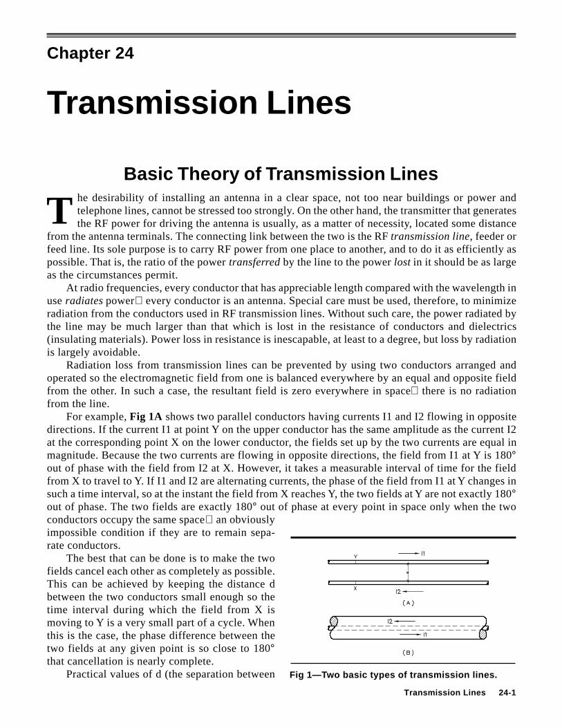
For example, Fig 1A shows two parallel conductors having currents I1 and I2 flowing in oppositedirections. If the current I1 at point Y on the upper conductor has the same amplitude as the current I2at the corresponding point X on the lower conductor, the fields set up by the two currents are equal inmagnitude. Because the two currents are flowing in opposite directions, the field from I1 at Y is 180°out of phase with the field from I2 at X. However, it takes a measurable interval of time for the fieldfrom X to travel to Y. If I1 and I2 are alternating currents, the phase of the field from I1 at Y changes insuch a time interval, so at the instant the field from X reaches Y, the two fields at Y are not exactly 180°out of phase. The two fields are exactly 180° out of phase at every point in space only when the twoconductors occupy the same spacean obviouslyimpossible condition if they are to remain sepa-rate conductors.

The best that can be done is to make the twofields cancel each other as completely as possible.This can be achieved by keeping the distance dbetween the two conductors small enough so thetime interval during which the field from X ismoving to Y is a very small part of a cycle. Whenthis is the case, the phase difference between thetwo fields at any given point is so close to 180°that cancellation is nearly complete.

Practical values of d (the separation betweenFig 1—Two basic types of transmission lines.

24-2 Chapter 24

the two conductors) are determined by the physical limitations of line construction. A separation thatmeets the condition of being “very small” at one frequency may be quite large at another. For example,if d is 6 inches, the phase difference between the two fields at Y is only a fraction of a degree if thefrequency is 3.5 MHz. This is because a distance of 6 inches is such a small fraction of a wavelength(1 λ = 281 feet) at 3.5 MHz. But at 144 MHz, the phase difference is 26°, and at 420 MHz, it is 77°. Inneither of these cases could the two fields be considered to “cancel” each other. Conductor separationmust be very small in comparison with the wavelength used; it should never exceed 1% of the wave-length, and smaller separations are desirable. Transmission lines consisting of two parallel conductorsas in Fig 1A are called open-wire lines, parallel-conductor lines or two-wire lines.

A second general type of line construction is shown in Fig 1B. In this case, one of the conductors istube-shaped and encloses the other conductor. This is called a coaxial line (“coax,” pronounced “co-ax”) orconcentric line. The current flowing on the inner conductor is balanced by an equalcurrent flowing in the opposite direction on the inside surface of the outer conductor. Because of skin effect,the current on the inner surface of the outer conductor does not penetrate far enough to appear on the outsidesurface. In fact, the total electromagnetic field outside the coaxial line (as a result of currents flowing on theconductors inside) is always zero, because the outer conductor acts as a shield at radio frequencies. Theseparation between the inner conductor and the outerconductor is therefore unimportant from the stand-point of reducing radiation.

A third general type of transmission line isthe waveguide. Waveguides are discussed in de-tail in Chapter 18.

CURRENT FLOW IN LONG LINESIn Fig 2, imagine that the connection between

the battery and the two wires is made instantaneouslyand then broken. During the time the wires are incontact with the battery terminals, electrons in wire1 will be attracted to the positive battery terminaland an equal number of electrons in wire 2 will berepelled from the negative terminal. This happensonly near the battery terminals at first, because elec-tromagnetic waves do not travel at infinite speed.Some time does elapse before the currents flow atthe more extreme parts of the wires. By ordinary stan-dards, the elapsed time is very short. Because thespeed of wave travel along the wires may approachthe speed of light at 300,000,000 meters per second,it becomes necessary to measure time in millionthsof a second (microseconds).

For example, suppose that the contact with thebattery is so short that it can be measured in a verysmall fraction of a microsecond. Then the “pulse”of current that flows at the battery terminalsduring this time can be represented by the verticalline in Fig 3. At the speed of light this pulse trav-els 30 meters along the line in 0.1 microsecond,60 meters in 0.2 microsecond, 90 meters in 0.3microsecond, and so on, as far as the line reaches.

The current does not exist all along the wires;it is only present at the point that the pulse has

Fig 2—A representation of current flow on a longtransmission line.

Fig 3—A current pulse traveling along atransmission line at the speed of light wouldreach the successive positions shown atintervals of 0.1 microsecond.


Fig 4—Instantaneous current along atransmission line at successive time intervals.The frequency is 10 MHz; the time for eachcomplete cycle is 0.1 microsecond.

reached in its travel. At this point it is present inboth wires, with the electrons moving in one di-rection in one wire and in the other direction inthe other wire. If the line is infinitely long and hasno resistance (or other cause of energy loss), thepulse will travel undiminished forever.

By extending the example of Fig 3, it is not hardto see that if, instead of one pulse, a whole series ofthem were started on the line at equal time intervals,the pulses would travel along the line with the sametime and distance spacing between them, each pulseindependent of the others. In fact, each pulse couldeven have a different amplitude if the battery voltagewere varied between pulses. Furthermore, the pulsescould be so closely spaced that they touched eachother, in which case current would be present every-where along the line simultaneously.

It follows from this that an alternating voltageapplied to the line would give rise to the sort of cur-rent flow shown in Fig 4. If the frequency of the acvoltage is 10,000,000 Hertz or 10 MHz, each cycleoccupies 0.1 µsecond, so a complete cycle of cur-rent will be present along each 30 meters of line.This is a distance of one wavelength. Any currentsat points B and D on the two conductors occur onecycle later in time than the currents at A and C. Putanother way, the currents initiated at A and C do notappear at B and D, one wavelength away, until theapplied voltage has gone through a complete cycle.

Because the applied voltage is always changing,the currents at A and C change in proportion. The cur-rent a short distance away from A and C—for instance,at X and Y—is not the same as the current at A and C.This is because the current at X and Y was caused bya value of voltage that occurred slightly earlier in thecycle. This situation holds true all along the line; atany instant the current anywhere along the line fromA to B and C to D is different from the current at any other point on that section of the line.

The remaining series of drawings in Fig 4 shows how the instantaneous currents might be distrib-uted if we could take snapshots of them at intervals of 1/4 cycle. The current travels out from the inputend of the line in waves. At any given point on the line, the current goes through its complete range ofac values in one cycle, just as it does at the input end. Therefore (if there are no losses) an ammeterinserted in either conductor reads exactly the same current at any point along the line, because theammeter averages the current over a whole cycle. (The phases of the currents at any two separatepoints is different, but the ammeter cannot show phase.)

VELOCITY OF PROPAGATIONIn the example above it was assumed that energy travels along the line at the velocity of light. The

actual velocity is very close to that of light only in lines in which the insulation between conductors isair. The presence of dielectrics other than air reduces the velocity.

Current flows at the speed of light in any medium only in a vacuum, although the speed in air is

24-4 Chapter 24

close to that in a vacuum. Therefore, the time required for a signal of a given frequency to travel downa length of practical transmission line is longer than the time required for the same signal to travel thesame distance in free space. Because of this propagation delay, 360º of a given wave exists in a physi-cally shorter distance on a given transmission line than in free space. The exact delay for a giventransmission line is a function of the properties of the line, mainly the dielectric constant of the insulat-ing material between the conductors. This delay is expressed in terms of the speed of light (either as apercentage or a decimal fraction), and is referred to as velocity factor (VF). The velocity factor isrelated to the dielectric constant (ε) by

VF = 1ε

(Eq 1)

The wavelength in a practical line is always shorter than the wavelength in free space, which has adielectric constant ε = 1.0. Whenever reference is made to a line as being a “half wavelength” or“quarter wavelength” long (λ/2 or λ/4), it is understood that what is meant by this is the electricallength of the line. The physical length corresponding to an electrical wavelength on a given line isgiven by

λ(feet) = 983.6f VF× (Eq 2)

wheref = frequency in MHzVF = velocity factor

Values of VF for several common types of lines are given later in this chapter. The actual VF of agiven cable varies slightly from one production run or manufacturer to another, even though the cablesmay have exactly the same specifications.

As we shall see later, a quarter-wavelength line is frequently used as an impedance transformer,and so it is convenient to calculate the length of a quarter-wave line directly by

λ/4 245.9f VF= × (Eq 2A)

CHARACTERISTIC IMPEDANCEIf the line could be “perfect”—having no resistive losses—a question might arise: What is the

amplitude of the current in a pulse applied to this line? Will a larger voltage result in a larger current, oris the current theoretically infinite for an applied voltage, as we would expect from applying Ohm’sLaw to a circuit without resistance? The answer is that the current does depend directly on the voltage,just as though resistance were present.

The reason for this is that the current flowing in the line is something like the charging current thatflows when a battery is connected to a capacitor. That is, the line has capacitance. However, it also hasinductance. Both of these are “distributed” properties. We may think of the line as being composed of awhole series of small inductors and capacitors, connected as in Fig 5, where each coil is the inductance of anextremely small section of wire, and the capacitanceis that existing between the same two sections. Eachseries inductor acts to limit the rate at which currentcan charge the following shunt capacitor, and in sodoing establishes a very important property of atransmission line: its surge impedance, more com-monly known as its characteristic impedance. Thisis abbreviated by convention as Z0.

TERMINATED LINESThe value of the characteristic impedance is

equal to L/C in a perfect linethat is, one in

Fig 5—Equivalent of an ideal (lossless) transmissionline in terms of ordinary circuit elements (lumpedconstants). The values of inductance andcapacitance depend on the line construction.


Fig 6—A transmission line terminated in aresistive load equal to the characteristicimpedance of the line.

which the conductors have no resistance and there is no leakage between them—where L and C are theinductance and capacitance, respectively, per unit length of line. The inductance decreases with in-creasing conductor diameter, and the capacitance decreases with increasing spacing between the con-ductors. Hence a line with closely spaced large conductors has a relatively low characteristic imped-ance, while one with widely spaced thin conductors has a high impedance. Practical values of Z0 forparallel-conductor lines range from about 200 to 800 Ω. Typical coaxial lines have characteristic im-pedances from 30 to 100 Ω. Physical constraints on practical wire diameters and spacings limit Z0values to these ranges.

In the earlier discussion of current traveling along a transmission line, we assumed that the line wasinfinitely long. Practical lines have a definite length, and they are terminated in a load at the “output” end(the end to which the power is delivered). In Fig 6, if the load is a pure resistance of a value equal to thecharacteristic impedance of a perfect, lossless line, the current traveling along the line to the load finds thatthe load simply “looks like” more transmission line of the same characteristic impedance.

The reason for this can be more easily understood by considering it from another viewpoint. Along atransmission line, power is transferred successively from one elementary section in Fig 5 to the next. Whenthe line is infinitely long, this power transfer goes on in one directionaway from the source of power.

From the standpoint of section B, Fig 5, for instance, the power transferred to section C has simplydisappeared in C. As far as section B is concerned, it makes no difference whether C has absorbed thepower itself or has transferred it along to more transmission line. Consequently, if we substitute a loadfor section C that has the same electrical characteristics as the transmission line, section B will transferpower into it just as if it were more transmission line. A pure resistance equal to the characteristicimpedance of C, which is also the characteristicimpedance of the line, meets this condition. It ab-sorbs all the power just as the infinitely long lineabsorbs all the power transferred by section B.

Matched LinesA line terminated in a load equal to the com-

plex characteristic line impedance is said to bematched. In a matched transmission line, power istransferred outward along the line from the sourceuntil it reaches the load, where it is completelyabsorbed. Thus with either the infinitely long lineor its matched counterpart, the impedance pre-sented to the source of power (the line-input im-pedance) is the same regardless of the line length.It is simply equal to the characteristic impedanceof the line. The current in such a line is equal tothe applied voltage divided by the characteristicimpedance, and the power put into it is E2/Z0 orI2Z0, by Ohm’s Law.

Mismatched LinesNow take the case where the terminating load

is not equal to Z0, as in Fig 7. The load no longer“looks like” more line to the section of line imme-diately adjacent. Such a line is said to be mis-matched. The more that the load impedance dif-fers from Z0, the greater the mismatch. The powerreaching the load is not totally absorbed, as it waswhen the load was equal to Z0, because the load

Fig 7—Mismatched lines; extreme cases . At A,termination not equal to Z 0; at B, short-circuitedline ; At C, open-circuited line.

24-6 Chapter 24

requires a voltage to current ratio that is different from the one traveling along the line. The result isthat the load absorbs only part of the power reaching it (the incident power); the remainder acts asthough it had bounced off a wall and starts back along the line toward the source. This is known asreflected power, and the greater the mismatch, the larger is the percentage of the incident power that isreflected. In the extreme case where the load is zero (a short circuit) or infinity (an open circuit), all ofthe power reaching the end of the line is reflected back toward the source.

Whenever there is a mismatch, power is transferred in both directions along the line. The voltageto current ratio is the same for the reflected power as for the incident power, because this ratio isdetermined by the Z0 of the line. The voltage and current travel along the line in both directions in thesame wave motion shown in Fig 4. If the source of power is an ac generator, the incident (outgoing)voltage and the reflected (returning) voltage are simultaneously present all along the line. The actualvoltage at any point along the line is the vector sum of the two components, taking into account thephases of each component. The same is true of the current.

The effect of the incident and reflected components on the behavior of the line can be understoodmore readily by considering first the two limiting cases—the short-circuited line and the open-cir-cuited line. If the line is short-circuited as in Fig 7B, the voltage at the end must be zero. Thus theincident voltage must disappear suddenly at the short. It can do this only if the reflected voltage is

opposite in phase and of the same amplitude. Thisis shown by the vectors in Fig 8. The current, how-ever, does not disappear in the short circuit; infact, the incident current flows through the shortand there is in addition the reflected componentin phase with it and of the same amplitude.

The reflected voltage and current must havethe same amplitudes as the incident voltage andcurrent, because no power is dissipated in the shortcircuit; all the power starts back toward the source.Reversing the phase of either the current or volt-age (but not both) reverses the direction of powerflow. In the short-circuited case the phase of thevoltage is reversed on reflection, but the phase ofthe current is not.

If the line is open-circuited (Fig 7C) the cur-rent must be zero at the end of the line. In thiscase the reflected current is 180° out of phase withthe incident current and has the same amplitude.By reasoning similar to that used in the short-cir-cuited case, the reflected voltage must be in phasewith the incident voltage, and must have the sameamplitude. Vectors for the open-circuited case areshown in Fig 9.

Where there is a finite value of resistance (or acombination of resistance and reactance) at the endof the line, as in Fig 7A, only part of the power reach-ing the end of the line is reflected. That is, the re-flected voltage and current are smaller than the inci-dent voltage and current. If R is less than Z0, thereflected and incident voltage are 180° out of phase,just as in the case of the short-circuited line, but theamplitudes are not equal because all of the voltage

Fig 8—Voltage and current at the short circuit on ashort-circuited line. These vectors show how theoutgoing voltage and current (A) combine with thereflected voltage and current (B) to result in highcurrent and very low voltage in the short circuit (C).

Fig 9—Voltage and current at the end of an open-circuited line . At A, outgoing voltage and current;At B, reflected voltage and current ; At C, resultant.


does not disappear at R. Similarly, if R is greater thanZ0, the reflected and incident currents are 180° outof phase (as they were in the open-circuited line),but all of the current does not appear in R. The am-plitudes of the two components are therefore notequal. These two cases are shown in Fig 10. Notethat the resultant current and voltage are in phase inR, because R is a pure resistance.

Nonresistive TerminationsIn most of the preceding discussions, we con-

sidered loads containing only resistance. Further-more, our transmission line was considered to belossless. Such a resistive load will consume some, ifnot all, of the power that has been transferred alongthe line. However, a nonresistive load such as a purereactance can also terminate a length of line. Suchterminations, of course, will consume no power, butwill reflect all of the energy arriving at the end of theline. In this case the theoretical SWR in the line willbe infinite, but in practice, losses in the line will limitthe SWR to some finite value at line positions backtoward the source.

At first you might think there is little or no pointin terminating a line with a nonresistive load. In alater section we shall examine this in more detail, but the value of input impedance depends on the value ofthe load impedance, on the length of the line, the losses in a practical line, and on the characteristic imped-ance of the line. There are times when a line terminated in a nonresistive load can be used to advantage, suchas in phasing or matching applications. Remote switching of reactive terminations on sections of line can beused to reverse the beam heading of an antenna array, for example. The point of this brief discussion is thata line need not always be terminated in a load that will consume power.

Losses in Practical Transmission LinesATTENUATION

Every practical line will have some inherent loss, partly because of the resistance of the conduc-tors, partly because power is consumed in the dielectric used for insulating the conductors, and partlybecause in many cases a small amount of power escapes from the line by radiation. We shall considerhere in detail the losses associated with conductor and dielectric losses.

Matched-Line LossesPower lost in a transmission line is not directly proportional to the line length, but varies logarith-

mically with the length. That is, if 10% of the input power is lost in a section of line of certain length,10% of the remaining power will be lost in the next section of the same length, and so on. For thisreason it is customary to express line losses in terms of decibels per unit length, since the decibel is alogarithmic unit. Calculations are very simple because the total loss in a line is found by multiplyingthe decibel loss per unit length by the total length of the line.

The power lost in a matched line (that is, where the load is equal to the characteristic impedance ofthe line) is called matched-line loss. Matched-line loss is usually expressed in decibels per 100 feet. Itis necessary to specify the frequency for which the loss applies, because the loss does vary with frequency.

Conductor and dielectric loss both increase as the operating frequency is increased, but not in the

Fig 10—Incident and reflected components ofvoltage and current when the line is terminatedin a pure resistance not equal to Z 0. In the caseshown, the reflected components have half theamplitude of the incident components. At A, Rless than Z 0; at B, R greater than Z 0.

24-8 Chapter 24

same way. This, together with the fact that the relative amount of each type of loss depends on theactual construction of the line, makes it impossible to give a specific relationship between loss andfrequency that will apply to all types of lines. Each line must be considered individually. Actual lossvalues for practical lines are given in a later section of this chapter.

One effect of matched-line loss in a real transmission line is that the characteristic impedance, Z0,becomes complex, with a non-zero reactive component X0. Thus,

Z0 = R0 – j X0 (Eq 3)

X –R 0 0= αβ (Eq 4)

where

α = Attenuation (dB/100 feet) 0.1151 (nepers/dB)

100 feet×

,

the attenuation constant, in nepers per unit length

β πλ

= 2

, the phase constant in radians/unit length.

The reactive portion of the complex characteristic impedance is always capacitive (that is, its signis negative) and the value of X0 is usually small compared to the resistive portion R0.

REFLECTION COEFFICIENTThe ratio of the reflected voltage at a given point on a transmission line to the incident voltage is

called the voltage reflection coefficient. The voltage reflection coefficient is also equal to the ratio ofthe incident and reflected currents. Thus

ρ = EE =

II

r

f

r

f (Eq 5)

whereρ = reflection coefficientEr = reflected voltageEf = forward (incident) voltageIr = reflected currentIf = forward (incident) current

The reflection coefficient is determined by the relationship between the line Z0 and the actual loadat the terminated end of the line. In most cases, the actual load is not entirely resistive—that is, the loadis a complex impedance, consisting of a resistance in series with a reactance, as is the complex charac-teristic impedance of the transmission line.

The reflection coefficient is thus a complex quantity, having both amplitude and phase, and isgenerally designated by the Greek letter ρ (rho), or sometimes in the professional literature as Γ (Gamma).The relationship between Ra (the load resistance), Xa (the load reactance), Z0 (the complex line charac-teristic impedance, whose real part is R0 and whose reactive part is X0) and the complex reflectioncoefficient ρ is

ρ = + =±( ) ( )±( ) + ±( )

Z – ZZ Z

R X – R X

R X R Xa 0

a 0

a a 0 0

a a 0 0

* j j

j j

m (Eq 6)

Note that the sign for the X0 term in the numerator of Eq 6 is inverted from that for the denomina-tor, meaning that the complex conjugate of Z0 is actually used in the numerator.

For high-quality, low-loss transmission lines at low frequencies, the characteristic impedance Z0 is


almost completely resistive, meaning that Z0 ≅ R0 and X0 ≅ 0. The magnitude of the complex reflectioncoefficient in Eq 6 then simplifies to:

ρ =( ) +

( ) +

R – R X

R + R X

a 0

2a2

a 0

2a2 (Eq 7)

For example, if the characteristic impedance of a coaxial line at a low operating frequency is 50 Ωand the load impedance is 140 Ω in series with a capacitive reactance of –190 Ω, the magnitude of thereflection coefficient is

ρ = ( ) + ( )+( ) + ( )

=50 –140 –190

50 140 –1900.782

2 2

2 2

Note that the vertical bars on each side of ρ mean the magnitude of rho. If Ra in Eq 7 is equal to R0 and ifXa is 0, the reflection coefficient, ρ, also is 0. This represents a matched condition, where all the energy in theincident wave is transferred to the load. On the other hand, if Ra is 0, meaning that the load has no real resistivepart, the reflection coefficient is 1.0, regardless of the value of R0. This means that all the forward power isreflected, since the load is completely reactive. As we shall see later on, the concept of reflection coefficient isa very useful one to evaluate the impedance seen looking into the input of a mismatched transmission line.

STANDING WAVESAs might be expected, reflection cannot occur at the load without some effect on the voltages and

currents all along the line. To keep things simple for a while longer, let us continue to consider onlyresistive loads, without any reactance. The conclusions we shall reach are valid for transmission linesterminated in complex impedances as well.

The effects are most simply shown by vector diagrams. Fig 11 is an example where the terminatingresistance R is less than Z0. The voltage and current vectors at R are shown in the reference position;they correspond with the vectors in Fig 10A, turned90°. Back along the line from R toward the powersource, the incident vectors, E1 and I1, lead thevectors at the load according to their position alongthe line measured in electrical degrees. (The cor-responding distances in fractions of a wavelengthare also shown.) The vectors representing reflectedvoltage and current, E2 and I2, successively lagthe same vectors at the load.

This lag is the natural consequence of the di-rection in which the incident and reflected com-ponents are traveling, together with the fact that ittakes time for power to be transferred along theline. The resultant voltage E and current I at eachof these positions are shown as dotted arrows. Al-though the incident and reflected componentsmaintain their respective amplitudes (the reflectedcomponent is shown at half the incident-compo-nent amplitude in this drawing), their phase rela-tionships vary with position along the line. Thephase shifts cause both the amplitude and phaseof the resultants to vary with position on the line.

Fig 11—Incident and reflected components atvarious positions along the transmission line,together with resultant voltages and currents atthe same positions. The case shown is for R lessthan Z 0.

24-10 Chapter 24

If the amplitude variations (disregarding phase) of the resultant voltage and current are plottedagainst position along the line, graphs like those of Fig 12A will result. If we could go along the linewith a voltmeter and ammeter measuring the current and voltage at each point, plotting the collecteddata would give curves like these. In contrast, if the load matched the Z0 of the line, similar measure-ments along the line would show that the voltage is the same everywhere (and similarly for the cur-rent). The mismatch between load and line is responsible for the variations in amplitude which, be-cause of their stationary, wave-like appearance, are called standing waves.

Some general conclusions can be drawn from inspection of the standing-wave curves: At a position180° (λ/2) from the load, the voltage and current have the same values they do at the load. At a position 90°from the load, the voltage and current are “inverted.” That is, if the voltage is lowest and current highest atthe load (when R is less than Z0), then 90° from the load the voltage reaches its highest value. The currentreaches its lowest value at the same point. In the casewhere R is greater than Z0, so the voltage is highestand the current lowest at the load, the voltage is low-est and the current is highest 90° from the load.

Note that the conditions at the 90° point alsoexist at the 270° point (3λ/4). If the graph werecontinued on toward the source of power it wouldbe found that this duplication occurs at every pointthat is an odd multiple of 90º (odd multiple of λ/4)from the load. Similarly, the voltage and currentare the same at every point that is a multiple of180° (any multiple of λ/2) away from the load.

Standing-Wave RatioThe ratio of the maximum voltage (resulting

from the interaction of incident and reflected volt-ages along the line) to the minimum voltage—thatis, the ratio of Emax to Emin in Fig 12A, is definedas the voltage standing-wave ratio (VSWR) or sim-ply standing-wave ratio (SWR).

SWREE

II

max

min

max

min= = (Eq 8)

The ratio of the maximum current to the mini-mum current is the same as the VSWR, so eithercurrent or voltage can be measured to determinethe standing-wave ratio. The standing-wave ratiois an index of many of the properties of a mis-matched line. It can be measured with fairly simpleequipment, so it is a convenient quantity to use inmaking calculations on line performance.

The SWR is related to the magnitude of the com-plex reflection coefficient by

SWR = 1+1 –

ρρ

(Eq 9)

and conversely the reflection coefficient magnitudemay be defined from a measurement of SWR as

ρ = SWR – 1SWR 1+

(Eq 10)

Fig 12—Standing waves of current and voltagealong the line for R less than Z 0. At A, resultantvoltages and currents along a mismatched lineare shown at B and C. At B, R less than Z 0; At C,R greater than Z 0.


We may also express the reflection coefficient in terms of forward and reflected power, quantities whichcan be easily measured using a directional RF wattmeter. The reflection coefficient may be computed as

ρ = PP

r

f (Eq 11)

wherePr = power in the reflected wavePf = power in the forward wave.From Eq 10, SWR is related to the forward and reflected power by

SWR = 1 + 1 –

= 1 + P /P

1 – P /Pr f

r f

ρρ

(Eq 12)

Fig 13 converts Eq 12 into a convenient nomograph. In the simple case where the load contains noreactance, the SWR is numerically equal to the ratio between the load resistance R and the characteris-tic impedance of the line. When R is greater than Z0,

SWR = RZ0

(Eq 13)

When R is less than Z0,

SWR = ZR

0 (Eq 14)

(The smaller quantity is always used in the denominator of the fraction so the ratio will be a num-ber greater than 1.)

Flat LinesAs discussed earlier, all the power that is transferred along a transmission line is absorbed in the

load if that load is a resistance value equal to the Z0 of the line. In this case, the line is said to beperfectly matched. None of the power is reflected back toward the source. As a result, no standingwaves of current or voltage will be developed along the line. For a line operating in this condition, thewaveforms drawn in Fig 12A become straight lines, representing the voltage and current delivered by

Fig 13—SWR as a function of forward and reflected powe r.

24-12 Chapter 24

the source. The voltage along the line is constant, so the minimum value is the same as the maximumvalue. The voltage standing-wave ratio is therefore 1:1. Because a plot of the voltage standing wave isa straight line, the matched line is also said to be flat.

ADDITIONAL POWER LOSS DUE TO SWRThe power lost in a given line is least when the line is terminated in a resistance equal to its characteristic

impedance, and as stated previously, that is called the matched-line loss. There is however an additional lossthat increases with an increase in the SWR. This is because the effective values of both current and voltagebecome greater on lines with standing waves. The increase in effective current raises the ohmic losses (I2R) inthe conductors, and the increase in effective voltage increases the losses in the dielectric (E2/R).

The increased loss caused by an SWR greater than 1:1 may or may not be serious. If the SWR at the load isnot greater than 2:1, the additional loss caused by the standing waves, as compared with the loss when the line isperfectly matched, does not amount to more than about 1/2 dB, even on very long lines. One-half dB is an unde-tectable change in signal strength. Therefore, it can be said that, from a practical standpoint in the HF bands, anSWR of 2:1 or less is every bit as good as a perfect match, so far as additional losses due to SWR are concerned.

However, above 30 MHz, in the VHF and especially the UHF range, where low receiver noise figuresare essential for effective weak-signal work, matched-line losses for commonly available types of coax canbe relatively high. This means that even a slight mismatch may become a concern regarding overall trans-mission line losses. At UHF one-half dB of additional loss may be considered intolerable!

The total loss in a line, including matched-line and the additional loss due to standing waves may becalculated from Eq 15 below.

Total Loss (dB) = 10 log a –

a 1 –

2 2

2

ρρ( )

(Eq 15)

where

a = 10 ML

10 = matched-line loss ratio

ρ = SWR – 1SWR + 1 = magnitude of reflection coefficient

whereML = the matched-line loss for particular length of line, in dBSWR = SWR at load end of line

Thus, the additional loss caused by the standing waves is calculated from:

Additonal loss (dB) = Total Loss – ML (Eq 16)

For example, RG-213 coax at 14.2 MHz is rated at 0.795 dB of matched-line loss per 100 feet.A 150 foot length of RG-213 would have an overall matched-line loss of

(0.795/100) × 150 = 1.193 dB

Thus, if the SWR at the load end of the RG-213 is 4:1,

α

ρ

= 10 = 1.316

= 4 – 14 + 1 = 0.600

and the total line loss = 10 log1.316 – 0.6001.316 1 – 0.600

= 2.12 dB.

1.193/10

2 2

2( )

The additional loss due to the SWR of 4:1 is 2.12 – 1.19 = 0.93 dB.


LINE VOLTAGES AND CURRENTSIt is often desirable to know the voltages and currents that are developed in a line operating with

standing waves. The voltage maximum may be calculated from Eq 17 below, and the other valuesdetermined from the result.

E P Z SWRmax 0= × × (Eq 17)

whereEmax = voltage maximum along the line in the presence of standing wavesP = power delivered by the source to the line input, wattsZ0 = characteristic impedance of the line, ohmsSWR = SWR at the load

If 100 W of power is applied to a 50 Ω line with an SWR at the load of 10:1, Emax= 100 600 10× × = 774.6 V. Based on Eq 8, Emin, the minimum voltage along the line equalsEmax/SWR = 774.6/10 = 77.5 V. The maximum current may be found by using Ohm’s Law. Imax =Emax/Z0 =774.6/600 = 1.29 A. The minimum current equals Imax/SWR = 1.29/10 = 0.129 A.

The voltage determined from Eq 17 is the RMS value—that is, the voltage that would be measured withan ordinary RF voltmeter. If voltage breakdown is a consideration, the value from Eq 17 should be con-verted to an instantaneous peak voltage. Do this by multiplying times 2 (assuming the RF waveform is asine wave). Thus, the maximum instantaneous peak voltage in the above example is 774.6 × 2 = 1095.4 V.

Strictly speaking, the values obtained as above apply only near the load in the case of lines with appre-ciable losses. However, the resultant values are the maximum possible that can exist along the line, whetherthere are line losses or not. For this reason they are useful in determining whether or not a particular line canoperate safely with a given SWR. Voltage ratings for various cable types are given in a later section.

Fig 14 shows the ratio of current or voltage at a loop, in the presence of standing waves, to the current orvoltage that would exist with the same power in a perfectly matched line. As with Eq 17 and related calcula-tions, the curve literally applies only near the load.

Input ImpedanceThe effects of incident and reflected voltage and

current along a mismatched transmission line canbe difficult to envision, particularly when the loadat the end of the transmission line is not purely re-sistive, and when the line is not perfectly lossless.

If we can put aside for a moment all the com-plexities of reflections, SWR and line losses, a trans-mission line can simply be considered to be an im-pedance transformer. A certain value of load im-pedance, consisting of a resistance and reactance,at the end of a particular transmission line is trans-formed into another value of impedance at the in-put of the line. The amount of transformation is de-termined by the electrical length of the line, its char-acteristic impedance, and by the losses inherent inthe line. The input impedance of a real, lossy trans-mission line is computed using the following equa-tion, called the Transmission Line Equation

Z Z

Z cosh Z sinhZ sinh Z coshin 0

L 0

L 0

= × ( ) + ( )( ) + ( )

γ γγ γl l

l l(Eq 18)

Fig 14—Increase in maximum value of current orvoltage on a line with standing waves, as referredto the current or voltage on a perfectly matchedline, for the same power delivered to the load.Voltage and current at minimum points are given bythe reciprocals of the values along the vertical axis.The curve is plotted from the relationship, current(or voltage) ratio = the square root of SWR.

24-14 Chapter 24

Fig 15—Input impedance of a line terminated in aresistance. This impedance can be representedby either a resistance and reactance in series, ora resistance and reactance in parallel, at a singlefrequenc y. The relationships between the R and Xvalues in the series and parallel equivalents aregiven by the equations shown. X may be eitherinductive or capacitive, depending on the linelength, Z 0 and the load impedance, which neednot be purely resistive.

whereZin= complex impedance at input of lineZL = complex load impedance at end of line = Ra ± j XaZ0 = characteristic impedance of line = R0 ± j X0l = physical length of lineγ = complex loss coefficient = α + j βα = matched-line loss attenuation constant, in nepers/unit length (1 neper = 8.688 dB; cables are

rated in dB/100 ft)β = phase constant of line in radians/unit length (related to physical length of line l by the fact that

2π radians = one wavelength, and by Eq 2)

= × 2

VF 983.6/f (MHz), for in feetπ l

VF = velocity factorl = electrical length of line in same units of length measurement (feet) as α or β aboveFor example, assume that a halfwave dipole terminates a 50-foot long piece of RG-213 coax. This

dipole is assumed to have an impedance of 43 + j 30 Ω at 7.15 MHz, and its velocity factor is 0.66. Thematched-line loss at 7.15 MHz is 0.27 dB and the characteristic impedance Z0 for this type of cable is50 − j 0.44 Ω. Using Eq 18, we compute the impedance at the input of the line as 65.8 + j 32.1 Ω.

Solving this equation manually is quite tedious, but it may be solved using a traditional paper SmithChart or a computer program. Chapter 28 details the use of the Smith Chart. ARRL MicroSmith, a sophisti-cated graphical Smith Chart program written for the IBM PC, is available through the ARRL. TLA (Trans-mission Line, Advanced) is another ARRL programthat performs this transformation, but without SmithChart graphics. TLA.EXE is on the diskette accom-panying this edition of The ARRL Antenna Book.

One caution should be noted when using anyof these computational tools to calculate the im-pedance at the input of a mismatched transmis-sion linethe velocity factor of practical trans-mission lines can vary significantly betweenmanufacturing runs of the same type of cable. Forhighest accuracy, you should measure the veloc-ity factor of a particular length of cable beforeusing it to compute the impedance at the end ofthe cable. See Chapter 27 for details on measure-ments of line characteristics.

Series and Parallel Equivalent CircuitsOnce the series-form impedance Rs ± j Xs at

the input of a particular line has been determined,either by measurement or by computation, youmay wish to determine the equivalent parallel cir-cuit, which is equivalent to the series form only ata single frequency. The equivalent parallel circuitis often useful when designing a matching circuit(such as an antenna tuner, for example) to trans-form the impedance at the input of the cable toanother impedance. The following equations areused to make the transformation from series toparallel and from parallel to series. See Fig 15.


RR X

Rps s

s

2 2

= +(Eq 19A)

XR X

Xps s

s

2 2

= + (Eq 19B)

and

RR X

R Xsp p

p p

2

2 2=+ (Eq 20A)

XR X

R Xsp

2p

p p2 2=

+ (Eq 20B)

The individual values in the parallel circuit are not the same as those in the series circuit (although theoverall result is the same, but only at one frequency), but are related to the series-circuit values by theseequations. For example, let us continue the example in the section above, where the impedance at the inputof the 50 feet of RG-213 at 7.15 MHz is 65.8 + j 32.1 Ω. The equivalent parallel circuit at 7.15 MHz is

R65.8 32.1

65.8 81.46

X65.8 32.1

31.2 169.97

p

p

2 2

2 2

= + =

= + =

Ω

Ω

If we were to put 100 W of power into this parallel equivalent circuit, the voltage across the parallelcomponents would beSince

P = ER

2, E = P R 100 81.46 90.26 V× = × =

Thus, the current through the inductive part of the parallel circuit would be

I EX

90.26169.97 0.53 A.

p= = =

Highly Reactive LoadsWhen highly reactive loads are used with practical transmission lines, especially coax lines, the overall

loss can reach staggering levels. For example, a popular multiband antenna is a 100-foot long center-feddipole located some 50 feet over average ground. At 1.83 MHz, such an antenna will exhibit a feed-pointimpedance of 4.5 − j 1673 Ω, according to the mainframe analysis program NEC2. The high value of capaci-tive reactance indicates that the antenna is extremely short electrically after all, a halfwave dipole at 1.83MHz is almost 270 feet long, compared to this 100-foot long antenna. If an amateur attempts to feed such amultiband antenna directly with 100 feet of RG-213 50-Ω coaxial cable, the SWR at the antenna terminalswould be (using the TLA program) 1828:1. An SWR of more than 1800 to 1 is a very high level of SWRindeed! At 1.83 MHz the matched-line loss of 100 feet of the RG-213 coax by itself is only 0.24 dB. How-ever, the total line loss due to this extreme level of SWR is 26 dB.

This means that if 100 W is fed into the input of this line, the amount of power at the antenna isreduced to only 0.25 W! Admittedly, this is an extreme case. It is more likely that an amateur wouldfeed such a multiband antenna with open-wire “ladder” or “window” line than coaxial cable. The matched-line loss characteristics for 450-Ω “window” open-wire line are far better than coax, but the SWR at theend of this line is still 397:1, resulting in an overall loss of 12.1 dB. Even for low-loss open-wire line,the total loss is significant because of the extreme SWR.

24-16 Chapter 24

This means that only about 6% of the power from the transmitter is getting to the antenna, andalthough this is not very desirable, it is a lot better than the losses in coax cable feeding the sameantenna! However, at a transmitter power level of 1500 W, the maximum voltage at an antenna tunerused to match this line impedance is almost 7600 V with the open-wire line, a level which will certainlycause arcing or burning inside! (As a small compensation for all the loss in coax under this extremecondition, so much power is lost that the voltages present in the antenna tuner are not excessive.) Keepin mind also that an antenna tuner can lose significant power in internal losses for very high impedancelevels, even if it has sufficient range to match such impedances in the first place.

Clearly, it would be far better to use a longer antenna at this 160-meter frequency. Another alterna-tive would be to resonate a short antenna with loading coils (at the antenna). Either strategy would helpavoid excessive feed line loss, even with low-loss line.

SPECIAL CASESBeside the primary purpose of transporting power from one point to another, transmission lines

have properties that are useful in a variety of ways. One such special case is a line an exact multiple ofλ/4 (90°) long. As shown earlier, such a line will have a purely resistive input impedance when thetermination is a pure resistance. Also, short-circuited or open-circuited lines can be used in place ofconventional inductors and capacitors since such lines have an input impedance that is substantially apure reactance when the line losses are low.

The Half- Wavelength LineWhen the line length is an even multiple of 90° (that is, a multiple of λ/2), the input resistance is equal to

the load resistance, regardless of the line Z0. As a matter of fact, a line an exact multiple ofλ/2 in length (disregarding line losses) simply repeats, at its input or sending end, whatever impedance existsat its output or receiving end. It does not matter whether the impedance at the receiving end is resistive,reactive, or a combination of both. Sections of line having such length can be added or removed withoutchanging any of the operating conditions, at least when the losses in the line itself are negligible.

Impedance Transformation with Quarter- Wave LinesThe input impedance of a line an odd multiple of λ/2 long is

ZZZi

02

L= (Eq 21)

where Zi is the input impedance and ZL is the load impedance. If ZL is a pure resistance, Zi will also bea pure resistance. Rearranging this equation gives

Z Z Z0 i L= (Eq 22)

This means that if we have two values of impedance that we wish to “match,” we can do so if weconnect them together by a λ/4 transmission line having a characteristic impedance equal to the squareroot of their product.

A λ/4 line is, in effect, a transformer, and in fact is often referred to as a quarter-wave transformer.It is frequently used as such in antenna work when it is desired, for example, to transform the imped-ance of an antenna to a new value that will match a given transmission line. This subject is consideredin greater detail in a later chapter.

Lines as Circuit ElementsTwo types of nonresistive line terminations are quite usefulæshort and open circuits. The imped-

ance of the short-circuit termination is 0 + j 0, and the impedance of the open-circuit termination isinfinite. Such terminations are used in stub matching. (See Chapters 26 and 28.) An open or short-circuited line does not deliver any power to a load, and for that reason is not, strictly speaking a “trans-mission” line. However, the fact that a line of the proper length has inductive reactance makes itpossible to substitute the line for a coil in an ordinary circuit. Likewise, another line of appropriate


Fig 16—Lumped-constant circuit equivalents ofopen and short-circuited transmission lines.

length having capacitive reactance can be substi-tuted for a capacitor.

Sections of lines used as circuit elements areusually λ/4 or less long. The desired type of reac-tance (inductive or capacitive) or the desired typeof resonance (series or parallel) is obtained byshorting or opening the far end of the line. Thecircuit equivalents of various types of line sec-tions are shown in Fig 16.

When a line section is used as a reactance, theamount of reactance is determined by the character-istic impedance and the electrical length of the line.The type of reactance exhibited at the input termi-nals of a line of given length depends on whether itis open- or short-circuited at the far end.

The equivalent “lumped” value for any “in-ductor” or “capacitor” may be determined with theaid of the Smith Chart or Eq 18. Line losses maybe taken into account if desired, as explained forEq 18. In the case of a line having no losses, andto a close approximation when the losses are small,the inductive reactance of a short-circuited lineless than λ/4 in length is

XL (ohms) = Z

0 tan l (Eq 23)

where l is the length of the line in electrical degrees and Z0 is the characteristic impedance of the line.The capacitive reactance of an open-circuited line less than l/4 in length is

XC (ohms) = Z

0 cot l (Eq 24)

Lengths of line that are exact multiples of λ/4 have the properties of resonant circuits. With anopen-circuit termination, the input impedance of the line acts like a series-resonant circuit. With ashort-circuit termination, the line input simulates a parallel-resonant circuit. The effective Q of suchlinear resonant circuits is very high if the line losses, both in resistance and by radiation, are keptdown. This can be done without much difficulty, particularly in coaxial lines, if air insulation is usedbetween the conductors. Ai r-insulated open-wire lines are likewise very good at frequencies for whichthe conductor spacing is very small in terms of wavelength.

Applications of line sections as circuit elements in connection with antenna and transmission-linesystems are discussed in later chapters.

Line Construction and Operating CharacteristicsThe two basic types of transmission lines, parallel conductor and coaxial, can be constructed in a

variety of forms. Both types can be divided into two classes, (1) those in which the majority of the insulationbetween the conductors is air, where only the minimum of solid dielectric necessary for mechanical support isused, and (2) those in which the conductors are embedded in and separated by a solid dielectric. Thefirst variety (air insulated) has the lowest loss per unit length, because there is no power loss in dry air if thevoltage between conductors is below the value at which corona forms. At the maximum power permitted inamateur transmitters, it is seldom necessary to consider corona unless the SWR on the line is very high.

AIR-INSULATED LINESA typical construction technique used for parallel conductor or “two wire” air-insulated transmis-

24-18 Chapter 24

Fig 18—Characteristic impedance as a function of con-ductor spacing and size for parallel conductor lines.

sion lines is shown in Fig 17. The two wires are supported a fixed distance apart by means of insulatingrods called spacers. Spacers may be made from material such as Teflon, Plexiglas, phenolic, polysty-rene, plastic clothespins or plastic hair curlers. Materials commonly used in high quality spacers areisolantite, Lucite and polystyrene. (Teflon is generally not used because of its higher cost.) The spacerlength varies from 2 to 6 inches. The smaller spacings are desirable at the higher frequencies (28 MHz)so radiation from the transmission line is minimized.

Spacers must be used at small enough intervals along the line to keep the two wires from movingappreciably with respect to each other. For amateur purposes, lines using this construction ordinarilyhave #12 or #14 conductors, and the characteristic impedance is between 500 to 600 Ω. Although onceused nearly exclusively, such homemade lines are enjoying a renaissance of sorts because of their highefficiency and low cost.

Where an air insulated line with still lower characteristic impedance is needed, metal tubing from1/4 to 1/2-inch diameter is frequently used. With thelarger conductor diameter and relatively closespacing, it is possible to build a line having acharacteristic impedance as low as about 200 Ω.This construction technique is principally used forλ/4 matching transformers at the higher frequencies.

The characteristic impedance of an air-insu-lated parallel conductor line, neglecting the effectof the spacers, is given by

Z0 276= log 2Sd

(Eq 25)

whereZ

0 = characteristic impedance in ohms

S = center-to-center distance between conductorsd = outer diameter of conductor (in the same

units as S)Impedances for common sizes of conductors

over a range of spacings are given in Fig 18.

Four-Wire LinesAnother parallel conductor line that is useful in

some applications is the four-wire line(Fig 19C). In cross section, the conductors of thefour-wire line are at the corners of a square. Spac-ings are on the same order as those used in two-wirelines. The conductors at opposite corners of thesquare are connected to operate in parallel. This typeof line has a lower characteristic impedance than thesimple two-wire type. Also, because of the more sym-metrical construction, it has better electrical balanceto ground and other objects that are close to the line.The spacers for a four-wire line may be discs of in-sulating material, X-shaped members, etc.

Air-Insulated Coaxial LinesIn air-insulated coaxial lines (Fig 19D), a con-

siderable proportion of the insulation between con-ductors may actually be a solid dielectric, because

Fig 17—Typical open-wire line construction. Thespacers may be held in place by beads of solder orepoxy cement. Wire wraps can also be used, as shown.


the separation between the inner and outer conductors must be constant. This is particularly likely to be truein small diameter lines. The inner conductor, usually a solid copper wire, is supported at the center of thecopper tubing outer conductor by insulating beads or a helically wound strip of insulating material. Thebeads usually are isolantite, and the wire is gener-ally crimped on each side of each bead to preventthe beads from sliding. The material of which thebeads are made, and the number of beads per unitlength of line, will affect the characteristic imped-ance of the line. The greater the number of beads ina given length, the lower the characteristic imped-ance compared with the value obtained with air in-sulation only. Teflon is ordinarily used as a helicallywound support for the center conductor. A tighterhelical winding lowers the characteristic impedance.

The presence of the solid dielectric also increasesthe losses in the line. On the whole, however, a co-axial line of this type tends to have lower actual loss,at frequencies up to about 100 MHz, than any otherline construction, provided the air inside the line canbe kept dry. This usually means that air- tight sealsmust be used at the ends of the line and at every joint.

The characteristic impedance of an air-insu-lated coaxial line is given by

Z0 138= log Dd

(Eq 26)

whereZ0 = characteristic impedance in ohmsD = inside diameter of outer conductord = outside diameter of inner conductor (in same units as D)Values for typical conductor sizes are graphed

in Fig 20. The equation and the graph for coaxiallines are approximately correct for lines in whichbead spacers are used, provided the beads are nottoo closely spaced.

FLEXIBLE LINESTransmission lines in which the conductors are

separated by a flexible dielectric have a number ofadvantages over the air-insulated type. They are lessbulky, weigh less in comparable types and maintainmore uniform spacing between conductors. They arealso generally easier to install, and are neater in ap-pearance. Both parallel conductor and coaxial linesare available with flexible insulation.

The chief disadvantage of such lines is that thepower loss per unit length is greater than in air-insu-lated lines. Power is lost in heating of the dielectric,and if the heating is great enough (as it may be withhigh power and a high SWR), the line may breakdown mechanically and electrically.

Fig 19—Construction of air-insulatedtransmission lines.

Fig 20—Characteristic impedance of typical air-insulated coaxial lines.

24-20 Chapter 24

Fig 21—Construction of flexible parallelconductor and coaxial lines with solid dielectric.A common variation of the double shieldeddesign at D has the braids in continuouselectrical contact.

Parallel-Conductor LinesThe construction of a number of types of flexible

line is shown in Fig 21. In the most common 300-Ωtype (twin-lead), the conductors are stranded wireequivalent to #20 in cross-sectional area, and aremolded in the edges of a polyethylene ribbon about1/2 inch wide that keeps the wires spaced away a con-stant amount from each other. The effective dielectricis partly solid and partly air, and the presence of thesolid dielectric lowers the characteristic impedanceof the line as compared with the same conductors inair. The resulting impedance is approximately 300 Ω.

Because part of the field between the conduc-tors exists outside the solid dielectric, dirt andmoisture on the surface of the ribbon tend tochange the characteristic impedance of the line.The operation of the line is therefore affected byweather conditions. The effect will not be veryserious in a line terminated in its characteristicimpedance, but if there is a considerable mismatch,a small change in Z0 may cause wide fluctuationsof the input impedance. Weather effects can beminimized by cleaning the line occasionally andgiving it a thin coating of a water repellent mate-rial such as silicone grease or car wax.

To overcome the effects of weather on the char-acteristic impedance and attenuation of ribbon typeline, another type of twin-lead is made using an ovalpolyethylene tube with an air core or a foamed di-electric core. The conductors are molded diametri-cally opposite each other in the walls. This increasesthe leakage path across the dielectric surface. Also,much of the electric field between the conductors isin the hollow (or foam-filled) center of the tube. Thistype of line is fairly impervious to weather effects.Care should be used when installing it, however, soany moisture that condenses on the inside withchanges in temperature and humidity can drain outat the bottom end of the tube and not be trapped inone section. This type of line is made in two con-ductor sizes (with different tube diameters), one forreceiving applications and the other for transmitting.

Transmitting type 75-Ω twin-lead uses strandedconductors nearly equivalent to solid #12 wire, withquite close spacing between conductors. Because ofthe close spacing, most of the field is confined to thesolid dielectric, with very little existing in the sur-rounding air. This makes the 75-Ω line much less sus-ceptible to weather effects than the 300-Ω ribbon type.

A third type of commercial parallel-line is so-called window line, illustrated in Fig 21C. This is avariation of twin-lead construction, except that “win-


dows” are cut in the polyethylene insulation at regular intervals. This holds down on the weight of the line,and also breaks up the amount of surface area where dirt, dust and moisture can accumulate. Such “window”line is commonly available with a nominal characteristic impedance of 450 Ω, although 300-Ω line can befound also. A conductor spacing of about 1 inch is used in the 450-Ω line and 1/2 inch in the 300-Ω line. Theconductor size is usually about #18. The impedances of such lines are somewhat lower than given by Fig 18for the same conductor size and spacing, because of the effect of the dielectric constant of the spacer materialused. The attenuation is quite low and lines of this type are entirely satisfactory for transmitting applicationsat amateur power levels.

COAXIAL CABLESCoaxial cable is available in flexible and semiflexible varieties. The fundamental design is the

same in all types, as shown in Fig 21. The outer diameter varies from 0.06 inch to over 5 inches. Power-handling capability and cable size are directly proportional, as larger dielectric thickness and largerconductor sizes can handle higher voltages and currents. Generally, losses decrease as cable diameterincreases. The extent to which this is true is dependent on the properties of the insulating material.

Some coaxial cables have stranded wire center conductors while others use a solid copper conduc-tor. Similarly, the outer conductor (shield) may be a single layer of copper braid, a double layer of braid(more effective shielding), solid aluminum (Hardline), aluminum foil, or a combination of these.

Losses and DeteriorationThe power-handling capability and loss characteristics of coaxial cable depend largely on the dielectric

material between the conductors. The commonly used cables and some of their properties are listed inTable 1. Fig 22 is a graph of the attenuation characteristics versus frequency for the most popular lines. The

Fig 22—Nominal matched-line attenuation in decibels per 100 feet of various common transmission lines.Total attenuation is directly proportional to length . Attenuation will vary somewhat in actual cablesamples, and generally increases with age in coaxial cables having a type I jacket. Cables groupedtogether in the above chart have approximately the same attenuation. Types having foam polyethylenedielectric have slightly lower loss than equivalent solid types, when not specifically shown above.

24-22 Chapter 24

Table 1Characteristics of Commonly Used Transmission Lines

pF Max. RMSZ0 VF per OD Dielectric Operating

Type of line Ω % foot inches Material Volts(Belden No.)RG-6 (1152A) 75.0 75 16.5 0.266 Foam PE 300RG-8X (9258) 50.0 78 26.0 0.242 Foam PE 300RG-8 (8237) 52.0 66 29.5 0.405 PE 3700RG-8 (8214) 50.0 78 26.0 0.405 Foam PE 600RG-8A (9251) 52.0 66 29.5 0.405 PE 3700RG-9 (8242) 51.0 66 30.0 0.420 PE 3700RG-9A 51.0 66 30.0 0.420 PE 3700RG-9B 50.0 66 30.8 0.420 PE 3700RG-11 (8238) 75.0 66 20.5 0.405 PE 3700RG-11 (8213) 75.0 78 17.4 0.405 Foam PE 600RG-11A (8261) 75.0 66 20.5 0.405 PE 3700RG-12 75.0 66 20.6 0.475 PE 3700RG-12A 75.0 66 20.6 0.475 PE 3700RG-17 52.0 66 29.5 0.870 PE 11000RG-17A 52.0 66 29.5 0.870 PE 11000RG-55 53.5 66 28.5 0.216 PE 1900RG-55A 50.0 66 30.8 0.216 PE 1900RG-55B 53.5 66 28.5 0.216 PE 1900RG-58 (8240) 53.5 66 28.5 0.195 PE 1400RG-58A (8259) 50.0 66 30.8 0.195 PE 1400RG-58A (8219) 50.0 78 26.0 0.195 Foam PE 300RG-58B 53.5 66 28.5 0.195 PE 1400RG-58C (8262) 50.0 66 30.8 0.195 PE 1400RG-59 (8241) 75.0 66 20.5 0.242 PE 1700RG-59 (8212) 75.0 79 16.9 0.242 Foam PE 300RG-59B (8263) 75.0 66 20.5 0.242 PE 1700RG-62 (8254) 93.0 86 13.5 0.242 Air-spaced PE 750RG-62 foam 95.0 79 13.4 0.242 Foam PE 300RG-62A (9228) 93.0 86 13.5 0.242 Air-spaced PE 750RG-62B (8255) 93.0 86 13.5 0.242 Air-spaced PE 750RG-133A 95.0 66 16.2 0.405 PE 4000RG-141 50.0 70 29.0 0.190 PTFE 1400RG-141A (83241) 50.0 70 29.0 0.190 PTFE 1400RG-142 (84142) 50.0 70 29.0 0.206 PTFE 1400RG-142A 50.0 70 29.0 0.206 PTFE 1400RG-142B (83242) 50.0 70 29.0 0.195 PTFE 1400RG-174 (8216) 50.0 66 30.8 0.100 PE 1100RG-213 (8267) 50.0 66 30.8 0.405 PE 3700RG-214* (8268) 50.0 66 30.8 0.425 PE 3700RG-215 50.0 66 30.8 0.475 PE 3700RG-216 (9850) 75.0 66 20.5 0.425 PE 3700RG-218 (ex RG-17) 52.0 66 29.5 0.870 PE 11000RG-223* (9273) 50.0 66 30.8 0.212 PE 17009913 (Belden)* 50.0 89 24.0 0.405 Air-spaced PE 6009914 (Belden)* 50.0 78 26.0 0.405 Foam PE 600

Aluminum Jacket, Foam Dielectric1/2 inch 50.0 81 25.0 0.500 25003/4 inch 50.0 81 25.0 0.750 40007/8 inch 50.0 81 25.0 0.875 45001/2 inch 75.0 81 16.7 0.500 25003/4 inch 75.0 81 16.7 0.750 35007/8 inch 75.0 81 16.7 0.875 4000

Open wire — 97 — — —75-Ω transmitting twin lead 75.0 67 19.0 — —300-Ω twin lead 300.0 82 5.8 — —300-Ω tubular 300.0 80 4.6 — —

Open Wire Line, “Window” Type (#18 conductors)1/2 inch 300.0 95 — — —1 inch 450.0 95 — — —

Dielectric Name Temperature LimitsDesignationPE Polyethylene –65° to +80° CFoam PE Foamed polyethylene –65° to +80° CPTFE Polytetrafluoroethylene –250° to +250° C

(Teflon)*Double shield


Table 2Coaxial Cable Equations

C (pf/ft) = 7.26

log(D/d)

L ( H/ft) = 0.14 log Dd

Z0 (ohms) = LC

138log

Dd

VF% (velocity factor, ref. speed of light = 100

Time delay (ns/ft) = 1.016

f(cutoff/GHz) = 7.50

(D + d)

Refl coef = = Z

L – Z0

ZL

Z0

= SWR – 1SWR + 1

SWR = 1 +

1 –

Vpeak = (1.15 Sd) (log D/d)

K

A = 0.435Z0D

Dd

ε

µ

ε

ε

ε

ε

ρ

ρρ

=

+

(K1(K1 K2) f + 2.78 (PF)(f)+

ε

whereA = atten in dB/100 ftd = OD of inner conductorD = ID of outer conductorS = max voltage gradient of insulation in

volts/mile = dielectric constantK = safety factorK1 = strand factorK2 = braid factorf = freq in MHzPF = power factor

Note: Obtain K1 and K2 data from manufacturer.

(Eq A)

(Eq B)

(Eq C)

(Eq D)

(Eq E)

(Eq F)

(Eq G)

(Eq H)

(Eq I)

(Eq J)

outer insulating jacket of the cable (usually PVC) isused solely as protection from dirt, moisture andchemicals. It has no electrical function. Exposureof the inner insulating material to moisture andchemicals over time contaminates the dielectric andincreases cable losses. Foam dielectric cables areless prone to contamination than are solid-polyeth-ylene insulated cables.

Impregnated cables, such as Decibel ProductsVB-8 and Times Wire & Cable Co. Imperveon,are immune to water and chemical damage, andmay be buried if desired. They also have a self-healing property that is valuable when rodentschew into the line. Cable loss should be checkedat least every two years if the cable has been out-doors or buried. See the earlier section on testingtransmission lines.

The pertinent characteristics of unmarkedcoaxial cables can be determined from the equationsin Table 2. The most common impedance valuesare 52, 75 and 95 Ω. However, impedances from25 to 125 Ω are available in special types of manu-factured line. The 25-Ω cable (miniature) is used ex-tensively in magnetic-core broadband transformers.

Cable CapacitanceThe capacitance between the conductors of

coaxial cable varies with the impedance and di-electric constant of the line. Therefore, the lowerthe impedance, the higher the capacitance per foot,because the conductor spacing is decreased. Ca-pacitance also increases with dielectric constant.

Voltage and Power RatingsSelection of the correct coaxial cable for a par-

ticular application is not a casual matter. Not only isthe attenuation loss of significance, but breakdownand heating (voltage and power) also need to beconsidered. If a cable were lossless, the power-handling capability would be limited only by the breakdownvoltage. RG-58, for example, can withstand an operating potential of 1400 V RMS. In a 52-Ω system thisequates to more than 37 kW, but the current corresponding to this power level is 27 amperes, which wouldobviously melt the conductors in RG-58. In practical coaxial cables, the copper and dielectric losses, ratherthan breakdown voltage, limit the maximum power that can be accommodated. If 1000 W is applied to acable having a loss of 3 dB, only 500 W is delivered to the load. The remaining 500 W must be dissipated inthe cable. The dielectric and outer jacket are good thermal insulators, which prevent the conductors fromefficiently transferring the heat to free air.

As the operating frequency increases, the power-handling capability of a cable decreases becauseof increasing conductor loss (skin effect) and dielectric loss. RG-58 with foam dielectric has a break-down rating of only 300 V, yet it can handle substantially more power than its ordinary solid dielectriccounterpart because of the lower losses. Normally, the loss is inconsequential (except as it affectspower-handling capability) below 10 MHz in amateur applications. This is true unless extremely long

24-24 Chapter 24

runs of cable are used. In general, full legal amateur power can be safely applied to inexpensive RG-58coax in the bands below 10 MHz. Cables of the RG-8 family can withstand full amateur power throughthe VHF spectrum, but connectors must be carefully chosen in these applications. Connector choice isdiscussed in a later section.

Excessive RF operating voltage in a coaxial cable can cause noise generation, dielectric damageand eventual breakdown between the conductors.

Shielded Parallel LinesShielded balanced lines have several advantages over open-wire lines. Since there is no noise pickup on

long runs, they can be buried and they can be routed through metal buildings or inside metal piping. Shieldedbalanced lines having impedances of 140 or 100 Ω can be constructed from two equal lengths of 70-Ω or 50-Ωcable (RG-59 or RG-58 would be satisfactory for amateur power levels). Paralleled RG-63 (125-Ω) cable wouldmake a balanced transmission line more in accord with traditional 300-Ω twin-lead feed line (Z0 = 250 Ω).

The shields are connected together (see Fig 23A), and the two inner conductors constitute the balancedline. At the input, the coaxial shields should be connected to chassis ground; at the output (the antenna side),

they are joined but left floating.A high power, low-loss, low-impedance 70-Ω

(or 50-Ω) balanced line can be constructed from fourcoaxial cables. See Fig 23B. Again, the shields areall connected together. The center conductors of thetwo sets of coaxial cables that are connected in par-allel provide the balanced feed.

Coaxial FittingsThere is a wide variety of fittings and connec-

tors designed to go with various sizes and types ofsolid-dielectric coaxial line. The “UHF” series offittings is by far the most widely used type in theamateur field, largely because they are widely avail-able and are inexpensive. These fittings, typified bythe PL-259 plug and SO-239 chassis fitting (mili-tary designations) are quite adequate for VHF and

Fig 24—The PL-259 or UHF connector is almost universal for amateur HF work and is popular forequipment operating up through the VHF range. Steps for assembly are given in detail in the text.

Fig 23—Shielded balanced transmission linesutilizing standard small-size coaxial cable, suchas RG-58 or RG-59. These balanced lines may berouted inside metal conduit or near large metalobjects without adverse effects.


Fig 25—Crimp-on connectors and adapters for use with standard PL-259 connectors are popular forconnecting to RG-58 and RG-59 coax. (This material courtesy of Amphenol Electronic Components,RF Division, Bunker Ramo Corp.)

Fig 26—Assembly of the 83 series (SO-239) with hoods. Complete electrical shield integrity in the UHFfemale connector requires that the shield be attached to the connector flange by means of a hood.

lower frequency applications, but are not weatherproof. Neither do they exhibit a 52-Ω impedance.Type N series fittings are designed to maintain constant impedance at cable joints. They are a bit harder to

assemble than the “UHF” type, but are better for frequencies above 300 MHz or so. These fittings are weath-erproof.

The BNC fittings are for small cable such as RG-58, RG-59 and RG-62. They feature a bayonet-

24-26 Chapter 24

Fig 27—BNC connectors are common on VHF and UHF equipment at low power levels. (Courtesy ofAmphenol Electronic Components, RF Division, Bunker Ramo Corp.)

locking arrangement for quick connect and disconnect, and are weatherproof. They exhibit a constantimpedance.

Methods of assembling connectors on the cable are shown in Figs 24 through 28. The most com-mon or longest established connector in each series is illustrated. Several variations of each type exist.Assembly instructions for coaxial fittings not shown here are available from the manufacturers.

PL-259 AssemblyFig 24 shows how to install the solder type of PL-259 connector on RG-8 type cable. Proper prepa-

ration of the cable end is the key to success. Follow these simple steps.

1) Measure back 3/4 inch from the cable end and slightly score the outer jacket around itscircumference.


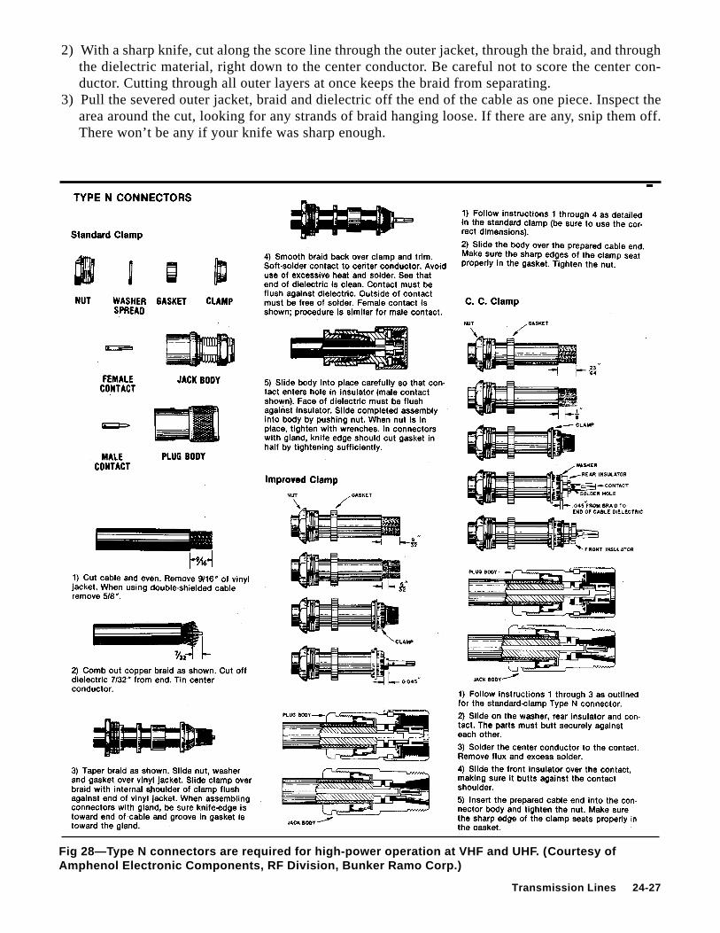
Fig 28—Type N connectors are required for high-power operation at VHF and UHF. (Courtesy ofAmphenol Electronic Components, RF Division, Bunker Ramo Corp.)

2) With a sharp knife, cut along the score line through the outer jacket, through the braid, and throughthe dielectric material, right down to the center conductor. Be careful not to score the center con-ductor. Cutting through all outer layers at once keeps the braid from separating.

3) Pull the severed outer jacket, braid and dielectric off the end of the cable as one piece. Inspect thearea around the cut, looking for any strands of braid hanging loose. If there are any, snip them off.There won’t be any if your knife was sharp enough.

24-28 Chapter 24

4) Next, score the outer jacket 5/16 inch back from the first cut. Cut through the jacket lightly; do notscore the braid. This step takes practice. If you score the braid, start again.

5) Remove the outer jacket. Tin the exposed braid and center conductor, but apply the solder sparingly.Avoid melting the dielectric.

6) Slide the coupling ring onto the cable. (Don’t forget this important step!)7) Screw the connector body onto the cable. If you prepared the cable to the right dimensions, the

center conductor will protrude through the center pin, the braid will show through the solder holes,and the body will actually thread itself onto the outer cable jacket.

8) With a large soldering iron, solder the braid through each of the four solder holes. Use enough heat toflow the solder onto the connector body, but not so much as to melt the dielectric. Poor connection to thebraid is the most common form of PL-259 failure. This connection is just as important as that betweenthe center conductor and the connector. With some practice you’ll learn how much heat to use.

9) Allow the connector body to cool somewhat, and then solder the center connector to the center pin.The solder should flow on the inside, not the outside of the pin. Trim the center conductor to be evenwith the end of the center pin. Use a small file to round the end, removing any solder that may havebuilt up on the outer surface of the center pin. Use a sharp knife, very fine sandpaper, or steel woolto remove any solder flux from the outer surface of the center pin.

10) Screw the coupling onto the body, and the job is finished.

Fig 25 shows two options for using RG-58 or RG-59 cable with PL-259 connectors. The crimp-onconnectors manufactured for the smaller cable work well if installed correctly. The alternative methodinvolves using adapters for the smaller cable with standard PL-259 connectors made for RG-8. Preparethe cable as shown in Fig 24. Once the braid is prepared, screw the adapter into the PL-259 shell andfinish the job as you would with RG-8 cable.

Fig 26 shows how to assemble female SO-239 connectors onto coaxial cable. Figs 27 and 28respectively show the assembly of BNC and type N connectors.

SINGLE WIRE LINEThere is one type of line, in addition to those already described, that deserves mention because it is still

used to a limited extent. This is the single wire line, consisting simply of a single conductor running from thetransmitter to the antenna. The “return” circuit for such a line is the earth; in fact, the second conductor of theline can be considered to be the image of the actual conductor in the same way that an antenna strung abovethe earth has an image (see Chapter 3). The characteristic impedance of the single wire line depends on theconductor size and the height of the wire above ground, ranging from 500 to 600 Ω for #12 or #14 conduc-tors at heights of 10 to 30 feet. The characteristic impedance may be calculated from

Z = 138 log 4hd0 (Eq 27)

whereZ0 = characteristic impedance of the single wire lineh = antenna heightd = wire diameter, in same units as hBy connecting the line to the antenna at a point that represents a resistive impedance of 500 to

600 Ω, the line can be matched and operated without standing waves.Although the single wire line is very simple to install, it has at least two outstanding disadvan-

tages. First, because the return circuit is through the earth, the behavior of the system depends on thekind of ground over which the antenna and transmission lines are erected. In practice, it may not bepossible to get the necessary good connection to actual ground that is required at the transmitter. Sec-ond, the line always radiates, because there is no nearby second conductor to cancel the fields. Radia-tion is minimum when the line is properly terminated, because the line current is lowest under theseconditions. The line is, however, always a part of the radiating antenna system, to some extent.


LINE INSTALL ATION

Installing Coax LineOne great advantage of coaxial line, particularly the flexible dielectric type, is that it can be in-

stalled with almost no regard for its surroundings. It requires no insulation, can be run on or in theground or in piping, can be bent around corners with a reasonable radius, and can be “snaked” throughplaces such as the space between walls where it would be impractical to use other types of lines.However, coaxial lines should always be operated in systems that permit a low SWR, and precautionsmust be taken to prevent RF currents from flowing on the outside of the line. This is discussed inChapter 26. Additional information on line installation is given in Chapter 4.

Installing Parallel-Wire LinesIn installing a parallel-wire line, care must be used to prevent it from being affected by moisture,

snow and ice. In home construction, only spacers that are impervious to moisture and are unaffected bysunlight and weather should be used on air-insulated lines. Steatite spacers meet this requirement ad-equately, although they are somewhat heavy. The wider the line spacing, the longer the leakage pathacross the spacers, but this cannot be carried too far without running into line radiation, particularly atthe higher frequencies. Where an open-wire line must be anchored to a building or other structure,standoff insulators of a height comparable with the line spacing should be used if mounted in a spotthat is open to the weather. Lead-in bushings for bringing the line into a building also should have along leakage path.

The line should be kept away from other conductors, including downspouts, metal window frames,flashing, etc, by a distance of two or three times the line spacing. Conductors that are very close to theline will be coupled to it to some degree, and the effect is that of placing an additional load across theline at the point where the coupling occurs. Reflections take place from this coupled “load,” raising theSWR. The effect is at its worst when one wire is closer than the other to the external conductor. In sucha case one wire carries a heavier load than the other, with the result that the line currents are no longerequal. The line then becomes unbalanced.

Solid dielectric, two-wire lines have a relatively small external field because of the small spacing,and can be mounted within a few inches of other conductors without much danger of coupling betweenthe line and such conductors. Standoff insulators are available for supporting lines of this type whenrun along walls or similar structures.

Sharp bends should be avoided in any type of transmission line, because such bends cause a changein the characteristic impedance. The result is that reflections take place from each bend. This is of lessimportance when the SWR is high than when an attempt is being made to match the load to the line Z0.It may be impossible to get the SWR to the desired figure until bends in the line are made very gradual.

TESTING TRANSMISSION LINESCoaxial cable loss should be checked at least every two years if the cable is installed outdoors or

buried. (See later section on losses and deterioration.) Testing of any type of line can be done using thetechnique illustrated in Fig 29. If the measured loss in watts equates to more than 1 dB over the rated

Fig 29—Method for determining losses intransmission lines. The impedance of thedummy load must equal the Z 0 of the line foraccurate results.

24-30 Chapter 24

loss per 100 feet, the line should be replaced. The matched-line loss in dB can be determined from

dB = l0 log PP

i

2(Eq 28)

wherePi is the power at the transmitter outputP2 is the power measured at RL of Fig 29.Yet other methods of determining line losses may be used. If the line input impedances can be

measured accurately with a short and then an open-circuit termination, the electrical line length (deter-mined by velocity factor) and the matched-line loss may be calculated for the frequency of measure-ment. The procedure is described in Chapter 28.

Determining line characteristics as just mentioned requires the use of a laboratory style of imped-ance bridge, or at least an impedance or noise bridge calibrated to a high degree of accuracy. But usefulinformation about a transmission line can also be learned with just an SWR indicator, if it offersreliable readings at high SWR values.

A lossless line theoretically exhibits an infinite SWR when terminated in an open or a short circuit. Apractical line will have losses, and therefore will limit the SWR at the line input to some finite value.Provided the signal source can operate safely into a severe mismatch, an SWR indicator can be used todetermine the line loss. The instruments available to most amateurs lose accuracy at SWR values greaterthan about 5:1, so this method is useful principally as a go/no-go check on lines that are fairly long. Forshort, low-loss cables, only significant deterioration can be detected by the open-circuit SWR test.

First, either open or short circuit one end of the line. It makes no difference which termination is used,as the terminating SWR is theoretically infinite in either case. Then measure the SWR at the other end of theline. The matched-line loss for the frequency of measurement may then be determined from

Lm = 10 log SWR +1SWR – 1

(Eq 29)

where SWR = the SWR value measured at the line input

BIBLIOGRAPHYSource material and more extended discussion of topics covered in this chapter can be found in the

references given below and in the textbooks listed at the end of Chapter 2.

C. Brainard and K. Smith, “Coaxial Cable—The Neglected Link,” QST, Apr 1981, pp 28-31.D. DeMaw, “In-Line RF Power Metering,” QST, Dec 1969.D. Geiser, “Resistive Impedance Matching with Quarter-Wave Lines,” QST, Feb 1963, pp 56-57.H. Jasik, Antenna Engineering Handbook, 1st ed. (New York: McGraw-Hill, 1961).R. C. Johnson and H. Jasik, Antenna Engineering Handbook, 2nd ed. (New York: McGraw-Hill, 1984),

pp 43-27 to 43-31.R. W. P. King, H. R. Mimno and A. H. Wing, Transmission Lines, Antennas and Waveguides (New

York: Dover Publications, Inc., 1965).J. D. Kraus, Antennas (New York: McGraw-Hill Book Co., 1950).Kurokawa, “Power Waves and the Scattering Matrix,” IEEE Transactions on Microwave Theory and

Techniques, Vol MTT-13, Mar 1965, pp 194-202.M. W. Maxwell, “Another Look at Reflections,” QST, Apr, Jun, Aug and Oct 1973, Apr and Dec 1974,

and Aug 1976.M. W. Maxwell, Reflections (ARRL: Newington, CT, 1990).T. McMullen, “The Line Sampler, an RF Power Monitor for VHF and UHF,” QST, April 1972.H. Weinstein, “RF Transmission Cable for Microwave Applications,” Ham Radio, May 1985, p 106.

chapter 24 - transmission lines - qrz.ru · chapter 24 transmission lines t basic theory of...

Documents