chapter9 sensitivity-calibration decision-support tools ... · sensitivity-calibration...
TRANSCRIPT
Chapter9
Sensitivity-calibration Decision-support Tools for Continuous SWMM Modeling: a Fuzzy-logic Approach
William James aad Alltlloay William Kaelt
Eight software tools and analytical methods are suggested that would render very-long-term, continuous, surface water quality management modeling more productive and more credible. This chapter focuses on the US EPA Storm Water Management Model (SWMM). Two tools are described in detail: (i) a heuristic sensitivity analysis (SA) methodology written as a shell around SWMM4, and (ii) a calibration methodology. The first uses concepts from fuzzy logic and is accomplished by grouping 48 SWMM RUNOFF block parameters by hydrologic processes and identifying the dominant processes in various limited inputparameter spaces by matching combinations of parameters to classes of hydrometeorological events. Both were developed, integrated, and tested using a SWMM datafile for Redhill Creek in Hamilton, Ontario.
9. I Introduction
Arguments for development of a decision support shell (here taken to mean a user interface of integrated software tools) for complex hydrology and hydraulics models are well known (James, 1994a). Traditionally, flood hazard mitigation has been the driving force behind the implementation of storm drainage facilities. Today, engineers are sensitive to, and accountable for, the interaction
James, W. and A. Kuch. 1998. "Sensitivity-calibration Decision-support Tools for Continuous SWMM Modeling: a Fuzzy-logic Approach." Journal of Water Management Modeling R200-09. doi: 10.14796/JWMM.R200-09. ©CHI 1998 www.chijoumal.org ISSN: 2292-6062 (Formerly in Advances in Modeling the Management ofStormwater Impacts. ISBN: 0-9697422-8-2)
159
160 Fuzzy-logic and Sensitivity Calibration/or Continuous SWMM
of their designs with natural systems, i.e. the ecosystem impacts. The need for conceptual and credible modeling has never been greater, as clients and the public no longer accept narrow solutions to stormwater quality and quantity problems. Computer interfaces (shells) which integrate several complex models, information management systems and management of the modeling are also becoming popular under the rubric of decision support systems (DSS, Orlob 1992). Automated and process-oriented sensitivity analysis is a first step towards the development of most of the modeling tools described in this chapter, which is oriented to long-term water quality management modeling.
It is to the modeler's advantage to use the most complex, deterministic, process model available or possible, because new understanding of water quality processes active in a real situation is gained. Systematic dissaggregation of these models helps develop the user's knowledge of the real system. Hence this chapter targets complex urban surface water quality models, which can then be used to evaluate several best management strategies, for a variety of objectives, such as:
1. characterize surface runoff, concentration and load ranges; 2. determine effects, magnitudes, locations, and ~ombinations of
quality and quantity control options; 3. provide input to a receiving water quality analysis, e.g. drive a
receiving water quality model such as WASP5; 4. perform frequency analyses on quality parameters, e.g. determine
return periods of concentrations and loads; and 5. provide input to cost-benefit analyses ofbestmanagementpractices
(BMPs) and control options (Huber, 1992, EI-Hosseiny, 1996). Calibration of a continuous SWMM model can be an arduous task. There
are typically dozens, often hundreds and occasionally thousands of parameters describing many active processes in a typical SWMM RUNOFF simulation. Adjustment of a parameter may result in a closer prediction to one or a group of observations but also result in a poorer estimate of other observations. This occurs because SWMM parameters display different sensitivity for various precipitation and meteorological inputs. The adjustment of a parameter may have a greater effect on the model's response to large storms than to small storms, or long durations as opposed to short durations. A methodology allowing modelers to systematically calibrate parameters by isolating dominant processes helps modelers to generate a reliable continuous model.
In this chapter, a previously calibrated SWMM RUNOFF dataset for Hamilton, Ontario was chosen. First, a heuristic sensitivity analysis on this dataset was performed using the SA tool. The comprehensive SA allows the identification of active processes, sensitive parameters and the generation of sensitivity gradients for use in the calibration process. The parameter sensitivity was plotted using concepts from fuzzy logic, a value of 1.0 for a sensitive parameter, 0.0 for insensitive. Second, the parameter sensitivity and the dominance of the physically-based processes were analyzed and presented graphically
9.2 Background Review 161
in fuzzy terms. Third, a synthetic time series (TS) was prepared by running the as-is calibrated model using a very long-term continuous rainfall record. Fourth, a calibration to the syntheticTS was undertaken by the following two methods:
I. Systematic calibration by groups of parameters for each process using unique events in the time series that isolate the dominance of the processes, the parameters being adjusted in order :from most sensitive to least sensitive.
2. Calibration using PEST software, where the selection of adjustable parameters was guided by a general set of rules derived:from the SA (this method is not presented in this chapter).
In both cases the model was calibrated to the synthetic TS and a measurement of best-fit determined for each. In other words, the model was calibrated to a TS generated by a model with a known parameter set by running the model with a suitable continuous rainfall TS. This exercise eliminates the field noise from the data (these errors have been addressed by others and consideration of them is not an integral part of this study). Both calibrations commenced :from the same corrupted dataset and were compared to the synthetic TS. The rainfall TS used was a 41-yr continuous record :from the Toledo, Ohio Airport in NCDC hourly format.
9.2 Background Review
We suggest that the following tools are required to model stormwater quality with more credibility:
1. long duration six minute interval (more or less) rain TS tools and synthetic generators;
2. statistics presentation tools for three generation (3G, 7 5 years) input and output TS;
3. sensitivity analysis tools for selected SWMM model parameters; 4. calibration tools and techniques; 5. error analysis tools; 6. fuzzy poUutograph/hydrograph output that represents a probability
of the solution; 7. procedures to evaluate the comparative cost-effective performance
of various combinations of better storm water quality management proposals (arrays of best management practices (BMPs)); and
8. a graphical user interface to integrate the above tools and enhance productivity.
Tools 3 and 8 were designed and developed for this study as the sensitivity analysis tool and user interface. For this study we developed a toolbox shell that acts as a graphical user interface (GUI) environment for managing SWMM input and output files. When the user pulls-down this menu the user sees:
162 Fuzzy-logic and Sensitivity Calibration for Continuous SWMM
Sensitivity Analysis - Menu item for the SAT. Synthetic Rainfall TS - Hook for the synthetic rainfall TS tool. CalibrationIV erification - Hook to PEST software. Error Analysis - Hook for the error analysis tool. Fuzzy Hydrograph/
Pollutograph - Hook for the fuzzy output tool 3GM Statistics - Hook for the 3G statistics tool. BMP Cost Analysis - Hook for the BMP cost analysis tool. These seven tools are described conceptually below.
Five/six minute rain time series The primary input function to all surface water quality models such as
SWMM is rainfall time series. The continuous simulation approach is often thwarted because of the need for continuous rainfall data relevant to the catcbment(s) being modeled. The 5 (or 6)-minute rain time series tool should address:
1. programs to generate synthetic TS from coarse, discrete observations or statistical parameters;
2. techniques to manage copious TS and render it usable for SWMM; 3. utilities to access existing databases including CD ROM, electronic
BBSs, and Intemetlweb sources; 4. programs to modify and transpose observed rain data from one
climatic region to another; and 5. software to extract suitable events from a TS for sensitivity testing
and model inference. Information and models are available on the generation of synthetic rainfall
time series, e.g. R. Srikanthanand Tom McMahon (1985). Also, atthe University of Guelph two tools (CASCADE and CASCADE2) were recently developed (Gregory, 1995; and Wang, 1996). These link the SWMM RAIN block with ANNIE, the TS manager for HSP-F and with HEC-DSS, the TS manager for the HEC software suite. On another front, commercial sources provide meteorological time series for thousands of locations in North America, in hourly and 15 minute data of more than 40 years duration in some cases. Within the framework of sensitivity based tools it is appropriate that the rainfall time series be easily divided into events suitable for testing the sensitivity of the model. Dominant model processes are isolated by rainfall events. For example, the rainfall TS tool should be able to extract a storm eventthatmeets a given descriptive criteria such as a maximum of 0.25 hours in duration with a maximum intensity of at least 75 mmIhr. Such a precipitation event is called a short-duration high-intensity event, and excites overland flow on impervious areas causing the PCTZER, IMPDEP and IMPERN parameters to be sensitive. The DSS must have a graphical user interface that allows:
9.2 Background Review
1. scrolling visually through the TS; 2. altering the time and abscissa scale allowing zooming; 3. color coding of the rainfall data based on user criteria such as
intensity; 4. graphical editing of the data into a format for SWMM(E cards); and 5. allowing factors to be applied such as 25.4 to convert inches to mm.
Statistics Presentation
163
To aid in the conceptualization ofthree-generatio modeling (3GM), it is proposed to modify the statistics block ofSWMM, especially as it relates to the comparative 75-year performance and evaluation of alternative combinations of BMPs. This modification should include summaries of the number of total exceedencesldeficits and the duration of exceedencesldeficits of flow rate or constituent concentration. This enables the modeler to better evaluate aquatic habitat and fluviology impacts for very long TS. The time series are analyzed by reading the flows and/or concentrations for a single location on the interface file. The TS is then divided into events based on user-entered criteria. The events are then sorted and the top 50 ranked for any of the following: duration of the event, inter-event duration, peak concentrations or flows, and runoff volume or loads. The following modifications to the STA TS block are needed:
• include a minimum criteria to analyze for deficits such as a critical low flow of a stream;
• count and report the total number of exCeec:lences or deficits; • count and report the duration of exceedences and/or deficits for the
total simulation; and • trend analysis for average loads and flows on an annual basis to be
used in conjunction with modifications to alter the parameters on an annual basis. '
The Statistics Tool also requires a graphical software tool to present the results in tabular and graphical plots of at least two TS for the comparison of an alternative to some benchmark such as a pre-existing condition.
Error Analysis An important and often overlooked aspect of modeling is the understanding.
analysis, prediction, and reporting of errors. Parameters which must be estimated or optimized, if they are sensitive and their values are far from optimum, can be great sources of error. Sensitivity analysis and the resulting parameter sensitivity gradients can be applied to error analysis (EA) in many ways.
Fuzzy Pollutograph and Hydrograph Output Currently, SWMM computes and outputs a single-valued hydrograph o~
pollutograph, which is inappropriate, considering the inherent uncertainty in the modeled processes, noisy field data, and other errors. The computed output
164 Fuzzy-logic and Sensitivity Calibration jor Continuous SWMM
should optionally be presented as a range of values based on probability and error. Model uncertainty is not reflected in the single valued answer, which creates false assurance in the results (Baffaut and Delleur, 1990). Sensitivity gradients can be used to create an upper and lower band that represents the range of the probable solution. The region bounded by these TS could be plotted as the probable range of valid computed response.
Cost-Effective Performance Evaluation Procedures jor BMPs The evaluation of the relative cost-effective performance of many alterna
tive combinations of better management procedures (such as gross pollutant traps, detention ponds, infiltration recharge facilities, real-time-control or intelligent drains) is the goal of this tool.
Sensitivity Analysis Software has been written to automatically perform a heuristic sensitivity
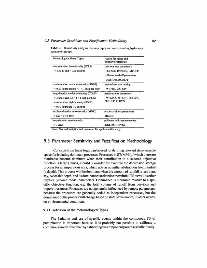
analysis on 48 RUNOFF block parameters. The 48 parameters have been grouped by processes and are separately accessed by the user in different dialogue boxes for each process group by the sensitivity analysis tool (SA T). Within each process group, individual parameters can be flagged for sensitivity analysis. Table 9.1 lists the process groups and corresponding sensitive parameters. Parameter sensitivity can be evaluated on one of the following eight objective functions:
,. total pollutant load or total runoff volume, ,. peak concentration or peak flow rate,
flow-weighted mean concentration or average flow, or ,. minimum concentration or minimum flow.
For the various input model environment parameters, the SAT allows suitable synthetic input event rain TS as shown in Table 9.1. The selection of parameters and an objective function is done using one of three dialog boxes with the quantity dialog box. Any combination of the nine quality, nine quantity, or six erosion parameters can be selected. One of six storm types, a change in parameter of 5%, 10% or 25% and one of four objective functions is selected via radio buttons in the dialog box. Depressing the Solve button with the mouse or keyboord exports this SA information and the appropriate change to the SWMM input files is made. The batch file to perform aU of the runs is then executed and the corresponding values of objective functions in each output file is extracted. The SAT creates a batch file to execute the SWMM engine for the unchanged input file then reruns the SWMM engine twice for each parameter selected for sensitivity analysis. The batch file of SWMM runs is then called and upon completion ofthe runs the output files are analyzed and the sensitivity gradients plotted on the screen.
9.3 Parameter Sensitivity and Fuzzijication Methodology
Table 9.1 Sensitivity analysis tool rain types and corresponding hydrologic parameter groups.
Mej:eon~lo~'lcal Event Types Active Processes and Sensitive Parameters
.. _---_. -.-----. short-durntion low-intensity (SDLI) pervious area parameters
- < 0.50 hr and < 0.25 inchlhr -PClZER, lMPERN, IMPDEP
pollutant washoff parameters
-WASHPO, RCOEFF
short-duration medium-intensity (SDMI) impervious area routing
- < 0.30 hours and 0.5 < I < I inch per hour - WIDTH, WSLOPE "-"'--"--'-'-'-.. ~--.... --.. ---.. ~- ... -.~~--.---.
long-duration medium-intensity (LDMI) pervious area parameters
- > 3 hours and 0.5 < I < I inch per hour
short-duration high-intensity (80m)
- < 0.50 hours and > 3 inchlhr --............ -, .... ---~~~~-medium-duration zero-intensity (MOZl)
-lday<t<3days
- WLMAX, WU.1IN, DECAY, FERnEP, PERVN
recovery ofloss parameters
-REGEN -'---"'-"---~--'-~"--''''~~~--'--''--'''''-'~----
long-duration zero-intensity
->3 days
pollutant build-up parameters
-ODLlM,OOrOW
Note: Storm description and parameter list applies to tills study
165
9.3 Parameter Sensitivity and Fuzzification Methodology
Concepts from fuzzy logic can be used for defining relevant state-variable space for isolating dominant processes. Processes in SWMM (of which there are hundreds) become dominant when their contribution to a selected objective function is large (James, 1994b). Consider for example the depression storage process for an impervious area, which acts as an initial abstraction from rainfall (a depth). This process will be dominant when the amount of rainfall is less than, say, twice this depth, and its dominance is related to the rainfall TS as well as other physically-based model parameters. Dominance is measured relative to a specific objective function, e.g. the total volume of runoff from pervious and impervious areas. Processes are not generally influenced by remote parameters, because the processes are generally coded as independent processes, but the dominance of the process will change based on state of the model, in other words, on environmental conditions.
9.3.1 Definition of the Meteorological Types
The isolation and use of specific events within the continuous TS of precipitation is important because it is probably not possible to calibrate a continuous model other than by calibrating the component processes individually.
166 Fuzzy-logic and Sensitivity Calibration for Continuous SWMM
If all the processes are calibrated that will be active when the continuous rainfall is input to the model (code plus geophysical data), the model will produce an acceptable response throughout the simulation period. The model can then be used for inference with some reliability. On the other hand, there can be little confidence in a model calibrated only to a few high-intensity storms. The continuous rainfall time series includes events of different intensity or duration and the model will not compute results that match observations, if no effort was made to investigate or calibrate the model for all conditions included in the TS. For analyzing parameter sensitivity at varying state variable subspaces, 30 different synthetic storms were developed and used for each of the eleven ovedand flow parameters, the two washoffparameters and the PCTZER parameter. Synthetic storms of constant intensity were derived for six durations: 0.25, 0.5, 1,3,6, and 12hrand five intensities: 0.1, 0.25, 0.5,1, and 3.5 inlhr(2.5, 6.4,12.7, 25.4 and 89 mmlhr}.
Additionally, the sensitivity of the REGEN parameter and both build-up variables was analyzed using 30 different dry events that were synthesized using various periods of no rain and constant evaporation rates. These events were keyed into SWMM by bounding these time periods with fixed rainfall events so that the resulting flows and pollutant concentrations could be used for the objective functions. The synthetic time series in this case used five constant evaporation rates (0.05, O. 10,0.2,0.3,0.5 in/day) and six durations (0.25, 0.50, 1.0, 3.0, 6.0, 12.0 days).
In total seventeen parameters were changed by plus and minus 10% of their value using 30 different input time series. The total number of runs was 1080 including the 60 base runs that were performed to obtain the objective function values with no parameter adjustments (seventeen parameters times 30 events times two perturbations). The average sensitivity for each parameter was calculated using the relative change in the objective function for the 20% range. Peak flows and total runoff volumes were used for the objective functions for water quantity, and peak suspended solids (S8) concentration and SS load were used as the objective functions for water quality. The relative sensitivity of each parameter was plotted from tables using a spreadsheet, dividing the average parameter sensitivity for each specific storm by the largest average parameter sensitivity of any storm. Thus the subspace with the largest change in objective function plots as one. If the parameter is insensitive for a given storm event the average sensitivity and the relative sensitivity plot as a zero. The relative sensitivity of each parameter was plotted against total storm volumes or evaporation totals, and separate graphs were prepared for peak flows or SS concentrations and total volume and SS load. These plots facilitate identification of regions where parameters are most sensitive. In this way, the domain of sensitivity is plotted using fuzzy logic concepts.
9.3 Parameter Sensitivity and Fuzzijication Methodology 167
Storm intensities less than the minimum infiltration rate of 0.3 inIhr (7.6 mm/hr) were designated as low intensity. This includes all of the 0.1 and the 0.25 inlhr (2.5 and 6.4 mm/hr) storms. No overland flow from pervious areas was expected or found in any 'of the runs since the infiltration rate was not exceeded by the rainfall rate at any time in the simulations. Storm intensities greater than the minimum infiltration rate and less than the maximum of3.0 inIhr (75 mm/hr) have been designated as medium intensity for this study. This includes both sets of the 0.5 and the 1.0 inIhr (12.3 and 25.4 mm/hr) storms. The synthetic stonns of3.5 inIhr (89 mm/hr) were designated as high intensity because this intensity generates runoff on the pervious areas for any event duration.
The synthetic stonns of durations of 0.25 to 0.50 hours have been grouped as short duration. Medium duration storms were storms of 1 to 3 hr duration and the stonns of 6 to 12 hr duration were considered to be long.
Similarly, evaporation rates of 0.05 and 0.1 were denoted low, 0.2 and 0.3 are medium and 0:50 inld high. Dry periods of 0.25 to 0.50 days were considered to be short, 1 to 3 days medium and 6 to 12 days were considered to be long.
9.3.2 Application to the Redhlll Creek In Hamilton, Ontario
The City of Hamilton's urban drainage system comprises three nugor drainage basins: Chedoke Creek in the west, Redhill Creek in the east, and the Central Business District incorporating the downtown core. Redhill Creek itself consists of three main branches with the headwaters of the creek located in the south-west comer of Hamilton, above the Niagara Escarpment The Redhill Creek drainage basin lies mainly within the City of Hamilton and the Town of Stoney Creek and comprises 66.4 km2. Flowing first eastward over the escarpment at Albion Falls, the creek then meanders northward until it reaches its mouth near the Hamilton Water and Wastewater Treatment Plant at the southeast comer of Hamilton Harbor on Lake Ontario. The parameter set was optimized against a limited dataset derived by Robinson (Robinson and James, 1984). The RUNOFF data file is shown in Table 9.2.
9.3.3 Selected Events for Calibration and Sensitivity Analysis
A total of fifteen events were selected for calibration from the continuous TS comprising three events of each of the following: SOLI (short-duration lowintensity) for impervious area and washoffparameters, SOMI (medium-intensity) for routing parameters, LOMI (long-duration) for pervious area parameters, LOZI (zero-intensity) for buildup parameters, and MDZI (medium-duration) for the REGEN parameter.
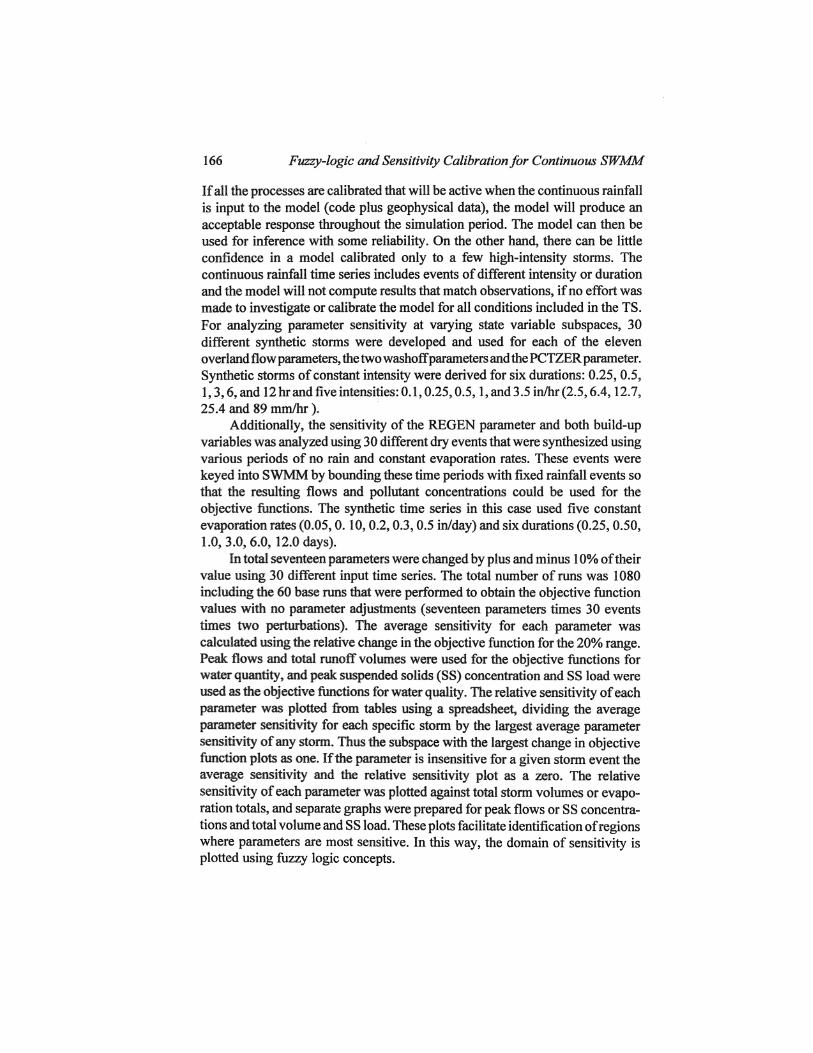
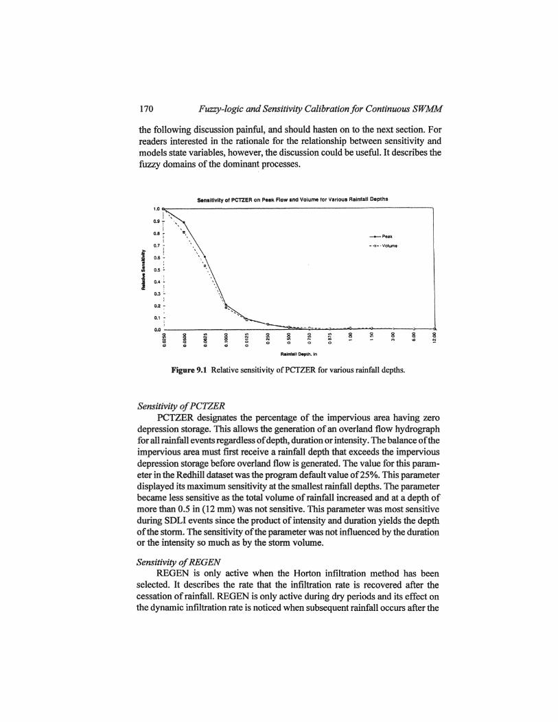
Each parameter was adjusted plus and minus 1 OOAtofits value and the dataset run in the model for 30 different wet or dry events. A spreadsheet was used to prepare sensitivity plots - for PCTZER see Figure 9.1. Casual readers win find
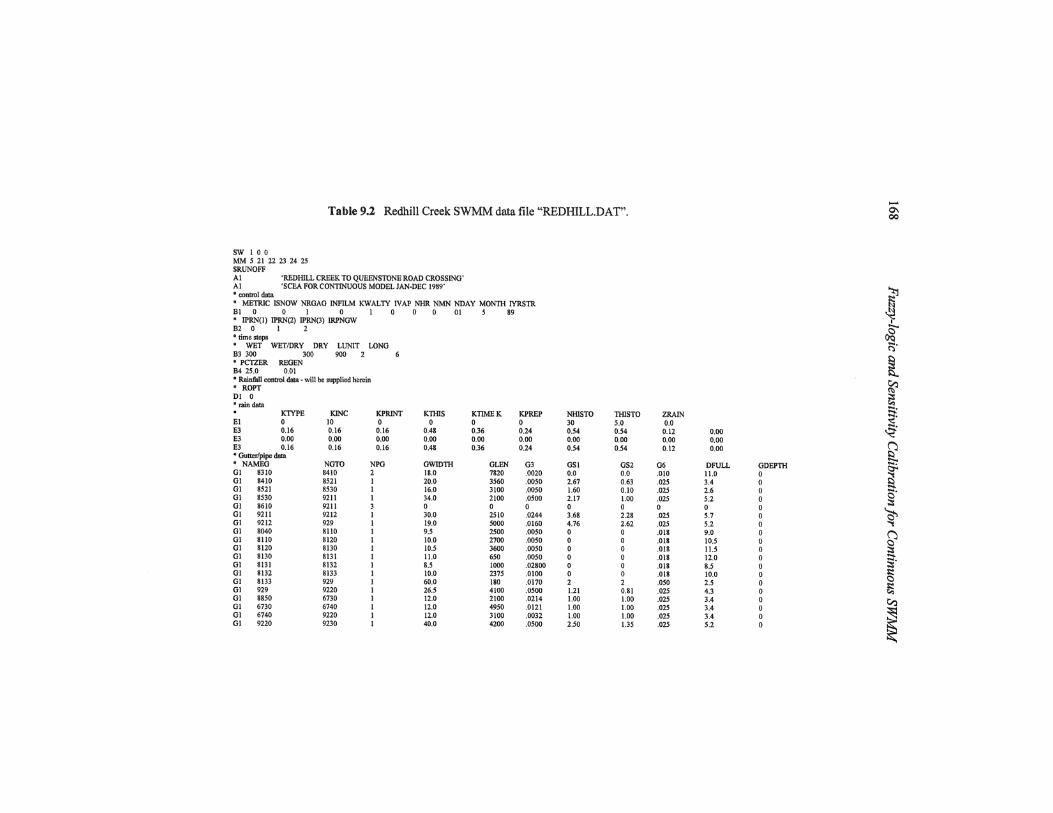
Table 9.2 Redhill Creek SWMM data file "REDHILL.DAT".
SW 100 MM 5 21 22 23 24 25 SRUNOFF Al 'REOHlLL CREEK TO QlJJiENSTONIl ROAD CROSSING' Al 'SCFAFORCONTINUOUS MODJ3L1AN·DEC 1989' $ control diIta • METRIC lSNOW NRGAO INFlLM KWAt:rv IVAP NHR !>.'MN NDAY MONTH IYRSTR Bl 0 0 I 0 1 () 0 0 01 5 89 • lPRN(I) lPRi'l(2) IPRN(3) IRPNOW 112 0 1 2 • time steps • WET WETIDRY DRY LUNlT LONG 53 300 300 900 2 • PC1ZER REGEN B4 25,0 0.01 • Rainfull """""Idola· "m be ,upplied he.,in • ROPT Dl 0 .. rain data
EI E3 E3 E3
KTYP!l 0 0,16 0.00 0.16
• Gutter/pip< data • NAMEG Gl 8310 01 8410 Gl 8521 Gi 8530 Gl 86JO 01 9211 01 9212 01 8040 Gl SilO Gl 8120 Gl 8130 Gl 8131 Gl 8132 OJ 8m 01 929 Gl 8850 Gl 6730 Gl 6740 GI 9220
KlNC KPRINT JO 0 0.16 0,16 0,00 0,00 0,16 0,16
NOTO NPG 8410 2 8521 I 8530 I 9211 i 9211 3 9212 I 929 I 8110 1 8120 I 8130 I 8131 I 8132 I 8133 I 929 1 9220 I 6730 ! 6740 I 9220 1 9230 1
KTHlS KTIM!lK 0 0
0,48 0.36 0,00 0,00 O.4~ 0,36
GWlD11I OLEN 18,0 7820 20,0 3560 16,0 3100 34,0 2100 0 0 30,0 2510 19.0 5000 9.5 2500 10,0 2700 10.5 3600 11.0 650 8.5 1000 10,0 2375 60,0 180 26,5 4100 12.0 2100 12,0 4950 12,0 3100 40,0 4200
KPREP 0 0.24 0,00 0.24
03 ,0020 ,0050 ,0050 ,0500 0 ,0244 ,0160 ,0050 ,0050 ,0050 ,0050 ,02800 ,0100 ,0170 ,0500 ,0214 ,0121 ,0032 .0500
NHlSTO THlSTO 30 5.0 0.54 0.54 0,00 0,00 0.54 0,54
OSI OS! 0,0 0.0 2,67 0,63 1.60 0,10 2,17 1.00 0 0 3,68 2,28 4,76 2,62 0 0 0 0 0 0 0 0 0 0 0 a 2 2 1.21 0,81 1.00 1.00 1.00 1.00 1.00 1.00 2.50 1.35
ZRAIN 0,0
0,12 0,00 0,00 0,00 0,12 0,00
06 DFULL .010 11.0 ,025 3.4 ,025 2,6 ,025 5,2 0 0 .025 5,7 .025 5.2 ,018 9,0 ,018 10.5 ,018 ll.s ,018 12.0 ,018 g,5 ,018 10,0 ,050 2.5 .025 4.3 ,025 3,4 ,025 3.4 .025 3,4 ,025 5,2
ODEPTH 0 0 0 0 0 0 0 0 0 0 0 0 0 0 0 0 0 0 0
...... 0'\ 00
~
~ , C'
I)Q ~.
§ I::l...
~ ~ .... ~ ~ ~ ~ ~ -§. ~ "t
~ .... ;:;. § !:i V:l
~
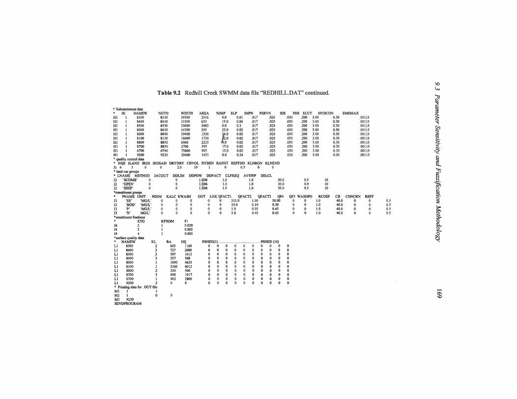
Table 9.2 Redhill Creek SWMM data file "REDHILL.DAT" continued,
'" Subcatchment data JK NAMEW NGTO WIDTH AREA %IMP SLP IMPN PERliN IDS PDS SUCT HYDCON SMDMAX
HI I 8300 8310 39300 2516 0.0 0.01 .017 .025 .050 .200 3.00 030 .00115 HI I 8400 8410 31500 633 \5.0 0.04 .017 .025 .050 .200 3.00 0.30 .00115 HI 1 8500 8530 30000 3483 0.0 0.2 .017 .025 .050 .200 3.00 0.30 .00115 HI I 8600 8610 14300 355 23.0 0.02 .017 .025 .050 100 3.00 0.30 ,OOil5 HI I 8000 8040 30400 1336 ~o om .017 .025 .050 .200 3.00 030 .00115 HI I 8100 8130 16600 1736 2.0 0.02 .017 .025 .050 .200 3.00 0.30 .oow HI I 8800 8850 6060 2235 .0 0.02 .017 .025 .050 100 3.00 0.30 .00115 HI 1 8700 8850 2700 595 17.0 0.02 .017 .025 .050 .zoo 3.00 030 .00115 HI I 6700 6740 75600 997 15.0 0.Q2 .017 .025 .oso .200 3.00 030 .OOllS HI I 9200 9220 20400 1471 0.0 0.24 .017 .025 .uso .200 3.00 0.30 .oom , quality control data , NQS lLAND IROS IROSAD DRYDRY CBVOL RYBSN RAlNIT REFFDD KLNBGN KLNEND JI 4 3 0 0 2.0 19 I 0 0.5 0 0 '* land use groups
• LNAME METHOD JACOUT DDLIM DDPOW DDFACT CLFREQ AVSWP DSLCL 12 'SCOMB' 0 0 I.E06 1.0 1.0 30.0 O.S 10 )2 'OPEN' 0 0 I.E06 1.0 1.0 30.0 0.9 10 J2 'SSEP' 0 0 I.E06 1.0 1.0 30.0 05 10 .. constituent groups · PNAME UNIT NDIM KALC KWASH OUT LNKQFACTI QFACT2 QFACTl QF4 QF5 WASHPO RCOEl' CB CONCRN REFF 13 '55' 'MOIL' 0 0 0 0 0 315.0 1.00 50.00 0 0 1.0 40.0 0 0 13 'BOD' 'MOIL' 0 0 0 0 0 10.0 0.10 0.30 0 0 1.0 40.0 0 0 13 'p' <MOIL' 0 0 0 0 0 1.0 0.05 0.45 0 0 1.0 40.0 0 13 'N' MOIL' 0 0 0 0 0 3.0 0.45 0.45 0 0 1.0 40.0 0 ,. constituent frncti.ons
KTO KFROM FI )4 2 1 0.020 J4 3 I 0.002 J4 4 1 0.005 *' surface quality data · NAMEW KL SA OQ PSHF,D(I) ....... ... PSRED (10) LI 8300 2 603 1I60 0 0 0 0 II 0 0 0 0 0 LI 8400 3 727 2000 0 0 0 0 0 II 0 0 0 0 Ll 8500 2 587 1612 0 0 0 0 0 0 0 0 0 0 LI 8600 3 207 568 0 0 0 0 0 0 0 II 0 0 Ll 8000 I 1690 4655 0 0 0 0 0 II 0 0 0 0 LI 8100 I 2186 6012 0 0 a 0 0 0 0 0 0 0 LI 8800 2 240 560 0 0 0 0 0 II 0 0 0 0 LI 3700 3 698 1917 0 0 0 0 0 0 0 0 0 0 1..1 6700 I 902 2800 0 0 0 0 0 0 0 0 0 0 LI 9200 2 0 0 0 0 0 0 0 0 0 0 0 0 • Printing data for .OUT file Ml I I M2 I 0 M3 9230 SENDPROGRAM
0.5 0.5 0.5 0.5
'0 ~
f t1:> ~ "t
~ ~ 5: ~
~
~ ~ I>i ~ (')
~ §'
~ S-o ~ C3'" ~
,.... 0\ \0
170 Fuzzy-logic and Sensitivity Calibration for Continuous SWMM
the following discussion painful, and should hasten on to the next section. For readers interested in the rationale for the relationship between sensitivity and models state variables, however, the discussion could be useful. It describes the fuzzy domains of the dominant processes.
Sensitivity of PCTZI!R on Peek Flow and Volume far Various Rainfall Depths
1.0
I , OJIr
i 0.8 • , -..-P .. k
I 0.7 - --o-'VoNme
f , !
0.8-,
Q.5~
I ,
0.4 i I
0.3 " I
0.2 7
0.1 ~
i 0.0
! ! i ~ ..
! ~ !1! '" a .. :;; c; .. co Q .. .; .. 8 .., a ...
_iDo!Mh.in
Figure 9.1 Relative sensitivity ofPCTZER for various rainfall depths.
Sensitivity of PCTZER PCTZER designates the percentage of the impervious area having zero
depression storage. This allows the generation of an overland flow hydrograph for all rainfall events regardless of depth, duration or intensity. The balance of the impervious area must first receive a rainfall depth that exceeds the impervious depression storage before overland flow is generated. The value for this parameter in the Redhill dataset was the program default value of25%. This parameter displayed its maximum sensitivity at the smallest rainfall depths. The parameter became less sensitive as the total volume of rainfall increased and at a depth of more than 0.5 in (12 mm) was not sensitive. This parameter was most sensitive during SDLI events since the product of intensity and duration yields the depth of the storm. The sensitivity of the parameter was not influenced by the duration or the intensity so much as by the storm volume.
Sensitivity of REGEN REGEN is only active when the Horton infiltration method has been
selected. It describes the rate that the infiltration rate is recovered after the cessation of rainfall. REGEN is only active during dry periods and its effect on the dynamic infiltration rate is noticed when subsequent rainfall occurs after the
9.3 Parameter Sensitivity and Fuzzijication Methodology 171
dry period. The sensitivity of this parameter requires a range of durations and evaporation rates to describe the dry inter-event period. The value for this parameter in the Redhin dataset was 0.01 sec-I. This parameter displayed its maximum sensitivity for medium inter-event durations of one to three days. The parameter became insensitive after a duration of six days of no rain. The evaporation rates had no impact on the sensitivity of this parameter using peak flow as the objective function. Minimal sensitivity was seen f or different evaporation rates using runoff volume as the objective function. This parameter never displayed more than a 0.7% change in any objective function for a 10% change in the variable. This parameter was directly influenced by the duration of no rain.
Sensitivity of WIDTH WIDTH is used to assign an average or effective width of overland flow on
the subcatchment, assuming sheet flow on the subcatchment for its non-linear reservoir routing. WIDTH is a measure of overland flow width for both the pervious and impervious areas. Larger subcatchment widths result in faster catchment response and are representative of highly drained areas. Smaller subcatchment widths mean longer overland flow lengths, longer response time and are representative of open areas v.ithout well defined surface and engineered drainage systems. The value for this parameter in the Redhill dataset ranged from 2700 to 39300 ft(823 to 12000m).Thetwocorrespondingsubcatchmentsforthis low and high WIDTH value had catchment areas of 595 and 2516 acres (242 and 1023 ha) and percent imperviousness of17.0 and 0.0 respectively. This parameter displayed its maximum sensitivity at the smallest rainfall totals but some sensitivity was seen for all rainfall depths. The parameter became less sensitive as the total volume of rainfall increased and at a depth of more than 0.50 was markedly less sensitive. Tlus parameter was most sensitive during SOLI events and SDHI events. A second region of sensitivity for SOl-II events was also discovered. This is when pervious area runoff contributed to the overall peak and runoffvolumetotals. For the two stonnsof3.5 inlhr(89mmlhr) and 0.25 and 0.5 0 hours duration the WIDTH parameter was as sensitive as it was for most intensities atthe SDs. WIDTH was not sensitive for durations in excess oD hours except for MI storms with respect to the volume of runoff. Generally the parameter was sensitive when a new source of overland flow contributed to the total runoff, such as a pervious area with depression storage. At the smallest rainfall intensities and volumes, overland flow consists of only overland flow on the impervious area without any depression storage. At rainfall depths exceeding the impervious area depression storage the impervious area contributed to the total runoff and the WIDTH parameter was sensitive. Finally, at high intensities above the infiltration rate the WIDTH parameter was again sensitive as pervious area overland flow became a significant portion of the total flow. Some sensitivity
172 Fuzzy-logic and Sensitivity Calibration for Continuous SWMM
although less than the others was also noticed at LDMI as the infiltration rate was reduced to a rate less than the rainfall intensity and overland flow occurred on the pervious area.
Sensitivity of WAREA W AREA is used to designate the total area of each subcatchment in the
watershed. Impervious areas are described by a percentage of the total area and thus increasing or decreasing the W AREA parameter will adjust the total area of the subcatchment and not effect the ratio of impervious and pervious areas. This parameter is not often considered to be a suitable parameter for calibration because of the accuracy used in survey and GIS techniques. However, W AREA is a measure of the hydraulically effective area. If a portion of the subcatchment although clearly within a defined subcatchment boundary does not directly connect to the drainage network, only the area contributing to the overall measured runoff should be counted as the area of the subcatchment. For example, a sag in the landscape, that drains only by infiltration and no groundwater flow is being modeled, should be excluded from the area. In addition, the sensitivity of the subcatchment area can show the location of hydraulic limitation in a sewer shed when a proportional amount of flow is not seen for an increase or decrease in W AREA. Theoretically there should be a 10% increase in runoff for a 10% increase in area. Values for the subcatchment areas in the Redhill dataset ranged from 355 to 3463 acres (144 to 1408 ha). This parameter displayed its maximum sensitivity at the smallest rainfall totals where there was an even larger increase in peak flow than parameter change. At most other rainfall storms the sensitivity was nearly 1: 1 with a 10% increase in peak flows and runoff volume for a 10% increase in the W AREA parameter. Correspondingly, the peak flow and runoff volumes decreased by l00fc, for a decrease in the WAREA parameter. The parameter was equally sensitive for all ranges of storms except at very HI and high nmoffvolumes. At these times the model was hydraulically controlled and the runoff rates were reduced at the outfall by limited hydraulic capacity of conduits and excess flows were simulated with artificial storage at inlets. This was found to be at depths of more than 1.5 in (38 mm) and rainfall rates of3.5 inIhr (89 mmJhr). During simulations when more flow was generated than the hydraulic system can handle, RUNOFF stQres water at the upstream inlets or junctions until there is capacity later in the simulation for these flooded volumes to be entered into the system. This method mayor may not mimic the physical system being modeled. mITRAN offers alternatives to modeling hydraulics and surcharge.
Sensitivity of Percent Impervious The percent impervious (%INT) parameter is used to assign a portion of the
total subcatchment area as impervious area and hence not subjected to infiltration losses .. This area allows the complete generation of all rainfall to overland flow
9.3 Parameter Sensitivity and Fuzzijication Methodology 173
for rainfall amounts greater than the depression storage. Additionally, some of this impervious area can have no depression storage and is designated by PCTZER as discussed earlier. Hence, a larger percent impervious or total area will also increase the total area for the impervious area without depression storage. The value for this parameter among all subcatchments ranged from OOAt to 24%. This parameter displayed equal sensitivity of nearly a 1: 1 correlation while there was only overland flow on the impervious areas. At high rainfall intensities and LDMI where overland flow was generated on the pervious area, the sensitivity was significantly diminished. At these times the impervious area runoffbecame less than 100% of the total runoff. The domain of sensitivity for this parameter was all LIMI andSDMI storms. The parameterdidnotbecome less sensitive as the total volume of rainfall increased except when total runoffwas hydraulically limited by the sewer network. This parameter was most sensitive during SDLI events. The sensitivity of the parameter was influenced by increased duration for all storms with intensities greater than the minimum infiltration rate and duration long enough to cause overland flow on the pervious area. Similar sensitivity was displayed using peak flows or runoff volumes as the objective function.
Sensitivity o!WSLOPE WSLOPE is used in the SWMM program to assign an average slope for the
idealized subcatchment The same slope is common to all surfaces on the subcatchment (pervious and impervious). If the physical slopes on each surface are significantly different, two separate subcatchments should be considered, one subcatchment of a given slope for the entire pervious area and another for the entire impervious area. Alternatively, some small differences in overland flow caused by having different slopes for each surface can be incorporated by using suitable values of roughness for each surface. Larger WSLOPE values resulted in a faster response to rainfall, larger peak flows and runoff volumes in this analysis. The value for this parameter ranged from 0.01 to 0.24 ftlft. This parameter displayed its maximum sensitivity for SDLI. However, the parameter was sensitive for all rainfall intensities of SD. The parameter became less sensitive as the duration increased and at a duration of more than 1.0 hr was markedly less sensitive. Some sensitivity was found for all events with runoff volume as the objective function, but no sensitivity was discovered for durations of more than 3 hr with peak flow as the objective function. This parameter was not highly sensitive even at SDLI. In this case a 10% change in the parameter resulted in a 2.7% change in the peak flow and a 2.0% change in the runoff volume. Generally the parameter was sensitive for SDs. For these storms ahigher slope resulted in larger peak flows and volumes since the depth of water on the idealized catchment builds up over time.
174 Fuzzy-logic and Sensitivity Calibration jor Continuous SWMM
Sensitivity oj IMPERN IMPERN is used to assign a Manning's roughness to the impervious area
of the subcatchment. The subcatchment width and the slope are common to both the pervious and impervious area. Allowing different roughness values for each surface permits the runoff hydrographs for each surface to have different resulting time to peaks and hydrograph shapes. Impervious areas respond to aU rainfall intensities and volumes if some of the impervious area has no depression storage. Correspondingly, the domain for the sensitivity of the IMPERN parameter is when the overland flow on the impervious area is the dominant process. In addition, the sensitivity of the IMPERN parameter should decrease as overland flow on the pervious area becomes a larger portion of the total sub catchment response. The value of the INTERN for each subcatchment in the RedhiH dataset was 0.017 although the model allows different IMPERN for each subcatchment. This parameter displayed its maximum sensitivity at the smallest rainfall totals where only overland flow was occurring from the impervious area without depression storage. Unlike all of the previously discussed parameters, when this parameter was increased the peak flow and runoff volume decreased. This follows intuition because a rougher surface impedes the overland flow. At its most sensitive state a 10% change in the IMPERN parameter resulted in a 5.5% change in peak flow and a 4.0% change in the runoff volume. The parameter sensitivity was very uniform with respect to duration and intensity. As the intensity increased and the duration increased the sensitivity reduced for both peak flow and runoff volume. Generally the parameter was sensitive for SD and MD and LI and ML The sensitivity dropped off sharply above 1 hour duration and 0.5 inlhr (12 mmlhr). The diminished sensitivity for this parameter at longer durations and intensities is attributed to the increase of the overland flow on the pervious area as a portion of the total flow.
Sensitivity ojPERVN PERVN is used to assign Manning's roughness to the pervious area. Just as
was the case for the impervious area roughness. an increase in this parameter allows a longer time to peak and a flatter hydro graphs for the pervious area. Pervious areas only generate runoff in SWMM when the depression storage has been exceeded and the rainfall rate is greater than the infiltration rate. Correspondingly, PERVN will be most sensitive when the overland flow on the pervious area is a dominant process. Additionally, the domain should not include SD low and M1 events. In addition, the sensitivity ofPERVN should be at its highest at the onset of overland flow on the pervious area. The value of PER VN for each subcatchment in the Redhill dataset was 0.025 although the model allows different PERVN for each subcatchment as was the case for IMPERN. This parameter displayed its maximum sensitivity for HI SD rainfall. Unlike the IMPERN parameter which displayed sensitivity for all storms this parameter did
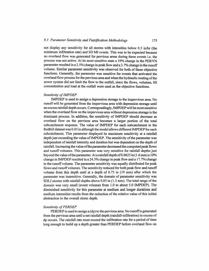
9.3 Parameter Sensitivity and Fuzzijication Methodology 175
not display any sensitivity for all storms with intensities below 0.5 inlhr (the minimum infiltration rate) and SD MI events. This was to be expected because no overland flow was generated for pervious areas during these events i.e. the process was not active. At its most sensitive state a 10% change in the PERVN parameter resulted in a 2.5% change in peak flow and a 3.7% change in the runoff volume. Similar parameter sensitivity was observed for both of these objective functions. Generally, the parameter was sensitive for events that activated the overland flow process for the pervious area and when the hydraulic routing of the sewer system did not limit the flow to the outfall. since the flows, volumes, SS concentration and load at the outfall were used as the objective functions.
Sensitivity of IMPDEP IMPDEP is used to assign a depression storage to the impervious area. No
runoff wm be generated from the impervious area with depression storage until an excess rainfall depth occurs. Correspondingly, IMPDEP will be most sensitive when the overland flow on the impervious area without depression storage is the dominant process. In addition, the sensitivity of IMPDEP should decrease as overland flow on the pervious area becomes a larger portion of the total subcatchment response. The value of IMPDEP for each subcatchment in the Redhill dataset was 0.05 in although the model allows different IMPDEP for each subcatchment. This parameter displayed its maximum sensitivity at a rainfall depth just exceeding the value ofIMPDEP. The sensitivity of the parameter was independent of rainfall intensity and duration but was dependent on the depth of rainfalL Increasing the value of the parameter decreased the computed peak. flows and runoff volumes. This parameter was very sensitive for rainfall depths just beyond the value of the parameter. AtarainfaU depth of 0.0625 in (1.6 mm)a 10% change in IMPDEP resulted in a 24.5% change in peak flow and a 17.7% change in the runoff volume. The parameter sensitivity was equally distributed for peak flows and runoff volumes. The sensitivity reduced for both peak. flow and runoff volume from this depth until at a depth of 0.75 in (19 mm) after which the parameter was insensitive. Generally, the domain of parameter sensitivity was SDU storms with rainfall depths above 0.05 in (1.3 mm). The total range of the domain was very small (event volumes from 1.0 to about 5.0 IMPDEP). The diminished sensitivity for this parameter at medium and longer durations and medium intensities results from the reduction of the relative value of this initial abstraction to the overall storm depth.
Sensitivity of PERDEP PERDEP is used to assign a (dp) to the pervious area. No runoffis generated
from the pervious area until a net rainfall depth (rainfall-infiltration) in excess of dp occurs. The rainfall rate must exceed the infiltration rate for a period of time long enough to build up a depth greater than PERDEP before overland flow on
176 Fuzzy-logic and Sensitivity Calibration for Continuous SWMM
the pervious area. PERDEP is most sensitive when the overland flow on the pervious area becomes a dominant process. In addition, the sensitivity of PERDEP should decrease as overland flow on the pervious area increases as a portion of the total subcatchment response since PERDEP acts as a fixed initial abstraction of rainfall. However, in the case of an actual rainfall storm the depth on the watershed is dynamic with the depth increasing when rainfall exceeds infiltration and falling when the inverse is true. The value ofPERDEP for each subcatchment in the Redhill dataset was 0.20 in. This parameter displayed its maximum sensitivity for SDHI and LDMI events. These two regions of input variable subspaces activated overland flow over the pervious areas. There was no sensitivity of the parameter for events with less than 0.875 in (22 mm) ofrain or events with less than 0.50 inlhr rainfall intensity. The sensitivity was dependent on rainfall intensity and duration because all intensities had to be greater than the minimum infiltration rate and have a duration long enough to develop a depth on the watershed more than PERDEP. In a similar fashion to IMPDEP increasing the value of the parameter decreased the peak flow and runoff volumes. The parameter was most sensitive for the highest intensity shortest duration event with a 10% change in PERDEP causing a 4.0% change in peak flow and a 6.6% change in the runoff volume.
Sensitivity ofWLMAX WLMAX is used to assign an initial infiltration rate for the pervious area of
the subcatchment when the Horton infiltration option is used. No runoff is generated from the pervious area unless the rainfall rate is more than the infiltration rate and the depression storage on the pervious area is filled. The infiltration rate in SWMM is dynamic, using the Horton method has the infiltration rate decay exponentiallythroughoutthe storm from the WLMAX rate to the WLMIN rate using the DECAY parameter to describe the rate of infiltration decay. The sensitivity ofWLMIN and DECAY is described after this section. High WLMAX rates lower the peak flows and volumes of runoff as more rainfall is allowed to infiltrate. Correspondingly, the WLMAX parameter will be most sensitive when the overland flow on the pervious area is dominant. The value ofWLMAX was 3.00 inIhr for each subcatchment in the Redhill dataset. Individual infiltration parameters can be used for each subcatchment, each is a lumped parameter, or an effective rate for an individual subcatchment. This parameter shared the same domain of sensitivity as PERDEP with the sensitivity being about twice as great. This parameter displayed its maximum sensitivity for HI SD and LD MI events. In these two regions the rainfall activated the overland flow over the pervious areas. There was no sensitivity of the parameter for events with less than 0.750 in of rain or events with less than 0.50 inIhr. The sensitivity was dependent on rainfall intensity and duration because all intensities had to be greater than the minimum infiltration rate and have a duration long enough to
9.3 Parameter Sensitivity and Fuzzijication Methodology 177
develop a depth on the watershed exceeding PERDEP. The parameter was most sensitive for the highest intensity shortest duration event with a 10% change in PERDEP causing a 9.3% change in peak flow and a 12.7% change in the runoff volume.
Sensitivity of WLMIN WLMIN is used to assign a minimum infiltration rate when the Horton
infiltration option is used. High WLMIN rates lowers the peak flows and volumes of runoff since more rainfall is allowed to infiltrate. For LOs and large storm volumes the infiltration rate will reduce down to or near the minimum infiltration rate described by WLMIN. Correspondingly. WLMIN will be most sensitive when the overland flow on the pervious area is the dominant process and infiltration has reached this minimum. The value ofWLMIN was 0.30 inlhr for each subcatchment in the Redhill dataset. This parameter was sensitive for very large storm volumes. It was most sensitive for storms of 1.5 to 6 in (38 to 152 mm) in depth, and for the MI LD events. Although some sensitivity was seen for HI LD events these generated extremely high flows and the runoff obtained at the outfan was limited by the conveyance system. As the intensity increased above the minimum infiltration rate and the duration increased, parameter sensitivity decreased. This showed that sensitivity was a maximum with storm intensities just above the minimum infiltration rate. There was no sensitivity of the parameter for events with less than 0.750 in of rain or events with an intensity of less than 0.50 inlhr. The sensitivity was dependent on rainfall intensity and duration because all intensities had to be greater than the minimum infiltration rate and have a duration long enough to saturate the soil and reduce the infiltration rate to less than the rainfall rate. The parameter was most sensitive for the lowest MI with the shortest duration that lowered the infiltration rate to or near WLMIN. For the case of the maximum sensitivity using peak flow and runoff volume as objective functions a 10% change in the WLMIN parameter resulted in a 13.9% change in peak flow and a 18.4% change in the runoff volume.
Sensitivity of DECAY DECAY is used to describe the rate that the Horton infiltration rate will
decrease from WLMAX to WLMIN. The infiltration rate will decay over time for aU cases where the rainfall rate is greater than the WLMIN. Thus no sensitivity will be seen for this parameter for events with the rainfall rate less WLMIN. Additionally, for events when the rainfall rate exceeds the dynamically changing infiltration rate and the depth of water on the subcatchment equals or exceeds PERDEP there will be flow on the pervious area and sensitivity gradients can be calculated using the peak flow and runoff volume for this parameter. High DECA Y rates raise the peak flows and volumes of runoff as less rainfall is allowed to infiltrate with the infiltration rate decreasing faster. Correspondingly
178 Fuzzy-logic and Sensitivity Calibration for Continuous SWMM
the DECA Y parameter will be most sensitive when the overland flow on the pervious area is the dominant process. The value of DEC A Y was 0.00115 s-I for each subcatchment in the RedhiH dataset. This parameter was sensitive in the identical input parameter subspaces as WLMAX and WLMIN with the sensitivity gradients in the case of DECA Y being opposite in sign. This parameter displayed its maximum sensitivity for SDm and LDMI events. These two regions of input variable subspace activated overland flow over the pervious areas. There was no sensitivity ofthe parameter for events with less than 0.750 in of rain or events with intensities less than 0.50 inlhr. The sensitivity was dependent on rainfall intensity and duration because all intensities had to be greater than the minimum infiltration rate and be of sufficient duration to develop a depth on the watershed greater than PERDEP. The parameter was most sensitive for the highest intensity shortest duration event with a 10% change in PERDEP resulting in a 4.2% change in peak flow and a 7.6% change in the runoff volume.
Sensitivity of W ASHPO SWMM can use an exponential washoff equation for the prediction of
dynamic runoff concentration. Two variables are used to describe the washoff of available pollutants from the catchment. W ASHPO is the exponent in the washoffequation. For the sensitivity analysis of this study only the SS concentration and load were used as objective functions, all of the remaining water quality parameters would have similar sensitivity. A washoff exponent of more than 1.0 is generally used to model sediment source constituents and a value of less than 1.0 is often used to model dissolved constituents whose concentration diminishes strongly with increasing flow rate. A value of 1.0 (used in the Redhm Creek example) would cause the equation to be linear. The same set of storm events tbatwere used for all of the hydrology parameters was used for the analysis of WASHPO and RCOEFF (the coefficient in the washoff equation). The difference in the analysis is that the peak SS concentration and load are used as objective functions to measure sensitivity instead of the peak flow and runoff v01ume. For aU cases the number of dry days before the start of each event used in the sensitivity analysis was 2.0 days. DRYDA Y initializes the model with a ftxed amount of pollutants on the subcatchment described by the buildup equation discussed later. The value of the WASHPO for SS was 1.0 in the Redhill dataset A deviation from 1.0 results in a nonlinear equation and correspondingly the parameter is very sensitive. Individual W ASHPO parameters are used for each pollutant. In the case ofthe Redhill Creek dataset the three other pollutants also used a value of 1.0. Washoff was most sensitive for the SD LI storms. Decreasing sensitivity was found with increased storm depth and the sensitivity of the parameter to load was very small beyond 0.750 in ofrainfaU. However, using peak concentration as the objective function the parameter was sensitive for
9.3 Parameter Sensitivity and Fuzzijication Methodology 179
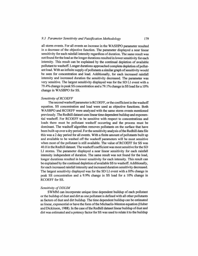
all storm events. For all events an increase in the WASHPO parameter resulted in a decrease of the objective function. The parameter displayed a near linear sensitivity for each rainfall intensity regardless of duration. The same result was not found for the load as the longer durations resulted in lower sensitivity for each intensity. This result can be explained by the continual depletion of available pollutant to washoff. Longer durations approached complete depletion of pollutant load. With an infinite supply of pollutants a similar graph of sensitivity would be seen for concentration and load. Additionally, for each increased rainfall intensity and increased duration the sensitivity decreased. The parameter was very sensitive. The largest sensitivity displayed was for the SD LI event with a 79.4% change in peak SS concentration and a 79.1 % change in SS load for a 10% change in W ASBPO for SS.
Sensitivity of RCOEFF The second washoff parameter is RCOEFF, or the coefficient in the washoff
equation. SS concentration and load were used as objective functions. Both W ASBPO and RCOEFF were analyzed with the same storm events mentioned previously. The RedWU dataset uses Iineartime dependent buildup and exponential washoff. For RCOEFF to be sensitive with respect to concentrations and loads there must be pollutant washoff occurring and the process must be dominant. The washoff algorithm removes poHutants on the surface that have been built-up over a dry period. F or the sensitivity analysis ofihe Redhill data me this was a 2 day period for aU events. With a finite amount of pollutants built up and available to be washed off the washoff parameters wiH be most sensitive when most of the pollutant is still available. The value of RCOEFF for SS was 40.0 in the Redhill dataset. The washoff coefficient was most sensitive for the SD LI storms. The parameter displayed a near linear sensitivity for each rainfall intensity independent of duration. The same result was not found for the load, longer durations resulted in lower sensitivity for each intensity. This result can be explained by the continual depletion of available SS to washoff. Additionally, for each increased rainfall intensity and increased duration sensitivity decreased. The largest sensitivity displayed was for the SD LI event with a 10% change in peak SS concentration and a 9.9% change in SS load for a 10% change in RCOEFF for SS.
Sensitivity of DDLIM SWMM can incorporate unique time dependent buildup of each pollutant
or the buildup of dust and dirt as one pollutant is defmed with all other pollutants as factors of dust and dirt buildup. The time dependent buildup can be estimated as linear, exponential or have the form of the Michaelis-Menton equation (Huber and Dickinson, 1988). In the case ofthe RedhiH dataset linear buildup of dust and dirt was estimated and a potency factor for SS was used to relate it to the buildup
180 Fuzzy-logic and Sensitivity Calibration for Continuous SWMM
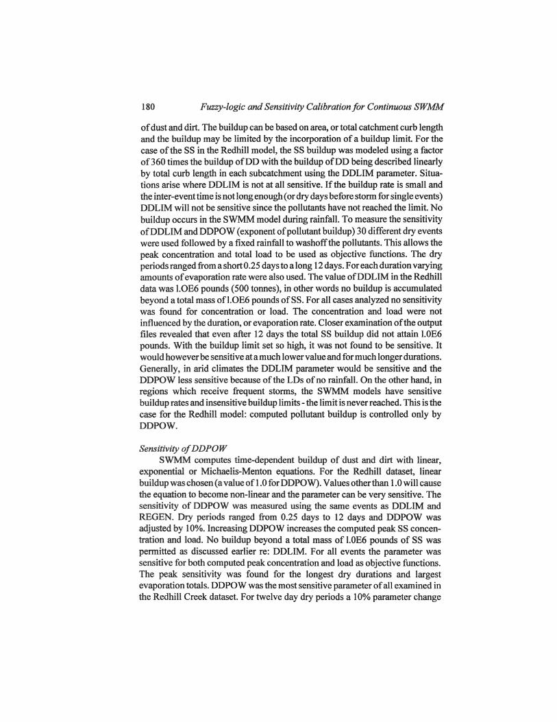
of dust and dirt. The buildup can be based on area, or total catchment curb length and the buildup may be limited by the incorporation of a buildup limit. For the case of the SS in the Redhill model, the SS buildup was modeled using a factor of360 times the buildup ofDD with the buildup of DO being described linearly by total curb length in each subcatchment using the OOLIM parameter. Situations arise where DDLIM is not at all sensitive. If the buildup rate is small and the inter-event time is not long enough (or dry days before storm for single events) OOLIM will not be sensitive since the pollutants have not reached the limit. No buildup occurs in the SWMM model during rainfall. To measure the sensitivity of DO LIM and ODPOW (exponent of pollutant buildup) 30 different dry events were used followed by a fIxed rainfall to washoffthe pollutants. This allows the peak concentration and total load to be used as objective functions. The dry periods ranged from a short 0.25 days to a long 12 days. For each duration varying amounts of evaporation rate were also used. The value ofOOLIM in the Redhill data was LOE6 pounds (500 tonnes), in other words no buildup is accumulated beyond a total mass ofl.OE6 pounds ofSS. For aU cases analyzed no sensitivity was found for concentration or load. The concentration and load were not influenced by the duration, or evaporation rate. Closer examination of the output files revealed that even after 12 days the total SS buildup did not attain 1.0E6 pounds. With the buildup limit set so high, it was not found to be sensitive. It would however be sensitive at a much lower value and for much longer durations. Generally, in arid climates the DDLIM parameter would be sensitive and the DDPOW less sensitive because ofthe LOs of no rainfall. On the other hand, in regions which receive frequent storms, the SWMM models have sensitive buildup rates and insensitive buildup limits - the limit is never reached. This is the case for the Redhm model: computed pollutant buildup is controlled only by DOPOW.
Sensitivity of DDPOW SWMM computes time-dependent buildup of dust and dirt with linear,
exponential or Michaelis-Menton equations. For the Redhm dataset, linear buildup was chosen (a value of 1.0 for DOPOW). Values other than 1.0 will cause the equation to become non-linear and the parameter can be very sensitive. The sensitivity of DDPOW was measured using the same events as ODLIM and REGEN. Dry periods ranged fi'om 0.25 days to 12 days and DDPOW was adjusted by l(WG. Increasing ODPOW increases the computed peak SS concentration and load. No buildup beyond a total mass of LOE6 pounds of SS was permitted as discussed earlier re: DOLIM. For aU events the parameter was sensitive for both computed peak concentration and load as objective functions. The peak sensitivity was found for the longest dry durations and largest evaporation totals. ODPOW was the most sensitive parameter of all examined in the RedhiH Creek dataset. For twelve day dry periods a 10% parameter change
9.5 Manual Calibration Procedure 181
resulted in a 187.3% change in the computed peak concentration of SS and a 159. % change in the computed SS load. Evaporation rates had only a very small influence in the concentrations and loads; greater input rates of evaporation caused higher computed concentrations and loads. The sensitivity of the parameter increased dramatically for durations beyond I day. The buildup limit was set so high in this dataset that there was no limiting effect on the sensitivity of DDPOW.
9.4 Fuzzification of the Hydrological Processes
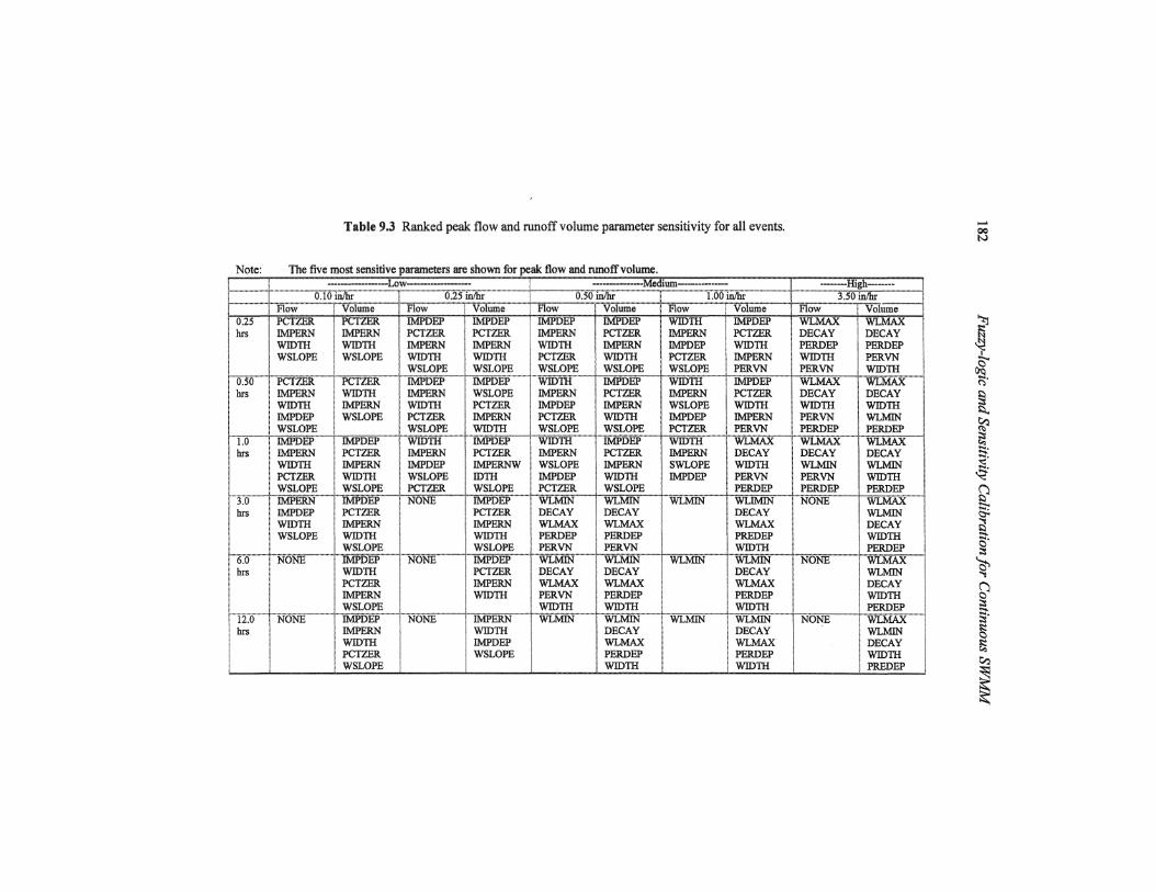
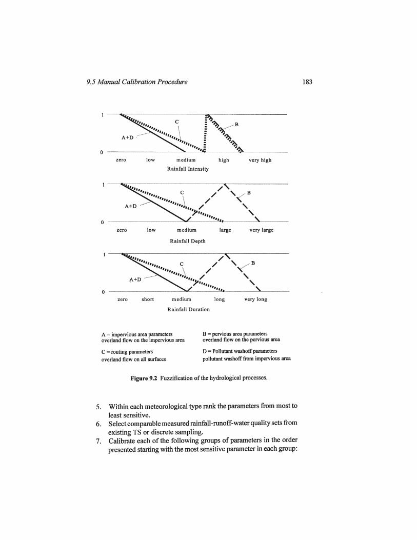
Hundreds of processes are modeled in the entire SWM.,.\.i suite. However, this study was limited to a discussion of the RUNOFF processes modeled in the Redhill dataset, a total of seventeen parameters. The parameters can be grouped by macroscopic processes such as overland flow over the pervious area or pollutant buildup. In this section the absolute parameter sensitivity is compared for parameters sensitive to a group of meteorological events. The sensitivity is ranked in Table 9.3, from most sensitive to least, for storms ofSD,MD, or LD and for LI, MI and HI. Using the sensitivity results, the sensitivity of the foHowing groups of parameters are shown in fuzzy terms in Figure 9.2.
Note: Separate plots are used for each of the foHowingrainfall descriptions: depth, duration, and intensity.
9.5 Manual Calibration Procedure
It is not feasible to perform a sensitivity analysis or a calibration exercise on a continuous SWMM model. Continuous models are not calibrated as continuous simulations because of the high parameter correlation and significantly long model execution times. Rather, as has been discussed earlier, SWMM models can be calibrated to a wide range of events that occur in the continuous TS. The following procedure was adopted here:
1. Identify the major modeled processes chosen in the datafile, suitable objective functions, evaluation functions and parameters for sensitivity analysis and calibration.
2. Construct a series of synthetic storm events or extract suitable real storm events of varying duration, depths, dry periods and intensity to test the sensitivity of the selected parameters.
3. Perform a comprehensive sensitivity analysis with each parameter for aU event types.
4. Plot or tabulate the parameter sensitivity gradients in a form that will allow the modeler to extract the input-variable state that causes the parameter to be most sensitive, and the gradient.
Note:
0.25 hrs
0.50 hrs
l.0 hrs
3.0 hrs
6.0 hrs
12.0 hrs
Table 9.3 Ranked peak flow and nmoffvolume parameter sensitivity for all events.
IMPERN WIDm PCTZER WSLOPE
WIDTII IMPDEP WSLOPE
DECAY WLMAX PERDEP WIDTII
DECAY WLMAX PERDEP WIDTII
WLMIN DECAY WIDTII PREDEP
-~
I I
Q' ~.
l ~ !:l ~ ~ ~ :::: Sf ~. ~ ., ~ ;:s
S~ Si Co:l
~
9.5 Manual Calibration Procedure
""" C :
""" ~ : '" : A+D . "'" :
If '" : "," : o --------------------~--~~~--------~~----------
zero low medium high very high
Rainfall Intensity
•••••• c / ... ".,. ~ / ..... / .... / '" ." ...... .
o --------------------~~----~~~.~--------~-------zero
o zero
low medium large
Rainfall Depth
'.... / ., •• ,... c /
short
.. ",., \ / ""). /
'" .".,.",.
medium
Rainfall Duration
'" long
very large
very long
A = impervious area parameters overland flow on the impervious area
B = pervious area parameters overland flow on the pervious area
C = routing parameters
overland flow on all surfaces
D = Pollutant washoff parameters
pollutant washofffrom impervious area
Figure 9.2 Fuzzification of the hydrological processes.
5. Within each meteorological type rank the parameters from most to least sensitive.
6. Select comparable measured rainfall-runoff-water quality sets from existing TS or discrete sampling.
7. Calibrate each of the following groups of parameters in the order presented starting with the most sensitive parameter in each group:
183
184 Fuzzy-logic and Sensitivity Calibration for Continuous SWMM
• impervious parameters (pCTZER, EWERN, IMPDEP) • routing parameters (WIDTH, SLOPE) - then recheck storms in A
andredoB • pervious parameters (Infiltration Parameters, PERVN, PERDEP) • recovery of infiltration (REGEN) • pollutant buildup (DDLIM, DDPOW, QF ACT) • pollutant washoff (RCOEF, W ASHPO) - then recheck events in E
and redo F 8. Verify all objective functions with other events if available and
validate the continuous TS computed using the new optimized parameter set.
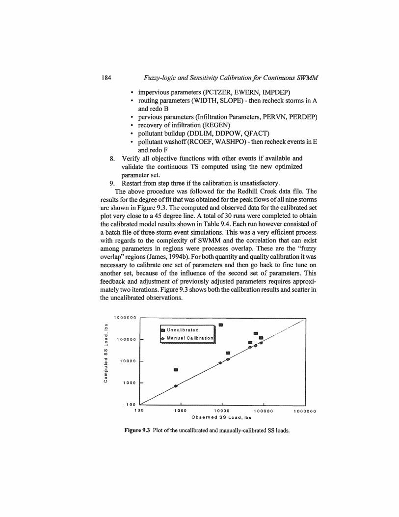
9. Restart from step three if the calibration is unsatisfactory. The above procedure was followed for the Redhill Creek data file. The
results for the degree offit that was obtained for the peak flows of all nine storms are shown in Figure 9.3. The computed and observed data for the calibrated set plot very close to a 45 degree line. A total of 30 runs were completed to obtain the calibrated model results shown in Table 9.4. Each run however consisted of a batch file of three storm event simulations. This was a very efficient process with regards to the complexity of SWMM and the correlation that can exist among parameters in regions were processes overlap. These are the "fuzzy overlap" regions (James, 1994b). For both quantity and quality calibration it was necessary to calibrate one set of parameters and then go back to fine tune on another set, because of the influence of the second set of parameters. This feedback and adjustment of previously adjusted parameters requires approximately two iterations. Figure 9.3 shows both the calibration results and scatter in the uncalibrated observations.
1 000000 r--------------------~
// .. :f!
,--------,. . .., ~ 100000 -'
Uncalibrated
Manual Calibration
'" '" .., .! ::J 0. E o o
10000
• 1000
. 100 ~-----__ ~ _______ ~ ______ ~ _______ ~
100 1000 10000 100000 1000000 Observed 55 Load, Ibs
Figure 9.3 Plot of the uncalibrated and manually-calibrated SS loads.
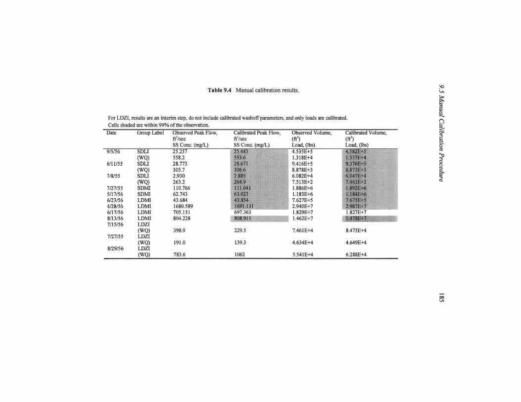
Table 9.4 Manual calibration results.
For LOZI, results are an interim step, do not include calibrated washoffparameters, and only loads are calibrated. Cells shaded are within 99% of the observation.
Date Group Label Observed Peak Flow, Calibrated Peak Flow, Observed Volume, Calibrated Volume,
(WQ) 6111155 SOLI
(WQ) 7/8/55 SOLI
(WQ) 7127/55 SOMI 5/17/56 SOMI 6123/56 LDMI 4128/56 LOMI 6117/56 LOMI 8/13/56 LDMI 7/15156 LOZI
(WQ) 7127/55 LOZI
(WQ) 8129156 LOZI
(WQ)
ftl/sec ft3/sec (ftl) (ftl) SS Cone.
558.2 28.773 305.7 2.930 2632 110.766 62.743 43.684 1680.589 705.151 804.228
398.9 229.5
191.0 139.3
783.6 1062
1.318E+4 9.416E+5 8.878E+3 6.082E+4 7.513E+2 1.886E+6 1.183E+6 7.627E+5 2.940E+7 l.829E+7
II 1.462E+7
7.461E+4
4.634E+4
5.541E+4
" """~ •• i~
8.475E+4
4.649E+4
6288E+4
~ v.
~ ::i
§. ~ :::c;,:. ~ §. ~ ~ ~ ~
-QO VI
186 Fuzzy-logic and Sensitivity Calibration for Continuous SWMM
9.6 Conclusions
Sensitivity analysis tools using a fuzzy logic basis to select appropriate hydro-meteorological inputs are described. A logical calibration proceeds from an understanding of the input parameter space that excites model parameters and their associated processes. Overall complexity of calibration is reduced since only sensitive parameters of active processes are considered ..
The fuzzy logic approach used in this chapter is novel. Selection of event types from the continuous time series was aided by grouping parameters into processes and isolating the regions of input variable space in which each process were dominant. Events similar to those used for the SA were selected from the rainfall TS.
The complexity of calibrating a dataset for the Redhill Creek manually was reduced by grouping parameters with processes that were dominant for specific types of meteorological event. This procedure was efficient, a total of only 90 SWMM runs were required to calibrate fourteen parameter groups to nine quantity and six quality events.
Using sensitivity-based DSS tools for automation of mundane tasks can cut the amount of time required to perform this necessary task by 75% and more. A model calibrated using the steps and software tools outlined in this chapter will be more credible (physically representative and reproduce to a greater extent a range of observations).
Acknowledgments
Tony Kuch did all the hard work and presented it for an MSc degree at the U of Guelph. Bill James collected the resources, and provided the research ideas, guidance, facilities, and support funds through his NSERC research operating grant, and finally wrote this short chapter from Tony's very much longer dissertation. For further information contact Bill James at the U of Guelph.
References
Baffaut, C. and Delleur, J. W., (1989) Expert System for Calibrating SWMM. Journal of Water Resources Planning and Management, ASCE, 115: 279-298.
El-Hossieny, T. (1996) Uncertainty optimization for combined drainage systems. PhD dissertation. U of Guelph, Ontario.
Gregory, M.A. (1995). Management of Time-Series Data for Long-Tenn, Continuous Stonnwater Modelling. Master ofScience (Engineering) Paper University ofGuelph, ·Guelph, Ontario, August 1995.
References 187
Huber, W.C. (1992a). Experience with the U.S. EPA SWMM Model for Analysis and Solution of Urban Drainage Problems. Inundaciones Y Redes de Drenaje Urbano, Dolz J., Gomez, M., and J.P. Martin eds., Colegio de lngenieros de Caminos, Canales y Puertos, May 1992. pp. 199-220.
Huber, W.C.(1992b). PredictionofUrbanNonpointSourceWaterQuality:Methodsand Models. Paper presented at the International Symposium on Urban Stormwater Management, Sydney 4-7 Feb. '92.
Huber, W.C. and Dickinson, R.E. (1988). Storm Water Management Model, Version 4: User's Manuai,Version 4, EPA/600/3-88/00la(NTISPB88-23664ll AAAS),Environmental Protection Agency. Athens, Georgia.
James, W. (1994a). Why design Storm Methods bave become Unethical. In: Hydraulic Engineering '94. Proc. of the National Conference on Hydraulic Engineering, Buffalo, New York, August 1-5, 1994. ASCE. New York, NY (2): 1203-1207.
James, W. (l994b). Rules for Responsible Modelling. Computational Hydraulics International, Guelph, Ontario. 146 pp.
Orlob, G.T. (1992). Water-Quality Modelling for Decision Making. Journal ofWater Resources Planning and Management, ASCE, 11 8: 295-305.
Srikanthan, R. and McMahon, T.A. (1985). Stochastic Generation of Rainfidl and Evaporation Data. Australian Water Resources Council Technical Paper No. 84, 301 pp.
Wang, J.Y. (1996). Integration ofthe US Army Corps ofEngineers Time Series Data Management System with Continuous SWMM Modelling. MSc dissertation, Univ. of Guelph, Guelph, Ontario.
