ARL-TR-9117 ● NOV 2020

Characterization of the High-Speed Detection Limits of a Neuromorphic Vision Sensor by Jonah Sengupta, Ben Linne, and Aaron Bard Approved for public release; distribution is unlimited.

NOTICES

Disclaimers

The findings in this report are not to be construed as an official Department of the Army position unless so designated by other authorized documents.

Citation of manufacturer’s or trade names does not constitute an official endorsement or approval of the use thereof.

Destroy this report when it is no longer needed. Do not return it to the originator.

ARL-TR-9117 ● NOV 2020

Characterization of the High-Speed Detection Limits of a Neuromorphic Vision Sensor Jonah Sengupta Johns Hopkins University Ben Linne and Aaron Bard Weapons and Materials Research Directorate, DEVCOM Army Research Laboratory Approved for public release; distribution is unlimited.

ii

REPORT DOCUMENTATION PAGE Form Approved OMB No. 0704-0188

Public reporting burden for this collection of information is estimated to average 1 hour per response, including the time for reviewing instructions, searching existing data sources, gathering and maintaining the data needed, and completing and reviewing the collection information. Send comments regarding this burden estimate or any other aspect of this collection of information, including suggestions for reducing the burden, to Department of Defense, Washington Headquarters Services, Directorate for Information Operations and Reports (0704-0188), 1215 Jefferson Davis Highway, Suite 1204, Arlington, VA 22202-4302. Respondents should be aware that notwithstanding any other provision of law, no person shall be subject to any penalty for failing to comply with a collection of information if it does not display a currently valid OMB control number. PLEASE DO NOT RETURN YOUR FORM TO THE ABOVE ADDRESS.

1. REPORT DATE (DD-MM-YYYY)

November 2020 2. REPORT TYPE

Technical Report 3. DATES COVERED (From - To)

March–July 2020 4. TITLE AND SUBTITLE

Characterization of the High-Speed Detection Limits of a Neuromorphic Vision Sensor

5a. CONTRACT NUMBER

5b. GRANT NUMBER

5c. PROGRAM ELEMENT NUMBER

6. AUTHOR(S)

Jonah Sengupta, Ben Linne, and Aaron Bard 5d. PROJECT NUMBER

5e. TASK NUMBER

5f. WORK UNIT NUMBER

7. PERFORMING ORGANIZATION NAME(S) AND ADDRESS(ES)

DEVCOM Army Research Laboratory ATTN: FCDD-RLW-PD Aberdeen Proving Ground, MD 21005

8. PERFORMING ORGANIZATION REPORT NUMBER

ARL-TR-9117

9. SPONSORING/MONITORING AGENCY NAME(S) AND ADDRESS(ES)

10. SPONSOR/MONITOR'S ACRONYM(S)

11. SPONSOR/MONITOR'S REPORT NUMBER(S)

12. DISTRIBUTION/AVAILABILITY STATEMENT

Approved for public release; distribution is unlimited.

13. SUPPLEMENTARY NOTES

14. ABSTRACT

Event-based sensors have demonstrated latencies on the scale of 1–10 microseconds, making the technology an energy-efficient, lightweight option for real-time, high-speed object detection and tracking. Research has been conducted to characterize the sensors’ abilities to detect high-speed objects in a controlled environment and establish performance upper limits and induce which on-chip channels and physical mechanisms act as bottlenecks. A configurable LED strip with user interface was designed and implemented to extract this detection cutoff in a lab-controlled environment. Since the event-based sensor responds to changes in intensity, switching on individual LEDs consecutively simulates the effect of an object moving across its field of view. A user interface was embedded into the LED strip to allow for customization of the simulated projectile’s “velocity”. After calibrating the sensor, the detection limit was systematically extracted by increasing this velocity from 50 to 1000 m/s in rough increments. Using a custom signal-processing algorithm, the location of the projectile’s tip was extracted. By tracking the number of average tip positions over the range of recorded shot velocities, linear extrapolation shows the absolute limit of the event-based sensor to be 1450 m/s. Faster speeds and more recordings can be used to verify this conclusion. 15. SUBJECT TERMS

neuromorphic, event based, object detection, characterization, high speed

16. SECURITY CLASSIFICATION OF: 17. LIMITATION OF ABSTRACT

UU

18. NUMBER OF PAGES

22

19a. NAME OF RESPONSIBLE PERSON

Jonah Sengupta a. REPORT

Unclassified b. ABSTRACT

Unclassified

c. THIS PAGE

Unclassified

19b. TELEPHONE NUMBER (Include area code)

(410) 278-6219 Standard Form 298 (Rev. 8/98)

Prescribed by ANSI Std. Z39.18

iii

Contents

List of Figures iv

List of Tables iv

1. Introduction 1

2. Materials, Assumptions, and Procedures 2

2.1 Overview 2

2.2 LED Strip 2

2.3 Neuromorphic Vision Sensor 3

2.4 Basic Testing 6

3. Results and Discussion 6

3.1 Calibration 6

3.2 Data Processing 7

4. Conclusions 13

5. References 14

List of Symbols, Abbreviations, and Acronyms 15

Distribution List 16

iv

List of Figures

Fig. 1 Setup for LED projectile’s acquisition: lower panel’s dimensions are 11.5 × 18.5 inches and NVS is 18 inches above LED strip; LED “projectile” propagates left to right across NVS’s field of view (FOV) and is acquired by NVS, connected via USB 3.0 to laptop .................. 2

Fig. 2 Adafruit Dotstar LED strip with Blue Pill microprocessor on custom protoboard ............................................................................................. 3

Fig. 3 DAVIS346 and 4–12-mm telescopic C-mount lens ............................. 4

Fig. 4 NVS responds to positive changes in the photocurrent by producing ON events and negative changes with OFF events, when the level exceeds global thresholds (specified by dotted lines); after a spike, output returns to a reset level ................................................................ 5

Fig. 5 World to pixel-coordinate transformations ........................................... 7

Fig. 6 Shot-detection outputs with X-axis of each plot as event index: first row—raw event timestamp outputs; second row—derivative of timestamps with respect to index; third row—second difference of timestamps; and fourth row—Boolean variable classifying when a shot has occurred .......................................................................................... 9

Fig. 7 Cropped event stream—timestamps and x-addresses; X-axis is index and Y-axis is event value .................................................................... 10

Fig. 8 Projectile-tip detection output: rolling maximum is depicted with blue points overlaid on event’s x-addresses ............................................... 11

Fig. 9 Number of detected pixels vs. LED projectile velocities; linear, least-squares fit is shown with solid line and its respective equation ......... 12

List of Tables

Table 1 DAVIS346 specifications ..................................................................... 4

Table 2 Important DAVIS346 biases for high-speed applications .................... 5

Table 3 DAVIS346’s intrinsic parameters ......................................................... 7

Table 4 Detection characterization results ....................................................... 12

1

1. Introduction

Despite the advances due to exponential technological growth over the last half century, computers and solid-state devices still lag behind human performance in some key fields. Biological systems consistently outperform computer-aided devices, specifically with regards to perception tasks and fine motor control. Even more impressively, biological entities perform these tasks at factors of increased efficiency due to low energy expenditure in contrast to large computers. Because of this advantage, research into emulation of these biological processes has been a vital approach to implementing energy-efficient sensor platforms. Most prominently, there has been considerable work into the research and commercialization of technology centered on the translation of functionality from the retina into vision chips: neuromorphic vision sensors (NVSs).

Like the retina, these sensors only respond to changes in scenes’ light reflectances and generate bipolar spike responses asynchronously. In this paradigm, the change of light is encoded in the spiking times rather than the absolute intensity, which is the typical output from charge-coupled device (CCD) and complementary metal–oxide–semiconductor (CMOS) image sensors. Information transmission from the NVS greatly improves upon the redundant information read from traditional CMOS image sensors. Assuming a static camera, only moving objects produce spiking responses from the NVS, in contrast to a CMOS camera, which produces millions of bits from the periodic framing regardless of scene dynamics. Information latency, defined as the time between the photonic arrival and output from the chip, is also reduced due to the asynchronous nature of transmission, as each pixel can be attended to by the chip interface independent of its location on the chip. In these ways, NVSs correct the simultaneous oversampling and undersampling issues encountered by traditional machine-vision platforms as redundant background information is neglected and salient events are read out as fast as possible.

NVSs have demonstrated latencies on the scale of 1–10 microseconds, making the technology an energy-efficient, lightweight option for real-time, high-speed object detection and tracking. In the scope of neuromorphic vision research, no complete work has been conducted into characterizing the limits of the NVS’s high-speed detection capabilities. In this technical report such research has begun and its setup and methods will be detailed. The objective of this work is to understand the NVS’s ability to detect high-speed objects in a controlled-environment to establish performance upper limits and induce what on-chip channels and physical mechanisms act as bottlenecks.

2

2. Materials, Assumptions, and Procedures

2.1 Overview

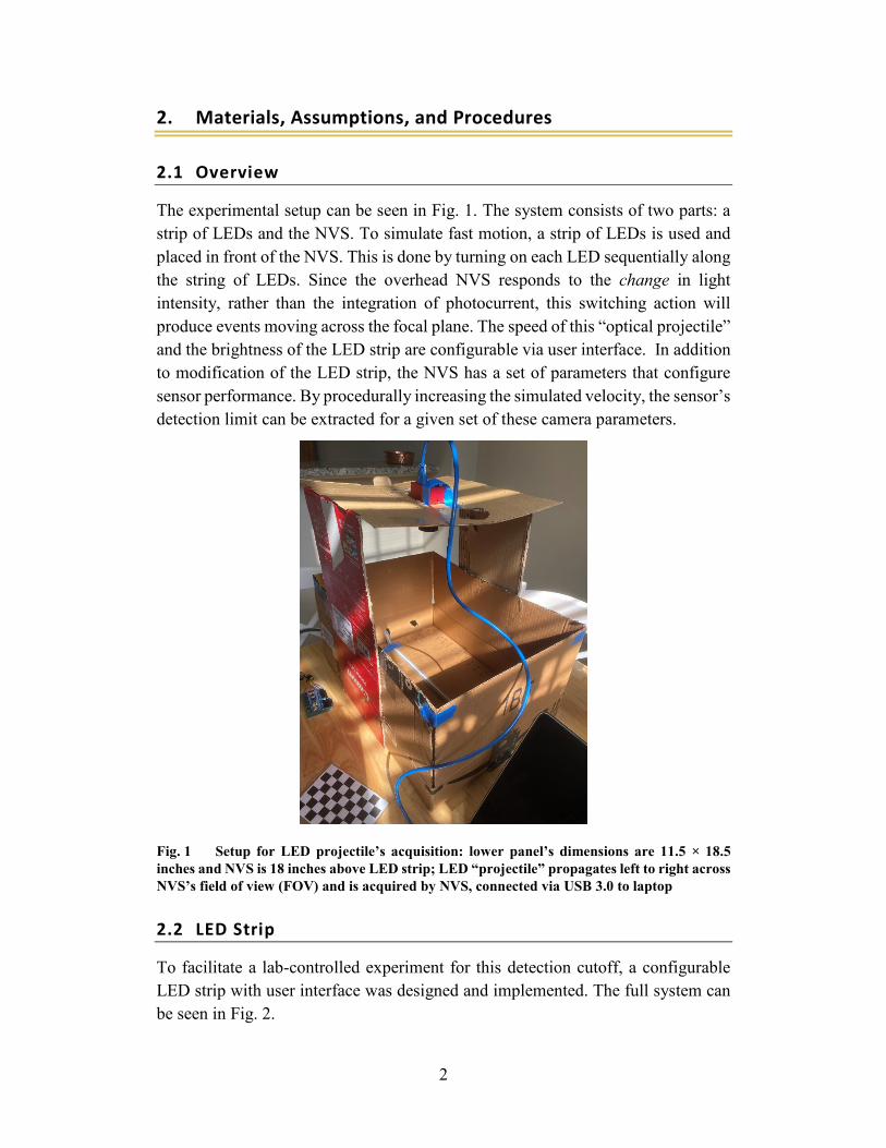
The experimental setup can be seen in Fig. 1. The system consists of two parts: a strip of LEDs and the NVS. To simulate fast motion, a strip of LEDs is used and placed in front of the NVS. This is done by turning on each LED sequentially along the string of LEDs. Since the overhead NVS responds to the change in light intensity, rather than the integration of photocurrent, this switching action will produce events moving across the focal plane. The speed of this “optical projectile” and the brightness of the LED strip are configurable via user interface. In addition to modification of the LED strip, the NVS has a set of parameters that configure sensor performance. By procedurally increasing the simulated velocity, the sensor’s detection limit can be extracted for a given set of these camera parameters.

Fig. 1 Setup for LED projectile’s acquisition: lower panel’s dimensions are 11.5 × 18.5 inches and NVS is 18 inches above LED strip; LED “projectile” propagates left to right across NVS’s field of view (FOV) and is acquired by NVS, connected via USB 3.0 to laptop

2.2 LED Strip

To facilitate a lab-controlled experiment for this detection cutoff, a configurable LED strip with user interface was designed and implemented. The full system can be seen in Fig. 2.

3

Fig. 2 Adafruit Dotstar LED strip with Blue Pill microprocessor on custom protoboard

This full system comprises two components: an Adafruit Dotstar LED strip1 with a STM32 Blue Pill microprocessor2 that controls the strip. The connection to the LED strip is made via a four-wire Serial Peripheral Interface (SPI) that can be operated as fast as the supplied microprocessor. The Blue Pill microprocessor can be operated at 72 MHz and includes 64 KB of flash memory and 20 KB of static random-access memory. In addition to the master microprocessor, there are microcontrollers in every series-connected LED that control brightness, color, and mode of operation (ON or OFF). To simulate a projectile in the horizontal FOV (H-FOV) of the NVS, an ON instruction is sent to each pixel and propagated by the SPI clock serially down the LED strip. Once this has reached the end of the strip, after 1 s, an OFF command is propagated to refresh the strip. By adjusting the SPI clock provided by the Blue Pill, the simulated speed of the optical projectile can be adjusted from 1 to 3846 m/s. The clock’s configuration is set via push buttons on the protoboard that sets increments on the clock at 1, 10, 100, or 1000. For ease of use, an LCD screen was added to the protoboard to display the clock settings and the speed of the optical projectile.

2.3 Neuromorphic Vision Sensor

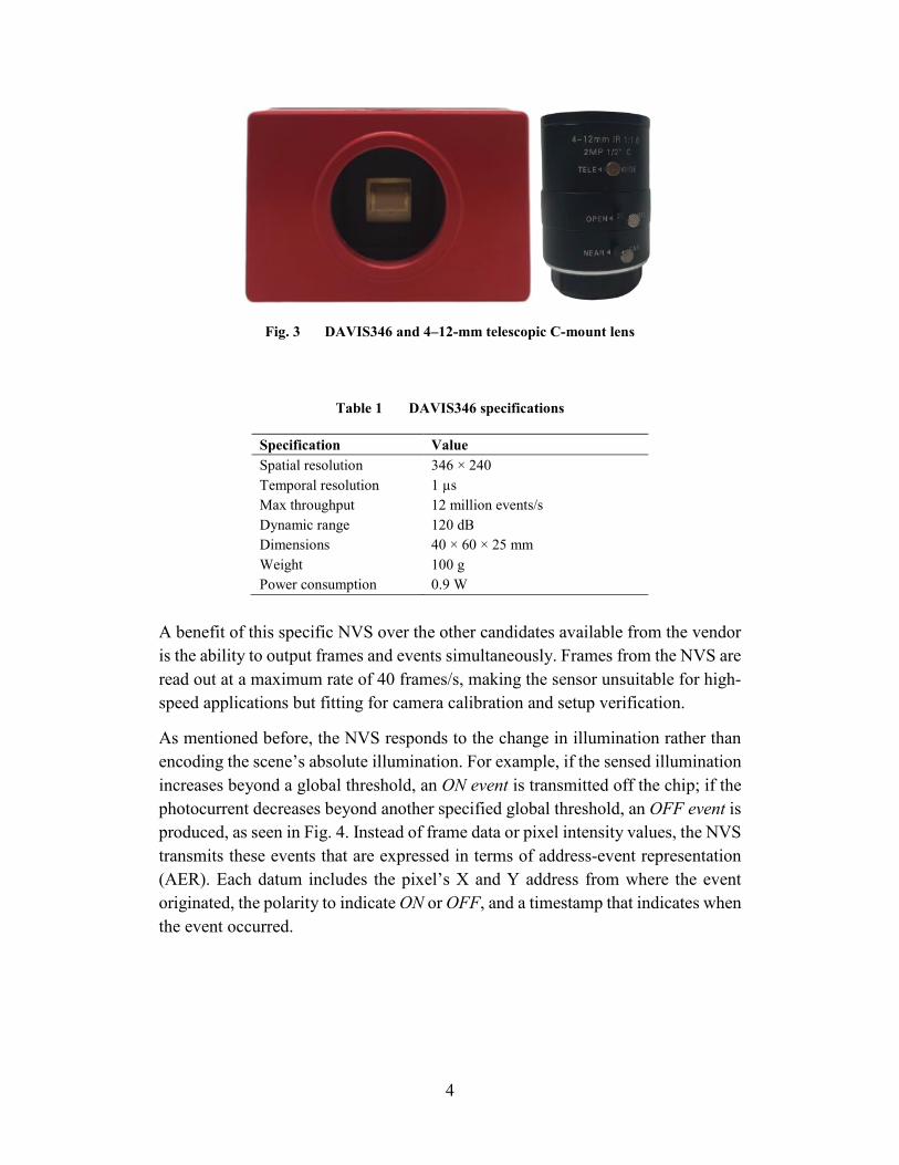
The NVS chosen for this experiment, seen in Fig. 3, was the DAVIS3463 supplied by iniVation AG. The specifications of NVS, extracted from the referenced data sheet, can be found in Table 1.

4

Fig. 3 DAVIS346 and 4–12-mm telescopic C-mount lens

Table 1 DAVIS346 specifications

Specification Value Spatial resolution 346 × 240 Temporal resolution 1 µs Max throughput 12 million events/s Dynamic range 120 dB Dimensions 40 × 60 × 25 mm Weight 100 g Power consumption 0.9 W

A benefit of this specific NVS over the other candidates available from the vendor is the ability to output frames and events simultaneously. Frames from the NVS are read out at a maximum rate of 40 frames/s, making the sensor unsuitable for high-speed applications but fitting for camera calibration and setup verification.

As mentioned before, the NVS responds to the change in illumination rather than encoding the scene’s absolute illumination. For example, if the sensed illumination increases beyond a global threshold, an ON event is transmitted off the chip; if the photocurrent decreases beyond another specified global threshold, an OFF event is produced, as seen in Fig. 4. Instead of frame data or pixel intensity values, the NVS transmits these events that are expressed in terms of address-event representation (AER). Each datum includes the pixel’s X and Y address from where the event originated, the polarity to indicate ON or OFF, and a timestamp that indicates when the event occurred.

5

`

Fig. 4 NVS responds to positive changes in the photocurrent by producing ON events and negative changes with OFF events, when the level exceeds global thresholds (specified by dotted lines); after a spike, output returns to a reset level

The NVS’s ability to detect these changes with respect to signal amplitude and frequency is determined by a set of circuit voltages or analog biases. These six voltages can be configured via the Dynamic Vision (DV) platform used to interface with the DAVIS346. Of these six parameters, four are relevant to the operation of the pixel for high-speed applications. These are described and listed in Table 2.

Table 2 Important DAVIS346 biases for high-speed applications

Parameter Description Photoreceptor bias (PrBp) Controls the pixels’ bandwidth, assuming adequate background

illumination; if the value is high, the pixel can detect fast frequencies but also will respond to high-frequency noise.

Differential (DiffBn) Similar to the photoreceptor bias; controls the speed of an amplifier element and sets the reset level of the pixel.

On threshold (OnBn) Sets the ON threshold in the pixel (i.e., the level above the reset voltage where an ON event is transmitted); higher value makes the pixel less sensitive to positive changes.

Off threshold (OffBn) Sets the OFF threshold in the pixel (i.e., the level above the reset voltage where an OFF event is transmitted); higher value makes the pixel less sensitive to negative changes.

6

For this set of experiments, the default parameters provided in the DV platform were used. This set is optimal for general use and provides a baseline with which further research can be compared for this NVS.

2.4 Basic Testing

The systematic extraction of a maximum detection capability of the NVS was done by coarsely incrementing the optical projectile’s velocity and running a signal-processing algorithm to determine the number of activated pixels. Since the NVS can simultaneously output frames and events, the frames are used to calibrate the sensor and extract its intrinsic parameters. The streams were corrected for lens distortions using these camera parameters and seven recordings. To coarsely estimate this maximum detection velocity, seven speeds were chosen: 50, 100, 200, 350, 500, 750, and 1000 m/s. Each capture is 6 s long and includes three full ON–OFF LED sequences. Background illumination had to be increased in order to ensure the LED brightness did not saturate the camera and that each LED pixel could be spatially correlated in the NVS recording (meaning there was not a light bloom radiating outward from the strip).

3. Results and Discussion

3.1 Calibration

In most machine-vision experiments and applications, camera calibration, or the process to extract the camera’s intrinsic and extrinsic parameters, is the typical first step. For traditional computer vision there are well-established procedures in MATLAB and OpenCV that allow for proper calibration. However, the NVS domain lacks well-established processes due to the nature of the sensor. Since the DAVIS346 has the ability to output frames in parallel, the sensor can be calibrated in a typical manner. By presenting a well-defined checkerboard pattern and allowing the calibration module within DV to capture images using the NVS, calibration error can be minimized and the camera parameters can be produced. The DV platform that was used to capture the NVS output can also be used to calibrate the sensor in real time.

Using the intrinsic camera parameters and the measurements of the setup, the dimensions of a single LED within the strip can be extracted. From the product data sheet, the LED’s lateral dimension is x = 5 mm. As seen in Fig. 1, the sensor is displaced z = 18.25 inches or 463.55 mm from the LED strip. Assuming a simple pinhole model of the camera and neglecting lens distortion, the pixel coordinates

7

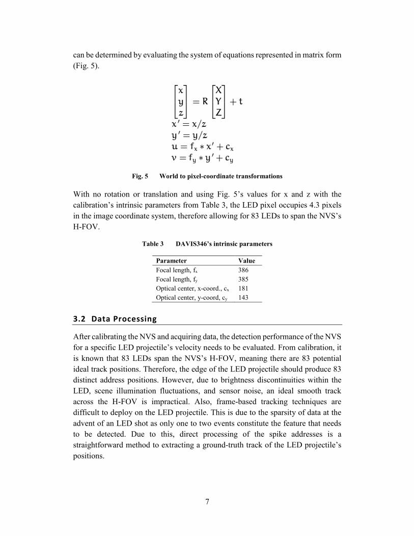
can be determined by evaluating the system of equations represented in matrix form (Fig. 5).

Fig. 5 World to pixel-coordinate transformations

With no rotation or translation and using Fig. 5’s values for x and z with the calibration’s intrinsic parameters from Table 3, the LED pixel occupies 4.3 pixels in the image coordinate system, therefore allowing for 83 LEDs to span the NVS’s H-FOV.

Table 3 DAVIS346’s intrinsic parameters

Parameter Value Focal length, fx 386 Focal length, fy 385 Optical center, x-coord., cx 181 Optical center, y-coord, cy 143

3.2 Data Processing

After calibrating the NVS and acquiring data, the detection performance of the NVS for a specific LED projectile’s velocity needs to be evaluated. From calibration, it is known that 83 LEDs span the NVS’s H-FOV, meaning there are 83 potential ideal track positions. Therefore, the edge of the LED projectile should produce 83 distinct address positions. However, due to brightness discontinuities within the LED, scene illumination fluctuations, and sensor noise, an ideal smooth track across the H-FOV is impractical. Also, frame-based tracking techniques are difficult to deploy on the LED projectile. This is due to the sparsity of data at the advent of an LED shot as only one to two events constitute the feature that needs to be detected. Due to this, direct processing of the spike addresses is a straightforward method to extracting a ground-truth track of the LED projectile’s positions.

8

The first step in processing the event stream is detecting the LED projectile occurrences or “shots”. An example of the output from this step is seen in Fig. 6. Raw timestamps from the event stream can be seen on the first row of Fig. 6. This step waveform is a result of the LED shots: When the LED projectile travels through the H-FOV, a large density of pixels produce ON events while the interval between shots yields only noise events since the scene is static. Because of this difference between event densities in the presence of a shot, the derivative of this wave form is taken. To filter out high-frequency noise, a second derivative is taken once again. This value is transformed into a binary variable using a manual threshold where a 1 indicates small derivatives and vice-versa for a 0 state. A sequence of consecutive 1’s or second-derivative values of consequence indicates the presence of a shot, whose waveform is seen in the fourth row of Fig. 6. Using the prior states of this signal, rising and falling edges can be extracted and the shot durations and advents can be found. Difficulty of distinguishing shots arises due to the turn-off sequences of the LED strip since the NVS perceives a large influx of events when the strip deactivates. Since a shot involves a large increase in scene illuminance, the event stream should be entirely composed of ON events. Hence, the percentage of ON events was also considered and used to differentiate between shots and turn-off events.

9

Fig. 6 Shot-detection outputs with X-axis of each plot as event index: first row—raw event timestamp outputs; second row—derivative of timestamps with respect to index; third row—second difference of timestamps; and fourth row—Boolean variable classifying when a shot has occurred

10

Using the acquired shot times, the event stream is trimmed and the x-address is analyzed around the shot occurrence. A cropped x-address and timestamp stream can be seen in Fig. 7. As can be seen from the figure, there are substantial oscillations present in the x-address stream. This is due to the readout scheme used to transfer the events from the sensor, which attends to the fired event in a row-by-row fashion.

Fig. 7 Cropped event stream—timestamps and x-addresses; X-axis is index and Y-axis is event value

However, despite the presence of these oscillations, the average x-addresses are increasing as a function of event index until the projectile is fully through the H-FOV. To quantify this, the rolling maximum of the x-address stream was determined and can be seen in Fig. 8 as the blue curve. It is known a priori that the projectile is moving in the positive x direction; hence, the tip would correlate to the maximum x-address. This algorithm steps through the stream sequentially and finds the maximum x-address until it encounters the edge of the pixel array. These values are depicted with the blue points in Fig. 8. To quantify the tracking, the number of unique x-coordinates in these maximum values are found and compared with the theoretical limit of 83. This is repeated for each acquired velocity and averaged over every shot in the recording, and the results are seen in Table 4. The table shows the number of detected points from the algorithm are greater than the theoretical limit of 83. This can be attributed to the fact the LED itself is not of uniform texture

11

so when the device turns on, multiple events can be activated. In addition, it should be noted that the LED is driven by a pulse-width modulated signal. Ideally, the LEDs should be driven by a DC voltage when programmed to emit maximum brightness. If the driving voltage is fluctuating during the turn-on state, the amount of events detected by the sensor will vary in accordance. This fact can be pondered on further as the algorithm is developed.

Fig. 8 Projectile-tip detection output: rolling maximum is depicted with blue points overlaid on event’s x-addresses

Figure 9 contains a plot of detected points versus projectile velocity. It can be seen there is a nearly inverse linear relation between detections and LED projectile velocities. Fitting a first-order function to the data yields a line with a slope of –0.08 detections (per m/s). With this fit, the limit for 0 detections is a projectile with a velocity of 1472 m/s.

12

Fig. 9 Number of detected pixels vs. LED projectile velocities; linear, least-squares fit is shown with solid line and its respective equation

The second column of Table 4 is the calculated optical flow, the speed of the projectile on the image sensor plane, using the calibration results and the derived LED projectile’s velocity. From the DAVIS346 data sheet it is known the time resolution of the sensor is 1 µs, so the optical flow is presented in terms of this unit. When the sensor reaches this resolution limit, the timestamps are identical. For this experimental setup, the absolute theoretical limit can be seen to be 5000 m/s as that corresponds to 4.2 pix/µs, which matches the pixel dimensions of a LED. However, due to sensor noise and other non-ideal behavior, this value could be much lower and is a subject of future study.

Table 4 Detection characterization results

Velocity (m/s)

Optical flow (pix/µs)

Detected x-address (no. of pix)

50 0.042 131.3 100 0.084 113.6 250 0.210 85 350 0.294 79.5 500 0.420 77.0 750 0.630 54.7

1000 0.840 47.3

13

4. Conclusions

A preliminary velocity-detection limit was extracted for the commercial off-the-shelf NVS, the DAVIS346. Using a user-configurable LED strip that simulates high-speed projectiles, a series of recordings of “shots” were systematically captured and used to characterize the NVS. A maximum velocity of 1472 m/s was extrapolated by linearly fitting the detected positions of this optical projectile. This is a first effort in the characterization of these event-based sensors which, depending on the results and confirmation of further research, provide low-cost, energy and space-efficient solution to detect and track high-speed threats.

There are two possible efforts to advance future investigation into the NVS’s limit of high-speed detection capabilities: testing advancements and algorithm development. The first effort involves changing the testing procedure. For example, another NVS can be used to capture the LED projectile data. Readout latency and speed for NVSs is partially a function of sensor resolution, so understanding the relationship between object detection and sensor size is important to realize with the LED projectile. Second, the NVS can be reconfigured with a different set of camera biases. As stated in the Section 2, these parameters greatly influence sensor performance with regard to latency and pixel bandwidth. By adjusting the parameters to “speed” up the pixel, an absolute limit can be found for the NVS while also considering the signal-to-noise ratio of the sensor (increasing pixel bandwidth comes with the cost of increasing the noise factor). Another future step in testing involves acquiring data based on other LED velocities. First, the range of acquired velocities can be extended past the current maximum of 1000 m/s. Secondly, additional velocities can be captured to populate the intervals of the current experiment. The former improvement will investigate what the absolute detection limit is for a certain NVS and the latter will add resolution to the detection response of the sensor.

As described in the Section 3, the goal for algorithm development is to characterize the NVS’s detection capabilities. To improve upon current results, the current algorithm flow should be repeated over a large amount of samples of the same velocity in order to generalize the NVS’s functionality for a certain speed. Due to sensor noise or scene fluctuations, event acquisition for the same projectile can vary to the point where a large amount of data is needed to average out these discrepancies. In addition to running on a larger data set, the algorithm itself will be improved. At present, the algorithm is manually configured for each event stream in order to extract the top of the LED projectile. By using a Kalman filter, which incorporates a model of the position noise and a fixed estimate of the LED velocity, a filtered event position can be extracted. By comparing this estimate with the same noise model, detection performance for each velocity can be evaluated.

14

5. References

1. Burgess P. Adafruit DotStar LEDs. Adafruit Industries; c2020 [accessed 2020 Sep 29]. https://cdn-learn.adafruit.com/downloads/pdf/adafruit-dotstar-leds.pdf?timestamp=1597357594.

2. Medium-density performance line ARM®-based 32-bit MCU with 64 or 128 KB flash, USB, CAN, 7 timers, 2 ADCs, 9 com. interfaces. STMicroelectronics; c2015 [accessed 2020 Sep 29]. https://www.st.com/resource/en/datasheet/stm32f103c8.pdf.

3. Specifications—current models. Zurich (Switzerland): iniVation AG; c2020 [accessed 2020 Sep 29]. https://inivation.com/wp-content/uploads/ 2020/06/2020-05-11-DVS-Specifications.pdf.

15

List of Symbols, Abbreviations, and Acronyms

AER address-event representation

ARL Army Research Laboratory

CCD charge-coupled device

CMOS complementary metal–oxide–semiconductor

DC direct current

DEVCOM US Army Combat Capabilities Development Command

DV Dynamic Vision

FOV field of view

H-FOV horizontal field of view

LCD liquid-crystal display

LED light-emitting diode

NVS neuromorphic vision sensor

SPI Serial Peripheral Interface

USB Universal Serial Bus

16

1 DEFENSE TECHNICAL (PDF) INFORMATION CTR DTIC OCA 1 DEVCOM ARL (PDF) FCDD RLD DCI TECH LIB 3 DEVCOM ARL (PDF) FCDD RLW PD J SENGUPTA B LINNE A BARD