ClassificationAlgorithmsinApacheSystemML

PrithvirajSen

Overview

• SupervisedLearningandClassification• TrainingDiscriminativeClassifiers• Representer Theorem• SupportVectorMachines• LogisticRegression• GenerativeClassifiers:NaïveBayes• DeepLearning• TreeEnsembles

ClassificationandSupervisedLearning

• Supervisedlearningisamajorareaofmachinelearning• Goalistolearnfunction𝑓 suchthat:

𝑓:ℝm →Cwhere:misafixedinteger

Cisafixeddomainoflabels• Training:goalistolearn𝑓 fromalabeled dataset• Testing:goalistoapply𝑓 tounseenx∈ ℝm

• Applications:• spamdetection(D={spam,no-spam})• searchadvertising(eachadisalabel)• recognizinghand-writtendigits(D={0,1,…,9})

TrainingaClassifier

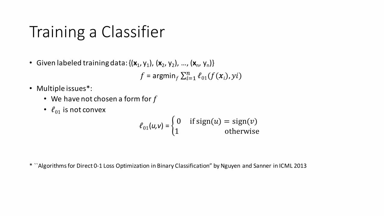
• Givenlabeledtrainingdata:{(x1,y1),(x2,y2),…,(xn,yn)}𝑓=argmin𝑓 ∑ ℓ01(𝑓(𝒙𝑖), 𝑦𝑖)/

012

• Multipleissues*:• Wehavenotchosenaformfor𝑓• ℓ01 isnotconvex

ℓ01(u,v)=30ifsign(𝑢) = sign(𝑣)1otherwise

*``AlgorithmsforDirect0-1LossOptimizationinBinaryClassification”byNguyenandSanner inICML2013

TrainingDiscriminativeClassifiers

𝑓=argmin𝑓 ∑ ℓ(𝑓(𝒙𝑖), 𝑦𝑖)+ℊ(∥ 𝑓 ∥)/012

• Thesecondtermis``regularization”• Acommonformfor𝑓(𝒙) is𝐰′𝒙 (linearclassifier)• ℓ(w’x,y)is``convexified”loss• Besidesdiscriminativeclassifiers,generativeclassifiersalsoexist

• e.g.,naïveBayes

Classifier Lossfunction(y∈ {±1})supportvectormachine max(0,1- yw’x)logisticregression log[1+exp(-yw’x)]adaboost exp(-yw’x)square loss (1– yw’x)2

Algorithms for Direct 0–1 Loss Optimization in Binary Classification

−1.5 −1 −0.5 0 0.5 1 1.5 20

1

2

3

4

5

6

7

8

margin (m)

Loss

Valu

e

0−1 LossHinge LossLog LossSquared Loss

Figure 2. Di↵erent losses as a function of the margin.

search through combinations of data points that definethese equivalence classes. While systematic combina-torial search yields e�cient optimal solutions on lowdimensional problems, heuristic combinatorial searcho↵ers excellent approximations and scalability.

Smooth, di↵erentiable relaxations of 0–1 loss: We re-lax the 0–1 loss to a smooth, di↵erentiable functionthat can arbitrarily approximate the original 0–1 lossvia a smoothness constant. We then provide an itera-tively unrelaxed coordinate descent approach for gra-dient optimization of this smoothed loss along withtechniques for escaping local optima. This yields solu-tions comparable to the combinatorial search approxi-mation, while running two orders of magnitude faster.

Empirically, we compare our proposed algorithms tologistic regression, SVM, and the Bayes point machine(a approximate Bayesian approach with connectionsto the 0–1 loss) showing that the proposed 0–1 lossoptimization algorithms perform at least comparablyand o↵er a clear advantage in the presence of outliers.

2. Linear Binary Classification

We assume a D-dimensional data input vector x 2 RD

(D for dimension), where the goal of binary classifica-tion is to predict the target class t 2 {�1, 1} for agiven x. Linear binary classification which underliesmany popular classification approaches such as SVMsand logistic regression defines a predictor function:

fw

(x) =DX

j=1

wjxj + w0 = w

Tx+ w0, (1)

where wj 2 R and w0 2 R is a bias. Then

t =

(1 f

w

(x) � 0

�1 fw

(x) < 0(2)

Thus, the equation of the decision boundary that sep-arates the two classes is f

w

(x) = w

Tx+w0 = 0, which

is a D-dimensional hyperplane.

We use two notations for the weight vector w:in the homogeneous notation, we assume w =(w0, w1, . . . , wD)T and x = (1, x1, . . . , xD) so thatfw

(x) = w

Tx. In the non-homogeneous notation, we

assume w = (w1, . . . , wD)T and x = (x1, . . . , xD) sothat f

w

(x) = w

Tx+ w0.

The training dataset contains N data vectors X ={x1,x2, . . . ,xN} and their corresponding target classt = {t1, t2, . . . , tN}. To measure the confidence of aclass prediction for an observation xi 2 X, the so–called margin is defined as mi(w) = tifw(xi). Amargin mi(w) < 0 indicates xi is misclassified, whilemi(w) � 0 indicates xi is correctly classified and mi

represents the “margin of safety” by which the predic-tion for xi is correct (McAllester, 2007).

The learning objective in classification is to find thebest (homogenous) w to minimize some loss over thetraining data (X, t), i.e.,

w

⇤ = argminw

NX

i=1

L(mi(w)) + �R(w), (3)

where loss L(mi(w)) is defined as a function of themargin for each data point xi, R(w) is a regularizerwhich prevents overfitting (typically kwk22 or kwk1),and � > 0 is the regularization strength parameter.

Some popular losses as a function of the margin are

0–1 loss: L01(mi

(w)) = I[mi

(w) 0], (4)

squared loss: L2(mi

(w)) =1

2[m

i

(w)� 1]2 (5)

hinge loss: Lhinge

(mi

(w)) = max(0, 1�m

i

(w)) (6)

log loss: L

log

(mi

(w)) = ln(1 + e

�mi(w)) (7)

where I[·] is the indicator function taking the value1 when its argument is true and 0 when false. Theselosses are plotted in Figure 2. 0–1 loss is robust to out-liers since it is not a↵ected by a misclassified point’sdistance from the margin, but this property also makesit non-convex; the convex squared, hinge, and loglosses are not robust to outliers in this way since theirpenalty does scale with the margin of misclassification.Squared loss is not an ideal loss for classification sinceit harshly penalizes a classifier for correct margin pre-dictions � 1, unlike the other losses. This leaves uswith hinge loss as optimized in the SVM and log lossas optimized in logistic regression as two convex sur-rogates of 0–1 loss for later empirical comparison.

Representer Theorem*

• Ifℊ isreal-valued,monotonicallyincreasingandliesin[0,∞)• Andifℓ liesinℝ⋃{∞},then

f(x) =∑ 𝛼𝑖𝒙′𝒙𝑖/012

• Inparticular,• Neitherconvexitynordifferentiabilityisnecessary• Buthelpswiththeoptimization• Especiallywhenusinggradientbasedmethods

*``AGeneralizedRepresenter Theorem”byScholkopf, Herbrich andSmola inCOLT2001☨``WhenisthereaRepresenter Theorem?”byArgyriou,Micchelli andPontil inJMLR2009

BinaryClassSupportVectorMachines

minw∑ max 0, 1 − 𝑦𝑖𝒘S𝒙𝑖 +TU𝒘

S𝒘/012

• Expressedinstandardform:

minw∑ ξi+TU𝒘

S𝒘0

s.t. 𝑦𝑖𝒘S𝒙𝑖 ≥ 1 − ξi∀𝑖ξi ≥ 0∀𝑖

• Lagrangian (𝛼𝑖, 𝛽𝑖 ≥ 0):

ℒ = ∑ ξi+TU𝒘

S𝒘+ ∑ 𝛼𝑖(1 − 𝑦𝑖𝒘S𝒙𝑖 − ξi00 ) − ∑ 𝛽𝑖𝜉𝑖0]ℒ𝝏w:w =2_∑ 𝛼𝑖𝑦𝑖𝒙𝑖0]ℒ𝝏`i:1=𝛼𝑖+𝛽𝑖∀𝑖

BinarySVM:DualFormulation

max𝛼 ∑ 𝛼𝑖0 − 2U∑ 𝛼𝑖𝛼𝑗𝑦𝑖𝑦𝑗𝒙𝑖′𝒙𝑗0b

s.t. 0 ≤ 𝛼𝑖 ≤ 1∀𝑖• ConvexQuadraticProgram• OptimizationalgorithmssuchasPlatt’sSMO*exist• Alsopossibletooptimizetheprimaldirectly(l2-svm.dml,nextslide)• Kerneltrick:

• RedefineinnerproductK(xi,xj)• Projectsdataintoaspace𝜙(𝒙) whereclassesmaybeseparable• Wellknownkernels:radialbasisfunctions,polynomialkernel

*``SequentialMinimalOptimization:AFastAlgorithmforTrainingSupportVectorMachines”byPlatt,TechReport1998.

BinarySVMinDML

minw𝜆𝒘S𝒘+ ∑ max2 0, 1 − 𝑦𝑖𝒘S𝒙𝑖 /012

• Solvefor𝒘 directlyusing:• Nonlinearconjugategradientdescent• Newton’smethodtodeterminestepsize

• Mostcomplexoperationinthescript• Matrix-vectorproduct• Incrementalmaintenence usingvector-vector

operations

Matrix-vectorproduct

Matrix-vectorproduct

Fletcher-Reeves formula

1DNewtonmethodtodeterminestepsize

Multi-ClassSVMinDML

• Atleast3differentwaystodefinemulti-classSVMs• One-against-the-rest* (OvA)• Pairwise (orone-against-one)• Crammer-SingerSVM☨

• OvA multi-classSVM• EachbinaryclassSVMlearntinparallel• Innerbodyuses l2-svm’sapproach

*``InDefenseofOne-vs-All Classification” byRifkinandKlautau inJMLR2004

☨``OntheAlgorithmicImplementationofMulticlassKernel-BasedVectorMachines”byCrammerandSingerinJMLR2002

…

Parallelforloop

LogisticRegressionmaxw -∑ log 1 + 𝑒hi0𝒘j𝒙0 −TU𝒘

S𝒘/012

• Toderivethedualformusethefollowingbound*:log 2

2klmn𝒘j𝒙≤ min𝛼𝛼𝑦𝒘′𝒙 − 𝐻(𝛼)

where0 ≤ 𝛼 ≤ 1 and𝐻(𝛼)=−𝛼log(𝛼) − (1 − 𝛼)log(1 − 𝛼)

• Substituting:maxwmin𝛼 ∑ 𝛼𝑖𝑦𝑖𝒘′𝒙𝑖0 − 𝐻(𝛼𝑖)−

TU𝒘

S𝒘s.t. 0 ≤ 𝛼𝑖 ≤ 1∀𝑖]ℒ𝝏w:w =2_∑ 𝛼𝑖𝑦𝑖𝒙𝑖0

• Dualform:min𝛼

2UT∑ 𝛼𝑖𝛼𝑗𝑦𝑖𝑦𝑗𝒙𝑖′𝒙𝑗0b − ∑ 𝐻(𝛼𝑖)0 s.t.0 ≤ 𝛼𝑖 ≤ 1∀𝑖

• Applykerneltricktoobtainkernelized logisticregression

*``ProbabilisticKernelRegressionModels”byJaakkola andHausslerinAISTATS1999

MulticlassLogisticRegression

• Alsocalledsoftmax regressionormultinomiallogisticregression• Wisnowamatrixofweights,jth columncontainsthejth class’sweights

Pr(y|x)= lpjqn

∑ lpjqnn

minW_U ∥ 𝑊 ∥ 2 + ∑ [log(Zi)0 − 𝑥𝑖′𝑊𝑦𝑖]where𝑍𝑖 = 1S𝑒wjx0

• TheDMLscriptiscalledMultiLogReg.dml• Usestrust-regionNewtonmethodtolearntheweights*• Careneedstobetakenbecausesoftmax isanover-parameterizedfunction

*Seeregressionclass’s slides onibm.biz/AlmadenML

GenerativeClassifiers:NaïveBayes

• Generativemodels“explain”thegenerationofthedata• NaïveBayesassumes,eachfeatureisindependentgivenclasslabel

Pr(x,y)=py∏ (𝑝𝑦𝑗b )nj

• A conjugatepriorisusedtoavoid0probabilities

Pr({(xi,yi)})=∏ [ {|(_)

{(|_)∏ 𝑝𝑦𝑗 𝜆]bi ∏ [𝑝𝑦𝑖∏ 𝑝𝑦𝑖𝑗 𝑛𝑖𝑗]b0

s.t. 𝑝𝑦∀𝑦, 𝑝𝑦𝑗∀𝑦∀𝑗 formlegaldistributions• Maximumisobtainedwhen:

𝑝𝑦 = 𝑛𝑦

∑ 𝑛𝑦i∀𝑦, 𝑝𝑦𝑗 =

𝜆 +∑ 𝑛𝑖𝑗0:i01i𝑚𝜆 + ∑ ∑ 𝑛𝑖𝑗b0:i01i

∀𝑦∀𝑗

• Thisismultinomial naïveBayes,otherformsincludemultivariateBernoulli*

*``AComparisonofEventModels forNaïveBayesTextClassification” byMcCallumandNigaminAAAI/ICML-98Workshop onLearning forTextCategorization

NaïveBayesinDML

• Usesgroupbyaggregates• Veryefficient• Non-iterative• E.g.,documentclassificationwithtermfrequencyfeaturevectors(bag-of-words)

GroupbyaggregateMatrix-vectorop

Groupbycount

DeepLearning:Autoencoders

• Designedtodiscoverthehiddensubspaceinwhichthedata `lives”

• Layer-wisepretraininghelps*• Manyofthesecanbestackedtogether• Finallayerisusuallysoftmax (forclassification)• Weightsmaybetiedornot,outputlayermayhaveanon-linearactivationfunctionornot,manyoptions☨

* ``Afastlearningalgorithmfordeepbeliefnets”byHinton,OsinderoandTeh inNeuralComputation2006

☨ ``OnOptimizationMethodsforDeepLearning”byV.LeetalinICML2011

…

…

…

Inputlayer

Output layer

Hidden layer

DeepLearning:ConvolutionalNeuralNetworks*

• Designedtoexploitspatialandtemporalsymmetry• Akernelisafeaturewhoseweightsarelearnable• Thesamekernelisusedonallpatcheswithinanimage• SystemML surfacesvariousfunctionsandalsomodulestoeaseimplementationofCNNs

• Builtin functions:conv2d,max_pool,conv2d_backward_data,conv2d_backward_filter,max_pool_backward

Convolution with1kernel

Fig. 1. Diagram of LeNet-5 architecture with hyperbolic tangent output layer. Convolutional layer feature maps are indexed by C1, C3, C5. Subsamplinglayer feature maps are indexed S2 and S4.

Fig. 2. Each row from top to bottom. Samples from the mnist-basic,mnist-background-image, mnist-background-rand, mnist-background-image-

rot, mnist-rot dataset, respectively.

Secondly, network weights are randomly initialized from theuniform distribution U(�x, x) following the formula

wk ⇠ U(�v

fe,v

fe) (2)

where f is referred to as the ‘fan-in’ and denotes the numberof incoming connections to a particular feature in a featuremap. The exponent e and numerator v are randomly initializedfrom the uniform distribution with user-set boundaries. Thearchitectures are initialized to be fully-connected (topologymatrices with all entries set to ‘1’).

Each candidate network is trained using backpropagationwith SDLM as a second order method. We chose to use

Fig. 3. Top. Examples from the rectangles-image dataset. Bottom. Examplesfrom the convex dataset.

Fig. 4. Block diagram of architecture evolution process.

SDLM based on the results of Lecun et al. [14], as describedin Section III-B The network is trained on a subset of theprovided training set. This set will be referred to as thetraining-training set. The remaining training examples areused as a validation set, referred to as the training-validation

set. After each generation, the training-training set is swapped

*``Gradient-basedLearningApplied toDocumentRecognition”byLeCun etalinProceedings oftheIEEE,1998

DecisionTree(Classification)

• Simpleandeasytounderstandmodelforclassification• Moreinterpretableresultsthanotherclassifiers• Recursivelypartitionstrainingdatauntilexamplesineachpartitionbelongtooneclassorpartitionbecomessmallenough

• Splittingtests forchoosingfeaturej(xj:jth featurevalueofx)• Numerical:xj <𝜎• Categorical:xj∈ SwhereS ⊆ Domainoffeaturej

• Measuringnodeimpurity𝒥:• Entropy:∑ −𝑓𝑖log(𝑓𝑖)0• Gini:∑ 𝑓𝑖(1 − 𝑓𝑖)0

• Tofindthebestsplitacrossfeaturesuseinformationgain:argmax𝒥 𝑋 −/�l��

/ 𝒥 𝑋𝑙𝑒𝑓𝑡 − /�0���

/ 𝒥 𝑋𝑟𝑖𝑔ℎ𝑡

DecisionTreeinDML

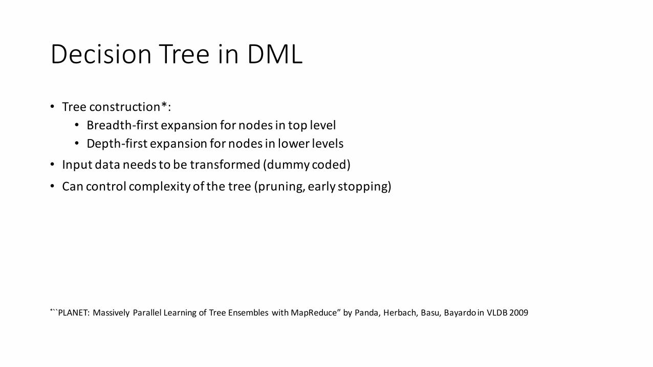
• Treeconstruction*:• Breadth-firstexpansionfornodesintoplevel• Depth-firstexpansionfornodesinlowerlevels

• Inputdataneedstobetransformed(dummycoded)• Cancontrolcomplexityofthetree(pruning,earlystopping)

*``PLANET:Massively ParallelLearningofTreeEnsembleswithMapReduce”byPanda,Herbach,Basu,Bayardo inVLDB2009

RandomForest(Classification)

• Ensembleoftrees• Eachtreeislearntfromabootstrappedtrainingsetsampledwithreplacement• Ateachnode,wesampleforarandomsubsetoffeaturestochoosefrom• Predictionisbymajorityvoting• Inthescript,wesampleusingPoissondistribution• Bydefault,eachtreeis:

• Trainedusing2/3trainingdata• Testedontheremaining1/3(out-of-bagerrorestimation)