co-dominance and succession in temperate forests: a...
TRANSCRIPT
Universita degli Studi della Tuscia di Viterbo
Facolta di Agraria
Dipartimento di
Scienze dell’Ambiente Forestale e delle sue Risorse
(DISAFRI)
Corso di Dottorato di Ricerca in
ECOLOGIA FORESTALE – XXII Ciclo
Co-dominance and Succession in TemperateForests: a Mathematical Approach
settore scientifico disciplinare BIO/07
Coordinatore:
Prof. Paolo De Angelis
Tutor: Dottorando:
Prof. Giuseppe Scarascia Mugnozza Mario Cammarano

ii

iii
Acknowledgements
The work for this thesis has been funded by the European project CIRCE:
Climate Change and Impact Research: the Mediterranean Environment (con-
tract num. 036961). I would like to thank my supervisor Professor Giuseppe
Scarascia Mugnozza and Dr. Giorgio Matteucci for giving me the opportun-
ity to carry out this research at the Istituto di Biologia AgroAmbientale e
Forestale (IBAF) in Rome. At IBAF, I also thank my colleagues and friends
for having contributed to a nice and collaborative environment. I would also
like to thank Prof. Antonello Provenzale and Dr. Mara Baudena at the
Institute ISAC of Torino for stimulating discussions and valuable advices. I
thank Dr. Heike Lischke at WSL in Zurich for her nice hospitality and in-
teresting discussion about forest modelling. I thank my mother, brother and
friends for their support. This thesis would have been tortuous and illegible
without the invaluable help and support of Dr. Ana Rey.
Roma, 7 February 2010

iv
v
Abstract
Forest vegetation covers about one-third of the Earth’s land surface. At
the population level, forests have been widely studied through complex simu-
lators that successfully reproduce observed patterns of long-term successions.
At ecosystem level, while it is well-known that terrestrial ecosystems have po-
tentially large effects on global climate, it is clear that uncertainties in model
predictions are large as well. Such uncertainties could be reduced by incor-
porating in large scale models the ecological realities of biodiversity and com-
petition for light. As vegetation simulators are too complex to run at large
scale, this requires a simpler description of vegetation dynamics. Moreover,
several basic mechanisms of forest dynamics, such as the co-dominance of
tolerant trees competing for light, are still a matter of debate in ecological
literature.
The aim of this thesis is to contribute both to an improvement of our
current understanding of basic aspects of forest dynamics and to provide
a simple description of their mechanisms. Investigated mechanisms include
co-dominance of tolerant tree species competing for light, coexistence in a
patchy habitat and the relationship between shade tolerance and succes-
sional status. For this purpose I developed a simple mechanistic model that
describes competition for light in temperate forests. The model is based on a
two-level stage structure. Interspecific interactions between the stage levels
are key features of the model. I qualitatively compared the model with several
studies of forest ecosystem in North America. These comparisons supported
model predictions. Furthermore, the model provided simple interpretations
for observed patterns.

vi
vii
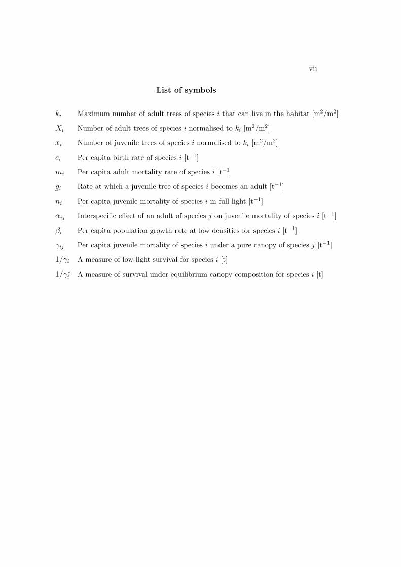
List of symbols
ki Maximum number of adult trees of species i that can live in the habitat [m2/m2]
Xi Number of adult trees of species i normalised to ki [m2/m2]
xi Number of juvenile trees of species i normalised to ki [m2/m2]
ci Per capita birth rate of species i [t−1]
mi Per capita adult mortality rate of species i [t−1]
gi Rate at which a juvenile tree of species i becomes an adult [t−1]
ni Per capita juvenile mortality of species i in full light [t−1]
αij Interspecific effect of an adult of species j on juvenile mortality of species i [t−1]
βi Per capita population growth rate at low densities for species i [t−1]
γij Per capita juvenile mortality of species i under a pure canopy of species j [t−1]
1/γi A measure of low-light survival for species i [t]
1/γ∗i A measure of survival under equilibrium canopy composition for species i [t]

viii
Contents
1 Introduction 1
1.1 An overview on vegetation models . . . . . . . . . . . . . . . . 1
1.2 Models on forest dynamics . . . . . . . . . . . . . . . . . . . . 6
1.3 Coexistence . . . . . . . . . . . . . . . . . . . . . . . . . . . . 9
1.4 Shade tolerance and successional status . . . . . . . . . . . . . 11
1.5 Aim of the thesis . . . . . . . . . . . . . . . . . . . . . . . . . 15
2 The model 17
2.1 Model derivation . . . . . . . . . . . . . . . . . . . . . . . . . 17
2.2 Model predictions - one species . . . . . . . . . . . . . . . . . 24
2.3 Model predictions - two species . . . . . . . . . . . . . . . . . 27
2.3.1 Coexistence: the role of shade tolerance . . . . . . . . . 30
2.3.2 Coexistence: relative abundances . . . . . . . . . . . . 36
2.3.3 Founder control . . . . . . . . . . . . . . . . . . . . . . 40
2.4 Model predictions - three species . . . . . . . . . . . . . . . . 43
3 Comparisons with other models 49
3.1 Classical competition . . . . . . . . . . . . . . . . . . . . . . . 49
3.2 Implicit space structure . . . . . . . . . . . . . . . . . . . . . . 50
3.3 Lottery models . . . . . . . . . . . . . . . . . . . . . . . . . . 53
ix
x CONTENTS
3.4 Resource competition . . . . . . . . . . . . . . . . . . . . . . . 54
3.5 Size structure . . . . . . . . . . . . . . . . . . . . . . . . . . . 55
4 Model applications 63
4.1 Introduction . . . . . . . . . . . . . . . . . . . . . . . . . . . . 63
4.2 Beech-maple communities . . . . . . . . . . . . . . . . . . . . 64
4.3 Patchiness . . . . . . . . . . . . . . . . . . . . . . . . . . . . . 69
4.4 Forest succession . . . . . . . . . . . . . . . . . . . . . . . . . 72
5 Concluding remarks 79
5.1 Model structure . . . . . . . . . . . . . . . . . . . . . . . . . . 79
5.2 Model results . . . . . . . . . . . . . . . . . . . . . . . . . . . 83
Bibliography 88

Chapter 1
Introduction
The present thesis deals with mathematical models of forest dynamics. This
chapter is devoted to a short introduction on concepts and ideas about forest
modelling for temperate forests.
1.1 An overview on vegetation models
A vegetation model is a conceptual scheme based on stated relationships
between the “actors” (e.g., plant species, nutrients, physical quantities) of
the system that has to be modelled. Generally, the goal of a model is either
to understand observed patterns or to predict system’s behaviours.
The outcomes of vegetation models range from the leaf scale (e.g., photo-
synthesis, gas exchange) to the planetary scale (e.g., plant distribution along
climatic gradients, feedback with climate).
In all cases, the building of a model, follows the general Occam’s razor
principle.1 In few words, this principle states that the simplest explanation
1The principle is attributed to 14th-century English logician, theologian and Franciscan
friar, William of Ockham.
1
2 CHAPTER 1. INTRODUCTION
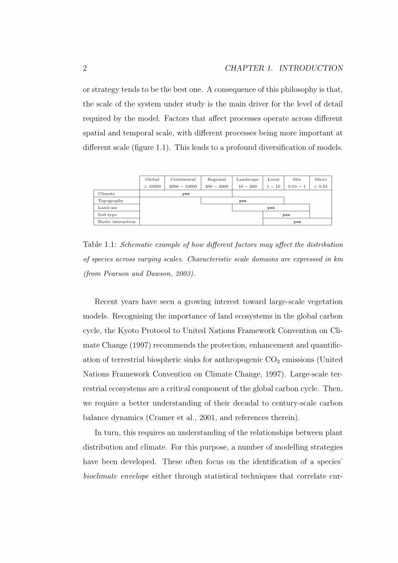
or strategy tends to be the best one. A consequence of this philosophy is that,
the scale of the system under study is the main driver for the level of detail
required by the model. Factors that affect processes operate across different
spatial and temporal scale, with different processes being more important at
different scale (figure 1.1). This leads to a profound diversification of models.
Global Continental Regional Landscape Local Site Micro
> 10000 2000− 10000 200− 2000 10− 200 1− 10 0.01− 1 < 0.01
Climate yes
Topography yes
Land-use yes
Soil type yes
Biotic interaction yes
Table 1.1: Schematic example of how different factors may affect the distribution
of species across varying scales. Characteristic scale domains are expressed in km
(from Pearson and Dawson, 2003).
Recent years have seen a growing interest toward large-scale vegetation
models. Recognising the importance of land ecosystems in the global carbon
cycle, the Kyoto Protocol to United Nations Framework Convention on Cli-
mate Change (1997) recommends the protection, enhancement and quantific-
ation of terrestrial biospheric sinks for anthropogenic CO2 emissions (United
Nations Framework Convention on Climate Change, 1997). Large-scale ter-
restrial ecosystems are a critical component of the global carbon cycle. Then,
we require a better understanding of their decadal to century-scale carbon
balance dynamics (Cramer et al., 2001, and references therein).
In turn, this requires an understanding of the relationships between plant
distribution and climate. For this purpose, a number of modelling strategies
have been developed. These often focus on the identification of a species’
bioclimate envelope either through statistical techniques that correlate cur-

1.1. AN OVERVIEW ON VEGETATION MODELS 3
rent species distribution with climate variables (e.g., Pearson and Dawson,
2003; Thuiller, 2003) or through an understanding of species physiological
responses to climate (e.g., Woodward, 1987). Having identified a species’
climate envelope, the applications of scenarios of future climate enables the
potential redistribution of species’ climate space to be estimated (Pearson
and Dawson, 2003).
Recent studies have questioned the validity of the bioclimate envelope
approach by pointing to the many factors other than climate – mainly biotic
interactions such as competition – that play an important part in determining
species distributions and their dynamics over time (Davis et al., 1998).
Such factors are often dealt with by another class of computer models.
In the case of forests, this models are known as gap (or patch) models (see a
review in Bugmann, 2001). But because these models are individual-based,
they cannot describe the large-scale dynamics. This would require simulating
every tree on the region under study, which would be immensely computa-
tionally demanding.
A current challenge is to understand how climate change, as well as nat-
ural disturbances, affect vegetation dynamics and ecosystem processes. One
of the high priority activities of the International Geosphere-Biosphere Pro-
gramme (IGBP) – the core project of the Global Change and Terrestrial
Ecosystems (GCTE) – is to develop a new class of dynamic biogeography
models, known as DGVMs2 (Steffen et al., 1992, 1996). The primary frame-
work for a DGVM was outlined by Prentice and GVDM Members (1989)
over two decades ago. Based on a linkage between an equilibrium global ve-
getation model and smaller scale ecosystem dynamics modules, Steffen et al.
(1996) proposed the structure of a first generation DGVM that simulates
2Dynamic Global Vegetation Models
4 CHAPTER 1. INTRODUCTION
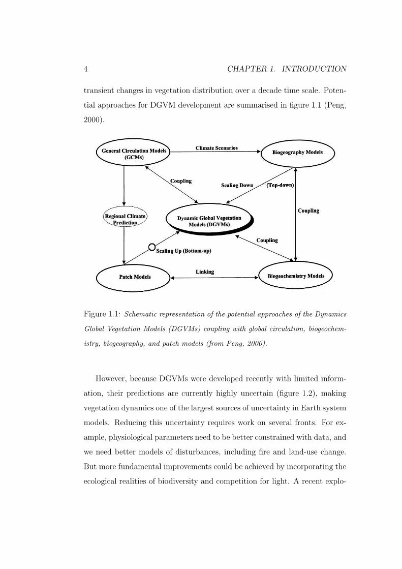
transient changes in vegetation distribution over a decade time scale. Poten-
tial approaches for DGVM development are summarised in figure 1.1 (Peng,
2000).
Figure 1.1: Schematic representation of the potential approaches of the Dynamics
Global Vegetation Models (DGVMs) coupling with global circulation, biogeochem-
istry, biogeography, and patch models (from Peng, 2000).
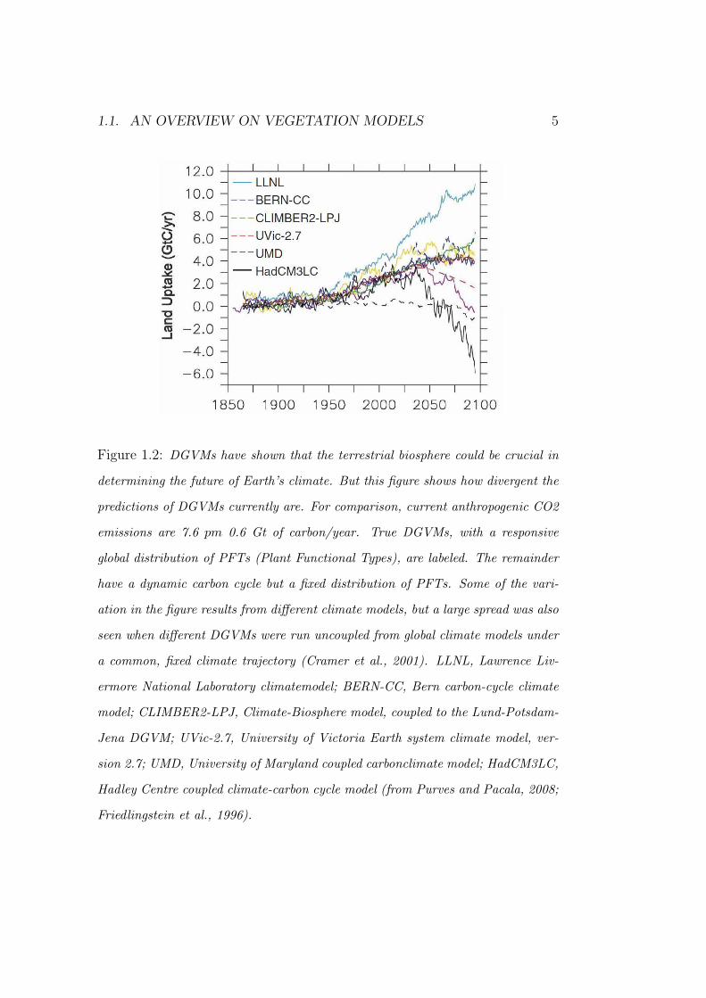
However, because DGVMs were developed recently with limited inform-
ation, their predictions are currently highly uncertain (figure 1.2), making
vegetation dynamics one of the largest sources of uncertainty in Earth system
models. Reducing this uncertainty requires work on several fronts. For ex-
ample, physiological parameters need to be better constrained with data, and
we need better models of disturbances, including fire and land-use change.
But more fundamental improvements could be achieved by incorporating the
ecological realities of biodiversity and competition for light. A recent explo-
1.1. AN OVERVIEW ON VEGETATION MODELS 5
Figure 1.2: DGVMs have shown that the terrestrial biosphere could be crucial in
determining the future of Earth’s climate. But this figure shows how divergent the
predictions of DGVMs currently are. For comparison, current anthropogenic CO2
emissions are 7.6 pm 0.6 Gt of carbon/year. True DGVMs, with a responsive
global distribution of PFTs (Plant Functional Types), are labeled. The remainder
have a dynamic carbon cycle but a fixed distribution of PFTs. Some of the vari-
ation in the figure results from different climate models, but a large spread was also
seen when different DGVMs were run uncoupled from global climate models under
a common, fixed climate trajectory (Cramer et al., 2001). LLNL, Lawrence Liv-
ermore National Laboratory climatemodel; BERN-CC, Bern carbon-cycle climate
model; CLIMBER2-LPJ, Climate-Biosphere model, coupled to the Lund-Potsdam-
Jena DGVM; UVic-2.7, University of Victoria Earth system climate model, ver-
sion 2.7; UMD, University of Maryland coupled carbonclimate model; HadCM3LC,
Hadley Centre coupled climate-carbon cycle model (from Purves and Pacala, 2008;
Friedlingstein et al., 1996).
6 CHAPTER 1. INTRODUCTION
sion in forest inventory data might make this possible (Purves and Pacala,
2008).
DGVMs could be substantially improved by basing them on the height-
structured individual-based models (IBMs) (e.g., Pacala et al., 1993). How-
ever, as I said before, IBMs are too complex to run at large scale. A more
efficient approach would be to derive suitable mathematical equations to
scale correctly from parameters governing individual trees to the dynamics
of forested region (Kohyama et al., 2001; Hurtt et al., 1998; Moorcroft et al.,
2001; Kohyama, 2005). This step in DGVMs development is depicted by the
arrow marked with a circle in figure 1.1.
1.2 Models on forest dynamics
An understanding of interactions at the population level (e.g., competition) is
of importance not only as a part of global vegetation models. The description,
understanding and prediction of the long-term dynamics of forest ecosystems
has fascinated ecologists for a long time (e.g., Watt, 1947) and nowadays,
models of forest dynamics are perhaps the most widely studied class of models
in the ecological literature (Pacala et al., 1993). The vast majority of forest
models are derived from the computer model JABOWA (Botkin et al., 1972).
They are termed gap or patch models.
The developers of JABOWA made a number of keys that allowed them to
formalise tree growth, tree establishment, and tree mortality in a relatively
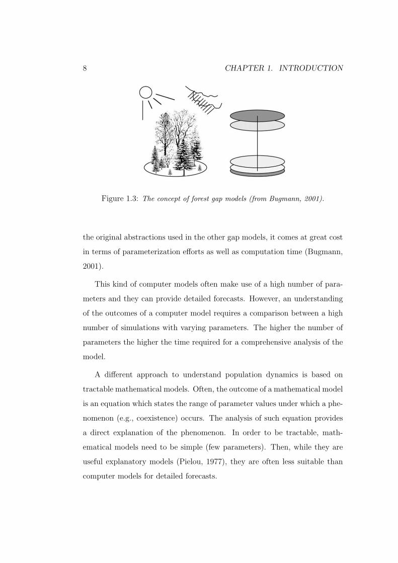
simple fashion (figure 1.3):
1. The forest stand is abstracted as a composite of many small patches
of land, where each can have a different age and successional stage.
The size of the patch is chosen so that a large individual organism can
1.2. MODELS ON FOREST DYNAMICS 7
dominate the entire patch; in the case of trees, patch size thus is on
the order of 100− 1000 m2.
2. Patches are horizontally homogeneous, i.e., tree position within a patch
is not considered. A consequence of this assumption is that all tree
crowns extend horizontally across the entire patch.
3. The leaves of each tree are located in an indefinitely thin layer (disk)
at the top of the stem.
4. Successional processes can be described on each of those patches sep-
arately, i.e., there are no interactions between patches, and the forest
is a mosaic of independent patches.
Additional basic features of JABOWA include the following: (5) the es-
tablishment, growth, and mortality of each individual tree is considered, i.e.,
the entity being modelled is the individual; (6) the model considers the tree
composition and size structure of the forest, but it does not deal with forest
functions such as biogeochemical cycling of carbon and nitrogen, or the flows
of water through the ecosystem; and (7) the competition between trees and
other life forms such as shrubs, herbs, or grasses is ignored (Bugmann, 2001).
A wide variety of formulations for growth processes, establishment, and
mortality factors have been developed in gap models over the past 30 years,
and modern gap models include more robust parameterizations of environ-
mental influences on tree growth and population dynamics as compared to
JABOWA. In particular, in the SORTIE model (Pacala et al., 1993), which
emphasises light competition as the major driver of forest succession, much
larger tracts of land are considered, and within this area the position of each
tree is kept track of to allow for the accurate calculation of light conditions.
Whereas the SORTIE approach certainly is more realistic and accurate than
8 CHAPTER 1. INTRODUCTION
Figure 1.3: The concept of forest gap models (from Bugmann, 2001).
the original abstractions used in the other gap models, it comes at great cost
in terms of parameterization efforts as well as computation time (Bugmann,
2001).
This kind of computer models often make use of a high number of para-
meters and they can provide detailed forecasts. However, an understanding
of the outcomes of a computer model requires a comparison between a high
number of simulations with varying parameters. The higher the number of
parameters the higher the time required for a comprehensive analysis of the
model.
A different approach to understand population dynamics is based on
tractable mathematical models. Often, the outcome of a mathematical model
is an equation which states the range of parameter values under which a phe-
nomenon (e.g., coexistence) occurs. The analysis of such equation provides
a direct explanation of the phenomenon. In order to be tractable, math-
ematical models need to be simple (few parameters). Then, while they are
useful explanatory models (Pielou, 1977), they are often less suitable than
computer models for detailed forecasts.

1.3. COEXISTENCE 9
Mathematical models on population dynamics are the core of this thesis
and they will be discussed extensively in the next chapters. They mostly
deal with coexistence.
1.3 Coexistence
How large numbers of competing plant species manage to coexist is a major
unresolved question in community ecology (Silvertown, 2004). Doubts about
coexistence have been raised by the competitive exclusion principle. Roughly,
it states that if two species are too similar (e.g., they feed on the same re-
source), they cannot coexist (Hardin, 1960). This principle is based on theory
(see the third chapter) and has been tested only in laboratory experiments
(e.g., Tilman and Wedin, 1991, for the case of grasses). However, ecologists
are confronted with many examples of different species living together and
apparently sharing the same resources. Thus, they included in their model
a lot of different ideas and hypotheses to explain coexistence (reviewed in
DeAngelis and Waterhouse, 1987; Chesson, 2000; Silvertown, 2004).
Hypothesised mechanisms include (among others): functional interac-
tions between species (Vance, 1984), trade-off between strategies (Shmida
and Ellner, 1984; Tilman, 1994), the effect of spatial extent (Yodzis, 1978),
disturbance patterns (Huston, 1979), the effect of integrating small-scale sys-
tems into large landscapes (Levins, 1969; Taneyhill, 2000), differential re-
sponses to spatial and temporal variability of the environment (Pacala and
Tilman, 1994), the effect of an open habitat with immigration (Shmida and
Ellner, 1984) and facilitation (Bruno et al., 2003). According to the high
complexity of this topic, it does not exist a general theory of coexistence,
rather there are different approaches depending on the characteristics of the
10 CHAPTER 1. INTRODUCTION
system under study (e.g. scale, the type of resources, etc...).
In particular, in the case of forest models, the effect of fluctuations in
environmental conditions have been considered by Kelly and Bowler (2002)
and much attention has been devoted to the role of size structure in the
competition for light (Kohyama, 1992, 1993; Strigul et al., 2008; Adams et al.,
2007). These size-structured models show that coexistence is possible even in
the case of many tree species competing for light. But, generally, they cannot
be completely solved and this complicates the analysis of mechanisms behind
coexistence.
Despite the efforts outlined above, there is still debate on mechanisms
behind coexistence, specially in the co-dominance of highly shade tolerant
trees (e.g., Gravel et al., 2008). In many forest communities of North Amer-
ica external disturbances such as windstorms and fires, probably account for
a small minority of tree-for-tree replacements over any long period of time.
Moreover, gradients in the physical environment often can be neglected (Fox,
1977). In these cases neither external disturbances nor environmental het-
erogeneity should be used to explain coexistence.
A well-known example is the case of beech-maple communities (Forcier,
1975; Fox, 1977; Woods, 1979; Chyper and Boucher, 1982; Canham, 1989,
1990; Poulson and Platt, 1996; Gravel et al., 2008). From the studies that I
have considered, three different hypotheses to explain coexistence emerge.
The studies of Fox (1977), Woods (1979) and Chyper and Boucher (1982)
support the idea of coexistence based on reciprocal replacement. In contrast,
other studies (Forcier, 1975; Canham, 1989, 1990; Poulson and Platt, 1996)
support the idea of coexistence based both on a trade-off between strategies
and on external fluctuations. Finally, the study of Gravel et al. (2008) points
out that the high level of similarity between species in terms of their response

1.4. SHADE TOLERANCE AND SUCCESSIONAL STATUS 11
under the relatively limited range of conditions that are typically encountered
in a single stand, precludes a deterministic interpretation of coexistence, at
least at a local scale (Gravel et al., 2008).
1.4 Shade tolerance and successional status
Forest dynamics cannot be understood without a clear vision of three closely
related concepts: shade tolerance, gap dynamics and successional status.
They are general concepts used in a wide range of circumstances, in this
section I discuss how these concepts are considered in this thesis.
Shade tolerance is an ecological concept that refers to the capacity of
a given plant to tolerate low light levels. It has been extensively studied
in forests, because light competition and interspecific differences in shade
tolerance are often important determinants of forest structure and dynamics
(Horn, 1971; Canham et al., 1994; Gravel et al., 2008).
Gap dynamics can be described as follows: a forest is a mosaic of tree
crowns. The individual trees that are the elements of this mosaic dominate
the resources and block the growth of young trees. When they die and open
a gap in the canopy, a number of responses are initiated in the small area
below the canopy opening. These responses eventually lead to the repair of
the forest canopy. The tolerance of juvenile tree species is of importance, not
in allowing net growth beneath the canopy, but in allowing them to survive
through long periods of suppression (e.g., Canham, 1989).
Thus, gap dynamics describes how competition works while the shade
tolerance is a key feature describing the competitive ability of tree species.
The result of competition determines the successional status of a tree species.
However, from a quantitative point of view, shade tolerance lacks a univocally

12 CHAPTER 1. INTRODUCTION
accepted definition (Valladares and Niinemets, 2008). In particular, there is
not a clear difference between shade tolerance and successional status. For
example, Horn (1971) wrote:
“Foresters long ago stated the first axiom of the effects of shading
on forest succession: species that are progressively more shade
tolerant become dominant as succession proceeds towards climax.
Unfortunately, the measurement of tolerance that foresters often
use includes information about the stage of succession at which
the species in question is characteristically most abundant. Thus,
when the axiom is examined critically, it is found to be either
circular or unsupported, even though it is intuitively reasonable.”.
However, using a more objective measure of tolerance, Horn (1971) confirmed
that tolerance increases as succession proceeds.
A quantitative description of shade tolerance can be obtained in several
ways. From a physiological point of view, the shade tolerance of a given plant
is defined as the minimum light under which a plant can survive. A different
approach to define the shade tolerance is based on the well-known trade-off
between high-growth in high-light and high-growth in low-light shown in fig-
ure 1.4 (Bazzaz, 1979). Each of the two curves in figure 1.4 is defined by
two parameters: growth in low-light (the slope at zero light) and growth in
high-light (the maximum growth rate). These two parameters give a measure
of tolerance. Foresters have published extensive tables that place tree spe-
cies into categories of shade tolerance (Baker, 1949). Models derived from
JABOWA (see above) used these tables in their growth submodels. They
linked growth and shade tolerance on the basis of the relationship described
in figure 1.4.
However, Pacala et al. (1994) and Kobe et al. (1995) showed that the

1.4. SHADE TOLERANCE AND SUCCESSIONAL STATUS 13
Figure 1.4: Diameter growth rate versus light availability (from Pacala et al.,
1994).
linkage between shade tolerance and the growth abilities of figure 1.4 used in
the JABOWA models is at least questionable (Pacala et al., 1993). Indeed,
they estimated growth and mortality functions for nine species. Then, they
plotted the nine species in a two-dimensional parameter space according to
both low-light growth versus high-light growth (figure 1.5a) and high-light
growth versus low-light survival (figure 1.5b). What is especially significant
about the axis in figure 1.5b is that the species order according to their
successional status. On the other hand, it is important to note that species do
not order according to successional status when viewed in terms of low- and
high- light growth abilities (figure 1.5a). Kobe et al. (1995) suggested that
low-light survival rather than low-light growth should be used as a component
of shade tolerance. Note that in doing so, they equated the concepts of shade
tolerance and successional status.

14 CHAPTER 1. INTRODUCTION
(a) (b)
Figure 1.5: Scatter plot of nine species according to their estimated attributes
(from Kobe et al., 1995).
In this view shade tolerance is related to species-specific parameters. In
contrast, Valladares and Niinemets (2008) argued that shade tolerance is not
an absolute value of, say, the minimum light availability required by a given
species, but a relative concept that depends on the specific ecological context.
Moreover, Horn (1971) pointed out that there is no reason to believe that
the tolerance orders at a particular stage of succession (i.e., under a given
canopy composition) are the same at any other stage or under other environ-
mental conditions. In this thesis the shade tolerance is a relative concept as
well: I consider the shade tolerance equivalent to survival in low-light, where
survival in low-light is a function of understory light availability rather than
a species-specific parameter. Then, through light transmissivity of canopy
trees, the shade tolerance of a given tree species depends on canopy com-
position. This is of importance if different tree species have different light
transmissivity through canopy. Indeed, Canham et al. (1994) found signific-
ative interspecific variation in light transmission by canopy trees. Moreover,
1.5. AIM OF THE THESIS 15
Pacala et al. (1994) and Kobe et al. (1995) pointed out that this interspe-
cific variation in light transmissivity has the potential to significatively affect
growth rate and mortality of understory saplings even in the case of shade
tolerant trees, thus playing a key role on the overall dynamics.
1.5 Aim of the thesis
The aim of this thesis is to develop and analyse a simple mathematical model
that is able to account for mechanisms and behaviours discussed in the last
two sections. In particular, as I am interested in explaining coexistence mech-
anisms as a result of the internal structure of the forest community, I focus
on a homogeneous closed environment. That is, I neglect mechanisms such
as: stochastic disturbances, environmental heterogeneity and immigration.
These mechanisms have been studied elsewhere (e.g., Huston, 1979; Kelly
and Bowler, 2002; Shmida and Ellner, 1984). This thesis deals mainly with
coexistence of shade tolerant tree species, the role of interspecific variation
in light transmissivity by canopy trees on the overall dynamics and the rela-
tionship between shade tolerance and successional status. These topics are of
importance both from a theoretical point of view and in determining which
are the important interactions that have to be considered in more complex
predictive models. For example, a major result of this thesis states that, in
order to describe coexistence, a critical feature is the interspecific variation
in light transmissivity rather than the trade-off between abilities in low- and
high-light.

16 CHAPTER 1. INTRODUCTION
Chapter 2
The model
In this chapter I will derive a simple mechanistic model to describe forest
dynamics. The model is based on competition for space. Two stage levels
are considered: adult and juvenile. Adult trees occupy space and cannot be
dislodged by juveniles. They cast shade on juveniles but they do not shade
each other. Juvenile trees have to survive in the adults shade and they grow
into the canopy only when a dominating adult dies, thus releasing space.
2.1 Model derivation
In building the present model I followed the Levins’s approach: I ideally
divided a habitat into spatial cells; each cell can be either empty or occupied
by one adult individual. The dynamics of occupancy of the habitat is then
described by the following equation (Levins, 1969):
dx
dt= cx(1− x)−mx. (2.1)
Where x is the fraction of cells occupied by a species, c is the colonisation
rate and m is the mortality rate. A persistent population must satisfy the
17
18 CHAPTER 2. THE MODEL
condition c > m. Eventually, it will approach the equilibrium density given
by x = 1−m/c.
In the original interpretation (Levins, 1969), cells were occupied by a
set of local populations called metapopulation (regional dynamic). However,
the extension to the local dynamic, where each cell has the size of an adult
individual, is straightforward (Klausmeir and Tilman, 2002).
I extended the Levins’s model by assuming that the tree population is
composed by two life history stages: adult and juvenile. Adults represent
dominant trees (canopy), while juveniles comprise seeds, seedlings and sap-
lings. It is important to note that this classification is hierarchical. Adults
and juveniles represent the two main levels of a forest: overstory and under-
story. When a juvenile tree reaches the canopy, it becomes an adult regard-
less of its age and size. I assumed that only adult trees can reproduce. This
assumption has been used also in other models (e.g., Adams et al., 2007).
Now, each cell has two levels: overstory and understory. On the overstory
level a cell can be either empty or occupied by one adult, while on the
understory level each cell can contain any number of juveniles of every species.
In order to keep mathematics simple, it is assumed that the space occupied
by a juvenile is negligible relative to the crown of an adult tree. I call empty
a cell with zero adults irrespective of the number of juveniles living there.
A juvenile can become an adult only in empty cells. Thus, it can either
colonise new areas (transient dynamics) or grow into recently vacated cells
(gap dynamics).
It is important to understand that in this scheme all adult trees are
exposed to full light (i.e., they have similar height), while juveniles are sup-
pressed if adult trees are present. That is, only juvenile mortality is affected
by crowding effect.
2.1. MODEL DERIVATION 19
The number of adults and juveniles is described by the state variables Pi
and pi, respectively; index i indicates the species. Then the following set of
equations describes the dynamics of n species (i = 1, . . . , n):
dPi
dt= g′i(S −
n∑j=1
sjPj)pi −miPi (2.2a)
dpi
dt= ciPi − g′i(S −
n∑j=1
sjPj)pi − (ni +n∑
j=1
α′ijPj)pi (2.2b)
Here, S is the total area of the habitat and sj is the mean1 area occupied
by an adult of species j (crown area). Then (S −∑
sjPj) is the portion of
space without adults where juveniles can grow into.
The number of adults increases by juvenile growth at the rate of g′i
(provided that empty cells are available) and decreases by mortality at the
rate mi. The number of juveniles increases by adult reproduction at the
rate ci and decreases either when juveniles grow into the adult class or by
mortality.
I assumed that the juvenile mortality rate depends linearly on adult dens-
ity. Then, ni represents the base mortality (when adults are absent), while
coefficients α′ij represent the effect of adults j on juveniles i. Generally, I
assumed that shading is the main effect of adults on juveniles. As a con-
sequence, α′ij is a compound measure of the shade projected by adults j and
the tolerance level of juveniles i (see section 2.3.1). Other kind of influences
will be discussed later in the text.
Let ki = S/si be the maximum number of adults i that can live in the
habitat. It is convenient to scale the number of both, adults and juveniles,
1Intuitively, in order for adult trees to fill the space, some plasticity in both crown shape
and crown size is required. Thus, two adult trees of the same species could have a different
crown area. However, I assumed that the mean crown area is a constant parameter (this
will be discussed in more detail in the discussion section).
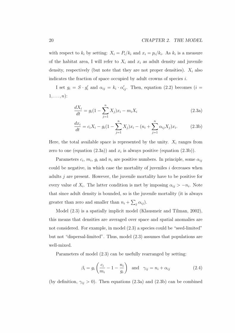
20 CHAPTER 2. THE MODEL
with respect to ki by setting: Xi = Pi/ki and xi = pi/ki. As ki is a measure
of the habitat area, I will refer to Xi and xi as adult density and juvenile
density, respectively (but note that they are not proper densities). Xi also
indicates the fraction of space occupied by adult crowns of species i.
I set gi = S · g′i and αij = ki · α′ij. Then, equation (2.2) becomes (i =
1, . . . , n):
dXi
dt= gi(1−
n∑j=1
Xj)xi −miXi (2.3a)
dxi
dt= ciXi − gi(1−
n∑j=1
Xj)xi − (ni +n∑
j=1
αijXj)xi. (2.3b)
Here, the total available space is represented by the unity. Xi ranges from
zero to one (equation (2.3a)) and xi is always positive (equation (2.3b)).
Parameters ci, mi, gi and ni are positive numbers. In principle, some αij
could be negative, in which case the mortality of juveniles i decreases when
adults j are present. However, the juvenile mortality have to be positive for
every value of Xi. The latter condition is met by imposing αij > −ni. Note
that since adult density is bounded, so is the juvenile mortality (it is always
greater than zero and smaller than ni +∑
j αij).
Model (2.3) is a spatially implicit model (Klausmeir and Tilman, 2002),
this means that densities are averaged over space and spatial anomalies are
not considered. For example, in model (2.3) a species could be “seed-limited”
but not “dispersal-limited”. Thus, model (2.3) assumes that populations are
well-mixed.
Parameters of model (2.3) can be usefully rearranged by setting:
βi = gi
(ci
mi
− 1− ni
gi
)and γij = ni + αij (2.4)
(by definition, γij > 0). Then equations (2.3a) and (2.3b) can be combined
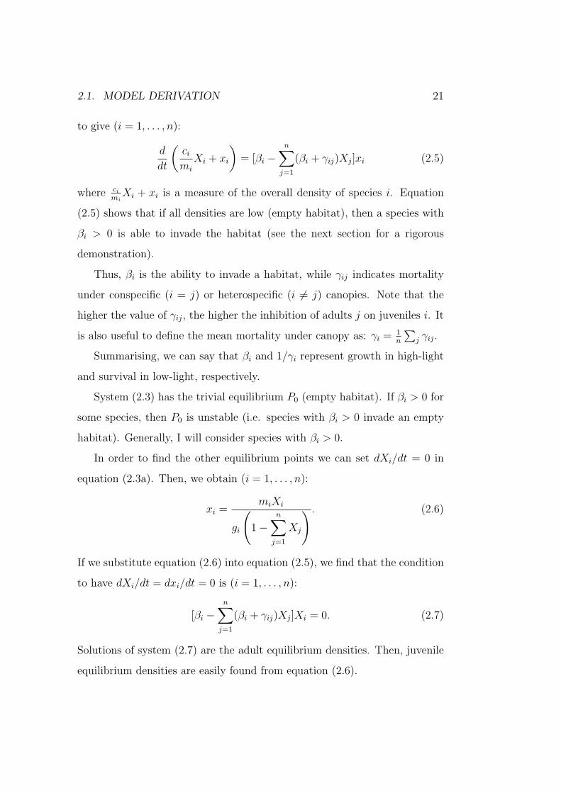
2.1. MODEL DERIVATION 21
to give (i = 1, . . . , n):
d
dt
(ci
mi
Xi + xi
)= [βi −
n∑j=1
(βi + γij)Xj]xi (2.5)
where ci
miXi + xi is a measure of the overall density of species i. Equation
(2.5) shows that if all densities are low (empty habitat), then a species with
βi > 0 is able to invade the habitat (see the next section for a rigorous
demonstration).
Thus, βi is the ability to invade a habitat, while γij indicates mortality
under conspecific (i = j) or heterospecific (i 6= j) canopies. Note that the
higher the value of γij, the higher the inhibition of adults j on juveniles i. It
is also useful to define the mean mortality under canopy as: γi = 1n
∑j γij.
Summarising, we can say that βi and 1/γi represent growth in high-light
and survival in low-light, respectively.
System (2.3) has the trivial equilibrium P0 (empty habitat). If βi > 0 for
some species, then P0 is unstable (i.e. species with βi > 0 invade an empty
habitat). Generally, I will consider species with βi > 0.
In order to find the other equilibrium points we can set dXi/dt = 0 in
equation (2.3a). Then, we obtain (i = 1, . . . , n):
xi =miXi
gi
(1−
n∑j=1
Xj
) . (2.6)
If we substitute equation (2.6) into equation (2.5), we find that the condition
to have dXi/dt = dxi/dt = 0 is (i = 1, . . . , n):
[βi −n∑
j=1
(βi + γij)Xj]Xi = 0. (2.7)
Solutions of system (2.7) are the adult equilibrium densities. Then, juvenile
equilibrium densities are easily found from equation (2.6).
22 CHAPTER 2. THE MODEL
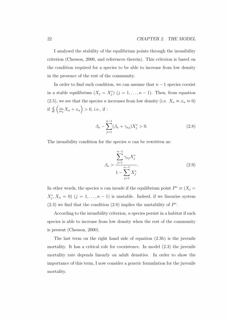
I analysed the stability of the equilibrium points through the invasibility
criterion (Chesson, 2000, and references therein). This criterion is based on
the condition required for a species to be able to increase from low density
in the presence of the rest of the community.
In order to find such condition, we can assume that n− 1 species coexist
in a stable equilibrium (Xj = X∗j ) (j = 1, . . . , n − 1). Then, from equation
(2.5), we see that the species n increases from low density (i.e. Xn ≈ xn ≈ 0)
if ddt
(cn
mnXn + xn
)> 0, i.e., if :
βn −n−1∑j=1
(βn + γnj)X∗j > 0. (2.8)
The invasibility condition for the species n can be rewritten as:
βn >
n−1∑j=1
γnjX∗j
1−n−1∑j=1
X∗j
. (2.9)
In other words, the species n can invade if the equilibrium point P ∗ ≡ (Xj =
X∗j , Xn = 0) (j = 1, . . . , n − 1) is unstable. Indeed, if we linearise system
(2.3) we find that the condition (2.8) implies the unstability of P ∗.
According to the invasibility criterion, n species persist in a habitat if each
species is able to increase from low density when the rest of the community
is present (Chesson, 2000).
The last term on the right hand side of equation (2.3b) is the juvenile
mortality. It has a critical role for coexistence. In model (2.3) the juvenile
mortality rate depends linearly on adult densities. In order to show the
importance of this term, I now consider a generic formulation for the juvenile
mortality.

2.1. MODEL DERIVATION 23
Let fi be the juvenile mortality rate for the species i. According to the
dependence of fi on adult density, I distinguished two cases (see Nakashizuka
and Kohyama, 1995):
fi = fi
(n∑
j=1
Xj
)additive model
fi = fi(X1, . . . , Xn) reciprocal model.
For example, if fi is a linear function, we will have fi = ni + αi(∑
j Xj) for
the additive model and fi = ni +∑
j αijXj for the reciprocal model (i.e. the
case of model (2.3)).
If juvenile mortality depends only on the total density of adults (i.e.
additive model), then coexistence is impossible. To show this fact I replaced
the juvenile mortality rate in system (2.3) by fi(∑
j Xj), then I set dXi/dt =
0, dxi/dt = 0 and xi 6= 0, Xi 6= 0. Rearranging terms, I obtained (i =
1, . . . , n):fi(∑
j Xj)
1−∑
j Xj
= gi
(ci
mi
− 1
). (2.10)
The system above can be rewritten simply as (i = 1, . . . , n):
n∑j=1
Xj = ωi (2.11)
where ωi is a combination of parameters of species i. In general, system
(2.11) has no non-trivial roots (except for some unlikely, meaningless sets
of parameters). Thus, an equilibrium with more than one species does not
exist, i.e. only one species can persist in the habitat. It is worth noting that
the additive model prevents coexistence for any functional form of juvenile
mortality.
In section 2.3.1 I will show that the additive model refers to the case
where no variation in interspecific transmissivity by canopy trees is allowed.
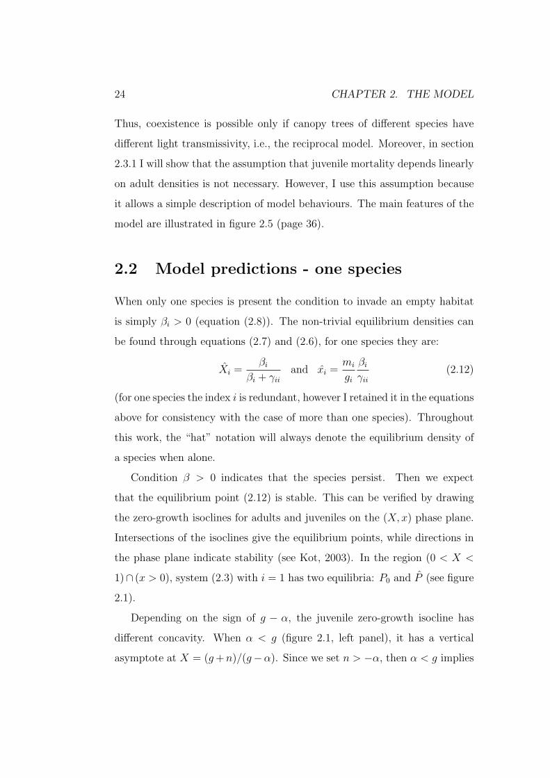
24 CHAPTER 2. THE MODEL
Thus, coexistence is possible only if canopy trees of different species have
different light transmissivity, i.e., the reciprocal model. Moreover, in section
2.3.1 I will show that the assumption that juvenile mortality depends linearly
on adult densities is not necessary. However, I use this assumption because
it allows a simple description of model behaviours. The main features of the
model are illustrated in figure 2.5 (page 36).
2.2 Model predictions - one species
When only one species is present the condition to invade an empty habitat
is simply βi > 0 (equation (2.8)). The non-trivial equilibrium densities can
be found through equations (2.7) and (2.6), for one species they are:
Xi =βi
βi + γii
and xi =mi
gi
βi
γii
(2.12)
(for one species the index i is redundant, however I retained it in the equations
above for consistency with the case of more than one species). Throughout
this work, the “hat” notation will always denote the equilibrium density of
a species when alone.
Condition β > 0 indicates that the species persist. Then we expect
that the equilibrium point (2.12) is stable. This can be verified by drawing
the zero-growth isoclines for adults and juveniles on the (X, x) phase plane.
Intersections of the isoclines give the equilibrium points, while directions in
the phase plane indicate stability (see Kot, 2003). In the region (0 < X <
1)∩ (x > 0), system (2.3) with i = 1 has two equilibria: P0 and P (see figure
2.1).
Depending on the sign of g − α, the juvenile zero-growth isocline has
different concavity. When α < g (figure 2.1, left panel), it has a vertical
asymptote at X = (g +n)/(g−α). Since we set n > −α, then α < g implies
2.2. MODEL PREDICTIONS - ONE SPECIES 25
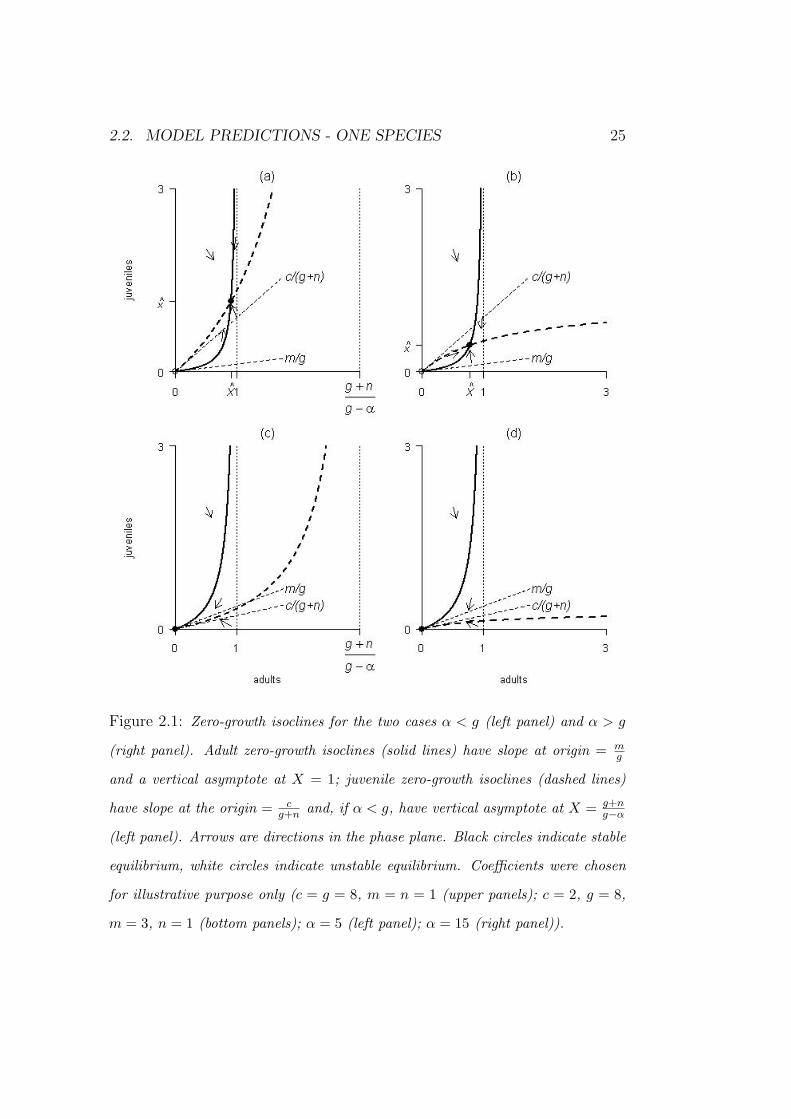
Figure 2.1: Zero-growth isoclines for the two cases α < g (left panel) and α > g
(right panel). Adult zero-growth isoclines (solid lines) have slope at origin = mg
and a vertical asymptote at X = 1; juvenile zero-growth isoclines (dashed lines)
have slope at the origin = cg+n and, if α < g, have vertical asymptote at X = g+n
g−α
(left panel). Arrows are directions in the phase plane. Black circles indicate stable
equilibrium, white circles indicate unstable equilibrium. Coefficients were chosen
for illustrative purpose only (c = g = 8, m = n = 1 (upper panels); c = 2, g = 8,
m = 3, n = 1 (bottom panels); α = 5 (left panel); α = 15 (right panel)).

26 CHAPTER 2. THE MODEL
Figure 2.2: Schematic representation of adult (solid line) and juvenile (dashed
line) zero growth isoclines. See the text for the meaning of thick arrows.
that (g + n)/(g − α) > 1. As a consequence, through an inspection of figure
2.1, it is clear that when c/(g + n) > m/g (i.e. β > 0) the species persists,
and approaches the stable equilibrium P . On the other hand, if β < 0 then
P disappears and P0 becomes stable.
It is worth noting that α does not affect the persistence condition, while it
determines the equilibrium density. Low values of α correspond to high levels
of tolerance relative to the shade of conspecific adults. Figure 2.1 (upper
panels) shows two juveniles zero-growth isoclines with different values of α;
it is clear that the higher the tolerance, the higher the equilibrium density
or, equivalently, the denser is the canopy (see also equations (2.12)). Such a
relationship is widely observed (Horn, 1971).
2.3. MODEL PREDICTIONS - TWO SPECIES 27
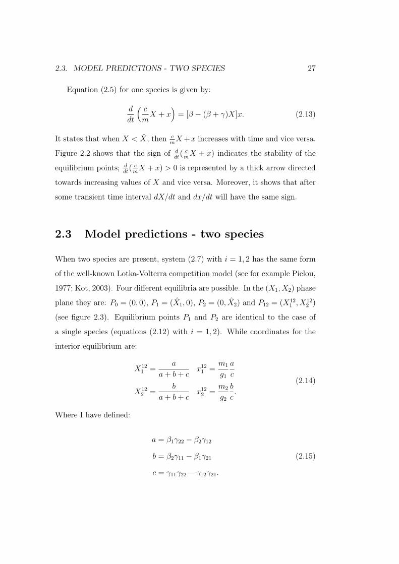
Equation (2.5) for one species is given by:
d
dt
( c
mX + x
)= [β − (β + γ)X]x. (2.13)
It states that when X < X, then cm
X +x increases with time and vice versa.
Figure 2.2 shows that the sign of ddt
( cm
X + x) indicates the stability of the
equilibrium points; ddt
( cm
X + x) > 0 is represented by a thick arrow directed
towards increasing values of X and vice versa. Moreover, it shows that after
some transient time interval dX/dt and dx/dt will have the same sign.
2.3 Model predictions - two species
When two species are present, system (2.7) with i = 1, 2 has the same form
of the well-known Lotka-Volterra competition model (see for example Pielou,
1977; Kot, 2003). Four different equilibria are possible. In the (X1, X2) phase
plane they are: P0 = (0, 0), P1 = (X1, 0), P2 = (0, X2) and P12 = (X121 , X12
2 )
(see figure 2.3). Equilibrium points P1 and P2 are identical to the case of
a single species (equations (2.12) with i = 1, 2). While coordinates for the
interior equilibrium are:
X121 =
a
a + b + cx12
1 =m1
g1
a
c
X122 =
b
a + b + cx12
2 =m2
g2
b
c.
(2.14)
Where I have defined:
a = β1γ22 − β2γ12
b = β2γ11 − β1γ21 (2.15)
c = γ11γ22 − γ12γ21.
28 CHAPTER 2. THE MODEL
Here, I consider the case with both β1 > 0 and β2 > 0. Then, for what I said
in the previous section it is clear that P0 is unstable i.e., at least one species
occupies the habitat.
Equations (2.9) states that Pi is unstable if (i = 1, 2, j 6= i):
βj > γjiXi
1− Xi
. (2.16)
It is important to stress that the condition above means that a species j
is able to invade a monoculture of species i. Using equation (2.12) it can be
conveniently rewritten as:
βj
γji
>βi
γii
(2.17)
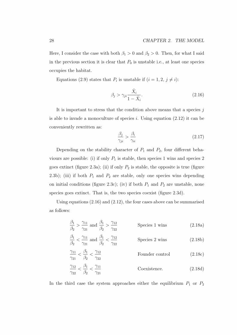
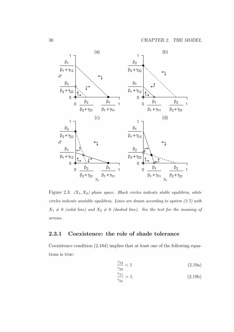
Depending on the stability character of P1 and P2, four different beha-
viours are possible: (i) if only P1 is stable, then species 1 wins and species 2
goes extinct (figure 2.3a); (ii) if only P2 is stable, the opposite is true (figure
2.3b); (iii) if both P1 and P2 are stable, only one species wins depending
on initial conditions (figure 2.3c); (iv) if both P1 and P2 are unstable, none
species goes extinct. That is, the two species coexist (figure 2.3d).
Using equations (2.16) and (2.12), the four cases above can be summarised
as follows:
β1
β2
>γ11
γ21
andβ1
β2
>γ12
γ22
Species 1 wins (2.18a)
β1
β2
<γ11
γ21
andβ1
β2
<γ12
γ22
Species 2 wins (2.18b)
γ11
γ21
<β1
β2
<γ12
γ22
Founder control (2.18c)
γ12
γ22
<β1
β2
<γ11
γ21
Coexistence. (2.18d)
In the third case the system approaches either the equilibrium P1 or P2
2.3. MODEL PREDICTIONS - TWO SPECIES 29
depending on initial conditions, that is, the equilibrium is locally2 stable.
This behaviour is commonly termed founder control (Yodzis, 1978). In the
other three cases, the same equilibrium density is reached regardless of the
initial abundances of the two species, i.e., the three equilibria are globally
stable.
According to equations (2.5), the arrows in figure 2.3 represent the sign
of ddt
( ci
miXi + xi): if d
dt( ci
miXi + xi) > 0, then the arrow is directed towards
increasing Xi and vice versa. As dXi/dt and dxi/dt cannot have different sign
indefinitely (see figure 2.2), then such arrows indicate the stability character
of the equilibrium points. Thus, conditions (2.18c) and (2.18d) imply the
unstability and stability of P12, respectively. This result was confirmed by
numerical computation of eigenvalues for the jacobian matrix (not shown).
Condition (2.18d) implies that some degree of either intraspecific inhibi-
tion or interspecific facilitation is necessary in order to have coexistence. For
example, if αji < 0, then adults i increase the survival of juveniles j relative
to an empty habitat. We know that if βj < 0 species j cannot invade an
empty habitat, but we can ask if it can invade a habitat occupied by species
i when αji < 0. To answer this question we can consider the condition for
the unstability of Pi, i.e. equation (2.16). Right hand side of equation (2.16)
is always positive. Then, if βj < 0, species j can never invade a habitat, even
if it is facilitated by another species. Thus, the condition to invade an empty
habitat is always less restrictive than the condition to invade an occupied
one. Therefore, from a successional point of view, model (2.3) agrees with
the inhibition model of Connell and Slatyer (1977).
2An equilibrium point is locally stable if only a set of initial densities (i.e., a region in
the phase space) approaches it. Here, the term local refers to the phase space and not
to the real space. In contrast, if any initial density (i.e., any point in the phase space)
approaches the same equilibrium, the equilibrium point is said to be globally stable.
30 CHAPTER 2. THE MODEL
Figure 2.3: (X1, X2) phase space. Black circles indicate stable equilibria, white
circles indicate unstable equilibria. Lines are drawn according to system (2.7) with
X1 6= 0 (solid line) and X2 6= 0 (dashed line). See the text for the meaning of
arrows.
2.3.1 Coexistence: the role of shade tolerance
Coexistence condition (2.18d) implies that at least one of the following equa-
tions is true:
γ12
γ22
< 1 (2.19a)
γ11
γ21
> 1. (2.19b)
2.3. MODEL PREDICTIONS - TWO SPECIES 31
If γij < γjj, than adults j facilitate juveniles i relative to their offspring or,
equivalently, they inhibit their offspring relative to juveniles i. In few words,
coexistence is the result of interspecific facilitation or intraspecific inhibition,
where facilitation and inhibition are relative concepts.
There are two possibilities: I termed symmetric (relative) facilitation the
case when both equations (2.19) are true (species facilitate each other) and
asymmetric (relative) facilitation the case where only one of the equations
(2.19) is true (one species is facilitated, while the other is inhibited).
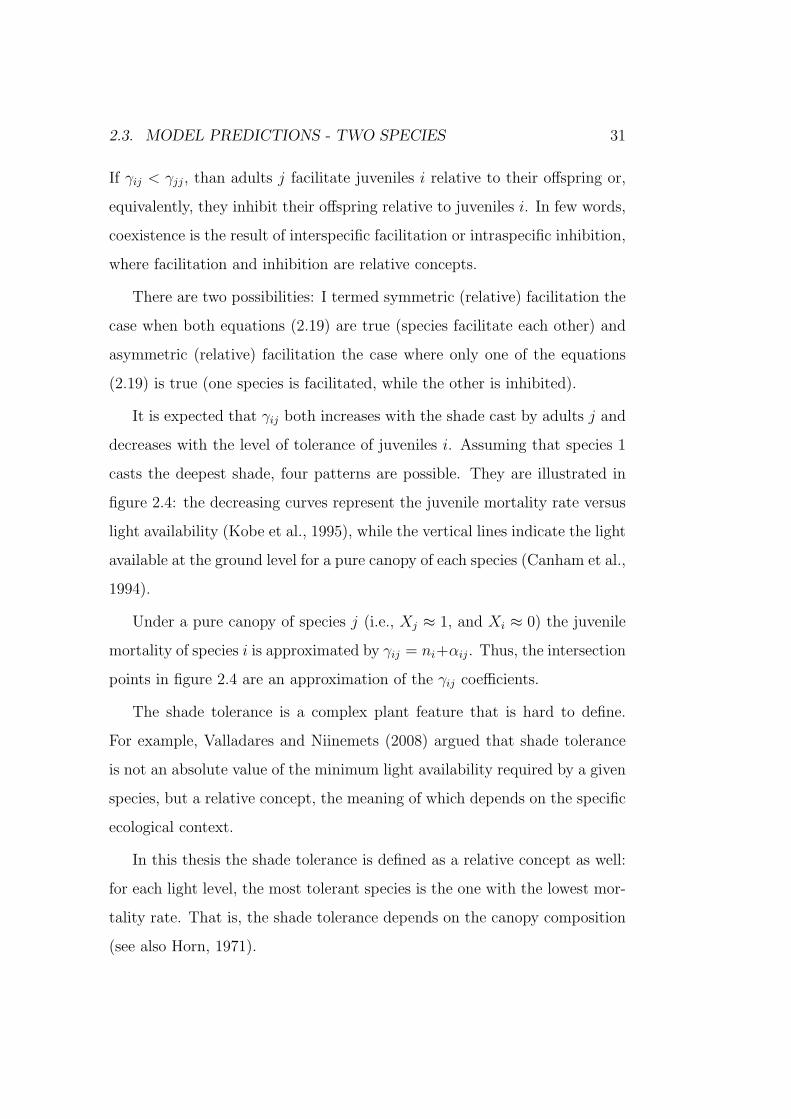
It is expected that γij both increases with the shade cast by adults j and
decreases with the level of tolerance of juveniles i. Assuming that species 1
casts the deepest shade, four patterns are possible. They are illustrated in
figure 2.4: the decreasing curves represent the juvenile mortality rate versus
light availability (Kobe et al., 1995), while the vertical lines indicate the light
available at the ground level for a pure canopy of each species (Canham et al.,
1994).
Under a pure canopy of species j (i.e., Xj ≈ 1, and Xi ≈ 0) the juvenile
mortality of species i is approximated by γij = ni+αij. Thus, the intersection
points in figure 2.4 are an approximation of the γij coefficients.
The shade tolerance is a complex plant feature that is hard to define.
For example, Valladares and Niinemets (2008) argued that shade tolerance
is not an absolute value of the minimum light availability required by a given
species, but a relative concept, the meaning of which depends on the specific
ecological context.
In this thesis the shade tolerance is defined as a relative concept as well:
for each light level, the most tolerant species is the one with the lowest mor-
tality rate. That is, the shade tolerance depends on the canopy composition
(see also Horn, 1971).
32 CHAPTER 2. THE MODEL
Figure 2.4b indicates symmetric facilitation. It depicts a situation in
which under a pure canopy of species 1, the juveniles of species 2 are more
tolerant than those of species 1, while the reverse is true under a pure canopy
of species 2. That is, the order of tolerance changes with the type of canopy.
In this case both the conditions (2.19) hold. Then, according to conditions
(2.18), either coexistence or competitive exclusion are possible. Note that in
this case coexistence is possible both with β1/β2 < 1 and β1/β2 > 1.
Figure 2.4: Schematic representation of juvenile mortality of both species 1 (solid
line) and species 2 (dashed line). Vertical lines represent the light available in
under a pure canopy of the two species. The x axis has a logarithmic scale.
2.3. MODEL PREDICTIONS - TWO SPECIES 33
In the case of figure 2.4a, none of the equations (2.19) is true, then glob-
ally stable coexistence is impossible. In this case there is not interspecific
facilitation. Depending on values of β1 and β2, either founder control or
competitive exclusion are possible (see conditions (2.18)).
Both figures 2.4c and 2.4d depict pattern of asymmetric facilitation. In
this case, depending on values of β1 and β2, all the conditions (2.18) could
be verified.
It is important to note that in the latter case coexistence requires a trade-
off between survival in understory and growth. For example, if species 1
casts the deepest shade and has generally higher tolerance (i.e., figure 2.4d),
then we have both γ12/γ22 < 1 and γ11/γ21 < 1. Then, condition (2.18d)
implies both 1/γ1 > 1/γ2 and β2 > β1. Thus, species 2 has lower survival in
low-light but higher growth in high-light.3 However, this trade-off promotes
coexistence only if the effects of adults on juvenile mortality are species
specific (i.e., the reciprocal model).
Note that, similarly to the Lotka-Volterra competition model, coexistence
within both symmetric and asymmetric facilitation requires that interspecific
facilitation is larger than intraspecific facilitation or, equivalently, that inter-
specific inhibition is lower than intraspecific inhibition (i.e., γ12γ21 < γ11γ22).
Finally, note that the dependence of juvenile mortality on light availability
and the crown transmissivity (i.e., the actors of figure 2.4) can be estimated
(see figures 4.2 at page 69 and 4.3 at page 70). Therefore, the γ coefficients
have a mechanistic interpretation and model (2.3) can be considered as a
simple mechanistic model for forest dynamics.
3In fact, in section 4.4, I will show that coexistence always requires a specific trade-off
between growth in high-light and survival in low-light, whether in the case of asymmetric
facilitation or symmetric facilitation.

34 CHAPTER 2. THE MODEL
The functional form of juvenile mortality in equation (2.3b) is based on
the following two linear approximations:
µi(L) = ai − biL (2.20)
and
L = 1− σ1X1 − σ2X2. (2.21)
Where µi(L) indicates the juvenile mortality of species i, L indicates light
availability in the understory (here L = 1 means full light), ai and bi are
parameters and 1/σi is a measure of canopy transmissivity by adult trees of
species i. Through the two equations above, the juvenile mortality can be
expressed as a function of adult densities fi(X1, X2):
fi(X1, X2) = ni + αi1X1 + αi2X2. (2.22)
Where ni = ai − bi, αi1 = biσ1 and αi2 = biσ2. From figure 4.3 at page 70 it
is seen that ni ' 0. Then, ai ' bi.
The higher the value of ai the lower is the general tolerance of species
i. Thus, a high value of bi indicates that the species i is generally intoler-
ant. Indeed, note that the coefficients αij are large if both the species i is
intollerant (i.e., high bi) and species j casts deep shade (i.e., high σj).
Compared with figure 4.3 (page 70), the approximation (2.20) is quite
rough. The functional forms described by equations (2.20) and (2.21) have
been chosen for the sake of simplicity. However, provided that (i=1,2):
µi(L) > 0dµi
dL< 0 (2.23a)
0 <L(X1, X2) < 1∂L
∂Xi
< 0, (2.23b)
any choice of L = L(X1, X2) and µi = µi(L) produces the same pattern
described by figure 2.3 (page 30). This, can be shown as follows:
2.3. MODEL PREDICTIONS - TWO SPECIES 35
I have set fi(X1, X2) = µi[L(X1, X2)]. Then, it follows that (i, j = 1, 2):
∂fi
∂Xj
=dµi
dL
∂L
∂Xi
> 0. (2.24)
The zero-growth isoclines depicted in figure 2.3 can be rewritten as:
Fi(X1, X2) = gi (2.25)
where I have set:
Fi(X1, X2) =fi(X1, X2)
1−X1 −X2
. (2.26)
Then, it is easy to show that:
∂Fi
∂Xi
> 0. (2.27)
Thus, the slope of the isoclines is given by:
dX2
dX1
= −
∂Fi
∂X1
∂Fi
∂X2
< 0. (2.28)
Moreover, the isoclines can be rewritten as:
fi(X1, X2) = gi(1−X1 −X2). (2.29)
As fi(X1, X2) > 0, the isoclines live in the region of the (X1, X2) phase plane
defined by X1 > 0, X2 > 0 and 1−X1 −X2 > 0.
The assumptions (2.23) are reasonable and very general but they fail to
exclude the possibility of multiple intersection of the isoclines. I shall hence-
forth cling to a third rather vague assumption that the functions Fi(X1, X2)
are sufficiently “well behaved” that multiple intersection do not occur (Vance,
1984). Figure 4.3 (page 70) suggests that this latter assumption is reasonable.
The main assumption of the model – the mean field approximation –
is that both space availability and understory light availability depend on
the mean densities of adult trees. Space availability affects juvenile growth
into the canopy while the understory light availability affects the survival of
juvenile trees. This is illustrated in figure 2.5.

36 CHAPTER 2. THE MODEL
Figure 2.5: Schematic view of the model
2.3.2 Coexistence: relative abundances
Within the coexistence conditions, species approach the equilibrium densities
given by equations (2.14). Using definitions (2.15), the ratio between adult
densities can be written as:
X∗1
X∗2
=β1γ22 − β2γ12
β2γ11 − β1γ21
, (2.30)
while the ratio between juvenile densities is:
x∗1x∗2
=m1g2
m2g1
X∗1
X∗2
(2.31)
(to simplify notation, I redefined X iji as X∗
i and xiji as x∗i ). Equation (2.31)
can be found directly by equations (2.6). It is simple but interesting: it
states that increasing values of m1g2/m2g1 both increase x∗1/x∗2 and decrease
X∗1/X
∗2 (see equations (2.4) and (2.30)).
2.3. MODEL PREDICTIONS - TWO SPECIES 37
Fox (1977) analysed five “climax” tree communities in North America,
each forest being dominated by two principal species. In most of cases he
found an inversion between overstory and understory abundances. Longer-
lived species were generally the more abundant in the overstory, but they
had a generally lower sapling abundance. Fox pointed out that this is not
obviously explained by seed year frequency, seed number or seed size (i.e.,
parameters ci in model (2.3)). Equation (2.31) suggests that this fact is
a consequence of the structure of the system. However, as X∗1/X
∗2 has a
complex dependence on all parameters, it is difficult to find the condition
which must be verified in order to have such an inversion. This obstacle can
be overcome by using the following approximation (i = 1, 2):
βi � 0 =⇒ βi ≈cigi
mi
=⇒ β1
β2
≈ c1g1m2
c2g2m1
. (2.32)
This means that both species are good invader of an empty habitat. Now,
I look for the conditions to have both X∗1/X
∗2 > 1 and x∗1/x
∗2 < 1. It is
convenient to think of X∗1/X
∗2 as a function of β1/β2, where the range of
β1/β2 is defined by equation (2.18d). Then equation (2.30) can be rewritten
as:
X∗1
X∗2
=γ22
γ21
β1
β2
− γ12
γ22
γ11
γ21
− β1
β2
. (2.33)
X∗1/X
∗2 is an increasing function of β1/β2. From equation (2.30) it is easy to
check that β1/β2 = γ1/γ2 implies X∗1/X
∗2 = 1. Moreover, condition (2.18d)
implies that γ12
γ22< γ1
γ2< γ11
γ21. Thus, figure 2.6 shows that:
γ1
γ2
<β1
β2
<γ11
γ21
=⇒ X∗1
X∗2
> 1. (2.34)
If x∗1/x∗2 < 1, then equation (2.31) can be rewritten as:
m2g1
m1g2
>X∗
1
X∗2
. (2.35)

38 CHAPTER 2. THE MODEL
Figure 2.6: Relative abundance X1/X2 as a function of β1/β2 in the range of
coexistence (solid line). The dashed line represents the straight line passing through
the origin which equation is y = (c2/c1) · (β1/β2).
Finally, through the approximation (2.32) and equation (2.33), equation
(2.35) becomes:
c2
c1
β1
β2
>γ22
γ21
β1
β2
− γ12
γ22
γ11
γ21
− β1
β2
=⇒ x∗1x∗2
< 1. (2.36)
Figure 2.6 shows that, provided c2/c1 > γ2/γ1, both conditions (2.34) and
(2.36) are verified if:
γ1
γ2
<β1
β2
< r, (2.37)
2.3. MODEL PREDICTIONS - TWO SPECIES 39
where I have defined:
r =
(c2
c1
γ11
γ21
− γ22
γ21
)+
√(c2
c1
γ11
γ21
− γ22
γ21
)2
+ 4c2
c1
γ12
γ21
2c2
c1
. (2.38)
Thus, provided that c2/c1 > γ2/γ1, the condition (2.37) implies both
X∗1/X
∗2 > 1 and x∗1/x
∗2 < 1.
It is important to note that in the case of symmetric facilitation (γ12/γ22 <
1 and γ11/γ21 > 1), it can be γ1/γ2 R 1. Thus, we can have the inversion of
abundances regardless of the relative magnitude of c1 and c2.
The inversion of abundances has a simple interpretation within the pat-
tern of reciprocal replacement: individuals leave the juvenile class either by
growth or death. Thus, juveniles that generally replace the shorter-lived
species, are expected to have lesser abundance in the understory.
At equilibrium the number of adults that die for each species per unit of
time, equals the number of juveniles of the same species that grows into the
canopy (see equation (2.3a)). If juveniles of one species always replace adults
of the other species (i.e., perfect reciprocal replacement), then the number
of adults of each species that die in the unit of time must be equal, i.e.:
m1X∗1 = m2X
∗2 . (2.39)
Within model (2.3), perfect reciprocal replacement is expected if γ12 � γ22,
γ11 � γ21, γ11 = γ22, c1 = c2 and g1 = g2. The latter two conditions imply
β1/β2 = m2/m1.4 Indeed, in this case, equation (2.33) can be approximated
by equation (2.39).
4approximation (2.32) has been used.

40 CHAPTER 2. THE MODEL
2.3.3 Founder control
In the case of founder control (condition (2.18c)), globally stable coexistence
of two species is impossible. Nonetheless, the species can still coexist in the
habitat through several locally stable equilibria.
Till now, I have considered the case of well-mixed populations living in
a habitat. However, “large-scale” spatial heterogeneity can be modelled by
considering a habitat of disjunct patches with only weak dispersal between
patches. In turn, a patch is taken to be a collection of contiguous cells capable
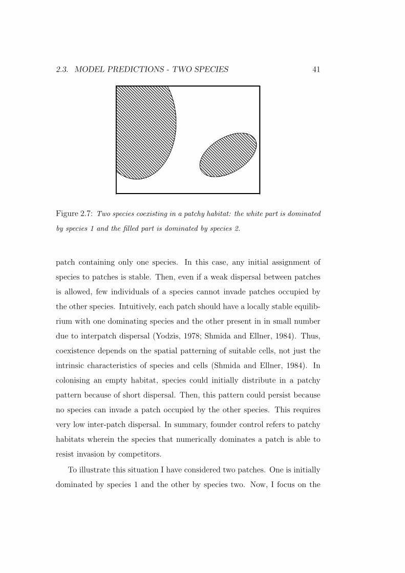
of supporting a single adult (see figure 2.7).
In the simplest scheme, all patches have the same size. Then, model (2.3)
can be applied to a generic patch rather than to the entire habitat.5
It is important to understand that, here, patchiness is a convenient way
to describe spatial heterogeneity due to internal factors, not to environmental
gradients. Thus, all model parameters have the same value in all patches of
the same size. That is, all patches are potentially identical.
Intuitively, if the dynamics of the generic patch is governed either by
two-species coexistence or competitive exclusion of one species by the other,
then all cells coalesce into a single, homogeneous habitat-patch which will
be dominated by the two species or by the stronger competitor, respectively.
But, if the dynamics of the generic patch is founder controlled (i.e., condition
(2.18c) holds), then the locally stable equilibria may be generated as follows.
Consider first a system of isolated patches (no interpatch dispersal), each
5Patches of different size have both different area and different carrying capacity (i.e.,
parameters S and ki in equation (2.2), respectively). Nevertheless, if approximation (2.32)
holds, then β1/β2 does not depend on S and if ni � αij and k1 = k2 (i.e., the species have
the same crown diameter), then γij/γjj does not depend on k. In such circumstances,
conditions (2.18) refer to all possible patches irrespective of size. Then, they refer to the
entire habitat as well.
2.3. MODEL PREDICTIONS - TWO SPECIES 41
Figure 2.7: Two species coexisting in a patchy habitat: the white part is dominated
by species 1 and the filled part is dominated by species 2.
patch containing only one species. In this case, any initial assignment of
species to patches is stable. Then, even if a weak dispersal between patches
is allowed, few individuals of a species cannot invade patches occupied by
the other species. Intuitively, each patch should have a locally stable equilib-
rium with one dominating species and the other present in in small number
due to interpatch dispersal (Yodzis, 1978; Shmida and Ellner, 1984). Thus,
coexistence depends on the spatial patterning of suitable cells, not just the
intrinsic characteristics of species and cells (Shmida and Ellner, 1984). In
colonising an empty habitat, species could initially distribute in a patchy
pattern because of short dispersal. Then, this pattern could persist because
no species can invade a patch occupied by the other species. This requires
very low inter-patch dispersal. In summary, founder control refers to patchy
habitats wherein the species that numerically dominates a patch is able to
resist invasion by competitors.
To illustrate this situation I have considered two patches. One is initially
dominated by species 1 and the other by species two. Now, I focus on the
42 CHAPTER 2. THE MODEL
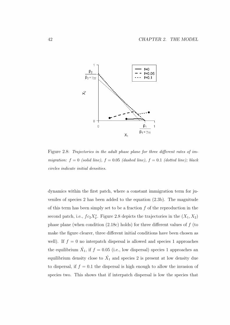
Figure 2.8: Trajectories in the adult phase plane for three different rates of im-
migration: f = 0 (solid line), f = 0.05 (dashed line), f = 0.1 (dotted line); black
circles indicate initial densities.
dynamics within the first patch, where a constant immigration term for ju-
veniles of species 2 has been added to the equation (2.3b). The magnitude
of this term has been simply set to be a fraction f of the reproduction in the
second patch, i.e., fc2X∗2 . Figure 2.8 depicts the trajectories in the (X1, X2)
phase plane (when condition (2.18c) holds) for three different values of f (to
make the figure clearer, three different initial conditions have been chosen as
well). If f = 0 no interpatch dispersal is allowed and species 1 approaches
the equilibrium X1, if f = 0.05 (i.e., low dispersal) species 1 approaches an
equilibrium density close to X1 and species 2 is present at low density due
to dispersal, if f = 0.1 the dispersal is high enough to allow the invasion of
species two. This shows that if interpatch dispersal is low the species that
2.4. MODEL PREDICTIONS - THREE SPECIES 43
numerically dominates a patch is able to resist invasion, thus allowing the
maintenance of a patchy habitat.
2.4 Model predictions - three species
A detailed analysis of dynamics with more than two species is beyond the
scope of this work. However, through simple considerations about equilib-
rium points for two species we can find the conditions for the coexistence of
three species.
When more than two species are considered several behaviours are pos-
sible. Here, I will consider only four simple examples. Results are similar to
those for more classical competition models (Huisman and Weissing, 2001).
Model (2.3) with n = 3 has eight possible equilibria: P0, Pi, Pij, Pijk
(i, j, k = 1, 2, 3; i 6= j 6= k). I consider βi > 0, i.e. P0 is unstable. Then, the
unstability of Pi and Pij means that none species goes extinct, i.e. all three
species coexist.
The tools that I have used to describe the coexistence of three species are
the following conditions:
βi
βj
> max
(γii
γji
,γij
γjj
)species i displaces species j (2.40a)
γij
γjj
<βi
βj
<γii
γji
species i and j coexist (2.40b)
I(k|i, j) > 0 species i and j are invaded by species k (2.40c)
where I defined I(k|i, j) ≡ βk− (βk +γki)Xiji − (βk +γkj)X
ijj . The conditions
above are the same as conditions (2.18a,b), (2.18d) and (2.8), respectively.
Note that condition (2.40c) makes sense if species i and j coexist when they
are alone.
44 CHAPTER 2. THE MODEL
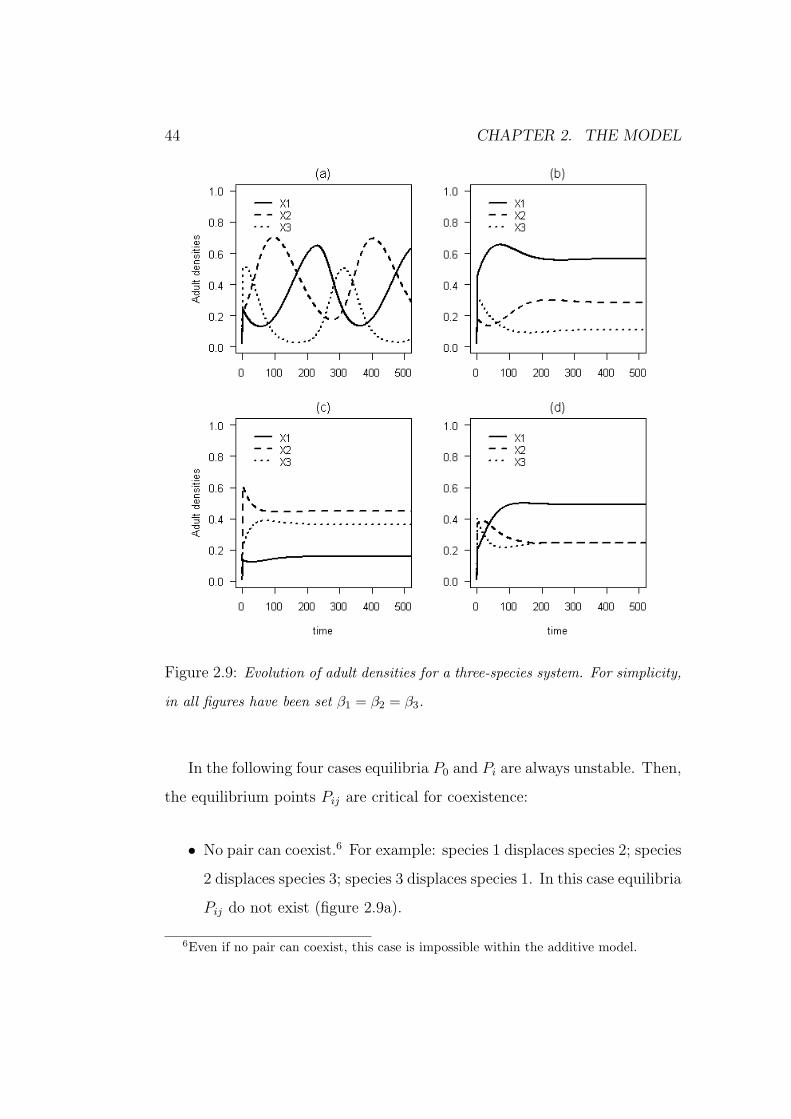
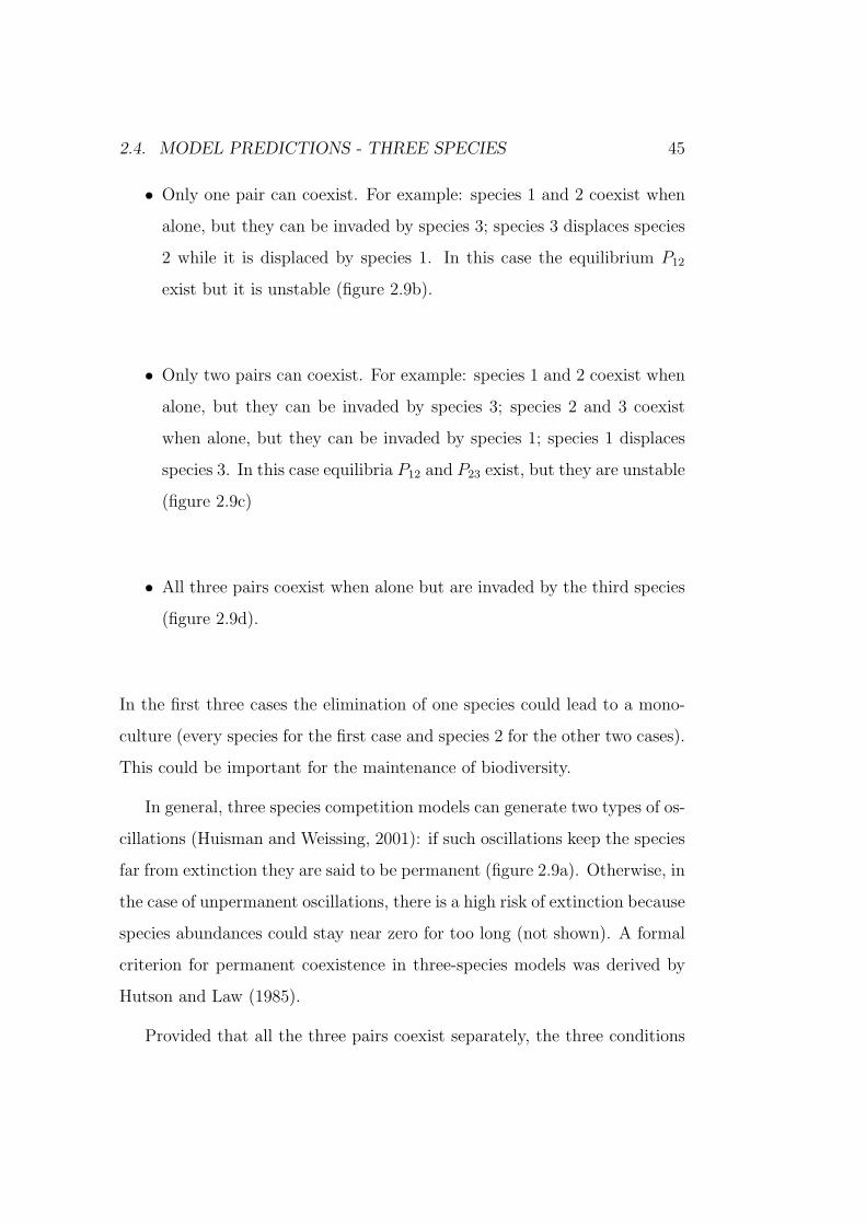
Figure 2.9: Evolution of adult densities for a three-species system. For simplicity,
in all figures have been set β1 = β2 = β3.
In the following four cases equilibria P0 and Pi are always unstable. Then,
the equilibrium points Pij are critical for coexistence:
• No pair can coexist.6 For example: species 1 displaces species 2; species
2 displaces species 3; species 3 displaces species 1. In this case equilibria
Pij do not exist (figure 2.9a).
6Even if no pair can coexist, this case is impossible within the additive model.
2.4. MODEL PREDICTIONS - THREE SPECIES 45
• Only one pair can coexist. For example: species 1 and 2 coexist when
alone, but they can be invaded by species 3; species 3 displaces species
2 while it is displaced by species 1. In this case the equilibrium P12
exist but it is unstable (figure 2.9b).
• Only two pairs can coexist. For example: species 1 and 2 coexist when
alone, but they can be invaded by species 3; species 2 and 3 coexist
when alone, but they can be invaded by species 1; species 1 displaces
species 3. In this case equilibria P12 and P23 exist, but they are unstable
(figure 2.9c)
• All three pairs coexist when alone but are invaded by the third species
(figure 2.9d).
In the first three cases the elimination of one species could lead to a mono-
culture (every species for the first case and species 2 for the other two cases).
This could be important for the maintenance of biodiversity.
In general, three species competition models can generate two types of os-
cillations (Huisman and Weissing, 2001): if such oscillations keep the species
far from extinction they are said to be permanent (figure 2.9a). Otherwise, in
the case of unpermanent oscillations, there is a high risk of extinction because
species abundances could stay near zero for too long (not shown). A formal
criterion for permanent coexistence in three-species models was derived by
Hutson and Law (1985).
Provided that all the three pairs coexist separately, the three conditions

46 CHAPTER 2. THE MODEL
(2.40c) can be written as:
(γ11γ22 − γ12γ21)β3 > β1(γ22γ31 − γ21γ32) + β2(γ11γ32 − γ12γ31) (2.41a)
(γ22γ33 − γ23γ32)β1 > β2(γ33γ12 − γ32γ13) + β3(γ22γ13 − γ23γ12) (2.41b)
(γ11γ33 − γ13γ31)β2 > β1(γ33γ21 − γ31γ23) + β3(γ11γ23 − γ13γ21). (2.41c)
System (2.41) looks quite ugly. However, it can be instructive to consider the
following special case. Assume that both species 1 and 2 are highly tolerant.
Moreover, assume that species 2 facilitates species 1, while species 1 inhibits
species 2 (i.e., the case of figure 2.4d). As we showed above, coexistence
implies a trade-off (i.e., β2 > β1). Now, assume that species 3 is highly
intolerant and that it has similar mortality under all three canopies (i.e.,
γ31 ≈ γ32 ≈ γ33, with γ33 > γ21). Finally, assume that species 3 casts a slight
shade which does not inhibit species 2 and 3 (i.e., γ13 ≈ γ23 ≈ 0). With the
last two assumptions the conditions (2.41) can be rewritten as:
β3 > γ33β1(γ22 − γ21) + β2(γ11 − γ12)
γ11γ22 − γ12γ21
(2.42a)
β1
β2
>γ12
γ22
(2.42b)
β1
β2
<γ11
γ21
. (2.42c)
Conditions (2.42b) and (2.42c) refer to the coexistence of species 1 and 2,
they are equivalent to condition (2.18d). Then, condition (2.42a) fixes a
threshold on β3 for the coexistence of all three species. Condition (2.42a)
can be rewritten as:
β3
β2
>γ33
γ21
(β1
β2
− γ12
γ22
)+
γ21
γ22
(γ11
γ21
− β1
β2
)γ11
γ21
− γ12
γ22
. (2.43)
As the two terms on right hand side are larger than one,7 the trade-off
between growth in high-light and survival in low-light is extended to the
7Figure 2.4d shows that γ21 > γ22.

2.4. MODEL PREDICTIONS - THREE SPECIES 47
three species system. That is, coexistence implies 1/γ1 > 1/γ2 > 1/γ3 and
β3 > β2 > β1.

48 CHAPTER 2. THE MODEL

Chapter 3
Comparisons with other models
An examination of differences and similarities with other approaches is a
useful way to understand the meaning of a model. In this chapter I compare
the model presented in this thesis with other mathematical models that try
to explain coexistence in a homogeneous environment.
3.1 Classical competition
The simplest competition model was developed by Lotka (1932) and Volterra
(1926). For two populations of size x1 and x2, it can be written as (i = 1, 2):
dxi
dt= ri(1− αi1x1 − αi2x2)xi. (3.1)
Coefficient ri represents the low-density growth for species i, αii represents
the inverse of the carrying capacity of species i when the other species is
absent and αij (i 6= j) describes the strength of the effect of species j on
species i. As mechanisms of interactions are not explicit, the system above
is phenomenological.
Provided that ri > 0, stable coexistence is possible only if α11 > α21 and
α22 > α12, that is, if interspecific effects are weak relative to intraspecific
49
50 CHAPTER 3. COMPARISONS WITH OTHER MODELS
effects (e.g., Kot, 2003). Thus, two species coexist if there is no much in-
teraction between them. However, if two species compete for the space they
have to interact. Thus, system (3.1) have to be changed to account for the
spatial interaction.
3.2 Implicit space structure
If the individuals are plants of similar size competing for the space, then
interspecific and intraspecific interactions should have similar strength. In-
deed, if the habitat is divided into cells where each cell has the size of an
individual and xi represents the frequency of cells occupied by individuals of
species i, then equation (3.1) can be rewritten as (i = 1, 2):
dxi
dt= ci(1− x1 − x2)xi −mixi. (3.2)
The growth rate depends on available space through the coefficient ci, while
mi is the mortality rate. Note that the mortality does not depend on density,
this means that an individual which occupy a cell cannot be dislodged unless
it dies. In the model described by equation (3.2) the interspecific interaction
due to competition for space is too strong. Then, the two species cannot
coexist (Whittaker and Levin, 1977).
In the equations (3.2) space is implicit, this is simply a reformulation
of the classical Lotka-Volterra model to highlight the role of the space as
a limiting factor. However, as for the simple Lotka-Volterra model, state
variables of equations (3.2) are mean densities.
Thus, in order to describe coexistence, equation (3.2) have to be changed
by adding further interactions. For example, if species 1 always excludes
the other locally (i.e., species 1 is the superior competitor) at a rate g, then
3.2. IMPLICIT SPACE STRUCTURE 51
equations (3.2) can be modified to give:
dx1
dt= c1(1− x1 − x2)x1 −m1x1 + g x2x1 (3.3a)
dx2
dt= c2(1− x1 − x2)x2 −m2x2 − g x1x2. (3.3b)
Provided that ci−mi > 0 (i = 1, 2) coexistence is possible only if c1−m1 <
c2 − m2, i.e., if x2 > x1; where xi = 1 − mi/ci is the equilibrium density
of species i when the other species is absent. Thus, coexistence requires a
trade-off between competitiveness and colonization ability (Klausmeir and
Tilman, 2002). The special case where g = c1 is interesting:
dx1
dt= c1(1− x1)x1 −m1x1 (3.4a)
dx2
dt= c2(1− x1 − x2)x2 −m2x2 − c1x1x2. (3.4b)
In this case species 1 is unaffected by species 2 and always attains the equi-
librium x1, while species 2 persists only if it is able to colonise the space left
empty by species 1. This can be extended to any number of species (Tilman,
1994).
In the last two cases, two species competing for space can coexist, but this
require the dislodgement of adults by competing individuals (i.e., the adult
mortality has to be density dependent). In the case of temperate forest, this
is at odds with our scheme of gap dynamics, where juveniles cannot dislodge
adults. They have to survive through long periods of suppression until an
adult dies, thus releasing space.
Thus, if we want a model where both two species competing for space
coexist and adults cannot be dislodged by competing individuals, we have to
try something else. One example is the stage structure that I have considered
in the model developed in this thesis. The adults cannot be dislodged (i.e.,
adult mortality is not density dependent) and the two species can coexist
because of the interactions between life stages.
52 CHAPTER 3. COMPARISONS WITH OTHER MODELS
A second example is a model presented by Whittaker and Levin (1977). It
was developed to explain patterns of interspecific facilitation in communities
of sessile organisms. It can be written as:
dX1
dt= r11X1V1 + r12X1V2 −m1X1 (3.5a)
dX2
dt= r21X2V1 + r22X2V2 −m2X2 (3.5b)
dV1
dt= m1X1 − r11X1V1 − r21X2V1 (3.5c)
dV2
dt= m2X2 − r12X1V2 − r22X2V2 (3.5d)
where Xi is the fraction of cells occupied by species i and Vi is the fraction
of cells vacated by species i, X1 + X2 + V1 + V2 = 1 (i.e., the full space), rij
is the rate at which species i occupies a cell vacated by species j and mi is
the mortality rate.
Using the invasibility criterion it can be shown that provided that rii > mi
(i = 1, 2), stable coexistence is possible if:
r11
r21
<m1
m2
<r12
r22
. (3.6)
Thus, coexistence is possible if most of the cells vacated by species 1 are
occupied by species 2 (r11/r21 < 1) and vice versa (r12/r22 > 1) or if species
2 occupies most of the cells vacated by both species 1 and 2 (r11/r21 <
r12/r22 < 1) but species 1 has higher longevity than species 2 (m1/m2 < 1).
The system above stresses the importance of interspecific facilitation for
coexistence, but, as the rij coefficients are phenomenological, it does not give
any information on its mechanism. Also, as species can occupy only recently
vacated cells, this system cannot describe the occupancy of an empty habitat.
Finally, the juvenile dynamics is not represented. In contrast, these topics
are faced by the model developed in this thesis.
3.3. LOTTERY MODELS 53
An interesting modification of model (3.5) has been proposed by Ko-
hyama (1984). There, Vi is replaced by Ri which indicates the frequency of
recruitment site of type i. They can be produced by the death of both species
at different rates. This stresses the importance of gap attributes (e.g., gap
size) in the overall dynamics.
This is not the end of the story: there exist other models that explain
coexistence for species competing for the space where adults cannot be dis-
lodged by competing individuals. I give a third example in the next section.
3.3 Lottery models
In the model developed by Shmida and Ellner (1984), two species compete for
space in a habitat divided into cells, each cell is capable of supporting a single
adult. Each year, each adult produces a number of seeds. A fraction of these
are dispersed uniformly over all cells. The remaining seeds are deposited
in the parent’s cell (non-uniform seed dispersal). All seeds germinate (i.e.,
become juveniles) in the year after their formation. Competition among
juveniles for occupancy of a cell is by lottery. That is, among all juveniles on
a vacant cell, one of them is chosen in a (possibly biassed) random draw to
occupy that cell as an adult. Cells are vacated by adult mortality but adult
cannot be dislodged by competing juveniles. Moreover, for mathematical
tractability, the model assumes that all cells are occupied by an adult and
the dynamics of juveniles is not considered (i.e., if juveniles are rejected
by the lottery, they die immediately). The main result is that species can
coexist if one species has the highest fecundity and the other species has the
highest longevity (trade-off). However a necessary condition for coexistence
is the presence of some degree of non-uniform seed dispersal. Essentially,
54 CHAPTER 3. COMPARISONS WITH OTHER MODELS
non-uniform seed dispersal generates a clumped seedling distribution in each
species, and the clumping reduces interspecific competition (see also Pacala
et al., 1993).
This model is interesting because it considers the effect of dispersal. But,
in contrast to the model developed in this thesis, it cannot explain coexistence
by interspecific facilitation and/or intraspecific inhibition and it does not deal
explicitly with the juvenile stage.
3.4 Resource competition
In section 2.1, I have stressed the importance of species-specific interactions
for coexistence. That is, I showed that the reciprocal model allows coexist-
ence, while the additive model does not. A similar result has been obtained
by Vance (1984) with a simple model of two species competing for a non-
accumulating resource (e.g., light). It is well-known that a single resource can
support no more than one species (e.g., Kot, 2003). However, Vance showed
that if two species interfere with each other for the resource acquisition, coex-
istence is possible. Furthermore, such interference have to be species-specific
(in the same sense as for the reciprocal model). The similarity with the model
presented in this thesis is clear: space acts as an intermediary to encounter
the resource (e.g., light). That is, the space can be considered for itself as
a non-accumulating resource. Then, two species competing for space cannot
coexist (equation (3.2)) unless they interfere with the resource acquisition
(e.g., through shade), but coexistence is possible only if this interference is
species-specific (i.e., the reciprocal model).
Until now, all models that I have discussed in this chapter are completely
solvable, but only the model presented in this thesis has all the following

3.5. SIZE STRUCTURE 55
features: (i) species competing for space can coexist; (ii) adults cannot be
dislodged by competing individuals; (iii) coexistence can be explained both
by a trade-off between strategies and the effect of interspecific facilitation
and/or intraspecific inhibition; (iv) model parameters have a mechanistic
interpretation; (v) a stage structure is considered. In the fourth chapter I
will show that all these features are important to model forest dynamics.
There exist other mathematical models that capture all the features
above, but generally they have to be solved numerically, thus complicating
the analysis of mechanisms behind coexistence. Some of them are discussed
in the next section.
3.5 Size structure
The model presented in this thesis has the simplest stage structure: just two
levels. It is possible to add more stages, for example the seed stage, but,
mathematically, that complicates matters. Also, if the new stage has weak
interaction with the rest of stages, it is likely that its inclusion is not relevant.
For example, if all seeds have low mortality and they germinate at the same
rate, then the inclusion of a seed stage should not affect the dynamics.
Essentially, the two-stage assumption means that I neglected the shade
cast by a juvenile on a lower juvenile relative to the shade cast by adults
and that all adults have similar height (i.e., they do not shade each other).
The effect of a difference in the maximum height of adult plants in a simple
two-size model has been described by Kohyama and Takada (2009).
However, there are several reasons to study the full size distribution of
a forest. In this case the state variables ni are the size distribution of the

56 CHAPTER 3. COMPARISONS WITH OTHER MODELS
species (the index i indicates the species). They are defined as:
Ni(t) =
∫ ∞
0
ni(t, x) dx. (3.7)
Where Ni(t) is the density of the total population (m−2) and ni(t, x) (m−2
cm−1) is the distribution density of trees of dbh1 x (cm) at time t (year). The
dynamics of ni(t, x) is described by the McKendrick-von Foerster equation
(see Kot, 2003):∂ni
∂t= − ∂
∂x(niGi)−mini. (3.8)
Where Gi = dx/dt (cm year−1) is the mean growth rate and mi (year−1) is
the mortality rate of a species at size x and at time t. The equation above
needs to be supplemented with a boundary conditions that describes the flux
of newborn individuals into the smallest size class x0: ni(t, x0)Gi(t, x0) (m−2
year−1).
Size and height are assumed to be linked by some allometric equation.
Then, in one-sided competition is important to know the basal area of trees
larger than x: B(t, x) (cm2 m−2). It is defined by:
B(t, x) =∑
i
Bi(t, x) =∑
i
∫ ∞
x
π(y
2
)2
ni(t, y) dy (3.9)
Kohyama (1992) used this approach to model the dynamics of a rain forest.
He defined:
Gi(t, x) = x[ai − a1i ln x− αiB(t, x)] (3.10)
where ai (year−1) relates to growth for small trees, exp(ai/a1i) defines poten-
tial maximum dbh and αi (m2 cm−2 year−1) represents the susceptibility to
suppression. Also, he used a constant mortality mi and a boundary condition
defined as:
ni(t, x0)Gi(t, x0) = diBi(t, x0) exp[−βiB(t, x0)] (3.11)
1stem diameter at 1.30 m height

3.5. SIZE STRUCTURE 57
where di (cm−2 year−1) is per capita recruitment rate and βi (m2 cm−2) is
the coefficient of depression due to shading. An important advantage of this
approach is that model parameters can be estimated directly through field
measurements. However, it seems almost impossible to obtain an analytical
solution. Thus, results have to be computed numerically.
Note that the suppression terms depend on the cumulative basal area
of all trees irrespective of species. In this case (additive model), the model
presented in this thesis predicts that eventually one species excludes all the
competitors. In the model of Kohyama multispecies coexistence is possible,
but only if the species have different maximum dbh. Coexistence is through
a trade-off between maximum size and recruitment rate (Kohyama, 1993).
In a subsequent study, Nakashizuka and Kohyama (1995) addressed the
dynamics of a mixed forest of evergreen coniferous and deciduous broad-
leaved tree species. In this case they considered a species-specific shading
effect (i.e., reciprocal model). In mathematical terms, they replaced equa-
tions (3.10) by:
Gi(t, x) = x[ai − a1i ln x− αi1B1(t, x)− αi2B2(t, x)]. (3.12)
Also, they reformulated the recruitment (equation (3.11)) for the additive
model as:
ni(t, x0)Gi(t, x0) = Bi(t, x0)[di − βiB(t, x0)] (3.13)
and the recruitment in the reciprocal model as:
ni(t, x0)Gi(t, x0) = Bi(t, x0)[di − βi1B1(t, x0)− βi2B2(t, x0)] (3.14)
(here the coefficients β are expressed as m2 cm−4 year−1).
The potential maximum height for the two species was slightly different.
The results of the simulations showed that coexistence is possible within

58 CHAPTER 3. COMPARISONS WITH OTHER MODELS
both the additive and the reciprocal model, but the domain of coexistence
was remarkably broader for the reciprocal model (Nakashizuka and Kohyama,
1995).
Thus, the prediction of the model presented in this thesis that coexist-
ence is possible only within the reciprocal model seems to be verified also
in a model with continuous size-structure, at least if species have the same
maximum height.
Recently, Strigul et al. (2008) and Adams et al. (2007) used a similar ap-
proach. They introduced a useful concept that they termed perfect plasticity
approximation (PPA) (Strigul et al., 2008) or ideal tree distribution (ITD)
(Adams et al., 2007). Essentially, this concept states that canopy structure
reduces to a simple form where foliage above a critical height Z∗ (in turn, Z∗
defines a critical size x∗) is exposed to sunlight, and other foliage is in the
understory (see figure 3.1).
Figure 3.1: Schematic representation of the ideal tree distribution (from Adams
et al., 2007).
As this scheme is based on the two basic levels of the size structure (i.e.,
understory and overstory), I expect that the model developed in this thesis
is able to capture the basic features of the model developed by Strigul et al.
(2008) and Adams et al. (2007). And, indeed, this is the case. In the following
I will show similarities and differences between the two models.

3.5. SIZE STRUCTURE 59
Adams et al. (2007) defined constant growth and mortality for the two
levels as follows:
Gi = GUi mi = mUi if x < x∗i
Gi = GOi mi = mOi if x > x∗i .
This leads to a continuity condition on the flux at the boundary such that
the total rate at which cohorts (i.e., trees with the same size) “arrive” at size
x∗i must equal the rate at which they “leave”, as canopy trees.
They focused on the crown area of canopy trees Ci(t, x) (m2 m−2) rather
than on the basal area. It is defined as:
C(t) =∑
i
Ci(t) =∑
i
∫ ∞
x∗i
π(αix)2ni(t, x) dx (3.15)
where αi is the crown radius parameter (m cm−1). Then, the influx of new
individuals is defined by:
ni(t, 0)GUi = FiCi(t) (3.16)
where Fi is the fecundity parameter (m−2 year−1).
The minimum dbh required by species i for entry into the canopy x∗(t)
is a dynamic state variable represented by the following integral condition:
C(t) = 1. (3.17)
This reflects the assumption that, at any time t, the canopy is perfectly filled
by trees with dbh > x∗i (t).
The growth and mortality rates in the understory depend on light trans-
mitted by canopy trees (L), then GUi = GUi(L) and mUi = mUi(L). Hence,
unless different species have the same transmissivity, this set of equations is
designed for a monoculture. However, conditions for the coexistence of two
60 CHAPTER 3. COMPARISONS WITH OTHER MODELS
species can be analysed through the invasibility criterion discussed in the
second chapter.
Consider a monoculture of species i. At equilibrium, the critical size x∗i
attains the value:
x∗i (Li) =GUi(Li)
mUi(Li)ln
2πα2i FiG
2O
m3O
(3.18)
(Strigul et al., 2008). Note that a juvenile of species i, survives the suppres-
sion at light level Li if GUi(Li)/mUi(Li) is high enough.
I set 1/γ′ii = GUi(Li)/mUi(Li) and β′i = ln2πα2
i FiG2O
m3O
. 1/γ′ii is a measure of
survival of understory trees of species i when they are suppressed by adult
of the same species. The term 2πα2i FiG
2O/m3
O in the equation above, is the
lifetime reproductive success of a tree (Strigul et al., 2008). That is, the
term ci/mi in the simple Levins model (Levins, 1969). Strigul et al. (2008)
showed that β′i > 0 is the condition for the persistence of a monoculture of
the species i.
I chose the letters γ′ and β′ to highlight the relationship with the model
developed in this thesis. Using γ′ and β′, equation (3.18) can be rewritten
as:
x∗i (Li) =β′iγ′ii
(3.19)
Adams et al. (2007) showed that a species j can invade a monoculture of
species i if:
x∗j(Li) > x∗i (Li) i.e., ifβ′jγ′ji
>β′iγ′ii
(3.20)
This equation is conceptually identical to the equation (2.17). Therefore,
the model developed in this thesis and the model developed by Adams et al.
(2007) have identical conditions to describe all the four possible behaviours
of the two-species system.
Moreover, if the two species have the same transmittivity (i.e., Li = Lj =
L) the model of Adams et al. (2007) predicts that eventually only the species
3.5. SIZE STRUCTURE 61
with the highest x∗(L) dominates the habitat. Indeed, the fact that the two
species have the same transmittivity is equivalent to the additive version of
the model developed in this thesis (i.e., αi1 = αi2 = αi).
The approach based on the McKendrick-von Foerster equation has been
extended to describe horizontal heterogeneity (Kohyama, 1993; Kohyama
et al., 2001; Hurtt et al., 1998; Moorcroft et al., 2001). In this case n(t, x) is
replaced by n(t, a, x) where a indicates the age of a gap since its formation.
This model approximates the shifting-patch mosaic of forest landscapes ac-
cording to the age distribution of patches with different tree-size structures,
wherein the creation of tree-fall gaps corresponds to the “death” of a patch
of particular age and the simultaneous “birth” of a gap, resetting the patch
age to zero. Tree-size structure is developed with patch ageing, and the
demography of trees in each patch is regulated by patch-scale tree-size struc-
ture. The application of this type of model simulated coexistence based on
a trade-off between growth and tolerance even if the species have the same
potential maximum dbh (Kohyama, 1993).
Models based on the von-Foerster equation have a high potential to sim-
ulate real forests. Indeed, model parameters, such as growth and mortality,
are directly linked to individual tree attributes. However, this kind of models
are too complex to be solved analytically. The model developed in this thesis
is a simplified version of the von-Foersters models. Model parameters are still
linked to individual tree attributes, but the linkage is less clear than for the
von-Foerster models. For example the g parameters in equations (2.3) are
not simply the diameter growth rates. However, the model developed in this
thesis can be solved analytically. For example, this leads to an analytical
expression of the equilibrium densities of two coexisting species. This could
be useful in analysing the model (see next chapter).

62 CHAPTER 3. COMPARISONS WITH OTHER MODELS
Chapter 4
Model applications
4.1 Introduction
In this thesis I did not attempt to evaluate model parameters with data.
However, to support the validity of the ideas contained in the present model,
in this chapter I will qualitatively compare the three basic model behaviours
– coexistence, founder control and competitive exclusion – with a number
of studies based on observations of temperate forest in northern U.S. The
case studies were chosen according to the general structure of the model.
Essentially, I looked for an homogeneous environment (habitat) and a system
governed by competition for space (gap dynamics).
The goal of this chapter is twofold. On one hand, I tested the ability of
the model to predict real observations. On the other hand, I used the model
to give a simple explanation of observed behaviours.
To analyse coexistence, I focused on the well-known beech-maple com-
munities (Forcier, 1975; Fox, 1977; Woods, 1979; Chyper and Boucher, 1982;
Canham, 1989, 1990; Poulson and Platt, 1996; Gravel et al., 2008). From
the studies that I have considered, three different ideas emerge.
63
64 CHAPTER 4. MODEL APPLICATIONS
The studies of Fox (1977), Woods (1979) and Chyper and Boucher (1982)
support the idea of coexistence based on reciprocal replacement. In contrast,
other studies (Forcier, 1975; Canham, 1989, 1990; Poulson and Platt, 1996)
support the idea of coexistence based on a trade-off between strategies. Fi-
nally, the study of Gravel et al. (2008) points out that the high level of sim-
ilarity between species in terms of their response under the relatively limited
range of conditions that are typically encountered in a single stand, precludes
a deterministic interpretation of coexistence, at least at a local scale (Gravel
et al., 2008).
The model presented in this thesis provides a simple, qualitative interpret-
ation for all three observations. To analyse the effect of founder control and
competitive exclusion, I used part of the studies carried out by Pacala and
colleagues to define the individual based forest simulator SORTIE (Pacala
et al., 1993). These studies focus on individual tree attributes such as growth
(Pacala et al., 1994), juvenile mortality (Kobe et al., 1995) and light trans-
missivity (Canham et al., 1994).
In the case of founder control I simply identified a pair of species whose
attributes agree with the founder control regime. As expected (see section
2.3.3), these two species (beech and hemlock) typically coexist in a patchy
pattern.
Finally, I used the equations that govern the competitive exclusion regime,
to analyse the link between shade tolerance and successional status.
4.2 Beech-maple communities
The dynamics of sugar maple (Acer saccharum) and American beech (Fagus
grandifolia) communities is a simple and well-studied system that can be
4.2. BEECH-MAPLE COMMUNITIES 65
useful in improving our understanding of coexistence in highly shade-tolerant
species. (e.g. Horn, 1971; Forcier, 1975; Woods, 1979; Poulson and Platt,
1996; Gravel et al., 2008).
Generally the most tolerant tree species are those that shed the deepest
shade (e.g., Canham et al., 1994). Horn (1971) proposed that beech and
maple could be an exception to this rule: maple being the more tolerant and
beech the one that casts the deepest shade. If this tolerance order reverses
passing from the beech canopy to the maple canopy (figure 2.4b), then species
tend to replace each other in a pattern of symmetric facilitation. In this
case coexistence has a clear explanation (Whittaker and Levin, 1977; Fox,
1977; Woods, 1979). Several cases of reciprocal replacement in beech-maple
communities have been documented (Fox, 1977; Woods, 1979; Chyper and
Boucher, 1982). In this case coexistence is based on species-specific biology
such as tolerance, growth rate etc. (autogenic coexistence).
In contrast, Poulson and Platt (1996) did not find statistical evidence of
reciprocal replacement. They explained coexistence by means of the com-
bined effects of environmental variation and a trade-off between strategies
(allogenic coexistence).
Coexistence based on reciprocal replacement is not surprising (Whittaker
and Levin, 1977) and it is easily predicted by the model developed in this
thesis. On the other hand, coexistence based on trade-off between strategies
is less evident specially for highly tolerant species.
For this reason it is interesting to perform a qualitative fit between model
(2.3) and the observations of Poulson and Platt. They studied an old-growth
forest at Warren Woods, Michigan co-dominated by beech and maple (here-
after, species 1 and 2, respectively). Roughly, the main observations of
Poulson and Platt are:

66 CHAPTER 4. MODEL APPLICATIONS
1. Beech has generally higher survival in shade (low-light) and maple has
generally higher growth in canopy openings (high-light). This trade-
off has been observed also in other beech-maple communities (Forcier,
1975; Canham, 1989, 1990). Moreover, it is well-known that beech casts
the deepest shade (Canham et al., 1994).
2. In the forest as a whole, from 1933 to 1980, sugar maple remained
dominant in the understory and beech in the overstory (i.e., X∗1 > X∗
2
and x∗1 < x∗2). Many workers have been impressed by the dominance
of sugar maple in understory and so have predicted that maple might
increase in the canopy. However, the size distribution of the two species
appears approximately constant.
3. After 1975, a sudden increase in tree-fall gaps due to external factors
(increasing windstorms) occurred. As maple grows better in gaps, this
effect was concomitant with an increase in maple relative abundance.
For this reason they defined the coexistence as allogenic.
I now look for a range in the model parameters such that model (2.3)
qualitatively reproduces all the reported behaviours. First of all coexistence
requires condition (2.18d). Then, the first point is met by setting γ12/γ22 <
γ11/γ21 < 1 (see figure 2.4d) and g2 > g1. In this case species coexist under
asymmetric facilitation. As discussed in section 2.3.1, this implies the trade-
off between survival at low-light and growth at high-light (i.e., 1/γ1 > 1/γ2
and β2 > β1).
The second point requires c2/c1 > γ2/γ1 > 1 (see section 2.3.2), which
is reasonable as maple has more efficient dispersal mechanisms (U.S. De-
partment of Agriculture, 1974). Then, the ratio m2/m1 is constrained by
condition (2.37). Note that, given g2 > g1 and X∗1 > X∗
2 , equation (2.35)
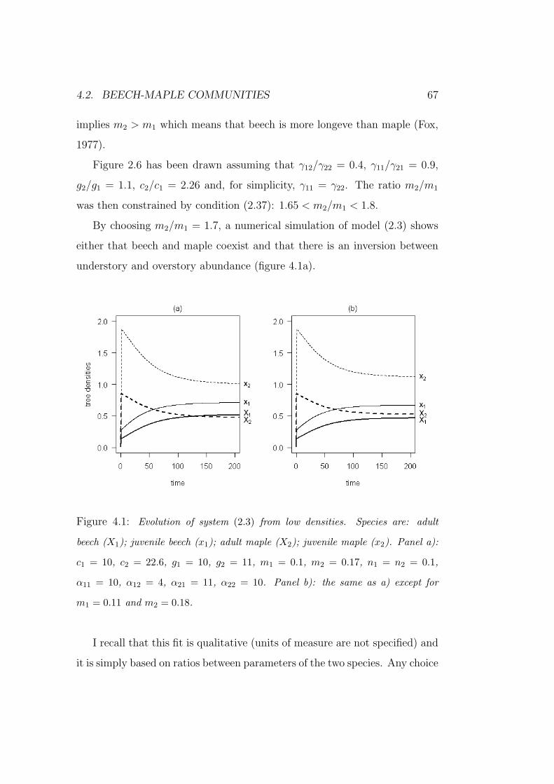
4.2. BEECH-MAPLE COMMUNITIES 67
implies m2 > m1 which means that beech is more longeve than maple (Fox,
1977).
Figure 2.6 has been drawn assuming that γ12/γ22 = 0.4, γ11/γ21 = 0.9,
g2/g1 = 1.1, c2/c1 = 2.26 and, for simplicity, γ11 = γ22. The ratio m2/m1
was then constrained by condition (2.37): 1.65 < m2/m1 < 1.8.
By choosing m2/m1 = 1.7, a numerical simulation of model (2.3) shows
either that beech and maple coexist and that there is an inversion between
understory and overstory abundance (figure 4.1a).
Figure 4.1: Evolution of system (2.3) from low densities. Species are: adult
beech (X1); juvenile beech (x1); adult maple (X2); juvenile maple (x2). Panel a):
c1 = 10, c2 = 22.6, g1 = 10, g2 = 11, m1 = 0.1, m2 = 0.17, n1 = n2 = 0.1,
α11 = 10, α12 = 4, α21 = 11, α22 = 10. Panel b): the same as a) except for
m1 = 0.11 and m2 = 0.18.
I recall that this fit is qualitative (units of measure are not specified) and
it is simply based on ratios between parameters of the two species. Any choice
68 CHAPTER 4. MODEL APPLICATIONS
of parameters in agreement with the ratios above, gives a similar qualitative
pattern.
Finally, the simple condition m2 > m1 is sufficient to reproduce the third
observation. I assumed that a windstorm kills a number of individuals of
each species in proportion to its relative abundance. Thus, I modelled the
windstorms by assuming that adult mortality of both species increase of an
amount δ (i.e., mi → mi + δ). Then, it is easy to show that:∣∣∣∣ d
dδ
(β1
β2
)∣∣∣∣δ=0
R 0 ifβ1
β2
Rc1g1m2
c2g2m1
m2
m1
. (4.1)
If the approximation (2.32) holds, equation (4.1) can be rewritten as:∣∣∣∣ d
dδ
(β1
β2
)∣∣∣∣δ=0
R 0 ifm2
m1
Q 1. (4.2)
This means that if species 1 has the highest longevity (i.e., m2/m1 > 1), then
raising the adult mortality of both species of an amount δ implies a decrease
of the ratio β1/β2, which in turn implies a decrease of the ratio X∗1/X
∗2 (see
figure 2.6).
Thus, model (2.3) predicts that an increase in tree-fall gaps, as a result
of an increase in windstorms, is followed by an increase of maple relative
abundance in the overstory. This is shown by the comparison between figure
4.1a (δ = 0) and figure 4.1b (δ = 0.01). From this point of view, coexistence
is the result of the internal structure of the system, while external variations
affect the equilibrium densities.
Forcier (1975) studied the dynamics of a beech-maple-birch community.
Beech and maple showed the same trade-off between strategies as in Poulson
and Platt (1996) and the yellow birch, that is too intolerant to establish
advanced reproduction in its own shade, persists because of its ability to
occupy recent openings (Forcier, 1975). This pattern can be interpreted
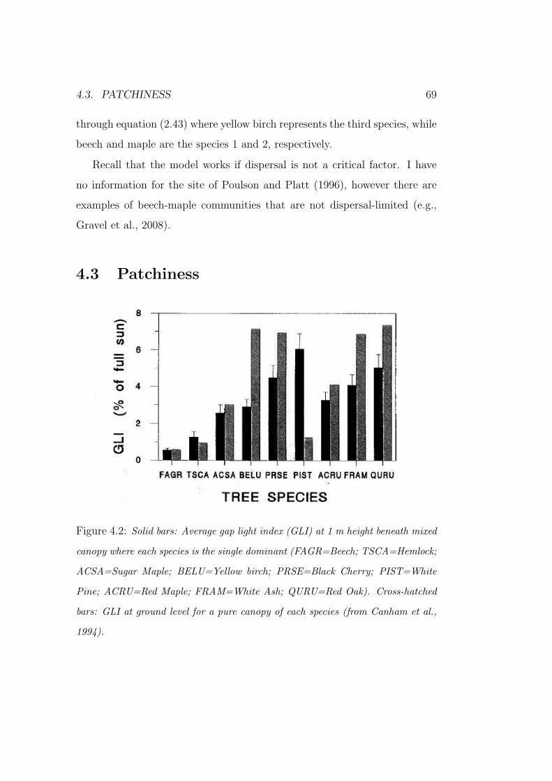
4.3. PATCHINESS 69
through equation (2.43) where yellow birch represents the third species, while
beech and maple are the species 1 and 2, respectively.
Recall that the model works if dispersal is not a critical factor. I have
no information for the site of Poulson and Platt (1996), however there are
examples of beech-maple communities that are not dispersal-limited (e.g.,
Gravel et al., 2008).
4.3 Patchiness
Figure 4.2: Solid bars: Average gap light index (GLI) at 1 m height beneath mixed
canopy where each species is the single dominant (FAGR=Beech; TSCA=Hemlock;
ACSA=Sugar Maple; BELU=Yellow birch; PRSE=Black Cherry; PIST=White
Pine; ACRU=Red Maple; FRAM=White Ash; QURU=Red Oak). Cross-hatched
bars: GLI at ground level for a pure canopy of each species (from Canham et al.,
1994).
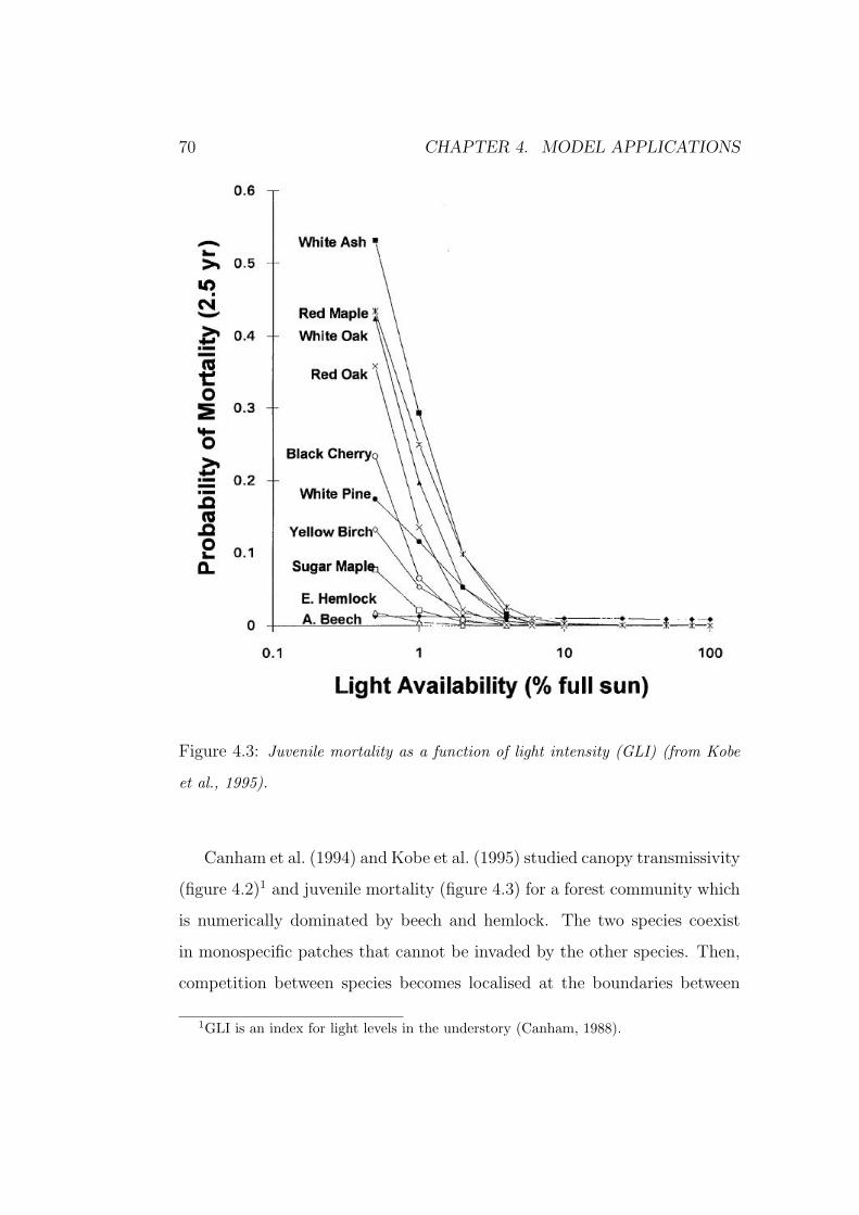
70 CHAPTER 4. MODEL APPLICATIONS
Figure 4.3: Juvenile mortality as a function of light intensity (GLI) (from Kobe
et al., 1995).
Canham et al. (1994) and Kobe et al. (1995) studied canopy transmissivity
(figure 4.2)1 and juvenile mortality (figure 4.3) for a forest community which
is numerically dominated by beech and hemlock. The two species coexist
in monospecific patches that cannot be invaded by the other species. Then,
competition between species becomes localised at the boundaries between
1GLI is an index for light levels in the understory (Canham, 1988).
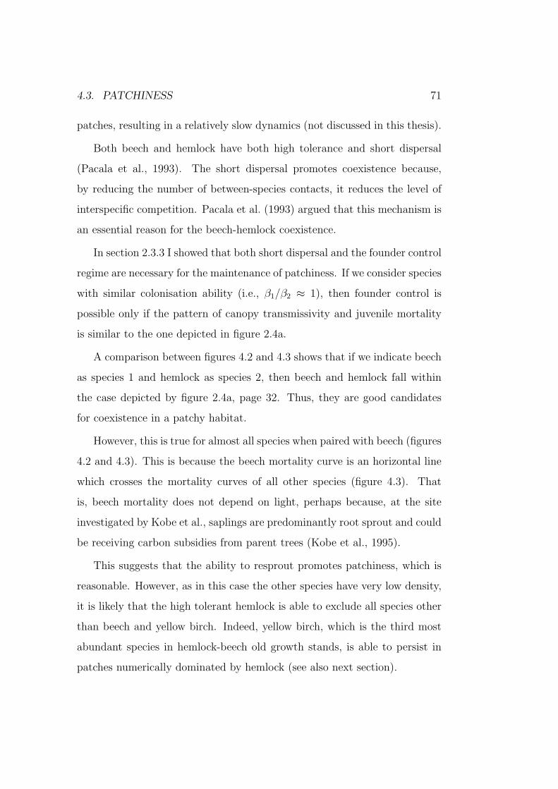
4.3. PATCHINESS 71
patches, resulting in a relatively slow dynamics (not discussed in this thesis).
Both beech and hemlock have both high tolerance and short dispersal
(Pacala et al., 1993). The short dispersal promotes coexistence because,
by reducing the number of between-species contacts, it reduces the level of
interspecific competition. Pacala et al. (1993) argued that this mechanism is
an essential reason for the beech-hemlock coexistence.
In section 2.3.3 I showed that both short dispersal and the founder control
regime are necessary for the maintenance of patchiness. If we consider species
with similar colonisation ability (i.e., β1/β2 ≈ 1), then founder control is
possible only if the pattern of canopy transmissivity and juvenile mortality
is similar to the one depicted in figure 2.4a.
A comparison between figures 4.2 and 4.3 shows that if we indicate beech
as species 1 and hemlock as species 2, then beech and hemlock fall within
the case depicted by figure 2.4a, page 32. Thus, they are good candidates
for coexistence in a patchy habitat.
However, this is true for almost all species when paired with beech (figures
4.2 and 4.3). This is because the beech mortality curve is an horizontal line
which crosses the mortality curves of all other species (figure 4.3). That
is, beech mortality does not depend on light, perhaps because, at the site
investigated by Kobe et al., saplings are predominantly root sprout and could
be receiving carbon subsidies from parent trees (Kobe et al., 1995).
This suggests that the ability to resprout promotes patchiness, which is
reasonable. However, as in this case the other species have very low density,
it is likely that the high tolerant hemlock is able to exclude all species other
than beech and yellow birch. Indeed, yellow birch, which is the third most
abundant species in hemlock-beech old growth stands, is able to persist in
patches numerically dominated by hemlock (see also next section).
72 CHAPTER 4. MODEL APPLICATIONS
4.4 Forest succession
Connell and Slatyer considered three conceptual models to describe succes-
sion. One of them, the inhibition model, is suitable for temperate forest.
It assumes that any arriving species, including those which usually appear
later, may be able to colonise. However, once earlier colonists secure the
space and/or other resources, they inhibit the invasion of subsequent colon-
ists or suppress the growth of those already present. The latter invade or grow
only when the dominating residents are damaged or killed, thus releasing re-
sources. The greater tolerance of late-succession species is of importance, not
in allowing net growth beneath earlier species, but in allowing the late species
to survive through long periods of suppression (Connell and Slatyer, 1977).
The model presented in this thesis (equations (2.3)) fully agrees with such
model. Indeed, the condition for a later species to invade an occupied habitat
is always more restrictive than the condition to invade an empty habitat (see
equation (2.8)). Moreover, later species can grow only when earlier species
release space (see equation (2.3a)), but they cannot displace earlier occupants
before they die (adult mortality does not depend on juvenile densities).
In order to highlight basic mechanisms behind succession, I now focus on
the additive version of model (2.3) (i.e., γi = γij = γik for every value of j
and k). In this case, a species always displaces the others (i.e., competitive
exclusion). Then, species i displaces species j if βi/γi > βj/γj (see condition
(2.17)). For each species it is convenient to define the competitive ability (or
competitiveness) ki as:
βi
γi
= ki. (4.3)
Then the higher the value of ki, the higher the competitive ability of species
i. In the unlikely case that more species have the same value of ki, those
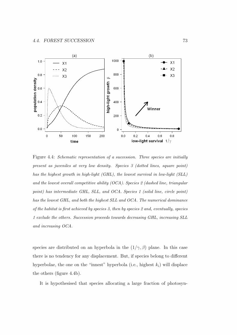
4.4. FOREST SUCCESSION 73
Figure 4.4: Schematic representation of a succession. Three species are initially
present as juveniles at very low density. Species 3 (dotted lines, square point)
has the highest growth in high-light (GHL), the lowest survival in low-light (SLL)
and the lowest overall competitive ability (OCA). Species 2 (dashed line, triangular
point) has intermediate GHL, SLL, and OCA. Species 1 (solid line, circle point)
has the lowest GHL, and both the highest SLL and OCA. The numerical dominance
of the habitat is first achieved by species 3, then by species 2 and, eventually, species
1 exclude the others. Succession proceeds towards decreasing GHL, increasing SLL
and increasing OCA.
species are distributed on an hyperbola in the (1/γ, β) plane. In this case
there is no tendency for any displacement. But, if species belong to different
hyperbolae, the one on the “innest” hyperbola (i.e., highest ki) will displace
the others (figure 4.4b).
It is hypothesised that species allocating a large fraction of photosyn-

74 CHAPTER 4. MODEL APPLICATIONS
thate to internal storage would have higher survival but would preclude car-
bohydrate allocation to rapid growth (Kobe, 1997). Thus, the competitive
ability of species is generally split into two strategies: opportunism (i.e.,
high growth in high-light, i.e., high βi) and tolerance (i.e., high survival in
low-light, i.e., high 1/γi).
Note that model (2.3) predicts that the “climax” species is that with the
highest value of ki irrespective of its strategy. If it is an opportunist species,
then we will not observe any succession.2 A succession occurs only when
the “climax” species is not the fastest invading species. That is, succession
proceeds towards increasing competitive ability, increasing tolerance level
and decreasing opportunism (figure 4.4). As we in fact observe successions,
it could be argued that the tolerance strategy is more effective than the
opportunist strategy in colonising a closed habitat.
Based on studies used for the parametrization of the forest simulator
SORTIE (Pacala et al., 1993), Pacala and colleagues identified the tree spe-
cies at their site according to both an index for high-light growth and an
index for low-light survival (figure 4.5) (Pacala et al., 1994; Kobe et al.,
1995). They interpreted figure 4.5 as if the species were arrayed along a
one-dimensional axis according to their successional status or, equivalently,
to their level of shade tolerance (successional status and shade tolerance are
closely related).
Species are traditionally classified into a roughly decreasing order of shade
tolerance as follows (Baker, 1949): beech, hemlock, sugar maple, red maple,
yellow birch, white pine, red oak, black cherry and white ash. Figure 4.5 has
2Here, I consider a situation where all possible species are present in the habitat at
some initial time. The generalization to the case where some species arrive later is straight-
forward.
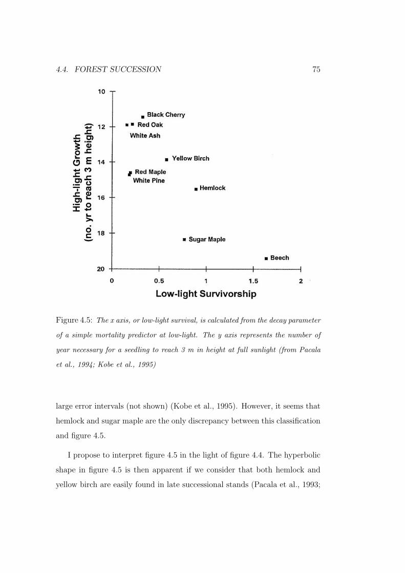
4.4. FOREST SUCCESSION 75
Figure 4.5: The x axis, or low-light survival, is calculated from the decay parameter
of a simple mortality predictor at low-light. The y axis represents the number of
year necessary for a seedling to reach 3 m in height at full sunlight (from Pacala
et al., 1994; Kobe et al., 1995)
large error intervals (not shown) (Kobe et al., 1995). However, it seems that
hemlock and sugar maple are the only discrepancy between this classification
and figure 4.5.
I propose to interpret figure 4.5 in the light of figure 4.4. The hyperbolic
shape in figure 4.5 is then apparent if we consider that both hemlock and
yellow birch are easily found in late successional stands (Pacala et al., 1993;
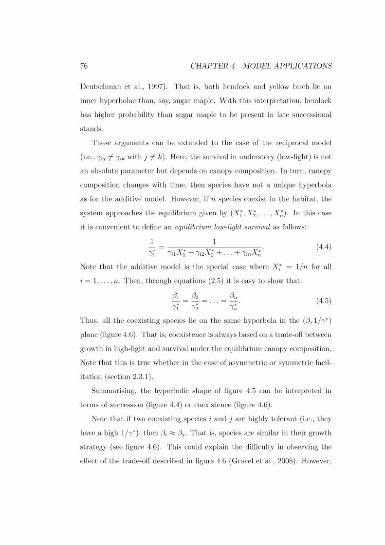
76 CHAPTER 4. MODEL APPLICATIONS
Deutschman et al., 1997). That is, both hemlock and yellow birch lie on
inner hyperbolae than, say, sugar maple. With this interpretation, hemlock
has higher probability than sugar maple to be present in late successional
stands.
These arguments can be extended to the case of the reciprocal model
(i.e., γij 6= γik with j 6= k). Here, the survival in understory (low-light) is not
an absolute parameter but depends on canopy composition. In turn, canopy
composition changes with time, then species have not a unique hyperbola
as for the additive model. However, if n species coexist in the habitat, the
system approaches the equilibrium given by (X∗1 , X
∗2 , . . . , X
∗n). In this case
it is convenient to define an equilibrium low-light survival as follows:
1
γ∗i=
1
γi1X∗1 + γi2X∗
2 + . . . + γinX∗n
. (4.4)
Note that the additive model is the special case where X∗i = 1/n for all
i = 1, . . . , n. Then, through equations (2.5) it is easy to show that:
β1
γ∗1=
β2
γ∗2= . . . =
βn
γ∗n. (4.5)
Thus, all the coexisting species lie on the same hyperbola in the (β, 1/γ∗)
plane (figure 4.6). That is, coexistence is always based on a trade-off between
growth in high-light and survival under the equilibrium canopy composition.
Note that this is true whether in the case of asymmetric or symmetric facil-
itation (section 2.3.1).
Summarising, the hyperbolic shape of figure 4.5 can be interpreted in
terms of succession (figure 4.4) or coexistence (figure 4.6).
Note that if two coexisting species i and j are highly tolerant (i.e., they
have a high 1/γ∗), then βi ≈ βj. That is, species are similar in their growth
strategy (see figure 4.6). This could explain the difficulty in observing the
effect of the trade-off described in figure 4.6 (Gravel et al., 2008). However,
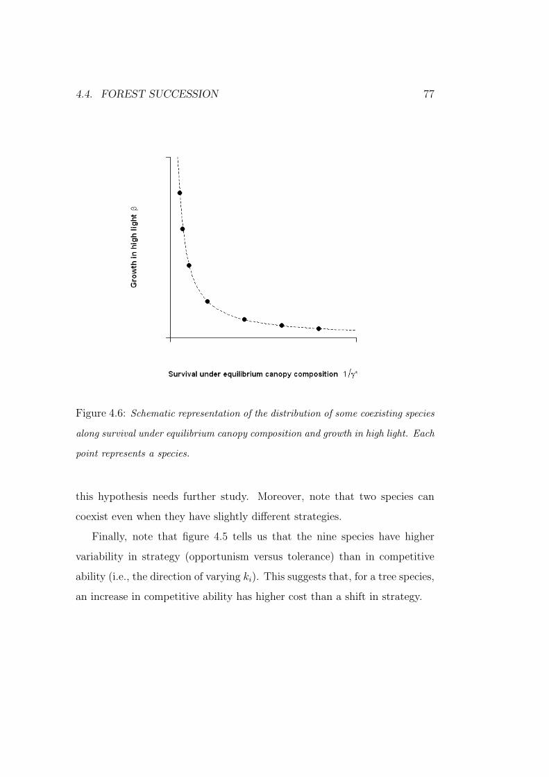
4.4. FOREST SUCCESSION 77
Figure 4.6: Schematic representation of the distribution of some coexisting species
along survival under equilibrium canopy composition and growth in high light. Each
point represents a species.
this hypothesis needs further study. Moreover, note that two species can
coexist even when they have slightly different strategies.
Finally, note that figure 4.5 tells us that the nine species have higher
variability in strategy (opportunism versus tolerance) than in competitive
ability (i.e., the direction of varying ki). This suggests that, for a tree species,
an increase in competitive ability has higher cost than a shift in strategy.

78 CHAPTER 4. MODEL APPLICATIONS
Chapter 5
Concluding remarks
5.1 Model structure
Many competition models belong to the Lotka-Volterra type. Such models
have been criticised because their level of abstraction makes them fundament-
ally disconnected from life-history parameters that can be measured in the
field. A different approach is based on the von-Foerster equation (see section
3.5). In this case, model parameters are clearly linked to measurable indi-
vidual tree attributes such as growth and mortality (Kohyama, 1992, 1993;
Kohyama et al., 2001; Hurtt et al., 1998; Moorcroft et al., 2001; Kohyama,
2005). Generally, this second type of models has to be solved numerically,
thus complicating the analysis.
The model developed in this thesis can be considered as a compromise
between these two mathematical approaches: the model is completely tract-
able (as for the usual Lotka-Volterra equations) but it is mechanistically
based on life-history parameters (as for the von Foerster type of models).
The structure of the model is very simple: just two stage levels and yet it
can explain many observed behaviours (see section 2.3.1). Thus, the main
79
80 CHAPTER 5. CONCLUDING REMARKS
merit of this model is its simplicity which in turn allows an understanding of
mechanisms behind forest dynamics. Note that when the von-Foerster model
is simplified to a two-stage model (Adams et al., 2007), the predictions of the
two approaches are similar, even if the von-Foerster model lacks an explicit
description of density dependence (see section 3.5).
This simplicity was possible because I assumed that populations are well
mixed. Thus, I neglected possible effects associated with explicit spatial pat-
terns by using the simple mean field approximation (Klausmeir and Tilman,
2002). Spatial patterns can be unequivocally important (e.g., Gilad et al.,
2007), also they can be studied with analytical techniques (e.g., Bolker and
Pacala, 1997, 1999). However, some interesting features are predicted even
in this simple case and I believe that is worth showing these results before
using more sophisticated techniques.
The present model describes the dynamics of n species competing for
space. The space in turn mediates for light and other resources. Competi-
tion for space follows the basic idea of gap dynamics (Watt, 1947): a forest
is a mosaic of tree crowns (i.e., cells). The individual trees that are the ele-
ments of this mosaic dominate the resources and block the growth of young
trees. When they die and open a gap in the canopy, a number of responses
are initiated in the small area below the canopy opening. These responses
eventually lead to the repair of the forest canopy. The importance of gap dy-
namics within the overall forest dynamics is widely recognised (e.g., Canham,
1989; McCarthy, 2001).
The real gap dynamics is often more complex than the simple description
above. For example, in beech-maple communities, saplings experience several
periods of suppression and release before attaining the canopy (Canham,
1990) and the gap size could be important (Poulson and Platt, 1996; Runkle,
5.1. MODEL STRUCTURE 81
1982; Kohyama, 1984). However, these and other mechanisms have been
sacrificed for the sake of simplicity.
Once a plant attains the canopy, it does not suffer competition for re-
sources any more. Thus, adult mortality is density independent (I implicitly
considered as adult, only those trees that survive self-thinning). On the other
hand, adults significatively modify the juvenile microenvironment, then ju-
venile mortality is density dependent. Moreover, I assumed that juvenile
mortality only depends on adult density i.e., juveniles do not interfere with
each other in the use of resources. This assumption both simplify the equa-
tions and is ecologically reasonable. Indeed, often light is the most limiting
resource for sapling growth (Canham et al., 1994; Pacala et al., 1994) and
most of shade is cast by adults. Clearly, the assumption that juveniles do
not inhibit each other holds for relatively low densities of suppressed plants.
This hypothesis of reduced competition has been analysed as an explanation
for biodiversity in tropical forests (Wright, 2002).
Because of mortality, adult trees cannot completely fill the habitat (see
equations (2.12), (2.14), (2.15)). Then, a number of gaps is always present.
However, tree crowns tend to cover the full space in the limit of low adult
mortality (i.e., when β →∞). In general, this is possible if tree crowns have
plastic growth. Then, the portion of occupied space is computed through
the mean crown area (si) times the number of adult trees (Pi) (see equations
(2.2)).
I assumed that the mean crown area is a species-specific parameter even if,
in principle, it could be density dependent. There is a clear link between the
mean crown area of the present model and the threshold size of the model of
Adams et al. (2007) discussed in section 3.5 (see also Strigul et al., 2008). In
their model, the threshold size between understory and overstory is a dynamic

82 CHAPTER 5. CONCLUDING REMARKS
variable. However, both models lead to conceptually identical conditions for
the equilibrium behaviours of a two species system (see section 3.5). So, in
order to study equilibrium dynamics, the approximation of constant mean
crown area is not restrictive.
The interaction between adults and juveniles is modelled through the α
coefficients. If shade is the main effect, then they represent a compound
measure of shade cast by adults and shade tolerance of juveniles (see section
2.3.1). But other effects could be important e.g., root competition, allel-
opathy and pest facilitation (see a review in Wright, 2002). Then, the α
coefficients should be considered as composed by several components:
αij = αlightij + αroot
ij + αallij + αpest
ij + . . . . (5.1)
In the model presented in this thesis, coexistence is represented as a stable
equilibrium point of the system (deterministic model). A different approach
is to consider a periodically perturbated system. Such perturbations (e.g.,
fires, windstorms) could lead to a nonequilibrium coexistence even if the un-
perturbed system could not (Huston, 1979). In the ecological literature there
is debate on which is the better explanation for coexistence, indeed natural
system are always perturbed (DeAngelis and Waterhouse, 1987). However,
external perturbations promote nonequilibrium coexistence only if they have
suitable magnitude and frequency. On the other hand, in a deterministic
model, small perturbations often keep the system slightly away from the
equilibrium. In the latter case we have a slightly perturbed equilibrium co-
existence. Indeed, this is the case for the model presented in this thesis: small
random perturbations can be easily added to the system. They produce some
noise on curves in figure 4.1 at page 67 but the pattern is unchanged (not
shown).
5.2. MODEL RESULTS 83
5.2 Model results
The basic structure of the model presented in this thesis (equations (2.3)) can
be summarized in five points: (i) trees are classified in two stage levels (ii) all
adult trees are exposed to full light and cannot be dislodged by juveniles; (iii)
juvenile trees can grow only when adult trees die, thus releasing space; (iv)
adult trees affect juvenile survival; (v) only adult trees can reproduce. Essen-
tially, this is the “inhibition model” of succession proposed by Connell and
Slatyer (1977). Moreover, it captures the essence of gap dynamics as well.
All model results are consequences of these five statements. Although the
model has not been validated, I have performed several qualitative comparis-
ons with studies from literature that support the model results. Furthermore,
the model provides possible explanations for the observed patterns.
When only one species is considered the most interesting prediction is that
both the light transmissivity of canopy trees and the tolerance of juveniles do
not affect the ability to invade a habitat. On the other hand, they affect the
equilibrium density in a way that monocultures of tolerant species are denser
than monoculture of intollerant species even if they have the same ability to
colonise an empty habitat. This is widely observed in nature (Horn, 1971).
When two species are considered, three behaviours are possible: coexist-
ence, founder control and competitive exclusion. Then, the simple two-stage
structure allows for coexistence, but only if the one-sided effects of adult trees
on juvenile trees are species-specific. This agrees with the finding of Canham
et al. (1994) and Pacala et al. (1993) on the importance of species-specific
traits in canopy attributes. Note that this result holds for any functional
form of juvenile mortality.
Two species can coexist in two cases. First, if the juveniles of both species
are more inhibited by conspecific adults than by heterospecific adults. This

84 CHAPTER 5. CONCLUDING REMARKS
pattern leads to the reciprocal replacement that has been observed in many
beech-maple communities (Fox, 1977; Woods, 1979; Chyper and Boucher,
1982). Secondly, coexistence could be based on a trade-off between toler-
ance and growth ability. This pattern has also been observed in beech-maple
communities (Forcier, 1975; Canham, 1989; Poulson and Platt, 1996). In
particular, Poulson and Platt (1996) hypothesised that coexistence was pro-
moted by a change in adult mortality as a result of increased windstorms. A
qualitative comparison between the model and the study of Poulson and Platt
showed that coexistence could be based on the internal structure alone, while
the external forcing affects the relative abundances. Moreover, in both cases
mentioned above, the maintenance of the co-dominance is always based on a
trade-off between growth and survival under the equilibrium canopy compos-
ition. The coexisting species are then distributed along these two strategies
in a pattern similar to the one found by Kobe et al. (1995). Note that even
a slight difference between these two strategies could result in coexistence,
thus explaining coexistence of highly tolerant tree species.
In contrast with the simple Lotka-Volterra models, here the juvenile stage
is considered explicitly. This allows us to know the abundances of both
adults and juveniles. This is useful to compare equilibrium abundances of
the two stages. For example, analysing several natural forests in North Amer-
ica which are numerically dominated by two species, Fox (1977) found that
the species with highest longevity is generally more abundant in the over-
story, while the other species is generally more abundant in the understory.
Moreover, Fox pointed out that this is not obviously explained by seed year
frequency, seed size or seed number. In particular, in the beech-maple com-
munity studied by Poulson and Platt, maple has smaller abundance in the
overstory and higher abundance in the understory and this pattern seems to
5.2. MODEL RESULTS 85
be a stable feature of the system (Poulson and Platt, 1996). It is possible to
define a range in the model parameters that leads to this pattern irrespective
of the relative magnitude of fecundity parameters for the two species. Thus,
the inversion of abundances can be interpreted as an internal feature of the
system: within the pattern of reciprocal replacement, individuals leave the
juvenile class either by growth or death. Thus, juveniles that generally re-
place the shorter-lived species, are expected to have lesser abundance in the
understory.
Within the model presented in this thesis, competitiveness of each species
has two key components or strategies: the ability to grow when space is avail-
able (growth in high-light) and the ability to survive under a given canopy
(survival in low-light). The most important feature of the model is that the
low-light survival depends on the canopy composition. This is the key for the
coexistence (reciprocal model). However, in the simple case where all canopy
trees have the same light transmissivity, the low-light survival is an absolute
species-specific parameter. In this case, the species with the highest compet-
itiveness outcompete the others irrespective of their strategies. Moreover, if
few juveniles of two species are present in a habitat at some initial time, we
observe a succession only if the species with the highest competitiveness is the
species with both the highest survival in low-light and the smallest growth
in high-light. This suggests that we should interpret growth in high-light
and survival in low-light as the two components of the successional status as
well. Then, successions proceed towards increasing competitiveness, increas-
ing survival in low-light and decreasing growth in high-light.
Successional status and shade tolerance are often considered as equivalent
concepts (Horn, 1971; Kobe et al., 1995). In contrast, I considered the shade
tolerance equivalent to survival in low-light. Note that this sets a subtle but
86 CHAPTER 5. CONCLUDING REMARKS
profound difference between successional status and shade tolerance. For
example, sugar maple could have a higher competitiveness than beech even
though beech is more tolerant than maple, in this case maple could outcom-
pete beech, thus having a higher successional status. Thus, when species are
distributed along the two strategies (see Kobe et al., 1995) we have a better
understanding of their successional status if both the overall competitiveness
and the shade tolerance are considered as the drivers of the succession.
The model presented in this thesis is based on a mean-field approximation.
This means that the model does not deal with the spatial distribution of
species. However, some spatial information can be inferred. Indeed, in the
case of founder control, several species could persist in a patchy habitat
(Yodzis, 1978; Shmida and Ellner, 1984). A comparison of the model with
the juvenile mortality curves found by Kobe et al. (1995) suggests that beech
has a tendency to persist in patches. This is because beech saplings are
predominantly root sprout at the site of Kobe et al.. Indeed, typically beech
and hemlock coexist in a patchy habitat.
For many years competition was thought to play a predominant role in
structuring plant communities. However, facilitation effects are now receiving
a growing attention (Holmgren et al., 1997; Bruno et al., 2003). In the model
presented in this thesis some degree of relative interspecific facilitation is a
critical component for coexistence. Moreover, note that in principle, the
αij coefficients could be negative indicating an absolute facilitation. Even
in the latter case, species coexist in a pattern qualitatively described by
figure 2.3d (page 30). Then, when the two species approach the equilibrium,
one increases while the other decreases. This implies an overall competitive
interaction (Pielou, 1977; Kot, 2003).
Thus, even if facilitative interactions between life stages play a critical role

5.2. MODEL RESULTS 87
in structuring the community, they are always overridden by the competition
for the space. This is also evident because according to the inhibition model
of succession of Connell and Slatyer (1977), the condition to invade an empty
habitat is always less restrictive than the condition to invade an occupied one
(see equation (2.16)).
I view the present model as a step towards a comprehensive understand-
ing of interspecific competition in forest ecosystems. Its merit is to provide
a simple vision on the importance of interactions between life stages in ex-
plaining coexistence.

88 CHAPTER 5. CONCLUDING REMARKS
Bibliography
Adams, T. P., Purves, D. W., and Pacala, S. W. (2007). Understanding
height-structured competition in forests: is there an R* for light? Pro-
ceedings of the Royal Society B, 274:3039–3047.
Baker, F. S. (1949). A revised tolerance table. Journal of Forestry, 47:179–
181.
Bazzaz, F. A. (1979). The physiological ecology of plant succession. Annual
Review of Ecology, Evolution and Systematics, 10:351–372.
Bolker, B. M. and Pacala, S. W. (1997). Using moment equations to under-
stand stochastically driven spatial patterns formation in ecological systems.
Theoretical Population Biology, 52:179–197.
Bolker, B. M. and Pacala, S. W. (1999). Spatial moment equations for plant
competition: understanding spatial strategies and the advantages of short
dispersal. American Naturalist, 153:575–602.
Botkin, D. B., Janak, J. F., and Wallis, J. R. (1972). Rationale, limitations,
and assumptions of a northeastern forest growth simulator. IBM Journal
of Research and Development, 16:106–116.
Bruno, J. F., Stachowicz, J. J., and Bertness, M. D. (2003). Inclusion of
89
90 BIBLIOGRAPHY
facilitation into ecological theory. Trends in Ecology and Evolution, 18:119–
125.
Bugmann, H. (2001). A review of forest gap models. Climatic Change,
51:259–305.
Canham, C. D. (1988). An index for understory light levels in and around
canopy gaps. Ecology, 69:1634–1638.
Canham, C. D. (1989). Different responces to gaps among shade-tollerant
tree species. Ecology, 70:548–550.
Canham, C. D. (1990). Suppression and release during canopy recruitment
of Acer saccharum and Fagus grandifolia. Bulletin of the Torrey Botanical
Club, 117:1–7.
Canham, C. D., Finzi, A. C., Pacala, S. W., and Burbank, D. H. (1994).
Causes and consequences of resource heterogeneity in forests: Interspecific
variation in light transmission by canopy trees. Canadian Journal of Forest
Reserch, 24:337–349.
Chesson, P. (2000). Mechanisms of manteinance of species diversity. Annual
Review of Ecology and Systematics, 31:343–366.
Chyper, J. and Boucher, D. H. (1982). Beech-maple coexistence and seedling
growth rates at Mont-Saint-Hilaire, quebec. Canadian Journal of Botany,
60:1279–1281.
Connell, J. H. and Slatyer, R. O. (1977). Mechanisms of succession in nat-
ural communities and their role in community stability and organization.
American Naturalist, 111:1119–1144.

BIBLIOGRAPHY 91
Cramer, W., Bondeau, A., Woodward, F. I., Prentice, I. C., Betts, R. A.,
Brovkin, V., Cox, P. M., Fisher, V., Foley, J. A., Friend, A. D., Kucharik,
C., Lomas, M. R., Ramankutty, N., Sitch, S., Smith, B., White, A., and
Young-Molling, C. (2001). Global responce of terrestrial ecosystem struc-
ture and function to CO2 and climatic change: results from six dynamic
global vegetation models. Global Change Biology, 7:357–373.
Davis, A. J., Jenkinson, L. S., Shorrocks, B., and Wood, S. (1998). Mak-
ing mistakes when predicting shifts in species range in response to global
warming. Nature, 391:783–786.
DeAngelis, D. L. and Waterhouse, J. C. (1987). Equilibrium and nonequi-
librium concepts in ecological models. Ecological Monographs, 57:1–21.
Deutschman, D. H., Levin, S. A., Devine, C., and Buttel, L. A. (1997).
Scaling from trees to forests: Analysis of a complex simulation model.
Science Online.
Forcier, L. K. (1975). Reproductive strategies and the co-occurence of climax
tree species. Science, 189:808–810.
Fox, J. F. (1977). Alternation and coexistence of tree species. American
Naturalist, 111:69–89.
Friedlingstein, P., Cox, P., Betts, R., Bopp, L., von Bloh, W., Brovkin, V.,
Cadule, P., Doney, S., Eby, M., Fung, I., Bala, G., John, J., Jones, C.,
Joos, F., Kato, T., Kawamiya, M., Knorr, W., Lindsay, K., Matthews,
H. D., Raddatz, T., Rayner, P., Reick, C., Roec, E., Schnitzler, K.-G.,
Schnur, R., Strassmann, K., Weaver, A. J., Yoshikawa, C., and Zeng, N.
(1996). Climate-carbon cycle feedback analysis: Results from the C4MIP
model intercomparison. Journal of Vegetation Science, 19:3337–3353.
92 BIBLIOGRAPHY
Gilad, E., von Hardenberg, J., Provenzale, A., Shachak, M., and Meron, E.
(2007). A mathematical model of plants as ecosystem engineers. Journal
of Theoretical Biology, 244:680–691.
Gravel, D., Beaudet, M., and Messier, C. (2008). Partitioning the factors
of spatial variation in regeneration density of shade-tolerant tree species.
Ecology, 89:2879–2888.
Hardin, G. (1960). The competitive exclusion principle. Science, 131:1292–
1297.
Holmgren, M., Sheffer, M., and Huston, M. A. (1997). The interplay of
facilitation and competition in plant communities. Ecology, 78:1966–1975.
Horn, H. S. (1971). The Adaptive Geometry of Trees. Princeton University
Press.
Huisman, J. and Weissing, F. J. (2001). Biological conditions for oscillations
and chaos generated by multispecies competition. Ecology, 82:2682–2695.
Hurtt, G. C., Moorcroft, P. R., and Pacala, S. W. (1998). Terrestrial model
and global change: challenge for the future. Global Change Biology, 4:581–
590.
Huston, M. (1979). A general hypothesis of species diversity. The American
Naturalist, 113:81–101.
Hutson, V. and Law, R. (1985). Permanent coexistence in general models of
three interacting species. Journal of Mathematical Biology, 21:285–298.
Kelly, C. K. and Bowler, M. G. (2002). Coexistence and relative abundance
in forest trees. Nature, 417:437–440.
BIBLIOGRAPHY 93
Klausmeir, C. and Tilman, D. (2002). Competition and coexistence. In Som-
mers, U. and Worm, B., editors, Ecological Studies, volume 161. Springer-
Verlag Berlin Heidelberg.
Kobe, R. K. (1997). Carbohydrate allocation to storage as a basis of inter-
specific variation in sapling survivorship and growth. Oikos, 80:226–233.
Kobe, R. K., Pacala, S. W., Silander, J. A., and Canham, C. D. (1995).
Juvenile tree survivorship as a component of shade tolerance. Ecological
Applications, 5:517–532.
Kohyama, T. (1984). Regeneration and coexistence of two Abies species
dominating subalpine forests in central japan. Oecologia, 62:156–161.
Kohyama, T. (1992). Size-structured multi-species model of rain forest trees.
Functional Ecology, 6:206–212.
Kohyama, T. (1993). Size-structured tree populations in gap-dynamic forest
– the forest architecture hypothesis for the stable coexistence of species.
Journal of Ecology, 81:131–143.
Kohyama, T. (2005). Scaling-up from shifting-gap mosaic to geographic dis-
tribution in the modelling of forest dynamics. Ecological Research, 20:305–
312.
Kohyama, T., Suzuki, E., Partomihardjo, T., and Yamada, T. (2001). Dy-
namic steady state of patch-mosaic tree size structure of a mixed diptero-
carp forest regulated by local crowding. Ecological Research, 16:85–98.
Kohyama, T. and Takada, T. (2009). The stratification theory for plant co-
existence promoted by one-sided competition. Journal of Ecology, 97:463–
471.
94 BIBLIOGRAPHY
Kot, M. (2003). Elements of Mathematical Ecology. Cambridge University
Press.
Levins, R. (1969). Some demographic and genetic consequences of environ-
mental heterogeneity for biological control. Bullettin of the Entomological
Society of America, 15:237–240.
Lotka, A. J. (1932). The growth of mixed populations, two species compet-
ing for a common food supply. Journal of the Washington Academy of
Sciences, 22:461–469.
McCarthy, J. (2001). Gap dynamics of forest trees: A review with particular
attention to boreal forests. Environmental Review, 9:1–59.
Moorcroft, P. R., Hurtt, G. C., and Pacala, S. W. (2001). A method for scal-
ing vegetation dynamics: the ecosystem demography model (ED). Ecolo-
gical Monographs, 71:557–586.
Nakashizuka, T. and Kohyama, T. (1995). The significance of asymmetric
effect of crowding for coexistence in a mixed temperate forest. Journal of
Vegetation Science, 6:509–516.
Pacala, S. W., Canham, C. D., and Silander, J. A. (1993). Forest mod-
els defined by field measurements: I. the design of a north-eastern forest
simulator. Canadian Journal of Forest Reserch, 23:1980–1988.
Pacala, S. W., Canham, C. D., Silander, J. A., and Kobe, R. K. (1994).
Sapling growth as a function of resources in a north temperate forest.
Canadian Journal of Forest Reserch, 24:2172–2183.
Pacala, S. W. and Tilman, D. (1994). Limiting similarity in mechanistic
BIBLIOGRAPHY 95
and spatial models of plant competition in heterogeneous environments.
American Naturalist, 143:222–257.
Pearson, R. G. and Dawson, T. P. (2003). Predicting the impacts of climate
change on the distribution of species: are bioclimate envelope models use-
ful? Global Ecology and Biogeography, 12:361–371.
Peng, C. (2000). From static biogeographical model to dynamic global ve-
getation model: a global perspective on modelling vegetation dynamics.
Ecological Modelling, 135:33–54.
Pielou, E. C. (1977). Mathematical Ecology. John Wiley & Sons, Inc.
Poulson, T. L. and Platt, W. J. (1996). Replacement patterns of beech and
sugar maple in Warren Woods, Michigan. Ecology, 77:1234–1253.
Prentice, I. and GVDM Members (1989). Developing a global vegetation
dynamics model: results of an IIASA summer workshop. RR-89-7, Lax-
enburg, Austria. International Institute for Applied Systems Analysis (II-
ASA).
Purves, D. and Pacala, S. W. (2008). Predictive models of forest dynamics.
Science, 320:1452–1453.
Runkle, J. R. (1982). Pattern of disturbance in some old-growth mesic forests
of eastern North America. Ecology, 63:1533–1546.
Shmida, A. and Ellner, S. (1984). Coexistence of plant species with similar
niches. Vegetatio, 58:29–55.
Silvertown, J. (2004). Plant coexistence and the niche. Trends in Ecology
and Evolution, 19:605–611.

96 BIBLIOGRAPHY
Steffen, W., Cramer, W., Plochl, M., and Bugmann, H. (1996). Global
vegetation models: incorporating transient changes to structure and com-
position. Journal of Vegetation Science, 7:321–328.
Steffen, W. L., Walker, B. H., Ingram, J. S. I., and Koch, G. W. (1992).
Global change and terrestrial ecosystems: the operational plan. Technical
Report 21, IGBP, The Royal Swedish Academy of Sciences, Stockholm,
Sweden.
Strigul, N., Pristinsky, D., Purves, D. W., Dushoff, J., and Pacala, S. W.
(2008). Scaling from trees to forest: tractable macroscopic equations for
forest dynamics. Ecological Monographs, 78:523–545.
Taneyhill, D. E. (2000). Metapopulation dynamics of multiple species: the
geometry of competition in a fragmented habitat. Ecological Monograph,
70:495–516.
Thuiller, W. (2003). BIOMOD – optimizing predictions of species distribu-
tions and projecting potential future shifts under global change. Global
Change Biology, 9:1353–1362.
Tilman, D. (1994). Competition and biodiversity in spatially structured
habitats. Ecology, 75:2–16.
Tilman, D. and Wedin, D. (1991). Dynamics of nitrogen competition between
successional grasses. Ecology, 72:1038–1049.
United Nations Framework Convention on Climate Change (1997). Kyoto
Protocol to the United Nations Framework Convention on Climate Change.
volume 24, UN, Geneve.
BIBLIOGRAPHY 97
U.S. Department of Agriculture (1974). Seeds of woody plants in the United
States. U.S. Department of Agriculture, Agriculture Handbook 450 Wash-
ington, DC.
Valladares, F. and Niinemets, U. (2008). Shade tolerance, a key plant feature
of complex nature and consequences. Annual Review of Ecology, Evolution
and Systematics, 39:237–257.
Vance, R. R. (1984). Interference competition and the coexistence of two
competitors on a single limiting resource. Ecology, 65:1349–1357.
Volterra, V. (1926). Fluctuation in the abundance of a species considered
mathematically. Nature, 118:558–560.
Watt, A. S. (1947). Pattern and process in the plant community. Journal of
Ecology, 35:1–22.
Whittaker, R. H. and Levin, S. A. (1977). The role of mosaic phenomena in
natural communities. Theoretical Population Biology, 12:117–139.
Woods, K. D. (1979). Reciprocal replacement and the manteinance of codom-
inance in a beech-maple forest. Oikos, 33:31–39.
Woodward, F. I. (1987). Climate and Plant Distribution. Cambridge Uni-
versity Press.
Wright, S. J. (2002). Plant diversity in tropical forests: a review of mechan-
isms of species coexistence. Oecologia, 130:1–14.
Yodzis, P. (1978). Competition for Space and the Structure of Ecological Com-
munities. Lecture Notes in Biomathematics 25. Springer-Verlag, Berlin-
Heidelberg-New York.