genetic and taxonomic incongruences in mediterranean...
TRANSCRIPT
UNIVERSITÀ DEGLI STUDI DELLA TUSCIA DI VITERBO
DIPARTIMENTO DI SCIENZE E TECNOLOGIE PER L'AGRICOLT URA, LE FORESTE, LA NATURA E L'ENERGIA (DAFNE)
Corso di Dottorato di Ricerca in
Scienze e tecnologie per la gestione forestale e ambientale - XXV Ciclo.
Genetic and taxonomic incongruences in Mediterranean endemic flora: four different case studies
s.s.d. AGR/05
Tesi di dottorato di:
Dott. Tamara Kirin
Coordinatore del corso Tutore
Prof. Rosanna Bellarosa Prof. Bartolomeo Schirone
7 Maggio 2013
Preface
PREFACE
The Mediterranean Basin is a region of great biodiversity. Around 10% of all the existing
plant species in the world inhabit this small area. This amazing fact provides opportunities
for continuous botanical studies and analyses. Long and complex geological history and
long-term climate of the Mediterranean offer a vast number of particular microhabitats
inhabited by isolated, highly specialised species and subspecies. High genetic richness
appears to be another particularity of the area which is still being recognised and
investigated.
This is why I decided to study genetic variation of four different Mediterranean species
complexes. The selected species include herbaceous and woody taxa, as well as
Gymnosperms and Angiosperms. European Black Pine (Pinus nigra Arnold.) and Aleppo
Pine (Pinus halepensis Mill.), ancient gymnosperms, represent two of the core species of
the Mediterranean. Despite similarly high importance in habitats they occupy, areas which
they inhabit are very different, resulting in different ecology and life-history traits of these
two species. European Nettle Tree (Celtis australis L.), though not exclusively a
Mediterranean species, represents an important element of the Mediterranean vegetation
and has had an important role for the local inhabitants, from the time of the first settlers till
today (alimentary, wood, spiritual and horticultural). Its particularities are also two closely
related species (C. tournifortii Lam. and, so called, C. aethnensis (Tornab.) Strobl) with
their unresolved phylogenetic status. The last of the studied taxa is an herbaceous group of
plants, Inula verbascifolia group, which represents a complex of strictly Mediterranean
plants from which I restricted my analyses on Inulas verbascifolia subsp. verbascifolia
taxa. The centre of their distribution is the Ionic Sea and their divergence in an outcome of
particular environmental conditions around the Mediterranean costs.
I this work I analyzed intra-specific genetic diversity and phylogeography of four species,
in order to resolve the existing incongruence in their systematics. By applying various
molecular methods and testing various regions of the genome I aimed to provide a

Preface
comprehensive molecular systematics of the studied species to help and encourage various
future studies. Moreover, I applied the same approach in computational genetic analyses,
testing different methods and models. I discuss, both, the results and the applicability of all
the applied methods. Finally, I introduced a brand new technology called High resolution
melting (HRM) to test and, eventually recommend its use, in phylogenetics and
phylogeography studies, fields in which it has never been used before.
Apart from giving new insights to the phylogenetics of the studied groups, I hope this
study will provide an overview of the present molecular techniques and encourage more
studies on unresolved evolutionary traits in Mediterranean Basin. At the end, we should
never forget the biodiversity loss we are experiencing at the moment. The biodiversity
should not be regarded only at the level of species but also on the genetic level. Therefore
any study on genetic variability is also a study towards the conservation of some unique
identities.
Table of Contents
TABLE OF CONTENTS
1. INTRODUCTION …………………………………………………………………… 1
1.1. Mediterranean region ……………………………………………………….. 1
1.1.1. Mediterranean Basin and its biodiversity ………………...………. 3
1.1.2. Geology and history of the Mediterranean region …….…………... 4
1.1.3. Pleistocene in the Mediterranean region …………….,…………… 5
1.1.4. Evolution after the Pleistocene and human impact
on the vegetation ………………………………………………………… 7
1.2. Studied species ……………………………………………………………… 9
1.2.1. Genus Pinus ……………………………………………………….. 9
1.2.1.1. Evolution of pines ……………………………………….. 9
1.2.1.2. Pines of the Mediterranean Basin ……………………….. 10
1.2.1.3. Genetic diversity of pines ………………………………. 11
1.2.1.4. Systematics of genus Pinus ................................................ 12
1.2.1.5. Aleppo pine (Pinus halepensis Miller) .............................. 13
1.2.1.6. European black pine (Pinus nigra Arnold)......................... 18
1.2.2. Genus Celtis ……………………………………………………….. 27
1.2.2.1. European nettle tree (Celtis australis L.) ……………….. 28
1.2.2.2. Oriental Hackberry (Celtis tournefortii Lam.) …………... 29
1.2.3. Inula verbascifolia subsp. verbascifolia … ………………………. 29
1.3. Molecular analyses ………………………………………………………….. 32
1.3.1. Discovering the variability and evolutionary

Table of Contents
history of the species ……………………………………............... 33
1.3.2. Molecular markers used for DNA sequencing …………………….. 36
1.3.3. Molecular phylogenetics ................................................................... 44
2. OBJECTIVES AND SCOPE OF THE STUDY ……………………………………… 50
3. MATERIAL AND METHODS ………………………………………………………. 52
3.1. Sampling ……………………………………………………………………. 52
3.2. Conserving the material ……………………………………………………... 58
3.3 DNA extraction ……………………………………………………………..... 59
3.4. Amplification of the fragment using the PCR machine ……………………. 62
3.5. DNA purification ……………………………………………………………. 64
3.6. DNA fragments verification – Gel electrophoresis ………………………… 65
3.7. DNA sequencing ……………………………………………………………. 66
3.8. Bioinformatics ………………………………………………………………. 66
3.8.1. Chromatogram visualization ………………………………………. 66
3.8.2. Multiple sequence alignment ……………………………………… 67
3.8.3. Mesquite 2.75. …………………………………………………….. 67
3.8.4. DnaSP 5.10. ……………………………………………………….. 68
3.8.5. Mega 5.0. ………………………………………………………...... 68
3.8.6. RAxML ……………………………………………………………. 69
3.8.7. MrBayes …………………………………………………………… 70
3.8.8. Network 4.6.1.1. …………………………………………………....72

Table of Contents
4. RESULTS …………………………………………………………………………….. 74
4.1. Markers applicability ……………………………………………………….. 74
4.1.1. Aleppo Pine ……………………………………………………….. 74
4.1.2. European Black Pine ………………………………………………. 75
4.1.3. European Nettle Tree ……………………………………………… 77
4.1.4. Inula verbascifolia group ………………………………………….. 78
4.1.5. Markers combination ……………………………………………… 79
4.2. Genetic reports between the samples ………………………………………... 81
4.2.1. Aleppo Pine ……………………………………………………….. 81
4.2.2. European Black Pine ………………………………………...…….. 85
4.2.3. European Nettle Tree ……………………………………………… 88
4.2.4. Inula verbascifolia group ………………………………………….. 90
4.3. Genetic position of the studied species ……………………………………... 93
4.3.1. Pines ……………………………………………………………….. 93
4.3.2. Genus Celtis …………………………………………………....... 97
4.3.3. Genus Inula ………………………………………………............. 100
5. DISCUSSION ……………………………………………………………………….. 101
5.1. Choosing a perfect DNA marker ……………………………………….. 101
5.2. Application of the molecular methods for reconstructing
of phylogenetic trees ………………..…………………………………... 104
5.3. Phylogenetic results obtained …………………………………………... 105
5.3.1. Aleppo Pine ……………………………………………………… 106

Table of Contents
5.3.2. European Black Pine …………………………………………….. 107
5.3.3. European Nettle Tree …………………………………………….. 109
5.3.4. Inula verbascifolia group ………………………………………… 109
5.4. Additional DNA sequences ………………………………………... 111
6. HIGH RESOLUTION MELTING (HRM) ANALYSES …………………………… 113
6.1. Introduction ..………………………………………………………………. 113
6.2. Material and methods ……………………………………………………… 115
6.3. Results and discussion ................................................................................... 119
6.4. Conclusions ................................................................................................... 127
7. CONCLUSIONS …………………………………………………………………….. 128
8. REFERENCES ……………………………………………….……………………… 130
Introduction
1
1. INTRODUCTION
1.1. Mediterranean region
Mediterranean Basin is the area around the Mediterranean Sea which covers around
2.3 x 10⁶ km2 and stretches over 3 800 km from west to east and 1 000 km from north to
south. Especially remarkable is its unusual geographical and topographical diversity with
high mountains, wetlands, peninsulas and, one of the largest, archipelagos in the world. All
these structures together with favourable climate are contributing in making the
Mediterranean Basin such a biodiversity rich region. Natural borders of the Basin are
usually mountains but in some parts it is more the climate that makes the distinct confine
from the other regions. The mountain chains including the: Pyrenees (dividing Spain from
France), the Alps (dividing Italy from Central Europe), the Dinarides (along the eastern
Adriatic) and the Balkan and Rhodope Mountains (of the Balkan Peninsula) divide the
Mediterranean from the temperate climate regions of Western and Central Europe.
Continuing towards east the Basin extends into Western Asia, spreading over the western
and southern portions of the Anatolian peninsula. The eastern Mediterranean littoral
between Anatolia and Egypt is called the Levant, nowadays consisting of Lebanon, Syria,
Jordan, Israel, Palestine, Cyprus, Hatay Province and parts of southern Turkey, regions of
northwestern Iraq and the Sinai Peninsula; and is being bounded by the Syrian and Negev
deserts. The strip of Mediterranean climate in Africa is thinner than the one in Europe due
to the hot climate coming from the south. The northern portion of the Maghreb region of
northwestern Africa has a Mediterranean climate, separated from the Sahara Desert by the
Atlas Mountains. In the eastern Mediterranean the Sahara extends till the shores of the
Mediterranean, with the exception of the northern fringe of the peninsula of Cyrenaica in
Libya (which has a dry Mediterranean climate).
The Mediterranean Sea is connected to the Atlantic Ocean by the Strait of Gibraltar,
in the west, while the Dardanelles and the Bosporus connect it with the Sea of Marmara
and the Black Sea, in the east. The Sea of Marmara is often considered a part of the
Mediterranean Sea, whereas the Black Sea is generally not. The 163 km long man-made
Suez Canal in the southeast connects the Mediterranean Sea with the Red Sea.

Introduction
2
The Mediterranean Sea is subdivided into a number of smaller waterbodies: the
Strait of Gibraltar; the Alboran Sea, between Spain and Morocco; the Balearic Sea,
between mainland Spain and its Balearic Islands (Ibiza, Majorca and Minorca); the
Ligurian Sea between Corsica and Liguria (Italy); the Tyrrhenian Sea enclosed by
Sardinia, Italian peninsula and Sicily; the Ionian Sea between Italy, Albania and Greece;
the Adriatic Sea between Italy, Slovenia, Croatia, Bosnia and Herzegovina, Montenegro
and Albania; the Aegean Sea between Greece and Turkey (figure 1.1).
Large islands in the Mediterranean include Cyprus, Crete, Euboea, Rhodes, Lesbos,
Chios, Kefalonia, Corfu, Naxos and Andros in the eastern Mediterranean; Sardinia,
Corsica, Sicily, Cres, Krk, Brač, Hvar, Pag, Korčula and Malta in the central
Mediterranean; and the Balearic Islands in the western Mediterranean.
Twenty-one modern states have a coastline on the Mediterranean Sea. They are:
- Europe (from west to east): Spain, France, Monaco, Italy, Malta, Slovenia, Croatia,
Bosnia and Herzegovina, Montenegro, Albania, Greece and Turkey (East Thrace)
- Asia (from north to south): Turkey (Anatolia), Cyprus, Syria, Lebanon, Israel,
Egypt (the Sinai Peninsula)
- Africa (from east to west): Egypt, Libya, Tunisia, Algeria and Morocco.
Figure 1.1. Seas, islands and countries bordering the Mediterranean Sea (the figure is copyrighted and
created by Graphic Maps and taken from the http://www.worldatlas.com/).

Introduction
3
1.1.1. Mediterranean Basin and its biodiversity
The Mediterranean Basin has approximately 30 000 plant species which is around
10% of the living plant species presently known on the world. The huge richness of plants
and animals puts it on the list of the biodiversity hotspots (Médail & Quézel 1999, Petit et
al. 2003, Cuttelod 2008) and interesting is to notice that no other hotspot is located on such
a small area. In the Mediterranean Basin 10% of the world’s higher plants can be found in
an area representing only 1.6% of the Earth’s surface (Médail & Quézel 1997). Already
well known diversity nowadays has been also demonstrated using genetic analysis (Fady-
Welterlen 2005). Geologic and climatic characteristics of the Basin seem to be the basic
reasons for this big diversity (Blondel & Aronson 1999). Being located between three
continents, Mediterranean Basin has been a center of repeated splitting and joining of land
masses. Such an active geologic history caused some spectacular geologic structures as
high mountains rising directly from the sea, small islands with huge number of lagoons,
volcanic islands, water cliffs, salt marsh habitats, underwater and continental caves etc.; all
together offering a vast number of unique habitats. The Mediterranean climate is a
transitional regime between cold temperate and dry tropical climates. The Basin is located
in the moderate geographic altitude so it is safe from the extreme cold and heat, but still it
is a region of big climatic varieties and therefore a place where wildlife needed to adapt in
various conditions. Mean annual rainfall ranges from less than 100 mm at the edge of the
Sahara and Syrian deserts to more than 4 m on certain costal massifs of southern Europe.
Months with no precipitations at all vary from at least two month each year in the western
Mediterranean and five to six month in the eastern Mediterranean. This is a period in
which most plants and animals must respond with ecophysiological or behavioral
adaptations. Mean annual temperature range from 2-3°C in certain mountain ranges, such
as the Atlas and the Taurus, to well over 20°C at certain localities along the North African
coast. Another characteristic of the Mediterranean climate is wind (Blondel & Aronson
1999). Various winds change the microclimate around Mediterranean Basin and besides
changing the local temperature they increase evaporation and often mechanically affect the
local vegetation.
Introduction
4
1.1.2. Geology and history of the Mediterranean region
The formation of the Mediterranean Sea started before around 165 Ma (Early and
Middle Jurassic) with the opening of the Atlantic Ocean. In that period Eurasia and Africa
began convergence motion one towards another which caused early formation of the Alps
and the Mediterranean Basin. During the Late Jurassic and Early Cretaceous (179 – 120
Ma) Africa moved left-lateral and later, in the Cretaceous (120 – 80 Ma) plates
convergence brought Africa and Europe closer together and strong Alpine orogenesis
began. After a period of relative quiescence, more convergence occurred during the Eocene
and Early Oligocene (55 – 45 Ma) as Africa rotated by more than 50° relative to Europe.
These movements of European and African plate resulted in forming numerous deep basins
bordered by relatively shallow sills as well as many high mountains and mountain chains
(figure 1.2).
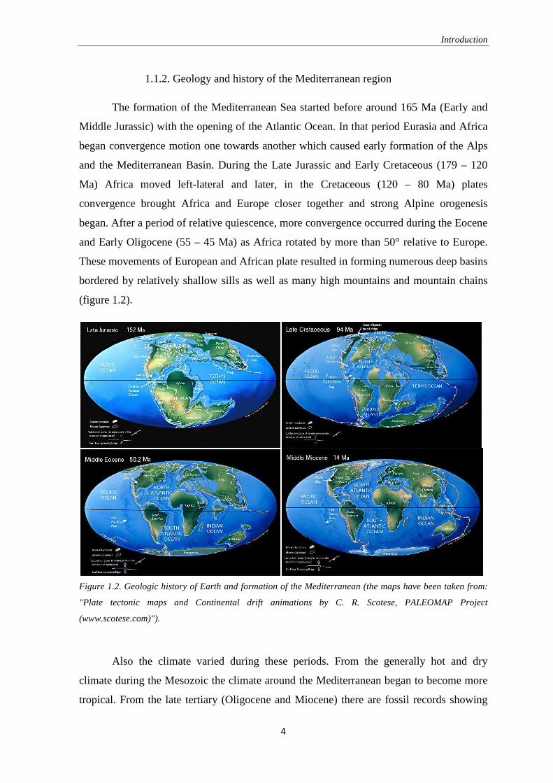
Figure 1.2. Geologic history of Earth and formation of the Mediterranean (the maps have been taken from:
"Plate tectonic maps and Continental drift animations by C. R. Scotese, PALEOMAP Project
(www.scotese.com)").
Also the climate varied during these periods. From the generally hot and dry
climate during the Mesozoic the climate around the Mediterranean began to become more
tropical. From the late tertiary (Oligocene and Miocene) there are fossil records showing
Introduction
5
that the vegetation was evergreen rainforest and laurel forests. By the end of the Miocene
tropical elements disappear from the fossil records indicating the decrease of temperature
and the start of the climate very similar to the present one, during the Pliocene (the
temperature were probably just few degrees higher then today). The cooling continued
through whole Pliocene to arrive to well-known cold period in the Pleistocene (2.5 – 2.1
Ma) after which the present climate started.
There are two events that significantly influenced the wildlife in Mediterranean:
The Messinian salinity crisis is event that begun at 5.96 Ma and started as a result of
uplifting along the African and Iberian plate which resulted in closing of the Mediterranean
Sea. Since evaporation of the Mediterranean Sea is much stronger then the water input
from the rivers and the precipitations it led to lowering of sea level in the whole Basin. The
Mediterranean Sea became a disjunct mosaic of large salty lakes located in the deepest
parts of the Basin. Recently the depth of the evaporates demonstrated that this evaporation
did not occur just once during the long period. The connection of the Mediterranean Sea
and the Atlantic Ocean was closed and reopened probably 8-10 times. The Messinian
salinity crisis, that finally ended 5.33 Ma, was probably the most dramatic event that
occurred during the Cenozoic era. The most parts of the Basin in these dry periods were
deserts and while for the marine organisms this meant termination for some terrestrial
organisms it opened new land-bridges that could offer some new migration opportunities
and mix the previously separated populations (Thompon 2005).
The Pleistocene (1.8 Ma – 15 000 BP) was another dramatic period for the Mediterranean
Basin. Due to the strong cooling of the climate big quantity of the water concentrated in
continental ice sheets 1500 to 3000 meters thick, resulted in temporary sea level drops of
230 m or more over the entire surface of the Earth. This, once again, caused drying out of
some of the parts of the Mediterranean (for example the half of the Adriatic Sea) while the
most of the Mediterranean islands become connected with the mainland, creating once
again the bridges for plants and animals (Blondel & Aronson 1999).
Introduction
6
1.1.3. Pleistocene in the Mediterranean region
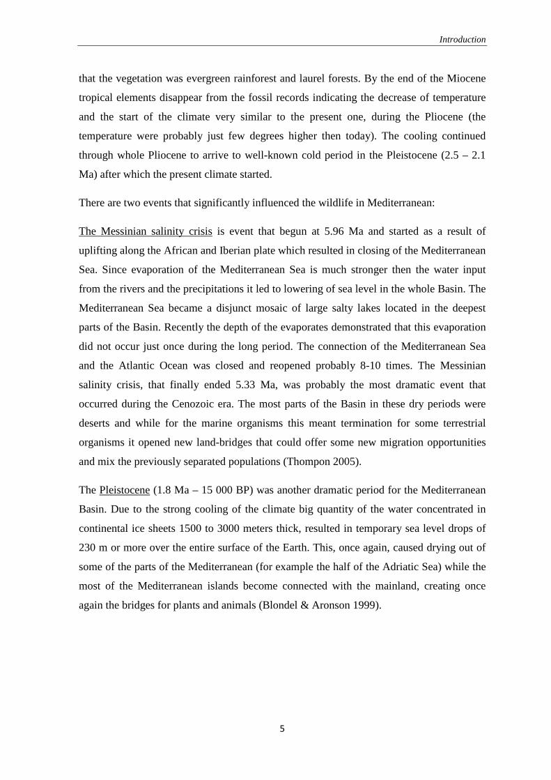
The Pleistocene lasted from about 2 588 000 to 11 700 years ago, spanning the
world's recent period of repeated glaciations. The climate was marked by repeated glacial
cycles where continental glaciers were pushed to the 40th parallel somewhere (figure 1.3).
It is estimated that, at maximum glacial extent, 30% of the Earth's surface was covered by
ice. The mean annual temperature at the edge of the ice was −6°C and at the edge of the
permafrost 0°C (Blondel & Aronson 1999). The effects of glaciation were global.
Antarctica was ice-bound throughout the Pleistocene as well as the preceding Pliocene.
The Andes were covered in the south by the Patagonian ice cap. There were glaciers in
New Zealand and Tasmania. The current decaying glaciers of Mount Kenya, Mount
Kilimanjaro, and the Ruwenzori Range in east and central Africa were larger. Glaciers
existed in the mountains of Ethiopia and to the west in the Atlas Mountains. In the northern
hemisphere, many glaciers fused into one. The Cordilleran ice sheet covered the North
American northwest; the east was covered by the Laurentide. The Fenno-Scandian ice
sheet rested on northern Europe, including Great Britain; the Alpine ice sheet on the Alps.
Figure 1.3. Earth during the last glacial period (the map has been
taken from: "Plate tectonic maps and Continental drift animations
by C. R. Scotese, PALEOMAP Project (www.scotese.com)").
It is not completely known where Mediterranean vegetation persisted during the
glacial periods but the most number of refugia occurred in the southern Iberian and
Apennine Peninsula, Balkans, Middle East and North Africa. Vegetation of the southern
Europe in that period was the vegetation dominated by grasses and Artemisia species.
Introduction
7
Essentially land was covered by the steppe vegetation adapted to the lack of water as well
as low temperature (Thompon 2005). Médail & Diadema (2009) identified 52 refugia
within the Mediterranean region, 33 situated in the western Mediterranean Basin and 19 in
the eastern part. It is hard to know how numerous the long term persistent tree cover was
but it has been clearly demonstrated it existed. Beech forests, for example, during the last
glacial period survived in many regions in Italian and Balkan peninsulas, but much less
data have been found for the Iberian Peninsula (Magri et al. 2006). Interesting is that the
fossil and genetic data show that beech survived the last glacial period in multiple refuge
areas, as in Mediterranean as in the central Europe, but that the Mediterranean refuge areas
did not contribute to the colonization of central and northern Europe (Magri et al. 2006).
Oak species, on the other hand, inhabited Iberian, Italian and Balkan Peninsula (probably
escaping on the mid-altitude in mountainous regions seeking for more precipitations) from
where they dispersed all around the north Europe taking various, often distant, passages
(Petit et al. 2002). Recently it seems to be more and more evident that the vision of the
Europe without forest needs to be reconsidered and the forest probably used to survive also
northernmost then it was thought. Macrofossil (Willis et al. 2000) as well as computer
simulated analyses indicate that nemoral trees were probably largely confined to the
traditional southern refugia, but, with many species being potentially widespread within
this region, while many boreal tree species may have been widespread not only in these
southern areas, but also in Central and Eastern Europe, including the Russian Plain
(Svenning et al. 2008). The fast expansion of the forest in Holocene, when the climate
became warmer, testifies that several refugia existed also between the eastern margin of the
Scandinavian ice sheet and the Ural Mountains (Väliranta et al. 2011).
1.1.4. Evolution after the Pleistocene and human impact on the vegetation
After the last glaciation the warming happened pretty fast and the pioneer plants
spread fast from their refugia to the uninhabited areas. The deciduous forest spread from
the Mediterranean area north at rates of about 102 – 103 m per year. The possible problems
for the first plants were probably the grazers that were often slowing down the forest
evolvement. While northern Europe was being reforested the Mediterranean region was
slowly losing the forest cover as the shrublands started to become frequent. Responsible
for these changes is the climate that became drier and caused frequent forest fires during
Introduction
8
the summer, often combined with strong Mediterranean winds. It is also necessary to
regard the human activity, which, right from the end of the Pleistocene, started to be more
present in the major part of the Basin. There are contrast opinions whether the vegetation
has changed due to the climate changes or due to the human presence but doubtless the
moment when human started to use fire for creating pastures and agricultural field meant
the drastic change for the Mediterranean environment (Thirgood 1981).
No other place on the Earth has such a strong and constant contact of the nature and
human as Mediterranean Basin. Since the region was inhabited by various cultures from
the beginning of the western civilization it is often hard to describe and imagine the
original vegetation of some particular parts of the Mediterranean. While existing forests or
even relict trees may indicate the original woodland in general terms, the cover has been
widely reduced on many sites to one of sparse annuals and unpalatable perennials.
Therefore all the present vegetation must always be interpreted considering the possible
human activities from the past. Less resistant and more valuable species have been reduced
(or concentrated in small limited areas) while the big areas have been covered with
degraded forest types such are maquis (a biome consisting of densely growing evergreen
shrubs) and garrigue (more degraded bush associations with open spaces), or even batha,
presenting the lowest vegetation formation containing scattered low scrubs with annual
plants scattered on the rocky ground. Other point of view does not consider maquis
degraded land formed by the human but is an original type of the vegetation, evolving as a
result of the particular climatic and environmental phenomenon such are extreme droughts
during the summer, periodical freezing winters, extremely hot summers, strong winds and
common natural fire (Thirgood 1981).
A valuable source of information when studying the phytogeography of the
Mediterranean plants are the historical records demonstrating the management practices of
the forests in the antiquity. From an early date, trees were moved from place to place, thus
Darius (530 – 522 B.C.) wrote to his steward, Gadatar: “… you are taking trouble over my
estates, in that you are transferring trees and plants from beyond the Euphrates to Asia
Minor”. In Roman times, the coppice woods with annual coupes were common and were
termed Silvae caeduae. Pliny the Older, in his Historia Naturialis, mentions eight year
rotations for chestnut for the production of vine stakes and eleven years for oak (Thirgood
1981). The writers Vergil, Varro, Columella and Pliny, all included directions on the

Introduction
9
growing of timber trees in their treatises. Pliny also remarks that the mountain slopes
around his villa were “covered with plantations of timber” (Pliny the Younger, 1st century
AD). It is considered that a considerable amount of planting was done by Etruscans,
Greeks, Romans and Arabs, and that especially big number of Pines were moved throw-out
the Mediterranean basin. Pinus pinea L. is perhaps the best known example about which
there are numerous different opinions. As it is an edible plant it was planted widely.
Theories about being the Lebanon-origin tree, being brought to other parts of the
Mediterranean already by Etruscans, contrast the one based on which it was always
distributed from western to eastern Mediterranean (Thirgood 1981).
1.2. Studied species
1.2.1. Genus Pinus
1.2.1.1. Evolution of pines
Gymnosperms are woody seed plants of huge economic and ecological importance.
They are often considered ancient plants, even “living fossils”; since, nevertheless they
developed very early in geologic history (probably in the Middle Devonian, 365 million
years ago), their species abundance nowadays is very low comparing it to the one of the
angiosperms. Recently it has been discovered that angiosperms and gymnosperms
probably developed in the same time but with angiosperms’ diversification happening very
slowly at the beginning (Megallon 2010, Smith et al. 2010). This is why the term “living
fossils” is to be reassessed. Gymnosperms’ low number of species, earlier explained as the
low evolutionary rate but recently demonstrated it is the same or even bigger than in the
angiosperms (Crisp & Cook 2011), should be justified by the big extinctions in the past.
The biggest extinction of gymnosperms occurred relatively recently, in the end of the
Eocene, and was caused by strong global cooling and drying. Number of conifer species
nowadays is reduced to only 850 to 1200 species with more than a third of the species
belonging to the Pinaceae family. More than half of the species under this family are
included in the remarkable genus Pinus (containing more than 100 species).

Introduction
10
The earliest known pine, Pinus belgica, is found in the Early Cretaceous (about 130
million years ago) in Belgium, followed by finding of another 25 pine species from the
same period. These Mesozoic pines were dispersed from 31° – 50° N latitude and were
spreading from east to west of Laurasia, as North America and Europe were still joint. At
this latitude the climate was stable during the year with temperature 10° – 20°C higher than
today and with moderate rainfalls. Next geologic period, Paleogene, was characterized by
strong climatic changes having a big impact on pine populations. As a result of a strong
temperature increase, tropical forest spread throughout the middle latitudes overcoming the
previously growing pines (for which the temperature as well as moisture became too high).
From this period the pine pollen was present only on extremely high or low latitudes and
several scarce refugia. Global cooling at the end of Eocene, allowed the dispersion of the
pines once again so, contrary to the most of the gymnosperms, pine families marked a big
increase. This period is considered to be the period with the biggest impact on the pine
genetic biodiversity (Millar 1993). By the end of Eocene most of the pine subsection were
developed and were dispersed generally on the same places as today (Millar 1998).
Pleistocene glaciations do not seem to have affected the pine populations so strongly. In
central and southern Europe pine population probably survived without significant losses,
while from the northern Europe they were refuging and re-spreading in each interglacial.
For example, there are evidence that Scots Pine (Pinus sylvestris L.) lived on 30 locations
in Carpathian plane in the periods from 32 000 – 25 000, 23 000 – 20 000 and 18 000 – 16
000 years BP (Rudner & Sümegi 2001), demonstrating the high resistance of the pines on
then-current conditions. Increase of the pine populations in southern and central Europe
started already between 15 000 and 12 000 years ago, and arrived to the northernmost of
the continent about 5 700 years ago (when pines dominated even in Finland). It is
interesting to point out that the pine coverage at that period was bigger than nowadays,
especially in North Europe. From yet not explainable reasons (regional climate changes,
volcanic eruptions, anthropogenic pressures or change in fire frequency are the most
acceptable theories) between 4 800 and 4 400 years BP another big decrease of the pine
pollen occurred and brought pine populations down to present dimensions (Willis et al.
1998).

Introduction
11
1.2.1.2. Pines of the Mediterranean Basin
Mediterranean pines according to Klaus (1989), represent an extremely
heterogeneous assembly and consist mainly of relic pines from the Cretaceous–Tertiary
period. Based on the pollen findings they were present in the Basin about 3,5 million years
ago. In fact they were probably periodically present much earlier but they started to evolve
and to inhabit wide territory at the period when the climate of the area started to become
dryer (end of Miocene, 5 million years ago) since the resistance to drought conditions is
the biggest advantage of the pines in the Mediterranean area. Nowadays there are ten pine
species inhabiting the Mediterranean Basin and they play an important role in
Mediterranean habitats. There have been many discussions whether Mediterranean pines
could form the climax vegetation, therefore present the stabile population or not. Generally
pines in Mediterranean form a pioneer vegetation or intermediate step forward to the more
stable vegetation but it is also possible to find the pine-dominated climax communities,
especially the ones irreversibly modified by human activity. In any case distribution of the
pine populations in Mediterranean is closely related to the human activities for over 10 000
years and it is impossible to discuss pine vegetation in Mediterranean without considering
forest fire and cutting caused by man as well as reforestation processes (Barbéro et al.
1998).
1.2.1.3. Genetic diversity of pines
Pines are often considered taxonomically complicated genus due to their big
capacity of the interspecific hybridization (Bucci et al. 1998). There are, also, many
closely related taxa with small, but notable morphologic differences, whose taxonomical
status have been doubtable and have been changing often through the time. This itself
demonstrates the big diversity that can be found inside the genus. Pines are extremely
genetically diverse organisms due to the lack of complete barriers to hybridization, high
fecundity and high dispersal of the pollen and seeds (Ledig 1998). The huge production of
pollen as well as pollen grains with two “wings”, air bladders between the intine and exine
of the pollen grain, are its special adaptations for anemophily and allows them to spread
and exchange their genetic material widely. To assure long distance dispersal, seed of
almost all the pines have a wing which facilitates their wind transportation.

Introduction
12
Apart the interspecific hybridization ability, another characteristic causing the
difficulties in the beginning of the genetic analyses is the inheritance of organellar DNA in
pines, which is different from the one in the angiosperms. In pine species mtDNA is being
inherited maternally as in all the angiosperms, while the cpDNA is being inherited
parentally (Neale & Sederoff 1989).
The biggest specification of the genus Pinus, as mentioned before, occurred in
Eocene. As a result of the climatic changes in that period nowadays there are more and less
polymorphic pine species. Some of the species inhabited various refugia and in that period
managed to differentiate one from each other while other species, located in smaller
populations in which they often suffered from the bottle neck effect, nowadays have
extremely low diversity rate. One of such examples is widely distributed red pine, Pinus
resinosa Ait., which passed through genetic bottle neck during the last glacial period and
therefore nowadays is one of the most genetically depauperate conifer species in North
America. After numerous temptations with different genetic methods with no results
finally 5 polymorphic nuclear microsatellites managed to distinguish “northeastern” from
the main population (Boys et al. 2005). European Black Pine, on the other hand,
demonstrated big genetic diversity using many different methods and its vast
polymorphism will be discussed in details below.
1.2.1.4. Systematics of genus Pinus
Systematics of the genus Pinus has been a complicated issue for a long period with
huge number of articles published about this theme (Gernandt et al. 2005, Kaundun &
Lebreton 2010). Recent classification based on chloroplast DNA analyses confirms the
existence of two subgenus; Pinus (Diploxylon or hard pines) and Strobus (Haploxylon or
soft pines). In the first group there are two sections (Pinus and Trifoliae) and five
subsections and in the second one, two sections (Parrya and Quinquefogliae) divided in six
subsections (Gernandt et al. 2005). Based on morphometric and biochemical (flavonoids)
parameters it has been discovered that the subgenus Strobus (Holarctic group with 5
needles) is the ancestral one, while in the subgenus Pinus (Lauroasian group with two or
three needles) the most ancient group is Trifoliae. On the other hand the Mediterranean
pines (subsections Pinus and Pinaster from the section Pinus) are the most recent ones,

Introduction
13
especially the ones from the subsection Pinaster, growing in the dry and hot climate, which
are highly evolved compared to those from the cold and wet regions (Eurasia and North
America) (Kaundun & Lebreton 2010).
The section Pinus is a huge group containing 3/5 of the pine species, mainly
distributed on south. The subsections are Pinus and Pinaster. Subsection Pinus contains
the species originating from the Eurasia, Mediterranean, Eastern North America and Cuba
and are following species: P. densata Mast., P. densiflora Siebold & Zucc., P.
hwangshanensis W. Y. Hsia, P. kesiya Royle ex Gordon, P. luchuensis Mayr., L.
massoniana Lamb., P. merkusii Jungh. & de Vriese, P. mugo Turra, P. nigra J.F.Arnold, P.
resinosa Sol. ex Aiton, P. sylvestris L., P. tabuliformis Carr., P. taiwanensis Hayata., P.
thunbergii Parl., P. tropicalis Morelet, P. unicata Raymond ex A. DC. and P. yunnanensis
Franch.. Subsecion Pinaster contains the species originating from the Canary Islands,
Mediterranean and Himalayas and they are: P. brutia Ten., P. canariensis C. Sm., P.
halepensis Mill. , P. heldreichii H.Christ, P. pinaster Aiton., P. pinea L. and P. roxburghii
Sarg. (Gernandt et al. 2005).
1.2.1.5. Aleppo pine (Pinus halepensis Miller)
Aleppo pine is a small to medium-size tree, 10-20 m tall. The bark of the young
trees is smooth and light grey; while later it becomes orange-brown, thick and deeply
fissured at the base of the trunk, and thin and flaky in the upper crown. The leaves
("needles") are very slender, 6–10 cm long, distinctly yellowish green and produced in
pairs; usually they fall down after two years. The cones are narrow conic, 5–12 cm long
and 2–3 cm broad at the base when closed, green at first, ripening glossy red-brown when
24 months old. Usually cones grow in the groups of 2-3, they are petiolate on the stem of
up to 2 cm and usually turned down. They open slowly over the next few years, a process
quickened if they are exposed to heat such as in forest fires. The cones open 5–8 cm wide
to allow the seeds to disperse. The seeds are 5–6 mm long, with a 20 mm wing, and are
wind-dispersed (Vidaković 1982).
Aleppo pine is mainly pioneer species adapted to grow in poorer soils with the
ability to grow even on “terra rossa”, clay soil produced by the weathering of limestone, or
on the soils rich of magnesium or iron. It withstands well the climate with periodically
Introduction
14
droughts occurring every year for at least three months and with annual precipitations of
400-300 mm. It is also the common in degraded plant communities. The most stabile
populations are formed in the low maquis biome growing together with Mastic (Pistacia
lentiscus L.), Myrtus (myrtle) (Myrtus communis L.), Phillyrea (Phillyrea sp.) and
Rosemary (Rosmarinus officinalis L.) or in the garrigue plant community with Thymus
capitatus L. and accompanying species. Aleppo pine is one of the most flammable and
fire-prone species in the Mediterranean Basin with the historical notes in which one third
of the population burned (Bernetti 1995). Its strong adaptation to fire is also visible on their
cones that sometimes open several years after the maturation ensuring that, after the fire
(high temperatures make the cones of several generations open at the same moment), big
quantity of the seeds are momentarily ready to sprout (Bernetti 1995).
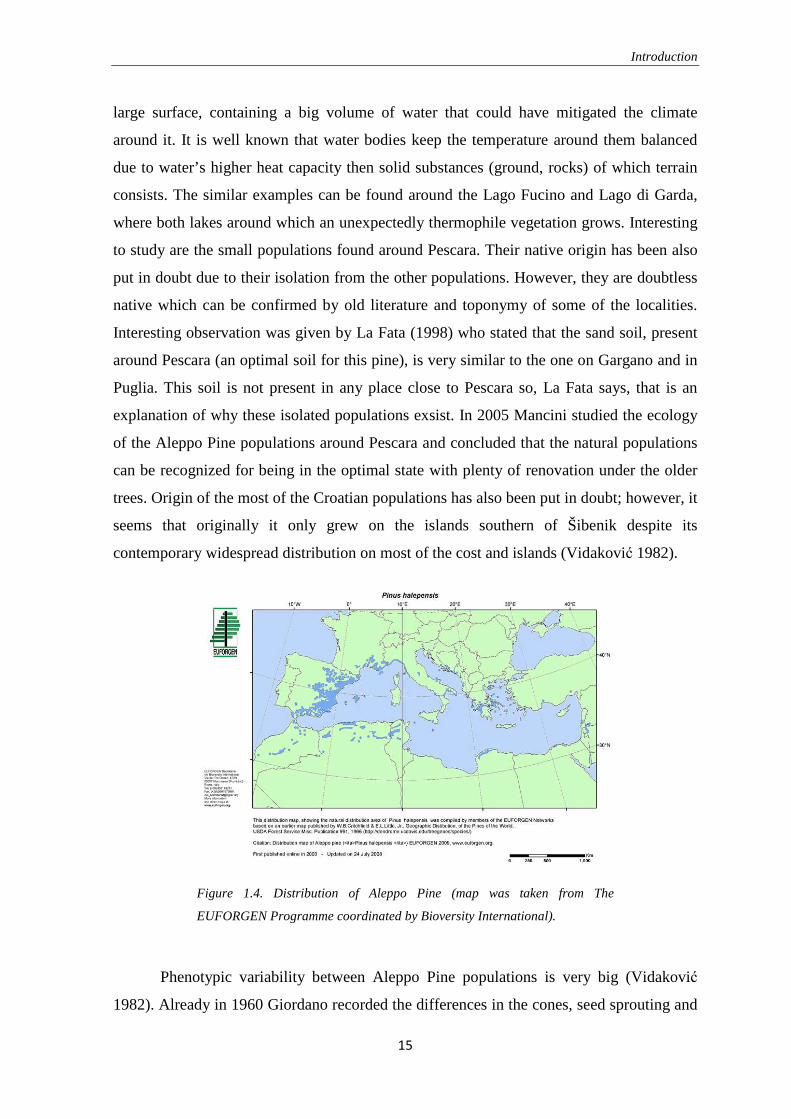
This pine is a strictly Mediterranean species dispersed in Morocco, Algeria, Tunisia
and Libya in Africa, Spain, France, Italy, Croatia, Montenegro, Albania and Greece in
Europe and Turkey, Israel and Jordan in Asia (figure 1.4). It grows from the sea level to
the altitudes of 1500 m (in Morocco and Algeria). As a pioneer species it has been widely
used in reforestation either as a plant to stop soil degradation or to prepare the conditions
for planting broadleaf vegetation. However this pioneer species often got naturalised very
easily so now it is hard to estimate its original distribution. In Italy the biggest spontaneous
or sub-spontaneous populations are found in Apulia (especially on the Gargano Peninsula
and in the provenience of Taranto) (Giordano et al. 1984, Agostini 1969) as well as in
Sardinia and Sicily. The doubtful populations are the ones in Umbria in Valle Spoletina
and in Valle Nerina which are very well naturalised but based on their unusual location and
floristic composition as well as morphological similarity to an Israeli population Schiller &
Brunori (1992) conclude it is a result of an ancient reforestation. Still there is another point
of view stating that the vegetation around the Pine individuals consists of the
Mediterranean flora plants (Strawberry tree, Phylirea, Judas tree, etc.). So, even though it
seems that the location is not natural for the Aleppo Pine since it is located in the
mountainous area, far away from the sea, presence of the other Mediterranean plants heads
to idea that the conditions are not so unsatisfactory after all. Explanation of how certain
Mediterranean plants can be found on the mountains so far away from the sea in the place
nowadays considerably cold place could be found in an ancient Lake Velino that existed
before the Roman period. This lake, before the Romans started drying it out, covered a
Introduction
15
large surface, containing a big volume of water that could have mitigated the climate
around it. It is well known that water bodies keep the temperature around them balanced
due to water’s higher heat capacity then solid substances (ground, rocks) of which terrain
consists. The similar examples can be found around the Lago Fucino and Lago di Garda,
where both lakes around which an unexpectedly thermophile vegetation grows. Interesting
to study are the small populations found around Pescara. Their native origin has been also
put in doubt due to their isolation from the other populations. However, they are doubtless
native which can be confirmed by old literature and toponymy of some of the localities.
Interesting observation was given by La Fata (1998) who stated that the sand soil, present
around Pescara (an optimal soil for this pine), is very similar to the one on Gargano and in
Puglia. This soil is not present in any place close to Pescara so, La Fata says, that is an
explanation of why these isolated populations exsist. In 2005 Mancini studied the ecology
of the Aleppo Pine populations around Pescara and concluded that the natural populations
can be recognized for being in the optimal state with plenty of renovation under the older
trees. Origin of the most of the Croatian populations has also been put in doubt; however, it
seems that originally it only grew on the islands southern of Šibenik despite its
contemporary widespread distribution on most of the cost and islands (Vidaković 1982).
Figure 1.4. Distribution of Aleppo Pine (map was taken from The
EUFORGEN Programme coordinated by Bioversity International).
Phenotypic variability between Aleppo Pine populations is very big (Vidaković
1982). Already in 1960 Giordano recorded the differences in the cones, seed sprouting and
Introduction
16
the growing period between the individuals of the different proveniences and Karschon
(1961) found the morphological differences of the populations growing on different
altitudes in Israel. Turning to the molecular-level analyses the variability was not so
strongly demonstrated. Performing the allozyme analysis in Jordan and Israeli the
variability within populations was high but the one among the populations was not (Korol
et al. 1995). Analysis of resin monoterpenes also showed the small variability between
numerous provenances (Greece, Spain, Morocco, Algeria, Tunisia and Israel), managing to
distinguish only three distinct groups; the Greek, the West European and the North African
one (Schiller & Grunwald 1987). The small genetic within-population diversity was also
recorded with chloroplast microsatellite analyses, probably signalling the strong bottleneck
event that occurred in the past (Morgante et al. 1997). Using the same method Grivet
(2009) explained that the small diversity in the eastern populations shows their initial
origin. From east the colonisation moved towards west, passing over Italy. Italian
peninsula nowadays hosts the most variable population, whose polymorphism is recent and
the result of a strong bottleneck occurred around 18 000 years ago (Grivet 2009).
Turkish Pine (Pinus brutia Tenore)
Turkish Pine is an interesting species, evolutionary very close to Aleppo Pine. It
was considered as a subspecies of Aleppo Pine (P. halepensis subsp. brutia (Ten.) Henry)
(Fukarek 1959) but later they got separated in two distinct species (P. brutia T. and P.
halepensis Mill.) (Gaussen et al. 1964, Pignatti1 1982). Evidence of their close relations
lays in their hybridization capability. Turkish and Aleppo pine hybridization in nature has
been described in Greece (Panetsos 1975) and Turkey (Schiller & Mendel 1995) and on the
plantations in Croatia (Vidaković 1982), Italy (Gola 1924) and France (Vidaković 1982).
More recently this hybridization has been demonstrated with allozymes (Korol et al. 1995)
and chloroplast paternally inherited simple-sequence repeat (cpSSR) markers (Bucci et al.
1998), who showed the direct evidence for hybridization between sympatric populations.
According to allozyme analyses extant Turkish Pine is similar to the progenitors of the
Aleppo Pine (Conkle et al. 1988).
It is distinguishable from the Aleppo Pine for its longer needles, strongly reddish
bark and for the sessile cones grouped two or three together in their particular way. Turkish
Introduction
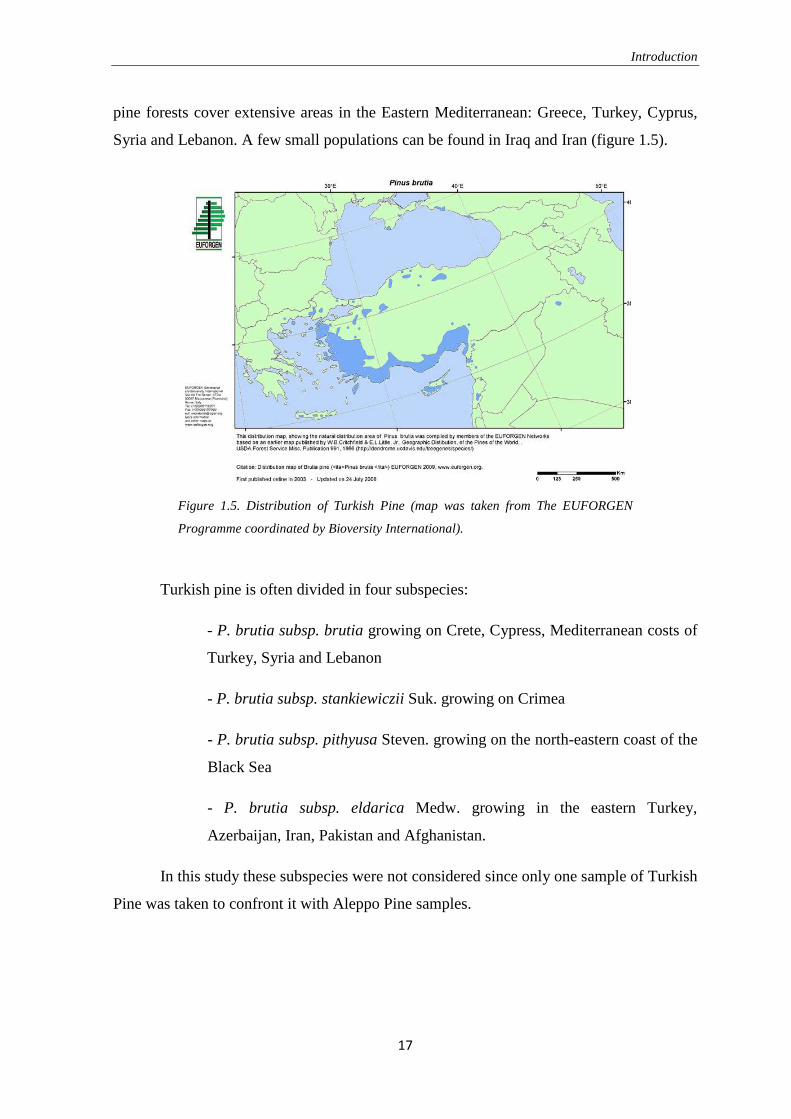
17
pine forests cover extensive areas in the Eastern Mediterranean: Greece, Turkey, Cyprus,
Syria and Lebanon. A few small populations can be found in Iraq and Iran (figure 1.5).
Figure 1.5. Distribution of Turkish Pine (map was taken from The EUFORGEN
Programme coordinated by Bioversity International).
Turkish pine is often divided in four subspecies:
- P. brutia subsp. brutia growing on Crete, Cypress, Mediterranean costs of
Turkey, Syria and Lebanon
- P. brutia subsp. stankiewiczii Suk. growing on Crimea
- P. brutia subsp. pithyusa Steven. growing on the north-eastern coast of the
Black Sea
- P. brutia subsp. eldarica Medw. growing in the eastern Turkey,
Azerbaijan, Iran, Pakistan and Afghanistan.
In this study these subspecies were not considered since only one sample of Turkish
Pine was taken to confront it with Aleppo Pine samples.

Introduction
18
1.2.1.6. European black pine (Pinus nigra Arnold)
European Black Pine is a large coniferous evergreen tree, growing up to 20–55
meters tall and usually straight at maturity. The crown is broadly conical on young trees,
umbrella-shaped on older trees, especially in shallow soil on rocky terrain. The bark is grey
and widely split by black flaking fissures into scaly plates, becoming increasingly fissured
with age. The dark-green leaves ("needles") are growing two together, straight or curved,
rather stiff, 8-16 cm long and 1-2 mm wide. Black pine is a monoecious wind-pollinated
conifer and its seeds are wind dispersed. Flowering occurs every year, although seed yield
is abundant only every 2–4 years. Ovulate and pollen cones appear from May to June,
depending on the local climate. Fecundation occurs 13 months after pollination. The
mature seed cones are 5–10 cm long and 2-4 cm wide, sessile and horizontally spreading
with rounded scales. They ripen from September to October of the second year, and open
in the third year after pollination. Cones contain 30–40 seeds, of which half can germinate.
The seeds are dark grey, 6–8 mm long, with a yellow-buff wing 20–25 mm long; they are
wind-dispersed when the cones open from December to April (Isajev et al. 2003,
Vidaković 1982). These are general morphological characteristics but it is important to
note that between the populations there is a great diversity in morphology as well as in
ecology.
European Black Pine is moderately fast growing, at about 30–70 centimetres per
year. The tree can be long lived, with some trees over 500 years old. It needs full sun to
grow well (is intolerant of shade) and is resistant to snow and ice damage. The optimal
altitudinal range of Black Pine is between 800 to 1500 m a.s.l., but this also varies between
subspecies (for example P. nigra subsp. dalmatica which grows on the Adriatic islands).
Diverse pine populations grow on various soil types under various external conditions, for
example P. nigra in Sicily and Calabria grows on the silicate soils in very dry habitat, P.
nigra in Valletta Barrea (Abruzzi) and P. nigra subsp. dalmatica (Adriatic coast) on the
calcareous soils and also extremely dry habitat while the P. nigra in Friuli grows on the
calcareous soils but with the annual humidity double from the former ones (Gellini &
Grossoni 1996). Regarding the ecology of the species Black Pine is a species growing on
the sub Atlantic mountainous stripe; on the superior margin of heliophilic broadleaf
vegetation and inferior of the Mediterranean forests of Pubescent Oak (Quercus pubescens
Willd.) with the medium temperatures from 7 to 12°C and with a medium of the coldest

Introduction
19
month over -2°C. However even here there are differences between the populations. Black
Pine from the Alps (P.nigra subsp. nigra) is less thermophylic and more resistant on the
low temperatures while the Pine from Calabria (P. nigra subsp. laricio) seems to suffer
more from the low temperatures when planted out of his range (Bernetti 1995).
Another particularity of the European Black Pine is its discontinuous distribution.
Naturally it inhabits southern Europe, north-western Africa and Asia Minor. In southern
Europe distribution covers the central and eastern Iberian Peninsula, southern France, Alps
and Apennines, arriving till the very southern part of the Italian Peninsula as well as on
Corsica and Sicily. From the Alps it follows the line of the Dinaric Alps, spreading on
southern Adriatic islands. From Bulgaria and Greece it spreads to Asia Minor, and over
Romany it spreads to Crimea and Caucasus (Vidaković 1982). Due to its disjunct
distribution under P. nigra group there have been recorded significant morphological
differences that brought to discrimination of the numerous subspecies whose status and
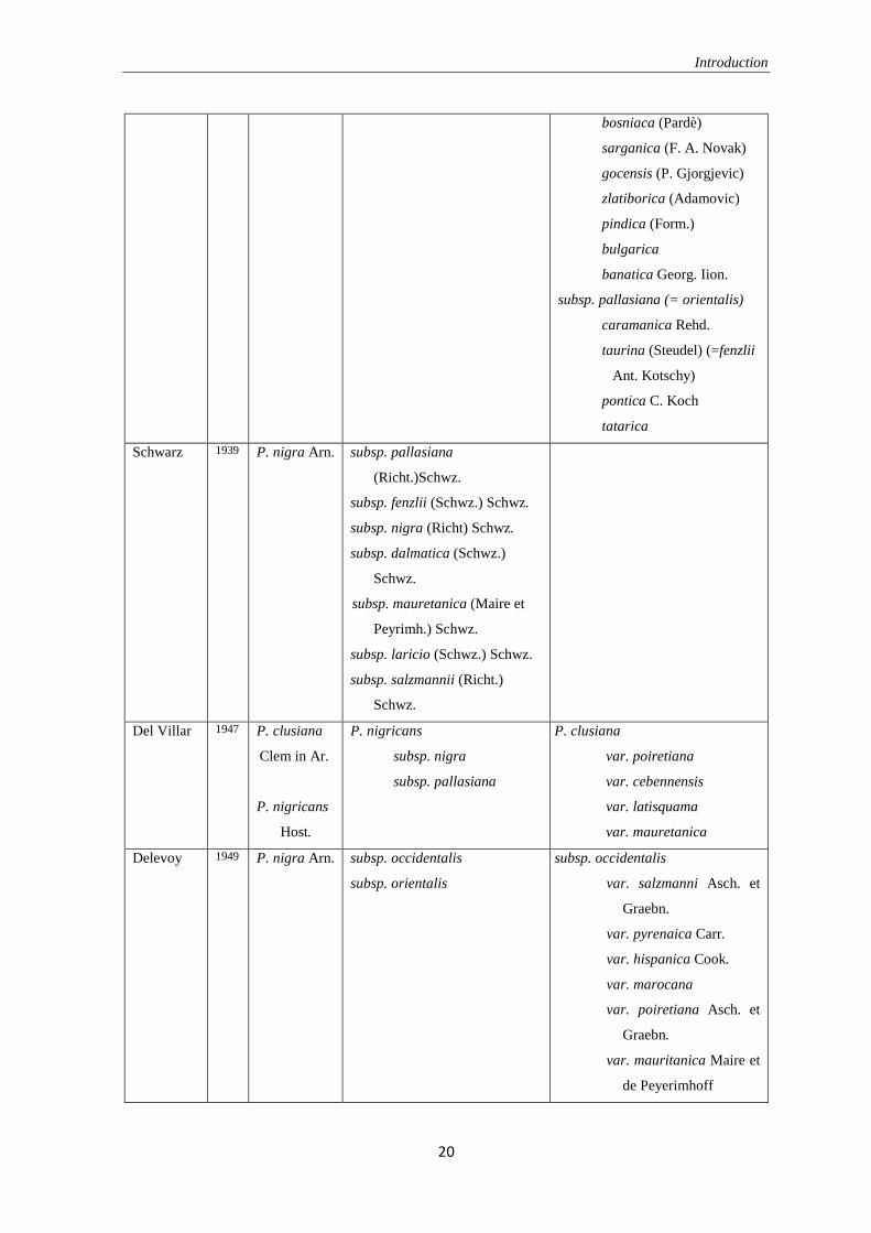
acceptance by the botanists have been changing during the time. Table 1.1 shows the most
of the classification made by numerous researchers.
Author Year Species Subspecies Varieties
Longo-
Ronniger
1903
-
1924
P. nigra Arn. subsp. laricio Poir. (Spain,
France, Corsica, Calabria, Etna)
subsp. nigra Arn. (Austria,
Balkan, Greece, Crimea,
Turkey, Cyprus)
Svoboda 1935 P. nigra Arn. subsp. salzmanni (Dunal-Asch-
Gräb.)
subsp. poiretiana (Asch-Gräb.)
subsp. nigricans Host.
subsp. pallasiana (Lamb.)
Holmboe (= orientalis
Kotschy)
subsp. salzmanni
mauretanica (Maire
Peyerynhof)
hispanica Ronninger
(Cook)
pyrenaica (Gran-Godr.)
cevennensis Rehd.
subsp. poiretiana
corsicana (Laud.)
calabrica (Schneid.)
barrea
subsp. nigricans
austriaca Höss
dalmatica Vis.
Introduction
20
bosniaca (Pardè)
sarganica (F. A. Novak)
gocensis (P. Gjorgjevic)
zlatiborica (Adamovic)
pindica (Form.)
bulgarica
banatica Georg. Iion.
subsp. pallasiana (= orientalis)
caramanica Rehd.
taurina (Steudel) (=fenzlii
Ant. Kotschy)
pontica C. Koch
tatarica
Schwarz 1939 P. nigra Arn. subsp. pallasiana
(Richt.)Schwz.
subsp. fenzlii (Schwz.) Schwz.
subsp. nigra (Richt) Schwz.
subsp. dalmatica (Schwz.)
Schwz.
subsp. mauretanica (Maire et
Peyrimh.) Schwz.
subsp. laricio (Schwz.) Schwz.
subsp. salzmannii (Richt.)
Schwz.
Del Villar 1947 P. clusiana
Clem in Ar.
P. nigricans
Host.
P. nigricans
subsp. nigra
subsp. pallasiana
P. clusiana
var. poiretiana
var. cebennensis
var. latisquama
var. mauretanica
Delevoy 1949 P. nigra Arn. subsp. occidentalis
subsp. orientalis
subsp. occidentalis
var. salzmanni Asch. et
Graebn.
var. pyrenaica Carr.
var. hispanica Cook.
var. marocana
var. poiretiana Asch. et
Graebn.
var. mauritanica Maire et
de Peyerimhoff

Introduction
21
subsp. orientalis
var. calabrica Schneid.
var. austriaca Asch. Et
Graebn.
var. hornotica Beck
var. gočensis Đorđ.
var. dalmatica Vis.
var. bosniaca Elwes
var. banatica Georgescu
var. pallasiana Asch. et
Graebn.
var. caramanica Hort.
var. fenzlii Ant. et
Kotsch.
Vidaković 1957 P. nigra Arn. subsp. austriaca Höss
subsp. gočensis (Đorđ)
subsp. dalmatica (Vis.) Schwrz.
subsp. pallasiana (Lamb.)
Holmonn
subsp. calabrica (Scheid.)
subsp. corsicana (Loud.) Fuk.
subsp. salzmanni (Dunal)
Franco.
subsp. gočensis
var. illyrica
Fukarek 1958 P. clusiana
(Clemente in
Arias)
P. laricio
(Poiret in
Lamk)
P. nigricans
Host.
P. pallasiana
Lambert.
P. clusiana:
P. mauretanica (Maire-
Peyerynhof)
P. salzmannii (Maire et
Peyerinhof)
P. hispanica (Cook)
P. laricio
P. corsicana (Loud)
P. calabrica (Delamare)
P. nigricans
P. austriaca (Höss)
Novak
P. illyrica (Vidakovic)
P. dalmatica (Visiani)
P. pindica (Formanek)
P. italica (Hosschstett.)
P. salzmannii
var. pyrenaica (Gren et
Godr)
P. illyrica
var. gocensis (Dord)
P. caramaniva
var. zhukovskiana (Palibin)
var. senneriana (Saatz.)

Introduction
22
P. pallasiana
P. banatica (Georg. Et
Ion.)
P. tatarica
P. caramaniva (Loud)
P. fenzlii (Ant. Et
Kotschy)
Gaussen et
al.
1964 P.nigra Arn. P. nigra subsp. pallasiana
P. nigra subsp. dalmatica
P. nigra subsp. salzmannii
P. nigra subsp. laricio
P. nigra subsp. nigra
Röhrig 1966 P. nigra Arn. var. pyrenaica (La Peyrouse)
Goron
var. salzmanii (Dunal) Asch. and
Graebner
var. poiretiana (Ant.) Schneider
var. calabrica (Loud.) Schneider
var. nigra (Hoess) Asch. and
Graebner
Debazak 1977 P. nigra Arn. P. n. subsp. clusiana (Clemente
in Arias)
P. n. subsp. laricio (Poiret in
Lamk)
P. n. subsp. nigricans Host.
P. n. subsp. pallasiana Lambert.
var. mauretanica (Maire-
Peyerynhof)
var. salzmannii (Maire et
Peyerinhof)
var. hispanica (Cook)
var. corsicana (Loud)
var. calabrica (Delamare)
var. austriaca (Höss) Novak
var. illyrica (Vidakovic)
var. dalmatica (Visiani)
var. pindica (Formanek)
var. italica (Hosschstett.)
var. banatica (Georg. Et Ion.)
var. tatarica
var. caramaniva (Loud)
var. fenzlii (Ant. Et Kotschy)
Table 1.1. The classification made by various researchers in past.
Introduction
23
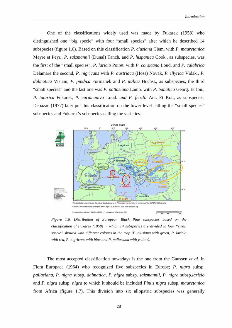
One of the classifications widely used was made by Fukarek (1958) who
distinguished one “big specie” with four “small species” after which he described 14
subspecies (figure 1.6). Based on this classification P. clusiana Clem. with P. mauretanica
Mayre et Peyr., P. salzmannii (Dunal) Tanch. and P. hispanica Cook., as subspecies, was
the first of the “small species”, P. laricio Poiret. with P. corsicana Loud. and P. calabrica
Delamare the second, P. nigricans with P. austriaca (Höss) Novak, P. illyrica Vidak., P.
dalmatica Visiani, P. pindica Formanek and P. italica Hochst., as subspecies, the third
“small species” and the last one was P. pallasiana Lamb. with P. banatica Georg. Et Ion.,
P. tatarica Fukarek, P. caramaniva Loud. and P. fenzlii Ant. Et Kot., as subspecies.
Debazac (1977) later put this classification on the lower level calling the “small species”
subspecies and Fukarek’s subspecies calling the varieties.
Figure 1.6. Distribution of European Black Pine subspecies based on the
classification of Fukarek (1958) in which 14 subspecies are divided in four “small
specie” showed with different colours in the map (P. clusiana with green, P. laricio
with red, P. nigricans with blue and P. pallasiana with yellow).
The most accepted classification nowadays is the one from the Gaussen et al. in
Flora Europaea (1964) who recognized five subspecies in Europe; P. nigra subsp.
pallasiana, P. nigra subsp. dalmatica, P. nigra subsp. salzmannii, P. nigra subsp.laricio
and P. nigra subsp. nigra to which it should be included Pinus nigra subsp. mauretanica
from Africa (figure 1.7). This division into six allopatric subspecies was generally

Introduction
24
followed in all the studies recently performed, regarding morphology, anatomy and
phytogeography (Barbéro et al. 1998). Breeding experiments have shown that all
geographic subdivisions of P. nigra were mutually crossable and gene flow was very
efficient (Vidaković 1991).
Pinus nigra subsp. mauretanica (Maire et Peyerimh.) Heywood covers only a few
hectares in the Rif Mountains of Morocco and the Djurdjura mountains of Algeria. Pinus
nigra subsp. salzmannii (Dunal) Franco (syn: P. n. clusiana, P. n. pyrenaica) covers
extensive areas in Spain (over 350 000 ha from Andalucia to Catalunia and on the southern
slopes of the Pyrenees) and is found in a few isolated populations in the Pyrenees and
Cévennes in France. It is sometimes referred to as the Pyrenean pine. These three groups
were previously united in Pinus clusiana Clem. containing P. mauretanica, P. salzmanni
and P. hispanica (Fukarek 1958). Pinus nigra subsp. laricio (Poiret) is found in Corsica
(Corsican pine) spreading over 22 000 ha, in Calabria (where it is also recognized as P. n.
l. calabrica, the Calabrian pine) and in Sicily. Pinus nigra subsp. nigra (syn: P.n. austriaca
Höss, P.n. nigricans Host, the Austrian pine) is found from Italy in the Apennines to
northern Greece through the Julian Alps and the Balkan mountains, covering more than
800 000 ha. Pinus nigra subsp. dalmatica (Vis.) Franco, the Dalmatian pine, is found on a
few islands off the coast of Croatia and on the southern slopes of the Dinaric Alps. Pinus
nigra subsp. pallasiana (Lamb.) Holmboe covers extensive areas, mostly in Greece and
Turkey (2.5 million ha, 8% of total forest area) and possibly as far west as Bulgaria. It can
also be found in Cyprus and the Crimea. It is sometimes referred to as the Crimean pine.

Introduction
25
Figure 1.7. Distribution of European Black Pine subspecies based on the classification
of Gaussen et al. in Flora Europaea (1964).
On the molecular level fewer analyses have been made. Nikolić & Tucić (1983)
examined isoenzyme patterns of esterase, acid phosphatase and leucine aminopeptidase in
dormant seeds on the samples from the 13 former Yugoslavian and several Mediterranean
populations and, even though they did not find the expected pattern of differentiation,
marked a notable inter-population diversity. Raffi et al. (1996) detected 39 different foliar
terpenoids in 41 various Mediterranean populations and suggested three groups in western
Europe: an eastern Pyrenean and continental France group (subsp. salzmanii); Corsican
group showing affinities with Sicily and southern Apennines (subsp. laricio); and the
eastern group comprising Alps and Balkan (subsp. nigra and dalmatica). Another terpene
study made by Gerber et al. (1995) followed the classification of Röhrig (1966) with
following varieties: pyrenaica from Spanish populations, salzmanii from France,
poiretiana from Corsica, calabrica from Calabria and nigra from the Alps, central
Apenines and Balkans; but with an authors’ note that further genetic analyses should be
made on the Eastern populations. Liber et al. (1999) detected genetic diversity in Croatian
populations of Black pine using the method of random amplified polymorphic DNA
(RAPD), but failed in finding differences analysing restriction fragment length

Introduction
26
polymorphisms (RFLP) of the evolutionary conservative chloroplast DNA. Using the same
method (RAPD) big genetic diversity has been found also between the populations of P.
nigra subsp. nigra in Serbia (Lucić et al. 2010). Finally, Afzal-Rafii and Dodd (2007) used
chloroplast simple sequence repeat (cpSSR) to study the west Mediterranean populations
and found strong barriers separating Alps from Calabria and Corsica, southern Spain from
the Pyrenees and Corsica from Sicily and Calabria. They recorded very high diversity
between the populations and concluded that it is among the highest reported for pines,
close to the level for species differentiation between P. eldraica and P. brutia (Bucci et al.
1998). The authors also come to the conclusion that the existing populations persisted in
situ at least during the last full glacial stage therefore are not the result of the recent
decolonisation. SSR methodology (in this case both cpSSR and nuSSR markers) was also
used to estimate the genetic differences and relationships between the populations from
Sila, Aspromonte, Etna and Corsica (P. nigra subsp. laricio populations) but the relatively
weak differentiation level was observed so the conclusion of the study was that the high
level of seed and pollen flow was the probable cause of the low diversity and mixed
populations (Bonavita 2012).
Between the mentioned subspecies it is often possible to find the intermediate
entities. These intermediate populations could be a sign of an ancient hybridisation. One
such a zone could have been the Apennines where many authors expressed their doubts
and theories. Apparently populations in the central Italy morphologically seem to be a
mixture between the P. nigra subsp. nigra and P. nigra subsp. laricio. The first population
of the Apennines studied was the one of Villetta Barrea in Abruzzo. The first author
recording the Black Pine of Villetta Barrea as a particular entity is Nageli already in 1929
when he noted that it was a native population of Black Pine in Abruzzi. The authors later
considered this pine as a P. nigra subsp. nigra (often specifying it to be var. italica) are
Novák (1953), Röhrig (1957) and De Phillippis (1958); while many more note its
similarity also to the Calabrian Pine samples (P. nigra subsp. laricio) and therefore often
record the Pine of Villetta Barrea as an intermediate species between the P. nigra subsp.
nigra and P. nigra subsp. laricio (Pavari 1931, Fukarek 1958, Morandini 1966, Gellini
1968 and Paci et al. 1988). Another interesting population of Pinus nigra in Abruzzi is the
one on the Majella Mountain. Undoubtedly native population can be found in the Cima
della Stretta over Fara San Martino (Chieti) where the trees are about 500 years old in the
Introduction
27
overhanging walls impossible for the human access and reforestation. This population was
less known than the ones in Villetta Barrea until Schwarz (1939) based on various
anatomic characteristics declared to see no differences from the Black Pine from Calabria,
therefore puts it in the laricio subspecies. Tammaro and Ferri (1982) wrote a description of
the population of Fara San Martino after which, even though the description is more
similar to the Corsican Pine (Bruschi et al. 2005), they conclude it is probably one of the
populations of P. nigra subsp. italica (the term taken from the classification of Fukarek
(1958) which now should be called P. nigra subsp. nigra var. italica). Bruschi et al. (2005)
preformed the detailed anatomical and genetic analyses comparing the samples from Fara
San Martino and Villetta Barrea and came to the conclusion that there is no notable
difference from one to another and that both of them should be affiliated to the P. nigra
subsp. italica group.
1.2.2. Genus Celtis
Celtis, commonly known as hackberries, is a genus of about 70 species. Previously
it was included either in the elm family (Ulmaceae) or a separate family, Celtidaceae, but
chloroplast DNA analyses put it in an expanded hemp family (Cannabaceae) (Wiegrefe
1998). The first fossil records of the genus come from the Oligocene and cover the large
territory from France, Germany, Czech Republic, Poland, Hungary, Austria, Bulgaria and
Moldavia to Kazakhstan. These fossils belong to the ancestor Celtis lacunosa group (C.
lacunose Kirchh., C. japetii Uno., C. begonioides Goepp., C. vulcanica Kov., C. cernua
Sap.) close to the present C. australis (Palmarev 1989).
Nowadays these deciduous trees are widespread in warm temperate regions of the Northern
Hemisphere, in southern Europe, southern and eastern Asia, southern and central North
America, south to central Africa, and northern and central South America. In Europe there
are present few species: C. australis L. growing in whole south Europe, C. caucasica
Willd. present in eastern Bulgaria and western Asia, C. glabrata Steven ex. Plachon
growing in Crimea and Russia and C. tournefortii Lam growing in Balkan Peninsula and
western Asia (Tutin 1964). Another two doubtful species sometimes considered subspecies
of C. tournefortii are C. aspera (Ladeb.) Steven from Crimea and C. aethnensis Strobl
Introduction
28
from Sicily. Even though it is contrasting the present classification in this study I will use
the term C. aethnensis to facilitate the understanding of the Celtis complex.
In 2011 De Castro & Maugeri performed the detailed genetic analyses of the
Mediterranean Celtis species comparing the DNA sequences obtained by two nuclear
(ITS1 and ITS2) and one chloroplast marker (trnL intron). They recorded very low
molecular diversity between the species (offering the recent origin as an explanation).
Chloroplast marker did not show any variability, while ITS sequences in Maximum
parsimony analysis demonstrated C. tournefortii as monophyletic with the Iranian C.
australis entering in the C. tournefortii group; C. glabrata as a distinct species; and C.
aspera and C. australis weren’t recognized as a distinct species but where clustered
together with C. tournefortii. Furthermore the parsimony network analysis of the C.
tournefortii group considered the sample from Crete different from other three haplotypes;
one occurring in Crete, Cyprus and Turkey, another one on the Balkans and the third one in
Sicily (C. aethnensis).
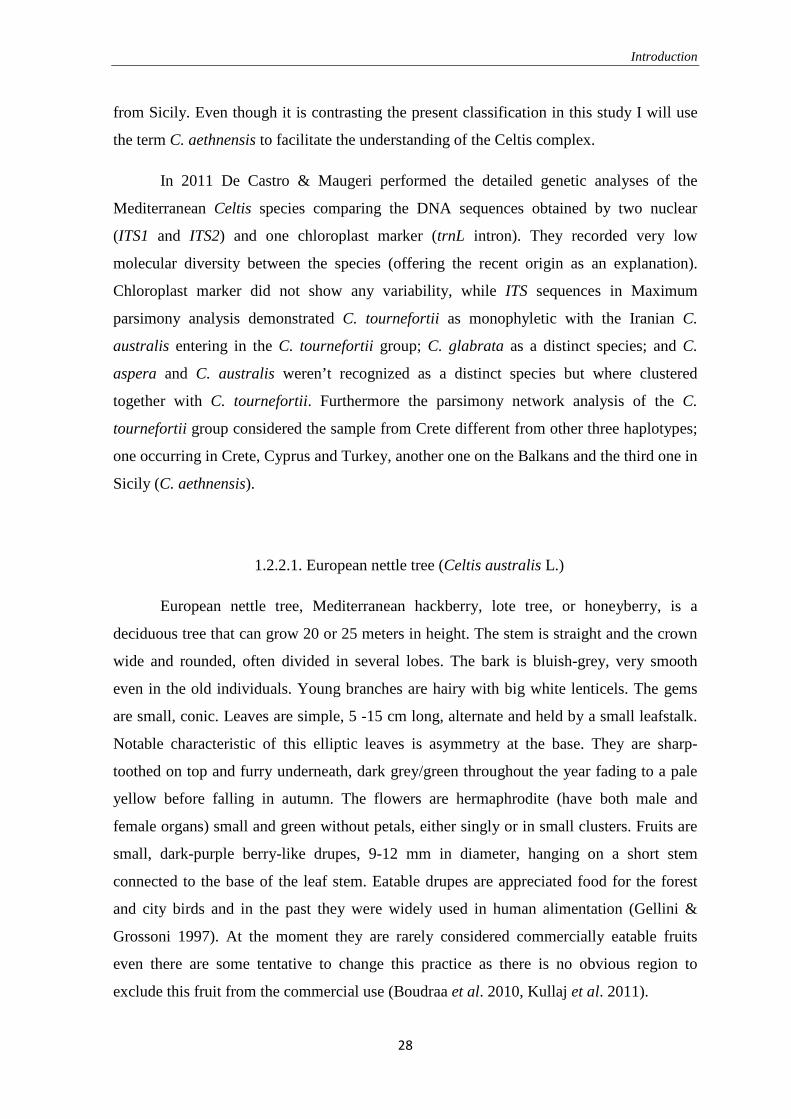
1.2.2.1. European nettle tree (Celtis australis L.)
European nettle tree, Mediterranean hackberry, lote tree, or honeyberry, is a
deciduous tree that can grow 20 or 25 meters in height. The stem is straight and the crown
wide and rounded, often divided in several lobes. The bark is bluish-grey, very smooth
even in the old individuals. Young branches are hairy with big white lenticels. The gems
are small, conic. Leaves are simple, 5 -15 cm long, alternate and held by a small leafstalk.
Notable characteristic of this elliptic leaves is asymmetry at the base. They are sharp-
toothed on top and furry underneath, dark grey/green throughout the year fading to a pale
yellow before falling in autumn. The flowers are hermaphrodite (have both male and
female organs) small and green without petals, either singly or in small clusters. Fruits are
small, dark-purple berry-like drupes, 9-12 mm in diameter, hanging on a short stem
connected to the base of the leaf stem. Eatable drupes are appreciated food for the forest
and city birds and in the past they were widely used in human alimentation (Gellini &
Grossoni 1997). At the moment they are rarely considered commercially eatable fruits
even there are some tentative to change this practice as there is no obvious region to
exclude this fruit from the commercial use (Boudraa et al. 2010, Kullaj et al. 2011).
Introduction
29
The plant prefers light soils, medium nutritive, dry and sub-acid. It is highly
tolerant to the rocky substrates thanks to its strong root and adapted to drought periods. It
is a long-living species (can arrive to the age of 500-600 years) with a slow growing rate.
European nettle tree is a eurimediterranean species with the center of the
distribution in the oriental side spreading from the northern Africa, over Spain, France,
Italy and Balkan Peninsula through whole Anatolia till Kashmir. In Mediterranean it is
found in the broadleaf termophylic forests of Laurus and Castneum (Gellini & Grossoni
1997). Recently Simchoni & Mordechai (2010) discussed its native origin in the Levant.
Apparently recent archaeobotanical findings of Nettle Tree from two Iron Age sites in
Israel indicate that it might be native to Israel-Jordan, but it is still under the discussion and
anticipation of new evidence. The wide usage (fruits and wood) and importance
(traditional beliefs considered it a tree which protects from the bad spirits) of this tree
makes it hard to assure that it wasn’t introduced in the present locations.
The importance of this tree continues till now when it is a very common ornamental
tree in Mediterranean cities. It is slow-growing, resistant and seems to be well resistant on
the pollution of the city (Whittenberghe et al. 2013).
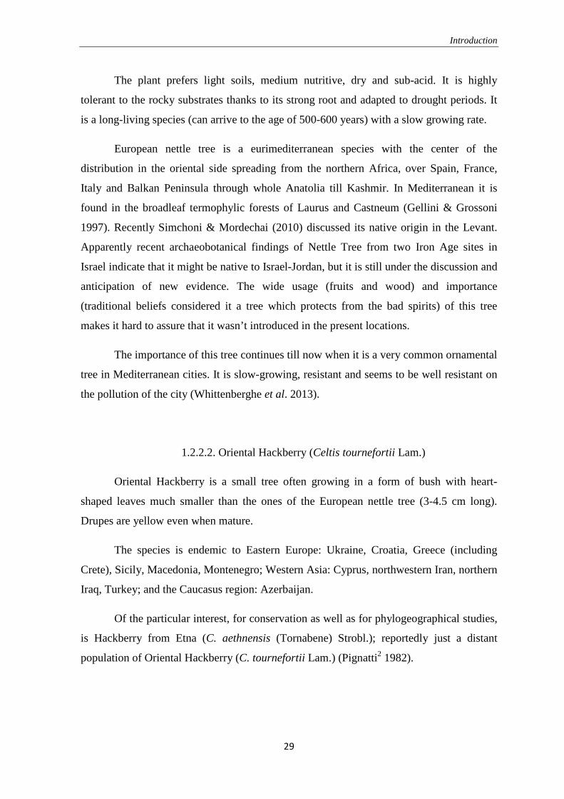
1.2.2.2. Oriental Hackberry (Celtis tournefortii Lam.)
Oriental Hackberry is a small tree often growing in a form of bush with heart-
shaped leaves much smaller than the ones of the European nettle tree (3-4.5 cm long).
Drupes are yellow even when mature.
The species is endemic to Eastern Europe: Ukraine, Croatia, Greece (including
Crete), Sicily, Macedonia, Montenegro; Western Asia: Cyprus, northwestern Iran, northern
Iraq, Turkey; and the Caucasus region: Azerbaijan.
Of the particular interest, for conservation as well as for phylogeographical studies,
is Hackberry from Etna (C. aethnensis (Tornabene) Strobl.); reportedly just a distant
population of Oriental Hackberry (C. tournefortii Lam.) (Pignatti2 1982).

Introduction
30
1.2.3. Inula verbascifolia subsp. verbascifolia
Genus Inula consists of about 100 species dispersed on north hemisphere (Europa,
Asia and North Africa). In Europe have been recorded 19 species. They are all perennial
(rarely biennial) herbs or small shrubs. Leaves are simple and alternate and capitula can be
solitary or in a corymbose or paniculate inflorescence. Florets are yellow, tubular ones are
hermaphrodite and outer, ligulate are female. Popus hairs are simple and free (Ball & Tutin
1964).
Lot of attention has been paid to Inula species due to their diverse biological
activities, particularly in bactericidal, hepatoprotective, and antitumor application (Jiangsu
New Medicine College 1977). This biological significance has prompted phytochemists to
investigate the chemical constituent of Inula plants, which has led to the identification of
many bioactive compounds including monoterpenoids, sesquiterpenoids, flavonoids, and
glycosides (Zhao et al. 2006). Inula species have been used also as traditional herbal
medicines through the world: they have been reported to possess expectorant, antitussive,
diaphoretic, and bactericidal properties (Editorial Committee of the Administration Bureau
of Chinese Flora 1979) and are used in the treatment of inflammation, bacterial and viral
infections (including hepatitis), as well as cancers (Jiangsu New Medicine College 1977).
Especially interesting group of Inula is Inula candida group (figure 1.8), also
noticed for its medicinal properties. It is characteristic for its illiric (amphi-adriatic)
distribution. Plants are usually densely white - tomentose or white - lanate perennials living
in arid places on the limestone stones or cliffs often close to the sea. Three principal
species inside the group are I. candida (L.) Cass., I. verbascifolia (Willd.) Hausskn. and I.
subfloccosa (Rech.). I. subfloccosa is endemic plants included in the IUCN catalogue for
the rare and threatened species of Greece (IUCN 1982) and its areal is not well known.
Other two species are common and consist of numerous subspecies.
Inside I. candida (sin. I. candida subsp. limonifolia (Sibth.& SM.) Hayek) three taxa
are currently recognized:
• candida subsp. candida (western Crete),
• candida subsp. decalvans (Halácsy) P.W. Ball ex Tutin (eastern Crete) and
• candida subsp. limonella (Heldr.) Rech. (central, southern and eastern Greece).

Introduction
31
I. verbascifolia is a plant with slightly higher steam (around 50 cm) inhabiting wider
territory then I. candida. Also here several taxa have been described.
• I. verbascifolia subsp. parnassica (Boiss. & Heldr.) Tutin (central and southern
Greece)
• I. verbascifolia subsp. methane (Hausskn.) (central and southern Greece)
• I. verbascifolia subsp. heterolepis (Karpathos, eastern Greece)
• I. verbascifolia subsp. aschersoniana (Jank) Tutin (Greece, Bulgaria and
Macedonia)
• I. verbascifolia subsp. verbascifolia
Figure 1.8. Distribution of Inula candida group taxa.
I. verbascifolia subsp. verbascifolia is the most widely distributed subspecies,
inhabiting Peninsula Gargano (southern Adriatic coast), northern Adriatic coast and north-
western Balkan Peninsula. It is 20-50 cm tall lanate plant. Basal leaves are ovate-
lanceolate, shortly cuneate at base, 6-9 x 2,5-4 cm big, with veins prominent beneath. Stem
holding the flowers sometimes has few small sessile leaves. Inflorescence (capitulum)
consists of yellow ligulate and tubular flowers. Ligules are 15 mm big, exceeding the
involucres by 2 mm or more. Plant grows on the carsick rocks and flowers in July and
August.
Introduction
32
I. candida group has never been studied on the molecular level, so it is interesting
to see its genetic diversity, genetic distances between the particular taxa and to verify the
similarity of the I. verbascifolia subsp. verbascifolia’s populations which have such a
disjunct distribution.
1.3. Molecular analyses
1.3.1. Discovering the variability and evolutionary history of the species
Differences between the living organisms can be observed in two different temporal
scales: macroevolution (phylogeny) that observes relationships between different species,
so it hypothesizes the past events between the present species based on the current
characters (therefore there is no genetic flow between those species) and microevolution
(genetic population) that observes the events occurring inside one species (gene flow is the
main trait in these studies) trying to find stratification of individuals that are more related
then others.
Exploration of the evolutionary history of the species (phylogeny) and their extant
distances can be performed using various methods. The oldest method for was proposed by
Charles Darwin, father of genetics, who designed the first phylogenetic tree and founded
the theory that species are result of the natural selection and change over the time. Based
on his theory the evolutionary traits of the species should be discovered by comparing their
particular morphological characters (e.g. reproductive system in higher plants).
Morphology studies are still the basic method even though, during the years, various
methods have been introduced in this field. During the late 19th century, Ernst Haeckel
offered a new theory about evolution studies stating that "ontogeny recapitulates
phylogeny" meaning that the development of an organism successively mirrors the adult
stages of successive ancestors of the species to which it belongs. This theory was rejected
after being proofed to be wrong and studies on evolution of the species had to search for
new methodology once again. Cytogenetics, study concerning the structure and function of
the cell (especially the chromosomes), brought numerous results. In the 1980s big
advances were made in molecular cytogenetics when the fluorescent labeled probes started
to be used in the method called fluorescence in situ hybridization (FISH). This technique is
nowadays still very useful for deducing evolutionary relationships between the species.

Introduction
33
Species distances can also be estimated with various biochemical markers; terpenoids
(Hanover 1992, Welter et al. 2012), isozymes (allozymes) (Micales & Bonde 1995,
Filppula et al. 1992, Chunxiao et al. 1999) and proteins (Schirone et al. 1991). The branch
of phylogeny that analyses hereditary molecular differences, mainly in DNA sequences, is
called molecular phylogenetics and its main goal is to show the probable evolution of
various organisms.
Turning to the microevolution, another type of studies often use the similar
methods and technology to discover the current reports inside the species. Population
genetics is the study of allele frequency distribution and its change under the influence of
the main evolutionary processes (natural selection, genetic drift, non-random mating,
mutation and gene flow). It also takes into account the factors of recombination, population
subdivision and population structure. Basically, population genetics attempts to explain
such phenomena as adaptation and speciation. Phylogeography is a study which, by
considering historical geological, climatic and ecological conditions, tries to explain
current distribution of species. Since 1987, when Avise introduced the term
phylogeography (in the article: Intraspecific Phylogeography: The Mitochondrial DNA
Bridge Between Population Genetics and Systematics), another closely related field has
been developed called landscape genetics. While phylogeography investigates the
historical processes generating patterns of genetic variation (Avise et al. 1987), landscape
genetics examines the contemporary processes affecting genetic variation (Storfer et al.
2007). A clear partition between these two scientific domains and the methods that should
be used are still a topic of discussion (Wang 2010, Bohonak & Vandergast 2011, Wang
2011).
The basis of all these studies is DNA sequence. For studying differences in the
DNA sequence various methods have been found. They can be divided in the methods
obtaining the variability by hybridization of the particular DNA part (RFLP) or by
multiplying it in the PCR machine (RAPD, AFLP, microsatellite analysing or DNA
sequencing).
• RFLP (restriction fragment length polymorphism) is a technique that exploits
variations in homologous DNA sequences using the restriction enzymes that cut the
DNA sample according to its DNA sequence. The produced restriction fragments
Introduction
34
are separated, according their lengths in gel electrophoresis. RFLP analyses were
the first DNA profiling technique inexpensive enough to see widespread
application.
Development of the PCR, polymerase chain reaction, (in 1983 by Kary Mullis)
opened the new door to DNA-based analyses and is, nowadays, an essential part of any
phylogenetic or biogeographical study. PCR is a biochemical technology able to amplify a
single, or few copies, of the part of DNA generating thousands to millions of copies of that
particular DNA sequence part.
• RAPD (random amplification of polymorphic DNA) is a type of PCR reaction
where the segments of DNA are amplified randomly. The primers used in this
reaction are short (8–12 nucleotides) and, therefore, manage to be amplified in
many positions and make various fragments of DNA. These fragments are later
observed in gel electrophoresis.
• AFLP is another PCR method which uses restriction enzymes to digest genomic
DNA, followed by ligation of adaptors to the sticky ends of the restriction
fragments. A subset of the restriction fragments is then selected by the primers
complementary to the adaptor sequence, multiplied and these amplified fragments
are separated and visualized on denaturing polyacrylamide gels.
• Microsatellites (also known as Simple Sequence Repeats (SSRs) or short tandem
repeats (STRs)) are repeating sequences of 2-6 base pairs of DNA often presenting
high levels of inter- and intra-specific polymorphism, particularly when the number
of repetitions is 10 or greater. That is why they are ideal for determining paternity,
population genetic studies and recombination mapping. They can be amplified in
the PCR process producing enough DNA to be visible on agarose or
polyacrylamide gels (in which, once again, different lengths are visible due to the
different traveling speed). With the abundance of PCR technology, primers that
flank microsatellite loci are simple and quick to use but the development of
correctly functioning ones is often a costly process (since they are located in the
high variable region of DNA chances that one primer works in a broad spectrum of
species is low).
• DNA sequencing is the process of determining the precise order of nucleotides in
the individual gene, larger genetic regions, full chromosomes or entire genomes.

Introduction
35
The resulting sequences may be used by researchers in molecular biology or
genetics or may be used by medical personnel to make treatment decisions or aid in
genetic counseling. Sequencing can be performed in any part of the DNA so the
sequencing position depends on the result one wants to obtain. The part that is
about to be sequenced is multiplied with standard PCR procedure using the
specialized primers. In this case the primers are usually less taxa-specific so they
can be used for a wide range of organisms. The first DNA sequences were obtained
in the early 1970s using laborious methods based on two-dimensional
chromatography, which was followed by numerous, cheaper and automated
methods. Sanger sequencing is a method based on the selective incorporation of
chain-terminating dideoxynucleotides (ddNTP) by DNA polymerase during in vitro
DNA replication. The ddNTPs may be radioactively or fluorescently labeled so that
their incorporation becomes detected in automated sequencing machines which
record the correct sequence of DNA. It has been the most widely-used sequencing
method for approximately 25 years and still remains common for smaller-scale
projects and for obtaining especially long contiguous DNA sequence reads (>500
nucleotides). One of the most recent methods (first published in 2009) is single
molecule real time sequencing (SMRT), being performed on a single molecule of
DNA as a template. In the contrast of the old methods where chain-terminating
dideoxynucleotides were used to stop the DNA polymerase in SMRT technique
each of the four DNA bases is attached to one of four different fluorescent dyes. As
nucleotides are being incorporated by the DNA polymerase a detector keeps
recording the fluorescent signal of the nucleotide incorporation, making the
sequencing process cheaper and faster.
The basic difference between the last two methods (microsatellite analyses and DNA
sequencing), nowadays also the most used ones, is in the level of polymorphism.
Microsatellites are more variable, as the polymorphism that occurs has a very low impact
on the organism, which makes them perfect for population genetic studies (Agarwall
2008). DNA sequencing is usually made in the less variable zones of DNA, whose
differences have higher significance for the evolution. DNA sequencing is looking for
single-nucleotide polymorphisms (SNPs), DNA sequence variations occurring on a single
nucleotide in the genome. The genomic distribution of SNPs is not homogenous; they

Introduction
36
usually occur in non-coding regions more frequently than in coding regions of DNA. SNPs
frequency also differs between the species and families so there are more and less
conservative taxa. Due to their lower frequency they are much more suitable for the
phylogeny and phylogeographic analyses and their variability can show the direction or the
pattern of the genotype evolution. Also the sampling model is different. While for the
microsatellite analyses many samples are requested (10-20) due to the common diversity
inside the population, DNA sequencing can be performed using one to three samples from
the population (as the possibility of the intra-population diversity is usually low).
1.3.2. Molecular markers used for DNA sequencing
There are three types of DNA genomes present in the plant cells; plastidial (cpDNA),
mitochondrial (mtDNA) and nuclear one. Nuclear genome is diploid and its inheritance is
mendeliana (or biparental), inheriting the DNA from both, mother and father;
mitochondrial genome is haploid, and its inheritance is uniparental coming from the
mother; as well as the plastid one, coming mostly from the mother’s DNA but, in rare
cases as Gymnosperms, from the father.
From the beginning of the phylogeny studies the big interest has been put on the
plastid DNA. Animal systematics has always been based on the mitochondrial genome
which is relatively small (15-19 kb in most of the animals) and highly conserved making it
perfect for population genetics and taxonomy studies. The plant mitochondrial genome is
much different from the animal one. Plant genome is considered less informative as well as
highly variable in size, structure and gene order. Recently more and more studies have
been conducted using the mitochondrial DNA sequences and they have shown that the
high variability under some groups can be a useful characteristic for systematics analyses.
In 2010 Qiu et al. carried out the angiosperm phylogeny study inferred from sequences of
four mitochondrial genes and in conclusion states that several potential problems of
mitochondrial genes such as heterogeneity rate, horizontal DNA transfer and RNA editing
have been somewhat exaggerated and can be effectively dealt with selective taxon
sampling and analysis of combined multigene datasets. They also think that, in order to
understand angiosperm phylogeny (up till now extremely concentrated to chloroplast DNA
analyses), it is essential to develop its independent hypotheses using information from

Introduction
37
mitochondrial and nuclear genes. The proof of usefulness of mtDNA sequences can be
found in many specialized phylogenetic studies as the one of the Begoniaceae phylogeny
(Goodall-Copestake et al. 2010) where the number of parsimony informative sites in the
mitochondrial sequence was higher even though the sequence was shorter and the total
number of variable cites was lower. The article states that there have been found the
conflicts between the chloroplast and mitochondrial cladograms but they only suggest that
additional evolutionary important processes may also have occurred.
In plant phylogeny ribosomal DNA (nrDNA) is the most used part of the nuclear
DNA. The major ribosomal RNA genes of plants are localized in clusters of highly
repeated sequences, each repeat consisting of sequences for the 18S, 5.8S, and 28S
ribosomal subunits (figure 1.9). These genes show little sequence divergence between
closely related species. Within each repeat, these conserved regions are separated by
internal transcribed spacers (ITS), which show higher rates of divergence. The designation
for the spacer between the 18S and 5.8S genes is “ITS1”; the designation for the spacer
between the 5.8S and 28S genes is “ITS2”. A third spacer, the large intergenic spacer
(IGS), is found between the 3’ end of the 28S and the 5’ beginning of the 18S genes. Both
internal transcribed spacer regions (ITS1 and ITS2) of 18S-28S nuclear ribosomal DNA
(nrDNA) were proved as a useful source of characters for phylogenetic studies at various
taxonomic levels in many angiosperm families (Baldwin et al. 1992).
Figure 1.9. Nuclear ribosomal RNA gene cluster.
Chloroplast DNA sequences are the most studied and recommended till now (figure
1.10). Early in the plant molecular systematics history chloroplast DNA (cpDNA) was
surveyed through restriction site polymorphism studies (Olmstead & Palmer 1994) and it
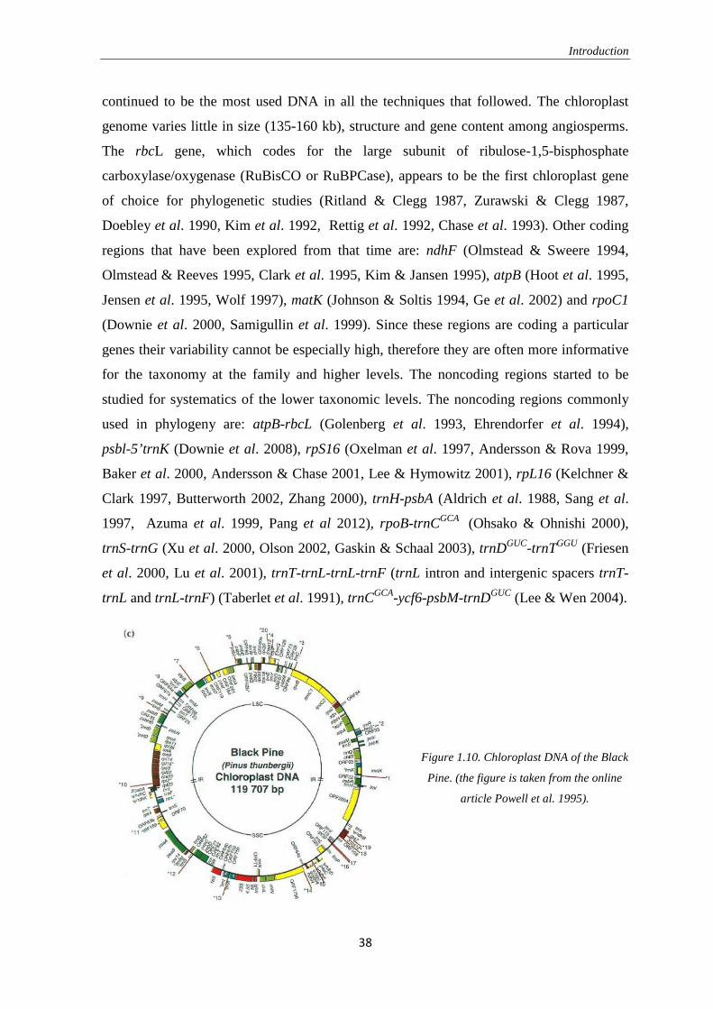
Introduction
38
continued to be the most used DNA in all the techniques that followed. The chloroplast
genome varies little in size (135-160 kb), structure and gene content among angiosperms.
The rbcL gene, which codes for the large subunit of ribulose-1,5-bisphosphate
carboxylase/oxygenase (RuBisCO or RuBPCase), appears to be the first chloroplast gene
of choice for phylogenetic studies (Ritland & Clegg 1987, Zurawski & Clegg 1987,
Doebley et al. 1990, Kim et al. 1992, Rettig et al. 1992, Chase et al. 1993). Other coding
regions that have been explored from that time are: ndhF (Olmstead & Sweere 1994,
Olmstead & Reeves 1995, Clark et al. 1995, Kim & Jansen 1995), atpB (Hoot et al. 1995,
Jensen et al. 1995, Wolf 1997), matK (Johnson & Soltis 1994, Ge et al. 2002) and rpoC1
(Downie et al. 2000, Samigullin et al. 1999). Since these regions are coding a particular
genes their variability cannot be especially high, therefore they are often more informative
for the taxonomy at the family and higher levels. The noncoding regions started to be
studied for systematics of the lower taxonomic levels. The noncoding regions commonly
used in phylogeny are: atpB-rbcL (Golenberg et al. 1993, Ehrendorfer et al. 1994),
psbl-5’trnK (Downie et al. 2008), rpS16 (Oxelman et al. 1997, Andersson & Rova 1999,
Baker et al. 2000, Andersson & Chase 2001, Lee & Hymowitz 2001), rpL16 (Kelchner &
Clark 1997, Butterworth 2002, Zhang 2000), trnH-psbA (Aldrich et al. 1988, Sang et al.
1997, Azuma et al. 1999, Pang et al 2012), rpoB-trnCGCA (Ohsako & Ohnishi 2000),
trnS-trnG (Xu et al. 2000, Olson 2002, Gaskin & Schaal 2003), trnDGUC-trnTGGU (Friesen
et al. 2000, Lu et al. 2001), trnT-trnL-trnL-trnF (trnL intron and intergenic spacers trnT-
trnL and trnL-trnF) (Taberlet et al. 1991), trnCGCA-ycf6-psbM-trnDGUC (Lee & Wen 2004).
Figure 1.10. Chloroplast DNA of the Black
Pine. (the figure is taken from the online
article Powell et al. 1995).

Introduction
39
Most of the analyses recently conducted tend to include more markers possible in
order to get more confirmations on their assumption. The combinations are various and
there is no rule about better region. The informativity of the markers varies from genus to
genus and it is often necessary to test numerous markers to find the most informative one.
Observing great number of phylogeny analyses there are still some trends to notice about
the marker combinations researchers use. Kajita et al. in 1998 analyzed phylogeny of
Dipterocarpaceae using the nucleotide sequences of matK, trnL intron, and trnL-trnF.
Asmussen & Chase in 2001 studied palm systematic using the rps16 and trnL-F seqences.
In 2002 Bayer et al. used trnL intron, trnL-trnF, matK, and ETS for resolving the
phylogeny of Australian Gnaphalieae (Asteraceae); Cuénoud et al. (2002) tried to resolve
the phylogeny of Caryophyllales with the nuclear 18S rDNA and plastid rbcL, atpB, and
matK DNA sequences; while Mast & Guivnish (2002) studied biogeography under the
family Proteaceae using trnL intron, trnL-trnF, rp116 intron, psbA-trnH and trnT-trnL
spacers. In 2003 Samuel et al. analyzed phylogenetic relationships among species of
Hypochaeris (Asteraceae, Cichorieae) using ITS, trnL intron, trnL-trnF and matK
sequences; Vinnersten & Reeves studied the phylogenic rapports within Colchicaceae with
rps16, atpB-rbcL and trnL-F sequences; and Miller et al. analyzed phylogeny of
Mimosoideae using trnK, matK, psbA-trnH, and trnL-trnF sequences. More recently, in
2012, there is a great variety in markers being used for phylogenetic analyses; Chemisquy
& Morrone studied the molecular phylogeny of Gavilea (Chloraeinae: Orchidaceae) using
the rpoC1, matK-trnK and atpB-rbcL plastid markers and the nuclear marker, ITS; Chen et
al. analyzed phylogeny and biogeography of Alismataceae with nuclear: ITS, chloroplast:
psbA, rbcL, matK, rpoB, rpoC1, trnK 5' and trnK 3', and mitochondria: cob and atp1
markers; Weng et al. studied the phylogeny, rate variation, and genome size evolution of
Pelargonium (Geraniaceae) with plastid (rbcL, matK, ndhF, rpoC1, trnL-trnF) and
mitochondrial (nad5) genes; Li et al. analyzed molecular phylogeny of Ficus section Ficus
obtaining the trnH-psbA, psbK-psbI and atpF-atpH sequences. Based on these studies
conclusions to be taken are:
- more markers are being used in a single study and
- mitochondrial sequences are being more often used.
Introduction
40
Despite the great variability of the regions used in studies it is still possible to make
certain conclusions about the best regions to use in the study. Several noncoding cpDNA
regions, such as the commonly employed trnL-trnL-trnF and trnK-matK, are identified to
consistently provide greater levels of sequence variation compared to other regions that
consistently yield low levels of variation (Shaw et al. 2007). Heider & Wilkinson (2010)
generated 84 new universal primers in order to test their variability and showed that the
most variable were: rpl23&rpl2.1, 16S, 23S, 4.5S&5S, petB&D, rpl2, rpoC1 and trnK. In
2012 Dong et al. scanned the entire chloroplast genomes of 12 genera once again searching
for highly variable regions. The order of the regions from the most to the less variable was
following: ycf1-a, trnK (including matK), rpl32-trnL, trnH-psbA, trnSUGA-trnGUCC,
petA-psbJ, rps16-trnQ, ndhC-trnV, ycf1-b, ndhF, rpoB-trnC, psbE-petL and rbcL-accD.
Another consideration to take when choosing the primers for a study is the number of
studies in which this region has been used till know. Regularly analyzed regions are rich
with the sequences in the DNA banks, which gives the opportunity to confirm or test the
result obtained. Eventually the sequences from the DNA bank could be included in the
study in order to enrich the analysis and arrive to stronger supported result. DNA
barcoding is a molecular tool the most dependent on the good and reliable database. As the
number of DNA barcode sequences increases, data exchange becomes more complicated
and the need of a comprehensive database rises as well. As often this technique analyses
the same regions of chloroplast DNA, its banks and databases can be used as a complement
to biosystematics, biodiversity, phylogenetic and phylogeography reconstructions
(Hajibabaei et al. 2007). The global DNA database used mostly at the moment is the one
located at the National Center for Biotechnology Information site;
http://www.ncbi.nlm.nih.gov.
Chloroplast and nuclear DNA markers used in this study are the most used and
recommended ones therefore it was expected that their sequences will be also well
represented in the NCBI GenBank.
The trnHGUG-psbA intergenic spacer region was first described by Aldrich et al.
(1988) who showed that indels were prevalent in this region, even between closely related
species from the Fabaceae and Solanaceae family. An early study that showed this region
to be of value to systematics is performed by Sang et al. (1997) who noted that it was
highly variable compared to matK and trnL-trnF. Many studies followed this example and

Introduction
41
used the region for studying closely related genera and species (Azuma et al. 1999,
Chandler et al. 2001, Fukuda et al. 2003, Miller et al. 2003, Tate & Simpson 2003), or also
for intra specific investigations (Holdregger & Abbott 2003). Although studies have shown
that trnH-psbA contains a very high percentage of variable characters (Azuma et al. 2001,
Piredda et al. 2011) this spacer is usually coupled with other regions because it is
comparatively short and may not yield enough characters with which to build a well-
resolved phylogeny. The average length of trnH-psbA is 465 bp, and it ranges from 198 to
1077 bp (Shaw 2007). The region sometimes contains several poly A/T structures that can
cause problems in sequencing. Among more distantly related taxa, this indel prone middle
region may generate a relatively high amount of homoplasy due to apparent indel ‘‘hot
spots’’ with numerous, repeating, and overlapping indels.
The matK gene region is located within an intron of the chloroplast trnK gene,
(psbA-39trnKUUU-[matK]-59trnKUUU). Several studies have used the entire trnK-matK-trnK
region (Johnson & Soltis 1994, Hardig et al. 2000, Miller & Bayer 2001), while most have
carved out various portions of this 2600 bp long region. Only the matK region is
approximately 1500 bp long but the part that is being usually sequenced in the studies
varies due to big number of the primers used. The matK region is usually being used for
the studies below family level (Kim et al. 2007, Kajita et al. 1998, Bayer et al. 2002,
Cuénoud et al. 2002, Ge et al. 2002, Samuel et al. 2003) but it has also been suggested as
an effective tool for higher levels (Hilu & Liang 1997, Hilu et al. 2003). The biggest
problem with this region is the absence of the universal primers, due to the variability of
the gene across broad phylogenetic lineages. Often specific primers have to be made for
the studied group (Wang et al. 1999, Hardig et al. 2000, Miller & Bayer 2001, Mort et al.
2001, Pridgeon et al. 2001, Bayer et al. 2002, Hilu et al. 2003), which make the usage of
this region relatively expensive.
The first study to use the trnSGCU-trnGUUC region was the study of population
dynamics within tropical tree species in Corythophora (Lecythidaceae) and subsequently
published the primers along with the suggested amplification protocol. Xu et al. (2000)
designed nearly the same primers for this spacer for use in Glycine (Fabaceae). Subsequent
studies have shown this region to be highly variable (Xu et al.2000, Olson 2002, Sakai et
al. 2003, Olson 2002, Perret et al. 2003). The trnS-trnG spacer is in average 763 bp long
and ranges from 619 to 1035 bp. Sometimes, as is the case in Taxodium, this poly-A/T run
Introduction
42
is over 30 bp and prohibits sequencing from that direction (Shaw et al. 2007). Because of
independent structural rearrangements in both monocots (Hiratsuka et al. 1989) and
Asteraceae, excluding Barnadesieae (Jansen & Palmer 1987), the trnS-trnG spacer does
not exist in these taxa.
Chloroplast trnS–trnQ intergenic spacer is located in the large single-copy region of
the plastid genome, between trnS and trnQ genes. The first primers designed in this region
were the ones of Kanno (2004) made for analsyis of four Quercus species in Japan. In this
study trnQ-trnS was the only variable region between the following: trnDT, trnTL,
rps14psaB, trnST-1 and trnST. The same primers have been later used in other studies on
the genera Quercus (Zeng et al. 2011, Liu & Harada unpublished). In 2010 Schirone et al.
designed the primers for the same region to be used on a study of genus Taxus. This region
was chosen because Hao et al. (2008) found this fragment able to discriminate among 14
Old World and New World Taxus species. The primers were designed based on selecting
the most variable region in the spacer (located between 225 and 901 bp).
The trnTUGU-trnLUAA-trnLUAA-trnFGAA is set in a region comprising three tRNA genes
trnTUGU, trnLUAA, and trnFGAA. The noncoding portions of the region include intron that
interrupts the trnL gene, as well as the intergenic spacers between trnT-trnL and trnL-trnF,
and these are the parts usually being sequenced. One of the first sets of universal PCR
primers for non-coding cpDNA was published by Taberlet et al. (1991). The set consist of
three primer pairs even though sometimes sequencing can be performed using just the first
and the ultimate of them. Because of the near-universal nature of the primers and their
early publication, these regions have become the most widely used noncoding cpDNA
sequences in plant systematics. Already in December 2003, Web of Science listed 579
citations of the Taberlet et al. (1991) paper. Slight problems seemed to have shown the
trnT primer (Taberlet et al. 1991, primer ‘‘A’’) so Cronn et al. (2002) designed a new one
that has been in use since then. Usually these regions are employed in studies of closely
related species or genera, but a recent study by Borsch et al. (2003) used the entire region
to evaluate relationships among basal angiosperms. These three regions are sometimes
used all together (Bremer et al. 2002, Yang et al. 2002, Downie et al. 2002, Bremer et al.
2002, Demaio et al. 2011) or just some parts. When used partially trnT-trnL intergenic
spacer (Cronn et al. 2002, Applequist & Wallace 2002, Fehrer et al. 2009) makes the
sequences from 400–1500 bp long and often including large A/T rich regions; trnL intron

Introduction
43
(Gielly & Taberlet 1994, Goldblatt et al. 2002, Mast & Givnish 2002) makes the sequences
250-1400 bp long; and trnL-trnF spacer (Stech et al. 2003, Bellstedt et al.2001, Gielly &
Taberlet 1994, Sang et al. 1997, Mort et al. 2001, Goldblatt et al. 2002, Borsch et al. 2003,
Fukuda et al. 2003, Jobson et al. 2003, Miller et al. 2003, Salazar et al. 2003, Simpson et
al. 2003, Bellstedt et al. 2001) produces the sequences 100-500 bp long.
When studying the nuclear genome, the internal transcribed spacer (ITS1 and ITS2)
sequences of 18S–28S nrDNA are the ones most commonly used to assess plant
phylogenetic relationships. For the first time this region was used in a phylogenetic study
already in 1992 (Baldwin) and 1993 (Baldwin) and since then it has been in continuous
use. Álvarez & Wendel stated in 2003 that from 244 phylogenetic publications during the
last five years in several of the most prominent systematics and evolution journals, two-
thirds (66%) involving comparisons at the genus level or below included ITS sequence
data. Another even more striking fact they discovered is that more than one third (34%) of
all published phylogenetic hypothesis have been based exclusively on ITS sequences. This
region has been successfully used for obtaining good results at the intergeneric level
(Baldwin 1992, Suh et al. 1993, Martinez-Azorin 2011, Inda et al. 2012, Wheeler et al.
2013) as well as on the intrageneric level (Baldwin 1993, Ritland et al. 1993, Kim &
Jansen 1994, Gielly et al. 1996, Ocampo & Columbus 2012, Su et al. 2012). The length of
the amplified fragment including ITS1, ITS2, and 5.8S rDNA, is typically less than 700
nucleotides (longer in gymnosperms). As being highly conservative region a set of primers
designed in 1990 by White et al. was useful for amplifying ITS sequences from most plant
and fungal phyla. Exactly this universality has been sometimes recorded as a defect
because the high universality of the amplification primers commonly used increase the
possibility of contamination of the reaction cocktail with tissue from different plants (or
even a fungus). Other problems occurring at ITS based phylogeny studies are caused by the
fact that 18S–5.8S–28S repeats exist in hundreds to thousands of copies at one or more
than one chromosomal location. Since the arrays are so many and often evolutionarily
labile it is theoretically possible to find the evolved arrays inside the same organism. Some
of them could be so different that they are not even functional any more, but instead have
degenerate into pseudogenes. This could cause errors and misinterpretations of the results
so Álvarez & Wendel (2003) consider necessary that ITS stops being routinely utilized
region, substituting it by several or more different single-copy nuclear loci. While in
Introduction
44
angiosperms ITS1 and ITS2 are usually being used together, ITS1 in gymnosperms is very
long (due to long repeating part) so it usually becomes hard for sequencing. This is why
alternative primers should be used when studying gymnosperms. In this study I used the
primer designed in my laboratory by Simeone (unpublished) and it is covering last part of
the ITS1 spacer (last cca 30 bp), spreads over the whole 5.8S RNA and almost the whole
ITS2 spacer.
1.3.3. Molecular phylogenetics
Computational phylogenetics is the application of computational algorithms, methods
and programs on the phylogenetic analyses. Reconstructing the phylogeny from the DNA
sequences is not as straightforward as one might hope, and it is rarely possible to verify
that one has arrived at the “true” conclusion (Vandamme 2009). The goal of all the
phylogeny reconstructions is to assemble a phylogenetic tree or phylogenetic network
representing a hypothesis about the evolutionary ancestry of a set of genes, species, or
other taxa.
Each phylogenetic analysis starts with sequences alignment from homologus regions
(regions that come from a common ancestor). The aim of the multialignment is to find the
real positional homology of residues, therefore to arrange the sequences so that the
homologues bases are aligned together “as much as possible” (Higgis & Lemely 2009). In
this way we can infer evolutionary relationships between the sequences. Very short or very
similar sequences can be aligned by hand but the problem occurs with the long sequences
with many differences. During evolution events of insertions or deletions occur, in
different frequency, especially in non-coding regions. These gaps are highly problematic in
multialignment because they often make impossible to be sure of real positional homplogy
in columns. There are numerous software aides for multiple alignments which tend to
arrange the sequences in order to be as similar as possible in a same time allowing fewer
gaps possible. Some of the most common algorithms that perform a reliable multiple
alignment are MAFFT (Katoh et al. 2002), MUSCLE (Edgar 2004), T-Coffee (Notredame
et al. 2000), ClustalW (Thompson et al. 1994) etc.
After multialignment, phylogenetic tree or network can be made using several
methods. The methods can be divided based on the data they use (discrete character or

Introduction
45
distance matrix) or according to the algorithmic approach of the method, on clustering
algorithm methods and optimality criterion methods.
Distance matrix methods start by calculating the measure of dissimilarity between the
sequences in order to produce a pairwise distant matrix. These distances are then
reconciled to produce a tree (a phylogram, with informative branch lengths). The simplest
way to measure the divergence between two strands is to count the number of sites where
they differ. This method is called the p-distance and, even though, is a very intuitive,
suffers from a strong underestimation of the results as the multiple substitutions on the
same site don’t get recorded (A �G�C = A�C), especially the ones that lead to the
original value (A�G�A = A). Therefore distance-based methods tend to apply several
evolutionary models which will try to estimate the real number of the substitutions that
occurred. A big number of evolutionary models have been proposed differing in terms of
the parameters used to describe the rates at which one nucleotide replaces another during
evolution (De Peer 2009). The use of a particular evolutionary model may change the
outcome of the phylogenetic analysis therefore statistical model selection has become an
essential step for the estimation of phylogenies from DNA sequence alignments (Posada
2008). One of the newest programs able to perform the statistical selection of models of
nucleotide substitution is jModelTest, suggesting the best model for a dataset. The simplest
model is JC69 model (Jukes & Cantor 1969) which assumes the equal bases frequencies
and equal mutation rates. The only parameter of this model, therefore, is the overall
substitution rate. Calculating more parameters and considering the differences between the
bases frequencies and occurrence are other, more complex models as: K80 model (Kimura
1980), F81 model (Felsenstein 1981), T92 model (Tamura 1992), TN93 model (Tamura &
Nei 1993) etc. After deciding the evolutionary model, there is still a method that can be
chosen based on the data that are being analyzed.
Clustering methods
UPGMA (Unweighted Pair Group Method with Arithmetic mean) is the oldest and
simplest method in which clustering is done by searching for the smallest value in the
pairwise distance matrix and the same process is being repeated till all the characters in the
matrix are calculated. This way the process of clustering assumes that the evolution rate is
the same in all branches which does not have necessary to be the case. Minimum evolution
method is trying to construct the tree with the shortest sum of branch lengths (minimizes
Introduction
46
the length of the tree) and thus minimizes the total amount of evolution assumed. Neighbor
Joining (NJ) method is often similar in a result but the method is different. It is the most
commonly used method for constructing the distance trees. This method constructs a tree
by sequentially finding pairs of the neighbors, which are the pairs of the sequences
connected by a single node. The NJ algorithm starts by assuming a star-like tree that has no
internal branches; in the first round finds all the similar to make the first node etc. Even
though it usually brings to very logical tree the basic critic of this method is the lack of any
sort of optimality criterion, and so there is no guarantee that the recovered tree is the one
that best fits the data. Fitch-Margoliash method is another distance-matrix method which,
contrary to all the others, produces more trees and evaluates them to find the one that
minimizes the differences between the pairwise genetic distances and the distances
represented by the sum of branch length for each pair of taxa in the tree.
In order to confirm the results from any of the methods there is always bootstrap consensus
tree with the bootstrap values showed on the tree. This means that the same analysis has
been run many times, bringing big number of phylogenetic trees. From these trees the one
(consensus tree) has been showed demonstrating in how many cases each bifurcation has
been supported (the value showed is the bootstrap). It is a simple and efficient way to test
the relative stability of groups within a phylogenetic tree.
Character-state methods
Character-state methods can use any set of discrete characters (morphological,
physiological, sequence data). After the sequences have been aligned every sequence
position is considered the “character” and every nucleotide at that position is “state”.
Character-state methods are: Maximum parsimony (MP), Maximum likelihood (ML) and
Bayesian inference. All of these methods obtain the results optimizing search criterion,
therefore they all obtain many possible trees from which they choose the most probable
one.
• The basic idea of the maximum parsimony method is seeking to minimize the
amount of evolutionary changes. The approach of minimizing the evolutionary
changes is often considered a right approach even though it is not totally correct
regarding the evolution. MP is often characterized as implicitly adopting the
philosophical position that evolutionary change is rare, or that homoplasy
Introduction
47
(convergence and reversal) is minimal in evolution which is not always the case.
The problem from which this method is suffering is also the so-called “long-branch
attraction” occurring as there is no way to correct for multiple hits (MP assumes
that a common character is inherited directly from a common ancestor and thus
underestimates the real divergence between distantly related taxa). Trees obtained
in the analyses are scored (evaluated) by using a simple algorithm to determine
how many "steps" (evolutionary transitions) are required to explain the distribution
of each character. A step is, in essence, a change from one character state to
another; although with ordered characters some transitions require more than one
step. There are a number of methods for summarizing the relationships within this
set, including consensus trees, which show common relationships among all the
taxa, and pruned agreement subtrees, which show common structure by temporarily
pruning "wildcard" taxa from every tree until they all agree. Reduced
consensus tree takes this one step further, by showing all subtrees (and therefore all
relationships) supported by the input trees.
• Maximum likelihood is similar to the MP in that it examines different tree
topologies and evaluates the relative support by summing over all sequence
positions. ML algorithm searches for the tree that maximizes the probability of
observing the character states, given a tree topology and a model of evolution. It is
a parametric statistical method, in that it employs an explicit model of character
evolution. Likelihood is generally regarded as a more desirable method than
parsimony, in that it is statistically consistent, has a better statistical foundation,
and it allows complex modeling of evolutionary processes. A major drawback is
that ML is still quite slow relative to parsimony methods, sometimes requiring days
to run large datasets.
• Bayesian inference is a method whose goal is to estimate the distribution of a
quantity called the posterior probability of a phylogenetic tree. The posterior
probability of a result is the conditional probability of the result being observed,
computed after seeing a given input dataset. In order to estimate the posterior
distribution probability (which would elsewhere be impossible to commute due to
the enormous number of the tree topologies) Markov chain Monte Carlo sampling,
MCMC, is being used. These algorithms have the property that they converge
towards an equilibrium state regardless the initial point. The algorithm used in for
Introduction
48
such analyses is Metropolis Coupling able to arrive to the stabile state in relatively
short time. The main attraction of Bayesian inference is that it produces distribution
of phylogenetic trees rather than a point estimate, in many cases using less time
than a maximum likelihood analysis followed by a bootstrap analysis (Huson et al.
2010).
Alternative to the phylogenetic trees provide phylogenetic networks which may be
more suitable for datasets whose evolution involve significant amounts of reticulate events
caused by hybridization. A phylogenetic network is any graph used to represents
evolutionary relationships between a set of taxa that labels some of its nodes. Between the
several types of networks (split network, reticulogram, hybridization networks,
recombination networks, DLT networks) the most common is the haplotype network. It is
an unrooted phylogenetic network in which the nodes represent different haplotypes within
a group of (usually very closely related) samples. The edges are usually labeled by the
position at which the joined haplotypes differ. The construction of the haplotype network
starts with the aligned sequences and is obtained using median-joining or reduced median
algorithms. Median-joining algorithm constructs an informative subnetwork of the full
quasi-median network, guided by the minimum spanning network, thus overcoming the
drawbacks of both approaches. The median-joining method is best suited for very closely
sequences that have evolved without recombination and is widely used in phylogeography
and population studies. In reduced median algorithm one attempts to simplify the network
by postulating appropriate parallel mutation events (Huson et al. 2010).
As a conclusion it should be said that all the methods demonstrated have their pros and
cons. All of them are valuable to consider and try, even though they sometimes lead to
slightly different results. While distance matrix methods have to convert the data to the
matrix, character-state methods use the sequence data. Character-state methods therefore
deal with the original data without transforming them and, in that way, are conserving
more information about the sequences. Another difference is between the parametric
(Maximum likelihood, Bayesian inference, Neighbor joining) and non-parametric
(Maximum parsimony) statistical methods. It is generally considered that parametric
methods provide better results as they give wider range of the possibilities to personalize
each dataset, but this is true only if the model used in analysis is a reasonable
approximation of the processes that produced the data. Many critics for example said that

Introduction
49
evolution is a process too complicated to be explained by a model. Other say that this
premise doesn’t necessary mean that a good model cannot be made. Using more
complicated methods requires more sophisticated bioinformatics means which becomes
more time consuming and that is another aspect which sometimes needs to be considered.
Haplotype networks are able to demonstrate small differences between the sequences
(which no phylogenetic tree is able to generate) and this is why it is a priceless instrument
for low variable datasets.

2.Objectives and the scope of study
50
2. OBJECTIVES AND SCOPE OF THE STUDY
In this thesis, four Mediterranean species/species complexes (European Black Pine,
Aleppo Pine, European Nettle Tree and Inula verbascifolia group) were selected to explore
their evolutionary relationships. Apart from being endemic and subendemic in the
Mediterranean Basin, they are interesting due to their disjunct distribution in the
heterogeneous landscape of the Mediterranean peninsulas, islands and mountains. In
addition, taxonomy of the selected taxa is still unresolved and their systematic issues are
ongoing debate (their subspecies, closely related species or disjunct populations).
Systematics based on morphology has been widely studied and generally resolved for all
the studied species. Various biochemical markers have also been applied to some of the
species (European Black Pine), as well as the microsatellites analyses (European Black
Pine and Aleppo Pine). Regardless of the studies carried out so far, a comprehensive
molecular systematics has not been achieved yet. Assessing coherent taxonomic rankings
and confirming current systematics with molecular phylogenetics is a necessary
prerequisite towards more advanced studies concerning phylogeography, species
conservation and activities aimed at habitat restoration.
The aim of this study was:
1. to provide new insights about systematics and phylogeography of the
studied species
In order to assess the comparative genetic variation of the selected taxa chloroplast and
nuclear sequences, from the various DNA regions, were used. Combination of this two
kinds of genetic information (molecular and nuclear) is especially informative for the
phylogeny studies. Studied regions, usually used in, both, phylogenetic and barcoding
studies, come from relatively conserved DNA regions (both coding and non-coding ones
were used), but usually contain a satisfactory quantity of substituted sites and therefore
have a good capacity of underlining evolutionary patterns of investigated taxa.
2. to evaluate different types of DNA markers and different phylogenetic
methods for their applicability and usefulness in taxonomic research
Important side result in the most of the phylogenetic studies is the evaluation of the studied
DNA regions (their applicability and informativity). Thereby, many DNA markers were
2.Objectives and the scope of study
51
tested to test their applicability on the research of these taxa and to provide an objective
judgment about the chosen DNA regions as suitable markers. Computational analyses were
carried out with the same comparative approach. Most of the available methods for
obtaining phylogenetic trees (Neibourgh joining, Maximum likelihood and Bayesian
inference) were tested, as well as use of the phylogenetic networks. All of these methods
were compared in order to present a comprehensive view of the possibilities that
phylogenetic studies offer at the moment.
3. to assess the comparative genetic variation of four Mediterranean taxa
differing in their ecology, biology, life-history traits and distribution
Mediterranean area is a place of great number of biodiversity hot-spots as well as, still
undiscovered, refugia. Any genetic variation inside the species could be a sign of isolation
of a population and therefore can present a precious source of the genetic material of the
species. Finally, genetic variation pattern concordant between different taxa can assess
valuable information about the past events occurring in the Mediterranean Basin.
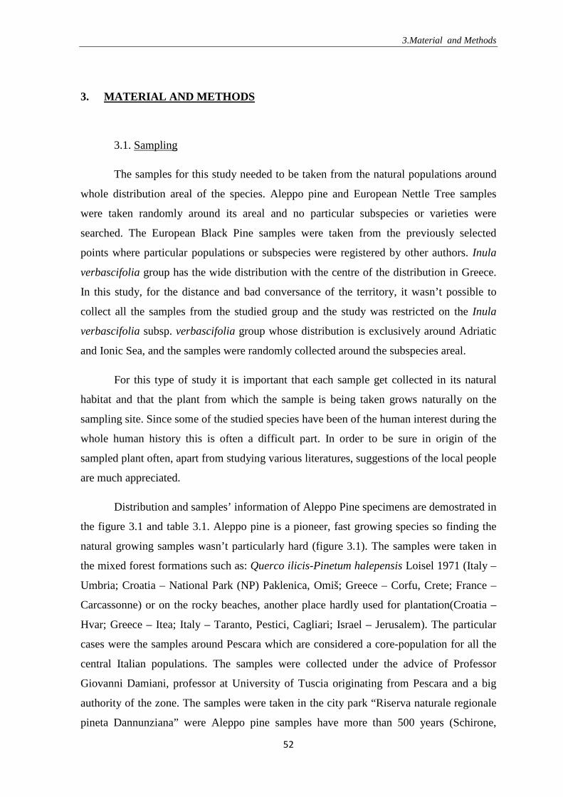
3.Material and Methods
52
3. MATERIAL AND METHODS
3.1. Sampling
The samples for this study needed to be taken from the natural populations around
whole distribution areal of the species. Aleppo pine and European Nettle Tree samples
were taken randomly around its areal and no particular subspecies or varieties were
searched. The European Black Pine samples were taken from the previously selected
points where particular populations or subspecies were registered by other authors. Inula
verbascifolia group has the wide distribution with the centre of the distribution in Greece.
In this study, for the distance and bad conversance of the territory, it wasn’t possible to
collect all the samples from the studied group and the study was restricted on the Inula
verbascifolia subsp. verbascifolia group whose distribution is exclusively around Adriatic
and Ionic Sea, and the samples were randomly collected around the subspecies areal.
For this type of study it is important that each sample get collected in its natural
habitat and that the plant from which the sample is being taken grows naturally on the
sampling site. Since some of the studied species have been of the human interest during the
whole human history this is often a difficult part. In order to be sure in origin of the
sampled plant often, apart from studying various literatures, suggestions of the local people
are much appreciated.
Distribution and samples’ information of Aleppo Pine specimens are demostrated in
the figure 3.1 and table 3.1. Aleppo pine is a pioneer, fast growing species so finding the
natural growing samples wasn’t particularly hard (figure 3.1). The samples were taken in
the mixed forest formations such as: Querco ilicis-Pinetum halepensis Loisel 1971 (Italy –
Umbria; Croatia – National Park (NP) Paklenica, Omiš; Greece – Corfu, Crete; France –
Carcassonne) or on the rocky beaches, another place hardly used for plantation(Croatia –
Hvar; Greece – Itea; Italy – Taranto, Pestici, Cagliari; Israel – Jerusalem). The particular
cases were the samples around Pescara which are considered a core-population for all the
central Italian populations. The samples were collected under the advice of Professor
Giovanni Damiani, professor at University of Tuscia originating from Pescara and a big
authority of the zone. The samples were taken in the city park “Riserva naturale regionale
pineta Dannunziana” were Aleppo pine samples have more than 500 years (Schirone,
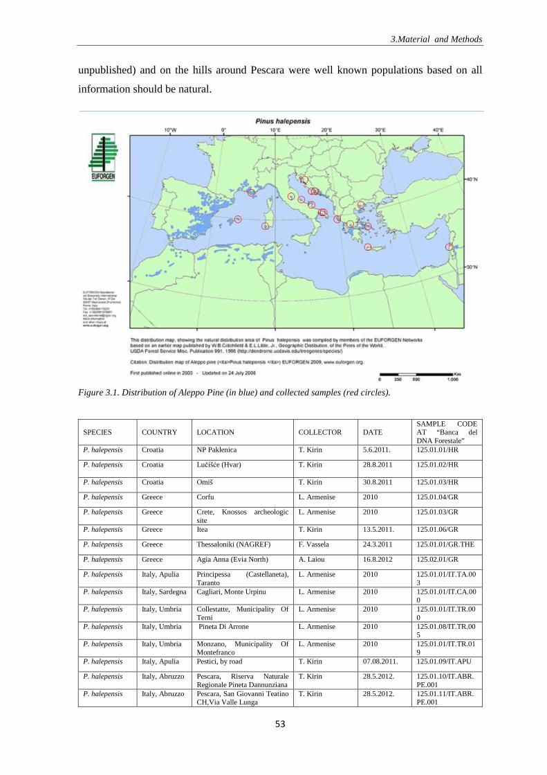
3.Material and Methods
53
unpublished) and on the hills around Pescara were well known populations based on all
information should be natural.
Figure 3.1. Distribution of Aleppo Pine (in blue) and collected samples (red circles).
SPECIES COUNTRY LOCATION COLLECTOR DATE SAMPLE CODE AT “Banca del DNA Forestale”
P. halepensis Croatia NP Paklenica T. Kirin 5.6.2011. 125.01.01/HR
P. halepensis Croatia Lučišće (Hvar) T. Kirin 28.8.2011 125.01.02/HR
P. halepensis Croatia Omiš T. Kirin 30.8.2011 125.01.03/HR
P. halepensis Greece Corfu L. Armenise 2010 125.01.04/GR
P. halepensis Greece Crete, Knossos archeologic site
L. Armenise 2010 125.01.03/GR
P. halepensis Greece Itea T. Kirin 13.5.2011. 125.01.06/GR
P. halepensis Greece Thessaloniki (NAGREF) F. Vassela 24.3.2011 125.01.01/GR.THE
P. halepensis Greece Agia Anna (Evia North) A. Laiou 16.8.2012 125.02.01/GR
P. halepensis Italy, Apulia Principessa (Castellaneta), Taranto
L. Armenise 2010 125.01.01/IT.TA.003
P. halepensis Italy, Sardegna Cagliari, Monte Urpinu L. Armenise 2010 125.01.01/IT.CA.000
P. halepensis Italy, Umbria Collestatte, Municipality Of Terni
L. Armenise 2010 125.01.01/IT.TR.000
P. halepensis Italy, Umbria Pineta Di Arrone L. Armenise 2010 125.01.08/IT.TR.005
P. halepensis Italy, Umbria Monzano, Municipality Of Montefranco
L. Armenise 2010 125.01.01/IT.TR.019
P. halepensis Italy, Apulia Pestici, by road T. Kirin 07.08.2011. 125.01.09/IT.APU
P. halepensis Italy, Abruzzo Pescara, Riserva Naturale Regionale Pineta Dannunziana
T. Kirin 28.5.2012. 125.01.10/IT.ABR.PE.001
P. halepensis Italy, Abruzzo Pescara, San Giovanni Teatino CH,Via Valle Lunga
T. Kirin 28.5.2012. 125.01.11/IT.ABR.PE.001
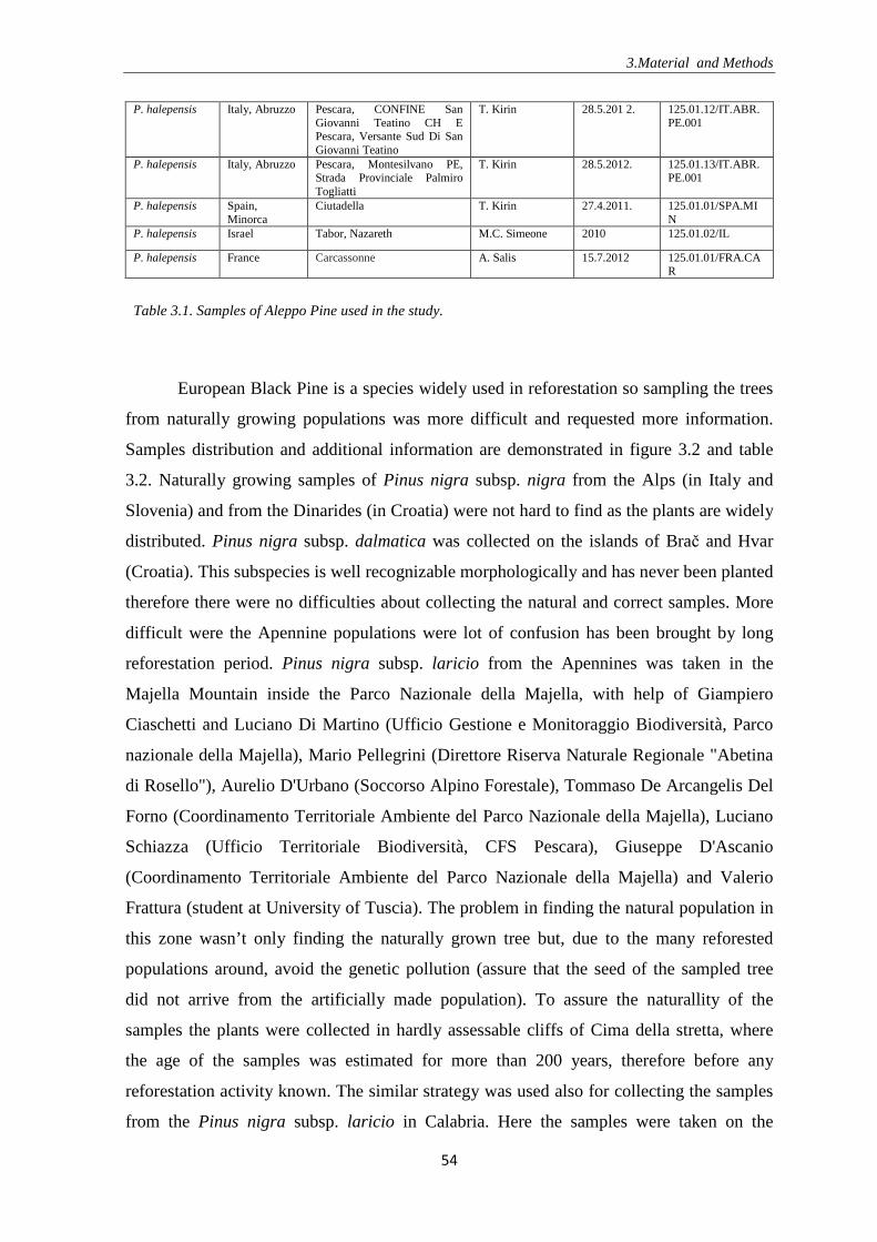
3.Material and Methods
54
P. halepensis Italy, Abruzzo Pescara, CONFINE San Giovanni Teatino CH E Pescara, Versante Sud Di San Giovanni Teatino
T. Kirin 28.5.201 2. 125.01.12/IT.ABR.PE.001
P. halepensis Italy, Abruzzo Pescara, Montesilvano PE, Strada Provinciale Palmiro Togliatti
T. Kirin 28.5.2012. 125.01.13/IT.ABR.PE.001
P. halepensis Spain, Minorca
Ciutadella T. Kirin 27.4.2011. 125.01.01/SPA.MIN
P. halepensis Israel Tabor, Nazareth M.C. Simeone 2010 125.01.02/IL
P. halepensis France Carcassonne A. Salis 15.7.2012 125.01.01/FRA.CAR
Table 3.1. Samples of Aleppo Pine used in the study.
European Black Pine is a species widely used in reforestation so sampling the trees
from naturally growing populations was more difficult and requested more information.
Samples distribution and additional information are demonstrated in figure 3.2 and table
3.2. Naturally growing samples of Pinus nigra subsp. nigra from the Alps (in Italy and
Slovenia) and from the Dinarides (in Croatia) were not hard to find as the plants are widely
distributed. Pinus nigra subsp. dalmatica was collected on the islands of Brač and Hvar
(Croatia). This subspecies is well recognizable morphologically and has never been planted
therefore there were no difficulties about collecting the natural and correct samples. More
difficult were the Apennine populations were lot of confusion has been brought by long
reforestation period. Pinus nigra subsp. laricio from the Apennines was taken in the
Majella Mountain inside the Parco Nazionale della Majella, with help of Giampiero
Ciaschetti and Luciano Di Martino (Ufficio Gestione e Monitoraggio Biodiversità, Parco
nazionale della Majella), Mario Pellegrini (Direttore Riserva Naturale Regionale "Abetina
di Rosello"), Aurelio D'Urbano (Soccorso Alpino Forestale), Tommaso De Arcangelis Del
Forno (Coordinamento Territoriale Ambiente del Parco Nazionale della Majella), Luciano
Schiazza (Ufficio Territoriale Biodiversità, CFS Pescara), Giuseppe D'Ascanio
(Coordinamento Territoriale Ambiente del Parco Nazionale della Majella) and Valerio
Frattura (student at University of Tuscia). The problem in finding the natural population in
this zone wasn’t only finding the naturally grown tree but, due to the many reforested
populations around, avoid the genetic pollution (assure that the seed of the sampled tree
did not arrive from the artificially made population). To assure the naturallity of the
samples the plants were collected in hardly assessable cliffs of Cima della stretta, where
the age of the samples was estimated for more than 200 years, therefore before any
reforestation activity known. The similar strategy was used also for collecting the samples
from the Pinus nigra subsp. laricio in Calabria. Here the samples were taken on the
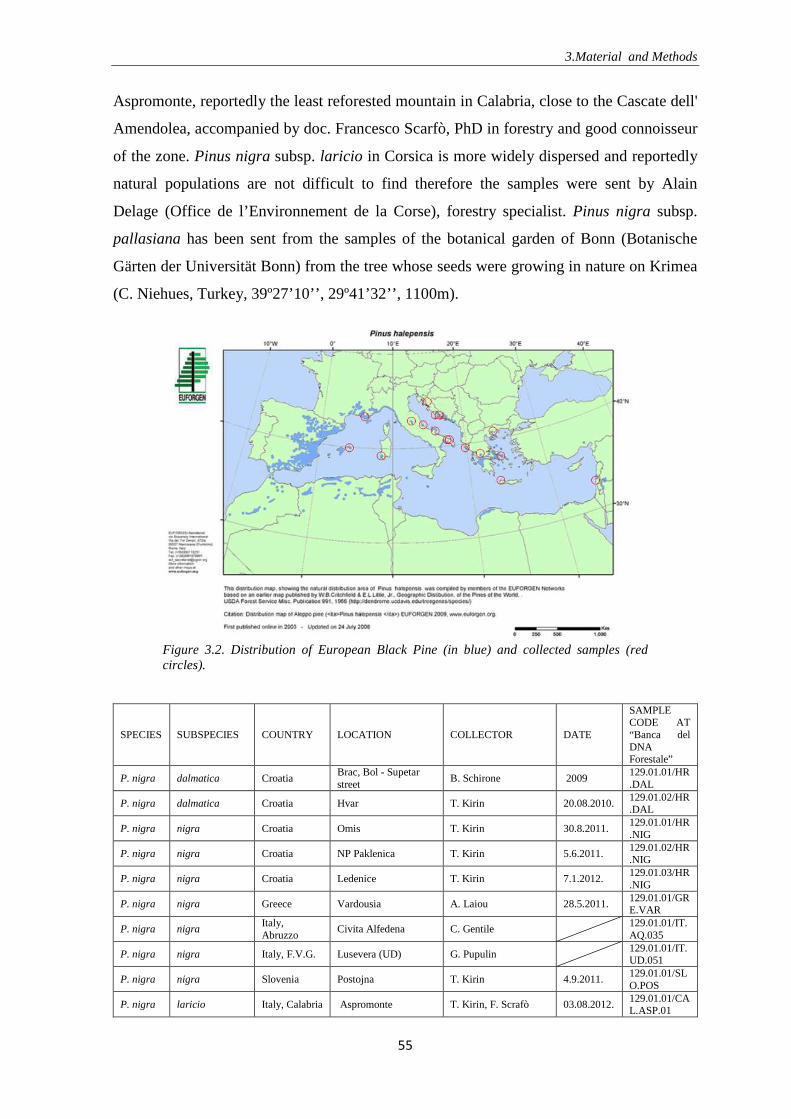
3.Material and Methods
55
Aspromonte, reportedly the least reforested mountain in Calabria, close to the Cascate dell'
Amendolea, accompanied by doc. Francesco Scarfò, PhD in forestry and good connoisseur
of the zone. Pinus nigra subsp. laricio in Corsica is more widely dispersed and reportedly
natural populations are not difficult to find therefore the samples were sent by Alain
Delage (Office de l’Environnement de la Corse), forestry specialist. Pinus nigra subsp.
pallasiana has been sent from the samples of the botanical garden of Bonn (Botanische
Gärten der Universität Bonn) from the tree whose seeds were growing in nature on Krimea
(C. Niehues, Turkey, 39º27’10’’, 29º41’32’’, 1100m).
Figure 3.2. Distribution of European Black Pine (in blue) and collected samples (red circles).
SPECIES SUBSPECIES COUNTRY LOCATION COLLECTOR DATE
SAMPLE CODE AT “Banca del DNA Forestale”
P. nigra dalmatica Croatia Brac, Bol - Supetar street
B. Schirone 2009 129.01.01/HR.DAL
P. nigra dalmatica Croatia Hvar T. Kirin 20.08.2010. 129.01.02/HR.DAL
P. nigra nigra Croatia Omis T. Kirin 30.8.2011. 129.01.01/HR.NIG
P. nigra nigra Croatia NP Paklenica T. Kirin 5.6.2011. 129.01.02/HR.NIG
P. nigra nigra Croatia Ledenice T. Kirin 7.1.2012. 129.01.03/HR.NIG
P. nigra nigra Greece Vardousia A. Laiou 28.5.2011. 129.01.01/GRE.VAR
P. nigra nigra Italy, Abruzzo
Civita Alfedena C. Gentile
129.01.01/IT.AQ.035
P. nigra nigra Italy, F.V.G. Lusevera (UD) G. Pupulin
129.01.01/IT.UD.051
P. nigra nigra Slovenia Postojna T. Kirin 4.9.2011. 129.01.01/SLO.POS
P. nigra laricio Italy, Calabria Aspromonte T. Kirin, F. Scrafò 03.08.2012. 129.01.01/CAL.ASP.01
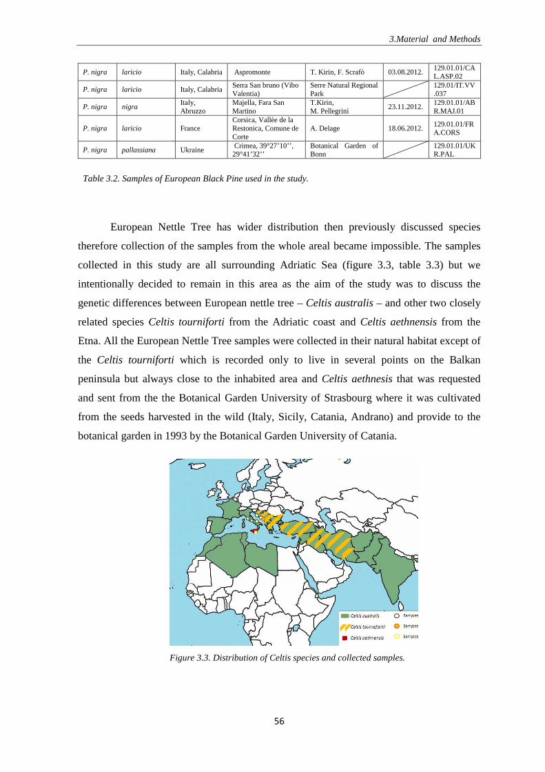
3.Material and Methods
56
P. nigra laricio Italy, Calabria Aspromonte T. Kirin, F. Scrafò 03.08.2012. 129.01.01/CAL.ASP.02
P. nigra laricio Italy, Calabria Serra San bruno (Vibo Valentia)
Serre Natural Regional Park
129.01/IT.VV.037
P. nigra nigra Italy, Abruzzo
Majella, Fara San Martino
T.Kirin, M. Pellegrini
23.11.2012. 129.01.01/ABR.MAJ.01
P. nigra laricio France Corsica, Vallèe de la Restonica, Comune de Corte
A. Delage 18.06.2012. 129.01.01/FRA.CORS
P. nigra pallassiana Ukraine Crimea, 39°27’10’’, 29°41’32’’
Botanical Garden of Bonn
129.01.01/UKR.PAL
Table 3.2. Samples of European Black Pine used in the study.
European Nettle Tree has wider distribution then previously discussed species
therefore collection of the samples from the whole areal became impossible. The samples
collected in this study are all surrounding Adriatic Sea (figure 3.3, table 3.3) but we
intentionally decided to remain in this area as the aim of the study was to discuss the
genetic differences between European nettle tree – Celtis australis – and other two closely
related species Celtis tourniforti from the Adriatic coast and Celtis aethnensis from the
Etna. All the European Nettle Tree samples were collected in their natural habitat except of
the Celtis tourniforti which is recorded only to live in several points on the Balkan
peninsula but always close to the inhabited area and Celtis aethnesis that was requested
and sent from the the Botanical Garden University of Strasbourg where it was cultivated
from the seeds harvested in the wild (Italy, Sicily, Catania, Andrano) and provide to the
botanical garden in 1993 by the Botanical Garden University of Catania.
Figure 3.3. Distribution of Celtis species and collected samples.

3.Material and Methods
57
SPECIES COUNTRY LOCATION COLLECTOR DATE
SAMPLE
CODE AT
“Banca del
DNA
Forestale”
Celtis australis Croatia Omiš T. Kirin 30.8.2011. 373.01.01/HR
Celtis australis Croatia NP Paklenica T. Kirin 5.6.2011. 373.01.02/HR
Celtis australis Italy Abruzzo - San Donato, Val di
Comino T. Kirin 17.4.2011.
373.01.01/IT.
ABR
Celtis australis Italy Apulia - Manfredonia T. Kirin 9.8.2011. 373.01.02/IT.
APU
Celtis aethnensis Italy Sicily - Etna
Bot.Gar.
University of
Strasbourg
373.01.03/IT.S
IC
Celtis tournifortii Croatia Omiš T. Kirin 30.8.2011. 373.02.01/HR
Table 3.3. Samples of genus Celtis used in the study.
Samples of Inula verbascifolia subsp. verbascifolia were collected in Croatia, Italy
and Greece. In Croatia ten samples from three different populations were taken, In Italy
three samples from one (unique) population and in Greece just one sample was taken. One
sample of Inula verbascifolia subsp. parnassica from Greece was taken as an out-group
(figure 3.4, table 3.4).
Figure 3.4. Natural distribution of I. verbascifolia subsp. verbascifolia and the sampling
strategy.
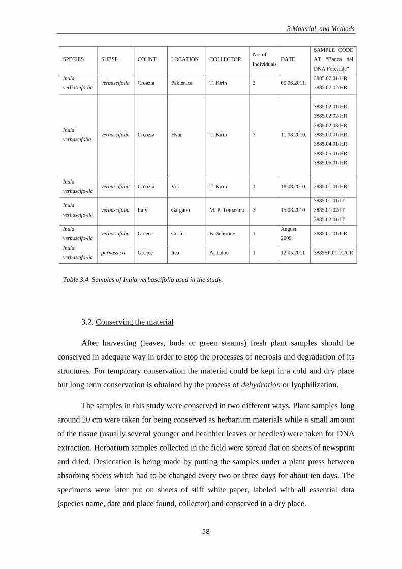
3.Material and Methods
58
SPECIES SUBSP. COUNT.. LOCATION COLLECTOR No. of
individuals DATE
SAMPLE CODE
AT “Banca del
DNA Forestale”
Inula
verbascifo-lia verbascifolia Croazia Paklenica T. Kirin 2 05.06.2011.
3885.07.01/HR
3885.07.02/HR
Inula
verbascifolia verbascifolia Croazia Hvar T. Kirin 7 11.08.2010.
3885.02.01/HR
3885.02.02/HR
3885.02.03/HR
3885.03.01/HR
3885.04.01/HR
3885.05.01/HR
3885.06.01/HR
Inula
verbascifo-lia verbascifolia Croazia Vis T. Kirin 1 18.08.2010. 3885.01.01/HR
Inula
verbascifo-lia verbascifolia Italy Gargano M. P. Tomasino 3 15.08.2010
3885.01.01/IT
3885.01.02/IT
3885.02.01/IT
Inula
verbascifo-lia verbascifolia Greece Corfu B. Schirone 1
August
2009 3885.01.01/GR
Inula
verbascifo-lia parnassica Grecee Itea A. Laiou 1 12.05.2011 3885SP.01.01/GR
Table 3.4. Samples of Inula verbascifolia used in the study.
3.2. Conserving the material
After harvesting (leaves, buds or green steams) fresh plant samples should be
conserved in adequate way in order to stop the processes of necrosis and degradation of its
structures. For temporary conservation the material could be kept in a cold and dry place
but long term conservation is obtained by the process of dehydration or lyophilization.
The samples in this study were conserved in two different ways. Plant samples long
around 20 cm were taken for being conserved as herbarium materials while a small amount
of the tissue (usually several younger and healthier leaves or needles) were taken for DNA
extraction. Herbarium samples collected in the field were spread flat on sheets of newsprint
and dried. Desiccation is being made by putting the samples under a plant press between
absorbing sheets which had to be changed every two or three days for about ten days. The
specimens were later put on sheets of stiff white paper, labeled with all essential data
(species name, date and place found, collector) and conserved in a dry place.
3.Material and Methods
59
The material predestined for a DNA extraction was conserved in the silica gel
already in the field. This is the most commonly used and the most efficient method of
dehydration of the plants especially for the fact that it is easily brought in the field and
therefore the dehydration of the tissue starts the moment sample is collected. Dehydrated
silica-gel in being put in a ziplock style, plastic bag and brought on the field. Collected
material is put in a bag and closed. After several days the sample is dry and ready for the
DNA extraction. The used silica gel can be reused after dehydrating it in the oven by
heating it to 120°C for two hours. All the samples, herbarium and lyophilized ones, were
conserved in the Banca del DNA Forestale at the University of Tuscia.
3.3 DNA extraction
Lyophilized material was grinded to a powder with a mortar and pestle in the presence
of a pinch of silica (silicon dioxide, SiO2). The finer the grind is the greater will be the
yield of DNA from a given amount of material, so the process needs to be done patiently.
The process of extractions starts from the 20 mg of the plant tissue and is being derived
with DNAeasy Plant Mini Kit (Quiagen). The extraction fazes are following six:
1. Cell lysis and RNA elimination
PROCEDURE:
a. Put Buffer AP1 (Lysis buffer, 40 ml) in bain-marie (water bath) at 65˚C.
b. Take out RNase A (220�l) from the freezer
c. Prepare tubes (not supplied), write numbers/names on them
d. Put samples in tubes (around 30 mg)
e. Add few milligrams (2-3) of PVPP (polyvinyl polypyrrolidone, used for removing
polyphenols)
f. Add 600 �l of warmed Buffer AP1 (Lysis buffer, 40 ml)
g. Add 4 �l of RNase (used to avoid the RNA contamination of the sample)
h. Vortex
i. Put in bain-marie for 30 minutes, each 10 minutes vortex
2. Precipitation of the detergent, proteins, and polysaccharides

3.Material and Methods
60
PROCEDURE:
a. Add 200 �l of Buffer AP2 (Precipitation buffer, 18 ml)
b. Vortex
c. Put in freezer for 5 minutes
d. Centrifuge for 5 minutes at max (14 800 r.p.m.)
3. Filtration of the residual cell tissues
PROCEDURE:
a. Pipet hole liquid part from the old tubes into the pink ones. Add also a little of solid
part.
b. Centrifuge for 2 minutes at max (14 800 r.p.m.)
4. Binding of the DNA to a molecular exchange column
PROCEDURE:
a. Throw away the small tubes inside of the big ones.
b. Transfer liquid part from the pink tubes to the new ones (without the caps) - Do
not touch the solid part formed on the bottom
c. Add the quantity 1.5 of volume of Buffer AP3/E (Binding buffer, 30�l
concentrate; before use check if ethanol has been added!). e.g.: 500 �l of sample
�750 �l of AP3/E, 600 �l of sample �900 �l of AP3/E, 750 �l of sample
�1125 �l of AP3/E
d. Mix by pipetting 10 times, and leave the tips inside of the tubes
e. Transfer 680 �l of sample in new white tubes
f. Centrifuge for 1 minute at 10 000 r.p.m.
g. Throw the flow-through
h. Transfer the remaining sample in white tubes
i. Centrifuge for 1 minute at 10 000 rpm
j. Throw the flow-through
5. Washing the DNA

3.Material and Methods
61
PROCEDURE:
a. Transfer little tubes in big ones in the Kit (Collection Tubes, 2 ml)
b. Add 500 �l of Buffer AW (Wash buffer, 17 ml concentrate; before use check if
ethanol has been added!)
c. Centrifuge for 1 minute at 8 000 r.p.m.
d. Throw the flow-through
e. Add 500 �l of Buffer AW (Wash buffer, 17 ml concentrate; before use check if
ethanol has been added!)
f. Centrifuge for 2 minutes at max (14 800 r.p.m.)
6. Eluting the DNA
PROCEDURE:
a. Transfer little tubes in new big ones (not supplied), cut the caps
b. Add 75 �l of Buffer AE (Elution buffer, 12 ml) directly on the DNeasy
membrane
c. Incubate for 5 minutes at room temperature
d. Centrifuge for 1 minute at 10 000 r.p.m.
e. Add 75 �l of Buffer AE (Elution buffer, 12 ml) directly on the DNeasy
membrane
f. Incubate for 5 minutes at room temperature
g. Centrifuge for 1 minute at 10 000 r.p.m.
h. Throw the little tubes
i. Put caps with numbers/names on the tubes
j. Centrifuge for 1o seconds at max (14 800 r.p.m.)
k. Put at -20°C to conserve
3.Material and Methods
62
3.4. Amplification of the fragment using the PCR machine
The polymerase chain reaction (PCR) is a biochemical technology used to amplify
a single or a few copies of a part (selected region) of DNA, generating thousands to
millions of copies of a particular DNA sequence.
A basic PCR requires following components and reagents:
• DNA template that contains the DNA region (target) to be amplified.
• Two complementary primers, which start and finish the amplified region.
• Taq polymerase, thermostable enzyme that synthesizes DNA molecules
from their nucleotide building blocks.
• Deoxynucleoside triphosphates (dNTPs; nucleotides containing triphosphate
groups), the building-blocks from which the DNA polymerase synthesizes a
new DNA strand.
• Buffer solution, providing a suitable chemical environment for optimum
activity and stability of the DNA polymerase.
• Divalent cations, magnesium or manganese ions; generally Mg2+ is used, but
Mn2+ can be utilized for PCR-mediated DNA mutagenesis, as higher Mn2+
concentration increases the error rate during DNA synthesis.
• Monovalent cation potassium ions.
In order to uniform the procedure, in this study PuReTaq Ready-to-go PCR beads
(Amersham) were used which represent the already prepared mixture of dNTPs,
polymerase, buffer and ions ready to put inside the sample and use.
PROCEDURE (PREPARATION OF THE SAMPLE):
In the PCR tubes mix:
1. Extra pure water (Milli-Q water), if needed to arrive at quantity of 5�l mixture of water and DNA
2. DNA
Make mix [2,5 �l (primer f) *X (number of samples) + 2,5 �l (primer r) * X (number of samples) + 15 �l (H20)* X (number of samples)] in another tube
3. 20 �l of the mix 4. PuReTaq Ready-to-go PCR beads
Centrifuge for few seconds
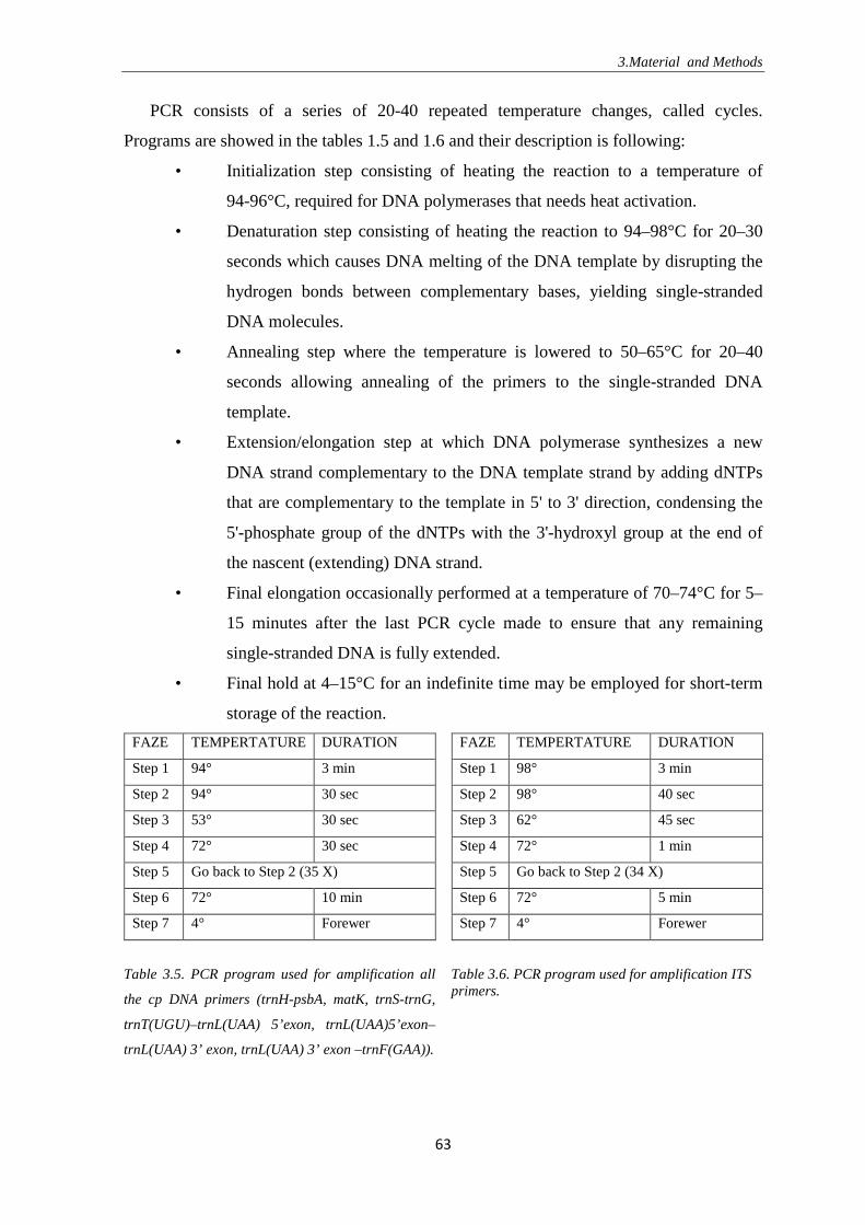
3.Material and Methods
63
PCR consists of a series of 20-40 repeated temperature changes, called cycles.
Programs are showed in the tables 1.5 and 1.6 and their description is following:
• Initialization step consisting of heating the reaction to a temperature of
94-96°C, required for DNA polymerases that needs heat activation.
• Denaturation step consisting of heating the reaction to 94–98°C for 20–30
seconds which causes DNA melting of the DNA template by disrupting the
hydrogen bonds between complementary bases, yielding single-stranded
DNA molecules.
• Annealing step where the temperature is lowered to 50–65°C for 20–40
seconds allowing annealing of the primers to the single-stranded DNA
template.
• Extension/elongation step at which DNA polymerase synthesizes a new
DNA strand complementary to the DNA template strand by adding dNTPs
that are complementary to the template in 5' to 3' direction, condensing the
5'-phosphate group of the dNTPs with the 3'-hydroxyl group at the end of
the nascent (extending) DNA strand.
• Final elongation occasionally performed at a temperature of 70–74°C for 5–
15 minutes after the last PCR cycle made to ensure that any remaining
single-stranded DNA is fully extended.
• Final hold at 4–15°C for an indefinite time may be employed for short-term
storage of the reaction.
FAZE TEMPERTATURE DURATION
Step 1 94° 3 min
Step 2 94° 30 sec
Step 3 53° 30 sec
Step 4 72° 30 sec
Step 5 Go back to Step 2 (35 X)
Step 6 72° 10 min
Step 7 4° Forewer
FAZE TEMPERTATURE DURATION
Step 1 98° 3 min
Step 2 98° 40 sec
Step 3 62° 45 sec
Step 4 72° 1 min
Step 5 Go back to Step 2 (34 X)
Step 6 72° 5 min
Step 7 4° Forewer
Table 3.5. PCR program used for amplification all
the cp DNA primers (trnH-psbA, matK, trnS-trnG,
trnT(UGU)–trnL(UAA) 5’exon, trnL(UAA)5’exon–
trnL(UAA) 3’ exon, trnL(UAA) 3’ exon –trnF(GAA)).
Table 3.6. PCR program used for amplification ITS primers.
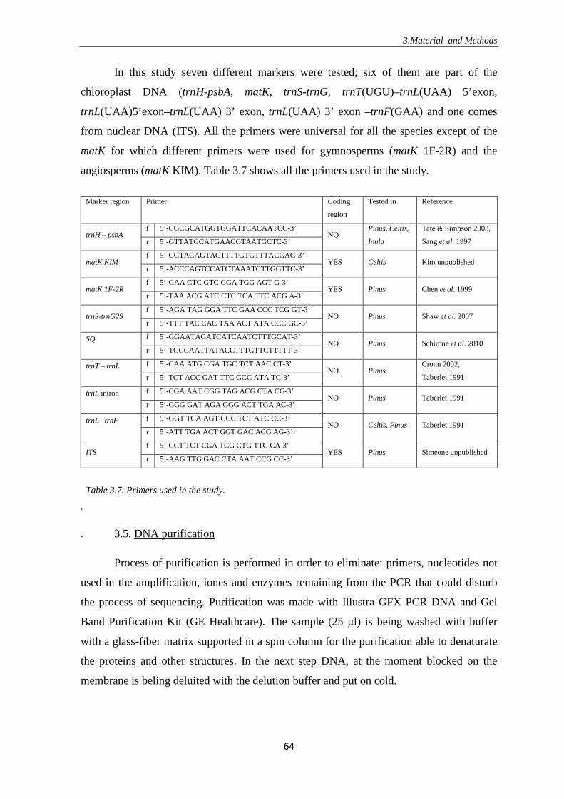
3.Material and Methods
64
In this study seven different markers were tested; six of them are part of the
chloroplast DNA (trnH-psbA, matK, trnS-trnG, trnT(UGU)–trnL(UAA) 5’exon,
trnL(UAA)5’exon–trnL(UAA) 3’ exon, trnL(UAA) 3’ exon –trnF(GAA) and one comes
from nuclear DNA (ITS). All the primers were universal for all the species except of the
matK for which different primers were used for gymnosperms (matK 1F-2R) and the
angiosperms (matK KIM). Table 3.7 shows all the primers used in the study.
Marker region Primer Coding
region
Tested in Reference
trnH – psbA f 5’-CGCGCATGGTGGATTCACAATCC-3’
NO Pinus, Celtis,
Inula
Tate & Simpson 2003,
Sang et al. 1997 r 5’-GTTATGCATGAACGTAATGCTC-3’
matK KIM f 5’-CGTACAGTACTTTTGTGTTTACGAG-3’
YES Celtis Kim unpublished r 5’-ACCCAGTCCATCTAAATCTTGGTTC-3’
matK 1F-2R f 5’-GAA CTC GTC GGA TGG AGT G-3’
YES Pinus Chen et al. 1999 r 5’-TAA ACG ATC CTC TCA TTC ACG A-3’
trnS-trnG2S f 5’-AGA TAG GGA TTC GAA CCC TCG GT-3’
NO Pinus Shaw et al. 2007 r 5’-TTT TAC CAC TAA ACT ATA CCC GC-3’
SQ f 5’-GGAATAGATCATCAATCTTTGCAT-3’ NO Pinus Schirone et al. 2010
r 5’-TGCCAATTATACCTTTGTTCTTTTT-3’
trnT – trnL f 5’-CAA ATG CGA TGC TCT AAC CT-3’ NO Pinus
Cronn 2002,
Taberlet 1991 r 5’-TCT ACC GAT TTC GCC ATA TC-3’
trnL intron f 5’-CGA AAT CGG TAG ACG CTA CG-3’ NO Pinus Taberlet 1991
r 5’-GGG GAT AGA GGG ACT TGA AC-3’
trnL –trnF f 5’-GGT TCA AGT CCC TCT ATC CC-3’ NO Celtis, Pinus Taberlet 1991
r 5’-ATT TGA ACT GGT GAC ACG AG-3’
ITS f 5’-CCT TCT CGA TCG CTG TTC CA-3’
YES Pinus Simeone unpublished r 5’-AAG TTG GAC CTA AAT CCG CC-3’
Table 3.7. Primers used in the study.
.
. 3.5. DNA purification
Process of purification is performed in order to eliminate: primers, nucleotides not
used in the amplification, iones and enzymes remaining from the PCR that could disturb
the process of sequencing. Purification was made with Illustra GFX PCR DNA and Gel
Band Purification Kit (GE Healthcare). The sample (25 µl) is being washed with buffer
with a glass-fiber matrix supported in a spin column for the purification able to denaturate
the proteins and other structures. In the next step DNA, at the moment blocked on the
membrane is beling deluited with the delution buffer and put on cold.
3.Material and Methods
65
PROCEDURE:
1. Put numbers on tubes (Collection tubes, 50 pack), cut the caps and insert little tubes
inside (illustra GFX MicroSpin columns, 50 pack)
2. Add 500 �l of Buffer (Capture Buffer Type 3, BLUE CAP)
3. Add hole DNA made by PCR (~30 �l)
4. Mix by pipetting 10 times
5. Centrifuge for 35 seconds at max (14 800 r.p.m.)
6. Throw the flow-through in the big black jar for liquid waste
7. Add 500 �l of Buffer (Capture Buffer Type 1, YELLOW CAP, 25 ml; before use
check if ethanol has been added!)
8. Centrifuge for 35 seconds at max (14 800 rpm)
9. Add 500 �l of Buffer (Capture Buffer Type 1, YELLOW CAP)
10. Centrifuge for 35 seconds at max (14 800 r.p.m.)
11. Centrifuge for 2 minutes at max (14 800 r.p.m.)
12. Put numbers on new tubes (not supplied) and cut the caps
13. Throw the old big tubes and the small ones put in the new big ones
14. Add 30 �l of Buffer (Elution buffer type 6, PINK CAP)
15. Incubate for 2 minutes
16. Centrifuge for 1 minute at max (14 800 r.p.m.)
17. Throw the small tubes and put the caps on the big ones
18. Keep them in at -20°C if they need to wait
3.6. DNA fragments verification – Gel electrophoresis
Gel electrophoresis is a method for separation and analysis of macromolecules
(DNA, RNA and proteins) and their fragments, based on their size and charge. In this study
it was used three times; in order to verify the precense and the quantity of the DNA after
the DNA extraction, after PCR to confirm the length of the sequences obtained, after
purification in order to confirm the preveously observed result.
Electrophoresis is performed using an electric field under which molecules (such as
DNA) can move through a gel made of agar. The molecules being sorted are dispensed into
a well of in the gel material. The gel is placed in an electrophoresis chamber filled with
3.Material and Methods
66
buffer (usually Tris/Borate/EDTA (TBE)), which is then connected to a power source.
When the electric current is applied, the larger molecules move more slowly through the
gel while the smaller molecules move faster. The different sized molecules form distinct
bands on the gel.
After the electrophoresis is complete, the molecules in the gel can be stained to
make them visible. DNA was at the begining visualized using ethidium bromide which,
when intercalated into DNA, fluoresce under ultraviolet light.
Bromophenol blue are common dyes found in loading buffers; they run about the
same speed as DNA fragments that are 5000 bp and 300 bp in length respectively, but the
precise position varies with percentage of the gel.
After electrophoresis the gel is illuminated with an ultraviolet lamp (usually by
placing it on a light box, while using protective gear to limit exposure to ultraviolet
radiation). The illuminator apparatus mostly also contains imaging apparatus that takes an
image of the gel, after illumination with UV radiation.
3.7. DNA sequencing
Purificated sequences have initially been sent on sequencing in the laboratory of
Eurofins MWG Operon and later, due to the lower cost of sequencing, to the laboratory of
Macrogen Inc. (Europe). Both laboratories use the same methods with similar type of
sequencer therefore the quality of results was the same. Sequencing method was always the
same, most commonly used, Sanger sequencing, already explained in the introduction. The
results are depicted in the form of a chromatogram, which is a diagram of coloured peaks
that correspond to the nucleotide in that location in the sequence.
3.8. Bioinformatics
3.8.1. Chromatogram visualization
Chromatogram (sometimes also called electropherogram) which arrives as a result
of the sequencing is produced by a sequencing machine and could be of different quality.
3.Material and Methods
67
Sometimes it can contain some reading errors due to the algorithm used for reading it. The
errors are especially often at the beginning and, sometimes, also at the end of the sequence
so these are the parts that need to be corrected particularly cautiously. Some markers are
more characteristic for producing low quality chromatograms usually due to their poly-
repeating regions. Visual correction of the chromatogram is the first step that needs to be
made in a process of sequences operating. The programs used for visualizing the
chromatograms are Chromas, BioEdit, DNAMann. In this study BioEdit (Hall 1999) was
used for visualization as it has a clear and simple interface. Another attractive
characteristic of the program is the configuration which automatically saves the edited
sequence in a new file which guaranties the conservation of the original chromatogram.
3.8.2. Multiple sequence alignment
As already mentioned in the introduction multiple alignment is very sensitive and
important part of any genetic analysis. In this study the alignments were made in the
Seaview 4.2. (Galtier et al. 1996) program which uses the MUSCLE (Multi-Alignment
Fast Fourier Trasformation) algorithm (Edgar 2004) with its standard settings. In this case
sequences were not very variable and the number of sequences was relatively small so
alignment was performed almost instantly in Seaview 4.2.. More complex multiple
alignment can take lot of time and require more hardware resources then normally
available on a personal computer so it is advisable to obtain the alignment using an online
service. One of such services (also using the MAFFT standard algorithm) is
“Bioinformatics toolkit” managed by Max-Planck Institute
(http://toolkit.tuebingen.mpg.de/mafft).
3.8.3. Mesquite 2.75
Mesquite (Madison & Madison 2011) is software designed to help perform
phylogenetic analysis. Since it is modular, the analyses available depend on the modules
installed. Analyses include: reconstruction of ancestral states (parsimony, likelihood); tests
of process of character evolution, including correlation; analysis of speciation and
extinction rates; simulation of character evolution (categorical, DNA, continuous);
parametric bootstrapping; morphometrics; coalescence; tree comparisons and simulations.
In this study it was sometimes used for observing multiple alignment, to extraction of the
variable sites and parsimony informative sites and for visualization of the phylogenetic
trees obtained with other programs.

3.Material and Methods
68
3.8.4. DnaSP 5.10
DnaSP, DNA Sequence Polymorphism, is a software package for the analysis of
nucleotide polymorphism from the aligned DNA sequence data (Librado & Rozas 2009).
DnaSP can estimate several measures of DNA sequence variation within and between
populations (in noncoding, synonymous or nonsynonymous sites, or in various sorts of
codon positions), as well as linkage disequilibrium, recombination, gene flow and gene
conversion parameters. DnaSP can also carry out several tests of neutrality and can
estimate the confidence intervals of some test-statistics by the coalescent. The results of the
analyses are displayed on tabular and graphic form. In this study DnaSP software was used
to calculate the In/Del, variable, polymorphic and parsimony sites. Furthermore the
program was used for visualization of haplotypes and for calculating the haplotype
diversity.
3.8.5. Mega 5.0.
MEGA is an integrated tool for conducting sequence alignment, inferring
phylogenetic trees, mining web-based databases, estimating rates of molecular evolution,
inferring ancestral sequences, and testing evolutionary hypotheses. The objective of the
MEGA software is to provide tools for exploring, discovering, and analyzing DNA and
protein sequences from an evolutionary perspective. MEGA software obtains phylogenetic
trees from molecular data with Distance methods, Parsimony methods, and Likelihood
methods. In this study MEGA was used to perform the distance matrix phylogeny with
Neighbor-Joining method which can be made changing several settings and evolutionary
models. In order to choose the best model I decided to use jModelTest2 (Posada 2003), a
tool which carries out statistical selection of best-fit models of nucleotide substitution.
Model selection strategy inside the jModelTest2 used was Akaike information criteria
(AIC), which would calculate the most recommended model. Model suggested in
jModelTest I would choose when setting up the phylogenetic tree in MEGA. The
evolutionary models used in this study were different and are mentioned under each
phylogenetic tree in the results. Other settings I used when programming the phylogenetic
tree were the same for each analysis (No. of bootstrap replications was 1000; substitutions
included transitions and transversions; rates among sites were uniform; patterns among
lineages were homogeneous; for Gaps/Missing data I used the option called the Complete-
Deletion meaning that such places were eliminated from the analyses). Even though my

3.Material and Methods
69
dataset was destitute with variable sites so Complete-Deletion function caused even less
informative trees I decided to use it as it is the most recommended approach in distance
matrix phylogeny and since it was not the only method I used in the study I wasn’t afraid
of totally loosing an important information.
3.8.6. RAxML
For many datasets, a full maximum likelihood analysis is extremely
computationally expensive. Software packages developed to conduct rapid maximum
likelihood analyses are GARLI, IQPNNI, PHYML, and RAxML. In this study I used
RAxML (Randomized Axelerated Maximum Likelihood) software which was developed
by Alexandros Stamatakis (Stamatakis 2006). The command line used to obtain the
analyses was:
raxmlHPC –f a –x 12345 -p 1234 -# 1000 –q “partitition file name” -s “name file input” –
m GTRGAMMA -n “name file output”
in which:
-x 12345 denotes a random number permitting the use of bootstrap algorithm
-p 12345 denotes an internal random number to perform the parsimony inferences
-# denotes a number of the runs in which the software calculates ML (Maximum
Likelihood) using–f and –x to call a fast bootstrap and ML analysis of the
alignment
-s denotes an input file (necessary in PHYLIP format, but important not to write the
extension behind the file name)
-m denotes sequences substitution model used to estimate ML. In this study the
model used was GTR+Γ
-n denotes the output file
After finishing the analysis the consensus tree is found in a file called
„RaxMl_bipartitions” and it was viewed in a graphical viewer of phylogenetic trees
FigTree (http://tree.bio.ed.ac.uk/software/figtree/) ,.
3.Material and Methods
70
3.8.7. MrBayes
MrBayes 3.2 (Ronquist et al. 2011) is a program for Bayesian inference and model
choice across a wide range of phylogenetic and evolutionary models. MrBayes uses
Markov chain Monte Carlo (MCMC) methods to estimate the posterior distribution of
model parameters. This program offers particularly large spectrum of settings from which
only the ones changed from the default are reported.
First the information about the partitition was inserted in order to separate each
marker from another. As the sequences from all the partititions originated from the
chloroplast DNA with generally same characteristics all the settings were kept equal for all
the partititions.
Basic model settings offered by the program are following:
• Nucmodel – offers to choose the general type of DNA model; 4by4, standard
nucleotide substitution model was chosen in this study
• Nst – representing the structure of the substitution model was changed from
standard 1 (JC model) to 6 (GTR model)
• Code – was set to be Universal as it is a setting important only when dealing with a
Codon model
• Ploidy – was changed from diploid to haploid as al the sequences were made from
cpDNA
• Rates – were changed from Equal (no rate variation across sites) to Invgamma
(gamma-shaped rate variation with a proportion of invariable sites).
• Ngammacat – denoting the number of discrete categories used to approximate the
gamma distribution, was left 4 as a default
• Usegibbs (No), Gibbsfreq (100), Nbetacat (5), Omegavar (Equal), Coding (All) –
are all the settings advised to leave since default as they are used only in some
specific cases not for single nucleotide models
• Covarion (No), Parsmodel (No) – denotes the specific calculation models
(covarion and parsimony) that could be used; in this study were not used
The priors set were left as it is default (figure 3.5).

3.Material and Methods
71
Figure 3.5. Priors configuration settings.
Run settings, on the other hand, were slightly adjusted to proper study (figure 3.6).

3.Material and Methods
72
Figure 3.6. Standard configuration run settings.
From the standard settings the following states were changed:
• Diagnfreq was changed from the default 5000 (more appropriate for a larger
analysis) to 1000 meaning that the diagnostics will be computed more often
• Another setting good to change on a smaller dataset is Samplefreq, stating how
often the chain is sampled. From the default 500 generations it was turned to 100
since in the small datasets it is recommended to sample more often so that the
analysis don’t converge too rapidly.
At the end of the run, program asks whether or not we want to continue with the
analysis. To answer that question it is necessary to examine the average standard deviation
of split frequencies. A rough guide is that an average standard deviation below 0.01 is very
good indication of convergence, while values between 0.01 and 0.05 may be adequate
depending on the purpose of your analysis. Alternative method to test if the values have
converged enough to stop the analysis is to open the output program in the program called
Tracer. This program offers the graphic visualization of the Bayesian runs which can give
us a clearer vision of how close the results got one to each other.
3.8.8. Network 4.6.1.1.
Network is a program which generates evolutionary networks from genetic,
linguistic, and other data. Its input data were previously revised and adjusted in Mesquite
and in Microsoft Excel. The procedure of adjustment consisted of opening the multiple
alignment in the Mesquite, choosing the option to mark the parsimony informative sites
and copying them in the Excel. Inside spreadsheet the selected sites would be eliminated
based on two assumptions (first is that multi-insertions/deletions were evolutionary one
event and the second is the same statement considering inversions). In these cases I used to

3.Material and Methods
73
eliminate all the sites except from the one in order to avoid long branches in the network
which make the impression of numerous evolutionary events while in reality were
presenting one insertion of several bases (however one event). Such adjusted data had to be
transformed, using clean text editor like Notepad, into .fasta configuration, readable by the
Network.
The program offers two types of network construction (using the Median Joining or
Reduced Median algorithm) and directly makes the haplotype network. The networks can
later be adjusted in the same program or can be imported to a graphic programs to obtain
the better presentation of the data obtained.
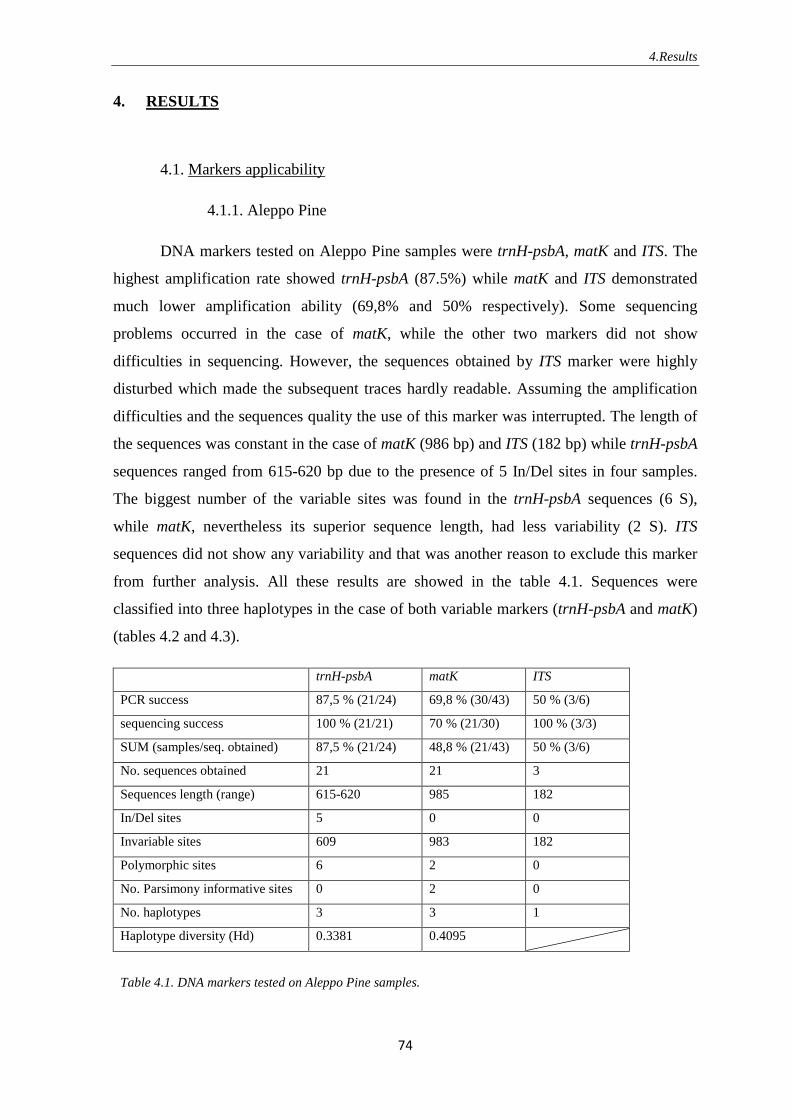
4.Results
74
4. RESULTS
4.1. Markers applicability
4.1.1. Aleppo Pine
DNA markers tested on Aleppo Pine samples were trnH-psbA, matK and ITS. The
highest amplification rate showed trnH-psbA (87.5%) while matK and ITS demonstrated
much lower amplification ability (69,8% and 50% respectively). Some sequencing
problems occurred in the case of matK, while the other two markers did not show
difficulties in sequencing. However, the sequences obtained by ITS marker were highly
disturbed which made the subsequent traces hardly readable. Assuming the amplification
difficulties and the sequences quality the use of this marker was interrupted. The length of
the sequences was constant in the case of matK (986 bp) and ITS (182 bp) while trnH-psbA
sequences ranged from 615-620 bp due to the presence of 5 In/Del sites in four samples.
The biggest number of the variable sites was found in the trnH-psbA sequences (6 S),
while matK, nevertheless its superior sequence length, had less variability (2 S). ITS
sequences did not show any variability and that was another reason to exclude this marker
from further analysis. All these results are showed in the table 4.1. Sequences were
classified into three haplotypes in the case of both variable markers (trnH-psbA and matK)
(tables 4.2 and 4.3).
trnH-psbA matK ITS
PCR success 87,5 % (21/24) 69,8 % (30/43) 50 % (3/6)
sequencing success 100 % (21/21) 70 % (21/30) 100 % (3/3)
SUM (samples/seq. obtained) 87,5 % (21/24) 48,8 % (21/43) 50 % (3/6)
No. sequences obtained 21 21 3
Sequences length (range) 615-620 985 182
In/Del sites 5 0 0
Invariable sites 609 983 182
Polymorphic sites 6 2 0
No. Parsimony informative sites 0 2 0
No. haplotypes 3 3 1
Haplotype diversity (Hd) 0.3381 0.4095
Table 4.1. DNA markers tested on Aleppo Pine samples.
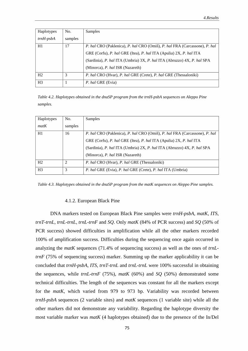
4.Results
75
Haplotypes
trnH-psbA
No.
samples
Samples
H1 17 P. hal CRO (Paklenica), P. hal CRO (Omiš), P. hal FRA (Carcassone), P. hal
GRE (Corfu), P. hal GRE (Itea), P. hal ITA (Apulia) 2X, P. hal ITA
(Sardinia), P. hal ITA (Umbria) 3X, P. hal ITA (Abruzzo) 4X, P. hal SPA
(Minorca), P. hal ISR (Nazareth)
H2 3 P. hal CRO (Hvar), P. hal GRE (Crete), P. hal GRE (Thessaloniki)
H3 1 P. hal GRE (Evia)
Table 4.2. Haplotypes obtained in the dnaSP program from the trnH-psbA sequences on Aleppo Pine
samples.
Haplotypes
matK
No.
samples
Samples
H1 16 P. hal CRO (Paklenica), P. hal CRO (Omiš), P. hal FRA (Carcassone), P. hal
GRE (Corfu), P. hal GRE (Itea), P. hal ITA (Apulia) 2X, P. hal ITA
(Sardinia), P. hal ITA (Umbria) 2X, P. hal ITA (Abruzzo) 4X, P. hal SPA
(Minorca), P. hal ISR (Nazareth)
H2 2 P. hal CRO (Hvar), P. hal GRE (Thessaloniki)
H3 3 P. hal GRE (Evia), P. hal GRE (Crete), P. hal ITA (Umbria)
Table 4.3. Haplotypes obtained in the dnaSP program from the matK sequences on Aleppo Pine samples.
4.1.2. European Black Pine
DNA markers tested on European Black Pine samples were trnH-psbA, matK, ITS,
trnT-trnL, trnL-trnL, trnL-trnF and SQ. Only matK (84% of PCR success) and SQ (50% of
PCR success) showed difficulties in amplification while all the other markers recorded
100% of amplification success. Difficulties during the sequencing once again occurred in
analyzing the matK sequences (71.4% of sequencing success) as well as the ones of trnL-
trnF (75% of sequencing success) marker. Summing up the marker applicability it can be
concluded that trnH-psbA, ITS, trnT-trnL and trnL-trnL were 100% successful in obtaining
the sequences, while trnL-trnF (75%), matK (60%) and SQ (50%) demonstrated some
technical difficulties. The length of the sequences was constant for all the markers except
for the matK, which varied from 979 to 973 bp. Variability was recorded between
trnH-psbA sequences (2 variable sites) and matK sequences (1 variable site) while all the
other markers did not demonstrate any variability. Regarding the haplotype diversity the
most variable marker was matK (4 haplotypes obtained) due to the presence of the In/Del

4.Results
76
site as well as the polymorphic site inside the sequences. Another variable marker was
trnH-psbA and obtained 2 haplotypes. All the other markers did not demonstrate any
variability between the few distant samples and therefore were eliminated from the further
analysis. All the results are shown in the tables 4.4, 4.5 and 4.6.
trnH-psbA matK ITS trnT-trnL trnL-trnL trnL-trnF SQ
PCR success 100 %
(15/15)
84 %
(21/25)
100 %
(3/3)
100 %
(4/4)
100 %
(4/4)
100 %
(4/4)
50%
(3/6)
sequencing
success
100 %
(15/15)
71,4 %
(15/21)
100 %
(3/3)
100 %
(4/4)
100 %
(4/4)
75 % (3/4) 100 %
(3/3)
SUM
(samples/seq.
obtained)
100 %
(15/15)
60 %
(15/25)
100 %
(3/3)
100 %
(4/4)
100 %
(4/4)
75 % (3/4) 50%
(3/6)
No. sequences
obtained
15 15 3 4 4 3 3
Sequences
length (range)
637 973-979 182 461 416 505 486
In/Del sites 0 6 0 0 0 0 0
Invariable sites 635 972 182 461 416 505 486
Polymorphic
sites
2 1 0 0 0 0 0
No. Parsimony
informative sites
0 1 0 0 0 0 0
No. haplotypes 2 4 1 1 1 1 1
Haplotype
diversity (Hd)
0,1333 0.4667
Table 4.4. DNA markers tested on European Black Pine samples.
Haplotypes
trnH-psbA
No. samples Samples
H1 14 P. nig CRO (Brač), P. nig CRO (Hvar), P. nig CRO (Omiš), P. nig CRO
(Ledenice), P. nig FRA (Corsica), P. nig GRE (Vardousia), P. nig ITA
(Calabria-PN Serre), P. nig ITA (FVG), P. nig SLO (Postojna), P. nig
UKR (Crimea), P. nig ITA (Calabria-Aspromonte) 2X, P. nig ITA
(Abruzzo-C. Alfedena), P. nig CRO (Paklenica)
H2 1 P. nig ITA (Majella)
Table 4.5. Haplotypes obtained in the dnaSP program from the trnH-psbA sequences on European Black
Pine.

4.Results
77
Haplotypes
matK
No.
samples
Samples
H1 1 P. nig ITA (Calabria-Aspromonte)
H2 1 P. nig ITA (Calabria-Aspromonte)
H3 11 P. nig CRO (Brač), P. nig CRO (Hvar), P. nig CRO (Omiš), P. nig CRO
(Ledenice), P. nig FRA (Corsica), P. nig GRE (Vardousia), P. nig ITA
(Calabria – PN Serre), P. nig ITA (FVG), P. nig ITA (Majella), P. nig SLO
(Postojna), P. nig UKR (Crimea)
H4 2 P. nig ITA (Abruzzo – C. Alfedena), P. nig CRO (Paklenica)
Table 4.6. Haplotypes obtained in the dnaSP program from the matK sequences on European Black Pine.
4.1.3. European Nettle Tree
DNA markers tested on European Nettle Tree samples were trnH-psbA, matK,
trnS-trnG2S, trnT-trnL and trnL-trnF. Amplification of the marker turned out to be the first
complication in analyzing these samples. The only marker demonstrating the easy
amplification was trnL-trnF (100% of amplification and sequencing success), while
trnH-psbA and matK were much less successful (both managed to obtain 54.5% of the
samples due to amplification and sequencing difficulties). TrnS-trnG2S marker was
amplified in 60% of the samples and 33% of these were successfully sequenced. As a
result only one sequence was obtained; not enough neither to test its variability. However,
the marker was expeld from further analyses. Amplification of trnT-trnL was tested on four
samples but since none of the temptations was successful (two were tried on 54° and two
on 50°C) it was eliminated from the further analysis. Sequences obtained by matK and
trnL-trnF were constant in their length (835 bp and 326 bp, respectively) while the ones
obtained by trnH-psbA ranged from 394 to 399 bp. Polymorphic sites were present in the
sequences of matK while trnH-psbA and trnL-trnF sequences have no variability in the
nucleotide bases (table 4.7). Both trnH-psbA and matK managed to obtain 2 haplotypes
while the trnL-trnF sequences turned out to be totally identical (tables 4.8 and 4.9).
trnH-psbA matK trnS-trnG2S trnT-trnL trnL-trnF
PCR success 54.5 % (6/11) 63.6 % (7/11) 60 % (3/5) 0/4 100 % (6/6)
Sequencing success 100 % (6/6) 85.7 % (6/7) 33% (1/3) 100 % (6/6)
SUM (samples/seq.
obtained)
54.5 % (6/11) 54.5 % (6/11) 20 % (1/5) 100 % (6/6)
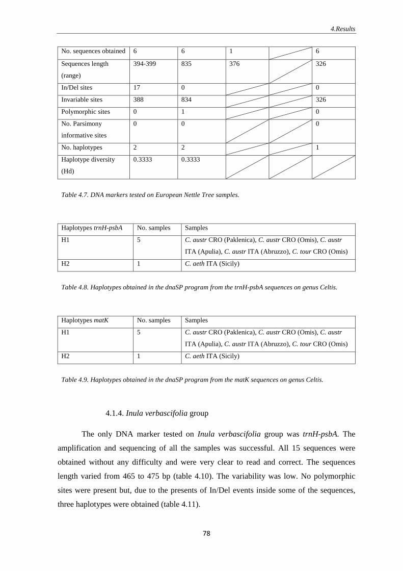
4.Results
78
No. sequences obtained 6 6 1 6
Sequences length
(range)
394-399 835 376 326
In/Del sites 17 0 0
Invariable sites 388 834 326
Polymorphic sites 0 1 0
No. Parsimony
informative sites
0 0 0
No. haplotypes 2 2 1
Haplotype diversity
(Hd)
0.3333 0.3333
Table 4.7. DNA markers tested on European Nettle Tree samples.
Haplotypes trnH-psbA No. samples Samples
H1 5 C. austr CRO (Paklenica), C. austr CRO (Omis), C. austr
ITA (Apulia), C. austr ITA (Abruzzo), C. tour CRO (Omis)
H2 1 C. aeth ITA (Sicily)
Table 4.8. Haplotypes obtained in the dnaSP program from the trnH-psbA sequences on genus Celtis.
Haplotypes matK No. samples Samples
H1 5 C. austr CRO (Paklenica), C. austr CRO (Omis), C. austr
ITA (Apulia), C. austr ITA (Abruzzo), C. tour CRO (Omis)
H2 1 C. aeth ITA (Sicily)
Table 4.9. Haplotypes obtained in the dnaSP program from the matK sequences on genus Celtis.
4.1.4. Inula verbascifolia group
The only DNA marker tested on Inula verbascifolia group was trnH-psbA. The
amplification and sequencing of all the samples was successful. All 15 sequences were
obtained without any difficulty and were very clear to read and correct. The sequences
length varied from 465 to 475 bp (table 4.10). The variability was low. No polymorphic
sites were present but, due to the presents of In/Del events inside some of the sequences,
three haplotypes were obtained (table 4.11).
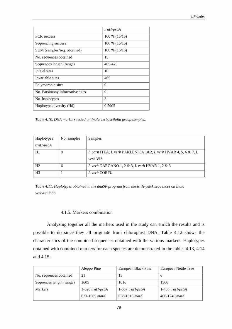
4.Results
79
trnH-psbA
PCR success 100 % (15/15)
Sequencing success 100 % (15/15)
SUM (samples/seq. obtained) 100 % (15/15)
No. sequences obtained 15
Sequences length (range) 465-475
In/Del sites 10
Invariable sites 465
Polymorphic sites 0
No. Parsimony informative sites 0
No. haplotypes 3
Haplotype diversity (Hd) 0.5905
Table 4.10. DNA markers tested on Inula verbascifolia group samples.
Haplotypes
trnH-psbA
No. samples Samples
H1 8 I. parn ITEA, I. verb PAKLENICA 1&2, I. verb HVAR 4, 5, 6 & 7, I.
verb VIS
H2 6 I. verb GARGANO 1, 2 & 3, I. verb HVAR 1, 2 & 3
H3 1 I. verb CORFU
Table 4.11. Haplotypes obtained in the dnaSP program from the trnH-psbA sequences on Inula
verbascifolia.
4.1.5. Markers combination
Analyzing together all the markers used in the study can enrich the results and is
possible to do since they all originate from chloroplast DNA. Table 4.12 shows the
characteristics of the combined sequences obtained with the various markers. Haplotypes
obtained with combined markers for each species are demonstrated in the tables 4.13, 4.14
and 4.15.
Aleppo Pine European Black Pine European Nettle Tree
No. sequences obtained 21 15 6
Sequences length (range) 1605 1616 1566
Markers 1-620 trnH-psbA
621-1605 matK
1-637 trnH-psbA
638-1616 matK
1-405 trnH-psbA
406-1240 matK
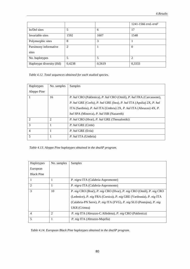
4.Results
80
1241-1566 trnL-trnF
In/Del sites 5 6 17
Invariable sites 1592 1607 1548
Polymorphic sites 8 3 1
Parsimony informative
sites
2 1 0
No. haplotypes 5 5 2
Haplotype diversity (Hd) 0,4238 0,5619 0,3333
Table 4.12. Total sequences obtained for each studied species.
Haplotypes
Aleppo Pine
No. samples Samples
1 16 P. hal CRO (Paklenica), P. hal CRO (Omiš), P. hal FRA (Carcassone),
P. hal GRE (Corfu), P. hal GRE (Itea), P. hal ITA (Apulia) 2X, P. hal
ITA (Sardinia), P. hal ITA (Umbria) 2X, P. hal ITA (Abruzzo) 4X, P.
hal SPA (Minorca), P. hal ISR (Nazareth)
2 2 P. hal CRO (Hvar), P. hal GRE (Thessaloniki)
3 1 P. hal GRE (Crete)
4 1 P. hal GRE (Evia)
5 1 P. hal ITA (Umbria)
Table 4.13. Aleppo Pine haplotypes obtained in the dnaSP program.
Haplotypes
European
Black Pine
No. samples Samples
1 1 P. nigra ITA (Calabria-Aspromonte)
2 1 P. nigra ITA (Calabria-Aspromonte)
3 10 P. nig CRO (Brač), P. nig CRO (Hvar), P. nig CRO (Omiš), P. nig CRO
(Ledenice), P. nig FRA (Corsica), P. nig GRE (Vardousia), P. nig ITA
(Calabria-PN Serre), P. nig ITA (FVG), P. nig SLO (Postojna), P. nig
UKR (Crimea)
4 2 P. nig ITA (Abruzzo-C.Alfedena), P. nig CRO (Paklenica)
5 1 P. nig ITA (Abruzzo-Majella)
Table 4.14. European Black Pine haplotypes obtained in the dnaSP program.
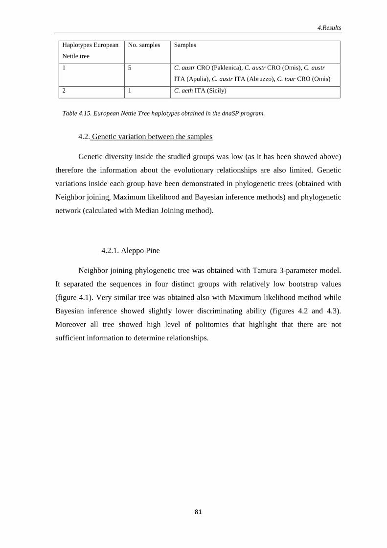
4.Results
81
4.2. Genetic variation between the samples
Genetic diversity inside the studied groups was low (as it has been showed above)
therefore the information about the evolutionary relationships are also limited. Genetic
variations inside each group have been demonstrated in phylogenetic trees (obtained with
Neighbor joining, Maximum likelihood and Bayesian inference methods) and phylogenetic
network (calculated with Median Joining method).
4.2.1. Aleppo Pine
Neighbor joining phylogenetic tree was obtained with Tamura 3-parameter model.
It separated the sequences in four distinct groups with relatively low bootstrap values
(figure 4.1). Very similar tree was obtained also with Maximum likelihood method while
Bayesian inference showed slightly lower discriminating ability (figures 4.2 and 4.3).
Moreover all tree showed high level of politomies that highlight that there are not
sufficient information to determine relationships.
Haplotypes European
Nettle tree
No. samples Samples
1 5 C. austr CRO (Paklenica), C. austr CRO (Omis), C. austr
ITA (Apulia), C. austr ITA (Abruzzo), C. tour CRO (Omis)
2 1 C. aeth ITA (Sicily)
Table 4.15. European Nettle Tree haplotypes obtained in the dnaSP program.

4.Results
82
Figure 4.1. Neighbor Joining phylogenetic tree of Aleppo Pine obtained from the trnH-
psbA and matK sequences, applying Tamura 3-parameter model.
Figure 4.2. Maximum likelihood phylogenetic tree of Aleppo Pine samples obtained from the trnH-psbA
and matK sequences with RAxML program.
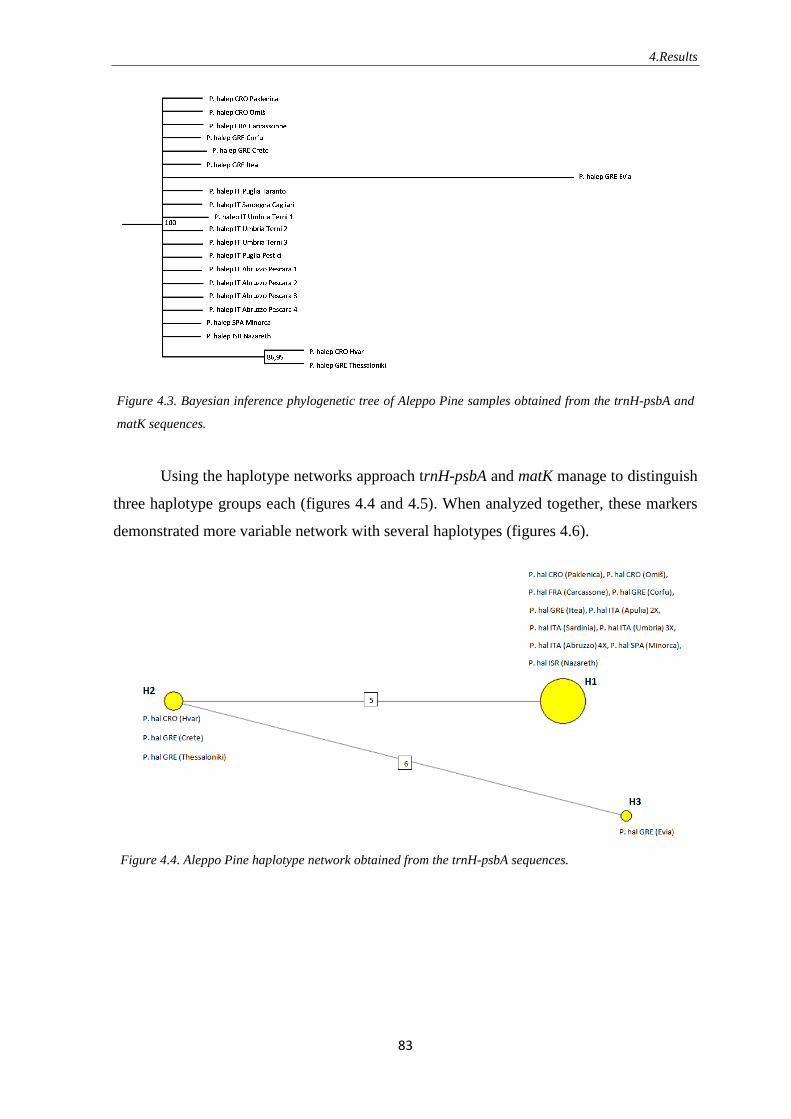
4.Results
83
Figure 4.3. Bayesian inference phylogenetic tree of Aleppo Pine samples obtained from the trnH-psbA and
matK sequences.
Using the haplotype networks approach trnH-psbA and matK manage to distinguish
three haplotype groups each (figures 4.4 and 4.5). When analyzed together, these markers
demonstrated more variable network with several haplotypes (figures 4.6).
Figure 4.4. Aleppo Pine haplotype network obtained from the trnH-psbA sequences.

4.Results
84
Figure 4.5. Aleppo Pine haplotype network obtained from the matK sequences.
Figure 4.6. Aleppo Pine haplotype network obtained from the trnH-psbA and matK sequences.
Haplotype network has been combined with the geographic map in order to
visualize the distribution of the samples and haplotypes they possess (figure 4.7). Putting
the haplotypes on the geographic map shows clearly the genetic variability inside the
eastern populations.
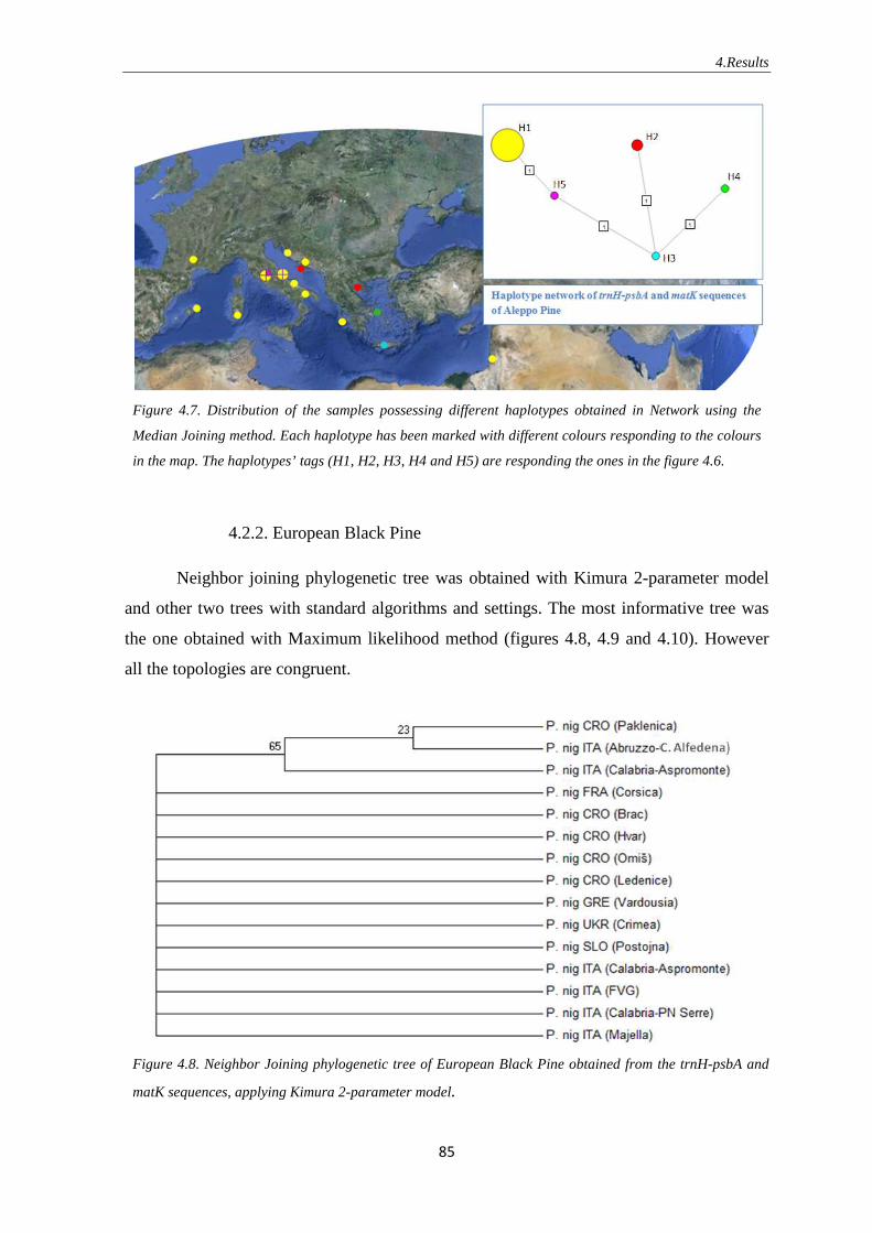
4.Results
85
Figure 4.7. Distribution of the samples possessing different haplotypes obtained in Network using the
Median Joining method. Each haplotype has been marked with different colours responding to the colours
in the map. The haplotypes’ tags (H1, H2, H3, H4 and H5) are responding the ones in the figure 4.6.
4.2.2. European Black Pine
Neighbor joining phylogenetic tree was obtained with Kimura 2-parameter model
and other two trees with standard algorithms and settings. The most informative tree was
the one obtained with Maximum likelihood method (figures 4.8, 4.9 and 4.10). However
all the topologies are congruent.
Figure 4.8. Neighbor Joining phylogenetic tree of European Black Pine obtained from the trnH-psbA and
matK sequences, applying Kimura 2-parameter model.
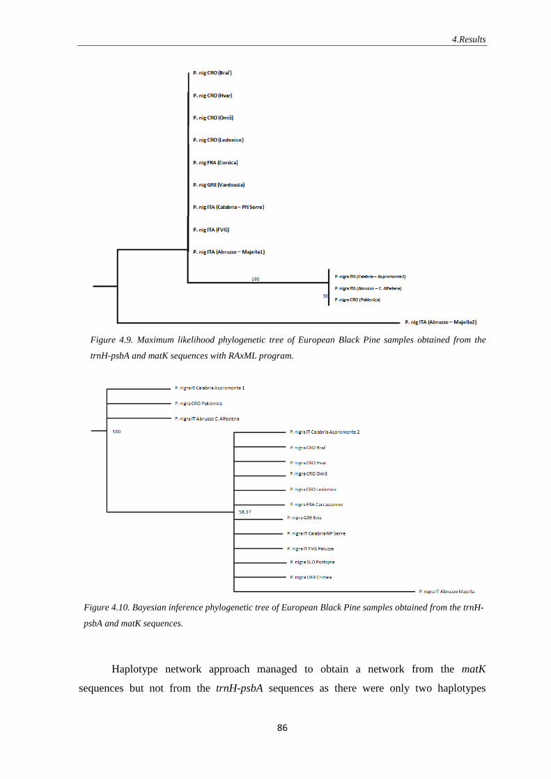
4.Results
86
Figure 4.9. Maximum likelihood phylogenetic tree of European Black Pine samples obtained from the
trnH-psbA and matK sequences with RAxML program.
Figure 4.10. Bayesian inference phylogenetic tree of European Black Pine samples obtained from the trnH-
psbA and matK sequences.
Haplotype network approach managed to obtain a network from the matK
sequences but not from the trnH-psbA sequences as there were only two haplotypes

4.Results
87
present. Combined network is more informative since it shows also the variability recorded
in trnH-psbA sequences (figures 4.11 and 4.12).
Figure 4.11. European Black Pine haplotype network obtained from the matK sequences.
Figure 4.12. European Black Pine haplotype network obtained from the trnH-psbA and matK sequences.
Haplotype network has been combined with the geographic map in order to visualize
the distribution of the samples, their appurtenance to one of the subspecies (subsp.
nigra, subsp pallasiana, subsp. dalmatica, subsp laricio) and haplotypes they possess
(figure 4.13). In this figure the colours do not present the haplotypes, as in the previous
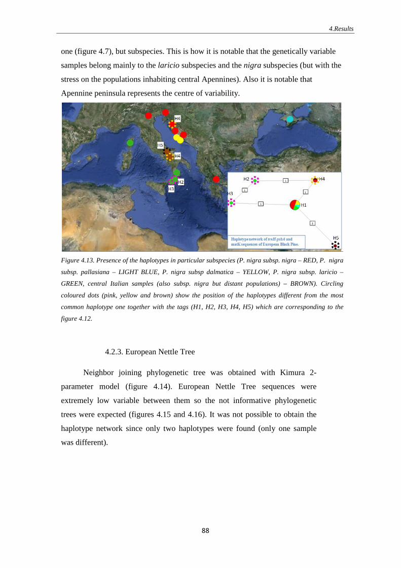
4.Results
88
one (figure 4.7), but subspecies. This is how it is notable that the genetically variable
samples belong mainly to the laricio subspecies and the nigra subspecies (but with the
stress on the populations inhabiting central Apennines). Also it is notable that
Apennine peninsula represents the centre of variability.
Figure 4.13. Presence of the haplotypes in particular subspecies (P. nigra subsp. nigra – RED, P. nigra
subsp. pallasiana – LIGHT BLUE, P. nigra subsp dalmatica – YELLOW, P. nigra subsp. laricio –
GREEN, central Italian samples (also subsp. nigra but distant populations) – BROWN). Circling
coloured dots (pink, yellow and brown) show the position of the haplotypes different from the most
common haplotype one together with the tags (H1, H2, H3, H4, H5) which are corresponding to the
figure 4.12.
4.2.3. European Nettle Tree
Neighbor joining phylogenetic tree was obtained with Kimura 2-
parameter model (figure 4.14). European Nettle Tree sequences were
extremely low variable between them so the not informative phylogenetic
trees were expected (figures 4.15 and 4.16). It was not possible to obtain the
haplotype network since only two haplotypes were found (only one sample
was different).
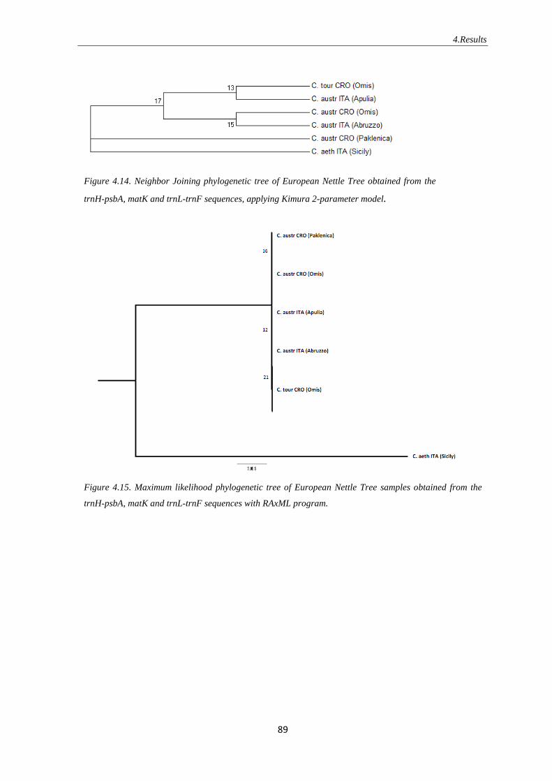
4.Results
89
Figure 4.14. Neighbor Joining phylogenetic tree of European Nettle Tree obtained from the
trnH-psbA, matK and trnL-trnF sequences, applying Kimura 2-parameter model.
Figure 4.15. Maximum likelihood phylogenetic tree of European Nettle Tree samples obtained from the
trnH-psbA, matK and trnL-trnF sequences with RAxML program.
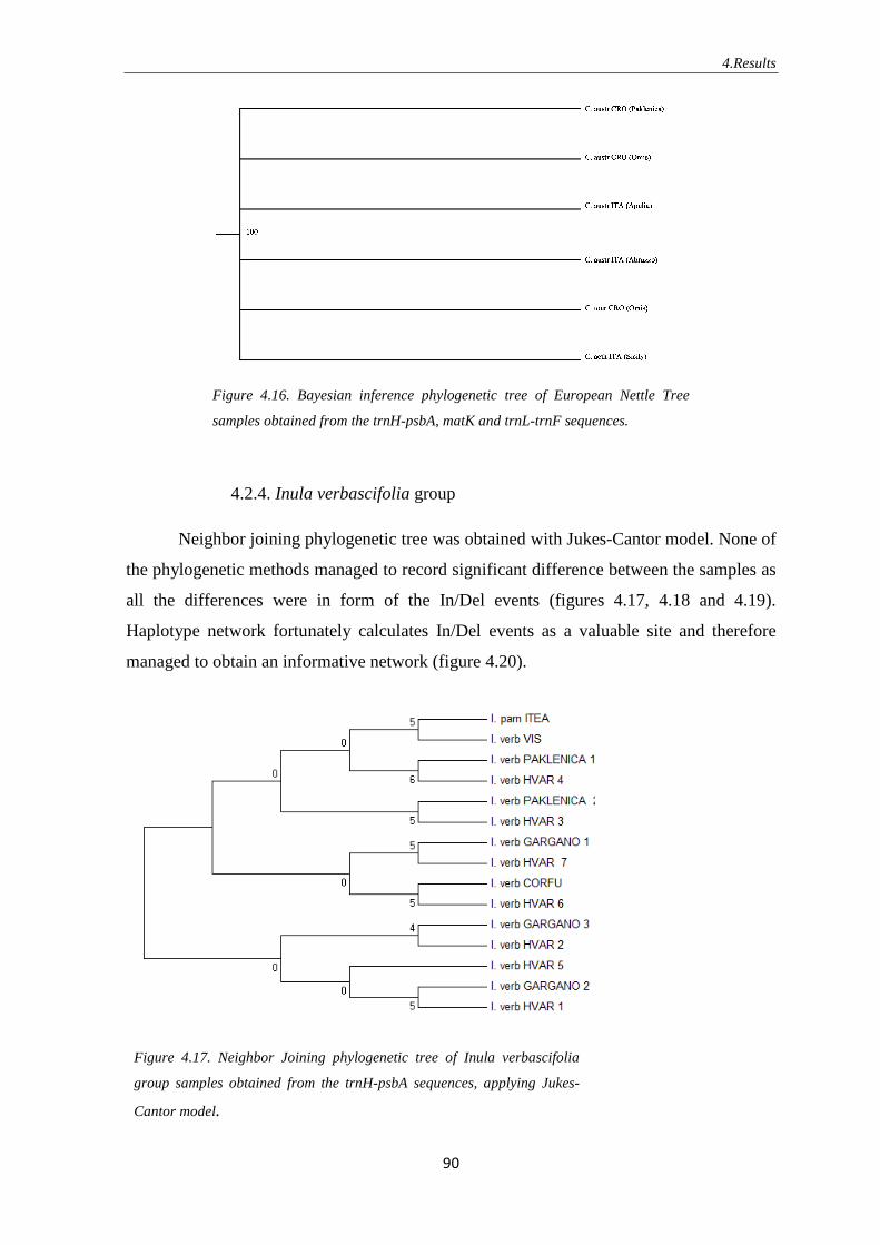
4.Results
90
Figure 4.16. Bayesian inference phylogenetic tree of European Nettle Tree
samples obtained from the trnH-psbA, matK and trnL-trnF sequences.
4.2.4. Inula verbascifolia group
Neighbor joining phylogenetic tree was obtained with Jukes-Cantor model. None of
the phylogenetic methods managed to record significant difference between the samples as
all the differences were in form of the In/Del events (figures 4.17, 4.18 and 4.19).
Haplotype network fortunately calculates In/Del events as a valuable site and therefore
managed to obtain an informative network (figure 4.20).
Figure 4.17. Neighbor Joining phylogenetic tree of Inula verbascifolia
group samples obtained from the trnH-psbA sequences, applying Jukes-
Cantor model.

4.Results
91
Figure 4.18. Maximum likelihood phylogenetic tree of Inula verbascifolia
group samples obtained from the trnH-psbA sequences with RAxML
program.
Figure 4.19. Bayesian inference phylogenetic tree of Inula verbascifolia group samples obtained from the
trnH-psbA sequences.
Figure 4.20. Inula verbascifolia haplotype network obtained from the trnH-psbA sequences.

4.Results
92
Haplotype data were combined with the geographic map showing the position of
the samples (figure 4.21). Different populations have been signed with different colours
and these colours were later put in the haplotype network in order to show which
populations share the same haplotype. On the island of Hvar there have been sampled more
than one small populations and one of them (the one with the samples: I. verb HVAR 1, I.
verb HVAR 2 and I. verb HVAR 3) turned out to possess the different haplotype. The
enlarged window shows at precise position (orange circle) where these three samples,
possessing the H2 haplotype, grew (data not shown in the introduction but recorded in the
study).
Figure 4.21. Geographic distribution of the populations of Inula verbascifolia group. Each population is
signed with different colour, which are responding to the ones in the haplotype network. The precise
position of the samples possessing particular haplotype (H2) are shown in the enlarged map and signed
with the orange circle.
4.3. Genetic position of the studied species
In order to enrich and confirm obtained results additional sequences were taken
from the NCBI GenBank. From this part of study it is possible to see how common is
particular genera and particular marker inside the GenBank and it is possible to obtain a
wider phylogenetic vision of the studied species.
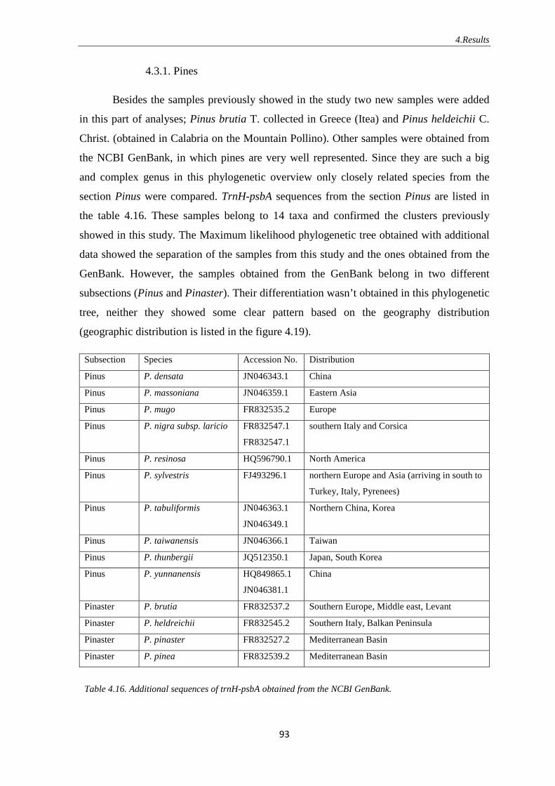
4.Results
93
4.3.1. Pines
Besides the samples previously showed in the study two new samples were added
in this part of analyses; Pinus brutia T. collected in Greece (Itea) and Pinus heldeichii C.
Christ. (obtained in Calabria on the Mountain Pollino). Other samples were obtained from
the NCBI GenBank, in which pines are very well represented. Since they are such a big
and complex genus in this phylogenetic overview only closely related species from the
section Pinus were compared. TrnH-psbA sequences from the section Pinus are listed in
the table 4.16. These samples belong to 14 taxa and confirmed the clusters previously
showed in this study. The Maximum likelihood phylogenetic tree obtained with additional
data showed the separation of the samples from this study and the ones obtained from the
GenBank. However, the samples obtained from the GenBank belong in two different
subsections (Pinus and Pinaster). Their differentiation wasn’t obtained in this phylogenetic
tree, neither they showed some clear pattern based on the geography distribution
(geographic distribution is listed in the figure 4.19).
Subsection Species Accession No. Distribution
Pinus P. densata JN046343.1 China
Pinus P. massoniana JN046359.1 Eastern Asia
Pinus P. mugo FR832535.2 Europe
Pinus P. nigra subsp. laricio FR832547.1
FR832547.1
southern Italy and Corsica
Pinus P. resinosa HQ596790.1 North America
Pinus P. sylvestris FJ493296.1 northern Europe and Asia (arriving in south to
Turkey, Italy, Pyrenees)
Pinus P. tabuliformis JN046363.1
JN046349.1
Northern China, Korea
Pinus P. taiwanensis JN046366.1 Taiwan
Pinus P. thunbergii JQ512350.1 Japan, South Korea
Pinus P. yunnanensis HQ849865.1
JN046381.1
China
Pinaster P. brutia FR832537.2 Southern Europe, Middle east, Levant
Pinaster P. heldreichii FR832545.2 Southern Italy, Balkan Peninsula
Pinaster P. pinaster FR832527.2 Mediterranean Basin
Pinaster P. pinea FR832539.2 Mediterranean Basin
Table 4.16. Additional sequences of trnH-psbA obtained from the NCBI GenBank.

4.Results
94
Figure 4.19. Maximum Likelihood phylogenetic tree obtained with trnH-psbA sequences in RAxML
program. Sequences in red are the ones produced in this study and the black ones were obtained from the
NCBI GenBank.
MatK sequences of genus pine are more represented in GenBank than the ones of
trnH-psbA so it was possible to perform a more detailed analysis. Once again the
phylogenetic study was restricted to the Pinus section, but this time with more sequences
included (table 4.17). Maximum likelihood phylogenetic tree resolved more branches than
the previous one (obtained with trnH-psbA sequences) and this time distinguished well the

4.Results
95
two subsections (Pinus and Pinaster). Once again the samples from this study got well
clustered in aspect the ones obtained from the GenBank (figure 4.20).
Subsection Species Accession No. Distribution
Pinus P. densata JF955508.1 China
Pinus P. densiflora JF955542.1 Eastern Asia
Pinus P. hwangshanensis AB161007.1 China
Pinus P. kesiya AB161008.1 Eastern Asia
Pinus P. massoniana JF955528.1 Eastern Asia
Pinus P. merkusii AB019848.1 southeast Asia
Pinus P. nigra AB084498.1 DQ353717.1
AB019854.1 Mediterranean Basin
Pinus P. resinosa AY497288.1 North America
Pinus P. sylvestris JF955488.1 northern Europe and Asia (arriving in
south to Turkey, Italy, Pyrenees)
Pinus P. tabuliformis JF955518.1 Northern China, Korea
Pinus P. taiwanensis JF955536.1 Taiwan
Pinus P. thunbergii JF955548.1 JQ512470.1 Japan, South Korea
Pinus P. tropicalis AB080920.1 Cuba
Pinus P. yunnanensis JF955554.1 China
Pinaster P. brutia AB161018.1 AB019857.1 Southern Europe, Middle east, Levant
Pinaster P. canariensis AB084494.1 Canary Islands
Pinaster P. halepensis AB019856.1 Mediterranean Basin
Pinaster P. heldreichii AB161006.1 Southern Italy, Balkan Peninsula
Pinaster P. pinaster AB084493.1 Mediterranean Basin
Pinaster P. pinea AB084496.1 Mediterranean Basin
Pinaster P. roxburghii AB019861.1 Himalayas
Table 4.17. Additional matK sequences obtained from the NCBI GenBank.

4.Results
96
Figure 4.19. Maximum Likelihood phylogenetic tree obtained with matK sequences in RAxML program.
Sequences in red are the ones produced in this study and the black ones were obtained from the NCBI
GenBank.
4.3.2. Genus Celtis
Genus Celtis (consisting of around 70 species) has been rarely studied on the
genetic level, therefore only 324 sequences from whole genus could be found in the
GenBank. TrnH-psbA sequences of only three different species were present. More

4.Results
97
supported were the sequences of other two markers (eight matK and nine trnL-trnF
sequences) (tables 4.18 and 4.19). Phylogenetic trees obtained from these two markers
were very different. While the one based on matK (figure 4.20) resolved all the inter-
specific variations with the bootstrap value of 100%, trnL-trnF tree (figure 4.21) just
managed to distinguish South American species from all the others.
Species Accession No. Distribution
Celtis occidentalis L. AY257535.1 North America
Celtis iguanaea (Jacq.) Sarg JQ589366.1 Central and south America
Celtis africana N.L.Burm. JF270686.1 Southern Africa
Celtis sinensis Pers. HQ427397.1 Eastern Asia
Celtis australis subsp. australis HE967374.1 Europe, Asia
Celtis tetrandra Roxburgh JF317420.1 Asia
Celtis schippii L. GQ981961.1 South America
Celtis philippensis Bl. AY263925.1 Southern Africa, India, Indonesia, Australia
Table 4.18. Additional matK samples taken from the NCBI GenBank.
Species Accession No. Distribution
Celtis sellowiana Miq. JN040365.1 Central and south America
Celtis iguanaea (Jacq.) Sarg AY488673.1
JN040361.1 Central and south America
Celtis sinensis Pers. JN040366.1 Eastern Asia
Celtis tournefortii var. aetnensis HE967374.1 Sicily, Europe
Celtis tala Gillet ex Planch. JN040367.1 South America
Celtis biondii Pamp. JN040363.1 China
Celtis philippensis Bl. AY147093.1 Southern Africa, India, Indonesia, Australia
Celtis madagascariensis Sattarian JN040364.1 Madagascar
Table 4.19. Additional trnL-trnF samples taken from the NCBI GenBank.
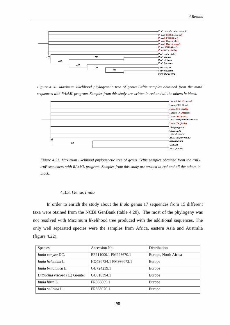
4.Results
98
Figure 4.20. Maximum likelihood phylogenetic tree of genus Celtis samples obtained from the matK
sequences with RAxML program. Samples from this study are written in red and all the others in black.
Figure 4.21. Maximum likelihood phylogenetic tree of genus Celtis samples obtained from the trnL-
trnF sequences with RAxML program. Samples from this study are written in red and all the others in
black.
4.3.3. Genus Inula
In order to enrich the study about the Inula genus 17 sequences from 15 different
taxa were otained from the NCBI GenBank (table 4.20). The most of the phylogeny was
not resolved with Maximum likelihood tree produced with the additional sequences. The
only well separated species were the samples from Africa, eastern Asia and Australia
(figure 4.22).
Species Accession No. Distribution
Inula conyza DC. EF211000.1 FM998670.1 Europe, North Africa
Inula helenium L. HQ596734.1 FM998672.1 Europe
Inula britannica L. GU724259.1 Europe
Dittrichia viscosa (L.) Greuter GU818394.1 Europe
Inula hirta L. FR865069.1 Europe
Inula salicina L. FR865070.1 Europe
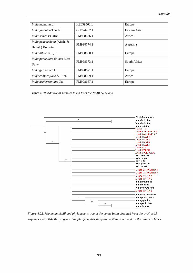
4.Results
99
Inula montana L. HE659560.1 Europe
Inula japonica Thunb. GU724262.1 Eastern Asia
Inula shirensis Oliv. FM998676.1 Africa
Inula peacockiana (Aitch. &
Hemsl.) Korovin FM998674.1 Australia
Inula bifrons (L.)L. FM998668.1 Europe
Inula paniculata (Klatt) Burtt
Davy FM998673.1 South Africa
Inula germanica L. FM998671.1 Europe
Inula confertiflora A. Rich FM998669.1 Africa
Inula aschersoniana Jka FM998667.1 Europe
Table 4.20. Additional samples taken from the NCBI GenBank.
Figure 4.22. Maximum likelihood phylogenetic tree of the genus Inula obtained from the trnH-psbA
sequences with RAxML program. Samples from this study are written in red and all the others in black.

5.Discussion
100
5. DISCUSSION
5.1. Choosing a perfect DNA marker
For resolving phylogenetic problems at the species or lower levels it is necessary to
find regions of the genome with very high evolutionary rates. Utilization of a larger
number of DNA regions gives further information and minimizes the possible errors in
data interpretation. Therefore, seeking for additional regions with high evolutionary rates is
always very important for phylogenetic analyses.
One of the aims of the study was to find the most variable sites. Another way to
evaluate the marker regards its amplification rate that can vary depending on the variability
of the primer region.
1. TrnH-psbA is a highly universal marker used for standardized plant barcoding
protocols, able to amplify and sequence easily across all the lineages (Shaw et al.
2007, Pang et al. 2011, De Mattia et al. 2012). Therefore it is slightly surprising that
in this study it did not obtain 100% of sequencing success for all the species.
However, failures in pine species could be a consequence of technical issues in the
procedure (as it was the first species studied) and European Nettle Tree samples,
even though all DNA was extracted from the fresh well-state material, demonstrated
difficulties in amplifications with all the markers. The only problem reported for this
marker in literature (Dong et al. 2012, Shaw et al. 2007) is the presence of
mononucleotide repeats (poly-structures or single nucleotide microsatellites) which
can cause sequencing problems. In actual study this problem did not occur.
2. For matK it has been recorded that it is not a universal marker and exactly that is
usually the only drawback about this locus (Dunning & Savolainen 2010, Yu et al.
2011, Dong et al. 2012). Till now, there has been described an enormous number of
primers but the general experience says: if the studied group has never been studied
before it is a big possibility that the chosen primers will not work perfectly. During
the years of the research a huge number of sequences have been tested (de Vere et al.
2011, Ford et al. 2009, Koch et al. 2001). Sometimes large numbers of primers get
tested in the same study of a simple genus (Sang et al. 1997, Koch et al. 2001, Conti
et al. 1999). The most universal primers now are described by Kim (unpublished).
These are probably also the most widely used ones, especially due to the fact that
they have been recommended for DNA barcoding (Hollingsworth et al. 2011). For
5.Discussion
101
European Nettle Tree the matK KIM primers were used and despite some difficulties
managed to amplify all the samples. The sequences of the pines were obtained with a
primer described especially for the gymnosperms by Wang et al. (1999). The same
primer later got used for DNA barcoding by China Plant BOL Group (2011) but
there is also a large number of new primers that are being developed just for
gymnosperms (Li et al. 2011). To sum up, in this case the amplification success
wasn't high (48,8% for Aleppo Pine, 60% for European Black Pine, 54,5% for
European Nettle Tree), but all the sample were eventually sequenced.
3. trnT-trnL intergenic spacer, trnL introne and trnL-trnF intergenic spacer performed
perfectly (100% amplification success) when dealing with pines, but trnT-trnL failed
in amplifying European Nettle Tree sequences despite the adjustment of the
temperature of the PCR and repeating the analysis. trnT-trnL is in fact the less
commonly used region from the trnL complex due to its low amplification rate. This
difficulty apparently seems to be caused by the trnT primer, which Taberlet et al.
(1991), when desining the primers for whole region, called primer ‘‘A’’. A new
PCR-amplification primer designed by Cronn et al. (2002) (used also in this study)
seemed to work good in wide spectrum of species (Shaw et al. 2007) and helped
wider usage of the region. It would have been an interesting experiment to apply the
old primer designed by Taberlet on the European Nettle Tree samples, but
unfortunately we did not used it in our study.
4. trnS-trnG intergenic spacer was tested only on the samples of European Nettle Tree.
The primer used in this study (G toward S) was one of additional primers sometimes
used to amplify only the trnG intron, and for sequencing longer fragments and
templates with a difficult poly-A repeat. However, it seems that this primer is not so
universal and amplification did not have high success (PCR success 60%, sequencing
33%). After five attempts with just one satisfactory sequence, this marker was
discarded from further analysis.
5. trnS–trnQ intergenic spacer was tested on the samples of European Black Pine.
These primers were designed in 2010 by Schirone et al. in order to study
phylogeography of the genus Taxus. Due to the evolutionary closeness of the species
the primers were successfully amplified on the pine samples (50% of the sequences
were obtained). However, three sequences obtained did not show any variability,
therefore also this marker got excluded from the further studies.

5.Discussion
102
6. The biggest problem was ITS region. Use of the ITS region was interesting in this
study as it is the only non-chloroplast region in the study but unfortunately it did not
function well. For ITS region there is a great variety of applicable primers (Song et
al. 2012). Many researchers tend to design new primers covering only some parts of
the region, because the whole ITS region is long. The gymnosperms turned out to
have problems in amplification of classical markers and usage of the whole regain is
hard because of particularly long ITS1 region in this group (Gernandt & Liston
1999). In this study the primers were designed specially for the pines (Simeone
unpublished). The region which they are covering starts from the end of the ITS1
spacer, spreads over the whole 5.8S RNA and almost the whole ITS2 spacer. Apart
from some difficulties in amplification of the Aleppo Pine sequences (50% of the
PCR success) the problem was that the sequences were difficult to read so any
eventual variability was hard to take with certainty. The last reason why ITS was
eliminated from the study was the result obtained from the first six samples;
comparing these sequences there was not any variability observed between the
Aleppo Pine and European Black Pine samples. Since the intention of the study was
to find any intraspecific variability, this low variation was unacceptable for the
further analysis.
Regions used the most in this study, matK and trnH-psbA, seemed to be equally
variable within the studied groups of plants and both markers delivered generally
satisfactory results. Both regions recorded some In/Del events (trnH-psbA five between
Aleppo Pine and 17 between Celtis sequences; matK six between European Black Pine
sequences) as well as some SNPs (trnH-psbA six between Aleppo Pine and two between
European Black Pine sequences; matK two between the sequences of Aleppo Pine, one
between the European Black Pine sequences and one between Celtis genera sequences).
These differences, even though few, are significant because they are intraspecific (only in
the case of Celtis genus we were dealing with closely related species).
trnH-psbA has predominantly been used for the studies including closely related
genera but several intraspecific studies have also given good result and have shown even
the higher variability then the one expressed in this study. Cavers et al. (2013) studied the
cryptic species of the tree Cedrela odorata L. and found 17 SNPs and 6 indels, resulting in
the characterization of 17 haplotypes. Ruiz-Sanchez & Specht (2013) studied the
diversification of an endemic species Nolina parviflora and managed to obtain 24

5.Discussion
103
chloroplast marker haplotypes. Yuan et al. (2011) studied the phylogeographic structure of
the endangered tree peony and found 4 substitution sites and 2 indels. These results
generally accord with the ones from this study, suggesting that the variability of the
individuals of the complex species can be found, especially for the long distant groups.
matK is one of the most rapidly evolving plastid coding regions and it consistently
shows high levels of discrimination among angiosperm species (CBOL 2009). Still, being
a coding region, its variability is limited and some researchers think it can rarely be helpful
in separating species (Dong et al. 2012) or lower taxonomic levels. This is a reason why
not so many studies can be found in which matK region is used for studying intraspecific
variation. Patreze & Tsai (2010) have used this reagion for studying intrapopulational
genetic diversity of Araucaria angustifolia and stated that the nucleotide diversity assessed
from matK sequences was low (pi = 0.001), but it indicated the potential of this gene for
evaluating divergence among widespread populations. Brunsfeld et al. (2007) studied
phylogeography of Salix melanopsis and analyzing the sequences of matK and rpl16
managed to demonstrate the existence of three genetic races. Houliston & Olson (2006)
studied evolution of organelle genes in Silene vulgaris and found 9 variable sites in matK
sequence. Also in this study the variability was considerable and it can be said that is was
as high as the one of trnH-psbA spacer. This is not surprising for the genus Pinus because
Wang et al. (1999) already used the matK region to study the evolution of Eurasian pines
and found out that matK sequences suggested a distinctly higher rate of evolution and that
the variation was even higher than the one of the noncoding regions. From this point of
view there is no evidence to prefer trnH-psbA over matK for future similar intraspecific
studies. The only possible problem one must always keep in mind when choosing between
these two regions is, already discussed, low amplification rate of the matK primers.
5.2. Application of the molecular methods for reconstructing of phylogenetic trees
Phylogenetic trees for each species were obtained with three different phylogenetic
methods; Neighbor Joining, Maximum likelihood and Bayesian inference. Genetic
variability among the sequences of the studied species was low, so the differences between
the phylogenetic trees based on different methods were few. One of the classifications of
the mentioned methods is usually the time and resources they require. In this case
requirements were not measurable due to the simplicity of the tasks; all the computations
were almost instantly done. However, it seemed that the biggest number of the clades was
5.Discussion
104
produced using the Maximum likelihood method, usually also supported with the highest
bootstrap values. They were followed by the Bayesian inference phylogenetic trees which
produced all the same clades but with lower bootstrap values. Neighbor Joining method
turned out to be the less informative in all the cases and with lower bootstrap values.
However the topologies are the same for all phylogenetic inferences.
Phylogenetic networks approach can be more informative for such a study. The number of
differentiations that were shown was higher than the one obtained with phylogenetic trees.
Furthermore, haplotype network in some cases (Aleppo pine network produced from the
marker combination) offered more evolutionary information than the phylogenetic trees
and suggested the ancestral haplotype.
5.3. Phylogenetic results obtained
Many plant species evolved via adaptive radiations or explosive patterns of
speciation, have evolutionary histories of only a few million years. The very short
evolutionary histories result in low sequence divergence (Dong et al. 2012). In fact all the
samples analyzed in this study are probably recently evolved taxa. This could be assumed
by their disjuct distribution which usually signalize that they live in an old glacial
refugium. They have probably arrived in that area during the last glatiations, and being in a
restricted small area isolated from the other populations, they started to accumulate
mutations which brought them to become different entities. In this case their evolution is
just about 10 000 years old, and, as Dong et al. 2012 supposed they could be taxa with low
sequences divergence.
The results obtained in this study were congruent showing vague variation of
sequences, so it is necessary to be cautious when discussing the phylogenetic patterns
based on such a recent and modest variability.
5.3.1. Aleppo Pine
Aleppo Pine sequences managed to distinguish several individuals pointing out
some interesting assumptions. The strongest supported internal clade, receiving a strong
bootstrap support (figures 4.1, 4.2 and 4.3), was the one grouping the individual from the
island of Hvar (souther Croatian coast) with the one from Thessaloniki (northern Greece).
Nowadays Aleppo Pine inhabits almost whole Croatian coast but it is considered natural
5.Discussion
105
only in several southern points (among which is also the Island of Hvar) (Vidaković 1982).
Genetic similarity of the Greek Pine from the Thessaloniki with the one from the island of
Hvar could support this theory, suggesting that the only original sample from the Croatian
coast in this study is genetically close to the Greek one. This is understandable since the
Adriatic and Ionic Sea separated them from the Apennine Peninsula (important is to notice
that most of the Adriatic Sea dried out during the last Pleistocene but not the southern part
where the Aleppo Pine population used to grow). Other Aleppo Pine samples from Croatia,
based on this assumption, were planted and introduced in the past and it is highly possible
that they were also introduced from the Italian populations.
In Bayesian inference only previously discussed clade was supported with bootstrap
value but other two methods managed to separate also the individual from the Greek Island
Evia as well as the samples from Crete and one from Umbria (Italy). The branches between
these samples are not strongly supported but Neighbor Joining phylogenetic tree seem to
group the Greek samples (Evia and Crete) together (bootstrap value is however just 30%).
All of these results can be seen also in the phylogenetic network obtained with both
markers (trnH-psbA and matK) (figures 4.6 and 4.7). Network result could be interpreted
saying that the sample from the Crete (haplotype H3) could have been a part of an ancestor
population of the Aleppo Pines. Similar assumption proposed also Grivet et al. (2009)
who, using chloroplast SSR markers came to the conclution that the eastern populations
should be the origin of the species from which they started colonisation towards west.
Furthermore, phylogenetic network once again confirmed the samples from the island of
Hvar and Thessaloniki to be identical (haplotype H2) and close to the sample from Crete,
but more distant from another Greek sample (Evia) (haplotype H4).
The sample from Umbria (haplotype H5) is grouped close to all non-classified
samples (haplotype H1), not showing the closeness to the eastern haplotypes. This result is
interesting regarding the curiosity mentioned in the introduction in which it was explained
that two current theories about the origin of these Umbrian populations are: a) the natural
relict population and b) the result of the ancient reforestation probably with the samples
from Middle East (Schiller & Brunori 1992). The results from this study are inclined to the
first theory. Closeness of the different haplotype (H5) to the most common one (H1) and
the result which shows that other three Umbria samples possess the common H1 haplotype
(while only one sample possesses the H5) could mean that the Umbrian population is a

5.Discussion
106
relict, well isolated population in which some genetic variations are starting to be evident
but still aren’t stabilized in the population.
5.3.2. European Black Pine
European Black Pine samples were less variable than the ones of Aleppo Pine. The
reasons for this difference probably lie in the ecology of these two species. Aleppo Pine
inhabits the disturbed habitats and often represents the pioneer species element in the flora
of a specific region. Such species should have the high mutation rate in order to adapt to
new habitats. European Black Pine inhabits more uniform sites. Even though Black Pine
deals with a big quantity of environmental stress, it usually inhabits places with relatively
homogeneous environmental conditions. Also Afzal-Rafii & Dodd (2007) dicussed these
species in a similar way stating that the Aleppo Pine probably survieved the glatiation
period in few restricted coastal sites from where it dispersed around the Mediterranean,
while for the European Black Pine they have demonstrated that the populations in
Apennine Peninsula, Sicily, Corsica, France, Spain and Djurdja Mountains in Africa
inhabited the present regions before the glaciations. Based on this, the present
Mediterranean distribution is not the result of the postglacial recolonization, so their
isolation could have been much longer. This would confirm that evolutionary strategy of
European Black Pine is not in fast adaptation, as it should be in a pioneer species.
Neighbor Joining phylogenetic tree (figure 4.8) for the Black Pine samples obtained
low bootstrap support. Maximum likelihood and Bayesian inference phylogenetic trees
(figures 4.9 and 4.10) gave more information and were also better bootstrap supported.
Both methods distinguished three particular samples from all the remaining ones (100%
bootstrap support in both phylogenetic trees); sample from the Mountain Aspromonte
(Calabria, Italy), Civitella Alfedena (Abruzzi, Italy) and the one from the NP Paklenica
(Croatia). Maximum likelihood tree also delineated the Croatian sample from the other two
Italian samples, while the Bayesian inference tree did not record this divergence. Another
interesting case was the sample from Abruzzi, obtained from NP Majella. Its variability
has been recorded with both, Maximum likelihood and Bayesian inference phylogenetic
trees; however the branch did not obtain bootstrap support in neither method.
Combined phylogenetic haplotype network (figure 4.11) showed the most frequent
haplotype (H1) to be predominant in the majority of the samples (from Croatia, Slovenia,
5.Discussion
107
France, Greece, Ukraine and in two samples from Italy), suggesting that this is the
ancestral haplotype. Other haplotypes (H2, H3, H4 and H5), basically from the Apennine
Peninsula (with the exception of one sample from NP Paklenica) are dispersed around the
H1 haplotype in the network. This haplotype pattern suggests that the highest haplotype
diversity is concentrated on the Apennine Peninsula which has confirmed to be the core of
the genetic diversity for the European Black Pine across its distribution range.
In the figure 4.12, showing the geographic distribution of the Black Pine subspecies
and the plastid haplotypes, it is possible to see that samples from the two of four studied
subspecies (P. nigra subsp. dalmatica and P. nigra subsp. pallasiana) did not shown any
variability from the rest of the samples (possess the H1 haplotype). In the other two
analysed subspecies (P. nigra subsp. nigra and P. nigra subsp. laricio) haplotype variation
was detected, but showed punctual genetic variability despite of grouping the samples
appertaining from the same subspecies in the same haplotypes. Result showed in the figure
4.12 points out that the most haplotype diversity is being present on the Apennine
Peninsula. When comparing the geography of the Apennine peninsula with the ecology of
the Black Pine it could be possible to assume that the Po Valley represented and still
represent a large barrier for the migration and dispersion of pines inhabiting the Peninsula.
Therefore it is possible that the sampled European Black Pine trees inhabiting the
Peninsula are much more isolated than all the other European Black Pines in Europe,
which could lead to genetic variability divergence of these populations and diversification
of unique haplotypes.
In the introduction we discussed the doubts about the origin of the central Italian
populations (in this study samples from the mountain Majella (H5) and from C. Alfedena
(H4)), which were finally contributed to the northern populations of P. nigra subsp. nigra
(confirmed ultimately also in microsatellite analyses by Bruschi at al. (2005).. Also this
study may confirm affilation of these samples to the nigra subspecies, especially due to the
genetic similarity of Croatian sample from NP Paklenica (H4) to the one from the C.
Alfedena. However, the variability of these populations could be suggesting that the
species, once they arrived in the current region of central Apennines, lost most of the
contact with the original population and they started their own evolution. They could have
arrived in that region even before the Pleistocene and could have started their
differentiation early. This is also the assumption of Afzal-Rafii & Dodd (2007) who
analyzed the chloroplast SSR markers and came to the conclusion that the Apenine
populations inhabited that region before the glaciations.

5.Discussion
108
5.3.3. European Nettle Tree
Samples of the genus Celtis did not show any sequence variation, except for the
sample of Celtis aethnensis from the Sicily. Low variability was also recorded by De
Castro & Maugeri (2006) who were studying the molecular variation of several
Mediterranean Celtis species. They recorded no variability inside the trnL intron but found
some differences in the ITS1 and ITS2 sequences. ITS sequences from their study
demostrated C. tournefortii as a monophyletic group (with the exception of the Iranian C.
australis entering in the C. tournefortii group); C. glabrata as a distinct species; and C.
aspera and C. aethnensis were not recognized as a distinct species but where clustered
together with C. tournefortii. In this study variability was observed in trnH-psbA and matK
sequences. All together, the sequence variability rate was extremely low, since in the
sequence 1566 bp long there were recorded only 17 In/Del sites and one mutation. No
computation method managed to obtain a well supported phylogenetic tree using these data
and phylogenetic network was impossible to obtain as only two haplotypes were detected.
Nevertheless, the result obtained in this study (but unfortunately visible only when
observing directly the sequence alignment) distinguish the sample of Celtis aethnensis
while the C. tournefortii possessed the same haplotype as C. australis. This is an
interesting result since De Castro & Maugeri (2006) had difficulties in separating C.
aethnensis but not C. tournifortii. These studies when compared could mean that all three
taxa (C. australis, C. tournifortii and C. aethnensis) present a weekly resolve clade and
their separation is not evident in many DNA regions. It should be noticed that both studies
did not obtain whole range of the species so the analyses should be performed with more
detailed sampling and including more DNA regions.
5.3.4. Inula verbascifolia group
None of the phylogenetic methods (Neighbor joining, Maximum likelihood and
Bayesian inference) managed to obtain a well supported phylogenetic tree of the Inula
verbascifolia samples (figures 4.17, 4.18 and 4.19). Still, using the phylogenetic network it
was possible to obtain three interesting haplotypes (figure 4.20 and 4.21). The first, clearly
separated, haplotype is obtained from the sample of Inula verbascifolia subsp.
verbascifolia collected in Corfu (Greece) while the other two present the mixture of the
various populations and taxa. One is formed from the samples from the Peninsula Gargano
5.Discussion
109
(Italy) and three samples from the Island of Hvar (Croatia) and the other one of all the
other samples (including the samples of Inula verbascifolia subsp. verbascifolia from the
Island of Hvar, the Island of Vis and the sample of I. verbascifolia ssp. parnassica from
Itea (Greece)). These two groups therefore did not demonstrate a clear diversification
between the distant populations, neither between the subspecies. They still showed a
genetic variability of the samples.
Before making any further assumptions, it is important to exclude the possibility
that the analysed samples from distant localities are currently exchanging the genetic
material. Inula verbascifolia is a small herbaceous plant, pollinated by the insects and
forming small dry seeds (typical for the family Asteraceae) dispersed by the wind. The
seeds do not have any adaptation on the dispersal by water and the possibility to disperse
over the Adriatic Sea seems to be impossible. The possibility that the insects make bridge
this distance across the Sea and bring the pollen from one population to the other also
seems very unlikely. Contrary to the expectations, the Croatian samples from the island of
Hvar share the same haplotype with the Italian samples. Croatian samples with this
particular haplotype all originate from the same cliff (this data are not shown in this study
but was recorded). The island of Hvar is not so close to the Apennine peninsula as the
island of Vis and the cliff with the samples possessing specific haplotype is not the locality
oriented towards Italy (figure 4.21, enlarged part of the map). Therefore, the haplotype
shared between the samples from Gargano and three from Hvar, should be the result of an
ancient, and not present, relationship between these populations. It is likely that during the
Pleistocene there were more suitable habitats for this plants around the dry Adriatic Sea
and as a result its distribution was probably much wider than today. Consequently, this
allowed the exchange of genetic material across wider geographic area and possibly
included some rare long-distance dispersion events. Genetic variation previously dispersed
on the wider territory is nowadays restricted to small populations.
These small populations probably occasionally exchange their material but based
on the occurrence of the particular haplotype in the samples growing on the same cliff
(while the other three samples from the same island, but about 50 km further located did
not possess this haplotype) suggests that the exchange is not often between these near
growing populations. However, in order to understand these movements better, it would be
necessary to perform the microsatellite analyses.

5.Discussion
110
5.4. Additional DNA sequences
Consulting the genetic results obtained from other studies is always useful and
recommended as it gives additional confirmation of the obtained results. The limiting
factor is always the richness of the database which is being used (NCBI GenBank used in
this study is the most recommended and cited one). Sequences of species used in this study
were variously represented in the database. Well represented were the pines, while the data
for the other two genera (Celtis and Inula) were poor.
Additional data can be used for two different scopes. One is confirmation of
personal results and the other is to obtain further evolutionary information. In this study all
the previously analysed species were successfully identified and classified as expected
according to existing systematic. In addition, little extra information was obtained when
using additional samples from the database.
Pine sequences obtained in this study (using DNA markers trnH-psbA and matK)
separated the Aleppo Pine and European Black Pine samples into two distinguished clades.
The correct indentification of the studied species was confirmed also by the additional
samples of the same species from the database which matched well in the phylogenetic tree
with the ones from this study. Maximum likelihood tree obtained from the trnH-psbA
sequences was not strongly supported by the bootstrap values and left more unresolved
clades. Within the phylogenetic tree there are some inconsistencies when compared with
the recent systematics (Kaundun & Lebreton 2010, Gernandt at al. 2005). Position of the
Pinus heldereichii samples was within the Black Pine clade, while in reality (based on
matK marker and molecular systematics obtained by Gernandt at al. (2005) it should be
much closely related to the Aleppo Pine. However, this classification is not strongly
supported with bootstrap values (57% and 49% respectively). MatK was more informative
marker (comparing these two phylogenetic trees). The tree based on this marker grouped
the Aleppo Pine clade and the Black Pine clade with much stronger bootstrap confirmation
and attributing them in accordance with systematic of Gernandt at al. (2005). In tree based
on matK subsection Pinaster was clearly separated from the section Pinus with the high
bootstrap value of 98%.
Samples of the genus Celtis obtained from the GenBank confirmed that the trnL-
trnF region has a very low variation in this genus. In fact, in this study this region showed
no variability whatsoever, and the comparison with the other samples confirmed its

5.Discussion
111
conserved character. The phylogenetic tree obtained from the matK sequences resolved all
the inter-specific clades with the bootstrap value of 100%. Celtis aethnensis remained the
only undistinguished sample, confirming that this species evolved recently.
Phylogenetic tree of Inula genus showed low variability of samples, except from the most
distant ones originated from South America, Africa, eastern Asia and Australia. This
confirms the assumptions that it is a relatively young clade with several closely related
species (at least in the European clade). It is however important to remember that the
studied sequence was very short and obtained with only one marker.
6.High Resolution Melting (HRM) Analysis
112
6. HIGH RESOLUTION MELTING (HRM) ANALYSES
6.1. Introduction
As it has been shown molecular analyses performed in this study are relatively long
and expensive. This type of analyses requires a big number of samples and this comes to
be the first expense in the study. The next big expense turns out to be the temptations to
sequence as much DNA regions as possible. Utilization of a larger number of DNA regions
can minimize the noise of the evolutionary heterogeneity of genes or parts of a gene. It also
minimizes the possibility of misunderstanding results caused by the factors such are
homoplasy and reticulation events. Another problem occurring is plastid capture for which
it is always recommended to combine different DNA (nuclear, mitochondrial or
chloroplast DNA). The trend of using more and more regions is well notable in the
phylogenetic studies in ultimate years (already discussed in the introduction). However,
this study, as well as the most of them, has shown misbalance between the DNA regions.
This misbalance is present in amplification rate, sequencing success and genetic variability
of the regions applied on different species. They are the cause of the big looses for the
researcher who is starting a new phylogenetic complex.
The biggest cost and also the most time-consuming part in this study was the DNA
sequencing as our laboratory didn’t posses the equipment to perform it. Therefore it was
neccessary to send purified DNA material in sequencing laboratories (Eurofins MWG
Operon and Macrogen Inc. (Europe)). This made the sequencing relatively costly process,
and forced us to revaluate thoroughly each tested marker based on few trial samples,
before submitting the rest of specimens to sequencing. Of course this exclusion-method
that was used may have caused the loss of potentially interesting information
An effective way to reduce the sequencing costs is offered with a method called
High Resolution Melting (HRM). Using this technique a researcher is able to find
unknown mutations or modifications, during a post-amplification melting curve
experiment. The methodology was first introduced by Ririe et al. (1997) and turned out to
be particularly precise in spotting the small sequence differences. Classic PCR
amplification is being enriched by adding the florescent dyes (SYBR Green I). After the
amplification, the melting process involves the programmed increase of temperature to
dissociate the amplified double-strand DNA amplicons. If the fluorescence of SYBR Green
6.High Resolution Melting (HRM) Analysis
113
I is monitored continuously throughout a temperature cycle, product denaturation can be
observed as a rapid loss of fluorescence near the denaturation temperature. The decline of
fluorescence against real-time increase in temperature can be shown in the melting curve.
Since the melting curve of a product is dependent on its GC content, length and sequence
melting curves can point out samples which differ from the others. So, this instrument
doesn’t show the entire sequence of the sample but is able to point out the samples with
particular genotype (even when the difference is just in one DNA base). The things
required are PCR reagents, a simple primer pair for amplifying the gene of interest, a
saturating DNA-binding dye, and an instrument with precise temperature control (in this
study Roche The LightCycler® 480 was used).
This is a new methodology. Most of the studies applying HRM are under the
domain of biomedicine (where special interest is being put on HRM use in diagnostics)
and, more recently, it is starting to be used also in agronomy. Its great and growing
application was found in detecting species and varieties of species (Hwang et al. 2011) but
also in authentication of the alimentary (Faria et al. 2013, Ganopoulos et al. 2012,
Ganopoulos1 et al. 2013, Kluga et al. 2013), or other commercial products (wood
authentication tested by Ganopoulos2 et al. in 2013). Recently the combination of plant
DNA barcoding with high resolution melting analysis (Bar-HRM) was introduced as a new
field. Since now it has been tested on the authentication of berry species by Jaakola et al.
(2010), bean crops by Madesis et al. (2012) and lentils by Bosmali et al. (2012).
For the first time HRM analysis has been performed as a method for one-step
haplotype identification in phylogeographic analysis (Dang et al. 2012). In their study they
combined three methods: in-vitro HRM, in-silico HRM and RFLP. In-vitro HRM
successfully discriminated between all amplicon templates. Only one pairwise comparison
yielded no discernable HRM curve difference between haplotypes, and these samples
differed by one transversion (C⁄G) SNP. In-silico HRM analysis showed the results similar
to the ones obtained in-vitro while RFLP managed to distinguish much less variables.
Based on this, authors conclude that HRM represents an untapped resource in
phylogeographic analysis, and with appropriate primer design any polymorphic locus is
potentially agreeable to this single-reaction method for haplotype identification.
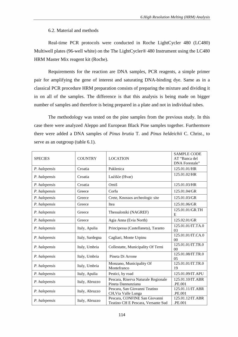
6.High Resolution Melting (HRM) Analysis
114
6.2. Material and methods
Real-time PCR protocols were conducted in Roche LightCycler 480 (LC480)
Multiwell plates (96-well white) on the The LightCycler® 480 Instrument using the LC480
HRM Master Mix reagent kit (Roche).
Requirements for the reaction are DNA samples, PCR reagents, a simple primer
pair for amplifying the gene of interest and saturating DNA-binding dye. Same as in a
classical PCR procedure HRM preparation consists of preparing the mixture and dividing it
in on all of the samples. The difference is that this analysis is being made on bigger
number of samples and therefore is being prepared in a plate and not in individual tubes.
The methodology was tested on the pine samples from the previous study. In this
case there were analyzed Aleppo and European Black Pine samples together. Furthermore
there were added a DNA samples of Pinus brutia T. and Pinus heldeichii C. Christ., to
serve as an outgroup (table 6.1).
SPECIES COUNTRY LOCATION SAMPLE CODE AT “Banca del DNA Forestale”
P. halepensis Croatia Paklenica 125.01.01/HR
P. halepensis Croatia Lučišće (Hvar) 125.01.02/HR
P. halepensis Croatia Omiš 125.01.03/HR
P. halepensis Greece Corfu 125.01.04/GR
P. halepensis Greece Crete, Knossos archeologic site 125.01.03/GR
P. halepensis Greece Itea 125.01.06/GR
P. halepensis Greece Thessaloniki (NAGREF) 125.01.01/GR.THE
P. halepensis Greece Agia Anna (Evia North) 125.02.01/GR
P. halepensis Italy, Apulia Principessa (Castellaneta), Taranto 125.01.01/IT.TA.003
P. halepensis Italy, Sardegna Cagliari, Monte Urpinu 125.01.01/IT.CA.000
P. halepensis Italy, Umbria Collestatte, Municipality Of Terni 125.01.01/IT.TR.000
P. halepensis Italy, Umbria Pineta Di Arrone 125.01.08/IT.TR.005
P. halepensis Italy, Umbria Monzano, Municipality Of Montefranco
125.01.01/IT.TR.019
P. halepensis Italy, Apulia Pestici, by road 125.01.09/IT.APU
P. halepensis Italy, Abruzzo Pescara, Riserva Naturale Regionale Pineta Dannunziana
125.01.10/IT.ABR.PE.001
P. halepensis Italy, Abruzzo Pescara, San Giovanni Teatino CH,Via Valle Lunga
125.01.11/IT.ABR.PE.001
P. halepensis Italy, Abruzzo Pescara, CONFINE San Giovanni Teatino CH E Pescara, Versante Sud
125.01.12/IT.ABR.PE.001

6.High Resolution Melting (HRM) Analysis
115
Di S. G. Teatino
P. halepensis Italy, Abruzzo Pescara, Montesilvano PE, Strada Provinciale Palmiro Togliatti
125.01.13/IT.ABR.PE.001
P. halepensis Spain, Minorca Ciutadella 125.01.01/SPA.MIN
P. halepensis Israel Tabor, Nazareth 125.01.02/IL
P. halepensis France Carcassonne 125.01.01/FRA.CAR
P. nigra subsp. dalmatica
Croatia Brac, Bol - Supetar street 129.01.01/HR.DAL
P. nigra subsp. dalmatica
Croatia Hvar 129.01.02/HR.DAL
P. nigra subsp. nigra Croatia Omiš 129.01.01/HR.NIG
P. nigra subsp. nigra Croatia Paklenica 129.01.02/HR.NIG
P. nigra subsp nigra. Croatia Ledenice 129.01.03/HR.NIG
P. nigra subsp. nigra Greece Vardousia 129.01.01/GRE.VAR
P. nigra subsp. nigra Italy, Abruzzo Civitella Alfedena 129.01.01/IT.AQ.035
P. nigra subsp. nigra Italy, F.V.G. Lusevera (UD) 129.01.01/IT.UD.051
P. nigra subsp. nigra Slovenia Postojna 129.01.01/SLO.POS
P. nigra subsp. laricio Italy, Calabria Aspromonte 129.01.01/CAL.ASP.01
P. nigra subsp. laricio Italy, Calabria Aspromonte 129.01.01/CAL.ASP.02
P. nigra subsp. laricio Italy, Calabria Serra San bruno (Vibo Valentia) 129.01/IT.VV.037
P. nigra subsp. nigra Italy, Abruzzo Majella, Fara San Martino 129.01.01/ABR.MAJ.01
P. nigra subsp. laricio France Corsica, Vallèe de la Restonica, Comune de Corte
129.01.01/FRA.CORS
P. nigra subsp. pallassiana
Ukraine Crimea, 39°27’10’’, 29°41’32’’ 129.01.01/UKR.PAL
P. brutia Greece Itea 125B.01.01./GRE.IT
P. heldreichii Italy, Calabria PN Pollino 120LEU.01.01
Table 6.1. List of the samples.
The amplified sequences for this machine are recommended to be less than 300 bp
long, since it becomes less reliable between 400 and 1000 bp (Reed & Wittwer 2004).
Most of the analyses till now have been performed using the classical DNA markers (trnL,
trnL-F, ITS, rps16 etc.), sometimes entire and sometimes particular internal parts (in order
to obtain the shorter sequence). Microsatellites (SSRs) are less used since it has been
recorded that they can obtain some inaccuracy. Still sometimes they are being use and
brought satisfactory results (Bosmali et al. 2012, Mackay et al. 2008). In this case there
were amplified two pine-specific microsatellites since they were of the right length and we

6.High Resolution Melting (HRM) Analysis
116
hoped to find higher variability than the one found till now (in the study). One of the
markers was taken from González-Martínez et al. (2004) who tested the nuclear
microsatellite transfer across Eurasian pines (between which there were Aleppo Pine and
European Black Pine). From many tested microsatellites PtTX3107 was chosen. It was
designed by Auckland et al. in 2002 and was labeled as polymorphic for both species and
was about 182 bp long. Another microsatellite sequence was taken from the study of
Vendramin et al. (1996) in which he designed 20 chloroplast microsatellites for Pinaceae.
The chosen one, Pt15169, is located in rps2 region and is 115-118 bp long. It was chosen
because it was used in considerable number of studies (European Black Pine studies by
Afzal-Rafii & Dodd 2007 and Jiménez et al 2005; Aleppo Pine studies by Bucci et al. 1998
and Grivet et al. 2009). Primers sequences are written in a table 6.2.
Marker
region Primer
Type of
DNA
Number of repeat
units
Expected
size (bp) Reference
PtTX3107 f 5’- AAACAAGCCCACATCGTCAATC-3’
nDNA (CAT)14 182 Auckland et
al. in 2002 r 5’- TCCCCTGGATCTGAGGA-3’
Pt15169 F 5’-CTTGGATGGAATAGCAGCC-3’
cpDNA (C)6(T)8A(T)8
(C)8(T)14 115-118
Vendramin et
al. (1996) r 5’-GGAAGGGCATTAAGGTCATTA-3’
Table 6.2. Primers of the selected microsatelites.
The volume of the reagents in each well of the plate is 10 µl and it contains: DNA,
primers and reagents offered in the reaction kit (LC480 HRM Master Mix reagent kit
(Roche)) (table 6.3). Reagent kit contained three tubes:
1. Master Mix, 2x concentrated (including FastStart Taq DNA Polymerase, reaction buffer,
dNTP mix (with dUTP instead of dTTP) and ResoLight high-resolution melting dye)
2. MgCl2 Stock Solution, 25 mM (to adjust MgCl2 concentration)
3. H2O, PCR-grade (to adjust the final reaction volume)
REAGENTS QUANTITY PER WELL (µl)
DNA 1,5 (20 ng/µl)
Fwd primer 0,6
Rev primer 0,6
Master Mix (green cap) 5

6.High Resolution Melting (HRM) Analysis
117
MgCl2 Stock Solution (blue cap) 1,3
H2O, PCR-grade (white cap) 1
SUM 10
Table 6.3.Quantity of the requested reagents.
The PCR procedure can be adjusted depending on the primers characteristics and
when all the settings are put the procedure is ready to start. The PCR protocol used in this
study is written in the table 6.4.
Run Protocol
Detection Format: SYBR Green 1
Pre-incubation 1 Cycle Analysis mode: None
Temperature Targets
Target
(ºC)
Acquisition
Mode
Hold (hh:mm:ss) Ramp
Rate
(ºC/s)
Acquisitions
(per ºC)
Sec
Target
(ºC)
Step
Size
(ºC)
Step
Delay
(cycles)
95 None 00:10:00 4.4 0 0 0
Amplification 52 Cycles Analysis mode : Quantification
Temperature Targets
Target
(ºC)
Acquisition
Mode
Hold (hh:mm:ss) Ramp
Rate
(ºC/s)
Acquisitions
(per ºC)
Sec
Target
(ºC)
Step
Size
(ºC)
Step
Delay
(cycles)
95 None 00:00:20 4.4 0 0 0
63 None 00:00:30 2.2 0 0 0
72 Single 00:00:30 4.4 0 0 0
Melting (HRM) 1 Cycle Analysis mode: Melting Curves
Temperature Targets
Target
(ºC)
Acquisition
Mode
Hold (hh:mm:ss) Ramp
Rate
(ºC/s)
Acquisitions
(per ºC)
Sec
Target
(ºC)
Step
Size
(ºC)
Step
Delay
(cycles)
95 None 00:01:00 4.4
63 None 00:01:00 2.2
95 Continuous 0.06 10
Cooling 1 Cycle Analysis mode: None
Temperature Targets
Target Acquisition Hold (hh:mm:ss) Ramp Acquisitions Sec Step Step

6.High Resolution Melting (HRM) Analysis
118
(ºC) Mode Rate
(ºC/s)
(per ºC) Target
(ºC)
Size
(ºC)
Delay
(cycles)
40 None 00:00:30 2.2 0 0 0
Table 6.4. The PCR program.
The analyses are being run in the machine which is instantly recording the data on
computer. After the run, the amplicots were viewed in gel electrophoresis, tested for the
signs of dirt or double strands that could cause an inappropriate melting curve.
The LightCycler® 480 Instrument Tm calling analysis software module calculates
for each sample the melting temperature, the melting peak, height, width and the area
under each melting peak. The Tm calling analysis is used to identify characteristic melting
profiles of DNA products and can be performed on any experiment that includes a melting
program. The melting temperature, or Tm, is defined as the point at which half of the DNA
is double-stranded and single-stranded. After observing the melting curves it is necessary
to compare them. Two analysis methods for high resolution melting used in this study were
temperature-shifted melting curves and difference plots, which serve to highlight
differences between individual curves relative to one of the sample melting curves plotted
as a baseline. Difference plots are useful for clustering larger numbers of samples and
allowing more distinct separation of varieties but final results were made with the
temperature-shifted melting curves.
6.3. Results and discussion
Before performing the HRM analyses four samples were sequenced with classical
sequencing method to assure that the primers function well and produce the desired
fragment. For this experiment two Aleppo Pine (P. halepensis CRO (Lučišće (Hvar)) and
P. halepensis SPA (Minorca)), and two Black Pine (P. nigra subsp. laricio IT (Calabria –
Aspromonte) and P. nigra subsp. dalmatica CRO (Hvar)) samples were tested. Both
primers produced good sequences and distinguished the two species (figure 6.5).

6.High Resolution Melting (HRM) Analysis
119
Figure 6.5. The sequences of the analyzed microsatellites. The upper sequence is produced with Pt15169 and
following one by PtTX3107 microsatellite.
HRM analyses were differently successful and in the case of the chloroplast
microsatellite, Pt15169, the amplification didn’t work well. Melting curves which were
obtained were not usable. Regarding the fact that the same primer functioned well at the
classical PCR sequencing, the failure should come from badly set up settings. The probable
explanation is that the HRM machine is slightly more sensitive than the classical PCR
machine on which we were not costumed.
The analyses with nuclear microsatellite, PtTX3107, were more satisfactory.
Clustering of the samples was first performed with difference plot method in which
software automatically showed five distinct groups inside of the samples (figure 6.6).
Based on difference plot method following groups were produced:
RED LINES: P. halepensis CRO (Paklenica), P. halepensis CRO (Lučišće (Hvar)), P. halepensis GRE
(Thessaloniki), P. halepensis GRE (Evia), P. halepensis IT (Apulia – Taranto), P. halepensis IT (Sardnia –
Cagliari), P. halepensis IT (Umbria – Terni)1, P. halepensis IT (Umbria – Terni)2, P. halepensis IT (Umbria
– Terni)3, P. halepensis IT (Apulia – Pestici), P. halepensis IT (Abruzzo – Pescara)1, P. halepensis IT
(Abruzzo – Pescara)2, P. halepensis IT (Abruzzo – Pescara)3, P. halepensis IT (Abruzzo – Pescara)4, P.
halepensis SPA (Minorca), P. halepensis ISR (Nazareth), P. halepensis FRA (Carcassonne), P. nigra subsp.
dalmatica CRO (Brač)

6.High Resolution Melting (HRM) Analysis
120
BROWN LINES: P. nigra subsp. nigra CRO (Paklenica), P. nigra subsp nigra. CRO (Ledenice), P.
nigra subsp. nigra GRE (Vardousia), P. nigra subsp. laricio IT (Calabria – Serra San bruno), P. halepensis
GRE (Itea)
GREY LINES: P. brutia GRE (Itea), P. nigra subsp. pallassiana UKR (Crimea), P. nigra subsp. nigra
CRO (Omiš)
VIOLET LINES: P. halepensis CRO (Omiš), P. halepensis GRE (Corfu), P. halepensis GRE (Crete), P.
nigra subsp. dalmatica CRO (Hvar)
YELLOW LINE: P. nigra subsp. nigra IT (Abruzzo – Majella)
Figure 6.6.Normalized Difference Plot obtained with PtTX3107 microsatellite.
These results were used as a framework for the further grouping of the samples that
was performed manually using temperature-shifted melting curves (figure 6.7). Observing
melting peaks eight groups were distinguished, from which two contained big number of
the samples and the other were smaller, containing one or few species.
GROUP 1
P. halepensis CRO (Paklenica), P. halepensis CRO (Lučišće (Hvar)), P. halepensis GRE (Thessaloniki), P.
halepensis GRE (Evia), P. halepensis IT (Apulia – Taranto), P. halepensis IT (Sardnia – Cagliari), P.

6.High Resolution Melting (HRM) Analysis
121
halepensis IT (Umbria – Terni)2, P. halepensis IT (Umbria – Terni)3, P. halepensis IT (Apulia – Pestici), P.
halepensis SPA (Minorca), P. halepensis ISR (Nazareth), P. halepensis IT (Abruzzo – Pescara)1, P.
halepensis IT (Abruzzo – Pescara)2, P. halepensis IT (Abruzzo – Pescara)3, P. halepensis IT (Abruzzo –
Pescara)4, P. halepensis FRA (Carcassonne), P. brutia GRE (Itea)
GROUP 2
P. halepensis CRO (Omiš), P. halepensis GRE (Corfu), P. halepensis GRE (Crete), P. nigra subsp.
dalmatica CRO (Hvar), P. nigra subsp. dalmatica CRO (Brač), P. nigra subsp. nigra CRO (Paklenica), P.
nigra subsp nigra. CRO (Ledenice), P. nigra subsp. laricio IT (Calabria – Serra San bruno), P. nigra subsp.
nigra IT (FVG – Lusevera)
GROUP 3
P. halepensis IT (Umbria – Terni)1, P. nigra subsp. nigra IT (Abruzzo – C.Alfedana), P. heldreichii
(Calabria – Pollino)
GROUP 4
P. nigra subsp. nigra SLO (Postojna), P. nigra subsp. laricio FRA (Corsica), P. nigra subsp. laricio IT
(Calabria – Aspromonte)
GROUP 5
P. halepensis GRE (Itea)
GROUP 6
P. nigra subsp. nigra GRE (Vardousia)
GROUP 7
P. nigra subsp. nigra CRO (Omiš)
GROUP 8
P. nigra subsp. nigra IT (Abruzzo – Majella), P. nigra subsp. pallassiana UKR (Crimea),
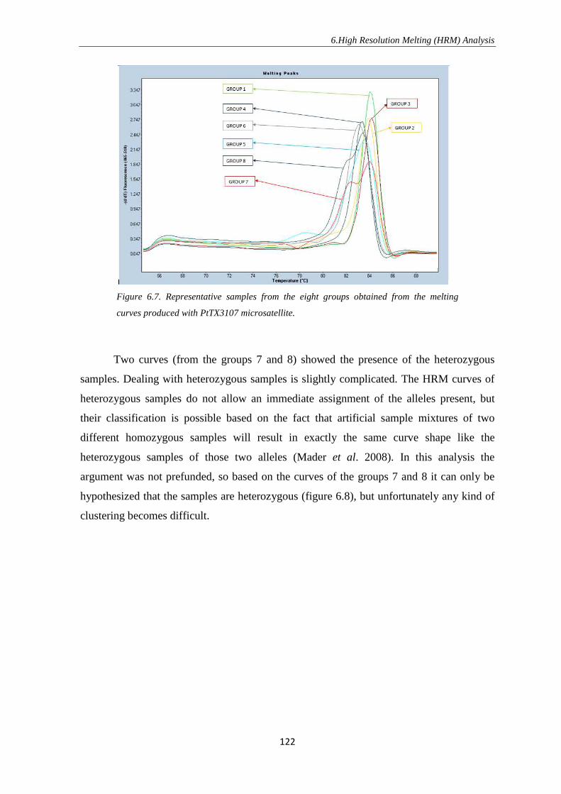
6.High Resolution Melting (HRM) Analysis
122
Figure 6.7. Representative samples from the eight groups obtained from the melting
curves produced with PtTX3107 microsatellite.
Two curves (from the groups 7 and 8) showed the presence of the heterozygous
samples. Dealing with heterozygous samples is slightly complicated. The HRM curves of
heterozygous samples do not allow an immediate assignment of the alleles present, but
their classification is possible based on the fact that artificial sample mixtures of two
different homozygous samples will result in exactly the same curve shape like the
heterozygous samples of those two alleles (Mader et al. 2008). In this analysis the
argument was not prefunded, so based on the curves of the groups 7 and 8 it can only be
hypothesized that the samples are heterozygous (figure 6.8), but unfortunately any kind of
clustering becomes difficult.
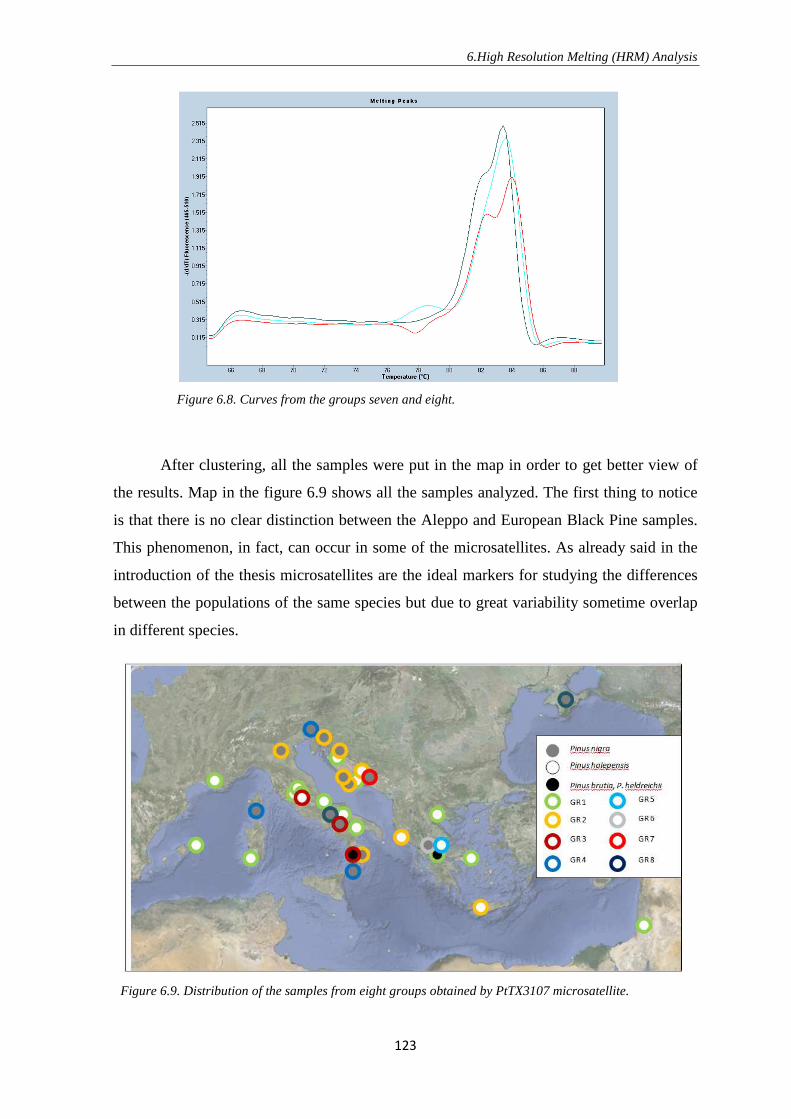
6.High Resolution Melting (HRM) Analysis
123
Figure 6.8. Curves from the groups seven and eight.
After clustering, all the samples were put in the map in order to get better view of
the results. Map in the figure 6.9 shows all the samples analyzed. The first thing to notice
is that there is no clear distinction between the Aleppo and European Black Pine samples.
This phenomenon, in fact, can occur in some of the microsatellites. As already said in the
introduction of the thesis microsatellites are the ideal markers for studying the differences
between the populations of the same species but due to great variability sometime overlap
in different species.
Figure 6.9. Distribution of the samples from eight groups obtained by PtTX3107 microsatellite.
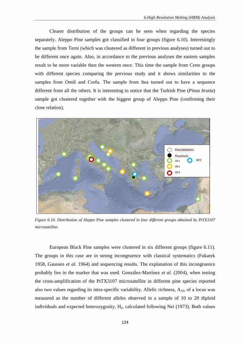
6.High Resolution Melting (HRM) Analysis
124
Clearer distribution of the groups can be seen when regarding the species
separately. Aleppo Pine samples got classified in four groups (figure 6.10). Interestingly
the sample from Terni (which was clustered as different in previous analyses) turned out to
be different once again. Also, in accordance to the previous analyses the eastern samples
result to be more variable then the western once. This time the sample from Crete groups
with different species comparing the previous study and it shows similarities to the
samples from Omiš and Corfu. The sample from Itea turned out to have a sequence
different from all the others. It is interesting to notice that the Turkish Pine (Pinus brutia)
sample got clustered together with the biggest group of Aleppo Pine (confirming their
close relation).
Figure 6.10. Distribution of Aleppo Pine samples clustered in four different groups obtained by PtTX3107
microsatellite.
European Black Pine samples were clustered in six different groups (figure 6.11).
The groups in this case are in strong incongruence with classical systematics (Fukarek
1958, Gaussen et al. 1964) and sequencing results. The explanation of this incongruence
probably lies in the marker that was used. González-Martínez et al. (2004), when testing
the cross-amplification of the PtTX3107 microsatellite in different pine species reported
also two values regarding its intra-specific variability. Allelic richness, A10, of a locus was
measured as the number of different alleles observed in a sample of 10 to 20 diploid
individuals and expected heterozygosity, He, calculated following Nei (1973). Both values

6.High Resolution Melting (HRM) Analysis
125
showed higher variability of Black Pine (A10 = 3,86; He = 0,59) samples then the ones of
Aleppo Pine (A10 = 2; He = 0,40). It results that Black Pine, as being very variable in
analyzed region, could not have been studied taking just one sample for the population.
The incongruence would probably disappear in greater sampling model, as the average
occurrence of particular samples would be different.
Figure 6.11. Distribution of Black Pine samples clustered in four different groups obtained by PtTX3107
microsatellite.
6.4. Conclusions
The problems that occur are all explainable by the selection of the markers.
Microsatellites are less recommended for HRM analyses and were not ideal for this
sampling model on such a wide area. Melting curves obtained from the PtTX3107
microsatellite region were precise, clear and simple to analyze. Unfortunately the result did
not accord with the excepted ones in the case of European Black Pine (which should, till
some point, be respected as the classical systematics has been done in high details and it
was confirmed with numerous molecular analyses). Aleppo Pine samples on the other hand
gave satisfactory results that should be evaluated by the sequencing in order to confirm
genetic variability which was supposed.
The right step to do after these analyses is to test the HRM on one of the markers
already used in this study (sequenced ones). That would serve as an objective criterion to

6.High Resolution Melting (HRM) Analysis
126
test the accuracy of this method. Since the sequences of these microsatellites were not
sequenced it is not possible to make a conclusion on whether the incongruence that
occurred for European Black Pine samples came due the inaccuracy of the HRM method or
due to the marker selection. Testing the applicability of the HRM, at this moment should
be the first scope in this type of analyses.

7.Conclusion
127
7. CONCLUSION
Clarifying the genetic systematics and genetic variability of a species is a necessary
pre-requisite towards more advanced studies concerning ecology, phylogeography, species
conservation and propagation aimed at habitat restoration. In an area so rich in species and
habitats as Mediterranean Basin all of these studies are important in order to understand,
explain and protect the present biodiversity. Conserving particular habitats and species in
the Mediterranean is especially important in the present time, considering that ongoing
climate warming might cause local extinctions, and surviving populations could be the
precious source of the genetic material. Four species studied in this thesis are just few of
many more that should be studied and appreciated in a same way.
This study has demonstrated big genetic variability among the species inhabiting
the Mediterranean Basin. This variability should be taken in consideration in wide number
of future, specialised, studies.
The great genetic variability inside the Aleppo Pine has been found in the eastern
populations, especially on the Balkan Peninsula, which should be considered the core of
this species diversity. Confirming the study from Grivet et al. (2009) analyses suggested
the Eastern Mediterranean populations as ancestor ones.
European Black Pine seems to be a species which suffered of the biggest population
loss during the last glaciations and therefore the southern populations, which remained in
their isolated refugia, are genetically pure and the most diverse. Apennine Peninsula, rich
of refugia, is an area where each population should be re-analyzed in detail, conserved and
protected from the artificial importation of the foreign genetic material.
Further on south, on the Sicily Island, there has been found particular identity of
Celtis tourniforti (informally called C. aethnensis), which demonstrated its genetic
variability comparing to the other Celtis species from the study (C. australis and C.
tournifortii).
Another area of great genetic variability is proved to be Adriatic Sea, especially
northern Adriatic coast which, on its numerous islands and islets, offers the vast number of
genetically unique populations. Opposite coasts of the Adriatic Sea showed some ancient
relationships due to which they should be always studied and compared together. Inula

7.Conclusion
128
verbascifolia subsp. verbascifolia is just one of over hundred trans-Adriatic and trans-Ionic
taxa recorded till now. As it has been seen in this study the connections are complex and
require further analyses. Understanding their past and present relationships could clarify
many questions about the Pleistocene period.
The methodology used in this study was informative and offered some new
explanations and information. Testing of such a big number of DNA regions should be
helpful in the further analyses of the same species. As it has been seen in this study
(especially in the last tested method of high resolution melting) any new technique, DNA
region and method gives additional information and enriches the infinite process of
understanding the biodiversity and evolution on our planet.
References
129
REFERENCES
Afzal-Rafii Z, Dodd RS. 2007. Chloroplast DNA supports a hypothesis of glacial refugia over
postglacial recolonization in disjunct populations of black pine (Pinus nigra) in western Europe.
Molecular Ecology. 16: 723–736.
Agarwal M, Shrivastava N, Padh H. 2008. Advances in molecular marker techniques and their
applications in plant sciences. Plant Cell Reports. 27: 617–631.
Agostini R. 1969. Le pinete di Pino d'Aleppo del Gargano. Informatore Botanico Italiano. 1: 20-21.
Aldrich J, Cherney BW, Merlin E, Christopherson L. 1988. The role of insertions/deletions in the
evolution of the intergenic region between psbA and trnH in the chloroplast genome. Current
Genetics. 14: 137–146.
Álvarez I, Wendel JF. 2003. Ribosomal ITS sequences and plant phylogenetic inference. Molecular
Phylogenetics and Evolution. 29: 417–434.
Anderberg AA. 1991. Taxonomy and phylogeny of the tribe Inuleae (Asteraceae). Plant
Systematics and Evolution. 176: 75-123.
Andersson CL, Chase MW. 2001. Phylogeny and classification of Marantaceae. Botanical Journal
of the Linnean Society. 135: 275–287.
Andersson CL, Rova JHE. 1999. The rpS16 intron and the phylogeny of the Rubioideae
(Rubiaceae). Plant Systematics and Evolution. 214: 161–186.
Applequist WL, Wallace RS. 2002. Deletions in the plastid trnT–trnL intergenic spacer define
clades within Cactaceae subfamily Cactoideae. Plant Systematics and Evolution. 231(1-4): 153-
162.
Asmussen CB, Chase MW. 2001. Coding and noncoding plastid DNA in palm systematics.
American Journal of Botany. 88(6):1103-1117.
Auckland L, Bui T, Zhou Y, Shepherd M, Williams C. 2002. Conifer microsatellite handbook.
Corporate Press, Raleigh, N.C.
Avise JC, Arnold J, Ball RM, Bermingham E, Lamb T, Neigel JE, Reeb CA, Saunders NC. 1987.
Intraspecific Phylogeography: The Mitochondrial DNA Bridge Between Population Genetics and
Systematics. Annual Review of Ecology and Systematics. 18: 489-522.
doi:10.1146/annurev.es.18.110187.002421
Azuma H, Thien LB, Kawano S. 1999. Molecular phylogeny of Magnolia (Magnoliaceae) inferred
from cpDNA sequences and evolutionary divergence of the floral scents. Journal of Plant
Research. 112: 291–306.

References
130
Baker WJ, Hedderson TA, Dransfield J. 2000. Molecular phylogenetics of subfamily Calamoideae
(Palmae) based on nrDNA ITS and cpDNA rpS16 intron sequence data. Molecular Phylogenetics
and Evolution. 14: 195–217.
Baldwin BG. 1992. Phylogenetic utility of the internal transcribed spacers of nuclear ribosomal
DNA in plants: an example from the Compositae. Molecular Phylogenetics and Evolution. 1: 3–16.
Baldwin BG. 1993. Molecular phylogenetics of Calycadenia (Compositae) based on ITS sequences
of nuclear ribosomal DNA: chromosomal and morphological evolution reexamined. American
Journal of Botany. 80: 222–238.
Ball PW, Tutin TG. 1976. Inula L. In: Tutin, TG, Heywood VH, Burges NA, Valentine DH, Walters
SM, Webb DA (eds.) Flora Europaea. Vol 4, pp. 133-136.
Barbéro M, Loisel R, Quézel P, Richardson DM, Romane F. 1998. Pines of the Mediterranean
Basin. In: Richardson DM. 1998. Ecology and Biogeography of Pinus. Cambridge University Press.
pp. 153 – 170.
Bayer RJ, Greber DG, Bagnall NH. 2002. Phylogeny of Australian Gnaphalieae (Asteraceae) based
on chloroplast and nuclear sequences, the trnL intron, trnL-trnF intergenic spacer, matK, and ETS.
Systematic Botany. 27: 801–814.
Bellstedt DU, Linder HP, Harley EH. 2001. Phylogenetic relationships in Disa based on noncoding
trnL-trnF chloroplast sequences: evidence of numerous repeat regions. American Journal of
Botany. 88: 2088–2100.
Bernetti G. 1995. Selvicoltura speciale. UTET. 132-143.
Blondel J, Aronson J. 1999. Biology and Wildlife of the Mediterranean Region. Oxford University
Press, USA. 21-34.
Bohonak AJ, Vandergast AG. 2011. The value of DNA sequence data for studying landscape
genetics. Molecular Ecology. 20: 2477–2479.
Bonavita S. 2012. Genetic diversity assessment in Pinus laricio Poiret populations using
microsatellites analysis and inferences on population hystory. Università della Calabria, Facoltà di
Scienze Matematiche, Fisiche e Naturali, Dottorato di Ricercha in Biologia Vegetale, Scuola di
Dottorato “Life Sciences”.
Borsch T, Hilu KW, Quandt D, Wilde V, Neinhuis C, Barthlott W. 2003. Noncoding plastid trnT-
trnF sequences reveal a well resolved phylogeny of basal angiosperms. Journal of Evolutionary
Biology. 16: 558–576.
Bosmali I, Ganopoulos I, Madesis P, Tsaftaris A. 2012. Microsatellite and DNA-barcode regions
typing combined with High Resolution Melting (HRM) analysis for food forensic uses: A case study
on lentils (Lens culinaris). Food Research International. 46: 141–147.
Boudraa S, Hambaba L, Zidani S, Boudraa H. 2010. Composition minérale et vitaminique des
fruits de cinq espèces sous exploitées en Algérie: Celtis australis L., Crataegus azarolus L.,
Crataegus monogyna Jacq., Elaeagnus angustifolia L. et Zizyphus lotus L.. Fruits. 65(2): 75-84.

References
131
Boys J, Cherry M, Dayanandan S. 2005. Microsatellite analysis reveals genetically distinct
population of Red pine (Pinus resinosa, Pinaceae). American Journal of Botany. 92(5): 833-841.
Bremer B, Bremer K, Heidari N, Erixon P, Olmstead RG, Anderberg AA, Källersjö M,
Barkhordarian E. 2002. Phylogenetics of asterids based on 3 coding and 3 noncoding chloroplast
DNA markers and the utility of noncoding DNA at higher taxonomic levels. Molecular
Phylogenetics and Evolution. 24: 274-301.
Brunsfeld SJ, Miller TR, Carstens BC. (2007). Insights into the biogeography of the Pacific
Northwest of North America: Evidence from the phylogeography of Salix melanopsis. Systematic
Botany. 32(1): 129-139.
Bruschi P, Di Santo D, Grossoni P, Tani C. 2005. Caratterizzazione tassonomica del Pino nero della
Majella. In: Di Cecco M., Andrisano T.: La Biodiversità vegetale nelle aree protette in Abruzzo: studi
ed esperienze a confronto (tratto dagli atti del convegno). Giardino Botanico Michele Tenore,
Lama dei Peligni (CH).
Bucci G, Anzidei M, Madaghiele A, Vendramin GG. 1998. Detection of haplotypic variation and
natural hybridization in halepensis-complex pine species using chloroplast simple sequence
repeat (SSR) markers. Molecular ecology. 7: 1633-1643.
Butterworth CA, Cota-Sanchez JH, Wallace RS. 2002. Molecular Systematics of Tribe Cacteae
(Cactaceae: Cactoideae): A Phylogeny Based on rpl16 Intron Sequence Variation. Systematic
Botany. 27(2): 257-270.
Cavers S, Telford A, Cruz FA, Perez Castaneda AJ, Valencia R, Navarro C, Buonamici A, Lowe AJ,
Vendramin GG. 2013. Cryptic species and phylogeographical structure in the tree Cedrela odorata
L. throughout the Neotropics. Journal of Biogeography. 40: 732–746.
CBOL Plant Working Group. 2009. A DNA barcode for land plants. PNAS. 106 (31): 12794-12797.
10.1073/pnas.0905845106
Chandler GT, Bayer RJ, Crisp MD. 2001. A molecular phylogeny of the endemic Australian genus
Gastrolobium (Fabaceae: Mirbelieae) and allied genera using chloroplast and nuclear markers.
American Journal of Botany. 88: 1675–1687.
Chase MW, Soltis DE, Olmstead RG, Morgan D, Les DH, Mishler BD, Duvall MR, Price RA, Hills
HG, Qiu Y, Kron KA, Rettig JH, Conti E, Palmer JD, Manhart JR, Sytsma KJ, Michaels HJ, Kress WJ,
Karol KG, Clark WD, Hedren M, Gaut BS, Jansen RK, Kim K, Wimpee CF, Smith JF, Furnier GR,
Strauss SH, Xiang Q, Plunkett GM, Soltis PS, Swensen SM, Williams SE, Gadek PA, Quinn CJ,
Eguiarte LE, Golenberg E, Learn GH Jr., Graham SW, Barrett SCH, Dayanandan S, Albert VA.
1993. Phylogenetics of Seed Plants: An Analysis of Nucleotide Sequences from the Plastid Gene
rbcL. Annals of the Missouri Botanical Garden. 80(3): 528-548 + 550-580.
Chemisquy MA, Morrone O. 2012. Molecular phylogeny of Gavilea (Chloraeinae: Orchidaceae)
using plastid and nuclear markers. Molecular Phylogenetics and Evolution. 62(3): 889-97.
References
132
Chen LY, Chen JM, Gituru RW, Temam TD, Wang QF. 2012. Generic phylogeny and historical
biogeography of Alismataceae, inferred from multiple DNA sequences. Molecular Phylogenetic
Evolution. 63(2): 407-16.
China Plant BOL Group, Li D-Z, Gao L-M, Li H-T, Wang H, Ge X-J, Liu J-Q, Chen Z-D, Zhou S-L, Chen
S-L, Yang J-B, Fu C-X, Zeng C-X, Yan H-F, Zhu Y-J, Sun Y-S, Chen S-Y, Zhao L, Wang K, Yang T, Duan
G-W. 2011. Comparative analysis of a large dataset indicates that internal transcribed spacer (ITS)
should be incorporated into the core barcode for seed plants. PNAS Early Edition. 108(49): 19641-
19646. www.pnas.org/cgi/doi/10.1073/pnas.1104551108
Chunxiao Z, Yue L, Xuemei C. 1999. The choice of isozyme markers in Pinus tabulaeformis carr.
Journal of Beijing Forestry University. 21(1): 11-16.
Clark LG, Zhang W, Wendel JF. 1995. A phylogeny of the grass family (Poaceae) based on ndhF
sequence data. Systematic Botany. 20: 436–460.
Conkle MT, Schiller G, Grunwald C. 1988. Electrophoretic Analysis of Diversity and Phylogeny of
Pinus brutia and Closely Related Taxa. Systematic Botany. 13(3): 411-424.
Conti E, Soltis DE, Hardig TM, Schneider J. 1999. Phylogenetic Relationships of the Silver
Saxifrages (Saxifraga, Sect. Ligulatae Haworth): Implications for the Evolution of Substrate
Specificity, Life Histories, and Biogeography. Molecular Phylogenetics and Evolution. 13 (3): 536–
555.
Crisp MD, Cook LG. 2011. Cenozoic extinctions account for the low diversity of extant
gymnosperms compared with angiosperms. New Phytologist. 192(4): 997–1009. DOI:
10.1111/j.1469-8137.2011.03862.x
Cronn RC, Small RL, Haselkorn T, Wendel JF. 2002. Rapid diversification of the cotton genus
(Gossypium: Malvaceae) revealed by analysis of sixteen nuclear and chloroplast genes. American
Journal of Botany. 89: 707–725.
Cuénoud P, Del Pero Martinez MA, Loizeau PA, Spichiger R, Andrews S, Manen JF. 2000.
Molecular phylogeny and biogeography of the genus Ilex L. (Aquifoliaceae). Annals of Botany. 85:
111–122.
Cuttelod A, García N, Abdul Malak D, Temple H, Katariya V. 2008. The Mediterranean: a
biodiversity hotspot under threat. In: J-C Vié, C Hilton-Taylor & SN Stuart (eds). The 2008 Review
of The IUCN Red List of Threatened Species. IUCN Gland, Switzerland.
Dang X-D, Kelleher CT, Howard-Williams E, Meade CV. 2012. Rapid identification of chloroplast
haplotypes using High Resolution Melting analysis. Molecular Ecology Resources. 12: 894–908.
De Castro O, Maugeri G. 2006. Molecular notes on the Mediterranean species of the genus Celtis
L. (Celtidaceae). Plant Biosystems. 140(2): 171-175.
De Mattia F, Gentili R, Bruni I, Galimberti A, Sgorbati S, Casiraghi M, Labra M. 2012. A multi-
marker DNA barcoding approach to save time and resources in vegetation surveys. Botanical
Journal of the Linnean Society. 169(3): 518-529.
References
133
De Peer YV. 2009. Phylogenetic inference based on distance methods. In: The Phylogenetic
Handbook: A Practical Approach to Phylogenetic Analysis and Hypothesis Testing. edt. Lemey P.,
Salemi M. Vandamme A.-M.. Cambridge University Press; 2nd edition (April 20, 2009)
De Philippis A. 1958. Varietà del Pinus nigra e reazioni del suolo. L’Alpe, XV: 2-3.
De Vere N, Rich TCG, Ford CR, Trinder SA, Long C, Moore CW, Satterthwaite D, Davies H,
Allainguillaume J, Ronca S, Tatarinova T, Garbett H, Walker K, Wilkinson MJ. 2012. DNA
Barcoding the Native Flowering Plants and Conifers of Wales. PLoS ONE 7(6): e37945.
doi:10.1371/journal.pone.0037945
Debazac EF. 1977. Manuel des conifères. Ecole Nat. Des Eaux et Forêts, Nancy, pp.172.
Del Villar EH. 1947. Quel est le nom valable du Pinus laricio Poir.. Berichte der Schweizerischen
botanischen gesellschaft. 57: 149-155.
Delevoy G. 1949. A propos de la Systématique de Pinus nigra Arnold. Travaux Station de
Recherches, Série B 12. Groenendaal, Belgique.
Demaio PH, Barfuss MH, Kiesling R, Till W, Chiapella JO. 2011. Molecular phylogeny of
Gymnocalycium (Cactaceae): assessment of alternative infrageneric systems, a new subgenus,
and trends in the evolution of the genus. American Journal of Botany. 98(11): 1841-54. doi:
10.3732/ajb.1100054.
Doebley J, Durbin M, Golenberg EM, Clegg MT, Ma DP. 1990. Evolutionary Analysis of the Large
Subunit of Carboxylase (rbcL) Nucleotide Sequence Among the Grasses (Gramineae). Evolution.
44(4): 1097-1108.
Dong W, Liu J, Yu J, Wang L, Zhou S. 2012. Highly Variable Chloroplast Markers for Evaluating
Plant Phylogeny at Low Taxonomic Levels and for DNA Barcoding. PLoS ONE 7(4): e35071.
doi:10.1371/journal.pone.0035071
Downie SR, Katz-Downie DS, Sun F-J, Lee C-S. 2008. Phylogeny and biogeography of Apiaceae
tribe Oenantheae inferred from nuclear rDNA ITS and cpDNA psbl-5’trnK (UUU) sequences, with
emphasis on the North American Endemics clade. Botany. 86: 1039-1064.
Downie SR, Katz-Downie DS, Watson MF. 2000. A phylogeny of the flowering plant family
Apiaceae based on chloroplast DNA rpl16 and rpoC1 intron sequences: towards a suprageneric
classification of subfamily Apioideae. American Journal of Botany. 87: 273–292.
Downie SR., Hartman RL, Jie S-F, Katz-Downie DS. 2002. Polyphyly of the spring-parsleys
(Cymopterus): molecular and morphological evidence suggests complex relationships among the
perennial endemic genera of western North American Apiaceae. Canadian Journal of Botany. 80:
1295–1324.
Dunning LT, Savolainen V. 2010. Broad-scale amplification of matK for DNA barcoding plants, a
technical note. Botanical Journal of the Linnean Society. 164: 1–9.
Edgar RC. 2004. "MUSCLE: a multiple sequence alignment method with reduced time and space
complexity". BMC Bioinformatics. 5(1): 113. doi:10.1186/1471-2105-5-113
References
134
Editorial Committee of the Administration Bureau of Chinese Flora. 1979. Science Press. Beijing,
Vol. 75.
Ehrendorfer F, Manen JF, Natali A. 1994. cpDNA intergene sequences corroborate restriction site
data for reconstructing Rubiaceae phylogeny. Plant Systematics and Evolution. 190: 245–248.
Eldenäs P, Anderberg AA, Källersjö M. 1998. Molecular phylogenetics of the tribe Inuleae s.
str.(Asteraceae), based on ITS sequences of nuclear ribosomal DNA. Plant Systematics and
Evolution. 210(3-4):159-173.
Fady-Welterlen B. 2005. Is There Really More Biodiversity in Mediterranean Forest Ecosystems?
Taxon. 54(4): 905-910.
Faria MA, Magalhães A, Nunes ME, Oliveira MBPP. 2013. High resolution melting of trnL
amplicons in fruit juices authentication. Food Control. 33: 136–141.
Fehrer J, Krak K, Chrtek J. 2009. Intra-individual polymorphism in diploid and apomictic polyploid
hawkweeds (Hieracium, Lactuceae, Asteraceae): disentangling phylogenetic signal, reticulation,
and noise. BMC Evolutionary Biology. 9: 239. doi:10.1186/1471-2148-9-239
Felsenstein J. 1981. "Evolutionary trees from DNA sequences: a maximum likelihood approach".
Journal of Molecular Evolution. 17(6): 368–376.
Filppula S, Szmidt AE, Savolainen O. 1992. Genetic comparison between Pinus sylvestris and P.
mugo using isozymes and chloroplast DNA. Nordic Journal of Botany. 12(4): 381–386.
Ford CS, Ayres KL, Toomey N, Haider N, Van Alphen Stahl J, Kelly LJ, Wikström N, Hollingsworth
PM, Duff RJ, Hoot SB, Cowan RS, Chase MW, Wilkinson MJ. 2009. Selection of candidate coding
DNA barcoding regions for use on land plants. Botanical Journal of the Linnean Society. 159: 1–11.
doi: 10.1111/j.1095-8339.2008.00938.x
Friesen N, Fritsch RM, Pollner S, Blattner FR. 2000. Molecular and morphological evidence for an
origin of the aberrant genus Milula within the Himalayan species of Allium (Alliaceae). Molecular
Phylogenetics and Evolution. 17: 209–218.
Fukarek P. 1958. Prilog Poznavanju crnog bora (Pinus nigra Arn. S. lat.). Radovi Poljoprivredno-
sumarskog Fakulteta B. Sumarstvo 3. Sarajevo. pp: 3-92.
Fukarek P. 1959. Bor, Šumarska enciklopedija 1, Leksikografski zavod FNRJ. pp. 101.
Fukuda T, Yokoyama J, Tsukaya H. 2003. Phylogenetic relationships among species in the genera
Chisocheton and Guarea that have unique indeterminate leaves as inferred from sequences of
chloroplast DNA. International Journal of Plant Sciences. 164: 13–24.
Galtier N, Gouy M, Gautier C. 1996. SEAVIEW and PHYLO_WIN: two graphic tools for sequence
alignment and molecular phylogeny. Computer Applications in the Biosciences. 12:543-548.
Ganopoulos2 I, Aravanopoulos F, Madesis P, Pasentsis K, Bosmali I, Ouzounis C, Tsaftaris A. 2013
Taxonomic Identification of Mediterranean Pines and Their Hybrids Based on the High Resolution

References
135
Melting (HRM) and trnL Approaches: From Cytoplasmic Inheritance to Timber Tracing. PLoS ONE
8(4): e60945. doi:10.1371/journal.pone.0060945.
Ganopoulos1 I, Bazakos C, Madesis P, Kalaitzisc P, Tsaftaris A. 2013. Barcode DNA high-resolution
melting (Bar-HRM) analysis as a novel close-tubed and accurate tool for olive oil forensic use.
Journal of the Science of Food and Agriculture. DOI 10.1002/jsfa.6040.
Ganopoulos I, Tsaballa A, Xanthopoulou A, Madesis P, Tsaftaris A. 2012. Sweet Cherry Cultivar
Identification by High-Resolution-Melting (HRM) Analysis Using Gene-Based SNP Markers. Plant
Molecular Biology Reporter. DOI 10.1007/s11105-012-0538-z
Gaskin JF, Schaal BA. 2003. Molecular phylogenetic investigation of U.S. Invasive Tamarix.
Systematic Botany. 28: 86–95.
Gaussen H, Haywood VH, Chater AO. 1964. Pinus. In: Flora Europaea, Vol. 1 (ed. Tutin TG), pp.
32–35. Cambridge University Press, Cambridge, UK.
Ge S, Li A, Lu BR, Zhang SZ, Hong DY. 2002. A phylogeny of the rice tribe Oryzeae (Poaceae) based
on matK sequence data. American Journal of Botany. 89: 1967–1972.
Gellini R, Grossoni P. 1996. Botanica forestale / Gimnosperme. CEDAM. 160-170.
Gellini R. 1968. Posizione sistematica del pino nero di Villetta Barrea in base ai caratteri anatomici
degli aghi. Annali dell'Accademia Italiana di Scienze Forestali. XVII: 101-122.
Gerber S, Baradat P, Marpeau A, Arbez M. 1995. Geographic variation in terpene composition of
Pinus nigra Arn.. Forest genetics. 2(1): 1-10.
Gernandt DS, Liston A. 1999. Internal transcribed spacer region evolution in Larix and
Pseudotsuga (Pinaceae). American Journal of Botany. 86(5): 711-723.
Gernandt DS, López GG, García SO, Liston A. 2005. Phylogeny and classification of Pinus. Taxon.
54(1): 29 – 42.
Gielly C, Yuan Y-M, Küpfer P, Taberlet P. 1996. Phylogenetic Use of Noncoding Regions in the
Genus Gentiana L.: Chloroplast trnL (UAA) Intron versus Nuclear Ribosomal Internal Transcribed
Spacer Sequences. Molecular Phylogenetics And Evolution. 5(3): 460–466.
Gielly L, Taberlet P. 1994. The use of chloroplast DNA to resolve plant phylogenies: noncoding
versus rbcL sequences. Molecular Biology and Evolution. 11: 769–777.
Giordano E, Scarascia G, Schirone B. 1984. Osservazioni sulla Rinnovazione naturale del Pino
d'Aleppo in Pulgia. Annali dell'Accademia Italiana di Scienze Forestali. 33: 273-310.
Giordano E. 1960. Osservazioni su alcuna provenienze italiane di Pinus halepensis. Centro di
Sperimentazione Agraria e Forestale. 5: 13-43.
Gola G. 1924. Sopra alcuni ibridi tra Pinus pinaster, P. halepensis e P. brutia nei dintorni di Grado.
Atti Accademia Scientifica Veneto-Trento-Istriana (Padua). 3: 72-74.
References
136
Goldblatt P, Savolainen V, Porteous O, Sostaric I, Powell M, Reeves G, Manning JC, Barraclough
TG, Chase MW. 2002. Radiation on the Cape flora and the phylogeny of peacock irises Moraea
(Iridaceae) based on four plastid DNA regions. Molecular Phylogenetics and Evolution. 25: 341–
360.
Golenberg EM, Clegg MT, Durbin ML, Doebley J, Ma DP. 1993. Evolution of a noncoding region of
the chloroplast genome. Molecular Phylogenetics and Evolution. 2: 52–64.
González-Martínez SC, Robledo-Arnuncio JJ, Collada C, Díaz A, Williams CG, Alía R, Cervera MT.
2004. Cross-amplification and sequence variation of microsatellite loci in Eurasian hard pines.
Theoretical and Applied Genetics.109(1):103-11.
Goodall-Copestake WP, Pérez-Espona S, Harris DJ, Hollingsworth PM. 2010. The early evolution
of the mega-diverse genus Begonia (Begoniaceae) inferred from organelle DNA phylogenies.
Biological Journal of the Linnean Society. 101: 243–250.
Grivet D, Sebastiani F, González-Martínez SC, Vendramin GG. 2009. Patterns of polymorphism
resulting from long-range colonization in the Mediterranean conifer Aleppo pine. New
Phytologist. 184(4): 1016-28. doi: 10.1111/j.1469-8137.2009.03015.x.
Haider N, Wilkinson MJ. 2011. A set of plastid DNA-specific universal primers for flowering plants.
Russian Journal of Genetics. 47(9): 1066-1077.
Hajibabaei M, Singer GAC, Hebert PDN, Hickey DA. 2007. DNA Barcoding: How it Complements
Taxonomy, Molecular Phylogenetics and Population Genetics. Trends in Genetics. 23(4): 167-172.
Hall TA. 1999. BioEdit: a user-friendly biological sequence alignment editor and analysis program
for Windows 95/98/NT. Nucleic Acids Symposium Series. 41:95-98.
Hanover JW. 1992. Applications of terpene analysis in forest genetics. New Forests. 6(1-4): 159-
178.
Hao DC, Huang B, Yang L. 2008. Phylogenetic relationships of the genus Taxus inferred from
chloroplast intergenic spacer and nuclear coding DNA. Biological & Pharmaceutical Bulletin. 31(2):
260–265. doi:10.1248/bpb.31.260
Hardig TM, Soltis PS, Soltis DE. 2000. Diversification of the North American shrub genus
Ceanothus (Rhamnaceae): conflicting phylogenies from nuclear ribosomal DNA and chloroplast
DNA. American Journal of Botany. 87: 108–123.
Higgins D, Lemey P. 2009. Multiple sequence alignment. In: The Phylogenetic Handbook: A
Practical Approach to Phylogenetic Analysis and Hypothesis Testing. edt. Lemey P., Salemi M.
Vandamme A.-M.. Cambridge University Press; 2nd edition (April 20, 2009)
Hilu KW, Borsch T, Müller K, Soltis DE, Soltis PS, Savolainen V, Chase MW, Powell MP, Alice LA,
Evans R, Sauquet H, Neinhuis C, Slotta TAB, Rohwer JG, Campbell CS, Chatrou LW. 2003.
Angiosperm phylogeny based on matK sequence information. American Journal of Botany. 90:
1758–1776.
References
137
Hilu KW, Liang H. 1997. The matK gene: sequence variation and application in plant systematics.
American Journal of Botany. 84: 830–839.
Hiratsuka J, Shimada H, Whittier R, Ishibashi T, Sakamoto M, Mori M, Kondo C, Honji Y, Sun CR,
Meng BY, Li YQ, Kanno A, Nishiyawa Y, Hirai A, Shinozaki K, Sigiura M. 1989. Thecomplete
sequence of the rice (Oryza sativa) chloroplast genome: intermolecular recombination between
distinct tRNA genes accounts for a major plastid DNA inversion during the evolution of the
cereals. Molecular General Genetics. 217: 185–194.
Holdregger R, Abbott RJ. 2003. Phylogeography of the Arctic Alpine Saxifraga oppositifolia
(Saxifragaceae) and some related taxa based on cpDNA and ITS sequence variation. American
Journal of Botany. 90: 931–936.
Hollingsworth PM, Graham SW, Little DP. 2011. Choosing and Using a Plant DNA Barcode. PLoS
ONE. 6(5): e19254. doi:10.1371/journal.pone.0019254
Hoot SB, Culham A, Crane PR. 1995. The utility of atpB gene sequences in resolving phylogenetic
relationships: comparison with rbcL and 18S ribosomal DNA sequences in the Lardizabalaceae.
Annals of the Missouri Botanical Garden. 82: 194–208.
Houliston GJ, Olson MS. 2006. Nonneutral evolution of organelle genes in Silene vulgaris.
Genetics. 174(4): 1983-1994.
Huson DH, Rupp R, Scornavacca C. 2010. Phylogenetic Networks. Concepts, Algorithms and
Applications. Cambridge University Press (January 17, 2011).
Hwanga JH, Ahna SG, Ohb JY, Choia YW, Kanga JS, Parka YH. 2011. Functional characterization of
watermelon (Citrullus lanatus L.) EST–SSR by gel electrophoresis and high resolution melting
analysis. Scientia Horticulturae. 130: 715–724.
Inda LA, Pimentel M, Chase MW. 2012. Phylogenetics of tribe Orchideae (Orchidaceae:
Orchidoideae) based on combined DNA matrices: inferences regarding timing of diversification
and evolution of pollination syndromes. Annals of Botany. 110(1): 71-90.
Isajev V, Fady B, Semerci H, Andonovski V. 2003. European black pine (Pinus nigra). Euforogen.
http://www.euforgen.org/
IUCN Threatened Plants Committee Secretariat. 1982. The rare, threatened and endemic plants
of Greece. Annales Musei Goulandris. 5: 69–105.
Jaakola L, Suokas M, Häggman H. 2010. Novel approaches based on DNA barcoding and high-
resolution melting of amplicons for authenticity analyses of berry species. Food Chemistry. 123:
494–500.
Jansen RK, Palmer JD. 1987. A chloroplast DNA inversion marks an ancient evolutionary split in
the sunflower family (Asteraceae). Proceedings of the National Academy of Sciences, USA 84:
5818–5822.

References
138
Jensen U, Hoot SB, Johansson JT, Kosuge K. 1995. Systematics and phylogeny of the
Ranunculaceae—a revised family concept on the basis of molecular data. Plant Systematics and
Evolution Suppl. 9: 273–280.
Jiangsu New Medicine College. 1977. A Comprehensive Dictionary of Traditional Chinese
Medicine. Shanghai Science and Technology Press, Shanghai pp. 627.
Jiménez JF, Molins A, Rosselló JA, Sánchez Gómez P, Martínez JF. 2005. Genetic viability of Pinus
nigra subsp. salzmannii in Murcia Region using chloroplast microsatellite markers. Anales de
Biología. 27: 105-112.
Jobson RW, Playford J, Cameron KM, Albert VA. 2003. Molecular phylogenetics of
Lentibulariaceae inferred from plastid rpS16 intron and trnL-F DNA sequences: implications for
character evolution and biogeography. Systematic Botany. 28: 157–171.
Johnson LA, Soltis DE. 1994. matK DNA sequence and phylogenetic reconstruction in
Saxifragaceae s.s. Systematic Botany. 19: 143–156.
Jukes TH, Cantor CR. 1969. Evolution of Protein Molecules. New York: Academic Press. pp. 21–
132.
Kajita T, Kamiya K, Nakamura K, Tachida H, Wickneswari R, Tsumura Y , Yoshimaru H, Yamazaki
T. 1998. Molecular phylogeny of Dipterocarpaceae in southeast Asia based on nucleotide
sequences of matK, trnL intron, and the trnL-trnF intergenic spacer region in chloroplast DNA.
Molecular Phylogenetics and Evolution. 10: 202–209.
Kanno M, Yokoyama J, Suyama Y, Ohyama M, Itoh T, Suzuki M. 2004. Geographical distribution
of two haplotypes of chloroplast DNA in four oak species (Quercus) in Japan. Journal of Plant
Research. 117:311–317.
Karschon R. 1961. Studies in nursery practice for pines. La-Yaaran. 11(1): 1-12.
Katoh K, Misawa K, Kuma T, Miyata K. 2002. MAFFT: a novel method for rapid multiple sequence
alignment based on fast Fourier transform. Nucleic Acids Research. 30:3059-3066.
Kaundun SS, Lebreton P. 2010. Taxonomy and systematics of the genus Pinus based on
morphological, biogeographical and biochemical characters. Plant Systematics and Evolution. 284
(1-2): 1 – 15.
Kelchner SA, Clark LG. 1997. Molecular evolution and phylogenetic utility of the chloroplast rpl16
intron in Chusquea and the Bambusoideae (Poaceae). Molecular Phylogenetic Evolution. 8(3):
385-97.
Kim K-J, Choi KS, Jansen RK. 2005. Two chloroplast DNA inversions originated simultaneously
during the early evolution of the sunflower family (Asteraceae). Molecular Biology and Evolution.
22: 1783-1792.
Kim K-J, Jansen RK, Wallace RS, Michaels HJ, Palmer JD. 1992. Phylogenetic implications of rbcL
sequence variation in the Asteraceae. Annals of the Missouri Botanical Garden. 79(2): 428-445.

References
139
Kim K-J, Jansen RK. 1995. ndhF sequence evolution and the major clades in the sunflower family.
Proceedings of the National Academy of Sciences, USA 92: 10379–10383.
Kim S-C, Chunghee L, Mejías JA. 2007. Phylogenetic analysis of chloroplast DNA matK gene and
ITS of nrDNA sequences reveals polyphyly of the genus Sonchus and new relationships among the
subtribe Sonchinae (Asteraceae: Cichorieae). Molecular Phylogenetics and Evolution. 44: 578–597.
Kimura M. 1980. "A simple method for estimating evolutionary rates of base substitutions
through comparative studies of nucleotide sequences". Journal of Molecular Evolution. 16(2):
111–120.
Klaus W. 1989. Mediterranean pines and their history. Plant Systematics and Evolution. 162:
133-163.
Kluga L, Folloni S, Kagkli DM, Bogni A, Foti N, Savini C, Mazzara M, Van den Eede G, Van den
Bulcke M. 2013. Combinatory SYBR® Green Real-Time PCR Screening Approach for Tracing
Materials Derived from Genetically Modified Rice. Food Analytical Methods. 6: 361–369. DOI
10.1007/s12161-012-9493-4
Koch M, Haubold B, Mitchell-Olds T. 2001. Molecular systematics of the Brassicaceae: evidence
from coding plastidic matK and nuclear Chs sequences. American Journal of Botany. 88(3): 534-
544.
Korol L, Madmony A, Riov Y, Schiller G. 1995. Pinus halepensis x Pinus brutia subsp. brutia
hybrids? Identification using morphological and biochemical traits. Silvae genetica. 44 (4): 186-
190.
Kullaj E, Shahini S, Çakalli A. 2011. Inventory of fruit crop wild relatives of Albania. ISHS Acta
Horticulturae 948: I International Symposium on Wild Relatives of Subtropical and Temperate
Fruit and Nut Crops
La Fata G. 1998. Il pino d’Aleppo nel pescarese. Tesi di laurea. Universitá degli studi della Tuscia.
Ledig FT. 1998. Genetic variation in Pinus. In: Richardson DM. 1998. Ecology and Biogeography of
Pinus. Cambridge University Press. pp. 272.
Lee C, Wen J. 2004. Phylogeny of Panax using chloroplast trnC-trnD intergenic region and the
utility of trnC-trnD in interspecific studies of plants. Molecular Phylogenetics and Evolution. 31:
894–903.
Lee J, Hymowitz T. 2001. A molecular phylogenetic study of the subtribe Glycininae
(Leguminosae) derived from the chloroplast DNA rps16 intron sequences. American Journal of
Botany. 88: 2064–2073.
Li H-Q, Wang S, Chen J-Y, Gui P. 2012. Molecular phylogeny of Ficus section Ficus in China based
on four DNA regions. Journal of Systematics and Evolution. 50(5): 422-432.
Li Y, Gao L-M, Poudel RC, Li D-Z, Forrest A. 2011. High universality of matK primers for barcoding
gymnosperms. Journal of Systematics and Evolution (Special Issue: Plant DNA barcoding in China).
49(3): 169-175.
References
140
Liber Z, Pavletić Z, Nikolić T, Fulgosi H. 1999. DNA polymorphisms in Austrian and Dalmatian black
pine. Wiss. Mitt. Niderost. Land-museum. 12: 53-62.
Librado P, Rozas J. 2009. DnaSP v5: A software for comprehensive analysis of DNA polymorphism
data. Bioinformatics. 25: 1451-1452.
Longo B. 1903. Sul Pinus nigricans Host.. Annali di Botanica. 1: 63-69.
Lu S-Y, Peng C, Cheng Y-P, Hong K-H, Chiang T-Y. 2001. Chloroplast DNA phylogeography of
Cunninghamia konishii (Cupressaceae), an endemic conifer of Taiwan. Genome. 44: 797–807.
Lucić A, Mladenović-Drinić S, Stavretović N, Isajev V, Lavadinović V, Rakonjac Lj, Novaković M.
2010. Genetic diversity of Austrian Pine (Pinus nigra Arnold) populations in Serbia revealed by
RAPD. Arch. Biol. Sci., Belgrade 62(2): 329-336.
Mackay JF, Wright CD, Bonfiglioli RG. 2008. A new approach to varietal identification in plants by
microsatellite high resolution melting analysis: application to the verification of grapevine and
olive cultivars. Plant Methods. 4: 8. doi:10.1186/1746-4811-4-8.
Maddison W P, Maddison DR. 2011. Mesquite: a modular system for evolutionary analysis.
Version 2.75 http://mesquiteproject.org
Mader E, Lukas B, Novak J. 2008. A Strategy to Setup Codominant Microsatellite Analysis for
High-Resolution-Melting-Curve-Analysis (HRM). BMC Genetics. 9: 69. doi:10.1186/1471-2156-9-
69.
Madesis P, Ganopoulos I, Anagnostis A, Tsaftaris A. 2012. The application of Bar-HRM (Barcode
DNA-High Resolution Melting) analysis for authenticity testing and quantitative detection of bean
crops (Leguminosae) without prior DNA purification. Food Control. 25: 576–582.
Magallón S. 2010. Using Fossils to Break Long Branches in Molecular Dating: A Comparison of
Relaxed Clocks Applied to the Origin of Angiosperms. Systematic Biology. 59(4): 384-399. doi:
10.1093/sysbio/syq027
Magri D, Vendramin GG, Comps B, Dupanloup I, Geburek T, Gömöry D, Latałowa M, Litt T,
Paule L, Roure JM, Tantau I, Van Der Knaap WO, Petit RJ, De Beaulieu J-L. 2006. A new scenario
for the Quaternary history of European beech populations: palaeobotanical evidence and genetic
consequences. New Phytologist. 171(1): 199–221.
Mancini TG. 2005. Le pinete di pino d’aleppo della provincia di Pescara: aspetti storici,
vegetazionali e genetici. Tesi di laurea. Universitá degli studi della Tuscia.
Martinez-Azorin M, Crespo MB, Juan A, Fay MF. 2011. Molecular phylogenetics of subfamily
Ornithogaloideae (Hyacinthaceae) based on nuclear and plastid DNA regions, including a new
taxonomic arrangement. Annals of Botany. 107(1): 1-37.
Mast AR, Givnish TJ. 2002. Historical biogeography and the origin of stomatal distributions in
Banksia and Dryandra (Proteaceae) based on their cpDNA phylogeny. American Journal of Botany.
89: 1311–1323.

References
141
Médail F, Diadema K. 2009. Glacial refugia influence plant diversity patterns in the Mediterranean
Basin. Journal of Biogeography. 36(7): 1333–1345.
Médail F, Quézel P. 1997. Hot-Spots Analysis for Conservation of Plant Biodiversity in the
Mediterranean Basin. Annals of the Missouri Botanical Garden. 84(1): 112-127.
Médail F, Quézel P. 1999. Biodiversity Hotspots in the Mediterranean Basin: Setting Global
Conservation Priorities. Conservation Biology. 13(6): 1510-1513.
Micales JA, Bonde MR. 1995. Isozymes: Methods and Applications. In: Singh, U. S. and Singh, R. S.
Molecular Methods in Plant Pathology. Lewis Publ. 115-130.
Millar I. 1993. Impact of the Eocene on the Evolution of Pinus L.. Annals of the Missouri Botanical
Garden. 80(2): 471-498. http://www.fs.fed.us/psw/publications/millar/psw_1993_millar009.pdf
Millar I. 1998. Early evolution of pines. In: Richardson DM. 1998. Ecology and Biogeography of
Pinus. Cambridge University Press. pp. 69 – 91.
Miller JT, Bayer RJ. 2001. Molecular phylogenetics of Acacia (Fabaceae: Mimosoideae) based on
the chloroplast matK coding sequence and flanking trnK intron spacer regions. American Journal
of Botany. 88: 697–705.
Miller JT, Grimes JW, Murphy DJ, Bayer RJ, Ladiges PY. 2003. A phylogenetic analysis of the
Acacieae and Ingeae (Mimosoideae: Fabaceae) based on trnK, matK, psbA-trnH, and trnL/trnF
sequence data. Systematic Botany. 28: 558–566.
Morandini R. 1966. Probleme der Anerkennung bei Pinus nigra Arn. in Italien.
Mitteilungen der Hessischen Landesforstverwaltung. 4: 76-79.
Morgante M, Felice N, Vendramin GG. 1997. Analysis of hypervariable chloroplast microsatellites
in Pinus halepensis reveals a dramatic genetic bottleneck. In: Molecular Tools for Screening
Biodiversity: Plants and Animals, edited by Karp A., Issac P. O., Ingrams D. S.. Chapman and Hall,
London. pp. 407–412.
Mort ME, Soltis DE, Soltis PS, Francisco OJ, Santosguerra A. 2001. Phylogenetics and evolution of
the Macaronesian clade of Crassulaceae inferred from nuclear and chloroplast sequence data.
Systematic Botany. 27: 271–288.
Nageli W. 1929. Notes forestieres sur les Abruzzes. Journal forestier Suisse. 80: 89-98.
Neale DB, Sederoff RR. 1989. Paternal inheritance of chloroplast DNA and maternal
inheritance of mitochondrial DNA in loblolly pine. Theoretical and Applied Genetics. 77: 212-
216.
Nei M. 1973. Analysis of Gene Diversity in Subdivided Populations. Proceedings of the National
Academy of Sciences USA. 70: 3321-3323.
Nikolić D, Tucić N. 1983. Isoenzyme Variation within and among Populations of European Black
Pine (Pinus nigra Arnold). Silvae Genetica. 32: 3-4.

References
142
Notredame C, Higgins DG, Heringa J. 2000. "T-Coffee: A novel method for fast and accurate
multiple sequence alignment". Journal of Molecular Biology. 302(1): 205–217.
Novák FA. 1953. Borovice neboli sosna – Pinus Linné (1753). In: Klika J, Šiman K, Novák FA, Kavka
B. (eds.), Jehličnaté. Praha, Nakladatelství ČSAV: 129–258.
Ocampo G, Columbus JT. 2012. Molecular phylogenetics, historical biogeography, and
chromosome number evolution of Portulaca (Portulacaceae). Molecular Phylogenetics and
Evolution. 63(1): 97-112.
Ohsako T, Ohnishi O. 2000. Intra- and interspecific phylogeny of wild Fagopyrum (Polygonaceae)
species based on nucleotide sequences of noncoding regions in chloroplast DNA. American
Journal of Botany. 87: 573–582.
Olmstead RG, Palmer JD. 1994. Chloroplast DNA systematics: a review of methods and data
analysis. American Journal of Botany. 81: 1205–1224.
Olmstead RG, Reeves PA. 1995. Evidence for the polyphyly of the Scrophulariaceae based on
chloroplast rbcL and ndhF sequences. Annals of the Missouri Botanical Garden. 82: 176–193.
Olmstead RG, Sweere JA. 1994. Combining data in phylogenetic systematics: an empirical
approach using three molecular data sets in the Solanaceae. Systematic Biology. 43: 467–481.
Olson ME. 2002. Combining data from DNA sequences and morphology for a phylogeny of
Moringaceae (Brassicales). Systematic Botany. 27: 55–73.
Olson ME. 2002. Intergeneric relationships within the Caricaceae-Moringaceae clade (Brassicales)
and potential morphological synapomorphies of the clade and its families. International Journal of
Plant Sciences. 163: 51–65.
Oxelman Blindén M, Berglund D. 1997. Chloroplast rps16 intron phylogeny of the tribe Sileneae
(Caryophyllaceae). Plant Systematics and Evolution. 206: 393–410.
Paci M, Michelozzi M, Vidrich V. 1988. Contenuto in monoterpeni di oleoresine
corticali in provenienze diverse di Pinus nigra Am. Annali dell'Accademia Italiana di Scienze
Forestali. 38: 223-231.
Palamarev E. 1989. Paleobotanical evidences of the Tertiary history and origin of the
Mediterranean sclerophyll dendroflora. Plant Systematics and Evolution. 162(1-4): 93-107.
Panetsos CP. 1975. Natural hybridization between Pinus halepensis and Pinus brutia in Greece.
Silvae Genetica. 24:163–168.
Pang X, Liu C, Shi L, Liu R, Liang D, Li H, Cherny S S, Chen S. 2012. Utility of the trnH–psbA
Intergenic Spacer Region and Its Combinations as Plant DNA Barcodes: A Meta-Analysis. PLoS One.
7(11): e48833.
Pang X, Luo H, Sun C. 2011. Assessing the potential of candidate DNA barcodes for identifying
non-flowering seed plants. Plant Biology. 14(5): 839-844.
References
143
Patreze CM, Tsai SM. 2010. Intrapopulational genetic diversity of Araucaria angustifolia (Bertol.)
Kuntze is different when assessed on the basis of chloroplast or nuclear markers. Plant
systematics and evolution. 284 (1-2): 111-122.
Pavari A. 1931. Il Pino nero o laricio. L’Alpe. XVIII, 1: 25-40.
Perret M, Chautems A, Spichiger R, Kite G, Savolainen V. 2003. Systematics and evolution of tribe
Sinningieae (Gesneriaceae): evidence from phylogenetic analysis of six plastid DNA regions and
nuclear ncpGS. American Journal of Botany. 90: 445–460.
Petit RJ, Aguinagalde I, De Beaulieu J-L, Bittkau C, Brewer S, Cheddadi R, Ennos R, Fineschi S,
Grivet D, Lascoux M, Mohanty A, Müller-Starck G, Demesure-Musch B, Palmé A, Martín JP,
Rendell S, Vendramin GG. 2003. Glacial refugia: hotspots but not melting pots of genetic
diversity. Science. 300: 1563-1565.
Petit RJ, Brewer S, Bordács S, Burg K, Cheddadi R, Coart E, Cottrell J, Csaikl UM, van Dam BC,
Deans JD, Fineschi S, Finkeldey R, Glaz I, Goicoechea PG, Jensen JS, König AO, Lowe AJ, Madsen
SF, Mátyás G, Munro RC, Popescu F, Slade D, Tabbener H, de Vries SMG, Ziegenhagen B, de
Beaulieu J-L, Kremer A. 2002. Identification of refugia and postglacial colonisation routes of
European white oaks based on chloroplast DNA and fossil pollen evidence. Forest Ecology and
Management. 156: 49–74.
Pignatti2 S. 1982. Flora d'Italia, Vol.1. Edagricole. pp. 122.
Pignatti1 S. 1982. Flora d'Italia, Vol.1. Edagricole. pp. 75-81.
Piredda R, Simeone MC, Attimonelli M, Bellarosa R, Schirone B. 2011. Prospects of barcoding the
Italian wild dendroflora: oaks reveal severe limitations to tracking species identity. Molecular
Ecology Resources. 11: 72–83.
Pliny the Younger. Epistulae. V.I.ii.6.
Posada D. 2008. jModelTest: Phylogenetic Model Averaging. Molecular Biology and Evolution.
25(7): 1253–1256.
Powell W, Morgante M, Andre C, McNicol JW, Machray GC, Doyle JJ, Tingey SV, Rafalski JA.
1995. Hypervariable microsatellites provide a general source of polymorphic DNA markers for the
chloroplast genome. Current Biology. 5(9): 1023–1029.
Pridgeon AM, Solano R, Chase MW. 2001. Phylogenetic relationships in Pleurothallidinae
(Orchidaceae): combined evidence from nuclear and plastid DNA sequences. American Journal of
Botany. 88: 2286–2308.
Qiu Y-L, Li L, Wang B, Xue J-Y, Hendry TA, Li R-Q, Brown JW, Liu Y, Hudson GT, Chen Z-D. 2010.
Angiosperm phylogeny inferred from sequences of four mitochondrial genes. Journal of
Systematics and Evolution. 48(6): 391–425.
Reed GH, Wittwer CT. 2004. Sensitivity and specificity of single-nucleotide polymorphism
scanning by high-resolution melting analysis. Clinical Chemistry. 50: 1748–1754.

References
144
Rafii Z, Dodd RS, Zavarin E. 1996. Genetic diversity in foliar terpenoids among natural populations
of European Black Pine. Biochemical Systematics and Ecology. 24: 4.
Rettig JH, Wilson HD, Manhart JR. 1992. Phylogeny of the Caryophyllales: Gene Sequence Data.
Taxon. 41(2): 201-209.
Ririe KM, Rasmussen RP, Wittwer CT. 1997. Product Differentiation by Analysis of DNA Melting
Curves during the Polymerase Chain Reaction. Analytical Biochemistry. 245: 154–160.
Ritland CE, Ritland K, Straus NA. 1993. Variation in the ribosomal internal transcribed spacers
(ITS1 and ITS2) among eight taxa of the Mimulus guttatus complex. Molecular Biology and
Evolution. 10: 1273–1288.
Ritland K, Clegg MT. 1987. Evolutionary analyses of plant DNA sequences. American Naturalist.
130: S74-S100.
Röhrig E. 1966. Die Schwarzkiefer (Pinus nigra Arn.) und ihre Formen. II. Erste Ergebnisse von
Provenienzversuchen. Silvae Genetica. 15(1): 21-26.
Ronniger K. 1923. Über den Formenkreis von Pinus nigra Arn. Verhandlungen der
Zoologischbotanischen Gesselschaft Wien. 73: 127-130.
Ronquist F, Huelsenbeck JP. 2003. MRBAYES 3: Bayesian phylogenetic inference under mixed
models. Bioinformatics. 19: 1572-1574.
Rudner ZE, Sümegi P. 2001. Recurring Taiga forest-steppe habitats in the Carpathian Basin in the
Upper Weichselian. Quaternary International. 76–77: 177–189. doi:10.1016/S1040-
6182(00)00101-4
Ruiz-Sanchez E, Specht CD. 2013. Influence of the geological history of the Trans-Mexican
Volcanic Belt on the diversification of Nolina parviflora (Asparagaceae: Nolinoideae). Journal of
Biogeography. DOI: 10.1111/jbi.12073
Sakai M, Kanazawa A, Fujii A, Thseng FS, Abe J, Shimamoto Y. 2003. Phylogenetic relationships of
the chloroplast genomes in the genus Glycine inferred from four intergenic spacer sequences.
Plant Systematics and Evolution. 239: 29–54.
Salazar GA, Chase MW, Arenas MAS, Ingrouille M. 2003. Phylogenetics of Cranichideae with
emphasis on Spiranthinae (Orchidaceae, Orchidoideae): evidence from plastid and nuclear DNA
sequences. American Journal of Botany. 90: 777–795.
Samigullin TK, Martin W, Troitsky AV, Antonov AS. 1999. Molecular data from the chloroplast
rpoC1 gene suggest a deep and distinct dichotomy of contemporary spermatophytes into two
monophyla: gymnosperms (including Gnetales) and angiosperms. Journal of Molecular Evolution.
49: 310-315.
Samuel R, Stuessy TF, Tremetsberger K, Baeza CM, Siljak-Yakovlev S. 2003. Phylogenetic
relationships among species of Hypochaeris (Asteraceae, Cichorieae) based on ITS, plastid trnL
intron, trnL-F spacer, and matK sequences. American Journal of Botany. 90: 496–507.

References
145
Sang T, Crawford DJ, Stuessy TF. 1997. Chloroplast DNA phylogeny, reticulate evolution, and
biogeography of Paeonia (Paeoniaceae). American Journal of Botany. 84(9): 1120–1136.
Schiller G, Brunori A. 1992. Aleppo pine (Pinus halepensis Mill.) in Umbria (Italy) and its relation to
native Israeli populations. Israel Journal of Botany. 41: 123-127.
Schiller G, Grunwald C. 1987. Resin monoterpenes in range-wide provenance trials of Pinus
halepensis Mill. in Israel. Silvae Genetica. 36(3-4): 109-114.
Schiller G, Mendel Z. 1995. Is the overlap of ranges of Aleppo pine and brutian pine in the east
Mediterranean natural or due to human activity? In: Baradat P, Miiller-Starck G, Adams, WT.
(eds). Population Genetics and Genetic Conservation of Forest Trees. SPB Academic Publishing,
Amsterdam, The Netherlands. pp.159-163.
Schirone B, Caetano Ferreira R, Vessella F, Schirone A, Piredda R, Simeone MC. 2010. Taxus
baccata in the Azores: a relict form at risk of imminent extinction. Biodiversity and Conservation.
19: 1547–1565. DOI 10.1007/s10531-010-9786-0
Schirone B, Piovesan G, Bellarosa R, Pelosi C. 1991. A taxonomic analysis of seed proteins in
Pinus spp. (Pinaceae). Plant Systematics and Evolution. 178: 43-53.
Schwarz O. 1939. Über die Systematik und Nomenklatur der. Europäischen Schwarzkiefern.
Notizblatt des Bot. Garten zu Berlin. Dahlem. XIII 117: 226–243.
Shaw J, Lickey EB, Beck JT, Farmer SB, Liu W, Miller J, Siripun KC, Winder CT, Schilling EE, Small
RL. 2007. The tortoise and the hare II: relative utility of 21 noncoding chloroplast DNA sequences
for phylogenetic analysis. American Journal of Botany. 92: 142–166.
Simchoni O, Kislev ME. 2011. Early finds of Celtis australis in the southern Levant. Vegetation
History and Archaeobotany. 20:267–271. DOI 10.1007/s00334-011-0290-6
Simpson DA, Furness CA, Hodkinson TR, Muasya AM, Chase MW. 2003. Phylogenetic
relationships in Cyperaceae subfamily Mapanioideae inferred from pollen and plastid DNA
sequence data. American Journal of Botany. 90: 1071–1086.
Smith SA, Beaulieu JM, Donoghue MJ. 2010. An uncorrelated relaxed-clock analysis suggests an
earlier origin for flowering plants. PNAS. 107(13): 5897-5902.
www.pnas.org/cgi/content/full/1001225107/DCSupplemental.
Song J, Shi L, Li D, Sun Y, Niu Y, Chen Z, Luo H, Pang X, Sun Z, Liu C, Lv A, Deng Y, Larson-Rabin Z,
Wilkinson M, Chen S. 2012. Extensive Pyrosequencing Reveals Frequent Intra-Genomic Variations
of Internal Transcribed Spacer Regions of Nuclear Ribosomal DNA. PLoS ONE 7(8): e43971.
doi:10.1371/journal.pone.0043971
Stamatakis A. 2006. “RAxML-VI-HPC:Maximum Likelihood-based Phylogenetic Analyses with
Thousands of Taxa and Mixed Models”. Bioinformatics. 22(21):2688–2690.
Stech M, Mquandt D, Frey W. 2003. Molecular circumscription of the hornworts
(Anthocerotophyta) based on the chloroplast DNA trnL-trnF region. Journal of Plant Research.
116: 389–398.
References
146
Storfer A, Murphy MA, Evans JS, Goldberg CS, Robinson S, Spear SF, Dezzani R, Delmelle E.,
Vierling L,Waits LP. 2007. Putting the ‘landscape’in landscape genetics. Heredity. 98: 128–142.
Su HJ, Murata J, Hu JM. 2012. Morphology and phylogenetics of two holoparasitic plants,
Balanophora japonica and Balanophora yakushimensis (Balanophoraceae), and their hosts in
Taiwan and Japan. Journal of Plant Research. 125(3): 317-326.
Suh Y, Thien LB, Reeve HE, Zimmer EA. 1993. Molecular evolution and phylogenetic implications
of internal transcribed spacer sequences of ribosomal DNA in Winteraceae. American Journal of
Botany. 80: 1042–1055.
Svenning J-C, Normand S, Kageyama M. 2008. Glacial refugia of temperate trees in Europe:
insights from species distribution modeling. Journal of Ecology. 96: 1117–1127.
Svoboda P. 1935. Lesní dřeviny a jejich porosty. (Forest trees and their distribution). Část I. 1. vyd.
Praha.
Taberlet P, Gielly L, Pautou G, Bouvet J. 1991. Universal primers for amplification of three
noncoding regions of chloroplast DNA. Plant Molecular Biology. 17: 1105–1109.
Tammaro F, Ferri C. 1982. Il pino laricio, Pinus nigra subsp. laricio (Poiret) Maire, di Fara S.
Martino (Chieti). Natura .73(1-2): 38-43.
Tamura K, Nei M. 1993. "Estimation of the number of nucleotide substitutions in the control
region of mitochondrial DNA in humans and chimpanzees". Molecular Biology and Evolution.
10(3): 512–526.
Tamura K. 1992. "Estimation of the number of nucleotide substitutions when there are strong
transition-transversion and G+C content biases". Molecular Biology and Evolution. 9(4): 678–687.
Tate JA, Simpson BB. 2003. Paraphyly of Tarasa (Malvaceae) and diverse origins of the polyploid
species. Systematic Botany. 28: 723–737.
Thirgood JV. 1981. Man and the Mediterranean Forest: a history of resource depletion. London.
Thompson JD, Higgins DG, GibsonTJ. 1994. "CLUSTAL W: Improving the sensitivity of progressive
multiple sequence alignment through sequence weighting, position-specific gap penalties and
weight matrix choice". Nucleic Acids Research. 22(22): 4673–4680. doi:10.1093/nar/22.22.4673
Thompson JD. 2005. Plant Evolution in the Mediterranean. Oxford University Press, USA.
Tutin TG. 1964. Flora Europaea, Vol. 1 pp. 65 – 66. Cambridge University Press, Cambridge, UK.
Väliranta M, Kaakinen A, Kuhry P, Kultti S, Sakari Salonen J, Seppä H. 2011. Scattered late-glacial
and early Holocene tree populations as dispersal nuclei for forest development in north-eastern
European Russia. Journal of Biogeography. 38(5): 922–932.
Vandamme A-M. 2009. Basic concepts of molecular evolution. In: The Phylogenetic Handbook: A
Practical Approach to Phylogenetic Analysis and Hypothesis Testing. edt. Lemey P., Salemi M.
Vandamme A.-M.. Cambridge University Press; 2nd edition (April 20, 2009)
References
147
Vendramin GG, Lelli L, Rossi P, Morgante M. 1996. A set of primers for the amplification of 20
chloroplast microsatellites in Pinaceae. Molecular Ecology. 5: 595-598.
Vidaković M. 1982. Četinjače: morfologija i varijabilnost. Sveučilišna Naklada Liber. 710 pages.
Vinnersten A, Reeves G. 2003. Phylogenetic relationships within Colchicaceae. American Journal
of Botany. 90: 1455–1462.
Wang IJ. 2010. Recognizing the temporal distinctions between landscape genetics and
phylogeography. Molecular Ecology. 19: 2605–2608.
Wang IJ. 2011. Choosing appropriate genetic markers and analytical methods for testing
landscape genetic hypotheses. Molecular Ecology. 20(12): 2480–2482.
Wang X-R, Tsumura Y, Yoshimaru H, Nagasaka K, Szmidt A. 1999. Phylogenetic Relationships Of
Eurasian Pines (Pinus, Pinaceae) Based On Chloroplast rbcl, matK, rpl20-rps18 Spacer, and trnV
intron Sequences. American Journal of Botany. 86(12): 1742–1753.
Welter S, Bracho-Nuñez A, Mir C, Zimmer I, Kesselmeier J, Lumaret R, Schnitzler JP, Staudt M.
2012. The diversification of terpene emissions in Mediterranean oaks: lessons from a study of
Quercus suber, Quercus canariensis and its hybrid Quercus afares. Tree Physiology. 32(9): 1082-
91. doi: 10.1093/treephys/tps069.
Weng ML, Ruhlman TA, Gibby M, Jansen RK. 2012. Phylogeny, rate variation, and genome size
evolution of Pelargonium (Geraniaceae). Molecular Phylogenetics and Evolution. 64(3):654-70.
Wheeler EJ, Mashayekhi S, McNeal DW, Columbus JT, Pires JC. 2013. Molecular systematics of
Allium subgenus Amerallium (Amaryllidaceae) in North America. American Journal of Botany.
100(4): 701-711.
White TJ, Bruns T, Lee S, Taylor J. 1990. Amplification and direct sequencing of fungal ribosomal
RNA genes for phylogenetics. In: Innis, M., Gelfand, D., Sninsky, J., White, T. (Eds.), PCR Protocols:
A Guide to Methods and Applications. Academic Press, San Diego, pp. 315–322.
Wiegrefe SJ, Sytsma KJ, Guries RP. 1998. The Ulmaceae, one family or two? Evidence from
chloroplast DNA restriction site mapping. Plant Systematics and Evolution. 210: 249–270.
Willis KJ, Bennett KD, Birks HJB. 1998. The late Quaternary dynamics of Pines in Europe. In:
Richardson DM. 1998. Ecology and Biogeography of Pinus. Cambridge University Press. pp. 107 –
121.
Willis KJ, Rudner E, Sümegi P. 2000. The full-glacial forests of central and southeastern Europe.
Quaternary Research. 53: 203–213.
Wolf PG. 1997. Evaluation of atpB nucleotide sequences for phylogenetic studies of ferns and
other pteridophytes. American Journal of Botany. 84: 1429–1440.
Xu DH, Sakai AJ, Kanazawa M, Shimamoto A, Shimamoto A. 2000. Sequence variation of non-
coding regions of chloroplast DNA of soybean and related wild species and its implications for the
evolutionof different chloroplast haplotypes. Theoretical and Applied Genetics. 101: 724–732.
References
148
Yang Y-W, Tai P-Y, Chen Y, Li W-H. 2002. A study of the phylogeny of Brassica rapa, B. nigra,
Raphanus sativus, and their related genera using noncoding regions of chloroplast DNA.
Molecular Phylogenetics and Evolution. 23: 268–275.
Yu J, Xue JH, Zhou SL. 2011. New universal matK primers for DNA barcoding angiosperms. Journal
of Systematics and Evolution. 49: 176–181.
Yuan J-H, Chen F-Y, Zhou S-L. 2011. The phylogeographic structure and conservation genetics of
the endangered tree peony, Paeonia rockii (Paeoniaceae), inferred from chloroplast gene
sequences. Conservation Genetics. 12: 1539–1549. DOI 10.1007/s10592-011-0251-8
Zeng YF, Liao WJ, Petit RJ, Zhang DY. 2011. Geographic variation in the structure of oak hybrid
zones provides insights into the dynamics of speciation. Molecular Ecology. 20(23): 4995-5011.
Zhang W. 2000. Phylogeny of the Grass Family (Poaceae) from rpl16 Intron Sequence Data.
Molecular Phylogenetics and Evolution. 15(1): 135–146.
Zhao Y-M, Zhang M-L, Shi Q-W, Kiyota H. 2006. Chemical Constituents of Plants from the Genus
Inula. Chemistry & Biodiversity. 3, 371-384.
Zurawski G, Clegg MT. 1987. Evolution of Higher-Plant Chloroplast DNA-Encoded Genes:
Implications for Structure-Function and Phylogenetic Studies. Annual Review of Plant Physiology.
38: 391-418.

Additional Figures
ADDITIONAL FIGURES
This photograph, taken in the Canon of Cetina in Croatia shows the Aleppo Pine and European Black Pine growing one to each other. It shows well how these two species are easy to distinguish even from the distance due to particular colour of needles.
Seen close-up the differences become even more evident and unmistakable.
Aleppo Pine European Black Pine
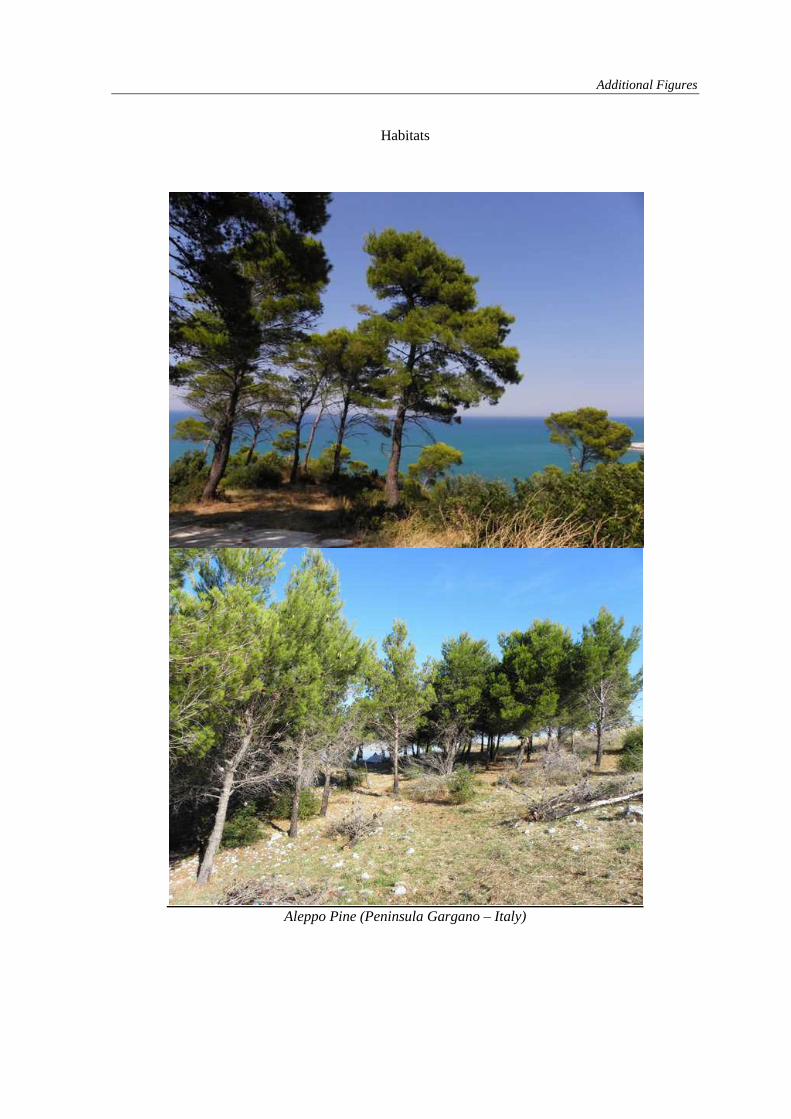
Additional Figures
Habitats
Aleppo Pine (Peninsula Gargano – Italy)

Additional Figures
European Black Pine, P. nigra subsp. nigra (NP Paklenica – Croatia)
European Black Pine, P. nigra subsp. laricio (NP Majella – Italy)

Additional Figures
European Black Pine, P. nigra subsp. dalmatica (Hvar – Croatia)
European Black Pine, P. nigra subsp. laricio (Aspromonte – Italy)
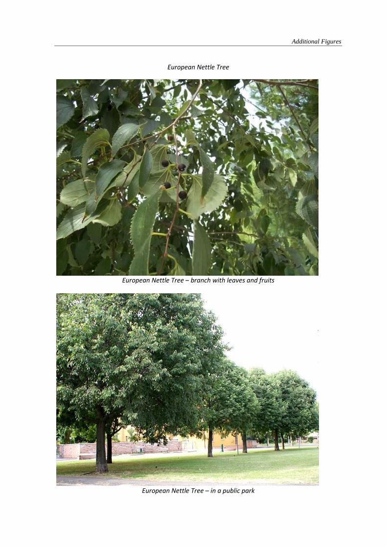
Additional Figures
European Nettle Tree
European Nettle Tree – branch with leaves and fruits
European Nettle Tree – in a public park

Additional Figures
Inula verbascifolia subsp. verbascifolia
Inula verbascifolia subsp. verbascifolia – in bloom
Inula verbascifolia subsp. verbascifolia – tipical habitat