soil spatial and temporal variability, assessment for site...

1

UNIVERSITA’ DEGLI STUDI DELLA TUSCIA

DIPARTIMENTO DI SCIENZE E TECNOLOGIE PER

L'AGRICOLTURA, LE FORESTE, LA NATURA E L'ENERGIA

Corso di Dottorato di Ricerca in

“Ingegneria dei Sistemi Agrari e Forestali”

XXVII Ciclo

Soil Spatial and Temporal Variability, Assessment for

site Specific Management

(s.s.d. AGR/09)

Tesi di Dottorato di:

Agr. Dott. Simone Bergonzoli

Coordinatore del corso: Tutor

Prof. Massimo Cecchini Dott.ssa Pieranna Servadio

Consiglio per la ricerca e la sperimentazione in agricoltura,

Unità di ricerca per l’ingegneria agraria

2

A chi non ci sta,

A chi veste i panni del guerriero,

To who thinks outside the box.

3

Acknowledgments

I would like to thank all persons that participate at field tests and made it possible

to perform the whole research.

I would like to thank particularly Dr. Pieranna Servadio for the fundamental help

in gathering and analysis of data and for the fundamental suggestions.

5

Abstract

The soil varies from place to place, and many of its properties vary in time too.

Within-field variation is the result of both spatial and temporal variation of biological,

edaphic, climatic, topographic and anthropogenic factors. There is a need in modern

agriculture of understanding spatial and temporal variability within fields.

The objective of this study was to analyze, to quantify and to assess the within

agricultural field spatial and temporal variability for site specific management.

Some soil physical-chemical parameters were investigated by means of

georeferenced samplings in order to study the variability of multiple soil variables and to

find soil indicators.

Performance of machineries during soil tillage and agricultural operations were

also investigated and analyzed with the aim of finding field efficiency indicators.

Geostatistical analyses were implemented to interpolate the acquired data and to

perform the cluster analysis.

The results of tests performed during the whole experimentation highlighted the

presence of high spatial variability of soil physical-chemical properties within the

agricultural fields examined.

Georeferenced sampling of soil physical-chemical parameters allowed to identify

soil quality and soil strength indicators, furthermore monitoring the performance of

machineries during soil tillage and agricultural operations allowed to identify field

efficiency indicators (i.e.: area specific consumption, global energy employed and fuel

energy requirements).

The assessing process of spatial variability within agricultural fields, the

identification of soil indicators and the definition of management zones can be

considered as an adaptation technique to Climate Change enhancing the efficiency of

agriculture. In fact, the defined management zones could provide information for site-

specific management, including the application of different soil tillage methods.

Furthermore, variable-rate application (VRA) instead of uniform-rate application

(URA) of inputs might be carried out, decreasing fertilization in the more productive area

and minimizing the application of chemical substances as a strategy to obtain a more cost-

effective field management.

7

INDEX

1. Introduction ....................................................................................... 7

2. Spatial variability of some soil properties and wheat yield within a trafficked field ........................................................................................ 7

2.1. Introduction .................................................................................... 7

2.2. Materials and methods .................................................................... 7

2.3. Results ............................................................................................. 7

2.4. Conclusion ...................................................................................... 7

3. Soil mapping to assess workability in Central Italy as climate change adaptation technique .............................................................................. 7

3.1. Introduction .................................................................................... 7


3.2.1. Sampling test and mapping ..................................................... 7

3.2.2. Soil tillage ................................................................................ 7

3.3. Results ............................................................................................. 7


3.3.1. Soil tillage and wheat yield ...................................................... 7

3.4. Conclusion ...................................................................................... 7

4. Soil workability and wheat yield in climate change scenarios ............. 7

4.1. Introduction .................................................................................... 7


4.2.1. Sampling test ........................................................................... 7

4.2.2. Soil tillage ................................................................................ 7

4.2.3.Statistical methods ................................................................... 7

4.3. Results ............................................................................................. 7

4.3.1. Sampling test ........................................................................... 7

8

4.3.2. Soil tillage ................................................................................ 8

4.4. Conclusion ...................................................................................... 8

5. Delineation of Site-Specific Management Zones in Wheat Field based on Soil Structural Stability, Shear Strength, Water Content, and Nitrogen 8

5.1. Introduction .................................................................................... 8


5.2.1. Site and data acquisition ......................................................... 8

5.2.2. Meteorological data ................................................................ 8

5.2.3. Sampling test, measurements, and mapping ........................... 8

5.2.4. Management zone identification ............................................. 8

5.3. Results and discussion ..................................................................... 8

5.3.1. Wheat yield ............................................................................ 8


5.3.3. Management zone identification ............................................. 8

5.3.4. Cluster analysis........................................................................ 8

6. Perspectives ........................................................................................ 8

7. Main conclusions ............................................................................... 8

8. References ......................................................................................... 8

9. Publications ........................................................................................ 8

10

1. Introduction The soil varies from place to place, and many of its properties vary in time too.

Within-field variation is the result of both spatial and temporal variation of biological,

edaphic, climatic, topographic and anthropogenic factors. Information about soil

variability is important in ecological modeling, environmental prediction, precision

agriculture, and natural resources management. With growing interests in precision

farming to address diverse environmental, ecological, agricultural, and natural resource

issues, an adequate understanding of soil variability as a function of space and time

becomes essential.

However, in spite of voluminous literature published in the past three decades or

so, knowledge about soil variability is still dispersed and requires further synthesis (e.g.,

Burrough, 1993; Heuvelink and Webster, 2001). In particular, there is a need to quantify

soil variability across multiple scales, which will undoubtfully enhance the use of soils

information in diverse applications.

Considerable work has been done investigating soil variability at a single scale,

which provides useful information at that particular scale (e.g., Beckett and Webster,

1971; Webster, 1985; Agbu and Olson, 1990; Gaston et al., 1990; Schellentrager and

Doolittle, 1991; Moore et al., 1993; Mahmoudjafari et al., 1997; Thompson et al., 1997;

Boehm and Anderson, 1997). However, quantification of soil variability at multiple scales

is often desirable for modeling and prediction, which provides a basis for developing an

understanding regarding scales of influence on variability and a framework upon which

scaling of data may be possible. Limited studies have been done so far to investigate soil

spatial variability across multiple scales (Burrough, 1983a, b; Edmonds et al., 1985;

Wösten et al., 1987; Pennock and de Jong, 1990; Sylla et al., 1996; Dobermann et al.,

1997).

Soil variability is influenced by different combinations of soil-forming factors

acting through space and time. In a general framework, soil variability may be considered

as a function of five space–time factors, i.e., spatial extent or area size, spatial resolution

or map scale, spatial location and physiographic region, specific soil property or process,

and time factor. Exact expression of such a function is very difficult, if not impossible, to

establish, in part because of the diversity and complexity of the relationships.

Variation within soil units is acknowledged, but described quantitatively in vague

terms. Soil surveys have traditionally overlooked spatial variability within map units for a

variety of reasons including scale limitations and inadequate quantitative data. Field

11

observations are made at a selected number of locations chosen by soil surveyors using

formal knowledge and intuitive judgment. Sampling the soil at a finite number of places

or points in time yields incomplete pictures; in fact soil surveys traditionally have lacked

appropriate sampling design to present quantitative estimates regarding spatial variability

within and across map units.

There is a need in modern agriculture of understanding spatial and temporal

variability within fields. Understanding such variation is essential for site-specific crop

management, which requires the delineation of management areas.

Traditionally, agricultural fields have been managed as single units, although it has

long been known that soil condition and crop yield are not homogeneous within them

(Frogbrook & Oliver, 2007; Vitharana et al., 2008; Alletto et al., 2010; López-Lozano et

al., 2010). In fact, variability of soil properties may affect crop growth, yield, and quality at

the within-field scale (Diacono et al., 2012). In this scenario, uniform field management

often results in over-application of inputs in areas with high nutrient levels, and under-

application of inputs in areas with low nutrient levels (Ferguson et al. 2003; Servadio et al.

2010). The magnitude and structure of such variability may suggest the suitability of site-

specific management, with the aim of increasing both profitability of crop production and

environment protection (Godwin & Miller, 2003; Mzuku et al., 2005; Vitharana et al.,

2006). Site-specific management can regulate production inputs and, consequently, can

reduce the risks and the negative impacts of pollution due to over-application of

chemicals (Di Fonzo et al., 2001; Basso et al., 2009; Basso et al., 2011). Moreover, the

enlargement of single management units, resulting from the enlargement of arable lands,

can encourage the application of non-uniform management techniques (Sylvester-Bradley

et al., 1999). The management zone (MZs) approach (Mulla et al. 1992) is a site-specific

management method, based on the determination of sub-regions characterized by

homogeneous combination of yield-limiting factors (Vrindts et al. 2005), generally

acknowledged as a possible way to address this problem (Cahn et al. 1994; McKinion et

al. 2001; Keller et al. 2012). The subdivision of the field in management zones (MZs) is

based on the knowledge of the spatial variability of soil parameters that are, generally,

stable with respect of time, and related to crop yield (Schepers et al., 2000; Schepers et

al., 2004). To delineate such zones, various parameters were evaluated in literature. For

example, MZs were defined considering yield (Vrindts et al., 2005; Xiang et al., 2007;

Diacono et al., 2012), soil fertility (Ortega & Santibáñez, 2007; Davatgar et al., 2012; Van

Meirvenne et al., 2013) or soil electrical properties (Morari et al., 2009; Moral et al.,

12

2010; Naderi-Boldaji et al., 2013; Doolittle & Brevik, 2014). A combined use of different

sets of parameters, such as a combination of physical and chemical soil parameters, could

lead to an in-depth investigation into spatial heterogeneity and to a more comprehensive

knowledge of soil plant system (Guastaferro et al., 2010; De Benedetto et al., 2013).

Among the physical parameters, soil strength influences many aspects of the cultivation,

such as performance of tillage and root growth. Furthermore, when compaction occurs,

soil permeability and regeneration can be reduced (Manuwa & Olaiya, 2012). Variations

of soil texture can also have a significant effect on soil management, as studied in previous

investigations (Vitharana et al., 2006; Gooley et al., 2014; Havaee et al., 2015). Once the

data set has been acquired, cluster analysis can be performed to define the management

areas (Taylor et al., 2003; Fleming et al., 2004), by implementing, for instance, fuzzy k-

means or Gustafson-Kessel algorithms (Höppner, 1999; Stafford et al., 1999; Vrindts et

al., 2005; Guo et al., 2013). The application of such analises allows taking into account

the continuous variation of natural soil variables (Burrough 1989) and it has been used to

identify potential within-field management zones in precision agriculture (Boydell and

McBratney 2002).

Cluster analysis or clustering is the task of grouping a set of objects in such a way

that objects in the same group (called a cluster) are more similar (in some sense or

another) to each other than to those in other groups (clusters). It is a main task of

exploratory data mining, and a common technique for statistical data analysis, used in

many fields. Cluster analysis groups similar multivariate data points into distinct classes in

the p-dimensional attribute space, defined by the p properties measured at each data

point within a field. The application of fuzzy set theory to clustering has enabled

researchers to account for the continuous variation in natural soil variables. It may be

more appropriate to consider any data point as having some similarities to more than one

cluster. Fuzzy classification determines the degree of resemblance of an object to a cluster

by its membership to the cluster. In practice, it may be necessary to assign each data point

to a unique class using the one of maximum membership, a process called

‘defuzzification’ (Guastaferro et al., 2010). The clustering procedure called fuzzy k-means

has been used to identify potential within-field management zones in precision agriculture

(Boydell and McBratney, 2002). Cluster analysis itself is not one specific algorithm, but

the general task to be solved. It can be achieved by various algorithms that differ

significantly in their notion of what constitutes a cluster and how to efficiently find them.

Popular notions of clusters include groups with small distances among the cluster

13

members, dense areas of the data space, intervals or particular statistical distributions.

Clustering can therefore be formulated as a multi-objective optimization problem. The

appropriate clustering algorithm and parameter settings (including values such as

the distance function to use, a density threshold or the number of expected clusters)

depend on the individual data set and intended use of the results. Cluster analysis as such

is not an automatic task, but an iterative process of knowledge discovery or interactive

multi-objective optimization that involves trial and failure. It will often be necessary to

modify data preprocessing and model parameters until the result achieves the desired

properties.

The management zone approach is based on the creation of areas (clusters) within

the agricultural field characterized by similar values of soil physical-chemical parameters.

Because such analysis is not modeled but based and influenced by the soil parameters

used for it, some problems arises in how and which parameters to select. For example

concerning texture in Vitharana et al., 2008 is reported to use as input parameter only

one fraction to avoid the spurious correlations due to the compositional nature of the

texture (individual elements sum to 100%). Some other properties show correlation

between each other such as for example soil strength parameters (cone index, shear

strength, bulk density) and water content, furthermore these are dynamic soil properties

that vary during the growing season but they are determined only once with soil

samplings.

Fuzzy k-means or Gustafson-Kessel algorithms are applied with original soil

variables as inputs that are selected by the users. Unconstrained classical k-means and

fuzzy k-means do not include spatial autocorrelation or any reference to the geographical

position of data points from which variables are recorded. A few attempts (Ping and

Dobermann, 2003; Frogbrook and Oliver, 2007; Milne et al., 2012) have been made to

spatially constrain the clustering algorithm to produce management zones, but these have

not been widely adopted.

Alternatively, a linear combinations of soil properties could be used to overcome

the problem in selection inputs variables of cluster analysis (Schepers et al., 2004; Li et

al., 2007; Xin-Zhong et al., 2009). Principal Component Analysis (PCA) (Hotelling, 1933)

has been used to build those linear combinations. Classical PCA is used to reduce the

number of original variables available for classification and to summarize the variability of

several variables in new synthetic variables. There are as many Principal Components as

variables included in the analysis. Generally, the first few components explain most of the

14

total variance in the data set and contain the main signal in the joint variability, instead the

last principal component is commonly associated with noise or spurious variability.

Usually only Principal Componens with eigenvalues ≥1 are selected for cluster analysis

and to develop the MZs as suggested by Jolliffe (1986).

The objective of this study was to analyze, to quantify and to assess the within

agricultural field spatial and temporal variability for site specific management.

Some soil physical-chemical parameters were investigated by means of

georeferenced samplings in order to study the variability of multiple soil variables and to

find soil indicators.

Performance of machineries during soil tillage and agricultural operations were

also investigated and analyzed with the aim of finding field efficiency indicators.

Geostatistical analyses were implemented to interpolate the acquired data and to

perform the cluster analysis. The geostatistical analyses were conducted using the FuzMe,

MatLab and the Geostatistical Analyst extensions of the ArcGIS 10.0 software (Esri Inc.,

Redlands, CA, USA) that was used also for graphical representation.

Case studies were analysed and field tests were established, and results are

reported as follows.

15

2. Spatial variability of some soil properties and wheat yield within a trafficked field

2.1. Introduction All soil properties are susceptible to vary with time and space as a consequence of

land use, water content level and management system adopted. The implementation of

intensive agricultural production systems has led to the use of heavy machines with high

working capacity requiring high traction forces. Repeated passes on the field can cause

soil compaction creating pans, having a low permeability to water and nutrients and a high

resistance to root penetration (Servadio, 2010). The intensity and distribution of the

traffic of agricultural machines may cause a high spatial variability of soil physical

properties and yield, even in soils characterised by spatial homogeneity of physical

properties (Mouazen et al., 2001; Carrara et al., 2007). Consequently, uniform

management of fields often results in over-application of inputs in areas with high nutrient

levels and under-application in areas with low nutrient levels (Ferguson et al., 2003;

Servadio et al., 2010). Site-specific management has been acknowledged as one means of

addressing this problem (Cahn et al., 1994; McKinion et al., 2001). The most popular

approach for managing spatial variability within fields is the use of management zones

(MZs) (Mulla et al., 1992), which are field subdivisions that have relatively homogeneous

attributes in yield and soil condition.

The objectives of this study were: (1) to investigate the spatial variability of some

soil properties and crop yield, within a trafficked field just after two fertilizing operations,

to evaluate whether these soil properties could be used as indicators of crop yield; (2) to

develop statistical correlations among the measured soil parameters and yield and (3) to

represent the spatial variability within the field using georeferenced maps as basis for zone

management.

2.2. Materials and methods Field tests were carried out in a farm near Rome (41°52’502’’ Latitude (N);

12°12’866” Longitude (E) on a clay soil classified as Vertic Cambisol (FAO, 1998). The

soil was previously tilled with a cultivator at 0.40 m depth, harrowed at 0.20 m depth with

a rotary harrow in October and afterwards was sown with wheat.

16

The fertilizations were carried out in March and in April using the following

machines respectively:

1) a wheeled tractor (73.5 kW engine power) equipped with extra large and low aspect

ratio tyres (4620 kg mass, front and rear tyres inflation pressures were 70 and 60 kPa

respectively) and its trailed broadcaster, for a total of four axles (1520 kg mass + 1200 kg

fertilizer with an operative width of work of 14 m; front and rear tyre inflation pressures

were 60 and 70 kPa respectively) coded WTEL;

2) a self propelled broadcaster (sprayer) (130 kW engine power) fitted with isodiametric-

narrow tyres (11700 kg mass with front ballast + 2500 kg fertilizer tank with an operative

width of work of 24 m; front and rear tyres inflation pressures were 290 kPa) coded

WTN.

During the wheat fertilizing, a DGPS receiver was placed on the tractors to

monitor passes across the whole field and saving position data. The total track area

covered by the machine tyres during the fertilization were calculated with help of the

software ArcGis 10 (Kroulik et al., 2009). In April, on the whole field, a 60-m grid

sampling of 20 samples of soil was performed to determine physical-chemical properties:

particle size, water content, total nitrogen (N) and organic matter (OM) and 20

penetration resistance were measured from 0 to 0.20 m depth both taking the GPS

position to produce interpolated maps describing spatial variability. Penetration resistance

of the soil (CI) was measured using a penetrologger with GPS (Eijkelkamp). Total soil N

was measured by the Kjeldahl method; total organic carbon (C) with the wet oxidation

(Walkley and Black 1934). Soil water content at the time of field tests was 33.2 g (100 g)-1

(over field capacity), it was measured from 0 to 0.20 m depth. Field capacity, determined

by pressure plate extractor was 28 g (100 g)-1.

At the end of the crop cycle, during the wheat harvesting, a grain yield map was

acquired with a combine harvester, equipped with grain mass flow sensor, GPS and

Precision Land Management Software that was used to read out the yield data.

Interpolation of soil properties and grain yield maps was performed using the

software ArcGIS and the spatial analyst tool natural neighbor (Servadio and Blasi, 2003;

Servadio et al., 2011). To develop correlations, twenty yield values were taken from the

grain yield map using the same georeferenced grid sampling corresponding to the soil

samples.

17

2.3. Results From the analysis of penetration resistance (Fig. 1) and water content (Fig. 2)

maps, it emerged the presence of homogeneous and well defined areas that highlighted

the spatial variability within the field. Areas characterized by high values of soil water

content ranging between 33 up to 45 g 100g-1, over field capacity, and high degree soil

strength, due to the different intensity of the traffic of agricultural machineries were

found.

Figure 1(Left). View of field map of penetration resistance (MPa)(0-0.20 m depth) Figure 2 (Right). View of field map of water content (g 100g-1). ( Sampling locations)

Spatial variability within field was highlighted also by soil chemical parameters

maps. From the analysis of the results of Table 1 and of the maps it emerges high value of

CV and the presence of homogeneous and well defined areas that highlight the spatial

variability within the field.

Table 1. Mean value [g(100 g)-1] and CV (%) of soil physical-chemical parameters

Properties Mean value a g (100 g)-1 CV (%)

Sand (2000-50 mm) 20.3 85.0

Clay (<2 mm) 53.0 20.1

Silt (50-2 mm) 26.7 30.7

Water content 33.2 7.58

Organic matter 2.5 16.3

Nitrogen 0.20 19.2

Cone index 0.64 MPa 15.6

18

Properties Mean value a g (100 g)-1 CV (%)

Yield

4.52 t/ha 28.5

Grain yield (Fig. 3) also shows spatial variability with high, mean and low yielding

zones. In fact, significant correlations found between soil nitrogen and yield and between

soil organic matter and yield confirmed that in agricultural ecosystems, N and OM are the

major determinants and indicators of soil fertility and quality, which are closely related to

soil productivity.

Figure 3. View of yield map

The results obtained show that agricultural management can affect the spatial

patterns of soil properties that are spatially correlated. Geo-referenced measurements and

interpolated maps are needed to describe the spatial variation of soil parameters and crop

yield. Field maps would provide the basis of information for rationally managing soil

nutrients and soil tillage. In fact, spatial variability within field suggested that variable rate

fertilization application and variable depth tillage may be helpful to maximize

environmental benefits and to improve quality of the crop and to reduce soil compaction.

Kind and intensity of soil tillage can be adapted at the different zones and variable

depth tillage could be applied working only on the compacted area. According to Vrindts

et al (2004), Keller et al (2010), Servadio et al (2011), each management zone gets the

appropriate level of inputs and is usually defined on the basis of soil and yield

information. Therefore fuel, labour, equipment wear and tear and environmental costs

could be reduced.

19

2.4. Conclusion To traffic the soil during fertilization, carried out with high soil water content, the

use of a tractor fitted with extra large tyres was necessary. With lower soil water content,

the use of narrow tires allowed carrying out fertilization avoiding excessive crop trampling

and covering smaller (more compacted) field area with respect to a tractor equipped with

extra large tyres.

The within-field spatial variability of soil properties and crop yield was highlighted

both from the high values of CV and from the presence of homogeneous and well

defined areas found in the fields maps.

Obtained correlations between soil properties (OM and N) and yield confirmed

that in agricultural ecosystems, N and OM are the major determinants and indicators of

soil fertility and quality, which are closely related to soil productivity.

Spatial variability of field maps highlighted that management zone could be

applied for rationally managing soil tillage and fertilizing operations.

20

3. Soil mapping to assess workability in Central Italy as climate change adaptation technique

3.1. Introduction Soil tillage represents the most influential manipulation of soil physical properties

because of repetitive application, its depth range extending up to tens of centimeter and

because it influences the type of residue management applied. The need of sustainable

agriculture and the increased cost of fuel in tillage operations forced farmers to change

the farming methods (Yalcin and Cakir, 2006). In fact, many studies have been done to

compare tillage practices, particularly tillage versus no-tillage (NT). Conventional tillage

may accelerate mineralization of organic matter, reduce soil fertility, increase water

consumption, and deteriorate chemical and physical properties of soil (Chen et al., 2007).

On the contrary minimum-tillage and no-tillage, characterized by minimal soil

disturbance (Paremelee et al., 1990), may be a good choice for land preparation because

it has potential benefits including reduced production costs, saving in fuel, equipment and

labor (Allmaras and Dowdy, 1985) as well as soil conservation (Uri, 1997), furthermore

direct seeding may be an efficient technology to replace transplanting because it is simple

and labor-saving (Wu et al., 2005). Improvements in the design of minimum and no-till

drills, lower cost and more effective herbicides, a better understanding of the role of

tillage in crop production systems, and an increased emphasis on residue management

have been key factors in the successful shift to direct seeding (Fowler, 1995), that have

slowly become an accepted alternative to conventional tillage systems (Collins and Fowler,

1996). According to Yalcin and Cakir (2006) no-tillage seems to result one of the most

sustainable soil management systems, because it reduces labour requirements and

machinery costs, fossil-fuel inputs, and soil erosion, while it increases available plant

nutrients, soil organic matter content, soil quality, and improves the global environment.

The major sources of GHG fluxes associated with crop production are soil N2O

emissions, soil CO2 and methane (CH4) fluxes, and CO2 emission associated with

agricultural inputs and farm equipment operation (Adler et al., 2007). Loss of soil organic

carbon (SOC) under conventional tillage have been extensively documented (West and

Post, 2002; Conant et al., 2007), on the contrary conservation tillage practices (minimum

and no tillage) may play a leading role in sequestering CO2 achieving a mitigation effect of

CC. In fact NT farming is recommended to conserve soil and water but its potential to

sequester SOC varies widely due to complex interactions among climate, soil type, crop

21

rotation, duration and management factors (Vanden Bygaart et al., 2002; Puget and Lal,

2005). Long-term (>10 yr) of NT practices have also the potential to reduce greenhouse

gas emissions in humid climates (Chatterjee and Lal, 2009).

The objectives of this study were: 1) to investigate spatial variability of soil

properties, to found soil quality indicators and to asses soil workability 2) to investigate the

machine performance, the fossil-fuel energy requirements and the CO2 emissions from

agricultural machinery in summer soil tillage operations both on hilly and plain field

carried out at very low water content, compared with direct-seeding.

3.2. Materials and methods

The study was conducted in Central Italy in two adjacent on-farm sites on a hilly

(178 m.a.s.l.), (43°33’17.181” N, 13°03’59.684” E) and on a plain fields (119 m.a.s.l.),

(43°33’21.664” N, 13°04’12.49” E) on a silty clay soil seeded with common wheat

(Triticum aestivum).

3.2.1. Sampling test and mapping

In order to assess the soil workability, two adiacent on-farm sites, an hilly (1.1 ha)

and a plain field (1 ha) were selected for field tests. Geo-referenced sampling tests based

on a grid of 50 x 50 m for each field were carried out investigating some soil physical

properties from 0 to 0.20 m depth. To produce interpolated maps and to describe spatial

variability of soil properties the software ArcGIS and the spatial analyst tool natural

neighbor (Servadio et al., 2011; Servadio and Bergonzoli, 2013) were used. Detected

physical-mechanical soil parameters were: particle size distribution, shear strength (SS),

dry bulk density (DBd), water content (WC), field capacity (Fc) and structural stability of

soil aggregates (Sssa). Soil shear strength was measured using a field inspection vane tester

from 0 to 260 kPa (Eijkelkamp). In each field ten shear strength readings were taken in

increments of 0.05 m to a depth of 0.20 m. Dry bulk density was measured by taking ten

samples of soil using a corer sampling ring of 100 cm3 of volume at 0-0.20 m depth. Soil

water content at the time of field tests was measured from 0 to 0.20 m depth by taking

samples of soil that were weighed and dried until they reached a constant weight. Soil

field capacity was determined using the pressure plate extractor.Structural stability of soil

aggregates was determined on the 0.25 mm fraction through the method of Kemper

(1965).

22

Total organic carbon (C) was determined with the wet oxidation method (Walkley

and Black, 1934), organic matter content (OM) was derived from the total organic carbon

(C x 1.72) and cation exchange capacity (CEC) by the barium chloride (BaCl2)–

triethanolamine (TEA) method. Exchangeable bases [sodium (Na)], was determined

using 1 M ammonium acetate (NH4OAc) solution (soil/solution ratio 1:10, shaking time

30 min), available phosphate (P2O5) was determined with the Olsen method, colloid index

(Ci), a parameter used to evaluate colloid behavior, was calculated as follows:

Ci = 10 X1 + X2

Where: X1 is organic-matter content (%) and X2 is clay content (%), (Beni et al., 2012).

During the overall experimentation time, (2011 and 2012), meteorological data (monthly

rainfall, minimum and maximum temperatures) were also recorded.

3.2.2. Soil tillage

Conventional soil tillage was carried out in July 2011 both on hilly and plain fields

on Silty Clay soil at very low water content (0.25 and 0.31 of the field capacity

respectively), in addition direct-seeding + fertilizing was carried out in plain field in

September 2011 at 0.25 of the field capacity. Same field conditions during the tests are

shown in Table 2.

Plowing was carried out with the following work sites layout: 1) a very high power

wheeled tractor (217 kW engine power; 9684 kg mass + 1600 kg front ballast) with

reversible semi-mounted four furrow plow (2300 kg mass) operating on hilly field (WT-

hilly). 2) a mean power metal tracked tractor (120 kW engine power; 14000 kg mass) with

trailed three furrow plow (1100 kg mass), operating on plain field (TT-plain).

Soil tillage operations were performed at very low water content, 9.8 % and 11.6

% for treatments WT and TT respectively.

Direct seeding was carried out by means of a very high power wheeled tractor

(265 kW engine power; 18000 kg mass) with hydro-mechanical power transmission with

trailed grain drill, a seeding unit, which consists of a seed and fertilizer box mounted

above two rows of opener assemblies (for a total of 16 no till opener) operating on plain

field (GD+F-plain). The front of the unit is supported by the tractor hitch, the back of the

unit is supported by two wheels. Direct seeding was performed at 9 % water content.

23

The performance of the tractors and machineries during tillage operations were

quantified through the following parameters: forward speed, tractors slip (%), effective

work capacity (ha h-1), measured work width (m), work depth (m), soil rise and roughness

(m), clod size distribution (%), energy power output (kW), hourly (kg h-1), global energy

employed (kWh ha-1), fossil-fuel energy requirements (GJ/ha) and carbon dioxide

emissions (kg C ha-1) (Servadio and Bergonzoli, 2012; Marsili and Servadio, 1998). In

addition field data collected has allowed to appraise the global energetic efficiency of the

tractors that depends from the area (ha) covered in function of the time and from the

ability of the tractor to convert the energy of combustion in useful power. As a result, two

field oriented performance indicators consisting in time efficiency (h ha-1) and area

specific consumption (kg ha-1) are applied (Burgun et al., 2013).

3.3. Results 3.3.1. Sampling test and mapping

Results of the sampling tests of the soil properties are shown in Table 2 and in

Figs. 4. Results of Table 2 show, both on plain and hilly fields, very high values of shear

strength (over 180 kPa) and its CV% and high values of dry bulk density (over 1.39 Mg m-

3). Values of structural stability of soil aggregates were higher on hilly field (56%) with

respect to the plain (31.5%). Higher values of organic matter (1.54 %), P (11.5 ppm) and

Na (3.10%) were found on plain field.

Table 2. Mean values (0-0.20 m depth) and coefficient of variation of some soil chemical-physical properties (June 2011)

Soil properties Plain Hilly

Meana CV (%) Meana CV (%)

Sand (g/100g)b 9.25 25 8.06 27.8

Silt (g/100g)b 43.1 6.35 41.6 5.63

Clay (g/100g)b 47.6 5.47 50.3 6.76

Textureb Silty Clay

Shear strength (kPa) 188 33.8 222 41.4

Dry bulk density (Mg m-3) 1.39 9.79 1.48 8.50

Water content (%) 31.2 9.69 29.1 11.7

Structural stability of soil aggregates(%)

31.5 - 56 -

24

Soil properties Plain Hilly

Field capacity (%) 36.7 - 37.9 -

OM (%) 1.54 14.8 1.30 14.9

TOC (%) 0.89 14.8 0.75 14.9

P (ppm) 11.5 13.2 5.87 36.7

CEC (meq %) 27.5 4.50 27.2 4.21

Na (%) 3.10 47.6 1.92 34.6 a Average of ten values, bUSDA classification; OM, organic matter; TOC, total organic carbon; CEC, cation exchange capacity. Figures 4 a, b, c and d. Results of the interpolation of soil properties maps performed by using the software ArcGIS and the spatial analyst tool natural neighbour.

a

b

25

c

d

Figure 4. View of field maps of soil parameters studied: a) organic matter (%); b) shear strength (kPa); c) dry bulk density (Mg m-3); d) water content (g/100g)

From the analysis of OM (Fig. 1a), SS (Fig. 1b) and DBD (Fig. 1c) interpolated

maps it emerged the presence of an homogeneous and well defined zone in the eastern

part of the plain field characterized by low level of soil strength (SS < 80 kPa and DBD

<1.38 Mg m-3) and high organic matter content (OM>1.55%). Therefore this area was

assessed to perform the direct seeding of common wheat. The analyzed soil parameters

can be considered good indicators of the soil strength and according to the soil water

content, useful to assess workability.

3.3.1. Soil tillage and wheat yield Results of machineries performance during plowing and direct-seeding are shown

in Table 3.

During CT operations carried out at 0.40 m work depth, both work sites layout

showed good traction performance indicated from slip values always lower than 15%

26

(Table 2). This result, besides to the low soil water content and high soil strength, were

also due to the high contact area of the tracks on soil of TT-plain and to the high engine

power of WT-hilly (Servadio, 2010). For wheeled tractor, hourly fuel consumption was

higher (47 kg h-1) with respect to the tracked tractor (27 kg h-1); time efficiency of WT-hilly

was enhanced from the larger work width 1.07 h ha-1 with respect to the 1.78 h ha-1 of the

TT-plain; furthermore area specific consumption was of similar magnitude (48-50 kg ha-1).

According with Burgun et al., (2013), this prove that the use of the wide

implements enhance the time efficiency and simultaneously reduce the area specific

consumption more than to use of higher forward speed. Regarding the grain-

drill+fertilizing operating in plain area, due to the high forward speed and work width,

time efficiency resulted 0.26 h ha-1 and area specific consumption resulted 11 kg ha-1.

Table 3. Performances of work sites layout during ploughing (July 2011) and direct-seeding (September 2011) and yield (June 2012)

Work site layout

TT-plain WT-hilly GD+F-plain

Forward speed (m s-1) 1.25 1.21 3.5

Mean rise (m) 0.20 0.30 -

Mean roughness (m) 0.22 0.31 -

Measured work width (m) 1.25 2.13 3.0

Measured work depth (m) 0.40 0.40 0.03

Effective work capacity (ha h-1) 0.56 0.93 3.8

Time efficiency (h ha-1) 1.78 1.07 0.26

Reliefs on the tractors

Slip (%) 14.1 6.93 -

Energy power output (kW) 120 217 200

Fuel consumption

Hourly (kg h-1) 27 47 40

Specific (g kWh-1) 225 220 210

Area specific consumption (kg ha-1) 48 50 11

Global energy employed (kWh ha-1) 214 232 52

Energy (GJ ha-1) 2.24 2.35 0.52

CO2 emission (kg C ha-1) 47.6 50.0 11.0

27

Despite to the higher energy power output of the very high power wheeled tractor

(WT-hilly), global energy employed were of similar magnitude of the mean power metal

tracked tractor (TT-plain) because of the good time efficiency. Global energy employed

was of only 52 kWh ha-1 for direct-seeding. According to Yalcin and Cakir (2006),

conventional tillage method had the higher fuel consumption and the lower field

efficiency as compared to the direct seeding. Fossil-fuel energy requirements from the two

tractors used during plowing were of similar magnitude, in fact it was 2.24-2.35 GJ ha-1

during conventional tillage while it was significantly lower (0.52 GJ ha-1) during direct-

seeding. Carbon dioxide emissions were of similar magnitude during plowing, it was 47.6-

50.0 kg C ha-1 during conventional tillage while it was significantly lower (11.0 kg C ha-1)

during direct-seeding.

Yield results of wheat (Table 4) can be ascribed to the climatic trend. The

monthly mean temperature and rainfall recorded during the growing season (2011-2012)

shown the maximum temperature values higher than 10 °C during phase of culm growth.

Furthermore the rainfall distribution from February to May ensured water

requirements of the crop during the phases of culm growth and physiological maturity.

Trends of precipitation and temperatures allowed a good development of the crop that

did not undergo stress and recorded yield value similar to the crop under conventional

tillage management. In fact wheat yield of direct seeded field resulted of similar

magnitude (only 9% lower) than that recorded on fields under conventional tillage.

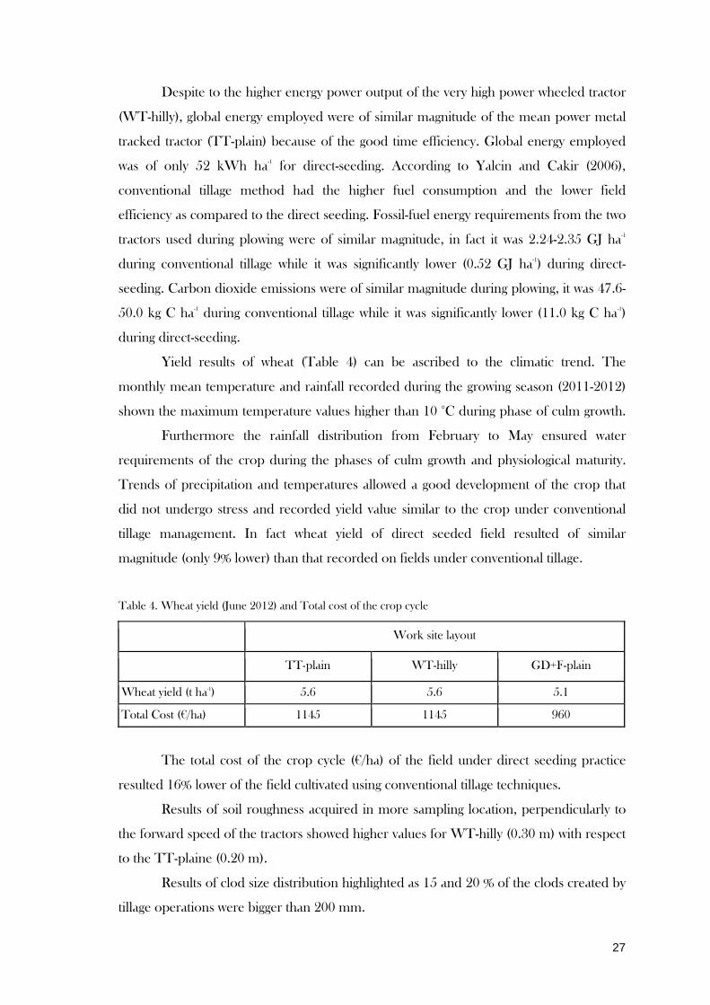
Table 4. Wheat yield (June 2012) and Total cost of the crop cycle

Work site layout

TT-plain WT-hilly GD+F-plain

Wheat yield (t ha-1) 5.6 5.6 5.1

Total Cost (€/ha) 1145 1145 960

The total cost of the crop cycle (€/ha) of the field under direct seeding practice

resulted 16% lower of the field cultivated using conventional tillage techniques.

Results of soil roughness acquired in more sampling location, perpendicularly to

the forward speed of the tractors showed higher values for WT-hilly (0.30 m) with respect

to the TT-plaine (0.20 m).

Results of clod size distribution highlighted as 15 and 20 % of the clods created by

tillage operations were bigger than 200 mm.

28

Therefore the degree of crushing of the soil required further operation to seedbed

preparation. Using a wheeled tractor of 167 kW, p.t.o. power with mounted rotary

harrow having 6.0 m work width and 0.74 m s-1 forward speed, time efficiency was 0.62 h

ha-1 area specific consumption was 22 kg ha-1, global energy employed was 97 kWh ha-1

Energy was 1.04 GJ ha-1 and CO2 emission was 22 kg C ha-1. All these parameters must be

added to the TT-plain and WT-hilly treatments.

3.4. Conclusion

As the field sampling and mapping have allowed more efficient resource

management, the use of precision agricultural practices and information technologies (IT)

have enhanced our understanding and the possibility to predict temporal and spatial

variability of soil properties in response to management practices. For instance, some

indicators of soil compaction/strength as SS, BD and OM were found and an area to

perform direct seeded was selected. During CT, good traction performance, with slip

values always lower than 15%, were found. Area specific consumption, global energy

employed and fuel energy requirements were significantly higher during CT operation

compared to direct seeding. Consequently, carbon dioxide emissions from different

agricultural machineries were lower during direct-seeding. Due to the favorable climatic

trend during the wheat growing season, the wheat yield of direct seeded field was of

similar magnitude (only 9% lower) of that recorded on fields under conventional tillage;

the total cost of the crop cycle (€/ha) was 16% lower compared to the field cultivated

under CT techniques. In conclusion, with the use of IT, hydro-mechanical power

transmission and the direct seeding technique, saving in energy and in CO2 emission can

be achieved and can be considered as good Climate change adaptation techniques.

29

4. Soil workability and wheat yield in climate change scenarios 4.1. Introduction The number of days available for field work is frequently central, either directly or

indirectly, to farm planning decisions. The number, and distribution, of working days

influences the type and acreage of crops grown, and the corresponding labour and

machinery requirements. The condition of land for field operations can be classified in

terms of trafficability and workability. Trafficability is concerned with the ability of soil to

provide adequate traction for vehicles, and withstand traffic without excess compaction or

structural damage. If land is considered trafficable, then it is deemed suitable for non-soil-

engaging operations (e.g. fertilizer application and crop protection). Workability is

concerned with soil-engaging operations and can be considered to be a combination of

trafficability and the ability of soil to be manipulated in a desired way without causing

significant damage or compaction. The most influential factor in determining the

suitability of land for field operations is the soil moisture status. When a soil is trafficked

or worked when in an unsuitable condition, damage to the soil's structure and the

consequent effect on crop production can persist for many years (Earl, 1997). In

mechanised agriculture, high axle loads cause major concern regarding the risk of soil

compaction, especially if wheeling and tillage are conducted at high soil moisture content

(Koch et al., 2008). Tillage is a fundamental factor influencing soil quality, crop

performance and the sustainability of cropping systems (Munkholm et al., 2012) because

represents the most influential manipulation or alteration of soil physical properties due

to repetitive application, its depth range extending up to tens of centimeter, and because it

influences the type of residue management applied (Mark et al., 2008).

Soil penetration resistance measurements have been effectively used in many

studies as a tool for characterizing soil strength after tillage (Utset and Cid, 2001).

However, soil penetration resistance as well as other soil property is affected by the soil

spatial variability and has been shown to strongly depend on soil water content (Becher,

1998; Servadio, 2010; Servadio 2013). Therefore the spatial and temporal variability of

soil compaction should be affected by soil moisture. Lyles and Woodruff (1962) found

that soil moisture content during tillage affected the size distribution of aggregates

produced and that aggregates formed at low moisture content had three to four times

more resistance to crushing than those formed at greater moisture contents. The type of

tillage implement also affects the soil structure produced. Tillage implements vary in

30

terms of both width and depth and in terms of the intensity in soil overturn administered

by the implement design (disc versus ploughing, etc.). Furthermore, interactions between

natural factors (e.g., soil type, climate and weather) and crop selection determine the

intensity, depth, frequency, and timing of tillage (Strudley et al. 2008) which highlights the

need for understanding the tillage effects on soil properties, tractor performance and crop

yield (Servadio and Bergonzoli, 2012a; Servadio and Bergonzoli, 2012b). Tillage systems

are location specific, so the degree of their success depends on soil, climate, and

management practices (Hajabbasi and Hemmat, 2000; Servadio et al., 2014).

The objectives of this study were to assess which tillage techniques could be

considered as adaptation in CCS. For this, the effects of three different main preparatory

tillage operations of wheat: ploughing at 0.4 m and 0.2 m depth and minimum tillage

(harrowing at 0.20 m depth), each of them carried out at two different soil water contents

(58% and 80% of field capacity) were compared and quantified. The quality of the

different tillage operations were assessed through wheat yield, clods size, soil water

infiltration, structural stability, cone index, shear strength.

4.2. Materials and methods The study was conducted in Central Italy on a hilly plateau (57 m.a.s.l.), (42°05’57.84” N,

12°38’09.59” E) on a silt loam soil seeded with wheat (Triticum durum variety Duilio).

Table 5. Soil conditions during field tests (0-0.20 m depth).

Particle size distribution (%): Sand (2000 - 50 mm) 24.7

Silt (50 - 2 mm) 52.5

Clay (< 2 mm) 22.7

Texture Silty loam

pH 6.4

Organic matter (%) 2.4

Field capacity (%) 31

Moisture content (%) measured during:

Sampling tests carried out on 20.10.2010 (LH) 18

Soil tillage carried out on 21.10.2010 (LH) 18

Soil tillage carried out on 15.11.2010 (HH) 25

Sampling tests carried out on 15.02.2011 (HH) 22

Three tillage treatments were compared: Minimum tillage, (harrowing 0.20 m

depth) coded MT; Ploughing, superficial (0.2 m depth) coded P20 and deeper (0.4 m

depth) coded P40. All treatments were carried out at two different soil conditions: high

31

water content (25%, treatments HH), corresponding to 80% of field capacity and low

water content (18%, treatments LH), corresponding to 58% of field capacity. The main

factor was the soil tillage, (MT, P20 and P40), while the secondary factor was soil water

content (LH and HH). The six treatments: P40 LH, P40 HH, P20 LH, P20 HH, MT

LH, MT HH, were arranged according to the split plot design; divided in three blocks of

six plots and replicated three times for a total of eighteen plots each of 200 m2.

4.2.1. Sampling test Two sampling tests of these soil properties were carried out: one on 20 October

2010, with water content at 58% of field capacity, to assess soil physical conditions before

starting the trials; another, on 15 February 2011, with water content at 78% of field

capacity, to evaluate and compare the strength of the soil after the tillage (Tab. 5). The

Richards water extraction apparatus was used to determine soil field capacity. Every

parameter detected into the experimental site was georeferenced.

4.2.2. Soil tillage Soil tillage was carried out at two different moisture content: in October at low

water content (58% of field capacity) and in November at high water content (80% of field

capacity). Same field conditions during the tests are shown in Table 5.

Ploughing was carried out using: 1) a mean power wheeled tractor (62 kW engine

power, 3400 kg mass front ballasted) with mounted one furrow plow while minimum

tillage was carried out using a mean power metal tracked tractor (62 kW engine power,

4100 kg mass front ballasted) with trailed disk harrow.

The performance of tractors carrying out tillage operations were evaluated

through: forward speed, slip, global energy employed, effective work capacity, real work

width and work depth, fossil-fuel energy requirements (GJ/ha) and carbon dioxide

emissions (kg C/ha). In addition field data collected has allowed to appraise the global

energetic efficiency of the tractors that depends from the area (ha) covered in function of

the time and from the ability of the tractor to convert the energy of combustion in useful

power. As a result, two field oriented performance indicators consisting in time efficiency

(h/ha) and area specific consumption (kg ha-1) were applied (Burgun et al., 2013; Servadio

et al., 2014).

In order to evaluate the quality of the tillage operations, the followings parameters

32

were measured: clod size distribution was determined by taking samples of tilled soil,

sifting them through sieves with holes of 200, 100, 50, 25 and 10 mm of diameter and

then separating into size classes (Servadio et al., 2012a and 2012b); structural stability of

soil aggregates on the 0.25 mm fraction through the method of Kemper (1965). Besides,

the wheat harvesting was carried out by hand into the sampling areas consisting in 1 m2

(for 6 replications), sampling areas were chosen trough a subjective method suggested by

Barbour (1998).

4.2.3.Statistical methods Statistical analyses of differences between treatments were made with analysis of

variance by means of the student’s test conducted, at different depth between the same

treatment and at the same depth between different treatments. Mean results are flanked

on the same line by letters. Each mean, which share a letter, does not differ significantly,

level of significance 0.01 (Gomez and Gomez, 1976).

4.3. Results 4.3.1. Sampling test In recent years, the weather conditions in Central Italy have been unstable. In

summer time soil was very dry and strength, in autumn and spring time soil was too mach

wet and the rainfall has generally been delayed until November-December. Hence,

farmers did not accomplish the seedbed preparation at the proper time. As a result, the

drilling of cereals such as wheat and barley has been so delayed that there has been a

decrease in yield. Meteorological data (rainfall) and the monthly mean rainfall during the

overall experimentation time were also recorded. During the sampling tests carried out

before tillage, with a soil water content corresponding to 58% of the field capacity (case

B), soil was very strength. In fact, the values of penetration resistance in the deeper layer

and of shear strength (Tab. 6 and 7) were very elevated with CI up to 4 MPa and SS up to

189 kPa. Due, both to the de-compacting action of soil tillage and to the higher water

content (71% of field capacity), these values decreased significantly (�>50%) in the

sampling tests carried out after tillage (case A).

33

Table 6. Mean values of soil layers from 0 to 0.40 m depth of penetration resistance carried out before (case B) and after (case A) tillage and its increment ratio ∆.

Treatments Depth (m) Mean Penetration Resistancea (MPa) (21.10.2010) (B)

Mean Penetration Resistancea (MPa) (15.02.2011) (A)

MT LH 0.0-0.20 2.77 a 1.34 b 0.52

0.21-0.40 4.36 b 1.91 a 0.56 P20 LH 0.0-0.20 2.53 c 0.91 e 0.64

0.21-0.40 3.99 e 1.55 f 0.61 P40 LH 0.0-0.20 2.19 d 0.92 e 0.58

0.21-0.40 3.89 e 1.30 f 0.66 MT HH 0.0-0.20 2.48 a 1.32 b 0.47

0.21-0.40 4.41 b 1.91 a 0.57 P20 HH 0.0-0.20 2.42 ac 1.26 a 0.48

0.21-0.40 3.75 d 1.83 b 0.51 P40 HH 0.0-0.20 2.78 a 0.96 e 0.65

0.21-0.40 3.96 de 1.31 f 0.67 a Average of 240 values.

Table 7. Mean values from 0 to 0.20 m depth of shear strength carried out before (case B) and after (case A) plough and its increment ratio ∆ Treatments Depth (m)

Mean shear strength a (kPa) (21.10.2010) (B)

Mean shear strength a (kPa) (15.02.2011) (A)

MT LH 0.0-0.20 172.83 a,b 83.83 a 0.51

P20 LH 0.0-0.20 155.67 a 42.33 b 0.72 P40 LH 0.0-0.20 188.67 b 56.50 bc 0.70 MT HH 0.0-0.20 154.50 a 72.75 ab 0.52 P20 HH 0.0-0.20 165.33 a 45.42 b 0.72 P40 H 0.0-0.20

177.50 a 37.67 b 0.78 a Average of 18 values.

4.3.2. Soil tillage Due to the high soil strength in term of CI and SS obtained in the tests carried out

at low water content, the tractor performance during ploughing was not so good if

compared with that of other studies carried out, for instance, on silty clay soil (water

content at 0.25 of the field capacity) with 217 kW powered wheeled tractors (Servadio et

al., 2014). In fact, the two field oriented performance indicators consisting in time

efficiency (h/ha) and area specific consumption (kg ha-1) applied, showed:

1) in the tests carried out at water content of 58% of the field capacity, the results

of the time efficiency were very low (8 and 6.3 h ha-1) for 0.40 and 0.20 m respectively

34

(Tab. 8). Accordingly, the results of area specific consumption for 0.40 and 0.20 m

respectively were 120 and 91 kg ha-1, fossil-fuel energy requirements (4.67 and 3.54 GJ ha-

1) and CO2 emission (101 and 77 kg C ha-1) were very high. Besides, tractor slip were very

high (32.4%), particularly during ploughing at 0.40 m depth.

2) in the tests carried out at high water content (80% of the field capacity), the

results were significantly best: the time efficiency were (6 and 4 h ha-1) for 0.40 and 0.20 m

respectively (Tab. 9). Accordingly, the results for 0.40 and 0.20 m depth were: area

specific consumption 91 and 60 kg ha-1, fossil-fuel energy requirements 3.54 and 2.33 GJ

ha-1 and CO2 emission 77 and 51 kg C ha-1 respectively. Tractor slip (16 and 17%) can be

considered as good for a wheeled tractor during plough. Tractor slip is an index of

traction performance and to obtain the maximum of the traction efficiency, slip mast be

from 15 to 20% on dry soil and from 15 to 25% on wet soil (Servadio, 2010).

3) Between the two different field conditions (low and high water content),

performance of the tracked tractor during harrow were of the same magnitude for the

MT treatment: time efficiency was 1.2 h ha-1. Accordingly, the results of area specific

consumption was 15 kg ha-1, fossil-fuel energy requirements was 0.58 GJ ha-1 and CO2

emission was 13 kg C ha-1.

Table 8. Performance of tracked and wheeled tractors during soil tillage carried out at low soil water content (58% of the field capacity).

P40 LH P20 LH MT LH

Forward speed (m s-1) 0.73 0.93 0.93



Time efficiency (h ha -1) 8.09 6.28 1.19

Slip (%) 32.4 14.3 5.0

Hourly Fuel consumption (kg h-1) 15 14.5 12.5



Energy (GJ ha-1) 4.67 3.54 0.58

CO2 emission (kg C ha-1) 101 77 13

Table 9. Performance of tracked and wheeled tractors during soil tillage carried out at high soil water content (80% of the field capacity).

P40 HH P20 HH MT HH

Forward speed (m s-1) 0.90 1.34 0.94



Time efficiency (h ha -1) 6.25 4.17 1.18

35

Slip (%) 15.8 17.0 5.1

Hourly Fuel consumption (kg h-1) 14.5 14.5 12.5



Energy (GJ ha-1) 3.54 2.33 0.58

CO2 emission (kg C ha-1) 77 51 13

As it regards the quality of the developed tillage, results of clod size distribution

shown a good quality of work particularly for treatments P20 HH and MT HH where an

high percentage of clods having dimension lower than 50 mm and absence of clods

higher than 200 mm were found (Fig. 5b). Treatments P40 HH shows higher percentage

of clods bigger than 200 mm (50%) while P40 at low humidity shown the 30% of clods

bigger than 200 mm. MT LH shown almost the same trend of HH condition, while

treatment P20 LH shown the opposite trend of P20 HH recording more than 40% of

clods bigger than 200 mm and about 10 % of clods smaller than 10 % (Fig. 5a).

Fig. 5. Clods size distribution of different treatments: a) for LH field conditions and; b) for HH field conditions.

Due to the too cohesive soil status, on treatment MT both on HH and on LH

conditions, the infiltration rate was equal to 0 while treatment P20 LH recorded highest

values of infiltration rate; treatments P40 LH and P20 HH recorded similar values.

Findings of structural stability of soil aggregates show that treatment P40 had the

highest structural stability value within LH treatments (68.7%). Treatments P20 and MT

show quite similar values, 66% and 65.3% respectively (Fig. 2a). Tests conducted on HH

treatments show that the best effect on structural stability was created by the treatment

MT (70%), while ploughed plots show values of 65.3% and 64% for what concern P20

and P40 respectively (Fig. 6b).

36

Fig. 6. Structural stability of soil aggregates related: LH) to low humidity treatments (58% of field capacity) and HH) to high humidity treatments (80% of field capacity). Average of 18 values.

According with structural stability of soil aggregates, results of wheat yield (Fig. 7)

show that grain yield under LH condition was higher for P40 treatment (2.1 t ha-1) and

for P20 (2.05 t ha-1) it follows MT with 1.7 t ha-1. The trend of grain yield under HH was

similar to that of LH condition: higher for P40 (1.9 t ha-1) and for P20 (1.5 t ha-1) it

follows MT with 1.3 (t ha-1). Figure 7 shows also values of differences of grain yield respect

to the treatment P40 (treatment P40 was chosen as control because represents the

traditional tillage of this crop). Concerning condition LH, P20 produced the same

amount of P40 while MT produced 23% less; regarding HH condition, P20 and MT

produced 26 % and 46 % less than P40. Grain yield of each treatment LH was higher

than the respective treatment HH and treatment P40 produced the highest, MT the

lowest and P20 the mean value of grain yield either for HH that for LH conditions.

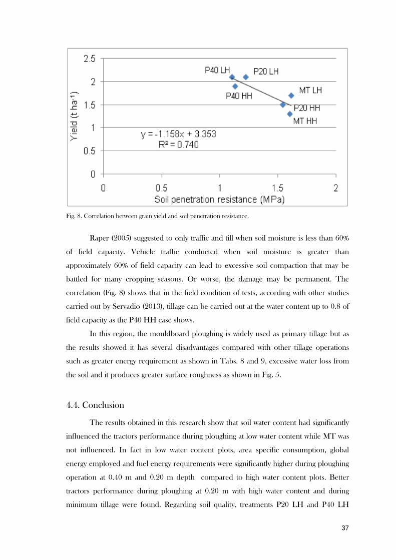
Fig. 7. Results of wheat harvesting (Error bars represent the standard deviation. Average of 18 values.) Besides, According with other authors (Marsili et al., 1998), a significant linear

correlation between soil penetration resistance and yield for different treatments was

found (Fig. 8).

37

Fig. 8. Correlation between grain yield and soil penetration resistance.

Raper (2005) suggested to only traffic and till when soil moisture is less than 60%

of field capacity. Vehicle traffic conducted when soil moisture is greater than

approximately 60% of field capacity can lead to excessive soil compaction that may be

battled for many cropping seasons. Or worse, the damage may be permanent. The

correlation (Fig. 8) shows that in the field condition of tests, according with other studies

carried out by Servadio (2013), tillage can be carried out at the water content up to 0.8 of

field capacity as the P40 HH case shows.

In this region, the mouldboard ploughing is widely used as primary tillage but as

the results showed it has several disadvantages compared with other tillage operations

such as greater energy requirement as shown in Tabs. 8 and 9, excessive water loss from

the soil and it produces greater surface roughness as shown in Fig. 5.

4.4. Conclusion The results obtained in this research show that soil water content had significantly

influenced the tractors performance during ploughing at low water content while MT was

not influenced. In fact in low water content plots, area specific consumption, global

energy employed and fuel energy requirements were significantly higher during ploughing

operation at 0.40 m and 0.20 m depth compared to high water content plots. Better

tractors performance during ploughing at 0.20 m with high water content and during

minimum tillage were found. Regarding soil quality, treatments P20 LH and P40 LH

38

showed good effects on structural stability and on grain yield, furthermore soil structure

created by treatment P20 LH allowed an optimal water infiltration rate, meaning that

runoff is reduced and an high percentage of rainwater is stored. A significant correlation

between grain yield and soil penetration resistance was found highlighting how soil

physical-mechanical parameters may be good indicators of its productivity. Even if do not

exists the best tillage operation ever, it exists a compromise among targets: machineries,

meteorological conditions, yield, soil status, costs, etc., and obtained results during these

field tests allow to consider MT and P20 treatments suitable for this type of soil in climate

change scenarios because MT is not influenced by soil water content and P20 was a good

compromise among targets.

39

5. Delineation of Site-Specific Management Zones in Wheat Field based on

Soil Structural Stability, Shear Strength, Water Content, and Nitrogen

5.1. Introduction Natural variability of soil properties can be affected by several factors, such as land

use, water content level, management system adopted, and climatic conditions. Intensive

agricultural production systems, generally, rely on heavy machinery. Repeated passes of

high working capacity machines on the field can cause soil compaction and, consequently,

low permeability to water and nutrients and high resistance to root penetration (Servadio

2010). Traffic of agricultural machines may vary in terms of intensity and geographical

distribution on the field. As a consequence, high variability of soil physical properties and

crop yield can occur, even in soils characterized by homogeneous distribution of physical

properties (Mouazen et al. 2001; Carrara et al. 2007). In this scenario, uniform field

management often results in over-application of inputs in areas with high nutrient levels,

and under-application of inputs in areas with low nutrient levels (Ferguson et al. 2003;

Servadio et al. 2010). Sub-zones within the field can be identified by gathering

information with high precision measuring techniques (Bullock et al. 2007). Within-field

variability may determine a site-specific management, generally acknowledged as a

possible way to address this problem (Cahn et al. 1994; McKinion et al. 2001; Godwin

and Miller 2003; Mzuku et al. 2005; Keller et al. 2012).

The management zone (MZs) approach (Mulla et al. 1992) is a site-specific

management method, based on the determination of sub-regions characterized by

homogeneous combination of yield-limiting factors (Vrindts et al. 2005). The definition of

the management zones generally rely on spatial information relative to soil properties

(organic matter, total Nitrogen, texture, soil strength, etc.) that are stable or predictable

over time, and related to crop yield (Franzen et al. 2003; Schepers et al. 2000, 2004).

Among several techniques, cluster analysis of soil and crop data has been used by

Taylor et al. (2003) as a basis for such zones definition, and by Fleming et al. (2004) to

delineate areas of different yield potential. Fuzzy k-means clustering algorithm has been

widely used to classify management areas by Anderberg (1973) and Stafford et al. (1999).

Furthermore, in order to detect clusters of different geometrical shapes, Gustafson and

Kessel (1979) extended the fuzzy k-means algorithm (Höppner et al. 1999, Vrindts et al,

2005).

40

The application of such analysis allows to take into account the continuous

variation of natural soil variables (Burrough 1989) and it has been used to identify

potential within-field management zones in precision agriculture (Boydell and McBratney

2002). Several parameters representing the soil conditions can be considered in the

definition of management zones. Parameters related to the crop yield are usually selected,

in particular the chemical and physical soil properties (Trangmar et al. 1987: Cambardella

et al. 1994: Ortega et al. 1999; Còrdoba et al. 2013). For example, in (Li et al. 2007a),

organic matter, bulk electrical conductivity, total Nitrogen, available Nitrogen, and

available Phosphorus were selected as main limiting factors for the crop yield. Electrical

conductivity, associated with other soil parameters (such as pH, total Nitrogen, organic

matter), was also considered by several authors (Ortega and Santibànez 2007; Morari et

al. 2009; Moral et al. 2010; Van Meirvenne et al. 2013). Davatgar et al. (2012),

considered as limiting factor the cation exchange capacity, while in (Li et al. 2007b),

NDVI image was taken into account.

Soil mechanical properties were less considered as input parameters for the

delineation of management zone, even if many efforts have been made also to analyze

their spatial variability. For example, Vrindts et al., 2005, Yao et al. 2014 considered Bulk

density; Duffera et al., considered Penetration resistance and Bulk density.

In the present paper, the within field spatial variability of some soil properties was

investigated by means of soil sampling, measurements and geostatistical analysis. The

novelty of this work lies in the selection of shear strength and structural stability as limiting

yield factors. In particular, shear strength results highly correlated with soil strength and

soil tillage (Servadio et al. 2005; Servadio 2013). Havaee et al. (2015) reported that soil

shear strength plays a key role in soil structure and/or erodibility, and is usually used as

primary indicator of soil resistance to erosion. Structural stability was selected because is a

key factor in determining soil quality, in fact the loss of structure is a type of physical soil

degradation which is usually related to specific land uses, particularly to soil tillage.

Several authors have observed a loss of soil structural stability under the influence of

cultivation which frequently involves a decrease in SOM contents (Barral et al., 2007). In

addition to the previous parameters, water content and total Nitrogen were also

considered.

The objectives of this study were to analyze within field spatial variability of crop

yield acquiring yield data of three consecutive growing seasons of wheat (Triticum durum)

and to define potential management zones for adoption of precision farming techniques.

41

Potential management zones (MZs) were defined using soil parameters as data source

through fuzzy clustering technique. Two cluster analyses are carried out, taking into

account the soil properties. In particular, shear strength, structural stability and water

content were considered in the first cluster, while in the second one total Nitrogen was

added to the previous parameters. Finally, the performance of the multivariate

classification method has been evaluated considering the crop yield in the defined zones.

5.2. Materials and methods 5.2.1. Site and data acquisition The site of the performed tests was a field characterized by clay loam soil (2.7 ha),

classified as Vertic Cambisol (FAO 1998), belonging to a farm in center of Italy,

4152’502” Latitude (N); 1212’866” Longitude (E). The climatic conditions are those of a

typical Mediterranean environment, characterized by a dry season between May and

September and a cold season from October-November to March-April. Every year the

soil was ploughed at 0.40 m depth and harrowed at 0.20 m depth with a rotary harrow.

Finally, the seedbed was prepared and then sowed with wheat. Fertilizations were

carried out just after sowing, 150 kg/ha of ammonium nitrate and at half of the crop cycle

200 kg/ha of urea. The crop was sowed in the second half of October and harvested in

mid July for each growing season. At the end of the crop cycle, during the wheat

harvesting, a grain yield map was acquired with a combine harvester (New Holland, NH

CX860) equipped with a grain header with a floor travel of 575 mm and a cutting width of

7.62 m. The GPS sensor (for the acquisition of EGNOS signal) has 15.24 – 20.32 (6”-8”)

accuracy and a grain mass flow sensor composed by a plate mounted to a pivoting device

with a counter weight, thus neutralising the rubbing effect of the grain. In addition, the

throwing angle of the paddles that throw the grain onto this sensor plate is set so that

shear grain volume does not cause deviation in the sensing system.

Acquired data were processed with the Precision Land Management Software

(Case New Holland, inc.). Yield map data were available for the years 2008, 2009 and

2010. The speed of the combine harvester machine during harvesting was 4.6, 5.0 and

4.2 km/h in 2008, 2009 and 2010, respectively. During the overall experimentation, from

October 2007 to July 2010, meteorological data (monthly rainfall, minimum and

maximum temperatures) were also recorded.

42

5.2.2. Meteorological data The acquired monthly mean temperatures and rainfall for each wheat cropping

season are depicted in Fig. 9.

Figure. 9. Monthly min and max temperature and monthly precipitation sum in each growing season (2007-08, 2008-09, 2009-10);

Considering the temperature trend, no differences were found concerning the

minimum and maximum values among the three cropping seasons, with recorded values

within -3 °C and 34 °C. Referring to the rain precipitation, in the period October - July,

mean values of rainfall were higher in 2009-2010 (824 mm) and 2008-2009 (642 mm)

than 2007-2008 (446 mm). More specifically, during March, April and May 2009, rainfall

values resulted very low (27, 51, 15 mm, respectively) with respect to the same period of

2008 (91, 34, 75 mm, respectively) and 2010 (68, 67, 73 mm, respectively). Furthermore,

in June 2009, a very high rainfall value (52 mm) was recorded with respect to the same

month of 2008 (28 mm) and 2010 (8 mm). The acquired rainfall data shown an erratic

weather pattern, in particular during the grain filling stage. As a rainfed crop, durum

wheat is particularly sensitive to year-to-year climatic changes. Generally, in the

43

Mediterranean environment, yield variation is mainly caused by low and irregular rainfall

distribution and high temperatures during such phenological phase (Diacono et al. 2012).

5.2.3. Sampling test, measurements, and mapping At the end of the third growing season, a georeferenced grid sampling on the soil,

previously tilled, was performed to investigate soil physical-chemical properties. The grid

sampling was based on a grid composed by squares sizing 30 x 30 m (900 m2). We

collected one sample for each corner of the squares, so each sample was 30 m away from

the other. We took approximately ten samples per hectare that according to Diacono et

al. (2012), were deemed acceptable. Geographical coordinates of each sampling point

were recorded using a GPS device (Trimble GEO XM) and then differential correction

was performed using the post processing software Trimble Pathfinder Office

(www.trimble.com). Twenty samples of soil (from 0 m to 0.2 m depth) were taken using

an Edelman auger (Eijkelkamp) type chosen in respect of the soil type in question. Using

a wing auger of 0.1 m length and 0.2 diameter, samples were taken to determine

structural stability, water content, and total Nitrogen (N).

Furthermore, as indicator of soil strength, twenty georeferenced measurements of

shear strength were performed, from 0 m to 0.2 m depth. Structural stability of soil

aggregates was determined on the 0.25mm fraction by means of the Kemper method

(Kemper and Chepil 1965). The structural stability was determined on the principle that

unstable aggregates will break down more easily than stable aggregates when immersed

into water. To determine the stability, 8 sieves were filled with a certain amount of soil

aggregates. These sieves were placed in a can filled with water, which moved up and

downward for a fixed time. Unstable aggregates fallen apart and passed through the sieve

and were collected in the water-filled can underneath the sieve. After drying the cans with

the aggregates, the weight of both stable and unstable aggregates was determined. Dividing

the weight of stable aggregates over total aggregate weight gives an index for the aggregate

stability

Soil water content was determined considering samples of soil extracted with a

corer sampling ring. Hence, the samples were weighed and dried until they reached a

constant weight. Soil total Nitrogen was measured with the Kjeldahl method (Bremner, et

al 1996). Finally, soil shear strength was measured using a field inspection vane tester

from 0 to 260 kPa (Eijkelkamp).

44

Interpolation of soil properties and grain yield maps was performed using inverse

distance weighting interpolation, yielding 1026 data points (Vrindts et al. 2005). The

minimum and the maximum number of neighbours and the optimal power value were

determined by minimizing the root-mean square prediction error (RMSPE) estimated by

cross-validation. The geostatistical analyses were conducted using the Geostatistical

Analyst extensions of the ArcGIS 10.0 software (Esri Inc., Redlands, CA, USA).

5.2.4. Management zone identification According to Vrindts et al. (2005), Gustafson-Kessel algorithm was applied using

soil variables as inputs. Four soil attributes, considered yield limiting factors (water

content, shear strength, structural stability, and total Nitrogen), were selected as data

sources. Two cluster analyses were carried out to the interpolated maps in order to

identify potential management zones. The first cluster analysis was performed considering

the following indicator parameters: water content, shear strength and structural stability.

In order to evaluate the impact of the chemical fertilization on the crop yield and

to compare such impact with the soil mechanical properties effects on the crop yield, a

second cluster analysis was performed by adding to the previous soil parameters the total

Nitrogen.

Soil water content was used as input parameter in the cluster analysis because

influences soil hydraulic properties, which produce crucial effects on infiltration, surface

runoff and soil erosion process that are critical in variuos fields of practical interest, even

though this parameter varies in time and was surveyed once. In fact Vachaud et al. (1985)

were among the first to show that spatial patterns of soil moisture changed little with time

despite large variation over time and space in the field. This phenomenon has been called

temporal stability. The temporal stability for soil moisture, however, is widely recognised

by most authors (Gao and Shao, 2012; Brocca et al., 2009; Coppola et al., 2011; Cosh et

al., 2004, 2008; da Sivaro et al., 2001; Martínez-Fernández and Ceballos, 2003). In other

words, the pattern of variation across the study area remains more or less the same, even

though the average soil water content changes. Soil water content temporal stability has

been demonstrated and only a small number of soil moisture samples at are needed to

monitor the average soil water content across relatively large areas (Guber et al., 2008;

Starr, 2005).

45

Yield data were used to evaluate the performance of multivariate classification

based on soil variables, rather than as layer for delineating management zones, according

to Cordoba et al. (2013). Fuzzy classification produces a continuous grouping of objects

by assigning partial class membership values, according to the properties variability in the

soil continuum. In the present investigation, Gustafson-Kessel algorithm was applied by

using the FuzMe software functions from the Australian Centre for Precision Agriculture

(Minasny and McBratney, 2002) in MatLab environment (www.mathworks.com). Cluster

analysis was performed following the data-processing steps presented by Vrindts et al.

2005. The first steps in cluster analysis require the definition of the number of classes and

the fuzziness exponent. According to Davatgar et al. (2012), Fridgen et al. (2004),

Reyniers et al. (2006), Vrindts et al. 2005, the number of class range from 2 to 8 or 9.

Considering the fuzziness exponent �, different values can be considered. For example,

Odeh et al., 1992 set it equal to 1.35, while Bezdek et al., 1984 suggest a possible range

equal to [1.5, 3]. Most researchers have proposed � =2 (Yu et al, 2004). In this

investigation, calculations were performed considering the number of clusters from 2 to

10 and the fuzziness exponent ranging from 1.1 to 3 in 0.1 steps. The optimal number of

clusters were selected by minimizing the FPI and NCE indexes (Fridgen et al., 2004,

Wang and Zhang, 2007), while the optimal fuzziness exponents were determined using

the derivative of the objective function J values with respect to the fuzziness exponent �

(McBratney and Moore, 1985). According to Vrindts et al, 2005, the calculations with the

optimal fuzziness index and with the optimal cluster number was repeated 10 times with

different initial cluster centres, choosing the results with best separation considering the

validity function S (Xie and Beni, 1991).

5.3. Results and discussion 5.3.1. Wheat yield In the present investigation, yield data acquired during the three consecutive

growing seasons (2007-10) showed a great temporal variability, as depicted in Fig. 10, and

also high spatial variability between three years, in fact different yields were acquired from

same areas of the field..

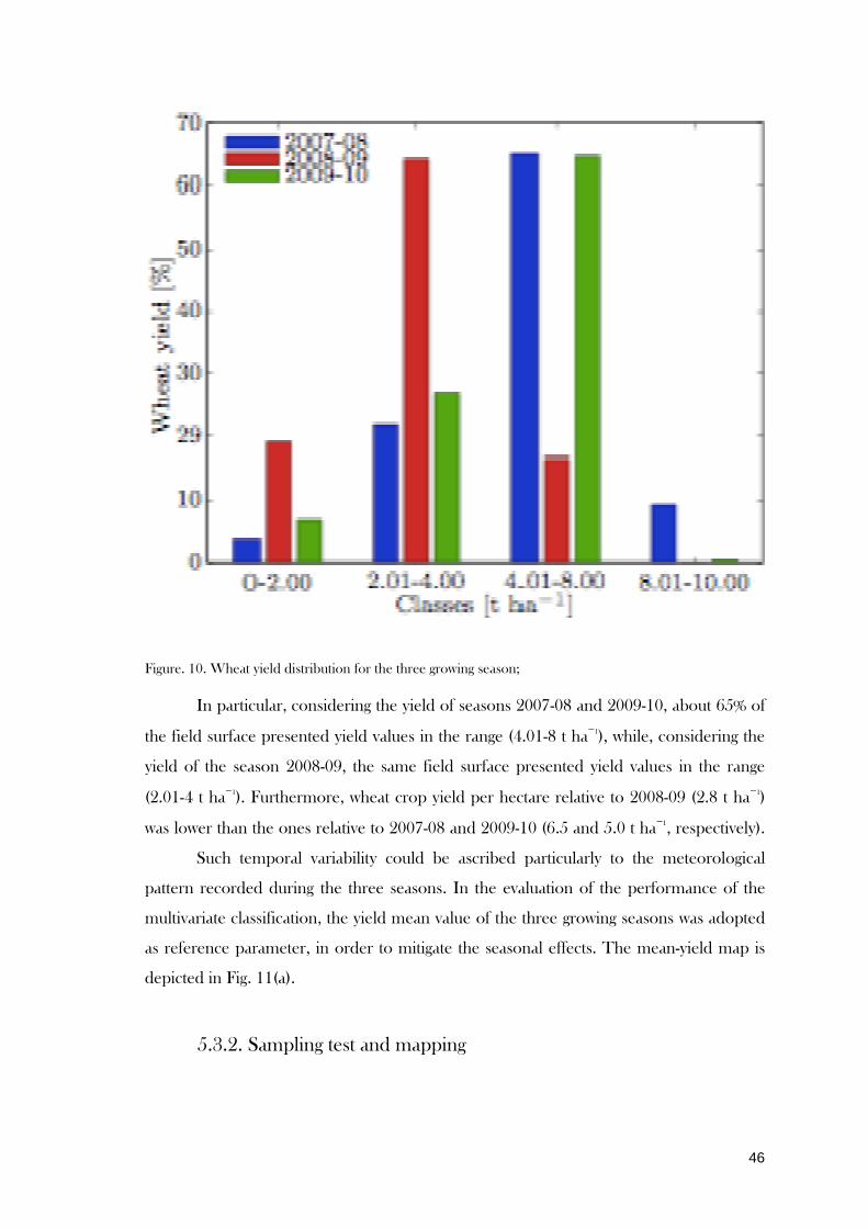
46

Figure. 10. Wheat yield distribution for the three growing season; In particular, considering the yield of seasons 2007-08 and 2009-10, about 65% of

the field surface presented yield values in the range (4.01-8 t ha−1), while, considering the

yield of the season 2008-09, the same field surface presented yield values in the range

(2.01-4 t ha−1). Furthermore, wheat crop yield per hectare relative to 2008-09 (2.8 t ha−1)

was lower than the ones relative to 2007-08 and 2009-10 (6.5 and 5.0 t ha−1, respectively).

Such temporal variability could be ascribed particularly to the meteorological

pattern recorded during the three seasons. In the evaluation of the performance of the

multivariate classification, the yield mean value of the three growing seasons was adopted

as reference parameter, in order to mitigate the seasonal effects. The mean-yield map is

depicted in Fig. 11(a).

5.3.2. Sampling test and mapping

47

Within field spatial variability of soil physical-chemical parameters is represented

by means of the interpolated maps. The maps of water content (b), total Nitrogen (c),

structural stability (d), and shear strength (e) are shown in Fig. 11.

Figure 11. Interpolated maps of soil physical-chemical parameters and Wheat yield elaborated using IDW interpolation

48

Descriptive statistics for soil physical-chemical properties are given in Table 10.

Water content and total Nitrogen had medium coefficient of variability (CV) (5.3 and

9.2%, respectively), while shear strength and structural stability presented high value of

CV (66 and 28.5%, respectively).

Table 10. Descriptive statistics of the soil parameters

Soil parameter Mean SD CV [%]

Water content [%] 22 1.16 5.3

Shear strength [kPa] 33 22 66

Structural Stability [%] 33.2 9.5 28.5

Total Nitrogen [%] 0.12 0.01 9.2

5.3.3. Management zone identification In this scenario, the definition of management zones could be of use in the

identification of specific input applications, such as soil tillage and fertilization, and,

consequently, in the improvement of energy efficiency, environment protection, and

wheat quality. In order to define such zones, two cluster analyses were performed.

5.3.4. Cluster analysis In the first cluster analysis, shear strength was selected as soil strength indicator,

and structural stability was selected as soil quality indicator. Furthermore, water content

was chosen as additional limiting yield factor. By applying the data-processing steps

described in Section 5.2.4, the optimal clustering results were obtained with a number of

clusters equal to 3 and with a fuzziness exponent equal to 2.2.

Fig. 12 shows the values of FPI and NCE with respect to the number of classes c.

The mean values and the coefficients of variability of the parameters relative to the first

cluster analysis are reported in Table 11, together with the yield data.

49

Figure 12. FPI and MPE indices for the first cluster analysis Table 11. First cluster analysis: mean values and coefficients of variation of soil parameters for each zone

Zone

Water content Shear strength Structural Stability Yield

Mean

[%]

CV

[%]

Mean

[kPa]

CV

[%]

Mean

[%]

CV

[%]

Mean

[t ha-1]

CV

[%]

1 21.2 1.6 41.7 41.6 25.4 7.9 4.5 14.7

2 22.3 1.7 16.8 32.1 37.1 11.1 5.1 12.7

3 22.5 1.3 34.3 39.9 42.8 8.8 4.9 12.9

The management zones map is depicted in Fig. 13. Referring to the yield limiting factors,

it can be noticed that:

• zone 1 presented the lowest mean values of water content and structural stability,

and the highest mean value of shear strength;

• zone 2, registered a mid-range value of water content, an upper-mid-range value of

structural stability, and the lowest value of shear strength;

• zone 3 grouped an area with the highest value of water content and structural

stability, and a mid-range value of shear strength.

Referring to the crop yield:

• zone 1 presented the lowest mean value;

50

• zone 2 registered the highest value;

• zone 3 presented an upper-mid-range value.

Figure 13. First cluster analysis: the management zones

The management zones were analysed mapping the limiting yield factors with

respect to the crop yield. Figures 14, 15, and 16 show the soil structural stability, the shear

strength, and the water content versus the grain yield, respectively.

Figure 14. Cluster 1: structural stability and crop yield

51

Figure 15. Cluster 1: shear strength and crop yield

Figure 16. Cluster 1: water content and crop yield

By analysing the results reported in Table 11, it can be noticed that water content

values range from 21.2 to 22.5 %, presenting low coefficients of variation. Considering the

other soil parameters, high values of shear strength and low values of structural stability

correspond to low values of crop yield, see zone 1. On the other hand, high or upper-

mid-range values of structural stability coupled with mid-range or low values of shear

strength correspond to upper-mid-range or high values of crop yield, see zones 3 and 2.

The second cluster analysis was performed considering shear strength as soil

strength indicator, structural stability as soil quality indicator, and water content as

additional limiting yield factor. In order to compare the impact of the chemical

fertilization with the soil mechanical properties effects on the crop yield, Total Nitrogen

52

was added to the previous parameters as environmental indicator. As in the previous case,

the optimal clustering results were obtained with a number of clusters equal to 3 and with

a fuzziness exponent equal to 2.2.

Fig. 17 shows the values of FPI and NCE with respect to the number of classes c.

The management zones map is shown in Fig. 18. The mean values for each parameter

for four clusters are reported in Table 12, together with the yield data.

Referring to the limiting yield factors mean values, it can be noticed that:

• zone 1 presented the lowest mean values of water content, structural stability and

Nitrogen, and the highest mean value of shear strength;

• zone 2, registered the highest mean value of water content, structural stability and

Nitrogen, and upper-mid-range value of shear strength;

• zone 3 grouped an area with an upper-mid-range value of water content and

structural stability, the lowest mean value of shear strength and a mid-range value

of Nitrogen.

Referring to the crop yield:

• zone 1 presented the lowest mean value;

• zone 2 registered the highest mean value;

• zone 3 presented an mid-range value.

Figure 17. FPI and MPE indices for the second cluster analysis

53

Figure 18. Second cluster analysis: the management zones Table 12. Second cluster analysis: mean values and coefficients of variation of soil parameters for each zone

Zone

Water content Shear strength Structural Stability Total Nitrogen Yield

Mean

[%]

CV

[%]

Mean

[kPa]

CV

[%]

Mean

[%]

CV

[%]

Mean

[%]

CV

[%]

Mean

[t ha-1]

CV

[%]

1 21.2 1.5 42.8 39.7 25.2 7.6 0.117 4.2 4.6 15.1

2 22.5 1.3 33.3 43.7 42.7 10.1 0.120 5.8 5.1 13.0

3 22.2 1.8 18.3 39.7 36.0 12.6 0.118 4.8 4.8 11.8

Considering the limiting yield factors with respect to the crop yield, Figures 18, 19,

20, and 21 show the soil structural stability, the shear strength, the water content, and the

total Nitrogen versus the grain yield, respectively.

54

Figure 18. Cluster 2: structural stability and crop yield

Figure 19. Cluster 2: shear strength and crop yield

Figure 20. Cluster 2: water content and crop yield

55

Figure 21. Cluster 2: total Nitrogen and crop yield

Considering the results reported in Table 12, the Nitrogen mean values in each

zone seem to follow the trend of the soil parameters with respect to the yield showed in

the previous cluster. In fact, high values of shear strength and low values of structural

stability and Nitrogen correspond to low values of crop yield, as in zone 1. On the other

hand, high or upper-mid-range values of structural stability and Nitrogen coupled with

mid-range or low values of shear strength correspond to high or upper-mid-range values

of crop yield, as in zones 2 and 3.

5.4. Conclusion

In the present investigation, a geo-referenced grid sampling on the soil was

performed to investigate soil physical-mechanical parameters and chemical properties.

Three year yield data were acquired with a combine harvester equipped with GPS

sensor. Interpolation of soil properties was executed to generate field maps. Two cluster

analyses were performed. In the first one, shear strength was selected as soil strength

indicator, structural stability was selected as soil quality indicator, and water content was

chosen as additional limiting yield factor. In the second one, total Nitrogen was added to

the previous limiting factors as environmental indicator to compare the impact of the

chemical fertilization on the crop yield with the soil mechanical properties effects. Results

of both clusters revealed that the optimum number of management zones was three. The

56

mean value of the three years yield was considered in the evaluation of the performance

of the multivariate classification in order to mitigate the seasonal effects. In the first cluster

analysis, results show that, among the input parameters, shear strength and structural

stability were the most significant limiting factors for the wheat yield. Such results were

confirmed in the second cluster analysis, where Total Nitrogen was considered as

additional environmental parameter.

As indicators of soil strength and quality, shear strength and soil structural stability

are correlated with agricultural practices, in particular in soil tillage. Hence, the defined

management zones could provide information for site-specific management, including the

application of different soil tillage methods. Furthermore, variable-rate application (VRA)

instead of uniform-rate application (URA) of inputs might be carried out, decreasing

fertilization in the more productive area and minimizing the application of chemical

substances as a strategy to obtain a more cost-effective field management.

Finally, for the specific examined site, the adoption of precision farming

techniques could lead to an optimization of the soil-machinery interaction and to a

reduction of soil compaction and greenhouse gas emissions.

57

6. Perspectives Further researches were conducted in order to optimize the procedure of

management zone definition and the selection criterion of soil parameters for cluster

analysis.

Soil condition and crop yield were examined in three fields, characterized by

different soil texture, belonging to a farm in the center of Italy. Spatial variability of

chemical and physical properties was investigated by means of soil sampling and

geostatistical analysis. Potential management zones (MZs) were defined by means of an

optimised fuzzy clustering algorithm, evaluating three soil attributes: clay percentage and

organic matter, considered as indicator parameters, and water content, considered as

yield limiting factors. For each field, the effects of such attributes on the soil mechanical

properties were evaluated, considering the set of parameters constituted by soil structural

stability, shear strength, and penetration resistance as test data set. Sand percentage and

yield were also included in the test data set. An extra-field analysis was also performed to

compare the intra-field results and to identify the most important factors affecting the soil

mechanical properties and the crop yield.

Furthermore a study was conducted for comparing the results obtained by

management zone definition performed selecting empirically input soil parameters with

the results obtained by management zone definition performed selecting input soil

parameters using a Principal Component Analysis in MatLab environment.

Final results of both researches are still in elaboration.

58

7. Main conclusions

The results of tests performed during the whole experimentation highlighted the

presence of high spatial variability of soil physical-chemical properties within the

agricultural fields examined. Assessing such spatial variability becomes essential for

enhancing the efficiency of crop management, lowering economic and environmental

costs. Such result can be achieved only through site specific management which requires

the delineation of management zones. Georeferenced soil sampling resulted as a proper

technique for investigating spatial variability within agricultural fields, even though the soil

parameters vary in time and were surveyed once. In fact some authors (Brocca et al.,

2009; Coppola et al., 2011; Cosh et al., 2008; Martínez-Fernández and Ceballos, 2003;

Vachaud et al., 1985) stated that spatial patterns of soil properties changed little with time

despite large variation over time and space in the field. This phenomenon has been called

temporal stability. In other words, the pattern of variation across the study area remains

more or less the same, even though the average content changes.

Georeferenced sampling of soil physical-chemical parameters allowed to identify

soil quality and soil strength indicators, furthermore monitoring the performance of

machineries during soil tillage and agricultural operations allowed to identify field

efficiency indicators (i.e.: area specific consumption, global energy employed and fuel

energy requirements).

Obtained results showed that soil water content had significantly influenced the

tractors performance during tillage and traffic in the field. Furthermore correlations

between soil properties (OM and N) and yield confirmed that in agricultural ecosystems,

N and OM are the major determinants and indicators of soil fertility and quality, which

are closely related to soil productivity. Moreover a significant correlation between grain

yield and soil penetration resistance was found and results of cluster analysis showed that,

among the input parameters, shear strength and structural stability were the most

significant limiting factors for the wheat yield highlighting how soil physical-mechanical

parameters may be good indicators of its productivity.

Such indicators can be utilized as input parameters in cluster analysis or can be

utilized to select the more efficient soil tillage operation, such as direct seeding.

Geostatistical analysis conducted using the FuzMe, MatLab and ArcGIS 10.0

softwares for interpolating the acquired data was an useful tool to assess spatial variability

within agricultural fields and for delineating and representing management zones.

59

In future researches Principal Component Analysis (PCA) could be of use to

overcome the problem in selection empirically inputs variables of cluster analysis

enhancing the delineation process of management zone as well as the acquisition of

remote sensing data that can provide more accurate and numerous data and develop new

vegetational indexes.

In conclusion, the assessing process of spatial variability within agricultural fields,

the identification of soil indicators and the definition of management zones can be

considered as an adaptation technique to Climate Change enhancing the efficiency of

agriculture. In fact, the defined management zones could provide information for site-

specific management, including the application of different soil tillage methods.

Furthermore, variable-rate application (VRA) instead of uniform-rate application (URA)

of inputs might be carried out, decreasing fertilization in the more productive area and

minimizing the application of chemical substances as a strategy to obtain a more cost-

effective field management.

60

8. References Adler P.R., Del Grosso S.J. and Parton W.J. (2007), Life-cycle assessment of net

greenhouse-gas flux for bioenergy cropping systems, Ecol. Appl., 17(3), 675–691.

Agbu, P.A., Olson, K.R., 1990. Spatial variability of soil properties in selected Illinois

Mollisols. Soil Sci. 155, 777–786.

Alletto, L., Coquet, Y. & Roger-Estrade, J. 2010. Two-dimensional spatial variation of soil

physical properties in two tillage systems. Soil Use and Management, 26, 432-444.

Allmaras R.R. and Dowdy R.H. (1985), Conservation tillage systems and their adoption

in the United States, Soil Till. Res. 5(2), 197–222.

Anderberg, M.R., (1973). Cluster analysis for applications. Monographs and textbooks on

probability and mathematical statistics.

Barral, M. T., Buján, E., Devesa, R., Iglesias, M. L., & Velasco-Molina, M. (2007).

Comparison of the structural stability of pasture and cultivated soils.Science of the

total environment, 378(1), 174-178.

Bezdek, J.C., Ehrlich, R., Full, W., (1984). FCM: The fuzzy c-means clustering algorithm.

Comput. Geosci. (10), 191-203.

Bagarello V., Iovino M. and Elrick D.E. (2004), A simplified falling-head technique for

rapid determination of field-saturated hydraulic conductivity. Soil Sci. Soc. Am. J.,

68, 66 - 73.

Barbour M.G., Burk J.H., Pitts W.D., Gilliam F.S. and Schwartz M.W. (1998),

Terrestrial Plant Ecology. Benjamin Cummings, pp. 182-204.

Basso, B., Cammarano, D., Chen, D., Cafiero, G., Amato, M., Bitella, G., Rossi, R.

Basso, F. 2009. Landscape position and precipitation effects on spatial variability of wheat

yield and grain protein in southern Italy. Journal of Agronomy and Crop Science,

195, 301-312.

Basso, B., Ritchie, J. T., Cammarano, D. & Sartori, L. 2011. A strategic and tactical

management approach to select optimal N fertilizer rates for wheat in a spatially

variable field. European Journal of Agronomy, 35, 215-222.

Beckett, P.H.T., Webster, R., 1971. Soil variability: a review. Soils Fertil. 34, 1–15.

Becher H.H. (1998), Resistances to penetration of aggregates from loess-drived topsoils at

different soil water tensions. Soil and Tillage Research, 47, 73–81.

61

Beni C., Servadio P., Marconi S. and Neri U. (2012), Anaerobic Digestate

Administration: Effect on Soil Phisical and Mechanical Behaviour in Southern

Italy, Communications in Soil Science and plant analysis, 43(5): 821–834.

Boehm, M.M., Anderson, D.W., 1997. A landscape-scale study of soil quality in three

prairie farming systems. Soil Sci. Soc. Am. J. 61, 1147–1159.

Bouwer H. (1986), Intake rate: cylinder. In: Klute, A. (Ed.), Methods of Soil Analysis,

Part 1. Physical and Mineralogical Properties, monograph, 9. ASA, Madison, WI,

pp 825-843.

Boydell, B., McBratney, A., (2002). Identifying potential within-field management zones

from cotton-yield estimates. Precision agriculture (3), 9–23.

Bremner, J. M., Sparks, D. L., Page, A. L., Helmke, P. A., Loeppert, R. H., Soltanpour,

P. N., ... & Sumner, M. E. (1996). Nitrogen-total. Methods of soil analysis. Part

3-chemical methods., 1085-1121.

Brocca, L., Melone, F., Moramarco, T., Morbidelli, R., 2009. Soil moisture temporal

stability over experimental areas in Central Italy. Geoderma 148, 364–374.

Bullock, D.S., Kitchen, N., Bullock, D.G., (2007). Multidisciplinary teams: A necessity

for research in precision agriculture systems. Crop science (47), 1765–1769.

Burgun C., Lacour S., Delacroix A., Descombes G. and Doyen V. (2013), Computing

time and fuel requirements to assess efficiency of a field work from conventional

laboratory tests : application to a plowing operation, Agricultural and Food

Science, 22(2), 247-261.

Burrough, P.A., 1983a. Multiscale sources of spatial variation in soil. I. The application of

fractal concepts to nested levels of soil variation. J. Soil Sci. 34, 577–597.

Burrough, P.A., 1983b. Multiscale sources of spatial variation in soil. II. A non-Brownian

fractal model and its application to soil survey. J. Soil Sci. 34, 599–620.

Burrough, P., (1989). Fuzzy mathematical methods for soil survey and land evaluation.

Journal of soil science (40), 477–492.

Burrough, P.A., 1993. Soil variability: a late 20th century view. Soils Fertil. 56, 529–562.

Cahn, M., Hummel, J., Brouer, B., (1994). Spatial analysis of soil fertility for site-specific

crop management. Soil Science Society of America Journal (58), 1240–1248.

Cambardella, C., Moorman, T., Parkin, T., Karlen, D., Novak, J., Turco, R., Konopka,

A., (1994). Field-scale variability of soil properties in central Iowa soils. Soil

Science Society of America Journal 589, 1501–1511

62

Carrara, M., Castrignanò, A.,Comparetti, A., Febo, P., Orlando, S. 2007. Mapping of

penetrometerresistance in relation to tractortrafficusing multivariate geostatistics.

Geoderma 142, 294–307.

Chatterjee A. and R. Lal (2009), On farm assessment of tillage impact on soil carbon and

associated soil quality parameters, Soil & Tillage Research, 104(2), 270–277.

Chen S., Xia G.M., Zhao W.M., Wu F.B. and Zhang G.P. (2007), Characterization of

leaf photosynthetic properties for no-tillage rice, Rice Sci., 14(4), 283–288.

Collins B.A. and Fowler D.B. (1996), Effect of soil characteristics, seeding depth,

operating speed, and opener design on draft forceduring direct seeding, Soil &

Tillage Research, 39(3), 199-211.

Conant R.T., Easter M., Paustian K., Swan A. and Williams S. (2007), Impact of periodic

tillage on soil C stocks: a synthesis, Soil Tillage Res., 95(1-2), 1–10.

Coppola, A., Comegna, A., Dragonetti, G., Lamaddalena, N., Kader, A.M., Comegna,

V., 2011. Average moisture saturation effects on temporal stability of soil water

spatial distribution at field scale. Soil and Tillage Research 114, 155–164.

Cordoba, M., Bruno, C., Costa, J., Balzarini, M., (2013). Subfield management class

delineation using cluster analysis from spatial principal components of soil

variables. Computers and Electronics in Agriculture (97), 6–14.

Cosh, M.H., Jackson, T.J., Moran, S., Bindlish, R., 2008. Temporal persistence and

stability of surface soil moisture in a semi-arid watershed. Remote Sensing of

Environment 112, 304–313.

Davatgar, N., Neishabouri, M.R., Sepaskhah, A.R., (2012). Delineation of site specific

nutrient management zones for a paddy cultivated area based on soil fertility using

fuzzy clustering. Geoderma 173-174, 111-118.

De Benedetto, D., Castrignanò, A., Rinaldi, M., Ruggieri, S., Santoro, F., Figorito, B.,

Gualano, S., Diacono, M. & Tamborrino, R. 2013. An approach for delineating

homogeneous zones by using multi-sensor data. Geoderma, 199, 117-127.

Di Fonzo, N., De Vita, P., Gallo, A., Fares, C., Padalino, O. & Troccoli, A. 2001. Crop

management efficiency as a tool to improve durum wheat quality in

Mediterranean areas. COLLOQUES-INRA, 67-82.

Diacono, M., Castrignanò, A., Troccoli, A., De Benedetto, D., Basso, B. & Rubino, P.

2012. Spatial and temporal variability of wheat grain yield and quality in a

Mediterranean environment: A multivariate geostatistical approach. Field Crops

Research, 131, 49-62.

63

Dobermann, A., Goovaerts, P., Neue, H.U., 1997. Scale-dependent correlations among

soil properties in two tropical lowland rice fields. Soil Sci. Soc. Am. J. 61,

1483– 1496.

Doolittle, J. A. & Brevik, E. C. 2014. The use of electromagnetic induction techniques in

soils studies. Geoderma, 223-225, 33-45.

Earl R. (1997), Prediction of trafficability and workability from soil moisture deficit. Soil

& Tillage Research 40, 155-168.

Edmonds, W.J., Baker, J.C., Simpson, T.W., 1985. Variance and scale influences on

classifying and interpreting soil map units. Soil Sci. Soc. Am. J. 49, 957–961.

Ferguson, R., Lark, R., Slater, G., (2003). Approaches to management zone definition for

use of nitrification inhibitors. Soil Science Society of America Journal (67),

937– 947.

Fleming, K., Heermann, D., Westfall, D., (2004). Evaluating soil color with farmer input

and apparent soil electrical conductivity for management zone delineation.

Agronomy Journal (96), 1581–1587.

Food and Agriculture Organization, 1998. “World Reference Base for Soil Resources,”

Report No. 84, Rome, Italy.

Fowler D.B. (1995), Seeding Equipment. Winter Wheat Production Manual, Ducks

Unlimited Canada, Yorkton, Sash., pp. 601-621.

Franzen, D., Nanna, T., Robert, P., et al., (2003). Management zone delineation

methods, in: Proceedings of the 6th International Conference on Precision

Agriculture and Other Precision Resources Management, Minneapolis, MN,

USA, 14-17 July, 2002., American Society of Agronomy. pp. 443–457.

Fridgen, J.J., Kitchen, N.R., Sudduth, K.A., Drummond, S.T., Wiebold, W.J., Fraisse,

C.W., (2004). Management zone analyst (mza). Agronomy Journal (96), 100–108.

Frogbrook, Z. L. & Oliver, M. A. 2007. Identifying management zones in agricultural

fields using spatially constrained classification of soil and ancillary data. Soil Use

and Management, 23, 40-51.

Gaston, L., Nkedi-Kizza, P., Sawka, G., Rao, P.S.C., 1990. Spatial variability of

morphological properties at a Florida flatwoods site. Soil Sci. Soc. Am. J. 54,

527– 533.

Godwin, R. J. & Miller, P. C. H. 2003. A review of the technologies for mapping

within-field variability. Biosystems Engineering, 84, 393-407.

64

Gomez K. A. and Gomez A.A. (1976), Statistical procedures for agricultural research

with emphasis on rice. Statistical procedures for agricultural research with

emphasis on rice.

Gooley, L., Huang, J., Pagé, D. & Triantafilis, J. 2014. Digital soil mapping of available

water content using proximal and remotely sensed data. Soil Use and

Management, 30, 139-151.

Guastaferro, F., Castrignanò, A., de Benedetto, D., Sollitto, D., Troccoli, A. & Cafarelli,

B. 2010. A comparison of different algorithms for the delineation of management

zones. Precision Agriculture, 11, 600-620.

Guo, Y., Shi, Z., Li, H. Y. & Triantafilis, J. 2013. Application of digital soil mapping

methods for identifying salinity management classes based on a study on coastal

central China. Soil Use and Management, 29, 445-456.

Gustafson, D., Kessel. W., (1979). Fuzzy clustering with a fuzzy covariance matrix. In:

Proceedings IEEE Conference on Decision and Control, San Diego, CA, USA,

pp. 761–766.

Hamza A.M. and Anderson W.K. (2005), Soil compaction in cropping systems. A review

of the nature, causes and possible solutions. Soil and Tillage Research, 82,

121-145.

Hajabbasi M.A. and Hemmat A. (2000), Tillage impacts on aggregate stability and crop

productivity in a clay-loam soil in central Iran. Soil and Tillage Research, 56,

205-212.

Havaee, S., Mosaddeghi, M. R., & Ayoubi, S. (2015). In situ surface shear strength as

affected by soil characteristics and land use in calcareous soils of central

Iran. Geoderma, 237, 137-148.

Heuvelink, G.B.M., Webster, R., 2001. Modelling soil variation: past, present, and

future. Geoderma 100, 269–301.

Hoppner, F., Klawonn, F., Kruse, R., Runkler, T., (1999). Fuzzy Cluster Analysis.

Methods for Classification, Data Analysis and Image Recognition. John Wiley and

Sons, Chichester, UK.

Hotelling, H., 1933. Analysis of a complex of statistical variables into principal

components. J. Educ. Psychol. 24, 417–441.

Jolliffe, I.T., 1986. Principal Component Analysis. Springer-Verlag, New York.

65

Keller, T., Sutter, J.A., Nissen, K., Rydberg, T., (2012). Using field measurement of

saturated soil hydraulic conductivity to detect low-yielding zones in three swedish

fields. Soil and Tillage Research (124), 68–77.

Keller, T., Sutter, J.A., Nissen, K., Rydberg, T. 2010. Soil structure explains some

within- field variation in crop yield. International Conference on Agricultural

Engineering (AgEng 2010). Towards Environmental Technologies.

Clermont-Ferrand, France, 6-8 September. Paper no. 374.

Kemper W.D. (1965), Aggregate stability. Methods of Soil Analysis. Part 1. Agronomy, 9:

511-519.

Koch H.J., Heuer H., Tomanova´ O. and Marlander B. (2008), Cumulative effect of

annually repeated passes of heavy agricultural machinery on soil structural

properties and sugar beet yield under two tillage systems. Soil and Tillage

Research, 101, 69-77.

Kroulik, M., Loch, T., Kviz, Z., Prosek, V. 2009. Procedures of soil farming to reduce

compaction. Proceedings of the Joint International Agricultural Conference

(JIAC). Wageningen Academic Publishers, The Netherlands.

Li, Y., Shi, Z., Li, F., (2007a). Delineation of site-specific management zones based on

temporal and spatial variability of soil electrical conductivity. Pedosphere 17(2),

156–164.

Li, Y., Shi, Z., Li, F., Li, H.Y., (2007b). Delineation of site-specific management zones

using fuzzy clustering analysis in a coastal saline land. Computers and Electronics

in Agriculture (56), 174–186.

Lyles L. and Woodruff, N.P. (1962), How moisture and tillage affect cloddiness for wind

erosion control. Agricultural Engineering, 42(3), 150-153.

López-Lozano, R., Casterad, M. A. & Herrero, J. 2010. Site-specific management units in

a commercial maize plot delineated using very high resolution remote sensing and

soil properties mapping. Computers and Electronics in Agriculture, 73, 219-229.

Marsili A., Servadio P., Pagliai M. and Vignozzi N. (1998), Compattamento del suolo

causato dal traffico di trattrici equipaggiate con cingoli di differente tipo ed effetti

sulla produzione vegetale. (Soil compaction due to the traffic of the tractors

equipped with different type of tracks and effects on the yield). Rivista di

Ingegneria Agraria n. 3, 144-149.

66

Manuwa, S. I. & Olaiya, O. C. 2012. Evaluation of Shear Strength and Cone Penetration

Resistance Behavior of Tropical Silt Loam Soil under Uni-Axial Compression.

Open Journal of Soil Science, 2, 95-99

Martínez-Fernández, J., Ceballos, A., 2003. Temporal stability of soil moisture in a large

field experiment in Spain. Soil Science Society of America Journal 67, 1647–

1656.

Mausbach, M.J., Wilding, L.P. (Eds.), Spatial Variabilities of Soils and Landforms. Soil

Science Society of America Special Publication No. 28. SSSA, Madison, WI, pp.

199–212.

McBratney, A.B., Moore, A.W., (1985). Application of fuzzy sets to climatic

classification. Agric. For. Meteorol., 35: 165-185.

McKinion, J., Jenkins, J., Akins, D., Turner, S., Willers, J., Jallas, E., Whisler, F., (2001).

Analysis of a precision agriculture approach to cotton production. Computers and

electronics in agriculture (32), 213–228.

Milne, A.E., Webster, R., Ginsburg, D., Kindred, D., 2012. Spatial multivariate

classification of an arable field into compact management zones based on past

crop yields. Comput. Electron. Agric. 80, 17–30.

Minasny, B., McBratney, A.B., (2002). FuzME version 3_0, Australian Centre for

Precision Agriculture. The University of Sydney, Australia

http://www.usyd.edu.au/su/agric/acpa

Moore, I.D., Gessler, P.E., Nielsen, G.A., Peterson, G.A., 1993. Soil attribute prediction

using terrain analysis. Soil Sci. Soc. Am. J. 57, 443–452.

Moral, F.J., Terròn, J.M., Marques da Silva, J.R., (2010). Delineation of management

zones using mobile measurements of soil apparent electrical conductivity and

multivariate geostatistical techniques. Soil and tillage research, (106) 335-343.

Morari, F., Castrignanò, A., Pagliarin, C., (2009). Application of multivariate geostatistics

in delineating management zones within a gravelly vineyard using geo-electrical

sensors. Computers and Electronics in Agriculture (68) 97–107.

Mouazen, A.M., Ramon, H., De Baerdemaeker, J. 2001. On-line detection of soil

compaction distribution based on finite element modelling procedure.

Proceedings of the 3rd European Conference on Precision Agriculture. 18–21

June, Montpellier, France, Agro Montpellier, Ecole Nationale Supérieure

Agronomique de Montpellier, pp. 455–460.

67

Mulla, D., Bhatti, A., Hammond, M., Benson, J., (1992). A comparison of winter wheat

yield and quality under uniform versus spatially variable fertilizer management.

Agriculture, ecosystems & environment (38), 301–311.

Munkholm L.J., Heck R.J. and Deen B. (2012), Long-term rotation and tillage effects on

soil structure and crop yield. Soil Tillage Research. doi:10.1016/j.still.

2012.02.007.

Mzuku, M., Khosla, R., Reich, R., Inman, D., Smith, F. & MacDonald, L. 2005. Spatial

variability of measured soil properties across site-specific management zones. Soil

Science Society of America Journal, 69, 1572-1579.

Naderi-Boldaji, M., Sharifi, A., Alimardani, R., Hemmat, A., Keyhani, A., Loonstra, E.

H., Weisskopf, P., Stettler, M. & Keller, T. 2013. Use of a triple-sensor fusion

system for on-the-go measurement of soil compaction. Soil and Tillage Research,

128, 44-53.

Odeh, I.O., Chittleborough, D.J., McBratney, A.B., (1992). Fuzzy-c-means and kriging

for mapping soil as a continuous system. Soil Science Society of America Journal

(56), 1848–1854.

Ortega, R., Westfall, D., Gangloff, W., Peterson, G., Stafford, J., et al., (1999).

Multivariate approach to n and p recommendations in variable rate fertilizer

applications., in: Precision agriculture’99, Part 1. Papers presented at the 2nd

European Conference on Precision Agriculture, Odense, Denmark, 11-15 July

1999., Sheffield Academic Press. pp. 387–396.

Ortega, R.A., Santibànez, O.A., (2007). Determination of management zones in corn

(Zea mays L.) based on soil fertility. Computers and Electronics in Agriculture

(58), 49-59.

Paremelee R.W., Beare M.H., Cheng W., Hendrix P.F., Rider S.J. Crossley Jr., D.A.

and Coleman D.C. (1990), Earthworms and enchytraeids in conventional and

notillage agroecosystems: a biocide approach to assess their role in organic matter

breakdown, Biol. Fertil. Soils, 10(1), 1–10.

Pennock, D.J., de Jong, E., 1990. Regional and catenary variations in properties of

Borolls of southern Saskatchewan, Canada. Soil Sci. Soc. Am. J. 54, 1697–1701.

Ping, J.L., Dobermann, A., 2003. Creating spatially contiguous yield classes for

sitespecific management. Agron. J. 95, 1121–1131.

Puget P. and Lal R. (2005), Soil organic carbon and nitrogen in aMollisol in central Ohio

as affected by tillage and land use, Soil Tillage Res. 80(1-2), 201–213.

68

Raper R.L. (2005), Agricultural traffic impacts on soil. Journal of Terramechanics, 42,

259–280.

Reyniers, M., Maertens, K., Vrindts, E., De Baerdemaeker, J., (2006). Yield variability

related to landscape properties of a loamy soil in central Belgium. Soil & Tillage

Research (88), 262–273.

Schellentrager, G.W., Doolittle, J.A., 1991. Using systematic sampling to study regional

variation of a soil map unit. In: Mahmoudjafari, M., Kluitenberg, G.J., Havlin,

J.L., Sisson, J.B., Schwab, A.P., 1997. Spatial variability of nitrogen mineralization

at the field scale. Soil Sci. Soc. Am. J. 61, 1214–1221.

Schepers, A.R., Shanahan, J.F., Liebig, M.A., Schepers, J.S., Johnson, S.H., Luchiari, A.,

(2004). Appropriateness of management zones for characterizing spatial variability

of soil properties and irrigated corn yields across years. Agronomy Journal (96),

195–203.

Schepers, J., Schlemmer, M., Ferguson, R., (2000). Site-specific considerations for

managing phosphorus. Journal of environmental quality (29), 125–130.

Servadio P. and Marsili A. (1998), Performance and work quality of two new machines

for tilling in marginal areas. CD Proc. International Conference on Agricultural

Engineering, Part 2, Paper no. 98-C-004 pp. 1-10, Oslo, Norway 24-27 August.

Servadio P., Blasi E., (2003). Agricoltura e occhio digitale. I GIS e le loro applicazioni nel

settore agricolo. L’Informatore Agrario n. 49.

Servadio, P., Marsili, A., Vignozzi, N., Pellegrini, S., Pagliai, M., (2005). Effects on some

soil qualities in central italy following the passage of four wheel drive tractor fitted

with single and dual tires. Soil and Tillage Research (84), 87–100.

Servadio, P., (2010). Applications of empirical methods in central Italy for predicting field

wheeled and tracked vehicle performance. Soil and Tillage Research (110), 236–

242.

Servadio P., Bergonzoli S., Dell’Unto D., Beni C. 2010. Models of soil compaction by

agricultural machineries wheeling and soil qualities mapping. International

Conference on Agricultural Engineering (AgEng 2010). Towards Environmental

Technologies. Clermont-Ferrand, France, 6-8 September. Paper no. 272

Servadio P., Bergonzoli S., Dell’Unto D., Beni C. 2011. Maize Yield and Physical-

Chemical Fertility Mapping for the Management of the Soil. Journal of

Information Technology in Agriculture, Vol. 4, No 1, 1-8.

69

Servadio P. and Bergonzoli S. (2012a), Performances of different type of tractors in

forestry soil conservation tillage. NJF seminar 448: Soil compaction effects on soil

functions and strategies for prevention 6-8 March 2012, Helsinki, Finland.

Servadio P. and Bergonzoli S. (2012), Tractors and machineries for conservative soil

tillage in climate change conditions. International Conference on Agricultural

Engineering. CIGR-AgEng 2012 Valencia, Spain, 8-12 July.

Servadio, P., Bergonzoli, S. (2013). Spatial variability of some soil properties and wheat

yield within a trafficked field. Proceedings of 9th European Conference on

Precision Agriculture. Lleida, Catalonia, Spain, July 7-11 2013

Servadio P. (2013), Compaction Effects of Green Vegetable Harvester Fitted with

Different running gear systems and soil-machinery relationship. Journal of

Agricultural Science and Application (JASA) 2 (2). 72-79.

Servadio P., Bergonzoli S. and Toderi M. (2014), Soil mapping to assess workability in

central Italy as climate change adaptation technique. Global Nest Journal, 16(2),

229-239.

Sylla, M., Stein, A., van Mensvoort, M.E.F., can Breemen, N., 1996. Spatial variability of

soil actual and potential acidity in the mangrove agroecosystem of West Africa.

Soil Sci. Soc. Am. J. 60, 219–229.

Sylvester-Bradley, R., Lord, E., Sparkes, D. L., Scott, R. K., Wiltshire, J. J. J. & Orson, J.

1999. An analysis of the potential of precision farming in Northern Europe. Soil

Use and Management, 15, 1-8.

Stafford, J.V., Lark, R.M., Bolam, H.C., (1999). Using yield maps to regionalize fields

into potential management units. Precision Agriculture, 225–237.

Strudley M.W., Green R.T. and Ascough II J.C. (2008), Tillage effects on soil hydraulic

properties in space and time: State of the science. Soil and Tillage Research, 99,

4-48.

Taylor, J., Wood, G., Earl, R., Godwin, R., (2003). Soil factors and their influence on

within-field crop variability, part ii: spatial analysis and determination of

management zones. Biosystems engineering (84), 441–453.

Thompson, J.A., Bell, J.C., Butler, C.A., 1997. Quantitative soil–landscape modeling for

estimating the areal extent of hydromorphic soils. Soil Sci. Soc. Am. J. 61,

971 – 980.

70

Uri N.D. (1997), Conservation tillage and input use, Environ. Geol., 29(3/4), 188–201.

Utset A. and Cid G. (2001), Soil penetrometer resistance spatial variability in a Ferrasol at

several soil moisture conditions. Soil and Tillage Research, 61, 193-202.

Vanden Bygaart A.J., Yang X.M., Kay B.D. and Aspinall J.D. (2002), Variability in

carbon sequestration potential in no-till soil landscapes of southern Ontario, Soil

Tillage Res., 65(2), 231–241.

Van Meirvenne, M., Monirul Islam, M., De Smedt, P., Meerschman, E., Van De Vijver,

E., Saey, T., (2013). Key variables for the identification of soil management classes

in the Aeolian landscapes of north–west Europe. Geoderma, (199), 99-105.

Vachaud, G., Passerat de Silans, A., Balabanis, P., Vauclin, M., 1985. Temporal stability

of spatially measured soil water probability density function. Soil Science Society

of America Journal 49, 822–828.

Vrindts, E., Mouazen, A.M., Reyniers, M., Maertens, K., Maleki, M., Ramon, H., De

Baerdemaeker, J., (2005). Management zones based on correlation between soil

compaction, yield and crop data. Biosystems Engineering (92), 419–428.

Vitharana, U. W. A., Van Meirvenne, M., Cockx, L. & Bourgeois, J. 2006. Identifying

potential management zones in a layered soil using several sources of ancillary

information. Soil Use and Management, 22, 405-413.

Vitharana, U. W. A., Van Meirvenne, M., Simpson, D., Cockx, L. & De Baerdemaeker,

J. 2008. Key soil and topographic properties to delineate potential management

classes for precision agriculture in the European loess area. Geoderma, 143,

206-215.

Walkley, A. and I.A. Black. 1934. An examination of the Degtjareff method for

determining organic carbon in soils: Effect of variations in digestion conditions

and of inorganic soil constituents. Soil Science 63:251-263.

Wang, W., Zhang, Y., (2007). On fuzzy cluster validity indices. Fuzzy Sets and Systems,

158 (19), 2095–2117.

Webster, R., 1985. Quantitative Spatial Analysis of Soils in the Field. Adv. Soil Sci. 3,

Springer-Verlag, New York.

West T.O. and Post W.M. (2002), Soil organic carbon sequestration rates by tillage and

crop rotation: a global data analysis, Soil Sci. Am. J. 66(6), 1930–1946.

Wösten, J.H.M., Bannink, M.H., Bouma, J., 1987. Land evaluation at different scales:

you pay for what you get! Soil Surv. Land Eval. 7, 13–24.

71

Wu M.G., Zhang G.H., Lin J.R. and Cheng S.H. (2005), Screening for rice germplasms

with specially-elongated mesocotyl, Rice Sci., 12(3), 226–228.

Xiang, L., Yu-chun, P., Zhong-qiang, G. & Chun-jiang, Z. 2007. Delineation and Scale

Effect of Precision Agriculture Management Zones Using Yield Monitor Data

Over Four Years. Agricultural Sciences in China, 6, 180-188.

Xie, X.L., Beni, G., (1991). A validity measure for fuzzy clustering. IEEE Transactions of

Pattern Analysis and Machine Intelligence, 13, 841–847.

Xin-Zhong, W., Guo-Shun, L., Hong-Chao, H., Zhen-Hai, W., Qing-Hua, L., Xu-Feng,

L., Wei-Hong, H., Yan-Tao, L., 2009. Determination of management zones for a

tobacco field based on soil fertility. Comput. Electron. Agric. 65, 168–175.

Yalcin H. and Cakir E. (2006), Tillage effects and energy efficiencies of subsoiling and

direct seeding in light soil on yield of second crop corn for silage in Western

Turkey, Soil & Tillage Research, 90(1-2), 250–255.

Yu, J., Cheng, Q., Huang, H., (2004). Analysis of the weighting exponent in the FCM.

Systems, Man, and Cybernetics, 34 (1), 634-639.

72

9. Publications

Bergonzoli, S., Servadio, P., (2012). Agricultural machineries wheeling and soil qualities

mapping in climatic changes conditions. European Geosciences Union General

Assembly 2012 Vienna | Austria | 22 – 27 April 2012.

Bergonzoli, S., Beni, C., Servadio, P. (2012). Soil conservation under climate change: use

of recovery biomasses on agricultural soil subjected to the passage of agricultural

machinery. European Geosciences Union General Assembly 2012Vienna |

Austria | 22 – 27 April 2012.

Servadio, P., Bergonzoli, S. (2012). Tractors and machineries for conservative soil tillage

in climate change conditions. International conference on agricultural engineering.

CIGR-AgEng 2012 Valencia, Spain, 8-12 July.

Servadio, P., Bergonzoli, S. (2012). Soil workability in climate change scenarios.

Workshop Agroscenari, 1-2 marzo 2012, Ancona, Italia. http://

www.agroscenari.it/workshop.asp

Bergonzoli, S., Servadio, P., (2013). Renewable energy to develop adaptation strategies to

the climate change conditions. European Geosciences Union General Assembly

2013 Vienna | Austria | 7 – 12 April 2013.

Servadio, P., Bergonzoli, S. (2013). Spatial variability of some soil properties and wheat

yield within a trafficked field. Proceedings of 9th European Conference on

Precision Agriculture. Lleida, Catalonia, Spain, July 7-11 2013

Servadio, P., Bergonzoli, S. (2013). Agricultural soil and water quality assessment and

CO2 storage on wetland reserve. Journal of Environmental Protection, 4, 20-26.

Servadio, P., Bergonzoli, S., Toderi, M. (2014). Soil mapping to assess workability in

central Italy as climate change adaptation technique. Global Nest Journal, 16,(2),

219- 228.

Servadio, P., Bergonzoli, S., Verotti, M. (2013). Delineation of management zones based

on soil structural stability, shear strength, water content and nitrogen. Submitted to

Precision Agriculture, Springer.

Verotti, M., Servadio, P., Bergonzoli, S. (2013). Biogas Upgrading and Utilization from

ICE towards Stationary Molten Carbonate Fuel Cell Systems. Accepted by

International Journal of Green Energy.

P. Servadio, S. Bergonzoli, C. Beni, (2014). Soil Workability and wheat yield in Climate

73

Change Scenarios. Submitted to Global Nest Journal.

I was selected by: Journal of Scientific Research and Reports; Annual Research &

Review in Biology; British Journal of Applied Science & Technology as Reviewer for

submitted manuscripts.

I was selected by the scientific commette of International conference on

agricultural engineering. CIGR-AgEng 2012 Valencia, Spain, 8-12 July as chairman of

session “Tillage Forces”

soil spatial and temporal variability, assessment for site...

Documents