1

UNIVERSITÀ DEGLI STUDI DELLA TUSCIA DI VITERBO

DIPARTIMENTO PER L’INNOVAZIONE NEI SISTEMI BIOLOGICI, AGROALIMENTARI E

FORESTALI (DIBAF)

Corso di Dottorato di Ricerca in

ECOLOGIA FORESTALE - XXVIII Ciclo

MANAGING DOUGLAS FIR STANDS IN ITALY: CALIBRATION AND VALIDATION OF FOREST VEGETATION SIMULATOR (FVS) AND ANALYSIS OF CLIMATE SENSITIVITY FOR FUTURE CALIBRATION OF CLIMATE-FVS

AGR/05

Tesi di dottorato di:

Dott. Cristiano Castaldi

Coordinatore del corso Tutore

Prof. Paolo De Angelis Prof. Piermaria Corona

Firma …………………….. Firma………………………

Data della discussione 16/06/2016

2

3

Pianta alberi, che gioveranno in un altro tempo.

(Marco Porcio Catone)

4

5

TABLE OF CONTENTS

ABSTRACT ..................................................................................................................................... 7

ACKNOWLEDGMENT .................................................................................................................. 9

LIST OF FIGURES ........................................................................................................................ 11

LIST OF TABLES ......................................................................................................................... 13

INTRODUCTION .......................................................................................................................... 15

SECTION I: MODELING ................................................................................................................. 17

I.1 FOREST MODELS .................................................................................................................. 21

I.2 EMPIRICAL MODELS ............................................................................................................. 23

I.3 GAP, HYBRID AND LANDSCAPE MODELS ............................................................................ 25

I.4 THE FOREST VEGETATION SIMULATOR (FVS) .................................................................. 27

I.5 DENDROCHRONOLOGY ........................................................................................................ 31

I.6 DENDROCLIMATOLOGY ....................................................................................................... 33

I.7 CROSS-DATING AND STATISTICAL ANALYSIS .................................................................... 35

I.8 MOVING CORRELATION FUNCTION (MCF) ....................................................................... 39

SECTION II: PROJECTING DOUGLAS FIR GROWTH AND YIELD IN SOUTHERN EUROPE BY THE FOREST VEGETATION SIMULATOR ....................................................... 41

II.1 FRAMEWORK .................................................................................................................. 41

II.2 MATERIALS AND METHODS ............................................................................................... 43

II.3 CALIBRATION ..................................................................................................................... 47

II.3.1 HEIGHT-DIAMETER SUBMODEL .................................................................................. 49

II.3.2 CROWN WIDTH SUBMODEL ......................................................................................... 53

II.3.3 CROWN RATIO SUBMODEL .......................................................................................... 55

II.3.4 LARGE TREE DIAMETER GROWTH SUBMODEL ......................................................... 59

II.4 MODEL VALIDATION .......................................................................................................... 63

II.5 COMPARISON WITH YIELD TABLES.................................................................................... 65

II.6 MODEL RUNS AND MANAGEMENT OPTIONS ..................................................................... 67

II.7 DISCUSSION ........................................................................................................................ 69

SECTION III: CLIMATE SENSITIVITY OF DOUGLAS FIR (PSEUDOTSUGA MENZIESII (MIRB.) FRANCO) IN MOUNTAIN MEDITERRANEAN AREA............................................. 73

III.1 FRAMEWORK ................................................................................................................. 73

III.2 MATERIALS AND METHODS ..................................................................................... 75

III. 2.1 FIELD SAMPLING .................................................................................................. 75

III.2.2 CLIMATIC DATA .................................................................................................... 79

6

III.2.3 CLIMATE GROWTH RELATIONSHIPS .............................................................. 81

III.3 RESULTS ......................................................................................................................... 83

III.4.DISCUSSION................................................................................................................... 89

CONCLUSION .............................................................................................................................. 91

REFERENCES .............................................................................................................................. 93

7

ABSTRACT

In Italy, Douglas fir (Pseudotsuga menziesii (Mirb.) Franco) has a high potential in terms

of wood production and drought tolerance. Testing exotic tree species in Italy dates back

to the early years of the last century with the valuable work done by Aldo Pavari.

Distinctively, Douglas fir has provided the most satisfactory results in terms of growth

and yield. However, a growth reference for mature stands is lacking. We calibrated and

validated the Pacific Northwest variant of FVS to Douglas fir plantations in Italy and ran

the calibrated model to test management alternatives. We calibrated the height-diameter,

crown width, crown ratio, and diameter increment submodels of FVS using multipliers

fitted against tree measurements (n=704) and increment cores (180) from 20 plots across

th Apennine range. Validation was carried out on tree-level variables sampled in 1996

and 2015 in two independent permanent plots (275 trees). Multiplier calibration improved

the error of crown submodels by 7-19%; self-calibration of the diameter growth submodel

produced scale factors of 1.0 – 5.2 for each site. Validation of 20-years simulations was

more satisfactory for tree diameter (-6% to +1% mean percent error) than for height (-

10% – +8%). Calibration reduced the error of predicted basal area and yield after 50 years

with respect to yield tables. Simulated response to thinning diverged depending on site

index and competition intensity. FVS is a viable option to model the yield of Douglas fir

plantations in Italy, reflecting current understanding of forest ecosystem dynamics and

how they respond to management interventions. First large-scale experimental plantations

of Douglas fir were established between 1922-1938, with the surviving stands now

exceeding conventional rotation ages (50-60 years). These stands offer a great

opportunity to carry out research on sensitivity of tree growth with respect to climate by

this non-native tree species for the purpose of adaptive forest management in the

Mediterranean area. To this end, we have carried out dendroclimatic analyses in two 80-

90 years old Douglas fir stands: the northern most (Tuscany) and the southern most

(Calabria) ones among the oldest plantations. We sampled twenty dominant trees per

stand and built a standardized mean ring-width chronology for each site. We tested

bootstrap correlations between site chronologies and minimum temperature, maximum

temperature, precipitation and standardized precipitation index (SPI) from the database

ClimateEU. We used the global correlation function across the entire lifetime of the

stands, and the moving correlation function to analyze periodic growth trends. The two

sites share a positive correlation between tree growth and winter-spring temperatures, and

8

a negative correlation with summer minima and maxima. Precipitation and SPI of the

previous autumn are negatively correlated with tree growth at both sites. Spring-summer

precipitation and water balance have a positive effect on growth in the northernmost site

only, although the southernmost site displayed a summer dry period. Differences in

correlation strength and significant months are likely due to the different latitude of the

two sites, continentality (distance from the sea), and adaptive physiologic activity (e.g.,

stopping cambial activity during the summer dry period). A shift and increase in summer

temperature and precipitation sensitivity in the later period of analysis may be indicative

of the effect of climate warming. Douglas fir in Southern Europe has thus been proved to

be sensitive to winter frost and spring water balance, but can tolerate summer drought,

and has potential to be planted extensively as a supplementary timber resource under

mountain Mediterranean climate.

9

ACKNOWLEDGMENT

First of all, I would like to thank George Vacchiano, without whom this work could not

be realized.

The field measurements were carried out thanks to the collaboration by the technicians of

the Forestry Research Centre (CREA-SEL) of Arezzo: Eligio Bucchioni, Valter Cresti

and Leonardo Tonveronachi.

Essential support was provided by State Forestry Corp in the location of the experimental

plots of Prof. Pavari.

I would like to thank Dr. Iacopo Battaglini for exchanges on forest management of the

investigated stands.

A significant help in processing data was provided by Maurizio Marchi. I would like also

to thank Nicola Puletti for many insights during my PhD thesis.

Finally, the person who most of all was close to me in this PhD period: Claudia.

10

11

LIST OF FIGURES

Figure 1: Geographic Variants of FVS .............................................................................. 27

Figure 2: Flowchart of FVS processing sequence (Dixon 2006). ...................................... 29

Figure 3: Reconstruction of a long history through the use of numerous samples taken in different areas (Fritts, 1976). ............................................................................................. 33

Figure 4: Graphical representation of multiple intervals available in DENDROCLIM2002 between 1950 and 1996 using a base length (or minimum interval) of 42 yr (Biondi and Waikul 2004). ................................................................................... 39

Figure 5: Location of the study areas. ............................................................................... 43

Figure 6: Observed versus predicted tree heights by default PN-FVS Height-Diameter submodel. ........................................................................................................................... 51

Figure 7: Basal area predicted by PN-FVS default, by calibrated PN-FVS and by Cantiani yield table (1965.) .............................................................................................................. 66

Figure 8: Volume predicted by PN-FVS default, by calibrated PN-FVS and by Cantiani yield table (1965). .............................................................................................................. 66

Figure 9: Simulation of the response of stand basal area (above) and volume (below) to thinning from below in the Campamoli (left) and Acquerino58 (right) stands. ................ 67

Figure 10: Study areas. ...................................................................................................... 75

Figure 11: Walter-Lieth climate diagrams for Acquerino (left) and Mercurella (right), compiled with ClimateEU data using the climatol package (Guijarro 2006) for the R statistical framework (R Core Team 2015). ....................................................................... 76

Figure 12: On the left, raw (above) and detrended (below) chronologies of Acquerino stand; on the right, raw (above) and detrended (below) choronologies of Mercurella stand............................................................................................................................................. 83

Figure 13: Climate variables at Acquerino (left) and Mercurella (right) from 1900 to 2015 (thin line: annual data, think line: locally-weighted polynomial regression fit). ............... 84

Figure 14: Standardized Precipitation Index (SPI) at Acquerino (left) and Mercurella (right) sites. ........................................................................................................................ 84

Figure 15: Acquerino stand: above - correlation functions (CF) between ring width and maximum (left) and minimum (right) temperature; below - CF for precipitation (left) and SPI (right)........................................................................................................................... 85

Figure 16: Mercurella stand: correlation functions (CF) between ring width and maximum (left) and minimum (right) temperature above; CF for precipitation (left) and SPI (right) below. ................................................................................................................................. 86

12

Figure 17: Acquerino stand: moving correlation functions (MCF) between ring width and maximum (left) and minimum (right) temperature above; MCF for precipitation (left) and SPI (right) below. ............................................................................................................... 87

Figure 18: Mercurella stand: moving correlation functions (MCF) between ring width and maximum (left) and minimum (right) temperature above; MCF for precipitation (left) and SPI (right) below. ............................................................................................................... 88

13

LIST OF TABLES

Table 1. Climatic and geographic parameters of the sampled stands: MAT=mean annual temperature, MWMT=mean warmest month temperature, MCMT=mean coldest month temperature, MAP=mean annual precipitation, MSP=mean summer precipitation, EU= ecopedological units........................................................................................................... 44

Table 2. Main site and dendrometric characteristics of the study areas: SDI=stand density index, CCF=crown competition factor, PCC=percent of canopy cover, QMD=quadratic mean diameter, TH=top height, SI=site index. .................................................................. 45

Table 3. Confidence intervals of HT - CW - CR - ln(DDS) submodel parameters (bold: default PN-FVS value within 95% c.i. of the uncalibrated submodel). ............................. 49

Table 4. Scale factors computed by self-calibration of the ln(DDS) submodel. ............... 61

Table 5. Results of calibrated PN-FVS model validation at Mercurella and Vallombrosa sites. ................................................................................................................................... 63

Table 6. Main stand (mean value ± standard deviation) and sampled tree characteristics at the two investigated sites. .................................................................................................. 77

Table 7. Climatic data at the two investigetd sites............................................................. 79

Table 8. Main tree-ring width chronologies statistical and descriptive parameters for the two investigated sites. ........................................................................................................ 83

14

15

INTRODUCTION

Forest management must be adapted in order to respond effectively to climate change

challenges and mitigation opportunities. In line with expected changes in the climatic

conditions (Schar et al. 2004), Douglas-fir is discussed to be part of forest management

strategies in Germany (Spiecker 2010). Under favorable climatic conditions, Douglas-fir

growth exceeds that of other softwood species and also under dry conditions indicated a

clear advantage over native species such as Scots pine and European larch (Larix decidua

Mill.) (Eilmann and Rigling 2012). In general, site characteristics have a large influence

on the occurrence of water stress (Bauwe et al. 2011). Carnwath et al. (2012) considered

site condition as an important silvicultural option and showed that basal area of Douglas

fir was more sensitive to water availability on xeric sites. There is still much debate as to

how stand density or individual competitive situations, regulated by thinning or initial

spacing, modify the growth reaction patterns of trees in dry years. For instance, thinning

enhanced Douglas-fir growth of individual trees as a result of a longer growing period

due to the absence of summer drought and higher rates of growth (Aussenac and Granier

1988). Hence, more locally explicit information is needed on how species respond to

climate variability and projected climate change.

In Italy, Douglas fir was introduced in 1882 (Pucci 1882) using seeds from the Pacific

Northwest Coast of the United States (Pavari and De Philippis 1941). Between 1922 and

1938, the “Stazione Sperimentale di Selvicoltura” established 98 experimental plantations

(Pavari 1916; Pavari and De Philippis 1941; Nocentini 2010). These trials demonstrated

that a variety of sites in central and northern Italy was suitable for the species (Pavari

1958). Nowadays, Douglas fir plantations cover an area of about 0,8 million ha in Europe

(Forest Europe 2015). In Tuscany (Central Italy), Douglas fir covers 3,360 hectares in

pure stands and 2,112 hectares in mixed stands (Regional Forest Inventory of Tuscany

1998).

In Italy, a growth assessment reference for Douglas fir stands older than 50 years is

currently lacking.

In the lights of this, this work tries to answer the following questions:

• how Douglas firs grow after 80-90 years from its establishment in Italy?

• which Model can be used for simulating its growth in Italy?

• which are climatic variables most affecting the growth of Douglas fir in Italy?

In the following flowchart the thesis structure is shown.

16

Managing Douglas fir stands in Italy:

calibration and validation of Forest Vegetation Simulator (FVS) and analysis of climate sensitivity for future calibration

of Climate-FVS

PN-FVS Calibration Validation

CLIMATE SENSITIVITY Correlation Function (CF) Moving Correlation Function (MCF)

MATERIALS & METHODS

20 plots (1257 m2); Dbh, Ht, Cr, Cw Height-Diameter submodel Crown Width submodel Crown Ratio submodel Large Tree Diameter Growth

MATERIALS & METHODS 2 plots (ACQ-MRC) 20 Dominant trees 2 cores for each tree Crossdating with Lintab Detrending with WinTsap Mean chronology for each area Correlation with climatic data

RESULTS

Comparison PN-FVS and Cantiani’s Yield Table Thinning with different management choices Validation of PN-FVS

RESULTS CF and MCF with: Minimum Temperature (Tmin) Maximum Temperature (Tmax) Precipitation (Prec) Standardized Precipitation Index (SPI)

DISCUSSION Tmin in February positive correlation with growth (both) Tmin ACQ in Aug-Sep negative correlation with growth; not in MRC Tmax negative correlation in July (both) Summer Prec. cor.(+) in ACQ

DISCUSSION SDImax lower in Italy CW > in Pacific NW Coast (Paine & Hann 1982) CRNMULT (keyword PN-FVS) 1,22) PN-FVS overpredicts (26%) Validation: MBE, RMSE, MPE lower in DBH than Height

CONCLUSION Douglas fir shows increased susceptibility to temperature, rather than precipitation (heat stress and frost) Opportunities for Douglas fir in a changing climate Calibrated tree level age and distance independent growth model simulator for Douglas fir for Central Italy FVS is suitable tool for forest managment Maintening existing local networks of permanent plots

FUTURE PERSPECTIVES Isotopic analyzes and efficiency of water use for phenotypic plasticity Use of local climate DB for detailed analysis Improve genetic study of the provenance in Italy Additional components of FVS (Climate-FVS, Fire and Fuels Extension (FFE), Insect and Disease Extensions) Development of IT-FVS (Italy Variant)

17

SECTION I: MODELING

A model is a simplified illustration of reality. According to a definition of Jørgensen

(1997), a model can be regarded as a summary of the elements of a system knowledge.

Instead according to Eykhoff (1974) is a representation of the fundamental characteristics

of a system, which produces the knowledge of that system in a usable form.

A multivalent use of the term is frequent (Bouchon, 1995). For instance, models are

presented for the tree volume in dendrometry or for successional simulation in ecology as

well as for forest management normative guidelines, such as the so-called ‘normal forest

management reference models’ of European forestry tradition (the ‘normal forest’,

Ciancio et al., 1994).

Although a scientific model may have an actual normative content (as prescriptions/rules

to be applied or, more relaxingly, as something worthy of being imitated), such a content

is not relevant to the adopted point of view. The consequences are not marginal. From

such a view, for instance, forest growth and yield models and ‘normal forest management

reference models’ involve quite a different concept of modelling. The first are simulation

tools which provide answers to questions such as ‘what-if?’, e.g. they allow us to analyze

stand reaction to more or less heavy thinnings. Instead, ‘normal forest management

reference models’ are characterized by the objectives to be reached: they are rules to be

applied which answer questions such as ‘what-for?’ (Houllier et al., 1991).

The quality and the real validity of a model thus depend on the quality of information and

data by which to describe and study the structure and the evolution of any hierarchical

system, which can be natural or artificial. The most likely models will return results not

too reliable if a low amount of data was provided (Acollalti 2011). If you have a good

amount of data and a working knowledge of the system, the component parts and

processes that control it, then it will be possible to model such a system and its

evolutionary dynamics through numerical simulations (quantitative analysis) and graphics

(qualitative analysis) able to achieve a high degree of accuracy. Therefore, the greater the

amount of data, but above all, the knowledge of the processes that underlie the dynamics

of a system, the greater and more reliable will be the result that the model will return.

Thus, a model is a simplified representation of a phenomenon by means of mathematical

algorithms. Application fields of a model are extensive and range from economics,

18

sociology, engineering, physics to ecology at any scale and hierarchical (cell, organism,

population, community, ecosystem and biosphere).

Ecology modeling has contributed significantly to the development itself and to its

statement as an independent discipline. Both the time scale (i.e. hundreds of years) and

spatial (i.e. thousands of hectares) on which it works is often not reproducible in the

laboratory, even for very simple systems (Acollalti 2011). Also in the field study the

problems you go against are many. In field work conditions both inside and the boundary

can not be controlled, so there is no guarantee that we can repeat observations of a given

phenomenon under the same conditions (Acollalti 2011). By the nineteenth century

comes the need to create mathematical models to capture the complexity of

environmental problems and to move forward theories that allow to obtain predictions

responsive to field testing.

However, it is only with the emergence of a vision of ecological processes based on the

analysis of energy flows, between the 40s and 60s, that the use of mathematical models in

ecology is spreading, not only in forecasting purposes, but mainly as a research tool and

synthesis of knowledge. A model can not contain all aspects of the real system, it is not

the mathematical image of nature and thus do not express the real essence of the

phenomenon; it is rather to be understood as a conceptual sensor immersed in reality, able

to provide an interpretation of the observed phenomenon (Israel, 1994).

Two fundamental kinds of models can be distinguished in relation to how the structure of

processes is represented: Deterministic vs. stochastic models (Corona 1996).

For deterministic models, outputs are unequivocally determined by inputs: the same

results are produced when running conditions (initial state, environment, etc.) do not

change. On the contrary, stochastic models may produce different outputs even when

running conditions are equal: what is modelled is just the probability distribution of the

outputs; a single estimate from a stochastic model is of little use, as a whole series of

estimates is necessary to provide useful information of the variability of the outputs. Only

models of the deterministic kind appear to be largely applied in forestry. The reason is

operational in nature (stochastic models are much more difficult to handle), and primarily

conceptual in nature (consider the cultural foundation).

The above mentioned classes are not mutually exclusive, i.e. a model can be dynamic-

stochastic-descriptive, static-deterministic-explicative, dynamic-stochastic-descriptive,

etc. Another distinction that has some prominence in the forestry context is that between

empirical and ecophysiologically-based growth and yield models. Both kinds of models

19

aim to estimate forest growth and yield. Empirical modelling is fundamentally

management-based and management-oriented, aiming to extrapolate useful predictions

for management purposes on the basis of a limited set of field observations. These models

are targeted to the outcome of the numerous, and extremely complex, processes in the

growth of trees and their interactions. The most common approach is that of pragmatic

prediction through systems of integral equations which express tree and stand variables,

such as height, diameter, crown width, etc., as explicit functions of age/size class

(Corona, 1989).

20

21

I.1 FOREST MODELS

Forest models can be described in two principal category: process-based and empirical

models. They make it possible to predict the present value of a variable of interest

(biomass, C sequestration, biodiversity, stem growth, etc.) from simultaneous values of

other driving variables (climate, soil, stand density, etc.). By assuming that processes hold

across time (Pickett & Kolasa 1989), ecologists use models developed and validated for

current conditions to make predictions of future system directions. In this perspective, it

is possible to define models as quantitative tools that predict the future probability

distribution of an ecological variable, conditional upon initial conditions, parameter

distributions and the choice of mathematical or statistical methods used to make the

calculations (Carpenter 2002). Simulators refer to computer programs resulting from the

conversion of such models into a part of software for scenario calculation, and often

visualization (Pretzsch et al. 2006).

The diversity in ecosystem processes has resulted in the development of an extraordinary

array of different models in forest ecology and management. Several and sometimes

conflicting classification rules have been proposed for models, based on their descriptive

or explanatory purpose (represented by empirical and process models, respectively),

ecosystem component addressed, spatial resolution and context, temporal extent,

deterministic or stochastic nature (Munro

1974, Shugart et al. 1988, Bossel 1991, Vanclay 1994, Pretzsch 1999, Franc et al. 2000,

Peng 2000, Porté & Bartelink 2002, Monserud 2003, Pretzsch et al. 2008, Taylor et al.

2009).

The increasing interest in forest ecosystem modeling in Europe is reflected by the

activation of two EU-COST1 projects: FP0603 - “Forest models for research and decision

support in sustainable forest management”, aiming to enhance the quality and consistency

of forest growth models to simulate the responses of forests to alternative management

and climate scenarios (Bugmann et al. 2010); and FP0804 - “Forest Management

Decision Support Systems (FORSYS)” , that will define a European-wide framework and

requirements for forest decision support systems (DSS) in a sustainable multifunctional

forest management environment. FP0603 called for the identification and description of

forest growth models available in Europe. Fifteen out of 23 nations have provided a

country report (Palahí 2008).

22

The first meeting of the Working group for Forest ecosystem modeling of the Italian

Society for Silviculture and Forest Ecology (SISEF) in 2009, produced an overall

overview of the current state of the art in simulating and forecasting forest ecosystem

models in Italy.

23

I.2 EMPIRICAL MODELS

Statistical stand models, i.e. yield tables, have been developed over the past fifty years for

the most productive forests of Italy (e.g., Bernetti et al. 1969, Bianchi 1981, Castellani

1982, Amorini et al. 1998, Cantiani et al. 2000, Ciancio & Nocentini 2004) but, like all

empirical models, are not always applicable in sites other than those they were calibrated

for and they do not consider climate changes. Furthermore, some yield tables are now

outmoded, because they do not reflect the changes occurred since they were developed in

site conditions or management operations. Empirical stand-scale models may still be

useful as decision support systems (DSS) which can help the development of stand

structure and the arrangement of related forest services over well-defined areas and short

to medium period.

Size distribution models, on the other hand, have never obtained much practical relevance

in Italy. As a notable exception, Markovian models of the transition probability between

diameter classes (Bruner & Moser 1973) have been suggested for mixed, uneven-aged

forests of the eastern Alps (Virgilietti & Buongiorno 1997, Gasparini et al. 2000).

Individual tree models explicitly simulate the development of single trees considering

their interactions within a spatial-temporal system, and account for feedback loops

between stand structure and individual growth. This enables them to simulate pure and

mixed stands of all age structures and intermingling patterns equally well. Stand level

data for forestry management are finally provided by aggregation of the single tree results

(Pretzsch et al. 2008). Individual tree empirical models have previously been designed for

alpine Beech (Fagus sylvatica L.) forests (Cescatti & Piutti 1998), Douglas fir and hybrid

poplar plantations (Scotti et al. 1995, Corona et al. 1997, 2002) and are currently being

developed to forecast yield in plantations for quality timber such as common walnut

(Juglans regia L.). Morani (2009) showed the potential of UFORE, an individual-tree

growth model for predicting the dynamics and air-quality benefits of planted trees in an

urban context.

Depending on the modeling purpose, several individual growth and yield simulators

might be available from the international literature, e.g., CAPSIS (Dreyfus & Bonnet

1996), MOSES (Hasenauer 1994), SILVA (Pretzsch & Kahn 1996) and the Forest

Vegetation Simulator (FVS - Dixon 2003, based on early work by Stage 1973). Issues of

accuracy and scale have been associated to the use of empirical growth and yield models

in Europe (Corona & Scotti 1998).

24

However, there are two problems: (1) the availability of repeated forest inventories for the

focus landscape that provide the input and output variables needed for calibrating

empirical growth equations; (2) the inclusion of the impact of climate and site changes on

future productivity (Fontes et al. 2010).

25

I.3 GAP, HYBRID AND LANDSCAPE MODELS

Gap models (Bugmann 2001) and landscape models (He 2008), explicitly include site and

climate drivers for predicting forest composition, structure and biomass. Small-area or

gap models reproduce the growth of single trees in forest patches (e.g., 100 m2) in

relation to the prevalent growth conditions at the site (Botkin et al. 1972, Shugart 1984,

Leemans & Prentice 1989). However, physiological processes are not explicitly

accounted for, requiring statistical fitting procedures between each environmental factor

and observed growth.

The combination of knowledge on specific ecophysiological process with stand or single

tree management models and with long-term growth measurements results in the hybrid

growth models (Kimmins 1993). In Italy, no developments of either gap or hybrid models

have been proposed to date; SORTIE-ND (Pacala et al. 1993) might represent a suitable

simulator for future adaptations.

Landscape models comprise a broad class of spatially explicit models that incorporate

heterogeneity in site conditions, neighborhood interactions and feedbacks between

different spatial processes (Pretzsch et al. 2008).

The role of these models is to develop scenarios for the sustainability of forest or

landscape functions (natural resources, habitat, hydrology, socioeconomic), to forecast

their response to disturbances and potential environmental change (climate, N deposition,

land use), to analyze the relationship between landscape structure and regionally

distributed risks, and to assess regional-scalematter fluxes, e.g., water, carbon and

nutrients.

One example is the mesoscale SILVA Land Surface Model (Alessandri & Navarra 2008)

that represents the momentum, heat and water flux at the interface between land-surface

and atmosphere, and has been coupled to a general circulation model (GCM) to estimate

the rate of forcing by existing vegetation on precipitation patterns.

At a different scale, other examples of spatially explicit landscape modeling presented at

the FMWG meeting are calibrated of fire spread and behavior simulators to a

Mediterranean ecosystem by Arca et al. (2007) and eco-hydrological models currently

used to forecast water (runoff, snowmelt, evapotranspiration, uptake) and energy (heat,

radiation) budgets at the plot and catchment scale (Marletto et al. 1993, Rigon et al. 2006,

Bittelli et al. 2010).

26

Landscape models should be distinguished from models based on spatial data layers at the

landscape or regional scale, but without the explicit representation of neighborhood

interactions. These should be rather viewed as local models embedded into geographic

information systems (GIS). Output variables are predicted based on their relationship with

topographic, climatic, biometric or ecophysiological information, either ground-based or

remotely-sensed. The link between input and output variables is often based on empirical

relationships or multivariate and multicriteria analysis. Examples were given in the fields

of fire risk prediction (e.g., Ventura et al. 2001, Laneve & Cadau 2007, Camia 2009),

habitat suitability (Boitani et al. 2002, Fiorese et al. 2005, Brugnoli & Brugnoli 2006),

and plant species distribution in response to climate change scenarios (Attorre et al.

2008).

Alternatively, GIS-based models can incorporate detailed information on

ecophysiological processes, as for the development of the 3PG-s model presented by Nolé

at the FMWG meeting (Coops et al. 1998, Nolé et al. 2009).

27

I.4 THE FOREST VEGETATION SIMULATOR (FVS)

The Forest Vegetation Simulator (Wykoff et al., 1982; Dixon, 2006) is used extensively

throughout the United States in a variety of ways to support contemporary forest

management decision making. I t was developed as a model to predict stand dynamics in

the mixed forests of the Inland mountains of northern Idaho and western Montana:

2Prognosis Model for Stand Development” (Stage, 1973), FVS was chosen as a common

modeling platform in the United States Department of Agriculture, Forest Service in 1980

(Crookston and Dixon, 2005). Twenty geographically-specific versions of FVS, called

variants, have since been calibrated on local inventory data and currently cover most

forested areas of the conterminous 48 states and southeast Alaska (Figure 1).

Figure 1: Geographic Variants of FVS

An FVS variant is a growth and mortality model calibrated to a specific geographic area

of the United States. There are 20 different FVS variants. Users select an appropriate FVS

variant for their area. FVS variants are calibrated for each of the major tree species within

a geographic region. FVS have some extensions that function interactively with the base

FVS geographic variant to simulate the effects of various forest ecological disturbances

on forest growth and mortality. The insect and disease extensions incorporate the effects

of insects and forest pathogens on forest stands (e.g. Douglas-fir Beetle Model, White

Pine Blilster Rust Model, Western root disease model). The Fire and Fuels Extension

28

(FFE) links the FVS variant with models of fire behavior, fire effects, fuel loading, and

snag dynamics. Model outputs include predictions of potential fire behavior and effects

and estimates of snag levels and fuel loading over time. The Climate Extension to the

Forest Vegetation Simulator (Climate-FVS) provides forest managers a tool for

considering the effects of climate change on forested ecosystems.

FVS belongs in the distance-independent, individual-tree class of models (Munro, 1974).

The key state variables for each tree are density, species, diameter, height, crown ratio,

diameter growth, and height growth. Key variables for each sample point, or plot, include

slope, aspect, elevation, density, and a measure of site potential. The same information is

available at the stand level. In addition, the model computes the percentile rank in the

distribution of tree basal areas both among trees growing at the same plot and again

among all trees in the stand. Time steps, or growth cycles, are generally between 5 and 10

years long, and the total projection is between a few years and several hundred years.

Two input files are generally used when running FVS. The first, a keyword

record file, is required to enter stand level parameters, describe management treatments,

control the printing of output, compute custom variables, and adjust model estimates.

Keywords come with associated data providing information necessary and specific to the

keyword action. For a list of available keywordbased operations, see Van Dyck (2006).

The second input is the a tree data file,

that is composed of records containing tree level information. Tree list variables include:

• plot identifier (integer)

• tree count (number of trees represented by the sample tree)

• species (two letter code)

• DBH

• DBH increment; period of this increment should correspond to the growth

increment of the variant

• height

• height to topkill

• height increment; period of this increment should correspond to the growth

increment of the variant

• crown ratio (integer code from 1-9)

• damage code(s)

29

Species and diameter at breast height are required on each tree record; crown ratio, crown

width and tree height may be filled in by the simulator. A projection begins by reading

the inventory records (treelist file) and the keyword-based descriptions of site and

selected management options (Crookston, 1990). Input tree records with missing heights

or crown ratios have these dubbed in; the inventory is then compiled to produce tables

that describe initial stand conditions. When this summary is complete, the first projection

cycle begins (Figure 2):

Figure 2: Flowchart of FVS processing sequence (Dixon 2006).

30

In this work it was used “The Pacific Northwest Coast” (PN) variant. It was developed in

1995 and covers an area bounded by a line between Coos Bay and Roseburg, Oregon on

the south; the northern shore of the Olympic Peninsula in Washington on the north; the

shore of the Pacific Ocean on the west; and the eastern slope of the Coast Range and

Olympic Mountains on the east. Data used to build the PN variant came from forest

inventories and silviculture stand examinations.

31

I.5 DENDROCHRONOLOGY

Dendrochronology (from the greek dendron = tree, kronos = Time and logos = speech)

was established in North America in the early '900, thanks intuition astronomer Andrew

Ellicott Douglass. Douglass was convinced there was a close dependence between the

growth of the trees and the availability of water in a given area and this was also

convinced that he can obtain, through the study of trees, information about the rainfall

occurred in a given period of a specific area.

With these assumptions, dendrochronology is born as a science that studies the growth of

the trees in relation to the factors that have determined the same growth (climatic factors,

geopedologic, anthropogenic influences, etc ..).

The biological process that has enabled the development of this discipline concerns mode

of growth of the plants. The tree's growth is characterized by a radial increase: each year

forms a woody ring on the outside of the stem. In temperate regions the growing season

of a plant it is limited to the period spring and summer; the growth period is stopped at

the first sign autumn chills. In spring we have the early wood: it characterized by a light

color and made up with wall cells thin and wide lumen. The late summer instead brings to

the production of late wood: dense and dark. It formed by cells with little lumen and thick

cell wall. Once the annual growth period is therefore visible tree a ring formed from a

clear part (early wood) and one part dark (late wood) in sequence. The following year, the

arrival of the favorable season, you will have the formation of new early wood. In regions

with a tropical climate you can not establish an alternation of seasons and the tree grows

continuously throughout the year, without the formation of rings. Sometimes in climates

with dry season can be found variations in tree growth due to periods of drought or heavy

rainfall.

By means of special tools it is possible to measure the amplitude of each single ring (ring

width) and then reconstruct the pattern of tree growth over time. If you know the year of

sampling you can then go back to the age of trees and can identify, based on the

amplitude of the rings, periods of growth more or less favorable for the plant. Ring widths

were measured to 1/100 mm precision using a LINTAB6® measuring table and TSAP-

WIN software (Rinntech).

A different approach uses radiodensitometrical analysis. This methodology consists in

cutting the wood samples in thin strips which are then subjected to radiograph. The slabs

produced are examined with a densitometer which measures the density along the radius.

32

Among the various parameters that are obtained with the use of this technique is deemed

important the maximum density (for the reconstruction of temperatures in temperate

areas), the minimum density (to derive the trend of precipitation in areas dry) and the ring

width. The variations of intra-annual density are important for determine the scale of

short climate change during the growing season (Schweingruber, 2007).

Dendrochronology is applicable in many research fields. The continuous development in

the various sectors of this main branch led to the formation of a whole range of sub-

disciplines, each of which, by studying tree rings, can provide ecological and

environmental information valuable.

33

I.6 DENDROCLIMATOLOGY

The dendroclimatology is the sub-discipline of dendroecology who is interested the study

of climate trends in relation to the performance of the ring chronologies obtained by

sampling the trees.

Research carried out in this field are based on two fundamental principles:

1. Trees of the same species, living in the same geographical area, produce in the same

period of time, similar annular series: the thickness of these rings, in fact, changes each

year depending on the weather conditions;

2. It can compare the annular sequences of trees lived in the same geographic area in the

same period of time.

Thanks to dendroclimatology is possible to obtain information on the past and present

climatic conditions and then draw the basis for future projections. Using time series

obtained from trees of different ages and species, on different sampling areas, it is

possible, in fact, extend series of meteorological data (Fig. 5.4).

Figure 3: Reconstruction of a long history through the use of numerous samples taken in different areas (Fritts, 1976).

34

Furthermore, the analysis of considerably long annular series can provide a valuable

assistance in understanding the causes of long-term climate fluctuations (Schweingruber,

1988).

If on the one hand the tree responds to climatic variations, it is also true that records in his

rings variations from other origins, coming both from the evolution of potential biological

tree i.e. age and by external factors unrelated to climate parameters (soil changes, human

interventions, etc...). To be able to extrapolate from the plant and to analyze the greatest

number of information related to climate trends is therefore necessary to isolate the signal

produced. Having established this, you can think of a chronological series as an

aggregation of different signals, each of which, according to the purpose of the research,

it can become the signal to isolate and analyze (Cook & Briffa, 1990).

The information contained in the thickness of a ring in a certain year (Rt) can expressed

as the sum of:

Rt = At + Ct + δD1t δD2t + Et

where

Rt = thickness of the ring in year t;

At = radial growth trend in function on age;

Ct = common climatic signal to all the trees of a site;

δD1t = disorder caused by an endogenous agent on a small scale (eg. cut);

δD2t = disorder caused by an exogenous agent on a larger scale, involving all

trees of a site (eg. fire, pest attack);

Et = random signal distinctive of each elementary series.

For the dendroclimatological analysis the objective it is to isolate the climate signal (Ct)

and then delete all the other signals which act, in this specific case, by the disorder.

35

I.7 CROSS-DATING AND STATISTICAL ANALYSIS

The cross-dating is a procedure used to check and validate the measurements of the ring

widths.

The annular series were examined first by visual cross-dating, then through the use of

TSAP-WIN software (Rinntech) and the dplR package (Bunn 2008) with the treeclim

package (Zang and Biondi 2015) from R® were used for tree ring series management and

analysis of climate-growth relationships.

The chronologies for each individual sample were plotted. The visual comparison is made

by placing two chronologies one above the other, over a light plane, so as to be able to

appreciate the trends of both series, analyzed in backlight. The analysis is first carried out

between the two elementary histories of a same plant. During the phase of dating, for

each plot is chosen chronology of reference on the basis of ease of measurement and the

linearity and clearness of the rings. All the plot histories are then compared with the

reference.

The actual cross-dating process consists primarily of establishing concordance between

the performance of the two time series analyzed from time to time, that is, in searches of

coincidences between the curves. It is not unusual to find two time series which present a

sequence of characteristic rings of one or more years shifted relative to one another.

Once identified, such sequences are back to the beginning of the discrepancy that can be

due to errors during measurement or missing links in one of the two series.

Either way you go to the correction by adding or subtracting to the history of one or more

years, or if it is deemed necessary, re-measuring the sample believed inaccurate and

subjecting it again to the comparison process.

The operator operates a quality control on a set of data that is provided input. The

program automatically creates a master series and compare all others with this reference

chronology.

The critical years are identified as years causing a strong variation, positive or negative,

in the value of the correlation between the analyzed series and the reference chronology.

The anomalies that are found in a history are reported individually in the output of the

program.

In addition to the indications of possible measurement errors, the program also provides a

range of statistical parameters, the value of which can be taken as a reference to assess the

quality of dating. The values of these parameters are described and shown below, inserted

36

inside of a statistical analysis that takes into consideration also other quantities than those

provided by the program.

The time series were analyzed statistically through the use of some parameters including:

medium (M); standard deviation (STD), coefficient of variation (CV), mean sensitivity

(MS), autocorrelation coefficient (AC) and expressed population signal (EPS).

Mean (E), standard deviation (STD) and coefficient of variation (CV):

The mean expresses an estimate of the central ring amplitude value recorded within a

population.

The standard deviation provides an estimate of the deviation from the mean and then

provides information on the degree of homogeneity of the data considered in the context

of chronology. Because the relationship between the average and the corresponding

standard deviation, the coefficient of variation allows a comparison between different

chronologies.

Mean sensitivity (STD):

According to Fritts (1976) the mean sensitivity is measured as a coefficient medium

sensitivity:

�̅ = ∑ |�� + 1|�� �� − 1

where

xi = ring width in year i;

xi + 1 = ring width in the following year;

n = number of years considered.

indicating the difference between two successive values in a series.

The mean sensitivity coefficient expresses the changes in higher frequency (Garcia-

Suarez et al., 2009) by measuring the importance of short-term changes (Van der Maaten,

2012). By means of sensitivity analysis it is possible to determine to what extent the

growth of a species in a particular area is influenced by environmental factors.

The higher the value of the sensitivity, the greater the influence on the species, employed

by climatic factors and therefore also the higher the content of information within

chronology (Pellizzari et al. 2014). A species is defined sensitive if it has more than 0.25

values. Otherwise it defines complacent. The average sensitivity is calculated both for the

elementary series that for those individual and plot level. However, the incidence of

37

climatic factors is evaluated on plot chronology. Higher values for individual chronology

may correspond to asynchronous fluctuations from one series to another, linked to a

stational or genetic heterogeneity and can lead to erroneous conclusions about the species

sensitivity (Tessier, 1984). In summary chronology rather the contributions of each

individual are mitigated and then get a more homogeneous series and with lower

sensitivity values. From these considerations arises the need to use other statistical

parameters.

Autocorrelation coefficient (AC):

The Pearson correlation coefficient (R) calculated on two series is a useful method to

obtain information about the timing of the same series. Its value varies between -1 and

+1. These two values are to indicate an indirect link and perfect link respectively. In the

case in which the parameter assumes the value 0, the two analyzed series are perfectly

independent. The autocorrelation coefficient is a correlation coefficient calculated on the

same chronological series.

From each time series it is possible to create new series simply translating the original

data for a number of years 1 to k. If k = 1 we will have a coefficient of autocorrelation of

the first degree. This makes it possible to assess any existing links between the ring and

the ring at time t to time t + 1. In this way, the profile analysis of the correlation

coefficients is an excellent method of study of the within each time series signal complex

content (Tessier, 1984): the cyclical variations, the low frequency variations and trends

due to age.

The values calculated for sample plots are quite high, to testify to the existence of

retroactive effect on growth of the previous year of the current year.

38

39

I.8 MOVING CORRELATION FUNCTION (MCF)

The Moving Correlation function calculates the statistical correlation between two arrays

of data over a moving window defined by (Period) positions.

On the development of DENDROCLIM2002, a software package that computes

bootstrapped response and correlation functions for single and multiple intervals, MCF is

established. The interval periods (Figure 4) are defined using either a constant length

progressively slid by one year (moving intervals) or a length that is incremented by one

starting from the most recent year (backward evolutionary intervals) or from the least

recent year (forward evolutionary interval) (Biondi, 1997, 2000). The data matrix must

includes all available years, so the analysis is repeated on multiples intervals.

Evolutionary intervals are generated by adding 1 years to the base length at each

iteration. Moving intervals are generated by shifting the base length 1 year at each

iteration. The process stops when all available years have been used. Moving intervals

begin with the oldest year in common to all variables and they are shifted progressively

forward in time up the most recent year in common to all variables. Response and

correlation functions from each iteration (or interval) are stored in an r x q matrix, with r

= number of intervals, and q = number of climatic variables (or predictors) (Biondi and

Waikul 2004).

Figure 4: Graphical representation of multiple intervals available in DENDROCLIM2002 between 1950 and 1996 using a base length (or minimum interval) of 42 yr (Biondi and Waikul 2004).

40

41

SECTION II: PROJECTING DOUGLAS FIR GROWTH AND YIELD IN SOUTHERN EUROPE BY THE FOREST VEGETATION SIMULATOR

II.1 FRAMEWORK

Plantations are a resource with global importance for wood and pulp production (Forest

Europe 2015). In Europe, Douglas fir (Pseudotsuga menziesii (Mirb.) Franco) has been

planted on a large scale and is now the most economically important exotic tree species

(Schmid et al. 2014; Ducci 2015). Douglas fir has usually a high growth rate in

comparison with other forest tree species in Europe, has a higher resistance to drought

(Eilmann and Rigling 2012), and may provide high added-value timber (especially after

the first thinning) (Monty et al. 2008). In Southern Europe, no indigenous conifer has

similar characteristics of productivity and timber quality (Corona et al. 1998).

In Italy, Douglas fir was introduced in 1882 (Pucci 1882) using seeds from the Pacific

Northwest Coast of the United States (Pavari and De Philippis 1941). Between 1922 and

1938, the “Stazione Sperimentale di Selvicoltura” established 98 experimental plantations

(Pavari 1916; Pavari and De Philippis 1941; Nocentini 2010). These trials demonstrated

that a variety of sites in central and northern Italy was suitable for the species (Pavari

1958). Nowadays, Douglas fir plantations cover an area of about 0,8 million ha in Europe

(Forest Europe 2015). In Tuscany (Central Italy), Douglas fir covers 3,360 hectares in

pure stands and 2,112 hectares in mixed stands (Regional Forest Inventory of Tuscany

1998).

The key to successful management of productive Douglas fir plantations is a proper

understanding of growth dynamics in relation to tree characteristics, stand structure, and

environmental variables. The productivity of Douglas fir stands in Italy was studied by

Pavari and De Philippis (1941) and, distinctly, by Cantiani (1965) who established a yield

table for stands up to 50 years old, based on 115 plots of different ages.

Growth and yield models simulate forest dynamics through time (i.e., growth, mortality,

regeneration). They are widely used in forest management because of their ability to

support the updating of inventories, predict future yield, and support the assessment of

management alternatives and silvicultural options, thus providing information for

decision-making (Vanclay 1994). Much research has been carried out to model the

42

growth of Douglas fir throughout its home range (Newnham and Smith 1964; Arney

1972; Mitchell 1975; Curtis et al. 1981; Wykoff et al. 1982; Wykoff 1986; Ottorini 1991;

Wimberly and Bare 1996; Hann and Hanus 2002; Hann et al. 2003). In Italy, a growth

reference for Douglas fir stands older than 50 years is currently lacking. Here, we propose

the use of Forest Vegetation Simulator (FVS) to simulate the growth of such stands.

FVS is an empirical, individual tree, distance-independent growth and yield model

originally developed in the Inland Empire area of Idaho and Montana (Stage 1973). FVS

can simulate many forest types and stand structures ranging from even-aged to uneven-

aged, and single to mixed species in single to multi-story canopies. There are more than

20 geographical variants of FVS, each with its own parameterization of tree growth and

mortality equations for a particular geographic area of the United States. In addition, FVS

incorporates extensions that can simulate pest and disease impacts, fire effects, fuel

loading and regeneration (Crookston 2005).

FVS has been rarely used in Italy (Vacchiano et al. 2014). The aims of this work are: (1)

calibrating and validating the Pacific Northwest Coast variant of FVS to Douglas fir

plantations in Italy, (2) comparing predictions from the calibrated model against available

yield tables for Douglas fir in Italy, and (3) using the calibrated model to test silvicultural

alternatives for Douglas fir plantation management.

43

II.2 MATERIALS AND METHODS

Data for this work were measured in 20 stands of Douglas fir planted between 1927 and

1942 over a 2000 km2 wide area in the northern Apennines, mostly within and nearby

Tuscany region (Figure 5), at elevations ranging between 770 and 1260 m a.s.l.

Figure 5: Location of the study areas.

For each stand, Table 1 reports climatic data derived from ClimateEU (Hamann et al.

2013) and Ecopedological Units (EU) from the Ecopedological Map of Italy (Costantini

et al. 2012).

For each stand Table 2 reports aspect, slope, and site index, i.e. the top height at 50 years

assessed according to Maetzke and Nocentini (1994).

Tree measurements were carried out in a 20-m radius circular plot located at the center of

each sampled stand, except Pietracamela that had a radius of 10 m. For each living tree

(for a total of 704 trees) we measured: stem diameter at 130 cm height (DBH), total

height (HT), crown length (CL), and crown width (CW) as the average of two orthogonal

crown diameters. From a sub-sample of 8-10 trees per plot, we extracted an increment

core at 130 cm above the ground. Tree cores were prepared for measurement in the lab

and analyzed with LINTAB and TSAP-WIN software; from each core (for a total of 180

cores) we measured the radial increment from the last 10 annual rings to the nearest 0.01

mm.

44

Table 1. Climatic and geographic parameters of the sampled stands: MAT=mean annual temperature, MWMT=mean warmest month temperature, MCMT=mean coldest month temperature, MAP=mean annual precipitation, MSP=mean summer precipitation, EU= ecopedological units.

Stand Latitude Longitude Elevation MAT MWMT MCMT MAP MSP EU

degrees m asl °C mm code

acquerino44 44.009 11.002 950 9.5 19.2 0.9 1485 463 8.07

acquerino58 44.005 11.009 900 9.8 19.5 1.2 1458 455 8.07

amiata 42.872 11.581 1100 10 19.7 2 622 246 16.01

berceto 44.498 9.978 950 9 18.9 -0.2 1301 444 8.08

camaldoli152 43.807 11.812 1030 9.3 18.9 0.9 1148 394 8.07

camaldoli209 43.805 11.819 1020 9.3 18.9 0.9 1142 393 8.07

campalbo 44.129 11.301 950 9.1 18.9 0.2 1365 415 10.01

campamoli 43.836 11.75 920 9.8 19.4 1.2 1134 390 10.04

cavallaro 43.959 11.748 880 9.8 19.7 0.8 986 362 10.03

cottede 44.105 11.175 1100 8.4 18.3 -0.6 1268 392 10.01

frugnolo 43.395 11.916 770 11 20.6 2.5 734 275 10.04

gemelli 43.968 11.728 1000 9.2 18.9 0.4 1211 424 10.03

lagdei 44.415 10.018 1250 7.5 17 -1 1780 578 8.07

lama 43.838 11.869 860 10.2 19.9 1.6 1103 384 8.07

lizzano 44.155 10.831 1120 8.5 18.1 0 1128 428 8.07

montelungo 44.024 10.962 1090 8.8 18.4 0.2 1464 456 8.07

orecchiella 44.206 10.364 1260 7.7 17.2 -0.6 1671 527 8.05

ortodicorso 44.04 10.988 1074 8.8 18.5 0.2 1482 459 8.07

pietracamela 42.515 13.548 1120 9.8 19.4 1 806 319 11.07

porretta 44.135 10.922 1057 8.8 18.5 0.2 1179 407 8.07

45

Table 2. Main site and dendrometric characteristics of the study areas: SDI=stand density index, CCF=crown competition factor, PCC=percent of canopy cover, QMD=quadratic mean diameter, TH=top height, SI=site index.

Stand Age Aspect Slope Trees SDI CCF PCC QMD TH SI

years degrees n - - % cm m m

acquerino44 75 135 30 49 517.5 417 87 53.2 41.1 31.1

acquerino58 85 180 60 31 578.9 499 76 75.9 47.4 31.1

amiata 75 225 10 34 512.1 428 53 66.5 46.8 34.1

berceto 82 355 50 44 488.6 420 69 54.9 35.8 28

camaldoli152 75 90 30 53 553.1 442 52 52.9 45.7 31.1

camaldoli209 75 135 30 39 550.5 456 41 63.8 48.9 34.1

campalbo 79 90 10 24 434.2 373 41 74.4 47.0 31.1

campamoli 72 270 40 36 457.4 375 64 59.8 49.2 36.9

cavallaro 80 45 55 35 485.7 402 64 63.2 47.2 31.1

cottede 87 180 20 37 481.1 405 48 60.6 40.7 28

frugnolo 86 355 20 43 466.4 375 45 54.2 46.5 31.1

gemelli 81 135 30 32 472.3 394 62 65.6 47.6 31.1

lagdei 87 357 10 35 509.7 425 72 65.1 40.2 28

lama 73 90 60 31 375.0 315 56 57.9 43.3 31.1

lizzano 80 90 30 39 568.8 474 78 65.1 48.0 34.1

montelungo 75 135 45 38 475.0 389 62 59.2 42.4 31.1

orecchiella 72 225 15 36 447.4 368 33 59 42.0 31.1

ortodicorso 80 45 40 34 411.5 335 66 58 42.6 28

pietracamela 80 315 85 21 783.5 619 76 49.2 43.1 28

porretta 85 40 25 46 556.0 453 58 57.9 40.6 28

46

47

II.3 CALIBRATION

In order to adjust FVS to local growing conditions, the model components (hereafter

“submodels”) need to undergo calibration against observed data. FVS submodels include

height-diameter equations, crown width equations, crown ratio equations, tree diameter

growth equations, tree height growth equations, mortality equations, and bark ratio

equations. Due to the lack of repeated field measurements, this paper focuses on the first

four submodels, leaving the others unchanged.

Since the considered populations of Douglas fir come from the Pacific Northwest coast of

the United States (Pavari and De Philippis 1941), the Pacific Northwest (PN) variant of

FVS (Keyser 2014) was used as a basis for model calibration and runs. The original range

considered by this variant covers from a line between Coos Bay and Roseburg, Oregon in

the south to the northern shore of the Olympic Peninsula in Washington, and from the

Pacific coast to the eastern slope of the Coast Range and Olympic Mountains (Keyser

2014).

FVS includes two options to calibrate model performance to local growing conditions

(Dixon 2002): (i) automatic scaling by the model, and (ii) user-defined multipliers of

model output entered by the user by specific input scripts or “keywords” (Van Dyck and

Smith-Mateja 2000). For the height-diameter and large tree diameter growth submodels

we analyzed the performance of automatic calibration, while for crown width and crown

ratio submodels we fitted user-defined multipliers. The following paragraphs illustrate,

for each of the four submodels, the adopted calibration strategy and its results.

All the variables in the FVS equations are expressed in imperial units; conversion to and

from the metric system was carried out outside the calibration algorithms. The simulation

cycle is 10 years.

To check whether each submodel needed calibration, we fitted FVS submodels to the

observed data and computed 95% confidence intervals for all regression coefficients. If

default FVS coefficients were outside of locally-calibrated confidence intervals, model

adjustment was deemed necessary. Additionally, we compared the fit of non-calibrated

versus calibrated submodels against observed data, using coefficient of determination

(R2), root mean square error (RMSE), mean bias (MBE), mean absolute bias (MABE) and

mean percent bias (MPE) as goodness-of-fit metrics (Rehman 1999).

48

49

II.3.1 HEIGHT-DIAMETER SUBMODEL

Height-Diameter relationships in FVS are used to estimate missing tree heights in the

input data. By default, the PN variant uses the Curtis-Arney functional form as shown in

Equation [1] (Arney 1985; Curtis 1967). Height-Diameter submodel (HT) uses an internal

self-calibration method; if users don’t provide all stem heights, but more than three, the

height-diameter equation is calibrated.

�� = 4.5 + �2 ∗ exp�−�3 ∗ ���� ![1]

where p2-p4 are species-specific parameters (default values for the PN variant:

p2=407.1595; p3=7.2885; p4=-0.5908).

When fitted against observed tree heights from all the plots here considered, Equation (1)

had two parameters whose confidence intervals did not include the FVS default values

(Table 3): submodel adjustment was therefore needed.

The fit of the uncalibrated submodel against observations (Figure 6) produced a R2 of 0.6

and MPE equal to 1.18%, corresponding to MBE equal to 33 cm and RMSE of 4.86 m.

The new coefficients (p2-p4) were calculated by nonlinear regression: p2 =199.4300348, p3

=8.9860045, p4 =-0.9680623. The calibrated HT submodel produced an MBE equal to -0.3

cm and an RMSE of 4.16 m.

Table 3. Confidence intervals of HT - CW - CR - ln(DDS) submodel parameters (bold: default PN-FVS value within 95% c.i. of the uncalibrated submodel).

Submodel Statistical parameters Confidence interval PN-FVS default

2.5% 97.5%

HT p2 177.051041 244.5944047 407.1595

p3 5.439085 16.9760288 7.2885

p4 -1.274372 -0.6851091 -0.5908

CW a1 3.59114045 23.884341979 5.884

a2 0.80599868 1.311925335 0.544

a3 -0.74220643 -0.308624119 -0.207

50

a4 -0.02696175 0.142872953 0.204

a5 -0.0869313 0.156519271 -0.006

a6 -0.01535613 -0.003457285 -0.004

CR A 20.029 41.385 0

B 10.162 26.481 4.5

C -0.105 1.092 0.311

ln(DDS) b1 95.403020 513.117783 -0.1992

b2 0.248486 2.749077 -0.009845

b3 -0.040339 -0.002925 0

b4 7.360673 17.855091 0.495162

b5 0.097451 3.735880 0.003263

b6 -1.197667 1.942963 0.014165

b7 -13.818310 7.291880 -0.340401

b8 -14.522460 14.427475 0

b9 2.005133 24.924225 0.802905

b10 -10.721810 20.635366 1.936912

b11 -25.792430 16.887971 0

b12 -0.007620 0.007434 -0.0000641

b13 -0.037989 0.302196 -0.001827

b14 0.034499 0.126296 0

b15 0.220498 9.916505 0

b16 -125.8779 -42.562184 -0.129474

b17 -0.100059 0.006533 -0.001689

b18 -0.002082 0.229584 0

51

Figure 6: Observed versus predicted tree heights by default PN-FVS Height-Diameter submodel.

52

53

II.3.2 CROWN WIDTH SUBMODEL

In PN-FVS, crown width (CW) is computed as a function of tree and stand characteristics

(Equation 2: Crookston 2005) and bound to <=24 m:

$% = �&1 ∗ �'! ∗ ���() ∗ ��(* ∗ $+( ∗ ��, + 1.0!(. ∗ �exp�/+!!(0[]

where BF is a species- and location-based coefficient (default BF for Douglas fir= 0.977),

BA is stand basal area, EL is stand elevation in hundreds of feet, and a1–a6 are species-

specific parameters (a1=6.02270; a2= 0.54361; a3= -0.20669; a4= 0.20395; a5=-0.00644;

a6=-0.00378). When Equation [2] was fitted against observed data, only two parameters

were inside the 95% confidence intervals of the uncalibrated equation (Table 3):

submodel adjustment was therefore needed.

To this end, we used the CWEQN keyword that allows to enter user-defined coefficients

for a new species-specific crown width model (Equation 3):

$% = 20 + �21 ∗ ���! + �22 ∗ ���3*![3]

where the coefficients s0 - s3 were determined by nonlinear regression: s0=6.701, s1=0,

s2=0.111, s3=1.502. Calibration improved model fit: MPE decreased from 31% to 12%,

MBE from 83 cm to 0.2 cm and RMSE from 2.12 m to 1.87 m.

54

55

II.3.3 CROWN RATIO SUBMODEL

Crown ratio (CR), i.e. the ratio of crown length to total tree height, is a commonly used

predictor of diameter increment both in United States (Wykoff 1990) and Europe

(Monserud and Sterba 1996). It is an indicator of the joint effects of stand density, tree

size and vigor, and social position of each tree in the stand. Crown ratio equations are

used for three purposes by FVS: (i) to estimate tree crown ratios missing from the input

data for both live and dead trees; (ii) to estimate change in crown ratio for each simulated

cycle for live trees; and (iii) to estimate initial crown ratios for regenerating trees

established during a simulation (Keyser 2014).

PN-FVS uses a Weibull-based model to predict crown ratio for all live trees with DBH

>2.5 cm (Dixon 1985). First, the average stand crown ratio (ACR) on a 1-100 scale is

estimated as a function of stand density (Equation 4: Johnson and Kotz 1995):

,$4 = 50 + 51 ∗ 4/+��6 ∗ 100[4]

where d0 - d1 are species-specific coefficients (d0 =5.666442; d1=-0.025199) and RELSDI

= relative Stand Density Index, i.e., the ratio between measured (SDI) and species-

specific maximum SDI (SDImax). SDI is a measure of relative density based on the self-

thinning rule (Yoda et al. 1963) i.e., the inverse relationship between the number of plants

per unit of area and the mean size of the individuals (Comeau et al. 2010; Pretzsch and

Biber 2005; Shaw 2006; Vacchiano et al. 2005). SDI (Reineke 1933) is calculated

according to Equation (5):

��6 = �7, 89:;). <�.0=.[5]

56

where TPA is the number of trees per acre. Maximum SDI is provided as species-specific

default (SDImax for Douglas fir = 950). Maximum SDI also controls FVS mortality

equations; by default, density related mortality begins at RELSDI =55% (Dixon 1986).

ACR is then used to estimate the parameters A, B, and C of the Weibull distribution of

individual CRs (Equations 6-10):

, = ,0[6] � = �0 + �1 ∗ ,$4�?@A�5B@� > 3![7] $ = $0 + $1 ∗ ,$4�?@A�5B@$ > 2![8] �$,+/ = 1 − F0.00167 + �$$' − 100!G[9]

$4 = , + � ∗ IJ− log J1 − N�$,+/ ∗ 4,OPO QRR�/TU[10]

where a0, b0 - b1, c0 - c1 are species-specific coefficients (Keyser 2014) (a0=0; b0=-

0.012061; b1=1.119712; c0=3.2126; c1=0), N is the number of trees in the stand, RANK is

a tree’s rank in the stand DBH distribution (1 = the smallest; N = the largest), SCALE is a

density-dependent scaling factor (Siipilehto et al. 2007) bound to 0.3 < SCALE < 1.0, and

CCF is stand crown competition factor (Krajicek et al. 1961), computed as the summation

of individual CCF (CCFt) from trees with DBH > 2.5 cm (Equation 11: Paine and Hann

1982).

$$'B = V1 + �V2 ∗ ���! + �V3 ∗ ���)![11]

where r1 – r3 are species-specific coefficients (r1=0.0387616; r2=0.0268821;

r3=0.00466086).

57

When fitted against observed data, confidence interval of Equation [10] included the PN-

FVS default values only in one case (Table 3), therefore calibration was needed.

The fit of the uncalibrated crown ratio model against observed data was very poor (R2 =

0.08, MPE = 14%, MBE = -2.64 m, RSME = 4.47 m).

Crown ratio calibration was attained by a keyword (CRNMULT) that multiplies

simulated crown ratios by a specified proportion (Hamilton 1994). The value of

CRNMULT (=1.22) was determined by nonlinear regression using observed CR as

dependent variable and the independent variables from Equations [4]-[10].

CRNMULT improved the fit of the CR submodel: R2 from 0.08 to 0.91, MPE from -

14.02% to 5.13%, MBE from -2.64 to -0.49 m and RMSE from 4.47 to 3.89 m.

58

59

II.3.4 LARGE TREE DIAMETER GROWTH SUBMODEL

The large (DBH > 7.62 cm) tree diameter growth model used in most FVS variants

predicts the natural logarithm of the periodic change in squared inside-bark diameter

(ln(DDS)) (Equation 12: Stage 1973) as a function of tree, stand and site characteristics:

ln����! = ?1 + �?2 ∗ /+! + �?3 ∗ /+)! + �?4 ∗ ln��6!! + �?5 ∗ sin�,�7! ∗ �+!+ �?6 ∗ cos�,�7! ∗ �+! + �?7 ∗ �+! + �?8 ∗ �+)! + �?9 ∗ ln����!!+ �?10 ∗ $4! + �?11 ∗ $4)! + �?12 ∗ ���)!+ N?13 ∗ �,+ln���� + 1.0!Q + �?14 ∗ $$'! + �?15 ∗ 4/+��!+ �?16 ∗ ln��,!! + �?17 ∗ �,+! + �?18 ∗ �,![12]

where BAL is total basal area in trees larger than the subject tree, RELHT is tree height

divided by the average height of the 40 largest diameter trees in the stand, b1 is a

location-specific coefficient that defaults to -0.1992, and b2-b18 are species-specific

coefficients (b2=-0.009845; b3=0; b4=0.495162; b5=0.003263; b6=0.014165; b7=-

0.340401; b8=0; b9=0.802905; b10=1.936912; b11=0; b12=-0.0000641; b13=-0.001827;

b14=0; b15=0; b16=-0.129474; b17=-0.001689; b18=0) (Keyser 2014).

When fitted against the observations, confidence interval analysis showed that only two

parameters of Equation [12] were inside the 95% confidence intervals of the uncalibrated

equation (Table 4), therefore the model needed calibration. This was attained by enabling

self-adjustment of growth predictions by scale factor calculation.

When five or more observations of periodic increment for a species are provided for a

plot, FVS can adjust the increment models to reflect local conditions (Stage 1981). This

automatic calibration computes a species-specific scale factor that is used as a multiplier

to the base growth equations, bound to a range of 0.08-12.18, and applied at the plot

level. The scale factors are attenuated over time. The attenuation is asymptotic to one-half

the difference between the initial scale factor value and one. The rate of attenuation is

dependent only on time, and has a half-life of 25 year (Dixon 2002).

In order to check for bias, we disabled the self-calibration and randomization algorithms

of the large tree diameter growth model using the NOCALIB and NOTRIPLE keywords,

and scrutinized scale factors for ln(DDS) automatically calculated against observed

periodic increments.

60

These scale factors ranged from 1 to over 5, showing a large variety of growing

conditions unaccounted for by the default growth equation (Table 4). The high

heterogeneity of growth is also shown by the ratio of the standard deviation of the

residuals for the growth sample to the model standard error, which is consistently higher

than 1.0. Bayes weights (Krutchkoff 1972) are an expression of confidence that the

growth sample represents a different population than does the original data used to fit the

model (in this case, PN-FVS data). In other words, a value of 0.90 would indicate a 90%

certainty that the growth sample represents a different population than the database used

to fit the model (Dixon 2002).

61

Table 4. Scale factors computed by self-calibration of the ln(DDS) submodel.

Stand Number of tree Fvs scale Ratio Bayes Scale

acquerino44 7 1.019 3.642 0.451 1.043

acquerino58 9 1.555 2.663 0.85 1.681

amiata 8 2.869 1.543 0.999 2.872

berceto 9 1.988 3.549 0.947 2.066

camaldoli152 9 2.14 2.509 0.975 2.182

camaldoli209 8 2.447 1.56 0.995 2.458

campalbo 6 2.42 1.076 0.995 2.431

campamoli 10 3.388 2.029 1 3.388

cavallaro 6 1.882 3.061 0.924 1.982

cottede 8 3.181 1.288 1 3.181

frugnolo 8 1.656 2.143 0.896 1.756

gemelli 6 1.847 3.576 0.907 1.967

lagdei 7 1.072 2.333 0.579 1.128

lama 10 5.19 1.589 1 5.19

lizzano 9 3.299 2.5 1 3.299

montelungo 9 2.952 2.105 0.999 2.955

orecchiella 10 2.371 2.565 0.99 2.392

ortodicorso 9 2.372 1.992 0.991 2.391

pietracamela 9 2.282 2.151 0.987 2.307

porretta 13 1.363 3.241 0.759 1.504

62

63

II.4 MODEL VALIDATION

We used independent datasets from two of the oldest permanent plots in Italy

(Mercurella: 85 years, 39,336°N, 16,081°E; Vallombrosa: 90 years, 43,749°N, 11,577°E)

to validate the calibrated PN-FVS for a total of 275 trees. Using the the TIMEINT

keyword, we ran a simulation from 1996 to 2015 with a cycle length of 5 years. We

compared predicted vs. observed DBH and height (Mercurella: year 2012, Vallombrosa:

year 2015). Initial stem heights in Mercurella (1996) were calculated with Curtis-Arney

function (Curtis 1967). The value of R2 between predicted and observed data for DBH

was high in both sites (Table 5), especially for Vallombrosa (0.96), while R2 for height

was lower (0.54 in Mercurella and 0.72 in Vallombrosa).

Table 5. Results of calibrated PN-FVS model validation at Mercurella and Vallombrosa sites.

Statistical parameter Mercurella Vallombrosa

DBH Height DBH Height

R2 0.89 0.54 0.96 0.72

MBE -4.36 cm 3.17 m 0.03 cm -5.32 m

RMSE 6.15 cm 4.44 m 3.67 cm 7.07 m

MPE -6.76% 8.85% 1.55% -10.13%

MABE 4.79 cm 3.53 m 3.32 cm 6.31 m

64

65

II.5 COMPARISON WITH YIELD TABLES

We ran the locally-calibrated PN variant of FVS 50 years into the future using site

characteristics referred to the measured 20 plots and starting from bare ground. Initial

plantation density was set at 2745 trees per hectare, i.e. similar to the initial density of the

yield table by Cantiani (1965), using the PLANT keyword. We instructed FVS to

reproduce the same treatments prescribed by the Cantiani yield table, by using the

THINBTA keyword (Thinning from below to trees per acre target); thinnings were

scheduled after 20 years (20% basal area removal), 30 years (30% removal), 40 years

(25% removal), and 50 years (25% removal). We compared basal area simulated by the

uncalibrated and calibrated PN-FVS (mean across all stands) against the Cantiani yield

table.

In all stands, simulated basal area was higher than the one predicted by the yield table

with a MBE 9.23 m2 ha-1, RMSE 13.05 m2 ha-1, and MPE 26%.

Calibration reduced the difference between the Cantiani yield table established for

Douglas fir plantations in Tuscany and simulated mean basal area (Figure 7) and volume

(Figure 8) across all stands.

66

Figure 7: Basal area predicted by PN-FVS default, by calibrated PN-FVS and by Cantiani yield table (1965.)

Figure 8: Volume predicted by PN-FVS default, by calibrated PN-FVS and by Cantiani yield table (1965).

67

II.6 MODEL RUNS AND MANAGEMENT OPTIONS

Finally, in order to evaluate management alternatives for mature Douglas fir plantations

in Italy, we used the calibrated PN-FVS to simulate the results of thinning in two plots

with comparable site index but different competition intensity. SDI controls FVS

mortality model, and density related mortality begins when the stand SDI is above 55% of

SDImax (Dixon 1986). We chose plots Acquerino58 (relative SDI 60.94%, Site index

31m) and Campamoli (relative SDI 48.15%, Site index 37 m) as test sites with similar

fertility but different competition intensity. Data from both stands were run for 50 years

into the future, starting from year 2013, and prescribing a thinning from below at the

beginning of the simulation using the THINBTA keyword with three different

management choices (type A 10%, type B 30%, type C control = no thinning).

Simulation results diverged depending on site index and current competition intensity.

For all thinning regimes, both basal area and volume increased linearly in the low-

competition stand (Campamoli: relative SDI =48%). In the high competition stand

(Acquerino58: relative SDI = 60%) basal area decreased under the no thinning and 10%

thinning regimes because of high competition mortality (Figure 9).

Figure 9: Simulation of the response of stand basal area (above) and volume (below) to thinning from below in the Campamoli (left) and Acquerino58 (right) stands.

68

69

II.7 DISCUSSION

FVS can be calibrated by self-calibration (e.g., the height-diameter and large tree

diameter growth) or growth multipliers (e.g., crown width and crown ratio submodels).

These multipliers allow the user to simulate growth patterns outside the region of first

model calibration, i.e., in the presence of growth bias for any given species, geographic

area, site, or forest type (Dixon 2002).

Height-Diameter self-calibration reduced from of 0.328 to -0.003 m, indicating that the

functional form of this allometric equation is adequate to represent dimensional

relationships of Douglas fir outside of its native range. A slightly different approach was

followed to calibrate the crown width submodel, i.e., fitting a simplified equation with a

different functional form. The analysis of maximum CW by Paine and Hann (1982)

shows crowns larger than observed in Italy, probably because of the different thinning

regimes and growing conditions in the two countries. Nevertheless, the new equation of

crown width (Equation [3]) reduced MBE by 80 cm and MPE by 20 %, showing a

satisfactory adjustment for this submodel.

Crown ratio is generally the second most important predictor of tree growth, after DBH.

The uncalibrated CR submodel underestimated crown ratio in our plots. Observed crowns

were 22% deeper than those predicted by default PN-FVS, possibly as a result of different

forest management in these plots than in geographic range of origin (e.g., more intense

thinning), altered competitive relationships (no inter-specific competitors in plantations),

or improved growing conditions and soil fertility (site index in the upper part of the range

provided by, e.g., McArdle et al. 1949). After calibration, the CR submodel improved

considerably, although MBE remained negative: (-2.64 m default and -0.49 m calibrated).

Tree diameter growth or basal area growth equations have traditionally been used as one

of the primary types of growth equations for individual tree growth models (Holdaway

1984; Ritchie and Hann 1985; Wykoff 1986; Wensel et al. 1987; Dolph 1988). A variety

of equation forms and covariates have been used in diameter increment models. Wykoff

(1990) indicated that three types of covariates need to be considered in a diameter

increment model: tree size, competition and site. FVS includes them all: tree (DBH,

height), stand (crown competition factor, basal area, basal area in larger tree) and site

(aspect, slope, elevation, site index) characteristics are incorporated in a single equation

(Equation [12]). Self-calibration of the large-tree diameter increment model occurs if, for

a given species, there are at least five large (DBH >7.62 cm) tree records with measured

70

diameter increments. Correction scale factors relating measured to predicted increment

are then added to the simulations as multipliers. Scale factors higher than one, like the

one computed by this calibration study, imply that the default model is underpredicting

diameter growth. The amount of underprediction was major (up to 5-fold), but we could

find no apparent relationship between scale factor and topographic or site variables in our

sample plots. Actual growth performance might be related to unknown provenance

differences, local soil water deficit (Sergent et al. 2014a), or soil nitrogen content, which

was found important in tree growth recovery after drought spells (Sergent et al. 2014b).

Previous calibrations of the FVS empirical diameter growth submodels found the a 18-

parameter functional form too complicated to calibrate reliably and to discern ecological

effects of individual predictors, suggesting replacement by much simpler model forms

(Shaw et al. 2006) following sensitivity analysis of the most influential parameters

(Vacchiano et al. 2008).

In this study it was not possible to calibrate other dynamic submodels of FVS, namely the

height increment and mortality components, due to the lack of repeated measures as a

calibration dataset. We acknowledge that mortality is an especially important component,

as FVS has been previously found to be highly sensitive to small differences in the self-

thinning algorithm (De Rose et al. 2008). More research and monitoring are needed to

understand both density-dependent and density-independent mortality in the non-native

range of Douglas fir, especially regarding tree susceptibility to drought stress (Ruiz Diaz

Britez et al. 2014) or extreme weather events.

The validation against independent data from Mercurella and Vallombrosa stands showed

that the DBH was predicted with a higher accuracy than height, probably due to the lack

of measured heights and, consequently, the absence of height-diameter self-calibration for

Mercurella in the initial simulation year (1996), and possibly to the lack of calibration of

the height growth submodel. The validation against these independent dataset showed that

the calibrated model generally had a much lower prediction error than the original PN-

FVS models, in particular for predicting DBH at Vallombrosa.

Even after calibration, PN-FVS overpredicted stand basal area at 50 years by 26% to a

local yield table (Cantiani 1965). With only one direct measurement in time, it is

impossible to ascertain whether this might be related to differences in species-specific

carrying capacity (maximum SDI), or altered growing conditions as a consequence of

e.g., climate change and/or higher nitrogen deposition relative to when the original yield

table was fitted. However, biological validation of model behavior was successful, as

71

simulated stands responded to different thinning (type A 10%, type B 30%) in a manner

that was highly sensitive to their current site index and competition intensity. Where

competition was higher, the benefit of thinning was greater.

In this work, our goal was to illustrate a model calibration procedure that could be

replicated by forest managers starting from one-time tree size measurements compounded

by an increment sampling. Calibration by multipliers is rigid in the sense that it does not

allow for changing or simplifying model forms, e.g., dropping unused predictors or

altering the shape of allometric curves (e.g., Russell et al. 2013), which could be attained

only by rewriting the simulator code. However, our work was successful in providing a

statistically validated decision support tool to project growth and yield of mature non-

native Douglas fir plantations some decades into the future. Notwithstanding the inherent

limitation of an empirical approach to forest modeling (Pretzsch 2009), the wealth of

management options, model extensions, open access, and continuity of support by the

developers make FVS an attractive option to managers and forest owners wishing to

implement their management plans with scientifically based decision support tools.

72

73

SECTION III: CLIMATE SENSITIVITY OF DOUGLAS FIR (PSEUDOTSUGA MENZIESII (MIRB.) FRANCO) IN MOUNTAIN MEDITERRANEAN AREA

III.1 FRAMEWORK

Forest management must be adapted in order to respond effectively to climate change

challenges and mitigation opportunities. A variety of empirical and experimental

approaches has been used to reveal plant response to climate variability and climate

change over large geographic scales. Examples are provenance trials, common garden

experimental plantations over a wide range of environments (Matyas, 1994; Rehfeldt,

1989, Ducci 2015), analysis of growth and mortality in forest inventory plots (Van

Mantgem & Stephenson, 2007), remote sensing of net primary productivity (Boisvenue &

Running, 2006; Maselli et al., 2010; Chirici et al., 2015). Another possibility is to detect

growth limitations due to climatic conditions by analysing tree rings and using correlative

analysis of growth responses to climate (Biondi 1997; Barber et al., 2000; Rigling et al.

2002; Weber et al. 2007; Eilmann et al. 2009). Dendroclimatology is a recognized and

acknowledged method to understand how trees react to climate variations (Fritts 1976).

All these methods are correlative in nature, inferring biological response from climate (or

vice versa).

While historical records of biological response to climate in situ are perhaps the most

dependable data we have to predict future climate change impacts and develop realistic

adaptation strategies, correlative approaches share some common weaknesses with

respect to predictions. First, correlations observed over one time period may not hold

under substantially different climate regimes of the past or future. For example, Briffa et

al. (1998) reported a significant reduction of correlation between climate and tree rings

over the 20th century for the northern hemisphere. This implies possible overestimates of

temperature in tree ring based reconstructions of past climate, as well as overestimates of

future climate change impacts on tree growth. Similar observations of a change of tree

ring sensitivity to limiting climate factors were made in several regional studies (Biondi,

2000; Carrer & Urbinati, 2006; Carrer et al., 2007; Di Filippo et al., 2007).

Secondly, correlative models make the assumption that the same species (or forest types)

in different geographic locations would respond similarly to the same climate drivers

(Chen et al., 2010; Case & Peterson, 2005). This implies that populations at the southern

or low elevation margins would be most affected by climate warming. However, if

74

populations have adapted to local environmental conditions, climate change may cause

different response by species throughout their range (Hampe & Petit 2005; Borghetti et al.

2012). Hence, more time-sensitive and locally explicit information is needed to ascertain

how species respond to climate variability and projected climatic conditions (Schar et al.

2004).

Introduction of Douglas-fir (Pseudotsuga menziesii (Mirb.) Franco) has been indicated as

an important adaptive management strategy in Europe (Spiecker 2010). Under favorable

climatic conditions, Douglas-fir growth exceeds that of all native softwood species,

showing a clear advantage over species such as Scots pine (Pinus sylvestris L.) and

European larch (Larix decidua Miller) (Eilmann and Rigling 2012).

In Italy, 98 experimental stands of Douglas fir were planted between 1922 and 1938

(Pavari & De Philippis, 1941) to test the productive potential of this species. These trials

have demonstrated that a variety of sites are suitable for Douglas fir along the Apennine

range (Pavari, 1958). In this research we describe and discuss the relationship between

climate variables and individual tree ring chronologies of Douglas-fir from two

contrasting sites, representing, respectively, the northernmost and southernmost stands

where Douglas fir has been planted along the Apennine range, in order to highlight which

climate variable controls the diameter growth to a greater extent.

75

III.2 MATERIALS AND METHODS

III. 2.1 FIELD SAMPLING

The two study areas were “Acquerino” (ACQ), located in the northern Apennines (44.01

°N, 11.01 °E), and “Mercurella” (MRC) in the southern Apennines (39.34 °N, 16.08 °E)

(Figure 10).

Figure 10: Study areas.

The sites are at a similar elevation (900 and 835 m a.s.l, respectively), but the

southernmost site has a warmer and drier yearly climate (mean annual temperature: 10 °C

and 13°, annual precipitation: 1430 mm and 930 mm, respectively) and a proper summer

dry period (Figure 11).

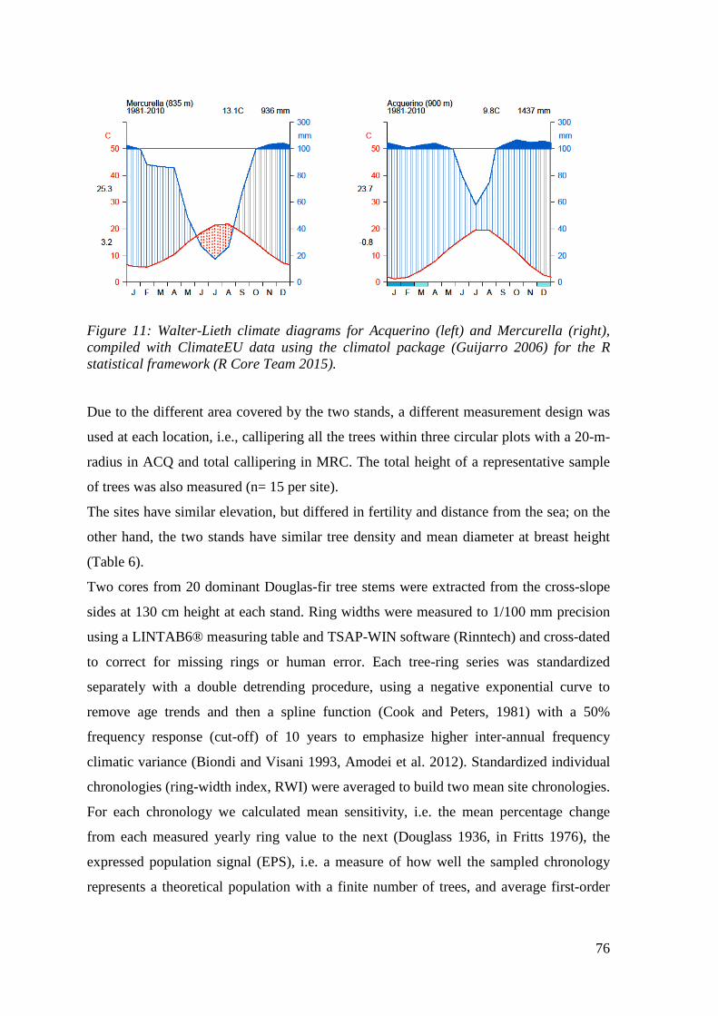
76

Figure 11: Walter-Lieth climate diagrams for Acquerino (left) and Mercurella (right), compiled with ClimateEU data using the climatol package (Guijarro 2006) for the R statistical framework (R Core Team 2015).

Due to the different area covered by the two stands, a different measurement design was

used at each location, i.e., callipering all the trees within three circular plots with a 20-m-

radius in ACQ and total callipering in MRC. The total height of a representative sample

of trees was also measured (n= 15 per site).

The sites have similar elevation, but differed in fertility and distance from the sea; on the

other hand, the two stands have similar tree density and mean diameter at breast height

(Table 6).

Two cores from 20 dominant Douglas-fir tree stems were extracted from the cross-slope

sides at 130 cm height at each stand. Ring widths were measured to 1/100 mm precision

using a LINTAB6® measuring table and TSAP-WIN software (Rinntech) and cross-dated

to correct for missing rings or human error. Each tree-ring series was standardized

separately with a double detrending procedure, using a negative exponential curve to

remove age trends and then a spline function (Cook and Peters, 1981) with a 50%

frequency response (cut-off) of 10 years to emphasize higher inter-annual frequency

climatic variance (Biondi and Visani 1993, Amodei et al. 2012). Standardized individual

chronologies (ring-width index, RWI) were averaged to build two mean site chronologies.

For each chronology we calculated mean sensitivity, i.e. the mean percentage change

from each measured yearly ring value to the next (Douglass 1936, in Fritts 1976), the

expressed population signal (EPS), i.e. a measure of how well the sampled chronology

represents a theoretical population with a finite number of trees, and average first-order

77

autocorrelation (AC), which indicates the influence of the previous year on the current

year’s growth.

Table 6. Main stand (mean value ± standard deviation) and sampled tree characteristics at the two investigated sites.

Acquerino Mercurella

Elevation (m) 900 835

Sea distance (km) 63.8 3.4

Trees (n/ha) 247 294

Basal area (m2) 111.7 90.4

Quadratic mean of tree diameter at 75.9 62.5

Age (years) min 56 60

mean 68 70

max 78 76

Tree height (m) 48.7±5.4 37.5±1.7

Tree diameter at breast height (cm) 69.4±14.8 73.1±8.6

78

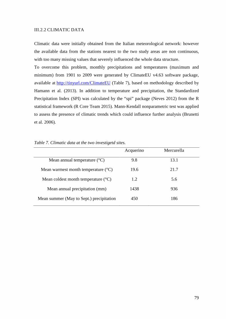
79

III.2.2 CLIMATIC DATA

Climatic data were initially obtained from the Italian meteorological network: however

the available data from the stations nearest to the two study areas are non continuous,

with too many missing values that severely influenced the whole data structure.

To overcome this problem, monthly precipitations and temperatures (maximum and

minimum) from 1901 to 2009 were generated by ClimateEU v4.63 software package,

available at http://tinyurl.com/ClimateEU (Table 7), based on methodology described by

Hamann et al. (2013). In addition to temperature and precipitation, the Standardized

Precipitation Index (SPI) was calculated by the “spi” package (Neves 2012) from the R

statistical framework (R Core Team 2015). Mann-Kendall nonparametric test was applied

to assess the presence of climatic trends which could influence further analysis (Brunetti

et al. 2006).

Table 7. Climatic data at the two investigetd sites.

Acquerino Mercurella

Mean annual temperature (°C) 9.8 13.1

Mean warmest month temperature (°C) 19.6 21.7

Mean coldest month temperature (°C) 1.2 5.6

Mean annual precipitation (mm) 1438 936

Mean summer (May to Sept.) precipitation 450 186

80

81

III.2.3 CLIMATE GROWTH RELATIONSHIPS

The influence of climate on tree-ring growth was investigated using mean correlation

function (CF) and moving correlation functions (MCF), computed on a 30-years-window

to retain the influence of mid-frequency climate variations (Fritts, 1976). This base length

satisfied the conditions (< 80% of all available years; ≥ twice the number of predictors)

suggested by Biondi and Waikul (2004).

Climate variables were calculated at monthly intervals from October of the previous year

(t-1) to September of the year of growth (t). Pearson’s correlations were tested for

significance using the 95% percentile range method after a bootstrap resampling with

1000 replications. The dplR package (Bunn 2008) and the treeclim package (Zang and

Biondi 2015) from R were used for tree ring series management and analysis of climate-

growth relationships.

82

83

III.3 RESULTS

Figure 12: On the left, raw (above) and detrended (below) chronologies of Acquerino stand; on the right, raw (above) and detrended (below) choronologies of Mercurella stand.

In both site chronologies (Figure 12), mean sensitivity was around 12% (table 3) and EPS

was high, indicating that the sampled chronology represents very well the analyzed

populations. After standardization, autocorrelation from carryover effects by previous

year’s growth was mostly canceled out (Table 8).

Table 8. Main tree-ring width chronologies statistical and descriptive parameters for the two investigated sites.

Acquerino Mercurella

Mean sensitivity 0.121 0.127

EPS 0.926 0.913

Autocorrelation (before 0.822 0.918

Autocorrelation (after -0.22 0.218

The Mann-Kendall test ascertained the absence of significant trends in the climate data,

even if a growing linear trend in annual minimum and maximum temperatures was

84

observed for both stands, in particular after 1970 (Figure 13, above). Annual precipitation

decreased in ACQ after 1970, but remained stable in MRC (Figure 4, below).

Figure 13: Climate variables at Acquerino (left) and Mercurella (right) from 1900 to 2015 (thin line: annual data, think line: locally-weighted polynomial regression fit).

Annual SPI did not change in the observation period (1901-2009); both sites exhibited

SPI <0 (i.e., less than median precipitation: McKee et al., 1993) between May-June and

September, and positive winter SPI. ACQ displayed also a spring drought, with increased

frequencies in the last two decades (Figure 14).

Figure 14: Standardized Precipitation Index (SPI) at Acquerino (left) and Mercurella (right) sites.

At ACQ, a significant and positive correlation was found between growth and minimum

and maximum February temperature, whilst a negative correlation was found with

minimum temperature of August-September of the current year and maximum

temperature of July to September of the current year (Figure 15). Precipitation and SPI

were negatively correlated to ring width in October and November of the previous year,

85

and positively correlated in May and July (SPI: May-July-August) of the current year

(Figure 15).

Figure 15: Acquerino stand: above - correlation functions (CF) between ring width and maximum (left) and minimum (right) temperature; below - CF for precipitation (left) and SPI (right).

At MRC, ring width showed a significant and positive correlation with minimum and

maximum temperatures of February and March, and a negative correlation with

maximum temperatures of October (t-1) and July (Figure 16). Precipitation and SPI

showed a negative correlation with ring width in the months of December (t-1) (Figure

16).

86

Figure 16: Mercurella stand: correlation functions (CF) between ring width and maximum (left) and minimum (right) temperature above; CF for precipitation (left) and SPI (right) below.

MCF highlighted several periods with significant Pearson’s correlations between ring

width and climate. While some of them were approximately stable over time, others

appeared unstable throughout the observation period. At ACQ, significant correlations

between ring width and minimum temperatures were generally confirmed across the

whole time-series, even if a significant correlation was also detected for the month of

March in the period 1945-1985 (Figure 17).

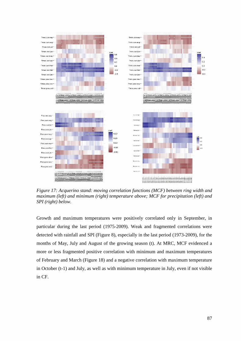
87

Figure 17: Acquerino stand: moving correlation functions (MCF) between ring width and maximum (left) and minimum (right) temperature above; MCF for precipitation (left) and SPI (right) below.

Growth and maximum temperatures were positively correlated only in September, in

particular during the last period (1975-2009). Weak and fragmented correlations were

detected with rainfall and SPI (Figure 8), especially in the last period (1973-2009), for the

months of May, July and August of the growing season (t). At MRC, MCF evidenced a

more or less fragmented positive correlation with minimum and maximum temperatures

of February and March (Figure 18) and a negative correlation with maximum temperature

in October (t-1) and July, as well as with minimum temperature in July, even if not visible

in CF.

88

Figure 18: Mercurella stand: moving correlation functions (MCF) between ring width and maximum (left) and minimum (right) temperature above; MCF for precipitation (left) and SPI (right) below.

89

III.4.DISCUSSION

Minimum temperatures, in particular those of February, are positively correlated with

ring width at both sites; this outlines the preference of this species for the mild climates

and, furthermore, Douglas fir is sensitive to winter frost (Burns and Honkala 1990;

Timmis et al. 1994).

Minimum temperatures of August and September in ACQ are negatively correlated with

growth: the species needs cold temperatures in late summer in order to close the growing

season (sensitivity to early and late frosts). Instead in MRC this correlation was not

significant, because early frosts do not occur due to the greater proximity to the sea.

July temperatures are negatively correlated with growth in MRC (and also in ACQ,

although not significantly), underlying the importance of summer evaporative stress

(Chen et al. 2010). However, summer precipitation (and, more strongly, SPI) were

positively correlated to growth only in ACQ, and not in MRC whose climodiagram

displayed a true summer dry period (Figure 2). This difference can be due either to the

higher continentality of the northern Appennine site, or to differences in physiological

activities of the southernmost population, that may stop growth earlier in the season in

order to adapt to the summer dry period.

Autumn precipitations of the previous year are negatively correlated with growth in both

sites. Similarly, Douglas fire trees on xeric sites on the Alps were previously found to be

sensitive to soil water recharge in the preceding autumn and early spring. Trees on more

mesic sites were more vulnerable to water deficits of shorter duration than on xeric sites

(Lévesque et al. 2013).

The strength and significance of most correlations against temperature, precipitation, and

SPI increased at both sites in the last decades. A shift in the most sensitive month for

summer precipitation and temperature was also observed in ACQ. This may be attributed

to the effect of climate warming; however, as long as winter and spring precipitation

remains sufficient to refill the soil water reservoir, summer growth reductions should not

be too strong even if summers will become drier (Christensen et al., 2007; CH2011,

2011).

Stand and site characteristics may have an influence on the occurrence of water stress

(Bauwe et al. 2012). Carnwath et al. (2012) showed that basal area of Douglas fir was

more sensitive to water availability on xeric sites. There is still much debate as to how

stand density or individual competitive conditions, regulated by initial spacing and

90

thinnings, modify the growth reaction patterns of trees in dry years (e.g., Aussenac and

Granier 1988; Castagneri et al. 2015). On the other hand, more studies are needed to

ascertain the role of soil and stand variables on the climate sensitivity of Douglas fir

planted under Mediterranean mountain environments. This is also a broader key issue for

forest ecosystem monitoring and assessment programs as means of contingently

identifying and assessing mechanisms that influence global changes (Corona 2016).

91

CONCLUSION

Under climate change expectations, Douglas fir is considered to have a great potential to

supplement timber supply in Southern Europe, given its tolerance to summer drought.

Ultimately, this study stresses that growth of Douglas fir in the Italian Apennines is

positively influenced by winter-spring temperature, suggesting a low tolerance of winter

extremes and a need for spring soil water recharge. Summer water stress has a negative

influence only at the site that does not suffer from regular climatic summer drought,

suggesting a possible physiological adaptation of the species.

From a general standpoint, the obtained results highlight the potential of

dendrochronology, and, distinctively, of dendroclimatology, to identify local climatic

adaptations of populations that can normally only be revealed by long-term provenance

trials or genetic analyses (Chen et al. 2010). These results could be extrapolated to the

average environmental conditions of the Mediterranean area, albeit carefulness may be

advised because local populations may be adapted to additional factors other than climate,

such as soils, mycorrhiza, or the pressures of pests and pathogens (Montwè et al. 2015).

This work has calibrated an age-independent, individual-tree, distance-independent

growth and yield simulator for Douglas fir for Central Italy. A tree level simulator is an

effective tool for planning forest management. Calibrating this model to other areas and

for other species in Italian forests may be a useful management support instead of

traditional yield tables.

Other FVS submodels and extensions can be calibrated besides those here considered

(Russell et al. 2015): regeneration, climate-FVS and especially mortality, which is an

important growth submodel to be considered in future evaluations because it is one of the

most sensitive features to changes in future climate regimes, such as increase in drought

severity and duration (Crookston et al. 2010). Simple modifications to the tree mortality

model within PN-FVS could result in improved precision for estimating future number of

trees (e.g., Radtke et al. 2012).

The self-calibration feature of FVS extends the geographic range over which the model

can be exploited, assuming that the factors affecting growth in a given area also affect

growth in the same way elsewhere. If this assumption cannot be accepted, the only other

option is to refit the relationships using data from the geographic area of interest. If this

procedure can be accepted, then the model equations can be calibrated rather easily.

92

Here, we have proved a relevant improvement for the application of FVS in Italy over the

original model. The results also highlight the importance of using long-term historical

growth data for the calibration and validation of the model. Permanent plots are generally

well suited for tracking long-term model reliability and for evaluating model performance

relative to specific treatments. Maintaining existing local networks of permanent plots,

especially those with long histories of measurement, to predict forest growth in the

climate change, is suggested (Crookston et al. 2010).

In conclusion, FVS has been proven to be a suitable type of yield modeling for Douglas

fir forest growth in Italy: (i) it suitably represents current understanding of the dynamic

forest ecosystem and how it responds over time to management interventions; (ii) it

provides a monitoring target to test our assumptions with (for example, stand yield

following different silvicultural treatments and successional pathways when no treatments

are applied); (iii) it provides a modeling framework to integrate existing modeling

components such as crown equations, site index curves and ecological land classification;

(iv) it provides tools to develop and compare various silvicultural treatments; (v)

simulation stand development may be effectively used to inform and instruct forest

managers; (vi) it can be effectively adopted to update inventory data.

93

REFERENCES

Acollalti A (2011). Sviluppo di un modello dinamico ecologico-forestale per foreste a

struttura complessa, PhD Thesis.

Alessandri A, Navarra A (2008). On the coupling between vegetation and rainfall inter-

annual anomalies: possible contributions to seasonal rainfall predictability over

land areas. Geophys. Res. Lett. 35: L02718.

Amodei T, Guibal F, Fady B (2012). Relationships between climate and radial growth in

Black pine (Pinus nigra Arnold ssp. salzmannii (Dunal) Franco) from the south of

France. Annals of Forest Science 70(1): 41-47.

Amorini E, Brandini PG, Fabbio G, Tabacchi G (1998). Modelli di previsione delle masse

legnose e delle biomasse per i cedui di cerro della Toscana centro-meridionale.

Annali dell’istituto Sperimentale per la Selvicoltura 29: 41-56.

Arca B, Duce P, Laconi M, Pellizzaro G, Salis M, Spano D (2007). Evaluation of

FARSITE simulator in mediterranean maquis. International Journal of Wildland

Fire 16: 563-572.

Arney, J.D. (1972). Computer simulation of Douglas-fir tree and stand growth. Ph.D.

Thesis, Oregon State University, Corvallis, OR. 79 p.

Arney, J.D. (1985). A modeling strategy for the growth projection of managed stands.

Canadian Journal of Forest Research 15:511–518.

Attorre F, Francesconi F, Scarnati L, De Sanctis M, Alfò M, Bruno F (2008). Predicting

the effect of climate change on tree species abundance and distribution at a

regional scale. iForest 1: 132-139.

Aussenac G, Granier A (1988). Effects of thinning on water stress and growth in

Douglas-fir. Canadian Journal of Forest Research 18:100-105.

Barber VA, Juday GP, Finney BP (2000) Reduced growth of Alaskan white spruce in the

twentieth century from temperature-induced drought stress. Nature, 405: 668–673.

Bauwe A, Criegee C, Glatzel S, Lennartz B (2012) Model-based analysis of the spatial

variability and long-term trends of soil drought at Scots pine stands in northeastern

Germany. European Journal of Forest Research 131(4): 1013–1024.

Bernetti G, Cantiani M, Hellrigl B (1969). Ricerche alsometriche e dendrometriche sulle

pinete di pino nero e laricio della Toscana. L’Italia Forestale e Montana 44 (1):

10-33.

94

Bertini G, Amoriello T, Fabbio G, Piovosi M, (2011). Forest growth and climate change:

evidences from the ICP-Forests intensive monitoring in Italy. iForest 4: 262-267.

Bianchi M (1981). Le fustaie di faggio di origine agamica della Toscana: tavole di

produzione per i boschi coetanei. Annali Accademia Italiana di Scienze Forestali,

vol. 30, Firenze, Italy.

Biondi F (1997). Evolutionary and moving response functions in dendroclimatology.

Dendrochronologia 15:139-150.

Biondi F (2000). Are climate–tree growth relationships changing in North-Central Idaho,

USA? Arctic Antarctic and Alpine Research 32: 111–116.

Biondi F, Visani S (1993). Cronologie dendroanulari per la Penisola Italiana. Annali della

Facoltà di Agraria, Università Cattolica di Milano, Italia 33 (1): 3-23.

Biondi F, Waikul K (2004). Dendroclim 2002: AC++ program for statistical calibration

of climate signals in tree ring chronology. Computers & Geosciences 30: 303-311.

Bittelli M, Tomei F, Pistocchi A, Flury M, Boll J, Brooks ES, Antolini G (2010).

Development and testing of a physically based, three-dimensional model of

surface and subsurface hydrology. Advances in Water Resources 33: 106-122.

Boisvenue C, Running SW (2006). Impacts of climate change on natural forest

productivity – evidence since the middle of the 20th century. Global Change Biology

12: 862–882.

Boitani L, Corsi F, Falcucci A, Marzetti I, Masi M, Montemaggiori A, Ottavini D,

Reggiani G, Rondinini C (2002). Rete ecologica nazionale. Un approccio alla

conservazione dei vertebrati italiani. Università La Sapienza, Dipartimento di

Biologia Animale e dell’Uomo, Roma, Italy.

Borghetti M, La Mantia T, Menozzi P, Piotti A (2012). Probabili impatti del

cambiamento climatico sulla biodiversità delle foreste italiane. Forest@ 9: 245-250.

Bossel H (1991). Modelling forest dynamics: moving from description to explanation.

Forest Ecology and Management 42: 129-142.

Botkin DB, Janak JF, Wallis JR (1972). Some ecological consequences of a computer

model of forest growth. Journal of Ecology 60: 849-873.

Bouchon J., (1995). Concepts et caractéristiques des divers modèles de croissance. Revue

Forestière Française 47(n° sp.): 23-34.

Bréeda N, Huc R, Granier A, Dreyer E (2006). Temperate forest trees and stands under

severe drought: a review of ecophysiological responses, adaptation processes and

long-term consequences. Annals of Forest Science 63:625–644.

95

Briffa KR, Schweingruber FH, Jones PD, Osborn TJ, Shiyatov SG, Vaganov EA (1998).

Reduced sensitivity of recent tree-growth to temperature at high northern latitudes.

Nature 391: 678–682.

Brugnoli A, Brugnoli R (2006). La foresta come habitat del Gallo cedrone: ricerca

applicata e nuove esperienze di gestione. Forest@ 3: 168-182.

Bruner HD, Moser JW (1973). A Markov chain approach to the prediction of diameter

distributions in uneven-aged forest stands. Canadian Journal of Forest Research 3:

409-417.

Brunetti M, Maugeri M, Monti F, Nanni T (2006). Temperature and precipitation

variability in Italy in the last two centuries from homogenised instrumental time

series. International Journal of Climatology 26: 345–381.

Bugmann H, Palahi M, Bontemps JD, Tome T (2010). Trends in modeling to address

forest management and environmental challenges in Europe: introduction. Forest

Systems 19: 3-7.

Bunn AG (2008). A dendrochronology program library in R (dplR). Dendrochronologia

26(2): 115–124.

Burns RM, Honkala BH (1990). Silvics of North America, Vol. 1, Conifers. Washington

DC: U.S.D.A. Forest Service Agriculture Handbook 654.

Camia A (2009). Storia, sviluppi recenti e applicazioni della previsione del pericolo di

incendio boschivo in Italia. In: “Atti del Terzo Congresso Nazionale di

Selvicoltura per il miglioramento e la conservazione dei boschi italiani” (Ciancio

O ed). Vol. 1, AISF, Firenze, pp. 339-344.

Cantiani MG, Floris A, Tabacchi G (2000). Aspetti produttivi delle peccete altomontane e

subalpine della Val di Fiemme. Comunicazioni di ricerca dell’ISAFA, vol. 3,

Trento, Italy, pp. 3-21.

Cantiani, M. (1965). Tavola alsometrica della Pseudotsuga douglasii in Toscana. Ricerche

sperimentali di dendrometria e auxometria dell’Istituto per l’Assestamento Forestale

dell’Università di Firenze 4:32-73.

Carnwath GC, Peterson DW, Nelson CR (2012). Effect of crown class and habitat type on

climate–growth relationships of ponderosa pine and Douglas-fir. Forest Ecology and

Management 285: 44-52.

Carpenter S (2002). Ecological futures: building an ecology of the long now. Ecology 83:

2069-2083.

96

Carrer M, Nola P, Eduard JL, Motta R, Urbinati C (2007). Regional variability of

climate–growth relationships in Pinus cembra high elevation forests in the Alps.

Journal of Ecology 95: 1072–1083.

Carrer M, Urbinati C (2006). Long-term change in the sensitivity of tree-ring growth to

climate forcing in Larix decidua. New Phytologist 170: 861–871.

Case MJ, Peterson DL (2005). Fine-scale variability in growth-climate relationships of

Douglas-fir, North Cascade Range, Washington. Canadian Journal of Forest

Research 35: 2743-2755.

Castagneri D, Bottero A, Motta R, Vacchiano G (2015). Repeated spring precipitation

shortage alters individual growth patterns in Scots pine forests in the Western Alps.

Trees 29(6): 1699-1712.

Castellani C (1982). Tavole stereometriche ed alsometriche costruite per i boschi italiani.

Istituto Sperimentale per l’Assestamento Forestale e per l’Alpicoltura, Trento.

Cescatti A, Piutti E (1998). Silvicultural alternatives, competition regime and sensitivity

to climate in a European beech forest. Forest Ecology and Management 102(2-3):

213-223.

CH 2011 (2011). Swiss Climate Change Scenarios CH2011. C2SM, MeteoSwiss, ETH,

NCCR Climate, and OcCC, Zurich, Switzerland.

Chen PY, Welsh C, Hamann A (2010) Geographic variation in growth response of

Douglas-fir to interannual climate variability and projected climate change. Global

Change Biology 16: 3374–3385.

Chirici G, Chiesi M, Corona P, Puletti N, Mura M, Maselli F (2015). Prediction of forest

NPP in Italy by the combination of ground and remote sensing data. European

Journal of Forest Research 134: 453-467.

Christensen JH, Hewitson B, Busuioc A et al. (2007). Regional climate projections. In:

Climate Change 2007: The Physical Science Basis. Contribution of Working Group I

to the Fourth Assessment Report of the Intergovernmental Panel on Climate Change,

(eds Solomon S, Qin D, Manning M, Chen Z, Marquis M, Averyt KB, Tignor M,

Miller HL), pp. 847–940. Cambridge University Press, Cambridge, United Kingdom

and New York, NY, USA.

Ciancio O, Nocentini S (2004). Il bosco ceduo. Selvicoltura Assestamento Gestione.

Accademia Italiana di Scienze Forestali, Firenze, Italy.

Ciancio O., Iovino F., Nocentini S., (1994). The theory of normal forest. L’Italia

Forestale e Montana 49(5):446-462.

97

Comeau, P. G., M. White, G. Kerr, and S.E. Hale (2010). Maximum density-size

relationships for Sitka spruce and coastal Douglas-fir in Britain and Canada. Forestry

83(5) :461–468.

Cook ER, Peters K (1981). The smoothing spline: a new approach to standardizing forest

interior tree-ring width series for dendroclimatic studies. Tree-Ring Bulletin 41: 45–

53.

Cook, E.R. and Briffa, K.R., (1990). A comparison of some tree-ring standardization

methods. In: Methods of Dendrochronology (Eds. E.R. Cook and L.A.

Kairiukstis), pp.104-123 Kluwer, Dordrecht.

Coops NC, Waring RH, Landsberg JJ (1998). Assessing forest productivity in Australia

and New Zealand using a physiologically-based model driven with averaged

monthly weather data and satellite-derived estimates of canopy photosynthetic

capacity. Forest Ecology and Management 104: 113-127.

Corona P (2016). Consolidating new paradigms in large-scale monitoring and assessment

of forest ecosystems. Environmental Research 144, 8-14.

Corona P, Marziliano PA, Scotti R (2002). Topdown growth modelling: a prototype for

poplar plantations in Italy. Forest Ecology and Management 161: 65-73.

Corona P, Scotti R (1998). Forest growth-andyield models: questioning support for

sustainable forest management. Journal of Sustainable Forestry 7 (3-4): 131-143.

Corona P, Scotti R, De Paoli M, Tomaiuolo M (1997). DOUG_IT: a growth-and-yield

Java applet for Italian Douglas-fir plantations. In: Proceedings of the IUFRO

Conference “Modelling growth of fast-grown tree species” (Ortega A, Gezan S

eds). Universidad Austral de Chile 5-7. September 1997, pp. 118-126.

Corona, P., R. Scotti, and N. Tarchiani. (1998). Relationship between environmental

factors and site index in Douglas-fir plantations in central Italy. Forest Ecology and

Management 110(1-3):195–207.

Corona P., (1996). Mathematical modelling in forestry: problems and perspectives.

Annali Accademia Italiana di Scienze Forestali, 45: 41-61.

Corona P., (1989). I modelli dendroauxometrici. Monti e Boschi 2: 10-14.

Costantini, E.A.C., G. L’Abate, R. Barbetti, M. Fantappié, R. Lorenzetti, and S. Magini.

2012. Soil map of Italy, scale 1:1.000.000. SELCA, Firenze.

Crookston, N.L. (2005). Allometric crown width equations for 34 Northwest United

States tree species estimated using generalized linear mixed effects models.

98

Manuscript on file with the author at: US Forest Service, 1221South Main St,

Moscow ID, email: ncrookston@fs.fed.us

Crookston, N.L., G.E. Rehfeldt, G.E. Dixon, and A.R. Weiskittel. (2010). Addressing

climate change in the forest vegetation simulator to assess impacts on landscape

forest dynamics. Forest Ecology and Management 260:1198-1211.

Curtis, R.O. (1967). Height-diameter and height-diameter-age equations for second-

growth Douglas-Fir. Forest Science 13 :365–375.

Curtis, R.O., G.W. Clendenen, and D.J. DeMars (1981). A new stand simulator for coast

Douglas-fir: DFSIM user’s guide. USDA For. Serv. Gen. Tech. Rep. PNW-GTR-

128.

Di Filippo A, Biondi F, Cufar K et al. (2007). Bioclimatology of beech (Fagus sylvatica

L.) in the Eastern Alps: spatial and altitudinal climatic signals identified through a

tree-ring network. Journal of Biogeography 34: 1873–1892.

Dixon G.E. (2003). Essential FVS: a user’s guide to the Forest Vegetation Simulator.

Internal Report, Forest Management Service Center, USDA Forest Service, Fort

Collins, CO, USA.

Dixon, G.E. (1985). Crown ratio modeling using stand density index and the Weibull

distribution. USDA For. Serv. Int. Rep.

Dixon, G.E. (1986). Prognosis mortality modeling. USDA For. Serv. Int. Rep.

Dixon, G.E. (2002.) Essential FVS: A User’s Guide. USDA For. Serv. Int. Rep.

Dolph, K.L. (1988). Site index curves for young-growth California white fir on the

western slopes of the Sierra Nevada. USDA For. Serv. Res. Pap. PSW-RP-185.

Dreyfus P, Bonnet FR (1996). CAPSIS (Computer-Aided Projection of Strategies In

Silviculture): an interactive simulation and comparison tool for tree and stand

growth, silvicultural treatments and timber assortment. In: Proceedings of the

Conference on “Connection Between Silviculture and Wood Quality Through

Modelling Approaches and Simulation Softwares” (Nepveu G ed). INRA, Nancy,

France, pp. 194-202.

Ducci F. (2015). Genetic resources and forestry in the Mediterranean region in relation to

global change. Annals of Silvicultural Research 39(2): 70-93.

Eilmann B, Rigling A (2012). Tree-growth analyses to estimate tree species’ drought

tolerance. Tree Physiology 32: 178-187.

99

Eilmann B, Zweifel R, Buchmann N, Fonti P, Rigling A (2009). Drought-induced

adaptation of the xylem in Scots pine and pubescent oak. Tree Physiology 29:1011–

1020.

Eykhoff P (1974). System Identification-Parameter and State Estimation. Wiley, New

York.

Fiorese G, Gatto M, Ranci Ortigosa G, De Leo G (2005). Scenari futuri di impatto dei

cambiamenti climatici globali tramite l’applicazione di modelli di vocazionalità

faunistica a ungulati alpini. In: Atti del XV Congresso Nazionale della Società

Italiana di Ecologia (Comoglio C, Comino E, Bona F eds). Torino (Italy) 12-14

settembre 2005.

Fontes L, Bontemps JD, Bugmann H, Van Oijen M, Gracia C, Kramer K, Lindner M,

Rötzer T, Skovsgaard JP (2010). Models for supporting forest management in a

changing environment. Forest Systems 2010: 8-29.

Forest Europe (2015). State of Europe’s Forests 2015. Madrid, Ministerial Conference on

the Protection of Forests in Europe, Spain.

Franc A, Gourlet-Fleury S, Picard N (2000). Une introduction à la modélisation des forêts

hétérogènes. ENGREF, Nancy, France.

Fritts H.C, (1976). Tree ring and climate. Academic Press, London, UK, pp. 582.

Garcia-Suarez AM, Butler CJ., Baillie MGL (2009). Climate signal in tree-ring

chronologies in a temperate climate: A multi-species approach. Dendrochronologia

27: 183-198.

Gasparini P, Maltoni ML, Tabacchi G (2000). Un modello a matrice di transizione per i

boschi misti pluristratificati di abete rosso, abete bianco e faggio, del Trentino. Vol.

3, Comunicazioni di ricerca ISAFA, Trento, Italy, pp. 23-88.

Guijarro JA (2006). Some Tools for Climatology.

Hamann A, Wang T, Spittlehouse DL, Murdock TQ (2013). A comprehensive, high-

resolution database of historical and projected climate surfaces for western North

America. Bulletin of the American Meteorological Society 94: 1307–1309.

Hamilton, D.A. (1994). Uses and abuses of multipliers in the Stand Prognosis Model.

USDA For. Serv. Gen. Tech. Rep. INT-GTR-310.

Hampe A, Petit RJ (2005). Conserving biodiversity under climate change: The rear edge

matters. Ecology Letters 8: 461– 467.

Hann, D.W., and M.L. Hanus. (2002). Enhanced height-growth-rate for undamaged and

damaged trees in southwest Oregon. Forest Research Lab, Research Contribution 41.

100

Hann, D.W., D.D. Marshall, and M.L. Hanus (2003). Equations for predicting height-to-

crown-base, 5-year diameter-growth rate, 5-year height-growth rate, 5-year mortality

rate, and maximum size-density trajectory for Douglas-fir and western hemlock in

the coastal region of the pacific northwest. Forest Research Lab, Research

Contribution 40.

Hasenauer H (1994). A single tree simulator for uneven-aged mixed species stands. In:

“Mixed Stands: Research Plots, Measurements and Results, Models” (Pinto da

Costa ME, Preuhsler T eds). Instituto superior de Agronomia, Universidad

Técnica de Lisboa, Portugal, pp. 255-270.

He (2008). Forest landscape models: Definitions, characterization, and classification.

Forest Ecology and Management 254: 484-498.

Holdaway, M.R. (1984). Modelling the effect of competition on tree diameter growth as

applied in stems. USDA For. Serv. Gen. Tech. Rep. NC-GTR-94.

Houllier F., Bouchon J., Birot Y., (1991). Modélisation de la dynamique des peuplements

forestieres: état et perspectives. Revue Forestière Française 43: 87-108.

IPCC (2007) Climate change: the physical science basis. In: Contribution of Working

Group I to the Fourth Assessment Report of the Intergovernmental Panel on Climate

Change (eds Solomon S., Qin D., Manning M., Chen Z., Marquis M., Averyt K.B.,

Tignor M., Miller H.L.), Cambridge University Press, Cambridge, UK.

Israel G. (1994). Immagini matematiche della realtà. Le ScienzeQuaderni.

Johnson, N.L., and S. Kotz. (1995). Continuous univariate distributions. New York,

Wiley.

Jørgensen U G. Molecules in Astrophysics: Probes and Processes. (1997). E. F. van

Dishoeck (Kluwer).

Keyser, C.E. (2014). Pacific Northwest Coast (PN) variant overview. USDA For. Serv.

Int. Rep.

Kimmins JP (1993). Scientific foundations for the simulation of ecosystem function and

management in FORCYTE-11. Northwest region. Information Report NOR-X-

328, Forestry Canada, Edmonton, Canada.

Krajicek, J., K. Brinkman, and S. Gingrich (1961). Crown competition-a measure of

density. Forest Science 7(1) :35–42.

Krutchkoff, R.G. (1972). Empirical Bayes estimation. American Statistician 26(5):14-16.

Laneve G, Cadau EG (2007). Quality assessment of the fire hazard forecast based on a

fire potential index for the Mediterranean area by using a MSG/SEVIRI based fire

101

detection system. In: Proceedings of the “IEEE International Geoscience and

Remote Sensing Symposium”. Barcelona (Spain), 23-28 July 2007, pp. 2447-

2450.

Laurent M, Antoine N, Joel G (2003). Effects of different thinning intensities on drought

response in Norway spruce (Picea abies (L.) Karst.). Forest Ecology and

Management 183:47–60.

Ledig FT, Kitzmiller JH (1992). Genetic strategies for reforestation in the face of global

climate change. Forest Ecology and Management 50: 153–169.

Leemans R, Prentice IC (1989). FORSKA, a general forest succession model. Institute of

Ecological Botany, Uppsala, Sweden.

Lipow SR, Johnson GR, St Clair JB, Jayawickrama KJ (2003). The role of tree

improvement programs for ex situ gene conservation of coastal Douglas-fir in the

Pacific Northwest. Forest Genetics 10: 111–120.

Lipow SR, Vance-Borland K, St Clair JB, Henderson J, McCain C (2004). Gap analysis

of conserved genetic resources for forest trees. Conservation Biology 18: 412–423.

Maetzke, F., and S. Nocentini (1994). Dominant-height growth and site index curves for

Douglas fir. Italia Forestale e Montana 49:582–594.

Marletto V, Zinoni F, Filippi N, Angelelli AM Laruccia N, Lega P, Tonelli T (1993).

CRITERIA: an integrated geo-graphical system for soil water monitoring. In:

Proceedings of the “IX Symposium on Pesticide Chemistry, Mobility and

Degradation of Xenobiotics” (Del Re AAM, Capri E, Evans SP, Natali P,

Trevisan MP eds). Piacenza (Italy) 12-13 october 1993, pp. 695-706.

Maselli F, Chiesi M, Barbati A, Corona P (2010). Assessment of forest net primary

production through the elaboration of multisource ground and remote sensing data.

Journal of Environmental Monitoring 12:1082–1091.

Matyas C (1994). Modeling climate-change effects with provenance test data. Tree

Physiology 14: 797–804.

McArdle, R.E., W.H. Meyer, and D. Bruce (1949). The yield of Douglas-fir in the Pacific

Northwest. USDA For. Serv. Tech. Bull. 201.

McKee TB, Doesken NJ, Kleist J (1993). The relationship of drought frequency and

duration of time scales. Eighth Conference on Applied Climatology, American

Meteorological Society, Jan17-23, Anaheim CA, pp.179-186.

Mitchell, K.J. (1975). Dynamics and simulated yield of Douglas-fir. Forest Science

Monograph 17:1-39.

102

Monserud RA (2003). Evaluating forest models in a sustainable forest management

context. Forest Biometry, Modelling and Information Sciences 1: 35-47.

Monserud, R.A, and H. Sterba (1996). A basal area increment model for individual trees

growing in even- and uneven-aged forest stands in Austria. Forest Ecology and

Management 80:57–80.

Montwé D, Spiecker H, Hamann A (2015). Five decades of growth in a genetic field trial

of Douglas-fir reveal trade-offs between productivity and drought tolerance. Tree

Genetics & Genomes 11: 29.

Monty, A., P. Lejeune, and J. Rondeux (2008). Individual distance-independent girth

increment model for Douglas-fir in southern Belgium. Ecological Modelling 212(3-

4):472–479.

Morani A (2009). Optimizing tree planting in New York city. Tesi di laurea di secondo

livello, Università della Tuscia, Facoltà di Agraria, Viterbo, Italy.

Munro D (1974). Forest growth models: a prognosis. In: Proceedings of “Growth models

for tree and stand simulation” (Fries J eds). Royal College of Forestry, Stockholm,

Sweden, pp. 7-21.

Neves J (2015). Compute the SPI index using R®.

Newnham, R.M., and J. H. G. Smith (1964). Development and testing of stand models for

douglas fir and lodgepole pine. The Forestry Chronicle 40:494-504.

Nocentini, S. (2010). Le specie forestali esotiche: la sperimentazione di Aldo Pavari e le

prospettive attuali. Italia Forestale e Montana 65(4):449–457.

Nolé A, Law BE, Magnani F, Matteucci G, Ripullone F, Borghetti M (2009). Application

of the 3-PGs model to assess carbon accumulation in forest ecosystems at a

regional level. Canadian Journal of Forest Research 3 (9): 1647-1661.

Ottorini, J. (1991). Growth and development of individual Douglas-fir in stands for

applications to simulate silviculture. Annals of Forest Science 48(6):651–666.

Pacala SW, Canham CD, Silander J (1993). Forest models defined by field

measurements: I. The design of a northeastern forest simulator. Canadian Journal

of Forest Research 23: 1980-1988.

Paine, D.P, and D.W. Hann (1982). Maximum crown-width equations for Southwestern

Oregon tree species. Oregon State University, Forest Research Lab, Research

Contribution 46.

Palahí M (2008). Forest models for research and decision support in sustainable forest

management. WG1: Summary of the information from the country templates.

103

Pavari A (1958). La Douglasia verde in Italia. Monti e Boschi 9: 42–58.

Pavari A, De Philippis A (1941). La sperimentazione di specie forestali esotiche in Italia.

Risultati del primo ventennio. Annali della Sperimentazione Agraria, vol. 38. Failli,

Roma.

Pavari, A. (1916). Studio preliminare sulle colture di specie forestali esotiche in Italia.

Annali del Regio Istituto Superiore Forestale Nazionale 1:159-379.

Pellizzari, E., Pividori, M., Carrer, M. (2014). Winter precipitation effect in a mid-latitude

temperature-limited environment: the case of common juniper at high elevation in

the Alps. Environmental Research Letters, 9: 1-9.

Peng C (2000). Growth and yield models for uneven-aged stands: past, present and future.

Forest Ecology and Management 132: 259-279.

Pickett STA, Kolasa J (1989). Structure of theory in vegetation science. Plant Ecology 83:

7-15.

Porté A, Bartelink HH (2002). Modelling mixed forest growth: a review of models for

forest management. Ecological Modelling 150: 141-188.

Pretzsch H (1999). Modelling growth in pure and mixed stands: a historical overview. In:

“Management of mixed-species forest: silviculture and economics” (Olsthoorn

AFM, Bartelink HH, Gardiner JJ, Pretzsch H, Hekhuis HJ, Franc A, Wall S eds).

Instituut voor Bos- en Natuuronderzoek DLO, Wageningen, The Netherlands, pp.

102-107.

Pretzsch H, Biber P, Dursky J, Gadow K, Hasenauer H, Kändler G, Kenk G, Kublin E,

Nagel J, Pukkala T, Skovsgaard J, Sodtke R, Sterba H (2006). Standardizing and

categorizing tree growth models. In: “Sustainable Forest Management: growth

models for Europe” (Hasenauer Hed). Springer, Berlin, Germany, pp. 39-57.

Pretzsch H, Grote R, Reineking B, Rotzer T, Seifert S (2008). Models for forest

ecosystem management: a European perspective. Annals of Botany 101: 1065-

1087.

Pretzsch H, Kahn M (1996). Wuchsmodelle für die Unterstützung der Wirtschaftsplanung

im Forstbetrieb. Allgemeine Forst Zeitschrift Der Wald 25: 1414-1419.

Pretzsch, H. (2009). Forest dynamics, growth and yield. Berlin, Springer.

Pretzsch, H., and P. Biber (2005). A re-evaluation of Reineke’s rule and stand density

index. Forest Science 51(4):304–320.

Pucci, A. 1882. Le conifere di Moncioni. Firenze, Ricci.

104

R Core Team (2015). R: A language and environment for statistical computing. R

Foundation for Statistical Computing, Vienna, Austria. URL http://www.R-

project.org/.

Radtke, P.J., N.D. Herring, D.L. Loftis, and C.E. Keyser. (2012). Evaluating Forest

Vegetation Simulator predictions for southern Appalachian upland hardwoods with a

modified mortality model. Southern Journal of Applied Forestry 36(2):61-70.

Rais A, Kuilen JW, Pretzsch H (2014). Growth reaction patterns of tree height, diameter,

and volume of Douglas-fir (Pseudotsuga menziesii [Mirb.] Franco) under acute

drought stress in Southern Germany. European Journal of Forest Research 133:

1043-1056.

Rebetez M, Mayer H, Dupont O, Schindler D, Gartner K et al. (2003). Heat and drought

2003 in Europe: a climate synthesis. Annals of Forest Science, Springer Verlag/EDP

Sciences, 2006, 63 (6): 569-577.

Regional Forest Inventory of Tuscany (1998). L’inventario forestale. Firenze, Regione

Toscana.

Rehfeldt GE, Ying CC, Spittlehouse DL, Hamilton DA (1999). Genetic responses to

climate in Pinus contorta: niche breadth, climate change, and reforestation.

Ecological Monographs 69: 375–407.

Rehman, S. (1999). Empirical model development and comparison with existing

correlations. Applied Energy 64:369–378.

Reineke, L.H. (1933). Perfecting a stand-density index for even-aged forests. Journal of

Agricultural Research 46(7):627–638.

Rigling A, Bräker O, Schneiter G, Schweingruber F (2002). Intraannual tree-ring

parameters indicating differences in drought stress of Pinus sylvestris forests within

Erico-Pinion in Valais (Switzerland). Plant Ecology 163: 105–121.

Rigon R, Bertoldi G, Over TM (2006). GEOtop: a distributed hydrological model with

coupled water and energy budgets. Journal of Hydrometeorology 7: 371-388.

Ritchie, M.W., and D.W. Hann. (1985). Equations for predicting basal area increment in

Douglas-fir and grand fir. Oregon State University, Forest Research Lab, Research

Contribution 4.

Ruiz Diaz Britez, M., A.S Sergent, A. Martinez Meier, N. Bréda, and P. Rozenberg

(2014). Wood density proxies of adaptive traits linked with resistance to drought in

Douglas fir (Pseudotsuga menziesii (Mirb.) Franco). Trees 28(5):1289-1304.

105

Russell, M.B., A.R. Weiskittel, and J.A. Kershaw (2013). Benchmarking and calibration

of Forest Vegetation Simulator individual tree attribute predictions across the

northeastern United States. Northern Journal of Applied Forestry 30(2):75-84.

Russell, M.B., A.W. D'Amato, M.A. Albers, C.W. Woodall, K.J. Puettmann, M.R.

Saunders, and C.L. VanderSchaaf (2015). Performance of the Forest Vegetation

Simulator in managed white spruce plantations influenced by eastern spruce

budworm in northern Minnesota. Forest Science 61(4):723-730.

Schar C, Vidale PL, Luthi D, Frei C, Haberli C, Liniger MA, Appenzeller C (2004). The

role of increasing temperature variability in European summer heatwaves. Nature

427: 332-336.

Schmid, M., M. Pautasso, and O. Holdenrieder (2014). Ecological consequences of

Douglas fir (Pseudotsuga menziesii) cultivation in Europe. European Journal of

Forest Research 133(1):13–29.

Schweingruber FH, (2007). Wood Structure and Environment. Springer, ISBN: 1431-

8563.

Schweingruber FH. (1988). Tree rings - basics and applications of dendrochronology.

Kluwer Academic Publishers. ISBN 90277244 58. 276 pages.

Scotti R, Corona P, La Marca O, Marziliano PA, Tarchiani N, Tomaiuolo M (1995).

Growth model for italian douglas-fir plantations. In: “Recent advances in forest

mensuration and growth and yield research”. Proceedings from 3 sessions of

Subject Group S4.01 “Mensuration, Growth and Yield”, 20th World Congress of

IUFRO (Skovsgaard JP, Burkhart HE eds). Tampere (Finland) 6-12 August 1995.

Finnish Forest and Landscape Research Institute, Tampere, Finland, pp. 175-193.

Seager R, Ting MF, Held I et al. (2007). Model projections of an imminent transition to a

more arid climate in southwestern North America. Science 316: 1181–1184.

Sergent AS, Rozenberg P, Bréeda N (2012). Douglas-fir is vulnerable to exceptional and

recurrent drought episodes and recovers less well on less fertile sites. Annals of

Forest Science 71: 697-708.

Sergent, A.S., N. Bréda, L. Sanchez, J.C. Bastein, and P. Rozenberg. (2014a). Coastal and

interior Douglas-fir provenances differ in growth performance and response to

drought episodes at adult age. Annals of Forest Science 71(6) :709-720.

Sergent, A.S., P. Rozenberg, and N. Bréda. (2014b). Douglas-fir is vulnerable to

exceptional and recurrent drought episodes and recovers less well on less fertile

sites. Annals of Forest Science 71(6):697-708.

106

Shaw J.D., G. Vacchiano, R.J. DeRose, A. Brough, A. Kusbach, and J.N. Long (2006).

Local calibration of the Forest Vegetation Simulator (FVS) using custom inventory

data. In Proceedings of the 2006 Society of American Foresters National Convention,

Pittsburgh PA, October 25-29, 2006. Society of American Foresters, Bethesda, MD.

Shaw, J.D. (2006). Reineke’s Stand Density Index: where are we and where do we go

from here? In Proceedings of the Society of American Foresters 2005 National

Convention, October 19-23 2005, Ft. Worth, TX.

Shugart HH (1984). A theory of forest dynamics: the ecological implications of forest

succession models. Springer, New York, USA.

Shugart HH, Michaels PJ, Smith TM, Weinstein DA, Rastetter EB (1988). Simulation

Models of Forest Succession. In: “Scales and global change: spatial and temporal

variability in biospheric and geospheric processes” (Rosswall T, Woodmansee

RG, Risser PG eds). John Wiley and Sons, Chichester, USA, pp. 125-151.

Siipilehto, J., S. Sarkkola, and L. Mehtatalo. (2007). Comparing regression estimation

techniques when predicting diameter distributions of Scots pine on drained peatlands.

Silva Fennica 41:333–349.

Sohn JA, Kohler M, Gessler A, Bauhus J (2012). Interactions of thinning and stem height

on the drought response of radial stem growth and isotopic composition of Norway

spruce (Picea abies). Tree Physiology 32:1199–1213.

Spiecker H (2010). Opportunities and risks for Douglas fir in a changing climate -

Abstracts. Berichte Freiburger Forstliche Forschung 85:65.

St Clair JB, Howe GT (2007). Genetic maladaptation of coastal Douglas-fir seedlings to

future climates. Global Change Biology 13: 1441–1454.

Stage AR (1973). Prognosis model for stand development. Research Paper INT-137,

Intermountain Forest and Range Experiment Station, USDA Forest Service,

Ogden, UT, USA.

Stage, A. (1981). Use of self calibration procedures to adjust general regional yield

models to local conditions. P. 365-375 in Proceedings of the XVII IUFRO World

Congress 5.4.01, Sept. 6-17, Niigata, Japan.

Sterba H (1981). Radial increment along the bole of trees: problems of measurement and

interpretation. Dickenwachstum der Baume— radial growth trees—la croissance des

arbres en diametre. IUFRO proceedings: physiological aspects of forest ecology

Mitteilungen der Forstlichen Bundesversuchsanstalt Wien: 67–74.

107

Taylor AR, Chen HYH, VanDamme L (2009). A review of forest succession models and

their suitability for forest management planning. Forest Science 55: 23-36.

Tessier, L. (1984). Dendroclimatologie et écologie de Pinus sylvestris L. et Quercus

pubescens Wild dans le Sud-Est d-el la France. Thèse de Docteur en Sciences.

Univ. Aix-Marseille III, Fac. St. Jerome, Marseille.

Timmis R, Flewelling J, Talbert C (1994). Frost injury prediction model for Douglas-fir

seedlings in the Pacific Northwest. Tree Physiology 14: 855-869.

Vacchiano G., J.D. Shaw, R.J. DeRose and J.N. Long (2008). Inventory-based sensitivity

analysis of the large tree diameter growth submodel of the Southern Variant of FVS.

P. 149-169 in Proceedings of the Third Forest Vegetation Simulator Conference; Fort

Collins, February 13–15, 2007, Havis R.N., and N.L. Crookston (eds.). USDA Forest

Service, Fort Collins, CO.

Vacchiano, G., E. Lingua, and R. Motta (2005). Valutazione dello Stand Density Index in

popolamenti di abete bianco (Abies alba Mill.) nel Piemonte meridionale. Italia

Forestale e Montana 60(3):269–286.

Vacchiano, G., R. Motta, G. Bovio, and D. Ascoli (2014). Calibrating and testing the

forest vegetation simulator to simulate tree encroachment and control measures for

heathland restoration in Southern Europe. Forest Science 60(2):241-252.

Van der Maaten, E (2012). Climate sensitivity of radial growth in European beech (Fagus

sylvatica L.) at different aspects in southwestern Germany. Trees - Structure and

Function, 26 (3): 777–788.

Van Dyck, M.G., and E.E. Smith-Mateja (2000). Keyword reference guide for the Forest

Vegetation Simulator. USDA For. Serv. Int. Rep.

Van Mantgem PJ, Stephenson NL, Byrne JC et al. (2009). Widespread increase of tree

mortality rates in the Western United States. Science 323: 521–524.

Vanclay J (1994). Modelling forest growth and yield: applications to mixed tropical

forests. CAB International, Wallingford, USA.

Ventura F, Marletto V, Zinoni F (2001). Un metodo per il calcolo dell’indice

meteorologico del rischio di incendio forestale. Sherwood 68: 13-18.

Virgilietti P, Buongiorno J (1997). Modeling forest growth with management data: a

matrix approach for the Italian Alps. Silva Fennica 31: 27-42.

Weber P, Bugmann H, Rigling A (2007). Radial growth responses to drought of Pinus

sylvestris and Quercus pubescens in an inner-Alpine dry valley. Journal of

Vegetation Science 18: 777–792.

108

Wensel, L.C., W.J. Meerschaert, and G.S. Biging (1987). Tree height and diameter

growth models for Northern California conifers. Hilgardia 55(8):1-18.

Wimberly, M.C., and B.B. Bare (1996). Distance-dependent and distance-independent

models of douglas-fir and western hemlock basal area growth following silvicultural

treatment. Forest Ecology and Management 89(1-3):1–11.

Wykoff, R.W., N.L Crookston, and A.R. Stage (1982). User ’s guide to the Stand

Prognosis Model. USDA For. Serv. Gen. Tech. Rep. INT-GTR-122.

Wykoff, W.R. (1986). Supplement to the User’s Guide for the Stand Prognosis Model —

Version 5.0. USDA For. Serv. Gen. Tech. Rep. INT-GTR-208.

Wykoff, W.R. (1990). A basal area increment model for individual conifers in the

northern Rocky Mountains. Forest Science 36(4):1077–1104.

Yoda, K., T. Kira, H. Ogawa, and K. Hozumi (1963). Intraspecific competition among

higher plants. XI. Self-thinning in overcrowded pure stands under cultivated and

natural conditions. Journal of the Institute of Polytechnics of the Osaka City

University 14:107–129.

Zang C, Biondi F (2015). “treeclim: an R package for the numerical calibration of proxy-

climate relationships.” Ecography 38(4): 431-436.