1

Color Demosaicking via Directional Linear Minimum Mean

Square-Error Estimation

Lei Zhang and Xiaolin Wu*, Senior Member, IEEE

Dept. of Electrical and Computer Engineering, McMaster University

Email: {johnray, xwu}@mail.ece.mcmaster.ca

Abstract-- Digital color cameras sample scenes using a color filter array of mosaic pattern (e.g. the

Bayer pattern). The demosaicking of the color samples is critical to the quality of digital

photography. This paper presents a new color demosaicking technique of optimal directional

filtering of the green-red and green-blue difference signals. Under the assumption that the primary

difference signals (PDS) between the green and red/blue channels are low-pass, the missing green

samples are adaptively estimated in both horizontal and vertical directions by the linear minimum

mean square-error estimation (LMMSE) technique. These directional estimates are then optimally

fused to further improve the green estimates. Finally, guided by the demosaicked full-resolution

green channel, the other two color channels are reconstructed from the LMMSE filtered and fused

PDS. The experimental results show that the presented color demosaicking technique significantly

outperforms the existing methods both in PSNR measure and visual perception.

Index Terms: Color demosaicking, Bayer color filter array, LMMSE, directional filtering.

EDICS: 4-COLR, 2-COLO.

*Corresponding author: the Department of Electrical and Computer Engineering, McMaster University, 1280 Main Street West, Hamilton, Ontario, Canada, L8S 4L8. Email: xwu@mail.ece.mcmaster.ca. Tel: 1-905-5259140, ext 24190. This research is supported by Natural Sciences and Engineering Research Council of Canada Grants: IRCPJ 283011-01 and RGP45978-2000.

2

I. Introduction

Most digital cameras capture an image with a single sensor array. At each pixel, only one of the

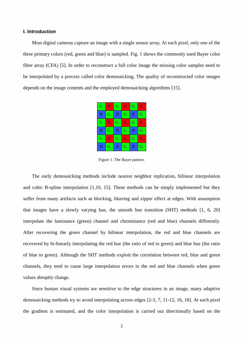
three primary colors (red, green and blue) is sampled. Fig. 1 shows the commonly used Bayer color

filter array (CFA) [5]. In order to reconstruct a full color image the missing color samples need to

be interpolated by a process called color demosaicking. The quality of reconstructed color images

depends on the image contents and the employed demosaicking algorithms [15].

Figure 1. The Bayer pattern.

The early demosaicking methods include nearest neighbor replication, bilinear interpolation

and cubic B-spline interpolation [1,10, 15]. These methods can be simply implemented but they

suffer from many artifacts such as blocking, blurring and zipper effect at edges. With assumption

that images have a slowly varying hue, the smooth hue transition (SHT) methods [1, 6, 20]

interpolate the luminance (green) channel and chrominance (red and blue) channels differently.

After recovering the green channel by bilinear interpolation, the red and blue channels are

recovered by bi-linearly interpolating the red hue (the ratio of red to green) and blue hue (the ratio

of blue to green). Although the SHT methods exploit the correlation between red, blue and green

channels, they tend to cause large interpolation errors in the red and blue channels when green

values abruptly change.

Since human visual systems are sensitive to the edge structures in an image, many adaptive

demosaicking methods try to avoid interpolating across edges [2-3, 7, 11-12, 16, 18]. At each pixel

the gradient is estimated, and the color interpolation is carried out directionally based on the

G

G

R

B

G

G

R

B

G

G

R

B

G

G

R

B

G

G

R

B

G

G

R

B

G

G

R

B

G

G

R

B

G

G

R

B

3

estimated gradient. Directional filtering is the most popular approach for color demosaicking that

produces competitive results in the literature. The best known directional interpolation scheme is

perhaps the second order Laplacian filter proposed by Hamilton and Adams [2-3, 11]. They used the

second order gradients of blue and red channels as the correction terms to interpolate the green

channel. The smaller of the two second order gradients in the horizontal and vertical directions is

added to the average of the green samples along the chosen direction. Once the green samples are

filled, the red and blue samples are interpolated similarly with the correction of the second order

gradients of the green channel. Chang et al. [7] proposed a more complicated gradient-based

demosaicking scheme. They computed a set of gradients in different directions in the 55×

neighborhood centered at the pixel to be interpolated. A subset of these gradients is selected by

adaptive threshold. At last the missing samples are estimated from the known samples located along

the selected gradients. Recently, Ramanath and Snyder [18] proposed a bilateral filtering based

scheme to denoise, sharpen and demosaick the image simultaneously. Alleysson et al. [4] wrote a

color pixel as the sum of luminance and chrominance, and reconstructed the image by selecting the

luminance and chrominance components in Fourier domain.

Another class of color demosaicking techniques is iterative schemes, which can also be

combined with gradient-based methods. Kimmel developed a two-step iterative demosaicking

process consisting of a reconstruction step and an enhancement step [13]. He calculated eight

directional derivatives at each pixel based on its eight neighbors. Based on these edge indicators,

the hue values are computed and the missing green, red and blue samples are then corrected

iteratively by the ratio rule. Finally, an inverse color diffusion process is applied to the whole image

for enhancement. Another iterative demosaicking scheme was proposed by Gunturk et al. [9].

Exploiting the fact that the three color channels of a natural image are highly correlated, Gunturk et

al. reconstructed the color images by projecting the initial estimates onto so-called constraint sets.

They first interpolated the image using Bilinear or other demosaicking methods, and then updated

4

the green channel by the high frequency information of red and blue channels. At last a wavelet-

based iterative process was employed to update the high frequency details of the red and blue

channels according to the green channel. Other demosaicking methods were also proposed, such as

minimum mean square-error estimation [19], pattern matching [21], and median filtering [8].

In all color demosaicking techniques gradient analysis plays a central role in reconstructing

sharp edges. However, the gradient estimate may not be robust when the input signal exceeds the

Nyquist frequency. This is the main cause of color artifacts in demosaicked images. The challenge

is to use statistically valid constraints to overcome the limit of Nyquist frequency. A common

practice in color demosaicking is to exploit the correlation between the color channels. Since the

three color channels of a natural image are highly correlated, the difference signal between the

green channel and the red or blue channel constitutes a smooth (low-pass) process. Furthermore, we

observe that this color difference signal is largely uncorrelated to the interpolation errors of

gradient-guided color demosaicking methods, which are basically band-pass processes. These

observations provide a rationale for estimating the color difference signals by linear minimum mean

square-error estimation (LMMSE) method, which yields a good approximation to the optimal

estimation in mean square-error sense. The LMMSE estimates are obtained in both horizontal and

vertical directions, and then fused optimally to remove the demosaicking noise. Finally, the full-

resolution three color channels are reconstructed from the LMMSE filtered difference signals. The

experimental results show that the new color demosaicking technique significantly outperforms the

state-of-the-art methods both in PSNR measure and visual perception.

This paper is structured as follows. In Section II we introduce the notions of primary difference

signal (PDS) and the directional demosaicing noises. Section III presents the LMMSE technique of

estimating primary difference signals in both horizontal and vertical directions. Section IV describes

how these two directional estimates can be optimally fused into a more robust estimate. Then in

Section V the chrominance channels are interpolated based on the estimated PDS and luminance

5

channel. Section VI gives the experimental results and Section VII concludes.

II. Primary Difference Signal and Directional Demosaicing Noise

Table 1. The correlation coefficients of all pairs of primary color channels. crg is the correlation coefficient of green and red channels; cbg is the correlation coefficient of green and blue channels; and crb is the correlation coefficient of red and blue channels.

Images 1 2 3 4 5 6 7 8 9 crg .9871 .9284 .9726 .9746 .9947 .9976 .9796 .9965 .9790 cbg .9878 .9891 .9803 .9713 .9985 .9928 .9980 .9821 .9569 crb .9540 .9243 .9346 .9492 .9921 .9837 .9711 .9760 .9335

Images 10 11 12 13 14 15 16 17 18 crg .9952 .9955 .9952 .9693 .9991 .9951 .9924 .9929 .9823 cbg .9910 .9892 .9967 .9942 .9921 .9854 .9940 .9965 .9823 crb .9845 .9785 .9884 .9589 .9873 .9694 .9834 .9871 .9629

In order for a color demosaicking algorithm to recover high frequency features beyond the

designed Nyquist frequency of the CFA, it has to rely on some additional statistical property or

constraint(s) about the input color signals. A commonly exploited property is the correlation

between the sampled primary color channels: red, green, and blue. In order to utilize this property in

demosaicking, let us examine the relationships between the green and red channels, and between the

green and blue channels. There are multiple reasons for why the green channel plays a key role in

our estimation of missing color samples. First, the green channel has twice as many samples as the

other two channels in the ubiquitous Bayer mosaic pattern, which is by far the prevailing CCD

sensor design. Second, the sensitivity of the human visual system peaks at the green wavelength.

Third, the green is closer to red and to blue than the difference between red and blue in wavelength.

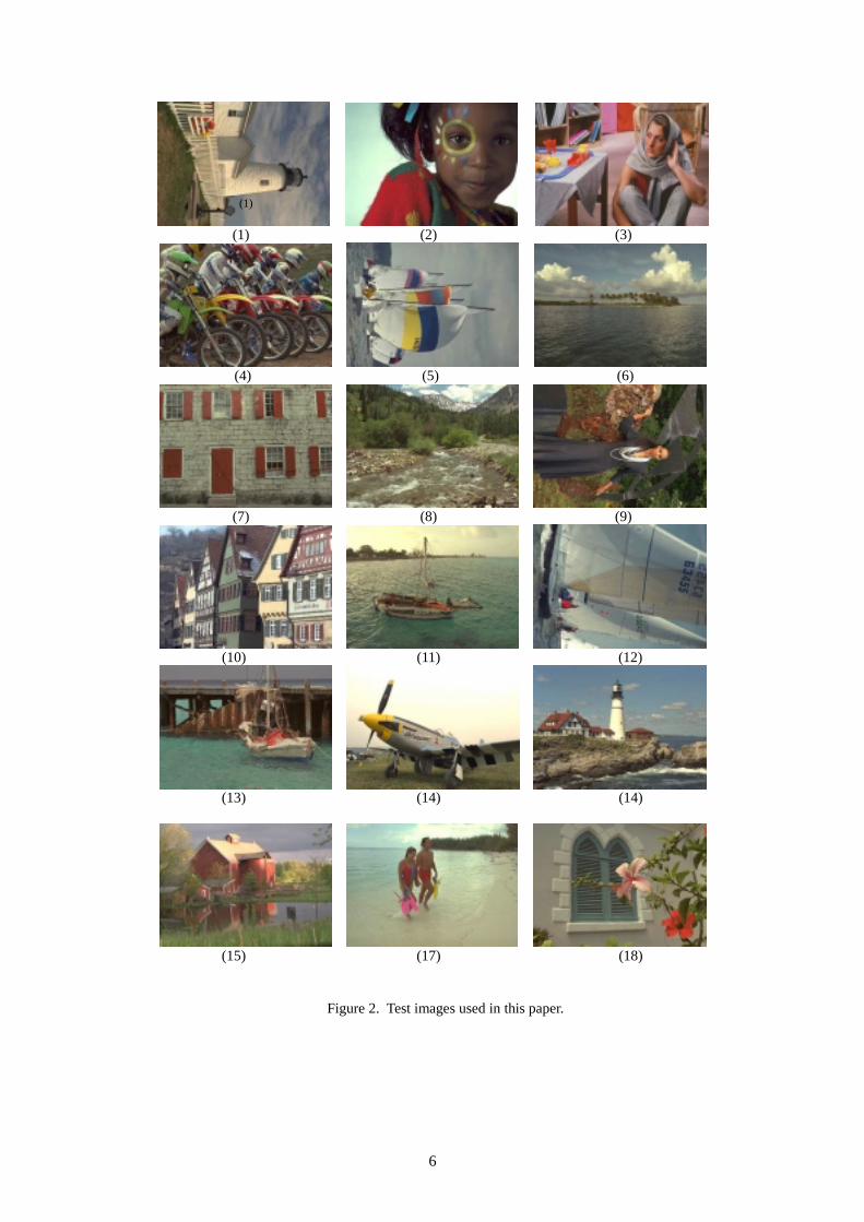
Table 1 lists the average correlation coefficients between all pairs of primary color channels

measured over a set of 18 color test images shown in Fig.2. Clearly, the green-red and green-blue

correlations are appreciably and consistently greater than the red-blue correlation.

6

(1) (2) (3)

(4) (5) (6)

(7) (8) (9)

(10) (11) (12)

(13) (14) (14)

(15) (17) (18)

Figure 2. Test images used in this paper.

(1)

7

In the color demosaicking literature, two assumptions were made on green-red and green-blue

relations: equal ratio [1, 6, 13, 20] and equal difference [2-3, 7, 11]. The former assumption holds

for mosaic CCD data prior to gamma correction, while the latter assumption is closer to the reality

for gamma corrected mosaic CCD data. In this paper, we assume the difference images between the

green and red channels, and between the green and blue channels to be low-pass signals, which are

referred in the sequel as primary difference signals (PDS), and denoted by (referring to Fig. 1)

nnrg n RG)(, −=∆ ; nnbg n BG)(, −=∆ (2-1)

where n is the position index of the pixels. The term is used because (2-1) represents two images

whose pixel values are differences between corresponding green and red/blue samples.

For all reasons above, we demosaick the green channel first and then other two channels as

many other researchers. Namely, we estimate the missing green samples under the assumption that

rg ,∆ and bg ,∆ are smooth signals (some power spectrum density functions of rg ,∆ and bg ,∆ are

plotted in Section III to support this assumption). The quality of final full color reconstruction

largely hinges on the estimation accuracy of the missing green samples in the Bayer pattern,

because the reconstructed green channel has an anchor affect on subsequent steps of demosaicing

the red and blue channels as we will see in Section V. We estimate PDS rg ,∆ and bg ,∆ rather than

individual color channels directly because random processes rg ,∆ and bg ,∆ have some statistical

properties that can be exploited to aid demosaicking. In particular, we are interested in how the

demosaicking noise relates to rg ,∆ and bg ,∆ .

One of the well known and most effective color demosaicking filters is the second-order

directional Laplacian filter of Adams and Hamilton [2-3, 11], which is also based on the assumption

that rg ,∆ and bg ,∆ are constant in either horizontal or vertical direction. The key component of most

existing adaptive demosaicing algorithms is the selection of the direction of color interpolation. In

this paper, however, we make two separate estimates of a missing primary color sample in both

8

horizontal and vertical directions, and then optimally combine the two estimates (the topics of

Sections III and IV).

Figure 3. A row and a column of mosaic data that intersect at a red sampling position.

For concreteness and without loss of generality, we examine the configuration of the Bayer

pattern as shown in Fig. 3: a column and a row of alternating green and red samples intersect at a

red sampling position where the missing green value needs to be estimated. The results for the

symmetric case of estimating the missing green values at the blue sampling positions of the Bayer

pattern can be derived in the same way. We denote the red sample at the center of the window as

0R . Its interlaced red and green neighbors in horizontal direction are labeled as hiR ,

{ }�� ,4,2,2,4, −−∈i , and hiG , { }�� ,3,1,1,3, −−∈i respectively; similarly, the red and green

neighbors of 0R in vertical direction are vjR , { }�� 4,2,2,4, −−∈j , and v

jG , { }�� ,3,1,1,3, −−∈j

respectively. The sample 0R at the intersection can be taken as h0R or v

0R freely.

To get some coarse measurements of PDS rg ,∆ and bg ,∆ , we first interpolate the missing green

samples at red and blue pixels and then interpolate the missing red and blue samples at green

samples. Any of the existed interpolation methods for color demosaicking [2-4, 6-9, 12-13, 16, 18]

may be used. We adopt the second-order Laplacian interpolation filter for its easy implementation

0R

v2-R

v4-R

v1-G

v3-G

v4R

v2Rv3G

v1G

h2-Rh

4-R h1-Gh

3-G h4Rh

2R h3Gh

1G

9

and good performance. (But we stress that the following development is independent of the

interpolation methods.) For any red original sample hiR or v

jR , the corresponding missing green

sample is interpolated as

( ) ( )hi

hi

hi

hi

hi

hi 2211 RRR2

41GG

21G +−+− −−⋅++= (2-2)

( ) ( )vj

vj

vj

vj

vj

vj 2211 RRR2

41GG

21G +−+− −−⋅++= (2-3)

Similarly, for any original green sample hiG or v

jG , the corresponding missing red sample is

interpolated as

( ) ( )hi

hi

hi

hi

hi

hi 2211 GGG2

41RR

21R +−+− −−⋅++= (2-4)

( ) ( )vj

vj

vj

vj

vj

vj 2211 GGG2

41RR

21R +−+− −−⋅++= (2-5)

Using the interpolated missing green and red values we obtain two estimates of the random

process rg ,∆ in horizontal and vertical directions respectively:

−−=

edinterpolat is R,RGedinterpolat isG ,RG)(ˆ

, hi

hi

hi

hih

rg i∆ and

−−=

edinterpolat is R,RGedinterpolat isG ,RG)(ˆ

, vi

vi

vi

viv

rg i∆ (2-6)

The estimation errors associated with hrg ,∆ and v

rg ,∆ are

−=−=

vrgrg

vrg

hrgrg

hrg

,,,

,,,

ˆˆ

∆∆ε∆∆ε

(2-7)

We regard hrg ,∆ and v

rg ,∆ to be two observations of rg ,∆ , and accordingly hrg ,ε and v

rg ,ε to be the

corresponding directional demosaicking noises, and rewrite (2-7) as

−=−=

vrgrg

vrg

hrgrg

hrg

,,,

,,,

ˆˆ

ε∆∆ε∆∆

(2-8)

Now the task is to obtain an optimal estimate of rg ,∆ from the two observation sequences { }hrg ,∆

10

and { }vrg ,∆ , and then consequently derive the missing green values. The estimation algorithm will be

developed in Section III.

To simplify the notations, we denote by x the true PDS signal rg ,∆ , and by y the associated

observation hrg ,∆ or v

rg ,∆ , and by υ the associated demosaicking noise hrg ,ε or v

rg ,ε , namely

)()()( nnxny υ+= (2-9)

The optimal minimum mean square-error estimation (MMSE) of x is

∫== dxyxxpyxEx )/(]/[ˆ . (2-10)

However, the MMSE estimation is very difficult, if possible at all, because p(x/y) is seldom known

in practice. Instead we use the linear minimum mean square-error estimation (LMMSE) technique

to estimate x from y , which is a good approximation to MMSE but more amenable to efficient

implementation. Particularly, if )(nx and )(nυ are locally Gaussian processes (a reasonable

assumption for many natural signals), then the spatially adaptive LMMSE developed in Section III

will be equivalent to MMSE [14].

The LMMSE of x is computed as

])[()(

),(][ˆ yEyyVar

yxCovxEx −+= . (2-11)

Empirically we found that the demosaicking noises hrg ,ε and v

rg ,ε are zero-mean random process,

and they are almost uncorrelated with rg ,∆ . This can be seen in Table 2 that lists the correlation

coefficient hc between hrg ,ε and rg ,∆ , and the correlation coefficient vc between v

rg ,ε and rg ,∆ for

the test images in Fig. 2 (the mosaic data of them are simulated by subsampling with the CFA of the

Bayer pattern), in which hc and vc are indeed very close to zero. Consequently, we can simplify (2-

11) to

)()(

ˆ 22

2

xx

xx yx µ

σσσµ

υ

−+

+= (2-12)

11

where ][xEx =µ , ( )xVarx =2σ , ( )υσυ Var=2 .

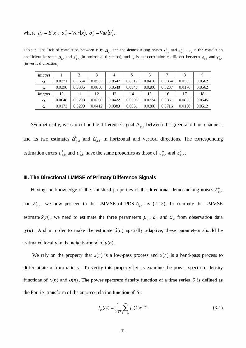
Table 2. The lack of correlation between PDS rg ,∆ and the demosaicking noises h

rg ,ε and vrg ,ε . hc is the correlation

coefficient between rg ,∆ and hrg ,ε (in horizontal direction), and vc is the correlation coefficient between rg ,∆ and v

rg ,ε (in vertical direction).

Images 1 2 3 4 5 6 7 8 9 ch 0.0271 0.0654 0.0502 0.0647 0.0517 0.0410 0.0364 0.0355 0.0562 cv 0.0390 0.0305 0.0836 0.0648 0.0340 0.0200 0.0207 0.0176 0.0562

Images 10 11 12 13 14 15 16 17 18 ch 0.0648 0.0298 0.0390 0.0422 0.0506 0.0274 0.0861 0.0855 0.0645 cv 0.0173 0.0299 0.0412 0.0389 0.0531 0.0200 0.0716 0.0130 0.0512

Symmetrically, we can define the difference signal bg ,∆ between the green and blue channels,

and its two estimates hbg ,∆ and v

bg ,∆ in horizontal and vertical directions. The corresponding

estimation errors hbg ,ε and v

bg ,ε have the same properties as those of hrg ,ε and v

rg ,ε .

III. The Directional LMMSE of Primary Difference Signals

Having the knowledge of the statistical properties of the directional demosaicking noises hrg ,ε

and vrg ,ε , we now proceed to the LMMSE of PDS rg ,∆ by (2-12). To compute the LMMSE

estimate )(ˆ nx , we need to estimate the three parameters xµ , xσ and υσ from observation data

)(ny . And in order to make the estimate )(ˆ nx spatially adaptive, these parameters should be

estimated locally in the neighborhood of )(ny .

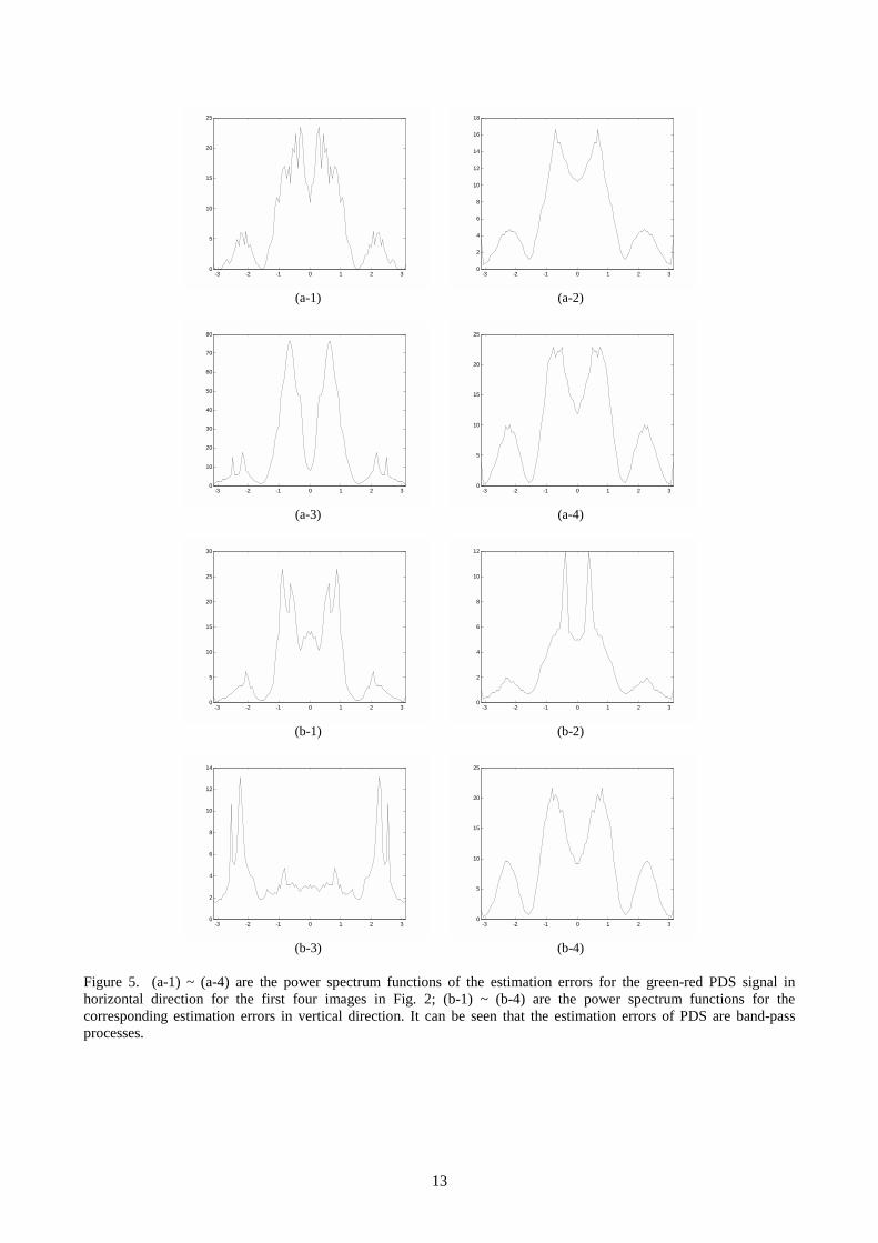
We rely on the property that )(nx is a low-pass process and )(nυ is a band-pass process to

differentiate x from υ in y . To verify this property let us examine the power spectrum density

functions of )(nx and )(nυ . The power spectrum density function of a time series S is defined as

the Fourier transform of the auto-correlation function of S :

∑∞

−∞=

−=k

ikrp ekff ω

πω )(

21)( (3-1)

12

where the sequence )(kfr is the auto-correlation function of S :

)]()([)( knSnSEkfr −⋅= (3-2)

Since )()( kfkf rr −= , (3-1) can be written as

+= ∑∞

=1

)cos()(2)0(21)(

krrp kkfff ω

πω (3-3)

The power spectrum density functions of x and υ are plotted in Fig. 4 and Fig. 5 for some

typical natural images. In Fig. 4 the power spectrum of x for the first four images in Fig. 2 are

plotted, and in Fig. 5 the corresponding power spectrum of υ are illustrated. Obviously, the power

of x concentrates in low frequency band, whereas the power of υ spreads in relatively high

frequency bands.

-3 -2 -1 0 1 2 30

1000

2000

3000

4000

5000

6000

-3 -2 -1 0 1 2 3

0

1

2

3

4

5

6x 104

(a) (b)

-3 -2 -1 0 1 2 30

0.5

1

1.5

2

2.5

3

3.5

4x 104

-3 -2 -1 0 1 2 3

0

1000

2000

3000

4000

5000

6000

7000

8000

9000

10000

(c) (d)

Figure 4. (a) ~ (d) are the power spectrum functions of the green-red difference signals in horizontal direction for the first four images in Fig. 2. The power spectrum functions in vertical direction are similar. It is clear that PDS is a low frequency dominated process.

13

-3 -2 -1 0 1 2 30

5

10

15

20

25

-3 -2 -1 0 1 2 3

0

2

4

6

8

10

12

14

16

18

(a-1) (a-2)

-3 -2 -1 0 1 2 30

10

20

30

40

50

60

70

80

-3 -2 -1 0 1 2 3

0

5

10

15

20

25

(a-3) (a-4)

-3 -2 -1 0 1 2 30

5

10

15

20

25

30

-3 -2 -1 0 1 2 3

0

2

4

6

8

10

12

(b-1) (b-2)

-3 -2 -1 0 1 2 30

2

4

6

8

10

12

14

-3 -2 -1 0 1 2 3

0

5

10

15

20

25

(b-3) (b-4)

Figure 5. (a-1) ~ (a-4) are the power spectrum functions of the estimation errors for the green-red PDS signal in horizontal direction for the first four images in Fig. 2; (b-1) ~ (b-4) are the power spectrum functions for the corresponding estimation errors in vertical direction. It can be seen that the estimation errors of PDS are band-pass processes.

14

Since x and υ have distinct power spectrum, passing y through a low-pass filter can remove

the noises effectively. Denote by { })(kh the response sequence of a low-pass filter, we have

( ) ∑∞

−∞=⋅−=∗=

ks ihinynhyny )()()()( (3-4)

where “*” is the convolution operator. In this paper, we set { })(kh to be the Gaussian smooth filter,

whose coefficients are

2

2

2

21)( σ

σπ

k

ekh−

= (3-5)

where parameter σ controls the shape of the filter response.

Assuming that the random process )(nx is ergodic and stationary, its mean value )(nxµ can be

estimated by the neighboring data of )(ny . The low-pass filter output )(nys is a weighted average

of )(ny and its neighbors, and it is much closer to )(nx than )(ny . Denote by

[ ])()()( LnynyLnyY ssss

n +−= mm (3-6)

the 12 +L dimensional vector centered at )(nys , we estimate )(nxµ as

∑+

=+=

12

1)(

121)(

L

k

snx kY

Lnµ (3-7)

and then we estimate )(2 nxσ , the variance of )(nx , by

∑+

=−

+=

12

1

22 ))()((12

1)(L

kx

snx nkY

Ln µσ (3-8)

Denote by

[ ])()()( LnynyLnyYn +−= mm (3-9)

the 12 +L dimensional vector centered at )(ny . Since )(nys is an approximation of )(nx it follows

that )()( nyny s− is an approximation of )(nυ , thus we can estimate )(2 nυσ , the variance of )(nυ ,

by

15

∑+

=−

+=

12

1

22 ))()((12

1)(L

kn

sn kYkY

Lnυσ (3-10)

For each sample )(nx to be estimated, the corresponding parameters )(nxµ , )(2 nxσ and )(2 nυσ

are computed and substituted into (2-12) to yield )(ˆ nx , the nearly LMMSE estimate of )(nx . Let

)(~ nx be the estimation error of )(nx : )(ˆ)()(~ nxnxnx −= , the variance of )(~ nx is

))()(()()()](~[)( 22

2222

~nn

nnnxEnx

xxx

υσσσσσ

+−== (3-11)

IV. Optimal Fusion of the Directional LMMSE Estimates

Using the scheme developed in the previous section, two LMMSE estimates of a PDS signal

)(nx can be obtained, respectively in the horizontal and vertical directions, which are denoted by

)(ˆ nxh and )(ˆ nxv . Let )(~ nxh and )(~ nxv be the corresponding estimation errors, then

−=−=

)(~)()(ˆ)(~)()(ˆ

nxnxnxnxnxnx

vv

hh (4-1)

The variances of estimation errors )(~ nxh and )(~ nxv are denoted by )(2~ n

hxσ and )(2~ n

vxσ .

Either )(ˆ nxh or )(ˆ nxv exploits the correlation of )(nx with its neighbors in a particular

direction. A more accurate estimate of )(nx can be obtained by fusing the two directional LMMSE

estimates. We employ the weighted average strategy and let the fused estimate be

)(ˆ)()(ˆ)()(ˆ nxnwnxnwnx vvhhw ⋅+⋅= (4-2)

where 1)()( =+ nwnw vh . The weights )(nwh and )(nwv are determined to minimize the mean

square-error of )(ˆ nxw :

]))(ˆ)([()](~[)( 222~ nxnxEnxEn wwxw

−==σ (4-3)

or

)](~)(~[)()(2)()()()()( 2~

22~

22~ nxnxEnwnwnnwnnwn vhvhxvxhx vhw

⋅⋅⋅⋅+⋅+⋅= σσσ (4-4)

16

Generally, the correlation between variables hx~ and vx~ is weak for a natural image, especially in

the areas of edges and fine texture structures where the human visual system is sensitive to spatial

resolution. In fact, if hx~ and vx~ are highly correlated, i.e., the two estimates hx and vx are close to

each other, then wx varies little in hw and vw anyways.

Assuming that hx~ and vx~ are approximately uncorrelated, the magnitude of the last term in the

right side of (4-4) becomes negligible, or approximately

)()(2)())()(()(

)()()()()(2~

2~

2~

2~

2

2~

22~

22~

nnwnnnnw

nnwnnwn

vvvh

vhw

xhxxxh

xvxhx

σσσσ

σσσ

⋅⋅−++⋅=

⋅+⋅≈ (4-5)

To minimize )(2~ n

wxσ , we let the partial differential of )(2~ n

wxσ with respect to )(nwh be zero, namely

0)(2))()(()(2)()( 2

~2~

2~

2~

=⋅−+⋅⋅=∂∂

nnnnwnwn

vvh

wxxxh

h

x σσσσ

(4-6)

Finally we have

)()()(

)( 2~

2~

2~

nnn

nwvh

v

xx

xh σσ

σ+

= , )()(

)()( 2

~2~

2~

nnn

nwvh

h

xx

xv σσ

σ+

= (4-7)

Substituting (4-7) into (4-2) yields )(ˆ nxw , the optimally weighted estimate of )(ˆ nxh and )(ˆ nxv . The

MSE of the optimal estimate )(ˆ nxw is

)()()()(

)( 2~

2~

2~

2~2

~nn

nnn

vh

vh

wxx

xxx σσ

σσσ

+= (4-8)

Obviously )(2~ n

wxσ is less than either of )(2~ n

hxσ and )(2~ n

vxσ .

Using the method described in Sections III and IV, we compute, for each red pixel position nR

and each blue pixel position nB , the directional weighted estimates of the green-red PDS signal

)(, nrg∆ and the green-blue PDS signal )(, nbg∆ . Then we can recover the green channel of the Bayer

CFA image by estimating the missing green samples as

17

)(RG , nrgnn ∆+= or )(BG , nbgnn ∆+= (4-9)

Compared with the red and blue channels of a Bayer CFA image, the green channel preserves much

more detail of the image and hence is more important for the human visual system. Furthermore, the

interpolation quality of red and blue channels, which is the subject of the next section, also depends

on the estimation accuracy of the green channel.

V. The Demosaicking of the Chrominance Channels

In the previous two sections we showed how to remove the demosaicking noise in the green

channel by directional LMMSE filtering of PDS and optimal fusing of the resulting directional

LMMSE estimates. Once the robust green estimates are obtained for all pixels, they can guide, in

conjunction with the PDS estimates, the demosaicking of the red and blue channels. This is

accomplished in the following two steps.

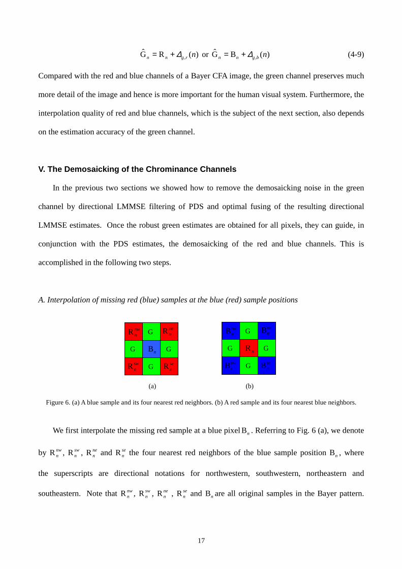
A. Interpolation of missing red (blue) samples at the blue (red) sample positions

(a) (b)

Figure 6. (a) A blue sample and its four nearest red neighbors. (b) A red sample and its four nearest blue neighbors.

We first interpolate the missing red sample at a blue pixel nB . Referring to Fig. 6 (a), we denote

by nwnR , sw

nR , nenR and se

nR the four nearest red neighbors of the blue sample position nB , where

the superscripts are directional notations for northwestern, southwestern, northeastern and

southeastern. Note that nwnR , sw

nR , nenR , se

nR and nB are all original samples in the Bayer pattern.

G

G

G

G

nwnR ne

nR

senRsw

nR

nB G

G

G

G

nwnB ne

nB

senBsw

nB

nR

18

The estimated green samples at these positions are denoted by nG , nwnG , sw

nG , nenG and se

nG

respectively. The available four green-red difference values are represented as nwgrn,∆ , sw

grn,∆ , negrn,∆

and segrn,∆ . The estimate nR of the missing red sample is to be computed.

We interpolate the green-red PDS signal at the blue sample position nB as the average of the

four available green-red differences, namely

4,,,,

,

swgrn

negrn

segrn

nwgrn

grn

∆∆∆∆∆

+++= (5-1)

Then the missing red sample is estimated as

grnnn ,GR ∆−= (5-2)

Similarly, the missing blue samples at the red sample positions nR (referring to Fig. 6 (b)) can

be interpolated. The four green-blue difference values in the northwestern, southwestern,

northeastern and southeastern of nR are available, and they are averaged to interpolate the green-

blue PDS signal gbn,∆ at position nR . The missing blue sample is then estimated as

gbnnn ,GB ∆−= .

B. Interpolation of missing red/blue samples at the green sample positions

(a) (b) (c) (d)

Figure 7. (a) ~ (b) A green sample and its two original and two estimated red neighbors. (c) ~ (d) A green sample and its two original and two estimated blue neighbors.

After the missing red/blue samples at the blue/red positions have been filled, we arrive at the

G G

wnR e

nR

G G

nG

nnR

snR G G

wnR e

nR

G G

nG

nnR

snR G G

wnB e

nB

G G

nG

nnB

snB G G

wnB e

nB

G G

nG

nnB

snB

19

four cases depicted by Fig. 7. As before, the samples are estimated ones if marked by “^”, and

original ones otherwise. Due to the symmetry between red and blue samples in these four cases, we

only need to discuss case (a). Given the green estimates nnG , s

nG , enG and w

nG at the positions nnR ,

snR , e

nR , and wnR , we have the corresponding four green-red difference values, denoted by n

grn,∆ ,

sgrn,∆ , e

grn,∆ and wgrn,∆ . As in the previous step, we compute the bilinear average of the green-red

differences

( )4

,,,,,

wgrn

egrn

sgrn

ngrn

grn

∆∆∆∆∆

+++= (5-3)

Then the missing red sample at green sample position nG is estimated to be grnnn ,GR ∆−= .

Similarly, the missing blue sample at a green position nG is estimated as gbnnn ,GB ∆−= .

By now we have filled in all the missing red/blue samples. The full color image is

reconstructed. The presented demosaicking scheme first exploits the correlation between the green

and red/blue channels to obtain good estimates of the missing green samples, and then estimates the

missing red and blue samples by a simple and fast bilinear average operation on the green-red and

green-blue PDS signals.

VI. Experimental Results

We implemented the proposed LMMSE color demosaicking algorithm, and tested it on a large

number of natural color images. In this section we present our experimental results for the eighteen

images of Fig. 2, and compare them with the methods of Hamilton et al. [2], Chang et al. [7] and

Gunturk et al. [9], which are among the most popular schemes. The results reported in the recent

paper of [9] were better than the previously published algorithms, especially for the red and blue

channels. In the implementation of our scheme, the standard deviation of the Gaussian smooth filter,

σ (referring to (3-5)), was set around 2, and the parameter L (referring to (3-6) and (3-9)) was set

20

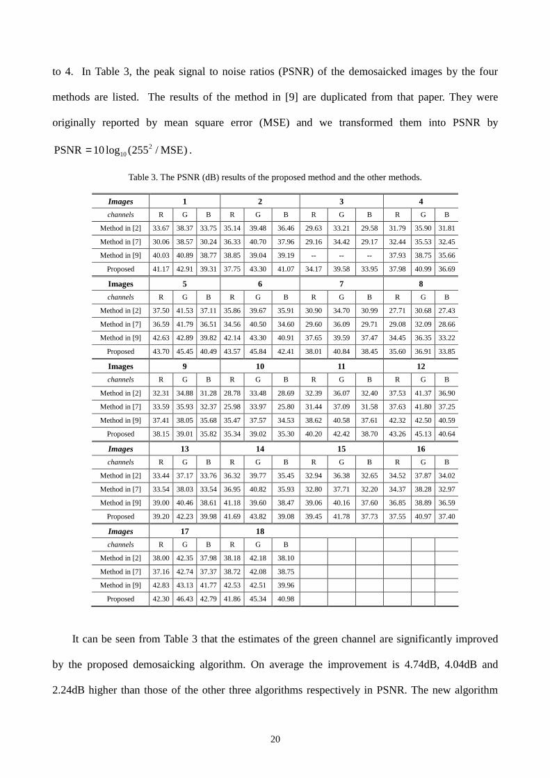
to 4. In Table 3, the peak signal to noise ratios (PSNR) of the demosaicked images by the four

methods are listed. The results of the method in [9] are duplicated from that paper. They were

originally reported by mean square error (MSE) and we transformed them into PSNR by

)MSE/255(log10PSNR 210= .

Table 3. The PSNR (dB) results of the proposed method and the other methods.

Images 1 2 3 4 channels R G B R G B R G B R G B

Method in [2] 33.67 38.37 33.75 35.14 39.48 36.46 29.63 33.21 29.58 31.79 35.90 31.81

Method in [7] 30.06 38.57 30.24 36.33 40.70 37.96 29.16 34.42 29.17 32.44 35.53 32.45

Method in [9] 40.03 40.89 38.77 38.85 39.04 39.19 -- -- -- 37.93 38.75 35.66

Proposed 41.17 42.91 39.31 37.75 43.30 41.07 34.17 39.58 33.95 37.98 40.99 36.69

Images 5 6 7 8 channels R G B R G B R G B R G B

Method in [2] 37.50 41.53 37.11 35.86 39.67 35.91 30.90 34.70 30.99 27.71 30.68 27.43

Method in [7] 36.59 41.79 36.51 34.56 40.50 34.60 29.60 36.09 29.71 29.08 32.09 28.66

Method in [9] 42.63 42.89 39.82 42.14 43.30 40.91 37.65 39.59 37.47 34.45 36.35 33.22

Proposed 43.70 45.45 40.49 43.57 45.84 42.41 38.01 40.84 38.45 35.60 36.91 33.85

Images 9 10 11 12 channels R G B R G B R G B R G B

Method in [2] 32.31 34.88 31.28 28.78 33.48 28.69 32.39 36.07 32.40 37.53 41.37 36.90

Method in [7] 33.59 35.93 32.37 25.98 33.97 25.80 31.44 37.09 31.58 37.63 41.80 37.25

Method in [9] 37.41 38.05 35.68 35.47 37.57 34.53 38.62 40.58 37.61 42.32 42.50 40.59

Proposed 38.15 39.01 35.82 35.34 39.02 35.30 40.20 42.42 38.70 43.26 45.13 40.64

Images 13 14 15 16 channels R G B R G B R G B R G B

Method in [2] 33.44 37.17 33.76 36.32 39.77 35.45 32.94 36.38 32.65 34.52 37.87 34.02

Method in [7] 33.54 38.03 33.54 36.95 40.82 35.93 32.80 37.71 32.20 34.37 38.28 32.97

Method in [9] 39.00 40.46 38.61 41.18 39.60 38.47 39.06 40.16 37.60 36.85 38.89 36.59

Proposed 39.20 42.23 39.98 41.69 43.82 39.08 39.45 41.78 37.73 37.55 40.97 37.40

Images 17 18 channels R G B R G B

Method in [2] 38.00 42.35 37.98 38.18 42.18 38.10

Method in [7] 37.16 42.74 37.37 38.72 42.08 38.75

Method in [9] 42.83 43.13 41.77 42.53 42.51 39.96

Proposed 42.30 46.43 42.79 41.86 45.34 40.98

It can be seen from Table 3 that the estimates of the green channel are significantly improved

by the proposed demosaicking algorithm. On average the improvement is 4.74dB, 4.04dB and

2.24dB higher than those of the other three algorithms respectively in PSNR. The new algorithm

21

also outperforms the other algorithms in red and blue channels as well. The margins of

improvement in PSNR are 5.87dB and 6.23dB over the algorithm of [2] and the algorithm of [7] for

the red channel, and respectively 5.06dB and 5.46dB for the blue channel. Compared with the

algorithm of [9], the new algorithm achieves 0.46dB higher PSNR in the red channel and 0.84dB

higher PSNR in the blue channel. One should keep in mind that the demosaicking results of [9] in

the red and blue channels were obtained by costly eight iterations of wavelet-based filtering

operations, while our results were obtained by simple bilinear interpolation of the primary

difference signals. The computation and implementation complexities are considerably lower than

[9].

In Fig. 8 ~ Fig. 13, some samples of the original and the demosaicked images by different

methods ([2], [7] and the proposed) are shown for the purpose of subjective quality evaluation. For

the visual results of [9] the reader can refer to the original paper. The proposed LMMSE-based

demosaicking algorithm appears to produce visually more pleasant color images with color artifacts

greatly suppressed.

VII. Conclusion

This paper presented a new color demosaicking technique of LMMSE directional filtering of the

green-red and green-blue PDS signals. The missing green samples are estimated from the filtered

PDS in both horizontal and vertical directions, and the two estimates are optimally fused. The

resulting green channel is then used to guide the estimation of the missing red and blue samples.

The experiments showed that the proposed color demosaicking algorithm significantly

outperformed the current state of the art demosaicing methods both in PSNR measure and visual

quality. Furthermore, the proposed algorithm is non-iterative, fast, and easy to implement.

References

22

[1] J. E. Adams, “Intersections between color plane interpolation and other image processing

functions in electronic photography,” Proceedings of SPIE, vol. 2416, pp. 144-151, 1995.

[2] J. E. Adams and J. F. Hamilton Jr., “Adaptive color plane interpolation in single color

electronic camera,” U. S. Patent, 5 506 619, 1996.

[3] J. E. Adams, “Design of practical color filter array interpolation algorithms for digital

cameras,” Proceedings of SPIE, vol. 3028, pp. 117-125, 1997.

[4] D. Alleysson, S. Süsstrunk and J. Hérault, “Color demosaicking by estimating luminance and

opponent chromatic signals in the Fourier domain,” Proc. 10th Color Imaging Conference, pp.

331-336, 2002.

[5] B. E. Bayer and Eastman Kodak Company, “Color Imaging Array,” US patent 3 971 065, 1975.

[6] D. R. Cok and Eastman Kodak Company, “Signal Processing method and apparatus for

producing interpolated chrominance values in a sampled color image signal,” US patent 4 642

678, 1987.

[7] E. Chang, S. Cheung and D. Y. Pan, “Color filter array recovery using a threshold-based

variable number of gradients,” Proceedings of SPIE, vol. 3650, pp. 36-43, 1999.

[8] W. T. Freeman, “Method and apparatus for reconstructing missing color samples,” U. S.

Patents, 4 663 655.

[9] B. K. Gunturk, Y. Altunbasak and R. M. Mersereau, “Color plane interpolation using

alternating projections,” IEEE Trans. Image Processing, vol. 11, pp. 997-1013, 2002.

[10] H. S. Hou et al, “Cubic splines for image interpolation and digital filtering,” IEEE Trans.

Acoustic, Speech and Signal Processing, vol. ASSP-26, pp. 508-517, 1987.

[11] J. F. Hamilton Jr. and J. E. Adams, “Adaptive color plane interpolation in single sensor color

electronic camera,” U. S. Patent, 5 629 734, 1997.

[12] R. H. Hibbard, “Apparatus and method for adaptively interpolation a full color image utilizing

luminance gradients,” U. S. Patent 5 382 976, 1995.

23

[13] R. Kimmel, “Demosaicing: Image reconstruction from CCD samples,” IEEE Trans. Image

Processing, vol. 8, pp. 1221-1228, 1999.

[14] E. W. Karmen and J. K. Su, Introduction to optimal estimation, Springer-Verlag London

Limited, 1999.

[15] P. Longère, Xuemei Zhang, P. B. Delahunt and Davaid H. Brainard, “Perceptual assessment of

demosaicing algorithm performance,” Proc. of IEEE, vol. 90, pp. 123-132, 2002.

[16] C. A. Laroche and M. A. Prescott, “Apparatus and method for adaptively interpolating a full

color image utilizing chrominance gradients,” U. S. Patent 5 373 322, 1994.

[17] William K. Pratt, Digital Image Processing, John Wiley & Sons, 2nd edition, April 1991.

[18] R. Ramanath and W. E. Snyder, “Adaptive demosaicking,” Journal of Electronic Imaging, vol.

12, No. 4, pp. 633-642, 2003.

[19] H. J. Trussel and R. E. Hartwing, “Mathematics for demosaicking,” IEEE Trans. Image

Processing, vol. 11, pp. 485-492, 2002.

[20] J. A. Weldy, “Optimized design for a single-sensor color electronic camera system,”

Proceedings of SPIE, vol. 1071, pp. 300-307, 1988.

[21] X. Wu, W. K. Choi and Paul Bao, “Color restoration from digital camera data by pattern

matching,” Proceedings of SPIE, vol. 3018, pp. 12-17, 1997.

24

(a) (b)

(c) (d)

Figure 8. Demosaicked results of image 1 in Fig. 2: (a) Original; (b) Method in [2]; (c) Method in [7]; (d) The proposed method.

(a) (b)

(c) (d)

Figure 9. Demosaicked results of image 2 in Fig. 2: (a) Original; (b) Method in [2]; (c) Method in [7]; (d) The proposed method.

25

(a) (b)

(c) (d)

Figure 10. Demosaicked results of image 3 in Fig. 2: (a) Original; (b) Method in [2]; (c) Method in [7]; (d) The proposed method.

(a) (b)

(c) (d)

Figure 11. Demosaicked results of image 4 in Fig. 2: (a) Original; (b) Method in [2]; (c) Method in [7]; (d) The proposed method.

26

(a) (b)

(c) (d)

Figure 12. Demosaicked results of image 11 in Fig. 2: (a) Original; (b) Method in [2]; (c) Method in [7]; (d) The proposed method.

(a) (b)

(c) (d)

Figure 13. Demosaicked results of image 10 in Fig. 2: (a) Original; (b) Method in [2]; (c) Method in [7]; (d) The proposed method.