communications technology power and energy · chapter 10 of electric power system basics for the...
TRANSCRIPT

Wiley-IEEE Press Sampler
Communications Technology Power and Energy

Contents
5G STANDARD DEVELOPMENT: TECHNOLOGY AND ROADMAP By Juho Lee and Yongjun Kwak Chapter 23 of Signal Processing for 5G: Algorithms and Implementations
WHY IS PM IMPORTANT, ESPECIALLY IN TELECOMMUNICATIONS By Celia Desmond Chapter 2 of The ComSoc Guide to Managing Telecommunication Projects
PERSONAL PROTECTION (SECURITY) By Steven W. BlumeChapter 10 of Electric Power System Basics for the Nonelectrical Professional, Second Edition
PREDICTIVE CONTROL OF A THREE-PHASE INVERTERBy Jose Rodriguez and Patricio CortesChapter 4 of Predictive Control of Power Converters and Electrical Drives
Interested in learning more about the custom digital solutions Wiley-IEEE Press
can offer your business?Contact Donna Marcum at [email protected] or 317-572-3508.
�
� �
�
235G Standard Development:Technology and Roadmap
Juho Lee and Yongjun Kwak
23.1 Introduction 561
23.2 Standards Roadmap from 4G to 5G 562
23.3 Preparation of 5G Cellular Communication Standards 570
23.4 Concluding Remarks 575
References 575
23.1 Introduction
The wireless cellular network has been one of the most successful communications technolo-gies of the last three decades. The advent of smartphones and tablets over the past several yearshas resulted in an explosive growth of data traffic. With the proliferation of more smart termi-nals communicating with servers and each other via broadband wireless networks, numerousnew applications have also emerged to take advantage of wireless connectivity.
As 4G LTE-Advanced [1, 2] networks mature and become a global commercial success, theresearch community is now increasingly looking at future 5G technologies, both in standard-ization bodies such as 3GPP and in research projects such as the EU’s FP7 METIS [3]. ITU-Rhas recently finalized their work on the vision for 5G systems, which includes support for anexplosive growth of data traffic, support for a massive number of machine-type communica-tion (MTC) devices, and support for ultra-reliable and low-latency communications [4]. Whiletoday’s commercial 4G LTE-Advanced networks are mostly deployed in legacy cellular bandsfrom 600 MHz to 3.5 GHz, recent technological advances will allow 5G to utilize any spectrumopportunities below 100 GHz, including existing cellular bands, new bands below 6 GHz, and
Signal Processing for 5G: Algorithms and Implementations, First Edition. Edited by Fa-Long Luo and Charlie Zhang.© 2016 John Wiley & Sons, Ltd. Published 2016 by John Wiley & Sons, Ltd.
�
� �
�
562 Signal Processing for 5G
new bands above 6 GHz including the so-called mmWave bands. There are coordinated effortsacross the world to identify these new spectrum opportunities, with decisions expected for newfrequency bands below 6 GHz at the World Radio-communication Conference (WRC)-2015,and for new frequency bands above 6 GHz at WRC-2019, respectively.
From the 5G technology roadmap perspective, we expect a dual-track approach to take placeover the next few years in 3GPP. The first track is commonly known as the evolution track,where we expect that the evolution of LTE-Advanced will continue in Rel-13/14 and beyond ina backward-compatible manner with the goal of improving system performance in the bandsbelow 6 GHz. It is also our expectation that at least a part of the 5G requirements could be metby the continued evolution of LTE-Advanced. For example, latency reduction with grant-lessuplink access and shortened transmission time interval (TTI) could reduce over-the-air latencyto less than 1 ms. The second track is commonly known as new radio access technology (RAT)track, which is not limited by backward-compatibility requirements and can integrate break-through technologies to achieve the best possible performance. The new RAT system shouldmeet all 5G requirements as it would eventually need to replace the previous generation sys-tems in the future. The new RAT track is also expected to have a scalable design that canseamlessly support communications in both above and below 6 GHz bands.
The rest of this chapter is organized into the following three sections, focusing on the tech-nologies for the air interface of radio access networks. Section 23.2 is devoted to the standardsroadmap from 4G to 5G. In Section 23.3, we will provide an overview of major enabling tech-nologies and a more detailed roadmap of the 5G standard development and its deployment.Section 23.4 is the final section, which presents the summary of this chapter.
23.2 Standards Roadmap from 4G to 5G
Since the publication of the Rel-99 standards supporting wideband code division multipleaccess (WCDMA) – a representative 3G technology – 3GPP has been playing an importantrole in evolving cellular communication standards to 4G, namely LTE and LTE-Advanced.3GPP is a partnership project between regional standardization bodies, or organizational part-ners (OPs). 3GPP was established in 1998 and has seven OPs as of 2015: ARIB and TTC fromJapan, ATIS from USA, CCSA from China, ETSI from Europe, TSDSI from India, and TTAfrom Korea. After the success of 3G technologies, 3GPP introduced LTE as Rel-8 in 2009, andLTE-Advanced as Rel-10 in 2011, the latter declared by ITU-R “IMT-Advanced technology”and often called 4G. There has been continuing further evolution toward 5G. The 3GPP orga-nization and its overall roadmap from LTE in Rel-8 to LTE-Advanced in Rel-13 are shown inFigures 23.1 and 23.2, respectively. The project coordination group coordinates the projectsperformed in 3GPP. Each technical specification group (TSG) decides whether specificationsfor a technology will be developed, typically taking into account the outcome of the relatedfeasibility study in its working groups (WGs). WGs develop technical specifications, whichare then formally approved by their TSG.
LTE in Rel-8 was the first standard in 3GPP that utilized frequency division multiplexing:orthogonal frequency division multiplexing (OFDM) in the downlink and single carrierfrequency division multiple access (SC-FDMA) in the uplink as illustrated in Figure 23.3.SC-FDMA is a variant of OFDM, where discrete Fourier transform (DFT) processing isapplied to the input signal before inverse DFT (IDFT) so that the output of IDFT mimics asingle carrier signal. The peak-to-average power ratio of SC-FDMA is smaller than that of

�
� �
�
5G Standard Development: Technology and Roadmap 563
Project Coordination Group
(PCG)
TSG CTCore Network
& Terminals
CT WG1 MM/CC/SM (lu)
CT WG3 Interworking with
External Networks
CT WG4 MAP/GTP/BCH/SS
CT WG6Smart Card
Application Aspects
TSG RANRadio Access Network
RAN WG1Radio Layer 1
RAN WG2Radio Layer 2 &
Radio Layer 3
RAN WG3lu, lub, lur, S1, X2,
and UTRAN/E-UTRAN
RAN WG4Radio Performance
& Protocol Aspects
RAN WG5Mobile Terminal
Conformance Testing
TSG SAService &
System Aspects
SA WG1Services
SA WG2Architecture
SA WG3Security
SA WG4Codec
SA WG5Telecom Management
SA WG6Mission-Critical
Applications
RAN WG6GERAN Aspects
Figure 23.1 3GPP organization
LTE-AdvancedLTE
Rel-8
Mar 2009 Mar 2010 June 2011 Mar 2013 Mar 2015 Mar 2016
Rel-9 Rel-10 Rel-11 Rel-12 Rel-13
Figure 23.2 Overall roadmap from LTE in Rel-8 to LTE-Advanced in Rel-13
an OFDM signal and hence SC-FDMA helps increase the uplink coverage. The maximumbandwidth is 20 MHz, providing a 300 Mbps peak rate on the downlink with 4× 4 MIMOand a 75 Mbps peak rate on the uplink. It is worth noting that the OFDM waveform on thedownlink does not require a complicated equalization at the user equipment1 (UE) receiverand hence helps reduce UE receiver complexity. This property motivated the specificationof 4 × 4 MIMO on downlink from the very first release of LTE. LTE Rel-9 included a few
1 3GPP terminology for a mobile device.

�
� �
�
564 Signal Processing for 5G
IDFT
DFT
S0 S1 S2 …… S10 S11
Freq.
(a) (b)
Figure 23.3 Signal generation for (a) OFDM on downlink and (b) SC-FDMA on uplink
Contiguous Intra-band Carrier Aggregation of five CCs (20 MHz CC × 5)
Non-contiguous Intra-band Carrier Aggregation of 3 CCs (20 MHz CC × 3)
Inter-band Carrier Aggregation of 2 CCs (20 MHz CC × 2)
f
f
fBand yBand x
Figure 23.4 A few examples of carrier aggregation with up to five component carriers (CCs)
additional features, for example emergency call, that was required to support voice callsover LTE.
LTE-Advanced standard in Rel-10 was developed to meet not only IMT-Advanced require-ments but also commercial requests for accommodating increased data traffic. As a naturalapproach for increasing the peak rate, aggregation of up to five component carriers was spec-ified, resulting in the use of 100 MHz at maximum. A few examples of carrier aggregationare shown in Figure 23.4. It should be noted that carrier aggregation has been one of the mostsuccessful features of LTE-Advanced because it enables mobile network operators to providehigher peak rates and to improve the operational efficiency of radio access networks by uti-lizing scattered frequency resources. In addition, MIMO was further enhanced through theintroduction of 8 × 8 MIMO and 4 × 4 MIMO on the downlink and uplink, respectively.A combination of carrier aggregation and the larger order of MIMO provided 3 Gbps and1.5 Gbps peak rates on the downlink and uplink, respectively.

�
� �
�
5G Standard Development: Technology and Roadmap 565
Support of MIMO with eight transmit antennas at the enhanced Node B2 (eNB) necessitatedintroduction of a UE-specific demodulation reference signal (DM-RS) together with a channelstatus information reference signal (CSI-RS). This is because too much overhead results fromincreasing the number of common reference signal (CRS) ports, which are transmitted in acontinuous manner (in every subframe). The DM-RS is transmitted, and introduces overhead,only for the UEs to which downlink transmissions are scheduled, and the CSI-RS overhead canbe minimized by increasing its transmission period as shown in Figure 23.5, where RE, RB,and PRB denote resource element, resource block, and physical resource block, respectively.
While the carrier aggregation and MIMO are mainly aimed at increasing the peak rate, sup-port of heterogeneous networks consisting of macro and pico cells on the same frequency layerby relying on time-domain interference coordination is a remarkable step that significantlyimproves the spectrum-utilization efficiency.
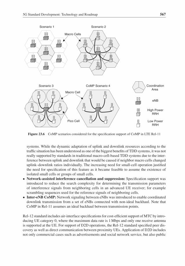
Following the improvements in peak data rates and system capacity provided by MIMOin LTE and LTE-Advanced, it was also shown to be possible to provide further performanceimprovement by having coordinated transmission and reception between multiple points [5],where a point can be treated as a set of geographically co-located transmit antennas, with theexception that sectors of the same site are considered different points. The Rel-11 standardintroduced specification support for coordinated transmission in the downlink and coordi-nated reception in the uplink, which is commonly denoted coordinated multipoint (CoMP).The assumed deployment scenarios for CoMP illustrated in Figure 23.6 include homogeneousconfigurations, where the points are different cells, as well as heterogeneous configurations,where a set of low power points – for example remote radio heads (RRHs) or pico cells – arelocated in the geographical area served by a macro cell. For coordinated transmission in thedownlink, the signals transmitted from multiple transmission points are coordinated to improvethe received strength of the desired signal at the UE or to reduce the co-channel interference.The major purpose of coordinated reception in the uplink is to help ensure that the uplink sig-nal from the UE is reliably received by the network while limiting uplink interference, takinginto account the existence of multiple reception points.
While Rel-12 continued the evolution towards improving the peak rate by aggregating theavailable frequency resource and improving spectral efficiency, it also started specificationof features that were required for support of new services such as machine-type communica-tions and device-to-device communications (D2D) that had not been a major focus of previousreleases. The features of the first category include the following:
• Small cell enhancement: Dual connectivity was introduced to enable a UE to connectto both the macro cell layer, which provides mobility support on lower frequencies, say700 MHz, and the small cell layer, which provides a fat data pipe on higher frequencies, say3.5 GHz.
• Time division duplex (TDD)-frequency division duplex (FDD) joint operations: Jointoperations of both TDD and FDD carriers is important and useful for mobile network oper-ators owning both TDD and FDD carriers. In order to enable this, the carrier aggregationbetween TDD and FDD carriers was specified in Rel-12.
• Enhanced interference management and traffic adaptation for TDD: This feature intro-duced specified support of dynamic adjustment of uplink and downlink resources in TDD
2 3GPP terminology for a base station.

�
� �
�
566 Signal Processing for 5G
PR
B 0
P
RB
1
PR
B 2
P
RB
3
PR
B 5
PR
B 4
Subframe 0 Subframe 1 Subframe 2 Subframe 3 Subframe 4 Subframe 5 Subframe 6 Subframe 7 Subframe 8 Subframe 9
CSI-RS subframes
Scheduled RBs
: CRS REs : CSI-RS REs : DM-RS REs
Figure 23.5 Downlink MIMO support in LTE-Advanced with DM-RS and CSI-RS
�
� �
�
5G Standard Development: Technology and Roadmap 567
eNB
Coordination
Area
High Power
RRH
Low Power
RRH
Macro Cells
Scenario 1 Scenario 2
Pico Cell
Scenario 3 CoMP Scenario 4
Macro Cell
Figure 23.6 CoMP scenarios considered for the specification support of CoMP in LTE Rel-11
systems. While the dynamic adaptation of uplink and downlink resources according to thetraffic situation has been understood as one of the biggest benefits of TDD systems, it was notreally supported by standards in traditional macro-cell-based TDD systems due to the inter-ference between uplink and downlink that would be caused if neighbor macro cells changeduplink–downlink ratios individually. The increasing need for small-cell operation justifiedthe need for specification of this feature as it became feasible to assume the existence ofisolated small cells or groups of small cells.
• Network-assisted interference cancellation and suppression: Specification support wasintroduced to reduce the search complexity for determining the transmission parametersof interference signals from neighboring cells in an advanced UE receiver; for examplescrambling sequences used for the reference signals of neighboring cells.
• Inter-eNB CoMP: Network signaling between eNBs was introduced to enable coordinateddownlink transmission from a set of eNBs connected with non-ideal backhaul. Note thatCoMP in Rel-11 assumes an ideal backhaul between transmission points.
Rel-12 standard includes air-interface specifications for cost-efficient support of MTC by intro-ducing UE category 0, where the maximum data rate is 1 Mbps and only one receive antennais supported at the UE. For support of D2D operations, the Rel-12 standard specified peer dis-covery as well as direct communication between proximity UEs. Application of D2D includesnot only commercial cases such as advertisements and social network service, but also public

�
� �
�
568 Signal Processing for 5G
safety operations especially for the case when mobile networks have collapsed, for exampledue to earthquakes.
In the continued evolution of LTE-Advanced in Rel-13 and Rel-14, it is important to empha-size continuity and backward compatibility in order to leverage the massive economies of scaleassociated with the current ecosystem that has developed around the LTE/LTE-Advanced stan-dards from Rel-8 to Rel-12. While improving the spectral efficiency has traditionally beenemphasized, the importance of supporting diverse requests from mobile network operatorswas also well recognized in planning the features to be standardized in Rel-13 and upwards.As the result of this consideration, Rel-13 includes the following major features:
• full dimension MIMO (FD-MIMO) for a drastic increase of spectral efficiency via use of alarge number of antennas at the base station,
• licensed assisted access (LAA) for utilizing unlicensed spectrum while guaranteeing coex-istence with existing devices,
• carrier aggregation with up to 32 component carriers,• further cost reductions for MTC devices that can also support extended coverage.
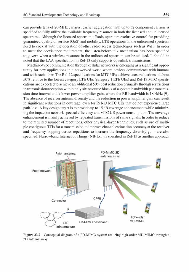
FD-MIMO heavily relies on advancement of signal processing technologies and is one ofthe key candidate technologies for the evolution from 4G to 5G cellular systems. The keyidea behind FD-MIMO is to utilize a large number of antennas placed in a two-dimensional(2D) antenna-array panel for forming narrow beams in both the horizontal and vertical direc-tions. Such beamforming allows an eNB to perform simultaneous transmissions to multipleUEs, realizing high-order multi-user spatial multiplexing. Figure 23.7 depicts an eNB withFD-MIMO implemented using a 2D antenna array panel, where every antenna is an activeelement allowing dynamic and adaptive precoding across all antennas. By utilizing such pre-coding, the eNB can simultaneously direct transmissions in the azimuth and elevation domainsfor multiple UEs. The key feature of FD-MIMO in improving the system performance is itsability to realize high-order multi-user multiplexing.
3GPP has conducted several studies since December 2012 in an effort to provide spec-ification support for FD-MIMO. The first step was a study for developing a new channelmodel for future evaluation of antenna technologies based on 2D antenna-array panels [6].The channel model provides the stochastic characteristics of a three-dimensional (3D) wire-less channel. Based on the new channel model, a follow-up study item on FD-MIMO wasinitiated in September 2014 to evaluate the performance of FD-MIMO and identify key areasin LTE specifications that need to be enhanced in order to support 2D arrays with up to 64antenna ports [7]. In June 2015, 3GPP started a work item to specify FD-MIMO operationsfor LTE-Advanced in Rel-13. FD-MIMO has two important differentiating factors compared toMIMO technologies from previous LTE releases. First, the number of antenna ports at the eNBtransmitter is increased from 8 to 16. As a result, FD-MIMO significantly improves beamform-ing and spatial user multiplexing capabilities. Second, specification support for FD-MIMO istargeted for antennas placed on a 2D planar array. Using the 2D planar placement is also helpfulto reduce the form factor of the antennas for practical applications.
LAA aims to use unlicensed spectrum as a complement for LTE systems operating inlicensed spectrum to meet the sharply increased demand for wireless broadband data [8]. Fortight integration of the unlicensed spectrum as a capacity boost with the licensed spectrum,LAA uses carrier aggregation. Considering the availability of the 5-GHz unlicensed band that
�
� �
�
5G Standard Development: Technology and Roadmap 569
can provide tens of 20-MHz carriers, carrier aggregation with up to 32 component carriers isspecified to fully utilize the available frequency resource in both the licensed and unlicensedspectrums. Although the licensed spectrum affords operators exclusive control for providingguaranteed quality of service (QoS) and mobility, LTE operations in the unlicensed spectrumneed to coexist with the operation of other radio access technologies such as WiFi. In orderto meet the coexistence requirement, the listen-before-talk mechanism has been specifiedto govern when a wireless resource in the unlicensed spectrum can be utilized. It should benoted that the LAA specification in Rel-13 only supports downlink transmissions.
Machine-type communication through cellular networks is emerging as a significant oppor-tunity for new applications in a networked world where devices communicate with humansand with each other. The Rel-12 specifications for MTC UEs achieved cost reductions of about50% relative to the lowest category LTE UEs (category 1 LTE UEs) and Rel-13 MTC specifi-cations are expected to achieve an additional 50% cost reduction primarily through restrictionsin transmission/reception within only six resource blocks of a system bandwidth per transmis-sion time interval and a lower power amplifier gain, where the RB bandwidth is 180 kHz [9].The absence of receiver antenna diversity and the reduction in power amplifier gain can resultin significant reductions in coverage, even for Rel-13 MTC UEs that do not experience largepath-loss. A key design target is to provide up to 15 dB coverage enhancement while minimiz-ing the impact on network spectral efficiency and MTC UE power consumption. The coverageenhancement is mainly achieved by repeated transmissions of same signals. In order to reduceto the required number of repetitions, other physical-layer techniques, such as use of multi-ple contiguous TTIs for a transmission to improve channel estimation accuracy at the receiverand frequency hopping across repetitions to increase the frequency diversity gain, are alsospecified. Narrowband Internet of Things (NB-IoT) is specified in Rel-13 as another approach
Patch antenna
Feed network
Connector
IP
CPRI
High-order
MU-MIMOFD-MIMO baseband
FD-MIMO 2D
antenna array
LTE
infrastructure
Figure 23.7 Conceptual diagram of a FD-MIMO system realizing high-order MU-MIMO through a2D antenna array
�
� �
�
570 Signal Processing for 5G
for efficient support of the cellular Internet of Things (IoT) with low throughput up to about50 kbps using a very narrow bandwidth of 180 kHz. The NB-IoT can be deployed by reusinga GSM carrier of 200 kHz bandwidth, using a single RB in LTE systems, or using a part of theguard band in LTE systems.
Discussion of the evolution of LTE-Advanced in Rel-14 has already started. FD-MIMOand LAA introduced in Rel-13 will naturally continue to be enhanced. In case of FD-MIMO,the number of eNB transmit antenna ports can be increased to 32. The LAA specificationis expected to add support for uplink transmissions in the unlicensed band. In addition, it isexpected that Rel-14 will introduce technologies for latency reduction, which is one of the mostimportant aspects for improving the user experience but has not been improved much since theintroduction of LTE. The uplink data transmission consists of a scheduling request, a resourcegrant and a data packet transmission. The request-grant procedure represents a big portion ofthe latency required for uplink data transmission, especially for the transmission of small pay-loads such as acknowledgement signaling in the file transfer protocol (FTP). By introducinga grantless procedure – in other words, removing the request-grant procedure – it becomespossible to significantly reduce the data download latency that is caused by the slow-start pro-cedure of the transmission control protocol (TCP). Another approach gaining attention is toshorten the TTI length. In the current LTE standard, the TTI length is 1 ms and is equal to theduration of a subframe, which consists of 2 slots and corresponds to 14 OFDM symbols withnormal cyclic prefix (CP) length. The TTI length will be reduced to for example 1 slot (0.5 ms)while guaranteeing backwards compatibility; in other words it will be possible for legacy UEssupporting the current TTI length of 1 ms to coexist with the new UEs supporting the reducedTTI length.
Technologies for vehicle-related services (V2X) such as vehicle-to-vehicle (V2V),vehicle-to-infra (V2I), and vehicle-to-pedestrian (V2P) have recently gained significantattention from the cellular industry as another opportunity for LTE-Advanced technologies tobe extended to support vertical industries. These technologies are expected to be specifiedin Rel-14. Support for V2V and V2P over D2D communication links between UEs willbe specified with the highest priority, including potential resource allocation and channelestimation enhancements to support efficient and robust transmissions with low latency. Inaddition, provisioning of V2X services over the link between the LTE network and the UEis also within the scope of the study. Considerations include the applicability of latencyreduction and multi-cell multicast/broadcast enhancements to sufficiently meet industry andregulatory requirements for V2X.
23.3 Preparation of 5G Cellular Communication Standards
To provide a guideline for 5G technical work, ITU-R has been discussing its IMT-2020 visionin recent years and has recently finalized the IMT-2020 vision document [4]. Contrary toprevious generations, which focused on enhancement of mobile broadband and improvingvoice or data capacity, 5G is expected to enhance three major usage scenarios, as shown inFigure 23.8(a): enhanced mobile broadband (eMBB), massive machine type communications(mMTC) and ultra-reliable and low-latency communications (URLLC). One example of thenew services under the mMTC heading is the IoT, that will connect a very large number ofobjects: smart power meters, street lights, cars, home electronics such as refrigerators and

�
� �
�
5G Standard Development: Technology and Roadmap 571
TVs, and surveillance cameras. The representative services of the URLLC category are fac-tory automation, remote surgery and self-driving cars, which can be characterized by theirrequirement for very low latency and high reliability to prevent any accidents from happen-ing. While mobile broadband has been enhanced quite a lot in previous generations, mobilenetwork operators are emphasizing the importance of providing as uniform a user experienceas possible regardless of where the mobile devices are located in a mobile network. It is nowwell understood that the energy consumption for operating mobile networks should also bereduced in order to reduce the operational cost as well as to be a good citizen to preserve thenatural environment. These considerations resulted in defining the following eight parame-ters as key performance indicators of IMT-2020: peak data rate, user-experienced data rate,spectrum efficiency, mobility, latency, connection density, network energy efficiency, and areatraffic capacity. Figure 23.8(b) shows target values for the identified parameters for IMT-2020in comparison with those of IMT-Advanced.
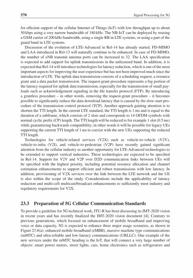
Following the success of standardization and commercialization of 4G technologies, 3GPPhas become the only place where technical work for standardizing 5G technologies will takeplace. The 5G standards from 3GPP will be brought to ITU-R for official publication in 2020with the name of IMT-2020. ITU-R agreed on the timeline and process for IMT-2020 [10] asgiven in Figure 23.9. 3GPP has to finalize the standardization of 5G so that it satisfies all therequirements of IMT-2020 by the end of 2019. It must then submit the specifications of the5G standard to ITU-R at the beginning of the “IMT-2020 specifications” process.
Even though the official IMT-2020 specifications will be published only in year 2020, thereare commercial requests to deploy the first 5G system around the year 2020. It also shouldbe noted that there are various activities in the mobile industry to demonstrate the expected5G technologies, for example at the 2018 Winter Olympics in Pyeongchang, Korea and the2020 Olympics in Tokyo, Japan. In order to meet such commercial requests, it is expected that3GPP will take a phased approach for 5G standardization. The first phase of the 5G standard,which should satisfy a part of IMT-2020 requirements, will be completed in 2018 to enableearly commercial deployment around 2020. The second phase, which should satisfy all of theIMT-2020 requirements, will be finalized in 2019 for submission to ITU-R as a candidatetechnology for IMT-2020.
To satisfy the 5G requirements, there are two candidate approaches in 3GPP: the first is tocontinue enhancing LTE-Advanced technologies and the second is the introduction of a newradio access technologies. LTE-Advanced was designed to satisfy IMT-Advanced require-ments and its enhancement beyond Rel-13 may be able to meet a part of the IMT-2020 require-ments. However, further enhancements based on LTE-Advanced to meet the more demandingIMT-2020 requirements could face significant difficulties because backwards compatibilityfor coexistence with legacy UEs needs to be maintained. Therefore, 3GPP will standardize anew radio access technology for IMT-2020.
One of the most promising technologies for the new RAT to satisfy the drastically increaseddata rate requirements of providing 20 Gbps is the utilization of higher frequency bandsthan used in traditional cellular communication bands, say around 30 GHz. Utilization ofsuch higher frequency bands make it easier to use a very wide contiguous spectrum ofbandwidth – more than 500 MHz – which would be difficult to operate by carrier aggregationas is done in LTE-Advanced. It is also a common understanding that there is not sufficientfrequency spectrum available below 6 GHz even though WRC-15 discussed allocaiton ofadditional frequency bands below 6 GHz. Due to the above considerations, there is high

�
� �
�
572 Signal Processing for 5G
(a) Usage scenarios of IMT for 2020 and beyond
IMT-2020
IMT-Advantage
(b) Enhancement of key capabilities from IMT-Advanced to IMT-2020
Enhanced Mobile Broadband
Future IMT
Ultra-reliable and low latency
communications
Massive machine type
communications
3D video, UHD screens
Peak data rate
(Gbit/s)
User-experienced
data rate
(Mbit/s)
10020
10
10
100x
3x1x
500400
350
10
10x
0.11
1
1x
1106
105
Spectrum
efficiency
Mobility
(km/h)
Network
energy efficiency
Latency
(ms)
Connection density
(devices/km2)
Area traffic
capacity
(Mbit/s/m2)
Work and play in the cloud
Augmented reality
Industry automation
Mission critical application
Self driving car
Gigabytes in a second
Smart home/Building
Voice
Smarty city
Figure 23.8 Usage scenarios and key capabilities of IMT for 2020 and beyond [4]
level of interest in utilizing the new spectrum resource above 6 GHz, not only from mobileindustries but also from governments and regional spectrum-related organizations. Therefore,it is expected that new frequency bands above 6 GHz will be allocated by WRC-19.
3GPP is expected to develop the new RAT standard to meet the IMT-2020 requirements,utilizing all frequency resources available in the traditional cellular frequency bands below6 GHz as well as high-frequency bands above 6 GHz (up to 100 GHz). It is believed thatthe OFDM-based waveform will still be a baseline waveform, with potential variations, forexample the application of additional filtering per subcarrier or per subband to reduce the
�
� �
�
5G Standard Development: Technology and Roadmap 573
IMT
-20
20
Feb.
2016
Feb.
2017
Requirement
Oct.
2017
Proposals
Evaluation criteria
Oct.
2018
Jun.
2019
Feb.
2020
IMT-2020
specifications
Oct.
2020
Jun.
2017
Evaluation
Oct.
2019
Figure 23.9 Timeline and process for IMT-2020
overhead caused by cyclic prefix and guard bands [11–16]. In order to support such a widerange of frequency bands, there will be a need to introduce multiple numerology sets defin-ing OFDM-based waveforms. For example, the subcarrier spacing in the 2-GHz frequencyband and the 30-GHz frequency band will have to be different, since the 15-kHz subcarrierspacing of the LTE standard is too narrow to be robust against RF phase noise in a frequencyband around 30 GHz. The maximum bandwidth of a carrier and the supportable FFT size willalso be reasons for defining different numerologies to support different frequency bands up to100 GHz. Even though multiple numerologies will be introduced, it will be highly desirableto keep commonality and scalability for operations in different frequency bands so that theimplementation complexity can be kept reasonable.
One of the main challenges for utilizing high-frequency bands around 30 GHz – known asthe mmWave band – is the limited coverage due to large path loss. The conventional assump-tion is that the path loss is proportional to the frequency squared. However, the utilization ofbeamforming is quite useful to improve coverage. Furthermore, it is easy to have large beam-forming gains in the mmWave band, since the wavelength becomes shorter as the frequencyincreases and there can be more antenna ports for the same antenna dimension, thereby allow-ing for sharper beams with higher beamforming gains. In the mmWave bands, conventionaldigital beamforming may not be feasible, since too many RF chains, each of which is used foreach digital path, are required to support the massive number of antenna elements. In order tokeep a reasonable RF complexity, a combination of analog beamforming and digital precod-ing – the hybrid beamforming illustrated in Figure 23.10 – is considered a practical approachfor mmWave-based systems [17–19]. The analog part forms a set of beams to make sure thatthe terminals in the coverage area can be connected to the network and the digital part canbe used to optimize performance of communication with scheduled terminals by combininganalog beams.
It is expected that the new RAT may not provide full coverage in the early phases of 5Gcommercialization. In the case of mmWave band systems, even though the beamforming willhelp increase coverage, it may not be practical to assume that full coverage can be provided.This understanding motivates the utilization of LTE-Advanced and the idea that 4G base sta-tions will give a coverage layer providing control-plane operations, while 5G base stationsserve as the capacity layer – the user-plane operation – providing high data-rate services. Thisis shown in Figure 23.11, where a terminal is simultaneously connected to both 4G and 5Gbase stations when it is in the coverage area of a 5G base station. In order to guarantee proper

�
� �
�
574 Signal Processing for 5G
IFFT DAC
Array Ant.
RF chains
P/S
IFFT DAC
P/S
MIM
O E
ncoder
Baseband Precoder
MIMOChannel
PA
a
Phase shifters
Mixer
Digital PrecodingAnalog beamforming
Figure 23.10 Hybrid beamforming
Figure 23.11 Tight integration between 4G and 5G
communication links between the terminals and the network with such split structure, it wouldbe essential to have tight integration between 4G and 5G base stations. It is noted that if the5G system supports full coverage, loose interworking with the 4G system may be enough.
A possible phased approach to support early commercial deployment around 2020 wouldbe that eMBB is optimized in the first phase and the other usage scenarios are introduced oroptimized in the second phase. In order to guarantee smooth migration from the first to thesecond phase, the first phase standard should guarantee easy and efficient introduction of newfunctions in the second phase and later. Provisioning of such forward compatibility is quiteimportant, since it is becoming more difficult to predict what services will be needed in thefuture, as the information technology is evolving. A practical way to achieve this goal wouldbe to leave as much air resource vacant as possible in the new RAT; in other words, signals andchannels should be transmitted only when needed to serve for communication for a specificterminal(s). For example, transmission of periodic signals such as the CRS of LTE system,

�
� �
�
5G Standard Development: Technology and Roadmap 575
LTE
5G
Reference signals are transmitted only within data channels
CRS is always transmitted
CRS in LTE Reference signal in 5G
Figure 23.12 An example of forward-compatible design
which makes it difficult to introduce new features later, can be minimized in the new 5G RATas illustrated in Figure 23.12.
23.4 Concluding Remarks
In this chapter, the standards roadmap from 4G to 5G was reviewed, and major enabling tech-nologies and a more detailed roadmap of 5G standards were discussed. 5G technologies shouldbe developed to enable efficient support of enhanced mobile broadband, which has been themajor focus of previous generations, as well as new services such as massive machine-typecommunications and ultra-reliable and low-latency communications. In addition to the exist-ing cellular frequency bands up to 3.5 GHz and new bands below 6 GHz, new frequency bandsabove 6 GHz (up to 100 GHz) are expected to be important in developing 5G technologies,especially for support of eMBB.
As can be seen recently, 4G technologies are having great commercial success globally. Thisbecame possible as a result of the industry momentum created through the standardizationprocess in 3GPP, and the development of the LTE and LTE-Advanced standards, in whichglobal manufacturers and major mobile network operators participated. Based on the industryexperience with 4G, the standardization process for 5G is also expected to play a crucial rolein leading research activity in 5G technologies to commercial success.
References[1] Zhang, J.C, Ariyavisitakul, S., and Tao, M. (2012) LTE-advanced and 4G wireless communications. IEEE Com-
mun. Mag., 50 (2), 102–103,[2] 3GPP (2010) TR 36.912, Feasibility study for Further Advancements for E-UTRA (LTE-Advanced)[3] METIS (2015), ICT-317669-METIS/D8.4, METIS final project report.[4] ITU-R WP-5D (2015) Document 5D/TEMP/625-E, IMT Vision – Framework and overall objectives of the future
development of IMT for 2020 and beyond[5] 3GPPTR 36.819 (2011) Coordinated multi-point operation for LTE physical layer aspects.[6] 3GPP (2014) TR 36.873, Study on 3D channel model for LTE.[7] 3GPP (2015) TR 36.897, Study on elevation beamforming/full-dimension (FD) MIMO for LTE.[8] 3GPP (2015) TR 36.889, Study on licensed-assisted access using LTE.[9] 3GPP (2013) TR 36.888, Study on provision of low-cost machine-type communications (MTC) user equipments
(UEs) based on LTE.[10] ITU-R (2015) WP-5D, Att. 2.12 to 5D/1042, ITU-R Working party 5D structure and work plan.

�
� �
�
576 Signal Processing for 5G
[11] Chang, R. (1966) High-speed multichannel data transmission with bandlimited orthogonal signals. Bell Sys.Tech. J., 45, 1775–1796.
[12] Saltzberg, B. (1967) Performance of an efficient parallel data transmission system. IEEE Trans. Commun. Tech.,15 (6), pp. 805–811.
[13] Hirosaki, M.B. (1981) An orthogonally multiplexed QAM system using the discrete Fourier transform. IEEETrans. Commun., 29 (7), 982–989.
[14] Farhang-Boroujeny, B. (2011) OFDM versus filter bank multicarrier. IEEE Signal Process.Mag., 28 (3), 92–112.[15] Premnath S. Wasden, D., Kasera, S., Patwari, N., and Farhang-Boroujeny, B. (2013)Beyond OFDM: best-effort
dynamic spectrum access using filterbank multicarrier. IEEE/ACM Trans. Network., 21 (3), 869–882.[16] Bogucka, H., Kryszkiewicz, P., and Kliks, A (2015) Dynamic spectrum aggregation for future 5G communica-
tions. IEEE Commun. Mag., 53 (5), 35–43.[17] Pi Z. and Khan F. (2011)An introduction to millimeter-wave mobile broadband systems. IEEE Commun. Mag.,
49 (6), 101–107.[18] Kim C., Kim, T., and Seol, J.Y. (2013) Multi-beam transmission diversity with hybrid beamforming for
MIMO-OFDM systems, in Proc. IEEE GLOBECOM’13 Workshop, pp. 61–65.[19] Roh, W., Seol, J.Y., Park, J., Lee, B., Lee, J., Kim, Y., Cho, J., Cheun K., and Aryanfar, F. (2014) Millimeter-wave
beamforming as an enabling technology for 5G cellular communications: theoretical feasibility and prototyperesults. IEEE Commun. Mag., 52 (2), 106–113.

ComSoc Guide to Managing Telecommunication Projects. By Celia Desmond 11Copyright © 2010 the Institute of Electrical and Electronics Engineers, Inc.
CHAPTER 2
WHY IS PM IMPORTANT, ESPECIALLYIN TELECOMMUNICATIONS?
Why is it necessary and even important to use project management? People who ap-preciate and practice project management will say that it is always important to useproject management tools and techniques for projects of any level of complexity.One might then ask why they would believe this. There are many reasons.
Some of the benefits of the application of project management techniques thatare important for any project include: ensuring good teamwork and other peoplefactors, meeting the project budget and schedule, producing products and work ofthe expected quality, effectively managing project risks, ensuring that good com-munication occurs, and ending the project by delivering results that include the fullscope as originally planned. All of these things are aspects of management of a pro-ject and they are the factors that define success in any project undertaking.
For any project, there are many factors in play. First, consider the project team,comprising the group of people actively working to deliver the product or servicethat the project is in place to produce. The project team is generally a multidiscipli-nary group; the people on the team will have different backgrounds, different objec-tives, and different ways of thinking. To ensure that such a diverse group can pro-duce whatever is required will take some management focus, and that focus is oneof the most important aspects of project management.
TEAM DIVERSITY
The team will also usually be temporary, composed of people who do not usuallywork together. Thus, it is very likely that they do not know each other well, creatinga need for time and effort to be used to develop understanding of other team mem-
c02.qxd 7/13/2010 1:19 PM Page 11

bers, to ensure that people will understand what is needed to work with the othermembers of the team. Given the multidisciplinary aspects of the project team, wecan see that considerable management effort will be needed to understand the di-verse points of view of the people assigned to the project, building a team that willwork together well and with effective communication to achieve the project goals.Again, this skill is part of project management.
In any project, the people on the team need to evaluate their own environment,their own project, their own skills, and their own company. Based on factors such asthese, they can decide how they can best work with the rest of the team to producethe best quality product or service possible.
RESOURCE LIMITATIONS
Another characteristic of projects is that there are usually hard limits to the budgetand other resources required to implement the project. Thus, there will be a need toprioritize just how and on which components the money should be spent, which isagain a component of project management.
TIME CONSTRAINTS AND LIMITATIONS
Time is always an important factor for the project manager. Since projects take peopleaway from their regular jobs, there will be time pressure to return the people to theirown organizations, even when there is little time pressure to make the project’s prod-uct or service available by a specific time. However, most projects start with scheduleconstraints already in place, so time management, another key component of projectmanagement, is also a crucial skill. Any team will be better equipped to meet both timeand cost targets if these are clear, reasonable, understood, and well communicated.
RISK MANAGEMENT
The understanding and management of risks is crucial to the project manager. Con-sidering all of the above factors of the project environment—people working withothers they do not know on multidisciplinary teams to produce something that isinitially not well defined and outside the normal work framework, with time andmoney pressure—would it be reasonable to expect that the environment for anyproject is not risky? Obviously, skill in risk management is always needed.
ENSURING QUALITY
What about quality? Projects are undertaken to take advantage of business and tech-nology opportunities to introduce a new product or service. In most cases, a new
12 2 WHY IS PM IMPORTANT, ESPECIALLY IN TELECOMMUNICATIONS?
c02.qxd 7/13/2010 1:19 PM Page 12

product or service displaces something else that had previously met the needs of thetargeted market. The quality of the new product or service is often the factor thatwill allow it to compete well with the previously established competing product orservice. To make the new product or service of the best possible quality, it shouldbe produced using quality-management techniques. Quality management, therefore,is another important aspect of project management.
SCOPE DEFINITION
One of the most important aspects of project management is the understanding,clear definition, and effective management of the project scope. Consider the natureof a project, which is to produce something unique. The output of a project is oftennot something that people already know and understand. In the case of ongoingwork in a normal production environment, it could be quite reasonable to expectthat people understand what needs to be done and what is to be produced. But at theoutset of a project, it is very likely that no one except possibly the project sponsorand the project manager has a very good understanding of what is to be produced,let alone how to achieve this. In most cases, quite a lot of work is required to clear-ly define the required output and the work needed to allow this to be provided.Scope definition and subsequent management is a large part of project manage-ment.
One of the Project Management Institute project management process areas isscope management, and within this area there are processes and tools that are usedto clearly define the scope of the project and to manage proposed changes. It takesjust common sense to realize that any project team can avoid mistakes by ensuringthat all those involved with the project, either as workers, managers, or receivers ofthe product, have a common understanding of what it is that the project will deliver,and it would be even better if they all had the same understanding of how the pro-duction of this end product would be done.
Once the project scope has been defined and approved, and the rest of the plan-ning has been done, project implementation begins. At that point, the scope, theteam, the schedule, the budget, and other project parameters have been set. Afterthis point, if changes are needed, there is potential for this change to impact manyaspects of the project. Such proposals for change are called scope changes. Therehas never been a project that did not have changes to scope. Some huge projectshave experienced literally thousands of changes to scope. For the most part, peopledo not propose scope changes for the sake of the change itself; there is generallygood reason for wanting the change. And in some cases, it makes much more senseto implement the change than to not go ahead with it. But, making any change im-pacts the project, and too many of these can cause a project to fail, no matter howwell everything else is done.
Scope change requests come in many forms. In one form, someone (usually thecustomer) says, “Just add this little feature. It only costs a little bit more, takes a lit-
SCOPE DEFINITION 13
c02.qxd 7/13/2010 1:19 PM Page 13

tle more time, and everything will be 100 times better.” That might be true and itmight well be much better to incorporate the small change now, while there are peo-ple geared up, equipment in place, and so on, than to go ahead without doing it andtry to incorporate it later, outside of the project. It might be possible to do one, ortwo, or three such additions that will cost little in time and/or money, but when thenumber of these requests gets to ten or a hundred, there is no way within the timeframe and budget, and with the people on the project team, that these can be accom-plished.
Let us be ultraconservative and suppose that each proposed scope change wasaccepted and the time required to complete each one was only one person-hour.Most people will think, rightly, that expecting each request for change to take onlyone person-hour to implement is unrealistic, as scope changes often take weeks ormonths to accommodate. But for this example, suppose each one only took onehour. If we had 1000 requests for “tiny” changes, which is not really unexpected in,say, a project with a team of 50 people running for, say, 18 months, accepting all ofthese requests would mean adding 1000 person-hours to that project. That’s an ad-dition of 125 eight hour days to the project, or more than an additional four-personmonths. And if this project received three times this many requests, which is not allthat unusual in some environments, we would need an additional person-year tocomplete just the things that were not in the initial plan if none of them took morethan one hour to complete. But of course, most take far more than a short time tocomplete, and every project receives these requests, usually many of them, so thereneeds to be some time included somehow to do these unplanned items.
Therefore, in order to be able to meet the schedule and the budget, it is necessaryto incorporate some mechanisms that will allow the project team to deal with themany change requests that will inevitably arrive. These need to be considered, as-sessed, and either accepted or rejected, and, regardless of the decision, the impactsof that decision must be dealt with. All of this will take time, and time costs money.So a change request process is a very important component of project management,and one which is needed for every project.
In another situation, the change request arrives via a statement from one of theteam members that there is a design flaw in the project or the product to be produced,and unless this is fixed the whole project will be down the drain. It just will not work.This is quite different from someone thinking up a new addition that would be nice tohave. This one, if the requestor is correct, is necessary if the project is to be success-ful. But it is still a change to the project scope, and making the change will cost timeand money, not to mention the possibility of needed additional skills or a new risk tothe team. The change must be accepted, but this should not be done lightly. Good pro-ject management practice requires that this proposed change go through the changerequest process, and if accepted, be implemented only once all the impacts are un-derstood and the required resources have been obtained.
In short, every project will experience proposals for changes to the initiallyplanned scope. And these changes do interfere with projects. A few smaller ones
14 2 WHY IS PM IMPORTANT, ESPECIALLY IN TELECOMMUNICATIONS?
c02.qxd 7/13/2010 1:19 PM Page 14

might be incorporated by having people work a little harder, or some such mecha-nism, but, overall, if you take on many changes, or large ones, the project will notfinish on time, with the right quality level of product, at the right budget. Well-de-fined project management techniques help the project manager be clear on whatfactors the team, and the project manager himself, is being measured. Quite possi-bly, one’s bonus for the year, or even keeping one’s job, depend on projects finish-ing on time, on budget, or with some specific deliverables working well. If as a pro-ject manager you keep taking on more work without ensuring that compensatingbudget or schedule changes are put in place, failure is inevitable. Every project un-dergoes scope changes; we know before the project starts that these requests are go-ing to come, so it only makes sense to plan for them.
PROJECT OBJECTIVES
Another aspect of project planning is the setting and communication of clear, at-tainable, and measurable objectives. Doing this can avoid frustration by ensuringthat the team members and the key stakeholders all march to the same drummer.A team will be better able to ensure that all those involved with the project in anyway have the same expectations and the same information if there is good com-munication, especially agreed-upon formal communication. But communicationdoes not just happen: proper communication requires planning and focus, both ofwhich are skills of the good project manager. With the right attention by all teammembers who have something useful to contribute, decisions can be made con-sciously and for the right reasons. It is part of the project manager’s role to ensurethat this will happen.
With the right communication, it is easier for the team to avoid known pitfalls,even for a fairly straightforward project. Consider the following example of orga-nizing an IEEE conference.
In a volunteer organization such as IEEE, typical projects might be the organiza-tion of conferences, whether small ones of only 50–200 attendees, or large ones at-tracting thousands of people. Such projects include the preparation of publicationswith papers by many authors; the initial request for these papers; receipt and reviewof the papers; organization of the papers into sessions with a technical theme; theorganization of meals and coffee breaks; the organization of events such as recep-tions; providing speaker instructions or awards presentations; the making of hotelarrangements, and, possibly, conference center arrangements so that attendees willhave a place to stay and sessions can be held; the publicizing of the event; and soon. Obviously, these functions are not all carried out by only one or two people, sothere is a requirement that there be good communication amongst the organizers.The rooms need to be the right size for the sessions, and the conference needs tohave enough rooms. The attendees need to have the information about the confer-ence, how to register, where it will be held, when and where to attend the sessions,
PROJECT OBJECTIVES 15
c02.qxd 7/13/2010 1:19 PM Page 15

and so on. So not only must there be good communication amongst the organizersin each area, there must be good communication amongst the organizers of the dif-ferent aspects of the conference, and excellent communication with potential andconfirmed conference attendees, to attract people and ensure that they get the mostout of the conference. The people doing the organization are all volunteers. Theywork for different companies and frequently live in different countries, yet theymust work together to make the conference happen smoothly. This can be doneonly with strong, planned, well-organized communication.
Another quite different volunteer project is our example of the CommunicationsSociety Wireless Communications Engineering Technologies Certification, forwhich the team has over 100 members. This project again has not only a large team,but people working in very diverse areas and roles within the project, and these peo-ple live in over 20 countries around the world. Although it is not necessary for eachof these people to communicate directly with all of the others, it is clear that the cer-tification cannot be developed efficiently or successfully without strong, planned,organized communication amongst the team members, and a great deal of it, for asuccessful outcome. In volunteer work, project teams are made up of people whowork for companies, self-employed entrepreneurs, and academics, who frequentlylive in many different countries around the world. These people agree to do the vol-unteer work in addition to their own workload, for no monetary compensation. Theproject manager does not have any control over the people in a volunteer organiza-tion. These people are working on the project because they want to be there, and ifthey do not feel like providing their deliverables until the last minute or submittinga status report, they do not have to. And unless the project manager can influencethe people positively, some of the material needed for the project will not meet re-quirements. Today, similar situations often exist in electronic communications pro-jects within for-profit companies. The team members are not volunteers, but theymay be working in environments that are as diverse as those described here andthey could well also work for different companies that are cooperating to build ajoint product or service.
Managing projects for volunteer work is different from doing so at work, wherethe project manager has a degree of defined authority. But even in work situationsin which project managers have control over all the people on their teams, generallythey do not have control at all over most of the project stakeholders. Project man-agers do not always directly supervise the people that are working on the project. Insome management structures, the project manager is more of a coordinator, anddoes not directly supervise any of the team members. The team members continueto report to their usual supervisors, but are assigned project work instead of, or inaddition to their regular job. The project manager is charged with overseeing theproject work and making sure that it all happens according to the project needs andplan. That means that it is up to the project manager to use relevant skills, not thelimited authority associated with the project manager title, to get people to dothings, to get them done well, and to get them done on time.
16 2 WHY IS PM IMPORTANT, ESPECIALLY IN TELECOMMUNICATIONS?
c02.qxd 7/13/2010 1:19 PM Page 16
WHAT ABOUT TELECOM PROJECTS?
The title of this chapter emphasizes the importance of project management fortelecommunications projects. So far, the discussion has been about the importanceof project management for projects in general, with no specific reference totelecommunications projects. This book focuses on the application of project man-agement principles to telecommunications-related projects. It is more important touse proper project management technique in telecommunications than in most othersectors due to some particular characteristics of the industry.
Consider the type of projects that typically occur in the telecom industry. Manyof these involve huge networks, either for a provider or a large end user, or ex-tremely complex services and equipment, with hardware, software, business, andintegration aspects. Teams tend to be large—from 25 to hundreds of people per pro-ject—and the technologies involved are extremely complex. Project managementlends itself well to handling such size and complexity. Most significantly, in thisrapidly changing industry, many companies find themselves needing to do thingsfor the first time, and handling these situations by implementing projects is oftenthe only practical way of accomplishing this.
Telecommunication technologies involved in projects are usually fairly new (and,therefore, not well known), and there is a requirement in many cases for interworkingof many different technologies. All of this creates a requirement for significant tech-nical knowledge on the team, and, generally, also significant business or marketingknowledge, making it necessary that the teams be multidisciplinary and competingfor people with scarce and valuable skills and experience. The application and inter-working of new technologies ensures that telecom projects will contain a higher thanaverage degree of risk. This unpredictability implies that there will be challenges indefining the project scope accurately, in turn making timelines and budgets hard tonail down. All of this adds up to a need for strong and ingenious project management.
Telecom projects are planned and implemented in an environment that experi-ences continuous, significant, and rapid changes. The following is a view of severalaspects of the telecommunications industry that are important to the application ofproject management in this sector.
Technologies
Whether we look at access, transmission, switching, terminal devices, service plat-forms, servers, billing, provisioning, ordering testing, or any aspect of telecommu-nications products or services, we find very many technologies in use. These are atvarious stages of development, and they all must interwork with each other andwith applications that customers create, such as local area networks. Consider ac-cess technologies. These could include copper pairs, video cable, wireless, or fiberoptics. And if we take just one of these technologies, say wireless, there are proba-bly no less than 15 different versions of this technology that might come into play
WHAT ABOUT TELECOM PROJECTS? 17
c02.qxd 7/13/2010 1:19 PM Page 17

in some way in a project, including WiFi, WiMax, satellite, Bluetooth, and ultrawideband. Some projects do not involve more than one of these, while others mightinvolve many. But almost all telecom projects do include at least one relatively newand rapidly evolving technology, resulting in an unstable project environment.Thus, there is a very great need for technical skills that must be developed and keptcurrent as the project evolves, placing more stress on the project than there is in oth-er industries in which the technologies are less complex and more static.
Services
In this book, we discuss the changing nature of the services offered today, as the In-ternet and entertainment media become integral to electronic communications ser-vices. Whereas for many years a telecom service involved mainly local voice ser-vice or long distance voice service, with possibly a separate data component,today’s services need to be built by integrating voice, data, and multimedia in inno-vative ways in order to be successful. The requirements for such projects are muchmore complex than they have been in the past for telecom services, since the needfor innovation creates higher risks, as does the integration of the many differentcomponents. Customer expectations of new services are escalating very rapidly.Capabilities that were considered close to miraculous five years ago are now con-sidered outdated and of little interest. It is extremely difficult, despite the efforts ofarmies of marketers, to predict what service will be a hot item months in the future.So the risk is high, and the teams of people from many different areas must work to-gether in order to introduce successful service offerings.
Companies in the Business
In the previous chapter, we talked about the rate at which competition is escalatingin electronic communications and the many different companies that are now pro-viding these services. Projects are put in place to either take advantage of opportu-nities or create solutions to problems. These opportunities and problems occur in anenvironment that is ever changing, where competing companies may create marketor operational pressures that impact the project, the project work, and the projectoutputs. If the home company of a project merges or becomes acquired, the natureof the project is often affected. When a new competitor appears with products thatare new, better, or different, priorities of the project change. So the evolution of thecompanies in the relevant business sector places a heavy strain on the project teamsworking to provide services and products for telecommunications.
Regulatory Environment
Over the past 10–20 years, the level of regulation governing telecom has been grad-ually decreasing in most areas. However, many things are still regulated, and some
18 2 WHY IS PM IMPORTANT, ESPECIALLY IN TELECOMMUNICATIONS?
c02.qxd 7/13/2010 1:19 PM Page 18
are heavily controlled. Once regulations are set and understood, they place require-ments on the project that must be incorporated into the project requirements alongwith any other requirements. Project teams often need to work during intervalswhen regulatory changes are expected or threatened, without knowing what the sit-uation will be at some point in the future. This greatly increases the project risk, andalso the stress on the project team, creating a need to manage toward the most opti-mal solution.
Successful Business Model
Since the inception of the telecom technologies and business, the industry has oper-ated under similar business models in most countries. These business models havebeen based on the premise that the customer pays for the service delivered. Some-times the models were usage based, and in other cases the payments were flat rates,usually monthly. In some cases, the customer pays for both outgoing and incomingcalls, whereas in other cases only outgoing calls are charged. When there is a needfor equipment beyond that used for standard service, the customer might eitherlease or purchase the additional equipment. Today, for many services these tradi-tional models do not apply. Instead, the services are sometimes offered free, withadvertisers paying the cost, with rates depending on the popularity of the services.Thus, in addition to the need for more innovation in the development of new ser-vices, the teams often also have to deal with a new business model. This againmakes the environment more risky, increasing the need for good project manage-ment.
Internal Corporate Structures
Yet one more issue that teams face during today’s projects is the internal restructur-ing of their companies, moving from highly hierarchical structures to ones that areflatter, or from structures based on older services such as local, long distance, andcellular to structures based on models of newer services, such as video or social net-working. The team then is essentially standing on a rolling platform while theywork on the project. This raises the stress level of the people on the team, including,of course, the project manager. People will dilute their focus on the project as theywatch the developments in their company, increasing the pressure for the manage-ment of the project.
Customers
Given that competition is rampant today, customers have to deal with more choicesand the anxieties they bring with them. They do not know with any certainty whichcompany to buy from or which offer to take. If the project is providing a product orservice for outside customers, there is a need that is becoming more important for
WHAT ABOUT TELECOM PROJECTS? 19
c02.qxd 7/13/2010 1:19 PM Page 19
telecom projects—that of understanding the perspective of the potential customersand even determining what emerging entity might become a potential customer.This is an increase in the scope of projects above that experienced in this industry inthe past requiring new skills and teams to deal with new perspectives. This, in turn,creates more need for team building, for clear understanding of the project scope,and for communication of this changing information to the project team. All ofthese are again components of the project manager’s job.
The Best Way to Market
Customer needs are changing, as are business models. Even the types of servicesand products that should be offered are not what they used to be. There is also aneed to for the project team to understand how to build marketing plans, and how tobest approach the market. This again extends the skills needed and the number ofperspectives the team must consider.
Service Models
Telephone services have been highly controlled in the past, in the sense that the in-telligence that makes the service work, and the control of the network, its traffic,and all of its operating parameters have been all completely in the hands of the pro-viding company. Traditional companies are very protective of these services, andtheir control, but this way of doing things is becoming less dominant in the telecomindustry. Newer services use open platforms, and often contain components provid-ed and built by multiple providers. Network intelligence and control is no longersolely resident in the core of the network and, in fact, much of the control resides atthe edge. Rather than a service being delivered in its entirety by a single serviceprovider, it is now often delivered by a loose partnership of specialized companies.This, of course, increases the risk that the service will not work well, and the pres-sure on the architects of the network to know, understand, and work with multipletechnologies and providers. Again, this is one more pressure on the project, and onemore reason that management is needed.
Network Architecture
In the previous chapter, we discussed the evolution of telecom networks from cir-cuit-switched systems connected via TDM facilities to packet-switched networksrunning Internet Protocol. This change of the technical environment in which newprojects are implemented from that which many team members know drives a needfor constant learning on the part of the team members to keep current. Inability todo so reduces the technical effectiveness of the team, adds risks due to the higherprobability of wrong decisions arising from unfamiliarity with the technology, andalso can seriously impair the self-confidence of the team members, leading to per-
20 2 WHY IS PM IMPORTANT, ESPECIALLY IN TELECOMMUNICATIONS?
c02.qxd 7/13/2010 1:19 PM Page 20

sonal stress and highly risk-averse behavior. Identification and implementation ofthe necessary training should be a factor in the planning of the project.
CONCLUSION
It is clear that the skills, technical and otherwise, required to effectively complete atelecom project today are more varied than those that have been needed in the past.Summing up all of the variables discussed in this chapter and in the previous one,we see that many, many things are evolving and changing, and the sum of all thesechanges is a very volatile environment in which to do projects. Because of the de-gree of change encountered in the telecommunications industry, the need for projectmanagement is much greater than in many other sectors. Electronic communica-tions project teams are operating with a high degree of change in many areas, andthese must be well understood when planning, designing, and implementing pro-jects:
� Changing business environment
� Increased level of competition
� Accelerated project schedules
� Unfamiliar new technologies
� New business models with integration aspects outside the control of the team
� Change-driven personal stress effects on team members and other stakehold-ers
� High costs for evolution of networks in a era of tight budgets
� Importance of communications is escalating a core process for project teams
Some degree of project management is needed for any project, and the morecomplex the project, the greater the need for the management and the more formalthe processes become. Telecom projects are more complex by far than most otherprojects, and they are also generally larger. Both of these factors increase the de-mand for project management in order to enhance project success. Projects in tele-com occur today in environments dealing with rapid change, and many widely dif-ferent aspects of the project environment are changing as the projects proceed. Evenone of these changes would be significant justification for strong management ofprojects. But in the electronic communications environment, many of these diversechanges are operating in parallel, so if project management is needed anywhere, itis needed desperately in today’s telecommunications industry.
CONCLUSION 21
c02.qxd 7/13/2010 1:19 PM Page 21

JWBS201-c10 JWBS201-Blume October 27, 2016 15:57 Printer Name: Trim: 6.125in × 9.25in
CHAPTER 10PERSONAL PROTECTION(SAFETY)
CHAPTER OBJECTIVES
After completing this chapter, the reader will be able to:
✓ Discuss “Personal Protection Equipment” used for safety in electric powersystems
✓ Explain human vulnerability to electricity
✓ Explain how one can be safe by “Isolation” or “Equipotential”
✓ Discuss “Ground Potential Rise” and associated “Touch” and “Step” poten-tials
✓ Discuss how “Energized” or “De-energized and Grounded” lines provide safeworking environments for field workers
✓ Discuss the “Safety Hazards” around the home
ELECTRICAL SAFETY
The main issues regarding electrical safety are the invisible nature of hazardous situ-ations and the element of surprise. One has to anticipate, visualize, and plan ahead forthe unexpected and follow all the proper safety rules before an accident to gain con-fidence in working around electricity. Those who have experience in electrical safetymust still respect and plan for the unexpected. There are several methodologies andpersonal protective equipment (PPE) available that make working conditions aroundelectrical equipment safe. The common methodologies and safety equipment areexplained in this chapter. The theories behind those methodologies are also discussed.Having a good fundamental understanding of electrical safety principles is veryimportant and is effective in recognizing and avoiding possible electrical hazards.
There are two aspects of electrical safety that are discussed in this chapter;electric shock or current flow through the body and arc-flash or being burned by theheat created by an electrical arc when equipment failure occurs. Protection againstelectrical shock is discussed first.
Electric Power System Basics for the Nonelectrical Professional, Second Edition. Steven W. Blume.© 2017 by The Institute of Electrical and Electronics Engineers, Inc. Published 2017 by John Wiley & Sons, Inc.
209

JWBS201-c10 JWBS201-Blume October 27, 2016 15:57 Printer Name: Trim: 6.125in × 9.25in
210 ELECTRIC POWER SYSTEM BASICS FOR THE NONELECTRICAL PROFESSIONAL
PERSONAL PROTECTION
Personal protection refers to the use of proper clothing, insulating rubber goods orother safety tools that provide electrical isolation from electrical shock. Another formof personal protection is the application of equipotential principles, where everythingone comes in contact with is at the same potential. Electrical current cannot flowif equipotential exists. Either way, using insulating personal protection equipment(PPE) or working in a zone of equipotential are known methods for reliable electricalsafety.
Human Vulnerability to Electrical Current
Before discussing personal protection in greater detail, it is helpful to understandhuman vulnerability to electrical current. The level of current flowing through thebody determines the seriousness of the situation. Note, the focus is on current flowthrough the body opposed to voltage. Yes, a person can touch a voltage, create a pathfor current to flow, and experience a shock, but it is the current flowing through thebody that causes issues.
Testing back in the early 1950s showed that a range of about 1–2 mA (0.001–0.002 A) of current flow through the human body is considered the threshold of sensi-tivity. As little as 16 mA (0.016 A) can cause the loss of muscle control (lock-on). Aslittle as 23 mA (0.023 A) can cause difficulty breathing, and 50 mA can cause severeburning. These current levels are rather small when compared to normal householdelectrical load. For example, a 60 W light bulb draws 500 mA of current at full bright-ness with rated voltage of 120 V.
The residential ground fault circuit interrupter (GFCI) like those used in bath-rooms (discussed earlier) open the circuit if the differential current reaches approxi-mately 5.0 mA (0.005 A). The GFCI opens the circuit breaker before dangerous cur-rent levels are allowed to flow through the human body. The conclusion is humansare very vulnerable to relatively small electrical currents.
Principles of “Isolation” Safety
A person can be safe from electrical hazards through the use of proper rubber isola-tion products, such as gloves, shoes, blankets, and mats. Proper rubber goods allow aperson to be isolated from touch and step potentials that would otherwise be danger-ous. (Note, touch and step potentials are discussed in more detail later in this chapter.)Electric utilities test their rubber goods frequently to insure that safe working condi-tions are provided.
Rubber gloves are routinely used when working on de-energized high-voltageequipment just in case it becomes accidently energized. Rubber gloves are also usedfor hot-line maintenance at distribution voltage levels only. Figure 10-1 shows thecotton inner liners, insulated rubber glove, and leather protector glove used in typ-ical live line maintenance on distribution systems or to protect against accidentalenergization.

JWBS201-c10 JWBS201-Blume October 27, 2016 15:57 Printer Name: Trim: 6.125in × 9.25in
PERSONAL PROTECTION (SAFETY) 211
Figure 10-1 Rubber gloves. Courtesy of Alliant Energy.
Figure 10-2 shows high-voltage insulated boots. Figure 10-3 shows typicalhigh-voltage insulated blankets and mats. Every electric utility has extensive andvery detailed safety procedures regarding the proper use of rubber goods and othersafety-related tools and equipment. Adherence to these strict safety rules and equip-ment testing procedures insures that workers are safe. Further, electric utilities spendgenerous time training workers to work safety, especially when it comes to live lineactivities.
Principles of “Equipotential” Safety
Substations are built with a large quantity of bare copper conductors and ground rodsconnected together and buried about 18–26 inches below the surface. Metal fences,
Figure 10-2 Insulated boots.

JWBS201-c10 JWBS201-Blume October 27, 2016 15:57 Printer Name: Trim: 6.125in × 9.25in
212 ELECTRIC POWER SYSTEM BASICS FOR THE NONELECTRICAL PROFESSIONAL
Figure 10-3 Rubber blankets and mats. Courtesy of Alliant Energy.
major equipment tanks, structural steel, and all other metal objects requiring an elec-trical ground reference are all connected to the buried copper conductors. This elabo-rate interconnected system of conductive metals form what is referred to as the stationground grid.
This elaborate ground grid provides a safe working environment that is some-times referred to as equipotential grounding. Usually a copper conductor is buriedoutside the fence perimeter (approximately 3 feet from the fence) to extend the groundgrid for additional safety. Usually 2–4 inches of clean gravel is placed on top of thesoil in the substation to serve as additional isolation from current flow and voltageprofiles that could exist in the soils during fault conditions. Figure 10-4 shows theground grid concept.
There are two main reasons for having an effective grounding system; first,to provide a highly effective ground path through earth soil for fault current to flowback to the source in order to trip circuit breakers (i.e., system protection). Second,effective grounds provide a zone of equipotential for safe working environments (i.e.,personnel protection). The effective ground grid causes high fault currents to trip
Lightning
or power fault
Lightning rods
Ground rodsGround grid wires
Figure 10-4 Substation ground grid.

JWBS201-c10 JWBS201-Blume October 27, 2016 15:57 Printer Name: Trim: 6.125in × 9.25in
PERSONAL PROTECTION (SAFETY) 213
Ground potential rise
Ground grid
Figure 10-5 Substation ground potential rise.
circuit breakers faster. The zone of equipotential minimizes the risk of someone expe-riencing a current flow during a lightning strike or power fault. Theoretically, every-thing a person touches in a zone of equipotential is at the same voltage and thereforeno current flows through the person. As an example, suppose you were in an airplaneflying above the earth at 30,000 feet. Everything inside the airplane seems normal.The same is true in a properly designed substation when a 30,000 V ground potentialrise occurs.
Ground Potential Rise
When a fault occurs on a power system, a ground potential rise (GPR) conditionoccurs where high electrical currents flow in the earth soil creating a voltage profile onthe earth’s surface. This voltage profile decays exponentially outward from the faultlocation as shown in Figures 10-5 and 10-6. This GPR condition can cause dangeroustouch and step potentials.
The following drawings show the GPR and touch and step potentials.
Touch Step
Distance from fault
Figure 10-6 Touch and step around structures.

JWBS201-c10 JWBS201-Blume October 27, 2016 15:57 Printer Name: Trim: 6.125in × 9.25in
214 ELECTRIC POWER SYSTEM BASICS FOR THE NONELECTRICAL PROFESSIONAL
Touch and Step Potentials
During a lightning strike or power fault event in a substation, the entire substationrises to a high potential and anyone standing on the ground grid during that eventshould experience no touch or step potential because of the equipotential ground-ing. Touch potential is the difference between the voltage magnitude of a person (oranimal) touching an object and the magnitude of voltage at the person’s feet. Touchpotential can also be the difference in voltage between two potentials (i.e., hand tohand). Step potential is the difference in voltage between a person’s (or animal’s)feet. Shoes, gloves, and other articles of clothing help insulate a person from touchand step potentials. Approved, tested, and properly used rubber safety products (PPE)provide isolation from potentially hazardous touch and step potentials.
Working Transmission Safely
Construction and maintenance crews work on power lines under-energized and de-energized conditions. Either way, special safety precautions are mandatory. All safetyprecautions fall back to the basic principles of either being fully isolated from electricshock or be in a zone of equipotential. One has to plan on the possibility of a de-energized line becoming accidently energized without notice. Following are examplesof different ways to work on power lines safely.
Energized EquipmentThere are multiple ways to work on energized power lines safely; insulated buckettrucks, the use of fiber glass non-conductive hot sticks and bare hand live line main-tenance are the more common means.
Insulated Bucket Trucks Working out of insulated bucket trucks is a meansof working on lines that are either energized or de-energized.
Depending on the system voltage being worked on, rubber gloves, fiber glasshot sticks, or live line bare hand methods can be used safely by working out of insu-lated trucks. Figure 10-7 shows using an insulated truck
Hot Stick Live Line Maintenance Work can be performed when the lines areenergized using hot sticks. Figure 10-8 shows workers using fiberglass hot sticks toperform maintenance.
“Bare Hand Live Line” Maintenance A person can be placed in a conductivesuit and touch energized transmission voltages as shown in Figure 10-9 as long as theydo not come in contact with grounded objects. This is like a bird sitting on the wire.The conductive suit establishes a zone of equipotential and thus eliminates currentflow inside the suit or human body. Since everything the person touches is at the samepotential, no current flows through the body and the person is safe from electricalshock. (Picture of author touching live 345 kV)
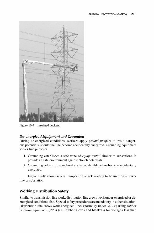
JWBS201-c10 JWBS201-Blume October 27, 2016 15:57 Printer Name: Trim: 6.125in × 9.25in
PERSONAL PROTECTION (SAFETY) 215
Figure 10-7 Insulated buckets.
De-energized Equipment and GroundedDuring de-energized conditions, workers apply ground jumpers to avoid danger-ous potentials, should the line become accidentally energized. Grounding equipmentserves two purposes:
1. Grounding establishes a safe zone of equipotential similar to substations. Itprovides a safe environment against “touch potentials.”
2. Grounding helps trip circuit breakers faster, should the line become accidentallyenergized.
Figure 10-10 shows several jumpers on a rack waiting to be used on a powerline or substation.
Working Distribution Safety
Similar to transmission line work, distribution line crews work under-energized or de-energized conditions also. Special safety procedures are mandatory in either situation.Distribution line crews work energized lines (normally under 34 kV) using rubberisolation equipment (PPE) (i.e., rubber gloves and blankets) for voltages less than

JWBS201-c10 JWBS201-Blume October 27, 2016 15:57 Printer Name: Trim: 6.125in × 9.25in
216 ELECTRIC POWER SYSTEM BASICS FOR THE NONELECTRICAL PROFESSIONAL
Figure 10-8 Live maintenance transmission lines.
Figure 10-9 Bare hand live line maintenance.

JWBS201-c10 JWBS201-Blume October 27, 2016 15:57 Printer Name: Trim: 6.125in × 9.25in
PERSONAL PROTECTION (SAFETY) 217
Figure 10-10 Ground jumpers.
usually 34 kV. Figure 10-11 shows live line maintenance activities on distributionsystems. Working lines de-energized requires “ground jumpers” as discussed earlier.
Switching
Switching is the term used to change the configuration of the electric system or toprovide isolation for safe working activities on equipment, such as maintenance.Switching is required to open or close disconnect switches, circuit breakers, etc. for
Figure 10-11 Live maintenance distribution. Courtesy of Alliant Energy.

JWBS201-c10 JWBS201-Blume October 27, 2016 15:57 Printer Name: Trim: 6.125in × 9.25in
218 ELECTRIC POWER SYSTEM BASICS FOR THE NONELECTRICAL PROFESSIONAL
Figure 10-12 Live maintenance substations.
planned maintenance, emergency restoration, load transfer, and equipment isolation.Figure 10-12 shows a switching event in an energized substation. Switching requirescareful control of all personnel and equipment involved. This usually requires radio,phone, or visual communication at all times for safety assurance. Detailed radio andequipment tagging procedures are also required to help prevent others from interfer-ing with work activities. Switching can be very time consuming due to the repetitivenature of the communication of the switching orders.
ARC-FLASH
Electrical arc-flash hazards are serious risks to worker safety. On the average, everyday in the United States, five to ten people are sent to special burn units due to arc-flash burns. The National Fire Prevention Association (NFPA) published NFPA 70E®,the standard for Electrical Safety in the Workplace®, in order to document electricalsafety requirements regarding arc-flash safety. 70E® defines specific rules for deter-mining the category of electrical hazards and the PPE required for personnel workingin defined and marked hazard zones or boundaries. OSHA enforces the NFPA arc-flash requirements under its “general rule” that a safe workplace must be maintained.These regulations are forcing employers to review and modify their electrical systemsand work procedures to reduce the arc-flash hazard and to improve worker awarenessand safety.
Industry regulations and standards now require the electrical equipment ownerto do the following:
� Assess whether there are arc-flash hazards� Calculate the energy released by the arc, if or when present� Determine the flash protection boundaries

JWBS201-c10 JWBS201-Blume October 27, 2016 15:57 Printer Name: Trim: 6.125in × 9.25in
PERSONAL PROTECTION (SAFETY) 219
� Provide appropriate PPE for personnel working within the flash protectionboundary
� Provide a safety program and training with clear responsibilities� Suitable tools, in addition to PPE for a safe workplace� Equipment labels indicating the minimum protective distance, the incident
energy level, and required PPE for that location
Employees too have an obligation to arc-flash safety. They must follow therequirements of arc-flash labeling by wearing the proper PPE and use proper safetytools provided by their employer. Further, they must not work on or near electricalcircuits or equipment unless they are “qualified” workers.
About the Arc
An arc-flash is the light and heat produced from an electric arc when supplied withsufficient electrical energy that can cause substantial damage, harm, fire, and/or seri-ous injury. Electrical arcs, when controlled, produce a very bright light and whencontrolled, can be used in arc lamps (having electrodes), for welding, plasma cuttingand other industrial applications.
When an uncontrolled arc forms at high voltages, arc-flashes can produce deaf-ening noises, supersonic concussive-forces, super-heated shrapnel, temperatures fargreater than the sun’s surface, and intense high-energy radiation capable of vaporizingnearby materials. Arc-flash temperatures can reach or exceed 35,000◦F (19,400◦C) atthe arc terminals. The result of the violent event can cause destruction of equipment,fire, and injury not only to an electrical worker but also to bystanders. Figure 10-13shows what happens after an arc-flash event.
Figure 10-13 Arc-flash. Reproduced with permission of from LSelectric.

JWBS201-c10 JWBS201-Blume October 27, 2016 15:57 Printer Name: Trim: 6.125in × 9.25in
220 ELECTRIC POWER SYSTEM BASICS FOR THE NONELECTRICAL PROFESSIONAL
Hazard Categories
NFPA 70E® includes hazard categories that take into account human vulnerabilityfactors and the capability of available PPE clothing used to protect humans that areexposed to arc-flash incidents. Calories/cm2 is the reference used in arc-flash criteria.One calorie/cm2 can be equal to holding your finger over the tip of a flame of acigarette lighter for one second. Specifically, one calorie is the amount of heat neededto raise the temperature of one gram of water by 1◦C. Further, thermal energy is ratedin calories/cm2. A second-degree burn requires approximately 1.2 cal/cm2 for morethan one second.
Below are the categories used in arc-flash rules and regulations. These cate-gories correspond to required PPE.
� Category 0: Up to 1.2 cal/cm2
� Category 1: 1.2–4 cal/cm2
� Category 2: 4.1–8 cal/cm2
� Category 3: 8.1–25 cal/cm2
� Category 4: 25.1–40 cal/cm2
� Over 40 cal/cm2: Unacceptable risk
Protective Clothing and Equipment
Personal protective equipment (PPE) is the common term used for clothing andequipment to protect electrical workers performing activities on or near energizedhigh-voltage equipment. In the case of exposure to arc-flash hazards and dependingon the hazard risk category (defined by NFPA), PPE is primarily made up of flameresistant (FR) clothing. FR clothing is the most common and industry accepted PPEto protect the body from burns due to flame. It is not, however, designed to isolatethe worker from electrical contact. The beneficial characteristic of FR clothing isthat it will not continue to burn on its own when a flame source is removed. Thisprotection is achieved by treating the fiber cloth with flame retardant “modacrylic”blended cottons.
Table 10-1 shows the required FR PPE required for the various hazard/riskcategories.
TABLE 10-1 Required Flame Retardant Clothing
Hazard/RiskCategory
Eye Protection, Ear CanalInserts, Long Sleeve Shirt
and Pants
ArcRated
Clothing
Face andHead
Protection
FlashSuit
Hood
0√
1√ √ √
2√ √ √
3√ √ √ √
4√ √ √ √

JWBS201-c10 JWBS201-Blume October 27, 2016 15:57 Printer Name: Trim: 6.125in × 9.25in
PERSONAL PROTECTION (SAFETY) 221
Figure 10-14 Arc-flash clothing. Reproduced with permission of from LSelectric.
In most applications, clothing and PPE must be either FR rated or arc-flashrated. The electrical worker should never wear materials such as nylon and polyesterthat can melt and stick to skin. Note non-FR-rated undergarments may catch fire evenwhen arc rated clothing is worn overtop and survives an arc-flash.
Although some of this clothing and equipment appears to be bulky, restrain-ing, and cumbersome, manufactures try hard to add flexibility, light weightiness, anddurability in their FR clothing while meeting the strict arc-flash requirements. Fig-ure 10-14 shows the clothing required for Category 4 energy.
The arc rating of the FR material is the maximum incident energy resistancedemonstrated by a material prior to break open (a hole in the material) or to passthrough and cause a second- or third-degree burn with 50% probability.
Arc rating is normally expressed in cal/cm2 (or small calories of heat energyper square centimeter). The tests for determining arc rating are defined in ASTMF1506 Standard Performance Specification for Flame Resistant Textile Materials forWearing Apparel for Use by Electrical Workers Exposed to Momentary Electric Arcand Related Thermal Hazards.
Approach Boundaries
Based on the hazard categories stated earlier and the PPE flame retardant capabilities,NFPA 70E® also stipulates four arc-flash approach boundaries that must be knownand observed. Figure 10-15 shows these approach boundaries.

JWBS201-c10 JWBS201-Blume October 27, 2016 15:57 Printer Name: Trim: 6.125in × 9.25in
222 ELECTRIC POWER SYSTEM BASICS FOR THE NONELECTRICAL PROFESSIONAL
Figure 10-15 Arc-flash boundaries.
Flash protection boundary (outer boundary) is where a worker is exposed to acurable second-degree burn if outside this boundary.
Limited approach boundary is the closest area an unqualified person can safelystand. Still requires PPE. A person must be qualified to go any closer.
Restricted approach boundary is the closest a qualified person can stand, pro-vided they have an approved plan for the work to be performed and it must be abso-lutely necessary to work in this area.
Prohibited approach boundary (inner boundary) is considered the same as mak-ing contact with the energized part. Requires qualified person with specific train-ing to work on energized conductors, appropriate PPE, and documented plan withjustification.
As you can see, electrical workers are required to work safely using proper PPEfor both electrical contact and arc-flash hazards. All industries have their hazards;the electrical industry has these two concerns. Proper training, safety equipment, andhaving the proper understanding of the hazards before a live contact or arc-flash eventoccurs provide electrical workers with the necessary situational awareness, tools, andassurance that a safe working environment is provided.
ELECTRICAL SAFETY AROUND THE HOME
Home safety also involves the awareness of touch and step potentials, arc-flash too.Whether one is exposed to a dangerous touch or step potential in a substation orat home, the same circumstances exist and the same precautions are necessary. Assoon as the insulation around energized wires is compromised, dangerous step andtouch potentials can exist, plus a bright arc-flash event can occur if and when frayedinsulated conductors touch.

JWBS201-c10 JWBS201-Blume October 27, 2016 15:57 Printer Name: Trim: 6.125in × 9.25in
PERSONAL PROTECTION (SAFETY) 223
Figure 10-16 Safety at home. Reproduced with permission of Photovault.
Figure 10-17 GFCI receptacle. Reproduced with permission of Photovault.
For example, worn extension cords can have exposed conductors that can cause120 Vac touch potential hazards. All worn cords must be replaced. To compound theproblem, water, moisture, metal objects, and faulty equipment can increase the possi-bility of injury from accidental contact. Everyone is vulnerable to electrical current,therefore always be vigilant about electrical safety at home!
Figures 10-16 and 10-17 show how electrical safety starts at home. Reproducedwith permission of Photovault.
Always be vigilant about electrical safety at home!

4Predictive Control of aThree-Phase Inverter
4.1 Introduction
Current control is one of the most studied problems in power electronics [1–3], so it isvery important to study as a first step the application of MPC in a current control scheme.In addition, the three-phase, two-level inverter is a very well-known topology that can befound in most drive applications.
This chapter presents a MPC scheme for current control in a three-phase inverter,which is based on the control scheme reported in [4]. The control scheme and workingprinciple will be explained in more detail than other applications in this book because thesame ideas and explanations can be extended for all examples presented in the followingchapters.
4.2 Predictive Current Control
The proposed predictive control strategy is based on the fact that only a finite number ofpossible switching states can be generated by a static power converter and that models ofthe system can be used to predict the behavior of the variables for each switching state.For the selection of the appropriate switching state to be applied, a selection criterionmust be defined. This criterion consists of a cost function that will be evaluated for thepredicted values of the variables to be controlled. Prediction of the future value of thesevariables is calculated for each possible switching state and then the state that minimizesthe cost function is selected.
This control strategy can be summarized in the following steps:
• Define a cost function g.• Build a model of the converter and its possible switching states.• Build a model of the load for prediction.
Predictive Control of Power Converters and Electrical Drives, First Edition. Jose Rodriguez and Patricio Cortes.© 2012 John Wiley & Sons, Ltd. Published 2012 by John Wiley & Sons, Ltd.

44 Predictive Control of Power Converters and Electrical Drives
A discrete-time model of the load is needed to predict the behavior of the variablesevaluated by the cost function, that is, the load currents.
4.3 Cost Function
The objective of the current control scheme is to minimize the error between the measuredcurrents and the reference values. This requirement can be written in the form of a costfunction. The cost function is expressed in orthogonal coordinates and measures the errorbetween the references and the predicted currents:
g = |i∗α(k + 1) − ipα(k + 1)| + |i∗β(k + 1) − i
pβ(k + 1)| (4.1)
where ipα(k + 1) and i
pβ(k + 1) are the real and imaginary parts of the predicted load
current vector ip(k + 1), for a given voltage vector. This prediction is obtained usingthe load model, which will be explained in detail in the sections below. The referencecurrents i∗α(k + 1) and i∗β(k + 1) are the real and imaginary parts of the reference currentvector i∗(k + 1). For simplicity, we will assume that this reference current does notchange sufficiently in one sampling interval, so we will consider i∗(k + 1) = i∗(k). Thisassumption may introduce a one sample delay in the reference tracking, which is nota problem if a high sampling frequency is considered. In other cases it is possible toextrapolate the future reference value, as will be explained in Chapter 12. This referenceis generated from an external control loop, for example, field-oriented control of aninduction machine.
A block diagram of the predictive control strategy applied to the current control fora three-phase inverter is shown in Figure 4.1. The current control is performed in foursteps, as described in Table 4.1.
4.4 Converter Model
The power circuit of the three-phase inverter converts electrical power from DC to ACform using the electrical scheme shown in Figure 4.2. Considering that the two switchesin each inverter phase operate in a complementary mode in order to avoid short-circuiting
i(k)
Predictivemodel
Minimizationof costfunction
g
Sa
Sb
Sc
Inverter
3
ip(k +1)
7
i*(k)
3φM
Figure 4.1 Predictive current control block diagram (Rodriguez et al., 2007 © IEEE)

Predictive Control of a Three-Phase Inverter 45
Table 4.1 Predictive current control algorithm
1. The value of the reference current i∗(k) is obtained (from anouter control loop), and the load current i(k) is measured.
2. The model of the system is used to predict the value of theload current in the next sampling interval i(k + 1) foreach of the different voltage vectors.
3. The cost function g evaluates the error between thereference and predicted currents in the next samplinginterval for each voltage vector.
4. The voltage that minimizes the current error is selected andthe corresponding switching state signals are generated.
P
n
N
S1
a
νdc
νaN
νcN
νnN
νan
L Ria
ea
νbN
b
c
S2 S3
S4 S5 S6
Figure 4.2 Voltage source inverter power circuit
the DC source, the switching state of the power switches Sx , with x = 1, . . . , 6, can berepresented by the switching signals Sa , Sb, and Sc defined as follows:
Sa ={
1 if S1 on and S4 off0 if S1 off and S4 on
(4.2)
Sb ={
1 if S2 on and S5 off0 if S2 off and S5 on
(4.3)
Sc ={
1 if S3 on and S6 off0 if S3 off and S6 on
(4.4)
These switching signals define the value of the output voltages
vaN = SaVdc (4.5)
vbN = SbVdc (4.6)
vcN = ScVdc (4.7)
where Vdc is the DC source voltage.
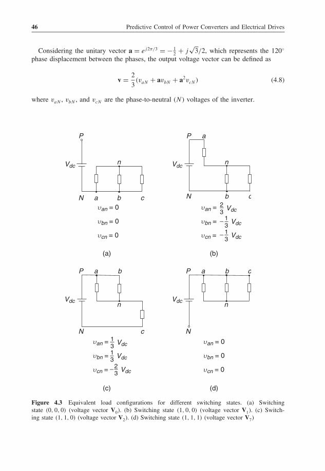
46 Predictive Control of Power Converters and Electrical Drives
Considering the unitary vector a = ej2π/3 = − 12 + j
√3/2, which represents the 120◦
phase displacement between the phases, the output voltage vector can be defined as
v = 2
3(vaN + avbN + a2vcN) (4.8)
where vaN , vbN , and vcN are the phase-to-neutral (N) voltages of the inverter.
(a) (b)
(c) (d)
P
n
ba cNuan = 0
ubn = 0
ucn = 0
Vdc
uan = 0
ubn = 0
ucn = 0
P
n
ba c
N
Vdc
P a
n
b c23
N
uan =
ubn =
ucn =
Vdc
Vdc
13
Vdc
13
Vdc
P
n
ba
cN
Vdc
13
uan =
ubn =
ucn =
Vdc
13 Vdc
23 Vdc
−
−
−
Figure 4.3 Equivalent load configurations for different switching states. (a) Switchingstate (0, 0, 0) (voltage vector V0). (b) Switching state (1, 0, 0) (voltage vector V1). (c) Switch-ing state (1, 1, 0) (voltage vector V2). (d) Switching state (1, 1, 1) (voltage vector V7)
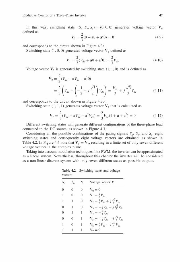
Predictive Control of a Three-Phase Inverter 47
In this way, switching state (Sa, Sb, Sc) = (0, 0, 0) generates voltage vector V0defined as
V0 = 2
3(0 + a0 + a20) = 0 (4.9)
and corresponds to the circuit shown in Figure 4.3a.Switching state (1, 0, 0) generates voltage vector V1 defined as
V1 = 2
3(Vdc + a0 + a20) = 2
3Vdc (4.10)
Voltage vector V2 is generated by switching state (1, 1, 0) and is defined as
V2 = 2
3(Vdc + aVdc + a20)
= 2
3
(Vdc +
(−1
2+ j
√3
2
)Vdc
)= Vdc
3+ j
√3
3Vdc (4.11)
and corresponds to the circuit shown in Figure 4.3b.Switching state (1, 1, 1) generates voltage vector V7 that is calculated as
V7 = 2
3(Vdc + aVdc + a2Vdc) = 2
3Vdc(1 + a + a2) = 0 (4.12)
Different switching states will generate different configurations of the three-phase loadconnected to the DC source, as shown in Figure 4.3.
Considering all the possible combinations of the gating signals Sa , Sb, and Sc, eightswitching states and consequently eight voltage vectors are obtained, as shown inTable 4.2. In Figure 4.4 note that V0 = V7, resulting in a finite set of only seven differentvoltage vectors in the complex plane.
Taking into account modulation techniques, like PWM, the inverter can be approximatedas a linear system. Nevertheless, throughout this chapter the inverter will be consideredas a non linear discrete system with only seven different states as possible outputs.
Table 4.2 Switching states and voltagevectors
Sa Sb Sc Voltage vector V
0 0 0 V0 = 0
1 0 0 V1 = 23 Vdc
1 1 0 V2 = 13 Vdc + j
√3
3 Vdc
0 1 0 V3 = − 13 Vdc + j
√3
3 Vdc
0 1 1 V4 = − 23 Vdc
0 0 1 V5 = − 13 Vdc − j
√3
3 Vdc
1 0 1 V6 = 13 Vdc − j
√3
3 Vdc
1 1 1 V7 = 0

48 Predictive Control of Power Converters and Electrical Drives
V7 (1,1,1)
V0 (0,0,0)
V6 (1,0,1)V5 (0,0,1)
V2 (1,1,0)Im
Re
V3 (0,1,0)
V4 (0,1,1) V1 (1,0,0)
Figure 4.4 Voltage vectors in the complex plane
We should note that a more complex model of the converter model could be usedfor higher switching frequencies. It might include modeling dead time, IGBT saturationvoltage, and diode forward voltage drop, for example. However, in this book, emphasishas been put on simplicity, so a simple model of the inverter will be used.
4.5 Load Model
Taking into account the definitions of variables from the circuit shown in Figure 4.2, theequations for load current dynamics for each phase can be written as
vaN = Ldia
dt+ Ria + ea + vnN (4.13)
vbN = Ldib
dt+ Rib + eb + vnN (4.14)
vcN = Ldic
dt+ Ric + ec + vnN (4.15)
where R is the load resistance and L the load inductance.By substituting (4.13)–(4.15) into (4.8) a vector equation for the load current dynamics
can be obtained:
v = Ld
dt
(2
3(ia + aib + a2ic)
)+ R
(2
3(ia + aib + a2ic)
)
+ 2
3(ea + aeb + a2ec) + 2
3(vnN + avnN + a2vnN) (4.16)
Considering the space vector definition for the inverter voltage given by (4.8), and thefollowing definitions for load current and back-emf space vectors
i = 2
3(ia + aib + a2ic) (4.17)
e = 2
3(ea + aeb + a2ec) (4.18)
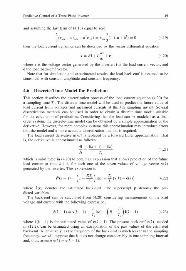
Predictive Control of a Three-Phase Inverter 49
and assuming the last term of (4.16) equal to zero
2
3(vnN + avnN + a2vnN) = vnN
2
3(1 + a + a2) = 0 (4.19)
then the load current dynamics can be described by the vector differential equation
v = Ri + Ldidt
+ e (4.20)
where v is the voltage vector generated by the inverter, i is the load current vector, ande the load back-emf vector.
Note that for simulation and experimental results, the load back-emf is assumed to besinusoidal with constant amplitude and constant frequency.
4.6 Discrete-Time Model for Prediction
This section describes the discretization process of the load current equation (4.20) fora sampling time Ts . The discrete-time model will be used to predict the future value ofload current from voltages and measured currents at the kth sampling instant. Severaldiscretization methods can be used in order to obtain a discrete-time model suitablefor the calculation of predictions. Considering that the load can be modeled as a first-order system, the discrete-time model can be obtained by a simple approximation of thederivative. However, for more complex systems this approximation may introduce errorsinto the model and a more accurate discretization method is required.
The load current derivative di/dt is replaced by a forward Euler approximation. Thatis, the derivative is approximated as follows:
didt
≈ i(k + 1) − i(k)
Ts
(4.21)
which is substituted in (4.20) to obtain an expression that allows prediction of the futureload current at time k + 1, for each one of the seven values of voltage vector v(k)
generated by the inverter. This expression is
ip(k + 1) =(
1 − RTs
L
)i(k) + Ts
L
(v(k) − e(k)
)(4.22)
where e(k) denotes the estimated back-emf. The superscript p denotes the pre-dicted variables.
The back-emf can be calculated from (4.20) considering measurements of the loadvoltage and current with the following expression;
e(k − 1) = v(k − 1) − L
Ts
i(k) −(
R − L
Ts
)i(k − 1) (4.23)
where e(k − 1) is the estimated value of e(k − 1). The present back-emf e(k), neededin (12.2), can be estimated using an extrapolation of the past values of the estimatedback-emf. Alternatively, as the frequency of the back-emf is much less than the samplingfrequency, we will suppose that it does not change considerably in one sampling intervaland, thus, assume e(k) = e(k − 1).
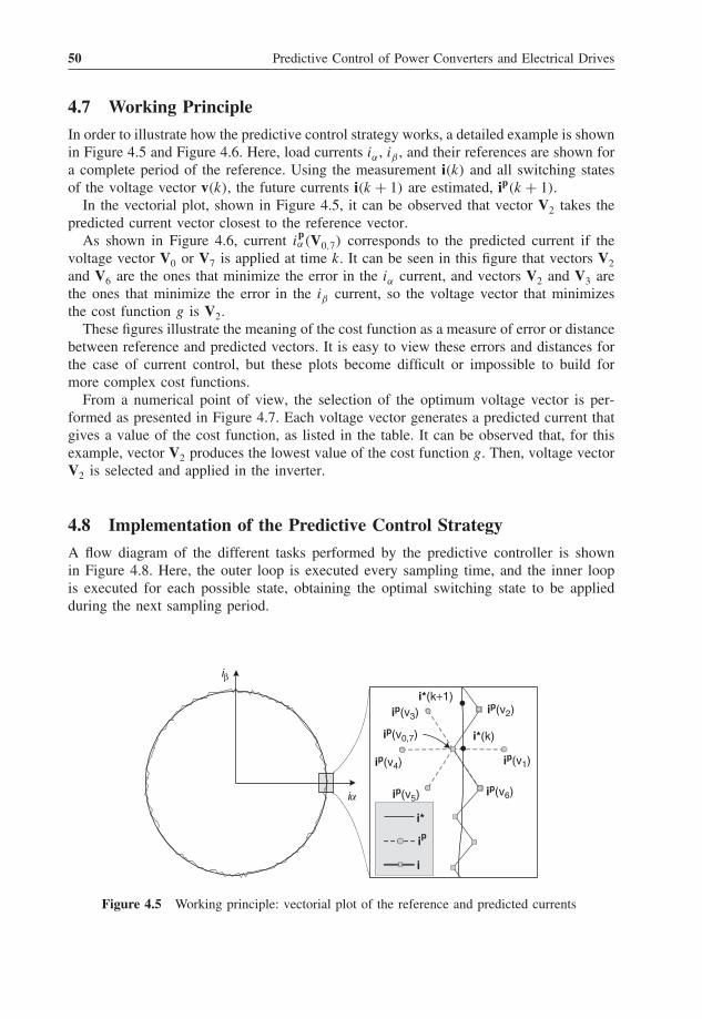
50 Predictive Control of Power Converters and Electrical Drives
4.7 Working Principle
In order to illustrate how the predictive control strategy works, a detailed example is shownin Figure 4.5 and Figure 4.6. Here, load currents iα , iβ , and their references are shown fora complete period of the reference. Using the measurement i(k) and all switching statesof the voltage vector v(k), the future currents i(k + 1) are estimated, ip(k + 1).
In the vectorial plot, shown in Figure 4.5, it can be observed that vector V2 takes thepredicted current vector closest to the reference vector.
As shown in Figure 4.6, current ipα(V0,7) corresponds to the predicted current if the
voltage vector V0 or V7 is applied at time k. It can be seen in this figure that vectors V2and V6 are the ones that minimize the error in the iα current, and vectors V2 and V3 arethe ones that minimize the error in the iβ current, so the voltage vector that minimizesthe cost function g is V2.
These figures illustrate the meaning of the cost function as a measure of error or distancebetween reference and predicted vectors. It is easy to view these errors and distances forthe case of current control, but these plots become difficult or impossible to build formore complex cost functions.
From a numerical point of view, the selection of the optimum voltage vector is per-formed as presented in Figure 4.7. Each voltage vector generates a predicted current thatgives a value of the cost function, as listed in the table. It can be observed that, for thisexample, vector V2 produces the lowest value of the cost function g. Then, voltage vectorV2 is selected and applied in the inverter.
4.8 Implementation of the Predictive Control Strategy
A flow diagram of the different tasks performed by the predictive controller is shownin Figure 4.8. Here, the outer loop is executed every sampling time, and the inner loopis executed for each possible state, obtaining the optimal switching state to be appliedduring the next sampling period.
ip(v1)
ip(v6)
ip(v4)
ip(v3) ip(v2)
i*
i
ip(v5)
iβ
ip(v0,7)
ia
ip
i*(k)
i*(k+1)
Figure 4.5 Working principle: vectorial plot of the reference and predicted currents

Predictive Control of a Three-Phase Inverter 51
tk tk +1
Ts
t
iα(v1)
iα(v2,6)
iα(v4)
iα(v3,5)
iα(v0,7)
iα
iα*
iα
iα
p
p
p
p
p
p
Ts
t
ib(v2,3)
ib(v5,6)
ib(v0,1,4,7)
tk tk +1
ib*
ib
ib
p
p
p
ibp
Figure 4.6 Working principle: reference and predicted currents
The timing of the different tasks is shown in Figure 4.9, and, as illustrated here, themost time-consuming task is the prediction and selection of the optimal switching state.This is due to the calculation of the load model and cost function, which is executedseven times, once for each different voltage vector.
The predictive current control strategy is implemented for simulation in MATLAB asa S-Function, containing the following code:

52 Predictive Control of Power Converters and Electrical Drives
ek = v(xop_1) - L/Ts*ik - (R-L/Ts)*ik_1;g_opt = inf;for i=1:7
ik1 = (1-R*Ts/L)*ik + Ts/L*(v(i)-ek);g = abs(real(ik_ref-ik1)) + abs(imag(ik_ref-ik1));if (g<g_opt)
g_opt = g;x_opt = i;
endendxop_1=xop;xop=x_opt;
where ik= i(k), ik1= i(k + 1), ik_1= i(k − 1), and ek= e(k). The optimal voltagevector that minimize the error is v(xop).
When the predictive control is implemented experimentally, the same code is rewrittenin C language with alpha and beta currents calculated separately.
Results using the control algorithm implemented in MATLAB/Simulink are shownnext, considering (4.22) for load current prediction and (4.23) for back-emf estimation.The system parameters Vdc = 520 V, L = 10 mH, R = 10 �, and e = 100 Vpeak have beenconsidered for simulations.
Current and voltage in one phase of the load are shown in Figure 4.10 for a samplingtime Ts = 100 μs. There is no steady state error in the current but there is a noticeable
V3 V2
V4 V1
V0,V7
V5
g3 g2
g1g4
g0,7
Im
Re
g5 g6V6
Voltage vector Cost functionV0,V7 g0,7 = 0.60
V1 g1 = 0.82
V2 g2 = 0.24 ←optimum
V3 g3 = 0.42
V4 g4 = 0.96
V5 g5 = 1.24
V6 g6 = 1.19
Figure 4.7 Working principle: values of the cost function for each voltage vector
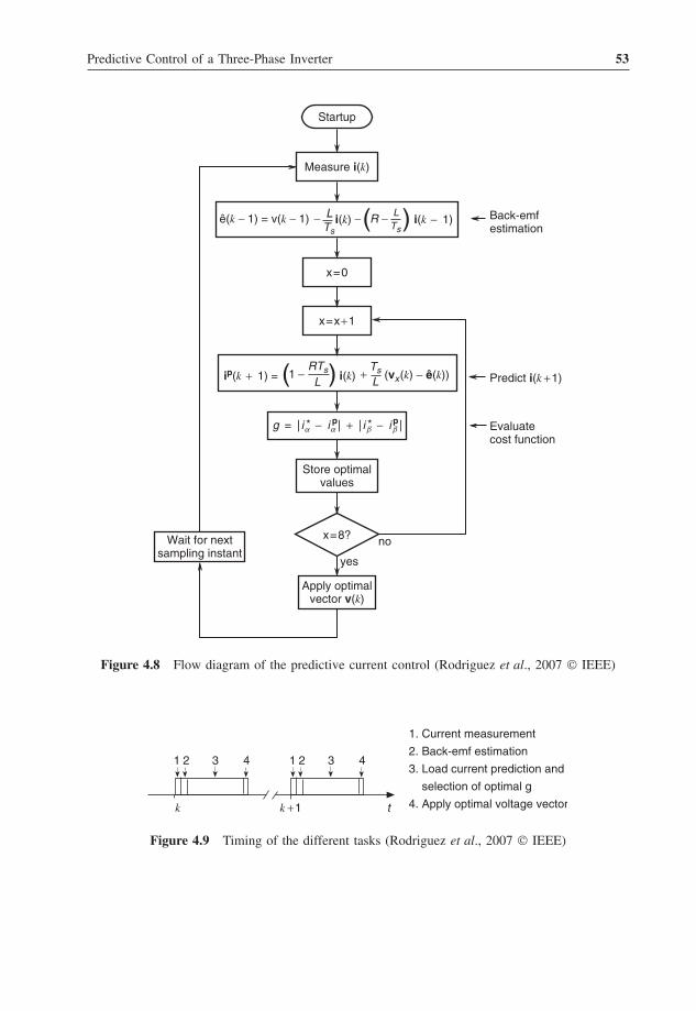
Predictive Control of a Three-Phase Inverter 53
Startup
Back-emfestimation
Predict i(k +1)
Evaluatecost function
Measure i(k)
x=0
x=x+1
Store optimalvalues
x=8?
Apply optimalvector v(k)
Wait for nextsampling instant
no
yes
i(k) i(k − 1)ê(k − 1) = v(k − 1) − R −−LTs
LTs
( )
ip(k + 1) = i(k) (vx(k) − ê(k))+LTs1 −
RTs
L( )
g = | ia − ia | + | ib − ib |* p * p
Figure 4.8 Flow diagram of the predictive current control (Rodriguez et al., 2007 © IEEE)
1
k k +1 t
2 3 4 1 2 3 4
1. Current measurement
2. Back-emf estimation
3. Load current prediction and
selection of optimal g
4. Apply optimal voltage vector
Figure 4.9 Timing of the different tasks (Rodriguez et al., 2007 © IEEE)
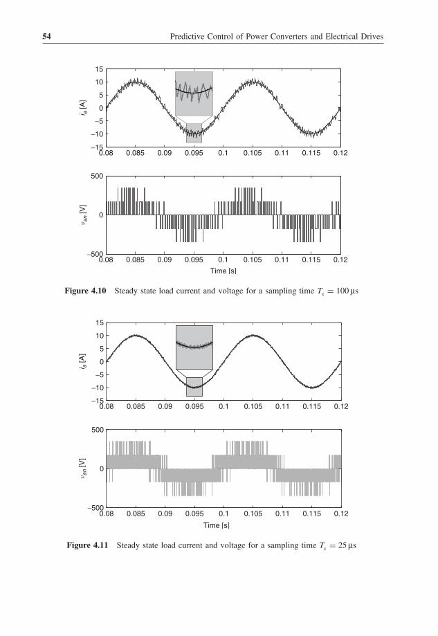
54 Predictive Control of Power Converters and Electrical Drives
0.08 0.085 0.09 0.095 0.1 0.105 0.11 0.115 0.12−15
−10
−5
0
5
10
15
i a [A
]
0.08 0.085 0.09 0.095 0.1 0.105 0.11 0.115 0.12−500
0
500
nan
[V]
Time [s]
Figure 4.10 Steady state load current and voltage for a sampling time Ts = 100 μs
0.08 0.085 0.09 0.095 0.1 0.105 0.11 0.115 0.12−15
−10
−5
0
5
10
15
i a [A
]
−500
0
500
nan
[V]
Time [s]
0.08 0.085 0.09 0.095 0.1 0.105 0.11 0.115 0.12
Figure 4.11 Steady state load current and voltage for a sampling time Ts = 25 μs

Predictive Control of a Three-Phase Inverter 55
Time [s]
100
50
0
−50
−100
0.08 0.085 0.09 0.095 0.1 0.105 0.11 0.115 0.12
back
- e
mf [
V]
0.08 0.085 0.09 0.095 0.1 0.105 0.11 0.115 0.12
100
50
0
−50
−100estim
ated
bac
k -
emf [
V]
Figure 4.12 Real and estimated back-emf
ripple. This ripple is reduced considerably when a smaller sampling time is used, as shownin Figure 4.11 for a sampling time Ts = 25 μs. However, by reducing the sampling time,the switching frequency is increased as can be seen by comparing the load voltages inFigure 4.10 and Figure 4.11.
Real and estimated back-emf are shown in Figure 4.12. Back-emf is estimated using(4.23) with a sampling time Ts = 25 μs.
The response of the system to a step in the amplitude of the reference current vector i∗
is shown in Figure 4.13. It can be observed that the load currents follow their referenceswith fast dynamics. It is also shown in this figure how the load voltage changes duringthe reference current step.
The predictive current control strategy was implemented with the experimental setupdescribed in Figure 4.14. A Danfoss VLT5008 5.5 kW three-phase inverter with an RLload is used. The DC link is fed by a three-phase diode bridge rectifier. The inverter iscontrolled externally through an interface and protection card (IPC). A TMS320C6713floating-point DSP was used for the control. The gate drive signals for each inverter legare sent from the DSP to the IPC through fiber optic cables. Current measurements of twophases are sent back from the inverter to the DSP through coaxial cables. A FPGA-baseddaughter card handles the analog to digital conversion, digital to analog conversion, andthe digital outputs for the DSP. The execution time for the implemented current controlalgorithm was about 7 μs. The parameters of the experimental setup are Vdc = 520 V,L = 10 mH, R = 10 �, e = 0 Vpeak , and Ts = 25 μs.
The behavior of the load currents and the voltage in one phase at steady state operationis shown in Figure 4.15. The amplitude of the reference current was set to 10 A with afrequency of 50 Hz. Currents are sinusoidal with low harmonic distortion.

56 Predictive Control of Power Converters and Electrical Drives
Time [s]
0.02 0.025 0.03 0.035 0.04 0.045 0.05 0.055 0.06−400
−200
0
200
400
nan
[V]
0.02 0.025 0.03 0.035 0.04 0.045 0.05 0.055 0.06−15
−10
−5
0
5
10
15
i α,i
β [A
]i α
, iβ
[A]
iα iβ
0.0325 0.0335 0.0355 0.0365 0.0375−11
−8
−5
−2
1
4
0.0345
iβ
iα
Figure 4.13 Load currents for a step in the amplitude of the reference current vector i∗, withsampling time Ts = 25 μs
Results for a step change in the amplitude of the reference i∗α from 5 to 10 A areshown in Figure 4.16. The amplitude of the reference current i∗β is kept at 10 A. It canbe observed that the load current iα reaches its reference with very fast dynamics whileiβ is not affected by this step change. This result shows that the currents are decoupledin the predictive current control scheme. The load voltage van for the same test is shownin Figure 4.17. It can be seen that during the step change of current iα the load voltageis kept at its maximum value until the reference current is achieved.
The behavior of the load currents and load voltage for a step in the amplitude of thereference current vector is shown in Figure 4.18. The amplitude of the reference currentchanges from 10 to 5 A and later from 5 to 10 A for all phases. The reference current i∗ais also shown in the figure. It can be seen that the amplitude of the load currents changesvery quickly following the change of the reference. It is also shown in the figure how theload voltage van changes during this test.
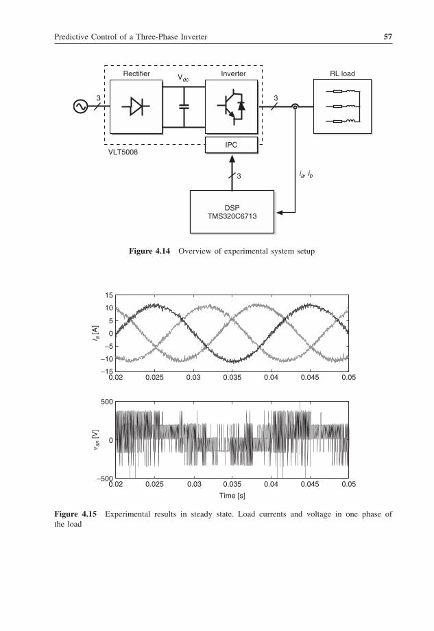
Predictive Control of a Three-Phase Inverter 57
VLT5008
Rectifier InverterVdc
ia, ib3
33
RL load
IPC
DSPTMS320C6713
Figure 4.14 Overview of experimental system setup
−500
0
500
nan
[V]
Time [s]
0.02 0.025 0.03 0.035 0.04 0.045 0.05−15
−10
−5
0
5
10
15
i a [A
]
0.02 0.025 0.03 0.035 0.04 0.045 0.05
Figure 4.15 Experimental results in steady state. Load currents and voltage in one phase ofthe load

58 Predictive Control of Power Converters and Electrical Drives
0.02 0.022 0.024 0.026 0.028 0.03 0.032 0.034 0.036 0.038 0.04
0.02 0.022 0.024 0.026 0.028 0.03 0.032 0.034 0.036 0.038 0.04
−15
−10
−5
0
5
10
15
−15
−10
−5
0
5
10
15
i β [A
]
Time [s]
iα*
iα
i α, i
α [A
]*
Figure 4.16 Experimental results for a step in the amplitude of i∗α . Load currents
−15
−10
−5
0
5
10
15
−500
0
500
Time [s]
nan
[V]
iα
iα
*
i α, i
α [A
]*
0.02 0.022 0.024 0.026 0.028 0.03 0.032 0.034 0.036 0.038 0.04
0.02 0.022 0.024 0.026 0.028 0.03 0.032 0.034 0.036 0.038 0.04
Figure 4.17 Experimental results for a step in the amplitude of i∗α . Load current and voltage
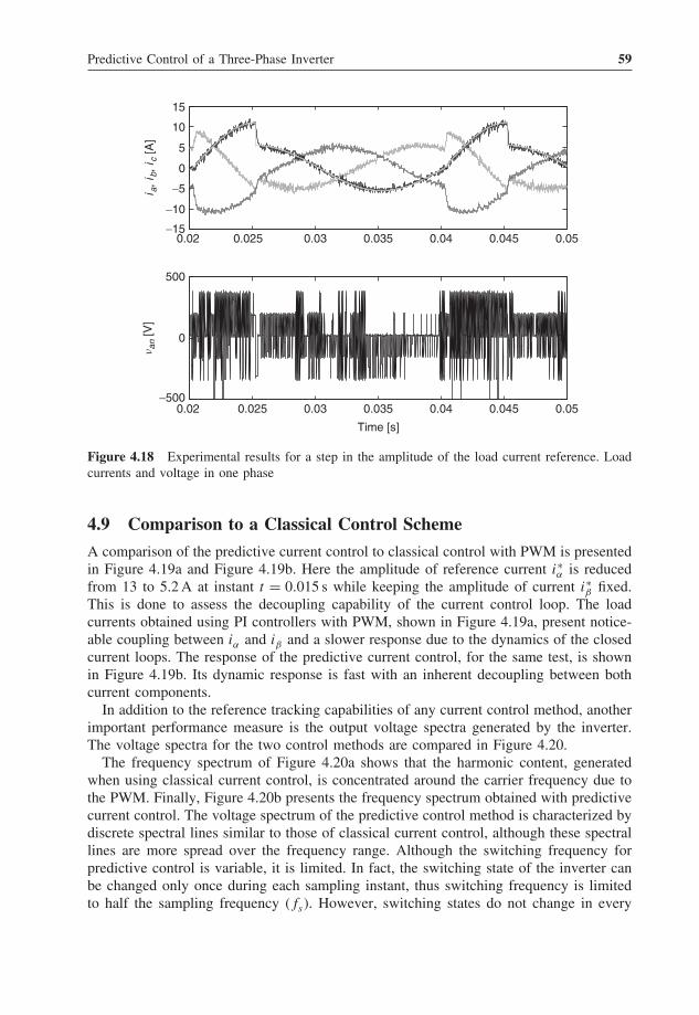
Predictive Control of a Three-Phase Inverter 59
0.02 0.025 0.03 0.035 0.04 0.045 0.05−15
−10
−5
0
5
10
15
i a, i
b, i
c [A
]
0.02 0.025 0.03 0.035 0.04 0.045 0.05−500
0
500
nan
[V]
Time [s]
Figure 4.18 Experimental results for a step in the amplitude of the load current reference. Loadcurrents and voltage in one phase
4.9 Comparison to a Classical Control Scheme
A comparison of the predictive current control to classical control with PWM is presentedin Figure 4.19a and Figure 4.19b. Here the amplitude of reference current i∗α is reducedfrom 13 to 5.2 A at instant t = 0.015 s while keeping the amplitude of current i∗β fixed.This is done to assess the decoupling capability of the current control loop. The loadcurrents obtained using PI controllers with PWM, shown in Figure 4.19a, present notice-able coupling between iα and iβ and a slower response due to the dynamics of the closedcurrent loops. The response of the predictive current control, for the same test, is shownin Figure 4.19b. Its dynamic response is fast with an inherent decoupling between bothcurrent components.
In addition to the reference tracking capabilities of any current control method, anotherimportant performance measure is the output voltage spectra generated by the inverter.The voltage spectra for the two control methods are compared in Figure 4.20.
The frequency spectrum of Figure 4.20a shows that the harmonic content, generatedwhen using classical current control, is concentrated around the carrier frequency due tothe PWM. Finally, Figure 4.20b presents the frequency spectrum obtained with predictivecurrent control. The voltage spectrum of the predictive control method is characterized bydiscrete spectral lines similar to those of classical current control, although these spectrallines are more spread over the frequency range. Although the switching frequency forpredictive control is variable, it is limited. In fact, the switching state of the inverter canbe changed only once during each sampling instant, thus switching frequency is limitedto half the sampling frequency (fs). However, switching states do not change in every
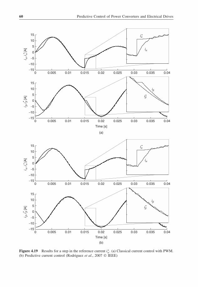
60 Predictive Control of Power Converters and Electrical Drives
0 0.005 0.01 0.015 0.02 0.025 0.03 0.035 0.04
0 0.005 0.01 0.015 0.02 0.025 0.03 0.035 0.04
0 0.005 0.01 0.015 0.02 0.025 0.03 0.035 0.04
0 0.005 0.01 0.015 0.02 0.025 0.03 0.035 0.04
−15
−10
−5
0
5
10
15
−15
−10
−5
0
5
10
15
Time [s]
(a)
(b)
iα
*iα
*iβ
iβ
−15
−10
−5
0
5
10
15
−15
−10
−5
0
5
10
15
Time [s]
*i β
,iβ
[A]
*i α
,iα [A
]*
i β,i
β [A
]*
i α,i
α [A
]
iα
*iα
*iβ
iβ
Figure 4.19 Results for a step in the reference current i∗α . (a) Classical current control with PWM.(b) Predictive current control (Rodriguez et al., 2007 © IEEE)

Predictive Control of a Three-Phase Inverter 61
0 1000 2000 3000 4000 5000
(a)
(b)
6000 7000 8000 9000 100000
10
20
30
40M
agni
tude
[%]
PWMTHDV = 38%
0 1000 2000 3000 4000 5000 6000 7000 8000 9000 100000
10
20
30
40
Frequency [Hz]
PredictiveTHDV = 28.2%
Figure 4.20 Load voltage spectrum
sampling instant, therefore the average switching frequency is always less than fs/2.Results show that the average switching frequency is concentrated between fs/5 andfs/4. Additionally, the switching frequency can be controlled by modification of the costfunction as will be shown in the next application example.
An assessment of the operating principles between a classical current control schemeand a predictive current control scheme is presented in Table 4.3. Although the predictivecontrol scheme is based on more advanced control theory, the resulting control strategyis no more complex than a classical scheme based on PI controllers and SVM. Bothcontrol schemes need a model of the inverter and the voltage vectors that it generates.In the classical scheme, knowledge of the voltage vectors is used for implementation ofthe modulator. For predictive control, these voltage vectors are the finite set of possibleactuations. In order to adjust the PI controllers, a linear model of the load is needed. Thepredictive controller will calculate predictions for each voltage vector using a discrete-timemodel of the load, which does not need to be linear. The performance of the PI controllersdepends on the appropriate adjustment of their parameters kp and ki . In the predictivecontrol scheme there are no parameters to adjust, but a cost function must be defined,which in the case of current control is very simple. The space vector modulator mustbe implemented by considering the calculation of the application times of the selectedvoltage vectors as explained in Section 2.1.2. This stage is not needed in the predictivecontrol scheme as the switching states are generated directly by the controller.

Tabl
e4.
3A
sses
smen
tof
oper
atin
gpr
inci
ples
Cur
rent
Con
trol
with
SVM
Pred
ictiv
eC
ontr
ol
+ −
3M 3φ
Spa
ceV
ecto
rM
odul
atio
n(S
VM
)
i*
i
vv*
Sa
Sb
Sc
Sa
Sb
Sc
Pre
dict
ive
mod
el
i*(k
)M
inim
izat
ion
of c
ost
func
tion
7
3φ M3
Inve
rter
i(k)
ip(k
+1)
1.SV
Mus
esse
ven
volta
geve
ctor
sfo
rm
odul
atio
n1.
MPC
uses
seve
nvo
ltage
vect
ors
for
pred
ictio
n
2.L
inea
rm
odel
v=
Ri+
Ld
idt
+e
2.L
oad
mod
elfo
rpr
edic
tion
(can
beno
nlin
ear)
:
ip(k
+1)
=( 1
−R
Ts
L
) i(k)+
Ts L
( v(k)−
e(k))
3.C
ontr
olle
rad
just
men
t:
v∗
=k
p(i
∗−
i)+
ki
∫ (i∗−
i)dt
3.C
ost
tofu
nctio
n:ev
alua
ted
for
each
volta
geve
ctor
:
g=
|i∗ α−
ip α|+
|i∗ β−
ip β|
with
sele
ctio
nof
gop
timal
.
4.Sp
ace
vect
orm
odul
atio
n(S
VM
)
v∗=
1 T(v
at a
+v b
t b+
v 0t 0
)
T=
t a+
t b+
t 0

Predictive Control of a Three-Phase Inverter 63
4.10 Summary
This chapter presents one of the simplest predictive control schemes: current control ina three-phase inverter. This example allows us to introduce this control method in thefield of power electronics. A simple model of the converter and the load is presented.Then the predictive current control method is explained in detail. Results are presentedand compared to a classical current control scheme.
References[1] J. Holtz, “Pulsewidth modulation electronic power conversion,” Proceedings of the IEEE , vol. 82, no. 8,
pp. 1194–1214, August 1994.[2] M. P. Kazmierkowski, R. Krishnan, and F. Blaabjerg, Control in power electronics . Academic Press, 2002.[3] N. Mohan, T. M. Undeland, and W. P. Robbins, Power electronics , 3rd ed. John Wiley & Sons, Inc., 2003.[4] J. Rodrıguez, J. Pontt, C. Silva et al. “Predictive current control of a voltage source inverter,” IEEE
Transactions on Industrial Electronics , vol. 54, no. 1, pp. 495–503, February 2007.