comparative analysis of principal ... - daniel s. caetano

Syst. Biol. 64(4):677–689, 2015© The Author(s) 2015. Published by Oxford University Press, on behalf of the Society of Systematic Biologists. All rights reserved.For Permissions, please email: [email protected]:10.1093/sysbio/syv019Advance Access publication April 3, 2015

Comparative Analysis of Principal Components Can be Misleading

JOSEF C. UYEDA∗, DANIEL S. CAETANO, AND MATTHEW W. PENNELL

Department of Biological Sciences, Institute for Bioinformatics and Evolutionary Studies, University of Idaho, Moscow, ID 83844, USA.∗Correspondence to be sent to: Department of Biological Sciences, Institute for Bioinformatics and Evolutionary Studies, University of Idaho,

Moscow, ID 83844, USA; E-mail: [email protected]

Received 21 July 2014; reviews returned 28 October 2014; accepted 30 March 2015Associate Editor: Tanja Stadler

Abstract.—Most existing methods for modeling trait evolution are univariate, although researchers are often interested ininvestigating evolutionary patterns and processes across multiple traits. Principal components analysis (PCA) is commonlyused to reduce the dimensionality of multivariate data so that univariate trait models can be fit to individual principalcomponents. The problem with using standard PCA on phylogenetically structured data has been previously pointed outyet it continues to be widely used in the literature. Here we demonstrate precisely how using standard PCA can misleadinferences: The first few principal components of traits evolved under constant-rate multivariate Brownian motion willappear to have evolved via an “early burst” process. A phylogenetic PCA (pPCA) has been proprosed to alleviate theseissues. However, when the true model of trait evolution deviates from the model assumed in the calculation of the pPCAaxes, we find that the use of pPCA suffers from similar artifacts as standard PCA. We show that data sets with high effectivedimensionality are particularly likely to lead to erroneous inferences. Ultimately, all of the problems we report stem fromthe same underlying issue—by considering only the first few principal components as univariate traits, we are effectivelyexamining a biased sample of a multivariate pattern. These results highlight the need for truly multivariate phylogeneticcomparative methods. As these methods are still being developed, we discuss potential alternative strategies for usingand interpreting models fit to univariate axes of multivariate data. [Brownian motion; early burst; multivariate evolution;Ornstein–Uhlenbeck; phylogenetic comparative methods; principal components analysis; quantitative genetics]

Quantitative geneticists long ago recognized the valueof studying evolution in a multivariate framework(Pearson 1903). Due to linkage, pleiotropy, correlatedselection, and mutational covariance, the evolutionaryresponse in any phenotypic trait can only be properlyunderstood in the context of other traits (Lande 1979;Lynch and Walsh 1998). This is of course also wellappreciated by comparative biologists. However, unlikein quantitative genetics, most of the statistical andconceptual tools for analyzing phylogenetic comparativedata (reviewed in Pennell and Harmon 2013) model asingle trait (but see, Revell and Harmon 2008; Revelland Harrison 2008; Hohenlohe and Arnold 2008; Revelland Collar 2009; Schmitz and Motani 2011; Bartoszeket al. 2012; Adams 2014a,b, for exceptions). Indeed, evenclassical approaches for testing for correlated evolutionbetween two traits (e.g., Felsenstein 1985; Grafen 1989)are not actually multivariate as each trait is assumedto have evolved under a process that is independent ofthe state of the other (Hansen and Orzack 2005). As aresult of these limitations, researchers with multivariatedata are often faced with a choice: analyze each trait asif they are independent, or else decompose the data setinto statistically independent sets of traits, such that eachset can be analyzed with the univariate methods.

Principal components analysis (PCA) is the mostcommon method for reducing the dimensionalityof the data set prior to analyzing the data usingphylogenetic comparative methods. PCA is a projectionof multivariate data onto a new coordinate system.

The first PC axis is the eigenvector in the directionof greatest variance, the second PC axis, the secondgreatest variance, and so on. While PCA is simplyanother way of representing a data set, whetheror not one can draw meaningful inferences fromthe PC axes will depend on both the question andthe structure of the data. Evolution introduces aparticular kind of structure into comparative data: asa result of shared common ancestry, close relativesare likely to share many traits and trait combinations.Performing comparative analyses without consideringthe species’ evolutionary relationships is anathemato most evolutionary biologists, but the influence ofphylogeny on data transformations is less understood(Revell 2009; Polly et al. 2013).

Standard PCA continues to be regularly used incomparative biology. Researchers fit models to PCscores computed from a variety of trait types includinggeometric morphometric landmarks (e.g., Dornburget al. 2011; Hunt 2013), measurements of multiplemorphological traits (e.g., Harmon et al. 2010; Weir andMursleen 2013; Pienaar et al. 2013; Price et al. 2014), andclimatic variables (e.g., Kozak and Wiens 2010; Schnitzleret al. 2012). The papers we have cited here are simplyexamples selected from a substantial number wherestandard PCA was used.

The most common approach for incorporating the nonindependence of species is to assume a phylogeneticmodel for the evolution of measured traits and use theexpected covariance in the calculation of the PC axes and

677

at Universidade de SÃ

¯Â¿Â

½o Paulo on January 9, 2016

http://sysbio.oxfordjournals.org/D

ownloaded from

http://sysbio.oxfordjournals.org/

678 SYSTEMATIC BIOLOGY VOL. 64

scores (phylogenetic principal components analysis, orpPCA; Revell 2009). Revell’s method, explained in detailbelow, assumes that the measured traits have evolvedunder a multivariate Brownian motion (BM) process oftrait evolution. Revell (2009) demonstrated that standardPCA produces eigenvalues and eigenvectors that are notphylogenetically independent.

In this article, we first extend the argument of Revell(2009) and demonstrate how performing phylogeneticcomparative analyses on standard PC axes can bepositively misleading. This point has been madein other fields that deal with autocorrelated data,such as population genetics (Novembre and Stephens2008), ecology (Podani and Miklós 2002), climatology(Richman 1986), and paleobiology (Bookstein 2012).However, the connection between these previous resultsand phylogenetic comparative data has not been widelyappreciated and standard PCs continue to be regularlyused in the field. We hope our article helps change thispractice.

Second, as stated above, Revell (2009) assumed thatthe measured traits had evolved under a multivariateBM process. As the pPC scores are not phylogeneticallyindependent (Revell 2009; also see discussion in Pollyet al. 2013), one must use comparative methods toanalyze them, which will in turn require selectingan evolutionary model for the scores. The choice ofmodel for the traits and the pPC scores are separatesteps in the analysis (Revell 2009). Researchers mustassume a model for the evolution of the traits in orderto obtain the pPC scores and then perform model-based inference on these scores. This introduces somecircularity into the analysis: it seems likely that the choiceof a model for the evolution of the traits will influence theapparent macroevolutionary dynamics of the resultingpPC scores. To our knowledge this effect has not beenpreviously explored. Here we analyze simulated datato investigate whether assuming a BM model for thetraits introduces systematic biases in the pPC scoreswhen the generating model is different. We then analyzetwo empirical comparative data sets to understand theimplications of these results for the types of data thatresearchers actually have; the traits in these data setshave certainly not evolved by a strict BM process.

Last, we consider the interpretation of evolutionarymodels fit to pPC axes and discuss the advantages anddisadvantages of using pPCA compared to alternativeapproaches for studying multivariate evolution in aphylogenetic comparative framework. We argue that thestatistical benefits of using pPC axes come at a substantialconceptual cost and that alternative techniques are likelyto be much more informative for addressing manyevolutionary questions.

METHODS

Overview of pPCABefore describing our analyses, we briefly review

standard and phylogenetic PCA and highlight the

differences between the two (see Polly et al. 2013, for amore detailed treatment). In conventional PCA, a m×mcovariance matrix R is computed from a matrix of traitvalues X for the n species and m traits

R= (n−1)−1(X−1μᵀ)ᵀ(X−1μᵀ) (1)

where μ is a vector containing the means of all m traitsand 1 is a column vector of ones. We note that in manyapplications X may not represent the raw trait values. Ingeometric morphometrics, for example, size, translation,and rotation will often be removed from X prior tocomputing R (Rohlf and Slice 1990; Bookstein 1997). Thescores S, the trait values of the species along the PC axes,are computed as

S= (X−1μᵀ)V (2)

where the columns of V are the eigenvectors of R.Phylogenetic PCA differs from this procedure in two

important ways (Revell 2009; Polly et al. 2013): Firstthe covariance matrix is weighted by the inverse of theexpected covariance of trait values between taxa undera given model �. Under a BM model of trait evolution,� is simply proportional to the matrix representationof the phylogenetic tree C, such that �i,j is the sharedpath length between lineages i and j (Rohlf 2001). Sinceonly relative branch lengths matter under a multivariateBM process, we can simply set �=C without loss ofgenerality, though we note that the absolute magnitudeof the eigenvalues will depend on the scale of thebranch lengths. Second, the space is centered on the“phylogenetic means” a of the traits rather than theirarithmetic means, which can be computed followingRevell and Harmon (2008):

a=[(1ᵀ�−11)−11ᵀ�−1X]ᵀ (3)

In pPCA, Equation 1 is therefore modified as

R= (n−1)−1(X−1aᵀ)ᵀ�−1(X−1aᵀ) (4)

Similarly, S can be calculated for pPCA using Equation 2but substituting the phylogenetic means for thearithmetic means

S= (X−1aᵀ)V (5)

where again, V is a matrix containing the eigenvectorsof R, in this case obtained from Equation 4.

The effect of weighting the covariance and centeringthe space using phylogeny has an important statisticalconsequence (Revell 2009; Polly et al. 2013). In PCA,each PC score is independent of all other scores fromthe same PC axis and from scores on other axes. Dueto the phylogenetic structure of the data, this propertyof independence does not hold when using pPCA.Therefore it is necessary to analyze pPC scores usingphylogenetic comparative methods, just as one wouldfor any other trait (Revell 2009).


¯Â¿Â



ownloaded from


2015 POINTS OF VIEW 679

Effect of PCA on Model Selection under Multivariate BMWe simulated 100 replicate data sets under

multivariate BM to evaluate the effect of usingstandard versus phylogenetic PCA to infer the modeof evolution. For each data set, we used TreeSim(Stadler 2011) to simulate a phylogeny of 50 terminaltaxa under a pure-birth process and scaled each tree tounit height. We then simulated a 20-trait data set undermultivariate BM. For each simulation, we generated apositive definite covariance matrix for R, by drawingeigenvalues from an exponential distribution witha rate �=1/100 and randomly oriented orthogonaleigenvectors to reflect the heterogeneity and correlationstructure typical of evolutionary rate matrices (Mezeyand Houle 2005; Griswold et al. 2007). We then usedthis matrix to generate a covariance matrix for the tipstates X∼N (0,R⊗C) where ⊗ denotes the Kroneckerproduct. For each of the 100 simulated data sets, wecomputed PC scores using both standard methods andpPCA (using the phytools package; Revell 2012).We used phylolm (Ho and Ané 2014) to fit models oftrait evolution to the original data and to all PC scoresobtained by both methods. Following Harmon et al.(2010), we considered three models of trait evolution:1) BM; 2) Ornstein–Uhlenbeck with a fixed root (OU:Hansen 1997); and 3) Early-Burst (EB: Blomberg et al.2003; Harmon et al. 2010). We then calculated theAkaike Information Criterion weights (AICw) for eachmodel/transformation/trait combination.

To explore the effect of trait correlation on inference,we conducted an additional set of simulations whereR was varied from the above simulations to result inmore or less correlated sets of phenotypic traits. Wedrew eigenvalues m from an exponential distributionand scaled these so that the leading eigenvalue m1 wasequal to 1. We then exponentiated this vector across asequence of exponents ranging for �1 to �1; this gaveus a series of covariance matrices ranging from highlycorrelated (m1 =1;m2,...,m20 ≈0) to nearly independent(m≈1), respectively. We chose the series of exponents toobtain a regular sequence of m1/

∑20i=1mi from 0.05 to 1.

For each set of eigenvalues, we simulated 25 data setsand estimated the slope of the relationship between theabsolute size of phylogenetically independent contrasts(Felsenstein 1985) and the height of the node at whichthey were calculated (the “node height test”; Purvis andRambaut 1995). Under OU models, this relationship isexpected to be positive, whereas under EB models thisrelationship is negative. BM models are expected not toshow correlation between contrasts and height of thenodes.

Effect of Using PCA When Traits are Not BrownianWe then simulated data sets under alternative models

of trait evolution. First, we also simulated traits under acorrelated multivariate OU model using the mvSLOUCHpackage (Bartoszek et al. 2012). Combined with thecorrelated BM simulations above, we used correlated OU

simulations to explore the effect of PCA and pPCA onmodel inference under reasonably biologically realisticconditions. We simulated 20 correlated traits for 50 taxatrees using a positive definite covariance matrix forthe diffusion matrix by drawing eigenvalues from anexponential distribution with a rate �=1 and randomlyoriented orthogonal eigenvectors. The �-matrix was seta diagonal matrix with a constant value of 2 for each traitsuch that the phylogenetic half-life log(2)/� (Hansenet al. 2008) was approximately equal to 0.35 of the totaltree depth. The root state for each simulation was set atthe multivariate phenotypic optimum. We then fit BM,OU, and EB models to the original data, PC scores andpPC scores for each simulated data set and estimatedparameters and AICw.

Second, we simulated an additional set of data setswith uncorrelated traits and equal evolutionary rates.These simplified data sets allowed us to generatecomparable data under all three generating models (BM,OU, and EB) and isolate how misspecifying the modelof trait evolution can impact the distribution of PC andpPC scores. As before, for each model we simulated20 traits on 50 taxa trees. For the BM simulations,we set �2 =1 for all 20 traits. For OU, we set �2 =1and �=2. For EB, we again set �2 =1 and set r, theexponential rate of deceleration, to be log(0.02). Asabove, we estimated parameters and AICw for eachmodel fit to original data, PC scores and pPC scores.In addition, we applied two common diagnostic testsfor deviation from BM-like evolution to all trait/PCaxes. First, we calculated the slope of the node heighttest as described in the preceding section. Second, wecharacterized the disparity through time (Harmon et al.2003) using the geiger package (Pennell et al. 2014a).

Finally, we examined the scenario in which a setof traits each follow a model of evolution withunique evolutionary parameters. In particular, weuse the accelerating–decelerating (ACDC) model ofBlomberg et al. (2003) to generate independent traitdata sets. This model is a general case of the EBmodel which allows both accelerating or deceleratingrates of phenotypic evolution. Accelerating rates ofevolution result in identical likelihoods as the OU model(assuming the root state is at the optimal trait valueand the tree is ultrametric), and thus are equivalentfor our purposes (we provide a proof for this claimin the Supplementary Material available on Dryad athttp://dx.doi.org/10.5061/dryad.70c34). We simulated100 data sets with 50 taxa and 20 traits. Trees weregenerated as in previous simulations. Each trait wassimulated along the phylogeny with an exponentialrate of change r drawn from a normal distributionwith mean 0 and standard deviation of 5. Values of rabove 0 correspond to accelerating evolutionary rates,whereas those below 0 correspond to decelerating,or EB models of evolution. For each data set, weconducted both standard and phylogenetic PCA inwhich the traits are standardized to unit variance (i.e.,using correlation matrices, which ensured traits acrossparameter values had equal expected variances). For


¯Â¿Â



ownloaded from

http://dx.doi.org/10.5061/dryad.70c34



each PC or pPC, we regressed the magnitude of the traitloadings against the trait’s ACDC parameter value. Wethen visualized whether there were systematic trendsin the relationship between the ACDC parameter value,and the weight given to a particular trait across PC axes.Such systematic trends would indicate that either PCAor pPCA “sorts” traits into PC axes according to theparticular evolutionary model each trait follows.

Empirical ExamplesWe analyzed two comparative data sets assembled

from the literature, allowing us to investigate the effectsof principal components analyses on realisticallystructured data. First, we analyzed phenotypicevolution across the family Felidae (cats) usingmeasurements from two independent sources—fivecranial measurements from (Slater and Van Valkenburgh2009) and body mass and skull width from (Sakamotoet al. 2010). For the analysis, we used the supertreecompiled by (Nyakatura and Bininda-Emonds 2012).Second, we analyzed 23 morphometric traits in Anolislizards and phylogeny from (Mahler et al. 2010). In bothdata sets, all measurements were linear measurementson the logarithmic scale. We conducted standardand phylogenetic PCA and examined the effect ofeach on model-fitting, the slope of the node heighttest, and the average disparity through time. Allsimulations and analyses were conducting using Rv3.0.2. Scripts to reproduce our results are available athttps://github.com/mwpennell/phyloPCA.

RESULTS

Effect of PCA on Model Selection under Multivariate BMStandard PCA introduces a systematic bias in

the favored model across principal components. Inour simulations where the traits evolved under amultivariate BM model, EB models had systematicallyelevated support as measured by Akaike weightsfor the first few components, for which it generallyexceeded support for the BM model (Fig. 1, leftpanel). Fitting models sequentially across PC axes 1–20revealed a regular pattern of increasing support for BMmodels moving from the first toward the intermediatecomponents, followed by increasing support for OUmodels among later components, which generallyapproached an AICw of 1. This regular pattern acrosstrait axes was not present for either the originaldata sets, or for phylogenetic principal components,which found strong support for the BM model regardlessof which trait was analyzed. As BM is a specialcase of both OU and EB, the likelihoods for themore complex models will converge on that of BMwhen the true model is Brownian. AIC weights formodel i are computed as AICwi =exp[0.5(AICmin −AICi)]/

∑j exp[0.5(AICmin −AICj)] and therefore if the

likelihoods are identical, OU and EB will have a

�AIC=AICmin −AICi =2 (as OU and EB each have onemore parameter than BM). The theoretical maximum forthe AICw of BM is thus 1/(2e−1+ 1) ≈0.576.

Multivariate data sets simulated with highcorrelations (i.e., low effective dimensionality) showedincreased support for BM across PC axes. When theleading eigenvalue explained a large proportion of thevariance, the slope of the node height test convergedtoward 0, indicating no systematic distortion of thecontrasts through time (Fig. 2). However, when theeigenvalues of the rate matrix were more even, standardPCA resulted in a negative slope in the node heighttest among the first few PCs, which in turn provideselevated support for EB models. This pattern is reversedamong higher PC axes, which have positive slopesbetween node height and absolute contrast size, whichprovides elevated support for OU models (Figs. 2and 3).

Effect of Using PCA When Traits are Not BrownianIf the underlying model was either OU or EB rather

than BM, then phylogenetic PCA tend to increasesupport for the true model relative to the originaltrait variables for the first few component axes (Fig. 1,right panel; Figs. S.1 and S.2 available on Dryad athttp://dx.doi.org/10.5061/dryad.70c34). For example,when each of the original trait variables were simulatedunder a correlated or uncorrelated OU process, supportfor the OU model increased for pPC1 relative to theoriginal trait variables. Higher PC axes showed a regularpattern of decreasing support for the OU model, whilethe last few PCs have equivocal support for either aBM or OU model (Fig. 1, right panel Fig. S.1 availableon Dryad at http://dx.doi.org/10.5061/dryad.70c34).Furthermore, parameter estimation was affected byphylogenetic PCA. The � parameter of the correlatedand uncorrelated OU models were estimated to bestronger than the value simulated for individual traitsfor the first few pPC scores and lower for the highercomponents (Figs. S.3 and S.4 available on Dryad athttp://dx.doi.org/10.5061/dryad.70c34).

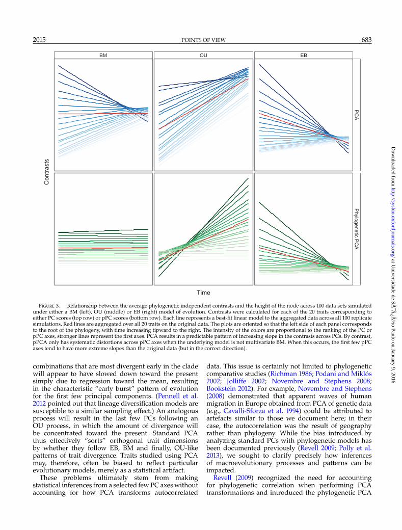
Examining the outcomes of the node height tests(Fig. 3) and the disparity through time analyses(Fig. S.5 available on Dryad at http://dx.doi.org/10.5061/dryad.70c34) for uncorrelated OU, EB and BMmodels helps clarify the results we observed frommodel comparison and parameter estimation. Under OUmodels, traits are expected to have the highest contrastsnear the tips, whereas under EB models, traits will havethe highest contrasts near the root of the tree. Undermultivariate BM, standard PCA maximizes the overallvariance explained across the entire data set, therebytending to select linear combinations of traits thatmaximize the contrasts at the root of the tree. Thus, thefirst few PCs are skewed toward resembling EB models,whereas the last few PCs are skewed toward resemblingOU models. By contrast, the effect of pPCA on thenode height relationship depends on the generatingmodel. When traits are evolved under an OU model,


¯Â¿Â



ownloaded from

https://github.com/mwpennell/phyloPCA








FIGURE 1. Distribution of support for BM, OU, and EB models when the generating model is a correlated multivariate BM model (leftpanel) and OU model (right panel). Support for models were transformed onto a linear scale by calculating an overall model support statistic:AICwOU −AICwEB. Thus, high values support OU, low values support EB, and intermediate values near 0 indicate BM-like evolution. Modelswere fit to each replicated data set for each of 20 different traits which were taken either from PC scores (blue line) or phylogenetic PC scores(green line). Shaded regions indicate the 25th and 75th quantiles of the model support statistic for 100 replicated data sets. The red line indicatesthe average model support statistic averaged over all 20 original trait variables.

the first few pPC axes show an exaggerated pattern ofhigh variance toward the tips. Likewise, when traits areevolved under an EB model, the first few pPC axes showan exaggerated pattern of high variance toward the rootof the tree. For traits generated under both OU andEB models, the higher components resemble BM-likepatterns.

When the data includes traits evolved under ACDCmodels with varying parameters, both PCA and pPCAsystematically assigned traits to particular PCA axesaccording to the parameter values of the generatingmodel. Traits which follow EB models are preferentiallygiven higher loadings for the first few PCs as well asthe last few PCs (Fig. 4). Intermediate PCs had relativelyeven loadings slightly skewed toward accelerating rates(i.e., OU-like models), while most of the traits withdecelerating rates were assigned with high loadings tojust a few PC axes. This asymmetry may reflect the factthat EB models are more variable in their outcomesto the phylogeny, owing to the fewer independentbranches among which divergence can occur closerto the root of the tree. Our results indicate that bothpPCA and PCA can be biased in the selection ofPC axes with respect to the generating evolutionarymodel.

Empirical ExamplesIn the field data set, the seven morphometric traits

were extremely highly correlated, with the first PCexplaining 96.9% and 93.7% of the total variation inthe data set for standard PCA and phylogenetic PCA,respectively. All raw traits and the first PC axis ofboth standard and phylogenetic PCA support a BMmodel of evolution (PC and pPC axes have AICw’s

of 0.574, which is near the theoretical maximum forBM). The last four standard PC axes show strongsupport for an OU model (AICw ≈ 1), whereas underphylogenetic PCA the last axes have mixed supportfavouring BM or OU (Fig. S.6 available on Dryad athttp://dx.doi.org/10.5061/dryad.70c34). Both the nodeheight test and the disparity through time plots showthis same pattern. The node height slope of the firstaxis is approximately zero while the slope of theremaining axes are slightly positive under standardand phylogenetic PCA. The first axis show the samedisparity through time pattern of the untransformeddata in both standard and phylogenetic PCA. However,the last PC axes show disparity accumulated towardthe tips under standard PC, while phylogenetic PCAproduced a less clear pattern (Fig. S.7 available on Dryadat http://dx.doi.org/10.5061/dryad.70c34).

For the morphometric traits in the Anolis data set,the first PC also explained a large proportionof the variation (92.6% and 90.0% for standardand phylogenetic PCA, respectively). Most of theuntransformed traits had equivocal support foreither a BM or EB model (Fig. S.8 available onDryad at http://dx.doi.org/10.5061/dryad.70c34).While PC1 of both PCA and pPCA mirrored thispattern, the remaining PCs for both PCA andpPCA show a general pattern of decreasing supportfor an EB model (Fig. S.8 available on Dryad athttp://dx.doi.org/10.5061/dryad.70c34). Collectively,PCs 2-4 had higher support for the EB model thanany other PC in both standard PCA (AICwEB: PC2 =1.0; PC3 = 0.47; PC4 = 0.28) and phylogenetic PCA(AICwEB: pPC2 = 1.0; pPC3 = 0.43, pPC4 = 0.27).Similarly, these early PC axes tended to have morenegative slopes from the node height test relative to the


¯Â¿Â



ownloaded from







PCA Phylogenetic PCA

−1.0

−0.5

0.0

0.5

1.0

0.25 0.50 0.75 1.00 0.25 0.50 0.75 1.00Proportion of variance explained by leading eigenvector

Nod

e−he

ight

test

slo

pe

FIGURE 2. Effect of trait correlations on the slope of the node height test for PC scores (left) and pPC scores (right) under a multivariateBM model of evolution. The red line is the aggregated data for all 20 traits on the original (untransformed) scale. The intensity of the colorsare proportional to the ranking of the PC or pPC axes, stronger lines represent the first axes. When the leading eigenvector explains very littlevariation in the data and the effective dimensionality is high, the slope of node height test increases from negative to positive across PC axes.This indicates that under standard PCA, PC1 has higher contrasts near the root of the tree, while later PCs have higher contrasts near the tips(resulting in the pattern of model support observed in Figure 1). As the amount of variance explained by the principal eigenvector increases,the slope of the node height test approaches 0. No such effect is found for phylogenetic PCA.

average trait in the data set (Fig. S.9 available on Dryadat http://dx.doi.org/10.5061/dryad.70c34).

DISCUSSION

Different ways of representing the same set of datacan change the meaning of measurements and alterthe interpretations of subsequent statistical analyses(Houle et al. 2011). PCA is often considered tobe a simple linear transformation of a multivariatedata set and the potential consequences of performingphylogenetic comparative analyses on PC scores havereceived very little attention. In this article, we soughtto highlight the fact that fitting macroevolutionarymodels to a handful of PC axes may positively misleadinference—what appears like the signal of an interestingbiological process may simply be an artifact stemmingfrom how PCA is computed. By focusing analysesexclusively on the first few PC axes, as is commonly

done in comparative studies, researchers are, in effect,taking a biased sample of a multivariate distribution(Mitteroecker et al. 2004). We demonstrate how thisbiased sampling can affect inferences from both PCAand pPCA. In particular, we demonstrate that it can leadresearchers to erroneously infer a pattern of decreasingrates of evolution through time in highly dimensionaldata sets.

We can obtain an intuitive understanding of howPCA can affect inferences by considering data simulatedunder a multivariate BM model. Despite a constantrate of evolution across each dimension of trait space,stochasticity will ensure that some dimensions willdiverge more rapidly than expected early in thephylogeny, while others will diverge less. All othersbeing equal, dimensions that happen to diverge earlyare expected to have the greatest variance acrossspecies and standard PCA will identify these axesas the primary axes of variation. However, the trait


¯Â¿Â



ownloaded from




BM OU EB

PC

AP

hylogenetic PC

A

Time

Con

trast

s

FIGURE 3. Relationship between the average phylogenetic independent contrasts and the height of the node across 100 data sets simulatedunder either a BM (left), OU (middle) or EB (right) model of evolution. Contrasts were calculated for each of the 20 traits corresponding toeither PC scores (top row) or pPC scores (bottom row). Each line represents a best-fit linear model to the aggregated data across all 100 replicatesimulations. Red lines are aggregated over all 20 traits on the original data. The plots are oriented so that the left side of each panel correspondsto the root of the phylogeny, with time increasing tipward to the right. The intensity of the colors are proportional to the ranking of the PC orpPC axes, stronger lines represent the first axes. PCA results in a predictable pattern of increasing slope in the contrasts across PCs. By contrast,pPCA only has systematic distortions across pPC axes when the underlying model is not multivariate BM. When this occurs, the first few pPCaxes tend to have more extreme slopes than the original data (but in the correct direction).

combinations that are most divergent early in the cladewill appear to have slowed down toward the presentsimply due to regression toward the mean, resultingin the characteristic “early burst” pattern of evolutionfor the first few principal components. (Pennell et al.2012 pointed out that lineage diversification models aresusceptible to a similar sampling effect.) An analogousprocess will result in the last few PCs following anOU process, in which the amount of divergence willbe concentrated toward the present. Standard PCAthus effectively “sorts” orthogonal trait dimensionsby whether they follow EB, BM and finally, OU-likepatterns of trait divergence. Traits studied using PCAmay, therefore, often be biased to reflect particularevolutionary models, merely as a statistical artifact.

These problems ultimately stem from makingstatistical inferences from a selected few PC axes withoutaccounting for how PCA transforms autocorrelated

data. This issue is certainly not limited to phylogeneticcomparative studies (Richman 1986; Podani and Miklós2002; Jolliffe 2002; Novembre and Stephens 2008;Bookstein 2012). For example, Novembre and Stephens(2008) demonstrated that apparent waves of humanmigration in Europe obtained from PCA of genetic data(e.g., Cavalli-Sforza et al. 1994) could be attributed toartefacts similar to those we document here; in theircase, the autocorrelation was the result of geographyrather than phylogeny. While the bias introduced byanalyzing standard PCs with phylogenetic models hasbeen documented previously (Revell 2009; Polly et al.2013), we sought to clarify precisely how inferencesof macroevolutionary processes and patterns can beimpacted.

Revell (2009) recognized the need for accountingfor phylogenetic correlation when performing PCAtransformations and introduced the phylogenetic PCA


¯Â¿Â



ownloaded from



PC axis

Slo

pe o

f abs

olut

e lo

adin

gs ~

AC

DC

par

amet

er

−0.06

−0.04

−0.02

0.00

0.02

1 2 3 4 5 6 7 8 9 10 11 12 13 14 15 16 17 18 19 20

●

●

●

● ●● ● ● ● ●

●● ● ●

●●

●

●

●

●

●

●

●

●

●

●

●

●

●

●● ●

●

●● ●

●●

●

●●

●

●

●

●

●

●●

●

●

●

●

pPC axis

−0.06

−0.04

−0.02

0.00

0.02

1 2 3 4 5 6 7 8 9 10 11 12 13 14 15 16 17 18 19 20

●

●● ●

●● ●

● ● ● ● ●● ● ● ●

● ●●

●

●

●

●

●

●

●

●

●

●

●

●

●

●

●

FIGURE 4. Relationship between factor loadings and ACDC parameter (r) for PCA (left) and pPCA (right) across 100 simulated data sets. Foreach simulation a value of r were drawn from a Normal distribution with mean = 0 and SD = 5. Boxplots indicate the distribution of the slopeof a linear model describing the relationship between the absolute factor loadings for a given PC and the magnitude of the ACDC parameter.A negative slope indicates that traits with decelerating rates of evolution tend to have higher loadings in that particular PC. Conversely, positiveslopes indicate that traits with accelerating rates tend to have higher loadings.

method. Our simulations verify that when theunderlying model is multivariate BM, pPCA mitigatesthe effect of deep divergences among clades in the majoraxes of variation by scaling divergence by the expecteddivergence given the branch lengths of the phylogeny.However, BM is often a poor descriptor of themacroevolutionary dynamics of trait evolution (see e.g.,Harmon et al. 2010; Pennell et al. 2015) and assuming thismodel when performing pPCA is less than ideal. Revell(2009) suggested that alternative covariance structurescould be used to estimate phylogenetically independentPCs for different models. For example, one could firstoptimize the � model (Freckleton et al. 2002) across alltraits simultaneously and then rescale the branch lengthsof the tree according to the estimated parameter to obtain� for use in Equation 4. However, one cannot comparemodel fits across alternative linear combinations of traits,so the data transformation must occur separately frommodeling the evolution of the PC axes. As Revell (2009)noted, parameters estimated to construct the covariancestructure for the pPCA will likely be different fromthe same parameters estimated using the PC scoresthemselves. Furthermore, this procedure is restrictedto models that assume a shared mean and variancestructure across traits (see Hansen et al. 2008; Hansenand Bartoszek 2012; Bartoszek et al. 2012, for exampleswhere this does not apply). As such, if the question ofinterest relies on model-based inference, transformingthe data using pPCA necessitates ad hoc assumptionsabout the evolution of the traits, and researchers musthope that the resulting inferences are generally robust tothese decisions.

We show that when the trait model is misspecified,systematic and predictable distortions occur across pPCaxes—similar to those that were observed when thephylogeny was ignored altogether. In some scenariossuch distortions may not substantially alter inference.

For example, when all traits evolve under an OU model(or when all traits evolve under a EB model), we findthat these distortions primarily serve to inflate thesupport for the true model. Even so, interpretationof parameter estimates for pPC scores becomes muchmore challenging (Figs. 3, S.3, S.4, and S.5 availableon Dryad at http://dx.doi.org/10.5061/dryad.70c34).More complex scenarios can produce more worryingdistortions. When evolutionary rates vary throughtime and across traits, both PCA and pPCA will sorttraits into PC axes according to which evolutionarymodel they follow, despite all traits being evolutionarilyindependent. Under the conditions we examined, thisresulted in both PC1 and pPC1 being heavily weightedtoward EB-type models, despite simulating an evendistribution of accelerating and decelerating rates acrosstraits. Intriguingly, we observe similar patterns forboth PCA and pPCA in the Anolis morphometricdata set (Figs. S.8 and S.9 available on Dryad athttp://dx.doi.org/10.5061/dryad.70c34). Focusing onthe first few axes of variation identified by pPCA alonemay skew our view of evolutionary processes in nature,and bias researchers toward finding particular patternsof evolution.

When employed as a descriptive tool, PCA canbe broadly used even when assumptions regardingstatistical nonindependence or multivariate normalityare violated (Jolliffe 2002). There is nothing wrong withusing standard PCA or pPCA on comparative datato describe axes of maximal variation across speciesor for visualizing divergence across phylomorphospace(Sidlauskas 2008). Furthermore, our simulations andempirical analyses suggest that strong correlationsamong traits (i.e., when the leading eigenvectorexplained a majority of the variation, e.g., > 75%), PCscores may not be appreciably distorted (Fig. 2). Thestatistical artefacts we describe are more likely to appear


¯Â¿Â



ownloaded from





when matrices have high effective dimensionality(Bookstein 2012). Given that many morphometricdata sets may be highly correlated, the overall effectof using standard PCA or of misspecifying the modelin phylogenetic PCA may in some cases be relativelybenign.

And we certainly do not mean to imply thatthe biological inferences that have been made fromanalyzing standard or phylogenetic PC scores in acomparative framework are necessarily incorrect. WhenHarmon et al. (2010) analyzed the evolution of PC2 (whatthey referred to as “shape”) obtained using standardPCA, they found very little support for the EB modelacross their 39 data sets. The magnitude of the biasintroduced by using standard PCA is difficult to assessbut any bias that did exist would be toward finding EB-like patterns. This only serves to strengthen their overallconclusion that such slowdowns are indeed rare (but seeSlater and Pennell 2014). Our results do suggest that insome cases analyses conducted with PC axes should berevisited to ensure that results are robust.

The broader question raised by our study is how oneshould draw evolutionary inferences from multivariatedata. The first principal component axis from pPCA isthe phylogenetically weighted “line of divergence,” themajor axis of divergence across the sampled lineagesin the clade (Hohenlohe and Arnold 2008). This axisis of considerable interest in evolutionary biology. Thedirection of this line of divergence may be affected bythe orientation of within-population additive genetic(co)variance G, such that evolutionary trajectories maybe biased along the “genetic line of least resistance”;i.e., divergence occurs primarily along the leadingeigenvector of G, gmax (Schluter 1996). Alternatively,the line of divergence may align with ωmax, the“selective line of least resistance,” due to the structureof phenotypic adaptive landscapes (Arnold et al. 2001;Jones et al. 2007; Arnold et al. 2008), or else may bedriven by patterns of gene flow between populations(Guillaume and Whitlock 2007) or the pleiotropic effectsof new mutations (Jones et al. 2007; Hether andHohenlohe 2014).

While it is perfectly sensible and interesting tocompare the orientation of pPC1 to that of gmax,ωmax or other within-population parameters, makingexplicit connections between macro- and microevolutionrequires a truly multivariate approach. Quantitativegenetic theory makes predictions about the overallpattern of evolution in multivariate space (Lande 1979).By fitting evolutionary models to pPC scores, we are onlyconsidering evolution along these axes independentlyand not fully addressing potentially relevant patternsin the data. In contrast, multivariate tests for thecorrespondence of axes of trait variation within andbetween species can provide meaningful insights intothe processes by which traits evolve over long-time scales(Hohenlohe and Arnold 2008; Bolstad et al. 2014).

The most conceptually straightforward multivariateapproach for analyzing comparative data is to constructmodels in which there is a covariance in trait

values between species (which is done in univariatemodels) and a covariance between different traits. Suchmultivariate extensions of common quantitative traitmodels have been developed (Butler and King 2004;Revell and Harmon 2008; Hohenlohe and Arnold 2008;Revell and Collar 2009; Thomas and Freckleton 2012).These allow researchers to investigate the connectionsbetween lines of divergence and within-populationevolutionary parameters (Hohenlohe and Arnold 2008)as well as to study how the correlation structure betweentraits itself changes across the phylogeny (Revell andCollar 2009).

These approaches also have substantial drawbacks.First, the number of free parameters of the modelsrapidly increases as more traits are added (Revelland Harmon 2008), making them impractical for largemultivariate data sets. This issue may be addressed byconstraining the model in meaningful ways (Butler andKing 2004; Revell and Collar 2009) or by assuming thatall traits (or a set of traits) share the same covariancestructure (Klingenberg and Marugán-Lobón 2013;Adams 2014a,b). Such restrictions of parameter space areespecially appropriate for truly high-dimensional traits,such as shape. For such traits, we are primarily interestedin the evolution of the aggregate trait and not necessarilythe individual components (Adams 2014b). The seconddrawback is that these models allow for inference of thecovariance between traits but the cause of this covarianceis usually not tied to specific evolutionary processes. Thisdifficulty can be addressed by explicitly modeling theevolution of some traits as a response to evolution ofothers. Hansen and colleagues have developed a numberof models in which a predictor variable evolves via someprocess and a response variable tracks the evolution ofthe first as OU process (Hansen et al. 2008; Bartoszeket al. 2012; Hansen and Bartoszek 2012). This has beena particularly useful way of modeling the evolution ofallometries (e.g., Hansen and Bartoszek 2012; Voje et al.2013; Bolstad et al. 2014). But, as with the multivariateversions of standard models discussed above, increasingthe number of traits makes the model much morecomplex and parameter estimation difficult.

As we can only estimate a limited number ofparameters from most comparative data sets—andeven when we consider large data sets, most existingcomparative methods have only been developed for theunivariate case—it often remains necessary to reduce thedimensionality of a multivariate data set to one or a fewcompound traits. We believe that although PCA can bepotentially quite usefully applied to this problem, it maybe in ways that are statistically and conceptually distinctfrom how it is conventionally applied to comparativedata.

First, we argue that reducing multivariate problemsto more easily managed, lower dimensionality analysesshould be approached with the specific goal ofmaintaining biological meaning and interpretability(Houle et al. 2011). The common practice of examiningonly the first few PCs carries with it the implicitassumption that PCA ranks traits by their evolutionary


¯Â¿Â



ownloaded from



importance, though this is not necessarily true (Pollyet al. 2013). If a certain PC axis is of sufficient biologicalinterest in its own right, it may not matter if it is abiased subset of a multivariate distribution. The fact thata vast majority of the traits studied in adaptive radiationslikely represent a very biased axes of variation across themultivariate process of evolution does not diminish theimportance of the inferences made from studying thesetraits.

The danger occurs when the biological significanceof the set of traits is poorly understood, and when thesource of the statistical signal may be either artefactualor biological. If a trait was not of interest a priori,then this essentially turns into a multiple comparisonproblem in which PCA searches multivariate trait spacefor an unusual axis of variation. These axes will tendto appear to have evolved by a process inconsistentwith the generating multivariate process as a whole. Aposteriori interpretation of the PC axes by their loadingsis something of an art—one must “read the tea leaves”to understand what these axes mean biologically. Evenwhen a particular axis is correlated with a biologicalinterpretation, it can be unclear whether the statisticalsignal supporting a particular inference results fromthe evolutionary dynamics of the trait of interest orif it is the result of statistical artefacts introducedby the imperfect representation of that trait by aPC axis. More rigorous algorithms can be appliedto identify subsets of the original variables that bestapproximate the principal components, which althoughstill biased, are frequently more interpretable (Hausman1982; Somers 1986, 1989; Vines 2000; Cadima and Jolliffe2001; Jolliffe 2002; Zou et al. 2006). Another potentialapproach is to use principal components computedfrom within-population data, rather than comparativedata. For example, if G, or failing that, the phenotypicvariance–covariance matrix P, is available for a focalspecies, then the traits associated to the principal axesof variation in that species can be measured acrossall species in the phylogeny. In other words, acrossspecies trait measurements can be projected along gmax.This alleviates the issues we discuss in this articleby estimating PCs from within-population data thatis independent from the comparative data used formodel-based inference.

Components defined by within-population variancestructure or by approximating PC with interpretablelinear combinations will not explain as much varianceacross taxa as standard PCA and will not necessarilybe statistically independent of one another. But theextra variance explained by the principal components ofcomparative data may in fact include a sizeable amountof stochastic noise, rather than interesting biologicaltrait variation, as we have shown in our simulations.Furthermore, while the trait combinations (eigenvectors)identified by pPCA will be statistically orthogonal,this is only true in the particular snapshot capturedby comparative data and does not imply that theyare evolving independently. The distinction betweenstatistical and evolutionary independence is crucial

(Hansen and Houle 2008) but it is easy to conflate theseconcepts when the data has been abstracted from itsoriginal form. We argue that the added interpretabilityof carefully chosen and biologically meaningful traitcombinations far outweighs the cost of some traitcorrelations or explaining less-than-maximal variation.

CONCLUDING REMARKS

In this note we sought to clarify some statistical andconceptual issues regarding the use of PC in comparativebiology. We have shown that fitting evolutionary modelsto standard PC axes can be postively misleading.And despite the development of methods to correctthis, in our reading of the empirical literature, wehave found this to be a common oversight. We havealso demonstrated that misspecifying the model oftrait evolution when conducting pPCA may influencethe inferences we make from the pPC scores. Weshow that, in some scenarios, pPCA may sort traitsaccording to the particular evolutionary models theyfollow in a similar manner as standard PCA. Ignoringphylogeny altogether is, of course, a form of modelmisspecification. Consequently, we caution that theuse of pPCA may bias inference toward identifyingparticular evolutionary patterns, which may not berepresentative of the true multivariate process shapingtrait diversification. We hope that our article provokesdiscussion about how we should go about analyzingmultivariate comparative data. We certainly do not havethe answers but argue there are some major theoreticallimitations inherent in using PCA, phylogenetic or not,to study macroevolutionary patterns and processes.

SUPPLEMENTARY MATERIAL

Data available from the Dryad Digital Repository:http://dx.doi.org/10.5061/dryad.70c34.

FUNDING

J.C.U. was supported by NSF DEB 1208912 and DBI0939454. D.S.C. was supported by a fellowship fromCoordenação de Aperfeiçoamento de Pessoal de NívelSuperior (CAPES: 1093/12-6). M.W.P. was supported bya NSERC postgraduate fellowship.

ACKNOWLEGMENTS

We would like to thank our advisor, Luke Harmon, forencouraging us to pursue this project and for providinginsightful comments on the work and manuscript. Wethank Luke Mahler for providing data for the Anolisempirical example. We thank Frank Andersen, TanjaStadler, David Polly, and two anonymous reviewers forhelpful comments on this article.


¯Â¿Â



ownloaded from




APPENDIX: EQUIVALENCY BETWEEN ORNSTEIN–UHLENBECK

AND ACCELERATING CHANGE MODELS

In our article, we investigate the scenario in whichthe individual traits have each evolved under adifferent model. To simulate the data, we drewvalues for the exponential rate parameter r of theaccelerating/decelerating change (ACDC; Blomberget al. 2003) model for each trait from a normaldistribution with mean zero. We claim that whenr is positive, the ACDC model generates traitswith a structure equivalent to those produced bya single optimum Ornstein–Uhlenbeck (OU; Hansen1997) model. To our knowledge, this has not beenpreviously demonstrated in the literature. Slater et al.(2012) suggested that these two models were equivalentfor ultrametric trees: “Looking at extant taxa only,the outcome of [a process with accelerating rates] isvery similar to an OU process, as both tend to erasephylogenetic signal” (p. 3940), though they did notprovide any proof.

Conjecture A single optimum OU process producesidentical covariance matrices to those produced by theAC model when i) the tree is ultrametric and ii) the traitis assumed to be at the optimum at the root of the tree.

Proof . Consider a bifurcating tree of depth T withtwo terminal taxa i and j that are sampled at the presentand share a common ancestor at time tij where tij <T. Atrait Y is measured for both i and j.

Ornstein-Uhlenbeck ProcessFirst, assume that Y has evolved according to an OU

processdY =−�(Y−�)dt+�dW (A.1)

where � is the optimum trait value, � is the strength ofthe pull towards �, and � is the rate of the Browniandiffusion process dW (Hansen 1997). Also assume thatthe process began at the optimum, such that Y(t=0)=�.The expected value for Yi and Yj is equal to the rootstate. The expected variance for both Yi and Yj is givenby Hansen (1997):

Var[Yi]=Var[Yj]= �2

2�(1−e−2�T) (A.2)

The expected covariance between lineages Yi and Yj isgiven by

Cov[Yi,Yj]= �2

2�e−2�(T−tij)(1−e−2�tij ) (A.3)

The correlation between Yi and Yj, �[Yi,Yj], is defined as

�[Yi,Yj]=Cov[Yi,Yj]√

Var[Yi]Var[Yj]

Under an OU process, �[Yi,Yj] is

�[Yi,Yj]=�2

2�e−2�(T−tij)(1−e−2�tij )

�2

2�(1−e−2�T)

(A.4)

With some algebra, it is straightforward to reduceEquation (A.4) to

1−e2�tij

1−e2�T (A.5)

Accelerating Change ModelNext, assume that Y has evolved according to the

Accelerating Change (AC) model, which describes aBrownian motion process in which the rate of diffusion�2 changes as function of time

dY(t)=�(t)dW. (A.6)

Specifically, we consider the functional form of �2(t) tobe

�2(t)=�20ert

where r is constrained to be positive (Blomberg et al.2003; Slater et al. 2012). The expected value of the ACmodel is also equal to the root state. The expectedvariance for Yi and Yj is given by

Var[Yi]=Var[Yj]=∫ T

0�2

0erTdt=�20

(erT −1

r

)(A.7)

(Harmon et al. 2010) and the covariance is equal to

Cov[Yi,Yj]=∫ tij

0�2

0ertij dt=�20

(ertij −1

r

)(A.8)

Under the AC model, �[Yi,Yj] is

�[Yi,Yj]=�2

0

(ertij −1

r

)

�20

(erT−1

r

) (A.9)

Equation (A.9) can be easily reduced to

1−ertij

1−erT (A.10)

Comparing the Expectations Under OU and ACComparing equations (A.4) and (A.9), it is clear that

the correlation between Yi and Yj under the OU modelis equal to that of the AC model

1−e2�tij

1−e2�T = 1−ertij

1−erT (A.11)

when �=0.5r. For every value of � there is a value of rthat can produce an identical correlation structure. Notethat the values of �2 and �2

0 do not affect the correlationstructure but do enter into the covariance structure.


¯Â¿Â



ownloaded from



As Cov[Yi,Yj]=Var[Yi,Yj]�[Yi,Yj] and the values of�[Yi,Yj] are equivalent, we can set the variances of twomodels (given by Equations (A.2) and (A.7)) equal to oneanother

�2

2�(1−e−2�T)=�2

0

(erT −1

r

)(A.12)

and substitute r for 2�

�2

r(1−e−rT)=�2

0

(erT −1

r

)

Reducing algebraically, it is easy to show that

�2 =�20erT (A.13)

Therefore for any covariance matrix for Yi and Yj,OU and AC are completely unidentifiable and thelikelihoods for the two models will be identical. �

Notes. The two variances Var[Yi] and Var[Yj] will only beequal to one another when the tree is ultrametric. If eitheri or j were not sampled at the present (e.g., if one wasan extinct lineage), this proof for the non-identifiabilityof OU and AC does not hold and one can potentiallydistinguish these models (Slater et al. 2012).

REFERENCES

Adams D.C. 2014a. A generalized K statistic for estimating phylogeneticsignal from shape and other high-dimensional multivariate data.Syst. Biol. 63:685–697.

Adams D.C. 2014b. Quantifying and comparing phylogeneticevolutionary rates for shape and other high-dimensionalphenotypic data. Syst. Biol. 63:166–177.

Arnold S., Pfrender M., Jones A. 2001. The adaptive landscape as aconceptual bridge between micro- and macroevolution. Genetica112:9–32.

Arnold S.J., Brger R., Hohenlohe P.A., Ajie B.C., Jones A.G. 2008.Understanding the evolution and stability of the G-matrix.Evolution 62:2451–2461.

Bartoszek K., Pienaar J., Mostad P., Andersson S. Hansen T.F. 2012.A phylogenetic comparative method for studying multivariateadaptation. J. Theor. Biol. 314:204–215.

Blomberg S.P., Garland T., Ives A.R. 2003. Testing for phylogeneticsignal in comparative data: behavioral traits are more labile.Evolution 57:717–745.

Bolstad G.H., Hansen T.F., Pélabon C., Falahati-Anbaran M., Pérez-Barrales R., Armbruster W.S. 2014. Genetic constraints predictevolutionary divergence in Dalechamphia blossoms. Philos. T. Roy.Soc. B 369:1–15.

Bookstein F.L. 1997. Morphometric tools for landmark data: geometryand biology. Cambridge (UK): Cambridge University Press.

Bookstein F.L. 2012. Random walk as a null model for high-dimensionalmorphometrics of fossil series: geometrical considerations.Paleobiology 39:52–74.

Butler M.A., King A.A. 2004. Phylogenetic comparative analysis: Amodeling approach for adaptive evolution. Am. Nat. 164:683–695.

Cadima J.F., Jolliffe I.T. 2001. Variable selection and the interpretationof principal subspaces. J. Agric. Biol. Envir. S. 6:62–79.

Cavalli-Sforza L.L., Menozzi P., Piazza A. 1994. The history andgeography of human genes. Princeton (NJ): Princeton UniversityPress.

Dornburg A., Sidlauskas B., Santini F., Sorenson L., Near T.J., AlfaroM.E. 2011. The influence of an innovative locomotor strategy onthe phenotypic diversification of triggerfish (family: Ballistidae).Evolution 65:1912–1926.

Felsenstein J. 1985. Phylogenies and the comparative method. Am. Nat.125:1–15.

Freckleton R.P., Harvey P.H., Pagel M. 2002. Phylogenetic analysisand comparative data: A test and review of evidence. Am. Nat.160:712–726.

Grafen A. 1989. The phylogenetic regression. Philos. T. Roy. Soc. B326:119–157.

Griswold C.K., Logsdon B., Gomulkiewicz R. 2007. Neutral evolution ofmultiple quantitative characters: a genealogical approach. Genetics176:455–466.

Guillaume F. Whitlock M.C. 2007. Effects of migration on the geneticcovariance matrix. Evolution 61:2398–2409.

Hansen T.F. 1997. Stabilizing selection and the comparative analysis ofadaptation. Evolution 51:1341–1351.

Hansen T.F., Bartoszek K. 2012. Interpreting the evolutionaryregression: the interplay between observational and biologicalerrors in phylogenetic comparative studies. Syst. Biol. 61:413–425.

Hansen T.F., Houle D. 2008. Measuring and comparing evolvabilityand constraint in multivariate characters. J. Evol. Biol. 21:1201–1219.

Hansen T.F., Orzack, S.H. 2005. Assessing current adaptation andphylogenetic inertia as explanations of trait evolution: the need forcontrolled comparisons. Evolution 59:2063–2072.

Hansen T.F., Pienaar J., Orzack S.H. 2008. A comparative methodfor stuyding adaptation to a randomly evolving environment.Evolution 62:1965–1977.

Harmon L.J., Losos J.B., Jonathan Davies T., Gillespie R.G., GittlemanJ.L., Bryan Jennings W., Kozak K.H., McPeek M.A., Moreno-RoarkF., Near T.J., Purvis A., Ricklefs R.E., Schluter D., Schulte II J.A.,Seehausen O., Sidlauskas B.L., Torres-Carvajal O., Weir J.T., MooersA.Ø. 2010. Early bursts of body size and shape evolution are rare incomparative data. Evolution 64:2385–2396.

Harmon L.J., Schulte J.A., Larson A., Losos, J.B. 2003. Tempo and modeof evolutionary radiation in iguanian lizards. Science 301:961–964.

Hausman R. 1982. Constrained multivariate analysis. In: ZanakisS.H., Rustagi J.S., editors. Optimisation in statistics. North-Holland:Amsterdam. pp. 137–151.

Hether T.D., Hohenlohe P.A. 2014. Genetic regulatory networkmotifs constrain adaptation through curvature in the landscape ofmutational (co)variance. Evolution 68:950–964.

Ho L.S.T., Ané C. 2014. A linear-time algorithm for Gaussian and non-Gaussian trait evolution models. Syst. Biol. 63:397–408.

Hohenlohe P.A., Arnold S.J. 2008. Mipod: a hypothesistestingframework for microevolutionary inference from patterns ofdivergence. Am. Nat. 171:366–385.

Houle D., Pélabon C., Wagner G.P., Hansen T.F. 2011. Measurementand meaning in biology. Q. Rev. Biol. 86:3–34.

Hunt G. 2013. Testing the link between phenotypic evolutionand speciation: an integrated palaeontological and phylogeneticanalysis. Method. Ecol. Evol. 4:714–723.

Jolliffe I. 2002. Principal component analysis. New York (NY): Springer.Jones A.G., Arnold S.J., Bürger R. 2007. The mutation matrix and the

evolution of evolvability. Evolution 61:727–745.Klingenberg C.P., Marugán-Lobón, J. 2013. Evolutionary covariation in

geometric morphometric data: analyzing integration, modularity,and allometry in a phylogenetic context. Syst. Biol. 62:591–610.

Kozak K.H., Wiens J.J. 2010. Accelerated rates of climatic-nicheevolution underlie rapid species diversification. Ecol. Lett.13:1378–1389.

Lande R. 1979. Quantitative genetic analysis of multivariate evolution,applied to brain:body size allometry. Evolution 33:402–416.

Lynch M., Walsh B. 1998. Genetics and analysis of quantitative traits.Sinauer.

Mahler D.L., Revell L.J., Glor R.E., Losos J.B. 2010. Ecologicalopportunity and the rate of morphological evolution in thediversification of greater antillean anoles. Evolution 64:2731–2745.

Mezey J.G., Houle D. 2005. The dimensionality of genetic variation forwing shape in Drosophila melanogaster. Evolution 59:1027–1038.

Mitteroecker P., Gunz P., Bernhard M., Schaefer K., Bookstein F.L. 2004.Comparison of cranial ontogenetic trajectories among great apesand humans. J. Hum. Evol. 46:679–698.

Novembre J., Stephens M. 2008. Interpreting principal componenetanalyses of spatial population genetic variation. Nat. Genet.40:646–649.


¯Â¿Â



ownloaded from



Nyakatura K., Bininda-Emonds O.R. 2012. Updating the evolutionaryhistory of carnivora (mammalia): a new species-level supertreecomplete with divergence time estimates. BMC Biol. 10:12.

Pearson K. 1903. Mathematical contributions to the theory of evolution.xi. on the influence of natural selection on the variability andcorrelation of organs. Philos. T. Roy. Soc. A 200:1–66.

Pennell M.W., Eastman J.M., Slater G.J., Brown J.W., Uyeda J.C.,FitzJohn R.G., Alfaro M.E., Harmon L.J. 2014a. geiger v2.0: anexpanded suite of methods for fitting macroevolutionary modelsto phylogenetic trees. Bioinformatics 15:2216–2218.

Pennell M.W., FitzJohn R.G., Cornwell W.K., Harmon L.J. 2015. Modeladequacy and the macroevolution of angiosperm functional traits.Am. Nat. 186. doi:10.1086/682022.

Pennell M.W., Harmon L.J. 2013. An integrative view of phylogeneticcomparative methods: connections to population genetics,community ecology, and paleobiology. Ann. NY Acad. Sci.1289:90–105.

Pennell M.W., Sarver B.A.J., Harmon L.J. 2012. Trees of unusual size:Biased inference of early bursts from large molecular phylogenies.PLoS ONE 7:e43348.

Pienaar J., Ilany A., Geffen E., Yom-Tov Y. 2013. Macroevolution of life-history traits in passerine birds: adaptation and phylogenetic inertia.Ecol. Lett. 16:571–576.

Podani J., Miklós I. 2002. Resemblance coefficients and the horseshoeeffect in pricipal coordinates analysis. Ecology 83:3331–3343.

Polly D.P., Lawing A.M., Fabre A., Goswami A. 2013. Phylogeneticprinicpal components analysis and geometric morphometrics.Hystrix 24:33–41.

Price T.D., Hooper D.M., Buchanan C.D., Johansson U.S., TietzeD.T., Alström P., Olsson U., Ghosh-Harihar M., Ishtiaq F., GuptaS.K., Martens J., Harr B., Singh P., Mohan D. 2014. Niche fillingslows the diversification of himalayan songbirds. Nature 509:222–225.

Purvis A., Rambaut A. 1995. Comparative analysis by independentcontrasts (CAIC): an Apple Macintosh application for analysingcomparative data. Comput. Appl. Biosci. 11:247–251.

Revell L.J. 2009. Size-correction and principal components forinterspecific comparative studies. Evolution 63:3258–3268.

Revell L.J. 2012. phytools: an R package for phylogenetic comparativebiology (and other things). Method. Ecol. Evol. 3:217–223.

Revell L.J., Collar D.C. 2009. Phylogenetic analysis of the evolutionarycorrelation using likelihood. Evolution 64:1090–1100.

Revell L.J., Harmon L.J. 2008. Testing quantitative genetic hypothesesabout the evolutionary rate matrix for continuous characters. Evol.Ecol. Res. 10:311–331.

Revell L.J., Harrison A.S. 2008. PCCA: a program for phylogeneticcanonical correlation analysis. Bioinformatics 24:1018–1020.

Richman M.B. 1986. Rotation of principal components. J. Climt.6:293–335.

Rohlf F.J. 2001. Comparative methods for the analysis of continuousvariables: geometric interpretations. Evolution 55:2143–2160.

Rohlf F.J., Slice D. 1990. Extensions of the procrustes method for theoptimal superimposition of landmarks. Syst. Zool. 39:40–59.

Sakamoto M., Lloyd G.T., Benton M.J. 2010. Phylogenetically structuredvariance in felid bite force: the role of phylogeny in the evolution ofbiting performance. J. Evol. Biol. 23:463–478.

Schluter D. 1996. Adaptive radiation along genetic lines of leastresistance. Evolution 50:1766–1774.

Schmitz L., Motani R. 2011. Nocturnality in dinosaurs inferred fromscleral ring and orbit morphology. Science 332:705–708.

Schnitzler J., Graham C.H., Dormann C.F., Schiffers K., Linder P.H.2012. Climatic niche evolution and species diversification in theCape flora, South Africa. J. Biogeogr. 39:2201–2211.

Sidlauskas B. 2008. Continuous and arrested morphologicaldiversification in sister clades of characiform fishes: aphylomorphospace approach. Evolution 62:3135–3156.

Slater G.J., Pennell M.W. 2014. Robust regression and posteriorpredictive simulation increase power to detect early bursts of traitevolution. Syst. Biol. 63:293–308.

Slater G.J., Van Valkenburgh B. 2009. Allometry and performance:the evolution of skull form and function in felids. J. Evol. Biol.22:2278–2287.

Slater G. J., Harmon L. J., Alfaro M. E. 2012. Integrating fossils withmolecular phylogenies improves inference of trait evolution. J. Evol.66:3931–3944.

Somers K.M. 1986. Multivariate allometry and removal of size withprincipal components analysis. Syst. Biol. 35:359–368.

Somers K.M. 1989. Allometry, isometry and shape in principalcomponents analysis. Syst. Biol. 38:169–173.

Stadler T. 2011. Simulating trees with a fixed number of extant species.Syst. Biol. 60:676–684.

Thomas G.H., Freckleton R.P. 2012. MOTMOT: models of traitmacroevolution on trees. Method. Ecol. Evol. 3:145–151.

Vines S. 2000. Simple principal components. J. Roy. Stat. Soc. C–App.49:441–451.

Voje K.L., Mazzarella A.B., Hansen T.F., Østbye K., Klepaker T., BassA., Herland A., Bærum K.M., Gregersen F., Vøllestad L.A. 2013.Adaptation and constraint in a stickleback radiation. J. Evol. Biol.26:2396–2414.

Weir J.T., Mursleen S. 2013. Diversity-dependent cladogenesis and traitevolution in the adaptive radiation of the auks (aves: Alcidae).Evolution 67:403–416.

Zou H., Hastie T., Tibshirani R. 2006. Sparse principal componentanalysis. J. Comput. Graph. Stat. 15:265–286.


¯Â¿Â



ownloaded from


comparative analysis of principal ... - daniel s. caetano

Documents