computer vision range data marc pollefeys comp 256 some slides and illustrations from j. ponce, …
Post on 21-Dec-2015
220 views
TRANSCRIPT

ComputerVision
Range data
Marc PollefeysCOMP 256
Some slides and illustrations from J. Ponce, …

ComputerVision
Aug 26/28 - Introduction
Sep 2/4 Cameras Radiometry
Sep 9/11 Sources & Shadows Color
Sep 16/18 Linear filters & edges
(hurricane Isabel)
Sep 23/25 Pyramids & Texture Multi-View Geometry
Sep30/Oct2 Stereo Project proposals
Oct 7/9 Tracking (Welch) Optical flow
Oct 14/16 - -
Oct 21/23 Silhouettes/carving (Fall break)
Oct 28/30 - Structure from motion
Nov 4/6 Project update Proj. SfM
Nov 11/13 Camera calibration Segmentation
Nov 18/20 Fitting Prob. segm.&fit.
Nov 25/27 Matching templates (Thanksgiving)
Dec 2/4 Matching relations Range data
Dec 9 Final project
Tentative class schedule

ComputerVision Final project
• Presentation: Tuesday 2-5pm, starts in SN011, then demos (make your own arrangements, preferably G-lab)
• Papers:due Friday (Saturday is ok, but not later!)

ComputerVision RANGE DATA
Reading: Chapter 21.
• Active Range Sensors
• Segmentation• Elements of Analytical Differential Geometry
• Registration and Model Acquisition• Quaternions
• Object Recognition

ComputerVision
Active Range Sensors
• Triangulation-based sensors• Time-of-flight sensors• New Technologies
Courtesy of D. Huber and M. Hebert.

ComputerVision Structured light
• Single grid projection
• Binary code
• A desktop scanner
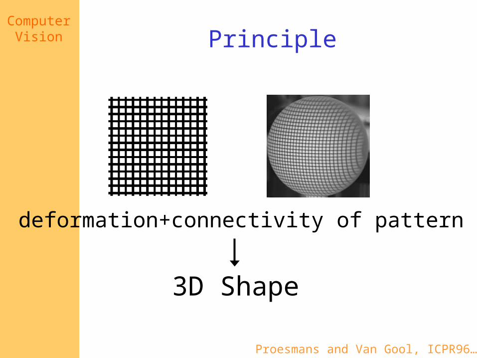
ComputerVision Principle
deformation+connectivity of pattern
3D Shape
Proesmans and Van Gool, ICPR96…

ComputerVision Acquisition setup
Proesmans and Van Gool, ICPR96…

ComputerVision Calibration
Proesmans and Van Gool, ICPR96…

ComputerVision Image with projected grid
Proesmans and Van Gool, ICPR96…

ComputerVision Line detectors
Proesmans and Van Gool, ICPR96…

ComputerVision Linking
Proesmans and Van Gool, ICPR96…

ComputerVision Initial grid
Proesmans and Van Gool, ICPR96…

ComputerVision Corrected grid
sub-pixel refinement of grid
Proesmans and Van Gool, ICPR96…

ComputerVision Depth computation
Proesmans and Van Gool, ICPR96…

ComputerVision Removing lines
Proesmans and Van Gool, ICPR96…

ComputerVision Texture estimation
Proesmans and Van Gool, ICPR96…

ComputerVision 3D Reconstruction
Proesmans and Van Gool, ICPR96…

ComputerVision Dionysos
Proesmans and Van Gool, ICPR96…
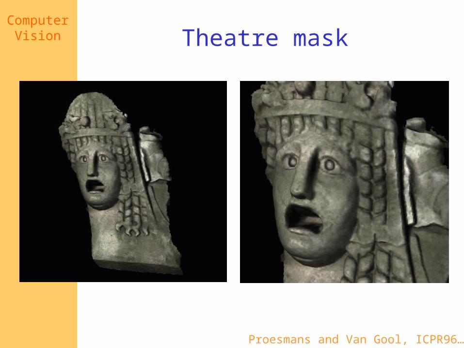
ComputerVision Theatre mask
Proesmans and Van Gool, ICPR96…

ComputerVision Capital
Proesmans and Van Gool, ICPR96…

ComputerVision Coded planes
• Structured light: – Use projector as a camera– Figure out correspondences by coding light pattern– Only need to code 1D
(but not parallel with epipolar lines!)
B. Curless

ComputerVision A desktop scanner

ComputerVision

ComputerVision
ComputerVision

ComputerVision

ComputerVision

ComputerVision

ComputerVision

ComputerVision

ComputerVision
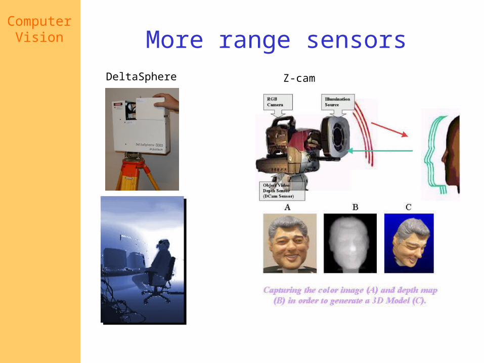
ComputerVision More range sensors
DeltaSphere Z-cam
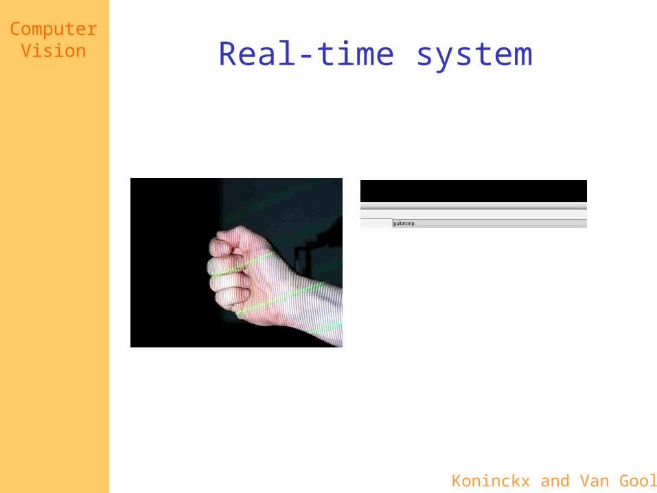
ComputerVision Real-time system
Koninckx and Van Gool

ComputerVision
Elements of Analytical Differential Geometry
• Parametric surface: x : U RR2 EE3
• Unit surface normal: N = (xu x xv) | xu x xv |
1
• First fundamental form:
I( t, t ) = Eu’2 + 2Fu’v’+Gv’2
E=xu . xu
F=xu . xv
G=xv . xv
{• Second fundamental form:
II( t, t ) = eu’2 + 2fu’v’+gv’2
e= – N . xuu
f = – N . xuv
g= – N . xvv
{• Normal and Gaussian curvatures:
t = I( t, t )
II( t, t )K =
eg – f 2
EG – F 2

ComputerVision
(1+hu2+hv
2)2
huuhvv–huv2
And the Gaussian curvature is: K = .
Example: Monge Patches
h
u
v
x ( u, v ) = (u, v, h( u, v ))
In this case
• N= ( –hu , –hv , 1)T
• E = 1+hu2; F = huhv,; G = 1+hv
2
• e = ; f = ; g =
(1+hu2+hv
2)1/2
1
(1+hu2+hv
2)1/2
–huu
(1+hu2+hv
2)1/2
–huv
(1+hu2+hv
2)1/2
–hvv
ComputerVision
uv
N
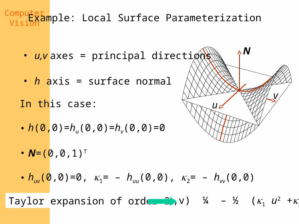
Example: Local Surface Parameterization
• u,v axes = principal directions
• h axis = surface normal
In this case:
• h(0,0)=hu(0,0)=hv(0,0)=0
• N=(0,0,1)T
• huv(0,0)=0, 1= – huu(0,0), 2= – hvv(0,0)
h(u,v) ¼ – ½ (1 u2 +2 v2)Taylor expansion of order 2

ComputerVision Finding Step and Roof Edges in Range Images
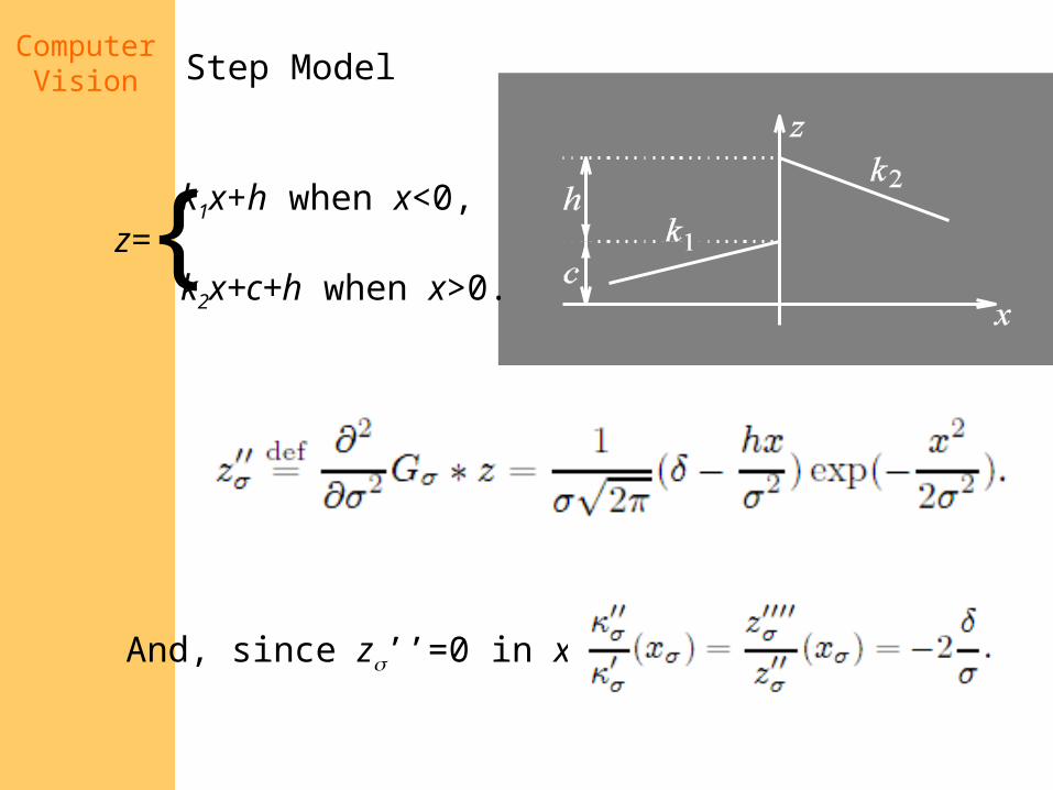
ComputerVision Step Model
k1x+h when x<0,
k2x+c+h when x>0.{z=
And, since z’’=0 in x :
ComputerVision
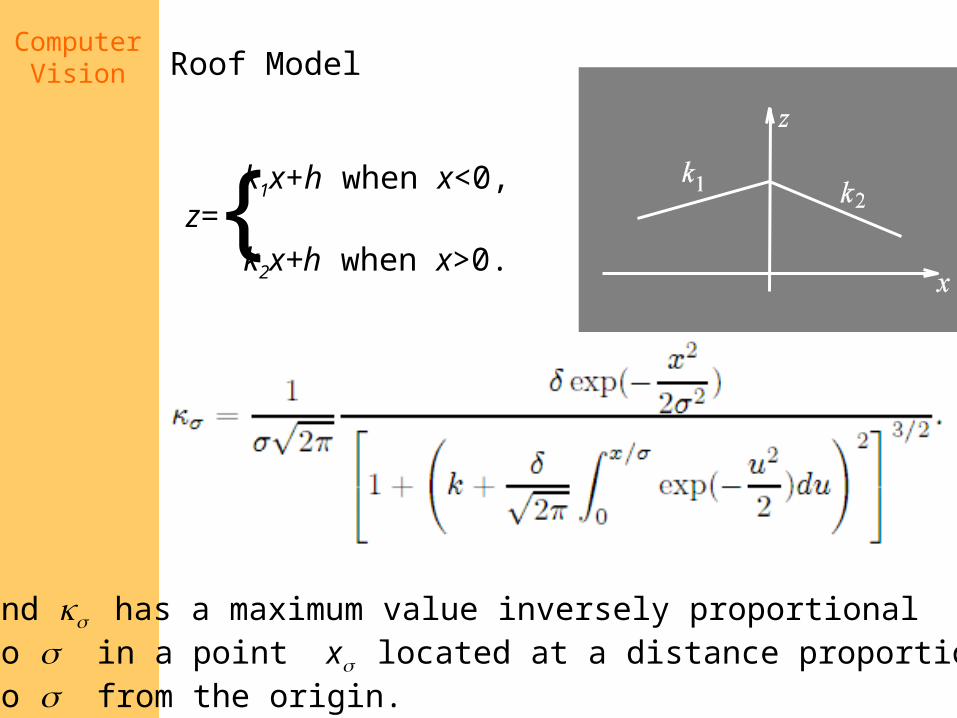
k1x+h when x<0,
k2x+h when x>0.{z=
Roof Model
And has a maximum value inversely proportionalto in a point x located at a distance proportionalto from the origin.
ComputerVision
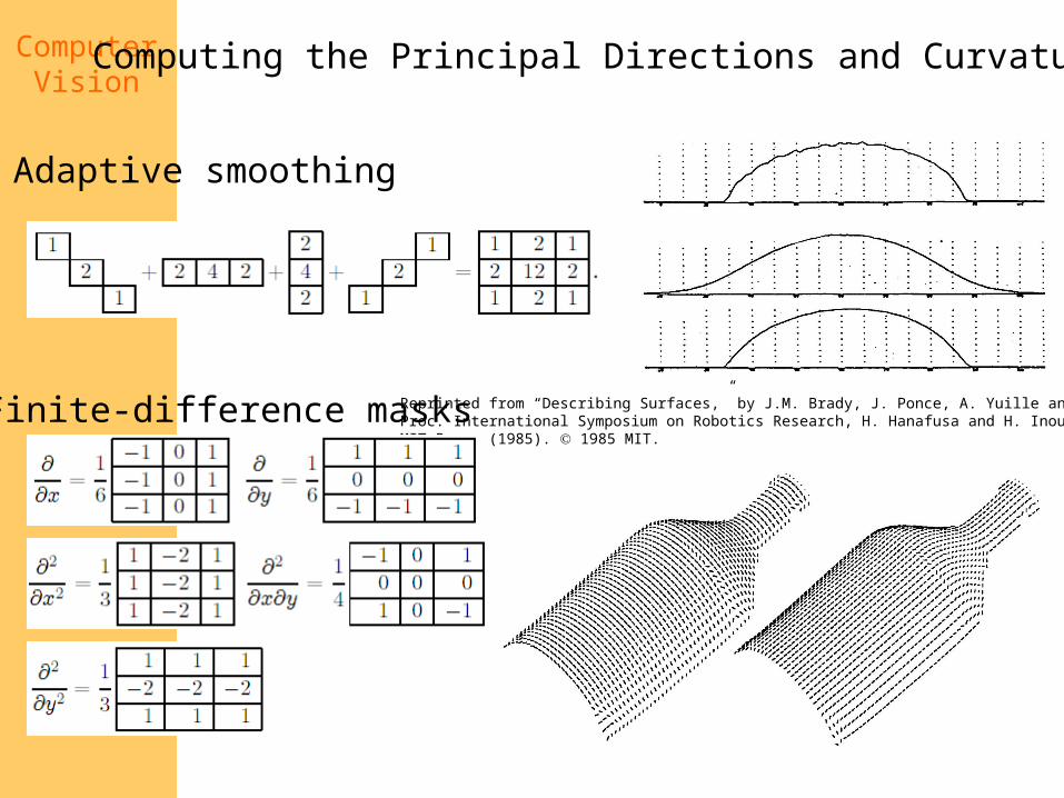
Computing the Principal Directions and Curvatures
• Adaptive smoothing
• Finite-difference masks Reprinted from “Describing Surfaces,” by J.M. Brady, J. Ponce, A. Yuille and H. Asada,Proc. International Symposium on Robotics Research, H. Hanafusa and H. Inoue (eds.),MIT Press (1985). 1985 MIT.

ComputerVision
Scale-SpaceMatching
Reprinted from “Toward a Surface Primal Sketch,”By J. Ponce and J.M. Brady, in Three-DimensionalMachine Vision, T. Kanade (ed.), Kluwer AcademicPublishers (1987). 1987 Kluwer Academic Publishers.

ComputerVision
Segmentation into Planes via Region Growing(Faugeras & Hebert, 1986)
Idea: Iteratively mergethe pair of planar regionsminimizing the averagedistance to the plane bestfitting them.
Reprinted from “The Representation, Recognition and Locating of 3D Objects,” by O.D. Faugeras and M. Hebert, the International Journal of Robotics Research, 5(3):27-52 (1986). 1986 Sage Publications. Reprinted by permission of Sage Publications.

ComputerVision
Quaternions
q = a + q is a quaternion,a 2 RR is its real part, and 2 RR3 is its imaginary part.
• Sum of quaternions: ( a+ ) + ( b+ ) ´ ( a+b ) + (+ )
• Multiplication by a scalar: ( a+ ) ´ ( a+ )
• Quaternion product:
( a+ ) ( b+ ) ´ ( a b – ¢ ) + ( a + b + £ )
• Conjugate: q = a + ) q ´ a –
Operations on quaternions:
• Norm: | q |2 ´ q q = q q = a2 + | |2
Note: | qq’|= |q| |q’|

ComputerVision Quaternions and Rotations
• Let R denote the rotation of angle about the unit vector u.
• Define q = cos /2 + sin /2 u.
• Then for any vector , R = q q.
Reciprocally, if q = a + ( b, c, d )T is a unit quaternion, the corresponding rotation matrix is:

ComputerVision The Iterative Closest Point Registration Algorithm
(Besl and McKay, 1992)
Key points:• finding the closest-point pairs (k-d trees, caching);• estimating the rigid transformation (quaternions).

ComputerVision
Using Quaternions to Estimate a Rigid Transformation
Problem: Find the rotation matrix R and the vector t that minimize
i=1E = | xi’ – R xi – t |2 .
n
At a minimum: 0 = E/ t = –2 ( xi’ – R xi – t ) .n
i=1
Or.. t = x’ – R x.
If yi = xi –x and yi’ = xi’ –x’, the error is (at a minimum):
i=1E = | yi’ – R yi |2
n
i=1= | yi’ q – q yi |2
n
i=1 = | yi’ – q yi q|2|q|2
n
Or.. E = AiT Ai with Ai =
0 yiT-yi’T
yi’-yi [yi+yi’]£
Linear least squares !!

ComputerVision ICP Registration Results
Reprinted from “A Method for Registrationof 3D Shapes,” by P.J. Besl and N.D. McKay,IEEE Trans. on Pattern Analysis and MachineIntelligence, 14(2):238-256 (1992). 1992 IEEE.
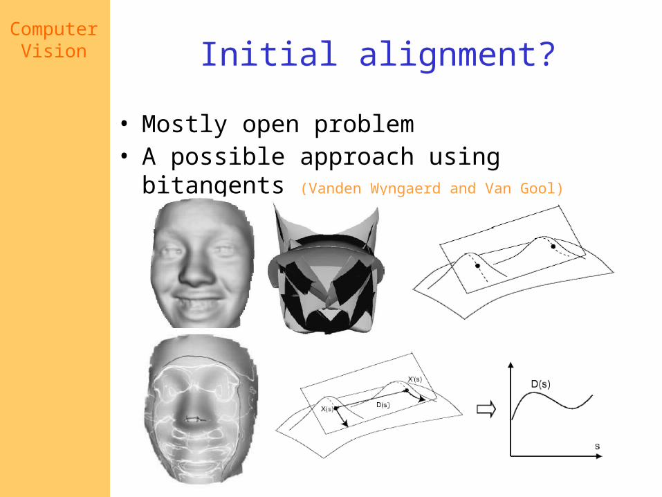
ComputerVision Initial alignment?
• Mostly open problem• A possible approach using bitangents
(Vanden Wyngaerd and Van Gool)

ComputerVision

ComputerVision

ComputerVision
ComputerVision
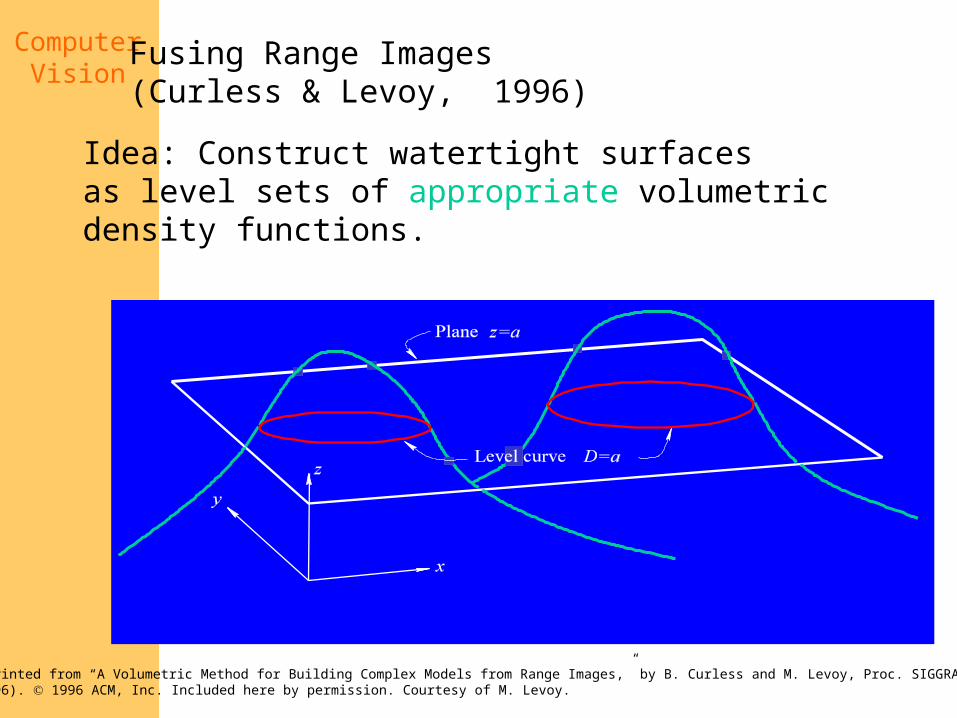
Fusing Range Images(Curless & Levoy, 1996)
Idea: Construct watertight surfacesas level sets of appropriate volumetricdensity functions.
Reprinted from “A Volumetric Method for Building Complex Models from Range Images,” by B. Curless and M. Levoy, Proc. SIGGRAPH (1996). 1996 ACM, Inc. Included here by permission. Courtesy of M. Levoy.
ComputerVision
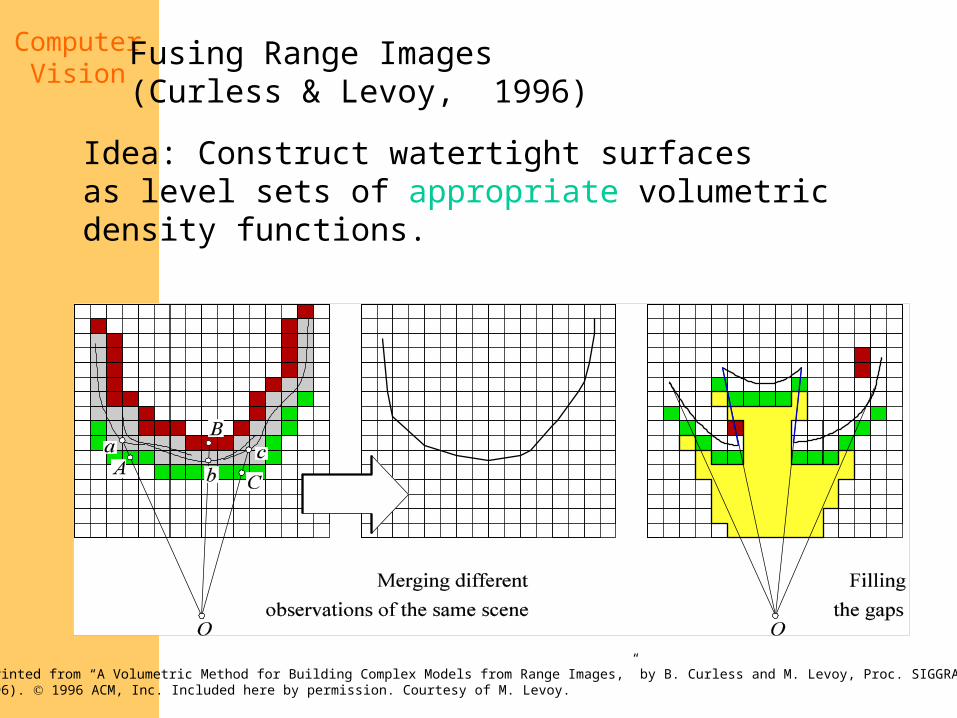
Fusing Range Images(Curless & Levoy, 1996)
Idea: Construct watertight surfacesas level sets of appropriate volumetricdensity functions.
Reprinted from “A Volumetric Method for Building Complex Models from Range Images,” by B. Curless and M. Levoy, Proc. SIGGRAPH (1996). 1996 ACM, Inc. Included here by permission. Courtesy of M. Levoy.

ComputerVision Volumetric integration
(Curless and Levoy, Siggraph´96)
sensor
range surfaces
volume
distance
depth
weight(~accuracy)
signed distanceto surface
surface1
surface2
combined estimate
• use voxel space• new surface as zero-crossing (find using marching cubes) • least-squares estimate (zero derivative=minimum)

ComputerVision
Fusing Range Images(Curless & Levoy, 1996)
Idea: Construct watertight surfacesas level sets of appropriate volumetricdensity functions.
Reprinted from “A Volumetric Method for Building Complex Models from Range Images,” by B. Curless and M. Levoy, Proc. SIGGRAPH (1996). 1996 ACM, Inc. Included here by permission. Courtesy of M. Levoy.

ComputerVision
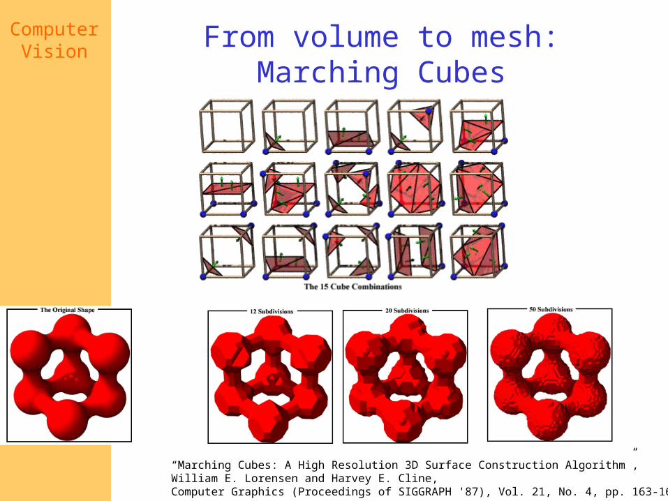
From volume to mesh:Marching Cubes
• First 2D, Marching Squares
“Marching Cubes: A High Resolution 3D Surface Construction Algorithm”,William E. Lorensen and Harvey E. Cline,Computer Graphics (Proceedings of SIGGRAPH '87), Vol. 21, No. 4, pp. 163-169.
ComputerVision
From volume to mesh:Marching Cubes
“Marching Cubes: A High Resolution 3D Surface Construction Algorithm”,William E. Lorensen and Harvey E. Cline,Computer Graphics (Proceedings of SIGGRAPH '87), Vol. 21, No. 4, pp. 163-169.

ComputerVision
From volume to mesh:Marching Cubes
• Improvement
“Marching Cubes: A High Resolution 3D Surface Construction Algorithm”,William E. Lorensen and Harvey E. Cline,Computer Graphics (Proceedings of SIGGRAPH '87), Vol. 21, No. 4, pp. 163-169.

ComputerVision The Faugeras-Hebert Plane Matching Algorithm (1986)
Key points:• finding initial matches (area comparisons, binning);• estimating the rigid transformation (quaternions).

ComputerVision Finding all the vectors v making an angle between -
And + with a vector u.

ComputerVision
Using Quaternions to Estimate a Rigid Transformation
Linear least squares !!
: n ¢ x – d = 0 ! ’: n’ ¢ x’ – d’ = 0
where n’ = R n and d’ = n’ ¢ t + d.
i=1
Problem: Find the rotation matrix R and the vector t that minimize
i=1Er = | ni’ – R ni |2
n
Et = | di’ – di – ni’¢ t |2. n
and

ComputerVision Recognition Results
(Faugeras & Hebert, 1986)
Reprinted from “The Representation, Recognition and Locating of 3D Objects,” by O.D. Faugeras and M. Hebert, the International Journal of Robotics Research, 5(3):27-52 (1986). 1986 Sage Publications. Reprinted by permission of Sage Publications.

ComputerVision
Spin Images (Johnson & Hebert, 1998)
SP(Q)=(|PQ£ n|, PQ¢ n)

ComputerVision
Reprinted from “Using Spin Images for Efficient Object Recognition from Cluttered 3D Scenes,” by A.E. Johnson and M. Hebert, IEEE Trans. on Pattern Analysis and Machine Intelligence, 21(5):433-449 (1999). 1999 IEEE.
Sample SpinImages
Matching Criterion:

ComputerVision
Recognition Results
Reprinted from “Using Spin Images for Efficient Object Recognition from Cluttered 3D Scenes,” by A.E. Johnson and M. Hebert,IEEE Trans. on Pattern Analysis and Machine Intelligence, 21(5):433-449 (1999). 1999 IEEE.
ComputerVision Computer Vision
• What next?
• Related courses:– Comp 254 Image Analysis (Spring)– Comp 255 Recent Advances in Image Analysis
(Odd Falls)
– Comp 290 3D photography?

ComputerVision The future is bright
• Computation is cheap• Lots of pix
– cameras are cheap, many pix are digital• Lots of demand for “slicing and dicing” pix
– generate models– new movies from old– search
• Lots of “hidden value”– can’t do data mining for collections with pix in
them• e.g. mortgage papers, cheques, etc.• e.g. filtering

ComputerVision There are lots of cameras!
surveillance cameras~1500/sq.mile in Manhattan
ComputerVision Recent flowering of vision
• can do (sort of!)– structure from
motion– segmentation– video representation– model building– tracking– face finding
• will be able to do (sort of!)– face recognition– inference about
people– character
recognition– perhaps more

ComputerVision Big open problems
• Next step in structure from motion
• Really good missing variable formalism
• Decent understanding of illumination, materials and shading
• Segmentation
• Representation for recognition
• Efficient management of relations
• Recognition processes for lots of objects
• A lot of this looks like applied statistics

ComputerVision Next week:
Final project presentations