contract no. w-7^05-eng-26

Contract No. W-7^05-eng-26

Neutron Physics Division

ELECTROMAGNETIC PRODUCTION OF PION PAIRS

CD. Zerby

Date Issued

OAK RIDGE NATIONAL LABORATORY

Oak Ridge, Tennesseeoperated by

UNION CARBIDE CORPORATION

for the

U.S. ATOMIC ENERGY COMMISSION

ORNL-3033

Si)iliiJii,iiNiEfSS!j?-=«TOs

3 445b 03t4eiS

ii

ABSTRACT

The suggestion that the electromagnetic production of pion pairs

may be a possible way of investigating the it-n interaction has stimulated

this study of the Pauli-Weisskopf theory of pair production in the experi

mentally attainable region just above threshold. The Pauli-Weisskopf

theory was investigated with the objective of including the strong pion-

nucleus interaction in the form of a complex optical potential as a means

of determining the increase in the cross section resulting from this

interaction. It was found that the potentials could be included in the

field equations in a consistent manner that would lead to the absorption

and scattering of the pions after production if the real part of the

potential were a world scalar and the imaginary part the time component

of a four-vector. The matrix element for pair production was obtained

by using exact waves which were expanded into angular momentum states,

and numerical calculations were performed to examine the effect of a

nuclear charge distribution and nuclear potential on the cross section.

In the region just above threshold it was found that the cross section

for lead with a charge distribution of the form obtained from electron

-1+scattering experiments was approximately a factor 10 smaller than that

obtained with a point charge nucleus and that this reduction in the cross

section was regained when a nuclear optical potential was included that

has a depth consistent with pion scattering experiments. The calculations

show that the cross section for lead with a charge distribution and nuclear

optical potential increases slowly just above threshold until approximately

295 Mev, where it starts to increase almost linearly, attaining a value

of 1.07 x 10"52 cm2 at 310 Mev.

iii

ACKNOWLEDGMENTS

The author is deeply indebted to Dr. T. A. Welton, who suggested

this problem and under whose guidance it was carried out. The many

stimulating discussions with him which were possible only by a generous

allocation of his time contributed markedly to every phase of this work.

The author is also grateful to the administration of the Oak Ridge

National Laboratory, who made their facilities available in the comple

tion of the work, and is particularly appreciative of the consideration

of the Director of the Neutron Physics Division, Mr. E. P. Blizard, for

arranging the work schedule so that this problem could be considered and

carried to completion.

TABLE OF CONTENTS

CHAPTER PAGE

I. INTRODUCTION ...................... 1

History of Problem ....... . 2

Objectives of the Study . 5

Organization of the Report .............. 6

Notations and Units . ........ 7

II. GENERAL CONSIDERATIONS ............ 8

The Charge Distribution ................. 8

The Heavy-Nucleus Approximation ............ 12

III. THE OPTICAL POTENTIAL AND ITS INTRODUCTION

INTO THE FIELD EQUATIONS lfc

Justification of the Optical Model .......... Ik

Introduction of the Complex Optical Potential

into the Field Equations ........ 17

IV. FORM OF THE FINAL-STATE FUNCTIONS 27

V. DEVELOPMENT OF THE PAIR PRODUCTION CROSS SECTION

IN ANGULAR MOMENTUM STATES .............. 3^

VI. METHODS OF SOLUTION h8

General Description of Contents ............ kQ

Racah and Clebsch-Gordon Coefficients . . U9

Methods for Obtaining the Function F(£.£n£JL,) ..... 5112 3

Spherical Bessel functions ............. 51

The Coulomb potential ................ 52

VI

CHAPTER PAGE

Removing the singularity in the radial differential

equation 5^

Solution of the radial differential equation .... 56

Determination of the normalizing constant and complex

phase shift 58

Performing the integration in F^i^L) 62

The General Plan of the Calculation 6h

VII. RESULTS 67

Calculations with the Coulomb Potential 67

The Born approximation ..... 67

Comparison of Born approximation and calculations

with exact waves 71

Calculations with a Modified Coulomb and Nuclear

Potential 76

VIII. SUMMARY 83

BIBLIOGRAPHY 88

APPENDIX A 93

APPENDIX B 98

APPENDIX C 100

vii

LIST OF TABLES

TABLE PAGE

I. The Pion Pair Production Cross Section in Units

of OR2 = 7.762 x 10~55 cm for Lead, Including

the Coulomb and Optical Potential 80

IX

LIST OF FIGURES

FIGURE PAGE

1. Values of the Real Part of a Square-Well Optical Potential

as Determined from Pion-Nucleus Scattering Data 18

2. Values of the Imaginary Part of a Square-Well Optical Potential

as Determined from Pion-Nucleus Scattering Data 19

3. Comparison of the Born Approximation Pion Pair Production Cross

Section at a Photon Energy of 310 Mev for a Point-Charge

and Distributed-Charge Lead Nucleus 70

h. Comparison of the Born Approximation and Exact Wave Pion Pair

Production Cross Section for Lead at a Photon Energy of

290 Mev. The Nuclear Potential Was Neglected 72

5. Comparison of the Born Approximation and Exact Wave Pion Pair


300 Mev. The Nuclear Potential Was Neglected 73

6. Comparison of the Born Approximation and Exact Wave Pion Pair


310 Mev. The Nuclear Potential Was Neglected Jk

7- Ratio of Exact Wave to Born Approximation Differential Cross

Section as a Function of Z for Photon Energy of 290 Mev . . 75

8. Ratio of Exact Wave to Born Approximation Pion Pair Production

Cross Section for Lead as a Function of Energy. The Nuclear

Potential Was Neglected 77

9. The Differential Pion Pair Production Cross Section for Lead

Including the Coulomb and Nuclear Optical Potential

(P = -16 Mev, V = -5 Mev) 79

FIGURE PAGE

10. The Pion Pair Production Cross Section for Lead Including

the Coulomb and Nuclear Optical Potential (P = -16 Mev,

V = -5 Mev) as a Function of Photon Energy 82

CHAPTER I

INTRODUCTION

The Pauli-Weisskopf theory of the electromagnetic production of

pion pairs has been a subject of interest in various connections for many

years. Recently new interest has been stimulated in the theory because

pion pair production is a possible means of investigating the it-it inter-

2action. This approach, which was originally suggested by Pomeranchuk,

is particularly valid in view of the increase in the cross section, when

the strong pion-nucleus interaction is included, over that obtained by

the original theory. The purpose of this work was to study the Pauli-

Weisskopf theory with the objective of including the strong pion-nucleus

interaction and developing an accurate method of obtaining the cross

section for pair production in the experimentally attainable energy

region. The it-it interaction was neglected in this work since there is

insufficient information available at the present time to adequately

treat this interaction.

"Sf. Pauli and V. Weisskopf, Helv. Phys. Acta 7, 709 (193*0.

Iu. la. Pomeranchuk, Doklady Acad. Nauk S. S. S. R. 96, 265 andl+8l (I95I+); English translation: Proceedings of the Cern SymposiumI956 (Service d'Information, Cern, 1956), vol. II, p. 167.

I. HISTORY OF PROBLEM

3Shortly after Bethe and Heitler derived the cross-section formula

for the electromagnetic production of electron pairs in 193^, Pauli and

Weisskopf evolved a similar expression, starting with a complex scalar

field and using the methods of second quantization, for the production

of charged pairs of Bose particles.

The Pauli-Weisskopf theory is particularly interesting since it

was the first method of treating a problem where the equations of motion

are given by the Klein-Gordon equation. This equation had been a subject

of much dispute and little use before the Pauli-Weisskopf theory appeared,

because the probability density obtained in the same manner as in non-

relativistic quantum mechanics led to a quantity which was not positive-

definite .

As in the Bethe-Heitler derivation, Pauli and Weisskopf had

assumed that the pair production took place in the presence of an

infinitely heavy charged nucleus and had considered the Coulomb inter

action as part of the perturbation. This meant that the Fourier

coefficients of the field satisfied the Klein-Gordon equation without

the Coulomb potential and therefore could be expanded in a series of

plane waves. This method of quantization was not a necessary condition,

kas was demonstrated by Snyder and Weinberg, who showed that the

Hamiltonian could be brought to diagonal form by a unitary transformation

when an electrostatic field is present. From this it can be shown that

_

H. Bethe and W. Heitler, Proc. Roy. Soc. (London) AlU6, 83 (193*0-

H. Snyder and J. Weinberg, Phys. Rev. 57, 307 (19^0).

the second-order perturbation theory used by Pauli and Weisskopf could

be relaxed to a first-order process where the perturbation was the

interaction between the complex scalar field and the electromagnetic

field. In this case the Fourier coefficients could be expanded in a

series of exact waves.

Although the interest in the Pauli-Weisskopf theory as a tool to

help investigate nuclear forces had been extensive, it was not until the

5discovery of the « mesons in 19^+7 by Lattes, Occhialini, and Powell

6and the subsequent determination of their properties that the theory

was known to apply to physical particles. The spin zero of the it mesons

and their appearance in positive- and negative-charged states with

approximately the same rest mass clearly indicated that the theory was

directly applicable and appropriate to use for the determination of the

cross section for the electromagnetic production of charged pion pairs.

An essential element of the Pauli-Weisskopf theory of pair pro

duction was the presence of the Coulomb field, which provided a means of

interaction between the meson field and the nucleus to transmit linear

momentum to the nucleus, thereby enabling energy and momentum in the

pair production process to be conserved. However, the Coulomb field

is not the only method of interaction since there exists a strong,

nonelectromagnetic interaction between the meson field and the nucleon

5Lattes, Occhialini, and Powell, Nature 160, U53, kQ6 (19^7).

H. A. Bethe and F. de Hoffmann, Mesons and Fields (Row, Petersonand Company, Evanston, 1955), vol. II, sec. 27 and 20.

'It is assumed that the nucleus is infinitely heavy, so that noenergy is transmitted to the nucleus.

Q

field. Landau and Pomeranchuk were the first to introduce the strong

interaction into the theory of meson bremsstrahlung in a semiphenomeno-

logical way by means of an optical model for the nucleus. Using the

2same approach, Pomeranchuk later introduced the optical model into the

theory for meson pair production. In both cases the nucleus was assumed

to be "black" to mesons with a cross-sectional area equal to the total

inelastic cross section for incident mesons. In this manner Pomeranchuk

arrived at the pair production cross section which would leave the

nucleus in an unexcited state.

9 10Vdovin/ using the optical model of Fernbach, Serber, and Taylor,

extended Pomeranchuk's work to include the strong pion-nucleon inter

action in the form of a gray nucleus. Both Pomeranchuk and Vdovin

neglected the Coulomb field in their derivations and used a high-

energy approximation.

The inclusion of the strong interaction in the theory is an

important feature since the cross section for pair production is very

small, considering only the modified Coulomb potential from a finite

nucleus which is necessary in this theory; the strong interaction makes

the pair production much larger and therefore is of considerable interest

since pair production is a possible means of investigating the jt-it

interaction.

8L. D. Landau and Iu. la. Pomeranchuk, Zhur. Eksptl. i Teort. Fiz.

2k, 505 (1953); English translation: Proceedings of the Cern Symposium1956 (Service d'Information, Cern, 1956), vol. II, p. 159.

o

^Yu. A. Vdovin, Doklady Akad. Nauk S. S. S. R. 105, 9^7 (1955).

Fernbach, Serber, and Taylor, Phys. Rev. 75, 1352 (19^9).

II. OBJECTIVES OF THE STUDY

The optical model of Fernbach, Serber, and Taylor used by Vdovin

is based on the hypothesis that a complex optical potential can be

introduced into the equations of motion for the pions. The potential

was not explicitly introduced by Vdovin and this is a necessary step

for further, more exact, calculations of the cross section. Since it

is desirable ultimately to calculate the cross section as accurately as

possible, one objective of this work was to investigate the introduction

of such a potential into the field theoretical equations and to show

that it leads, in a consistent manner, to the absorption and scattering

of the pions after they are produced. The absorptive part of the

potential is intended to include, in a phenomenological way, all

inelastic events that leave the nucleus in an excited state. It acts

to remove the pions that have been produced within the nucleus which,

in effect, reduces the cross section, in addition to facilitating the

momentum transfer to the nucleus.

A second objective was to find a practical method of calculating

the matrix elements that arise in the formulation of the pair production

cross section. Matrix elements of this type, which involve integrals

where the integrand is a product of only continuum wave functions or

their derivatives, arise in many cases and are particularly difficult

to calculate. An accurate method of treating this problem with a

minimum amount of work would find many applications not only for

calculating matrix elements but also in other fields--for example, to

obtain the Fourier transforms of slowly converging oscillating functions.

2 9Since Pomeranchuk and Vdovin neglected the Coulomb interaction

in their work and used a high-energy approximation which effectively

placed their results in an energy range above that now attainable, an

additional objective of this study was to investigate the effects of

the distributed nuclear charge and the complex optical potential on the

total and differential cross section in the experimentally attainable

energy region just above threshold.

III. ORGANIZATION OF THE REPORT

Some of the general features of pion pair production, such as

consideration of a nucleus with a charge distribution and justification

of the heavy-nucleus approximation, are discussed in Chapter II.

Chapter III presents the justification of the use of the optical model

in the pair production and shows that the complex optical potential can

indeed be introduced into the field equations in a consistent manner.

In Chapter IV it is shown that the use of the complex optical potential

leads to an ambiguity of the form of the final-state wave functions in

the matrix elements and that this ambiguity can be resolved. The final

set of equations for the wave functions is then expanded into angular

momentum states in Chapter V, and the matrix element is shown to be

reducible in a convenient manner for final numerical calculations. The

methods devised for evaluating the various factors appearing in the

matrix element are given in Chapter VI; the results of some calculations

for lead showing the effects of the modified Coulomb potential and

nuclear optical potential on the cross section are presented in

Chapter VII.

IV. NOTATIONS AND UNITS

In most of this work the "natural units" n = c = 1 are used, and

when the ordinary units are used, they are so specified. In most cases

the notation is in a familiar form and needs no further clarification.

An exception to this perhaps is the notation used in Chapter III, where

the notation and conventions used by Schweber et al. in their book have

been carefully adhered to. The arguments of functions are omitted alto

gether when there is little likelihood of misunderstanding; in some cases

the arguments are included in the first step of a derivation and omitted

subsequently in order to simplify the notation. The major problem of

duplication of symbols could not be avoided. Where duplications appear,

the symbols are redefined.

In general, m without a subscript represents the pion mass, *. = —

2 2e e ^

the Compton wave length, a = t— the fine structure constant, R = —- = Q0C<nc mc^

the classical pion radius, and the electronic charge e was taken as a

positive quantity. In those sections where •& = c = 1, u is the mass of

the pion, <0) is an energy, and k and q are momenta.

Schweber, Bethe, and de Hoffmann, Mesons and Fields (Row,Peterson and Company, Evanston, 1955), vol.-T.

8

CHAPTER II

GENERAL CONSIDERATIONS

Before gDing on to a systematic development of the cross section

for the electromagnetic production of pion pairs which includes the

strong interaction in the form of an optical potential, it is necessary

to review some of the assumptions and general features of the theory.

It is particularly important to discuss the necessity of including a

nucleus with a charge distribution and also to review the heavy-nucleus

assumption.

I. THE CHARGE DISTRIBUTION

The electromagnetic production of pion pairs differs from the

production of electron pairs in one important way not previously

indicated: Because the mass of the pion is so much greater than that

of the electrons (approximately 273 electron rest mass units), the

production of the mesons takes place predominantly inside the nucleus.

This can be demonstrated by investigating the second-order perturbation

theory of Pauli and Weisskopf and assuming for the moment that the

2nucleus is a point charge. In the matrix element for the Coulomb

potential in the second-order perturbation theory an integral of the form

"Hf. Pauli and V. Weisskopf, Helv. Phys. Acta 7, 709 (193*0.o

The following analysis parallels the methods presented in thebook by W. Heitler, Quantum Theory of Radiation (Oxford University Press,London, 195*0, 3rd ed., p. 2kQ. ~

ik tn ^

: d^r (2.1)

occurs, where k is the momentum transferred to the nucleus. The mainn

contribution to this integral comes from a radius

1

ro~F(2.2)

n

since for distances greater than r the exponential function oscillatesu

rapidly for small changes in r" , and for distances less than r the

volume element d r is small. The radius r can therefore be interpreted

as the mean radius at which production takes place. The maximum value

of r^ is obtained when k has its minimum value which can easily be0 n

determined from the requirements of conservation of energy and linear

momentum consistent with the heavy-nucleus approximation. For fixed

magnitudes of q, the momentum of the incident photon, and 5+ and k_ ,

the momentum of the it and n~ mesons, respectively, we must have

t =-q- -£ . -£_ , (2.3)n y +

where the minimum magnitude of k from this expression occurs when

k = q - k - k_ . (2.10n y +

Allowing k and k to be variable but consistent with the conservation of

r^—2energy to = Co + o) > where k+ = .6d - u , we obtain the minimum value

of Eq. (2.10 when &)+ = a) = 1/2 &> = to and k+ =k_ = k, which gives

2

kQ(min) =q.y -2k =2{to - k) =2̂ L • (2.5)

10

Using k (min) for k in Eq. (2.2) we find that

r0(max) =<̂ , (2.6)-13

where JL is the meson Compton wavelength (l.k x 10 cm). For photon

energies just above threshold, U> ^ u and k = 0; therefore the main

contribution to pair production takes place less than 1 pion Compton

wavelength from the center of the nucleus, which is well within the

bounds of the nucleus.

Because the pair production may take place primarily inside the

nucleus, it is necessary to consider the finite extent of the nuclear

charge distribution. The results of the analysis of electron scattering

experiments from nuclei provide a convenient function to use in the form

of the distribution function

1+exp (-5-E;

which is reasonably close to the actual charge distribution for medium-

3heavy and heavy nuclei. The constant o is for normalization, and the

-13constants for the best fit to the experimental data are a = 0.5*<-6 x 10

cm and p=1.07 A1/5 x 10"15 cm.

Although the use of the charge distribution will lead to some

complications from a numerical standpoint, several advantages are

realized which outweigh the disadvantage. It was first pointed out by

Schiff et al. that when a modified Coulomb potential is sufficiently

\. Hofstadter, Revs. Mod. Fhys. 28, 2lU (1956).

Schiff, Snyder, and Weinberg, Phys. Rev. 5J_, 315 (19*^0:

11

broad in a region where its magnitude is greater than the rest mass

energy of the pion, the wave equation leads to complex eigenvalues for

certain states; in fact, the Hamiltonian with the modified Coulomb

potential present could not be brought to diagonal form. For the dis

tributed charge nucleus this problem is avoided, as can be seen if a

uniform charge distribution which approximates the distribution given

in Eq. (2.7) is examined. In this case the maximum value of the

potential well occurs at r = 0 and has the value

2

V(0)=^|- , (2.8)

where R is the nuclear radius and will be taken as approximately

^CA ' , with X the pion Compton wavelength. Then

o

y(0) V^216 /V _3ZoX ^3 ja , j

where a is the fine structure constant and we see that too deep a

Coulomb potential is never realized.

Another problem avoided by the charge distribution is the one

that occurs in the Klein-Gordon radial equations. The radial differ

ential equations with a point charge are of the form

x2

dr

P(r) +M -*(/+!> = 0 , (2.10)

where P(r) goes to infinity as l/r as r approaches zero; therefore, for

small r, we keep only the second term in the square brackets of Eq. (2.10)s+1

and seek solutions of the form Ar , which leads to

s=-I±i ,[(2l +if -k(Zaf . (2.11)

12

The choice of solutions from Eq. (2.11) is based on the boundary con

dition that 0(0) = 0 which is obtained for i > 0 by taking the upper

sign. However, for / = 0 and Za > 1/2, s is complex and the choice of5

solutions has to be made on other grounds. In any event the complex

power of r leads to complications when solving the radial equation, a

problem that can be avoided with the use of the distributed charge and

noting that the modified Coulomb potential from a charge distribution

is finite at the origin so that at small r the v term corresponding to2

(Za/r) in the differential equation can be dropped. The result s = £

is the desired solution.

II. THE HEAVY-NUCLEUS APPROXIMATION

In the Pauli-Weisskopf theory the assumption that the nucleus

is infinitely heavy means among other things that the cross section is

calculated in the center-of-mass frame of reference. In a physical

situation there is some interest concerning what corrections should be

made, if any, to transform from the laboratory to the center-of-mass

frame. Letting &) be the energy of the incident photon in the labora-

Q

tory frame, td the energy of the photon in the center-of-mass frame,

and M the rest mass of the nucleus, the transformation from 6J to 66

is given by

*o-M1 +-irJ • (2a2>

L. I. Schiff, Quantum Mechanics (McGraw-Hill Book Company, Inc.New York, 1955), 2nd ed., p. 322.

13

Therefore, for moderately heavy to very heavy nuclei there is little

cdifference between 4) and 6d until very high photon energies are

reached. In the region near threshold for lead the correction is

approximately 0.2$ and can be neglected. This means that the threshold

energy can be taken as twice the rest mass energy of the pions. Since

the pions have a rest mass equal to 273»27 electron rest mass units,

the threshold is at 279*17 Mev.

The assumption that the nucleus takes up no energy also warrants

a brief review here especially since the momentum transferred to the

nucleus is greater in the case of pion pair production than in electron

pair production. In a manner similar to that shown in Section I of this

chapter the maximum linear momentum transferred to the nucleus consistent

with negligible energy transfer is found to be

kn(max) -rf>0 +2^)2 -u2 , (2.13)

where u is the mass of the pion and 6) is the energy of the photon.

ergy transfer to the r

UL+ 2 Jk^2 -u2)*)(max)=^-2 * °—-i- , (2.H0

2M

where M is the mass of the nucleus. For lead and a photon energy of

290 Mev a maximum kinetic energy of 0.35 Mev is transferred to the

nucleus, which is a small percentage of the total energy available,

being only 3-2$ of the kinetic energy transmitted to the pions. At

higher photon energies these percentages decrease and the heavy nucleus

approximation seems to hold very well.

The maximum kinetic energy transfer to the nucleus is then approximately2

Ik

CHAPTER III

THE OPTICAL POTENTIAL AND ITS INTRODUCTION

INTO THE FIELD EQUATIONS

In the latter part of this chapter it is shown that an optical

potential can be introduced into the field equations in a consistent

manner; however, before entering into that discussion, it is appropriate

to review the optical model to establish its acceptability as a phenom-

enological means of introducing the scattering and absorption of pions

by a complex nucleus.

I. JUSTIFICATION OF THE OPTICAL MODEL

The "optical" model of the nucleus seems to have gained its name

from the model of Fernbach, Serber, and Taylor, in which they treated

the nucleus as a continuous medium with a complex index of refraction.

The model was so designated because of the similarity of the treatment

to the familiar methods in optics where an incident wave can be coherently

scattered and attenuated by a medium with a complex index of refraction.

Actually, the model of Fernbach, Serber, and Taylor is based on the

hypothesis that a complex interaction potential can be introduced into

the wave equation which depends only on the coordinates of the incident

particle relative to the nucleus as a whole. Only by means of a

potential of this type is one led to the concept that a complex index of

refraction will apply to the nucleus. For this reason it is customary

T'ernbach, Serber, and Taylor, Phys. Rev. 75, 1352 (19*4-9).

15

to refer to the complex potential for the nucleus as an optical

potential and to refer to the inclusion of the potential in the wave

equation as using an optical model.

2Bethe was the first to show the significance of a complex optical

potential some years before the model of Fernbach, Serber, and Taylor

appeared. He showed that the complex potential would introduce the

coherent scattering of an incident particle and that the imaginary part

of the potential was responsible for its absorption. 'The function of

the imaginary part of the potential as a means of introducing absorption

is very effectively demonstrated when the continuity equation is

derived from the Schrb'dinger wave equation as was done by Mott and

5Massey.

The optical model is not without some justification from a

1+microscopic point of view. In one series of papers treating the

multiple scattering of particles by complex nuclei, the multiple-

scattering formalism which leaves the nucleus in an unexcited state

was shown to ultimately lead to an optical potential. Although the

optical potential as derived by this method is not necessarily propor-

5tional to the density of nucleons, Frank, Gammel, and Watson showed

2.•H. A. Bethe, Phys. Rev. 57, 1125 (l9*+0).

5N. F. Mott and H. S. W. Massey, The Theory of Atomic Collisions(Oxford University Press, London, 19*^0), 2nd ed., p. 12.

Sc. M. Watson, Phys. Rev, 89, 575 (1953); N. C. Francis andK. M. Watson, Phys. Rev. 92, 291 "(1953); G. Takeda and K. M. Watson,Phys. Rev. 97, 1336 (19557T K. M. Watson, Phys. Rev. 105, 1388 (1957).

Frank, Gammel, and Watson, Phys. Rev. 101, 891 (1956).

16

explicitly that in the limit of large nuclei the proportionality is

obtained.

The optical potential and the optical model of Fernbach, Serber,

and Taylor have been useful tools for analyzing scattering data. Many

workers have presented their analysis of meson-nucleus scattering in

terms of these models and obtained reasonably good fits to the experi

mental data. In most cases the potential was assumed to be proportional

6to the nucleon density; however, in one case analyses were made with

7the more complicated Kisslinger potential based on Watson's multiple-

o

scattering theory.

One of the most significant results of the analysis of pion-

nucleus scattering relating to this work is that the real part of the

optical potential is attractive and of the same magnitude for both jt~

and it mesons. Also, inclusion of a complicated well shape and the

more complicated Kisslinger potential to obtain the correct back

scattering from light nuclei is not necessary for heavy nuclei such as

lead, which was used in this work. The assumption that the potential

is proportional to the nucleon density is very good for lead; in fact,

only a square-well potential need be used since the nucleon density is

almost uniform over much of the nuclear volume. An additional

g

References to the original papers on the scattering of mesonsfrom nuclei containing analyses in terms of a nuclear optical potentialproportional to the nucleon density are included in a paper by G. Saphir,Phys. Rev. 10*i_, 535 (1956).

7L. S. Kisslinger, Phys. Rev. o£, 761 (1955).

Baker, Rainwater, and Williams, Phys. Rev. 112, 1763 (1958).

17

justification for use of the square-well approximation for the nuclear

optical potential in this work is that the experimental data have an

uncertainty which does not warrant the use of a more detailed potential.

Values for the real and imaginary part of a square-well optical

potential which leads to a best fit of the low-energy experimental pion-

nucleus scattering data are given in Figures 1 and 2. The dashed curve

9reflects the analysis of Stork, who compared the low-energy data and the

high-energy data to determine which points were the most reliable. Al

though there are no data below an incident energy of 33 Mev to include in

Figures 1 and 2, it is reasonable to assume that the curves are flat in

this region. This assumption is based on the calculations of Frank,

5Gammel, and Watson, who obtained the potentials from the formulas

relating the optical potential to the multiple-scattering theory and

included the effects of the nucleon motion in the nucleus.

II. INTRODUCTION OF THE COMPLEX OPTICAL POTENTIAL

INTO THE FIELD EQUATIONS

Once the use of an optical potential was justified as a tool for

describing the coherent scattering and absorption of the pion pairs after

production occurs, the problem remaining was how to introduce dissipation

into the Pauli-Weisskopf theory which is normally nondissipative. Dissi

pation as used here is meant to refer to the absorption of particles by a

means such as the complex potential. In the analysis of pion-nucleus

scattering this problem did not arise because of the nature of the

process and because most of the analyses were done with a quasi-Schrodinger

9D. H. Stork, Phys. Rev. 93, 868 (195*0°

18

>0)

_l

<

LUh-O0_

<O

I-0_O

U_

O

I-rr

2

<UJrr

Figure 1

as

0

UNCLASSIFIED

0RNL-LR-DWG 52730

-10

-20

-30

< '

41

o

X\

v

I \l

O ST0RKa

-40• SAPIR0bA PEVSNER etal.c

e;r\

A BYFIELD eiaLd

I I

0 20 40 60

PION ENERGY (Mev)

80 100

. Values of the Real Part of a Square-Well Optical Potential

Determined from Pion-Nucleus Scattering Data.

aD. H. Stork, Phys. Rev. 93, 868 (1954).

bA. M. Sapiro, Phys. Rev. 84, 1063 (1951) and H. A. Bethe andR. R. Wilson, Phys. Rev._83, 690(1951).

cPevsner et al., Phys. Rev. 100, 1419 (1955).

dByfield, Kessler, and Lederman, Phys. Rev. 86, 17(1952).

-5 0

£ -10UJi-o

<O

h-0_O

U_o

-20

-30

UNCLASSIFIED

ORNL-LR-DWG 52731

or

<

S-. 0

"KviX

\\

T V0

o

O ST0RKa• SAPIR0bA PEVSNER et al°

A BYFIELD et al_d• SAPHIRe

I

-40 —

<

- -50

0 20 40 60

PION ENERGY (Mev)

80 100

19

Figure 2. Values of the Imaginary Part of a Square-Well OpticalPotential as Determined from Pion-Nucleus Scattering Data.

aD. H. Stork, Phys. Rev. 93, 868 (1954).

bA. M. Sapiro, Phys. Rev._84, 1063(1951) and H. A. Bethe andR. R. Wilson, Phys. Rev. 83, 690 (1951).

cPevsner etaL, Phys. Rev. 100, 1419(1955).

dByfield, Kessler, and Lederman, Phys. Rev. 86, 17 (1952).

eG. Saphir, Phys. Rev. 104, 535 (1956).

20

wave equation for it or it" mesons, where the potential was nominally the

time component of a four-vector. In pair production, however, great care

must be taken to assure that the optical potentials enter the field

equations in the proper way to obtain dissipation (absorption) of both

it and it~ mesons since they enter the theory in a symmetric way. In

addition, scattering experiments are essentially nonrelativistic,

whereas pair production is a relativistic phenomenon; therefore it is

essential that the relativistic aspects of the problem be maintained

throughout this study.

For purposes of discussing the proper form of the complex optical

potential in the field equations, it is necessary to introduce two real

world scalar potentials, P and P,, and a complex time component of a

four-vector V0» At first, to display the co-variance of the equations,

the potential V will be represented as a four-vector, and the space com

ponents will be set to zero at the end. With the potentials present in

the equations, the variation of the action for the complex scalar field

and electromagnetic field can be written as

&I =6 /i£dkx +/(QS0 +Q*hf) &kx =0 , (3.1)

where the Lagrangian density o£ must be a real function and is given

along with the field components Q and 0* by

(3.2)

V ox"

Q = 'JL-ieA^ Y* +VJ (£- -ieA^j-vV? +2i(u +P) ?± f >

(3-3)

Q* = ^-L. +leA \v? +y (£-+ieA^ -VV^ -2i(]i +P) Px

21

0 .

(3.M

This form of the variation of the action is patterned after the equation

that appears in classical mechanics when nonconservative forces are

present and will lead to a nonconservation of particles and charge.

Certain terms in Eq. (3«3) and (3A) can logically be included in the

Lagrangian density and will lead to the same results given below.

However, for purposes of simplicity, because of the convenient notation,

these terms are retained in the expressions for Q and Q*.

Performing the variation indicated in Eq. (3*1) leads to the

following equations of motion:

W ' ^W + Q = 0 , (3.5)

-£5-Dv-S • (">V

It should be noted that Eq. (3*7) gives the correct definition

for the current four-vector as

-3-v • (5-8)H. Goldstein, Classical Mechanics (Addison-Wesley Publishing

Company, Inc., Cambridge, 1953), p. 33.

22

which, in the present case, is

j = -ie (5-~/)'-'ft--v)! (3.9)

This expression will be useful later.

Equation (3.5) should be examined at this point to determine the

way that the potentials appear in the equations of motion. To this end,

Eqs. (3.2), (3.3), and (j.k) are used in Eq. (3«5) to obtain

A- +ieA>* -vn f-^j +ieA^ -V^ 0+(u• +P+i^f 0=0(3.10)

The complex conjugate of Eq. (3«10) is obtained from Eq. (3-6).

To simplify the discussion that follows, the space components of

the electromagnetic potential and of the potential V will be set to zero.

In addition, the Fourier transform of 0(?, t) with respect to time will

be taken as

/+00

e-iat Y(?f ^) cuo- , (3.11)00

so that Eq. (3-10) leads to the following equation to be satisfied by

the Fourier coefficients

(A)' -eAQ -iVQ)2 +V2 -(u +P+iP1)' W?, W) = 0

(3.12)

In order to explicitly show the equations of motion which apply

to the it" and it mesons, the frequency 6d' will be redefined so that

M = &< for 6V > 0 and 66 = -to1 for 6J' < 0, which results in an always

positive frequency to and the two equations

[(<u - eAQ - iVQ)2 +V2 - (u +P+iP1)2] Y(r, to) =0

23

(3.13)

(« +eAQ +iVQ)2 +V2 -(u +P+iP1)' Yfo -n) = 0 • (3-^)

Equations (3-13) and (3-l1+) apply to the motion of the it and « mesons,

respectively.

Examination of Eqs. (3.13) and (3.1*0 shows that the imaginary

part of V does not introduce a complex factor into the equations and

therefore cannot represent absorption. It can be treated as the real

part of the optical potential, however, although it enters the equations

with opposite sign and will be an attractive potential to one of the pair

of pions and will be repulsive to the other. In contrast to this, the

potential P can also represent the real part of the optical potential

and appear in both equations with the same sign. Since the experiments

indicate that the real part of the optical potential should have the same

sign and approximately the same magnitude for both it and it , it can be

assumed that the imaginary part of V is very much smaller than P. For

simplicity, the imaginary part of V"0 will be set to zero, and VQ will be

considered a real quantity in the subsequent development. This leaves P

to represent the real part of the optical potential and also leaves the

task of determining whether VQ or P. should represent the imaginary part.

To proceed, it will be noticed that the Lagrangian density given

in Eq. (3.2) is invariant to the transformation

0-*0eiX- ~ (1 +iX.) 0 , (3.15)

2k

where X is a real infinitesimal constant. Therefore, under this trans

formation, we must have that

%£ = 0 . (3„l6)

By using the expression for the Lagrangian density given in Eq. (3.2),

the following expression is obtained from Eq. (3«l6):

W dx"^/ bx'W '

which can, with the use of equations of motion given in Eqs. (3»5), (3-6),

and (3-7)> he written as

(3.18)

The variation of 0 necessary in Eq. (3.18) can be obtained from

Eq. (3.15) as

*>0 = 1X0 , (3.19)

80* =-iX.0* . (3-20)

The variation of A/ is, of course, zero under the transformation. Using

these expressions in Eq. (3.I8),

*n*\ * *(*>£* °<£ ri*\

V-

after multiplying through by e/X. Substituting Eq. (3*2) for X in

Eq. (3-21) yields

•ie(Q0 -QY) =^r^-iebx"

'g£ -ieAY) 0-0*(|f +ieAV

25

(3.21)

, (3.22)

where the quantity in the braces will be recognized, on comparison with

Eq. (3.9), as the current four-vector. Hence, for the continuity

equation,

(3.23).ie(Q0 -QY) =^£ ,bxK

which will clearly indicate the roll of the potentials when the expres

sions for Q and Q* are introduced. Before doing this, however, the

space components of the potential V will again be set to zero, so that

when Eqs. (3.3) and (3.*0 are substituted into Eq. (3-23),

Sri -ie (^"«/) C"**(^+W)]j+̂ +«\^

bx1r'^ +% • (3.24)

where the time and space components of the current four-vector have been

separated to show the familiar form of the continuity equation. Here,

the time component of the currect four-vector, the charge density, is

represented byp.

26

Comparison of the expression in the braces in Eq. (3.2*0 with

Eq. (3.9) will show that it is in fact the charge density p. Hence,

Eq. (3.2*4-) can be written as

^•J -2VQP -*te(u +P) Px00* +|| =0 . (3.25)

This form of the continuity equation clearly indicates that P. must be

set equal to zero since it introduces an absorptive term which is not

proportional to the charge density, leaving

^•y - 2v^> +^| =o > (3.26)

which, it is interesting to note, is exactly the same form of continuity

equation derived from the Schrbdinger equation when a complex optical

11potential is present.

The result of this analysis is that when a real potential Vn and

potential P are retained, it is possible to get the proper absorption

and scattering of the pions; the potential P determines the scattering

and the potential VQ determines the amount of absorption when it is a

negative quantity.

T?. F. Mott and H. S. W. Massey, The Theory of Atomic Collisions(Oxford University Press, London, I9U9), 2nd ed., p. 12.

27

CHAPTER IV

FORM OF THE FINAL-STATE FUNCTIONS

The matrix element for the electromagnetic production of charged

pion pairs given by the equation

M = -ie /Z+ ^^.-rt.^\ d3x (4.1)

arises from a first-order perturbation-theory treatment where the pertur

bation is the interaction between the meson and electromagnetic fields.

2It is assumed here, as it was by Vdovin, that this matrix element

prevails when the imaginary part of the optical potential is introduced

into the theory. The functions %• and "^ that appear in Eq. (4.1)

satisfy the equations

(wk -eAQ -iVQ)2 +V2 - (u +P)2] Y^ =0 , (4.2)

(6>k +eAQ +iVQ)2 +V2 -(u +P)2] Y% =0 , (4.3)+ +

o p 2 3where cdf, = k + u and cd is always positive. The optical potential

is explicitly shown in these two equations.

\. Pauli and V. Weisskopf, Helv. Phys. Acta. 7, 709 (193*0. InAppendix A it is shown that the matrix element of Eq. (4.1) with thecorrect forms of the final state wave functions reduces to the one givenby the second-order perturbation-theory treatment of Pauli and Weisskopf.

2Yu. A. Vdovin, Doklady Akad. Nauk S. S. S. R. 105, 9^7 (1955).

The subscript on the wave numbers in Eqs. (k.l), (4.2), and (4.3)indicate their association with it+ or it~ mesons.

28

The proper form of the solution required of Eqs. (4.2) and (4.3)

depends on the asymptotic form of the final-state functions required in

the matrix element and is the subject of this chapter.

It has been well established for some years that the final-state

continuum functions appearing in a matrix element should have the

asymptotic form of a plane wave plus a spherically converging wave. The

4derivation of this fact has been given by Mott and Massey and discussed

5 6in some detail by Breit and Bethe. Landau and Lifshitz have also

presented an interesting derivation bearing on this subject. In these

derivations, waves having the asymptotic form of a plane wave plus a

spherically converging wave,

•it ~> -ikry- _ eik'r +f(9) £-_- , (4.4)

and waves with the asymptotic form of a plane wave plus a spherically

diverging wave,

Y* - eik*r +g(9) £—" > (*-5)

7are related by the equation

Y* - y£ • (*.6)

N. F. Mott and H. S. Massey, The Theory of Atomic Collisions(Oxford Univeristy Press, London, 1949), 2nd ed., pp. Ill and 353.

G. Breit and H. A. Bethe, Phys. Rev. £3, 888 (1954).

6L. D. Landau and E. M. Lifshitz, Quantum Mechanics (Addison-

Wesley Publishing Company, Inc., Reading, 195o"), p. 423.

?Ibid., p. 422.

29

This occurs because of the assumption that the radial part of ^/^ and

the phase shift were real. Therefore, either Y^ or Y_^> could be used

as the final-state functional form since they are indistinguishable. In

the case here, however, the complex coefficients occurring in the wave

equation lead to complex radial functions and phase shifts so that

Eq. (4.6) does not hold, and a closer examination of the form of the

final state wave function is therefore required.

In the following the wave equation for the n meson, given by

Eq. (4.2), will be examined explicitly, and the first objective will be

to obtain the form of Yt? and NC for tnat equation. No generality

will be lost if we assume for the moment that A is zero.

After making the substitution

^r.i5LfeJQ -4f (4.7)br r

A

in Eq. (4.2), where £ is the angular momentum operator, one obtains

br r

rfj-0 . (4.8)

Equation (4.8) can be separated in the spherical coordinate system

if v and P are only functions of r. This is the case in the problem

here and therefore enables the expansion

(£)^ll , (i,.9)Zm n

where A* are constants, the functions X, (r) are the spherical harmonics,

and "£ is assumed to lie along the z axis. The factor 1//2HT was intro

duced into Eq. (4.9) to obtain the proper normalization. Substitution of

30

Eq. (4.9) into Eq. (4.8) leads to the following equation, which must be

satisfied by the function X,(r):

2yP . v2 . p2 . M^Jldr

•2iVo\ I xz(r) =° (4.10)

If V and P go to zero faster than l/r as r approaches infinity and, in

addition, if X.Ar)/r is required to be finite everywhere, then the

asymptotic form of X* (r) is

X^(r) ~ sin(kr -1/2/* +7^) , (4.11)

where r\. is the complex phase shift. Assuming that Yfc is independent

of the azimuthal angle, we have, from Eq. (4.9),

y? ~ y A/p/»)sin(kr -1/2/* +v , O+.12)

where u is the cosine of the polar angle.

The constants that appear in Eq. (4.12) can be determined so as to

obtain Ys- or Yt» if we first subtract the asymptotic form of the

Rayleigh expansion for a plane wave given by

ikz

V^k'l£(2£tl)P^)Blfl(kr-1W (**-13)

from the expression given in Eq. (4.12) to obtain

%eikz ^ pô r 1(kr.1/2/jt)

AJ5£ ^2ikrÂê ^ -i^(2£+ 1)

_e-i(kr-l/2/n) 1-'% J(2£+ 1}"(^•1*0

31

By choosing A^ = (2l+ lH*'e in Eq. (4.14), the coefficient of the

diverging spherical wave is set to zero and the converging spherical wave

is retained so that Y* will have the form Yj* as defined in Eq. (4.4).a +i*7£ .

If A^ had been taken as (2g + l)i e , then %* would have had the

form Ye* From E<1' (4.14) we see that

i(kr-l/2&t) ~21r}£ -i(kr-l/2i«)

and

_» (2-6+1) A(p)Yfr~> -=hr-

T 2ikr72^

(24+ 1) A>,(u)2ikr^

(4.15)

2±ril i(kr-l/2&t) -i(kr-l/2i*)

(*^.16)

To obtain Y *from Eq. (4.l6) it is only necessary to make the

Itransformation u-> -u and to note that P^(-u) = (-1) P^,(u) so that

yvV(2i +!)(-!) P£(u)

i2ikr \2cd.t

2iT1l i(kr-l/2&r) -i(kr-l/2^«)

(*^.17)

The decision as to which of the two alternative forms of the

final-state function is the correct one can be made only by examining

their complex conjugates, since this is the way they would appear in

+*the matrix element. Therefore, we should not examine Y?» and Yfc> 'but

rather Y~^ and- V if' Equation (^«17) already gives the asymptotic

form of Y_£, and the asymptotic form of Yt? can easily be obtained

from Eq. (4.15):

v,(2i+l)(-i)P£(u)if ~ ) ,

2irrtI i(kr-l/2&0 _ -i(kr-l/2At)

(**.l8)

32

Equations (4.17) and (4.18) differ only in the way the phase shift

enters the expressions. The phase shift appears in the asymptotic form

of Y+i?> while its complex conjugate appears in the asymptotic form of_ •*•

Y^» • In both expressions there is a linear combination of ingoing and

outgoing spherical waves; the one required will be the expression in

which the square modulus of the amplitude of the outgoing wave is less

than that of the ingoing wave. This condition causes the matrix element

to be reduced in value and is consistent with the physical condition that

the pions be absorbed by the nucleus. The decision will therefore depend

on the sign of the imaginary part of the phase shift.

In Eq. (4.10) the complex part of the operator acting on X«(r)

is positive since V is a negative quantity. This leads to a phase

shift which has a positive imaginary part and indicates that

22iTfce *-

whereas

e

< 1 , (*+-19)

2

> 1 . (4.20)

A*Therefore, it is clear that Y -» is the desired form of the final-state

' -k

function for it~ mesons. A similar analysis shows that Y,* is the proper

form for the it mesons.

In the development of the two equations of motion from the Pauli-

Weisskopf theory the sign of the electronic charge, e, determines which

equation of motion is associated with the it meson and which is associ

ated with the it meson. There is no a priori method of choosing the

sign since the equations are completely symmetric to the simultaneous

transformation e -> -e, it -> «~, and it~ -*• it . Since the subsequent

33

derivation of the matrix element for pair production maintains this

symmetry, we have an additional check on our final wave form by testing

the simultaneous transformation, and indeed the choice of final wave

forms meets the requirements.

34

CHAPTER V

DEVELOPMENT OF THE PAIR PRODUCTION CROSS SECTION

IN ANGULAR MOMENTUM STATES

In the following the wave functions in the matrix element will be

expanded into angular momentum states and the cross section for pair

production reduced in this formalism. This is done as a convenient

means of obtaining an accurate value for the cross section in the energy

region just above threshold where few angular momentum states are ex

pected to contribute.

In Chapter IV it was shown that the matrix element for the elec

tromagnetic production of charged pion pairs was given by the equation

M = -ie /A%+ - - +

d3x . (5.1)

This equation was obtained with the use of the solenoidal gauge, which

is maintained throughout this development.

Equation (5«l) can be simplified by means of the relation

(5.2)No particular singularities at the origin arise from the use of

the solenoidal gauge in the case of pion pair production as they do inthe internal conversion, because (l) the radial meson wave functions arenot as singular as the electron wave functions even in the case of apoint charge, and (2) the standing wave radial functions of the electromagnetic field arising from the plane wave expansion do not have singularities in contrast to the outgoing (Hankel) radial waves necessary fora description of internal conversion. The problems connected with thesolenoidal gauge in electric multipole conversion are thoroughly discussed by M. E. Rose, Multipole Fields (John Wiley and Sons, Inc., NewYork, 1955), P- 59-

35

where the first term on the right is zero because of the use of the

solenoidal gauge. Substituting Eq. (5*2) into Eq. (5«l) gives

M--2ief^iyr^ \ *5x +ie/^Yj* tl)d?x • (5.3)The second integral on the right of Eq. (5«3) can be transformed to a

surface integral over an infinite sphere:

"* V ^ ?***& > (5-^)y%^A) A---/(V*Awhich has the value zero since the product A^Y^. t•*• goes as l/r^ as

r approaches infinity. Therefore, the expression for the matrix element

is

M- -2ie jtp(^^X^ \ a3x , (5.5)

where

> (^ *D(-i)4 ."^ £5

(5-6)

and

y- (^3 +u(-o3 •i,'/3 ^ /V?'.*

(5.7)

. Tk-±l)2-?-2 £ y, _ (ft.) *

jE^ k. r /2a)v ^ 3 3 3' 3

36

Equations (5«6) and (5-7) express the wave functions for the it' and «

wave functions with an arbitrary direction of k with respect to the axis

of quantization. The last term on the right of these two equations was

2obtained by using the addition theorem for the Legendre polynomials.

The radial functions %a and X, in Eqs. (5.6) and (5*7) areT. *3

obtained from the differential equations

2 2 2 2 2 A ^ i+•*"'k- "2*k «AQ -2uP -VQ -P +e2AQ - *dr

and

,2

dr

2iVQ(^ +eAQ)jX^ =0 ,

+ + 2\ eAo " 2>* " V04(4 + i)

+ e2A2 --114

"2iVoK "eAo) •X, -o ,£3

(5.8)

(5.9)

with the boundary condition that at r = 0 they have the value zero. In

Eqs. (5.8) and (5«9) the function A represents the Coulomb field of the

nucleus and so X/; and Xl must have the asymptotic formsZl *3

and

^kza

in Ik_r --^n -—-— log 2k_r + 77.X ~ s

zl

XT sin/ 1 ^ \

where a is the fine structure constant.

(5.10)

(5.11)

M. E. Rose, Elementary Theory of Angular Momentum (John Wileyand Sons, Inc., New York, 1957), p. °0.

37

In Eq. (5.5) there is no loss of generality—in fact, there is

considerable simplification if circularly polarized incident photons

directed along the axis of quantization are used in the derivation.

With these conditions and the Rayleigh expansion for a plane wave, the

3following equation is obtained:

aV - -p Lkit ^ *V i2(24 +i/2 1, (qr) 1. (r) , (5.12)^ V 2 2'

where the factor l/J 2u> is required for proper normalization. In

Eq. (5.12) £ is a spherical basis vector, and p = +1 corresponds to

left circular polarization and p = -1 corresponds to right circular

polarization.

For unpolarized incident photons the differential cross section

for meson pair production is given by

(5.13)

where the density of states, o, is given in ordinary units by

P CE P cE dft dfi dE

p = + + " ' l+ ' " • (5.14)(2flfic)b

In natural units Eq. (5.13) becomes

k ex k^ dfl dft d6Jpi + k, - k + - is.

IMP) i =-, - . (5.15)(2itf

5Ibid., p. 136.

38

In order to obtain a workable expression for Eq. (5.15), it is necessary

to reduce the expression for the matrix element given in Eq. (5.5).

When Eqs. (5-6), (5*7), and (5.12) are substituted into Eq. (5-5), a

term of the form

- 4

1' 1(5.16)

if

appears. This can be evaluated by using the gradient formula:

^R(r) Y£fU(9) =̂ T(-l) C(/1L;00) XL

X{^+|[«/ +1) +2-L(L +1)] 5Mj^ ,(5.17)

where T._ is an irreducible tensor of rank L, and C(/1L;00) is a

Clebsch-Gordon coefficient. The term given in Eq. (5.l6) then becomes

-* 4 V^V 1 x ($) =\ (.i C(ilL;00)) ^\*-^>w) y

X £̂ +1) -L(L +1) *1^1^ ' (5.IB)

Ibid., p. 124.

-'The notation used here for the Clebsch-Gordon coefficients isthat of M. E. Rose, Elementary Theory of Angular Momentum (John Wileyand Sons, Inc., New York, 1957). The notation CCjjjgJim^m) is abbreviated to C(j1J2J;m^m2^ wnen no explicit sum over m is required and withthe understanding that m = m^ + m2 for non-zero results. The connectionbetween this notation and that of E. U. Condon and G. H. Shortley,Theory of Atomic Spectra (Cambridge University Press, Cambridge, 1935) isCU-j^gj^mgin) s (J^gmjng| j±J2jm).

39

and the matrix element becomes

M, -2^«f Xk-k+ fvy%

X Y Y* ,m (kJ Y£ ,m (k+) I(4V3L) î^1^!^ > ^-±9)

where the sum is over all possible values of I , £ , / , L, m , and m,.

The functions I and J introduced into Eq. (5-19) are defined as follows:

Kî^L) =i2(-i)^ 5(2£2 +1)1/2 CÛtfOO) e 1~ X(5.20)

"dV ,r , Xi,X / h(V)Xl -^ +|r/l(^ +l)-L(L +l)]_i dr0 2 3

j(£l-ALpm m)=/Y* (?) Y (9) ?T dO . (5.21)12 3 13 J ^,m5 ^0 p ^LBi

The integrand in the expression for J can be put in a better form for

evaluation of the integral by substituting the following expression

Z CtLl^ -v»2) \ &? (5.22)ni/-. J- d. d

T

^l ™27

and noting that

t't -(-DP 8(-^P) > (5.23)P m2

M. E. Rose, Elementary Theory of Angular Momentum (John Wileyand Sons, Inc., New York, 1957), P- 10b.

Îbid., p. 104.

4o

where S(-m p) is the Kronecker & symbol. Hence, Eq. (5.21) becomes2,

J-(-1)* CCLL^ +P^y^C*) ^Q(r) YL^vp(?) d« .8

The integral in this equation can now be evaluated to give

11/2

V <*> V^ W^ dfl =

(2L + l)(2/2 + 1)kit(2£ + 1) X

(5.24)

X C(L/2i5;m1 +p,0) C(L^;00) SOryn^ +p) , (5-25)

where C(L^^,;m + p,0,m ) was replaced by C(L/ ^;m + p,0) 8(myin + p)

since m, must be equal to m1 + p for non-zero results. The expression

for J now has the convenient form

1/2

J = (-D1(2L + l)(2i2 + 1)

4*(2^ + 1) C(Ll/1;m1 +p,-p) CiL^^ +p,0)

C(L£2^;00) S(n5,in1 +p) . (5.26)

Inserting Eq. (5.26) into the expression for the matrix element given by

Eq. (5.19) and performing the sum over m, yields

M =-2iep(-l)P (4«)5/2 VYv*

k-k+/H\\ Z(\'^J Vi+pC*+) W^L) xX C(Ll/1;m1 +p,-p) C(L/2^;mi +p,0) ,(5.27)

~8"Ibid., p. 62.

41

where the new function I is related to I given in Eq. (5»20) by

h =

(2L +1)(2^ +1)11/2(2/, + 1)

C(L^3;00) I . (5.28)

The term in the parentheses in Eq. (5.15) can now be evaluated to

give

1

2

P=±l

Mli2(kit)5

^k+<n ^**, « £_) *„ „,(k ) y, „ £j X

vmi ^,m^v -' Zym^+v +

X ^.i^*+> VW5L) ^iW* c(u^;^,-p)X

XC(L/2^;m1 +P,0) C(L'lZL;m^ +p,-p) C(L'£^,m1 +p,0)| ,(5-29)

where the sum is over the values +1 and -1 for p, all possible values

of &,,•£„) £*> L, m , and the corresponding primed quantities.

Before Eq. (5.29) is substituted into Eq. (5.15), we shall first

change to a dimensionless variable

v = ^-2u

in Eq. (5.15), which results in

dcT= R£8(i-f£)—* -tH- S dv dfl.dfl

+ -k k oaC

+ -

(5.30)

(5-31)

where the quantity in the brackets is dimensionless and, in ordinary

2 2units, R is the classical radius of the meson, R = e /mc ; a is the fine

structure constant, a = e /he; and -5C is the meson Compton wavelength,

42

X = ic/mc . The function S in Eq. (5.31) is given by

S-VclU^j^ +p,-p) C(L^2^;m1 +p,0) X

X ca/l/^mj +p,-p) C(L'^;m^ +p,0) I^/g^L) I*(Z^^L) X

X ^m^-) ^,m^-) ^,m1+p^) ^,mi+P^+) ' <5^2)

where the sum is over the same values as indicated for Eq. (5.29).

For the purposes of the present problem we want to integrate S

over all possible directions of k and k ; hence, we want to obtain the

solution of

K-JjB dfl+ dfl_ . (5.33)

The integrals over products of spherical harmonics appearing in this

equation are easily evaluated because of their orthogonal property,

given by

Therefore after integration the product of the four Kronecker delta

symbols, oO^, £p Sfn^n^) $>(l,£l) o(m^ +p,!^ +p), remains, whichpermits the sums over £l, &' and m' to be performed in Eq. (5.33),

13 1

yielding

K=̂ V(LL'/2^^) \U^2£^) \U1^l^x) • (5.35)

The sum over m. and p is included in V, which is given by

V(LL^2/2^) =2_^ C(LU1;m1 +p,-p) CdJ^jn^ +p,0) Xml

p=+l

X C(L'li;[;m1 +p,-p) C(L,/^;m1 +p,0) , (5-36)

and the summation in Eq. (5.35) retains the sum over all possible values

of L, L*, iv &„, £X> and / . Equation (5.36) can be simplified to a

considerable extent by the recoupling of the angular momentum. Noting

certain properties of the quantum numbers will facilitate this reduction.

The coefficients C(L i2^;00) and 0(^1^00) appearing in the function

I- (IJLJL<£) require L+£p +A and & +1+Lto be even for non-zero

results, and, similarly, from lJ(^2JSL'^ L' +̂ 2 +^ and 4 +""^ +L*must be even. These conditions lead to the fact that (^ +1+ L) +

(£ + 1 + L') and therefore L + L' must be even and that (L +/ + £-S) +

(L' +£' +#,) and therefore £^ +£' must be even.

The details of the recoupling procedure shown in Appendix C lead

to the expression

(2£ + l)(2iL + 1)

V^l^fy =§ (g^ +1)(2L +1) ^L') 6^2'£P +

+(21^ +l)(2/5 +1)(-1) 2^| C(/^22;00) W(LlL'l;/j2) X (5-37)

X W(2L^^;L'^) ,

where W is a Racah coefficient.

43

44

An additional simplification can be obtained by examining the

product 1,1, that appears in Eq. (5«35)« In that factor it is found

that

1.+A /,+4 i(T?4+7?l) -1(*&+T'/)1,1* cC (-i)^ 5(i) X3e 1 ^ e 1 5 (5.38)

So, if the real and imaginary parts of the phase shift are separated by

letting

(5.39)\ =al +i h >

then, from Eq. (5.38),

-2S„ +2S

I, I, oC e e h (5.40)

and there is no need to obtain the real part of the phase shift. With

this development in mind it is best to redefine K as

K=^V(LL'/2^^) G(^2i3L) 0*0^4^0 , (5.41)

where G is obtained from I, given in Eq. (5.28) after the appropriate

factors are dropped:

lcG(^2£3L) =i (2L + 1)(2^ +17

1/2(2/ + 1) C(£lL;00) C(Lio4;00) X

2*3'

X F(^2^L) , (5.42)

From Eqs. (5*8) - (5.11) we see that ha > 0and 8^ < 0; so both

factors appearing on the right of Eq. (5.40) are less than unity.

45

in which

lr ]L+ 2

^1(61 + 1) -L(L +1) —i dr . (5.43)

The expression for K can be reduced still further if it is ob

served that V is real and the equation is written with the sum over H

and t-, suppressed. For clarity it is best to represent the pair3

(£2,L) with the single index iand the pair (£^,L') with the single

index j. Examination of V shows that it is symmetric to the interchange

of i and j; therefore, after first interchanging summation indices,

K=/_ l_ V(i,j) G(i) G*(j)i J

J i

The last term in Eq. (5.44) leads to

(5.44)

=Z^Il^J'1) g(j) G*(i) •

K=51 ^L,v(i,j) G*(i) G(j) (5-45)i J

by using the symmetry property of V; therefore, K = K*, as it must be.

Therefore,

K =2_ Z_V(i,j) #[o(i) G*(j)] , (5.46)i J

where ft indicates the real part is to be taken. The entire function

V(i, j)# [G(i) G*(j)] is now observed to be symmetric to the interchange

46

of i and j. This observation leads to a reduction in the number of

terms in the sum.

Still suppressing the sum over L. and £ ,

k =z_,z^ 2_. z_z(LL'ip4;) , (5.47)

where

Z(LL'^^) =V(LL'£2^) ;*?[G(£2L) G*(^LO] , (5-48)

and using the symmetry property of Z,

K=ZZz(LL£?4) +2^1 H Z^Z(LL*44) +/2 L 2 ^ £,2 L> L« 2 2

+22 X 2 2 z(n'/ /£)e2 < ^ l l'

(5.49)

Equation (5.49) can be compressed by introducing the function Q(/ £*LL*)

defined by

Q(^LL') =1 if V2 = i> and L» =L ,

= 2 if i^ = i2 and L'< L ,

=2 if /£ > l2 ,(5.50)

= 0 otherwise.

Equation (5«4l) now becomes

K-^Q(^LL') V(LL'i2/^^) #[g(^2/5L) Cf»(^/^L')] , (5.51)

where the sum is over all possible values of all the indicated quantum

numbers.

47

Although the sum in Eq. (5«5l) is still formidable, there is a

great reduction in the allowed values of the quantum numbers because of

the Clebsch-Gordon and Racah coefficients that appear in the terms. If

L and /_ are considered to be unrestricted, than L and L1 can only have1 3

the values in + 1; and £ and /' must satisfy the triangle conditions1 ~— 2 c.

for the addition of angular momentum represented by T(L,I , £,) and

T(L',/', L), along with the condition that L + £' + £ , L' + £' + I ,

and jt0 + £x are even. With the restriction on the quantum numbers in

mind, the only term in the sum of terms remaining which is zero is for

£ = £ = o. In this case the only allowed value of L, L1, JL and Z' is

1, and examination of that term in the sum shows it to be zero. This

simply reflects the conservation of angular momentum where the incident

photon which has unit angular momentum cannot lead to two pions with

vanishing angular momentum.

48

CHAPTER VI

METHODS OF SOLUTION

In order to obtain values from the differential cross-section

formula for the electromagnetic production of pion pairs given by

re(i -s§) kdO~ = R2

k k Q3C2+ -

dv , (6.1)

methods of calculation for the various terms had to be devised. Of

particular difficulty and interest was the method of evaluating the

integral that appears in the function F(^Cn£^L), which is described123

below in Section III-F. This method and the other methods of obtaining

the factors appearing in the function K are described in this chapter.

I. GENERAL DESCRIPTION OF CONTENTS

The function K given by Eq. (5-51) i8 a sum of products of three

other functions of which the first, Q(/ Z'U/) given in Eq. (5.50), is

trivial; the second, v(LL'£2^2 )given in Eq. (5.37), is not difficult

once the Racah and Clebsch-Gordon coefficients are obtained; and the

third, G(/.j/2^5L) given in Eq. (5-42), presents the most difficulty.

The method of obtaining the Clebsch-Gordon and Racah coefficients

will be presented first. This essentially describes the method of

obtaining V(LL'^2^) and two coefficients appearing in G(£ fri^L),leaving the more detailed methods of obtaining F(/-/_£ L) which also

appears in G(£. I £Jj) to the remainder of the chapter.

49

II. RACAH AND CLEBSCH-GORDON COEFFICIENTS

1 2 ^Although tables of the Clebsch-Gordon and Racah >J coefficients

are available, they do not contain values of the coefficients for all

values of the indices anticipated in this problem. This left the task

of either hand-calculating the coefficients for the remaining values of

the coefficients not included in the tables and tabulating all of them

or calculating them from first principles on the computing machine as

they were needed. The latter course of action was taken.

1Following the methods suggested by Simon, the equation for the

4Clebsch-Gordon coefficients given by Racah,

C(j1J2J;m1m2m) =kfon^+sig) A(j1J2J)X

Y" (-1) V(jl+ml)J (jl"ml)J ^2^' (J2-m2)J (j'Hn)J (j"m)J (2J+1)4" Ki (ji+j2~j-k)*' (JrmrK)J (j2'hvk); (j-j2+mi+K)i (J-Ji-v*)' '

(6.2)

where

1/2

A(j1o2J) =(Jx+J2 -J).' (j^Jg+J)-* (-J!+J2+J)'

(J1+J2+J+1)J(6.3)

A. Simon, Numerical Tables of the Clebsch-Gordon Coefficients,USAEC Report ORNL-I7I8, Oak Ridge National Laboratory (1954).

2L. C. Biedenharn, Tables of the Racah Coefficients, USAEC ReportORNL-IO98, Oak Ridge National Laboratory (1952).

Simon, Vander Sluis, and Biedenharn, Tables of the Racah Coefficients, USAEC Report ORNL-1679, Oak Ridge National Laboratory (1954).

kG. Racah, Phys. Rev. 62, 438 (1942); Phys. Rev. 63, 367 (1943).

50

was solved for each coefficient. The summation index K can take on all

integral values such that no factorial term becomes negative in the

denominator. This is consistent with the factorial of negative integers

having the value of infinity. The values of the arguments in Eq. (6.2)

can be integral or half-odd integral values subject to the conditions

of the vector addition of angular momentum which leads to

J! + J2 + J

Jx + J2 " J

Jx - J2 + J

•J-L + Jg + J

>

= a positive integer or zero, (6.4)

and

lmll < J-l|m2| < J2 ,

'3 'NiJ^

(6.5)

which in turn leads to

Jl+ml

J2+m2

Vm5y

= a positive integer or zero. (6.6)

The equation solved for the Racah coefficients was the one used by

2 4Biedenharn and deduced by Racah:

W(abcd;ef) = A(abc) A(cde) A(acf) A(bdf) X

f\K(-1) (a+b+c+d+1-K).'

(a+b-e-K).' (c+d-e-K).' (a+c-f-K).' (b+d-f-K)J K.»(e+f-a-d+K) •' (e+f-b-c+K):

(6.7)

51

where the A factors are defined in Eq. (6.3). Each set of triads appear

ing in each A factor must satisfy the conditions given in Eq. (6.4), and

the summation index K in Eq. (6.7) is restricted the same as in Eq. (6.2).

Equations (6.2) and (6.7) are not difficult nor time-consuming to

solve on a computing machine if the values of all the factorials antic

ipated in these equations are kept as constants to be used as needed.

III. METHODS FOR OBTAINING THE FUNCTION FC^j/gAL)

A" Spherical Bessel Functions

One of the functions appearing in the integrand of the integral

in F(i1/p4.L) is the spherical Bessel Function. It can be obtained

from the recursion relation-5

Wpi-^W-Viff' < <6-8>

with the starting conditions that

and

j(/0) ,£ig£ . £25£ . (6.10)P r

However, when £ becomes large, $Ap) becomes a monotonically decreasing

function of /, and each succeeding value of j^(/o) from the recursion

\. I. Schiff, Quantum Mechanics (McGraw-Hill Book Company, Inc.,New York, 1955), 2nd ed., p. 70.

52

relation is the difference between two larger values. This means that

the number of significant figures deteriorates rapidly. The value of £

for which this condition arises decreases as o decreases, and therefore

if jAp) is to be obtained for all / up to a fixed maximum value and for

all o, a different method from that given in Eq. (6.8) must be used for

the smaller values of p.

The method appearing to be the most useful for small o was that

of inverting the recursion relation so that

and starting the process with £ = m, where m is a large value. The

starting conditions are that Sm+1(p) =0 and that j (o) equals some

small value> the recursion relation is used to obtain jn(p). The value

of iQ(p) obtained in this way is compared with Eq. (6.9) to obtain a

normalizing constant to be applied to all 5a (p) in the sequence.

The value of p at which the change is made from Eq. (6.11) to

Eq. (6.8) depends on the number of significant figures carried and the

number of significant figures required in the answer and is not fixed.

B. The Coulomb Potential

Before the differential equations can be solved for the radial

functions, the Coulomb potential from the distributed nuclear charge has

to be obtained. The charge density of the nucleus was discussed in

Chapter II and is represented by the equation

P(r) = °/r -a\ ' t6'12)1+exp (-£-j

53

where the values of the constants a and p for best fit to the experi

mental data are a = 0.546 x 10" ^ cm and p = 1.07 A '* x lo" cm. The

constant pn is chosen so thatPo

Pod r

1 + exp (H*)

-1

(6.13)

and the nuclear charge Z is expressed separately.

The potential is obtained from the spherically symmetric charge

density by the equation

^.^^^..^eM^,•Ze

(6.14)

which can also be expressed by

AQ(r) kitpQ nrPr r.2 dr, foo r. dr'

JO 1+exp [ a ) Jr 1+exp ( Pj-Ze

This function is best defined in terms of the new functions

FQ(x) =n au du

u0 1 + e

(6.16)

The dependence of the potential on the functions F can be obtained by

changing variables in Eq. (6.15) to u = (r' - p)/a, which gives

Vr)-Ze "H>oa (7 f2 [F:2 V a J 2 (-1)]

^ ['o (^) -'oti)f

•wi'i^-'ifS

(6.17)

54

where

FQ(oo) =loge 2

F1(oo) =k2/12 ,F2(oo) = 3/2 (1.202056903)

In the same way the constant pn is found to be

Po1 =kl(a' a2[]F2(oo)-F2-| + 2aB V°°)-Fi(-i)

+B |F0(oo) -FQa

(6.18)

(6.19)

Although the functions F (x), F..(x), and Fp(x) have to be tabu

lated for use, the advantage of this formalism is that A (r) can be

obtained for any value of A which appears in the constant 8 from the

same set of tables.

C. Removing the Singularity in the Radial Differential Equation

The solutions of the two radial equations (5.8) and (5.9) are

essentially the same; therefore the discussion will be restricted to

considering only Eq. (5-8), which is repeated here for convenience

without subscripts:

k2 -ayeA -2uP -V2 -P2 +e2A2 -W +1)1 -2iV(^ +eA)l% =0.(6.20)

Before the solution of Eq. (6.20) can be effected, it is necessary

to examine carefully the various terms that appear. The quantities

k, £0, e, u, and £ are constants and V and P, representing the square-

well nuclear optical potential, are constant for r less than the nuclear

dr

55

radius and zero for r greater than the nuclear radius. The Coulomb

potential A resulting from distributed nuclear charge is a slowly

varying function in the region of small r, having a finite value and a

7slope of zero at r = 0. For large r, of course, the Coulomb potential

goes as l/r.

To obtain starting conditions for the solution of Eq. (6.20), the

equation will be examined at small values of r. Therefore, we consider

the solution of the equation

^.M±2l^__0 , (6.£1)r

where the boundary condition requires % to be zero at r = 0. By

letting X = Br and substituting it into Eq. (6.21), it is found that

this solution can only hold for s = A Hence, for small r

X=b/+1 , (6.22)

and

& =B(/+ l)rl . (6.23)dr

Equations (6.22) and (6.23) present a problem in that for £. > 0

they are both zero at r = 0 and are not adequate to start a numerical

solution from the origin. Another numerical difficulty is the singu-

larity^(/+ l)/r for -c > 0. These difficulties can be removed, however,

r

The nuclear radius for purposes of defining the square-welloptical potential was taken at 1.4 AV3 x 10_15 cm.

These observations can be substantiated by examining the Coulombpotential resulting from a uniform charge density.

56

by making the transformation

Bsr~V+l)Z , (6.24)

so that the differential equation becomes

,24 +2l^Llld_ +Id7 r dr

2 2 2 2 2]k - 2a>eA - 2jiP - V -P +eAl- 2iV(«> + eA)J 9 = 0,4(6.26)

where, for small r,

9 = B (6.27)

f; =0 . (6.28)

In practice, the differential equation for 9 is solved numerically until

some convenient value of r is reached; then the transformation back to

the function % is made, and one continues with the solution of its

differential equation.

D. Solution of toe Radial Differential Equation

The Hunge-Kutta method of integrating the radial differential

o

equations, and in particular the version given by Gill, has many ad

vantages for the present problem. With this method it is possible to

obtain values of the derivatives of the radial functions necessary in

the integrand in the function F(^1£g^,L) and the starting conditions are

particularly simple since only the initial values of the radial function

u

S. Gill, Proc. Cambridge Phil. Soc. 47, 96 (1951).

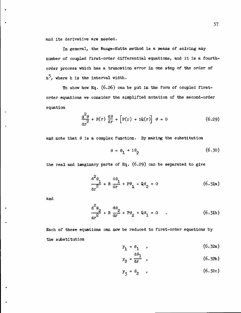
57

and its derivative are needed.

In general, the Runge-Kutta method is a means of solving any

number of coupled first-order differential equations, and it is a fourth-

order process which has a truncation error in one step of the order of

h , where h is the interval width.

To show how Eq. (6.26) can be put in the form of coupled first-

order equations we consider the simplified notation of the second-order

equation

+R(r) H +[p(r) +iQ(r)] 9=0 (6.29)d29 „,_x d9dr2

and note that 9 is a complex function. By making the substitution

9= 9± + 192 (6.30)

the real and imaginary parts of Eq. (6.29) can be separated to give

d29 d9—2^ +R™ +P9X -Q92 =0 (6.31a)dr

and

d29 d9—-f- +R—£ +P92 +Q9X =0 . (6.31b)dr

Each of these equations can now be reduced to first-order equations by

the substitution

yx = 9± , (6.32a)d91

yg=£r , (6.32b)

y, - e2 , (6.32c)

58

d<92yk'sr > (6-32d)

so that Eqs. (6.31a) and (6.31b) become the set of four coupled equations:

dy^ - y2 =0 , (6.33a)

dyp£-£ +Ry2 +Tyx - Qy? =0 , (6.33b)

tilaT " J4—• - y. = 0 > (6.33c)

ayj,5J- + Ryu + Py5 +Qyx = 0 . (6.33d)

Hence, each solution of Eq. (6.26) involves the solution of four coupled

first-order equations, which is also true of Eq. (6.20).

To start the integration from r = 0, the conditions given in

Eq. (6.27) and (6.28) are used:

yx(o) =D , (6.34a)

72(0) =0 , (6.34b)

y5(o) =D , (6.34c)

\(0) =0 , (6.34d)

where D is an arbitrary real constant.

E. Determination of the Normalizing Constant and Complex phase Shift

The function resulting from the integration of the radial differ

ential equation is not normalized properly as a result of the arbitrary

59

constant used in the starting conditions. This means that a numerically

determined radial function will differ from the required asymptotic

forms given in Eqs. (5-10) or (5.11) by a complex constant which must be

determined. To obtain the constant without integrating to very large

values of r, the radial differential equation is written as

X* +p2(r)X =0 ; (6.35)

2for r greater than the nuclear radius, p is real, and for r suffic-

p

iently large, p is positive as well as real. In the latter case the

W.K.B. approximation 0 for the solution to Eq. (6.35) is

1/29£^0 =

LicM.sin /'K(r) dr + t\ (6.36)

where K(r) is a function approximated by p(r), tj is the complex phase

shift, and the asymptotic form of % and 0 is given by

X =0~ sin [G(r) + rf\ . (6.37)

In Eq. (6.37), the function G(r) has the form appearing in Eq. (5«10) or

(5.11).

The approximation X^ 0 in Eq. (6.36) can be achieved to a higher

degree of accuracy for intermediate values of r if a better approximation

than p(r) for the function K(r) is used. The better approximation for

K(r) can be obtained by noting that 0 satisfies the differential

equation

'"♦[^♦ir-Kf1)2]'-0 (6-38)and that for 0 to be also a solution to Eq. (6.35),

p -X- +— -jj-.x2

(¥) (6.39)

6o

Now, if p is slowly varying with respect to r, the iteration

and then obtaining

9

K" /K'\

with the starting condition that Kg = p, will converge very rapidly. In

fact, it is satisfactory to carry the iteration only one step, which

results in

K=,P2-2̂p

and therefore making 0 a very good approximation to %.

For intermediate values of r the functions 9 and 9' resulting

from the integration of Eq. (6.35) differ from % and %' respectively

by a complex constant, A, which can be determined from Eq. (6.36) by

first setting

9 = A( 7 J sin / /Kdr + 77 ] (6.42a)

i+ifrf > (6A1>

(irw>

' =A(kK)1/2 coa/Atar +Tjj - | |̂ - 9 . (6.42b)From these two equations we can write

B=Jx +iJ2 =I|j 9=Asin//Kdr +a+ic-l , (6.43a)

9' K'9 // c\C s I, + ilp = r-7_- + =-75 = A cos//Kdr +a + id , (6.43b)(mo / 2K(kK)v y y

where the complex phase shift is written as 77 = a + iS. By summing the

squares of Eqs. (6.43a) and (6.43b),

A2 =(j^ -J2 +I2 -I2^ +i(2JxJ2 +21^)=Nx +iN2 , (6.44)

which leads to

and finally to

A =

lAl2 . /^ ♦ ^

lAl2 + N N•z + i

N2|

|A| 2 - N

6l

(6.1.5)

(6.46)

which gives the normalizing constant.

The imaginary part of the complex phase shift can now be easily

obtained in the form of e" , which is the form required in F(£ / / L),

by using Eqs. (6.43a) and (6.43b) to write

( /Kdr +a+i5) -icos f/Kdr +a+io

= (J± + I2) + i(J2 -Ij , (6.47a)

sin [ /Kdr +a - iS )+i cos ( /Rdr +a - ib J =

= (J± +I2) -i(J2 -Ix) . (6.47b)

B - iC = A sin

B* + iC* = A*

By multiplying these two equations together,

2 -28(J± +I2)2 +(Jg -Ix) =lAl2 [cos(2i6) +isin(2i5)] =|A| e

which gives the desired term as

-S (J1 +^ + (J2 " Il)

(6.48)

(6.49)

where |A| is given in Eq. (6.45).

In practice, the solutions to the radial differential equations

were terminated when the value of A obtained from Eq. (6.46) converged

to a constant value, indicating that the approximation for X given in

62

Eq. (6.36) was sufficiently accurate.

F. Performing the Integration in F(£.£2£-X)

The integral in the function F(£.£2£jJ) is of considerable

interest from the standpoint of obtaining the matrix elements for pro

cesses involving only continuum wave functions. From a numerical point

of view little has been done to develop methods of obtaining the infinite

integrals of slowly converging oscillating functions, and little has been

published on this subject.

The problem is to find an integral of the form

£T=llmlt / f(x) dx =lifflit I(r) , (6.50)r-»-oo 1^ r-^co v '

where f(x) is a slowly converging function which oscillates about zero,

by solving for l(r) and deducing its limiting value. Since f(x) oscil

lates about zero and converges to zero, the function l(r) for large r

will oscillate about some mean value and converge to that value. The

first approach then is to integrate to some value r for which the magni

tude of the oscillations of l(r) is small compared with the mean value.

However, in the present problem this value was prohibitively large. This

means that for economy, the asymptotic value of the integral must be

determined in the range where the oscillations of l(r) are a significant

fraction of the mean value. Coupled with the fact that l(r) may not be

very regular in its oscillations about the asymptotic value, this value

is very difficult to derive with any degree of accuracy. Additional

methods of smoothing out the oscillations by taking the average value of

63

l(r) as shown by Titchmarslr still result in an oscillating function

I(r) which converges to a limit in a not too regular way. Therefore,

still another method must be devised.

The method devised for solving the integrals was to put a con-

-QJXvergence factor in the integrand of the form e . Then, for selected

values of a, the integral

T(a, r) =/ e_ax f(x) dx (6.51)^0

will converge quite rapidly to the value of the integral

T(a) = / e_ax f(x) dx . (6.52a)(a) =rJo

To find the value of T(o), which is the required value, the value

of the integral T(a.) is found at n + 1 values of a±, i = 1,2,..., n + 1,

and extrapolated to a =0, the method of extrapolation depending on the

function T(a). A convenient method of extrapolation is to fit an nth-

order polynomial to the values T(a ) and solve for a = 0. This can be

1° ,done with the aid of the Lagrange formula

n+1

T(0) = 2^A- T(a-) ' (6.52b)i=l

where the constants A are given by

i-1 a, n+1 a

Ai - IT whn TT vrhn • (6-52°)j=l K A i k=i+l v k i'

%. C. Titchmarsh, Introduction to the Theory of Fourier Integrals(Oxford University Press, London, 1948), 2nd ed., p. 26.

l0W. E. Milne, Numerical Calculus (Princeton University Press,Princeton, 1949), P- 8~3^

64

The convenience of Eqs. (6.52) is made very clear when the a. are equally-a-ix

spaced and we let y = e , where a, is the smallest value of a . In

this case, it is found that

T(0) =/ 2L Ay1 f(x) dx . (6.53)Jo i=l

The sacrifice of calculating the exponential and polynomial in the

weighting factor of Eq. (6.53) at each step of the integration is more

than compensated for by the rapid convergence of the integral and the

resulting time saved in computing f(x). An even greater advantage is

that T(a) is usually a slowly varying function of a and may be monotonic,

which means that it can easily be extrapolated to zero, and such was not

the case in the original problem. The slowly varying nature of T(a) can

be observed from the following two examples:

-ax sinx ,.-11 ., .e —— dx = tan - , (6.54)

0 a

and

oo—ax 1

e sinx dx = — . (6.55)0 a + 1

IV. THE GENERAL PLAN OF THE CALCULATION

Because of the duplication of functions that appear in the terms

of the sum in the function K given in Eq. (5.51), the most economical

method of solution was to carry forward the integration of the differ

ential equations for all the required radial functions one step at a

time. At the end of each step the values for the functions and the

values of the spherical Bessel functions at that step were distributed

65

into the integrations appearing in all the functions F(-£,iL^,L), and

these integrations were carried forward one step. Returning to the

radial equations, the step-by-step process was continued until the

functions F(£••,£2^A>) converged and all the normalizing constants and

phase shifts for the radial equations were obtained. The functions

F(£,£~£jL) were then renormalized and multiplied by the exponential of

the phase shifts, and the final sum in the function K was performed.

The value of K obtained in this way was then used in the cross-section

formula Eq. (6.1).

The actual calculation was complicated by the complex nature of

the functions. In order to obtain each radial equation four coupled

first-order differential equations had to be integrated, and in order to

find each integral in the functions F(££_£.L) a real and imaginary

integral had to be obtained. These complications were intensified by

the necessity for economy and space limitations in the computer which

made it mandatory that no extra integrals be found even though the

allowed values of £ , £', £ , and L did not index in a regular way. The

solution to the indexing problem was found in a special routine which

controlled storage and the distribution of the wave functions among the

integrals in the process of integration. In effect, it acted as a

speedometer which would produce only allowed combinations of the quantum

numbers in a given sequence that covered all possibilities.

In the sum in the function K the two quantum numbers t. and £,-,

were allowed to be unrestricted and all other quantum numbers were then

restricted by the Clebsch-Gordon coefficients and the Racah coefficients.

In order to cut off the sums at maximum values of £^ and & for the1 3

66

cases where the optical potential was present, it was assumed that pro

duction of pions takes place mainly within the bounds of the potential.

Under these circumstances, the maximum value of these numbers should be

such that the first maximum of the corresponding radial equations lies

just outside the bounds of the potential. This means that

^(Max) Wk2 + = - 2uP -V2 - P2 +£-|- ) (6.54)

and

/ 2% m 2 2N1/2^(Max) »f k2 -—t 2^P - V2 - P2 +L«_ j , (6.55)

where r is the radius of the nuclear potential (1.4 A ' ^ x 10" cm).

This turned out to be a very effective means for choosing the maximum

values. The same method also worked for those cases where the nuclear

potential was neglected but the modified Coulomb potential was retained;

however, the radius, rg, in this case was approximately two and one half

times that indicated above.

As an example, consider a case where the incident photon energy

was 310 Mev, the excess kinetic energy was equally distributed between

the pair of pions, the nucleus was lead, and the nuclear potential was

included. The maximum values of /. and £, were then chosen to be1 3

5 and 3, respectively, based on Eqs. (6.54) and (6.55), and the calcu

lation involved the integration of forty first-order differential equa

tions and the evaluation of 192 integrals. The running time on the

IBM-704 was 20 minutes per case.

67

CHAPTER VII

RESULTS

Calculations of the differential cross section for the electromag

netic production of pion pairs were performed, with exact wave functions

used to determine the effects of the distributed nuclear charge and the

nuclear optical potential. The equations were first solved with the

optical potential neglected and the results compared with the Born

approximation, and, finally, both the modified Coulomb and nuclear poten

tial were included in the computation. The results of these calculations

and the comparisons are presented in this chapter.

I. CALCULATIONS WITH THE COULOMB POTENTIAL

A. The Born Approximation

In Chapter I attention was called to the fact that if the Hamil

tonian included a Coulomb potential which is sufficiently broad and with

magnitude greater than the rest mass of the pion it could not be brought

to diagonal form and led to complex eigenvalues. This is not the case

when the Coulomb potential is included in the perturbation—the resulting

Hamiltonian can be diagonalized, and leads to the Born approximation.

Then the resulting cross-section formula can be investigated without

concern about the magnitude of the Coulomb potential. This point is

made because there is some interest in investigating the effect on the

value of the cross section as one goes from a point charge nucleus to a

In this section the equations will be given in ordinary units,where P is the momentum and E is the energy.

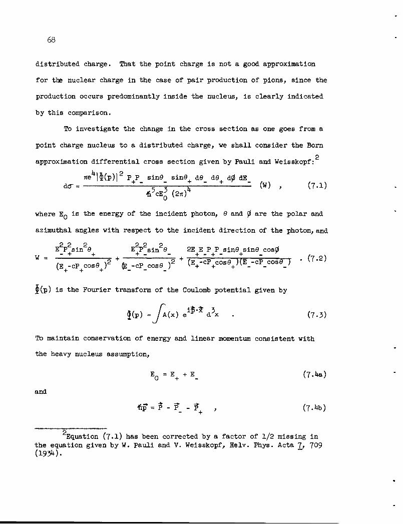
68

distributed charge. That the point charge is not a good approximation

for the nuclear charge in the case of pair production of pions, since the

production occurs predominantly inside the nucleus, is clearly indicated

by this comparison.

To investigate the change in the cross section as one goes from a

point charge nucleus to a distributed charge, we shall consider the Born

2approximation differential cross section given by Pauli and Weisskopf:

ite |$(p)|2 P P sin9 sin9 d9 d9 d0 dEdcr= *" " J - (W) , (7.1)

*5cE^ (2itf

where EQ is the energy of the incident photon, 9 and 0 are the polar and

azimuthal angles with respect to the incident direction of the photon, and

EP sin29 E2p2sin29 2E EPP sin9 sin9 cos0u - - + + + - + - + - + - y /„ _x

/„ ^ a \2 + fr, t, 0 \2 + (E -cP cos9 ME -cP cos9 ) ' K('d>(E -cP cos9 ) (e -cP_cos9 ) v + +*-<•«»<*+/\ _ _/

f(p) is the Fourier transform of the Coulomb potential given by

J(p) =yi(x) e1^'^ d5x . (7.3)To maintain conservation of energy and linear momentum consistent with

the heavy nucleus assumption,

Eg =E+ + E_ (7.4a)

and

*p*=P*-P_-P+ , (7.4b)

Equation (7«l) has been corrected by a factor of 1/2 missing inthe equation given by W. Pauli and V. Weisskopf, Helv. Phys. Acta 7, 709

(1934).

69

where fip* is the momentum transmitted to the nucleus and P is the momentum

of the photon.

For a point charge Eq. (7«3) gives

ftp) =4jteZ

2 '

in which case Eq. (7.1) can be integrated over all angles. After a

tedious calculation, it is found that

2 4 D2 E+Ed<T=OZ--R^IF^ L - 1 dE

(7.5)

(7.6a)

where a is the fine structure constant, R is the classical meson radius,

and

L = logc

2 4PcPc+EE +mc

+ - + -

2~~4"-p cP_c + E E + m c

= 21og„

2 4PcPc+EE +mc

+ - + -

2Enmc(7.6b)

For the case of a distributed charge with density lf(x), Eq. (7-3)

can be shown to lead to

ftp) =-*f j p(x) a1*'* d5x , (7-7)

and Eq. (7.1) has to be integrated numerically.

Equation (7-1) was solved for lead (Z = 82), with the distributed

charge density given in Eq. (2.7) used, and compared with a point charge

lead nucleus. This comparison is given in Figure 3 at a photon energy

of 310 Mev. The two curves have similar shapes, but the point-charge

3 4cross section is a factor of approximately 5 x 10v to 10 larger than

that for the distrubuted charge. This large factor persists in the range

of photon energies investigated in this calculation (280 to 310 Mev).

70

o

>

T3\

bTO

CVJ

8

OUJco

(/)

ooro

UJ

crUJ

u.

o

10

8

0

UNCLASSIFIED

ORNL-LR-DWG 57532

0 0.2 0.4 0.6

FRACTIONAL KINETIC ENERGY, v =2mc2

Figure 3. Comparison of the Born Approximation Pion PairProduction Cross Section at a Photon Energy of 310 Mev fora Point-Charge and Distributed-Charge Lead Nucleus.

71

B. Comparison of Born Approximation and Calculations with Exact Waves

A comparison of the calculation of the pion pair production cross

section using exact waves with the Born approximation solution for a

distributed charge nucleus is presented in Figures 4, 5, and 6. At the

photon energies of 290, 300, and 310 Mev a striking difference in the

spectral shapes between the Born approximation and exact wave calculation

will be noticed. The enhancement of the cross section for higher energy

n+ mesons is well known and occurs because of the repulsive Coulomb

3potential.

The difference between the Born approximation and exact wave

calculations can be expected in the cases just cited because the condi

tions for the Born approximation to hold are certainly not obtained:

rife- - rife- « i • (7-8)+ ' + - ' -

2 2In fact, for lead, where Z=82, EQ =310 Mev, and (E_ -Mc )/(EQ -2mc )=

0.5, then Zcffl/Pc =1.4. It is of some interest then to examine the

spectral shape of the exact wave cross section to see how it approaches

that of the Born approximation as Z->-0. Figure 7 shows the ratio of the

differential cross section for the exact wave solution to that of the

Born approximation as a function of Z for v = 0.5 and 0.1 at photon

energy 290 Mev. In this comparison the value of A, which determines the

A discussion of this point is given for electron pair productionby H. Heitler, The Quantum Theory of Radiation (Oxford University Press,London, 195*4 3rd ed., p. 259-

72

O

>

•o

b

C\J

CE

oUJCO

COCOooro

3.0

2.5

2.0

1.5

UNCLASSIFIED

ORNL-LR- DWG 52733

^ 1.0

LJCEUJ

U.

Q 0.5

0

0 0.2 0.4 0.6

FRACTIONAL KINETIC ENERGY, v =

0.8 1.0

E_— mc2

E0-2mc2

Figure 4. Comparison of the Born Approximation and Exact WavePion Pair Production Cross Section for Lead at a Photon

Energy of 290 Mev. The Nuclear Potential Was Neglected.

o

>

T3

\

b•o

OJ

CEa

oUJCO

COCO

oCEu

UJ

CEUJ

u.u.

Q

3.0

2.5

2.0

1.5

1.0

0.5

0

UNCLASSIFIED

ORNL-LR-DWG 52734

—V^-EXACT WA\ /t~<^/Lb

SUBORN APPROXI MATION

0 0.2 0.4 0.6 0.8 1.0

FRACTIONAL KINETIC ENERGY, v =E_— mc'

E0 - 2mc2

73



74

o

>

bXJ

OJ

CEO

oUJCO

COCOoCEo

UJCE

14

12

10

8

0

UNCLASSIFIED

ORNL-LR-DWG 52735

\ r y££T WAVE o

\^"^ O

r^-BORN

/ APPROXIMAT1

ION

0 0.2 0.4 0.6

FRACTIONAL KINETIC ENERGY, v =

0.8 1.0

E_— mc2

E0-2mc2



<X

UJ

>

\

b

2.0

1.5

2CCo

-> 1.0

bT3

UNCLASSIFIED

0RNL-LR- DWG 52736

0.5

E -v =

EQ"

- mc2

2mc2

\ V -- U. l

n ^\ ^ U. D

0 20 40 60 80

NUCLEAR CHARGE, Z

100

75

Figure 7. Ratio of Exact Wave to Born Approximation DifferentialCross Section as a Function of Z For Photon Energy of 290 Mev.

76

extent of the charge distribution, was kept constant; so the numbers

refer to fictitious nuclei for Z< 82. Referring back to Figure 4 and

2assuming that a Z factor has been removed from the ordinate to make

the Born approximation independent of charge, as Z decreases the exact

wave curve increases steadily relative to the Born approximation, main

taining its shape until Z = 20; for small v it starts to decrease, while

for large v it continues to increase until Z = 0 where the curve has

assumed the Born approximation shape.

The ratio of the total pair production cross section obtained by

exact waves and distributed charge to that obtained by Born approximation

can be determined after integrating the curves shown in Figures 4, 5,

and 6. This ratio is shown in Figure 8. The most interesting fact to

be observed from these data is that the ratio is less than 1 as the

photon energy increases above threshold, reaching and crossing the value

1 at approximately 317 Mev. This is the opposite behavior from that

obtained in electron pair production with a point charge where the ratio

is greater than 1 just above threshold and decreases and finally crosses

the value 1 as the photon energy increases.

II. CALCULATIONS WITH A MODIFIED COULOMB AND NUCLEAR POTENTIAL

In order to select the nuclear optical potential parameters for

the present calculation from the data shown in Figures 1 and 2, it is

necessary to briefly review the way that the data were obtained.

5A discussion of this point for electron pair production is given

by I. E. Dayton, Phys. Rev. 89, 544 (1953).

o<XUJ

b

cr

om

b

.0

0.8

0.6

0.4

0.2

0

UNCLASSIFIED

ORNL- LR- DWG 52737

7/

/

/

270 280 290 300 310

PHOTON ENERGY (Mev)

320

77

Figure 8. Ratio of Exact Wave to Born Approximation Pion PairProduction Cross Section for Lead as a Function of Energy.The Nuclear Potential Was Neglected.

78

In the analysis of the pion scattering data from complex nuclei

it has been customary to introduce both the real and imaginary part of

the optical potential as a time component of a four-vector. In contrast

to this, in Chapter III, it was shown that only the imaginary part of

the optical potential should be a time component of a four-vector, the

real part being a world scalar. In effect this means that the data pre

sented in Figures 1 and 2 were obtained by using a radial differential

equation where the factor -266 (P + iV) rather than -2uP - 2±<uJ V [which

was in Eqs. (5-8) and (5-9)] appeared in the operator. This means that

the real part of the potential in Figure 1 should be corrected by a

factor wk/p in order to make it applicable to this calculation. The

imaginary part of the potential need not be corrected.

In the calculations to be described, incident photon energies up

to 310 Mev were considered, and therefore since threshold is at approxi

mately 279 Mev, the optical potential in the range 0-30 Mev pion

kinetic energy was required. From the data given in Figures 1 and 2 and

from the assumption that the potential curves are flat in the lower

energy region as discussed in Chapter II the values of -16 Mev for the

real part of the potential and -5 Mev for the imaginary part of the

potential were selected.

The differential cross sections obtained from the present calcu

lation including both the Coulomb potential from the distributed charge

in the nucleus and the nuclear optical potential are presented in

Figure 9 and in Table I. These data still show the effects of the strong

Coulomb potential, although the cross section has been considerably

2.6

2.4

2.2

2.0

ora

1.8

i-oUJCD

in</)ocr

1.6

1.4

1.2

1.0

± 0.8

0.6

0.4

0.2

0

UNCLASSIFIED

ORNL-LR-DWG 52738

\ "3i()-Mev PHOTON ENERGY

300 Mev

•^^^290 Mev

0 0.2 0.4 0.6 0.8 1.0

FRACTIONAL KINETIC ENERGY, v =mc'

E0-2mc2

Figure 9. The Differential Pion Pair Production Cross Section forLead Including the Coulomb and Nuclear Optical Potential(P = -16 Mev, V= -5 Mev).

79

80

TABLE I

THE PION PAIR PRODUCTION CROSS SECTION IN UNITS OF CtR = 7-762 x 10~55 cm2FOR LEAD, INCLUDING THE COULOMB AND OPTICAL POTENTIAL

(P = -16 Mev, V = -5 Mev)

E - mc Cross section at photon energy of

T ~ 2EQ - 2mc290 1Mev 300 ]Mev 310 Mev

Differential Cross Section,dc/dv

0

oar

0.001 1.06 x 10-1 8.31 x 10-1 2.16

0.125 7.66 X 10-2 7.91 x 10-1 2.38

0.250 ^•59 x 10-2 7.21 X 10-1 2.V7

0.375 1.99 x 10-2 5.79 x 10-1 2.17

0.500 5.57 x 10-5 U.00 x 10-1 1.63

0.625 7.92 x icf* 1.1+1 x 10-1 9.89 x 10"1

0.750 2.73 x 10-5 1.27 x 10-2 2.53 x io"1

0.875 ^•91 x 10-5 2.68 x 10~5

0.95 2.66 x 10"^

Total Cross Section, —pOR

2.49 x 10"2 3.81 x 10"1 I.38

81

increased from the corresponding cases without the optical potential.

The data at photon energy 310 Mev show a hump which can be accounted for

on the basis that within the nuclear well the effective momentum of the

pions is increased whereas the effects of the Coulomb potential are

reduced and therefore the spectrum would be expected to tend toward the

symmetric shape given by the Born approximation. Figure 10 and Table I

present the integration of the differential cross section as a function

of the incident photon energy indicating a sharp increase in the cross

section about 15 Mev above threshold.

82

ora

1.4

UNCLASSIFIED

ORNL-LR-DWG 52739

1.2

1.0

0.8

0.6

0.4

0.2

n

270 280 290 300 310

PHOTON ENERGY(Mev)

320

Figure 10. The Pion Pair Production Cross Section for LeadIncluding the Coulomb and Nuclear Optical Potential(P= -16Mev,V= -5 Mev) as a Function of Photon Energy.

83

CHAPTER VIII

SUMMARY

The Pauli-Weisskopf theory of the electromagnetic production of

pion pairs has been investigated with the objective of including in it

the strong pion-nucleus interaction which ultimately leads to an enhance

ment of the cross section. This was accomplished by the semiphenomenolog-

ical method of including the interaction into the rigorous theory in the

form of an optical model, a method first suggested by landau and

Pomeranchuk.

In Chapter III it was shown that the optical model in the form of

a complex optical potential could be explicitly introduced into the field

equations in a consistent manner which leads to the absorption and

scattering of the pions from the nucleus. The consistency of the theory

is maintained only in the case where the real part of the potential is

a world scalar and the imaginary part a time component of a four-vector.

Absorption of mesons in the nucleus as introduced into the theory

by the imaginary part of the optical potential includes all inelastic

events as well as true absorption which leads to an excited state of the

nucleus. The real part of the potential, on the contrary, introduces the

coherent scattering of the mesons from the nucleus as a whole. The

resulting cross section with these potentials therefore represents the

\. Pauli and V. Weisskopf, Helv. Phys. Acta ]_, 709 (193*0 •

2L. D. Landau and I. I. Pomeranchuk, Zhur. Eksptl. i Teort. Fiz.2k, 505 (1953); English translation: Proceedings of the Cern Symposium1956 (Service d'Information] Cern, 1956), vol. II, p. 159*

81+

pion pair production cross section where the nucleus is left in its

ground state.

When the optical potential is present, the final-state wave forms

for the pion wave functions appearing in the matrix element are not fixed

by existing theory. Therefore a choice between two possible forms had

to be made. It was possible to make the selection unambiguously, however,

as was shown in Chapter IV. The resulting matrix element was then ex

pressed in angular momentum states for ease of solution, and methods of

solution were devised for the various terms. These last two steps are

shown in Chapters V and VI. Of particular interest in Chapter VI is the

method devised for finding certain infinite integrals that appear in the

matrix element, where the integrand is a product of continuum wave

functions or their derivatives. This problem was resolved by the intro

duction of a weighting factor in the integrand which made the integral

converge quite rapidly.

Since the production of pion pairs occurs predominantly inside

the nucleus, it was necessary to consider the modified Coulomb potential

resulting from a finite nucleus with a distributed charge density. The

form of the charge density used was that obtained from electron scat

tering experiments. The complication of the distributed charge has its

compensation in that now the ambiguity occurring in the equations of

motion for JL = 0 is avoided, as are the complex eigenvalues that could

arise if the Coulomb potential is sufficiently broad and has too large

a magnitude.

The results of the calculations for photon energies just above

threshold shown in Chapter VII indicate a considerable change in the

85

spectral shape of the differential cross section when exact waves are

used as compared with the Born approximation results. The enhancement

of the cross section for it mesons with energy greater than the it" meson

is very evident and can be attributed to the repulsive Coulomb potential

for the it mesons. Although the cross section is markedly reduced as

one goes from a point charge to a distributed charge for the nucleus,

the loss is regained when the strong pion-nucleus interaction is included

in the form of the optical potential. Tnis increase in the cross section

is significant, putting the values in an experimentally determinable

region especially for photon energies above 295 Mev.

It was pointed out in Chapter I that the it-it interaction was

neglected in this calculation. This was done because at the present

time there is insufficient information available for an adequate treat

ment of the interaction.

In the present state of affairs, it is difficult to speculate as

to the effect of the it-it interaction on the spectral distribution of the

pion pairs, or, for that matter, on the cross section for the production

process. Only a few qualitative statements can be made.

First, it should be pointed out that at gamma-ray energies just

above threshold such as those considered in this paper, the maximum

center-of-mass energy of the pion pair is relatively low (approximately

2.2 ji). This is well below the start of the proposed resonance in the

isotopic spin t = 1 state of the it-it system which is located at an energy

^ kof approximately k u. ' It would also be below the t = 0 resonance

\. R. Frazer and J. R. Fulco, Phys. Rev. Letters 2, 365 (1959).

P. Curruthers and H. A. Bethe, Phys. Rev. Letters k, 536 (i960).

86

ksuggested by Curruthers and Bethe which, if the resonance actually

exists, would be located at an approximate energy of 2.5 u. For these

reasons, serious fluctuations from the cross section as calculated in

this paper should not be expected.

kIt was pointed out by Curruthers and Bethe that the t = 0 inter

action might be expected to dominate at the lower center-of-mass energies

of the n-jt system. Rodberg has reported some impulse approximation

calculations of the it~ + p -*•« + it" + n reaction which seem to sub

stantiate this. In the lower energy range he assumed the dominance of

the t = 0 interaction and obtained reasonable agreement with the experi

mental results of Perkins et al. Assuming that the t = 0 interaction

is dominant at low center-of-mass energies of the n-n system and noting

that the n -«" pair is a mixture to t = 0, 1, and 2, the interaction

might well affect the results presented in this paper and be observable

by comparison with experimental data.

Although the present calculations maintained at least 1$ numerical

accuracy, a much larger error no doubt occurred because of the uncertainty

in the optical potential parameters selected from the spread of experi

mental data. A systematic study of the effect of changing the values

of the potential parameters and shape would give an indication of how

sensitive the present results are to these factors. However, an improve

ment in the analysis of the experimental data and more values from the

5L. S. Rodberg, Phys. Rev. Letters 3, 58 (1959).

Perkins et al., Phys. Rev. Letters 3, 56 (1959).

87

low-energy pion-nucleus scattering experiments would ultimately be

necessary to improve the values of the potential parameters and lead to

a more accurately calculated pion pair production cross section. An

improved analysis of the scattering data would result if the radial

equations of the form given in Eqs. (5.8) and (5.9)> which includes the

effects of the modified Coulomb potential, were used.

89

BIBLIOGRAPHY

Baker, Rainwater, and Williams, Phys. Rev. 112, I763 (1958).

Bethe, H. A., Phys. Rev. 57, 1125 (19^0).

Bethe, H. A., and F. de Hoffmann, Mesons and Fields (Row, Peterson andCompany, Evanston, 1955)> vol. II.

Bethe, H. A., and W. Heitler, Proc. Roy. Soc. (London) A1^6, 83 (193*0•

Bethe, H. A., and R. R. Wilson, Phys. Rev. 83, 690 (1951).

Biedenharn, L. C, Tables of the Racah Coefficients, USAEC ReportORNL-IO98, Oak Ridge National Laboratory (1952).

Breit, G., and H. A. Bethe, Phys. Rev. 93, 888 (195*0.

Byfield, Kessler, and Lederman, Phys. Rev. 86, 17 (1952).

Condon, E. U., and G. H. Shortley, Theory of Atomic Spectra (CambridgeUniversity Press, Cambridge, 1935).

Curruthers, P., and H. A. Bethe, Phys. Rev. Letters *+, 536 (i960).

Dayton, I. E., Phys. Rev. 89, $kk (1953).

Fernbach, Serber, and Taylor, Phys. Rev. 7£, 1352 (19*^9)•

Frank, Gammel, and Watson, Phys. Rev. 101, 89I (1956).

Francis, N. C, and K. M. Watson, Phys. Rev. 92, 291 (1953).

Frazer, W. R., and J. R. Fulco, Phys. Rev. Letters 2, 365 (1959).

Gill, S., Proc. Cambridge Phil. Soc. 1+7, 96 (1951)-

Goldstein, H., Classical Mechanics (Addison-Wesley Publishing Company,Inc., Cambridge, 1953).

Heitler, W., Quantum Theory of Radiation (Oxford University Press,London, 195*0-

Hofstadter, R., Revs. Mod. Phys. 28, 211+ (1956).

Kisslinger, L. S., Phys. Rev. 98, 76l (1955).

Landau, L. D., and E. M. Lifshitz, Quantum Mechanics (Addison-WesleyPublishing Company, Inc., Reading, 1958).

90

Landau, L. D., and Iu. la. Pomeranchuk, Zhur. Eksptl. i Teort. Fiz. 2k,505 (1953); English translation: Proceedings of the Cern Symposium1956 (Service d*Information, Dern, 1956), vol. II, p. 159-

Lattes, Occhialini, and Powell, Nature l60, 1+53 (l9*+7).

Milne, W. E., Numerical Calculus (Princeton University Press, Princeton,19U9).

Mott, N. F., and H. S. W. Massey, The Theory of Atomic Collisions(Oxford University Press, London, 19*+0).

Pauli, W., and V. Weisskopf, Helv. Phys. Acta J_, 709 (193*+).

Perkins et al., Phys. Rev. Letters 3, 56 (1959).

Pevsner, et al., Phys. Rev. 100, 11+19 (1955).

Pomeranchuk, Iu. la., Dokl. Acad. Nauk SSSR, 96, 265 and l+8l (195*+);English translation: Proceedings of the Cern Symposium 1956(Service d'Information, Cern, 1956), vol. II, "p. I67.

Racah, G., Phys. Rev. 62, I+38 (l9*+2).

Racah, G., Phys. Rev. 63, 367 (19**3).

Rodberg, L. S., Phys. Rev. Letters % 58 (1959).

Rose, M. E., Elementary Theory of Angular Momentum (John Wiley and Sons,Inc., New York, 1957).

Rose, M. E., Multipole Fields (John Wiley and Sons, Inc., New York, 1955).

Saphir, G., Phys. Rev. 101+, 535 (1956).

Sapiro, A. M., Phys. Rev. 8J+, IO63 (1951).

Schiff, Snyder, and Weinberg, Phys. Rev. 5J, 315 (I9I+O).

Schiff, L. I., Quantum Mechanics (McGraw-Hill Book Company, Inc.,New York, 1955T

Schweber, Bethe, and de Hoffmann, Mesons and Fields (Row, Peterson andCompany, Evanston, 1955), vol. I.

Simon, Vander Sluis, and Biedenharn, Tables of the Racah Coefficients,USAEC Report ORNL-I679, Oak Ridge National Laboratory (195*+).

Simon, A., Numerical Tables of the Clebsch-Gordon Coefficients, USAECReport ORNL-1718, Oak Ridge National Laboratory (195I+).

91

Snyder, H., and J. Weinberg, Phys. Rev. <?]_, 307 (l9*+0).

Stork, D. H., Phys. Rev. 93, 868 (195*0-

Takeda, G., and K. M. Watson, Phys. Rev. 97, 1336 (1955).

Titchmarsh, F. C, Introduction to the Theory of Fourier Integrals (OxfordUniversity Press, London, ISkH), 2nd ed.

Vdovin, Yu. A., Doklady Akad. Nauk S. S. S. R. 105, 9*^7 (1955).

Watson, K. M., Phys. Rev. 105, I388 (1957).

Watson, K. M., Phys. Rev. 89, 575 (1953).

93

APPENDIX A

REDUCTION OF THE FIRST-ORDER PERTURBATION THEORY MATRIX EIEMENT

WITH EXACT WAVES TO THAT OBTAINED WITH SECOND-ORDER

PERTURBATION THEORY WITH PLANE WAVES

It will be shown here that the matrix element

Yo) d5r (A.l)M = -2ie *K(given in Eq. (5-5)] obtained from a first-order perturbation theory

treatment of the interaction between the meson and electromagnetic

field using exact waves reduces to the results obtained by Pauli and

Weisskopf in a second-order perturbation theory treatment using plane

waves if the Born approximation is made. In order to simplify the

derivation and make it directly comparable with the results of Pauli

and Weisskopf, the nuclear optical potential will be set to zero in the

differential equations for the wave functions. Then, from Eqs. (k.2)

and (*+.3),

(-V2 -kf) yt =(2^ eAQ -eSAS0) Y^j »l^ , (A.2)

+ + + +

where

CJ2 =k2 + u2 . (A.U)

9i+

The waves in Eqs. (A.2) and (A.3) have the following asymptotic forms

ikr

ikr

C+ + r/2%where the notations

ijt-r

(A.7)"it

0e - ^—- (A.8)^\

have been used. Equation (A.2) can now be written in operator form as

V Y+~r+ . 0* +—--J^L- , (A.9)'*- *- HQ -k_ -i£

where H = - \/ , 6 is a real infinitesimal constant which approaches

.*zero, and y+ is the solution to the homogeneous equation. To get a

more explicit form for Eq. (A.9), it can be written as

- - J H (r) -k2 . i£

and

Z ^ 4(?,) v*=S(?-?,) * (A-n)

where the waves are assumed to be quantized in a box of unit volume.

95

Using Eq. (A.11) in Eq. (A.10),

2^0g(?)(0rV_Y^)Y% (?) -I (?) +A, ^ g2 1 - "K- , (A.12)

"k- ^ k* k1" - k^ - i£

where

(%' V-^ )=f0lY-^ ^ ' (A'15)Similarly, the expression

*±<teM(H»\X)*+ + ^=V kf - k - it

k'

can be obtained.

For the potential A*,

where unrationalized units are used and e is a unit vector in theq

direction of polarization. This wave is transverse, so that e *q* = 0.

Inserting Eqs. (A.12), (A.l*+), and (A.l6) into Eq. (A.l) yields

i(<MV£>r- 3

i(3-V^'7A w \ 5Ar—» Hdl e

«£-*£ -i«0(A.16)

^r— itf+it'-tj.? *. 5second-

order

term.

96

In Eq. (A.16) the second-order term contains a factor V V and

2therefore is of order e , but it is dropped subsequently, since only

terms of order e are retained. The first term on the right of Eq. (A.l6)

can also be dropped because it leads to the Dirac delta function

&(q* -£-]?), which will give no contribution because the theory

requires that co» = cz + cj and both conditions cannot be satisfied.

Before substituting the values of V+ and V in the remaining

terms of Eq. (A.l6) the terms of order e are dropped, and the Fourier

transform is introduced:

where

AQ(r) ,y>^? U$) , (A.17)

ftp) =J eif**AQ(r) d5r , (A.18)so that

and

V+ =-2^ e\ e-ipV?|(p) (A.19)

V_ =2^ e\ e"ip**? |(p) . (A.20)

Now, the Born approximation

Yi -* £ (A.21)

Yj* •* 4 (A-22)

is introduced and Eqs. (A.19) and (A.20) are used to obtain

and

= td e

k

(*"V+^)-%

-i(p+l+tj-r ,e $(p) d^i

^k^_

&($ + \ + £ )$(P)

^(f +lt+ k*+)$(p)

J^\Equation (A.l6) now becomes in the Born approximation

M = 2e <Jkit2 2

97

(A.23)

(A.21+)

(A.25)

(8 -t_)<u S(t +t' -t_) S>(J +*• +£+)

¥• ? /^vv *£ "-2.

where 6 is set equal to zero. The sums in Eq. (A.25) can now be per

formed, and the condition e-q" = 0 used to obtain

2 /*+*_2W_

M = 2e

with

^fZZT (e_ 'k )

^\ 1

«-4+<)V^ (^-4-j)^.-i(p) >

(A.26)

P* = q -k_ -k+ , (A.27)

which is the form of the matrix element from the Pauli-Weisskopf theory.

98

APPENDIX B

A LIST OF SOME USEFUL RELATIONS BETWEEN CIEBSCH-GORDON

AND RACAH COEFFICIENTS

For the purposes of reference, a few equations involving the

Clebsch-Gordon and Racah coefficients are reproduced in this Appendix.

These equations are contained in the book by Rose, along with others

that are of considerable interest but not explicitly referred to in

this work.

Four useful symmetry relations of the Clebsch-Gordon coefficients

2are

C(j1j2jym1ni2in5) =(-1) ° cO^jy -ny -mg, -m^ , (B.l)

Jt+Jo-J*;= (-1) d ° C(j2j1jym2m1m5) , (B.2)

J1-ID1 l2h +X\1/2= (-1) f2jTTJ C(j1J3J2;m1,-m5,-m2) , (B.3)

J2+m2 /2j +1\V2=(-X) (2j7TtJ C(j5j2j1;-m3,m2,-m1) , (B.1+)

M. E. Rose, Elementary Theory of Angular Momentum (John Wileyand Sons, Inc., New York, 1957).

2Ibid., p. 38.

99

and two equations relating the Racah and Clebsch-Gordon coefficients

3are

^ [(2e +l)(2f +l)]1/2 W(abcd;ef) C(bdf;p6) C(afc;a,p +o)f

= C(abe;ap) C(edc;a + P, o) ,

[(2e +l)(2f +l)]1'2 W(abcd;ef) C(afc;a, P+&)

•? C(abe;ap) C(edc;a + p, S) C(bdf;p6)

^Ibid., p. 110. A typographical error in the first Clebsch-Gordon coefficient on the right of Eq. (B.6) was corrected beforereproducing the equation here.

(B.5)

(B.6)

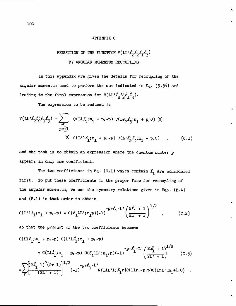
100

APPENDIX C

REDUCTION OF THE FUNCTION VtLL'i^Z-j/)

BY ANGULAR MOMENTUM RECOUPLING

In this appendix are given the details for recoupling of the

angular momentum used to perform the sum indicated in Ey.. (5.36) and

leading to the final expression for V(LL'/£,'££).

The expression to be reduced is

V(LL-/2/^3) =Y] C(LlZL;ml +p,-p) C(L/2i ;m +p,0) Xm-i '

p=+l

X C(LIli1;ra1 +p,-p) C(L'/2^3;m1 +p,0) , (C.l)

and the task is to obtain an expression where the quantum number p

appears in only one coefficient.

The two coefficients in Eq. (C.l) which contain L. are considered

first. To put these coefficients in the proper form for recoupling of

the angular momentum, we use the symmetry relations given in Eqs. (B.1+)

and (B.l) in that order to obtain

-P+/.-L72*1 +1\V2C(L'l£1;m1 +p,-p) =C(i1lL';m1p)(-l) x ^j +1j , (C.2)

so that the product of the two coefficients becomes

CClU^ +p,-p) C(L'li1;m1 +p,-p)

= C(lAl ;m + p,-p) C(£ lL';m.,p)(-l) "* [ —± -1 (C3)-p+^-L'/2^ +lX1/2:(Ll/.1;mi +p,-p) c(^1lL';m1,p)(-l) 1 (^ +J (c.

(2-^+1 )2(2r+l)4r L

1/2 -p+2 -L'(-1) W(LlL'l;/1r)c(llr;-p,p)c(LrL,;m1+l,0) .

(2L« + 1)

101

Equation (B.5) has been used to obtain the last form for the product

given in Eq. (C3)«

After substituting Eq. (C3) into Eq. (C.l) and gathering the

three coefficients containing m,, we consider the sum

y C(LrL*;m1 +p,0) C(L^;m1 +p,0) C(L'^^;m1 +p,0)mlZL+rL' L-m -p/2^+l\

C(rLL';0,m1+p)(-l) C^/^+v, -m1-p)(-l) (gZ+i im, \ 2 /

L'-m^P^^+lX1/2

1/2

C(L'/3i2Jm1+p,-m1-p)(-l) - ^~j (c*0

where the symmetry relations (B.2) have been used on the first coefficient,

and (B.3) on the second and third coefficients. Because of the arrange

ment of the quantum numbers in the coefficients on the right of Eq. (C.*+)

Eq. (B.6) can now be used to obtain

y C(LrL';ml +p,0) C(L/2^;m;L +p,0) CtL'/^n^ +p,0)1/2(2L' + l)(2i + l)2

(24* + i)(-1)1" Z(xi^2,00) W(rLe^;L^2)

Gathering terms, V now becomes

(2£± +I)2 (2r +l)(2# +l)2V(LL Vi&V =l_

p=+l

(2V2 + 1)

(C5)

1/2

(-D Xp+Z.-L'+r

X C(lJj;-p,p) C(r^;00) WfLlLl^r) W(rL^^jL'/2) , (C.6)

and the primary objective of obtaining an expression with the quantum

number p in one coefficient has been achieved.

102

To proceed, use is made of the fact that i_ + £', L + L' and

L' + £ + 1 must be even in the expression for K given in Eq. (5.35).

This was established in the section following Eq. (5.36). With / +/*

even and since r+£>2 +l^ must be even in the coefficient C(r-4-£*;00)

appearing in Eq. (C.6) for non-zero results, the quantum number r must

now be even. This condition and the condition that r must satisfy a

restricted triangle condition in the coefficient C(llr;-p,p) in Eq. (C.6)

leaves r with only two possible values, 0 and 2.

For r = 0,

and for r = 2

C(llO;-p,p) =-2- , (c.7)p=+l V3

C(ll2;-p,p) =y| , (C.8)p=+l

so that

(2/+l)(2£+l)V(LL'i2i-^) - ^)+i)^/2 ^ C(0£/';00) W^L-l^O) W(0Li^;L'/2) +

(21 +1)(2 4.+1) fj7r+ (g^+l)l/2 j/t ^Vs'00* ^(LlL.l;^) W(2L^;L.£2) .(C9)

The coefficients in the first term on the right of Eq. (C9) can be

evaluated to give

0(04^00) - s^, ,6

W(L1L'1; to) = ^^ >^ [3(2L•+!)] V2

U 103

w(0L£2%;L'4) = L'L' ^jL ,23 2 [(2L+l)(2/2+l)]1/2

where use is made of the conditions that I + /', L + L1 and L' + / + 1

are even.

The value of the second term on the right or Eq. (C.9) will be

unaltered by using the symmetry relation (B.1+) on the Clebsch-Gordon

coefficient. Using this relation, the final expression for V becomes

(2Z+1)(2^+1)

VfLL'/^W -j (2^+1)(glil) \,L' %,£' +

+(2^+l)(2/3+l)(-l) 2J| C(^2j00) WdJL'lj/^) X

X W(2L£^3;L^2) , (CIO)

which is the form used for Eq. (5«37).

1.

2.

3.I+-60

7-

8-27-28.

29-30.

31.

32.

33.

3*v.35-36.37-38.39-1+0.

1+1.1+2.

k->.!+*+.

*+5.1+6.

ki.1+8.

1+9-

Co E. Center

Biology LibraryHealth Physics LibraryCentral Research LibraryReactor ExperimentalEngineering Library

Laboratory Records DepartmentLaboratory Records, ORNL R.CA. M. Weinberg

L. B. Emlet (K-25)J. P. Murray (Y-12)J. A. Swartout

G. E. BoydR. A. CharpieW. H. Jordan

A. Ho Snell

C. E. Winters

E. P. Blizard

D. S. BillingtonF. L. Culler

J. Lo Fowler

J. H. Frye, Jr.

C. S. Harrill

A. Hollaender

A. S. Householder

C. P. Keim

Mo To KelleyS. C. LindR. S. Livingston

INTERNAL DISTRIBUTION

ORNL-3033Physics and Mathematics

TID-1+500 (15 ed.)October 21, i960

50, Ko Zo Morgan

510 Mo Lo Nelson

52 0 Ho E. Seagren

•y 53. E 0 D. Shipley

5k 0 Eo Ho Taylor55o Po Mo Reyling

irtment 56. Do Phillips

ILR.Co 57- Mo Jo Skinner

580 R. L. Becker

59- Nancy M. Dismuke600 A. Co Downing

61. M. E. Rose

62. G. R. Satchler

630 T. A. Welton

61+. Go T. Trammel

65-89. Co D. Zerby

90. A. Do Callihan

910 Ho Bertini

92o Lo B. Holland

93. R. E. Maerker

9k. F. C. Maienchein

95 0 Fo J. Muckenthaler

96. A. Simon

97- Wo A. Gibson

98. P. P. Gast (consultant)99. Herbert Goldstein (consultant)

100. L. W. Nordheim (consultant)101. R. F. Taschek (consultant)102. To J. Thompson (consultant)

EXTERNAL DISTRIBUTION

103. P. F. Zweifel, Department of Nuclear Engineering, University of Michigan,Ann Arbor, Michigan

10l+. R. B. Curtis, Department of Physics, Indiana University, Bloomington, Indiana105-71)+. Given distribution as shown in TID-1+500 (15th ed.) under Physics and

Mathematics category (75 copies - 0TS)715. Division of Research and Development, AEC, 0R0

105

contract no. w-7^05-eng-26

Documents