control of oxygen excess ratio in a pem fuel cell system...
TRANSCRIPT

Turk J Elec Eng & Comp Sci
(2015) 23: 255 – 278
c⃝ TUBITAK
doi:10.3906/elk-1301-90
Turkish Journal of Electrical Engineering & Computer Sciences
http :// journa l s . tub i tak .gov . t r/e lektr ik/
Research Article
Control of oxygen excess ratio in a PEM fuel cell system using high-order
sliding-mode controller and observer
Seyed Mehdi RAKHTALA1,∗, Abolfazl Ranjbar NOEI1,Reza GHADERI1, Elio USAI2
1Department of Electrical and Computer Engineering, Babol University of Technology, Babol, Iran2Department of Electrical and Electronic Engineering, University of Cagliari, Cagliari, Italy
Received: 15.01.2013 • Accepted: 08.04.2013 • Published Online: 12.01.2015 • Printed: 09.02.2015
Abstract: The main objective of this manuscript is to design a high-order sliding-mode observer to provide finite time
estimation of unmeasurable states (x4 : oxygen mass, x5 : nitrogen mass) together with the oxygen excess ratio (ratio of
the input oxygen flow to the reacted oxygen flow in the cathode). This is done by applying second-order sliding modes
through either super twisting or suboptimal controllers to control the proton exchange membrane fuel cell’s breathing.
The estimated oxygen excess ratio is controlled in a closed-loop system using 2 distinct sliding-mode approaches: a
cascaded super twisting controller and a single-loop suboptimal structure. Simulation results are presented to make
a quantitative comparison between the cascade and the single-loop configuration. The results verify that the cascade
provides accurate reference tracking while the single-loop presents faster convergence.
Key words: Proton exchange membrane fuel cell, oxygen excess ratio, high-order sliding-mode observer, cascade control,
second-order sliding mode
1. Introduction
A fuel cell is an electrochemical device to convert chemical energy into electrical energy with thermal dissipation
[1]. In comparison with regular power resources, this offers several advantages, such as high efficiency and a
flexible modular structure [2]. However, as a drawback, the reaction time constant is dominated by temperature
and oxygen starvation during rapid load transients [3]. Therefore, the proton exchange membrane fuel cell
(PEMFC) performance is closely related to the type of control system.
Oxygen starvation is a complicated phenomenon that causes a rapid decrease in the cell voltage, which
creates hot spots in severe cases or even burns the surface of the membrane. Pukrushpan et al. [4,5] reported
that acceptable amounts for the oxygen excess ratio (λO2) are within 2–2.4 based on the stack power. Therefore,
it must be regulated around the constant value to cope with the oxygen starvation. This may be fulfilled through
control of the oxygen-providing mechanism, i.e. the compressor PEMFC, to achieve a satisfactory performance.
As a necessary condition, the dynamic response of the compressor motor controller has to be fast.
Recently, several control strategies were proposed for PEMFC systems. Among them, feedback lineariza-
tion [6–8], feed forward control [5,9], sliding-mode control [10], and the super twisting algorithm with and
without feedforward control [11,12] are such important and efficient techniques. Although an air mass flow
sensor may be used to assess the oxygen excess ratio, it ruins the performance. This is because its time re-
∗Correspondence: mhj [email protected]
255
RAKHTALA et al./Turk J Elec Eng & Comp Sci
sponse is about 1–2 s, which produces a long delay in the controller. The most common interest in [11–13] was
using the airflow sensor specifically in a real-time application. However, sensor-based control has the following
shortcomings:
• Slow response time (1–2 s),
• Short life time (6 months to 3 years),
• Less accuracy (1%–10%),
• Price (US$1000),
• Inevitable instrumental noise.
These restrictions are also applicable when the oxygen excess ratio is controlled through an inlet oxygen
flow in the cathode (WO2,in) measurement. Therefore, a sensorless approach is of interest in the current work.
Talj et al. [14], in 2009, used a cascade structure for a PEMFC. Although their work had the advantages of a
high-order sliding-mode (HOSM) controller, it again faced the following restrictions:
1. Sensor-based scheme has the above-mentioned drawbacks.
2. Instrumentation lag occurs in the overall system dynamic.
3. Since a nonsmooth input signal is generated to drive the motor, a ripple on the angular speed and then a
ripple on the air flow are produced.
In the meantime, another cascade configuration was implemented by Matraji and Laghrouche [15]. A
pressure and voltage transducer works with a fast time response, e.g., less than 1 ms. However, the air flow
measurement needs a longer time lag of 1–2 s, which produces more lag on the system time response. This lag
complicates the dynamic characteristics, especially when a sudden change in the load takes place. Since this
effect is sensed after the prescribed lag, more force will act on the fuel cell and burn the membrane electrode
assembly. Consequently, a finite time observer is required to estimate the oxygen excess ratio and some other
unavailable states to improve the efficiency of the closed-loop system, and, in order to improve the dynamic
response of a closed-loop feedback, a Kalman filter was used in [5,9]. In these works, primarily, the system is
linearized about the operating point. Next, a Kalman observer is designed in the closed loop based on state
feedback. However, the Kalman observer needs a linearized model with high accuracy that is still sensitive to
uncertainties. This problem may be solved using Luenberger observers in state estimation [9,16]. In [17,18], a
first-order sliding-mode observer was designed to estimate the states of a PEMFC system. The sliding-mode
observer was based on a nonlinear model since it is robust to mismatched modeling errors and uncertainties.
Unfortunately, the first-order sliding-mode approach has the following disadvantages [19]:
• For observation, filtering is needed, which corrupts the results.
• The need for filtering in the observation process destroys the finite time convergence property.
Furthermore, special attention must be paid to keeping the separation principle valid during the desig-
nation. In the current research, a finite time observer based on high-order sliding mode is proposed to estimate
the oxygen excess ratio and some other relevant system states. A sixth-order model of the PEMFC system
256
RAKHTALA et al./Turk J Elec Eng & Comp Sci
is considered. The measured outputs are the compressor angular speed and the supply and return manifold
pressures. The load current and input DC motor voltage are considered as the measured disturbance and control
input, respectively. The observer control inputs are then constructed through a proper high-order sliding-mode
algorithm. It will be shown that the state variables are estimated in finite time without the need for filtering
or transformation in a regular form to ensure satisfaction of the separation principle.
The estimated oxygen excess ratio is then manipulated by 2 control approaches. Both control approaches
propose to regulate the compressor supply voltage, vcm , using sliding-mode control. The first approach uses
2 cascaded loops of second-order sliding mode (SOSM) based on a super twisting controller. This structure
provides good tracking performance under large uncertainty of the motor parameters, fuel cell coefficients,
and load current. The second approach uses a suboptimal controller in a single-loop structure. To verify
the performance of the cascade structure, a comparison is made with respect to the suboptimal controller.
Ultimately, the super twisting controller provides stability of the cascade structure. In order to address the
above topics, this paper is organized as follows: A nonlinear model of the PEMFC is briefly introduced in
Section 2. An observer is designed for a PEMFC system in Section 3, while the overall structure of the control
scheme is designed in Section 4. In Section 5, simulation results are given to show the performance of the
proposed scheme. Finally, a conclusion is given in Section 6.
2. Nonlinear dynamic of the PEMFC
A nonlinear model of a PEMFC stack in combination with some auxiliary equipment will be developed.
Auxiliaries contain models of the compressor, air supply manifold, cathode humidifier, and fuel cell stack
channels. Primarily, a ninth-order nonlinear model of the fuel cell system is considered [4,5,9]. This model
describes the details of 75-kW fuel cell stack dynamics, fed by a 14-kW motor compressor.
2.1. Assumptions within the model
It is assumed that the fuel cell works under normal conditions. During normal conditions, the following
assumptions are made. A1: The anode pressure is assumed to be constant. A2: The operating temperature
and humidity of the air at the inlet of the fuel cell stack are constant. A3: Electric dynamics of the DC motor
driving the compressor are also neglected. It should be noted that independent loops keep these assumptions
valid.
The ninth-order model [4,5,9] is more complex and includes interactions (even if negligible) between 9
states, which makes the control harder. Therefore, order reduction from the ninth to sixth order usually takes
place, e.g., as in [11] and [20]. Under the above assumptions, the model is reduced from the ninth order to
the sixth while considering the states x = [ωcp Psm msm mO2 mN2 Prm]T, whereas the concerned variables
are defined in Table 1. These interconnections are theoretically investigated [4–8,11,13,21–23] such that the
following compact form of the nonlinear state is derived. It is worth noting that the accuracy of the model is
verified by comparing it with those in [11].
x1 = τcm − τcp =ηcmJcp
ktRcm
(vcm − kvx1)−τcpJcp
(1)
x2 = γRa
Vsm(−Ksm,outx2 +Ksm,outPv,ca +Ksm,out
x5
MN2
(RN2Tst)Vca
+Ksm,outx4
MO2
(RO2Tst)Vca
)γx2
x3+Wcp(Tatm + Tatm
ηcp( x2
Patm)
γ−1γ − 1))
(2)
257
RAKHTALA et al./Turk J Elec Eng & Comp Sci
Table 1. Key variables’ descriptions.
State definition Unit Expressesx1 = ωcp rad/s Angular speed of the compressorx2 = Psm Pa Supply manifold pressurex3 = msm kg Supply manifold air massx4 = mO2 kg Oxygen mass at the cathode sidex5 = mN2 kg Nitrogen mass at the cathode sidex6 = Prm Pa Return manifold pressureu = vcm V Compressor supply voltage; plant inputd = Ist A Stack current; measurable disturbance.
x3 = Wcp −Ksm,outx2 +Ksm,outPv,ca +Ksm,outx5
MN2
(RN2Tst)
Vca+Ksm,out
x4
MO2
(RO2Tst)
Vca(3)
x4 = − x4
x4+x5+Pv,caVcaMv
RvTst
Kca,out(−x6 + Pv,ca +x5
MN2
(RN2Tst)Vca
+ x4
MO2
(RO2Tst)Vca
)
+yO2,inKsm,out(x2 − x4
MO2
(RO2Tst)Vca
− Pv,ca − x5
MN2
(RN2Tst)Vca
)− nMO2
4 F Ist
(4)
x5 = (1−XO2,in)(1+Ωatm)−1Ksm,out(x2 − x4
MO2
RO2Tst
Vca− x5
MN2
RN2Tst
Vca− Pv,ca)
− x5
x4+x5+Pv,caVcaMv
RvTst
Kca,out(−x6 +x4
MO2
RO2Tst
Vca+ x5
MN2
RN2Tst
Vca+ Pv,ca)
(5)
x6 = RaTrm
Vrm(Kca,out(
x4
MO2
RO2Tst
Vca+ x5
MN2
RN2Tst
Vca+ Pv,ca − x6)
−(Pa6x56 + Pa5x
46 + Pa4x
36 + Pa3x
26 + Pa2x6 + Pa1))
(6)
Here, τcm is the accelerating torque provided by the motor and τcp is the load torque, as in the following [22]:
τcp =π
30(A0 +A1x1 +A00 +A10x1 +A20(x1)
2 +A01x2 +A11x2x1 +A02(x2)2)), (7)
where Wcp in Eq. (3) is the compressor air flow rate that depends on the compressor speed and the supply
manifold pressure according to the following [22]:
Wcp = B00 +B10x2 +B20(x2)2 +B01x1 +B11x2x1 +B02(x1)
2, (8)
where Matma = yO2,inMO2 + (1 − yO2,in)MN2 is the molar mass of the air and Pv,ca =
mv,ca,maxRvTst
Vcastands
for the vapor pressure in the cathode. The humidity ratio is defined by Ωatm = Mv
Matma
ΦatmPsat,Tatm
Patm(1 −
ΦatmPsat,Tatm
Patm)−1 . Reference values for the PEMFC model parameters are given in Tables 2, 3, and 4. Eqs.
(1)–(6) can be written in the following general form, where x ∈ R6 is the system state and f ∈ R6 → R6 is a
continuous vector function representing the dynamics of the autonomous system.
x =
f1(x1, x2)
f2(x1, x2, x3, x4, x5)
f3(x1, x2, x4, x5)
f4(x2, x4, x5, x6)
f5(x2, x4, x5, x6)
f6(x4, x5, x6)
+
ηcmkt
JcpRcm
0
0
0
0
0
vcm +
0
0
0
−nMO2
4 F
0
0
Ist (9)
258
RAKHTALA et al./Turk J Elec Eng & Comp Sci
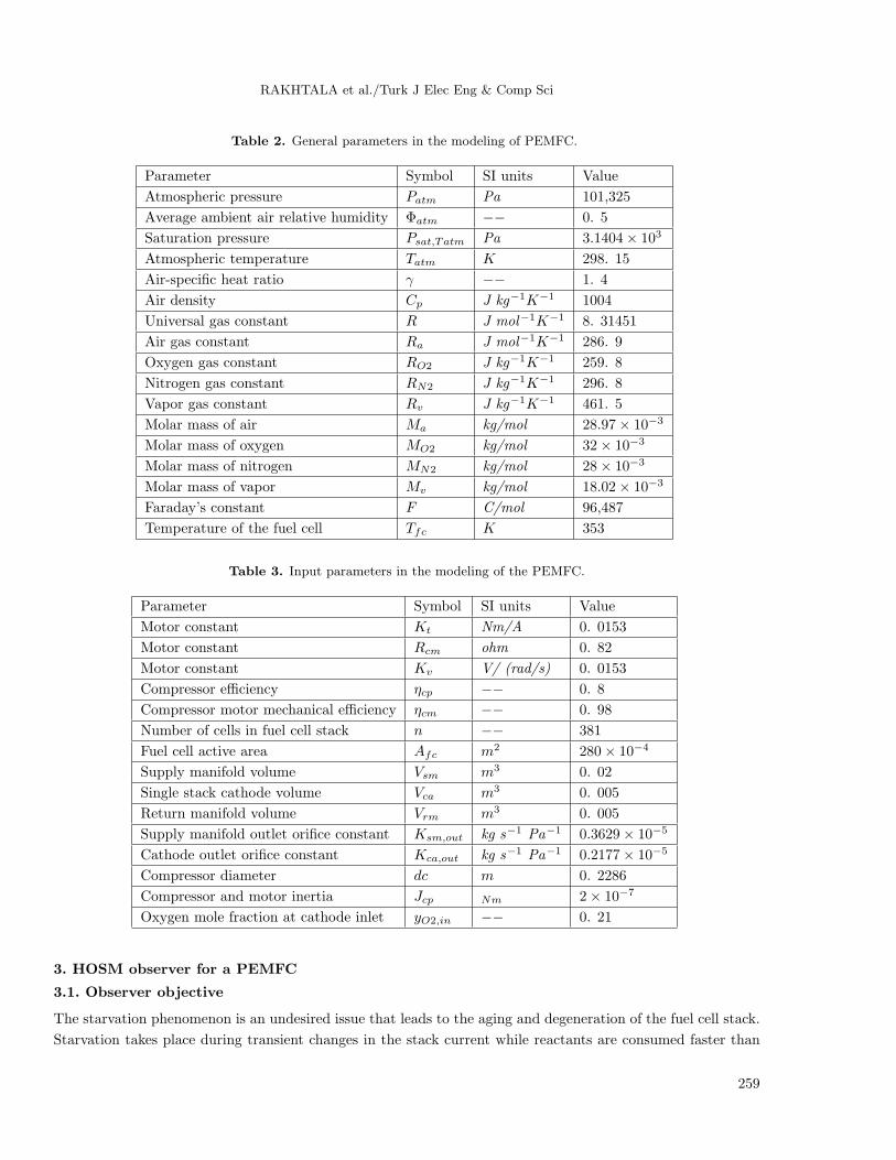
Table 2. General parameters in the modeling of PEMFC.
Parameter Symbol SI units Value
Atmospheric pressure Patm Pa 101,325
Average ambient air relative humidity Φatm −− 0. 5
Saturation pressure Psat,Tatm Pa 3.1404× 10³
Atmospheric temperature Tatm K 298. 15
Air-specific heat ratio γ −− 1. 4
Air density Cp J kg−1K−1 1004
Universal gas constant R J mol−1K−1 8. 31451
Air gas constant Ra J mol−1K−1 286. 9
Oxygen gas constant RO2 J kg−1K−1 259. 8
Nitrogen gas constant RN2 J kg−1K−1 296. 8
Vapor gas constant Rv J kg−1K−1 461. 5
Molar mass of air Ma kg/mol 28.97× 10⁻³
Molar mass of oxygen MO2 kg/mol 32× 10−3
Molar mass of nitrogen MN2 kg/mol 28× 10−3
Molar mass of vapor Mv kg/mol 18.02× 10⁻³
Faraday’s constant F C/mol 96,487
Temperature of the fuel cell Tfc K 353
Table 3. Input parameters in the modeling of the PEMFC.
Parameter Symbol SI units Value
Motor constant Kt Nm/A 0. 0153
Motor constant Rcm ohm 0. 82
Motor constant Kv V/ (rad/s) 0. 0153
Compressor efficiency ηcp −− 0. 8
Compressor motor mechanical efficiency ηcm −− 0. 98
Number of cells in fuel cell stack n −− 381
Fuel cell active area Afc m2 280× 10−4
Supply manifold volume Vsm m3 0. 02
Single stack cathode volume Vca m3 0. 005
Return manifold volume Vrm m3 0. 005
Supply manifold outlet orifice constant Ksm,out kg s−1 Pa−1 0.3629× 10⁻⁵
Cathode outlet orifice constant Kca,out kg s−1 Pa−1 0.2177× 10⁻⁵
Compressor diameter dc m 0. 2286
Compressor and motor inertia Jcp Nm 2× 10⁻⁷
Oxygen mole fraction at cathode inlet yO2,in −− 0. 21
3. HOSM observer for a PEMFC
3.1. Observer objective
The starvation phenomenon is an undesired issue that leads to the aging and degeneration of the fuel cell stack.
Starvation takes place during transient changes in the stack current while reactants are consumed faster than
259
RAKHTALA et al./Turk J Elec Eng & Comp Sci
they are supplied, causing a severe decrease in the air flow in the cathode side. The best way to avoid oxygen
starvation is fast regulation of the oxygen excess ratio through increasing the air mass flow in the cathode.
Thus, the compressor must present a fast response against rapid variations in the load current. As a control
objective, having accurate knowledge of the value of λO2 is required. It depends on the ratio of 2 mass flows
of inlet (WO2,in) and reacting (WO2,reacted) oxygen in the cathode side [10–12]. The oxygen excess ratio is
defined via the following equation:
λO2=OxygenSupplied
Oxygenreacted=
WO2,in
WO2,reacted. (10)
One way to calculate λO2 is by measuring inlet oxygen mass flow. Accordingly, the data must be acquired
through sensors. However, practical mass flow measurement causes a time delay of about 1–2 s. Furthermore,
available commercial mass flow meters are based on volumetric measurement, which is dependent on the liquid
temperature. These direct methods have some restrictions in practical applications. The other way to evaluate
λO2 is to calculate the inlet and reacting oxygen mass flow through Eqs. (11) and (12). The reacting oxygen
flow in the fuel cell stack is directly relevant to the measured stack current (Ist) [10]. Thus, it is calculated
through Eq. (11).
WO2,reacted = nMO2
4 FIst (11)
However, computation of the inlet oxygen flow is not straightforward, as it depends on states x2, x4 , andx5 .
Meanwhile, WO2,in is calculated via Eq. (12) as:
WO2,in = XO2,in1
(1 + Ωatm)Ksm,out(x2 −
x4
MO2
RO2Tst
Vca− x5
MN2
RN2Tst
Vca− Pv,ca). (12)
A substitution of Eqs. (11) and (12) into Eq. (10) immediately yields λO2 . Governing constant parameters
are defined in Tables 2–4. According to calculation of λO2 , it is seen that λO2 is related to the unmeasurable
states x4 and x5 . In this paper, due to the measurement problem of λO2 , the unavailable states are estimated
using an observer. Thus, a fast estimation of the air mass flow is required.
Table 4. Polynomial coefficients of equations.
B00 4.83× 10⁻⁵kg/sec Pa6 0. 07804 A00 0
B10 −5.42× 10⁻⁵kg/sec2 Pa5 0. 02772 A10 0.0058Nm sec
B20 8.79× 10⁻⁶kg/sec3 Pa4 0. 002122 A20 −0.0013Nm sec2
B01 3.49× 10⁻⁷kg/sec2/bar Pa3 −0.001524 A01 3.25× 10⁻⁶Nm/bar
B11 3.55× 10⁻¹³kg/sec Pa2 −0.001967 A11 −2.80× 10⁻⁶Nm sec /bar
B02 −4.11× 10⁻¹⁰kg/sec/bar Pa1 0. 001248 A02 −1.37× 10⁻⁹Nm sec /bar2
A0 4.1× 10⁻⁴Nm A1 3.92× 10⁻⁶Nm sec
3.2. Observability design requirements
The main aim of implementing an observer in our research is to estimate the oxygen and nitrogen masses at the
cathode side, which form the oxygen excess ratio. Meanwhile, the HOSM observer estimates the oxygen excess
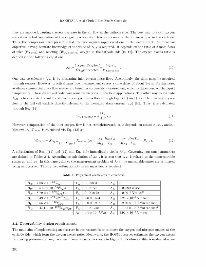
ratio using pressure and angular speed measurements, as shown in Figure 1. Its observability is evaluated when
260
RAKHTALA et al./Turk J Elec Eng & Comp Sci
the compressor angular speed, supply, and return manifold pressures are regarded as measurable outputs and
the stack current as a disturbance. Since these signals are usually available and easily measured, an output
transformation for the system in Eq. (9) is applied as follows:
d=Ist
Disturbance
Compre s s or
1 cpx ω=
Ang ula r Motor S pe e d
X2=Ps m
X3=Ms m
X4=Mo2
X5=Mn2
X6=Prm
HOS M_Obs e rve r
PEM Fue l Ce ll S ys te m
C ontroller super
T wisting=1-S MC
C ontroller
2-S MC
C ontroller
3-S MC
+
_
+
_
_
+
Output injec tor1
Output injec tor2
Output inje c tor3
U=Vc m
2oλ
Re a l e s tima te d oxyg e n e xc e s s ra tio
U=Vcm
1v
2v
3vˆ
6x
1 1y h cpω= =
2 2y h Prm= =
3 3y h Psm= =
ˆ1x
ˆ5x
Figure 1. Plant with the observer configuration.
y = h(x) =
h1(x)h2(x)h3(x)
= Cx,C = [1 0 0 0 0 0 ; 0 1 0 0 0 0 ; 0 0 0 0 0 1]T. (13)
The observability needs the rank of the following matrix with a size of 12 × 6 to be of full rank.
Osq(x) =
([dh1, · · · , dLr1−1
f h1, dh2, · · · , dLr2−1f h2, dh3, · · · , dLr3−1
f h3
]T)12×6
3∑i=1
ri = 6, 0 ≤ ri ≤ 6, i = 1, 2, 3
(14)
With reference to a generic scalar function, hi with vector argument x is defined on an open set Ω ∈ Rn and
hi : Rn → R, where dhi denotes: dhi =
dhi
dx = [ dhi
dx1, dhi
dx2, ..., dhi
dxn] . Lfhi is called the Lie derivative along f(x)
[24]. Due to the complexity of the defining system dynamics in Eqs. (1)–(6), the analytical evaluation of the
rank of matrices in Eq. (14) appears to be an exhausting job. Accordingly, the rank of all possible submatrices
is assessed. These are provided by any proper combination of rows in Eq. (14) in set M of the system state,
including operation conditions, in the presence of possible admissible perturbations.
M =x ∈ R6 : |xi − x∗
i | < Mi, i =1,2,...,6
(15)
Here, Mi(i =1,2,...,6) are known positive constants. Bound xi can be found from prior knowledge of the
system. For instance, the current can be increased up to Ist ≤ 250[A] , 5000 ≤ x1 ≤ 12000[rad/ sec], 1.4×10⁵ ≤
261
RAKHTALA et al./Turk J Elec Eng & Comp Sci
x2 ≤ 3.2 × 10⁵[Pa], 0.025 ≤ x3 ≤ 0.05[kg], 1 × 10⁻³ ≤ x4 ≤ 3.5 × 10⁻³[kg], 0.006 ≤ x5 ≤ 0.022[kg] , and
1.2× 10⁵ ≤ x6 ≤ 2.6× 10⁵[Pa] .
Therefore, an alternative analytical approach is chosen to numerically assess the operation set M to find
the minimum determinant of each square submatrix in Eq. (17). This means a solution for the following
minimization problem:
J(xopt) = minx∈M
J(x), J(x) =2
det(Osq(x)) = 0, (16)
where det stands for the determinant. To guarantee possible numerical, singularities are avoided, i.e. the
precision is chosen to be large enough. If J(xopt) is sufficiently far from 0, then the system of Eqs. (1)–(6) with
the output in Eq. (13) are observable for any x ∈ M . As a result, the following reduced square observability
matrix is found as nonsingular.
Osq(x) =[dh1, dh2, dLfh2, dh3, dLfh3, dL
2fh3
]T(6×6)
(17)
This means that states can be estimated through a properly designed observer. The matrix in Eq. (17) is full
rank in a sufficiently large set of working conditions. In the second stage, the minimum of Eq. (17) is assessed
to verify the achievement, where the minimum of the index in Eq. (16) is listed in Table 5 for different randomly
chosen starting conditions. An observer is inspired by Eq. (9) with scalar output y ∈ R, y = h(x). It is designed
using the model including an extra additive output injection term. The acting observer dynamic is written as
follows:
Table 5. Resuming for minimization.
Starting pointsMinimized value
J(x) = det2(Osq(x))
x1(0) = 5100;x2(0) = 1.48× 10⁵;x3(0) = 0.03;x4(0) = 1.2× 10⁻³;x5(0) = 0.008;x6(0) = 1.28× 10⁵ fmin = 6.8472× 1046
x1(0) = 8100;x2(0) = 1.97× 10⁵;x3(0) = 0.06;x4(0) = 1.7× 10⁻³;x5(0) = 0.01;x6(0) = 1.77× 10⁵ fmin = 1.5350× 1047
x1(0) = 11100;x2(0) = 0.49× 10⁵;x3(0) = 0.1;x4(0) = 2.7× 10⁻³;x5(0) = 0.09;x6(0) = 2.46× 10⁵ fmin = 4.9088× 1039
x1(0) = 500;x2(0) = 5.42× 10⁵;x3(0) = 0.03;x4(0) = 1.2× 10⁻³;x5(0) = 0.8;x6(0) = 4.24× 10⁵ fmin = 2.0368× 1052
˙x = f(x) + gu+G(x) v, y = h(x), (18)
where vector G(x) is the inverse of the last column of the observability matrix in Eq. (22). An output and
state estimation error is defined by:
ε = y − y = h(x)− h(x), ex = x− x, (19)
ε(j) = Ljf(x)h(x)− Lj
f(x)h(x), 1 ≤ j ≤ n− 1
ε(n) = Lnf(x)h(x)− Ln
f(x)h(x) + v(20)
It is our aim to show that the error dynamic in Eq. (20) can be stabilized and converged in a finite time
via an n−order sliding-mode algorithm. The required derivatives of the output error in the algorithm are
262
RAKHTALA et al./Turk J Elec Eng & Comp Sci
estimated through another high-order sliding-mode differentiator [25]. It is necessary to extend the approach
to multiinput-multioutput (MIMO) systems [26], where the output injection gain matrix is designed such that
the following relationship is met:
Osq(x)G(x) = N =
0 0 ... 0
...1 0 ... 0
r1×p
0 0 ... 0...0 1 ... 0
r2×p
· · ·
0 0 ... 0...0 0 ... 1
rp×p
T
︸ ︷︷ ︸N Matrix
, (21)
G(x) = (Osq(x))−1N, (22)
where p is the dimension of the output vector and ri(i = 1, 2, ..., p). This shows that the observation indices of
the nonsingular matrix are of full rank.
Assumption 1 Matrix Osq(x) in Eq. (21) is nonsingular for every possible value of x .
The proposed analytical approach in the previous subsection shows the observability indices as r1 =
1, r2 = 2, and r3 = 3 for the PEMFC model in Eqs. (1)–(6) and (13). Therefore, the condition in Eq. (21) of
the output injection gain matrix G(x) has the following form:
Osq(x)G(x) = N = [1 0 0 ; 0 0 0 ; 0 1 0 ; 0 0 0 ; 0 0 0 ; 0 0 1]T. (23)
Lemma 1 Consider system Eq. (9) and assume Osq(x) to be nonsingular for every possible value of M . Next,
the following implication holds:
ε = 0 ⇔ ex = 0. (24)
The state of the system in Eq. (9) can be reconstructed in finite time by applying the observers in Eqs. (18)
and (22), provided that the correction term vi is designed in such a way that error vector ε will be steered to 0
in finite time. 2
Indeed, Lemma 1 proves the finite time convergence of the proposed observer. This means that the
estimated states approach the real states in a limited time when the output injected terms vi force the output
error vector to tend to 0 in finite time. The proof of Lemma 1 is stated in Appendix 1.
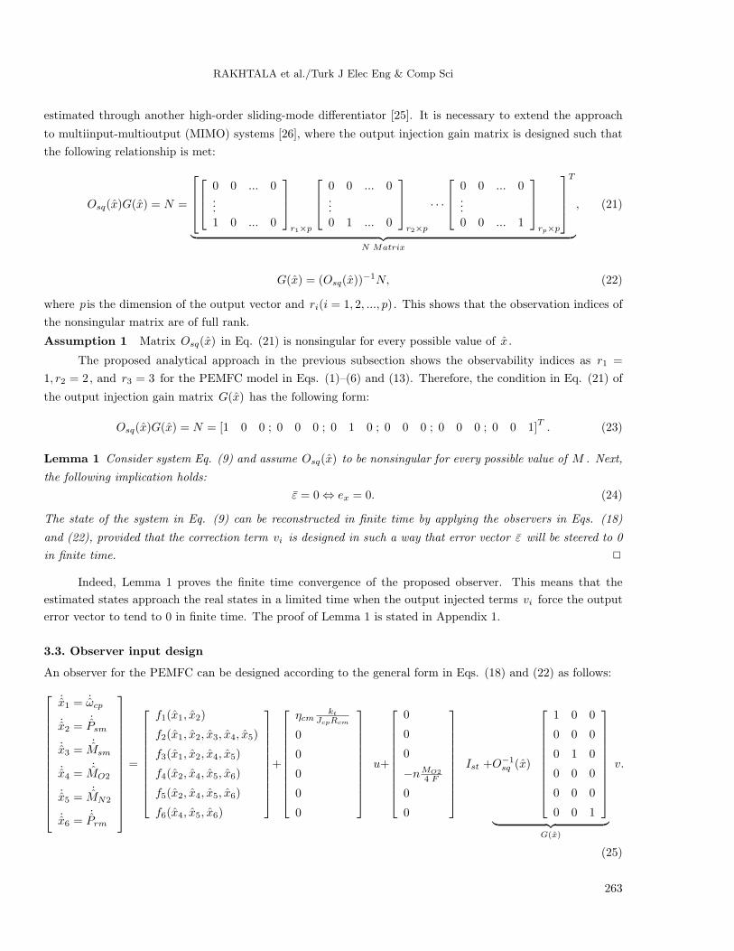
3.3. Observer input design
An observer for the PEMFC can be designed according to the general form in Eqs. (18) and (22) as follows:
˙x1 = ˙ωcp
˙x2 =˙Psm
˙x3 =˙Msm
˙x4 =˙MO2
˙x5 =˙MN2
˙x6 =˙Prm
=
f1(x1, x2)
f2(x1, x2, x3, x4, x5)
f3(x1, x2, x4, x5)
f4(x2, x4, x5, x6)
f5(x2, x4, x5, x6)
f6(x4, x5, x6)
+
ηcmkt
JcpRcm
0
0
0
0
0
u+
0
0
0
−nMO2
4 F
0
0
Ist +O−1
sq (x)
1 0 0
0 0 0
0 1 0
0 0 0
0 0 0
0 0 1
︸ ︷︷ ︸
G(x)
v.
(25)
263
RAKHTALA et al./Turk J Elec Eng & Comp Sci
The estimation error dynamics include the relative degree of the vector by r=1, 2, 3 . The output vector
y = [y1 = ωcp, y2 = Prm, y3 = Psm] forms output derivatives by:
e1 = y1 − y1 = ωcp − ωcp, e2 = y2 − y2 = Prm − Prm, e3 = y3 − y3 = Psm − Psm. (26)
The vector of relative degree of 1, 2, 3 is respectively relevant to the output vector y1, y2, y3 . It drives theobserver control input vi to be selected according to the relative degree. Each output injection term vi can
be designed by a high-order sliding-mode algorithm, such that the estimation error approaches 0 in a finite
time. Therefore, output injection laws in the following are chosen according to each specific value of ri (i.e. the
relative degree):
• r1 = 1 allows for using a super twisting algorithm [27] by
v1 = −α1 |e1|12 sign(e1)− λ1
∫sign(e1)dt. (27)
• r2= 2 permits the use of a suboptimal algorithm [27] as
v2 = −α2U2sign(e2 − β2.e2,M ), β2 ∈ [0, 1) . (28)
• r3= 3 is suggested [28] to use a quasicontinuous algorithm. Since the output error e3 = y3−y3 = Psm−Psm
contains a relative degree of 3, values are selected according to the third-order quasicontinuous sliding-
mode algorithm as:
v3 = −α3e3 + 2(|e3|+ |e3|
23 )
12 (e3 + |e3|
23 sign(e3))
|e3|+ 2(|e3|+ |e3|23 )
12
. (29)
To implement the algorithm in Eq. (29), the values of e3, e3 , and e3 must be configured. Since these
terms are not actually available, a robust differentiation of e3 is used to reconstruct the nonmeasurable variables.
The following homogeneous differentiator of e3 is proposed:
z3,0 = v3,0 where v3,0 = −λ3,0 |z3,0 − e3|23 sign(z3,0 − e3) + z3,1
z3,1 = v3,1 and v3,1 = −λ3,1 |z3,1 − v3,0|12 sign(z3,1 − v3,0) + z3,2
(30)
Parameters of the algorithm in Eq. (29) and differentiator in Eq. (30) are tuned according to the bounds
of the observer dynamics. Proper positive constant coefficients λ3,i are chosen large enough in the given
order [25] under the assumption that a constant L exists such that∣∣e(n)∣∣ < L . After a finite-time transient
process, the following equalities are satisfied, of course in the absence of measurement noise:∣∣∣Z3 − e
(i)3
∣∣∣ = 0
and i = 0, 1, ..., n . It was demonstrated by Levant in [25] that nonidealities, such as measurement noise and
finite frequency commutation, cause a bounded error in the estimated derivatives. As a result, a bounded loss
of accuracy occurs, which causes the algorithm to use ‘noisy’ derivative estimates [25,28].
264
RAKHTALA et al./Turk J Elec Eng & Comp Sci
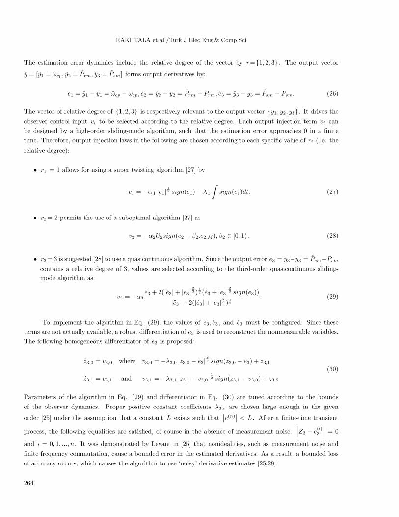
4. Structure of the overall control scheme
Starvation is one of the main causes of aging of the fuel cell. Oxygen starvation causes performance degradation
in the fuel cell and a cell voltage drop occurs. To avoid the oxygen starvation phenomenon, the oxygen excess
ratio should be adjusted quickly. Thus, regulating the compressor voltage vcm causes a rapid increase in the
mass flow into the cathode and the prevention of oxygen starvation. This regulation prolongs the fuel cell life
and optimizes the performance. When a step change in current Ist occurs, compressor voltage vcm has to
be properly adjusted to regulate the oxygen excess ratio. The proposed overall control scheme consists of the
following 2 nested loops using SOSM-based control:
1. An inner loop generates the reference compressor voltage by controlling the angular speed.
2. An outer loop provides a reference angular motor speed by controlling the oxygen excess ratio.
An effective solution to stabilize the control loop is a cascade structure via using a super twisting
controller. In this configuration, 2 nested loops are provided, as shown in Figure 2. The inner loop forms
a proper control signal to accordingly change the angular speed of the motor. The outer loop is designed to
control the excess ratio when the constructed λO2 is compared with the reference λ∗O2 to form the error signal.
The error is then processed by a super twisting controller to generate an angular speed reference applied to the
inner loop.
W=Ist
Disturbance
C ompres s or
1 cpx ω=A ngular Motor
S peed
FC Model
U=V c mHOS M_Obs erver
2
oλ
R eal es timated
oxygen exc es s
ratio
2
ˆOλ
S uper
twis ting+_
S uper
twis ting
+
_
cpω*
22.05
Oλ*
=
1
P2
Pr6
x cp
y x sm
x m
ω=
= =
=
ˆ6x
ˆ2x
ˆ1x
Figure 2. Block diagram of the proposed cascade structure using a super twisting controller.
4.1. Cascade structure
The super twisting controller consists of a control output u with 2 terms, without the need for information on
S . The first term is a discontinuous time-derivative term, while the second is a continuous function of a sliding
variable. Thus, the ucontrol law is defined by the following expression:
u = −λ |S|12sign(S)−W
t∫0
sign(S(τ))dτ, (31)
where W and λ are design parameters. The first-time derivative of the sliding variable is expressed by
S = ϕ(t, x) + γ(t, x)u . Terms γ(t, x) and ϕ(t, x) are functions in time and the states. For PEMFC system
applications, they are bounded smooth functions as 0 < Γm ≤ γ(t, x) ≤ ΓM and |ϕ(t, x)| ≤ Φ, where Φ, ΓM ,
and Γmare appropriate bounds. Sufficient conditions for finite time convergence of the sliding manifold S can
be seen in [29]:
W >Φ
Γm, λ2 ≥ 4Φ
Γ2m
ΓM (W +Φ)
Γm(W − Φ). (32)
265
RAKHTALA et al./Turk J Elec Eng & Comp Sci
The required controller parameters are properly designed to meet the conditions in Eq. (32). Therefore, conver-
gence of the super twisting controller in finite time is guaranteed. This controller provides proper performance
in systems with relative degrees of 1 and shows good robustness against disturbances and uncertainties [27].
Furthermore, this is found effective for chattering attenuation purposes.
4.1.1. Inner control loop
The aim of this loop is to provide the oxygen ratio through the compressor. The inner loop provides the measured
angular speed (ωcp) in a quicker time through a separate controller using the reference angular speed(ω∗cp).
This loop produces an actual control input vcm to ensure quick convergence of the measured angular speed to
the reference angular speed. This control objective will be achieved under the variable structure system (VSS)
theory framework, i.e. sliding-mode control. To implement this controller, first a sliding surface must be defined
as a discrepancy between the real motor speed and that of the command. This can be found by:
S2 = ωcp − ω∗cp. (33)
Once the differentiation of the sliding variable S2 = ωcp−ω∗cp of the inner loop is complete, the control input vcm
will appear in the first derivative, as seen in Eq. (A7) of Appendix 2. This equation verifies that the relative
degree between the angular speed and the compressor voltage is 1. A detailed description of the first-order
derivative S2 along with coefficients γ2(t, x) and φ2(t, x) is given in Appendix 2.
0 < Γ2,m ≤ γ2(t, x) ≤ Γ2,M , |ϕ2(t, x)| ≤ Φ2 (34)
To form the control in Eq. (34), the parameters of the controller have to be determined using sufficient conditions
in Eq. (32). Therefore, it is necessary to find the bound of the first derivative of the sliding surface, such that
the following bounded conditions on the sliding dynamics are satisfied. The closed-loop error dynamics are then
bounded by:
S2 ∈ [−Φ2,Φ2] + [−Γ2,m,Γ2,M ] vcm, (35)
considering the positive constants Γ2,m,Γ2,M , and Φ2 . Substitution of the states in S2 (Appendix 2) evaluates
the bounds of γ2 and Φ2 in 0 < Γ2,m ≤ γ2(t, x) ≤ Γ2,M and |ϕ2(t, x)| ≤ Φ2 . On the other hand, a bound for the
sliding surface is arbitrarily chosen, which is seen here as S2,0 = 1× 10⁻³ . This yields 5717.69 ≤ γ2 ≤ 6675.88
and Φ2 = 0.6455. To achieve finite time convergence of the angular speed, the following theorem must be
satisfied.
Theorem 1 The error of the angular speed tracking in the inner loop converges to S2 = 0 in finite time. An
upper bound of the convergence time is assessed by the following:
T0,inner =2 V
12 (ζinner(0))
α=
2√ζTinner(0) Q ζinner(0)
α, α =
λmin Q λ12
min P2λmax P
, (36)
where ζinner(0) is an initial condition of ζinner . 2
266
RAKHTALA et al./Turk J Elec Eng & Comp Sci
Proof of Theorem 1:
Consider the following super twisting controller:
Z1 = −K1 |Z1|12 sign(Z1) + Z2, Z2 = −K2sign(Z1), (37)
where Z1 ∈ R and Z2 ∈ R concerning the equilibrium point at (Z1, Z2) = (0, 0). A detailed stability proof of
the super twisting controller can be found in [30–32]. Now consider the following family of quadratic Lyapunov
functions [30]:
V = ζTPζ, (38)
such that ζ = [|Z1|12 sign(Z1), Z2]
T , where P is a positive definite matrix [33]. Function V (t) is continuous and
differentiable, except when Z1 = 0. In fact, for Z1 = 0, its derivative, V (ζ, t), exists and is negative-definite.
It can be seen that although the state trajectory of Eq. (38) attaches to the surfaceS2 , it cannot stay on it.
Before reaching the equilibrium point (Z1, Z2) = (0, 0), Eq. (37) coincides with the line Z1 = 0 for Z2 = 0.
This means that the derivative of the Lyapunov function exists everywhere until the state trajectory reaches
the equilibrium point. In accordance with [30,31,33], V (t) is a strong Lyapunov function of the form of Eq.
(38) for Eq. (37). Although this Lyapunov function is positive-definite, it is radially unbounded.
λmin(P ) ∥ζ∥22 ≤ V ≤ λmax(P ) ∥ζ∥22 , (39)
when ∥ζ∥22 = |Z1|+Z22 stands for an Euclidian norm of ζ . The construction of proper positive definite matrices
P = PT solves the algebraic Lyapunov equation (ALE) of [30,31,33]:
ATP + PA = −Q, (40)
where A =
[−K1 1−K2 0
], K1 > 0 and K2 > 0, are positive gains. This means that matrix A is Hurwitz,
where Q = QT > 0 is an arbitrary chosen symmetric and positive definite matrix. Using the vector ζ =
[|Z1|12 sign(Z1), Z2]
T , since ζ =
[−K1 1−K2 0
]ζ
/(2 |Z1|
12 ) = Aζ
/(2 |Z1|
12 ), the derivative of the Lyapunov
function is obtained as:
V (ζ) = ζTPζ + ζTP ζ =1
2 |Z1|12
ζT (ATP + PA)ζ = − 1
2 |Z1|12
ζTQζ. (41)
According to Eq. (39) and the Euclidian norm of ζ , it is seen that ∥ζ∥2 ≤ V12 (ζ)
/(λ
12
min P). Therefore,
V (ζ, t) is deduced by:
V (ζ) = − 1
2 |Z1|12
ζTQζ ≤ −λmin Q2 |Z1|
12
∥ζ∥22 ≤ −λmin Qλ12
min P
2λ12max P
V12 (ζ), (42)
where α = λmin Qλ12
min P/(2λ
12max P) and V ≤ −αV
12 (ζ). Therefore, the finite time convergence of
vector (Z1, Z2) to 0 is guaranteed and bounded by T0 = 2V12 (ζ(0))
/α , assuming that ζ(0) is the initial value
267
RAKHTALA et al./Turk J Elec Eng & Comp Sci
ofζ . It was suggested in [32] that the identity matrix selection as Q = I is a proper choice to achieve a minimum
time for a class of Lyapunov functions. Choosing K1 = 0.45 and K2 = 0.8 results in P =[2 12 ;−
122.781
]Tby
P = PT > 0 as a solution of the ALE. The initial conditions of Z1(0) = 0.69 and Z2(0) = 0.14, an estimation
of the upper bound of the convergence time T0,inner = 2V12 (ζinner(0))
/α , is found as T0,inner = 3.46.
4.1.2. Outer control loop
The main task of the outer loop is to derive the oxygen excess ratio λO2 to its desired oxygen excess ratio
reference value λ∗O2 through the generation and adjustment of the compressor angular speed. Indeed, a super
twisting controller must force the sliding variables S1 = λO2 − λ∗O2 to 0 in finite time. Primarily, a relative
degree is equal to 1 when the first derivative of variable S1 is taken (Eq. (A8) of Appendix 2). By replacing x2
from Eq. (2) into Eq. (A8), a direct relationship between λO2 and ωcp will be achieved. The result shows the
relative degree of 1 between the oxygen excess ratio and the angular motor speed. Similarly, there is a relative
degree of 2 between the oxygen excess ratio and the compressor voltage. The closed-loop error dynamics in the
outer loop are then bounded by:
S1 ∈ [−Φ1,Φ1] + [−Γ1,m,Γ1,M ]ωcp. (43)
The system bound, similar to S2,0 , is arbitrarily chosen as S1,0 = 1 × 10⁻³ . This again obtains the following
bound:
0 < Γ1,m ≤ γ1(t, x) ≤ Γ1, M , |ϕ1(t, x)| ≤ Φ1
3.492× 10⁻⁷ ≤ γ1 ≤ 6.984× 10− 5 , Φ1 = 2.345× 10− 7. (44)
Detailed descriptions of the first-order derivatives S1 and S2 , along with the coefficients γ1(t, x), ϕ1(t, x), and
γ2(t, x), ϕ2(t, x), are given in Appendix 2. In order to obtain a finite-time convergence of reaching the estimated
oxygen excess ratio to the sliding surface, the following theorem must be valid.
Theorem 2 Similar to the method in Theorem 1, the oxygen excess ratio in the outer loop converges to
equilibrium λ∗O2 in a finite time of T0,outer , which is expressed in the following:
T0,outer =2√
ζTouter(0) Q ζouter(0)
α, α =
λmin Q λ12
min P2λmax P
. (45)
Proof The determination of the convergence time of the outer loop can be proven in the same way as in
Theorem 1.
Coefficients of super twisting in the inner and outer loops of the cascade structure are found by a trade-off
between the dynamic performance and chattering as λ1 = 2,W1 = 2, and λ2 = 4,W2 = 4.
Proposition 1 The sliding mode controller in Eq. (31) guarantees that the system in Eq. (9) tracks and
converges to the reference command in finite time if the observer in Eq. (25) constructs unavailable states in
finite time. On the other hand, when the observer dynamics are fast enough to provide an accurate evaluation
of the modes, the controller stabilizes the whole closed-loop system.
268
RAKHTALA et al./Turk J Elec Eng & Comp Sci
Satisfaction 1 According to Lemma 1 and the finite time convergence of observer, it is not necessary to prove
the separation principle [25,34,35]. Considering the separation principle using HOSM observers in a VSS, a
general statement is that if the observation is achieved in a finite time and the system is bounded-input bounded-
output stable, it is possible to design an observer and controller separately. This means that after a finite time,
the estimation error vanishes and, therefore, the state feedback can be implemented using the state estimates
[34,35]. Next, it is sufficient to prove a finite time convergence of the observer (Lemma 1) and the stability of
the system in a closed loop (Section 4.1) with super twisting control separately.
4.2. Suboptimal controller
To investigate the validity and performance of the proposed cascade structure, a suboptimal controller is used
as an alternative technique. The control objective is S(x, t) = λO2 − λ∗O2 , which again needs to become 0.
As previously stated, the control signal u = vcm appears in the second-order derivative of the sliding variable
S(x, t) = λO2 − λ∗O2 ; therefore, the relative degree is again found as 2. A block diagram of the system under
suboptimal control is shown in Figure 3. Moreover, during a real-time application, the suboptimal controller
only requires knowledge of the sign of the sliding variable. The main advantage of this approach relies on its
robustness against some parametric uncertainties and external disturbances. This controller is used for plants
with a relative degree of 2, as in the following [27]:
W=Ist
Disturbance
Compre s s or
FC Mode l
U=Vcm
2
oλ
Re a l e s tima te d oxyg e n e xc e s s
ra tio
Suboptimal+
_
22.05
Oλ *
=
HOS M_Obs e rve r
ˆ1x
ˆ2x
ˆ6x
1
P2
Pr6
x cp
y x sm
x m
ω=
= =
=
1 cpx ω=
2
ˆOλ
Figure 3. Block diagram of the controlled system with a suboptimal controller.
u (t) = −α(t)U sign(S − βSM )
β ∈ [0, 1) , α (t) =
1 if (S − βSM )SM ≥ 0
α∗ if (S − βSM )SM < 0
, (46)
where α∗, β , and U are controller parameters. These must be tuned according to the following inequalities:
U >Φ
Γm, α∗ ∈ [1,+∞) ∩
[Φ+ (1− β)ΓMU
βΓmU,+∞
). (47)
Finally, the parameters of the suboptimal controller in Eq. (47) are selected as β = 0.9, U = 1, and α∗ = 1.
269
RAKHTALA et al./Turk J Elec Eng & Comp Sci
5. Simulation results
In order to verify the performance of the proposed configuration, including 2 individual controllers (used in the
cascade and also the suboptimal) in combination with the proposed finite-time observer, several simulations are
carried out. Since the temperature and humidity are assumed to be constant, a separate controller is designed to
keep them unchanged to validate those assumptions. Meanwhile, the bounds of the estimation error dynamics
are overestimated due to consideration of the worst-case design during the state variations within set M in Eq.
(16). Meanwhile, the parameters of the output injection law in Eqs. (27)–(30) are manually tuned. All of the
simulations are performed in Table 6 with the set configuration and parameters of the output injection law.
The load current is stepped up from 100 A to 150 A at t = 20 s, after 35 s. It is again stepped down to 120 A,
and, finally, at time t = 80 s, the current is stepped up from 120 A to 190 A (Figure 4).
Table 6. Output injectors and parameter settings according to the relative degrees.
Relative degree Type of controller Parameter tunings
r1 = 1 Super twisting algorithm λ1 = 3, α1 = 3
r2 = 2 Suboptimal algorithm β2 = 0.5, U2 = 0.1, α2 = 1
r3 = 3 Quasi-continuous algorithmn = 2, λ3,0 = 15.9, λ3,1 = 33.5,
λ3,2 = 550, α3 = 1500
0 20 40 60 80 100 12080
100
120
140
160
180
200
Time (s)
Ist
(A)
Stack current
Figure 4. Load current variation profile.
5.1. Observer analysis for estimation of the oxygen excess ratio
In the observer analysis, the voltage driving the DC motor of the compressor is maintained constant at 150 V.
The goal of the observer design is to estimate an unmeasurable state of the PEMFC, i.e. the oxygen excess ratio,
which is expressed from Eqs. (10) through (12). Actual and estimated values of the oxygen excess ratio are
illustrated in Figure 5. It is seen that the important variable to improve the efficiency of the PEMFC is precisely
estimated. To verify the tracking ability of the observer, the oxygen excess ratio is estimated using the HOSM
observer, which is depicted in Figure 5. Since the error band is narrow, the outcome of the estimation is found
satisfactory. Figure 5 also shows that the estimator follows the oxygen excess ratio with an acceptable lag. The
observer converges to the correct amount of the oxygen excess ratio in a finite time, i.e. after approximately 3
s. It is seen that the proposed observer is capable to estimate some important states of the PEMFC and the
oxygen excess ratio in finite time. Furthermore, a sliding-mode technique is developed in the observer design.
This also produces an output injection with a high switching frequency and zero mean value.
270
RAKHTALA et al./Turk J Elec Eng & Comp Sci
0 20 40 60 80 100 1201
1.5
2
2.5
3
3.5
4
Time (s)
Oxy
gen
exce
ssr a
tio
λO2
Real
λO2
Estimated0 1 2 3 4 5
2
2.5
3
3.5
Ox
ygen
ex
cess
rat
io λO2λO2 Estimated
Figure 5. Estimation of the oxygen excess ratio signal.
5.2. Output feedback control system
An optimum value of λ∗O2 = 2.05 [4,5] is assumed as a reference. It can be assured that the system works at its
maximum net power for each load variation. To verify the performance of the proposed control structure, some
simulations are carried out. The following results are achieved from different implementations of the closed-loop
system.
In TEST 1, since the relative degree equals 2, a suboptimal controller is implemented as in Figure 6a.
0 20 40 60 80 100 1201
1.5
2
2.5
3
Time (s)
Oxy
gen
exce
ssr a
tio
λO2 controlled with suboptimal
λO2 Reference
a
0 20 40 60 80 100 1200
0.5
1
1.5
2
2.5
3
Time (s)
Oxy
gen
exce
ssra
tio
λO2
controlled with cascade
λO2
Referenceb
0 20 40 60 80 100 1200
0.5
1
1.5
2
2.5
3
Time (s)
Oxy
gen
exce
ssra
t io
λO2 with observer in closed loop
λO2
without observerc
79 80 81 82 83 84 851
1.5
2
2.5
Time (s)
Oxy
gen
exce
ssra
tio
Figure 6. a) Oxygen excess ratio control via the suboptimal controller, b) cascade structure, and c) oxygen excess ratio
control with an observer and without an observer.
271
RAKHTALA et al./Turk J Elec Eng & Comp Sci
In TEST 2, a cascade structure with a super twisting controller is implemented. The dynamic behavior
of the oxygen excess ratio under different load conditions is also depicted in Figure 6b. It can be observed that
this variable follows the reference well enough with satisfactory tracking performance.
According to the graphs, it is found that the suboptimal controller produces a faster time response with
respect to the cascade structure. However, the error band in the cascade structure using the super twisting
controller is found as smaller and narrower with respect to the suboptimal controller. From the simulation
results, it can be stated that the suboptimal controller presents good dynamic behavior. This controller reduces
the rise time and settling time of tuning the oxygen excess ratio during the transient step changes of the current
with respect to the cascade structure (Table 7).
Table 7. Time domain performance specifications.
Controller type Rise time (ms) Settling time (ms) (3%) Output deviations
Cascade 3950 5130 ±2.5× 10⁻⁴
Suboptimal 61 1220 ±3× 10⁻³
In the meantime, the performance of the proposed observer can be compared with that of the actual
states in [11]. The result in Figure 6c shows that without using the observer, the system tracks the reference
value of λO2 in about 3 s, whereas in the closed-loop implementation, using the observer significantly reduces
the tracking time to 0.4 s.
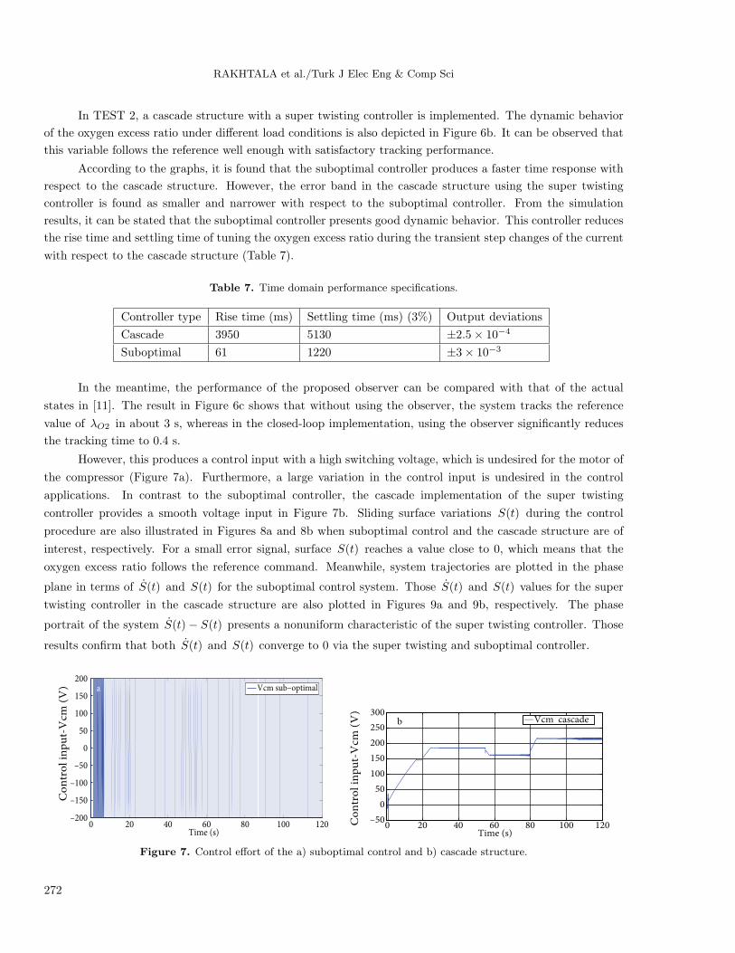
However, this produces a control input with a high switching voltage, which is undesired for the motor of
the compressor (Figure 7a). Furthermore, a large variation in the control input is undesired in the control
applications. In contrast to the suboptimal controller, the cascade implementation of the super twisting
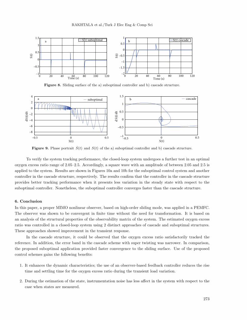
controller provides a smooth voltage input in Figure 7b. Sliding surface variations S(t) during the control
procedure are also illustrated in Figures 8a and 8b when suboptimal control and the cascade structure are of
interest, respectively. For a small error signal, surface S(t) reaches a value close to 0, which means that the
oxygen excess ratio follows the reference command. Meanwhile, system trajectories are plotted in the phase
plane in terms of S(t) and S(t) for the suboptimal control system. Those S(t) and S(t) values for the super
twisting controller in the cascade structure are also plotted in Figures 9a and 9b, respectively. The phase
portrait of the system S(t)− S(t) presents a nonuniform characteristic of the super twisting controller. Those
results confirm that both S(t) and S(t) converge to 0 via the super twisting and suboptimal controller.
0 20 40 60 80 100 120–200
–150
–100
–50
0
50
100
150
200
Time (s)
Vcm sub–optimala
0 20 40 60 80 100 120–50
0
50
100
150
200
250
300
Time (s)
Vcm cascade b
Co
ntr
ol
inp
ut-
Vcm
(V
)
Co
ntr
ol
inp
ut-
Vcm
(V
)
Figure 7. Control effort of the a) suboptimal control and b) cascade structure.
272
RAKHTALA et al./Turk J Elec Eng & Comp Sci
0 20 40 60 80 100 120–1
–0.5
0
0.5
1
1.5
Time (s)
S(t
)
S(t) suboptimala
0 20 40 60 80 100 120–2
–1.5
–1
–0.5
0
0.5
1
Time (s)
S(t
)
S(t) cascadeb
Figure 8. Sliding surface of the a) suboptimal controller and b) cascade structure.
–0.5 0 0.5
–8
–6
–4
–2
0
2
4
S(t)
dS
(t)/
dt
suboptimala
–0.5 0 0.5–1
–0.5
0
0.5
1
1.5
S(t)
dS
(t )/d
t
cascadeb
Figure 9. Phase portrait S(t) and S(t) of the a) suboptimal controller and b) cascade structure.
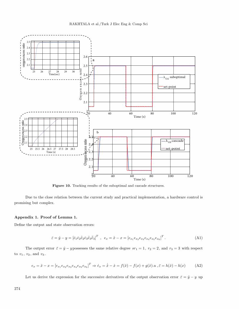
To verify the system tracking performance, the closed-loop system undergoes a further test in an optimal
oxygen excess ratio range of 2.05–2.5. Accordingly, a square wave with an amplitude of between 2.05 and 2.5 is
applied to the system. Results are shown in Figures 10a and 10b for the suboptimal control system and another
controller in the cascade structure, respectively. The results confirm that the controller in the cascade structure
provides better tracking performance when it presents less variation in the steady state with respect to the
suboptimal controller. Nonetheless, the suboptimal controller converges faster than the cascade structure.
6. Conclusion
In this paper, a proper MIMO nonlinear observer, based on high-order sliding mode, was applied in a PEMFC.
The observer was shown to be convergent in finite time without the need for transformation. It is based on
an analysis of the structural properties of the observability matrix of the system. The estimated oxygen excess
ratio was controlled in a closed-loop system using 2 distinct approaches of cascade and suboptimal structures.
These approaches showed improvement in the transient response.
In the cascade structure, it could be observed that the oxygen excess ratio satisfactorily tracked the
reference. In addition, the error band in the cascade scheme with super twisting was narrower. In comparison,
the proposed suboptimal application provided faster convergence to the sliding surface. Use of the proposed
control schemes gains the following benefits:
1. It enhances the dynamic characteristics; the use of an observer-based feedback controller reduces the rise
time and settling time for the oxygen excess ratio during the transient load variation.
2. During the estimation of the state, instrumentation noise has less affect in the system with respect to the
case when states are measured.
273
RAKHTALA et al./Turk J Elec Eng & Comp Sci
20 40 60 80 100 1202
2.1
2.2
2.3
2.4
2.5
2.6
Time (s)
Time (s)
Ox
yg
en
ex
ce
ss
rati
oλ
O2 suboptimal
set-point
a
20 40 60 80 100 1202
2.1
2.2
2.3
2.4
2.5
Ox y
g en
exce
ssra
ti o λO2
cascade
set-point
b
25 26 27 28 29 30
2.1
2.2
2.3
2.4
2.5
Time(sec)
25 25.5 26 26.5 27 27.5 28 28.5
2.1
2.2
2.3
2.4
2.5
Time (s)
Oxy
gen
exce
s sr a
ti oox
yge n
exce
s sr a
ti o
Figure 10. Tracking results of the suboptimal and cascade structures.
Due to the close relation between the current study and practical implementation, a hardware control is
promising but complex.
Appendix 1. Proof of Lemma 1.
Define the output and state observation errors:
ε = y − y = [e1e2 ˙e2e3 ˙e3 ¨e3]T
, ex = x− x = [ex1ex2ex3ex4ex5ex6 ]T. (A1)
The output error ε = y − ypossesses the same relative degree sr1 = 1, r2 = 2, and r3 = 3 with respect
to v1 , v2 , and v3 .
ex = x− x = [ex1ex2ex3ex4ex5ex6 ]T ⇒ ex = ˙x− x = f(x)− f(x) + g(x).u , ε = h(x)− h(x) (A2)
Let us derive the expression for the successive derivatives of the output observation error ε = y − y up
274
RAKHTALA et al./Turk J Elec Eng & Comp Sci
to the order n , which yields:
e1
e2
˙e2
e3
˙e3
¨e3
=
h1(x)− h1(x)
h2(x)− h2(x)
L1f(x)h2(x)− L1
f(x)h2(x)
h3(x)− h3(x)
L1f(x)h3(x)− L1
f(x)h3(x)
L2f(x)h3(x)− L2
f(x)h3(x)
,
˙e1
¨e2
e3
=
L1f(x)h1(x)− L1
f(x)h1(x)
L2f(x)h2(x)− L2
f(x)h2(x)
L3f(x)h3(x)− L3
f(x)h3(x)
+
v1
v2
v3
. (A3)
If ex = x − x ⇒ x = x − ex , the above equations allow for constructing diffeomorphic mappings [24] in
the following:
ε = Φ(ex, x) =
e1
e2
˙e2
e3
˙e3
¨e3
=
Φ11(ex, x)
Φ21(ex, x)
Φ22(ex, x)
Φ31(ex, x)
Φ32(ex, x)
Φ33(ex, x)
=
h1(x)− h1(x− ex)
h2(x)− h2(x− ex)
L1f(x)h2(x)− L1
f(x−ex)h2(x− ex)
h3(x)− h3(x− ex)
L1f(x)h3(x)− L1
f(x)h3(x− ex)
L2f(x)h3(x)− L2
f(x)h3(x− ex)
. (A4)
If ex = 0, then all components of vector ε are identically 0 irrespectively of x , i.e. Φ(0 , x) = 0. For the
details of the proof, see [36]. Lemma 1 is guaranteed provided that the mapping Φ(ex , x) is locally bijective
in the neighborhood of ex = 0. The bijectivity of the mapping will be defined as detJ(0, x) = 0, ∀x using the
Jacobean matrix J(ex, x) =∂(Φ(ex , x))
∂ex[36]. The Jacobean matrix is expressed as:
J(ex, x) =∂(Φ(ex, x))
∂ex=
∂(Φ11(ex, x))/∂ex
∂(Φ21(ex, x))/∂ex
∂(Φ22(ex, x))/∂ex
∂(Φ31(ex, x))/∂ex
∂(Φ32(ex, x))/∂ex
∂(Φ33(ex, x))/∂ex
=
∂(−h1(x− ex))/∂ex
∂(−h2(x− ex))/∂ex
∂(−L1f(x−ex)
h2(x− ex))/∂ex
∂(−h3(x− ex))/∂ex
∂(−L1f(x)h3(x− ex))
/∂ex
∂(−L2f(x)h3(x− ex))
/∂ex
, (A5)
∂(Φ11(ex, x))
∂ex= −∂(h1(x))
∂x
∂(x− ex)
∂ex. (A6)
The replacement of x = x − ex in the above equation, and equating ex = 0 and ∂(x− ex)/∂ex = −1,
yields J(ex, x)|ex=0 = Osq(x). This confirms the nonsingularity of J(ex, x)|ex=0 = Osq(x), as stated in
Assumption 1. Therefore, the observer in Eq. (18) with the observability matrix in Eq. (21) reconstructs the
state of the system in Eq. (9) in finite time. It is seen that the observer input vi is selected in such a way that
the vector ε is steered to 0 in finite time.
275
RAKHTALA et al./Turk J Elec Eng & Comp Sci
Appendix 2. Sliding variable and its time derivatives
• Inner loop:
S2 = ωcp − ω∗cp ⇒ S2 = ϕ2(t, x) + γ2(t, x) vcm
γ2(t, x) =π
30 Jcp(ηcm
kt
JcpRcm)
ϕ2(t, x) =π
30 Jcp(−ηcm
kt
JcpRcmkvx1
−(A0 +A1x1 +A00 +A10x1 +A20(x1)2 +A01x2 +A11x2x1 +A02(x2)
2))
(A7)
• Outer loop:
S1 = λO2 − λ∗O2 = ϕ1(t, x) + γ1(t, x)ωcp
S1 = λO2 − λ∗O2 =
XO2,in(1+Ωatm)−1 Ksm,out(x2− x4MO2
RO2.TstVca
− x5MN2
RN2TstVca
−Pv,ca)
WO2,reacted
γ1 =XO2,in
WO2,reacted
Ksm,outB01(Tatm−Tatmηcp
)
1+Ωatm
(A8)
The detailed calculation of ϕ1 is similar to that of ϕ2 . Therefore, the detailed calculation of ϕ1 is ignored
to avoid complexity.
ϕ1 =
[∂S1
∂x1
∂S1
∂x2
∂S1
∂x3
∂S1
∂x4
∂S1
∂x5
∂S1
∂x6
]× [f(x, t) + g(x, t)ωcp] (A9)
References
[1] Larminie J, Dicks A. Fuel cell systems explained. 2nd ed. New York, NY, USA: Wiley, 2003.
[2] Wang C, Nehrir MH, Shaw SR. Dynamic models and model validation for PEM fuel cells using electrical circuits.
IEEE T Energy Convers 2005; 20: 442–451.
[3] Rakhtala SM, Ghaderi R, Ranjbar A, Fadaeian T, Nabavi A. Current stabilization in fuel cell/battery hybrid system
using fuzzy-based controller. In: IEEE 2009 Electrical Power & Energy Conference; 22–23 October 2009. Montreal,
QC, Canada: IEEE. pp. 1–6.
[4] Pukrushpan J, Peng H, Stefanopoulou A. Simulation and analysis of transient fuel cell system performance based
on a dynamic reactant flow model. In: Proceedings of the ASME International Mechanical Engineering Congress
& Exposition; 17–22 November 2002. New Orleans, LA, USA: ASME. pp. 1–12.
[5] Pukrushpan J, Stefanopoulou A, Peng H. Control of fuel cell breathing. IEEE Contr Syst Mag 2004; 24: 30–46.
[6] Na W, Gou B, Diong B. Nonlinear control of PEM fuel cells by exact linearization. IEEE T Ind Appl 2007; 43:
1426–1433.
[7] Na W, Gou B. Feedback-linearization-based nonlinear control for PEM fuel cells. IEEE T Energy Convers 2008;
23: 179–190.
[8] Na W, Gou B. Exact linearization based nonlinear control of PEM fuel cells. In: IEEE 2007 Power Engineering
Society General Meeting; 24–28 June 2007. Tampa Bay, FL, USA: IEEE. pp. 1–6.
[9] Grujicic M, Chittajallu KM, Pukrushpan J. Control of the transient behaviour of polymer electrolyte membrane
fuel cell systems. J Automobile Eng 2004; 218: 1239–1250.
[10] Garcia-Gabin W, Dorado F, Bordons C. Real-time implementation of a sliding mode controller for air supply on a
PEM fuel cell. J Process Contr 2010; 20: 325–336.
[11] Kunusch C, Puleston PF, Mayosky MA, Davila A. Sliding mode strategy for PEM fuel cells stacks breathing control
using a super-twisting algorithm. IEEE T Control Syst Technol 2009; 17: 167–174.
276
RAKHTALA et al./Turk J Elec Eng & Comp Sci
[12] Kunusch C, Puleston PF, Mayosky MA, Davila A. Advances in HOSM control design and implementation for PEM
fuel cell systems. In: 14th IFAC International Conference on Methods and Models in Automation and Robotics;
19–21 August 2009. Miedzyzdroje, Poland: IFAC. pp. 1000–1007.
[13] Kunusch C, Puleston PF, Mayosky MA, Davila A. Efficiency optimization of an experimental PEM fuel cell system
via super twisting control. In: 11th International Workshop on Variable Structure Systems; 26–28 June 2010. Mexico
City, Mexico: IEEE. pp. 319–324.
[14] Talj R, Hilairet M, Ortega R. Second order sliding mode control of the moto-compressor of a PEM fuel cell air feeding
system, with experimental validation. In: 35th Annual Conference of the IEEE Industrial Electronics Society; 3–5
November 2009. Porto, Portugal: IEEE. pp. 2790–2795.
[15] Matraji I, Laghrouche S, Wack M. Cascade control of the moto-compressor of a PEM fuel cell via second order sliding
mode. In: 50th IEEE Conference on Decision and Control and European Control Conference; 12–15 December 2011.
Orlando, FL, USA: IEEE. pp. 633–638.
[16] Kazmi H, Bhatti AI, Iqbal M. Parameter estimation of PEMFC system with unknown input. In: 11th International
Workshop on Variable Structure Systems; 26–28 June 2010. Mexico City, Mexico: IEEE. pp. 301–306.
[17] Kazmi H, Bhatti AI. Parameter estimation of proton exchange membrane fuel cell system using sliding mode
observer. Int J Innov Comput Inf Control 2012; 8: 5137–5148.
[18] Kim ES. Observer based nonlinear state feedback control of PEM fuel cell systems. J Electr Eng Technol 2012; 7:
891–897.
[19] M’Sirdi NK, Rabhi A, Fridman L, Davila J, Delanne Y. Second order sliding-mode observer for estimation of vehicle
dynamic parameters. Int J Vehicle Des 2008; 48: 190–207.
[20] Pisano A, Salimbeni D, Usai E, Rakhtala SM, Ranjbar A. Observer-based output feedback control of a PEM fuel
cell system by high-order sliding mode technique. In: European Control Conference; 17–19 July 2013. Zurich,
Switzerland: IEEE. pp. 2495–2500.
[21] Peng H, Pukrushpan J. Control of Fuel Cell Power Systems: Principle, Modeling, Analysis and Feedback Design.
Berlin, Germany: Springer-Verlag, 2004.
[22] Kunusch C, Puleston PF, Mayosky MA, Husar AP. Control-oriented modeling and experimental validation of a
PEMFC generation system. IEEE T Energy Conver 2011; 28: 851–861.
[23] Kunusch C. Second order sliding mode control of a fuel cell stack using a twisting algorithm. MSc, National
University of La Plata, La Plata, Argentina, 2006.
[24] Isidori A. Nonlinear Control Systems. London, UK: Springer-Verlag, 1996.
[25] Levant A. Higher-order sliding modes, differentiation and output-feedback control. Int J Contr 2003; 76: 924–941.
[26] Davila J, Rios H, Fridman L. State observation for nonlinear switched systems using nonhomogeneous high-order
sliding mode observers. Asian J Control 2012; 14: 911–923.
[27] Pisano A, Usai E. Sliding mode control: a survey with applications in math. Math Comput Simulat 2011; 81:
954–979.
[28] Levant A. Quasi-continuous high-order sliding-mode controllers. IEEE T Autom Control 2005; 50: 1812–1816.
[29] Levant A. Sliding order and sliding accuracy in sliding mode control. Int J Contr 1993; 58: 1247–1263.
[30] Moreno J, Osorio M. A Lyapunov approach to second-order sliding mode controllers and observers. In: 47th IEEE
Conference on Decision and Control (CDC2008); 9–11 December 2008. Cancun, Mexico: IEEE. pp. 2856–2861.
[31] Moreno J. A linear framework for the robust stability analysis of a generalized super-twisting algorithm. In: 6th IEEE
International Conference on Electrical Engineering, Computing Science and Automatic Control; 10–13 January 2009.
Toluca, Mexico: IEEE. pp. 12–17.
[32] Davila A, Moreno J, Fridman L. Optimal Lyapunov function selection for reaching time estimation of super twisting
algorithm. In: 48th IEEE Conference on Decision and Control; 15–18 December 2009. Shanghai, China: IEEE. pp.
8405–8410.
277

RAKHTALA et al./Turk J Elec Eng & Comp Sci
[33] Shtessel YB, Moreno JA, Plestan F, Fridman L, Poznyak AS. Super-twisting adaptive sliding mode control: a
Lyapunov design. In: 49th IEEE Conference on Decision and Control; 15–17 December 2010. Atlanta, GA, USA:
IEEE. pp. 5109–5113.
[34] Moreno J. A Lyapunov approach to output feedback control using second-order sliding modes. IMA J Math Control
Info 2012; 29: 291–308.
[35] Bartolini G, Pisano A, Usai E, Levant A. On the robust stabilization of nonlinear uncertain systems with incomplete
state availability. J Dyn Syst Measure Contr 2000; 122: 738–745.
[36] Davila J, Fridman L, Pisano A, Usai E. Finite-time state observation for non-linear uncertain systems via higher-
order sliding modes. Int J Contr 2009; 82: 1564–1574.
278