Convergence of Iterative of Split-Operator

Approaches for Approximating Nonlinear

Reactive Transport Problems

Joseph F. Kanney, Cass T. Miller1

Center for the Advanced Study of the Environment, Department of Environmental

Sciences and Engineering, University of North Carolina, Chapel Hill, North

Carolina 27599-7400, USA

C. T. Kelley

Center for Research in Scientific Computation, Department of Mathematics,

North Carolina State University, Raleigh, NC, 27695-8205

Abstract

Numerical solutions to nonlinear reactive solute transport problems are often com-puted using split-operator (SO) approaches, which separate the transport and reac-tion processes. This uncoupling introduces an additional source of numerical error,known as the splitting error. The iterative split-operator (ISO) algorithm removesthe splitting error through iteration. Although the ISO algorithm is often used,there has been very little analysis of its convergence behavior. This work uses theo-retical analysis and numerical experiments to investigate the convergence rate of theiterative split-operator approach for solving nonlinear reactive transport problems.

1 Corresponding author2 E-mail addresses: joe kanney@unc.edu (J. F. Kanney), Tim Kelley@ncsu.edu (C.T. Kelley), casey miller@unc.edu(C. T. Miller),

Preprint submitted to Elsevier Science 1 March 2002

Notation

Roman Letters

C volume averaged aqueous phase solute concentration [ML 3]Dx dispersion coefficient in x direction [L2T 1]e difference of two general functions [ 1]E error in a numerical solution [ 1]F general operator acting on IRn-valued functions [ ]f forcing function in simple ODE [ ]ka aqueous phase reaction rate coefficient [M (1 ra)L3(ra 1)T 1]kf rapidly sorbing solid phase fraction reaction rate coefficient [T 1]ks slowly sorbing solid phase fraction reaction rate coefficient [T 1]K general constant in algorithm analysis [ ]Kf rapidly sorbing solid phase fraction Freundlich coefficient [L3nf M nf ]Ks slowly sorbing solid phase fraction Freundlich coefficient [L3nsM ns ]Lt transport operator [ ]Lr1 reaction operator [ ]Lr2 reaction operator [ ]M general constant in algorithm analysis [ ]ne number of equations [ ]nf rapidly sorbing solid phase fraction Freundlich exponent [ ]ns slowly sorbing solid phase fraction Freundlich exponent [ ]O asymptotic order [ ]Q rate of convergence of ISO iterations [ ]ra aqueous phase reaction order [ ]rf rapidly sorbing solid phase fraction reaction order [ ]rs slowly sorbing solid phase fraction reaction order [ ]R general operator acting on IRn-valued functions [ ]Rf retardation factor [ ]IRn n-dimensional Euclidean space [Ln]t temporal coordinate [T ]ts simulation length [T ]∆t time increment [T ]u general IRn-valued function [ ]v dependent variable in simple ODE [ ]vx pore velocity component in x direction in PDE [LT 1]w dependent variable in simple ODE [ ]x spatial coordinate [L]xl one-dimensional spatial domain length [L]∆x space increment [L]

2

Greek Letters

α first order mass transfer coefficient for mass transfer between aque-ous phase and slowly sorbing solid phase fraction [T 1]

‖ε‖k discrete vector norm of index k, where k = 1, 2,∞ [ ]ω mass averaged solid phase solute concentration [MM 1]γ Lipschitz constant [ ]ρ solid phase particle density [ML 3]Φ denotes the solution (C, ωs) of the system of transport equations [ ]ρb solid phase bulk density [ML 3]τ temporal discretization error of numerical solution [ ]θ solid phase porosity (void space volume fraction) [ ]

Subscripts

a qualifier denoting quantity in aqueous phasef qualifier denoting quantity in rapidly sorbing solid phase fractioni iteration index in ISO algorithmr1 operator qualifier denoting reactionr2 operator qualifier denoting reactions qualifier denoting quantity in slowly sorbing solid phase fractiont operator qualifier denoting transport0 qualifier denoting value of quantity at x = 0, the inlet of one-

dimensional domain

Superscripts

* qualifier denoting an exact solution0 qualifier denoting quantity evaluated at t = 01/2 qualifier denoting the quantity evaluated after the transport solve

in ISO algorithm+ qualifier denoting the quantity evaluated after the reaction solve in

ISO algorithmc qualifier denoting the quantity evaluated using the current approx-

imate solutione qualifier denoting quantity measured at thermodynamic equilibrium˜ qualifier denoting quantity obtained using intermediate values of

dependent variables in split-operator algorithms

Abbreviations

1D one-dimensional

3

2D two-dimensional3D three-dimensionalAE algebraic equationADRE advection-dispersion-reaction equationASO alternating split-operator numerical solution algorithmCD central difference discretization of advection termCN Crank-Nicolson temporal discretizationFC fully coupled numerical solution algorithmISO iterative split-operator numerical solution algorithmNI Newton iterationNRTP nonlinear reactive transport problemODE ordinary differential equationPDE partial differential equationSIA sequential iterative approachSO split-operator numerical solution approachSNIA sequential noniterative approachSSO sequential split-operator numerical solution algorithm

1 INTRODUCTION

Nonlinear reactive transport problems (NRTP’s), i.e., problems involving ad-vective and diffusive/dispersive solute transport combined with nonlinear ho-mogeneous and/or heterogeneous reactions, are important in many applicationareas. Examples include transport of contaminants, dissolved minerals, andmicroorganisms in groundwater systems [1, 13, 15, 16, 25, 40, 44, 53, 60, 71];contaminant and nutrient transport in oceans, lakes and rivers [18, 19, 31, 41,57, 75]; pollution transport in the atmosphere [9, 26, 33, 63, 72]; as well as avariety of industrial applications, e.g. [3, 10, 12, 34, 35, 46, 52]. The governingsystem of equations for NRTP’s typically consist of partial differential equa-tions (PDE’s) for transport coupled with algebraic equations (AE’s) and/orordinary differential equations (ODE’s) describing chemical equilibrium andchemical kinetics, respectively. These systems seldom admit analytical solu-tions, so numerical solution techniques are commonly used. Problems that areadvective dominated or involve stiff chemical reactions are difficult to solve,even numerically. For large-scale problems and/or problems involving multi-ple species, the computational expense of obtaining accurate solutions can besubstantial [77].

There are two fundamentally different algorithmic approaches to the numericalsolution of NRTP’s: (1) the fully coupled (FC) approach in which the discreteforms of the governing equations are solved as a single system; and (2) theSO approach, which uses a time-splitting method to uncouple and separatelysolve the discretized governing equations for transport and reaction. The SO

4

algorithm is very attractive for large, multidimensional problems with multi-ple species because the memory requirements of the individual substeps of theuncoupled problem are significantly smaller than the FC approach [5, 65, 77].Furthermore, the SO approach allows one to combine a transport-only com-puter code with a chemistry-only computer code with minimal effort [8, 30].The SO approach also lends itself to parallel computation, since the reactionstep may be computed independently at each node in the computational grid[77]. Due to these advantages, SO approaches have been widely used to solveNRTP’s [36, 65].

A significant drawback of the SO approach is that decoupling the govern-ing equations introduces an additional source of numerical error, referred toas splitting error [70]. The splitting error has been shown to depend uponthe order of the solution of the transport and reaction subproblems [5, 70].Furthermore, the splitting error may be removed by iteration [24], which werefer to as the iterative split-operator (ISO) algorithm. The applicability ofISO depends mainly on the stability requirements and the rate of convergenceof the iterations [24, 77]; others have reported difficulties in getting the iter-ative procedure to converge [21, 27, 65]. Despite this difficulty, and despitethe wide application of SO approaches, there are relatively few studies of theconvergence, computational accuracy, and efficiency of the method for generalnonlinear problems. There are even fewer studies of the stability and conver-gence properties of the ISO algorithm.

The overall goal of the work reported here is to investigate the convergence ofthe ISO algorithm for NRTP’s. The specific objectives we pursue are (1) toperform a theoretical analysis of the convergence rate for the ISO algorithmsolution of a general NRTP form; and (2) to investigate the implications ofthe analytical results through numerical experiments using a simplified ODEmodel and a model NRTP with features relevant to a wide class of applicationsin water resources.

2 BACKGROUND

2.1 Algorithms

A wide variety of solution methods have been formulated and applied to solveNRTP’s, and summarizing them all is beyond the scope of this paper. Moredetailed discussions of solution methods can be found in [4, 29, 43, 49, 65].As mentioned previously, solution methods may be classified algorithmicallyas either FC or SO approaches. The FC approach is sometimes called the di-rect substitution approach (DSA) [58, 77], the global implicit approach (GIA)

5

[49, 65], or the one-step approach [24, 65]. The fundamental idea of the FCapproach is to solve the PDE’s describing transport simultaneously with theAE’s or ODE’s describing the equilibrium or kinetic reaction system, respec-tively. Although mathematically rigorous, practical implementation of the FCapproach is limited by available computer memory, since the size of the coef-ficient matrix in the discretized system grows as a product of the number ofspatial discretization intervals and the number of species. In general, the FCapproach involves solving a N ×m system of nonlinear algebraic equations ateach time step, where N is the number nodes in the spatial mesh and m isthe number of chemical components.

SO approaches are commonly used in a wide variety of disciplines where trans-port of reacting species is important. Notable examples include the study oftransport in subsurface systems [2, 21, 22, 25, 39, 45, 50, 53, 54, 59, 62, 66,71, 74, 76, 78], in surface water systems [32, 48, 67], and in the atmosphere[11, 30, 43, 64, 69]. The basic concept of the SO approach is to solve thetransport and reaction equations separately. The decoupled problem consistsof m transport equations, each with N unknowns, and a system of m reactionequations at each of the N nodes. Thus, each of the subproblems has smallermemory requirements than the FC approach. The SO approach provides aframework that facilitates combining existing transport solvers with differentreaction modules. The SO approach also lends itself to parallel solution, sincethe reaction subproblem at each node can be solved independently of theother nodes in the system. Application of SO approaches in the subsurfaceenvironment has been reviewed [45, 77].

Several variations of the SO approach are possible depending upon the order inwhich the subproblems are solved and whether or not iteration is involved. Themagnitude of the error introduced by splitting depends in part on this ordering.Variants of the SO approach include the sequential SO (SSO) algorithm, thealternating SO (ASO) algorithm, and the iterative SO (ISO) algorithm.

SSO, also known as the sequential noniterative approach (SNIA) [77], is typ-ically formulated by (1) solving the transport portion of the problem over atime interval—neglecting reactions and mass transfer, and (2) solving for thereactions over a time interval of the same length. Each portion of the solutionover the time interval used may include one or more steps, e.g., the reactionstep may be solved using multiple steps of an ODE solver [45].

ASO, which is closely related to Strang splitting [68] for hyperbolic PDE’s,is typically formulated by (1) solving the transport portion of the problemover one-half of the time interval, (2) solving for interphase mass transferand reaction terms over the entire time interval, and (3) solving the transportportion of the problem over the second half of the time interval. After an initialtransport solution over a one-half interval of time, this algorithm reduces to

6

time marching by solving for the transport and reaction steps in an alternatingfashion over an entire time interval, with a half-step transport solution atpoints in which a solution is needed. As with the SSO algorithm, each portionof the solution may include one or more steps.

ISO, also known as the sequential iterative approach (SIA) [24, 65, 77], istypically formulated by (1) solving the transport portion of the problem overa full time interval, assuming the reaction contributions are known; (2) solvingthe reaction portion of the problem over a full time interval, assuming thetransport contributions are known; and (3) iterating over the first two stepsin the algorithm until a convergence criterion is satisfied.

2.2 Error Analysis

In the water resources literature, several researchers have investigated the con-vergence of the SO approach applied to advection-dispersion-reaction equa-tions (ADRE’s). Although work on hyperbolic problems [37, 68], has shownthat time splitting can introduce numerical error for certain classes of opera-tors [37, 68], convergence of the SO formulation is expected as the numericaltime step approaches zero. In fact, Wheeler and Dawson [73] constructed aformal proof for the convergence of the SO approach applied to a generalnonlinear ADRE.

Herzer and Kinzelbach [24] used Taylor series analysis and numerical exper-iments applied to a linear ADRE to show that the error introduced by timesplitting in the SSO algorithm can be viewed as an additional source of nu-merical dispersion. Valocchi and Malmstead [70] used a heuristic analysis for alinear ADRE to show that the magnitude of splitting error for SSO is O (∆t),where ∆t is the time step in the numerical method, which agreed with re-sults in [24]. Numerical experiments indicated that the splitting error for theASO algorithm could be an order of magnitude less than that of SSO for thisproblem. Barry et al. showed that the splitting error of the ASO algorithmis O

(

∆t2)

for ADRE’s with linear reactions [7], but that this result does not

hold for nonlinear reactions [5]. Subsequent analysis of SSO and ASO appliedto linear and nonlinear ADRE’s [28, 47] confirmed earlier results [5, 7, 6, 70]and highlighted the dependence of the splitting error on the magnitude of thereaction rates.

2.3 Comparison of ISO with Other Methods

The practical value of applying ISO to NRTP’s depends upon the rate at whichthe splitting error is reduced. If the rate is fast enough, ISO will be compu-

7

tationally efficient compared to alternative methods. Thus, formal analysis ofthe convergence rate of ISO applied to NRTP’s and/or numerical compar-isons of ISO to alternative solution algorithms are useful. We are not awareof any formal analysis on the convergence rate of the ISO algorithm appliedto NRTP’s, but numerical comparisons of the ISO to other SO approachesand to FC approaches have appeared in the literature over the last decade[24, 58, 65, 77, 80].

Herzer and Kinzelbach [24] applied ISO to a linear ADRE and showed it tobe a computationally efficient approach for reducing the error when comparedto simply reducing the time step in the SSO algorithm. Yeh and Tripathi [77]analyzed computer memory requirements and estimated computational timerequirements, for both the ISO and the FC approach, for two- and three-dimensional NRTP’s. It concluded that only ISO is viable for realistic ap-plications. The FC approach was judged to require excessive memory andcomputational time. Later work on biodegradation in groundwater systems[79, 80] advocated the use of ASO for NRTP’s with kinetic chemistry and ISOfor NRTP’s with equilibrium chemistry.

The most extensive work that we know of is that of Steefel and MacQuar-rie [65], which considered example problems ranging from simple decay andequilibrium sorption reactions to more highly nonlinear Monod kinetic andmulticomponent sorption problems. In some cases ISO gave the greatest effi-ciency, while in other cases SSO was more efficient. The FC approach was theleast efficient from a computational viewpoint. But recent work comparing theISO approach to the FC approach for several NRTP test cases reports thatISO is more efficient than the FC approach only for large, chemically simpleproblems [58]. These results seem to contradict, to some extent, the results ofother researchers.

The results reported above indicate clear evidence that, at least in some cases,the convergence of the ISO algorithm is sufficiently rapid to make it computa-tionally efficient compared to other SO approaches and the FC approach. Butthe results of these investigations indicate that the optimal algorithm may beproblem dependent, and formal analysis of the convergence behavior of theISO algorithm has yet to appear in the literature.

3 ANALYSIS

An overview of the mathematical formulation of reactive transport problemsin subsurface applications is given by Rubin [56] and will not be repeatedhere. But in order to describe the ISO algorithm and to motivate the followinganalysis, we consider a multicomponent reactive transport problem of the form

8

Rf (C)∂C

∂t= Lt (C) + Lr1 (C, ωs) (1)

∂ωs

∂t= Lr2 (C, ωs) (2)

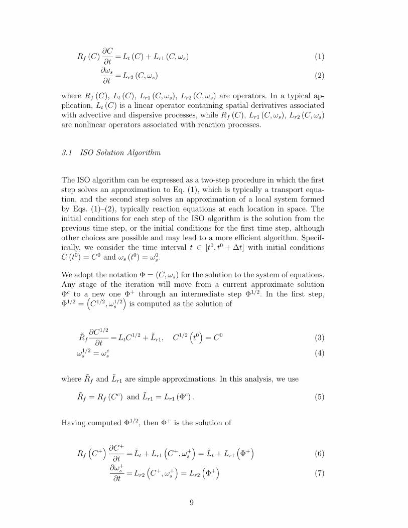
where Rf (C), Lt (C), Lr1 (C, ωs), Lr2 (C, ωs) are operators. In a typical ap-plication, Lt (C) is a linear operator containing spatial derivatives associatedwith advective and dispersive processes, while Rf (C), Lr1 (C, ωs), Lr2 (C, ωs)are nonlinear operators associated with reaction processes.

3.1 ISO Solution Algorithm

The ISO algorithm can be expressed as a two-step procedure in which the firststep solves an approximation to Eq. (1), which is typically a transport equa-tion, and the second step solves an approximation of a local system formedby Eqs. (1)–(2), typically reaction equations at each location in space. Theinitial conditions for each step of the ISO algorithm is the solution from theprevious time step, or the initial conditions for the first time step, althoughother choices are possible and may lead to a more efficient algorithm. Specif-ically, we consider the time interval t ∈ [t0, t0 + ∆t] with initial conditionsC (t0) = C0 and ωs (t0) = ω0

s .

We adopt the notation Φ = (C, ωs) for the solution to the system of equations.Any stage of the iteration will move from a current approximate solutionΦc to a new one Φ+ through an intermediate step Φ1/2. In the first step,Φ1/2 =

(

C1/2, ω1/2s

)

is computed as the solution of

Rf∂C1/2

∂t= LtC

1/2 + Lr1, C1/2(

t0)

= C0 (3)

ω1/2s = ωc

s (4)

where Rf and Lr1 are simple approximations. In this analysis, we use

Rf = Rf (Cc) and Lr1 = Lr1 (Φc) . (5)

Having computed Φ1/2, then Φ+ is the solution of

Rf

(

C+) ∂C+

∂t= Lt + Lr1

(

C+, ω+s

)

= Lt + Lr1

(

Φ+)

(6)

∂ω+s

∂t= Lr2

(

C+, ω+s

)

= Lr2

(

Φ+)

(7)

9

with initial condition Φ+ (t0) = (C0, ω0s). Here Lt is an approximation. In this

work, we use

Lt = LtC1/2. (8)

As long as the spatial discretization is fixed over the course of the ISO iter-ations, we can ignore the spatial variables because they have no role in theanalysis and the results will hold in one-dimensional (1D), two-dimensional(2D) and three-dimensional (3D) domains.

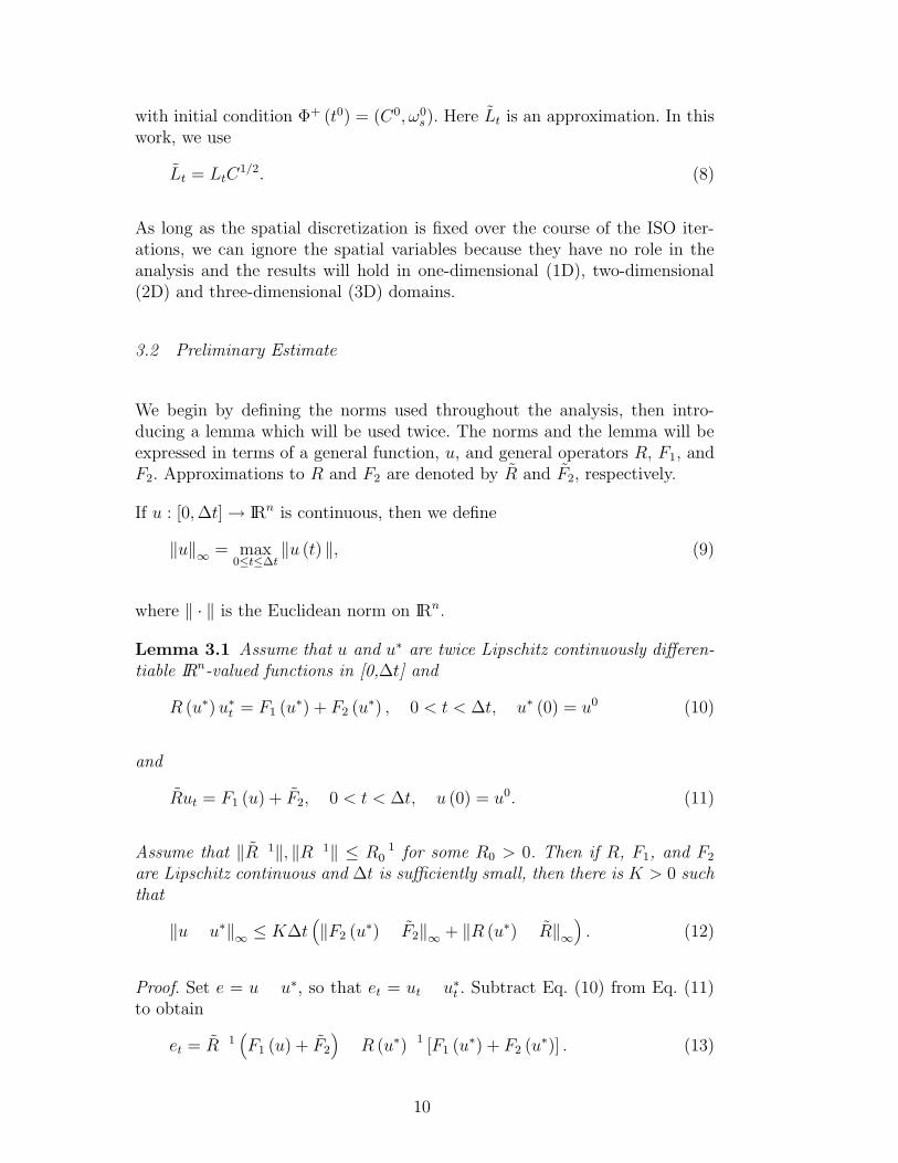
3.2 Preliminary Estimate

We begin by defining the norms used throughout the analysis, then intro-ducing a lemma which will be used twice. The norms and the lemma will beexpressed in terms of a general function, u, and general operators R, F1, andF2. Approximations to R and F2 are denoted by R and F2, respectively.

If u : [0, ∆t] → IRn is continuous, then we define

‖u‖∞

= max0≤t≤∆t

‖u (t) ‖, (9)

where ‖ · ‖ is the Euclidean norm on IRn.

Lemma 3.1 Assume that u and u∗ are twice Lipschitz continuously differen-tiable IRn-valued functions in [0,∆t] and

R (u∗) u∗t = F1 (u∗) + F2 (u∗) , 0 < t < ∆t, u∗ (0) = u0 (10)

and

Rut = F1 (u) + F2, 0 < t < ∆t, u (0) = u0. (11)

Assume that ‖R 1‖, ‖R 1‖ ≤ R 10 for some R0 > 0. Then if R, F1, and F2

are Lipschitz continuous and ∆t is sufficiently small, then there is K > 0 suchthat

‖u u∗‖∞

≤ K∆t(

‖F2 (u∗) F2‖∞ + ‖R (u∗) R‖∞

)

. (12)

Proof. Set e = u u∗, so that et = ut u∗t . Subtract Eq. (10) from Eq. (11)

to obtain

et = R 1(

F1 (u) + F2

)

R (u∗) 1 [F1 (u∗) + F2 (u∗)] . (13)

10

Adding and subtracting R 1 [F1 (u∗) + F2 (u∗)] and rearranging yields

et = R 1 [F1 (u) F1 (u∗)] +(

R 1 R (u∗) 1)

F1 (u∗)

+R 1[

F2 F2 (u∗)]

+(

R 1 R (u∗) 1)

F2 (u∗) .(14)

Combining the second and fourth terms in Eq. (14) yields

et = R 1 [F1 (u) F1 (u∗)] +R (u∗) R

RR (u∗)[F1 (u∗) + F2 (u∗)]

+R 1[

F2 F2 (u∗)]

.

(15)

Let γ1 be the Lipschitz constant of F1. By assumption∥

∥

∥ R 1 [F1 (u) F1 (u∗)]∥

∥

∥

∞≤ R 1

0 γ1‖e‖∞ , (16)

and therefore, letting

M = R 20 [ ‖F1 (u∗) ‖∞ + ‖F2 (u∗) ‖

∞] ‖R (u∗) R‖

∞

+R 10 ‖F2 (u∗) F2‖∞,

(17)

we have

‖et (t) ‖ ≤ R 10 γ1‖e‖∞ + M. (18)

Hence, for all 0 < t < ∆t,

‖e (t) ‖ =

∥

∥

∥

∥

∥

∥

t∫

0

et (s) ds

∥

∥

∥

∥

∥

∥

≤t

∫

0

[

R 10 γ1‖e‖∞ + M

]

ds. (19)

So,

‖e‖∞ ≤ ∆t(

R 10 γ1‖e‖∞ + M

)

. (20)

Assuming that 1 ∆tR 10 γ1 < 1/2 and setting

K = max(

R 20 (‖F1 (u∗) ‖∞ + ‖F2 (u∗) ‖∞) , R 1

0

)

(21)

completes the proof.

11

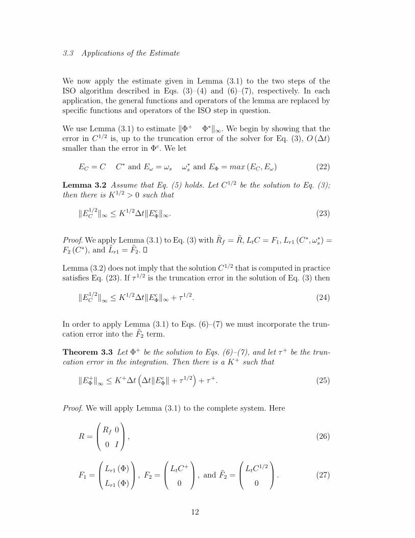
3.3 Applications of the Estimate

We now apply the estimate given in Lemma (3.1) to the two steps of theISO algorithm described in Eqs. (3)–(4) and (6)–(7), respectively. In eachapplication, the general functions and operators of the lemma are replaced byspecific functions and operators of the ISO step in question.

We use Lemma (3.1) to estimate ‖Φ+ Φ∗‖∞. We begin by showing that theerror in C1/2 is, up to the truncation error of the solver for Eq. (3), O (∆t)smaller than the error in Φc. We let

EC = C C∗ and Eω = ωs ω∗s and EΦ = max (EC , Eω) (22)

Lemma 3.2 Assume that Eq. (5) holds. Let C1/2 be the solution to Eq. (3);then there is K1/2 > 0 such that

‖E1/2C ‖∞ ≤ K1/2∆t‖Ec

Φ‖∞. (23)

Proof. We apply Lemma (3.1) to Eq. (3) with Rf = R, LtC = F1, Lr1 (C∗, ω∗s) =

F2 (C∗), and Lr1 = F2.

Lemma (3.2) does not imply that the solution C1/2 that is computed in practicesatisfies Eq. (23). If τ 1/2 is the truncation error in the solution of Eq. (3) then

‖E1/2C ‖

∞≤ K1/2∆t‖Ec

Φ‖∞ + τ 1/2. (24)

In order to apply Lemma (3.1) to Eqs. (6)–(7) we must incorporate the trun-cation error into the F2 term.

Theorem 3.3 Let Φ+ be the solution to Eqs. (6)–(7), and let τ+ be the trun-cation error in the integration. Then there is a K+ such that

‖E+Φ‖∞ ≤ K+∆t

(

∆t‖EcΦ‖ + τ 1/2

)

+ τ+. (25)

Proof. We will apply Lemma (3.1) to the complete system. Here

R =

Rf 0

0 I

, (26)

F1 =

Lr1 (Φ)

Lr1 (Φ)

, F2 =

LtC+

0

, and F2 =

LtC1/2

0

. (27)

12

The error in F2 does not depend on Eω, in fact

‖F2 (Φ∗) F2‖∞ ≤ M‖E1/2C ‖

∞≤ M

(

K1/2∆t‖EcC‖∞ + τ 1/2

)

. (28)

Eq. (25) follows directly from the lemma and Eq. (28).

As was the case with τ 1/2, τ+ reflects the truncation error of the solution. Tosummarize, Theorem 3.3 says that, within the truncation error of the solutionmethods, the error in Φ+ should be O(∆t2) smaller than the error in Φc.

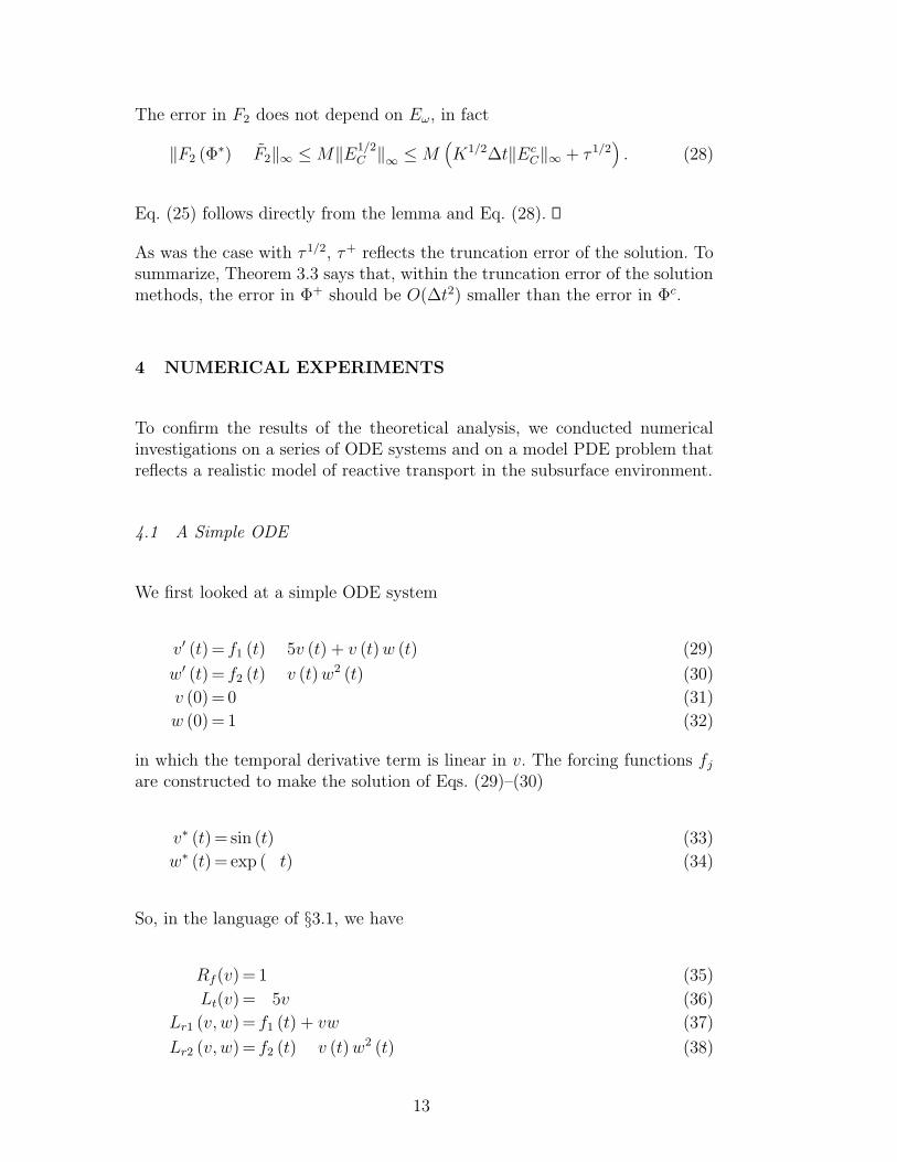
4 NUMERICAL EXPERIMENTS

To confirm the results of the theoretical analysis, we conducted numericalinvestigations on a series of ODE systems and on a model PDE problem thatreflects a realistic model of reactive transport in the subsurface environment.

4.1 A Simple ODE

We first looked at a simple ODE system

v′ (t) = f1 (t) 5v (t) + v (t) w (t) (29)

w′ (t) = f2 (t) v (t) w2 (t) (30)

v (0) = 0 (31)

w (0) = 1 (32)

in which the temporal derivative term is linear in v. The forcing functions fj

are constructed to make the solution of Eqs. (29)–(30)

v∗ (t) = sin (t) (33)

w∗ (t) = exp ( t) (34)

So, in the language of §3.1, we have

Rf (v) = 1 (35)

Lt(v) = 5v (36)

Lr1 (v, w) = f1 (t) + vw (37)

Lr2 (v, w) = f2 (t) v (t) w2 (t) (38)

13

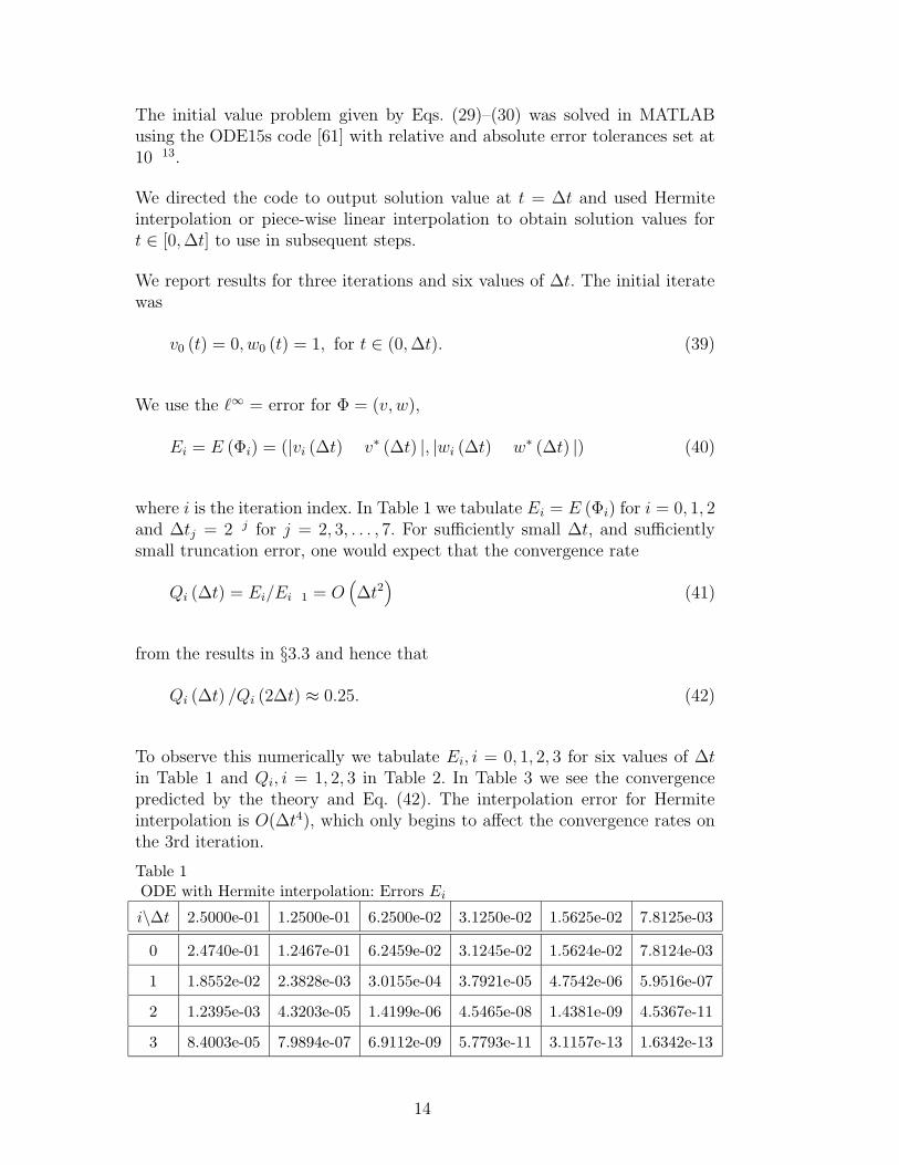
The initial value problem given by Eqs. (29)–(30) was solved in MATLABusing the ODE15s code [61] with relative and absolute error tolerances set at10 13.

We directed the code to output solution value at t = ∆t and used Hermiteinterpolation or piece-wise linear interpolation to obtain solution values fort ∈ [0, ∆t] to use in subsequent steps.

We report results for three iterations and six values of ∆t. The initial iteratewas

v0 (t) = 0, w0 (t) = 1, for t ∈ (0, ∆t). (39)

We use the `∞ = error for Φ = (v, w),

Ei = E (Φi) = (|vi (∆t) v∗ (∆t) |, |wi (∆t) w∗ (∆t) |) (40)

where i is the iteration index. In Table 1 we tabulate Ei = E (Φi) for i = 0, 1, 2and ∆tj = 2 j for j = 2, 3, . . . , 7. For sufficiently small ∆t, and sufficientlysmall truncation error, one would expect that the convergence rate

Qi (∆t) = Ei/Ei 1 = O(

∆t2)

(41)

from the results in §3.3 and hence that

Qi (∆t) /Qi (2∆t) ≈ 0.25. (42)

To observe this numerically we tabulate Ei, i = 0, 1, 2, 3 for six values of ∆tin Table 1 and Qi, i = 1, 2, 3 in Table 2. In Table 3 we see the convergencepredicted by the theory and Eq. (42). The interpolation error for Hermiteinterpolation is O(∆t4), which only begins to affect the convergence rates onthe 3rd iteration.

Table 1ODE with Hermite interpolation: Errors Ei

i\∆t 2.5000e-01 1.2500e-01 6.2500e-02 3.1250e-02 1.5625e-02 7.8125e-03

0 2.4740e-01 1.2467e-01 6.2459e-02 3.1245e-02 1.5624e-02 7.8124e-03

1 1.8552e-02 2.3828e-03 3.0155e-04 3.7921e-05 4.7542e-06 5.9516e-07

2 1.2395e-03 4.3203e-05 1.4199e-06 4.5465e-08 1.4381e-09 4.5367e-11

3 8.4003e-05 7.9894e-07 6.9112e-09 5.7793e-11 3.1157e-13 1.6342e-13

14

Table 2ODE with Hermite interpolation: Ratios Qi = Ei/Ei 1

i\∆t 2.5000e-01 1.2500e-01 6.2500e-02 3.1250e-02 1.5625e-02 7.8125e-03

1 7.4985e-02 1.9112e-02 4.8279e-03 1.2137e-03 3.0428e-04 7.6181e-05

2 6.6811e-02 1.8131e-02 4.7086e-03 1.1990e-03 3.0250e-04 7.6226e-05

3 6.7774e-02 1.8493e-02 4.8675e-03 1.2711e-03 2.1665e-04 3.6022e-03

Table 3ODE with Hermite interpolation: Estimated Rates Qi(∆t)/Qi(2∆t)

i\∆t 1.2500e-01 6.2500e-02 3.1250e-02 1.5625e-02 7.8125e-03

1 2.5488e-01 2.5261e-01 2.5138e-01 2.5072e-01 2.5036e-01

2 2.7138e-01 2.5970e-01 2.5463e-01 2.5230e-01 2.5199e-01

3 2.7286e-01 2.6321e-01 2.6115e-01 1.7044e-01 1.6627e+01

4.2 A Simple ODE With Errors

Here we repeat the computations from §4.1 under conditions more likely to bepresent in actual computations, i.e., the integration of the split equations andthe operator estimates contain error. We introduce several types of error by:(1) replacing Hermite interpolation with linear interpolation; (2) increasingthe tolerance of the ODE solver in both split equations; and (3) reducing theorder and the accuracy of only the transport solve. The effect of any of theseerrors will be to increase the truncation error effects in Eqs. (24) and (25) andmake Eq. (42) fail when the truncation error terms dominate the right sidesof Eqs. (24) and (25).

4.2.1 Interpolation Error

We repeat the computations in §4.1, except now we use linear interpolationto estimate Lr1 and Lt over the transport and reaction solves, respectively.The error in linear interpolation is O (∆t2), the same order as the reduction inerrors. As expected, we see interpolation effects in the second iteration, shownin the second row of Table 5.

4.2.2 Truncation Error

We also investigate the effect on the ISO convergence rate of increased trun-cation error in the ODE solver. We consider the case when both steps aresolved to the same tolerance, and also the case where one step is solved lessaccurately than the other.

15

Table 4ODE with linear interpolation: Errors Ei

i\∆t 2.5000e-01 1.2500e-01 6.2500e-02 3.1250e-02 1.5625e-02 7.8125e-03

0 2.4740e-01 1.2467e-01 6.2459e-02 3.1245e-02 1.5624e-02 7.8124e-03

1 1.2823e-02 1.9587e-03 2.7272e-04 3.6042e-05 4.6343e-06 5.8759e-07

2 2.7850e-04 2.3675e-05 2.0909e-06 1.6016e-07 1.1136e-08 7.3461e-10

3 8.7598e-04 5.3147e-05 3.2574e-06 2.0131e-07 1.2503e-08 7.7869e-10

Table 5ODE with linear interpolation: Estimated Rates Qi(∆t)/Qi(2∆t)

i\∆t 1.2500e-01 6.2500e-02 3.1250e-02 1.5625e-02 7.8125e-03

1 3.0312e-01 2.7793e-01 2.6418e-01 2.5713e-01 2.5357e-01

2 5.5652e-01 6.3427e-01 5.7962e-01 5.4074e-01 5.2029e-01

3 7.1370e-01 6.9401e-01 8.0680e-01 8.9329e-01 9.4407e-01

First we repeat the computations of §4.1 using atol = rtol = 10 4 in the ODEsolver ODE15s. The first row of Table 7 indicates that as (∆t) is reduced, thetruncation error will begin to dominate, and second-order convergence is notevident. The ratio Qi(∆t)/Qi(2∆t) actually increases as (∆t) is decreased.

Table 6ODE with solver tolerance = 10 4: Errors Ei

i\∆t 2.5000e-01 1.2500e-01 6.2500e-02 3.1250e-02 1.5625e-02 7.8125e-03

0 2.4740e-01 1.2467e-01 6.2459e-02 3.1245e-02 1.5624e-02 7.8124e-03

1 1.8148e-02 2.3925e-03 3.3655e-04 1.0494e-04 4.8641e-05 2.0856e-05

2 1.1167e-03 1.8007e-04 1.5880e-04 1.0582e-04 4.8756e-05 2.0866e-05

3 1.3209e-04 1.7829e-04 1.5875e-04 1.0582e-04 4.8756e-05 2.0866e-05

Table 7ODE with solver tolerance = 10 4: Estimated Rates Qi(∆t)/Qi(2∆t)

i\∆t 1.2500e-01 6.2500e-02 3.1250e-02 1.5625e-02 7.8125e-03

1 2.6161e-01 2.8079e-01 6.2335e-01 9.2687e-01 8.5751e-01

2 1.2232e+00 6.2691e+00 2.1369e+00 9.9410e-01 9.9814e-01

3 8.3700e+00 1.0097e+00 1.0003e+00 1.0000e+00 1.0000e+00

Fully coupled solutions to NRTP’s are typically implemented using low-orderfinite difference or finite element methods which are second-order accuratein space and time. Although typical ISO implementations solve the reactionstep using methods which are higher order in time, the transport step is oftensolved using methods that are lower order in time and often use fixed time

16

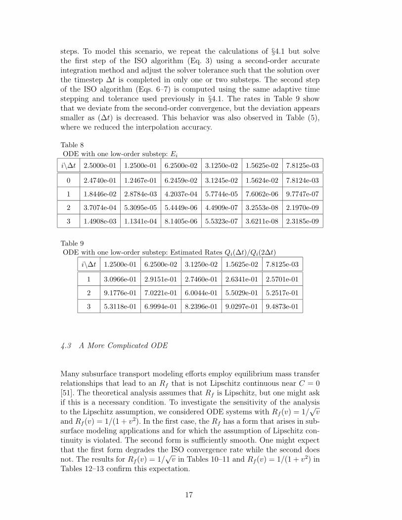
steps. To model this scenario, we repeat the calculations of §4.1 but solvethe first step of the ISO algorithm (Eq. 3) using a second-order accurateintegration method and adjust the solver tolerance such that the solution overthe timestep ∆t is completed in only one or two substeps. The second stepof the ISO algorithm (Eqs. 6–7) is computed using the same adaptive timestepping and tolerance used previously in §4.1. The rates in Table 9 showthat we deviate from the second-order convergence, but the deviation appearssmaller as (∆t) is decreased. This behavior was also observed in Table (5),where we reduced the interpolation accuracy.

Table 8ODE with one low-order substep: Ei

i\∆t 2.5000e-01 1.2500e-01 6.2500e-02 3.1250e-02 1.5625e-02 7.8125e-03

0 2.4740e-01 1.2467e-01 6.2459e-02 3.1245e-02 1.5624e-02 7.8124e-03

1 1.8446e-02 2.8784e-03 4.2037e-04 5.7744e-05 7.6062e-06 9.7747e-07

2 3.7074e-04 5.3095e-05 5.4449e-06 4.4909e-07 3.2553e-08 2.1970e-09

3 1.4908e-03 1.1341e-04 8.1405e-06 5.5323e-07 3.6211e-08 2.3185e-09

Table 9ODE with one low-order substep: Estimated Rates Qi(∆t)/Qi(2∆t)

i\∆t 1.2500e-01 6.2500e-02 3.1250e-02 1.5625e-02 7.8125e-03

1 3.0966e-01 2.9151e-01 2.7460e-01 2.6341e-01 2.5701e-01

2 9.1776e-01 7.0221e-01 6.0044e-01 5.5029e-01 5.2517e-01

3 5.3118e-01 6.9994e-01 8.2396e-01 9.0297e-01 9.4873e-01

4.3 A More Complicated ODE

Many subsurface transport modeling efforts employ equilibrium mass transferrelationships that lead to an Rf that is not Lipschitz continuous near C = 0[51]. The theoretical analysis assumes that Rf is Lipschitz, but one might askif this is a necessary condition. To investigate the sensitivity of the analysisto the Lipschitz assumption, we considered ODE systems with Rf (v) = 1/

√v

and Rf (v) = 1/(1 + v2). In the first case, the Rf has a form that arises in sub-surface modeling applications and for which the assumption of Lipschitz con-tinuity is violated. The second form is sufficiently smooth. One might expectthat the first form degrades the ISO convergence rate while the second doesnot. The results for Rf (v) = 1/

√v in Tables 10–11 and Rf (v) = 1/(1 + v2) in

Tables 12–13 confirm this expectation.

17

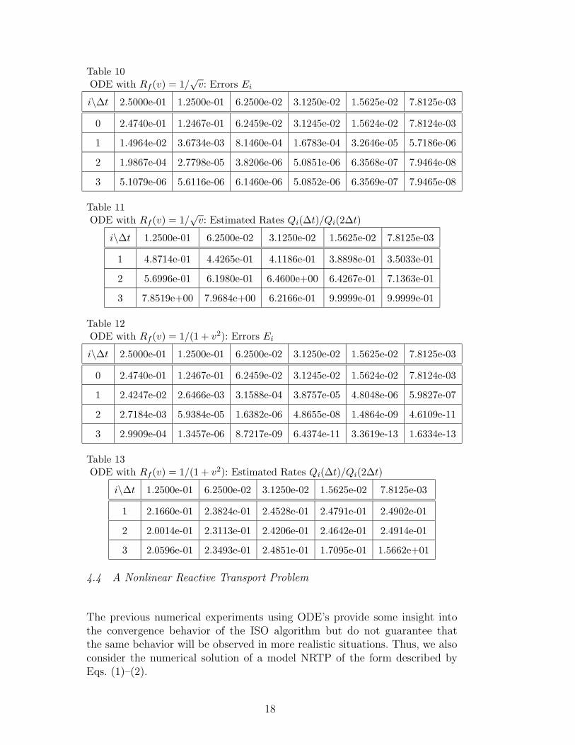
Table 10ODE with Rf (v) = 1/

√v: Errors Ei

i\∆t 2.5000e-01 1.2500e-01 6.2500e-02 3.1250e-02 1.5625e-02 7.8125e-03

0 2.4740e-01 1.2467e-01 6.2459e-02 3.1245e-02 1.5624e-02 7.8124e-03

1 1.4964e-02 3.6734e-03 8.1460e-04 1.6783e-04 3.2646e-05 5.7186e-06

2 1.9867e-04 2.7798e-05 3.8206e-06 5.0851e-06 6.3568e-07 7.9464e-08

3 5.1079e-06 5.6116e-06 6.1460e-06 5.0852e-06 6.3569e-07 7.9465e-08

Table 11ODE with Rf (v) = 1/

√v: Estimated Rates Qi(∆t)/Qi(2∆t)

i\∆t 1.2500e-01 6.2500e-02 3.1250e-02 1.5625e-02 7.8125e-03

1 4.8714e-01 4.4265e-01 4.1186e-01 3.8898e-01 3.5033e-01

2 5.6996e-01 6.1980e-01 6.4600e+00 6.4267e-01 7.1363e-01

3 7.8519e+00 7.9684e+00 6.2166e-01 9.9999e-01 9.9999e-01

Table 12ODE with Rf (v) = 1/(1 + v2): Errors Ei

i\∆t 2.5000e-01 1.2500e-01 6.2500e-02 3.1250e-02 1.5625e-02 7.8125e-03

0 2.4740e-01 1.2467e-01 6.2459e-02 3.1245e-02 1.5624e-02 7.8124e-03

1 2.4247e-02 2.6466e-03 3.1588e-04 3.8757e-05 4.8048e-06 5.9827e-07

2 2.7184e-03 5.9384e-05 1.6382e-06 4.8655e-08 1.4864e-09 4.6109e-11

3 2.9909e-04 1.3457e-06 8.7217e-09 6.4374e-11 3.3619e-13 1.6334e-13

Table 13ODE with Rf (v) = 1/(1 + v2): Estimated Rates Qi(∆t)/Qi(2∆t)

i\∆t 1.2500e-01 6.2500e-02 3.1250e-02 1.5625e-02 7.8125e-03

1 2.1660e-01 2.3824e-01 2.4528e-01 2.4791e-01 2.4902e-01

2 2.0014e-01 2.3113e-01 2.4206e-01 2.4642e-01 2.4914e-01

3 2.0596e-01 2.3493e-01 2.4851e-01 1.7095e-01 1.5662e+01

4.4 A Nonlinear Reactive Transport Problem

The previous numerical experiments using ODE’s provide some insight intothe convergence behavior of the ISO algorithm but do not guarantee thatthe same behavior will be observed in more realistic situations. Thus, we alsoconsider the numerical solution of a model NRTP of the form described byEqs. (1)–(2).

18

4.4.1 Model Formulation

For convenience, we consider a model problem introduced in [29], which de-scribes solute transport, reaction, and interphase mass transfer in a porousmedium system. Mass transfer occurs between a fluid phase and two types ofsolid phase—a fraction that achieves equilibrium quickly and a fraction thatachieves equilibrium slowly. Transformation reactions are considered to be ofa general form and may be linear or nonlinear. Subsets of this general modeloccur routinely in application, and because of this it makes a good test prob-lem for the solution issues of concern in this work. Because the major aspectsof this work do not depend upon the spatial dimensionality of the system, wewill restrict our efforts to one spatial dimension. We also limit ourselves to thecase of transport with a known uniform flow field. This subset of the governingequations describing 1D transport in a uniform flow field is often employedfor problems such as solute transport through soil columns, e.g. [17, 38, 20],fixed bed reactors, e.g. [3, 34, 46], and in many field-scale investigations, e.g.[1, 55, 60].

We formulate this model as

∂C

∂t+

ρb

θ

∂ωf

∂t= Dx

∂2C

∂x2 vx

∂C

∂x kaC

ra (43)

ρb

θ

[

α (ωes ωs) + kfω

rf

f

]

, in [0, Lx] × [0, ts]

∂ωs

∂t= α (ωe

s ωs) ksωrs

s , in [0, Lx] × [0, ts] (44)

subject to boundary conditions

C (0, t) = C0 (45)

∂C

∂x(Lx, t) = 0 (46)

and initial conditions

C (x, 0) = sin(

πx

Lx

)

(47)

ωs (x, 0) = 0 (48)

where [0, Lx] ⊂ IR1 is the spatial domain; [0, ts] is the temporal domain; x andt are the spatial and temporal coordinates, respectively; C is an aqueous phasesolute concentration; t is time; Dx is a hydrodynamic dispersion coefficient;vx is a mean pore velocity; ka, kf , and ks are reaction rate constants for theaqueous-phase, the rapidly sorbing solid phase, and the slowly sorbing solid

19

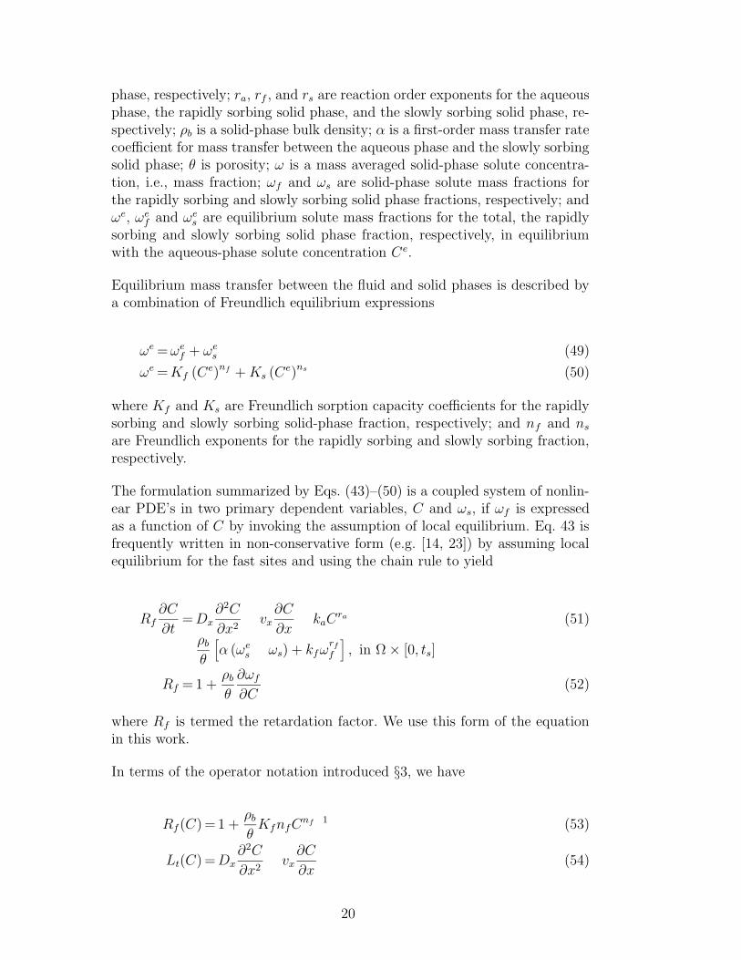
phase, respectively; ra, rf , and rs are reaction order exponents for the aqueousphase, the rapidly sorbing solid phase, and the slowly sorbing solid phase, re-spectively; ρb is a solid-phase bulk density; α is a first-order mass transfer ratecoefficient for mass transfer between the aqueous phase and the slowly sorbingsolid phase; θ is porosity; ω is a mass averaged solid-phase solute concentra-tion, i.e., mass fraction; ωf and ωs are solid-phase solute mass fractions forthe rapidly sorbing and slowly sorbing solid phase fractions, respectively; andωe, ωe

f and ωes are equilibrium solute mass fractions for the total, the rapidly

sorbing and slowly sorbing solid phase fraction, respectively, in equilibriumwith the aqueous-phase solute concentration Ce.

Equilibrium mass transfer between the fluid and solid phases is described bya combination of Freundlich equilibrium expressions

ωe = ωef + ωe

s (49)

ωe = Kf (Ce)nf + Ks (Ce)ns (50)

where Kf and Ks are Freundlich sorption capacity coefficients for the rapidlysorbing and slowly sorbing solid-phase fraction, respectively; and nf and ns

are Freundlich exponents for the rapidly sorbing and slowly sorbing fraction,respectively.

The formulation summarized by Eqs. (43)–(50) is a coupled system of nonlin-ear PDE’s in two primary dependent variables, C and ωs, if ωf is expressedas a function of C by invoking the assumption of local equilibrium. Eq. 43 isfrequently written in non-conservative form (e.g. [14, 23]) by assuming localequilibrium for the fast sites and using the chain rule to yield

Rf∂C

∂t= Dx

∂2C

∂x2 vx

∂C

∂x kaC

ra (51)

ρb

θ

[

α (ωes ωs) + kfω

rf

f

]

, in Ω × [0, ts]

Rf = 1 +ρb

θ

∂ωf

∂C(52)

where Rf is termed the retardation factor. We use this form of the equationin this work.

In terms of the operator notation introduced §3, we have

Rf (C) = 1 +ρb

θKfnfC

nf 1 (53)

Lt(C) = Dx∂2C

∂x2 vx

∂C

∂x(54)

20

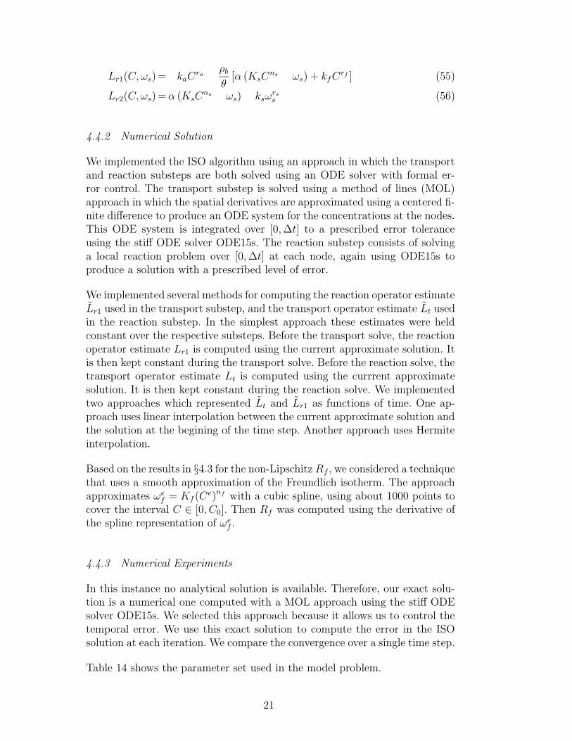
Lr1(C, ωs) = kaCra ρb

θ[α (KsC

ns ωs) + kfCrf ] (55)

Lr2(C, ωs) = α (KsCns ωs) ksω

rs

s (56)

4.4.2 Numerical Solution

We implemented the ISO algorithm using an approach in which the transportand reaction substeps are both solved using an ODE solver with formal er-ror control. The transport substep is solved using a method of lines (MOL)approach in which the spatial derivatives are approximated using a centered fi-nite difference to produce an ODE system for the concentrations at the nodes.This ODE system is integrated over [0, ∆t] to a prescribed error toleranceusing the stiff ODE solver ODE15s. The reaction substep consists of solvinga local reaction problem over [0, ∆t] at each node, again using ODE15s toproduce a solution with a prescribed level of error.

We implemented several methods for computing the reaction operator estimateLr1 used in the transport substep, and the transport operator estimate Lt usedin the reaction substep. In the simplest approach these estimates were heldconstant over the respective substeps. Before the transport solve, the reactionoperator estimate Lr1 is computed using the current approximate solution. Itis then kept constant during the transport solve. Before the reaction solve, thetransport operator estimate Lt is computed using the currrent approximatesolution. It is then kept constant during the reaction solve. We implementedtwo approaches which represented Lt and Lr1 as functions of time. One ap-proach uses linear interpolation between the current approximate solution andthe solution at the begining of the time step. Another approach uses Hermiteinterpolation.

Based on the results in §4.3 for the non-Lipschitz Rf , we considered a techniquethat uses a smooth approximation of the Freundlich isotherm. The approachapproximates ωe

f = Kf (Ce)nf with a cubic spline, using about 1000 points to

cover the interval C ∈ [0, C0]. Then Rf was computed using the derivative ofthe spline representation of ωe

f .

4.4.3 Numerical Experiments

In this instance no analytical solution is available. Therefore, our exact solu-tion is a numerical one computed with a MOL approach using the stiff ODEsolver ODE15s. We selected this approach because it allows us to control thetemporal error. We use this exact solution to compute the error in the ISOsolution at each iteration. We compare the convergence over a single time step.

Table 14 shows the parameter set used in the model problem.

21

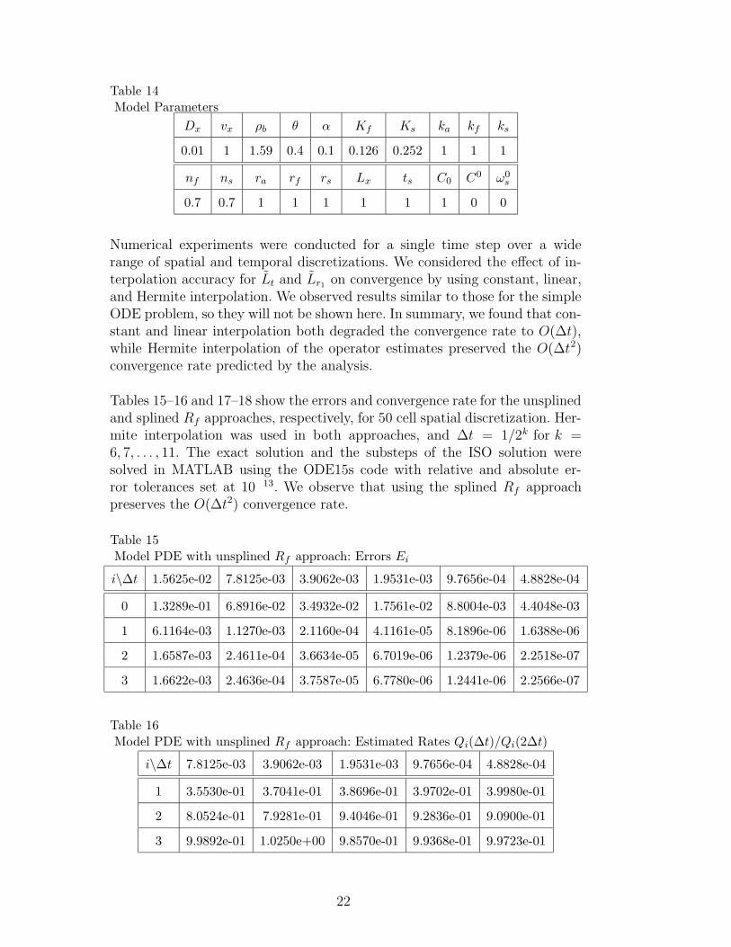
Table 14Model Parameters

Dx vx ρb θ α Kf Ks ka kf ks

0.01 1 1.59 0.4 0.1 0.126 0.252 1 1 1

nf ns ra rf rs Lx ts C0 C0 ω0s

0.7 0.7 1 1 1 1 1 1 0 0

Numerical experiments were conducted for a single time step over a widerange of spatial and temporal discretizations. We considered the effect of in-terpolation accuracy for Lt and Lr1

on convergence by using constant, linear,and Hermite interpolation. We observed results similar to those for the simpleODE problem, so they will not be shown here. In summary, we found that con-stant and linear interpolation both degraded the convergence rate to O(∆t),while Hermite interpolation of the operator estimates preserved the O(∆t2)convergence rate predicted by the analysis.

Tables 15–16 and 17–18 show the errors and convergence rate for the unsplinedand splined Rf approaches, respectively, for 50 cell spatial discretization. Her-mite interpolation was used in both approaches, and ∆t = 1/2k for k =6, 7, . . . , 11. The exact solution and the substeps of the ISO solution weresolved in MATLAB using the ODE15s code with relative and absolute er-ror tolerances set at 10 13. We observe that using the splined Rf approachpreserves the O(∆t2) convergence rate.

Table 15Model PDE with unsplined Rf approach: Errors Ei

i\∆t 1.5625e-02 7.8125e-03 3.9062e-03 1.9531e-03 9.7656e-04 4.8828e-04

0 1.3289e-01 6.8916e-02 3.4932e-02 1.7561e-02 8.8004e-03 4.4048e-03

1 6.1164e-03 1.1270e-03 2.1160e-04 4.1161e-05 8.1896e-06 1.6388e-06

2 1.6587e-03 2.4611e-04 3.6634e-05 6.7019e-06 1.2379e-06 2.2518e-07

3 1.6622e-03 2.4636e-04 3.7587e-05 6.7780e-06 1.2441e-06 2.2566e-07

Table 16Model PDE with unsplined Rf approach: Estimated Rates Qi(∆t)/Qi(2∆t)

i\∆t 7.8125e-03 3.9062e-03 1.9531e-03 9.7656e-04 4.8828e-04

1 3.5530e-01 3.7041e-01 3.8696e-01 3.9702e-01 3.9980e-01

2 8.0524e-01 7.9281e-01 9.4046e-01 9.2836e-01 9.0900e-01

3 9.9892e-01 1.0250e+00 9.8570e-01 9.9368e-01 9.9723e-01

22

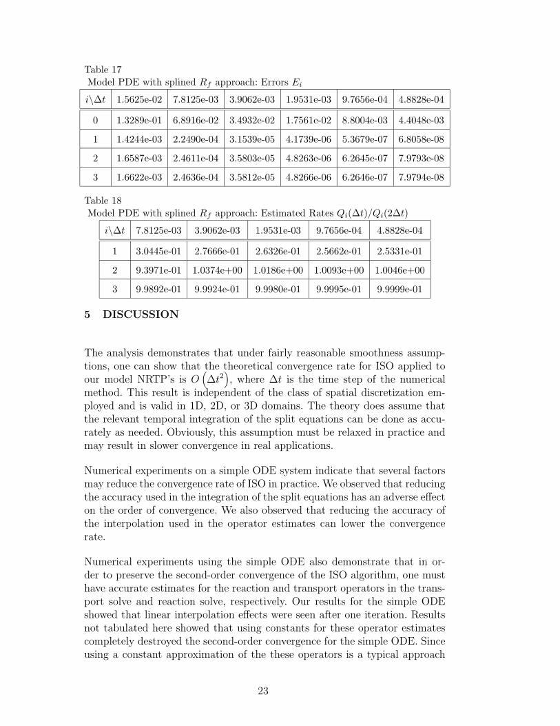
Table 17Model PDE with splined Rf approach: Errors Ei

i\∆t 1.5625e-02 7.8125e-03 3.9062e-03 1.9531e-03 9.7656e-04 4.8828e-04

0 1.3289e-01 6.8916e-02 3.4932e-02 1.7561e-02 8.8004e-03 4.4048e-03

1 1.4244e-03 2.2490e-04 3.1539e-05 4.1739e-06 5.3679e-07 6.8058e-08

2 1.6587e-03 2.4611e-04 3.5803e-05 4.8263e-06 6.2645e-07 7.9793e-08

3 1.6622e-03 2.4636e-04 3.5812e-05 4.8266e-06 6.2646e-07 7.9794e-08

Table 18Model PDE with splined Rf approach: Estimated Rates Qi(∆t)/Qi(2∆t)

i\∆t 7.8125e-03 3.9062e-03 1.9531e-03 9.7656e-04 4.8828e-04

1 3.0445e-01 2.7666e-01 2.6326e-01 2.5662e-01 2.5331e-01

2 9.3971e-01 1.0374e+00 1.0186e+00 1.0093e+00 1.0046e+00

3 9.9892e-01 9.9924e-01 9.9980e-01 9.9995e-01 9.9999e-01

5 DISCUSSION

The analysis demonstrates that under fairly reasonable smoothness assump-tions, one can show that the theoretical convergence rate for ISO applied toour model NRTP’s is O

(

∆t2)

, where ∆t is the time step of the numericalmethod. This result is independent of the class of spatial discretization em-ployed and is valid in 1D, 2D, or 3D domains. The theory does assume thatthe relevant temporal integration of the split equations can be done as accu-rately as needed. Obviously, this assumption must be relaxed in practice andmay result in slower convergence in real applications.

Numerical experiments on a simple ODE system indicate that several factorsmay reduce the convergence rate of ISO in practice. We observed that reducingthe accuracy used in the integration of the split equations has an adverse effecton the order of convergence. We also observed that reducing the accuracy ofthe interpolation used in the operator estimates can lower the convergencerate.

Numerical experiments using the simple ODE also demonstrate that in or-der to preserve the second-order convergence of the ISO algorithm, one musthave accurate estimates for the reaction and transport operators in the trans-port solve and reaction solve, respectively. Our results for the simple ODEshowed that linear interpolation effects were seen after one iteration. Resultsnot tabulated here showed that using constants for these operator estimatescompletely destroyed the second-order convergence for the simple ODE. Sinceusing a constant approximation of the these operators is a typical approach

23

[42, 59, 71], it has significant implications for solving realistic problems.

Numerical experiments using an ODE with a model Rf term lend insightinto the importance of the Lipschitz continuity assumption used in the anal-ysis. The analysis treats Lipschitz continuity as a sufficient condition, but thenumerical experiments indicate that it may be a necessary condition. Thishas significant practical implications for subsurface transport investigations,since the Freundlich model for sorption equilibrium often used in subsurfacetransport simulations results in an Rf which is non-Lipschitz for very lowconcentrations. The Freundlich model does not reduce to a linear relationshipbetween C and ω at low fluid-phase concentrations. Instead, ∂ω/∂C tends toinfinity as the fluid phase solute concentration approaches zero.

The results of the numerical experiments on the model NRTP show that onecan implement the ISO algorithm in a manner that preserves the second-orderconvergence predicted by the theory. Simple constant or linear approximationsfor the transport and reaction operator estimates destroy the second-orderconvergence rate, while Hermite interpolation along with a smooth approxi-mation for the retardation factor preserve second-order convergence. We stressthat we looked at convergence, and we have not systematically investigatedthe computational efficiency of this approach. If the work for each iterationof the ISO method is excessive, it may not be competitive with other SOapproaches or with the best FC approaches. This is an area which deservesfurther research.

6 CONCLUSIONS

Based upon the analysis and numerical experiments, We draw several conclu-sions regarding the use of the ISO algorithm for NRTP’s:

(1) Theoretical analysis shows that, given certain assumptions regarding smooth-ness, the rate of convergence for ISO solution of NRTP’s is O(∆t2).

(2) Numerical experiments using a simple ODE system indicate that the the-oretical convergence rate can be degraded by discretization errors intro-duced into the numerical solution and by coarse estimates of the reactionand transport operators. Experiments on ODE models also imply thatLipschitz continuity is an important assumption in practice.

(3) Numerical experiments on a model PDE system using typical finite dif-ference implementations of the ISO approach (i.e., with constant andlinear estimates of the reaction and transport operators) and using theFreundlich sorption equilibrium model agree with the results of ODEexperiments.

(4) Our results show that by using Hermite interpolation to compute the

24

transport and reaction operator estimates, and using a smooth approxi-mation to the Freundlich sorption model, one can obtain the theoreticalrate of convergence.

(5) Additional research on the computational efficiency of the the ISO ap-proach introduced here is needed before it is proposed for routine sub-surface simulation projects.

Acknowledgements

The UNC aspects of this work have been supported by the National Instituteof Environmental Health Sciences (NIEHS) grant 5 P42 ES05948-02 and theNational Science Foundation (NSF) grant DMS-0112653. The work at NCSUhas been supported by NSF grants DMS-0070641 and DMS-0112542, and theUS Army Research Office (ARO) grant DAAD19-99-1-0186. Computationalsupport was provided by the North Carolina Supercomputer Center and fromCray Research, Inc.

References

[1] R.H. Abrams and K. Loague. A compartmentalized solute transportmodel for redox zones in contaminated aquifers, 2. Field-scale simulations.Water Resources Research, 36(8):2015–2029, 2000.

[2] C. A. J. Appelo and A. Willemsen. Geochemical calculations and obser-vations on salt water intrusions, I. A combined geochemical/mixing cellmodel. Journal of Hydrology, 94:313–330, 1987.

[3] A. K. Avci, D. L. Trimm, and Z. I. Onsan. Heterogeneous reactor model-ing for simulation of catalytic oxidation and steam reforming of methane.Chemical Engineering Science, 56(2):641–649, 2001.

[4] D. A. Barry. Supercomputers and their use in modeling subsurface solutetransport. Reviews of Geophysics, 38(3):277–295, 1990.

[5] D. A. Barry, C. T. Miller, P. J. Culligan, and K. Bajracharya. Splitoperator methods for reactive chemical transport in groundwater. InProceeding of the International Conference on Modeling and Simulation1995: MODSIM95, pages 125–132, New South Wales, 1995. Modeling andSimulation Society of Australia, Inc.

[6] D. A. Barry, C. T. Miller, P. J. Culligan, and K. Bajracharya. Analysisof split operator methods for nonlinear and multispecies groundwaterchemical transport models. Mathematics and Computers in Simulation,43:331–341, 1997.

[7] D. A. Barry, C. T. Miller, and P. J. Culligan-Hensley. Temporal discretiza-tion errors in non-iterative split-operator approaches to solving chemical

25

reaction/groundwater transport models. Journal of Contaminant Hydrol-ogy, 22(1/2):1–17, 1996.

[8] D.A. Barry, K. Bajracharya, M. Crapper, H. Prommer, and C.J. Cunning-ham. Comparison of split-operator methods for solving coupled chemicalnon-equilibrium reaction/groundwater transport models. Mathematicsand Computers in Simulation, 53:113–127, 2000.

[9] I. Bey, D.J. Jacob, R.M. Yantosca, J.A. Logan, B.D. Field, A.M. Fiore,Q.B. Li, H.G.Y. Liu, L.J. Mickley, and M.G. Schultz. Global modeling oftropospheric chemistry with assimilated meteorology: Model descriptionand evaluation. Journal of Geophysical Research-Atmospheres, 106(D19):23073–3095, 2001.

[10] D. Bhuyan, L. W. Lake, and G. A. Pope. Mathematical modeling ofhigh-pH chemical flooding. SPE Reservoir Engineering, 5:213–220, 1990.

[11] J.G. Blom and J.G. Verwer. A comparison of integration methods foratmospheric transport-chemistry problems. Journal of Computationaland Applied Mathematics, 126(1–2):381–396, 2000.

[12] M. Blunt, F. J. Fayers, and F. M. Orr. Carbon-dioxide in enhanced oil-recovery. Energy Conversion and Management, 34(9–1):1197–1204, 1992.

[13] R. C. Borden, P. B. Bedient, M. D. Lee, C. H. Ward, and J. T. Wil-son. Transport of dissolved hydrocarbons influenced by oxygen-limitedbiodegradation, 2. Field application. Water Resources Research, 22(13):1983–1990, 1986.

[14] M. L. Brusseau and P. S. C. Rao. Sorption nonideality during organic con-taminant transport in porous media. Critical Reviews in EnvironmentalControl, 19(1):33–99, 1989.

[15] M. A. Celia, J. S. Kindred, and I. Herrera. Contaminant transport andbiodegradation 1. A numerical model for reactive transport in porousmedia. Water Resources Research, 25(6):1141–1148, 1989.

[16] H. P. Cheng and G. T. Yeh. Development and demonstrative applicationof a 3-D numerical model of subsurface flow, heat transfer, and reactivechemical transport: 3DHYDROGEOCHEM. Journal of Contaminant Hy-drology, 34(1–2):47–83, 1998.

[17] C. V. Chrysikopoulos, P. K. Kitanidis, and P. V. Roberts. Analysis ofone-dimensional solute transport through porous media with spatiallyvariable retardation factor. Water Resources Research, 26(3):437–446,1990.

[18] S.P. Chu and H. Elliott. Latitude versus depth simulations of ecodynamicsand dissolved gas chemistry relationships in the central pacific. Journalof Atmospheric Chemistry, 40(3):305–333, 2001.

[19] D.M. Cooper, A. Jenkins, R. Skeffington, and B. Gannon. Catchment-scale simulation of stream water chemistry by spatial mixing: Theory andapplication. Journal of Hydrology, 233(1–4):4121–137, 2000.

[20] B. B. Dykaar and P. K. Kitanidis. Macrotransport of a biologically re-acting solute through porous media. Water Resources Research, 32(2):307–320, 1996.

26

[21] P. Engesgaard and K. L. Kipp. A geochemical transport model for redox-controlled movement of mineral fronts in groundwater flow systems — Acase of nitrate removal by oxidation of pyrite. Water Resources Research,28(10):2829–2843, 1992.

[22] P. Engesgaard and R. Traberg. Contaminant transport at a waste residuedeposit. 2. Geochemical transport modeling. Water Resources Research,32(4):939–951, 1996.

[23] T. C. Harmon, W. P. Ball, and P. V. Roberts. Nonequilibrium transport oforganic contaminants in groundwater. In B. L. Sawhney and K. Brown,editors, Reactions and Movement of Organic Chemicals in Soils, pages405–438. Soil Science Society of America, Inc., Madison, Wisconsin, 1989.

[24] J. Herzer and W. Kinzelbach. Coupling of transport and chemical pro-cesses in numerical transport models. Geoderma, 44:115–127, 1989.

[25] K.S. Hunter, Y.F. Wang, and P.M. Van Cappellen. Kinetic modeling ofmicrobially-driven redox chemistry of subsurface environments: Couplingtransport, microbial metabolism and geochemistry. Journal of Hydrology,209(1–4):53–80, 1998.

[26] M.Z. Jacobson. Fundamentals of Atmospheric Modeling. Cambridge Uni-versity Press, 1998.

[27] A. A. Jennings, D. J. Kirkner, and T. L. Theis. Multicomponent equi-librium chemistry in groundwater quality models. Water Resources Re-search, 18(4):1089–1096, 1982.

[28] J. J. Kaluarachchi and J. Morshed. Critical assessment of the operatorsplitting technique in solving the advection dispersion reaction equation.1. First-order reaction. Advances in Water Resources, 18(2):89–100, 1995.

[29] J. F. Kanney, C. T. Miller, and D. A. Barry. Comparison of fully coupledapproaches for approximating nonlinear transport and reaction problems.Advances in Water Resources, (In Press), 2002.

[30] J. Kim and S. Y. Cho. Computation accuracy and efficiency of the time-splitting method in solving atmospheric transport-chemistry equations.Atmospheric Environment, 31(15):2215–2224, 1997.

[31] A.A. Koelmans, A. Van der Heijde, L.M Knijff, and R.H. Aalderink. In-tegrated modelling of eutrophication and organic contaminant fate & ef-fects in aquatic ecosystems. A review. Water Research, 35(15):3517–3536,2001.

[32] R. Kopmann and Markofsky M. Three-dimensional water quality mod-elling with TELEMAC-3D. Hydrological Processes, 14(13):2279–2292,2000.

[33] A.S. Koziol and J.A. Pudykiewicz. Global-scale environmental transportof persistent organic pollutants. Chemosphere, 45(8):1181–1200, 2001.

[34] S. Krishnaswamy, R.D. Gunn, and P.K. Agarwal. Low-temperature ox-idation of coal, 2. An experimental and modelling investigation using afixed-bed isothermal flow reactor. Fuel, 75(3):344–352, 1996.

[35] L. W. Lake. Enhanced Oil Recovery. Prentice Hall, Englewood Cliffs, NJ,1989.

27

[36] D. Lanser and Verwer J.G. Analysis of operator splitting for advection-diffusion-reaction problems from air pollution modelling. Journal of Com-putational and Applied Mathematics, 111(1–2):201–216, 1999.

[37] R. J. LeVeque and J. Oliger. Numerical methods based on additive split-tings for hyperbolic partial differential equations. Mathematics of Com-putation, 40(162):469–497, 1983.

[38] D. M. Linn. Sorption and Degradation of Pesticides and Organic Chem-icals in Soil. Soil Science Society of America, Inc., and American Societyof Agronomy, Inc., Madison, WI, 1993.

[39] C. W. Liu and T. N. Narasimhan. Redox-controlled multiple-species reac-tive chemical transport 1. Model development. Water Resources Research,25(5):869–882, 1989.

[40] K. T. MacQuarrie, E. A. Sudicky, and E. O. Frind. Simulation ofbiodegradable organic contaminants in groundwater, 1. Numerical formu-lation in principal directions. Water Resources Research, 26(2):207–222,1990.

[41] A. Mahadevan and D. Archer. Modeling the impact of fronts andmesoscale circulation on the nutrient supply and biogeochemistry of theupper ocean. Journal of Geophysical Research-Oceans, 105(C1):1209–1225, 2000.

[42] W. W. Mcnab and T. N. Narasimhan. A multiple species transport modelwith sequential decay chain interactions in heterogeneous subsurface en-vironments. Water Resources Research, 29(8):2737–2746, 1993.

[43] G. J. McRae, W. R. Goodin, and J. H. Seinfeld. Numerical solution ofthe atmospheric diffusion equation for chemically reacting flows. Journalof Computational Physics, 45:1–42, 1982.

[44] C. T. Miller, G. Christakos, P. T. Imhoff, J. F. McBride, J. A. Pedit, andJ. A. Trangenstein. Multiphase flow and transport modeling in hetero-geneous porous media: Challenges and approaches. Advances in WaterResources, 21(2):77–120, 1998.

[45] C. T. Miller and A. J. Rabideau. Development of split-operator, Petrov-Galerkin methods to simulate transport and diffusion problems. WaterResources Research, 29(7):2227–2240, 1993.

[46] P. Mizsey, A. Cuellar, E. Newson, P. Hottinger, T. Truong, and F. vonRoth. Fixed bed reactor modelling and experimental data for catalyticdehydrogenation in seasonal energy storage applications. Computers &Chemical Engineering, 23:S379–S382, 1999.

[47] J. Morshed and J. J. Kaluarachchi. Critical assessment of the operatorsplitting technique in solving the advection dispersion reaction equation2. Monod kinetics and coupled transport. Advances in Water Resources,18(2):101–110, 1995.

[48] D.J. Mossman and N. AlMulki. One-dimensional unsteady flow and un-steady pesticide transport in a reservoir. Ecological Modelling, 89(1–3):259–267, 1996.

[49] E. S. Oran and J. P. Boris. Numerical Simulation of Reactive Flow.

28

Elsevier, New York, 1987.[50] D.L. Parkhurst. User’s Guide to PHREEQC: A Computer Program for

Speciation, Reaction-Path, Advective-Transport and Diffusion Problems.U.S. Geological Survey, 1995. Water Resource Investigation Report 95-4227.

[51] J. A. Pedit. An investigation of heterogeneous sorption by a natural solid.PhD thesis, University of North Carolina, Chapel Hill, NC, 1994.

[52] G. A. Pope and M. Baviere. Basic Concepts in Enhanced Oil RecoveryProcesses. Elsevier, New York, 1991.

[53] H. Prommer, D. A. Barry, and G. B. Davis. A one-dimensional reactivemulti-component transport model for biodegradation of petroleum hy-drocarbons in groundwater. Environmental Modelling and Software, 14:213–223, 1999.

[54] H. Prommer, G.B. Davis, and D.A. Barry. PHT3D – A three-dimensionalbiogeochemical transport model for modelling natural and enhanced re-memdiation. In C.D. Johnston, editor, Contaminated Site Remediation:Challenges Posed by Urban and Industrial Contaminants, pages 351–358,Fremantle, WA, 21-25 March 1999.

[55] F. Rocha and A. Walker. Simulation of the persistence of atrazine in soilat different sites in portugal. Weed Research, 35:179–186, 1995.

[56] J. Rubin. Transport of reacting solutes in porous media: Relation be-tween mathematical nature of problem formulation and chemical natureof reactions. Water Resources Research, 19(5):1231–1252, 1983.

[57] R.L. Runkel, K.E. Bencala, R.E. Broshears, and S.C. Chapra. Reac-tive solute transport in streams. 1. Development of an equilibrium-basedmodel. Water Resources Research, 32(2):409–418, 1996.

[58] M.W. Saaltink, J. Carrera, and C. Ayora. On the behavior of approachesto simulate reactive transport. Journal of Contaminant Hydrology, 48:213–235, 2001.

[59] D. Schafer, W. Schafer, and W. Kinzelbach. Simulation of reactive pro-cesses related to biodegradation in aquifers. 1. Structure of the three-dimensional reactive transport model. Journal of Contaminant Hydrol-ogy, 31(1–2):167–186, 1998.

[60] T.D. Scheibe, Y.J. Chien, and J.S. Radtke. Use of quantitative modelsto design microbial transport experiments in a sandy aquifer. GroundWater, 39(2):210–222, 2001.

[61] L. F. Shampine and M. W. Reichelt. The MATLAB ODE suite. SIAMJournal of Scientific Computing, 18(1):1–22, 1997.

[62] J. Simunek and D. L. Suarez. Two-dimensional transport model for vari-ably saturated porous media with major ion chemistry. Water ResourcesResearch, 30(4):1115–1133, 1994.

[63] H.B. Singh. Composition, Chemistry, and Climate of the Atmosphere.John Wiley and Sons, New York, 1995.

[64] B. Sportisse, G. Bencteux, and P. Plion. Method of lines versus operatorsplitting for reaction-diffusion systems with fast chemistry. Environmen-

29

tal Modelling and Software, 15(6–7):673–679, 2000.[65] C. I. Steefel and K. T. B. MacQuarrie. Approaches to modeling of reactive

transport in porous media. In P. C. Lichtner, C. I. Steefel, and E. H.Oelkers, editors, Reactive Transport in Porous Media: General Principlesand Applications to Geochemical Processes, pages 83–129. MineralogicalSociety of America, Washington, DC, 1996.

[66] C. I. Steefel and S.B. Yabusaki. OS3D/GIMRT, Software for ModellingMulticomponent-Multidimensional Reactive Transport, User Manual andProgrammer’s Guide. Pacific Northwest Laboratory, Richland, Washing-ton, 1995.

[67] D.L. Stefanovic and H.G. Stefan. Accurate two-dimensional simulation ofadvective-diffusive-reactive transport. Journal of Hydraulic Engineering-ASCE, 127(9):728–737, 2001.

[68] G. Strang. On the construction and comparison of difference schemes.SIAM Journal on Numerical Analysis, 5(3):506–517, 1968.

[69] N.-Z. Sun. Mathematical Modeling of Groundwater Pollution. Springer-Verlag, New York, 1996.

[70] A. J. Valocchi and M. Malmstead. Accuracy of operator splitting foradvection-dispersion-reaction problems. Water Resources Research, 28(5):1471–1476, 1992.

[71] A. L. Walter, E. O. Frind, D. W. Blowes, C. J. Ptacek, and J. W. Molson.Modeling of multicomponent reactive transport in groundwater 1. Modeldevelopment and evaluation. Water Resources Research, 30(11):3137–3148, 1994.

[72] K.Y. Wang, J.A. Pyle, and D.E. Shallcross. Formulation and evaluationof ims, an interactive three-dimensional tropospheric chemical transportmodel 1. Model emission schemes and transport processes. Journal ofAtmospheric Chemistry, 38(2):195–227, 2001.

[73] M. F. Wheeler and C. N. Dawson. An operator-splitting method foradvection-diffusion-reaction problems. Technical Report Technical Re-port 87-9, Rice University Department of Computational and AppliedMathematics, Houston, TX, 1987.

[74] M. F. Wheeler, C. N. Dawson, P. B. Bedient, C. Y. Chiang, R. C. Borden,and H. S. Rifai. Numerical simulation of microbial biodegradation ofhydrocarbons in ground water. In Proceedings of the NWWA Conferenceon Solving Ground Water Problems with Models, pages 92–109, 1987.

[75] T. M. Wood and A. M. Baptista. A model for diagnostic analysis ofestuarine geochemistry. Water Resources Research, 29(1):51–71, 1993.

[76] T. Xu, J. Samper, C. Ayora, M. Manzano, and E. Custidio. Modeling ofnon-isothermal multi-component reactive transport in field scale porousmedia flow systems. Journal of Hydrology, 214(1–4):144–164, 1999.

[77] G. T. Yeh and V. S. Tripathi. A critical evaluation of recent develop-ments in hydrogeochemical transport models of reactive multichemicalcomponents. Water Resources Research, 25(1):93–108, 1989.

[78] G.-T. Yeh and V. S. Tripathi. A model for simulating transport of reactive

30

multispecies components: Model development and demonstration. WaterResources Research, 27(12):3075–3094, 1991.

[79] A. Zysset and F. Stauffer. Modeling of microbial processes in groundwa-ter infiltration systems. In T. F. Russell, R. E. Ewing, C. A. Brebbia,W. G. Gray, and G. F. Pinder, editors, Mathematical Modeling in WaterResources, volume 2, pages 325–332, Southampton, UK, 1992. Computa-tional Mechanics Publications.

[80] A. Zysset, F. Stauffer, and T. Dracos. Modeling of chemically reac-tive groundwater transport. Water Resources Research, 30(7):2217–2228,1994.

31