On the Convergence of Simulation-Based Iterative Methods for

Singular Linear Systems

Mengdi Wangmdwang@mit.edu

Dimitri P. Bertsekas∗

dimitrib@mit.edu

Abstract

We consider the simulation-based solution of linear systems of equations, Ax = b, of various typesfrequently arising in large-scale applications, where A is singular. We show that the convergence prop-erties of iterative solution methods are frequently lost when they are implemented with simulation (e.g.,using sample average approximation), as is often done in important classes of large-scale problems. Wefocus on special cases of algorithms for singular systems, including some arising in least squares problemsand approximate dynamic programming, where convergence of the residual sequence {Axk − b} maybe obtained, while the sequence of iterates {xk} may diverge. For some of these special cases, underadditional assumptions, we show that the iterate sequence is guaranteed to converge. For situationswhere the iterates diverge but the residuals converge to zero, we propose schemes for extracting from thedivergent sequence another sequence that converges to a solution of Ax = b.

Report LIDS-P-2879, April 2012 (Revised in December 2012)

Massachusetts Institute of Technology, Cambridge, MALaboratory for Information and Decision Systems

Key words: stochastic algorithm, singular system, Monte-Carlo estimation, simulation, proximal method,regularization, approximate dynamic programming.

1 Introduction

We consider the solution of the linear system of equations

Ax = b,

where A is an n × n real matrix and b is a vector in ℜn, by using approximations of A and b, generatedby simulation. We assume throughout that the system is consistent, i.e., it has at least one solution. Weconsider iterative methods of the general form

xk+1 = xk − γG(Axk − b), (1)

where γ is a positive stepsize, and their variants, where in place of A and b, we use simulation-generatedapproximations Ak, bk, Gk, with Ak → A, bk → b, Gk → G:

xk+1 = xk − γGk(Akxk − bk). (2)

Most stationary iterative methods for solving the system are of the form (1), including projection, proximal,and splitting algorithms, as described in many books on iterative methods (see the references cited in Section

∗Mengdi Wang and Dimitri Bertsekas are with the Department of Electrical Engineering and Computer Science, and theLaboratory for Information and Decision Systems (LIDS), M.I.T. Work supported by the Air Force Grant FA9550-10-1-0412and by the LANL Information of Science and Technology Institute.

1

2.2). The choice of the stepsize γ in the simulation-based iteration (2) is the same as in the deterministiciteration (1). In some methods, such as proximal and splitting, a value γ = 1 is permissible and guaranteesconvergence, while in other methods such as projection, the proper value of γ for convergence may need to beestimated. Alternatively, one may consider using a diminishing stepsize sequence {γk} with

∑∞k=0 γk = ∞;

most of our convergence analysis applies to this case as well (see Section 2.4).In our related paper [WaB11] we showed that when A is singular, methods of the form (1) that are

convergent, may easily become divergent when the entries of A and b are corrupted by simulation noiseas in Eq. (2). We then introduced a general stabilization mechanism into iteration (2) that restores itsconvergence. The idea there was to shift the eigenvalues of I − γGA by a negative amount −δk into theunit circle, and then gradually reduce δk to 0, but at a rate that is slow enough to suppress the effects ofthe simulation noise (GkAk −GA, bk − b). In fact an entire class of stabilization schemes was proposed andanalyzed in [WaB11]. For example, a special stabilization scheme for proximal iterations was given, whichshifts instead the eigenvalues of A.

In this paper, we discuss two special cases of systems and algorithms of the form (2), which yield asolution of Ax = b without a stabilization mechanism. One such special case is when iteration (2) isnullspace consistent in the sense that the nullspaces of Ak and GkAk coincide with the nullspace of A. Thiscase arises often in large-scale least squares problems and dynamic programming applications, as we willdiscuss in Section 2.2. The second case arises when the original system is transformed to the symmetricsystem A′Σ−1Ax = A′Σ−1b, and a proximal algorithm that uses quadratic regularization is applied to thetransformed system with a stepsize γ = 1.

In both of these special cases, the sequence of residuals {Axk − b} generated by iteration (2) typicallyconverges to 0, but the sequence of iterates {xk}may diverge. To address this situation, we provide algorithmsthat extract from {xk} another sequence {xk} that converges to a solution of Ax = b.

The paper is organized as follows. In Section 2 we summarize the convergence analysis for the determin-istic iteration (1), including a necessary and sufficient condition for its convergence and a decomposition ofthe iteration that provides the basis for analysis of its simulation-based counterpart (2). Then we introducesimulation-based variants of the iterative algorithms, illustrate a few applications to practical large linearsystems, and discuss the related convergence issues, including the choice/estimation of the stepsize γ in thepresence of stochastic noise. In Sections 3 and 4 we discuss the convergence properties of iteration (2) forthe special cases we noted earlier. In Section 5 we give examples and prove divergence of the iterates or eventhe residuals under various conditions. In Section 6 we discuss how to estimate a matrix of projection ontothe nullspace of A, which can be used to extract from {xk} another sequence that converges to a solution.Finally, in Section 7 we present computational results that support our analysis.

We summarize our terminology, our notation, and some basic facts as follows. A vector x is viewed as acolumn vector, while x′ denotes the corresponding row vector. The standard Euclidean norm of a vector xis ‖x‖ =

√x′x. For a matrix M , we use M ′ to denote its transpose. The nullspace and range of a matrix M

are denoted by N(M) and R(M), respectively. We use M † to denote the Moore-Penrose pseudoinverse ofM (see the book by Ben-Israel and Greville [BeG03], among other sources, for discussions of its properties).We will use the fact that M(M ′M)†M ′ is the operator of orthogonal projection on R(M). For two squarematrices A and B, the notation A ∼ B indicates that A and B are related by a similarity transformationand therefore have the same eigenvalues. We denote by ρ(A) the spectral radius of A, and we denote by ‖A‖the Euclidean matrix norm of a matrix A, so that ‖A‖ is the square root of the largest eigenvalue of A′A.We have ρ(A) ≤ ‖A‖, and we will use the fact that if ρ(A) < 1, there exists a weighted norm ‖ · ‖P , definedusing an invertible matrix P as ‖x‖P = ‖P−1x‖ for any x ∈ ℜn, such that the corresponding induced matrixnorm ‖A‖P = max‖x‖P=1 ‖Ax‖P satisfies ‖A‖P < 1 (see the book by Stewart [Ste73], Th. 3.8).

If A and B are real square matrices, we write A � B or B � A to denote that the matrix B − A ispositive semidefinite, i.e., x′(B −A)x ≥ 0 for all x. Similarly, we write A ≺ B or B ≻ A to denote that thematrix B −A is positive definite, i.e., x′(B −A)x > 0 for all x 6= 0. We have A ≻ 0 if and only if A ≻ cI forsome positive scalar c [take c in the interval

(

0,min‖x‖=1 x′Ax

)

].If A ≻ 0, the eigenvalues of A have positive real parts (see Theorem 3.3.9, and Note 3.13.6 of Cottle,

Pang, and Stone [CPS92]). Similarly, if A � 0, the eigenvalues of A have nonnegative real parts (since if A

2

had an eigenvalue with negative real part, then for sufficiently small δ > 0, the same would be true for thepositive definite matrix A+ δI - a contradiction). For a singular matrix A, the algebraic multiplicity of the0 eigenvalue is the number of 0 eigenvalues of A. This number is greater or equal to the dimension of N(A)(the geometric multiplicity of the 0 eigenvalue, i.e., the dimension of the eigenspace corresponding to 0).

The abbreviations “a.s.−→” and “

i.d.−→” mean “converges almost surely to,” and “converges in distributionto,” respectively, while the abbreviation “i.i.d.” means “independent identically distributed.” We also usethe abbreviation “w.p.1.” to mean “with probability 1.” For two sequences {xk} and {yk}, we use theabbreviation xk = O(yk) to denote that there exists c > 0 such that ‖xk‖ ≤ c‖yk‖ for all k; and we use theabbreviation xk = Θ(yk) to denote that there exist c1, c2 > 0 such that c1‖yk‖ ≤ ‖xk‖ ≤ c2‖yk‖ for all k.

Throughout the paper, and in the absence of an explicit statement to the contrary, we assume that Ais singular . This is done for convenience, since some of our analysis (e.g., the nullspace decomposition ofthe subsequent Prop. 1) makes no sense if A is nonsingular, and it would be awkward to modify so that itapplies to both the singular and the nonsingular cases. However, our methods and analytical results haveevident (and simpler) counterparts for the nonsingular case.

2 Iterative Methods for Singular Systems

In this section, we review the convergence properties of the deterministic iteration (1) and its stochasticcounterpart (2), as well as related classical algorithms and large-scale applications.

2.1 Deterministic Iterative Methods

Consider the deterministic iterationxk+1 = xk − γG(Axk − b). (3)

For a given triplet (A, b,G), with b ∈ R(A), we say that this iteration is convergent if there exists γ > 0such that for all γ ∈ (0, γ) and all initial conditions x0 ∈ ℜn, the sequence {xk} produced by the iterationconverges to a solution of Ax = b. The following condition, a restatement of conditions given in variouscontexts in the literature (e.g., [Kel65], [You72], [Tan74], [Dax90], [WaB11]), is both necessary and sufficientfor the iteration to be convergent (see [WaB11]).

Assumption 1

(a) Each eigenvalue of GA either has a positive real part or is equal to 0.

(b) The dimension of N(GA) is equal to the algebraic multiplicity of the eigenvalue 0 of GA.

(c) N(A) = N(GA).

The following proposition, proved in [WaB11], gives a decomposition of GA that will be useful in subse-quent analysis for both the deterministic and simulation-based iterative methods.

3

Proposition 1 (Nullspace Decomposition) Let Assumption 1 hold. Then the matrix GA can bewritten as

GA = [U V ]

[

0 N0 H

]

[U V ]′,

where

U is a matrix whose columns form an orthonormal basis of N(A).

V is a matrix whose columns form an orthonormal basis of N(A)⊥.

N = U ′GAV .

H = V ′GAV, and its eigenvalues are equal to the eigenvalues of GA that have positive real parts.

The significance of the decomposition of Prop. 1 is that in a scaled coordinate system defined by thetransformation

y = U ′(x− x∗), z = V ′(x− x∗),

where x∗ is a solution of Ax = b, the iteration (3) decomposes into two component iterations, one for y,generating a sequence {yk}, and one for z, generating a sequence {zk}. The iteration decomposition can bewritten as

xk = x∗ + Uyk + V zk,

where yk and zk are given by

yk = U ′(xk − x∗), zk = V ′(xk − x∗),

and are generated by the iterations

yk+1 = yk − γ Nzk, zk+1 = zk − γHzk. (4)

Moreover the corresponding residuals rk = Axk − b are given by

rk = AV zk. (5)

By analyzing the two iterations for yk and zk separately, the following result has been shown in [WaB11].

Proposition 2 Assumption 1 holds if and only if iteration (3) is convergent, with γ ∈ (0, γ) where

γ = min

{

2a

a2 + b2

∣

∣

∣ a+ bi is an eigenvalue of GA, a > 0

}

, (6)

and the limit of iteration (3) is the following solution of Ax = b:

x = (UU ′ − UNH−1V ′)x0 + (I + UNH−1V ′)x∗, (7)

where x0 is the initial iterate and x∗ is the solution of Ax = b that has minimum Euclidean norm.

To outline the proof argument, let us write the component sequences {yk} and {zk} as

yk = y0 − γN

k−1∑

t=0

(I − γH)tz0, zk = (I − γH)kz0.

4

According to Prop. 1, the eigenvalues of H are equal to the eigenvalues of GA that have positive real parts.Let a + bi be any such eigenvalue, and let γ be any scalar within the interval (0, γ). By using Eq. (6) wehave

0 < γ <2a

a2 + b2,

or equivalently,|1− γ(a+ bi)| < 1.

Therefore by taking γ ∈ (0, γ), all eigenvalues of I − γH are strictly contained in the unit circle. In fact,we have ρ(I − γH) < 1 if and only if γ ∈ (0, γ), and ρ(I − γGA) ≤ 1 if and only if γ ∈ (0, γ]. Thus for allγ ∈ (0, γ) there exists an induced norm ‖ · ‖P such that ‖I − γH‖P < 1. Therefore zk → 0, while yk involvesa convergent geometric series of powers of I−γH , so it converges. The limit of xk turns out to be the vectorgiven by Eq. (7).

2.2 Classical Algorithms and Applications

We will now discuss some classical algorithms and problem types for which Assumption 1 is satisfied. Becausethis assumption is necessary and sufficient for the convergence of iteration (3) for some γ > 0, any set ofconditions under which this convergence has been shown in the literature implies Assumption 1. In thissection we collect various conditions of this type, which correspond to known algorithms of the form (3)or generalizations thereof. These fall in three categories: projection algorithms, proximal algorithms, andsplitting algorithms.

Generally, these algorithms are used for finding a solution x∗, within a closed convex setX , of a variationalinequality of the form

f(x∗)′(x− x∗) ≥ 0, ∀ x ∈ X, (8)

mostly for cases where f is a mapping that is monotone on X , in the sense that(

f(y)− f(x))′(y − x) ≥ 0,

for all x, y ∈ X . For the special case where f(x) = Ax− b and X = ℜn, strong (or weak) monotonicity of fis equivalent to A ≻ 0 (or A � 0), and these algorithms take the form (3) for special choices of γ and G.

The projection algorithm is obtained when G is positive definite symmetric, and is related to Richard-son’s method (see e.g., Hageman and Young [HaY81]). The convergence of the projection method for thevariational inequality (8) generally requires strong monotonicity of f (see Sibony [Sib70]; also textbook dis-cussions in Bertsekas and Tsitsiklis [BeT89], Section 3.5.3, or Facchinei and Pang [FaP03], Section 12.1).When translated to the special case where f(x) = Ax − b and X = ℜn, the conditions for convergence arethat A ≻ 0, G is positive definite symmetric, and the stepsize γ is small enough. A variant of the projectionmethod for solving weakly monotone variational inequalities is the extragradient method of Korpelevich[Kor76] [see case (ii) of Prop. 3],1 which allows the use of a projection-like iteration when A � 0 (ratherthan A ≻ 0). A special case where f is weakly monotone [it has the form f(x) = Φ′f(Φx) for some stronglymonotone mapping f ] and the projection method is convergent was given by Bertsekas and Gafni [BeG82][see case (i) of Prop. 3, which is slightly more general].

The proximal algorithm, often referred to as the “proximal point algorithm,” uses

G = (A+ βI)−1,

with γ ∈ (0, 1] and β > 0. An interesting special case arises when the algorithm is applied to the systemA′Σ−1Ax = A′Σ−1b, with Σ positive semidefinite symmetric, which is equivalent to Ax = b for A not

1The extragradient method for solving the system Ax = b with A � 0 is usually described as follows: at the current iteratexk, it takes the intermediate step xk = xk − β(Axk − b) where β is a sufficiently small positive scalar, and then takes the stepxk+1 = xk − γ(Axk − b), which can also be written as xk+1 = xk − γ(I − βA)(Axk − b). This corresponds to G = I in part (ii)of Prop. 3. For a convergence analysis, see the original paper [Kor76], or more recent presentations such as [BeT89], Section3.5, or [FaP03], Section 12.1.2. The terms “projection” and “extragradient” are not very well-suited for our context, since oursystem Ax = b is unconstrained and need not represent a gradient condition of any kind.

5

necessarily positive semidefinite, as long as Ax = b has a solution. Then we obtain the method xk+1 =xk − γG(Axk − b), where γ ∈ (0, 1] and

G = (A′Σ−1A+ βI)−1A′Σ−1.

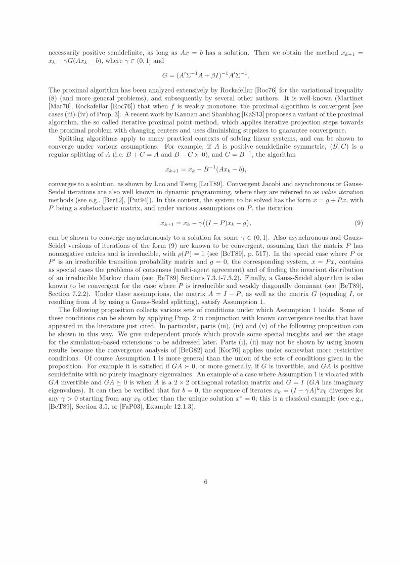
The proximal algorithm has been analyzed extensively by Rockafellar [Roc76] for the variational inequality(8) (and more general problems), and subsequently by several other authors. It is well-known (Martinet[Mar70], Rockafellar [Roc76]) that when f is weakly monotone, the proximal algorithm is convergent [seecases (iii)-(iv) of Prop. 3]. A recent work by Kannan and Shanbhag [KaS13] proposes a variant of the proximalalgorithm, the so called iterative proximal point method, which applies iterative projection steps towardsthe proximal problem with changing centers and uses diminishing stepsizes to guarantee convergence.

Splitting algorithms apply to many practical contexts of solving linear systems, and can be shown toconverge under various assumptions. For example, if A is positive semidefinite symmetric, (B,C) is aregular splitting of A (i.e. B + C = A and B − C ≻ 0), and G = B−1, the algorithm

xk+1 = xk −B−1(Axk − b),

converges to a solution, as shown by Luo and Tseng [LuT89]. Convergent Jacobi and asynchronous or Gauss-Seidel iterations are also well known in dynamic programming, where they are referred to as value iterationmethods (see e.g., [Ber12], [Put94]). In this context, the system to be solved has the form x = g +Px, withP being a substochastic matrix, and under various assumptions on P , the iteration

xk+1 = xk − γ(

(I − P )xk − g)

, (9)

can be shown to converge asynchronously to a solution for some γ ∈ (0, 1]. Also asynchronous and Gauss-Seidel versions of iterations of the form (9) are known to be convergent, assuming that the matrix P hasnonnegative entries and is irreducible, with ρ(P ) = 1 (see [BeT89], p. 517). In the special case where P orP ′ is an irreducible transition probability matrix and g = 0, the corresponding system, x = Px, containsas special cases the problems of consensus (multi-agent agreement) and of finding the invariant distributionof an irreducible Markov chain (see [BeT89] Sections 7.3.1-7.3.2). Finally, a Gauss-Seidel algorithm is alsoknown to be convergent for the case where P is irreducible and weakly diagonally dominant (see [BeT89],Section 7.2.2). Under these assumptions, the matrix A = I − P , as well as the matrix G (equaling I, orresulting from A by using a Gauss-Seidel splitting), satisfy Assumption 1.

The following proposition collects various sets of conditions under which Assumption 1 holds. Some ofthese conditions can be shown by applying Prop. 2 in conjunction with known convergence results that haveappeared in the literature just cited. In particular, parts (iii), (iv) and (v) of the following proposition canbe shown in this way. We give independent proofs which provide some special insights and set the stagefor the simulation-based extensions to be addressed later. Parts (i), (ii) may not be shown by using knownresults because the convergence analysis of [BeG82] and [Kor76] applies under somewhat more restrictiveconditions. Of course Assumption 1 is more general than the union of the sets of conditions given in theproposition. For example it is satisfied if GA ≻ 0, or more generally, if G is invertible, and GA is positivesemidefinite with no purely imaginary eigenvalues. An example of a case where Assumption 1 is violated withGA invertible and GA � 0 is when A is a 2 × 2 orthogonal rotation matrix and G = I (GA has imaginaryeigenvalues). It can then be verified that for b = 0, the sequence of iterates xk = (I − γA)kx0 diverges forany γ > 0 starting from any x0 other than the unique solution x∗ = 0; this is a classical example (see e.g.,[BeT89], Section 3.5, or [FaP03], Example 12.1.3).

6

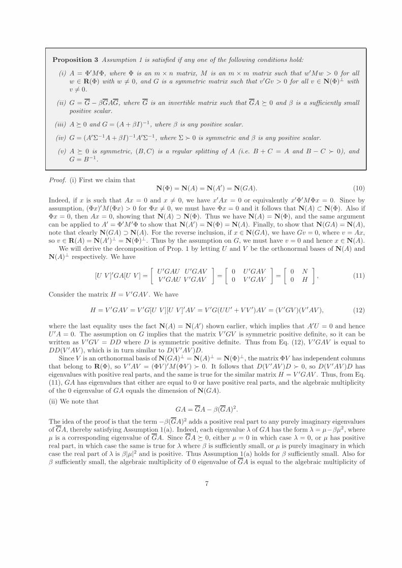
Proposition 3 Assumption 1 is satisfied if any one of the following conditions hold:

(i) A = Φ′MΦ, where Φ is an m × n matrix, M is an m × m matrix such that w′Mw > 0 for allw ∈ R(Φ) with w 6= 0, and G is a symmetric matrix such that v′Gv > 0 for all v ∈ N(Φ)⊥ withv 6= 0.

(ii) G = G − βGAG, where G is an invertible matrix such that GA � 0 and β is a sufficiently smallpositive scalar.

(iii) A � 0 and G = (A+ βI)−1, where β is any positive scalar.

(iv) G = (A′Σ−1A+ βI)−1A′Σ−1, where Σ ≻ 0 is symmetric and β is any positive scalar.

(v) A � 0 is symmetric, (B,C) is a regular splitting of A (i.e. B + C = A and B − C ≻ 0), andG = B−1.

Proof. (i) First we claim thatN(Φ) = N(A) = N(A′) = N(GA). (10)

Indeed, if x is such that Ax = 0 and x 6= 0, we have x′Ax = 0 or equivalently x′Φ′MΦx = 0. Since byassumption, (Φx)′M(Φx) > 0 for Φx 6= 0, we must have Φx = 0 and it follows that N(A) ⊂ N(Φ). Also ifΦx = 0, then Ax = 0, showing that N(A) ⊃ N(Φ). Thus we have N(A) = N(Φ), and the same argumentcan be applied to A′ = Φ′M ′Φ to show that N(A′) = N(Φ) = N(A). Finally, to show that N(GA) = N(A),note that clearly N(GA) ⊃ N(A). For the reverse inclusion, if x ∈ N(GA), we have Gv = 0, where v = Ax,so v ∈ R(A) = N(A′)⊥ = N(Φ)⊥. Thus by the assumption on G, we must have v = 0 and hence x ∈ N(A).

We will derive the decomposition of Prop. 1 by letting U and V be the orthonormal bases of N(A) andN(A)⊥ respectively. We have

[U V ]′GA[U V ] =

[

U ′GAU U ′GAVV ′GAU V ′GAV

]

=

[

0 U ′GAV0 V ′GAV

]

=

[

0 N0 H

]

, (11)

Consider the matrix H = V ′GAV . We have

H = V ′GAV = V ′G[U V ][U V ]′AV = V ′G(UU ′ + V V ′)AV = (V ′GV )(V ′AV ), (12)

where the last equality uses the fact N(A) = N(A′) shown earlier, which implies that A′U = 0 and henceU ′A = 0. The assumption on G implies that the matrix V ′GV is symmetric positive definite, so it can bewritten as V ′GV = DD where D is symmetric positive definite. Thus from Eq. (12), V ′GAV is equal toDD(V ′AV ), which is in turn similar to D(V ′AV )D.

Since V is an orthonormal basis ofN(GA)⊥ = N(A)⊥ = N(Φ)⊥, the matrix ΦV has independent columnsthat belong to R(Φ), so V ′AV = (ΦV )′M(ΦV ) ≻ 0. It follows that D(V ′AV )D ≻ 0, so D(V ′AV )D haseigenvalues with positive real parts, and the same is true for the similar matrix H = V ′GAV . Thus, from Eq.(11), GA has eigenvalues that either are equal to 0 or have positive real parts, and the algebraic multiplicityof the 0 eigenvalue of GA equals the dimension of N(GA).

(ii) We note thatGA = GA− β(GA)2.

The idea of the proof is that the term −β(GA)2 adds a positive real part to any purely imaginary eigenvaluesof GA, thereby satisfying Assumption 1(a). Indeed, each eigenvalue λ of GA has the form λ = µ−βµ2, whereµ is a corresponding eigenvalue of GA. Since GA � 0, either µ = 0 in which case λ = 0, or µ has positivereal part, in which case the same is true for λ where β is sufficiently small, or µ is purely imaginary in whichcase the real part of λ is β|µ|2 and is positive. Thus Assumption 1(a) holds for β sufficiently small. Also forβ sufficiently small, the algebraic multiplicity of 0 eigenvalue of GA is equal to the algebraic multiplicity of

7

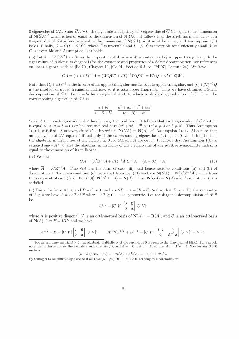
0 eigenvalue of GA. Since GA � 0, the algebraic multiplicity of 0 eigenvalue of GA is equal to the dimensionof N(GA),2 which is less or equal to the dimension of N(GA). It follows that the algebraic multiplicity of a0 eigenvalue of GA is less or equal to the dimension of N(GA), so it must be equal, and Assumption 1(b)holds. Finally, G = G(I − βAG), where G is invertible and I − βAG is invertible for sufficiently small β, soG is invertible and Assumption 1(c) holds.

(iii) Let A =WQW ′ be a Schur decomposition of A, where W is unitary and Q is upper triangular with theeigenvalues of A along its diagonal (for the existence and properties of a Schur decomposition, see referenceson linear algebra, such as [Bel70], Chapter 11, [Gol91], Section 6.3, or [TrB97], Lecture 24). We have

GA = (A+ βI)−1A = (WQW ′ + βI)−1WQW ′ =W (Q+ βI)−1QW ′.

Note that (Q+βI)−1 is the inverse of an upper triangular matrix so it is upper triangular, and (Q+βI)−1Qis the product of upper triangular matrices, so it is also upper triangular. Thus we have obtained a Schurdecomposition of GA. Let a + bi be an eigenvalue of A, which is also a diagonal entry of Q. Then thecorresponding eigenvalue of GA is

a+ bi

a+ β + bi=a2 + aβ + b2 + βbi

(a+ β)2 + b2.

Since A � 0, each eigenvalue of A has nonnegative real part. It follows that each eigenvalue of GA eitheris equal to 0 (a = b = 0) or has positive real part (a2 + aβ + b2 > 0 if a 6= 0 or b 6= 0). Thus Assumption1(a) is satisfied. Moreover, since G is invertible, N(GA) = N(A) [cf. Assumption 1(c)]. Also note thatan eigenvalue of GA equals 0 if and only if the corresponding eigenvalue of A equals 0, which implies thatthe algebraic multiplicities of the eigenvalue 0 for GA and A are equal. It follows that Assumption 1(b) issatisfied since A � 0, and the algebraic multiplicity of the 0 eigenvalue of any positive semidefinite matrix isequal to the dimension of its nullspace.

(iv) We haveGA = (A′Σ−1A+ βI)−1A′Σ−1A = (A+ βI)−1A, (13)

where A = A′Σ−1A. Thus GA has the form of case (iii), and hence satisfies conditions (a) and (b) ofAssumption 1. To prove condition (c), note that from Eq. (13) we have N(GA) = N(A′Σ−1A), while fromthe argument of case (i) [cf. Eq. (10)], N(A′Σ−1A) = N(A). Thus, N(GA) = N(A) and Assumption 1(c) issatisfied.

(v) Using the facts A � 0 and B −C ≻ 0, we have 2B = A+ (B −C) ≻ 0 so that B ≻ 0. By the symmetryof A � 0 we have A = A1/2A1/2 where A1/2 � 0 is also symmetric. Let the diagonal decomposition of A1/2

be

A1/2 = [U V ]

[

0 00 Λ

]

[U V ]′

where Λ is positive diagonal, V is an orthonormal basis of N(A)⊥ = R(A), and U is an orthonormal basisof N(A). Let E = UU ′ and we have

A1/2 + E = [U V ]

[

I 00 Λ

]

[U V ]′, A1/2(A1/2 + E)−1 = [U V ]

[

0 · I 00 Λ−1Λ

]

[U V ]′ = V V ′.

2For an arbitrary matrix A � 0, the algebraic multiplicity of the eigenvalue 0 is equal to the dimension of N(A). For a proof,note that if this is not so, there exists v such that Av 6= 0 and A2v = 0. Let u = Av so that Au = A2v = 0. Now for any β > 0we have

(u− βv)′A(u− βv) = −βu′Av + β2v′Av = −βu′u+ β2v′u.

By taking β to be sufficiently close to 0 we have (u− βv)′A(u− βv) < 0, arriving at a contradiction.

8

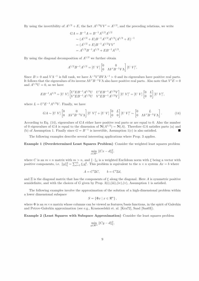
By using the invertibility of A1/2 + E, the fact A1/2V V ′ = A1/2, and the preceding relations, we write

GA = B−1A = B−1A1/2A1/2

∼ (A1/2 + E)B−1A1/2A1/2(A1/2 + E)−1

= (A1/2 + E)B−1A1/2V V ′

= A1/2B−1A1/2 + EB−1A1/2.

By using the diagonal decomposition of A1/2 we further obtain

A1/2B−1A1/2 = [U V ]

[

0 00 ΛV ′B−1V Λ

]

[U V ]′,

Since B ≻ 0 and V Λ−1 is full rank, we have Λ−1V ′BV Λ−1 ≻ 0 and its eigenvalues have positive real parts.It follows that the eigenvalues of its inverse ΛV ′B−1V Λ also have positive real parts. Also note that V ′E = 0and A1/2U = 0, so we have

EB−1A1/2 = [U V ]

[

U ′EB−1A1/2U U ′EB−1A1/2VV ′EB−1A1/2U V ′EB−1A1/2V

]

[U V ]′ = [U V ]

[

0 L0 0

]

[U V ]′,

where L = U ′E−1A1/2V . Finally, we have

GA ∼ [U V ]

[

0 00 ΛV ′B−1V Λ

]

[U V ]′ + [U V ]

[

0 L0 0

]

[U V ]′ ∼[

0 L0 ΛV ′B−1V Λ

]

. (14)

According to Eq. (14), eigenvalues of GA either have positive real parts or are equal to 0. Also the numberof 0 eigenvalues of GA is equal to the dimension of N(A1/2) = N(A). Therefore GA satisfies parts (a) and(b) of Assumption 1. Finally since G = B−1 is invertible, Assumption 1(c) is also satisfied. �

The following examples describe several interesting applications where Prop. 3 applies.

Example 1 (Overdetermined Least Squares Problem) Consider the weighted least squares problem

minx∈ℜn

‖Cx− d‖2ξ,

where C is an m×n matrix with m > n, and ‖ · ‖ξ is a weighted Euclidean norm with ξ being a vector withpositive components, i.e. ‖y‖2ξ =

∑mi=1 ξiy

2i . This problem is equivalent to the n× n system Ax = b where

A = C′ΞC, b = C′Ξd,

and Ξ is the diagonal matrix that has the components of ξ along the diagonal. Here A is symmetric positivesemidefinite, and with the choices of G given by Prop. 3(i),(iii),(iv),(v), Assumption 1 is satisfied.

The following examples involve the approximation of the solution of a high-dimensional problem withina lower dimensional subspace

S = {Φx | x ∈ ℜn} ,where Φ is an m×n matrix whose columns can be viewed as features/basis functions, in the spirit of Galerkinand Petrov-Galerkin approximation (see e.g., Krasnoselskii et. al. [Kra72], Saad [Saa03]).

Example 2 (Least Squares with Subspace Approximation) Consider the least squares problem

miny∈ℜm

‖Cy − d‖2ξ,

9

where C and d are given s ×m matrix and vector in ℜs, respectively, and ‖ · ‖ξ is the weighted Euclideannorm of Example 1. By approximating y within the subspace S = {Φx | x ∈ ℜn} , we obtain the least squaresproblem

minx∈ℜn

‖CΦx− d‖2ξ.

This is equivalent to the n× n linear system Ax = b where

A = Φ′C′ΞCΦ, b = Φ′C′Ξd.

Similar to Example 1, A is symmetric positive semidefinite. With the choices ofG given by Prop. 3(i),(iii),(iv),(v), Assumption 1 is satisfied. Simulation-based noniterative methods using the formulation of this examplewere proposed in Bertsekas and Yu [BeY09], while iterative methods were proposed in Wang et al. [WPB09]and tested on large-scale inverse problems in Polydorides et al. [PWB10]. The use of simulation may bedesirable in cases where either s or m, or both, are much larger than n. In such cases the explicit calculationof A may be difficult.

The next two examples involve a nonsymmetric matrix A. They arise in the important context of policyiteration in approximate dynamic programming (ADP for short); see e.g., the books [BeT89] and [SuB98],and the recent survey [Ber11].

Example 3 (Projected Equations with Subspace Approximation) Consider a projected version ofan m×m fixed point equation y = Py + g given by

Φx = Πξ(PΦx+ g),

where Πξ denotes orthogonal projection onto the subspace S with respect to the weighted Euclidean ‖ · ‖ξof Examples 1 and 2 (in ADP, P is a substochastic matrix and g is the one-stage cost vector). By writingthe orthogonality condition for the projection, it can be shown that this equation is equivalent to the n× nsystem Ax = b where

A = Φ′Ξ(I − P )Φ, b = Φ′Ξg.

Various conditions guaranteeing that A � 0 or A ≻ 0 are given in [BeY09] and [Ber11], and they involvecontraction properties of the mappings ΠξP and P . Examples are standard Markov and semi-Markovdecision problems, where y′Ξ(I − P )y > 0 for all y ∈ R(Φ) with y 6= 0 and an appropriate choice of Ξ, andA � 0, so with the choices of G given by Prop. 3(i),(iii),(iv), Assumption 1 is satisfied.

Example 4 (Oblique Projected Equations and Aggregation) The preceding example of projected e-quations Φx = Πξ(g + Px) can be generalized to the case where Πξ is an oblique projection, i.e., its rangeis S = {Φx | x ∈ ℜn} and is such that Π2

ξ = Πξ. Let Ψ be an m × n matrix such that R(Ψ) does notcontain any vector orthogonal to R(Φ), and let Πξ be the weighted oblique projection such that Πξy ∈ Sand (y −Πξy)

′ΞΨ = 0 for all y ∈ ℜm. The optimality condition associated with the projected equation is

Ψ′ΞΦx = Ψ′Ξ(g + PΦx),

which is equivalent to the n× n system Ax = b where

A = Ψ′Ξ(I − P )Φ, b = Ψ′Ξg.

We don’t necessarily have A ≻ 0 or A � 0 even if P is a substochastic matrix. With the choice of G givenby Prop. 3(iv), Assumption 1 is satisfied.

One special case where oblique projections arise in ADP is an aggregation equation of the form

Φx = ΦD(g + αPΦx),

where α ∈ (0, 1], D is an n ×m matrix, and the n-dimensional rows of Φ and the m-dimensional rows ofD are probability distributions (see [Ber12]). Assume that for a collection of n mutually disjoint subsets of

10

the index set {1, . . . ,m}, I1, . . . , Im, we have dji > 0 only if i ∈ Ij and φij = 1 if i ∈ Ij . Then it can beverified that DΦ = I hence (ΦD)2 = ΦD, so ΦD is an oblique projection matrix. The aggregation equationis equivalent to the n× n system Ax = b where

A = I − αDPΦ, b = Dg.

In standard discounted problems, DPΦ is a stochastic matrix and α < 1. Then iteration (9) where G = Iand γ ∈ (0, 1] is convergent. For additional choices of G such that Assumption 1 is satisfied, we refer to thediscussion following Eq. (9).

2.3 Simulation-Based Methods

We will now consider a simulation-based version of the deterministic method (3). It has the form

xk+1 = xk − γGk(Akxk − bk), (15)

where Ak, bk, and Gk, are estimates of A, b, and G, respectively. Throughout our analysis, we assume thefollowing.

Assumption 2 The sequence {Ak, bk, Gk} is generated by a stochastic process such that

Aka.s.−→ A, bk

a.s.−→ b, Gka.s.−→ G.

Assumption 2 is a general assumption that applies to practical situations involving a stochastic simula-tor/sampler. In many of these applications, the simulation process generates an infinite sequence of randomvariables

{

(Wt, vt) | t = 1, 2, . . .}

,

where Wt is an n× n matrix and vt is a vector in ℜn, and estimates A and b with Ak and bk given by

Ak =1

k

k∑

t=1

Wt, bk =1

k

k∑

t=1

vt. (16)

For instance, the sample sequence may consist of independent samples from a certain distribution (e.g.,Drineas et al. [DMM06]) or from a sequence of importance sampling distributions. Also, the sample sequencecan be generated through state transitions of an irreducible Markov chain, as for example in temporaldifference methods in the context of ADP (e.g., [BrB96], [Boy02], [NeB03], and [Ber10]), or for generalprojected equations (e.g., [BeY09], [Ber11]).

Stochastic algorithms that use Monte Carlo estimates of the form (16) have a long history in stochasticprogramming and applies to a wide range of problems under various names (for recent theoretical develop-ments, see Shapiro [Sha03], and for applications in ADP, see [BeT96]). The proposed method in the currentwork uses increasingly accurate approximations, obtained from some sampling process, to replace unknownquantities in deterministic algorithms that are known to be convergent. A related method, known as thesample average approximation method (SAA), approximates the original problem by using a fixed numberof samples obtained from pre-sampling (e.g., see Shapiro et al. [SDR09] for a book account, and relatedpapers such as Kleywegt et al. [KSH02], and Nemirovskii et al. [NJL09]). A variant of SAA is the so-calledretrospective approximation method (RA), which solves a sequence of SAA problems by using an increasingnumber of samples for each problem (see e.g., Pasupathy [Pas10]). Our method differs from RA in that ouralgorithm is an iterative one-time scale method that uses increasingly accurate approximations in the iter-ation, instead of solving a sequence of increasingly accurate approximate systems. Throughout this paper,we avoid defining explicitly {Ak, bk, Gk} as sample averages, so our analysis applies to a more general classof stochastic methods.

11

Another related major class of methods, known as the stochastic approximation method (SA), uses asingle sample per iteration and a decreasing sequence of stepsizes {γk} to ensure convergence (see e.g.,[BMP90], [Bor08], [KuY03], and [Mey07] for textbook discussions, and see Nemirovski et al. [NJLS09] for arecent comparison between SA and SAA). Our methodology differs in fundamental ways from SA. While theSA method relies on decreasing stepsizes to control the convergence process, our methodology is based onMonte-Carlo estimates uses a constant stepsize, which implies a constant modulus of contraction as well asmultiplicative (rather than additive) noise. This both enhances its performance and complicates its analysiswhen A is singular, as it gives rise to large stochastic perturbations that must be effectively controlled toguarantee convergence.

We will first illustrate some possibilities for obtaining {Ak, bk, Gk} by simulation, based on the appli-cations of Examples 1-4. As noted earlier, the use of simulation in these applications aims to deal withlarge-scale linear algebra operations, which would be very time consuming or impossible if done exactly. Inthe first application we aim to solve approximately an overdetermined system by randomly selecting a subsetof the constraints; see [DMM06], [DMMS11].

Example 5 (Continued from Example 1) Consider the least squares problem of Example 1, which isequivalent to the n× n system Ax = b where

A = C′ΞC, b = C′Ξd.

We generate a sequence of i.i.d. indices {i1, . . . , ik} according to a distribution ζ, and estimate A and b usingEq. (16), where

Wt =ξitζitcitc

′it , vt =

ξitζitcitdit ,

c′i is the ith row of C, and ξi is the ith diagonal component of Ξ.

Example 6 (Continued from Example 2) Consider the least squares problem of Example 2, which isequivalent to the n× n system Ax = b where

A = Φ′C′ΞCΦ, b = Φ′C′Ξd.

We generate i.i.d. indices {i1, . . . , ik} according to a distribution ζ, and then generate two sequences of inde-pendent state transitions {(i1, j1), . . . (ik, jk)} and {(i1, ℓ1), . . . (ik, ℓk)} according to transition probabilitiespij (i.e., given ik, generate (ik, jk) with probability pikjk). We may then estimate A and b using Eq. (16),where

Wt =ξitcitjtcitℓtζitpitjtpitℓt

φjtφ′ℓt , vt =

ξitcitjtζitpitjt

φitdjt ,

φ′i is the ith row of Φ, and cij is the (i, j)th component of C.

Example 7 (Continued from Example 3) Consider the projected equation of Example 3, which is e-quivalent to the n× n system Ax = b where

A = Φ′Ξ(I − P )Φ, b = Φ′Ξg.

One approach is to generate a sequence of i.i.d. indices {i1, . . . , ik} according to distribution ζ, and generatea sequence of state transitions {(i1, j1), . . . (ik, jk)} according to transition probabilities θij . We may thenestimate A and b using Eq. (16), where

Wt =ξitζitφit

(

φit −pitjtθitjt

φjt

)′, vt =

ξitζitφitgit ,

pij denotes the (i, j)th component of the matrix P .In an alternative approach, which applies to cost evaluation of discounted ADP problems, the matrix P

is the transition probability matrix of an irreducible Markov chain. We use the Markov chain instead of i.i.d.

12

indices for sampling. In particular, we take ξ to be the invariant distribution of the Markov chain. We thengenerate a sequence {i1, . . . , ik} according to this Markov chain, and estimate A and b using Eq. (16), where

Wt = φit(φit − φit+1)′, vt = φitgit .

It can be verified that Ak =1

k

k∑

t=1

Wta.s.−→ A and bk =

1

k

k∑

t=1

vta.s.−→ b by the strong law of large numbers for

irreducible Markov chains.

Example 8 (Continued from Example 4) Consider the projected equation using oblique projection ofExample 4, which is equivalent to the n× n system Ax = b where

A = Ψ′Ξ(I − P )Φ, b = Ψ′Ξg.

We may generate a sequence of i.i.d. indices {i1, . . . , ik} according to distribution ζ, generate a sequence ofstate transitions {(i1, j1), . . . , (ik, jk)} according to transition probabilities θij , and estimate A and b usingEq. (16), where

Wt =ξitζitψit

(

φit −pitjtθitjt

φjt

)′, vt =

ξitζitψitgit ,

ψ′i denotes the ith row of the matrix Ψ.In the special case of the aggregation equation Φx = ΦD(g + αPΦx) where P is a transition probability

matrix, this is equivalent to Ax = b where

A = I − αDPΦ, b = Dg.

We may generate i.i.d. indices {i1, . . . , ik} according to a distribution ζ, generate a sequence of state transi-tions {(i1, j1), . . . , (ik, jk)} according to P , and estimate A and b using Eq. (16), where

Wt = I − α

ζitditφ

′jt , vt =

gitζitdit ,

and di is the ith column of D.

Note that the simulation formulas used in Examples 5-8 satisfy Assumption 2, and only involve low-dimensional linear algebra computations. In Example 5, this is a consequence of the low dimension n of thesolution space of the overdetermined system. In Examples 6-8, this is a consequence of the low dimension nof the approximation subspace defined by the basis matrix Φ.

Even if Assumptions 1, 2 are both satisfied, iteration (15) does not necessarily converge to any solution.To understand the reason, let us consider the decomposition of the iteration into the components Uykand V zk within N(A) and N(A)⊥, respectively (cf. Prop. 1). Then contrary to the case where there is nosimulation error [cf. Eq. (4)], zk is no longer decoupled from yk, and may become contaminated by additionalsimulation noise through the yk iterates, which are not governed by a contractive process. The decomposediteration takes the form

yk+1 = yk − γ Nzk + ζk(yk, zk), zk+1 = zk − γHzk + ξk(yk, zk), (17)

where ζk(yk, zk) and ξk(yk, zk) are simulation-induced errors that are functions of yk and zk [compare withEq. (4)]. Generally, these errors converge to 0 if {yk} and {zk} are bounded, in which case zk converges to0 (since I − γH is a contraction for appropriate γ by Prop. 1). However, yk need not stay bounded, and asa result the sequence {xk} generally does not converge. On the other hand, the residual sequence {Axk − b}is better behaved than {xk}. An important fact in this regard is Axk − b = A(xk − x∗) (where x∗ is anysolution of Ax = b), so it depends only on the component of xk − x∗ that belongs to N(A)⊥.

13

To address the divergence of the iteration, a class of modification/stabilization schemes for iteration(15) has been proposed in the related work [WaB11], which aims to attenuate the effect of accumulatingsimulation errors. One such modification is

xk+1 = (1− δk)xk − γGk(Akxk − bk), (18)

whereby the eigenvalues of the iteration are shifted by −δk, and δk ↓ 0 at a rate that is slower than the rateof convergence of (GkAk−GA, bk−b). It was shown that in this case, {xk} converges to a specific solution ofAx = b with probability 1. This stabilization approach can be applied to an arbitrary stochastic iteration ofthe form (15), provided that the corresponding deterministic iteration is convergent. Another modificationis the selective eigenvalue shifting scheme given by

xk+1 =(

1− δk(I −Πk))

xk − γGk(Akxk − bk), (19)

where Πk converges to the orthogonal projection matrix onto N(A)⊥, and I−Πk converges to the projectionmatrix onto N(A). This scheme requires an estimated projection matrix, and selectively shifts only thoseeigenvalues corresponding to N(A). It was proved that under reasonable assumptions, iteration (19) con-verges to the solution of Ax = b with minimal Euclidean norm (the Moore-Penrose pseudoinverse solution).We will return to the problem of estimating Πk in Section 6. A related work by Koshal et al. [KNS12]considers an iterative Tikhonov regularization method for stochastic variational inequalities, which uses adiminishing regularization term that has an effect similar to our stabilization term. This method differsfrom the method of Eqs. (18)-(19) in that it requires a diminishing stepsize γk, and it does not involve themultiplicative noise (i.e., Akxk − bk).

In the following sections, we will focus on the convergence of two algorithms of the form (15), for whichit is unnecessary to use stabilization:

(a) When the nullspace of the iteration “remains stable,” i.e.,

N(GkAk) = N(Ak) = N(A) = N(GA).

In this case, zk does not depend on yk and converges to 0, and the same is true for the residualAxk − b = AV zk [cf. Eqs. (4) and (5)]. Moreover, under some additional special conditions, we canshow that yk also converges. This analysis will be given in Section 3.

(b) When a proximal iteration involving quadratic regularization is applied to the system A′Σ−1Ax =A′Σ−1b. This iteration is given by

xk+1 = xk −(

A′kΣ

−1Ak + βI)−1

A′kΣ

−1(Akxk − bk),

where β is a positive scalar. Here the special structure of the matrices Gk = (A′kΣ

−1Ak+βI)−1A′

kΣ−1

is such that I − GkAk is contractive for all k. Under an additional assumption on the convergencerate of {Ak, bk, Gk}, this structure forces the residual to converge to 0. This analysis will be given inSection 4.

While in both of the above cases the sequence of residuals {Axk − b} is convergent to 0 with probability 1,the sequence of iterates {xk} may be unbounded. In order to extract from {xk} a convergent sequence, wewill propose in Section 6 two approaches for estimating the matrix of projection onto N(A)⊥, and we willapply them to the preceding algorithms.

2.4 Choice of the Stepsize γ

An important issue is how to select an appropriate stepsize γ in the simulation-based iterations. In theory,the stepsize γ needs to be sufficiently small, proportional to the smallest positive part of eigenvalues of GA(see Prop. 2). In practice and in the presence of simulation noise, determining γ can be challenging, given

14

that A and b are largely unknown. This is particularly so for singular or nearly singular problems, since thenthe close-to-zero eigenvalues of GA are hard to estimate precisely. In this section we address this issue forseveral different cases.

In the cases of a proximal point iteration or a splitting iteration [e.g., cases (iii)-(v) in Prop. 3], we maysimply take γ = 1, as noted in Section 2.2. For other cases, one possibility is to estimate a value of γ tosatisfy γ ∈ (0, γ), where γ is given by Eq. (6), based on the sampling process, while another is to use adiminishing stepsize, as we describe in what follows.

To estimate an appropriate value of γ, we may update an upper bound of stepsize according to

γk+1 =

{

γk if ρ(I − γkGkAk) ≤ 1 + δk,ηkγk if ρ(I − γkGkAk) > 1 + δk,

(20)

where {δk} is a slowly diminishing positive sequence and {ηk} is a sequence in (0, 1), and choose the stepsizeaccording to

γk ∈ (0, γk).

Under suitable conditions, which guarantee that δk eventually becomes an upper bound of the maximumperturbation in eigenvalues of GkAk, we can verify that γk converges to some point within the interval (0, γ],as shown in the following proposition.

Proposition 4 Let Assumptions 1-2 hold, let {ηk} be a sequence of positive scalars such that∏∞

k=0 ηk =

0, and let {δk} be a sequence of positive scalars such that δk ↓ 0 and ǫk/δka.s.−→ 0, where

ǫk = maxi=1,...,n

∣

∣λi(GkAk)− λi(GA)∣

∣,

with λi(M) denoting the ith eigenvalue of a matrix M . Then, with probability 1, the sequence {γk}generated by iteration (20) converges to some value in (0, γ] within a finite number of iterations.

Proof. By its definition, {γk} either converges to 0 or stays constant at some positive value for all ksufficiently large. Assume to arrive at a contradiction that γk eventually stays constant at some γ > γ, suchthat ρ(I − γGA) > 1 (cf. the analysis of Prop. 2). Note that for any γ, k > 0, we have

|ρ(I − γGkAk)− ρ(I − γGA)| ≤ γ maxi=1,...,n

∣

∣λi(GkAk)− λi(GA)∣

∣ = γǫk.

From the preceding relation, we have

ρ(I − γkGkAk) = ρ(I − γGkAk) ≥ ρ(I − γGA)− γǫk > 1 + δk,

for sufficiently large k with probability 1, where we used the facts δk ↓ 0, GkAka.s.−→ GA (cf. Assumption

2), so that ǫka.s.−→ 0 (see e.g., the book on matrix perturbation theory by Stewart and Sun [StS90]). Thus

according to iteration (20), γk needs to be decreased again, yielding a contradiction. It follows that γkeventually enters the interval (0, γ] such that ρ(I − γGA) ≤ 1 for all γ ∈ (0, γ], with probability 1.

Once γk enters the interval (0, γ], we have

ρ(I − γkGkAk) ≤ ρ(I − γkGA) + γkǫk ≤ 1 + δk,

for all k sufficiently large with probability 1, where we used the fact ǫk/δka.s.−→ 0 and the boundedness of

{γk}. This together with Eq. (20) imply that γk eventually stays constant at a value within (0, γ]. �

In the preceding approach, the error tolerance sequence δk needs to decrease more slowly than ǫk, thesimulation errors in eigenvalues. Based on matrix perturbation theory, as GkAk

a.s.−→ GA, we have ǫk ≤O(‖GkAk − GA‖p), where p = 1 if GA is diagonalizable and p = 1/n otherwise (see [StS90] p. 192 and p.

15

168). This allows us to choose δk in accordance with the convergence rate of simulation error. Moreover, thesequence ηk can be selected as ηk = η ∈ (0, 1), or ηk = 1 − 1/k, etc. Finally, accordingly to the precedinganalysis, the stepsize γk can be selected to converge finitely to an appropriate stepsize value γ within (0, γ)for k sufficiently large with probability 1. Thus our convergence analysis for constant stepsizes applies.

The preceding estimation procedure requires some extra overhead to compute the spectral radius ρ(I −γkGkAk). A simpler alternative is to replace the constant stepsize γ with a diminishing stepsize γk ↓ 0. Aslong as

∑∞k=0 γk = ∞, our convergence analysis can be adapted to work with such stepsizes. This approach

avoids the estimation of γ, but it may be less desirable because it degrades the linear rate of convergence ofthe residuals, which is guaranteed if the stepsize is not diminished to 0.

The details of the extensions of our convergence analysis to the stepsize schemes described above arerelatively simple and will not be given. To sum up, if γ cannot be properly chosen based on generalproperties of the corresponding deterministic algorithm, it can be estimated based on the sampling processto ensure convergence, or simply taken to be diminishing. In what follows, we will assume that γ is chosento be a constant.

3 Nullspace-Consistent Simulation-Based Iterations

In this section, we consider a special case of the iterative method (15) under an assumption that parallelsAssumption 1. It requires that the rank and the nullspace of the matrix GkAk do not change as we pass tothe limit. As a result the nullspace decomposition that is associated with GA (cf. Prop. 1) does not changeas the iterations proceed.

Assumption 3

(a) Each eigenvalue of GA either has a positive real part or is equal to 0.

(b) The dimension of N(GA) is equal to the algebraic multiplicity of the eigenvalue 0 of GA.

(c) With probability 1, there exists an index k such that

N(A) = N(Ak) = N(GkAk) = N(GA), ∀ k ≥ k. (21)

If the stochastic iteration (15) satisfies Assumption 3, we say that it is nullspace-consistent. SinceAssumption 3 implies Assumption 1, the corresponding deterministic iteration xk+1 = xk − γG(Axk − b) isconvergent. The key part of the assumption, which is responsible for its special character in a stochasticsetting, is part (c).

Let us describe an important special case where Assumption 3 holds. Suppose that A and Ak are of theform

A = Φ′MΦ, Ak = Φ′MkΦ,

where Φ is an m× n matrix, M is an m×m matrix with y′My > 0 for all y ∈ R(Φ) with y 6= 0, and Mk isa sequence of matrices such that Mk → M . Examples 2, 3, 6, and 7 satisfy this condition. Assuming thatG is invertible, we can verify that Assumption 3(c) holds. Moreover if G is positive definite symmetric, byusing Prop. 3(i) we obtain that Assumption 3(a),(b) also hold. We will return to this special case in Section3.2.

3.1 Convergence of Residuals

We will now show that for nullspace-consistent iterations, the residual sequence {Axk − b} always convergesto 0, regardless of whether the iterate sequence {xk} diverges. The idea is that, under Assumption 3, thematrices U and V of the nullspace decomposition of I − γGA remain unchanged as we pass to the nullspace

16

decomposition of I − γGkAk. This induces a favorable structure of the zk-portion of the iteration, anddecouples it from yk [cf. Eq. (17)].

Proposition 5 (Convergence of Residual for Nullspace-Consistent Iteration) Let Assumptions2 and 3 hold. Then there exists a scalar γ > 0, such that for all γ ∈ (0, γ] and every initial iterate x0,the sequence {xk} generated by iteration (15) satisfies Axk − b → 0 and Akxk − bk → 0 with probability1.

Proof. Let x∗ be the solution of Ax = b with minimal Euclidean norm. Then iteration (15) can be writtenas

xk+1 − x∗ = (I − γGkAk)(xk − x∗) + γGk(bk −Akx∗). (22)

In view of nullspace-consistency, the nullspace decomposition of GA of Prop. 1 can also be applied fornullspace decomposition of I − γGkAk. Thus, with probability 1 and for sufficiently large k, we have

[U V ]′(I − γGkAk) [U V ] =

[

I −γU ′GkAkV0 I − γV ′GkAkV

]

,

where the zero block in the second row results from the assumption N(Ak) = N(A) [cf. Eq. (21)], so

V ′(I − γGkAk)U = V ′U − γV ′GkAkU = V ′U − 0 = 0.

Recalling the iteration decompositionxk = x∗ + Uyk + V zk,

we may rewrite iteration (22) as

[

yk+1

zk+1

]

=

[

I −γU ′GkAkV0 I − γV ′GkAkV

] [

ykzk

]

+

[

γU ′GkekγV ′Gkek

]

, (23)

where ek = bk − Akx∗. Note that the zk-portion of this iteration is independent of yk. Focusing on the

asymptotic behavior of iteration (23), we observe that:

(a) The matrix I − γV ′GkAkV converges almost surely to I − γV ′GAV = I − γH , which is contractivefor sufficiently small γ > 0 (cf. the proof of Prop. 2).

(b) γV ′Gkeka.s.−→ 0, because Gk

a.s.−→ G and eka.s.−→ 0.

Therefore the zk-portion of iteration (23) is strictly contractive for k sufficiently large with additive error

decreasing to 0, implying that zka.s.−→ 0. Finally, since Axk − b = AV zk, it follows that Axk − b

a.s.−→ 0.Moreover, we have

Akxk − bk = Ak(xk − x∗) + (Akx∗ − bk) = Ak(Uyk + V zk) + (Akx

∗ − bk) = AkV zk + (Akx∗ − bk)

a.s.−→ 0,

where the last equality uses the fact AkU = 0. Thus we also have Akxk − bka.s.−→ 0. �

The proof of the preceding proposition shows that for a given stepsize γ > 0, the residual of the nullspace-consistent stochastic iteration

xk+1 = xk − γGk(Akxk − bk)

converges to 0 if and only if the matrix I − γGA is a contraction in N(A)⊥. This is also the necessary andsufficient condition for the residual sequence generated by the deterministic iteration

xk+1 = xk − γG(Axk − b)

17

to converge to 0 (and also for {xk} to converge to some solution of Ax = b).Note that the sequence {xk} may diverge; see Example 12 in Section 5. To construct a convergent

sequence, we note that by Assumption 3, N(Ak) = N(A), so we can obtain the projection matrix from

ΠN(A)⊥ = A′k(AkA

′k)

†Ak,

where (AkA′k)

† is the Moore-Penrose pseudoinverse of AkA′k. Applying this projection to xk yields the vector

xk = ΠN(A)⊥xk = ΠN(A)⊥(x∗ + Uyk + V zk) = x∗ + V zk,

where x∗ is the minimum norm solution of Ax = b. Since zka.s.−→ 0, we have xk

a.s.−→ x∗.

3.2 Convergence of Iterates

We now turn to deriving conditions under which {xk} converges naturally. This requires that the first rowin Eq. (23) has the appropriate asymptotic behavior.

Proposition 6 (Convergence of Nullspace-Consistent Iteration) Let Assumptions 2 and 3 hold,and assume in addition that

R(GkAk) ⊂ N(A)⊥, Gkbk ∈ N(A)⊥, (24)

for k sufficiently large. Then there exists γ > 0 such that for all γ ∈ (0, γ] and all initial iterates x0, thesequence {xk} generated by iteration (15) converges to a solution of Ax = b with probability 1.

Proof. With the additional conditions (24), we have

γU ′GkAkV = 0, γU ′Gk(bk −Akx∗) = 0,

for all k sufficiently large, so that the first row of Eq. (23) becomes yk+1 = yk. Since Prop. 5 implies that

zka.s.−→ 0, it follows that xk converges with probability 1, and its limit is a solution of Ax = b. �

We now revisit the special case discussed following Assumption 3, and prove the convergence of {xk}.This case arises in the context of ADP (cf. Examples 2, 3, 6, 7), and the convergence of iteration (15)within that context has been discussed in [Ber11]. It involves the approximation of the solution of a high-dimensional equation within a lower-dimensional subspace spanned by a set of n basis functions that comprisethe columns of an m× n matrix Φ where m≫ n. This structure is captured by the following assumption.

Assumption 4

(a) The matrix Ak has the formAk = Φ′MkΦ,

where Φ is an m× n matrix, and Mk is an m×m matrix that converges to a matrix M such thaty′My > 0 for all y ∈ R(Φ) with y 6= 0.

(b) The vector bk has the formbk = Φ′dk, (25)

where dk is a vector in ℜm that converges to some vector d.

(c) The matrix Gk converges to a matrix G satisfying Assumption 1 together with A = Φ′MΦ, andsatisfies for all k

GkR(Φ′) ⊂ R(Φ′). (26)

18

We have the following proposition.

Proposition 7 Let Assumption 4 hold. Then the assumptions of Prop. 6 are satisfied, and there existsγ > 0 such that for all γ ∈ (0, γ] and all initial iterates x0, the sequence {xk} generated by iteration (15)converges to a solution of Ax = b with probability 1.

Proof. Assumption 4(c) implies Assumption 1, so parts (a) and (b) of Assumption 3 are satisfied. Accordingto the analysis of Prop. (3)(i), Assumption 4(a) implies that

N(Φ) = N(A) = N(A′) = N(Ak) = N(A′k) = N(GA) = N(GkAk). (27)

Thus, parts (a) and (c) of Assumption 4 imply Assumption 3, and together with Assumption 4(b), theyimply Assumption 2 as well.

From Eq. (27), we have

R(Φ′) = N(Φ)⊥ = N(A)⊥ = N(Ak)⊥ = N(A′

k)⊥ = R(Ak).

Hence using the assumption GkR(Φ′) ⊂ R(Φ′) and the form of bk given in Eq. (25), we have

R(GkAk) = GkR(Ak) = GkR(Φ′) ⊂ R(Φ′) = N(A)⊥,

andGkbk ∈ GkR(Φ′) ⊂ R(Φ′) = N(A)⊥.

Hence the conditions (24) are satisfied. �

We now give a few interesting choices of Gk such that Assumption 4 is satisfied and {xk} converges to asolution of Ax = b.

Proposition 8 Let Assumption 4(a),(b) hold, and let Gk have one of the following forms:

(i) Gk = I.

(ii) Gk = (Φ′ΞkΦ + βI)−1, where Ξk converges to a positive definite diagonal matrix and β is anypositive scalar.

(iii) Gk = (Ak + βI)−1, where β is any positive scalar.

(iv) Gk = (A′kΣ

−1Ak + βI)−1A′kΣ

−1, where Σ is any positive definite symmetric matrix.

Then Assumption 4(c) is satisfied. Moreover, there exists γ > 0 such that for all γ ∈ (0, γ] and allinitial iterates x0, the sequence {xk} generated by iteration (15) converges to a solution of Ax = b withprobability 1.

Proof. First note that the inverses in parts (ii)-(iv) exist [for case (iii), Gk is invertible for sufficiently largek, since from Assumption 4(a), x′(Ak + βI)x = x′Φ′MkΦx + β‖x‖2 > 0 for all x 6= 0]. We next verify thatGk converges to a limit G, which together A = Φ′MΦ satisfies Assumption 1. For cases (i)-(ii), Gk convergesto a symmetric positive definite matrix, so Assumption 1 holds; see Prop. 3(i) of [WaB11]. For cases (iii)and (iv), these two iterations are proximal algorithms so Assumption 1 holds; see Prop. 3 (iii)-(iv). We areleft to verify the condition GkR(Φ′) ⊂ R(Φ′) [cf. Eq. (26)].

In cases (i)-(iii), we can show that Gk always takes the form

Gk = (Φ′NkΦ+ βI)−1,

19

where Nk is an appropriate matrix and β is a positive scalar [to see this for case (i), we take Nk = 0 andβ = 1; for case (ii) we take Nk = Ξk; for case (iii), recall that Ak = Φ′MkΦ and let Nk =Mk]. Let v ∈ R(Φ′)and let h be given by h = Gkv. Since Gk is invertible, we have

v = G−1k h = (Φ′NkΦ + βI)h.

Since v ∈ R(Φ′), we must haveΦ′NkΦh+ βh ∈ R(Φ′).

Note that Φ′NkΦh ∈ R(Φ′), so we must have βh ∈ R(Φ′). Thus we have shown that h = Gkv ∈ R(Φ′) forany v ∈ R(Φ′), or equivalently,

(Φ′NkΦ+ βI)−1R(Φ′) ⊂ R(Φ′). (28)

In case (iv), we can write Gk in the form of

Gk = (Φ′NkΦ+ βI)−1A′kΣ

−1,

where Nk =M ′kΦΣ

−1Φ′Mk. For any v ∈ R(Φ′), we have

h = Gkv = (Φ′NkΦ+ βI)−1(A′kΣ

−1v).

Note that A′kΣ

−1v = Φ′M ′kΦΣ

−1v ∈ R(Φ′), so by applying Eq. (28) we obtain h ∈ R(Φ′). Thus our proofof GkR(Φ′) ⊂ R(Φ′) is complete for all cases (i)-(iv). �

4 Simulation-Based Proximal Iteration with Quadratic Regular-

ization

We now consider another special case of the simulation-based iteration

xk+1 = xk − γGk(Akxk − bk), (29)

where the residuals converge to 0 naturally. It may be viewed as a proximal iteration, applied to thereformulation of Ax = b as the least squares problem

minx∈ℜn

(Ax− b)′Σ−1(Ax − b),

or equivalently the optimality condition/linear system

A′Σ−1Ax = A′Σ−1b, (30)

where Σ is a symmetric positive definite matrix. Generally, proximal iterations are applicable to systemsinvolving a positive semidefinite matrix. By considering instead the system (30), we can bypass this require-ment, and apply a proximal algorithm to any linear system Ax = b that has a solution, without A beingnecessarily positive semidefinite, since the matrix A′Σ−1A is positive semidefinite for any A.

Consider the following special choice of the scaling matrix Gk and its limit G:

Gk = (A′kΣ

−1Ak + βI)−1A′kΣ

−1, G = (A′Σ−1A+ βI)−1A′Σ−1,

where β is a positive scalar. We use γ = 1 and write iteration (29) as

xk+1 = xk − (A′kΣ

−1Ak + βI)−1A′kΣ

−1(Akxk − bk), (31)

which is equivalent to the sequential minimization

xk+1 = argminx∈ℜn

{

1

2(Akx− bk)

′Σ−1(Akx− bk) +β

2‖x− xk‖2

}

20

that involves the regularization term (β/2)‖xk − x‖2; see case (iv) of Prop. 3.It can be shown that this iteration is always nonexpansive, i.e.

‖I −GkAk‖ ≤ 1, ∀ k,

due to the use of regularization. However, the convergence analysis is complicated when A is singular, inwhich case

limk→∞

ρ(I −GkAk) = ρ(I −GA) = 1.

Then the mappings from xk to xk+1 are not uniformly contractive, i.e., with a uniform modulus bounded bysome η ∈ (0, 1) for all sufficiently large k. Thus, to prove convergence of the residuals, we must show thatthe simulation error accumulates at a relatively slow rate in N(A). For this reason we need some assumptionregarding the rate of convergence of Ak, bk, and Gk like the following.

Assumption 5 The simulation error sequence,

Ek = (Ak −A, bk − b,Gk −G),

viewed as a (2n2 + n)-vector, satisfies

lim supk→∞

kp E{

‖Ek‖2p}

<∞,

for some p > 2.

Assumption 5 applies to most practical situations that involve Monte Carlo sampling, such as i.i.d. sam-pling, importance sampling, and Markov chain sampling (see the discussions in Section 2.3). Under naturalconditions (e.g., bounded support, subgaussian tail distribution, etc), these simulation methods satisfy As-sumption 5 through forms of the central limit theorem and some concentration inequality arguments.3 Adetailed analysis for various situations where Assumption 5 holds requires dealing with technicalities of the

3We will give a brief proof that Assumption 5 holds for the case where Xk = (Ak , bk) =1

k

∑kt=1

(Wt, vt), and Xk = (Wk, vk)are i.i.d. Gaussian random variables with mean x = (A, b) and covariance I. By the strong law of large numbers we have

Xka.s.−→ x. We focus on the error (Gk −G). Define the mapping f as

f(Xk) = f(

(Ak, bk))

= Gk = (A′kΣ

−1Ak + βI)−1A′kΣ

−1,

so that (Gk −G) = f(Xk)− f(x). By using the differentiability of f (which can be verified by using analysis similar to Konda[Kon02]) and a Taylor series expansion, we have

∥

∥f(Xk)− f(x)∥

∥ ≤ L‖Xk − x‖+ L‖Xk − x‖2,

for Xk within a sufficiently small neighborhood B of x, where L is a positive scalar. By using the boundedness of f (which canbe verified by showing that the singular values of Gk are bounded), we have for some M > 0 and all Xk that

∥

∥f(Xk)− f(x)∥

∥ ≤ M.

Denoting by 1S the indicator function of an event S, we have for any p > 2,

kpE[

‖Gk −G‖2p]

= kpE[

‖f(Xk)− f(x)‖2p1{Xk∈B}

]

+ kpE[

‖f(Xk)− f(x)‖2p1{Xk /∈B}

]

≤ kpE[

(

L‖Xk − x‖+ L‖Xk − x‖2)2p

1{Xk∈B}

]

+ kpE[

M2p1{Xk /∈B}

]

≤ kpL2pE[

‖Xk − x‖2p]

+ kpO(

E[

‖Xk − x‖2p+1])

+ kpM2pP

(

Xk /∈ B)

.

(32)

By using the i.i.d. Gaussian assumption regarding Xk, we obtain that Xk − x are zero-mean Gaussians with covariance 1

kI.

From this fact and the properties of Gaussian random variables, we have

kpE[

‖Xk − x‖2p]

= const, ∀ k ≥ 0,

andkpO

(

E[

‖Xk − x‖2p+1])

≤ O(

kp/√k2p+1

)

→ 0, kpP(

Xk /∈ B)

≤ O(

kpe−k)

→ 0,

21

underlying stochastic process, and is beyond our scope. Intuitively, Assumption 5 can be validated for mostsampling processes that have good tail properties. In the rare cases where the sampling process may involveheavy tail distributions, it is possible to use increasing numbers of samples between consecutive iterations,to ensure that the estimates converge fast enough and satisfy Assumption 5.

The following proposition is the main result of this section.

Proposition 9 (Convergence of Residual for Proximal Iteration with Quadratic Regulariza-tion) Let Assumptions 2 and 5 hold. Then for all initial iterates x0, the sequence {xk} generated byiteration (31) satisfies Axk − b→ 0 and Akxk − bk → 0 with probability 1.

The proof idea is to first argue that xk may diverge, but at an expected rate of O(log k), by virtue ofthe quadratic regularization. As a result, the accumulated error in N(A) grows at a rate that is too slow toaffect the convergence of the residual. We first show a couple of preliminary lemmas.

Lemma 1 For all x, y ∈ ℜn, n× n matrix B, and scalar β > 0, we have

∥

∥β(B′B + βI)−1x+ (B′B + βI)−1B′y∥

∥

2 ≤ ‖x‖2 + 1

β‖y‖2.

Proof. First we consider the simple case when B = Λ where Λ is a real diagonal matrix. We define z to bethe vector

z = β(Λ2 + βI)−1x+ (Λ2 + βI)−1Λy.

The ith entry of z is zi =βxi + λiyiλ2i + β

, where λi is the ith diagonal entry of Λ. We have

z2i =β2x2i + λ2i y

2i + 2βxiλiyi

(λ2i + β)2 ≤ (β2 + βλ2i )(x

2i + y2i /β)

(λ2i + β)2=

β

λ2i + β(x2i + y2i /β) ≤ x2i +

1

βy2i ,

where the first inequality uses the fact 2βxiλiyi ≤ βλ2i x2i + βy2i . By summing over i, we obtain

‖z‖2 =n∑

i=1

z2i ≤n∑

i=1

x2i +1

β

n∑

i=1

y2i = ‖x‖2 + 1

β‖y‖2, ∀ x, y ∈ ℜn.

Thus we have proved that

∥

∥β(Λ2 + βI)−1x+ (Λ2 + βI)−1Λy∥

∥

2 ≤ ‖x‖2 + 1

β‖y‖2. (33)

Next we consider the general case and the singular value decomposition of B: B = UΛV ′, where U andV are real unitary matrices and Λ is a real diagonal matrix. The vector z is

z = β(B′B + βI)−1x+ (B′B + βI)−1B′y = βV (Λ2 + βI)−1V ′x+ V (Λ2 + βI)−1ΛU ′y,

orV ′z = β(Λ2 + βI)−1V ′x+ (Λ2 + βI)−1ΛU ′y.

By applying the preceding three relations to Eq. (32), we obtain that kpE[

‖Gk −G‖2p]

is bounded. Similarly we can prove

that kpE[

‖Ak − A‖2p]

and kpE[

‖bk − b‖2p]

are bounded. It follows that for any p > 0,

lim supk→∞

kpE[

‖Ek‖2p]

≤ lim supk→∞

kpO(

E[

‖Ak − A‖2p]

+E[

‖bk − b‖2p]

+E[

‖Gk −G‖2p])

< ∞.

Therefore Assumption 5 is satisfied. This analysis can be easily generalized to sampling processes with subgaussian distributions(e.g., bounded support distributions).

22

By applying Eq. (33) to the above relation, we obtain

∥

∥V ′z∥

∥

2 ≤∥

∥V ′x∥

∥

2+

1

β

∥

∥U ′y∥

∥

2.

Since U , V are norm-preserving unitary matrices, we finally obtain ‖z‖2 ≤ ‖x‖2 + 1

β‖y‖2. �

Lemma 2 Under the assumptions of Prop. 9, there exists a positive scalar c such that for all initialiterates x0, the sequence {xk} generated by iteration (31) satisfies

E{

‖xk‖2p}1/p ≤ c log k,

where p is the scalar in Assumption 5.

Proof. By letting B = Σ−1/2Ak, we have

Gk = (B′B + βI)−1B′Σ−1/2, I −GkAk = I − (B′B + βI)

−1B′B = β (B′B + βI)

−1, (34)

where the last equality can be verified by multiplying both sides with B′B + βI on the left. Letting x∗ bean arbitrary solution of Ax = b, we may write iteration (31) as

xk+1 − x∗ = (I −GkAk)(xk − x∗) +Gk(bk −Akx∗).

or equivalently by using Eq. (34),

xk+1 − x∗ = β(B′B + βI)−1(xk − x∗) + (B′B + βI)−1B′ek, (35)

where we define ek = Σ−1/2(bk −Akx∗). Applying Lemma 1 to Eq. (35), we have

‖xk+1 − x∗‖2 ≤ ‖xk − x∗‖2 + 1

β‖ek‖2.

We take the pth power of both sides of the above relation and then take expectation, to obtain

E{

‖xk+1 − x∗‖2p}1/p ≤ E

{(

‖xk − x∗‖2 + 1

β‖ek‖2

)p}1/p

≤ E{

‖xk − x∗‖2p}1/p

+1

βE{

‖ek‖2p}1/p

,

where the last inequality follows from the triangle inequality in the Lp space of random variables with p > 1.

According to Assumption 5, the sequence{

kE{

‖ek‖2p}1/p

}

is bounded, i.e. E{

‖ek‖2p}1/p

= O(1/k). From

the preceding inequality, by using induction, we obtain for some positive scalar c

E{

‖xk+1 − x∗‖2p}1/p ≤ E

{

‖x0 − x∗‖2p}1/p

+1

β

k∑

t=1

E{

‖et‖2p}1/p ≤ c log k,

where for the last inequality we use the fact∑k

t=1(1/t) ≤ 1 + log k. �

Now we are ready to establish the main result on the convergence of the residuals for iteration (31).

23

Proof of Proposition 9: Let V be an orthonormal basis of N(A)⊥. We multiply iteration (31) with V ′

on the left and subtract V ′x∗ from both sides, yielding

V ′(xk+1 − x∗) = V ′xk − V ′x∗ − V ′Gk(Akxk − bk)

= V ′xk − V ′x∗ − V ′Gk(Axk − b) + V ′Gk((A −Ak)xk − b+ bk)

= V ′(xk − x∗)− V ′GkAV V′(xk − x∗) + V ′Gk((A−Ak)xk − b+ bk),

where in the last equality we have used b = Ax∗ = AV V ′x∗ and A = AV V ′ since V is an orthonormal basisof N(A)⊥. Equivalently by defining zk = V ′(xk − x∗), we obtain

zk+1 = V ′(I −GkA)V zk + wk, (36)

where wk is given bywk = V ′Gk

(

(A−Ak)xk − (b− bk))

, (37)

and bk − ba.s.−→ 0. Note that

∥

∥V ′(I −GkA)V∥

∥

a.s.−→∥

∥V ′(I −GA)V∥

∥.Let us focus on the matrix V ′(I −GA)V . Using Eq. (34), we have

V ′(I −GA)V = βV ′(A′Σ−1A+ βI)−1V = β(

V ′A′Σ−1AV + βI)−1

.

Since V is an orthonormal basis matrix for N(A)⊥, the matrix V ′A′Σ−1AV is symmetric positive definite.Using the fact Σ−1 � ‖Σ‖−1I, we have

(AV )′Σ−1(AV ) � (AV )′(‖Σ‖−1I)(AV ) = ‖Σ‖−1(AV )′AV � ‖Σ‖−1σ2(AV )I,

where we denote by σ(·) the smallest singular value of the given matrix, so we have

σ(

(AV )′Σ−1(AV ))

≥ ‖Σ‖−1σ2(AV ) > 0.

Now by combining the preceding relations, we finally obtain

‖V ′(I −GA)V ‖ ≤ β

σ(

(AV )′Σ−1(AV ))

+ β≤ β

‖Σ‖−1σ2(AV ) + β< 1.

In iteration (36) since V ′(I − GkA)Va.s.−→ V ′(I − GA)V , the matrix V ′(I − GkA)V asymptotically

becomes contractive with respect to the Euclidean norm. We are left to show that (Ak − A)xk in Eq. (37)also converges to 0 with probability 1. By using the Cauchy-Schwartz inequality we obtain

E{

‖(Ak −A)xk‖p}

≤√

E{

‖(Ak −A)‖2p}

E{

‖xk‖2p}

≤ c(log k)p/2

kp/2,

where c is a positive scalar, and the second inequality uses Lemma 2 and Assumption 5 [i.e. E{

‖Ak−A‖2p}

=O(1/kp)].

Using the Markov inequality and fact p/2 > 1, we have for any ǫ > 0

∞∑

k=1

P(∥

∥(Ak −A)xk∥

∥ > ǫ)

≤∞∑

k=1

E{

‖(Ak − A)xk‖p}

ǫp≤ c

ǫp

∞∑

k=1

(log k)p/2

kp/2<∞,

so by applying the Borel-Cantelli lemma, we obtain that∥

∥(Ak − A)xk∥

∥ < ǫ for all sufficiently large k with

probability 1. Since ǫ can be arbitrarily small, we have (Ak − A)xka.s.−→ 0. It follows that wk

a.s.−→ 0,where wk is given by Eq. (37). In conclusion, iteration (36) eventually becomes strictly contractive with

an additive error wka.s.−→ 0. It follows that zk

a.s.−→ 0 so that Axk − b = AV zka.s.−→ 0. Moreover, we have

Akxk − bk = Axk − b+ (b − bk) + (Ak −A)xk, so Akxk − bka.s.−→ 0 as well. �

The following example shows that under the assumptions of Prop. 9, the iterate sequence {xk} maydiverge with probability 1, even though the residual sequence {Axk − b} is guaranteed to converge to zero.

24

Example 9 (Divergence of Proximal Iteration with Quadratic Regularization) Let β = 1, Σ = I,and

Ak =

[

12 00 e1,k

]

, bk =

[

0e2,k

]

, xk =

[

zkyk

]

,

where {e1,k} and {e2,k} are approximation errors that converge to 0. Then iteration (31) is equivalent to

zk+1 =4

5zk, yk+1 =

1

1 + e21,kyk +

e1,ke2,k1 + e21,k

.

For an arbitrary initial iterate y0 ∈ ℜ, we select {e1,k} and {e2,k} deterministically according to the followingrule:

e1,k =1√k, e2,k =

{ 3√k

if yk < 1 or yk−1 < yk ≤ 2,

0 if yk > 2 or yk−1 > yk ≥ 1.

It can be easily verified that e1,k → 0, e2,k → 0, e1,k = O(1/√k), and e2,k = O(1/

√k), so Assumptions 2

and 5 are satisfied. Clearly zka.s.−→ 0 so Axk − b

a.s.−→ 0. We will show that the sequence {yk} is divergent.When yk < 1 or yk−1 < yk ≤ 2, we have

yk+1 = yk −1k

1 + 1k

yk +3k

1 + 1k

≥ yk +1k

1 + 1k

> yk,

so this iteration will repeat until yk > 2. Moreover, eventually we will have yk > 2 for some k > k since∞∑

k=0

1k

1 + 1k

= ∞. When yk > 2 or yk−1 > yk ≥ 1, we have

yk+1 = yk −1k

1 + 1k

yk ≤ yk −1k

1 + 1k

< yk,

so this iteration will repeat until yk < 1, and eventually we will have yk < 1 for some k > k. Therefore thesequence {yk} crosses the two boundaries of the interval [1, 2] infinitely often, implying that {yk} and {xk}are divergent.

To address the case where the residual sequence {Axk − b} converges but the iterate sequence {xk}diverges, we may aim to extract out of {xk} the convergent portion, corresponding to {V ′xk}, which wouldbe simple if N(A) and N(A)⊥ are known. This motivates us to estimate the orthogonal projection matrixonto N(A)⊥ using the sequence {Ak}. If such an estimate is available, we can extract from {xk} a newsequence of iterates that converges to some solution of Ax = b with probability 1. We will return to thisapproach and the problem of estimating a projection matrix in Section 6. In what follows, we denote by ΠS

the Euclidean projection on a general subspace S.

Proposition 10 (Convergence of Iterates Extracted by Using Πk) Let Assumptions 2 and 5hold, and let {Πk} be a sequence of matrices such that

Πka.s.−→ ΠN(A)⊥ = A′(AA′)†A, lim sup

k→∞E{

kp∥

∥Πk −ΠN(A)⊥∥

∥

2p}

<∞, (38)

where p > 2 is the scalar in Assumption 5. Let

xk = Πkxk,

where xk is given by iteration (31). Then for all initial iterates x0, the sequence {xk} converges withprobability 1 to x∗, the solution of Ax = b that has minimum Euclidean norm.

25

Proof. From the proof of Prop. 9, we see that zk = V ′(xk − x∗)a.s.−→ 0 and that yk = U ′(xk − x∗) may

diverge at a rate O(log k), where yk and zk are the components of xk − x∗ in the nullspace decompositionxk − x∗ = Uyk + V zk. Since x

∗ ∈ N(A)⊥, we have ΠN(A)⊥x∗ = x∗. By using this fact we have

xk − x∗ = Πkxk − x∗

= ΠN(A)⊥xk + (Πk −ΠN(A)⊥)xk − x∗

= ΠN(A)⊥(xk − x∗) + (Πk − ΠN(A)⊥)xk

= ΠN(A)⊥(Uyk + V zk) + (Πk −ΠN(A)⊥)xk.

Using the facts that ΠN(A)⊥U = 0, ΠN(A)⊥V = V , and defining Ek = Πk −ΠN(A)⊥ , we further obtain

xk − x∗ = V zk +O(

‖Ek‖ ‖xk‖)

, (39)

By using the Cauchy-Schwartz inequality, together with Lemma 2 and the assumption (38), we have forsome c > 0 that

E{

‖Ek‖p‖xk‖p}

≤√

E{

‖Ek‖2p}

E{

‖xk‖2p}

≤ c(log k)p/2

kp/2.

Thus for any ǫ > 0, using the Markov inequality and the fact p/2 > 1,

∞∑

k=1

P(

‖Ek‖‖xk‖ > ǫ)

≤∞∑

k=1

E{

‖Ek‖p‖xk‖p}

ǫp≤ c

ǫp

∞∑

k=1

(log k)p/2

kp/2<∞,

so by applying the Borel-Cantelli lemma, we obtain ‖Ek‖‖xk‖ ≤ ǫ for all sufficiently large k with probability

1. Since ǫ > 0 can be made arbitrarily small, we have ‖Ek‖‖xk‖ a.s.−→ 0. Finally, we return to Eq. (39) and

note that V zka.s.−→ 0 (cf. Prop. 9). Thus we have shown that both parts in the right-hand side of Eq. (39)

converge to 0. It follows that xka.s.−→ x∗. �

We may also consider a generalization of the proximal iteration (31) that replaces Σ with a sequence oftime-varying matrices {Σk}, given by

xk+1 = xk −(

A′kΣ

−1k Ak + βI

)−1A′

kΣ−1k (Akxk − bk). (40)

We have the following result, which is analogous to the results of Props. 9 and 10.

Proposition 11 (Time-varying Σk) Let Assumptions 2 and 5 hold, and let {Σk} be a sequence ofsymmetric positive definite matrices satisfying for some δ > 0 that

Σk � δI, ∀ k.

Then for all initial iterates x0, the sequence {xk} generated by iteration (40) satisfies Axk − b → 0 andAkxk−bk → 0 with probability 1. In addition, if {Πk} is a sequence of matrices satisfying the assumptionsof Prop. 10, the sequence {xk} generated by xk = Πkxk converges with probability 1 to x∗, the solutionof Ax = b that has minimal Euclidean norm.

Proof. We see that Lemmas 1 and 2 still hold for a sequence of time-varying matrices {Σk}. Let Gk =(

A′kΣ

−1k Ak + βI

)−1A′

kΣ−1k . Using an analysis similar to the main proof of Prop. 9, we can show that

∥

∥βV ′ (A′Σ−1k A+ βI

)−1V∥

∥ ≤ β

(1/δ)σ2(AV ) + β< 1, ∀ k.

It follows thatlim supk→∞

∥

∥V ′(I −GkA)V∥

∥ < 1.

26

Thus Eq. (36) is still a contraction with additive error decreasing to 0 almost surely. Now we can follow the

corresponding steps of Props. 9 and 10, to show that Axk − ba.s.−→ 0 and Akxk − bk

a.s.−→ 0, and under theadditional assumptions, that xk = Πkxk

a.s.−→ x∗. �

5 Examples of Almost Sure Divergence

So far we have focused on proving convergence of the residual and/or the iterate sequences of the stochasticiteration under various assumptions. In this section we will argue reversely. We will present examples ofdivergence under various conditions and corresponding proofs; see also Example 9 for a divergent case of thequadratic regularization method. These examples justify the need for:

(a) A stabilization scheme in general cases where both the residual and the iterate sequences may diverge.

(b) The use of a projection Πk to extract a convergent iterate sequence, in special cases when the iteratesdiverge but the residuals converge to 0.

We will show that the residual sequence {Axk − b} does not necessarily converge to 0 in general, even if Ak

and bk converge to A and b, respectively. The intuition is that the stochastic iteration is not asymptoticallycontractive when A is singular, and the simulation errors tend to accumulate in N(A) at a fast rate, so whentransmitted to N(A)⊥ they cause the residual to diverge with probability 1.

For simplicity, we consider a 2× 2 linear system Ax = b where

A =

[

12 00 0

]

, b =

[

00

]

, {x | Ax = b} = R

{[

01

]}

.

Also in all of the following examples we let γ = 1. Our analysis remains valid for any value of γ for which

the iteration is contractive in N(A)⊥. By applying the decomposition of Prop. 1 we write xk =

[

zkyk

]

, so the

iteration xk+1 = xk − γGk(Akxk − bk) is equivalent to

[

zk+1

yk+1

]

= (I −GkAk)

[

zkyk

]

+Gkbk. (41)

We consider three examples, where the simulation noise enters in the form of four random sequences {ei,k},i = 1, 2, 3, 4, that have the form

ei,k =1

k

k∑

t=1

wi,ta.s.−→ 0, i = 1, 2, 3, 4,

where {wi,k}, i = 1, 2, 3, 4, are sequences of i.i.d. random variables in (−1, 1) with mean 0 and variance 1.

Example 10 (General Projection Iteration) Let Gk = I, bk = 0, and

Ak =

[

12 − e1,k −e2,k

0 −e3,k

]

.

Then iteration (41) is written as

zk+1 =

(

1

2+ e1,k

)

zk + e2,kyk, yk+1 =

(

k∏

t=1

(1 + e3,t)

)

y0.

We will show that both zk and yk diverge with probability 1, so that xk and even xk = Πkxk (with

Πka.s.−→ ΠN(A)⊥) diverge with probability 1.

27

Example 11 (General Proximal Iteration) Let Gk = (Ak + I)−1, bk = 0, and

Ak =

[

12 + e1,k e2,k

0 e3,k

]

.

With a straightforward calculation, we can rewrite iteration (41) as

zk+1 =1

3/2 + e1,kzk −

e2,k(3/2 + e1,k)(1 + e3,k)

yk, yk+1 =

(

k∏

t=1

1

1 + e3,t

)

y0.

We will show that both zk and yk diverge with probability 1, so that xk and xk = Πkxk diverge withprobability 1.

In Examples 10 and 11 we can show that the zk-portion of the iteration has the form

zk+1 = ηkzk +Θ(e2,k)yk, (42)

where ηk is a random scalar that converges almost surely to some scalar η ∈ (0, 1), and Θ(e2,k) is a Lipschitzfunction that involves e2,k such that

c1‖e2,k‖ ≤ ‖Θ(e2,k)‖ ≤ c2‖e2,k‖, (43)

for some c1, c2 > 0 and all k. According to Eq. (42), the coupling between {zk} and {yk} is induced byΘ(e2,k)yk, which is equal to 0 in the case with no simulation noise.

Example 12 (Nullspace-Consistent Iteration) Let Gk = I, Ak = A, and bk =

[

0e4,k

]

. Then iteration

(41) is equivalent to

zk+1 = (1/2)zk, yk+1 = y0 +

k∑

t=1

e4,t.

This iteration is nullspace-consistent, and zka.s.−→ 0 so Axk − b

a.s.−→ 0. We will show that yk diverges withprobability 1.

In what follows, we will first prove for all three examples that the sequences {yk} and {xk} diverge withprobability 1. We will then focus on Examples 10 and 11, and show that even {zk} and {Axk − b} divergewith probability 1.

Proposition 12 (Almost Sure Divergence of Iterates) In Examples 10-12, if x0(2) 6= 0,

lim supk→∞

|yk| = ∞, lim supk→∞

‖xk‖ = ∞, w.p.1.

Proof. Since x0(2) 6= 0, we have y0 6= 0. By using the invariance principle for products of partial sums ofi.i.d. positive random variables with mean 1 and variance 1 (see Zhang and Huang [ZhH07] Theorem 1), weobtain

(

k∏

t=1

(1 + e3,t)

)1/√k

=

(

1

k!

k∏

t=1

t∑

i=1

(1 + w3,i)

)1/√k

i.d.−→ e√2N (0,1),

and by using the symmetry of the Gaussian distribution, we further obtain

(

k∏

t=1

1

1 + e3,t

)1/√k

i.d.−→ e√2N (0,1).

28

Therefore in both Examples 10 and 11, we obtain

y1/

√k

ki.d.−→ e

√2N (0,1), (44)

which implies that lim supk→∞

|yk| = ∞ with probability 1.

By using the invariance principle for sums of partial sums of i.i.d. random variables ([Kos09] Theorem2), there exists some σ > 0 such that

1√k

k∑

t=1

e4,t =1√k

k∑

t=1

(

1

t

t∑

i=1

w4,i

)

i.d.−→ N (0, σ2),

which implies that

lim supk→∞

∣

∣

∣

∣

∣

y0 +

k∑

t=0

e4,t

∣

∣

∣

∣

∣

= ∞, w.p.1. (45)

Therefore in Example 12 we have lim supk→∞

|yk| = ∞ with probability 1. �

The proof of Prop. 12 demonstrates an important cause of divergence of stochastic iterations when thelinear system is singular: if a sequence of random variables converges to 1 at a sufficiently slow rate, theirinfinite product may diverge to infinity.

Now let us focus on Examples 10 and 11, and consider the behavior of {zk} and {Axk − b}. To do so weneed to understand the coupling between zk and yk, which corresponds to the term Θ(e2,k)yk in Eq. (42).We address this in the next lemma.

Lemma 3 In Examples 10 and 11, if x0(2) 6= 0, lim supk→∞

|e2,kyk| = ∞ with probability 1.

Proof. First we claim that for an arbitrary scalar m > 0, the probability P(

|e2,kyk| ≤ m)

decreases to 0 ask → ∞. To prove this, we note that

{

|e2,kyk| ≤ m}

⊂{

|e2,k| < 1/k}

∪{

|yk| ≤ mk}

,

therefore

P(

|e2,kyk| ≤ m)

≤ P(

|e2,k| ≤ 1/k)

+P(

|yk| ≤ mk)

.

As k → ∞, by using the central limit theorem for sample means of i.i.d. random variables, we have√ke2,k

i.d.−→N (0, 1). Using the limit distributions of

√ke2,k and (yk)

1/√k, we know that

P(

|e2,k| ≤ 1/k)

= P(∣

∣

∣

√ke2,k

∣

∣

∣ ≤ 1/√k)

↓ 0, (46)

and we can also show that

P(

|yk| ≤ mk)

= P(

|yk|1/√k ≤ (mk)1/

√k)

↓ 0. (47)

To see this, we note that (mk)1/√k → 0 and y

1/√k

ki.d.−→ e

√2N (0,1) [cf. Eq. (44)], so we have

P(

|yk|1/√k ≤ (mk)1/

√k)

→ P(

X ≤ 0 | X is distributed according to e√2N (0,1)

)

= 0.

Equations (46) and (47) prove that P(

|e2,kyk| ≤ m)

↓ 0.

29

Now we will show that lim supk→∞ |e2,kyk| = ∞ with probability 1. By using the union bound and thecontinuity of probability measure, we have for any m > 0 that

P

(

lim supk→∞

|e2,kyk| < m

)

= P

∞⋃

n=0

∞⋂

k≥n

{|e2,kyk| ≤ m}

≤∞∑

n=0

limk→∞

P(

|e2,kyk| ≤ m)

= 0,

so that

P

(

lim supk→∞

|e2,kyk| <∞)

= P

( ∞⋃

m=1

{

supk≥n

|e2,kyk| < m

}

)

≤∞∑

m=1

P

(

lim supk→∞

|e2,kyk| < m

)

= 0.

This completes the proof. �

Finally, we are ready to prove the divergence of the sequence {zk} and the residual sequence {Axk − b}for general projection/proximal iterations based on simulation.

Proposition 13 (Almost Sure Divergence of Residuals) In Examples 10 and 11, if x0(2) 6= 0,then

lim supk→∞

‖Axk − b‖ = ∞, w.p.1.

Proof. We will focus on the iteration (42) for zk, i.e.,

zk+1 = ηkzk +Θ(e2,k)yk,

where ηka.s.−→ η ∈ (0, 1) and Θ(e2,k) satisfies Eq. (43). For an arbitrary sample trajectory and sufficiently

small ǫ > 0, we have|zk+1| ≥

∣

∣Θ(e2,k)yk∣

∣− (η + ǫ)|zk|,for k sufficiently large. Taking lim sup of both sides of this inequality as k → ∞, and applying Lemma 3, weobtain

lim supk→∞

|zk+1| ≥1

1 + η + ǫlim supk→∞

|Θ(e2,k)yk| = ∞, w.p.1.

Finally, we have lim supk→∞

‖Axk − b‖ = lim supk→∞

|zk/2| = ∞ with probability 1. �

Proposition 13 shows that the residual need not converge to 0 without the nullspace-consistency conditionN(A) = N(Ak) or some special structure of Gk. The reason is that the simulation error may accumulate inN(A) through iterative multiplication. This accumulated error in N(A) corresponds to yk in our analysis,

which diverges at a rate of e√k as proved in Prop. 12. In addition, the simulation error may create a

“pathway” from N(A) to N(A)⊥ through the mapping from xk to xk+1, via the term e2,k, which decreases

to 0 at a rate of 1/√k. The joint effect is that the accumulated simulation error in N(A) grows at a rate

much faster than the diminishing rate of the “pathway” from N(A) to N(A)⊥. As a result, the componentzk corresponding to N(A)⊥ is “polluted” with simulation error [i.e. Θ(e2,k)yk], which eventually makes theresidual diverge with probability 1.

6 Estimating the Projection Matrix

Finally, we consider the estimation of the matrix of orthogonal projection onto N(A) or N(A)⊥, given asequence of matrices {Ak} that converges to A. This is a problem of independent interest, but in our context,the estimated projection matrix can be applied to iterates generated by quadratic regularization [cf. Eq. (31)]

30

and extract a convergent sequence; see Prop. 10 in Section 4. Moreover, this estimate can also be used inthe stabilization scheme of selective eigenvalue shifting [cf. Eq. (19)].

Denote the projection matrix to the subspace N(A)⊥ by

ΠN(A)⊥ = A′(AA′)†A = V V ′, (48)

where V is an orthonormal basis of N(A)⊥ and we use A† to denote the Moore-Penrose pseudoinverse of A.Note that the pseudoinverse is not a continuous operation. The same is true for the decomposition procedurethat yields V , since singular vectors are in general unstable if A is perturbed with small error (see Stewart[Ste90] and citations there). The key to constructing a sequence of estimates {Πk} based on {Ak} such that

Πka.s.−→ ΠN(A)⊥ ,

is the convergence of N(Ak) to N(A). Although the singular vectors and the inversion of near-zero singularvalues are sensitive to simulation error, the singular space corresponding to a cluster of singular values iswell behaved.

We let the singular value decomposition of A and Ak be

A =MΛ[U V ]′, Ak =MkΛk[Uk Vk]′,

where Λ and Λk are diagonal matrices with diagonal, {λ1, . . . , λn} and {λ1,k, . . . , λn,k}, respectively, bothranked in increasing order, and M , Mk, [U V ], and [Uk Vk] are unitary matrices. Assume that the first rsingular values of A are equal to 0, and U consists of r basis vectors, so R(U) = N(A) and R(V ) = N(A)⊥.The basis matrices Uk and Vk are chosen so that their column dimensions are equal to those of U and V ,respectively.

According to the perturbation theory of singular value decomposition (see the survey [Ste90] and thecitations there), the singular values of Ak converge to the singular values of A, and satisfy

|λi − λi,k| = O(

‖Ak −A‖F)

, i = 1, . . . , n, w.p.1, (49)

where ‖ · ‖F is the Frobenius matrix norm. Wedin’s theorem [Wed72] gives a perturbation bound on a formof angle between the singular subspaces of two matrices assuming some singular value separation conditions.This can also be transformed into a bound on the difference between projection matrices of correspondingsingular spaces. A simplified version of Wedin’s theorem gives the following bound

‖VkV ′k − V V ′‖F = ‖UkU

′k − UU ′‖F ≤ 2‖A−Ak‖F

λ,

where λ is a positive scalar such that

min {λr+1,k, . . . , λn,k} ≥ λ.

We let λ be λ = λr+1 − ǫ for some ǫ > 0 sufficiently small. By using the fact λi,ka.s.−→ λi for each i, it follows

that the above condition is satisfied for k sufficiently large, with probability 1. Therefore

‖VkV ′k − V V ′‖F = ‖UkU

′k − UU ′‖F ≤ 2‖A−Ak‖F

λr+1 − ǫ= O

(

‖A−Ak‖F)

, (50)

with probability 1; see [StS90]. We will use the Frobenius matrix norm throughout this section, and we notethat it is equivalent with the Euclidean matrix norm in the sense that ‖M‖ ≤ ‖M‖F ≤ √

n‖M‖ for anyn× n matrix M .

We now describe an approach for estimating ΠN(A)⊥ , based on using the singular value decomposition of

Ak and applying truncation. In particular, let Ak be obtained by truncating the singular values of Ak thatare below a threshold, so near-zero singular values of Ak will be forced to be equal to 0. In order to ensure

31

that only {λ1,k, . . . , λr,k} are truncated, we will use a decreasing sequence of thresholds {δk} and assumethat it converges to 0 at a rate slower than ‖Ak −A‖F . The estimated projection matrix is

Πk = A′k

(

AkA′k

)†Ak, (51)

where Ak is defined by its singular value decomposition

Ak =MkΛk[Uk Vk]′, where Λk(i, i) =

{

λi,k if λi,k ≥ δk,0 if λi,k < δk,

i = 1, . . . , n.

The convergence result of iteration (51) is given in the following proposition.

Proposition 14 Let {δk} be a sequence of positive scalars such that δk ↓ 0 and (Ak−A)/δk a.s.−→ 0. Thenthe sequence {Πk} generated by iteration (51) is such that

Πka.s.−→ ΠN(A)⊥ ,

and∥

∥Πk −ΠN(A)⊥∥

∥

F= O

(

‖Ak −A‖F)

, w.p.1.

Proof. We claim that for k sufficiently large, the set of truncated singular values will coincide with the set

{λ1,k, . . . , λr,k} with probability 1. We first note the almost sure convergence of the singular values of Ak tothose of A, i.e.

λi,ka.s.−→ 0, i = 1, . . . , r, λi,k

a.s.−→ λi > 0, i = r + 1, . . . , n.

By using Eq. (49) and the assumptions (Ak −A)/δka.s.−→ 0 and δk ↓ 0, we have

λi,k/δk = (λi,k − λi)/δk = O(

‖Ak −A‖F)

/δka.s.−→ 0, i = 1, . . . , r,

λi,k − δka.s.−→ λi > 0, i = r + 1, . . . , n.

This implies that those singular values of Ak whose corresponding singular values of A are equal to 0 willeventually be truncated, and all other singular values will eventually be preserved. Therefore, the truncateddiagonal matrix Λk is equal to

Λk = diag{0, . . . , 0, λr+1,k, . . . , λn,k},for k sufficiently large, with probability 1.

Finally, for k sufficiently large, we have

Ak =Mk

[

0 00 diag{λr+1,k, . . . , λn,k}

] [

U ′k

V ′k

]

, R(

A′k

)

= R(Vk), w.p.1.

By the definition of Eq. (51), Πk is the projection matrix onto R(

A′k

)

, so that for all sufficiently large k

Πk = VkV′k, w.p.1.

This together with Eqs. (48) and (50) yields Πka.s.−→ V V ′ = ΠN(A)⊥ and ‖Πk −ΠN(A)⊥‖F = O

(

‖Ak −A‖F)

with probability 1. �

A second approach for estimating ΠN(A)⊥ is to let

Πk = A′k

(

AkA′k + δ2kI

)−1Ak, (52)

where {δk} is again a sequence of positive scalars that decreases to 0 at a slow rate.

32

Proposition 15 Let {δk} satisfy the assumptions of Prop. 14. Then the sequence {Πk} generated byiteration (52) is such that

Πka.s.−→ ΠN(A)⊥ ,

and

‖Πk −ΠN(A)⊥‖F = O(δ2k) +O

(‖Ak −A‖2Fδ2k

)

, w.p.1.

Proof. By applying the decomposition Ak =MkΛk[Uk Vk]′ to Eq. (52) we obtain

Πk = [Uk Vk]Λ2k(Λ

2k + δ2kI)

−1[Uk Vk]′ = [Uk Vk]Ik[Uk Vk]

′,

where Ik is the diagonal matrix Ik = Λ2k

(

Λ2k + δ2kI

)−1that has diagonal elements

Ik(i, i) =λ2i,k

λ2i,k + δ2k, i = 1, . . . , n.

We also note thatΠN(A)⊥ = V V ′ = [U V ]I[U V ]′,

where I is the diagonal matrix with diagonal elements

I(i, i) =

{

1 if i > r,0 if i ≤ r,

i = 1, . . . , n.

Let us write

Πk −ΠN(A)⊥ = [Uk Vk]Ik[Uk Vk]′ − [U V ]I[U V ]′

= [Uk Vk]I[Uk Vk]′ + [Uk Vk]

(

Ik − I)

[Uk Vk]′ − [U V ]I[U V ]′

= VkV′k + [Uk Vk]

(

Ik − I)

[Uk Vk]′ − V V ′.

(53)

We have∥

∥

∥I − Ik

∥

∥

∥

2

F=∥

∥

∥I − Λ2k(Λ

2k + δ2kI)

−1∥

∥

∥

2

F

=

n∑

i=1

∣

∣

∣

∣

∣

I(i, i)−λ2i,k

λ2i,k + δ2k

∣

∣

∣

∣

∣

2

=

r∑

i=1

∣

∣

∣

∣

∣

λ2i,kλ2i,k + δ2k

∣

∣

∣

∣

∣

2

+

n∑

i=r+1

∣

∣

∣

∣

∣

1−λ2i,k

λ2i,k + δ2k

∣

∣

∣

∣

∣

2

=

r∑

i=1

∣

∣

∣

∣

(λi,k − λi)2

(λi,k − λi)2 + δ2k

∣

∣

∣

∣

2

+

n∑

i=r+1

∣

∣

∣

∣

∣

δ2kλ2i,k + δ2k

∣

∣

∣

∣

∣

2

= O

(‖Ak −A‖4Fδ4k

)

+O(

δ4k)

,

where the fourth equality uses the fact λi = 0 if i ≤ r, and the last equality uses Eq. (49) to obtain

λi,k − λi = O(

‖Ak − A‖F)

for i ≤ r, and also uses (λi,k − λi)/δka.s.−→ 0 to obtain (λi,k − λi)

2 + δ2k ≈ δ2k.Therefore

∥

∥

∥I − Ik

∥

∥

∥

F≤√

O

(‖Ak −A‖4Fδ4k

)

+O (δ4k) ≤√

O

(‖Ak −A‖4Fδ4k

+ δ4k + 2‖Ak − A‖2F)

≤ O

(‖Ak −A‖2Fδ2k

)

+O(

δ2k)

.

33

By applying the above relation and Eq. (50) to Eq. (53), we obtain

‖Πk −ΠN(A)⊥‖F ≤ ‖VkV ′k − V ′V ‖F +

∥

∥[Uk Vk](Ik − Ik)[Uk Vk]′∥∥

F

= ‖VkV ′k − V ′V ‖F +

∥

∥Ik − Ik∥

∥

F

= O(

‖Ak −A‖F)

+O(δ2k) +O

(‖Ak −A‖2Fδ2k

)

= O(δ2k) +O

(‖Ak −A‖2Fδ2k

)

,

where the first equality uses the fact that ‖ · ‖F is unitarily invariant, and the last equality uses the factthat 2‖Ak − A‖F ≤ δ2k + ‖Ak − A‖2F/δ2k. Finally, since δk → 0 and ‖Ak − A‖F /δk → 0, it follows that

Πka.s.−→ ΠN(A)⊥ . �

If we let δ2k = 1/√k, which satisfies (Ak −A)/δk → 0 under reasonable assumptions on the convergence

rate of (Ak −A), the assumptions of Prop. 15 are satisfied and the bound becomes

‖Πk −ΠN(A)⊥‖F =1√kO(

1 + k‖Ak −A‖2F)

.

Assume that we can verify the assumption (38) of Prop. 10. Then we can apply the estimated projectionmatrix Πk to the divergent sequence of iterates {xk} obtained using the quadratic regularization approach.According to Prop. 10, the sequence of iterates xk = Πkxk converges to the solution of Ax = b with minimalEuclidean norm.

7 Computational Illustrations

To illustrate our convergence analysis, we will use the 2× 2 problem where

A =

[

1/2 00 0

]

, b =

[

10

]

, {x | Ax = b} =

[

20

]

+R

{[

01

]}

,

and we will artificially add simulation error to the entries of A and b. We will test several algorithms, eachwith 100 randomly generated iteration trajectories, and we will plot, as a function of k, the corresponding“95% confidence interval” of various quantities of interest, which is the range of the 95 values that are closestto the empirical mean value.

Example 13 (Nullspace-Consistent Iteration for Singular Systems) Let Ak and bk be of the form

Ak = A+1

k

k∑

t=1

Wt, bk = b+1

k

k∑

t=1

wt,

where selected entries of Wk and all entries of wk are i.i.d. Gaussian random variables with mean 0 andvariance 0.1. Consider two cases:

(i) Nullspace-consistent case: Wk(1, 2) = Wk(2, 2) = 0, while Wk(1, 1) and Wk(2, 1) are randomly gener-ated as described above.

(ii) General case: All entries of Wk are randomly generated.

We generate the sequence {xk} using xk+1 = xk − γGk(Akxk − bk) with Gk = I and γ = 1. We start withx0 = [10, 10]′, and we generate 100 independent trajectories of {Ak, bk, xk}.

In Figure 1 we plot the “95% confidence intervals” of the component sequences {yk} and {zk} respectively.The left side of Figure 1 shows that in the nullspace-consistent case (i) the residual sequence converges to 0and the iterate sequence is unbounded. The right side of Figure 1 shows that in the general case (ii), boththe residual and the iterate sequences are unbounded.

34

Example 14 (Proximal Iterations with Quadratic Regularization) Let Ak and bk be generated asin case (ii) of Example 13, and let δk = k−1/3. Consider the following variants of the proximal iteration:

(i) xk+1 = xk − (A′kAk + I)−1A′

k(Akxk − bk).

(ii) xk+1 = (1− δk)xk − (Ak + I)−1(Akxk − bk).

(iii) xk+1 =(

1− δk(I −Πk))

xk − (Ak + I)−1(Akxk − bk) where Πk is given by Eq. (52).

Iterations (ii) and (iii) are stabilized [cf. Eqs. (18) and (19)]. We start with x0 = [10, 10]′, and we generate100 independent trajectories of {Ak, bk, xk}. The “95% confidence intervals” of {zk} are plotted in the leftside of Figure 2.

As illustrated by the left side of Figure 2, in iteration (i) where quadratic regularization instead ofstabilization is used, the residuals converge to 0 and seem unbiased. By comparison, both stabilized versionsof proximal iteration [(ii) and (iii)] are convergent and biased. Iteration (ii) is subject to decreasing bias inzk, while iteration (iii) is asymptotically unbiased in zk since the use of Πk tends to only perturb yk.

Let {xk} be generated by iteration (i), and let {xk} be generated by

xk = Πkxk,

where Πk is given by Eq. (52). The “95% confidence intervals” of the component sequences {yk}, are plottedin the right side of Figure 2.

As illustrated by the right side of Figure 2, the sequence generated by quadratic proximal iterationdoes not converge. This is an example of a stochastic iterative method that generates divergent iteratesand convergent residuals. By applying the projection Πk [estimated using Eq. (52)], we have successfullycorrected the divergence of {xk} and extracted a convergent sequence {xk}.

8 Concluding Remarks

We have considered the convergence issues of iterative methods for solving singular linear systems Ax = b.Our analysis has focused on simulation-based counterparts of convergent deterministic methods, and hashighlighted the complications due to the accumulation of simulation errors along the nullspace of A.

In this paper, we consider two special cases of simulation-based methods: the nullspace-consistent iter-ation and the propsed proximal algorithm with quadratic regularization. For these cases, we have shownthat the residual of the iteration naturally converges to 0, while the iterate may be unbounded. We havecategorized through examples and analytical proofs various situations of convergence/divergence of resid-uals and iterates. To address the issue of divergence, we have proposed a correction method, involvingsimulation-based estimates of the matrix of projection onto the nullspace of A. A summary of the conver-gence/divergence results of this paper is given by Table 1.

Algorithms Residualsrk = Axk − b

Iterates xk and xk = Πkxk References

General iteration rk may diverge. xk and xk may diverge. Examples 10-11

Nullspace-consistent it-eration

rka.s.−→ 0. xk may diverge, but xk converges. Props. 4-7, Example 12

Proximal iteration withquadratic regularization

rka.s.−→ 0. xk may diverge, but xk converges. Props. 8-10, Example 9

Table 1: Convergence/Divergence Results of Stochastic Iterative Methods for Singular Systems

35

Figure 1: Convergence of residual of nullspace-consistent iteration in Example 13, compared with the generalcase. Here the residual coincides with the component zk. The yk component of the iterates are divergentin both cases, while the zk component converges in the nullspace-consistent case and diverges in the generalcase.

Figure 2: Convergence of residual for proximal iteration using quadratic regularization in Example 14, com-pared with stabilized proximal iterations. The left figure shows the residuals zk of the quadratic regularizationalgorithm [iteration (i)], compared with those of proximal iterations [(ii) and (iii)] that use stabilization in-stead. The right figure shows the yk-portion of the iterates xk generated by iteration (i), and the yk-portionof the iterates xk = Πkxk. It can be seen that {xk} is divergent, while {xk} is convergent.

36

References

[BeG03] Ben-Israel, A., and Greville, T. N. E., 2003. Generalized Inverse: Theory and Applications, Wiley-Interscience, 1974; 2nd edition, Springer-Verlag, N. Y.

[BeG82] Bertsekas, D. P., and Gafni, E. M., 1982. “Projection Methods for Variational Inequalities withApplication to the Traffic Assignment Problem,” Mathematical Programming Study, pp. 139-159.

[Bel70] Bellman, R., 1970. Introduction to Matrix Analysis, 2nd edition, McGraw-Hill, N. Y.

[Ber12] Bertsekas, D. P., 2012. Dynamic Programming and Optimal Control, Vol. II: Approximate DynamicProgramming, Athena Scientific, Belmont, M. A.

[Ber10] Bertsekas, D. P., 2010. “Approximate Policy Iteration: A Survey and Some New Methods,” LIDS-P-2820, MIT, April 2010 (revised November 2010); Journal of Control Theory and Applications, Vol. 9,pp. 310-335.

[Ber11] Bertsekas, D. P., 2011. “Temporal Difference Methods for General Projected Equations,” IEEETrans. on Automatic Control, Vol. 56, pp. 2128-2139.

[BeT89] Bertsekas, D. P., and Tsitsiklis J. N., 1989. Parallel and Distributed Computation: NumericalMethods, Prentice-Hall; republished by Athena Scientific, 1997, Belmont, M. A.

[BeY09] Bertsekas, D. P., and Yu, H., 2009. “Projected Equation Methods for Approximate Solution ofLarge Linear Systems,” J. of Computational and Applied Mathematics, Vol. 227, pp. 27-50.

[BMP90] Benveniste, A., Metivier, M., and Priouret, P., 1990. Adaptive Algorithms and Stochastic Approx-imations, Springer-Verlag, N. Y.

[Bor08] Borkar, V. S., 2008. Stochastic Approximation: A Dynamical Systems Viewpoint, Cambridge Uni-versity Press, M. A.

[Boy02] Boyan, J. A., 2002. “Technical Update: Least-Squares Temporal Difference Learning,” MachineLearning, Vol. 49, pp. 233-246.

[BrB96] Bradtke, S. J., and Barto, A. G., 1996. “Linear Least-Squares Algorithms for Temporal DifferenceLearning,” Machine Learning, Vol. 22, pp. 33-57.

[CPS92] Cottle, R. W., Pang, J. S., and Stone, R. E., 1992. The Linear Complementarity Problem, AcademicPress, Boston, M. A.

[Dax90] Dax, A., 1990. “The Convergence of Linear Stationary Iterative Processes for Solving SingularUnstructured Systems of Linear Equations,” SIAM Review, Vol. 32, pp. 611-635.

[DMM06] Drineas, P., Mahoney, M. W., and Muthukrishnan, S., 2006. “Sampling Algorithms for L2 Re-gression and Applications,” Proc. 17-th Annual SODA, pp. 1127-1136.

[DMMS11] Drineas, P., Mahoney, M. W., Muthukrishnan, S., and Sarlos, T., 2011. “Faster Least SquaresApproximation,” Numerische Mathematik, Vol. 117, pp. 219-249.

[FaP03] Facchinei, F., and Pang, J. S., 2003. Finite-Dimensional Variational Inequalities and Complemen-tarity Problems, Springer, N. Y.

[Gol91] Goldberg, J. L., 1991. Matrix Theory with Applications, McGraw-Hill, N. Y.

[HaY81] Hageman, L. A., and Young, D. M., 1981. Applied Iterative Methods, Academic Press, N. Y.

[KaS13] Kannan, A., and Shanbhag, U. V., 2013. “Distributed Online Computation of Nash Equilibria ViaIterative Regularization Techniques,” SIAM Journal of Optimization (to appear).

37

[Kel65] Keller, H. B., 1965. “On the Solution of Singular and Semidefinite Linear Systems by Iteration,” J.SIAM: Series B, Numerical Analysis, Vol. 2, pp. 281-290.

[KNS12] Koshal, J., Nedic, A., and Shanbhag, U. V., 2012. “Regularized Iterative Stochastic ApproximationMethods for Stochastic Variational Inequality Problems,” IEEE Transactions on Automatic Control (Toappear).

[KSH02] Kleywegt, A. J., Shapiro, A., and Homem-de-Mello, T., 2002. “The Sample Average ApproximationMethod for Stochastic Discrete Optimization,” SIAM J. Optim., Vol. 12, pp. 479-502.

[Kon02] Konda, V., 2002. “Actor-Critic Algorithms,” PhD Thesis, MIT.

[Kor76] Korpelevich, G. M., 1976. “An Extragradient Method for Finding Saddle Points and for OtherProblems,” Matecon, Vol. 12, pp. 747-756.

[Kos09] Kosinski, K. M., 2009. “On the Functional Limits for Sums of a Function of Partial Sums,” Statisticsand Probability Letters, Vol. 79, pp. 1522-1527.

[Kra72] Krasnoselskii, M. A., 1972. Approximate Solution of Operator Equations, translated by Louvish, D.Wolters-Noordhoff Pub., Groningen.

[KuY03] Kushner, H. J., and Yin, G., 2003. Stochastic Approximation and Recursive Algorithms and Ap-plications, Springer, N. Y.

[LaT85] Lancaster, P., and Tismenetsky, M., 1985. The Theory of Matrices, Academic Press, N. Y.

[Mar70] Martinet, B., 1970. “Regularisation D’Inequation Variationelles par Approximations Successives,”Rev. Francaise Inf. Rech. Oper., pp. 154-159.

[Mey07] Meyn, S. P., 2007. Control Techniques for Complex Systems, Cambridge University Press, M. A.

[NeB03] Nedic, A., and Bertsekas, D. P., 2003. “Least-Squares Policy Evaluation Algorithms with LinearFunction Approximation,” J. of Discrete Event Systems, Vol. 13, pp. 79-110.

[NSL09] Nemirovski, A., Juditsky, A., Lan, G., and Shapiro, A., 2009. “Robust Stochastic ApproximationApproach to Stochastic Programming,” SIAM J. of Optimization, Vol. 19, pp. 1574-1609.

[Pas10] Pasupathy, R., 2010. “On Choosing Parameters In Retrospective-Approximation Algorithms forStochastic Root Finding and Simulation Optimization,” Operations Research, Vol. 58, pp. 889-901.

[Put94] Puterman, M. L., 1994. Markovian Decision Problems, J. Wiley, N. Y.

[PWB10] Polydorides, N., Wang, M., and Bertsekas, D. P., 2010. “A Quasi Monte Carlo Method for Large-Scale Linear Inverse Problems,” Proc. Monte Carlo and Quasi-Monte Carlo, Springer, N. Y.

[Roc76] Rockafellar, R. T., 1976. “Monotone Operators and the Proximal Point Algorithm,” SIAM J. onControl and Optimization, Vol. 14, pp. 877-898.

[SDR09] Shapiro, A., Dentcheva, D., and Ruszczynski, A., 2009. Lectures on Stochastic Programming:Modeling and Theory, SIAM, Phila., PA.

[Saa03] Saad, Y., 2003. Iterative Methods for Sparse Linear Systems, J. SIAM, Philadelphia, P. A.

[Sha03] Shapiro, A., 2003. Monte Carlo Sampling Methods, in Stochastic Programming, Handbook in OR& MS, Vol. 10, North-Holland, Amsterdam.

[Sib70] Sibony M., 1970. “Methodes Iteratives Pour les Equations et Inequations aux Derivees PartiellesNon Lineaires de Type Monotone,” Calcolo, Vol. 7, pp. 65-183.

38

[Ste73] Stewart, G. W., 1973. Introduction to Matrix Computations, Academic Press, N. Y.

[Ste90] Stewart, G. W., 1990. “Perturbation Theory for the Singular Value Decomposition,” CS-TR-2539,College Park, M. D.

[StS90] Stewart, G. W., and Sun, J. G., 1990. Matrix Perturbation Theory, Academia Press, Boston, M. A.

[SuB98] Sutton, R. S., and Barto, A. G., 1998. Reinforcement Learning, MIT Press, Cambridge, M. A.

[Tan74] Tanabe, K., 1974. “Characterization of Linear Stationary Iterative Processes for Solving a SingularSystem of Linear Equations,” Numerische Mathematik, Vol. 22, pp. 349-359.

[TrB97] Trefethen, L. N., and Bau, D., 1997. Numerical Linear Algebra, J. SIAM, Philadelphia, P. A.

[WaB11] Wang, M., and Bertsekas, D. P., 2011. “Stabilization of Stochastic Iterative Methods for Singularand Nearly Singular Linear Systems, ” Lab. for Information and Decision Systems Report LIDS-P-2878,MIT, Cambridge, M. A (to appear in Mathematics of Operations Research).

[WPB09] Wang, M., Polydorides, N., and Bertsekas, D. P., 2009. “Approximate Simulation-Based Solutionof Large-Scale Least Squares Problems,” Lab. for Information and Decision Systems Report LIDS-P-2819,MIT, Cambridge, M. A.

[Wed72] Wedin, P. A., 1972. “Perturbation Bounds in Connection with Singular Value Decomposition,”BIT, Vol. 12, pp. 99-111.

[You72] Young, D. M., 1972. “On the Consistency of Linear Stationary Iterative Methods,” J. SIAM onNumerical Analysis, Vol. 9, pp. 89-96.

[ZhH07] Zhang, L. X., and Huang, W., 2007. “A Note on the Invariance Principle of the Product of Sumsof Random Variables,” Elect. Comm. in Probability, Vol. 12, pp. 51-56.

39