Copyright Warning & Restrictions

The copyright law of the United States (Title 17, United States Code) governs the making of photocopies or other

reproductions of copyrighted material.

Under certain conditions specified in the law, libraries and archives are authorized to furnish a photocopy or other

reproduction. One of these specified conditions is that the photocopy or reproduction is not to be “used for any

purpose other than private study, scholarship, or research.” If a, user makes a request for, or later uses, a photocopy or reproduction for purposes in excess of “fair use” that user

may be liable for copyright infringement,

This institution reserves the right to refuse to accept a copying order if, in its judgment, fulfillment of the order

would involve violation of copyright law.

Please Note: The author retains the copyright while the New Jersey Institute of Technology reserves the right to

distribute this thesis or dissertation

Printing note: If you do not wish to print this page, then select “Pages from: first page # to: last page #” on the print dialog screen

The Van Houten library has removed some ofthe personal information and all signatures fromthe approval page and biographical sketches oftheses and dissertations in order to protect theidentity of NJIT graduates and faculty.

ABSTRACT

SOME COMBINATORIAL OPTIMIZATION PROBLEMS ON RADIONETWORK COMMUNICATION AND MACHINE SCHEDULING

byXin Wang

The combinatorial optimization problems coming from two areas are studied in this

dissertation: network communication and machine scheduling.

In the network communication area, the complexity of distributed broadcasting and

distributed gossiping is studied in the setting of random networks. Two different models

are considered: one is random geometric networks, the main model used to study properties

of sensor and ad-hoc networks, where n points are randomly placed in a unit square and

two points are connected by an edge if they are at most a certain fixed distance r from

each other. The other model is the so-called line-of-sight networks, a new network model

introduced recently by Frieze et al. (SODA'07). The nodes in this model are randomly

placed (with probability p) on an n x n grid and a node can communicate with all the nodes

that are in at most a certain fixed distance r and which are in the same row or column. It can

be shown that in many scenarios of both models, the random structure of these networks

makes it possible to perform distributed gossiping in asymptotically optimal time 0(D),

where D is the diameter of the network. The simulation results show that most algorithms

especially the randomized algorithm works very fast in practice.

In the scheduling area, the first problem is online scheduling a set of equal

processing time tasks with precedence constraints so as to minimize the makespan. It

can be shown that Hu's algorithm yields an asymptotic competitive ratio of 3/2 for intree

precedence constraints and an asymptotic competitive ratio of 1 for outtree precedences,

and Coffman-Graham algorithm yields an asymptotic competitive ratio of 1 for arbitrary

precedence constraints and two machines.

The second scheduling problem is the integrated production and delivery scheduling

with disjoint windows. In this problem, each job is associated with a time window, and a

profit. A job must be finished within its time window to get the profit. The objective is to

pick a set of jobs and schedule them to get the maximum total profit. For a single machine

and unit profit, an optimal algorithm is proposed. For a single machine and arbitrary profit,

a fully polynomial time approximation scheme(FPTAS) is proposed. These algorithms can

be extended to multiple machines with approximation ratio less than e/(e — 1).

The third scheduling problem studied in this dissertation is the preemptive

scheduling algorithms with nested and inclusive processing set restrictions. The objective

is to minimize the makespan of the schedule. It can be shown that there is no optimal

online algorithm even for the case of inclusive processing set. Then a linear time optimal

algorithm is given for the case of nested processing set, where all jobs are available for

processing at time t = 0. A more complicated algorithm with running time 0(n log n)

is given that produces not only optimal but also maximal schedules. When jobs have

different release times, an optimal algorithm is given for the nested case and a faster optimal

algorithm is given for the inclusive processing set case.

SOME COMBINATORIAL OPTIMIZATION PROBLEMS ON RADIONETWORK COMMUNICATION AND MACHINE SCHEDULING

byXin Wang

A DissertationSubmitted to the Faculty of

New Jersey Institute of Technologyin Partial Fulfillment of the Requirements for the Degree of

Doctor of Philosophy in Computer Science

Department of Computer Science

January 2008

Copyright © 2008 by Xin Wang

ALL RIGHTS RESERVED

APPROVAL PAGE

SOME COMBINATORIAL OPTIMIZATION PROBLEMS ON RADIONETWORK COMMUNICATION AND MACHINE SCHEDULING

Xin Wang

Dr. Artur Czumaj, Dissertation Co-Advisor DateProfessor of Computer Science, University of Warwick, U.K.

Dr. Joseph Leung, Dissertation Co-Advisor DateDistinguished Professor of Computer Science, NJIT

Dr. James M. Calvin, Committee Member DateAssociate Professor of Computer Science, NJIT

Dr. Alexandros Gerbessiotis, Committee Member DateAssociate Professor of Computer Science, NJIT

Dr. Marvin K. Nakayama, Committee Member DateAssociate Professor of Computer Science, NJIT

Dr. Jian Yang, Committee Member Dateociate Professor of Industrial and Manufacturing Engineering, NJIT

BIOGRAPHICAL SKETCH

Author: Xin Wang

Degree: Doctor of Philosophy

Date: January 2008

Undergraduate and Graduate Education:

• Doctor of Philosophy in Computer Science,New Jersey Institute of Technology, Newark, NJ, 2007

• Master of Computer Science,Hefei University of Technology, Hefei, Anhui, China, 2000

• Bachelor of Computer Science,Hefei University of Technology, Hefei, Anhui, China, 1997

Major: Computer Science

Presentations and Publications:

CZUMAJ, A., AND WANG, X. 2007. Communication problems in random line-of-sight ad-hoc radio networks. In Proceedings of the 4th Symposium on Stochastic Algorithms,Foundations, and Applications.

CZUMAJ, A., AND WANG, X. 2007. Fast message dissemination in random geometricad-hoc radio networks. To appear in the 18th International Symposium on Algorithmsand Computation.

HUo, Y., LEUNG, J. AND WANG, X. 2007. Online scheduling of equal-processing-timetask systems. Submitted to Theoretic Computer Science.

HUO,Y., LEUNG, J. AND WANG, X. 2007. Integrated production and delivery schedulingwith disjoint windows. Submitted to ACM Transactions on Algorithms.

Huo, Y., LEUNG, J. AND WANG, X. 2007. Scheduling Algorithms with Nested andInclusive Processing Set Restrictions. Submitted to Discrete Optimization.

iv

This dissertation is dedicated to my wife andparents. Their support, encouragement, andconstant love have sustained me throughout my life.

v

ACKNOWLEDGMENT

I have been very lucky to have two great advisors during my graduate study in NJIT — Dr.

Artur Czumaj and Dr. Joseph Leung. Without their support, patience and encouragement,

this dissertation would not exist.

I am deeply indebted to Dr. Artur Czumaj, who is not only an advisor, but also

a mentor and a friend. I am grateful to him for teaching me much about research and

scholarship, for giving me invaluable advice on presentations and writings among many

other things, for many enjoyable and encouraging discussions with him.

I sincerely thank Dr. Joseph Leung for bringing my attention to the field of

computational complexity and scheduling theory in the first place. I am grateful for his

generous support during my study. I thank him for spending a great deal of valuable time

giving me technical and editorial advice for my research.

My thanks also go to the members of my dissertation committee, Dr. James Calvin,

Dr. Alexandros Gerbessiotis, Dr. Marvin Nakayama, and Dr. Jian Yang, for reading

previous drafts of this dissertation and providing many valuable comments that improved

the contents of this dissertation.

I am also grateful to my colleagues, Hairong Zhao, Ozgur Ozkan, Ankur Gupta,

Xinfa Hu, for numerous interesting and good-spirited discussions about research.

The friendship of Gang Fu, Xiaofeng Wang is much appreciated. They have given

me not only advice on research in general, but also valuable suggestions about life, living

and job hunting, etc.

Last, I would like to thank my wife, Yumei Huo, for her understanding and love

during the past few years. Her support and encouragement were in the end what made this

dissertation possible. I give my deepest gratitude to my parents for their endless love and

support which provided the foundation for this work. I also thank my dearest sister for her

love and for taking care of my parents during my absence.

vi

TABLE OF CONTENTS

Chapter Page

1 INTRODUCTION 1

1.1 Communication in Ad-hoc Radio Networks 1

1.l.1 Distributed Broadcasting and Gossiping Algorithms in RandomGeometric Graph 3

1.l.2 Distributed Broadcasting and Gossiping Algorithms in RandomLine-of-Sight Graph 6

1.2 Machine Scheduling Problems 7

1.2.1 Online Scheduling of Equal-Processing-Time Task System . . . . 7

1.2.2 Integrated Production and Delivery Scheduling with DisjointWindows 9

l.2.3 Preemptive Scheduling Algorithms with Nested and InclusiveProcessing Set Restrictions 12

1.3 Organization 17

2 COMMUNICATION PROBLEMS IN RANDOM GEOMETRIC RADIO AD-HOC NETWORKS 18

2.1 Preliminaries 18

2.2 Randomized Gossiping in Optimal 0(D) Time 20

2.3 Deterministic Distributed Algorithms 23

2.4 Deterministic Distributed Algorithm: Knowing Locations Helps 25

2.5 Deterministic Distributed Algorithm: Knowing Distances Helps 27

2.5.1 Building a Local Map 27

2.5.2 Boundary and Corner Nodes 29

2.5.3 Transmitting along Boundary Nodes 30

2.5.4 Gossiping via Transmitting along Almost Parallel Lines 33

2.5.5 Gossiping Algorithm 37

2.6 Deterministic Distributed Algorithm: Knowing Angles Helps 37

2.7 Conclusions 40

2.8 An Auxiliary Lemma (Lemma 2.17) 40

vii

TABLE OF CONTENTS(Continued)

Chapter

2.9 Some Simulation Results of Randomized Algorithm (Section 2.2) and

Page

Deterministic Algorithm (Section 2.3) 43

3 COMMUNICATION PROBLEMS IN RANDOM LINE-OF-SIGHT AD-HOCRADIO NETWORKS 45

3.1 Clarify of The Model: New Definition of Collisions 45

3.2 Properties of Random Line-of-Sight Networks 45

3.3 Preliminaries 47

3.4 Deterministic Algorithm with Position Information 48

3.5 Broadcasting and Deterministic Gossiping with a Leader 51

3.5.l Gossiping along a Grid Line 51

3.5.2 Broadcasting and Gossiping with the Leader in the Whole Grid . . 53

3.6 Fast Distributed Randomized Gossiping 54

3.7 Conclusions 56

4 ONLINE SCHEDULING OF EQUAL-PROCESSING-TIME TASK SYSTEMS 58

4.1 The 3/2 Bound 58

4.l.1 Case 1 61

4.1.2 Case 2 64

4.2 Equal-Processing-Time Tasks 74

4.3 Conclusions 77

5 INTEGRATED PRODUCTION AND DELIVERY SCHEDULING WITHDISJOINT WINDOWS 78

5.l Arbitrary Profit 78

5.1.1 Pseudo-polynomial Time Algorithm 78

5.1.2 Fully Polynomial Time Approximation Scheme 80

5.1.3 Arbitrary Number of Machines 81

5.2 Equal Profit 83

5.2.1 Single Machine 83

5.2.2 Arbitrary Number of Machines 86

viii

TABLE OF CONTENTS(Continued)

Chapter

5.2.3 A Special Case of A Single Window

5.3 Profit Proportional to Processing Time

5.4 Conclusion

Page

87

92

97

6 PREEMPTIVE SCHEDULING ALGORITHMS WITH NESTED ANDINCLUSIVE PROCESSING SET RESTRICTIONS 99

6.1 Online Algorithm 99

6.2 A Simple Algorithm 99

6.2.1 Extended McNaughton's Rule 100

6.2.2 Algorithm Schedule-Nested-Intervals 100

6.3 A Maximal Algorithm 103

6.3.1 Hong and Leung's Algorithm 103

6.3.2 Maximal Algorithm 105

6.4 Different Release Times 109

6.4.1 Nested Processing Set 110

6.4.2 Inclusive Processing Set 112

6.5 Conclusion 122

7 CONCLUSIONS 124

7.1 Communication in Random Geometric Radio Networks 124

7.2 Scheduling Problems 125

REFERENCES 127

ix

LIST OF FIGURES

Figure Page

1.1 Illustrating the definitions of time window, leading interval, and time frame. . 10

2.1 Areas and blocks used in the proof of Theorem 2.7. 26

2.2 First step in creating a local map. 28

2.3 Corner nodes and boundary nodes. 30

2.4 Transmitting along boundaries 31

2.5 Construction used in the proof of Lemma 2.10 34

2.6 g, c and g* do transmitting-along-a-line. 36

2.7 Ball B (u, r) for a point at a distance at most r/2 from the boundary 39

2.8 Description for the proof of Lemma 2.16 41

2.9 Final location of point Xk. 42

3.1 The nodes on bold line could cause collision when y sends a message to x . . . 46

3.2 Horizontal and vertical segments 49

4.1 Bounding the improvement to shu 60

4.2 An example illustrating algorithm A. 60

4.3 Some tasks scheduled in [0, t] with levels < h. 62

4.4 Illustrating the conversion process. 65

5.1 Illustrating the worst-case ratio of the FFI rule 92

5.2 Decomposition of S* into S1 and S2. 94

5.3 Decomposition of S1 into Si and S. 95

6.1 An example illustrating the maximal algorithm. 106

6.2 The reduction to maxflow problem 111

6.3 Fast algorithm for inclusive restrictions. 123

x

CHAPTER 1

INTRODUCTION

In this dissertation, combinatorial problems coming from two areas are studied: machine

scheduling and ad-hoc radio network communication.

1.1 Communication in Ad-hoc Radio Networks

Ad-hoc radio network [Bar-Yehuda et al. 1992; Clementi et al. 2003; Chrobak et al.

2002; Czumaj and Rytter 2006; Dessmark and Pelc 2007; Elsässer and Gasieniec 2006;

Gasieniec et al. 2005; Kowalski and Pelc 2007] is a classic communication model. The

communication in the network is synchronous. All nodes have access to a global clock and

transmit in discrete time steps called rounds. In such networks the nodes communicate by

sending messages through the edges of the network. Here the edge is the logical one-hop

connection between a pair of nodes, it can be wire, microwave, or any type of medium.

In each round each node can either transmit the message to all its neighbors at once or

can receive the message from one of its neighbors (be in the listening mode). A node

x will receive a message from its neighbor y in a given round if and only if it does not

transmit (is in the listening mode) and there is no collision. Collision is the main issue of

the radio network. If more than one neighbor of node x transmits simultaneously in a given

round, then a collision occurs and no message is received by the node x. Based on the

fact that whether the collision can be distinguished by x from the situation when none of

x's neighbors is transmitting, the radio networks are divided into two types: radio network

with collision detection and radio network without collision detection. Throughout this

dissertation, only the network without collision detection is considered.

Radio network can be also classified by the knowledge of topology. A network is

called centralized if the topology of the connections is known in advance by any node in

the network. The network is called non-centralized or distributed otherwise. Since there

is usually no centralized access point in the practical ad-hoc network, a distributed model

1

2

is more desirable. Furthermore, suppose n is the number of nodes in the network, then the

length of the message sending in one round is assumed to be polynomial of n, and thus,

each node can combine multiple messages into one.

In this dissertation, two fundamental communication problems are studied:

Broadcasting and Gossiping. In the broadcasting problem, a distinguished source node has

a message that must be sent to all other nodes in the network. In the gossiping problem, the

goal is to disseminate the messages in a network so that each node will receive messages

from all other nodes. An algorithm completes gossiping in T rounds if at the end of round T

each node receives messages from all other nodes. Solving gossiping implies also solving

broadcasting, and therefore all upper bounds for gossiping yield also identical bounds for

broadcasting.

Broadcasting and gossiping have been extensively studied in the ad-hoc radio

networks model of communication (but not for random geometric networks). In the

centralized scenario, when each node knows the entire network, Kowalski and Pelc

[Kowalski and Pelc 2007] presented a centralized deterministic broadcasting algorithm

that runs in 0(D + log2 n) time and Gasieniec et al. [Gasieniec et al. 2005] designed

a deterministic gossiping algorithm that runs in 0(D + 6 log n) time, where D is the

diameter and 6 is the maximum degree of the network. Since in random geometric

networks 6 = 0 (n r2 ) and D = Θ(1/r) with high probability, this yields an optimal

0 (D)-time centralized deterministic algorithms for both broadcasting and gossiping for all

There has been also a very extensive research in the non-centralized (distributed)

setting in ad-hoc radio networks which is presented here only very briefly. In the model of

unknown topology networks, if the randomized algorithms are considered, then it is known

that broadcasting can be performed in 0(D log(n I D) + log2 n) time [Czumaj and Rytter

2006; Kowalski and Pelc 2005], and this bound is asymptotically optimal [Alon et al. 1991;

Kushilevitz and Mansour 1998]. The fastest randomized algorithm for gossiping in directed

networks runs in 0(n log2 n) time [Czumaj and Rytter 2006] and the fastest deterministic

algorithm runs in 0(n4/3 log4 n) time [Gasieniec et al. 2004]. For undirected networks,

3

both broadcasting and gossiping have deterministic 0(n)-time algorithms [Bar-Yehuda

et al. 1992; Chlebus et al. 2002], and it is known that these bounds are asymptotically

tight [Bar-Yehuda et al. 1992; Kowalski and Pelc 2002]. In a relaxed model, in which each

node knows also IDs of all its neighbors, o(n)-time deterministic broadcasting is possible

for undirected networks of the diameter o(log log n) [Kowalski and Pelc 2002]. Still, no

o(n)-time deterministic gossiping algorithm is known. For more about the complexity

of deterministic distributed algorithms for broadcasting and gossiping in ad-hoc radio

networks, see, e.g., [Clementi et al. 2003; Czumaj and Rytter 2006; Gasieniec et al. 2004;

Kowalski and Pelc 2005; Kowalski and Pelc 2007] and the references therein.

Dessmark and Pelc [Dessmark and Pelc 2007] consider broadcasting in ad-hoc

radio networks in a model of geometric (not random) networks. They consider scenarios

in which all nodes either know their own locations in the plane, or the labels of the nodes

within some distance from them. The nodes use disks of possibly different sizes to define

their neighbors. Dessmark and Pelc [Dessmark and Pelc 2007] show that broadcasting can

be performed in 0(D) time.

Recently, the complexity of broadcasting in ad-hoc radio networks has been

investigated in a (non-geometric) model of random networks by Elsässer and Gasieniec

[Elsässer and Gasieniec 2006], and Chlebus et al. [Chlebus et al. 2006]. In [Elsässer

and Gasieniec 2006], the classical model of random graphs Gn ,p is considered. If the

input is a random graph from Gn,p (with p > c log n/n for a constant c), then Elsässer

and Gasieniec give a deterministic centralized broadcasting algorithm that runs in time

0 (log (pn) + log n/ log (pn)), and a randomized distributed broadcasting 0 (log n)-time

algorithm. Related results for gossiping are shown by Chlebus et al. [Chlebus et al. 2006],

who consider the framework of average complexity.

1.1.1 Distributed Broadcasting and Gossiping Algorithms in Random Geometric

Graph

The first problem studied is the distributed gossiping in the random geometric graph.

Random geometric networks is motivated by mobile ad hoc networks and sensor networks.

4

A geometric network N = (V, E) is a graph with node set V corresponding to the

set of transmitter-receiver stations placed on a plane I" 2 . The edges E of the network N

connect specific pairs of nodes. If there is a communication link between two nodes in N,

an edge between these two nodes exists in N. The unit disc graph model is considered in

which for a given parameter r (called the range or the radius) there is a communication link

between two nodes p, q E V if and only if the distance between p and q (which is denoted

by dist(p, q)) is smaller than or equal to r.

The geometric network model N = (V, E) of unit disc graphs is studied, in

which the n nodes in V are placed independently and uniformly at random (i.u.r.) 1 in

the unit square [0, 11 2 . The model of random geometric networks described above has

been extensively studied in the literature (see [Goel et al. 2004; Gupta and Kumar 1998;

Penrose 2003] and the references therein), where recent interest is largely motivated by its

applications in sensor networks.

Radius r plays a critical role in random geometric networks. It is known (see, e.g.,

[Gupta and Kumar 1998; Penrose 1997]) that when r < (1 — o(1)) • On n/(π n) n), then

the network is disconnected with high probability 2 , and therefore gossiping is meaningless

in that case. Therefore, throughout the entire dissertation, it will always be assumed that

r > c • \/log n/n for some sufficiently large constant c. This ensures that the network is

connected with high probability and therefore gossiping is feasible. With this assumption,

some further assumptions are made about the structure of the input network. And so, it

is well known (and easy to prove, see also [Penrose 2003]) that such a random geometric

network has diameter D = 0(1/r) and the minimum and maximum degree is Θ(n r2 ) =

Θ(n I D 2 ), where all these claims hold with high probability, that is, with probability at

least 1 — 1/0( 1 ). Therefore, from now on, the remaining part of this section is implicitly

condition on these events.

1 Another classical model assumes that the points are having Poisson distribution in [0, 11 2 . All thealgorithms presented in this dissertation will work in the Poisson model as well.2 1n particular, Penrose [Penrose 1997] proved that if r is the random variable denoting the minimumradius for which N is connected, then lim n_,.,, Pr[n 7r t2 - In n < al = e-e-α .

5

In general, the nodes do not know their positions nor do they know the positions

of their neighbors, and each node only knows its ID (assumed to be a unique number in

{ 1, 2, . . . , nλ } for an arbitrary constant A), its initial message, and the number of nodes n in

Ai (the last assumption can be slightly relaxed). This model of unknown topology network

has been extensively studied in the literature, see, e.g., [Bar-Yehuda et al. 1992; Clementi

et al. 2003; Chrobak et al. 2002; Czumaj and Rytter 2006; Kowalski and Pelc 2007].

In many applications, one can assume that the nodes of the network have some

additional devices that allow them to obtain some basic (geometric) information about

the network. The most powerful model assumes that each node has a low-power Global

Position System (GPS) device, which gives the node its exact location in the system

[Giordano and Stojmenovic 2003]. Since GPS devices are relatively expensive, GPS is

often not available. In such situation, a range-aware model is considered, the model

extensively studied in the context of localization problem for sensor networks [Capkun

et al. 2002; Doherty et al. 2001; Li et al. 2004]. In this model, the distance between

neighboring nodes is either known or can be estimated by received signal strength (RSS)

readings with some errors. Another scenario , in which each node can be aware of the

direction of the incoming signals [Nasipuri et al. 2002] is also considered.

In this dissertation a thorough study of basic communication primitives in random

geometric ad-hoc radio networks is presented. Even though initially both the broadcasting

and the gossiping problems are considered, all gossiping algorithms proposed in this

dissertation match the running time of the broadcasting algorithms, and therefore only

the gossiping problem is presented. It can be shown that in many scenarios, the random

structure of geometric ad-hoc radio networks make it possible to perform distributed

gossiping in asymptotically optimal time 0(D). (In general setting, no o(n)-time

distributed deterministic gossiping algorithms are known.)

While the algorithms presented in this dissertation can be described to work with

all values of r ≥ c /log n/n, they are especially efficient for small values of r, and

in particular, in order to obtain asymptotically optimal running times, the randomized

6

though this does not cover the whole spectrum of values for r, it is believed that it covers

the most interesting case when the radius is relatively small and hence the underlying graph

is not too dense (given that, say, typical sensor networks aim at being sparse). Moreover,

these algorithms are especially efficient in the most basic (and, most interesting) scenario

1.1.2 Distributed Broadcasting and Gossiping Algorithms in Random Line-of-Sight

Graph

The second problem studied is the distributed gossiping in the random Line-of-Sight

networks, a model of networks introduced recently by Frieze et al. [Frieze et al. 2007]. The

model of line-of-sight networks has been motivated by wireless networking applications

in complex environments with obstacles. It considers scenarios of wireless networks in

which the underlying environment has obstacles and the communication can only take

place between objects that are close in space and are in the line of sight (are visible) to one

another. In such scenarios, the classical random graph models [Bollobas 2001] and random

geometric network models [Penrose 2003] seem to be not well suited, since they do not

capture the main properties of environments with obstacles and of line-of-sight constraints.

Therefore, Frieze et al. [Frieze et al. 2007] proposed a new random network model that

incorporates two key parameters in such scenarios: range limitations and line-of-sight

restrictions. In the model of Frieze et al. [Frieze et al. 2007], one places points randomly on

a 2-dimensional grid and a node can see (can communicate with) all the nodes that are in at

most a certain fixed distance and which are in the same row or column. One motivation is

to consider urban areas, where the rows and columns correspond to "streets" and "avenues"

among a regularly spaced array of obstructions.

Frieze et al. [Frieze et al. 2007] concentrated their study on basic structural

properties of the line-of-sight networks like the connectivity, k-connectivity, etc. In

this dissertation, the study of fundamental communication properties of the random

line-of-sight networks in the scenario of ad-hoc radio communication networks is initiated.

7

Again, the main focus is on two classical communication problems: broadcasting and

gossiping.

1.2 Machine Scheduling Problems

Scheduling problems are motivated by allocation of limited resources over time. The goal

is to find an optimal allocation where optimality is defined by some problem specific

objective. The resources are usually represented as machines. According to R. Graham

et. al, scheduling problems can be described by three types of characteristics: machine

environment, properties of jobs, and the objective to be optimized. The possible machine

environments are: Single machine(1), Identical machines in parallel(Pm), and Unrelated

machines in parallel(Rm) and so on. The jobs can have properties such as processing time,

release time, and the soft due date or hard due date, etc. Sometimes, there are precedence

constraints between jobs(A job cannot start until all of its ancestor jobs have been finished).

The precedence constraints can be represented by a directed acyclic graph(DAG) G. A task

i is said to be an immediate predecessor of another task j if there is a directed arc (i, j)

in G; j is said to be an immediate successor of i. G is an intree if each vertex, except the

root, has exactly one immediate successor; G is an outtree if each vertex, except the root,

has exactly one immediate predecessor. A chain is an intree that is also an outtree; i.e.,

each task has at most one immediate predecessor and at most one immediate successor. In

the literature, research in scheduling theory has mostly concentrated on these four classes

of precedence constraints: prec (for arbitrary precedence constraints), intree, outtree, and

chains. The objective can be the maximum finishing time (makespan) of jobs, the average

finishing time (mean flow time) of jobs, maximum lateness, and so on.

1.2.1 Online Scheduling of Equal-Processing-Time Task System

The first scheduling problem studied is online scheduling of equal- processing-time task

system. In an online problem, data is supplied to the algorithm incrementally, one piece at

a time. The online solution must also produce the output incrementally, and the decisions

about the output are made with incomplete knowledge about the entire input. So it is not

8

surprising that an on-line algorithm often can not produce an optimal solution. Motivated

by these observations, Sleator and Tarjan proposed the idea of competitive analysis. In

competitive analysis, one compares the performance of the online algorithm against the

performance of the optimal offline algorithm on every input and consider the worst-case

ratio.

Recently, Huo and Leung [Huo and Leung 2005] consider an online scheduling

model where tasks, along with their precedence constraints, are released at different times,

and the scheduler has to make scheduling decisions without knowledge of future releases.

In other words, the scheduler has to schedule tasks in an online fashion. Huo and Leung

[Huo and Leung 2005] obtain optimal online algorithms for the following cases:

• P2 pj = 1, preci released at ri 1 Cmax . The algorithm is an adaptation of Coffman-Graham algorithm.

• P│pj = 1, outtreei released at ri le__ max . The algorithm is an adaptation of Hu'salgorithm.

• P2│pmtn, preci released at ri│Cmax• The algorithm is an adaptation of Muntz-Coffman algorithm.

• Plpmtn, outtree i released at ri│Cmax. The algorithm is an adaptation of Muntz-Coffman algorithm.

Using an adversary argument, they ([Huo and Leung 2005]) show that it is

impossible to have optimal online algorithms for the following cases:

• P3Ipj = 1, intree i released at ri│Cmax •

• P2 IPj = p, chaini released atri│Cmax.

• P3Ipj = 1, intreei released at ri│Cmax •

In this dissertation, those cases where optimal online algorithm is impossible to

have are considered, approximation algorithms for them are proposed. It is known that any

list scheduling algorithm for Plpreci released at time ri│Cmax will have a competitive

9

ratio no larger than 2 — 1/m ([Sgall 1998]). In order to have better competitive ratios,

it appears that one has to restrict the precedence constraints and the processing times.

In this regard, it is shown that an online version of Hu 's algorithm gives an asymptotic

competitive ratio of 1.5 for Plpj = p, intreei released at ri│Cmax. For the problem

PI pj = p, outtree i released at ri│Cmax , it is shown that the online version of Hu's

algorithm has an asymptotic competitive ratio of 1. Finally, it is shown that for the problem

P2Ipj = p, prec i released at ri│Cmax, an online version of Coffman-Graham algorithm

yields an asymptotic competitive ratio of 1.

1.2.2 Integrated Production and Delivery Scheduling with Disjoint Windows

The second scheduling problem is a integrated production and delivery problem, with

disjoint time windows. Consider a company that produces perishable goods. The company

relies on a third party to deliver goods, which picks up delivery products at regular times

(for example, at 10:00am every morning). Because the goods are perishable, it is infeasible

to produce the goods far in advance of the delivery time. Thus, at each delivery time,

there is a time window that the goods can be produced and delivered at that delivery time.

Consider a planning horizon T. A set of jobs is given with each job specifying its delivery

time, processing time and profit. The company can earn the profit of the job if the job is

produced and delivered at its specified delivery time. From the company point of view, the

company is interested in picking a subset of jobs to produce and deliver so as to maximize

the total profit. The jobs that are not picked will be discarded without any penalty.

Formally, there is a planning horizon T = {d1 , d2 , • • • ,d2.}, consisting of z delivery

times. For each delivery time dj , there is a time instant wj < dj such that a job must be

completed in the time window [wj , dj ] if it were to be delivered at time dj . The time

window [wj , dj] is denoted by W2 . The time windows are assumed to be disjoint. Thus,

w1 < d1 < w2 < d2 < • • • < wz < di . Let d0 = 0 be a dummy delivery time. Preceding

each time window W.; is the leading interval Lj = (dj- 1 ,wj ). A time window together

with its leading interval is called a time frame, and it is denoted by Fj = Lj U Wj . Figure

l.1 depicts the definitions of time window, leading interval and time frame. Let W be the

10

Figure 1.1 Illustrating the definitions of time window, leading interval, and time frame.

length of a time window and L be the length of a leading interval, with the assumption that

all time windows have the same length W, and all leading intervals have the same length

L.

Within the planning horizon, there is a set of jobs J = {J1 , J2, • • • , Jn} . Associated

with each job Ji is a processing time pi , a delivery time di E T and a profit p fi . The job

Ji is supposed to be delivered at the delivery time di , its processing time is pi , and the

company can earn a profit p fi if the job can be produced and delivered at the delivery time

di . From the company point of view, the company are interested in picking a subset of jobs

to produce and deliver so as to maximize the total profit. The jobs that are not produced and

delivered will be discarded without any penalty. All job information are known in advance,

preemption is not allowed, and there is no vehicle limitation at any delivery date.

In the past, production scheduling have focused on the issue of how machines

are allocated to jobs in the production process so as to obtain an optimal or near-

optimal schedule with respect to some objective functions. In the last two decades,

integrated production and delivery scheduling problems have received considerable

interest. However, most of the research for this model is done at the strategic and

tactical levels (see [Bilgen and Ozkarahan 2004; Chen 2004; Chen 2006; Erenguc et al.

1999; Goetschalckx et al. 2002; Sarmiento and Nagi 1999; Thomas and Griffin 1996] for

examples), while very little is known at the operational scheduling level. Chen [Chen 2006]

classified the model at the operational scheduling level into four classes: (1) Models with

11

individual and immediate delivery; (2) Models with batch delivery to a single customer;

(3) Models with batch delivery to multiple customers; and (4) Models with fixed delivery

departure date. In the models with individual and immediate delivery, Garcia and Lozano

[Garcia and Lozano 2005] is the only dissertation that studies a model with delivery time

windows. They gave a tabu-search solution procedure for the problem and their objective

function is the maximum number of jobs that can be processed. In the models with

individual and immediate delivery, problems with fixed delivery date are also studied in

[Garcia et al. 2004]. In the models with fixed delivery departure date, no time window

constraint is considered and the focus is on the delivery cost.

Bar-Noy et al. [Bar-Noy et al. 2001] considered a more general version of the

scheduling problem studied in this chapter: n jobs are to be scheduled nonpreemptively on

m machines. Associated with each job is a release time, a deadline, a weight (or profit), and

a processing time on each of the machines. The goal is to find a nonpreemptive schedule

that maximizes the weight (or profit) of jobs that meet their respective deadlines. This

problem is known to be strongly NP-hard, even for a single machine. They obtained the

following results [Bar-Noy et al. 2001]:

• For identical job weights and unrelated machines: there is a greedy 2-approximationalgorithm.

• For arbitrary job weights and a single machine: an LP formulation achieves a 2-approximation for polynomially bounded integral input and a 3-approximation forarbitrary input. For unrelated machines, the factors are 3 and 4, respectively.

• For arbitrary job weights and unrelated machines: there is a combinatorial (3+ 2-\/)-approximation algorithm.

12

In this dissertation three kinds of profits are considered : (l) arbitrary profit, (2)

equal profit, and (3) profit proportional to its processing time. In the first case, a pseudo-

polynomial time algorithm is given to find an optimal schedule on a single machine. Based

on the pseudo-polynomial time algorithm, a fully polynomial time approximation scheme

(FPTAS) is developed with running time 0(L11, ). In the second case, an 0(n log n)-time

algorithm is given to find an optimal schedule on a single machine. An 7/5-approximation

algorithm for a single time frame on parallel and identical machines is also given; this

problem is similar to the bin packing problem studied by Coffman et al. [Coffman et al.

1978]. In the third case, one can get a FPTAS with an improved running time, 0( 14)

versus 0( -2--:). All these algorithms can be extended to parallel and identical machines with

a degradation of performance ratios.

From the complexity point of view, the problem studied here is ordinary NP-hard

for a single machine, but strongly NP-hard for parallel and identical machines. The more

general problem studied by Bar-Noy et al. [Bar-Noy et al. 2001] is strongly NP-hard even

for a single machine. By the theory of strong NP-completeness, there is no FPTAS for the

problem studied by Bar-Noy et al. [Bar-Noy et al. 2001], unless P = NP. Thus, the most

one can hope for the general problem is a polynomial time approximation scheme (PTAS).

This shows that the problem is easier than the general problem for a single machine.

1.2.3 Preemptive Scheduling Algorithms with Nested and Inclusive Processing Set

Restrictions

The problem of preemptively scheduling n independent jobs on m parallel machines is

considered, where the machines differ in their functionality but not in their processing

speeds. Jobs have a restricted set of machines to which they may be assigned, called

its processing set. Such problems are called scheduling problems having job assignment

restrictions. Specifically, two special cases are considered: (l) when the processing sets do

not partially overlap and are said to be nested, and (2) when the processing sets are not only

nested but include one another, and are called inclusive processing set. Clearly, inclusive

13

processing set is a special case of nested processing set. The objective is to minimize the

makespan of the schedule.

Scheduling problems with job assignment restrictions occur quite often in practice.

Glass and Mills [Glass and Mills 2006] describe an application of nested processing set in

the drying stage in a flour mill in the United Kingdom. Hwang et al. [Hwang et al. 2004]

give a scenario occurring in the service industry in which a service provider has customers

categorized as platinum, gold, silver, and regular members, where "higher-level customers"

receive better services. One method of providing such differentiated service is to label

servers and customers with prespecified grade of service (GoS) levels and allow a customer

to be served only by a server with GoS level less than or equal to that of the customer. Glass

and Kellerer [Glass and Kellerer 2007] describe a situation of assigning jobs to computers

with memory capacity. Each job has a memory requirement and each computer has a

memory capacity. A job can only be assigned to a computer with enough memory capacity.

Ou et al. [Ou et al. 2007] consider the process of loading and unloading cargoes of a vessel,

where there are multiple nonidentical loading/unloading cranes operating in parallel. The

cranes have the same operating speed but different weight capacity limits. Each piece of

cargo can be handled by any crane with a weight capacity limit no less than the weight of

the cargo.

Both the case where all jobs are released at the beginning and the case where jobs

are released at different times are considered. It is shown that there are efficient optimal

algorithms for nested (and hence inclusive) processing set when all jobs are released at the

beginning. When jobs are released at different times, it is shown that there is a maximum

flow approach to solve the nested processing set case. For the case of inclusive processing

set, there is a more efficient algorithm to find an optimal schedule. All algorithms operate

in an offline fashion; i.e., all data about the jobs are known in advance. Online scheduling

algorithms are also considered; i.e., the algorithm have to schedule jobs without future

knowledge of job arrivals. It is shown that there does not exist optimal online scheduling

algorithms, even for the case of inclusive processing set. (An online algorithm is optimal

if it produces a schedule as good as an optimal offline algorithm.) This is in contrast with

14

the identical and parallel machine case, where there is an optimal online algorithm for the

problem P I pmtn, rj I Cmax due to Hong and Leung [Hong and Leung 1992].

The Model Suppose the machines are labeled from 1 to m. A set of machine intervals

MI , MIλ } is given, where MIi = {Mi1 ,Mi 2 , , Mix } is a set of machines

with consecutive labels. One can assume that for any two different machine intervals, either

they are disjoint or one includes the other 3 . Each job 1 < j < n, can be represented

by a pair (pj , Sj ), where pj is the processing time of the job and Sj is a machine interval

such that Sj E MI. Job Jj can only be scheduled on the machines in Sj . If the jobs have

different release times, then each job J3 will be represented by the triple (pj , , rj ), where

rj is the release time of the job. The objective is to minimize the makespan C max .

For each machine interval MIi, define J(MIi ) to be the set of jobs whose machine

interval is exactly M Ii. That is,

The average load of the machine interval MI i , denoted by η(MIi ) , is defined as

where I MIi I is the number of machines in the machine interval M

Define σ (MIi ) as

Clearly, σ(MIi ) is a lower bound on the makespan of all the jobs in the machine interval

MIi (assuming the jobs are all released at time t = 0).

Example 1: Suppose m = 10 and there are three machine intervals:

3Under this assumption, it is easy to prove that the total number of intervals is at most 2m — 1.

15

Background and Related Work The problem studied in this dissertation is a natural

generalization of the identical and parallel machine case (i.e., P pmtn Cmax), and it

is a special case of the unrelated machine case (i.e., R I pmtn Cmax). For the problem

P I pmtn I Cmax , McNaughton [McNaughton 1959] has given a linear time algorithm

to find an optimal schedule. An optimal online algorithm has been given for the problem

P pmtn, r I Cmax by Hong and Leung [Hong and Leung 1992]. For the problem

R I pmtn Cmax, Lawler and Labetoulle [Lawler and Labetoulle 1978] have given a linear

programming formulation to find an optimal schedule. Their algorithm can be generalized

to solve (offline) the problem RI pmtn,rj Cmax as well.

For nonpreemptive scheduling, it is well known that P Cmax is strongly NP-hard;

see Garey and Johnson [Garey and Johnson 1979]. Hochbaum and Shmoys [Hochbaum

and Shmoys 1987] have given a PTAS (polynomial time approximation scheme) for this

problem. Since the problem is strongly NP-hard, this is probably the best one can hope for.

Because of the importance of the problem, there have been numerous research conducted

to tackle this difficult problem in the last few decades; see the survey paper by Chen et al.

[Chen et al. 1998]. For the problem R I Cmax , Lenstra et al. [Lenstra et al. 1990] have

given a polynomial-time approximation algorithm with a worst-case bound of 2. It is still

an open question whether this bound can be improved.

Since P Cmax is strongly NP-hard, finding an optimal nonpreemptive schedule

for the nested and inclusive processing sets are strongly NP-hard as well. Therefore,

16

people have concentrated their efforts to polynomial-time approximation algorithms. In

this regard, Glass and Kellerer [Glass and Kellerer 2007] have given a list scheduling

algorithm for the nested processing set case. They show that the algorithm has a worst-case

bound of 2 — 1/m. For the inclusive processing set case, the first approximation algorithm

is the Modified Largest Processing Time First algorithm given by Hwang et al. [Hwang

et al. 2004]. They show that the algorithm obeys a bound of 1 for m = 2 and 2 — ;h. for

m > 3. Subsequently, Glass and Kellerer [Glass and Kellerer 2007] give a 2 -approximation

algorithm for this problem. More recently, Ou et al. [Ou et al. 2007] give an improved

algorithm with a worst-case bound of 1 + E, where ε is any given positive number. They

also give a PTAS for this problem.

In this dissertation a linear time algorithm is given to find an optimal schedule

for the nested (and hence inclusive) processing set case, when all jobs are available for

processing at the beginning. A more complicated algorithm is given that produces not

only optimal but also maximal schedules. A schedule is said to be maximal if at any time

instant t, the total amount of processing done by all the machines in the time interval [0, t]

is greater than or equal to that in any other feasible schedule. An algorithm is maximal if it

produces maximal schedules. It is easy to see that a maximal algorithm must be an optimal

algorithm, but not conversely. Maximal schedules are nice in the sense that if the machines

can break down in the future at unpredictable times, then the maximal schedule would have

processed as much work as possible before the machine down time. They are also useful

for online scheduling; see Hong and Leung [Hong and Leung 1992] and Huo and Leung

[Huo and Leung 2005]. The optimal online algorithm of Hong and Leung [Hong and Leung

1992] is a maximal algorithm.

The situation where jobs have different release times is also considered. A network

flow approach is given to solve the nested processing set case. For the inclusive processing

set case, a more efficient algorithm is given to find an optimal schedule.

The online scheduling algorithms are also considered. Unfortunately, it can be

shown that there does not exist an optimal online scheduling algorithm, even for the

inclusive processing set case.

17

1.3 Organization

This dissertation is organized as follows. The broadcasting and gossiping algorithm on

random geometric ad-hoc radio network will be presented in Chapter 2. The broadcasting

and gossiping algorithm on random line-of-sight network will be presented in Chapter 3. In

Chapter 4, online algorithms for UET task system are discussed. In Chapter 5, the results

for integrated production and delivery scheduling with disjoint windows are presented.

In Chapter 6, the results for preemptive scheduling algorithms with nested and inclusive

processing set restrictions are presented. Finally, some concluding remarks and future

work are given in Chapter 7.

CHAPTER 2

COMMUNICATION PROBLEMS IN RANDOM GEOMETRIC RADIO AD-HOC

NETWORKS

2.1 Preliminaries

For any node v, define N(v) to be the set of nodes that are reachable from v in one hop,

N(v) = {u E V : dist(v, u) < r}, where dist(v, u) is the Euclidean distance between v and

u. Any node in N(v) is called a neighbor of v, and the set N(v) is called the neighboring

Define the kth neighborhood of a node v, Nk(v), recursively as follows: N ° (v) =

{v} and Nk (v) = N(Nk-1 (v)) for k > 1. The strict kth neighborhood of v, denoted by

Let 6. be the maximum degree in Al and D be the diameter of Ai, D = minvεv {k :

Nk (v) = V}.

B(q, R) is used to denote the ball with center at q and with radius R. When the

context is clear, B(q, R) is also used to denote the set of nodes from Al within the ball,

Strongly-selective families. Let k and m be two arbitrary positive integers with k < m.

Following [Clementi et al. 2003], a family ,F of subsets of {1, ... , m} is called (m, k)-

strongly-selective if for every subset X C {1, ... , m} with I X 1 < k, for every x E X there

exists a set F E .T. such that X n F = {x}. It is known (see, e.g., [Clementi et al. 2003;

Bonis et al. 2003]) that for every k and m, there exists a (m, k)-strongly-selective family

of size 0(0 log m).

Strongly-selective families are known to have direct applications in the design of

efficient broadcasting and gossiping algorithms (cf. [Clementi et al. 2003; Bonis et al.

2003]). In the current setting, the following lemma can be derived.(For a proof,which

18

19

follows easily from previous works on strongly-selective families, cf. [Clementi et al.

2003; Bonis et al. 2003], the proof is rewritten here for reason of completeness).

Lemma 2.1 In random geometric networks, for any integer k, in (deterministic) time 0(k •

n2 • r4 •log n) (Notice that this is also equal to 0(k • n2 .D -4 •log n)) all nodes can send their

messages to all nodes in their kth neighborhood. The algorithm may fail with probability

at most 1/n2 (where the probability is with respect to the random choice of a geometric

network).

Proof: The arguments follow nowadays standard approach of applying selective families

to broadcasting and gossiping in radio ad-hoc networks, see, e.g., [Clementi et al. 2003].

Consider an arbitrary network with n nodes and with maximum degree b. One can assume

(as defined in the Introduction) that all IDs (labels of the nodes) are distinct integers in

{1, 2, .. ., nλ }, for a certain positive constant A > 1. Let .F = {F1, F2, . ..} be an (n λ , 6 +

1)-strongly-selective family of size 0(62 A log n) = 0(6 2 log n); the existence of such

family follows from the discussion above. Then, consider a protocol in which in step t

only the nodes whose IDs are in the set Ft transmit. By the strong selectivity property, for

every node u and for every neighbor v of u, there is at least one time step when u does

not transmit and v is the only neighbor of u that transmits in that step. Therefore, with this

scheme every node will receive a message from all its neighbors after 0(6 2 log n) steps.

Hence, on can repeat this procedure to ensure that after 0(k 62 log n) steps, every node

will receive a message from its entire kth neighborhood. Now, by applying this procedure

to the random geometric networks, in which the maximum degree is Θ(n r 2 ) with high

probability, the proof of Lemma 2.1 can be obtained. ❑

Therefore this bound for r is necessary to use this approach (Lemma 2.1) in any algorithm

running in time 0(D).

20

2.2 Randomized Gossiping in Optimal 0(D) Time

Now, a simple randomized algorithm is presented for broadcasting and gossiping problem

in random geometric networks whose running time is asymptotically optimal. The

algorithm can be seen as an extension of the classical broadcasting algorithm in networks

due to Bar-Yehuda et al. [Bar-Yehuda et al. 1992] (see also [Czumaj and Rytter 2006]),

which when applied to random geometric networks gives asymptotically optimal running

time for a more complex task of gossiping. (It can be seen as ALOHA protocol, see, e.g.,

[Chlebus 2001], but the intuition come from [Bar-Yehuda et al. 1992; Czumaj and Rytter

2006].)

Before the proof of Theorem 2.2, some basic notations are introduced first. Suppose

the unit square is divided into 16/r 2 blocks (disjoint squares), each block with the side

length of r/4. For a block B, B is also used to denote the set of nodes in block B; in this

case, B is the number of nodes in block B.

Now, the following claim can be proven.

Proof: The proof uses Chernoff bound to estimate the number of points in a given area.

This is done by considering a given area A in the unit square and observing that I Al is

a binomial random variable with n trials and the success probability area(A). Then, one

just has to analyze the concentration bound for binomial random variables. Next, only

21

(ii) will be proven to illustrate details. The proof of (i) is similar to the proof of (ii). For

any block B, if a node v E N(B), then v is in a group of 9 x 9 blocks centered at B.

The expected number of nodes in such a group is ii = 81 n (r/4) 2 . By assumption, the

number of nodes in a subarea has uniform distribution. Therefore, by Chernoff bound

Pr[ N(B) > 20 n r 2 ] < Pr[IN(B)I > 3.9/A < 1/n5 , where the fact that r > c Vln n/n

for a sufficiently large constant c, and that n is sufficiently large is used. By the union

bound, Pr [3block B : IN(B)I < 20 n r2 ] > 1 — 1/n4. ❑

Notice that the constants involved in Lemma 2.3 have not been optimized.

A gossiping within a block is the task of exchanging the messages between all the

nodes in the block. Gossiping within a block B is completed if every node v E B receives

a message from every other u E B.

Lemma 2.4 Gossiping within every block completes in 0(n r2 log n) steps with

probability at least 1 — -7+2-.

Proof: Conditioning on the bounds for B and IN(B)I from Lemma 2.3 to hold for all

B and pick two nodes v, u E B. In any single round, node v transmits with probability

1 If v transmits, then u receives a message from v only if u does not transmit andr2 •

no other node from N(u) transmits in that step. Since IN(u)I < 20 n r2 , in any single

choice, this implies that after 'r steps, u receives the message from v with probability at least

the probability that gossiping within block B will be completed after 'T steps is at least

22

blocks and B < n r2 for every block is used. By choosing an appropriate large value of

At any time step t, let Mt (v) be the set of messages currently held by node v. For

any block B, let Mt (B) denote the set of common messages that are currently held by all

Lemma 2.5 Let B and B' be two adjacent blocks and suppose that the gossiping within

block B has been completed. Then, for any t, Mt (B)U Mt (B') C Mt+1(B') with constant

probability.

one node in B that transmits at a given time step. For n big enough, p is greater than some

positive constant c'. ❑

Now, Theorem 2.2 is ready to be proven. First focus on two blocks B and B'. By

Lemma 2.4, gossiping within every block will be completed after the first 0(n r 2 log n)

steps with high probability.

For fixed blocks B and B', there is always a sequence of blocks B = B1, B2, . .

Bk = B', such that Bi and Bi+1 are adjacent for any 1 < i < k — 1, and that k < 8/r.

By Lemma 2.5, after each step, Bi will send its message Mt (Bi ) to Bi+1 with probability

at least c', where c' is a positive constant promised by Lemma 2.5. Consider a sequence of

blocks B = B1, B2, . Bk = , such that Bi and Bi+1 are adjacent for any 1 < i < k — 1,

and that k < 8/r. The goal is to transmit a message from block B 1 to block B2, then to

block B3, and so on, until the message reaches Bk. Now, for each i, let Xi be the random

variable denoting the number of steps needed to successfully deliver the message from

Bi- 1 to Bi , given that Bi- 1 already received the message from B 1 . The goal is to estimate

23

Since each pair of blocks Bi and Bi+1 is adjacent, by Lemma 2.5, after each step, B i

will successfully send its message to B i+1 with probability at least c', where c' is a positive

constant. Therefore, each Xi is an independent geometric random variable with success

the number of steps in the process of tossing coins at random until obtaining k — 1 heads,

where the probability of each head is c'. Since it is easy to show (for example, using

Chernoff bounds) that if one tosses c* ((k — 1) c' + log n)) coins (for a suitably large

positive constant c*) then at least k — 1 heads will be obtained with probability at least

1 — 1/n4 . Theorem 2.2 follows.

Another way of proving Theorem 2.2 is to consider k — 1 independent random

variables Y2 , Y3, , Yk , each having geometric distribution with success probability

exactly c'. Clearly, Xi is stochastically dominated by Yi and therefore to get an upper bound

Next, the well known concentration bounds (easily proven by Chernoff bounds) for the sum

of independent geometric random variables (or about speed of random walks on integers)

is used to obtain high probability bound for this sum. In particular, use Lemma 3.7 from

[Czumaj and Rytter 2006],

So after O(k/c' + log n) = 0(D + log n) steps, all the messages from B will be

successfully transmitted to B' with probability at least 1 — 1/n 4 . By applying the union

bound on all pairs of blocks, one can conclude that gossiping is completed with probability

at least 1 — 1/n2 .

2.3 Deterministic Distributed Algorithms

The problem of designing a deterministic gossiping algorithm in unknown topology

networks, in which the nodes do not know anything about the topology of the network

24

except for their own IDs, is more complicated. An optimal deterministic distributed

algorithm is still unknown even in the most basic and interesting case when r =

Θ( /log n/n). Still, one can rather easily obtain an efficient (but not optimal) deterministic

algorithms for gossiping in unknown topology networks using the approach of selective

families (cf. [Clementi et al. 2003; Chrobak et al. 2002; Bonis et al. 2003]). As shown in

[Clementi et al. 2003], when n and (5 are known, a direct use of strongly-selective families

yields an 0(D (52 log n)-time gossiping algorithm for general graphs. In the current setting,

this yields the running time of O(D r4 n2 log n). Still, this bound can be improved by

exploiting some basic geometric properties of the underlying networks and by using the

approach from [Chrobak et al. 2002].

Proof: The definition of selectors from [Chrobak et al. 2002] to facilitate the analysis

can be extended as follows: A family of sets .F C 2{ 1,2,...,m} is called an (m, k)-selector

if for any two disjoint subsets X and Y of {1,2,..., m}, if k/20 < IX 1 < 20 k and

k/20 < IYI < 20k, then there is a set Z E .F such that 1Z fl X = 1 and Z n Y = 0. By

using similar probabilistic arguments as those in [Chrobak et al. 2002], one can prove the

existence of an (m, k)-selector of size 0(k log m).

Recall that all IDs (labels of the nodes) are distinct integers in {1, 2, . . . , n'}, for

a certain positive constant A. The definition of blocks from Section 2.2 is used again.

Because of Lemma 2.l, local gossiping in each block can be done deterministically in

O(n2 r4 log n) time (by using strongly-selective family). Then, the algorithm runs in D

phases. In each phase, the nodes transmit according to an (nλ ,n r2 )-selector .T. of size

0(n r2 log n), where the fact that all nodes have degrees between n r 2 /20 and 20 n r2 ,

with high probability is used. By the property of the selector, in each phase, for any two

25

adjacent blocks B i and Bi+1 , there is at least one step in which exactly one node of Bi is

sending and all nodes in B i+1 U N(Bi+1) \ Bi keep silence; hence in this step all common

messages in Bi are successfully transmitted to B i+1. Hence the gossiping will be done after

2.4 Deterministic Distributed Algorithm: Knowing Locations Helps

The gossiping problem in random geometric networks is considered in the model, where

each node knows its geometric position in the unit square. In such model, Dessmark and

Pelc [Dessmark and Pelc 2007] give a deterministic algorithm for broadcasting that (in

the current setting) runs in 0(D) time. One can prove a similar result for gossiping by

extending the preprocessing phase from [Dessmark and Pelc 2007] and use an appropriate

strongly-selective family to collect information about the neighbors of each point.

Theorem 2.7 If every input node knows its location [0,11 2, then the algorithm below will

Proof: Partition the unit square into blocks, as discussed in Section 2.2, and then partition

it further into "areas," each area comprising of 9 x 9 blocks. Then, for each area, label the

blocks in the area as 1, 2, . . . 81 (following the same numbering scheme in each area; for

example, see Figure 2.1.)

26

1 2 3 4 5 6 7 8 9 1 2 3 4 5 6 7 8 9

10 11 12 13 14 15 16 17 18 10 11 12 13 14 15 16 17 1819 20 21 22 23 24 25 26 27 19 20 21 22 23 24 25 26 2728 29 30 31 32 33 34 35 36 28 29 30 31 32 33 34 35 3637 38 39 40 41 42 43 44 45 37 38 39 40 41 42 43 44 4546 47 48 49 50 51 52 53 54 46 47 48 49 50 51 52 53 5455 56 57 58 59 60 61 62 63 55 56 57 58 59 60 61 62 6364 65 66 67 68 69 70 71 72 64 65 66 67 68 69 70 71 7273 74 75 76 77 78 79 80 81 73 74 75 76 77 78 79 80 811 2 3 4 5 6 7 8 9 1 2 3 4 5 6 7 8 9

10 11 12 13 14 15 16 17 18 10 11 12 13 14 15 16 17 1819 20 21 22 23 24 25 26 27 19 20 21 22 23 24 25 26 2728 29 30 31 32 33 34 35 36 28 29 30 31 32 33 34 35 3637 38 39 40 41 42 43 44 45 37 38 39 40 41 42 43 44 4546 47 48 49 50 51 52 53 54 46 47 48 49 50 51 52 53 5455 56 57 58 59 60 61 62 63 55 56 57 58 59 60 61 62 6364 65 66 67 68 69 70 71 72 64 65 66 67 68 69 70 71 72 73 74 75 76 77 78 79 80 81 73 74 75 76 77 78 79 80 81 .

Figure 2.1 Areas and blocks used in the proof of Theorem 2.7.

After using the algorithm from Lemma 2.l, every node knows which block it

belongs to, and every node knows all other nodes in its block, including their messages

and positions. Therefore, in every block, all the nodes from that block can select a single

representative who will be the only node transmitting (for the entire block) in all the

following time slots.

By the definition of the "area," when a block (i.e., its representative) sends a

message, the message will never reach the outside of the area. Hence, after each sending,

the sending block, say B, will successfully send its message M(B) to all its adjacent

blocks.

For any two nodes in v, u E N, if v E B, u E B', then there is a sequence of blocks

B = B1 , B2, . Bk = B', such that Bi and Bi+1 are adjacent and k < 8/r. Thus, after

at most 1-8/r1 rounds, the message from v will be successfully transmitted to u. The same

argument holds for any pair of nodes, implying that after 1-8/r1 rounds the gossiping will

be completed.

2.5 Deterministic Distributed Algorithm: Knowing Distances Helps

required to efficiently use Lemma 2.l. In the previous section, it has been shown that

the gossiping in random geometric networks can be done optimally in time 0(D) if each

node knows its geometric position in the unit square. The model can be relaxed and the

same complexity is achievable also if the nodes do not know their geometric positions, but

only can detect the distance to each node from which a message is received.

2.5.1 Building a Local Map

The key property of the model of this section that will be explored in the optimal gossiping

algorithm is that by checking the inter-point distances, one can create a "map" with relative

locations of the points. Indeed, if for three points u, v, w, their inter-points distances is

known, then if u is chosen to be the origin (that is, has location (0, 0)), one can give relative

locations of the other two points v and w. (The relative location is not unique because there

are two possible locations, but by symmetry, any of these two positions will suffice for the

analysis.) It will be shown later that with such a map, the gossiping task can be performed

optimally.

Proo• The following simple and well-known geometric lemma is essential for the proof

27

of the lemma.

28

Figure 2.2 Figure depicting the first step in creating a local map of a node,as discussed in Section 2.5.1 and Lemma 2.8. The triangle shows the locationsof three points u, v, w and the local map of u. The location of w is set to

Fact 1 Let α,β,γ,δ be four points on the plane. If locations of α, ,Q, y and the distances

between all pairs of the points are known, then the location of 6 is uniquely determined and

can be computed in constant time.

Now, one can prove Lemma 2.8. First, use the construction described in Lemma

2.1 with k = 1. By Lemma 2.1, each node learns the distances to all its neighbors. Next,

apply Lemma 2.1 with k = T, to ensure that each node u receives all the information about

the nodes in NT (U) . In particular, for each node u E N, for each node v E NT (u), for each

w E N(v), u knows the distance dist(v, w).

Now, with this information at hand, each node u E N builds its relative coordinates

as follows. u assumes that its coordinates are (0, 0). Then, u takes an arbitrary node

v E N(u) and assigns coordinate (dist(u, v), 0) to v. Next, u takes another arbitrary node

w E N(u), w v, and assigns to it coordinate as shown in the Figure 2.2. Once the

coordinate for w is set, then one can assign coordinates to all other nodes in NT (u) in a

unique way. First all the nodes in N(u) are taken and the coordinates are assigned to all

of them by Fact 1 . Next, the same process is done with the nodes in N 2 (u), then with

the nodes in N3 (u), and so on, until the (relative) coordinates to all nodes in NT (u) are

assigned. (Notice that this construction requires that one can order the points in NT (u) as

P0, Pi, • • • such that P0 = u, p i = v, p2 = w, and for every i > 2 there are three points

29

such an order is a trivial property of random graphs and it holds with probability at least

Observe that in this algorithm, the only communication is needed to compute the

distances to the neighbors and then to compute sets NT (u). The computation of local

coordinate system is done locally and no communication cost is involved. Therefore, by

This lemma implies not only that u E N can learn dist(u, v) for any node v E

NT (u), but also that it can set up its own local map of the nodes in NT (u). From now on,

2.5.2 Boundary and Corner Nodes

In the algorithm two special types of nodes are considered: boundary nodes and corner

nodes. Intuitively, a corner node is close to a corner of [0, 11 2 and a boundary node is close

to the boundary of the unit square. With the help of the local map, every node can itself

determine if it is a corner node or a boundary node. If a node u observes that there is a

sector with angle 7r/2 that is centered at u so that every neighbor of u in that sector is at a

distance at most r/√2 , then u marks itself as a boundary node (see also Figure 2.3). It is

easy to see that with high probability, a node is a boundary node only if its distance to the

boundary of [0, 11 2 is less than r, and also every node which is at a distance at most r/2

from the boundary is a boundary node. Similarly, a node u marks itself as a corner node if

there is a line going through u for which all neighbors of u that are on one side of the line

have a distance at most r/2 from u (see also Figure 2.3). It is easy to see that with high

probability, every corner node is at a distance at most r from a corner of [0, 11 2 and every

node that is at a distance at most r/4 from a corner of [0, 11 2 is a corner node.

30

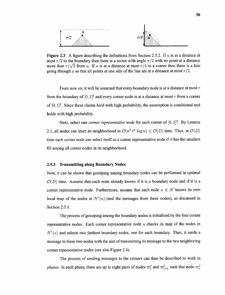
Figure 2.3 A figure describing the definitions from Section 2.5.2. If u is at a distance atmost r/2 to the boundary then there is a sector with angle 71/2 with no point at a distancemore than r/N/2 from u. If u is at a distance at most r/4 to a corner then there is a linegoing through u so that all points at one side of the line are at a distance at most r/2.

From now on, it will be assumed that every boundary node is at a distance at most r

from the boundary of [0, 11 2 and every corner node is at a distance at most r from a corner

of [0, 11 2 . Since these claims hold with high probability, the assumption is conditional and

holds with high probability.

Next, select one corner representative node for each corner of [0, 11 2 . By Lemma

2.l, all nodes can learn its neighborhood in 0(n2 r4 log n) < 0(D) time. Thus, in 0(D)

time each corner node can select itself as a corner representative node if it has the smallest

ID among all corner nodes in its neighborhood.

2.5.3 Transmitting along Boundary Nodes

Now, it can be shown that gossiping among boundary nodes can be performed in optimal

0(D) time. Assume that each node already knows if it is a boundary node and if it is a

corner representative node. Furthermore, assume that each node u E N knows its own

local map of the nodes in NT (u) (and the messages from these nodes), as discussed in

Section 2.5.1.

The process of gossiping among the boundary nodes is initialized by the four corner

representative nodes. Each corner representative node u checks its map of the nodes in

NT (u) and selects two farthest boundary nodes, one for each boundary. Then, it sends a

message to these two nodes with the aim of transmitting its message to the two neighboring

corner representative nodes (see also Figure 2.4).

The process of sending messages to the corners can then be described to work in

phases. In each phase, there are up to eight pairs of nodes -cu' and ail+1 such that node

31

Figure 2.4 Transmitting along boundaries.

wants to transmit a message to node wji+1, with both w and wji+1 being boundary nodes

and wji+1 E NT (wji). At the beginning of the phase, the node Si checks its local map and

finds a path from 771 to wji+1 of length at most T. Then, it transmits to its neighbors

and request that only the first node on P 3 will transmit the message to r4+1 . Then, the first

node on P3 will transmit to its neighbors and will request that only the second neighbor

on Pi, will transmit, and so on, until the node 74+1 will receive the message. Once wji+1

received a message, it sends back an acknowledgement to wji that the message has been

delivered. The algorithm for sending an acknowledgement is a reverse of the algorithm for

transmitting a message from 74 to z74+1 .

farthest from wji . As an exception, if one of the corner representative nodes is in NT (w,4 1 )\

{wji } , then this corner representative node is selected as wji+2 and then the process stops,

i.e., wji+3 will not be selected.

Obviously, if there are no transmission conflicts between the eight pairs wji and

then each phase can be performed in 27 - communication steps (including sending the

acknowledgement.) The only way of having a transmission conflict is that two pairs w .".

and wji+1, and wt and wji'+ 1, are transmitting along the same boundary and that in this

32

an acknowledgement. In this case, both wji and wji' repeat the process of transmitting their

messages to wji+1 and wji'+1 , respectively, using the selector approach from Lemma 2.1 that

ensures that the phase will be completed in 0(T • n2 r4 log n) = (9(D) communication

steps.

Therefore, each corner representative node will receive all messages from the

boundary nodes of its incident boundaries. If this process is repeated again, then each

corner representative node will receive the messages of all boundary nodes. If this process

is repeated once again, then all' nodes will receive the messages from all boundary

nodes. If now the approach from Lemma 2.1 is applied, then each boundary node will

receive a message from at least one', and hence it will receive messages from all

boundary nodes.

By the comments above, if there is no conflict in a phase, then the phase is

completed in 27- communication steps, but if there is a conflict, then the number of

communication steps in the phase is 0(T n2 r4 log n). If a corner representative node

originates a transmission that should reach another corner representative node, then there

will be at most a constant number of phases in which there will be a conflict. Therefore,

the total running time for this algorithm is 0(T • D/T) + 0(r n2 r4 log n) = 0(D).

Lemma 2.9 The algorithm above completes gossiping among all boundary nodes in 0(D)

time.

33

2.5.4 Gossiping via Transmitting along Almost Parallel Lines

Now, the result from Section 2.5.3 is extended to perform gossiping for the entire network

N. Assume that the algorithm from Section 2.5.3 has been completed and that each

boundary node knows all four corner representative nodes and knows their local maps of

all boundary nodes.

Let g be the corner representative node with the smallest ID. Let p* be the corner

representative node that shares the boundary with g (there are two such nodes) and that has

the smaller ID. Let g select O(D/T) boundary nodes CI, C2, ... such that

It is easy to see that such a sequence exists that g is able to determine the sequence

because after the gossiping process from Section 2.5.3, g knows all boundary nodes and

their τ neighbors. Next, g informs all boundary nodes about its choice using the process

from the previous section.

Now an algorithm in which all the nodes ςi will originate a procedureStraight-line

transmission aiming at disseminating the information contained by these nodes along a

line orthogonal to the boundary shared by g and 0* will be presented.

There are a few problems with this approach that need to be addressed. First of

all, the boundary of the unit square is unknown and instead, the goal will be to consider

lines orthogonal to the line r going through g and g*. The location of L can be determined

from the local map known to all the boundary nodes. Notice that since the angle between

the boundary of [0, 11 2 and G is at most 0(r), r is a good approximation of the boundary

of [0, 11 2 . Next, observe that one is not be able to do any transmissions along any single

line because the network N does not contain three collinear nodes with high probability.

Therefore, the process will need to proceed along an approximate line.

The following lemma is the key point to quantify the angle between the perfect line

to transmit along and the line along which to actually transmit.

34

Figure 2.5 Construction used in the proof of Lemma 2.10.

contained in [0, 1] 2 then with high probability there is a node w E N[T/4](u)) \ /N[T/8](u)

such that IL(luuw) < n -112 . The angle between lu and the line going through u and w is

at most n- 112 .

Proof: By Lemma 2.17 (an auxiliary lemma in Section 2.8), for every node z E S NT (u)

(e.g., with z being in the strict τth neighborhood of u), one has (1—o(1))•T•r < dist(u, z) <

T • r. One can proceed as depicted in Figure 2.5. Consider the area A which is the difference

of two disks centered at u, one of radius (1— ) • T • r/4 and another of radius (1 + ε) •T •r/8,

that is, A = B(u, (1 — ε) •T •r/4) \ B(u,(1 + ) •T •r/8).Here, it is assumed that ε is

a small positive constant such that all points in A belong to N[τ/4] (u) \ N[T /8] (u). (The

existence of ε follows from Lemma 2.17.)

Consider the sector S of angle n-1/2 with the center at u and with lu being its

bisector. The expected number of points in A is greater than n/polylog(n). Therefore, the

expected number of points in An S is w(n 1 /3 ). Hence, with high probability there is a node

in A n S, that yields the lemma. ❑

Straight-line Transmission Now, one can use Lemma 2.10 to design a scheme that

allows a point to transmit a message along an approximate line. The procedure Straight-line

transmission(s, p,, l) aims at transmitting a message it from node s along (approximately)

line ls , s E -es , so that all nodes that are close to ls will receive the message u.

35

In Straight-line transmission(s, ls), the node s initiates sending its message p,

along the line ls , u E ls . The transmission process is performed in phases; each phase

consists of sending a message from a node w i to another node wi+1 such that l s is

approximately equal to the line going through w i and wi+1, and wi+1 E NI[T/4] (ii)

N[T/8](wi). The nodes wi are determined recursively. Initially, 770 s and w 1 is the node

q E N[T/4] (s) \ N[T /8i (s) for which (l s sq) is minimized. If i > 1 and w i is determined,

then

(i) if NT (WO \ {wi-1} contains a boundary node then wi+1 is undefined and the

process is stopped; (ii) otherwise, w i+1 is selected to be the node u E N[T/4] (wi)

N[t/8](wi) for which IL (wi-1wiwi+i) — πI is minimized.

Since wi knows the locations of all nodes in NT (wi ), wi is able to select the node

wi+1 using its local map.

Before the running time of Straight-line transmission (s, ls) is analyzed, the

usage of this procedure is discussed first. Straight-line transmission(s, s ) will be called

with s being the nodes g, o*, and ς1, ς2, ., as defined at the beginning of Section 2.5.4,

and with line s being the line going through s that is orthogonal to the line .0 (which is the

line going through g and g*). (See also Figure 2.6).

the other hand, as it is argued above, every procedure Straight-line transmission(s, ,u, ls ) is

sending messages only among the nodes that are at distance at most n -1/3 from the line ls ,

where this claim holds with high probability. Therefore, in particular, the communication

in the calls to Straight-line transmission(s, p, ls) will be done without any interference

between the calls, with high probability.

36

Figure 2.6 e, i and g* do transmitting-along-a-line.

Now one can argue that each phase can be done in time 0(4 First, node s checks

its local map, chooses node w 1 , and selects a path from s to w 1 with 0(7) hops. Next, s

sends a message containing the message and the information about nodes on the selected

path from s to w1 . The first node on this path, say p i , is in N(s) and therefore it receives

the message in the first round. Then, in the second round only the node pi transmits and the

second node on the path, say 132 , will receive the message. Proceeding in this way, w1 will

receive the message in 0(7) steps. This establishes the running time of 0(7) for the first

phase; every other phase can be implemented in identical way. Since there are 0(D/7)

phases, this yields the following.

Lemma 2.11 All calls to Straight-line transmission(s, μ , l s) with s being g, g*, and

C2 . . . can be completed in 0(D) communication steps, with high probability.

Observe that while running the procedures Straight-line transmission, each node

that is transmitting can include in its message also all the knowledge it contains at a given

moment. Therefore, in particular, each last node W k will receive all the messages collected

on its path from s.

Next, observe that for every node q in the network AT either q has been selected as

one of the nodes w iin one of the calls to Straight-line transmission or one of the nodes in

NT (q) has. Indeed, since the distance between the adjacent lines ls is at most L7/4 • r,

for each point q E N there is a line Qs with dist(q, l s) ≤ [7/ 4 j • r/2. Therefore, by the

37

analysis of the procedure Straight-line transmission, there will be at least one node w i for

Straight-line transmission(s, lc , ls) with dist(q, ≤ 'r • r/2. And by Lemma 2.17, this

implies that wi E NT (q) with high probability.

Because of this, if all nodes u E Ai know the messages from all nodes in NT (u),

then after completing the calls to Straight-line transmission, for each node u E N there

will be at least one boundary node that received the message of u.

2.5.5 Gossiping Algorithm

The complete gossiping algorithm will be presented in this section. First run the algorithms

presented in Lemma 2.9, that perform gossiping among the boundary nodes. Afterwards,

all boundary nodes know all the messages from other boundary nodes and also know the

local maps with all boundary nodes. Next, run Straight-line transmission(s, s ) with s

being g, o*, and as discussed at the beginning of section 2.5.4. Then, as argued

at the end of Section 2.5.4, the boundary nodes will have the messages from all the nodes

in the network. Therefore, if one does gossiping among the boundary nodes (cf. Section

2.5.3) once again, then all the boundary nodes will have the messages from all the nodes

in N. Next, run again Straight-line transmission(s, μ, ls ) with s being g, o*, and si, C-21 • ••

Then, all the nodes wi will obtain the messages from all nodes in N. Finally, since each

q E N has in its τ-neighborhood a node wi , on can apply Lemma 2.1 to ensure that all

nodes in N. will receive the messages from all other nodes in N. Since the total number of

communication steps in the algorithm above is 0(D).

between a pair of nodes the node receiving the message is able to determine the distance

to the other node, then gossiping in a random geometric network can be completed in

deterministic time 0(D). The algorithm may fail with probability at most 1/n2 .

2.6 Deterministic Distributed Algorithm: Knowing Angles Helps

One can modify the algorithm from Theorem 2.12 to work in the scenario in which a

node cannot determine the distance between its neighboring node but instead, it is able to

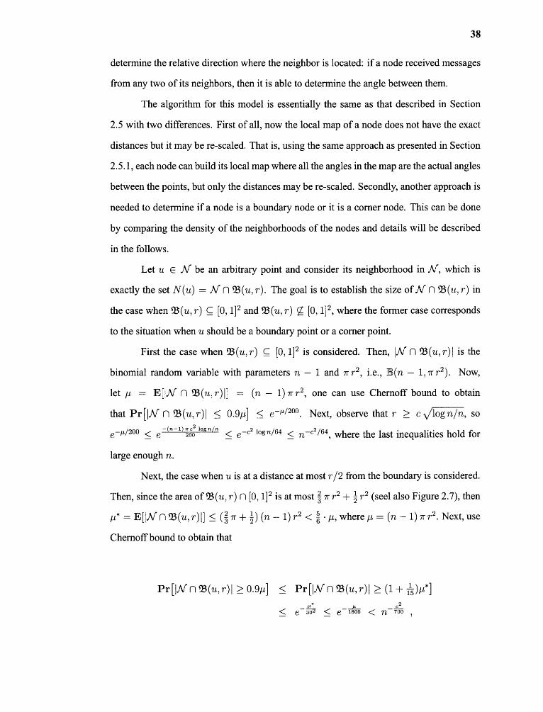
38

determine the relative direction where the neighbor is located: if a node received messages

from any two of its neighbors, then it is able to determine the angle between them.

The algorithm for this model is essentially the same as that described in Section

2.5 with two differences. First of all, now the local map of a node does not have the exact

distances but it may be re-scaled. That is, using the same approach as presented in Section

2.5.1, each node can build its local map where all the angles in the map are the actual angles

between the points, but only the distances may be re-scaled. Secondly, another approach is

needed to determine if a node is a boundary node or it is a corner node. This can be done

by comparing the density of the neighborhoods of the nodes and details will be described

in the follows.

Let u E N be an arbitrary point and consider its neighborhood in N, which is

exactly the set N(u) = N n B(u, r). The goal is to establish the size of N n B(u, r) in

the case when %(u, r) C [0, 11 2 and B(u, r) g [0, 112, where the former case corresponds

to the situation when u should be a boundary point or a corner point.

Figure 2.7 Ball B(u, r) for a point at a distance at most r/2 from the boundary.

where the last inequality uses the fact that r ≥ c \/log n/n and assumes that n is

sufficiently large.

Therefore, by the analysis, if c is sufficiently large, say c > 50, and a node u is

defined to be a boundary node if N(u) < 0.9p, then with high probability every node that

is at a distance at most r/2 from the boundary will become a boundary node and every

node that is at a distance larger than r from the boundary is not a boundary node. (See also

Figure 2.7.)

Corner nodes can be considered in the similar way. One can show that if c is a

sufficiently large constant then if a node u is defined to be a corner node when N(u) <

0.4,u, then with high probability every node that is at a distance at most r/10 from one of

the corners will become a corner node and every node that is at a distance larger than r

from the corners is not a corner node. (The constants are not optimized, which could be

easily improved.)

With these new definitions of boundary nodes and corner nodes, one can easily

convert the algorithm from Theorem 2.12 to obtain Theorem 2.13.

39

between a pair of nodes the node receiving the message is able to determine the relative

direction from which the message arrives, then gossiping in a random geometric network

40

can be completed in deterministic time 0(D). The algorithm may fail with probability at

most 1/n2 .

2.7 Conclusions

In this chapter the first thorough study of basic communication aspects in random geometric

ad-hoc radio networks is presented. It has been shown that in many scenarios, the

random structure of these networks (which often may model realistic scenarios from sensor

networks) makes it possible to perform communication between the nodes in the network

in asymptotically optimal time 0(D), where D is the diameter of the network and thus a

trivial lower bound for any communication. This is in contrast to arbitrary ad-hoc radio

networks, where deterministic bounds of o(n) are unattainable.

The study shows also that while there is a relatively simple optimal randomized

gossiping algorithm and a deterministic one when the nodes have knowledge about their

locations in the plane, the other scenarios are more complicated. In particular, it is still

unclear that if an 0(D)-time gossiping algorithm is possible in the unknown topology

model. But the algorithms from Sections 2.5 and 2.6 demonstrate that if the nodes can

obtain even a very limited geometric information about the neighbors, then some nice

algorithms can coupe with this task.

2.8 An Auxiliary Lemma (Lemma 2.17)

For any point q in R2, let (ix ) denote its x-coordinate and q(Y) denote its y-coordinate. For

any point q, a disc of q is the disc of radius r with the center at q. The right half-disc of q

is the set of all points in the disc of q whose x-coordinate is greater than or equal to q (x ) .

Similarly, the left half-disc of q is the set of all points in the disc of q whose x-coordinate

is smaller than or equal to q (Y ) .

Let p be any point in If8 2 and assume that it is in the origin. Define a sequence of

points X0 , X1 , ... as follows:

• X0 = p, and Xi is the neighbor of Xi-1.

Claim 2.14 For every i, point X i is in the ith neighborhood of p.

The following lemma is key for the analysis.

41

Figure 2.8 Description for the proof of Lemma 2.16.

Proof: Fix Xi and assume, without loss of generality, that Xi(x) < 0. Consider a sector

S of the disc of Xi of angle a as in Figure 2.8, with one boundary of the sector parallel to

the y-axis. Only the case when a = o(1) needs to be considered. If the other boundary

of the sector crosses the disc boundary at point q, then let 'T be the projection of q into the

y-coordinate. Let x = dist(Xi , 7). Notice that x = r • cos a and dist(T, q) = r • sin a.

Using Taylor's expansions, since a = o(1), x = r • (1 — (2 o(1)) • a 2 ) and dist(τ, q) =

42

Figure 2.9 Final location of point Xk.

r • (1 + o(1)) • a. Let C = S — ∆ (Xi , T, q); here ∆ (Xi,T, q) denotes the triangle on points

Xi, T, q.

Observe that Xj(Y)+1 — 4' ) is equal to the maximum value of x in Figure 2.8 for

which C is empty. Therefore, in order to estimate the value of E [X4. — Xi(y)IXi(y)] it is

enough to prove that if the angle a is chosen so that x = r (1 — 1/Θ(ln2/3 n)) then C will

contain at least one point with a (positive) constant probability, and if x is much bigger then

C contains no point.

Since the probability that C contains a point depends on the area of C, the goal is

to estimate the area of C. Clearly, dist(τ, q) • (r — x) < area(C) ≤ dist(τ, q) • (r — x).

Hence,

and similarly,

Therefore, area(C) = 0(r 2 • a3 ). For a = Θ(1/(n1/3r2/3) ), area((C) ≥ 1/n, in which

case, one will expect to see at least one point in C. Therefore, the expected value of

Now, it is not difficult to extend the result of Lemma 2.16 to the following.

43

2.9 Some Simulation Results of Randomized Algorithm (Section 2.2) and

Deterministic Algorithm (Section 2.3)

It has been proven theoretically that when r is not much greater than critical range,

both randomized gossiping algorithm and the deterministic algorithm finishes gossiping

in 0(D) rounds. But one may have noticed that the constant hidden behind the big 0

notation could be quite large. The simulation results reveal it is not the case. From Table

2.9 and Table 2.9, one can see that when r is near critical range, the randomized algorithm

works very fast, with a small constant factor (about 25). The deterministic algorithm runs

slightly faster since the location information is known (the constant factor is about 17).

As mentioned before, deterministic algorithm needs extra GPS devices and more resources

(memory, computation, bandwidth). In most cases, the randomized algorithm is the best

choise.

44

Table 2.1 Randomized Gossiping Algorithm. r = 2 x critical range. NR is the Number

n = 1000 2000 3000 4000 5000 6000 7000 8000 9000 10000

NR 510 640 698 790 897 993 1018 1101 1176 1265

NR/D 25.4 24.4 22.4 22.4 23.l 23.5 22.7 22.0 23.5 23.8

Table 2.2 Deterministic Gossiping Algorithm. r = 2 x critical range. NR is the Number of Rounds

n = 1000 2000 3000 4000 5000 6000 7000 8000 9000 10000

NR

NR/D

361

19.0

462

17.6

489

15.8

571

16.2

608

15.6

683

16.2

704

15.6

779

16.3

835

16.6

932

17.5

CHAPTER 3

COMMUNICATION PROBLEMS IN RANDOM LINE-OF-SIGHT AD-HOC

RADIO NETWORKS

3.1 Clarify of The Model: New Definition of Collisions

In a classic radio network, a node x gets the message from node y if and only if: (i) x does

not transmit (is in the listening mode) and (ii)yis the only neighbor ofxthat is transmitting

in that round.In the case that constraint (ii) is violated, a collision occurs, in which case no

message is received by x. In particular, it is assumed that x is unable to detect if a collision

happened or none of its neighbors did transmit.

In the classical radio network model a node cannot receive any message if more

than one of its neighbors transmits because the radio signals from these nodes will interfere.

Although this definition is often used to model radio ad hoc networks, this definition of the

collision here is too narrow to fit the framework of ad hoc networks in the line-of-sight

model. Since in a radio network messages are sent out via microwave signals, signals can

interfere each other if they overlap in space (rather than just by saying that when two or

more neighbors transmit). For example, in Figure 3.1, a sending node z can interfere the

node x from receiving the message of y, even though z is not the neighbor of x.

To cope with this phenomenon, one more constraint is added to ensure that node x

receives the message from y: (iii) no neighbor of y is transmitting and there is no node z

that is transmitting and that lies on a grid-line perpendicular to the segment Ty and is at a

distance at most r from the segment Ty, see, e.g., Figure 3.1. If either condition (ii) or (iii)

is violated, then a collision occurs. It is easy to see that any gossiping algorithm that works

in the new model will certainly work in the traditional model, but not vice versa.

3.2 Properties of Random Line-of-Sight Networks

Two parameters, r and p, play a critical role in the analysis of properties of the random

line-of-sight networks. Frieze et al. [Frieze et al. 2007] proved that when r = o(n) and

45

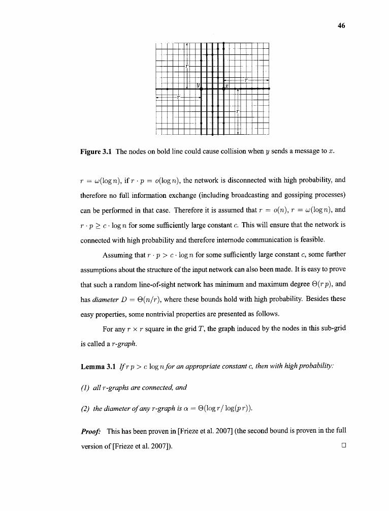
46

Figure 3.1 The nodes on bold line could cause collision when y sends a message to x.

r = w(log n), if r • p = o(log n), the network is disconnected with high probability, and

therefore no full information exchange (including broadcasting and gossiping processes)

can be performed in that case. Therefore it is assumed that r = o(n), r = w(log n), and

r • p ≥ c . log n for some sufficiently large constant c. This will ensure that the network is

connected with high probability and therefore internode communication is feasible.

Assuming that r • p > c . log n for some sufficiently large constant c, some further

assumptions about the structure of the input network can also been made. It is easy to prove

that such a random line-of-sight network has minimum and maximum degree 8 (r p), and

has diameter D = Θ(n/r), where these bounds hold with high probability. Besides these

easy properties, some nontrivial properties are presented as follows.

For any r x r square in the grid T, the graph induced by the nodes in this sub-grid

is called a r-graph.

Lemma 3.1 If r p > c log n for an appropriate constant c, then with high probability:

(1) all r-graphs are connected, and

Proof: This has been proven in [Frieze et al. 2007] (the second bound is proven in the full

version of [Frieze et al. 2007]). El

47

For simplicity of presentation, throughout the section the term a will be used as in

the lemma above.

All the claims in Lemma 3.1 hold with high probability, that is, with probability at

least 1 — 1/n 3 . Therefore, from now on, these events are implicitly conditioned on.

3.3 Preliminaries

Let V be the set of nodes in the grid. For any node x, define N(x) to be the set of nodes

that are reachable from x in one hop, N(x) = {y E V : dist(v, u) < r and x, y are on

the same straight line}, where dist(v, u) is the distance between v and u. Any node in

N(v) is called a neighbor of v, and the set N(v) is called the neighborhood of v. For

any X C V, let N(X) = UxEX N(x). Define the kth neighborhood of a node v, Nk (v),

recursively as follows: N° (v) = v and Nk (v) = N(Nk -1 (v)) for k ≥1.Let A be the

maximum degree and D be the diameter of the radio network. A = maxvev{IN(v)I} and

D = minvEv{k : Nk(v) = V} . As mentioned earlier, A = Θ(r p) and D = Θ(n/r), with

high probability.

Definition 3.2 (Collision sets) Let x, y E T with x E N(y). Define the collision set for the

communication from y to x, denoted by C(y, x), to be the set of nodes that can interfere x

from receiving a message from y. The set C(y, x) contains all nodes z E T that satisfy one

of the following:

1. z E N(x) U N(y), or

2. there is a grid point q such that (1) q lies on the segment connecting x and y, (ii) gridline -,q is orthogonal to the grid line Y g, and (iii) dist(z, q) ≤ r.

It is easy to see that C (y , x) = 0(r 2 p) with high probability.

By using the strongly selective family on line-of-sight networks (and for the new

notion of collision sets), one can get a similar lemma as Lemma 2.1. Since the proof of it

shares the same idea as the proof of the Lemma 2.1, the proof is omitted here.

Lemma 3.3 In random line-of-sight networks, for any integer k, in (deterministic) time

0(k r4 p2 log n) all nodes can send their messages to all nodes in their kth neighborhood.

48

The algorithm may fail with probability at most 1/n2 (where the probability is with respect

to the random choice of the nodes in the line-of-sight network).

The following is an immediate corollary of Lemma 3.3 obtained by setting k = D

(which corresponds to the bound from [Clementi et al. 2003] in current setting):

Since r p = C2 (log n), the running time of this algorithm is C2 (n log4 n) in the best

case, and thus it is superlinear. The goal of this chapter is to develop algorithms that are

faster, optimally, those that achieve the running time of the order of D, the diameter of the

network, which is a trivial asymptotic lower bound for broadcasting and gossiping.

3.4 Deterministic Algorithm with Position Information

The gossiping problem in random line-of-sight networks is considered in the model, where

each node knows its own geometric position in the grid. In such model, Dessmark and

Pelc [Dessmark and Pelc 2007] give a deterministic distributed broadcasting algorithm that

runs in (9(D) time. It can be applied to solve the broadcasting problem in the model of

this section, with the same running time. One can prove a similar result for gossiping by

extending the preprocessing phase from [Dessmark and Pelc 2007] and use an appropriate

strongly-selective family to collect information about the neighbors of each node.

Theorem 3.5 If every input node knows its location in the n x n grid, then the algorithm

Gossiping-Known-Locations-D below will complete gossiping in a random line-of-sight

network in deterministic time 0(a r4 p2 log n + n/r). The algorithm may fail with

probability at most 1/n2.

Figure 3.2 Horizontal and vertical segments.

algorithm achieves the asymptotically optimal running time of 0(D).

Here are some notations. First label the horizontal lines in the grid as H1, H2, ... ,

Hn from bottom to top; label the vertical lines in the grid as V 1 , V2, • • • , V. from left to

right. The crossing point of Hi and 17j is denoted as (Hi , Vj ). For each Hi , Hi is further

divide into segments of length of r/2, except for the last segment which is of length at

• • •most r/2, and label them as: Ho, H1 ,2, • • , Hi,[2n/r] from left to right. , ,vj,[2n/r]

is defined in a similar way, from bottom to top. See Figure 3.2.

49

50

It is easy to see that for r p > c log n with a sufficiently large c, with high

probability, there is a node in each segment. For any node x, define Mt (x) as the messages

known by x at step t. For any segment S, define Mt (S) as the common messages known

by all nodes in segment S at step t.

Proof: After the preprocessing in the algorithm Gossiping-Known-Locations-D, by

Lemma 3.3, every node knows which segment it belongs to, and every node knows all

other nodes in its segment, including their messages and positions. Therefore, in every

segment, all the nodes from that block can select a single representative who will be the

only node transmitting (for the entire segment) in all the following time slots.

Call all nodes that are scheduled to send by the algorithm representative nodes. By

the definition of the segment, in any time slot, when a segment (its representative) sends a

message, the nearest sending segment is at a distance of 2 r from it. So, after each sending,

the sending segment, say H i will successfully send its message Mt (Hi ,j ) to segments

Hi,- 1 and Hi ,j+1 if there are such segments. The statement is also true for any segment

Vi ,j . For any two nodes v and u in the grid, the algorithm will send the message of u to v

successfully: There are two representative nodes that are within the r x r square centered

51

at u and v respectively, with high probability. After preprocessing, the message of u will

be sent to its representative node. Then, after 0 (n/r) steps, the message of u will be sent

to the representative node of v. After the postprocessing, the message of u will eventually

reach v.

By Lemma 3.3, the running time of the preprocessing step is 0(a r4 p2 log n), and

the running time of the postprocessing phase is also 0(a r4 p2 log n\ .) Therefore, the total

running time of the algorithm Gossiping-Known-Locations-D is 0(a r4 p2 log n + n/r). ❑

3.5 Broadcasting and Deterministic Gossiping with a Leader

A more natural model is considered in this section in which each node knows the values of

n, r, and p, knows its own ID (which is a unique integer bounded by a polynomial of n), but

it is not aware of any other information about the network. In particular, the node does not

know its own location. This is the main model for the study of principles of communication

in random line-of-sight networks.

It is helpful to start with a slightly relaxed model: there is a special node (leader) f

in the network, such that ℓ knows that she is the leader, and all other nodes in the network

know that they are not the leader. It can be shown that in this model distributed gossiping

can be done deterministically in time 0 (a r4 p2 log n + n/r). This will immediately imply

a deterministic distributed broadcasting algorithm with asymptotically the same running

time.

The same preprocessing as that used in algorithm Gossiping-Known-Locations-D

from Section 3.4 is executed first. This takes 0(a r4 p2 log n)) steps. After the

preprocessing, each node knows its second neighborhood with high probability.

3.5.1 Gossiping along a Grid Line

First, gossiping among the nodes belonging to the same grid line can be performed in

optimal (9(1/r) time if there is a leader on the grid line.

The following two lemmas that estimate the size of the common neighborhood in

random line-of-sight networks can be easily derived from Chernoff bounds.

52

Lemma 3.6 For any pair of nodes u and v belonging to the same grid line, with high

probability:

Lemma 3.7 For any node u, if the distance between u and the nearest boundary is greater

than or equal to r, then, in each of the four directions, with high probability, there is a

neighboring node v of u such that 1.2 r p ≤ IN (u) n N(v) I ≤ 1.3 r p.

Proof Fix a node u and one direction. It is easy to see that with high probability, there is

a node v such that 0.74 r < dist(u,v) < 0.76 r. 1.24 r p < E[IN(u) n N(v)I] ≤ 1.26 r p.

Similarly as in the proof of Lemma 3.6, one can show that the following holds with high

probability: 1.2 r p < IN (u) fl N(v) < 1.3 r p. ❑

The process of gossiping among the nodes on a grid-line is initialized by one

specific node (call it a launching node). The launching node u checks its second

neighborhood N2 (u), and selects one representative node, say v, such that 1.2 r p ≤

IN (u) fl N (v)1 ≤ 1.3 r p. Then, u sends a message to v with the aims: (1) u transmits

53

its message to v and (ii) u informs v that it is picked as representative node. Because of

Lemmas 3.6 and 3.7, r/2 < dist(u, v) ≤ r.

The process of gossiping along a grid line works in steps. At the beginning of

each step, a node 'cut receives a message from node w t- 1 , and wt is informed that it is the

representative node. Then wt will pick a representative node wt+1 for the next step, and

then send a message to wt+1 to inform about it. w t picks wt+1 by checking N2 (cut ), and

selecting as wt+1 any node fulfilling:

Because of Lemmas 3.6 and 3.7, it is easy to see that r/2 < dist(wt+1 , Wt) ≤ r.

Moreover, wt+1 and wt-1 are at different sides of wt , for otherwise dist(wt+1, < r/2

and then the second constraint would be violated with high probability. If in one step wt

is unable to find the wt+1 as defined above, then the distance between Wt and its nearest

boundary is less than r. In that case wt simply stops the process and makes itself as the last

representative node.

This process is run for 2 n/r steps and the steps spent in this process is called Phase

1. Then the last representative node, say w t+1 , picks as next representative node and

initialize the process again, for another 2 n/r steps. These steps define Phase 2. Then,

the representative nodes in Phase 2 send their messages in reverse order and with that the

gossiping along straight-line will be done. These steps form Phase 3. The total running

time is O(n/r).

3.5.2 Broadcasting and Gossiping with the Leader in the Whole Grid

The gossiping algorithm in the model with a distinguished leader will be presented in

this section. First, the leader will pick an arbitrary direction and do gossiping along the

corresponding grid line. As a by product of this algorithm, a set of representative nodes

will be chosen and the minimum distance between any pair of them is greater than or

equal to r/2. Next, each of the representative nodes treat itself as the pseudo-leader, and

54

do gossiping along a grid line in parallel, in an orthogonal direction to that first chosen

by the leader. There are two issues to be solved. First, since the distance between these

pseudo leaders could be as small as r/2, one can interleave the transmissions in adjacent

pseudo-leaders, which yields a constant-factor slow-down. Second, by checking its second

neighborhood, a pseudo-leader can indeed find a node in orthogonal direction that was

first chosen by the leader. (w i can pick a node y from its neighbors such that 1.2 r p ≤

Next, the whole process is repeated (starting from the first gossiping along a grid

line initialized by the leader) once again. It is easy to see that gossiping is done among all

representative nodes. For any pair of nodes u and v, there are two representative nodes that

are within the r x r squares centered at u and v respectively, with high probability. After

preprocessing, u will send its message to its representative nodes. The message of u then

will be sent to the representative node of v in the following steps. Next the postprocessing

defined in the algorithm of the Section 3.4 will be run, and the message of u will be sent to

v. The running time is 0(a 7-4 p2 log n + n/r).

Theorem 3.8 If there is a leader in the random line-of-sight network, then gossiping can

be completed in deterministic time 0(a r4 p2 log n + n/r). The algorithm may fail with

probability at most 1/n2 .

Since in the broadcasting problem, there always is a given source node which can

be used as a leader, Theorem 3.8 immediately implies that broadcasting can also be done

in the same time.

Theorem 3.9 (Deterministic broadcasting) Distributed broadcasting in random line-of-

sight networks can be performed in deterministic time 0(a r4 p2 log n + n/r).

3.6 Fast Distributed Randomized Gossiping

The model of random line-of-sight networks in which each node knows the values of n, r,

and p, knows its own ID, but it is not aware of any other information about the network is

studied in this section. As one has seen in the previous section, if the nodes in the network

55

can elect a leader then gossiping could be done within the time bounds stated in Theorem

3.8. The problem of leader election is difficult in current setting, but as it will be shown in

this section, randomized leader election can be solved efficiently.

At the beginning, each node independently and uniformly at random selects itself

as the leader with probability logn/n2p. By simple probabilistic arguments, one can prove that

exactly Θ(log n) leaders are chosen with high probability. Then a distributed minimum

finding algorithm can be executed to eliminate all of them but one, and the one chosen will

have the lowest ID.

Each of these leaders will pick four representative nodes along four directions,

respectively, and execute the process of Phase 1 as described in Section 3.5.l. It can be

called fast transmission. The fast transmission can be interleaved with the preprocessing

of the algorithm in Section 3.4, that is called slow transmission. In the odd steps, every

node follows the schedule of fast transmission, and in the even steps, every node follow

the schedule of slow transmission. Since there is more than one leader, it is possible

that transmission collisions can occur. These collisions are able to be detected, because

after wt picks wt+1 as the next representative node and informs it, in the next step, wt is

expected to receive an acknowledgement of the successful transmission from wt+1. If the

acknowledgement is not received, wt knows that a collision happened.

When a node, say u, detects a collision, in the following 0 (a r4 p2 log n) steps u

will send nothing (stay in the listening mode) in odd steps, and run slow transmission as

before in even steps. By the property of strongly selective family, u will eventually receive

the messages of other representative nodes that are transmitting for their own leaders during

this period. Then u compares the ID of its own leader with all other leader's ID that it just

received. If (at least) one of those ID is smaller than the ID of its leader, u will send

an "eliminating" message back to its leader, reversely along the path through which the

leader sent the message to it. The leader eliminates itself after getting this message. If

the ID of u's leader is the smallest one, u resumes the fast transmission. Altogether, a

node will encounter at most O(log n) collisions when it transmits toward any boundary.

56

I Therefore the slow down caused by collisions is small and the total running time is

0(r4 p2 a log2 n + n/r).

Now the leader is either eliminated or successfully transmits its ID along four

directions. Thus, for any pair of surviving leaders, there is a pair of representative nodes in

one r x r square. By running the postprocessing from Section 3.4, the two representative

nodes will exchange information about their leaders. Again, the representative node that

holds the larger ID will transmit an "eliminating" message to its leader. The running time

is 0(r4 p2 a log2 n + n/r). After this procedure, all but one leader with the smallest ID

will survive.

Summarize the result above:

Theorem 3.10 In the random line-of-sight network, there is a distributed randomized

algorithm that finds a single node which is approved by all the nodes in the network as a

leader, and which completes the task in time 0(r4 p2 a log2 n + n/r), with high probability.

Finally, Theorem 3.10 with the result from the previous section can be combined

with Theorem 3.8, to obtain the following result.

Theorem 3.11 (Randomized gossiping) In the random line-of-sight network, distributed

gossiping can be done in randomized time 0(r4 p2 a log2 n + n/r), with high probability.

3.7 Conclusions

Three efficient algorithms are presented for broadcasting and gossiping in the model of

random sight-of-line networks. If r = 0(n'/5 / log3/ 5 n), then all algorithms perform 0(D)

steps to complete the task, which is clearly asymptotically optimal. While it is certainly

very interesting to extend the optimality of these bounds to larger values of r and this is

an interesting open problems of extending the results in this chapter to larger values of

r or providing lower bounds for the running times for larger values of r, it is believed

1It seems that if two nodes with distance less than or equal to r send along the same direction, thereare a lot of collisions. But in this case, both nodes will notice the collision at once, so after waitingfor 0(a r4 p2 log n) steps, the one with small ID will stop transmitting.

57

that the case r = 0(n 1 /5 / log3/5 n) covers the most interesting cases, when the graph is

relatively sparse and each node is able to communicate only with the nodes that are not

a large distance apart. Therefore, the most interesting specific open problems left in this

dissertation is to extend the result from Section 3.6 to obtain a distributed deterministic

algorithm for gossiping. Even more interesting is a more general question: what are the

important aspects of random sight-of-line networks to perform fast communication in these

networks. The work in this dissertation is only the very first step in that direction.

CHAPTER 4

ONLINE SCHEDULING OF EQUAL-PROCESSING-TIME TASK SYSTEMS

4.1 The 3/2 Bound

In this chapter it will be shown that Hu's algorithm yields a competitive ratio of 3/2 for the

problem P pj = 1, intree i released at time ri I Cmax; i.e., Cmax (S) < (3/2) *Cmax (S* ),

where S is the schedule produced by the online version of Hu's algorithm and S* is the

optimal (offline) schedule.

It is well known that Hu's algorithm is optimal for P pj = 1, intree Cmax .

It works by first assigning a label to each task which corresponds to the priority of the

task; tasks with higher labels have higher priority. Once the labels are assigned, the tasks

are scheduled as follows. Whenever a machine becomes free for assignment, assign that

task all of whose predecessors have already been executed and which has the largest label

among those tasks not yet assigned. In Hu's algorithm, the label of a task is a function of

the level of the task.

Definition 4.1 The level of a task i with no immediate successor is its processing time pi .

The level of a task with immediate successor(s) is its processing time plus the maximum

level of its immediate successor(s).

Hu's labeling algorithm assigns higher labels to tasks at higher levels; ties can be

broken in an arbitrary manner.

For any instance of P I pj = 1, intree Cmax, let SHu denote the schedule produced

by Hu's algorithm. Suppose that in SHE , the first t (t ≥ 1) columns are all full columns

(i.e., time units during which all machines have been assigned), but the (t + 1)' column is

a partial column (i.e., time unit during which some machines(s) are idle). Then it is easy

to see that all the columns after the (t + 1)' column are also partial columns. For any task

in the time interval [t, t + 1], if it has no predecessor in the first t columns, then it can be

moved backward to the time interval [0, 1] and the moving distance of this task is t, which

58

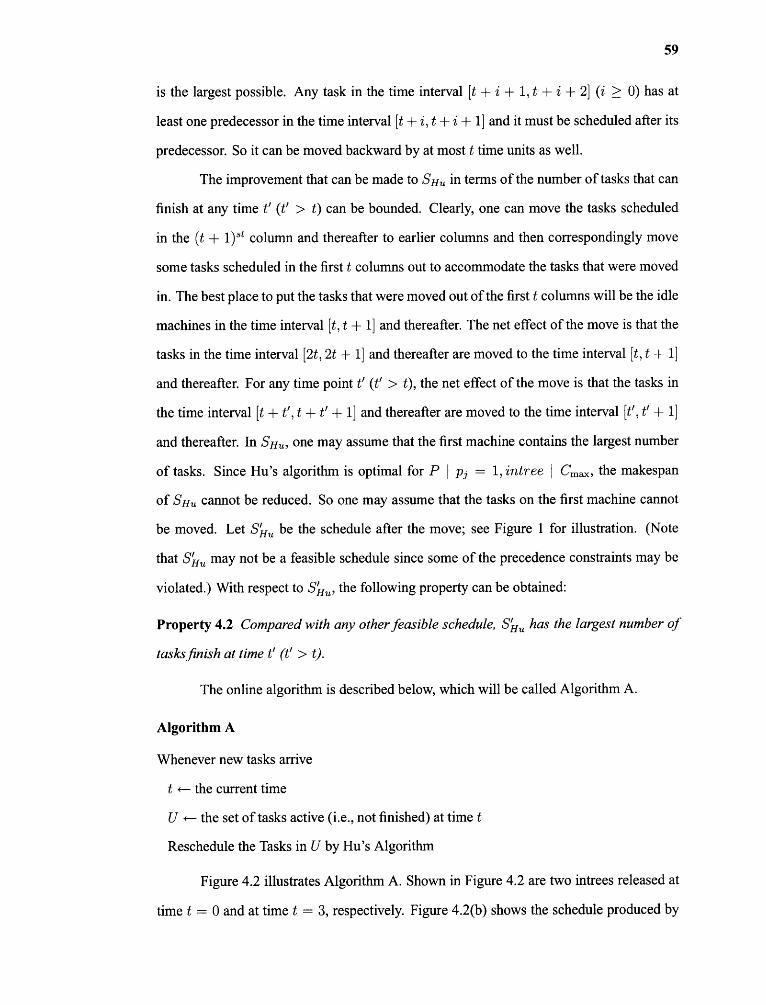
59

is the largest possible. Any task in the time interval [t + i + 1, t + i + 2] (i ≥ 0) has at

least one predecessor in the time interval [t + i, t + i + 1] and it must be scheduled after its

predecessor. So it can be moved backward by at most t time units as well.

The improvement that can be made to SHu in terms of the number of tasks that can

finish at any time t' (t' > t) can be bounded. Clearly, one can move the tasks scheduled

in the (t + 1)' column and thereafter to earlier columns and then correspondingly move

some tasks scheduled in the first t columns out to accommodate the tasks that were moved

in. The best place to put the tasks that were moved out of the first t columns will be the idle

machines in the time interval [t, t + 1] and thereafter. The net effect of the move is that the

tasks in the time interval [2t, 2t + 1] and thereafter are moved to the time interval [t, t + 1]

and thereafter. For any time point t' (t' > t), the net effect of the move is that the tasks in

the time interval [t + t' ,t + + 1] and thereafter are moved to the time interval [t', + 1]

and thereafter. In SHu, one may assume that the first machine contains the largest number

of tasks. Since Hu's algorithm is optimal for PI pj = 1, intree I C max , the makespan

of SHu, cannot be reduced. So one may assume that the tasks on the first machine cannot

be moved. Let S'Hu be the schedule after the move; see Figure 1 for illustration. (Note

that S'Hu may not be a feasible schedule since some of the precedence constraints may be

violated.) With respect to S'Hu , the following property can be obtained:

Property 4.2 Compared with any other feasible schedule, S'Hu has the largest number of

tasks finish at time t' (t' > t).

The online algorithm is described below, which will be called Algorithm A.

Algorithm A

Whenever new tasks arrive

t 4— the current time

U <— the set of tasks active (i.e., not finished) at time t

Reschedule the Tasks in U by Hu's Algorithm

Figure 4.2 illustrates Algorithm A. Shown in Figure 4.2 are two intrees released at

time t = 0 and at time t = 3, respectively. Figure 4.2(b) shows the schedule produced by

60

Figure 4.2 An example illustrating algorithm A.

Algorithm A at time t = 0, and Figure 4.2(c) shows the schedule produced by Algorithm

A at time t = 3.

For any instance of P pj = 1, intree i released at time ri Cm , let S denote

the schedule produced by Algorithm A, and let S* denote the optimal (offline) schedule.

Without loss of generality, one may assume that in S, the number of tasks on the jth

machine is greater than or equal to the number of tasks on the (j + I)' machine. If not, one

can relabel the machines. Assume that the first release time is r 1 and the last release time is

rk . Without loss of generality, one may assume that r1 = 0. The following two cases will

be considered.

61

1. All the machines are full in the time interval [0, rk ].

2. There are some idle machines in the time interval [0, rk ].

These two cases are considered separately in Sections 4.1.1 and 4.1.2, respectively.

4.1.1 Case 1

Let t be the last time instant such that there is a chain, say CH, of tasks scheduled in the

time interval [t,Cmax(S)], and Tt is the task scheduled in the time interval [t, t + 1] of which

no predecessor is scheduled in the time interval [t — 1, t]. Assume chain CH belongs to

intreej , its release time is r j , and it has c tasks (i.e., c = Cmax (S) — t). Furthermore,

assume the level of Tt is h.

Two cases are considered. The first case is when t = while the second case

is when t > rj . In the former case, it is easy to see that Cmax (S) cannot be reduced.

Thus, S is an optimal schedule. In the second case, if all the tasks scheduled in the time

interval [0, t] have levels at least h, then Cmax (S) cannot be reduced and hence S is again

an optimal schedule. However, if some tasks scheduled in the time interval [0, t] have levels

less than h, then it is possible to move these tasks to later time, and execute the chain CH

earlier. Consequently, Cmax (S) can be reduced. In the following the case where some tasks

scheduled in the time interval [0, t] have levels less than h is considered. See Figure 4.3 for

illustration.

From time 0, let t it be the first time instant such that there is at least one task with

level less than h executing in the time interval [4 1 , tit + 1].

From time 4 1 on, let t31 be the first time instant such that all the tasks executing in

the time interval [t j1 , tj1 + 1] have levels at least h; see Figure 3 for illustration. Let k 1 be

the number of tasks with levels at least h executing in the time interval [t j1 — 1, tj1 ]. So

1 ≤ k 1 < m — 1. Let F 1 be all the tasks released prior to tj 1 , but have not yet been executed.

Let 6 1 be all the tasks in F 1 that have levels at least h, and let Ψ1 C e l be all the tasks

that are ready for execution at time t31 (i.e., all of whose predecessors have been executed

by time tj1 ). Since in an intree any task has at most one successor, the number of tasks in

62

Figure 4.3 Some tasks scheduled in [0, t] with levels < h.

T 1 is at most k1 . Therefore, at most k 1 * 4 1 tasks in 6 1 can be scheduled before tj1 and the

k1 * tit tasks executed prior to 4 1 can replace the tasks with level less than h executing in

the time interval [4 1 , tj1 ]; see Figure 1 for illustration. The tasks that are replaced will be

scheduled at a later time.

From time tj1 on, let 4 2 be the first time instant such that there is at least one task

with level less than h executing in the time interval [tie, tie + 1].

From time 42 on, let t32 be the first time instant such that all the tasks executing

in the time interval [tj2, tj2 + 1] have levels at least h. Let k2 be the number of tasks with

levels at least h executing in the time interval [tj2 — 1, tj2]. So 1 ≤ k2 ≤ m — 1. Let F2 be

all the tasks released prior to tj2 , but have not yet been executed. In F2, if there are tasks

that belong to 1' 1 and that can be scheduled prior to tj1, remove these tasks from 1'2 . Let

02 be all the tasks in 1' 2 that have levels at least h, and let 111 2 C 02 be all the tasks that are

ready for execution at time t j2 . Since in an intree any task has at most one successor, the

number of tasks in 1112 is at most k2 . Therefore, at most k2 * (42 — tj1) tasks in 02 can be

scheduled before t 32 and the k2 * (42 — tj 1 ) tasks executed prior to 4 2 can replace the tasks

with level less than h executing in the time interval [42, tj2]. The tasks that are replaced

will be scheduled at a later time.

63

Continue to find [43 , t33], • • • , [tit, tjl] until time t. Let k3 , • • • , lc/ be defined as

before. Assume before t, there are a total of a columns that contain only tasks with level

at least h and there are a total of b columns that contain tasks with level less than h. The

number of tasks with level less than h that can be replaced is at most

If R is the number of tasks with level less than h that can be replaced, then the chain C can

be moved earlier by at most R/m time units, and the tasks that have been replaced can be

moved to the idle machines in the time interval [t — R/m,t — R/m — 1] and thereafter.

Consequently, a better schedule than S with a reduced Cmax can be obtained.

Now, Cmax (S) = a + b + c. If a > b, then there are at most

tasks with level less than h, and hence the chain CH can be moved earlier by at most b

time units. Therefore,

and

Hence,

On the other hand, if a < b, then at most a * m tasks with level less than h can be

replaced and hence the chain CH can be moved earlier by at most a time units. Therefore,

Cmax (S*) ≥ b + max{a, c}

Hence,

From the above discussions, the following lemma can be obtained.

Lemma 4.3 If there is no idle machine in the time interval [0, r id, then Cmax (S) < (3/2) *

Cmax (S* ).

4.1.2 Case 2

The basic idea in proving the worst-case bound is to convert the schedule S into a

new schedule S', which has a smaller Cmax than S* but may violate some precedence

constraints. If one can show that Cmax(S)/Cmax(S') < 3/2, then Cmax (S)/Cmax (S*) <

3/2 can be immediately obtained. The conversion is done by a sequence of conversions,

eventually arriving at the schedule S'.

Starting from time r 1 , let ri1 be the first release time such that there are some partial

columns or there is a level 1 task scheduled before ri1 in S. Let A be the schedule produced

by Algorithm A for the intrees released from the first i t — 1 release times only; see Figure

4.4 for an illustration. The improvement that can be made to S 1 in terms of the number of

tasks that can finish by ri1 can be bounded.

One can first examine the improvement that can be made to the Cmax of S. In

the last time instant t 1 such that there is a chain, say CHI , of tasks executing in the time

interval [t1, Cmax (Si )] is located. Let Tt1 be the head of the chain executing in the time

interval [t 1 , t 1 + 1] of which no predecessor is executing in the time interval [t 1 — 1, t 1 ], and

let the level of Tt1 be h1. Let ail be the total number of columns before t i during which

all the tasks executing have levels greater than or equal to h 1 , bi1 be the total number of

64

65

Figure 4.4 Illustrating the conversion process.

columns before t 1 during which some tasks executing have levels less than h 1 , and ci1 be

the length of the chain CH1 (i.e., ci1 = Cmax(S1) — t 1 ). From Case 1 in Section 4.1.l, the

Cmax of S1 can be reduced by at most min{a i1 , bi1 , ci1 }.

Now check the improvement that can be made in terms of the number of tasks that

can finish by ri1 . In the time interval [r1 , ri1 ], let F1 be the set of full columns in which

there is no level 1 task executing, and P 1 be the set of remaining columns. Let f i :=1 F1 I.

One can assert that min{a i1 , bi1 , ci1 } ≤ fi/2. For if h 1 < 1, then bi1 = 0 and hence

min{ai1 , bi1 , ci1 } = 0 ≤ f1 /2. On the other hand, if h 1 ≥ 2, then a i1 + bi1 ≤ f1 and hence

min{ a i1 , bi1 , ci1 } ≤ /2. For any task T executing in the time interval [ri1 , ri1 + 1], some

predecessor of T must be executing in some column of P1 . Since in an intree any task has

at most one successor, the tasks executing in the time interval [ri1 , ri1 + f1] can possibly

finish by time ri1 ; see Figure 1 for illustration. In S 1 , one may assume that the first machine

contains the largest number of tasks, compared with any other machines. Since the C max

of Ŝi can be reduced by at most min{a i1 , bi1 , ci1 } , one may assume that the tasks executing

66

in the time interval [ri 1 , ri1 + min {a i 1 , bi1 , ci1}] on the first machine can finish by ri1. Let

V1 be the set of tasks executing in the time interval [ri1, ri1 + min{ a i1 , bi1 , ci1 }] on the first

machine plus all the tasks executing in the time interval [ri1, ri1 + fi ] on the other m — 1

machines.

All the precedence constraints related to the tasks in V 1 are removed and the tasks

are moved to the idle machines before ri1 . The movement is stopped as soon as all the

machines before ri1 are full. Let V1 be the remaining tasks in Vi . Now a new schedule S1

from S1 is obtained. By the discussions before, S1 has the largest number of tasks finish by

ri1,compared with any other feasible schedule for the intrees released from the first ii— 1

release times.

Now S can be converted into a new schedule S1 as follows. In Si , the schedule

in the time interval [r1 , ril l is identical to that of the schedule Si . The remainder of the

schedule is obtained as follows. Let TS]. be the task system consisting of all the tasks in

VI', all the tasks that have not yet been scheduled by time ri1 from the intrees released from

the first i i —1 release times, and all the intrees released at or after ri1 up to and including rk .

Call Algorithm A to schedule the tasks in TS1, starting at time ri1. The schedule obtained

by Algorithm A will be the remainder of S1 .

S1 can be converted into a new schedule S2 by the same procedure as above.

Starting from ri1, let rig be the first release time such that there are some partial columns or

there is some level I task scheduled before rig in Si . Let S2 be the schedule produced by

Algorithm A for the tasks in V1, all the tasks that have not been scheduled by ri 1 from the

intrees released from the first i i — 1 release times, and all the intrees released at or after ri1

but before rig . The schedule S2 starts at time ri1. The improvement that can be made to S2

in terms of the number of tasks that can finish by r ig can be bounded.

In S2, let t2 be the last time instant such that there is a chain, say CH2 , of tasks

executing in the time interval [t2 , Cmax(Ŝ2 )]. Let Tt2 be the head of the chain executing

in the time interval [t2 , t2 + 1] of which no predecessor is executing in the time interval

[t2 — 1, t2 ], and let the level of Tt2 be h2 . Let ail be the total number of columns before t 2

during which all the tasks executing have levels greater than or equal to h2 , bi2 be the total

67

number of columns before t 2 during which some tasks executing have levels less than h 2 ,

and ci2 be the length of the chain CH2 (i.e., c22 = Cmax (S2 ) — t2 ). From Case 1 in Section

2.1, the C. of S2 can be reduced by at most min{a i2 , bit , ci2 }.

Consider the improvement that can be made in terms of the number of tasks that can

finish by rig . In the time interval [ri1 , ri2 ], let F2 be the set of full columns in which there

is no level 1 task executing, and P2 be the set of remaining columns. Let f2 = 1 F2 1' By

the same reasoning as above, it can be shown that min{ai2, bit , c,2} ≤ f2 /2. For any task

T with level greater than 1 executing in the time interval [rig , rig + 1], some predecessor

of T must be executing in some column of P2. Since in an intree any task has at most one

successor, the tasks executing in the time interval [r,2 , ri2 + f2 ] can possibly finish by time

ri2 ; see Figure 1 for illustration. In S2, one may assume that the first machine contains

the largest number of tasks, compared with any other machines. Since the C. of S2 can

be reduced by at most minfai2 , bi2 , ci2 }, one may assume that the tasks executing in the

time interval [rig , ri2 + min{ai2 , bi2 , ci2 }] on the first machine can finish by time r,2 . Let

V2 be the set of tasks executing in the time interval [ri2 , ri2 + min{ a, 2 , bi2 , ci2 }] on the first

machine plus all the tasks executing in the time interval [ri2 , ri2 + f] on the other m — 1

machines, but not in V1 .

All the precedence constraints related to the tasks in V2 are removed and these tasks

are moved to the idle machines before ri2 . The movement is stopped as soon as all the

machines before r, 2 are full. Let 17 be the remaining tasks in V2 . Now a new schedule S2

from S2 is obtained. By the discussions before, S2 has the largest number of tasks finish by

ri2 , compared with any other feasible schedule for the intrees released between r i1 and rig

plus the remaining tasks from the intrees released from the first i t — 1 release times.

Now S1 can be converted into a new schedule S2 as follows. In S2, the schedule in

the time interval [r1 , ri1 ] is identical to that of the schedule S1 . The schedule in the time

interval [ri1 , ri2] is identical to that of the schedule S2. The remainder of the schedule is

obtained as follows. Let TS2 be the task system consisting of all the tasks in W, all the

tasks that have not yet been scheduled by time ri2 from the intrees released prior to ri2 , and

all the intrees released at or after r i 2 up to and including rk. Call Algorithm A to schedule

68

the tasks in TS2 , starting at time rig . The schedule obtained by Algorithm A will be the

remainder of S2.

One can repeat the above process until the schedule S y is obtained such that in Sy ,

there is no partial column and there is no level 1 task scheduled before rk . Let Ŝy+1 be

the portion of the schedule Sy in the time interval [r iy , Cmax (Sy )]. Clearly, Ŝy+1 belongs to

Case 1 in Section 2.1. In let ty+1 be the last time instant such that there is a chain,

say CHy+1 , of tasks executing in the time interval [t y+ 1, Cmax (Ŝy+1)]• Let Tt(y+1) be the

head of the chain executing in the time interval [t y+1 , ty+ 1 + 1] of which no predecessor

is executing in the time interval [t y+1 — 1, ty+1], and let the level of Tt(y+1) be hy+1. Let

aiy+1 be the total number of columns before t y+1 during which all the tasks executing have

levels greater than or equal to hy+1, bi y+1 be the total number of columns before ty+1 during

which some tasks executing have levels less than h y+i , and ciy+ 1 be the length of the chain

CHy+1 (i.e., ciy+1 = Cmax(Ŝy+1) — ty+1). From Case 1 in Section 2.1, the Cmax of Ŝy+1

can be reduced by at most min{a iy+ 1 , biy+1 , ciy+1 }.

From riy on, let t' be the first time instant such that in the time interval [t', t' + 1]

there is an idle machine or there is a level 1 task scheduled. Let fy+1 = t' — riy . Using the

same reasoning as above, it can be shown that min{a iy+1, bi y+1 , ciy+1 } ≤ 4+1/2 .

Let Vy+1 be the set of tasks executing in the time interval [t', t'+

min{aiy+1, biy+1 , ciy+1}] on any machine. Move the tasks in Vy+1 to the idle machines

in the time interval [t', t' + 1] and thereafter. Finally, move the tasks from time t' +

min{aiy+ 1 , biy+ 1 , ciy+1 } until time Cmax(Ŝy+i) backwards by min{a iy+ 1 , biy+1 , ciy+ 1 } time

units. The new schedule will be called Sy+1.

Now Sy can be converted into a new schedule S' as follows. In S', the schedule in

the time interval [r i , riy ] is identical to that of Sy , while the schedule in the time interval

[riy , Cmax (Sy+i )] is identical to that of Sy+1 . In the next lemma, it will be shown that S'

has a smaller Cmax than S*.

Lemma 4.4 S' has a smaller Cmax than S*.

69

Proof By converting the schedule S into the schedule Si , a new task system TS1 is

obtained. TS1 contains the tasks from the intrees released in the first i t — 1 release times

that have not yet been executed by ri1 in Si , plus all the intrees released at or after ri1. Let

OPT1 be the optimal schedule for TS1 . The claim is that ri1 + Cmax(OPT1 ) ≤ Cmax (S* ).

From S*, all the tasks from the intrees released in the first i t — 1 release times are

deleted, and the portion of the schedule in the time interval [r1,ri1] is replaced by Si . Let

the resulting schedule be S. Now fill the idle machines after time ri1 in S by the tasks from

the intrees released in the first i t — 1 release times (that have not yet been executed by the

time ri 1 in Si ). Since S1 has the largest number of tasks finished at time ri1 the total idle

time in S is larger than or equal to the number of tasks from the intrees released in the first

it — 1 release times. Since all other tasks with levels greater than 1 and their successors in

T51 , with the exception of the tasks in VI, cannot finish before ri1, these tasks in T51 can be

filled into the idle machines as they are scheduled in S*, and the remaining tasks in the idle

machines in S* can be filled in an arbitrary manner. Thus, ri1 + Cmax(OPT1) ≤ Cmax (S*).

Similarly, after converting the schedule S 1 into the schedule S2, a new task system

TS2 is obtained. Let OPT2 be the optimal schedule for TS2. Then rig + Cmax(OPT2) ≤

ri1 + Cmax(OPT1) ≤ Cmax (S*). Finally, Cmax (S') ≤ riy + Cmax (OPTy ) ≤ Cmax (S*). ❑

Now Cmax of S' is shown to be at least twice the improvement made to it; i.e.,

Cmax (S') ≥ 2(Cmax (S) — Cmax (S')). First, one can prove a lemma which is instrumental

to the proof of Cmax(S') 2(Cmax (S) — Cmax (S')).

Suppose there are two intrees, intree1 and intree2 , both released at time 0, and

intree3 , intree4 , • • • , intreex are released at times r3, r4, • • • , rx , respectively. Let S be

the schedule produced by Hu's algorithm for intree1 , and assume that at least one machine

is idle in the first time interval [0, 1] in S. Let S be the schedule produced by Algorithm A

for all x intrees.

Lemma 4.5 If y tasks out of intree 1 are removed with the following constraints: (1) if

a task is removed, then all its predecessors are also removed, (2) for any longest path in

intree1, at most c tasks on the longest path are among the y tasks removed (because of (1),

70

these c tasks must be at the highest c levels), then the C max of S can be reduced by at most

max{y/m, c}.

Proof: Let t be the last time instant such that there is a chain executing in the time interval

[t, Cmax (g)] . Let Tt be the head of the chain executing in the time interval [t, t + I] of which

no predecessor is executing in the time interval [t — 1, t]. Assume task Tt belongs to the

intree that is released at time ri . There are two cases to consider.

Case I: ri = t.

There are two subcases to consider.

Subcase (i): ri > 0.

Since ri > 0, Tt does not belong to intree1, and since ri = t, Tt is on the longest

path of the intree released at time ri . Clearly, the Cmax of S cannot be reduced.

Subcase (ii): ri = 0.

If Tt is from intree2 , then the Cmax of S cannot be reduced. If Tt is from intree1 ,

then it is easy to see that the chain executing in the time interval [t, Cmax (S)] is one of the

longest paths in intree1. Since at most c tasks are removed from this path, the Cmax of S

can be reduced by at most c ≤ max{y/m, c}.

Case II: ri < t.

It is easy to see that all the tasks executing in the time interval [ri , t] have levels

higher than or equal to that of task Tt . Furthermore, there must be some tasks not from

intree 1 executing in the time interval [ri , t]. Again, there are two subcases to consider.

Subcase (1): ri > 0.

Let Ut be the set of tasks that are released before ri , but not finished by ri . One has

y tasks removed from intree1. Since in an intree every task has at most one successor, at

most y tasks from Ut can finish by ri . So, at most y tasks from the time interval [ri , t] of S

can be moved to an earlier time than ri , which implies that the Cmax of S can be reduced

by at most y/m ≤ max{y/m, c}.

Subcase (ii): ri = 0.

71

If task Tt is from intree2 , then after y tasks are removed from intree1, at most y

tasks will be removed in the time interval [0, t]. Therefore, the Cmax of S can be reduced

by at most y/m ≤ max{y/m, c}.

If task Tt is from intree1, then since there is at least one task not belonging to

intree 1 in the time interval [0, t], after y tasks of intree 1 are removed, the Cmax of Si can

be reduced by at most y/m ≤ max{y/m, c}. ❑

The above lemma will be used in the following way. In converting the schedule

from S into S1 , let the unfinished tasks at ri1 from the intrees released from the first i i — 1

release times be intree1 , let the intree released at ri1 be intree 2 , and let the intrees released

at subsequent release times be intree3 , intree4 , • • • , intree x . V1 has been defined to be

the set of tasks belonging to intree 1 that can be moved to earlier times to fill up the idle

machines. With such a move, how much can one reduce the C max of the schedule of

intree1, intree2 , • • • , intreex? Lemma 4.5 provides an answer to this question.

Proof: In the process of converting S into S', Si, S2, • • • , Sy are obtained. Also, the

sets VI, V2, • • • , Vy and Vy+1 are obtained, and all the precedence constraints related to the

tasks in these sets have been removed. Vi is used to denote the number of tasks in Vi ,

1 ≤ i ≤ y + 1.

Let TS1 be the task system consisting of all the unfinished tasks at ri1 from the

intrees released from the first i i — 1 release times in S, plus the intrees released at or after

ri1 but before rig . Let 7- S2 be the task system consisting of all the unfinished tasks at rig

from the intrees released from the first i 2 — 1 release times in S i , plus the intrees released

at or after ri2 but before ri3. Similarly, let TSy be the task system consisting of all the

unfinished tasks at r iy from the intrees released from the first iy — 1 release times in Sy- 1,

plus the intrees released at or after riy . Let S1 be the schedule produced by Algorithm A

for the task system TS1, g2 be the schedule produced by Algorithm A for the task system

T3:52 , • • • , Sy be the schedule produced by Algorithm A for the task system TSy.

72

Assuming all the tasks out of V1 are taken from S1 , from Lemma 4.5 it is clear that

the makespan of S 1 can be reduced by at most

Now, in T:92, at most max{min{ai1, bi1, ci1} tasks from any longest path in

the unfinished intrees released before rig can be completed before ri2 , and hence can be

taken out of S2. If there are tasks of V1 in S2, these tasks will be taken out. Since in

an intree, any task has at most one successor, when tasks of V 1 is taken out of S 1 , their

successor tasks may finish before ri2 . Then all the tasks of V2 are taken out of S2. Totally

1711+0721 tasks are taken out of S2. By Lemma 4.5, the makespan of :52 can be reduced

by at most

Similarly, the makespan of Sy can be reduced by at most

From Sy to S', the makespan is reduced by at most

So, from S to S', the makespan is reduced by at most

73

From Equation 4.1, let the maximum occurs at j. Then Equation 4.1 can be written

as

The tasks in V, are scheduled in S', but not in the time intervals of Fi . So

Furthermore,

Adding Equation 4.3 and Equation 4.4 together,

Substituting Equation 4.5 into Equation 4.2,

which means that

74

The following theorem follows immediately from Lemmas 4.3 and 4.6,

Theorem 4.7 For any instance of P I p j = 1, intreei released at time ri Cmax, let S

denote the schedule produced by Algorithm A and let S* denote the optimal schedule. Then

Cmax(S)/Cmax(S * ) < 3/2.

4.2 Equal-Processing-Time Tasks

In this section, the case where the processing time of each task is p units long is considered.

First, the relationship between a I pj = 1, online I Cmax and a I pj = p, online I Cmax is

studied. That is, both problems are online problems. In the first case the processing time of

each task is one unit, while in the second case the processing time of each task is p units.

Suppose there is an online algorithm X that has a competitive ratio A for the online

problem a pj = 1, online I Cmax. Consider a restricted version of a pj = p, online

Cmax in which tasks are only released at integral multiples of p units; i.e. at time kp for

some integer k. Now, if algorithm X is directly applied to this restricted problem, it is easy

to see that it will also have a competitive ratio A.

Now, if jobs are released at any time units, the following algorithm, Algorithm

Delay-X, will be used to schedule the tasks.

Algorithm Delay-X

1. Suppose r is the release time of a set of new jobs. If kp < r < (k + 1)p for someinteger k, then delay the jobs from consideration until the time instant (k + 1)p.

2. Suppose r is the release time of a set of new jobs. If r = kp for some integer k, thenuse Algorithm X to schedule all the active tasks (i.e., tasks that have been releasedbut have not yet finished).

The next theorem relates the competitive ratio of Algorithm Delay-X with the

competitive ratio of Algorithm X.

Theorem 4.8 Suppose Algorithm X is an online algorithm for the problem a I p j =

1, online I Cmax, with a competitive ratio of A. For any instance of a I pj = p, online

75

Cmax, let S denote the schedule obtained by Algorithm Delay-X and S* denote an optimal

schedule. Then Cmax (S) < λ(Cmax(S*) + p).

Proof: Let TS be the original task system and TS' be the task system obtained from

T S by setting the release time of any job between lip and (k + 1)p to be (k + 1)p. Let S

denote the schedule produced by Algorithm Delay-X for T S and let S* denote an optimal

schedule. By shifting right the schedule S* by p time units, one can get a feasible schedule

From Theorems 4.7 and 4.8, the following theorem is immediately obtained.

Theorem 4.9 , For any instance of P I pj = p,intree i released at ri I Cmax, let S denote

the schedule obtained by Algorithm Delay-A and let S* denote an optimal schedule. Then

Cmax(S) (3/2)(Cmax(S * ) + p).

Huo and Leung [Huo and Leung 2005] have shown that Algorithm A is optimal

for P pj = 1, outtree i released at time r i Cmax . Using this result and together with

Theorem 2, the following result will be obtained.

Theorem 4.10 For any instance of P pj = p, outtree i released at time ri I Cmax, let S

denote the schedule obtained by Algorithm Delay-A and let S* denote an optimal schedule.

Then Cmax(S) ≤ Cmax (S*) + p.

Huo and Leung [Huo and Leung 2005] have also shown that an online version of

Coffman-Graham algorithm is optimal for P2 I pj = 1, preci released at time ri

The Coffman-Graham algorithm is optimal for P2 I pj = 1, prec Cmax. It works by

first assigning a label to each task which corresponds to the priority of the task; tasks with

higher labels have higher priority. Once the labels are assigned, tasks are scheduled as

follows: whenever a machine becomes free for assignment, assign that task all of whose

predecessors have already been executed and which has the largest label among those tasks

not yet assigned.

To describe the labeling algorithm, a linear order on decreasing sequences of

positive integers is defined as follows.

76

Definition 4.11 Let N = (n 1 , n2 , ... , nt ) and N' = (n1, n'2 , ... ,n't,) be two decreasing

sequences of positive integers. N < N' if either

Example: (7, 5, 2, 1) < (7, 5, 4) and (10, 7, 6) < (10, 7, 6, 3, 1).

Let n denote the number of tasks in prec. The labeling algorithm assigns to each

task i an integer label a(i) E {1, 2, . . . , n}. The mapping a is defined as follows. Let

IS(i) denote the set of immediate successors of task i and let N(i) denote the decreasing

sequence of integers formed by ordering the set {a (j) 1 j E IS(i)}.

1. An arbitrary task i with IS(i) = 0 is chosen and α (i) is defined to be 1.

2. Suppose for some k < n that the integers 1, 2, . . . , k — 1 have been assigned. Fromthe set of tasks for which a has been defined on all elements of their immediatesuccessors, choose the task j such that N(j) < N(i) for all such tasks i. Define α(j)to be k.

3. Repeat the assignment in 2 until all tasks of prec have been assigned some integer.

The online algorithm utilizes the Coffman-Graham algorithm to schedule tasks.

Whenever new tasks arrive, the new tasks along with the unexecuted portion of the

unfinished tasks will be rescheduled by the Coffman-Graham algorithm again.

Algorithm B

Whenever new tasks arrive, do

t <— the current time

U 4- the set of tasks active (i.e., not finished) at time t

Call the Coffman-Graham algorithm to reschedule the tasks in U

By the result of Huo and Leung [Huo and Leung 2005] and Thereom 2, the

following theorem can be obtained immediately .

77

Theorem 4.12 For any instance of P2 I pj = p,preci released at time ri Cmax, let S

denote the schedule obtained by Algorithm Delay-B and let S* denote an optimal schedule.

Then Cmax (S) < Cmax(S*) p.

4.3 Conclusions

In this chapter, it has been shown that Algorithm Delay-A has an asymptotic competitive

ratio of 3/2 for P pj = p,intreei released at time r i I Cmax, and an asymptotic

competitive ratio of 1 for P pj = p, outtreei released at time ri Cmax . Furthermore,

it is shown that Algorithm Delay-B has an asymptotic competitive ratio of 1 for P2 pj =

p,preci released at time r i I Cmax .

For the problem P pj = p, preci released at time ri Cmax , the asymptotic

competitive ratio of Algorithm Delay-B has not been determined. On the other hand, it

is known that the ratio is at least 2 — 2/m, since Lam and Sethi [Lam and Sethi 1977]

have shown that Coffman-Graham algorithm is a (2 — 7.1 )-approximation algorithm for

P I pj = 1, prec Cmax . For future research, it will be interesting to determine this value.

Furthermore, it will be interesting to see if there are other classes of precedence constraints

and processing times that yield an asymptotic competitive ratio less than 2.

In this chapter, the approximation algorithms for preemptive scheduling have not

been studied. Since for P pmtn, intree ICmax , Muntz-Coffman algorithm gives an

optimal solution, one can consider an online version of Muntz-Coffman algorithm for P

pmtn, intree i released at time ri Cmax . What is the competitive ratio of this algorithm?

CHAPTER 5

INTEGRATED PRODUCTION AND DELIVERY SCHEDULING WITH

DISJOINT WINDOWS

5.1 Arbitrary Profit

In this section the arbitrary profit case is considered. In Section 5.l.1, a pseudo-polynomial

time algorithm is given for a single machine; the algorithm has a running time 0(nV),

where V = Σin= 1 p fi . In Section 5.1.2, a FPTAS for a single machine is given; the FPTAS

has running time 0 (r-.). Finally, in Section 5.1.3, the algorithm is extended to parallel and

identical machines.

5.1.1 Pseudo-polynomial Time Algorithm

In this section a dynamic programming algorithm is presented for a single machine. The

running time of the algorithm is 0(nV), where V = Ein= 1 p fi is the total profit of all the

jobs.

For each 1 < t < z, let Jt denote the set of jobs whose delivery time is d t . Relabel

all the jobs in J such that jobs in earlier time frame get smaller labels than jobs in later

time frame, and for the jobs in the same time frame, jobs with longer processing time get

smaller labels than jobs with shorter processing time. That is, for any pair of jobs Ji E

and Ji+1 E , either t < t', or t = t' and pi ≥ pi+1.

Lemma 5.1 For any feasible schedule with total profit P and finishing time t, there exists

a feasible schedule S = {Ji„ Ji2 , • • • , JO with the same profit P and the same finishing

time t and i t < i2 < • • • < ik.

Proof First, for any pair of jobs from any feasible schedule, if they are finished in

different time windows, then the job that finished in the earlier time window must have

smaller label than the job that finished in the later time window. Therefore, only the order of

jobs from the same time window needs to be considered. Suppose in the feasible schedule,

78

79

, Jix is the set of jobs that finished in the same time window, say [w t , di], and

Ji 1 is the first job that starts executing at time s. Rearrange these jobs after the time instant

s in descending order of their processing times. It is easy to see that after rearranging: (l)

all jobs are finished at or before dt , and (2) all jobs are finished at or after w t . The reason

is that the processing time of the first job is greater than or equal to the processing time of

Ji1 and s + pi1 ≥ wt . After rearranging, the finishing time of the first job is greater than or

equal to w t . Therefore, the finishing time of all other jobs after rearranging is also greater

than or equal to w t .

Define a table T(i, j), where 0 < i < n and 0 < j < V. T(i,j) contains the

minimum finishing time for scheduling the first i jobs such that a total profit of exactly j

can be obtained. If there is no feasible schedule, let T(i, j) contain oo. Here is the rule to

compute T(i, j).

After filling in the whole table, one can check the last row (row n) from right to

left until the first entry T(n, j) such that T(n, j) < ∞ is found; j is the total profit of the

optimal schedule. The running time of the algorithm is simply the size of the table which

is 0 (nV), where V = Σni=1 pfi . It can be shown that the table is computed correctly.

Theorem 5.2 The above algorithm correctly computes the optimal schedule.

80

Proof: The theorem can be proven by induction on the number of rows in the table. The

basis case, row 0, is filled correctly because one can only get zero profit from an empty job

set.

Assume that rows 0, 1, . , i — 1 are computed correctly, it will be shown that row

i is also computed correctly. For row i, there are two cases to consider: (1) job J i is not

scheduled, and (2) job Ji is scheduled. In the former case, the minimum finishing time to

obtain a profit exactly j is T(i — 1, j), by the induction hypothesis. In the latter case, it

can always be assumed that Ji is the last job to be scheduled, by Lemma 5.1. In this case,

one wants to find a schedule with total profit exactly j and job Ji will be finished as early

as possible in this schedule. There are several sub-cases to consider: (1) If j ≥ pfi and

wt < T(i — 1, j Pfi)+ pi < di , then the minimum finishing time is T(i —1, j — pfi)+Pi•

This is because, by the induction hypothesis, T(i — 1, j — pfi ) is the minimum finishing

time to obtain a profit exactly j — pfi from the first i — 1 jobs, so by scheduling job J i

immediately after, job Ji will finish at time T(i — 1, j — pfi ) + pi . (2) If j ≥ pfi and

T(i — 1, j — pfi ) + pi < wt , then the minimum finishing time is wt . This is because job Ji

does not finish at or beyond wt. Therefore, job Ji have to be shifted right so that it finishes

at exactly w t . (3) If j ≥ pfi and T(i — 1, j — pfi ) + pi > dt , then job Ji finishes beyond its

delivery time. Hence, T (i, j) = ∞ .

5.1.2 Fully Polynomial Time Approximation Scheme

The above dynamic programming algorithm is a pseudo-polynomial time algorithm. It is

efficient only when the total profit is not too large. Using the method from [11], a FPTAS

for one machine can be obtained.

The algorithm works as follows. Let K be a parameter to be determined later.

• Run the dynamic programming algorithm to obtain an optimal solution for the newjob instance.

81

• Translate the solution for the new job instance back to the solution for the originaljob instance.

It is clear that the running time of this algorithm is 0( 7114). Let P Fopt be the total

profit of the optimal schedule of the original job instance and P Fopt' be the total profit of the

optimal schedule of the new job instance. Clearly, P Copt' can be obtained by the dynamic

programming algorithm for the new job instance. For each job J i , since p fi' = LC,

p f, — K • p fi' < K. It follows that P Fopt — K • P Fopt' < Kn. Let PFalg be the total

profit of the algorithm. It is clear that P Falg > K • PFopt' . By setting Kn = e.vmax/(1+e),where

vmax = maxni=1{PFi }, the following equation can be obtained:

Theorem 5.3 There is a FPTAS for arbitrary profits on a single machine with running time

).

5.1.3 Arbitrary Number of Machines

The same technique as in [Bar-Noy et al. 2001] can be used to extend the algorithm for

a single machine to arbitrary number of machines. Suppose there is an Algorithm A with

approximation ratio /3. Algorithm A can be used repeatedly to schedule jobs, one machine

after another, until all m machines are scheduled. The following lemma can be proved.

Lemma 5.4 For any β-approximation algorithm on one machine, it can be extended to m

82

Proof Let J be the entire set of jobs, S* be the optimal schedule for J on in machines and

PFopt be its total profit. Algorithm A is repeatedly applied on the m machines, one machine

after another, until all m machines are scheduled. Let PFA be the total profit obtained by

the scheduling of the set of jobs J \ U on m totally unoccupied machines. Let S1* be the

optimal schedule on one machine for the set of jobs J \U , and let PFopt' be the total profit

of S. The following claim can be proven.

Proof For any job Ji E U, if Ji is scheduled in S*, by deleting it from S*. A new schedule

S is obtained. Suppose that jobs Ji1 , , • • • , Jir are deleted from S*. Then the total profit

Now, if Algorithm A is used to schedule the set of jobs J \ U on one machine, the

same schedule as Sk will be gotten. Since Algorithm A is a β-approximation algorithm,

0

83

Proof The pseudo-polynomial time algorithm for a single machine is optimal; so, /3 = 1.

By extending it to m machines, a e -approximation algorithm is obtained whose running

time is O(mnV).

By Lemma 5.4, the FPTAS can be extended to m machines to obtain an

5.2 Equal Profit

In this section, the model where the profit is constant for all jobs is considered. Maximizing

the total profit is equivalent to maximizing the total number of jobs scheduled. For a single

machine, the dynamic programming algorithm of Section 2.1 can be used to obtain an

optimal schedule; the running time of the algorithm is 0(n 2 ). However, there is a more

efficient 0(n log n)-time algorithm. In Section 5.2.1, this algorithm will be presented. The

algorithm can be extended to m machines with an approximation ratio at most -j-e_ and

running time 0(mn log n). This result is presented in Section 5.2.2. Finally, the special

case where there is a single time frame and m ≥ 2 parallel and identical machines is

considered. This problem is similar to the bin packing problem studied by Coffman et al.

[Coffman et al. 1978], except that a piece can be packed beyond the threshold of a bin.

For the bin packing problem, Coffman et al. [Coffman et al. 1978] proposed the First-Fit-

Increasing (FFI) algorithm and showed that it obeys a bound of 1. The FFI algorithm can

be adapted in a natural way and shown to obey a bound of 7/5. This result is presented in

Section 3.3.

5.2.1 Single Machine

In this section, the 0(n log n)-time algorithm is presented to obtain an optimal schedule.

The basic idea of the algorithm is scheduling the jobs window by window, starting with

84

the first window W1 . For each window Wi , the jobs are scheduled backwards from time

di , using the Shortest-Processing-Time (SPT) rule, until no jobs can be scheduled. The

jobs scheduled in this window is then left-shifted as much as possible, with the constraint

that the completion time of all jobs must be within this window and no two jobs can be

scheduled at the same time. The algorithm is described as follows.

Algorithm A

k = 1

while k < z do

s = dk , G = Jk

repeat

Take the current shortest job of G, say Ji

If the machine is idle in the time interval [s — pi , s],

then schedule Ji in the time interval [s — pi , s].

Left-shift the jobs scheduled in the window Wk as much as possible.

k = k + 1

endwhile

First sort the jobs with the same delivery time in ascending order of their processing

times. The running time for sorting is 0(n log n). After sorting, Algorithm A can be done

in linear time. Altogether, the running time is 0(n log n). Algorithm A can be shown to be

optimal for equal profit case. The following lemma is given to prove the the algorithm is

optimal.

Lemma 5.7 Algorithm A has the following properties: (1) For any 1 ≤ k ≤ z, the total

number of jobs finished at or before dt is maximized. (2) Compared with any other feasible

schedule with the same number of jobs completed at or before dt, the schedule produced by

Algorithm A has the longest idle time left for the next time frame Ft+1.

85

Proof This lemma can be proven by induction on the number of time frames. For the

basis case k = 1, there is only one time frame to consider. Let J 1 = {J1, J2, • • • , Jr 1 }

be the set of jobs with delivery time d 1 , and jobs are labeled in decreasing order of their

processing times, i.e., p i ≥ p2 ≥ • • • ≥ pni . Suppose Algorithm A has scheduled the jobs

JX1 7 • • • 7 'In 1 into the time window W1 . Let S* be any feasible schedule with the maximum

number of jobs completed at or before d1 and with the longest idle time left for the next

time frame. By Lemma 5.1, one may assume that in S* jobs are scheduled in decreasing

order of their processing times. Let Ji1 , Ji2 ,... , Jiy be the jobs scheduled in S* such that

pit ≥ pi2 ≥ • • • ≥ piy . Now compare the processing time of piy with pn1 . If piy > pn1, the

job Jiy is replaced by the job Jn1 in the schedule S*. The resulting schedule is also feasible.

Similarly, compare the processing time of piy-1 with pn1 - 1 . If piy-1 > pn1-1, the job Jiy-1

is replaced by the job A 1 _ 1 in S*. This process is repeated until the job Ji 1 . Since the jobs

1 7 • • • Jn 1 are the smallest jobs in J 1 , the resulting schedule must also be feasible. But

the new schedule is exactly the same schedule produced by Algorithm A.

Assume that the lemma holds for k = j. Let S* be the feasible schedule with the

maximum number of jobs completed at or before dj+1 and with the longest time left for the

next time frame Fj+2. Let S be the schedule produced by Algorithm A. Suppose that 5*

have x jobs completed at or before dj and S have y jobs completed at or before dj . By the

induction hypothesis, x ≤ y. There are three cases.

Case 1: x = y. By the induction hypothesis, S has the maximum idle time left for

the next time frame Fj+ i. Using the same argument as in the basis case, one can prove that

the lemma holds for k = j + 1.

Case 2: x < y —2. In this case, 5* has less jobs completed at or before dj than S, so

S* may have more idle time left for Fj+1 than S. But this idle time can be used to schedule

at most one job and the job must be completed at or after w j+1 . So S* can schedule at most

one more job than S in the time frame F. That is, S has strictly more completed jobs

than 5* at or before dj+1. This is a contradiction.

Case 3: x = y — 1. In this case, 5* has less jobs completed at or before dj than

S, so S* may have more idle time left for Fj+1 than S. But this idle time can be used to

86

Table 5.1 Comparison of Performance Bounds

Number of machines 1 2 3 4 5 6 7 8 9

Algorithm in this section 1 1.33 l.42 1.46 1.49 1.50 l.51 1.52 1.53

[Bar-Noy et al. 2001] 2 l.80 1.73 1.70 1.67 1.66 1.65 1.64 1.63

schedule at most one job and this job must be completed at or after w j+1 . Let Ji be such

a job in S*. Then, Ci ≥ wj+1 . After job Ji is scheduled in S*, the remaining idle time in

Fj+1 is less than or equal to W. But in S, the remaining idle time in Fj+1 is greater than or

equal to W. Using the same argument as in the basis case, it can be proven that the lemma

holds for k= j 1.

From Lemma 5.7, the following result immediately follows.

Theorem 5.8 Algorithm A is an optimal algorithm for the case of equal profit on a single

machine.

5.2.2 Arbitrary Number of Machines

For parallel and identical machines, one can use Algorithm A repeatedly to schedule jobs,

one machine after another, until all m machines are scheduled. Since Algorithm A is

optimal for a single machine, /3 = 1. By Lemma 5.4, the approximation ratio for m

machines is at most = This algorithm yields better approximation ratios than

the algorithm given in [Bar-Noy et al. 2001] for finite m. The difference is significant when

m is small, as shown in Table 5.l.

Theorem 5.9 There is an e/e-1 -approximation algorithm on m ≥ 1 parallel and identicale-1

machines for the equal profit case; the running time is O(mn log n).

87

5.2.3 A Special Case of A Single Window

In this section the special case where there is a single time frame with m machines is

considered. This problem is similar to the bin packing problem where the objective is

to maximize the number of pieces packed [Coffman et al. 1978], except that in current

problem one piece is allowed to be packed beyond the threshold of the bin. Bin packing

problems where one piece can be packed beyond the threshold of the bin has received

some attention in the literature; see [6, 15] for examples. In [Coffman et al. 1978] an

approximation algorithm called the First-Fit-Increasing (FFI) rule has been proposed. The

FFI rule packs pieces in ascending order of the piece size. When a piece cannot be packed

into a bin, it will be packed into the next bin. In [Coffman et al. 1978] it has been shown

that the FFI rule obeys a bound of 3.

The FFI rule can be adapted to solve this problem. Jobs are scheduled in ascending

order of their processing times. The jobs are scheduled backwards in time, starting at time

d1 . When a job cannot complete inside the window [w 1 , d1], it will be scheduled on the next

machine. This process is continued until all the jobs are scheduled or all the machines are

scheduled, whichever occurs first. It will be shown that this FFI rule is an - 7/5—approximation

for a single time frame. This result is better than eel 1.6. A set of jobs such that

OPT 18FFI =18/13 ≈ 1.38 is also given, where FFI is the number of jobs scheduled by the FFI

rule and OPT is the number of jobs scheduled by an optimization algorithm.

Apply the FFI rule machine by machine to the set of jobs J. Let Ai be the number

of jobs scheduled on machine A. It is clear that for any 1 ≤ i ≤ m — 1, Ai ≥ A i+1 .

Lemma 5.10 Any feasible schedule can schedule at most m more jobs than the schedule

produced by the FFI rule.

Proof: If there is one idle machine, then all jobs are scheduled and hence the FFI rule is

optimal. Thus, one may assume that there is no idle machine. Let A be the machine with

the largest amount of idle time in the time window. There are two cases.

Case (1): There is no idle time in the time window of machine A. Since A has

the largest amount of idle time among all machines, it is easy to see that there must be

88

no idle time in the time window of any other machine. Therefore, no more jobs can be

scheduled, and hence the lemma holds.

Case (2): There is idle time in the time window of machine Mi . By the nature of

the FFI rule, the length of the idle time in the time window on machine Mi is less than

the processing time of any unscheduled jobs. Therefore the length of idle time on any

machine is less than the processing time of any unscheduled jobs. If m jobs are taken from

the remaining job set, and put one job onto each machine, then the time window of each

machine will be more than filled up. An optimal schedule certainly can not schedule any

more jobs. El

Let S be a schedule produced by the FFI rule. The machines are divided into three

categories.

• Type I: Exactly one job is scheduled on the machine.

• Type II: Exactly two jobs are scheduled on the machine.

• Type III: More than two jobs are scheduled on the machine.

Similarly, the jobs in S are divided into three categories as well.

• Type I. Jobs scheduled on Type I machines.

• Type II: Jobs scheduled on Type II machines.

• Type III: Jobs scheduled on Type III machines.

Let R be the set of unscheduled jobs, i.e., R = J \ S.

Observation 5.11 For any feasible schedule S', (1) there is at most one Type Ijob on any

machine, (2) there are at most two Type Il jobs on any machine, and (3) if there is one Type

I job or two Type II jobs scheduled on one machine, then there is no job from R scheduled

on that machine.

89

Theorem 5.12 The FFI rule is an 7/5-approximation algorithm for a single time frame with

m > 2 machines. Moreover, there are sets ofjobs such that OPT/FFI=18/13,where FFI is the

number ofjobs scheduled by the FFI rule and OPT is the number ofjobs scheduled by an

optimization algorithm.

Proof Let S be a scheduled produced by the FFI rule. Divide the machines and the jobs

in S into three categories as described above. If there is one idle machine in S, then all

jobs have been scheduled and hence S is optimal. If I SI ≥ 3m, then, by Lemma 5.10, the

approximation ratio is bounded by 1 < 7/5. Therefore, one may assume that there is no idle

machine and (S < 3m from now on.

Let S* be the set ofjobs scheduled by an optimization algorithm. Let 6 = I S* I—ISI.

Without loss of generality, one may assume that S C S*. Consider several cases depending

on the schedule S.

Case 1: In S all machines are Type I machines. This means that all jobs scheduled

in S are Type I jobs. By Observation 1, no job from R can be scheduled on any machine in

any feasible schedule. Hence, S is an optimal schedule.

Case 2: In S all machines are Type II machines. This means that all jobs are Type

II jobs. By Observation 1, no job from R can be scheduled on any machine in any feasible

schedule. Hence, S is an optimal schedule.

Case 3: In S all machines are Type I or Type II machines. Let Ti be the number

of Type I machines and Fl be the set of Type I jobs. It is clear that Ti = I Fl . By

Observation 1, to accommodate one extra job from R, one Type II job have to be moved to

a Type I machine. It implies that the number of extra jobs that can be accommodated by

S* is bounded by the number of Type I machines, i.e., 6 < Ti. Now focus on the set of

jobs Fl U R. By Lemma 5.10 and Observation 1, from this set of jobs, S* can schedule at

most m jobs. That is, Ti + 6 ≤ m, and hence 6 < m — Ti. Thus, δ ≤ min{T1, m — T1}.

Case 4: In S all machines are Type I or Type III machines. Let Ti be the number

of Type I machines and T3 be the number of Type III machines. Let T1 be the set of Type

90

I jobs and T3 be the set of Type III jobs. Now focus on the set of jobs Ti U R. From this

job set, by Lemma 5.10 and Observation 5.11, S* can schedule at most m jobs. That is,

Case 5: In S all machines are Type II or Type III machines. Let T2 be the number

of Type II machines and T3 be the number of Type III machines. Consider two sub-cases.

Case 5.2: T3 < T2. Let T2 be the set of Type II jobs and r3 be the set of Type III

jobs. Then, J = T2 U T3 U R. Consider the jobs from T2 U R. By Observation 1, S* can

schedule at most two jobs from this set on each machine. Therefore, 6 +11'21 ≤ 2m. Since

Case 6: In S all machines are Type I, Type II, or type III machines. Let Ti be the

number of Type I machines, T2 be the number of Type II machines, and T3 be the number

of Type III machines. Let T1 be the set of Type I jobs, 1'2 be the set of Type II jobs, and T3

be the set of Type III jobs. Then, J = Ti UT2UT3U R. Now focus on the set of jobs Ti UR.

By Observation 1, S* can only schedule one job from this set on each machine. Therefore,

6 + T1 < m. Since m = T1 + T2 + T3, 6 < T2 -I- T3. Next, consider the set of jobs

X = T2 U R. By Observation l, for any machine A, if S* schedules one Type I job on A,then S* can schedule on Mi at most one more job from the job set X; on the other hand,

if S* does not schedule any Type I job on A, then S* can schedule at most two jobs from

the job set X. It is clear that in the schedule S*, exactly Ti machines are used to schedule

T3 + T1 ≤ T2,

or equivalently,

4 • T3 + 3 • T1 < 4 • T3 + 4 . T1 < 4 • T2.

Adding 6 • T3 + 2 • Ti to both sides of the equation, one gets

10 • T3 + 5 • Tl < 6 • T3 + 4 • T2 + 2 . Tl,

or equivalently,

2 • T3 + Tl < - 2g (3 • T3 + 2 • T2 + T1).

T2 < T3 + T1 ≤ T3 + 2 • Tl.

Adding 4 • T2 + 5 • T3 to both sides of the equation, one gets

5•T2+5•T3<6•T3+4•T2+2•T1,

or equivalently,2

T2 + T3 < -T., (3 • T3 + 2 • T2 + T1).

91

Figure 5.2.3 shows a set of jobs such that OPT/FFI = 18/13 ≈ 1.38, where FFI is the

number of jobs scheduled by the FFI rule and OPT is the number of jobs scheduled by an

optimization algorithm.

92

Figure 5.1 Illustrating the worst-case ratio of the FFI rule.

5.3 Profit Proportional to Processing Time

In this section, the case where the profit of a job Ji is proportional to its processing time is

studied; i.e., pfi = a • pi for some constant a. Since a is a constant, it can be scaled. So

it is enough to consider only a = 1. It will be shown that in this case, the running time of

the FPTAS can be reduced to 0(5). This compares favorably with the running time of the

FPTAS for the arbitrary profit case, which is 0( n3/e).

The original problem can be changed to a slightly different problem: In each time

frame, set the length of the time window to be 0 and the length of the leading interval to be

the length of the entire time frame; i.e., w i = di for each 1 < i < z. In this new problem,

a job must be finished at the end of the time frame, and each time frame can schedule at

most one job. This problem can be solved optimally in 0(n2 ) time.

Let G(i) be the maximum total profit that can be obtained by scheduling the jobs

whose delivery time is di or earlier. G(1), G(2), • • • , G(z) will be computed, and the

maximum total profit will be given by G(z). The base case can be computed easily: G(1)

is the profit of the longest job that can be finished at time d1 . Assume that G(1), G(2), • • • ,

G(i — 1) have been computed correctly, G(i) can be computed as follows.

Algorithm B

max = G(i — 1)

For each job Jk E

93

Suppose di — pk is in the time frame Fi ' .

The correctness of the algorithm is straightforward: At most one job can be

scheduled in the time frame Fi and the above procedure tries all possibilities. Moreover,

for each job Jk E Ji and di — pk in the time frame Fi ' , the maximum total profit that can

be obtained is G (i' — 1) + p fk , since one cannot schedule any other jobs in the time frames

Fi ' , • • • , Fi . The running time of the dynamic programming algorithm is 0(n2 ), since there

are at most 0(n) time frames and for each time frame at most 0(n) time is spent.

Let S be the schedule produced by Algorithm B for the modified problem. Now

convert the schedule S into the schedule S for the original problem as follows. In the

schedule S, change back each time window Wi into its original length W and change

back each leading interval L i into its original length L. Clearly, in S, at most one job is

completed in any time window. Then the schedule S is scanned, window by window, to

construct the schedule S. When the first window W 1 is scanned, there are two cases to

consider.

Case I: No job of J 1 is completed in this time window. There are two sub-cases to

consider.

Case I(a): No job is scheduled in this time window. In this case, do nothing and

scan the next time window W2.

Case I(b): There is a job, say job Jk, scheduled in this time window. In this case, it

is easy to see that job Jk is not in J 1 . Assume that job Jk is completed at time di . The next

time window Wi+1 is scanned.

Case II: There is one job, say Jk, completed in the time window W1 . Again, there

are two sub-cases to consider.

Case II(a): pk ≥ 11. If the processing time of Jk is greater than or equal to W/2,

then keep the position of Jk unchanged; i.e., the completion time of Jk will be at d1. Scan

the next time window W2.

94

Figure 5.2 Decomposition of S* into S1 and S2.

Case II(b): Pk < W/ 2.If the processing time ofJkis less than -11-}-j , then move job Jk

as far as possible. That is, schedule job Jk as early as possible but keep it in the time frame

F1 . Schedule the jobs of J 1 \ { Jk } in the remaining space of the time window W 1 by the

Largest-Processing-Time (LPT) rule until no jobs can be scheduled or the total processing

time of the scheduled jobs is greater than or equal to 1. Scan the next time window W2.

The schedule S is scanned, window by window, until the last window. Finally, the

schedule S is obtained.

Let PFs be the total profit obtained by S and PFŜ be the total profit obtained by

S. Clearly, PFs PFS. Let S* be an optimal schedule and PFs* be the total profit

obtained by S*. By Lemma 5.1, one may assume that within each time frame, the jobs are

scheduled in descending order of their processing times. Divide S* into two schedules, say

S1 and S2, such that S1 contains the longest job from each time frame and S2 contains all

the remaining jobs. Figure 5.3 shows a schedule S* and its subdivision into S1 and S2.

Consider the schedule S 1 first and label all the jobs from S 1 from left to right as

J1, J2, • • • , J. Divide S1 further into Sl and Si such that Si contains the jobs with odd

labels and S2 contains the jobs with even labels. Figure 5.3 shows the schedule S1 and

its subdivision into S'1 and ,5%. In Si , for each time frame, there is at most one job that

completes in that time frame. Moreover, any pair of jobs in Si do not share a time window.

S'1 is a feasible schedule for the new instance where each time window has length zero.

Therefore, the total profit of S'1 is less than or equal to PFs. Similarly, the total profit of

is less than or equal to PFs as well. Therefore, the total profit of S 1 is less than or equal to

2 • PFs. Since PFs < PFŜ, the total profit of S1 is less than 2 • PFŜ.

The following lemma can be used to compare the schedule S2 with S.

95

Figure 5.3 Decomposition of S1 into Si and S.

Lemma 5.13 Let PFŜ be the total profit of S and PFs2 be the total profit of S2. Then

PFs2 < 2 • PFŜ.

Proof: S2 is obtained by deleting the longest job from each time window from the optimal

schedule S*. There is no job spanning two time windows in S2; i.e., 52 is scanned window

by window, either the time window is empty or the time window has some small jobs whose

total processing time is less than or equal to W. Now, one can compare the total profits

between S2 and S, window by window. Let PFs2 (i) be the total profit of the jobs scheduled

in S2 in the time window Wi . Likewise, let PFŜ(i) be the total profit of the jobs scheduled

Consider the window Wi . If S2 does not schedule any jobs in Wi , then it is clear

that PFs2 (i) = 0 ≤ 2 • PFŜ(i). Now, suppose that S2 schedules some jobs in Wi . Let

, • • • , Ji x be the jobs scheduled in S2 such that pi1 > pi2 > • • • > pix . Now consider

how S is constructed from S as stated above.

Case I(a): This case cannot occur. It can be proven by contradiction. If Case I(a)

occurs, job Ji 1 can always be scheduled in the time window W i in S, and hence get a better

schedule than S. But this contradicts the fact that Algorithm B is optimal for the modified

problem.

Case I(b): If Case I(b) occurs, let job Jk be scheduled in S in this time window and

completed at time de, > i. Then, the schedule S is all full in the time interval [di , did.

96

Case II(a): If Case II(a) occurs, let job Jk be scheduled in S and completed in the

time window Wi . The processing time of Jk must be greater than or equal to 2. It is clear

that PFs2 (i) <W < 2 • PFŜ(i).

Case II(b): If Case II(b) occurs, let job Jk be scheduled in S and completed in the

time window Wi . The processing time of Jk is less than -1-1-7 . It can be shown that pk ≥ Pi 1 •

If not, one can replace Jk by Ji1 in S, increasing the total profit of S. This contradicts the

fact that Algorithm B is optimal for the modified problem. Therefore,

When obtaining S from S, the job Jk is scheduled such that the completion time of job Jk

is as early as possible, and the jobs of Ji \ {Jk} are scheduled in the remaining space of

the time window Wi by the LPT rule until no jobs can be scheduled or the total processing

time of the scheduled jobs in Wi is greater than or equal to 1-12-7 . If at last the total processing

time of the scheduled jobs in Wi is greater than or equal to 2,, then it must be true that

PFs2 (i) ≤ W ≤ 2 • P FŜ(i). If at last the total processing time of the scheduled jobs in

Wi is less than 2 and no jobs can be scheduled, then Ji1 , Ji2 ,.. , Jix must all have been

scheduled in Wi . Hence, PFs2 (i) < P

Finally, the following result is obtained for the case of profit proportional to its

processing time.

Theorem 5.14 There is an O(n2/e)-time FPTAS for the case of profit proportional to its

processing time on a single machine. The algorithm can be extended to m ≥ 2 machines

Proof: The total profit of S* is the total profit of S1 plus the total profit of S2. Since the

total profit of S1 is less than or equal to twice the total profit of S and the total profit of S2

is less than or equal to twice the total profit of S, so PFs* < 4 • PFŜ.

97

The FPTAS consists of first constructing a schedule S by Algorithm B for the

modified problem. Then, convert S into S as described above. Let E = P4 The same

algorithm as in Section 2.2 can be used again. This time let Kn = The analysis is the

same as in Section 2.2. Let P Fopt be the total profit of an optimization algorithm, PFalg be

the total profit of the algorithm, and PFopt' be the total profit of the new job instance where

the profit of each job Ji is replaced by [2.1„, J. Then,

Therefore,

Because it has been known that the total profit of an optimal solution is less than

4 • E for any feasible solution, the size of the table can be reduced to 0( n. E/K ). The running

The algorithm for a single machine can be extended to parallel and identical

machines. The result follows from Lemma 5.4. ❑

5.4 Conclusion

In this chapter a model of production and delivery scheduling is given where each job

is supposed to be completed within a specified time window and the time windows are

disjoint. Three kinds of profits are considered: (l) arbitrary profit, (2) equal profit, and

(3) profit proportional to its processing time. In the first case, a pseudo-polynomial

time algorithm is given to find an optimal schedule for a single machine. Based on the

pseudo-polynomial time algorithm, A FPTAS with running time 0( 7-13-€ ) is developed. In

98

the second case, an 0(n log n)-time algorithm is given to find an optimal schedule for a

single machine. In the third case, an improved FPTAS is given with running time 0( II: ).

All algorithms can be extended to parallel and identical machines with a certain degradation

of performance bounds. For the equal profit case, a 7/5-approximation for the special case

where there is a single time frame and m ≥ 2 identical and parallel machines is given.

In the current model, it has been assumed that all time windows have the same

length W and all leading intervals have the same length L. This assumption can in fact

be relaxed to allow for variable window lengths and variable leading interval lengths. The

pseudo-polynomial time algorithm and polynomial time algorithm will work under this

relaxation.

CHAPTER 6

PREEMPTIVE SCHEDULING ALGORITHMS WITH NESTED AND

INCLUSIVE PROCESSING SET RESTRICTIONS

6.1 Online Algorithm

An example presented in this section shows that there does not exist an optimal online

algorithm, even for the inclusive processing set case. Consider the following example.

Let m = 4 and let there be two machine intervals MI 1 = {M1, M2, M3} and

MI2 = M2 M3 M4} . At time t = 0, eight jobs are released: J1 = J2 = J3 = J4 =

J5 = J6 = (3) Mil) and J7 = J8 = (5 1 11 4 12)

Suppose there is an optimal online algorithm A. An adversary will observe the

schedule produced by algorithm A until time t = 6. There are two cases to consider.

Case 1: If the first six jobs are all completed by time t = 6, then machines M1,

M2 and M3 are fully occupied by the six jobs in the time interval [0,6]. In this case

the makespan of the schedule produced by Algorithm A is at least 8. (Algorithm A

can schedule three time units each for jobs J7 and J8 in the time interval [0, 6], and the

remaining two units of time in the time interval [6, 8].) However, the optimal schedule has

makespan 7. Therefore, algorithm A cannot be optimal.

Case 2: If some job(s) among the first six jobs are not completed by time t = 6,

then the adversary releases 12 jobs with processing time one unit and these 12 jobs can

only be scheduled on the machines in MI1 . It is clear that the makespan of the scheduled

produced by algorithm A is strictly greater than 10. However, the optimal schedule has

makespan 10.

In either case, algorithm A does not produce an optimal schedule.

6.2 A Simple Algorithm

McNaughton's rule solves the problem P pmtn Cmax in linear time. It first computes

99

100

so that no job can complete beyond 9. Jobs are scheduled on the first machine, one after

another, until a job completes beyond O. It then cuts the job at time 0 and schedule the

remaining portion of the job on the second machine. This process is repeated until all jobs

are scheduled. It is clear that McNaughton's rule yields a linear time implementation.

6.2.1 Extended McNaughton's Rule

Suppose there is one job among the n jobs that cannot be scheduled in a time interval, say

[t i , ti], but can be scheduled in any other time before 9. Furthermore, suppose there is

enough time to schedule the job before O. Then this version of the problem can be solved

by the Extended McNaughton's Rule as follows. This job is called the restricted job.

The restricted job is scheduled on the first machine in the time intervals [Ti , td

and [ti, Ti], where 0 < T1 < Ti < 0. Now the restricted job occupies the time intervals

[Ti , t i ] and [4,4 Other unrestricted jobs are then scheduled on the first machine in the

time intervals [0, Ti ], [t 1 , el] and [Ti, 0], until the total processing time of the jobs on the

first machine exceeds O. Then, the extra part of the job is cut and scheduled on the second

machine. At this moment, the same situation happens again: one has at most n —1 jobs and

m — 1 machines, and there is at most one restricted job (which is part of the job cut from

the first machine) that can only be scheduled in some fixed time intervals. So the problem

can be solved recursively. This algorithm is called the Extended McNaughton's Rule. By

the above discussions, if the number of time intervals is a constant, then there are at most

a constant number of preemptions on each machine. So the running time of the Extended

McNaughton's Rule is still 0(n).

6.2.2 Algorithm Schedule-Nested-Intervals

An optimal preemptive algorithm will be presented for the nested processing set case.

The algorithm is a recursive algorithm and will be called Schedule-Nested-Intervals.

The algorithm works from the outermost interval to the innermost one. Assume there

is only one outermost interval, say MIT ; otherwise, one can work on each outermost

interval separately. First, compute the value σ(MIx) and let 9 = σ (M .4). Suppose

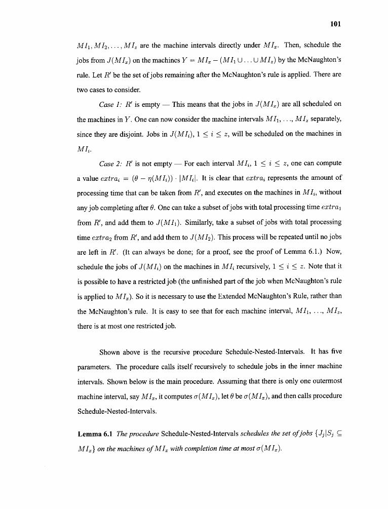
101

MI1, M 12 , , MIz are the machine intervals directly under MIT. Then, schedule the

jobs from J(MIx ) on the machines Y = UU. . . U MIz ) by the McNaughton's

rule. Let R' be the set of jobs remaining after the McNaughton's rule is applied. There are

two cases to consider.

Case 1: R' is empty — This means that the jobs in J(MIx ) are all scheduled on

the machines in Y. One can now consider the machine intervals MI 1 , . . M Iz separately,

since they are disjoint. Jobs in J(MIi ), 1 ≤ i ≤ z, will be scheduled on the machines in

M Ii.

Case 2: R' is not empty — For each interval MI i , 1 < i < z, one can compute

a value extrai = (0 — η(MIi)) • 1M It is clear that extrai represents the amount of

processing time that can be taken from R', and executes on the machines in MIi , without

any job completing after 0. One can take a subset of jobs with total processing time extra s

from R', and add them to J(MI1 ). Similarly, take a subset of jobs with total processing

time extra2 from R', and add them to J(MI2 ). This process will be repeated until no jobs

are left in R'. (It can always be done; for a proof, see the proof of Lemma 6.1.) Now,

schedule the jobs of J(MIi) on the machines in MI i recursively, 1 ≤ i ≤ z. Note that it

is possible to have a restricted job (the unfinished part of the job when McNaughton's rule

is applied to MIT). So it is necessary to use the Extended McNaughton's Rule, rather than

the McNaughton's rule. It is easy to see that for each machine interval, MI1, . . M

there is at most one restricted job.

Shown above is the recursive procedure Schedule-Nested-Intervals. It has five

parameters. The procedure calls itself recursively to schedule jobs in the inner machine

intervals. Shown below is the main procedure. Assuming that there is only one outermost

machine interval, say MIT , it computes σ ( MIx ) , let 0 be σ ( MIx ) , and then calls procedure

Schedule-Nested-Intervals.

Lemma 6.1 The procedure Schedule-Nested-Intervals schedules the set of jobs {Jj│Sj C

MIT } on the machines of M Ix with completion time at most σ(MI x ).

102

Proof The correctness of the lemma can be proved by induction on the level of MIx . If

the level of MIx is 1, the algorithm is essentially McNaughton's rule and Cmax = σ(MIx ).

Assuming that the lemma is true if the level of MIX is h, the goal is to prove

that it is also true if the level of MIx is h + 1. If the level of MIX is h + 1, then for

each machine interval MIi , 1 ≤ i ≤ z, directly under MIx , the total processing time

of the extra jobs assigned to it is at most (σ (MIx ) — n(MIi )) • IMIi l. So, σ(MIi) is

at most σ(MIx). By the inductive hypothesis, one can obtain a feasible schedule with

completion time at most σ(MIx ) for each MIi , 1 < i < z. The schedule for the machines

103

in Y = MIx — (MI1 U ... U MIS ) is obtained by the Extended McNaughton's Rule. So

its completion time is at most σ (MIx ) as well.

It remains to be shown that no job (or job part) left after assigning the jobs of R'

to MI1 , . . MIi . Suppose not, then the total processing time on each machine of MIx

is exactly σ(MIx ). So, the total processing time of the jobs of Pj Sj C MIx } is strictly

greater than σ(MIx ) • I MIx│ . This contradicts the definition of σ(MIx ). ❑

From Lemma 6.1, one can obtain a feasible schedule with Cmax = σ ( MIx ) , by

using the procedure Schedule-Nested-Intervals. It is optimal because σ (MIx ) is a trivial

lower bound of any feasible schedule. The running time of the Extended McNaughton's

Rule is linear with respect to the number of jobs scheduled. As mentioned before, there is at

most one restricted job for each machine interval. So the number of restricted jobs is 0(m).

Only the restricted jobs will be considered in different machine intervals. Therefore, the

running time of the algorithm is 0(m + n). 1 Since it is reasonable to assume that n > m,

the running time is 0(n).

Theorem 6.2 The procedure Schedule-Nested-Intervals produces an optimal schedule

with running time 0(n).

6.3 A Maximal Algorithm

Hong and Leung [Hong and Leung 1992] give a maximal algorithm for the problem P

pmtn I Cmax ; their algorithm can be extended to an online algorithm for the problem

P I pmtn, rj I Cmax as well. It is shown in this section that their algorithm can be adapted

to produce a maximal schedule for this problem as well.

6.3.1 Hong and Leung's Algorithm

One may assume that the processing time of the jobs are in nonincreasing order; i.e., p i ≥

P2 ≥ MI . Hong and Leung's algorithm works as follows.

'One can assume that the intervals have been organized as an interval tree so each directly nestedmachine interval can be retrieved in constant time.

104

otherwise, it is called the short job. It is clear that each long job is scheduled exclusively

on a single machine by Hong and Leung's algorithm, while the short jobs are scheduled by

McNaughton's rule. For any machine, let the total processing time of the jobs assigned to

the machine be the length of the machine. The machine with the shortest length is called

the shortest machine.

Lemma 6.3 Given a schedule S for the m machines, let l(Mi ) be the length of machine

A and J(Mi ) be the set of jobs assigned to machine A. Suppose

Let S' be a new schedule produced by Hong and Leung 's algorithm on the same set of jobs,

but without the constraint (3); i.e., any job in J(M i ), k + 1 < i < m, can be scheduled on

any machines. Suppose the length of the shortest machine in S' is c, and c > l(Mm ) . Then,

there is a feasible schedule S" such that

1. there is no idle time on any machine before time instant c.

2. any job not finished by the time instant c is scheduled continuously from time 0 until

it completes.

105

Proof Schedule 5" is obtained from S' as follows. In S', divide all jobs into two subsets

G and H: G contains all jobs (or job parts) executed after time c and H contains all jobs

(or job parts) executed before time c.

To obtain schedule S", one can first reschedule the jobs in H by using the procedure

Schedule-Nested-Intervals as described in Section 6.2. It is easy to see that 0 = c. So all

jobs can be finished by time c. Since there is no idle time before c in S', there is no idle

time before time c in 5" as well.

For each job of G, it will be scheduled on one machine, starting from time c. There

are at most m such jobs. For each job in G, there is a part with processing time exactly c in

H. So this job part must be scheduled continuously from time 0 until c. This implies that

the job must be scheduled continuously from time 0 until it completes in S". ❑

6.3.2 Maximal Algorithm

The algorithm works from the innermost interval to the outermost interval. For the

innermost interval, jobs are scheduled by Hong and Leung's algorithm. The algorithm is

presented recursively. Suppose currently machine interval MIx is processed, under which

are the machine intervals MI1 , . . ., MIz . First, schedule the jobs in AM Ix ) on the

machines Y = MIx — (MI1U...UMIz) by Hong and Leung's algorithm. There are two

cases to consider.

Case 1: The length of the shortest machine in Y is less than or equal to the length

of the shortest machine in MI 1 UU. . . U MI,. In this case, the interval MIx is done, and one

can proceed to schedule its outer interval.

Case 2: The length of the shortest machine in Y is greater than the length of the

shortest machine in MI1 UU. . . U MIX . In this case, more work needs to be done as follows.

One may assume that the machines in MI 1 U . . . U MI, is relabeled in ascending order of

their lengths; i.e., l(M1 ) < l(M2) ≤ ... < l(Mg ). Now find the largest index g' such that

Lemma 6.3 can be applied on the machines in YU{M 1 , M2, ... , Mg'}. (Recall that to apply

Lemma 6.3, one thing that must be sure is that after applying Hong and Leung's algorithm,

the length of shortest machine must be greater than or equal to l(Mg')). g' can be obtained

106

by iteratively adding one machine from {M 1 , , Mg } until the first time a machine g' + 1

such that Lemma 6.3 can not be applied to the set of machines {M1, M25 • • • , Mg'+1 } is

encountered. The jobs on the machines Y U {M 1 , M2 , . , Mg'} is then rescheduled by

the method as described in Lemma 6.3. Suppose c is the length of the shortest machine in

Y U M2, , Mg'}. It is clear that c ≤ /(M9 ' +1 ) ≤ . . . ≤ /(Mg ).

Figure 1 illustrates the maximal algorithm when applied to the set of jobs in

Example 1. Figure 1(a) shows the schedule after the maximal algorithm schedules the two

innermost intervals. Figure 1(b) shows the schedule after the maximal algorithm schedules

the jobs of J(MIi ) on the machines in Y (M1 , M2 and M3 ). Figure 1(c) shows the schedule

after the maximal algorithm merges the machines in Y with M5 and M6. Figure 1(d) shows

the schedule after the maximal algorithm merges the machines M3, M5 and M6 with the

machines M8, M9 and M10 . Figure l(e) shows the final schedule.

Figure 6.1 An example illustrating the maximal algorithm. Figure 6.1(a) shows theschedule of the innermost intervals. Figure 6.1(b) shows the schedule of the outermostinterval on the machines in Y. Figure 6.1(c) and Figure 6.l(d) shows the iterations to findthe set of machines to be merged. Figure 6.l(e) shows the final schedule.

Shown below is the procedure Maximal-Schedule-One-Interval. It schedules the

jobs in one machine interval only, namely, MIT . The main procedure will repeatedly call

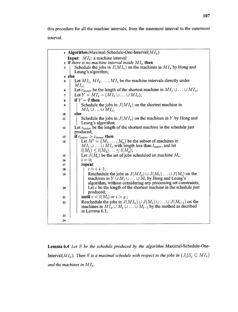
107

this procedure for all the machine intervals, from the innermost interval to the outermost

interval.

Lemma 6.4 Let S be the schedule produced by the algorithm

Maximal-Schedule-One-Interval(MIx).Then S is a maximal schedule with respect to the jobs in C M Ix}

and the machines in M Ix.

108

Proof: The lemma can be proven by induction on the level of M Ix . If the level of M Ix is

1, then the algorithm is the same as Hong and Leung's algorithm, and hence the schedule

it produces is maximal.

Assume the lemma is true if the level of M Ix is less than or equal to h. One can

prove that it is also true when the level of M Ix is h+ 1. Suppose S is the schedule produced

by the algorithm and S is not maximal. Then there is a schedule 5* and a time instant t such

that the amount of work done by all machines in the time interval [0, t] is strictly greater

than that done by S. Let c be the length of the shortest machine in the schedule S. One

may assume that t > c. There are two cases to consider.

Case 1: Before time t, S* executes more of the jobs from J(MIx ) than S. In this

case, by Lemma 6.3, the jobs from J(MIx ) is either finished before time c or it is scheduled

continuously from time 0 until it finishes. Therefore, S* cannot execute more of the jobs

from J(M Ix ) than S.

Case 2: Before time t, S* executes more of the jobs in J(MIi ), 1 < i < z, than S.

In this case, it is clear that the jobs in J(MIi ) can only be scheduled on the machines in the

machine interval MIi . Denote the schedule on the machines of MI i , before rescheduling,

by S. By the inductive hypothesis, S is maximal with respect to all the jobs that can be

scheduled on the machines in MIi . For any machine Me E MIi , if Mi ' is not rescheduled,

then before time t, the total amount of processing done on Mi ' by S is the same as that

of if Mir is rescheduled, it is clear that all jobs scheduled by S on machine M i ' are

also finished by S before time c. So before time t, S* cannot execute more of the jobs in

J(MIi ), 1 < i < z, than S.

Summarize the discussion above, S is a maximal schedule. ❑

109

The fist step of this algorithm is running Hong and Leung's algorithm on the

machines in Y; the running time is O(│J(MIx ) I log 1 J(M Ix). Next, one needs to find

the first g' machines to fulfill the requirment of Lemma 6.3. The running time of Hong and

Leung's algorithm is 0(n log n) for n jobs. But it is known that only the jobs in J MIx)

can be long jobs, and one only needs to compute the length of the shortest machine instead

of schedule all the jobs. So the running time of each try is O(│J(MIx)│). If binary search

instead of searching g' sequentially is used, the running time will be O(│J(M Ix )1 log m).

Finally, one needs 0(n) time to reschedule all the machines involved. The total running

time is clearly 0 (n +│J(MIx ) (log m + log │J(MIx )│)).

The machine intervals are scheduled from the innermost one to the outermost one.

When the outermost interval is reached, one will obtain a maximal schedule. Since there

are at most 0(m) intervals, and for each interval, the running time for M Ix is 0(n +

J(M Ix )I (log m + log I J(MIx │)), the total running time is 0(mn +n(log m + log n)). It

becomes O(mn + n log n) if assuming n is greater than m.

Theorem 6.5 For nested intervals, the algorithm Maximal-Schedule produces a maximal

schedule in time O(mn + n log n).

6.4 Different Release Times

In this section, it is assumed that the jobs have different release times. Let r0 < r 1 <

. . . < rk- 1 be the k distinct release times. Without loss of generality, one may assume that

r0 = 0. An upper bound for the optimal makespan is U = rk-1 + Σnj=1pj and an obvious

lower bound is L = rk-1. One can conduct a binary search in the interval [L, U], searching

for the optimal makespan C*. For each value C obtained in the binary search, one can test

if there is a feasible schedule with makespan C.

First, divide the time span into k segments: TS0 = [r0, ri], TS1 = [r1, r2], • •

TSk- 1 = [rk-1, C]. For each segment TSj , 0 ≤ j ≤ k — 1, use l(TSj ) to denote the

length of the segement. In the next subsection, a network flow approach is given to solve

110

the nested processing set case, followed by a more efficient algorithm for the inclusive

processing set case.

6.4.1 Nested Processing Set

For the nested processing set case, one can construct a network with nodes and arcs as

follows. it will be shown later that there is a feasible schedule with makespan C if and only

• For each machine A, 1 < i < m, and each time segment TS; , 0 ≤ j ≤ k — 1, anode Mi, j is created. The node is called a machine-segment node.

• For each job Jj , 1 ≤ j ≤ n, nodes Jj,t, Jj,t+1, • • Jj , k-1 are created, where therelease time of Jj is rt . Call these nodes the job-segment nodes.

• For each job J, , 1 < j < n, a job node Jj is created. Finally, a source node S and asink node T are added.

• For each job node Jj , an arc is added from S to Jj with capacity pj .

• For each job node J.; and each job-segment node Jj , q , t ≤ q ≤ k — 1, an arc is addedfrom Jj to Jj , q with capacity l(TSq ).

• For each job-segment node Jj ,q and each machine-segment node Mi , q , if Jj can bescheduled on machine A, then an arc is added from Jj ,q to Mi , q with capacity1(T S q )

• For each machine-segment node Mi , q , an arc is added from Mi , q to the sink T withcapacity l(T SO.

Figure 6.2 shows the picture for three jobs and two machines. There are three

release times: r0 , r1 and r2 . Job 1 is released at r0 , job 2 is released at r1 and job 3 is

released at r2 . Job 1 can be scheduled on machines M 1 and M2, while jobs 2 and 3 can

only be scheduled on M2.

Lemma 6.6 There is a _feasible schedule with makespan C if and only if the solution of

111

Figure 6.2 The reduction to maxflow problem.

Proof: A known fact is introduced to facilitate the proving Lemma 6.6, ; see

Gonzalez and Sahni [Gonzalez and Sahni 1976].

Lemma 6.7 Let T be am x n matrix such that T(i, j) denotes the total processing time of

there is a feasible preemptive schedule with makespan at most C. Moreover the schedule

can be found in time 0(m 2 n2 ).

Given a feasible schedule with makespan at most C, it is easy to see that the max-

Given the max-flow of the network constructed above, if the flow on the arc

Mi ,q) is x, then one can schedule job Jj on machine i in the time segment TSq for x

time units. It is easy to see that for any time segment TSq : (l) for each job Jj , the total

amount of Jj scheduled in TSq will never exceed /(TSq ), and (2) for each machine-segment

Mi , q , the total processing time assigned to s Mi , q, will never exceed l(TSq). Because of

Lemma 6.7, there is a feasible schedule in the time segment TSq .

There are 0( (m + n)k) nodes and 0 (mnk) edges in the network. One may assume

that n > m. Using the max-flow algorithm of Goldberg and Tarjan [Goldberg and Tarjan

112

One needs to construct the schedule segment by segment. For each time segment, One

needs to solve a stochastic matrix with running time O(m 2 n2 ) .) Therefore, the total time

for solving all intervals is O (m2 n2k).

Theorem 6.8 For the nested processing set case, an optimal schedule can be obtained in

6.4.2 Inclusive Processing Set

In this section, a more efficient algorithm is given for the inclusive processing set case. For

convenience of presentation, let rk = C*. First, do some preprocessing on the jobs: for

any job J1 released at time ri , if pl is greater than ri+1 — ri , then cut it into two pieces: a

job Ji' released at ri with processing time ri+1 — ri , and a job Jr released at time ri+1 with

processing time pl — (ri+1—ri). If the processing time of Jr is still greater than ri+2 —ri+1 , it

is cut once again into two pieces, and so on. After the preprocessing step, one may assume

that for any job released at time ri , its processing time is less than or equal to ri+1 — ri . An

array T(l, i), 1 < l < n and 0 < i ≤ k —1 is used to store the processing time of job l in the

time segment TSi . Clearly, T(l, i) = 0 if the release time of job l is greater than ri.When

constructing the optimal schedule, T(l, i) will be updated so that it reflects the amount of

processing of job I done in the time segment TSi in the optimal schedule. Once T(l, i) is

updated, the optimal schedule can be obtained by McNaughton's rule segment by segment,

and within each segment the jobs are scheduled from the outermost machine interval to the

innermost one.

Assume there are z machine intervals in the job set: MI1 D MI2 D D MIS . For

each machine interval MIj , 1 < j < z —1, let Yj denote the machines in —MIj+1, and

let Y., denote all the machines in MIz . An array IDLE(j,i),1< j ≤ z and 0 ≤ i ≤ k —1

is used to store the total idle times on the machines in Y3 during the time segment TSi.

From now on, assume that for every time segment, there are exactly z machine intervals.

The symbol J(MIj, i) is used to denote the set of jobs with machine interval MI; released

113

at time ri . Clearly, J(MIj , i) = 0 if there is no job with machine interval MI; released at

time ri .

In the next subsection, a test will be given to see if there is a feasible schedule

with makespan C. In the following subsection, an algorithm will be described to obtain an

optimal schedule once the optimal makespan C* is determined.

Feasibility Test The algorithm works backwards in time. The time segment TSk-1 =

[rk-1,rk ] can easily be determined. The jobs are scheduled by McNaughton's rule, starting

with the jobs in the outermost interval and ending with the jobs in the innermost interval.

If some jobs cannot be feasibly scheduled, one can declare that it is impossible to have a

schedule with makespan C. Otherwise, IDLE(j,k — 1) is computed for all 1 ≤ j ≤ z.

Let βj = IDLE(j, k — 1) for all 1 ≤ j ≤ z.

Suppose it have been determined that the jobs in the time segment [ri+1 , ri+2 ] can

be feasibly scheduled. Now consider the jobs released at time ri . the jobs are considered

from the outermost interval to the innermost interval. For each MIS , 1 < j < z, let extras

be the total idle times on the machines in Y (i.e., the total idle times in the interval [ri , ri+1 ]

plus the total idle times in the interval [ri+1 , rd, minus the total processing times of the jobs

in J(MIj , i)). If extras < 0, then some jobs in this machine interval have to be scheduled

on some other machines of an inner interval.

After extras is computed, the following procedure (Algorithm Compute-Idle-and-

Test-Feasibility) can be used to compute the amount of processing times needed to be

moved between any pair of Y's. The variable move(p, q) is used to store the amount

of processing times needed to be moved from the machines in Yp to the machines in Yq .

extras is also updated for 1 < j < z. Finally, let (3.; = extras for 1 ≤ j ≤ z.

The running time of algorithm Compute-Idle-and-Test-Feasibility for one time

segment is 0(m + ni ), where ni is the number of jobs released at ri . The for-loop in

Steps 2 to 3 takes 0(m + n i ) time. The for-loop in Steps 5 to 16 takes 0(m) time because

in each iteration, either the value of p is increased, or the value of q is increased, and the

algorithm will terminate when either p or q reaches z. The for-loop in Steps 17 to 18 takes

114

0(m) time. Thus, the overall running time for testing k time segments is 0 ((m n)k).

Since one may assume that n > m, the running time becomes O(nk). To find the optimal

The above algorithm determines if there is enough room to schedule the jobs

released at ri . But there is one issue that needs to be resolved. It is possible that a job

released at ri is the same job as the jobs released at ri+1, due to the preprocessing

step. Therefore, the jobs released at ri must be scheduled carefully so that there is no

overlap with the same jobs in subsequent time segments. Fortunately, it can be shown

that the jobs can indeed be feasibly scheduled if the jobs released at ri pass the test of

Algorithm Compute-Idle-and-Test-Feasibility. In the next subsection, an algorithm will be

given to construct an optimal schedule.

Obtaining An Optimal Schedule As was mentioned in Section 6.4.2, to obtain an

optimal schedule, T(l, i) needs to be computed which stores the amount of processing

of job l done in the time segment TSi in an optimal schedule. Initially, T(l, i) is the

processing time of job l in the time segment TSi . T(l, i) is computed backwards in time,

starting with the time segment TSk-1 . T(l, k — 1) is exactly the initial value. The jobs

115

are then scheduled in the time segment TSk- 1 by McNaughton's rule, starting with the

jobs in the outermost interval and ending with the jobs in the innermost interval. From the

schedule, set IDLE(j, k — 1), 1 < j < z to be the total idle times on the machines in Y.;

during the time segment TSk-1 . Let αj = IDLE(j, k — 1) for all 1 ≤ j ≤ k — 1.

Suppose T(l, i + 1) has been computed for the jobs in the time segment TSi+1.

Now consider the jobs released at time ri . For each machine interval MIS , let αj =

Σxk=i-1+1 IDLE(j, x); i.e., αj is the total idle times on the machines of Yj after time

ri+1 . Then algorithm Compute-Idle-and-Test-Feasibility is invoked to test feasibility for

this time segment. Algorithm Compute-Idle-and-Test-Feasibility will compute extra.' and

move(p, q), in addition to testing feasibility; see the algorithm in Section 6.4.2

After the Algorithm Compute-Idle-and-Test-Feasibility is called, if extras ≥ αj,

then there is no need to fill any job in the idle times in IDLE(j, x), i +1 ≤ x ≤ k — 1.

The jobs in J(MIj , i) will be scheduled exclusively on the machines of Y.; in the time

segment [ri , ri+1 ]. On the other hand, if extras < αj, then besides scheduling all the

machines of Yj in the time segment [ri , ri+1 ], one needs to fill in an amount of processing

time equal to fin.; = αj — extras in the idle times in I D LE(j, x), i 1 ≤ x ≤ k — 1. Let

fill.; = max{αj — extras , 0} for all 1 < j < z.

If f illy = 0 for each machine interval MIS , then all the jobs released at time ri will

be scheduled in the time segment T Si . Thus, T(l, i) will be the same as the initial value.

McNaughton's rule can be used to construct a schedule in this segment. From the schedule,

I DLE(j,i) is updated for all 1 ≤ j ≤ z.

If fillj > 0 for some machine interval then it is necessary to fill some jobs

released at time ri in the idle times in IDLE(j, x), i + 1 < x < k — 1. It is possible

that a job released at ri is the same job as the jobs released at ri+1 , , rk—1, due to the

preprocessing step. Therefore, the jobs released at ri must be scheduled carefully so as

to avoid any overlap with the same job in subsequent time segments. In the following,

a method to schedule these jobs will be described. The basic idea is that first jobs with

total processing times equal to fillj will be scheduled in the idle times in IDLE(j, x),

i + 1 ≤ x ≤ k — 1. After this step is finished for all the machine intervals, the remaining

116

jobs will be scheduled in the time segment TSi by McNaughton's rule. Finally, IDLE(j, i)

is updated for all 1 ≤ j ≤ z.

Suppose pil l > 0. Then the jobs of J(MI1 , i) is scheduled with total processing

times equal to fill s in the idle times in IDLE(1, x), i + 1 ≤ x ≤ k — 1, on the machines

of Y1 . The jobs are scheduled in the following manner. For any job l E i), this job

is tried to schedule in the idle times in IDLE(1, i + 1) if IDLE(1, i + 1) > 0. One can

schedule job l for an amount equal to min{fill1, IDLE(1, i + 1), T(l, i), ri+2 — ri+1—

T(l, i + 1)} in the time segment TSi+1. Then IDLE(1,i +1),T(l, i) and T(l, i + 1)

are updated. If job l is completely scheduled and IDLE(1, i + 1) is still greater than 0,

another job of J(MI1 , i) is tried to scheduled in the idle times in IDLE(1, i + 1) using the

same method. If job l still has some processing time not scheduled, it is tried to schedule

in IDLE(1, i + 2) and so on. It will be shown later in Lemma 6.9 that one can always

schedule the jobs of J(MI1 , i) with total processing times equal to fill]. in the idle times

in IDLE(1, x), i +1 < x < k — 1, without producing any overlap.

Now, consider the next machine interval Y with finj > 0 and j > 1. First find

the maximum machine interval index p such that no processing time need to be moved

from Ya to Yb for any 1 < a < p — 1 and p < b < j; i.e., move(a, b) = 0 for all

1 < a < p — 1 and p < b < j. Then, for each pair of indexes c and d such that p ri+2

c < d — 1 < j — 1 and move(c, d) > 0, the value move(c, d) is added to each item

move(c, c + 1), move(c + 1, c + 2) , . . . , and move(d — 1, d). Finally, set move(c, d) to be

0.

Then, from g = p to j — 1, all jobs of J(MIg , i) will be tried to fill in a total amount

up to at most min{fillj , move(g, g + 1), move(g + 1, g + 2), . . . , move(j — 1, j)} in the

idle times in IDLE(j, x), i + 1 < x < k — 1, on the machines of Y. Each job is filled

in exactly the same manner as in the idle times in IDLE(1, x), i + 1 ≤ x ≤ k — 1. Let

pg be the total processing times among all jobs of J(MIg , i) that is filled in. The sequence

move(g, g + 1), move(g + 1, g + 2), , move(j — 1, j) will be updated by reducing p9

from them, and the array T(.,.) and IDLE(j, x), i + 1 < x < k — 1 are updated. This

procedure will be stopped when either fillj = 0 or all jobs of J(MIp ,i), J(MIp+1, i ),..., . .

117

and J(MIj- 1 , i) have been tried. In the latter case, all jobs of J(MIj , i) will be tried to

fill in an amount equal to filly in the idle times in IDLE(j, x), i +1 ≤ x ≤ k — 1, on

the machines of Yj , and the array T(.,.) and IDLE(j,x) are updated. (Again, the jobs are

filled in exactly the same manner as in the idle times in IDLE(1, x), i +1 ≤ x ≤ k — 1.)

It will be shown later in Lemma 6.9 that one can always schedule jobs of J(MIj , i) with

total processing times fillj in the idle times in IDLE(j,x),i +1 ≤ x ≤ k —1, without

producing any overlap. After all the machine intervals yj with fillj > 0 are considered by

the above procedure, every machine interval Y must have fillj = 0. Then the remaining

jobs T(l, i), 1 < l < n are scheduled, in the time segment T Si by McNaughton's rule.

From the schedule, IDLE(j, i), 1 < j < z is updated. The process described above is

shown in the algorithm Schedule-Inclusive-Intervals-with-Release-Time.

The procedure is repeated for all the time segments. After all the time segments are

finished, T(l, i) is computed for any job l and any 0 < i < k —1. Then a feasible schedule

can be obtained by McNaughton's rule, segment by segment.

Lemma 6.9 Suppose the jobs released at time ri passed the test of Algorithm Compute-

Idle-and-Test-Feasibility. For each machine interval Y , one can fill in exactly fill j amount

of processing time in the idle times in I DLE(j, x) for i + 1 ≤ x ≤ k — 1 by algorithm

Schedule-Inclusive-Intervals-with-Release-Time, without any overlap.

Proof: First, it is easy to see that no overlap can be produced by algorithm Schedule-

Inclusive-Intervals-with-Release-Time and for each machine interval Y , no more than f ill

amount of processing time is filled in the idle times in IDLE(j, x) for i + 1 ≤ x ≤ k —1.

Now one can prove that for each machine interval one can always fill in at least fillj

amount of processing time in the idle times in IDLE( j,x) for i + 1 ≤ x ≤ k —1. For

any set J of jobs, let p(J) denote the total processing times of all the jobs in J. It will be

proven, by induction on j, the following claim.

118

Claim 6.10 For any machine interval 1 < j < z, with extras < after algorithm

Compute-Idle-and-Test-Feasibility is called, the following equation always holds:

Recall that αj is the total idle times in IDLE(j, x) tor z + 1 ≤ x ≤ — 1 before

algorithm Compute-Idle-and-Test-Feasibility is called in this iteration, and extras is the

total idle times in I D LE (j , x) for i ≤ x ≤ k — 1 after algorithm Compute-Idle-and-Test-

Feasibility is called in this iteration. So the claim means that after algorithm Compute-Idle-

and-Test-Feasibility is called, for any machine interval Y in which at least I Yj * (ri+1 — ri)

of processing times can be filled, the total processing times of J(MIj , i) plus the total

processing times that needs to be moved to Y minus the total processing times that needs

to be moved out of Y is exactly equal to the total idle times in Y in the time segment TSi

plus f ill j .

The claim can be proven by induction on j. For the base case j = 1, if f ill s = 0,

the claim clearly holds. On the other hand, if f ill s > 0, then

It can be shown that one can always schedule jobs of J(MIi , i) with total processing times

fill ]. in the idle times in IDLE(1, x) for i + 1 < x < k-1 on the machines of Y1 . Suppose

not. Then there must be a time segment b, i 1 ≤ b < k — 1), such that some idle time of

IDLE(1, b) can not be filled. Since p(J(MI1,i))> Y1 * (ri+1 ri ), then at least 1Y1 1 jobs

are in J(MI1 , i). Since all these jobs can not be filled in IDLE(1, b), they must have been

scheduled in the time segment TSb for a duration equal to rb+1 — rb. But this means that

there is no idle time on the machines of Y1 , contradicting the fact that IDLE(1,b)> 0.

After f ill, amount of processing times is filled in the idle times in IDLE(1,x),

119

Assume that the claim holds for the first j — 1 machine intervals. Next one can

prove that it also holds for the j-th interval. If fill ; = 0, the claim obviously holds. If

p be the total processing time that is filled. the sequence move(g, g + 1), move(g +

1, g + 2), , move[j — 1][j] is updated by reducing p from each of them. Furthermore,

fin.; is also updated in the course of scheduling the jobs. Finally, J(MIg , i) is updated

by removing all the scheduled jobs or parts of the jobs. Since both move (j — 1, j)

and fillj are reduced by p and other items are not changed, the following equation still

Similarly, since both move(g, g + 1) and p(J(M i)) are educed by p and other items

are not changed, the following equation still holds: p(J(M i)) + move(g — 1, g) —

change in other machine intervals, so all the equations still hold.

120

The procedure is stopped when either fillj = 0 or all jobs of J(MIp , i),

J(MIp+1 , i), . . ., and J(MIj-1 , i) have been tried. If, after all jobs of J(MIp ,i),

. . ., and J(MIj-1, i) have been tried, filly is still greater than 0, then all

jobs of J(MIj , i) are tried to schedule fill.; amount of processing time in the idle times in

IDLE(j, x) for i + 1 < x < k — 1 on the machines of Y , and J(MIj , i) is updated by

removing all the scheduled jobs or parts of the jobs. Since both p(J(M j , i)) and fill; are

reduced by the same amount and the other items are not changed, the following equation

Now it can be shown that after all the jobs of J(MIj , i) have been tried, fillj must

be 0. Suppose not. Let w be the last machine index such that move(w, w + 1) = 0. That is,

from w+1 on, each time one try to fill min{ f illy , move(x, x+1), . , move(j —1, j)}, x >

w, of processing time in the idle times in I D LE(j, x), i +1 < x < k — 1, on the machines

of Y, it is only possible to fill only (5 < min{ fillj ,move(x,x + 1), . , move(j — 1, j)}

of processing time in the idle times in IDLE(j, x), i 1 < x < k — 1, on the machines

of Yj . That means all the jobs in J(MIx , i), w + 1 < x < j are tried, to fill in the idle

times in I D LE(j, x), i + 1 ≤ x ≤ k — 1. Since fill.; > 0, there must be a time segment

b, i + 1 < b < k — 1), such that some idle time in IDLE(j, b) can not be filled. Since for

each w + 1 < u < j, then

then,

121

and

Notice that fillu = 0 for all w + 1 < u < j — 1. Thus, p(J(MIw+1,i)) +

P(J(MIw+2,i))+ • • ,+ P(J(MIj,i)) (Yw+1 + Yw+2+ • • • + (ri+1 — ri) + filly .

Since each of these jobs has length at most (ri+1 — ri), there must be at least

+ lYw+2 + • • • + MI jobs in J(MI w+1, i), J(MIw+2, i), ..., and J(MIj , i). Since

all these jobs can not be filled in the idle times in IDLE(j, b), these jobs must have been

scheduled in the time segment TSb for a duration equal to (rb+1 — rb). Therefore, there

should be no idle time in time segment TSb on the machines of contradicting the fact

that IDLE(j,b)> 0.

So, for machine interval Yj , the claim still holds and exactly fillj of processing

time can be filled in the idle times in IDLE(j, x), i + I< x < k — 1, on the machines of

Yj •

Algorithm 6.1 constructs the schedule for one time segment. Steps 1 to 6 take

0(n + m) times. Step 9 takes 0(m) time for each machine interval MIS . Since there are

0(m) machine intervals, Step 9 takes a total of 0(m 2 ) time. Steps 10 to 13 take 0 (m3 )

time since there are 0(m2 ) pairs of c and d. Steps 15 to 22 take 0 (mnk) time. Therefore,

the total time needed for one time segment is O(mnk +m 3 ). Hence the total time for k time

segment is 0(mnk2 + m3k). After the array T(•,.) is updated, one can obtain a schedule

by McNaughton's rule which takes O(nk) time.

Theorem 6.11 For the inclusive processing set case, one can obtain an optimal schedule

in time O(nk log P + mnk 2 + m3 k).

122

6.5 Conclusion

In this paper first an efficient algorithm for constructing a minimal length preemptive

schedule for nested processing set (and hence inclusive processing set) restrictions is given.

An efficient algorithm for generating maximal schedules is also given. When jobs have

different release times, a network flow approach can be used to construct an optimal

schedule. A more efficient algorithm is given for the inclusive processing set restriction.

The network flow approach also works for arbitrary processing set restriction. For future

research, it will be interesting to see if there are more efficient algorithms than the ones

presented in this paper.

Online scheduling algorithm is considered as well. Since there is no optimal online

algorithm, the best one can hope for is an approximation algorithm. In this regard, the

maximal algorithm presented in Section 6.3 have been considered as an approximation

algorithm. Whenever new jobs arrive, the unfinished portions of the jobs along with the

new jobs are reschedule. What is the competitive ratio of this algorithm? It is possible

to show that the competitive ratio lies between 3/2 and 2. For future research, it will be

interesting to determine the exact value of the competitive ratio of this algorithm.

123

Figure 6.3 Fast algorithm for inclusive restrictions.

CHAPTER 7

CONCLUSIONS

This dissertation studied combinatorial optimization problems arising from two areas:

radio network and scheduling. The main focus was to design efficient algorithms for some

combinatorial problems.

7.1 Communication in Random Geometric Radio Networks

The first model studied in this dissertation is a uni-disk model, the main model for wireless

communication. It has been shown in this dissertation that when network is sparse: (l)A

simple randomized algorithm can be used to do gossiping in 0(D) steps, without any

geometric position knowledge. (2)A deterministic algorithm can be used to do gossiping in

0(D) steps if every node know its own geometric position. (3)A deterministic algorithm

can be used to do gossiping in 0(D) steps if the distance or angle between two nodes can

be determined by checking the incoming signal. Since D is a trivial lower bound for doing

any global communication in the network, all these algorithms are asymptoticly optimal.

These results will appear in [Czumaj and Wang 2007b].

The second model studied in this dissertation is the random line-of-sight radio

network. In this dissertation, it has been shown when network is sparse: (1)A deterministic

algorithm can be used to do gossiping in 0(D) steps, if every node knows its own geometric

position. (2)A deterministic algorithm can be used to do broadcasting in 0(D) steps

without having any geometric knowledge. (3)A randomized algorithm can be used to do

gossiping in 0(D) steps without having any geometric knowledge. Again, the running

time of all these algorithms is asymptoticly optimal. These results have been published in

[Czumaj and Wang 2007a].

There are several questions that have not been answered. In this dissertation, in

both models, the networks are assumed to be sparse. When network becomes dense, the

124

125

running time of these algorithms is significantly increased. It will be interesting to design

faster algorithms for dense networks.

7.2 Scheduling Problems

In scheduling area, the first model studied in this dissertation is the online scheduling of

equal processing time task systems. It has been shown that Algorithm Delay-A has an

asymptotic competitive ratio of 3/2 for P pj = p, intreei released at time ri Cmax, and

an asymptotic competitive ratio of 1 for P pj = p, outtreei released at time r i Cmax •

Furthermore, it is shown that Algorithm Delay-B has an asymptotic competitive ratio of 1

for P2 pj = p, preci released at time r i Cmax . All this results have been submitted for

review [Huo et al. 2007b].

There are several open problems for this model. For the problem P I pj =

p, preci released at time ri Cmax , the asymptotic competitive ratio of Algorithm Delay-B

has not been determined. On the other hand, it is known that the ratio is at least 2 —

since Lam and Sethi [Lam and Sethi 1977] have shown that Coffman-Graham algorithm is

a (2 — !)-approximation algorithm for P pj = 1, prec Cmax . For future research, it

will be interesting to determine this value. Furthermore, it will be interesting to see if there

are other classes of precedence constraints and processing times that yield an asymptotic

competitive ratio less than 2. Since for P pmtn, intree Cmax, Muntz-Coffman

algorithm gives an optimal solution, one can consider an online version of Muntz-Coffman

algorithm for P I pmtn, intree i released at time ri I Cmax . It will be interesting to know

the competitive ratio of this algorithm.

The second model studied in this dissertation is a scheduling model integrated

production and delivery. Each job is supposed to be completed within a specified time

window and the time windows are disjoint. Three kinds of profits are considered: (l)

arbitrary profit, (2) equal profit, and (3) profit proportional to its processing time. In the

first case, a pseudo-polynomial time algorithm is given to find an optimal schedule for a

single machine. Based on the pseudo-polynomial time algorithm, A FPTAS with running

time 0( 72, ) is developed. In the second case, an 0(n log n)-time algorithm is given to

126

find an optimal schedule for a single machine. In the third case, an improved FPTAS is

given with running time 0( "n4 ). All algorithms can be extended to parallel and identical

machines with a certain degradation of performance bounds. For the equal profit case, a

7/5-approximation for the special case where there is a single time frame and m ≥ 2 identical

and parallel machines is given. All these results have been submitted for review [Huo et al.

2007a].

The model can be extended in several direction. For example, a job not scheduled

incurs a small penalty; the delivery capacity is limited (at most c jobs can be delivered

every time); or the time windows are not disjoint.

The third model studied in this dissertation is preemptive scheduling with nested

and inclusive processing set restrictions. Four algorithms are given in this dissertation:

(1)An efficient algorithm for constructing a minimal length preemptive schedule for nested

processing set (and hence inclusive processing set) restrictions. (2)An efficient algorithm

for generating maximal schedules. (3) A network flow approach to construct an optimal

schedule when jobs have different release times. (4)A more efficient algorithm for the

inclusive processing set restriction when jobs have different release times. All these results

have been submitted for review [Huo et al. 2007c].

For future research, it will be interesting to see if there are more efficient algorithms

than the ones presented in this paper. Online scheduling algorithms are another interesting

topic. Since there is no optimal online algorithm, the best one can hope for is an

approximation algorithm. Especially, can the maximal algorithm presented in Chapter 6

be adapted to produce good competitive ratio?

REFERENCES

ALoN, N., BAR-NoY, A., LINIAL, N., AND PELEG, D. 1991. A lower bound for radiobroadcast. Journal of Computer and System Sciences 43, 2, 290-298.

BAR-NOY, A., GUHA, S., NAoR, J., AND SCHIEBER, B. 2001. Approximatingthe throughput of multiple machines in real-time scheduling. SIAM Journal onComputing 31, 2, 331-352.

BAR-YEHUDA, R., GoLDREICH, O., AND ITA1, A. 1992. On the time-complexity ofbroadcast in multi-hop radio networks: an exponential gap between determinism andrandomization. Journal of Computer and System Sciences 45, 1, 104-126.

BILGEN, B. AND OZKARAHAN, I. 2004. Strategic tactical and operationalproduction-distribution models: A review. International Journal of TechnologyManagement 28, 2, 151-171.

BOLLOBAS, B. 2001. Random graphs. Cambridge University Press, London, England.

BONIS,A. D.,GASIENIEC,L.,AND VACCARO,U. 2003. Generalized framework forselectors with applications in optimal group testing. In Proceedings of the 30thInternational Colloquium on Automata, Languages and Programming. 81-96.

CAPKUN, S., HAMDI, M., AND HUBAUX, J.-P. 2002. Gps-free positioning in mobile adhoc networks. Cluster Computing 5, 2, 157-167.

CHEN, B., PoTTS, C., AND WOEGINGER, G. 1998. A review of machinescheduling: Complexity, algorithms and approximability, Handbook of CombinatorialOptimization. Kluwer, Boston, Chapter 17, 21-169.

CHEN, Z.-L. 2004. Modeling in the E-Business Era, Handbook of Quantitative SupplyChain Analysis. Springer, Berlin, Chapter 17, 711-735.

CHEN, Z.-L. 2006. Integrated production and outbound distribution scheduling in a supplychain: Review and extensions, working paper.

CHLEBUS, B. 2001. Randomized communication in radio networks, Handbook onRandomized Computing. Kluwer Academic Publishers, Norwell, MA, USA,Chapter 11, 401-445.

CHLEBUS, B. S., GASIENIEC, L., GIBBoNS, A., PELC, A., AND RYTTER, W. 2002.Deterministic broadcasting in ad hoc radio networks. Distributed Computing 15, 1,27-38.

CHLEBUS, B. S., KoWALSKI, D. R., AND ROKICKI, M. A. 2006. Average-timecomplexity of gossiping in radio networks. In Proceedings of the 13th Colloquiumon Structural Information and Communication Complexity. 253-267.

CHRoBAK, M., GAS1ENIEC, L., AND RYTTER, W. 2002. Fast broadcasting and gossipingin radio networks. Journal of Algorithms 43, 2, 177-189.

127

128

CLEMENTI, A. E. F., MONTI, A., AND SILVESTRI, R. 2003. Distributed broadcast inradio networks of unknown topology. Theoretical Computer Science 302, l-3, 337-364.

COFFMAN, E. G., LEUNG, J. Y.-T., AND TING, D. W. 1978. Bin packing: Maximizingthe number of pieces packed. Acta Informatica 9, 263-271.

CZUMAJ, A. AND RYTTER, W. 2006. Broadcasting algorithms in radio networks withunknown topology. Journal of Algorithms 60, 2, 115-143.

CZUMAJ, A. AND WANG, X. 2007a. Communication problems in random line-of-sightad-hoc radio networks. In The 4th Symposium on Stochastic Algorithms, Foundations,and Applications. 70-81.

CZUMAJ, A. AND WANG, X. 2007b. Fast message dissemination in random geometricad-hoc radio networks. In The 18th International Symposium on Algorithms andComputation, to appear.

DESSMARK, A. AND PELC, A. 2007. Broadcasting in geometric radio networks. Journalof Discrete Algorithms 5, 1, 187-201.

DoHERTY, L., PISTER, K. S. J., AND GHAOUI, L. E. 2001. Convex optimizationmethods for sensor node position estimation. In Proceedings of the 20th Annual JointConference of the IEEE Computer and Communications Societies. 1655-1663.

ELSASSER, R. AND GASIENIEC, L. 2006. Radio communication in random graphs.Journal of Computer and System Sciences 72, 3, 490-506.

ERENGUC, S. S., SIMPSON, N. C., AND VAKHARIA, A. J. 1999. Integratedproduction/distribution planning in supply chains: An invited review. EuropeanJournal of Operational Research 115, 2, 219-236.

FRIEZE, A., KLEINBERG, J. M., RAVI, R., AND DEBANY, W. 2007. Line-of-sightnetworks. In Proceedings of the 18th ACM-SIAM Symposium on Discrete Algorithms.968-977.

GARC1A, J. M. AND LOZANO, S. 2005. Production and delivery scheduling problem withtime windows. Computers and Industrial Engineering 48, 4, 733-742.

GARCIA, J. M., LOZANO, S., AND CANCA, D. 2004. Coordinated scheduling ofproduction and delivery from multiple plants. Robotics and Computer-IntegratedManufacturing. 20, 3, 191-198.

GAREY, M. R. AND JOHNSON, D. S. 1979. Computers and Intractability: A Guide to theTheory of NP-Completeness. W. H. Freeman.

GAS1EN1EC, L., PELEG, D., AND XIN, Q. 2005. Faster communication in known topologyradio networks. In Proceedings of the 24 Annual ACM Symposium on Principles ofDistributed Computing. 129-137.

129

GAS1EN1EC, L., RADZIK, T., AND XIN, Q. 2004. Faster deterministic gossiping indirected ad hoc aadio networks. In Proceedings of the 9th Scandinavian Workshopon Algorithm Theory. 397-407.

GIORDANO, S. AND STOJMENOVIC, I. 2003. Position-based ad hoc routes in ad hocnetworks, The Handbook of ad hoc Wireless Networks. CRC Press, Inc., Boca Raton,FL, USA, Chapter 6, 1-14.

GLASS, C. A. AND KELLERER, H. 2007. Parallel machine scheduling with job assignmentrestrictions. Naval Research Logistics 54, 250-257.

GLASS, C. A. AND MILLS, H. R. 2006. Scheduling unit length jobs with parallel nestedmachine processing set restrictions. Comput Oper Res 33, 620-638.

GOEL, A., RAI, S., AND KRISHNAMACHARI, B. 2004. Sharp thresholds for monotoneproperties in random geometric graphs. In Proceedings of the 36 annual ACMsymposium on Theory of computing. 580-586.

GOETSCHALCKX, M. L., VIDAL, C. J., AND DOGAN, K. 2002. Modeling and designof global logistics systems: A review of integrated strategic and tactical models anddesign algorithms. European Journal of Operational Research 143, 1, 1-18.

GOLDBERG, A. V. AND TARJAN, R. E. 1988. A new approach to the maximum flowproblem. Journal of ACM 35, 921-940.

GONZALEZ, T. AND SAHNI, S. 1976. Open shop scheduling to minimize finish time.Journal of ACM 23, 665-679.

GUPTA, P. AND KUMAR, P. 1998. Stochastic Analysis, Control, Optimization andApplications. Birkhauser publisher, Boston, 547-566.

HOCHBAUM, D. S. AND SHMoYS, D. B. 1987. Using dual approximation algorithms forscheduling problems: practical and theoretical results. Journal of ACM 34, 144-162.

HONG, K. S. AND LEUNG, J. Y.-T. 1992. On-line scheduling of real-time tasks. IEEETransactions on Computers 41, 1326-1331.

HUO, Y. AND LEUNG, J. Y.-T. 2005. Online scheduling of precedence constrained tasks.SIAM Journal on Computing 34, 3, 743-762.

HUo, Y., LEUNG, J. Y.-T., AND WANG, X. 2007a. Integrated production and deliveryscheduling with disjoint windows, working paper.

HUO, Y., LEUNG, J. Y.-T., AND WANG, X. 2007b. Online scheduling of equal-processing-time task systems, working paper.

HUo, Y., LEUNG, J. Y.-T., AND WANG, X. 2007c. Preemptive scheduling algorithmswith nested and inclusive processing set restrictions, working paper.

HWANG, H.-C., CHANG, S. Y., AND LEE, K. 2004. Parallel machine scheduling under agrade of service provisions. Computers and Operations Research 31, 2055-2061.

130

KOWALSKI, D. R. AND PELC, A. 2002. Deterministic broadcasting time in radio networksof unknown topology. In Proceedings of the 43rd Symposium on Foundations ofComputer Science. 63-72.

KOWALSKI, D. R. AND PELC, A. 2005. Broadcasting in undirected ad hoc radio networks.Distributed Computing 18, l, 43-57.

KOWALSKI, D. R. AND PELC, A. 2007. Optimal deterministic broadcasting in knowntopology radio networks. Distributed Computing 19, 3, 185-195.

KUSHILEVITZ, E. AND MANSOUR, Y. 1998. An w(d log(n/d)) lower bound for broadcastin radio networks. SIAM Journal on Computing 27, 3, 702-712.

LAM, S. AND SETHI, R. 1977. Worst case analysis of two scheduling algorithms. SIAMJournal on Computing 6, 3, 518-536.

LAWLER, E. L. AND LABETOULLE, J. 1978. On preemptive scheduleing of unrelatedparallel processors by linear programming. Journal of ACM 25, 612-619.

LENSTRA, J. K., SHMOYS, D., AND TARDOS, E. 1990. Math. Program 46, 259-271.

LI, X., SHI, H., AND SHANG, Y. 2004. A partial-range-aware localization algorithmfor ad-hoc wireless sensor networks. In Proceedings of the 29th Annual IEEEInternational Conference on Local Computer Networks. 77-83.

MCNAUGHTON, R. 1959. Scheduling with deadlines and loss functions. ManagementScience 6,1-12.

NASIPURI, A., LI, K., AND SAPP1DI, U. 2002. Power consumption and throughput inmobile ad hoc networks using directional antennas. In Proceedings of the 11th IEEEInternational Conference on Computer Communication and Networks. 125-137.

OU, J., LEUNG, J. Y.-T., AND Li, C.-L. 2007. Scheduling parallel machines withinclusive processing set restrictions, working paper.

PENROSE, M. D. 1997. The longest edge of the random minimal spanning tree. Annals ofApplied Probability 7, 2, 340-361.

PENROSE, M. D. 2003. Random Geometric Graphs. Oxford University Press, UK.

SARM1ENTO, A. M. AND NAGI, R. 1999. A review of integrated analysis of production-distribution systems. IIE Transactions 31, 14, 1061-1074.

SGALL, J. 1998. Online algorithms: The state of the art. In Developments from a June 1996seminar on Online algorithms, A. Fiat and G. J. Woeginger, Eds. Springer-Verlag,London, UK.

THOMAS, D. J. AND GR1FFIN, P. M. 1996. Coordinated supply chain management.European Journal of Operational Research 94, 1, 1-15.