crafting efficient neural graph of large entropy

Crafting Efficient Neural Graph of Large Entropy

Minjing Dong1 , Hanting Chen2,3∗ , Yunhe Wang3 and Chang Xu1

1School of Computer Science, Faculty of Engineering, University of Sydney, Australia2Key Laboratory of Machine Perception (Ministry of Education), Peking University, China

3Huawei Noah’s Ark [email protected], [email protected], [email protected], [email protected]

AbstractNetwork pruning is widely applied to deep CNNmodels due to their heavy computation costs andachieves high performance by keeping importantweights while removing the redundancy. Pruningredundant weights directly may hurt global infor-mation flow, which suggests that an efficient sparsenetwork should take graph properties into account.Thus, instead of paying more attention to preserv-ing important weight, we focus on the pruned ar-chitecture itself. We propose to use graph entropyas the measurement, which shows useful propertiesto craft high-quality neural graphs and enables us topropose efficient algorithm to construct them as theinitial network architecture. Our algorithm can beeasily implemented and deployed to different pop-ular CNN models and achieve better trade-offs.

1 IntroductionThe success of Convolutional Neural Networks (CNNs)comes with massive parameters computation and storage. Awide variety of models with deeper architecture have beenexploited in recent years and have achieved state-of-the-artperformance in many computer vision applications, such asimage classification and object detection. [Simonyan and Zis-serman, 2014; He et al., 2016; Huang et al., 2016] How-ever, due to the high computation costs and run-time mem-ory, those deep networks cannot be directly deployed to someresource constrained platforms, such as mobile devices andembedded sensors, which has great application potential.

Thus, reducing the storage and computation usage of deepCNN models has received increasing attention [Hassibi andStork, 1993]. Recently, some compression algorithms havebeen further explored to achieve satisfactory performance indeeper and large-scale CNN model compression [Zhou et al.,2016; Yang et al., 2016; Luo et al., 2017; You et al., 2017;He et al., 2017; Yu et al., 2017; Wu et al., 2018; Bansal et al.,2018]. By pruning the neurons or channels, the network canbe more sparse and efficiency of networks can be improved.[Han et al., 2015] proposes to prune the neural connections

∗This work was done when Hanting Chen worked as an intern atHuawei Noah’s Ark Lab

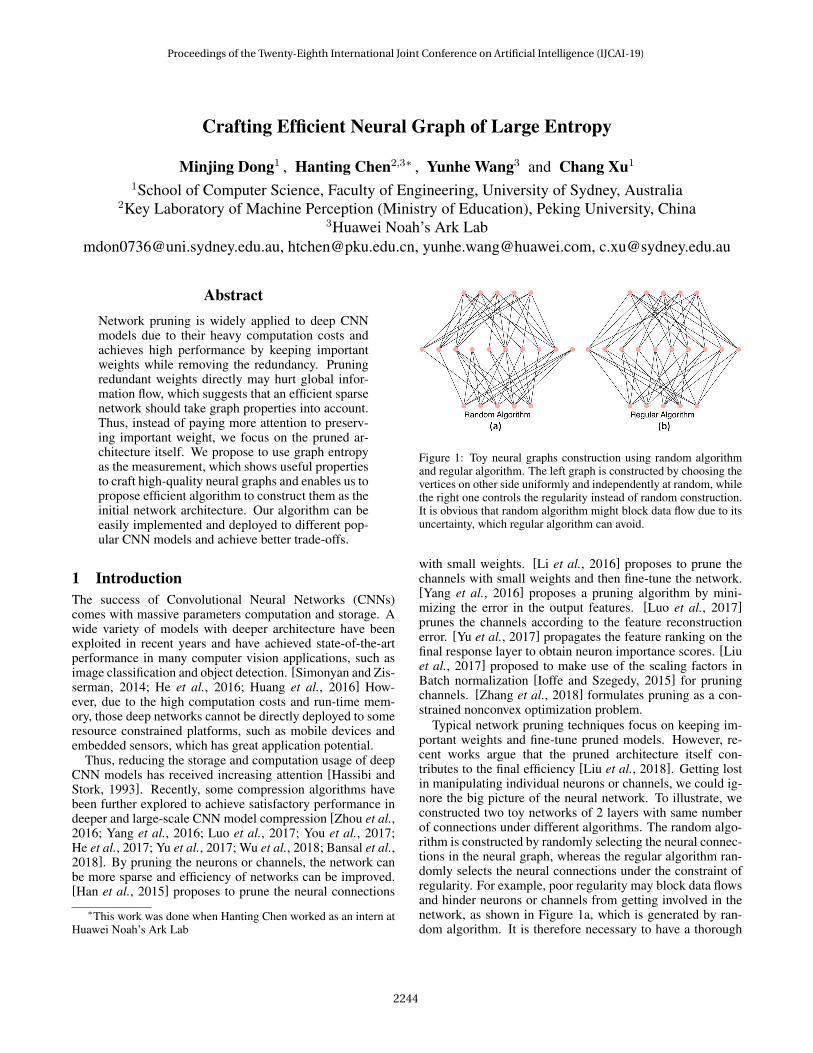
Figure 1: Toy neural graphs construction using random algorithmand regular algorithm. The left graph is constructed by choosing thevertices on other side uniformly and independently at random, whilethe right one controls the regularity instead of random construction.It is obvious that random algorithm might block data flow due to itsuncertainty, which regular algorithm can avoid.

with small weights. [Li et al., 2016] proposes to prune thechannels with small weights and then fine-tune the network.[Yang et al., 2016] proposes a pruning algorithm by mini-mizing the error in the output features. [Luo et al., 2017]prunes the channels according to the feature reconstructionerror. [Yu et al., 2017] propagates the feature ranking on thefinal response layer to obtain neuron importance scores. [Liuet al., 2017] proposed to make use of the scaling factors inBatch normalization [Ioffe and Szegedy, 2015] for pruningchannels. [Zhang et al., 2018] formulates pruning as a con-strained nonconvex optimization problem.

Typical network pruning techniques focus on keeping im-portant weights and fine-tune pruned models. However, re-cent works argue that the pruned architecture itself con-tributes to the final efficiency [Liu et al., 2018]. Getting lostin manipulating individual neurons or channels, we could ig-nore the big picture of the neural network. To illustrate, weconstructed two toy networks of 2 layers with same numberof connections under different algorithms. The random algo-rithm is constructed by randomly selecting the neural connec-tions in the neural graph, whereas the regular algorithm ran-domly selects the neural connections under the constraint ofregularity. For example, poor regularity may block data flowsand hinder neurons or channels from getting involved in thenetwork, as shown in Figure 1a, which is generated by ran-dom algorithm. It is therefore necessary to have a thorough

Proceedings of the Twenty-Eighth International Joint Conference on Artificial Intelligence (IJCAI-19)

2244

investigation on the characteristics displayed by the neuralnetwork as a whole (see Figure 1b), which forces all the ver-tices on the same side have similar degrees.

In this paper, we propose to craft efficient deep neural net-work through a graph lens. Structural complexity revealsthe way in which vertices and edges are arranged in thegraph, providing a significant influence on the graph functionand performance. Graph entropy offers an attractive routeto such complexity measures. To increase the capacity ofthe pruned network under a particular network sparsity, wemaximize graph entropy of the network by optimizing thearrangements of neurons and connections. We identify im-portant weights from the pre-trained over-parameterized net-work, and use them in preference to others in crafting our ef-ficient neural network. Based on the resulting sparse networkarchitecture, we train the network parameters from scratchrather than adapting their original weights. The proposed al-gorithm can be easily deployed to many popular network ar-chitectures, such as ResNet [He et al., 2016], VGG networks[Simonyan and Zisserman, 2014] and DenseNet [Huang etal., 2016]. Experimental results on ImageNet and CIFARdatasets [Krizhevsky, 2009; Deng et al., 2009] demonstratethat deep neural networks can be well compressed by investi-gating graph entropy while preserving the accuracy.

2 MethodologyPruning neural networks is to compresses networks by delet-ing neurons or neuron connections from a trained model,which has been paid more attention to in recent years. How-ever, most pruning techniques only involve local operationsand do not take whole network proprieties into consideration,which may block information flows from layer to layer. Incontrast, we take neural network architecture as a graph, andconstruct sparse graphs with a global viewpoint to initializethe network architecture before the training phase. To en-courage better information flow in the network, we employVon Neumann Entropy as a measurement to assess the qual-ities of graphs, which leads to a favorable tradeoff betweenaccuracy and sparsity of the neural network.

2.1 Von Neumann Entropy

Von Neumann Entropy is an extension of the Gibbs entropyto the quantum field, which can be treated as a quantita-tive measure of mixedness of density matrices [Braunsteinet al., 2004]. Recently, considering its capability of describ-ing spectral complexity, centrality, and entanglement of thegraph, Von Neumann Entropy has been further explored toevaluate graph entropy in various graph pattern recognitionand analysis applications. The definition of Von NeumannEntropy is given as

S(ρ) = −tr(ρ ln ρ), (1)

where tr denotes the trace of matrix and ρ is the density ma-trix. ρ could be a Laplacian matrix LG scaled by degree sumof graph G, i.e. ρ = 1

dGLG. Given λi as the i-th eigenvalue

of density matrix ρ, Von Neumann Entropy can be re-written

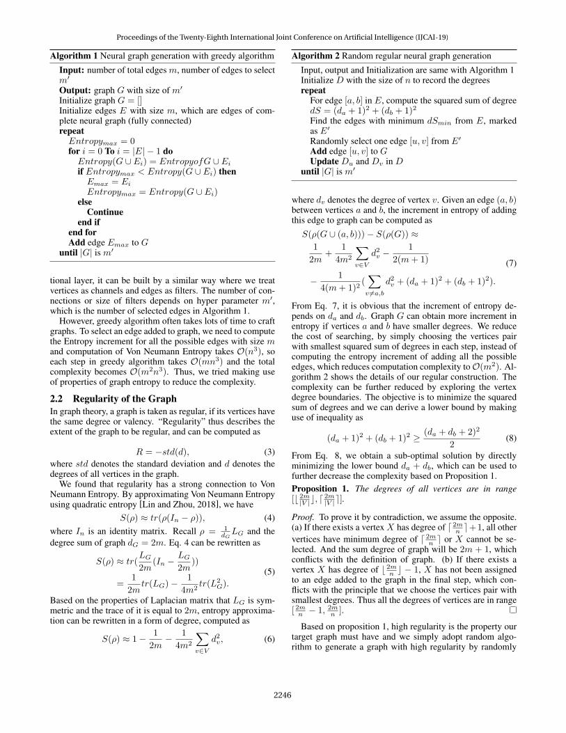
Figure 2: Neural graphs construction using greedy algorithm. Giventhe same number of edges, the left graph is the one with minimumentropy and the right one with maximum entropy. We can see thata graph with more fully-connected clusters tends to have small en-tropy and a well-balanced one tends to have large entropy.

in terms of spectrum of ρ as

S(ρ) = −n∑

i=1

λi lnλi. (2)

The Shannon entropy computes the uncertainty of globalspectral parameters of graph, involving all the eigenvalues,which makes it a useful and general measurement. Here wepay more attention to properties of Von Neumann Entropy.

To illustrate, we first constructed two toy graphs with theminimum and maximum entropy using greedy algorithm toexplore its properties, as shown in Figure 2. We observed thatgiven a fixed number of edges, if there are more connectedclusters that are disjoint unions of highly fully-connected sub-graph, the graph will have a smaller entropy. This is consis-tent with the results in [Passerini and Severini, 2008]. Theentropy of the graph in Figure 2 (a) is 2.554. Almost halfof connections from the first layer to bottom layer have beenblocked and several vertices are deactivated due to the min-imum entropy construction. On the contrary, a “balanced”graph that has a higher regularity tends to have a larger en-tropy. A more rigorous proof will be given later. For exam-ple, we plot a graph that is constructed with the maximum en-tropy given 50 edges in Figure 2 (b) whose entropy is 2.875.All vertices on the same layer have similar degree, which pro-duces a balanced graph and results in better connections anddata flows. If a graph is more balanced, every neuron wouldbe more active in contributing to the entire neural network,which results in a better network performance.

An efficient deep neural network is expected to have a bet-ter inner connection for data flows and high-sparsity for effi-cient compression, a graph of large entropy exactly tickes allthe boxes. Consider the neural graph G = (V,E), where Vis the set of vertices with size n and E is the set of edges withsize m. We can use greedy algorithm to maximize the en-tropy of graph. We simply compute graph entropy incrementby adding all the possible edges and select the one which con-tributes the maximum increment. Algorithm 1 shows the de-tails of it. After the neural graph construction, a network canbe easily crafted from the graph.

For a linear layer, it can easily built by treating verticesas neurons and edges as neuron connections. For a convolu-


2245

Algorithm 1 Neural graph generation with greedy algorithm

Input: number of total edges m, number of edges to selectm′

Output: graph G with size of m′

Initialize graph G = []Initialize edges E with size m, which are edges of com-plete neural graph (fully connected)repeatEntropymax = 0for i = 0 To i = |E| − 1 doEntropy(G ∪ Ei) = EntropyofG ∪ Ei

if Entropymax < Entropy(G ∪ Ei) thenEmax = Ei

Entropymax = Entropy(G ∪ Ei)else

Continueend if

end forAdd edge Emax to G

until |G| is m′

tional layer, it can be built by a similar way where we treatvertices as channels and edges as filters. The number of con-nections or size of filters depends on hyper parameter m′,which is the number of selected edges in Algorithm 1.

However, greedy algorithm often takes lots of time to craftgraphs. To select an edge added to graph, we need to computethe Entropy increment for all the possible edges with size mand computation of Von Neumann Entropy takes O(n3), soeach step in greedy algorithm takes O(mn3) and the totalcomplexity becomes O(m2n3). Thus, we tried making useof properties of graph entropy to reduce the complexity.

2.2 Regularity of the GraphIn graph theory, a graph is taken as regular, if its vertices havethe same degree or valency. “Regularity” thus describes theextent of the graph to be regular, and can be computed as

R = −std(d), (3)where std denotes the standard deviation and d denotes thedegrees of all vertices in the graph.

We found that regularity has a strong connection to VonNeumann Entropy. By approximating Von Neumann Entropyusing quadratic entropy [Lin and Zhou, 2018], we have

S(ρ) ≈ tr(ρ(In − ρ)), (4)where In is an identity matrix. Recall ρ = 1

dGLG and the

degree sum of graph dG = 2m. Eq. 4 can be rewritten as

S(ρ) ≈ tr(LG

2m(In −

LG

2m))

=1

2mtr(LG)−

1

4m2tr(L2

G).

(5)

Based on the properties of Laplacian matrix that LG is sym-metric and the trace of it is equal to 2m, entropy approxima-tion can be rewritten in a form of degree, computed as

S(ρ) ≈ 1− 1

2m− 1

4m2

∑v∈V

d2v, (6)

Algorithm 2 Random regular neural graph generation

Input, output and Initialization are same with Algorithm 1Initialize D with the size of n to record the degreesrepeat

For edge [a, b] in E, compute the squared sum of degreedS = (da + 1)2 + (db + 1)2

Find the edges with minimum dSmin from E, markedas E′

Randomly select one edge [u, v] from E′

Add edge [u, v] to GUpdate Du and Dv in D

until |G| is m′

where dv denotes the degree of vertex v. Given an edge (a, b)between vertices a and b, the increment in entropy of addingthis edge to graph can be computed as

S(ρ(G ∪ (a, b)))− S(ρ(G)) ≈1

2m+

1

4m2

∑v∈V

d2v −1

2(m+ 1)

− 1

4(m+ 1)2(∑v 6=a,b

d2v + (da + 1)2 + (db + 1)2).

(7)

From Eq. 7, it is obvious that the increment of entropy de-pends on da and db. Graph G can obtain more increment inentropy if vertices a and b have smaller degrees. We reducethe cost of searching, by simply choosing the vertices pairwith smallest squared sum of degrees in each step, instead ofcomputing the entropy increment of adding all the possibleedges, which reduces computation complexity toO(m2). Al-gorithm 2 shows the details of our regular construction. Thecomplexity can be further reduced by exploring the vertexdegree boundaries. The objective is to minimize the squaredsum of degrees and we can derive a lower bound by makinguse of inequality as

(da + 1)2 + (db + 1)2 ≥ (da + db + 2)2

2(8)

From Eq. 8, we obtain a sub-optimal solution by directlyminimizing the lower bound da + db, which can be used tofurther decrease the complexity based on Proposition 1.Proposition 1. The degrees of all vertices are in range[b 2m|V |c, d

2m|V |e].

Proof. To prove it by contradiction, we assume the opposite.(a) If there exists a vertexX has degree of d 2mn e+1, all othervertices have minimum degree of d 2mn e or X cannot be se-lected. And the sum degree of graph will be 2m + 1, whichconflicts with the definition of graph. (b) If there exists avertex X has degree of b 2mn c − 1, X has not been assignedto an edge added to the graph in the final step, which con-flicts with the principle that we choose the vertices pair withsmallest degrees. Thus all the degrees of vertices are in range[ 2mn − 1, 2mn ].

Based on proposition 1, high regularity is the property ourtarget graph must have and we simply adopt random algo-rithm to generate a graph with high regularity by randomly


2246

Figure 3: An illustration of our algorithm. Dotted lines denotes the complete neural graph and full ones denotes the edges added to the finalsparse graph. With importance weights, we add edges with maximum importance scores one by one to the graph. Meanwhile, we force theregularity of graph. For example, the edges with red values are the ones with top importance scores in the layer, however, those added tograph sometimes are not exactly these edges due to the regularity.

Algorithm 3 Regular neural graph generation with impor-tance weights

Input, output and Initialization are same with Algorithm 1Additional Input: importance scores SSort S in descending orderSort E according to Srepeat

Select edge [u, v] from E in orderif degree(u) < Umaxd

and degree(v) < Vmaxdthen

Add edge [u, v] to Gelse

Continueend if

until |G| is m′

adding edges to graph while restricting degree upper bound-ary of all the vertices, which reduces computation complexityto O(m). In terms of models which contains massive lay-ers and neural connections, we can simply divide the entirenetwork into several subnetworks, which further reduces thecomplexity of construction.

2.3 Importance WeightAlthough we reduce the construction complexity, the outputgraph is not fixed due to the random algorithm which ran-domly select the edge with minimum squared sum of degreesbecause there is no criterion for selection when the graph ex-ists multiple vertices pairs with minimum sum, which makesthe performance unstable, shown in Algorithm 2. Thus, weintroduce importance weights which can be easily obtainedto tackle this problem by giving the selection criterion.

Importance Estimation By GradientThe role of importance estimation is illustrated in Figure 3.Given the network N and input x, the output of network isN(x; θ), where θ denotes weight parameters of network. Theneuron connections (for FC layer) or filters (for CNN layer)may have different levels of importance according to the sen-sitivities of output to the infinitesimal changes on them. The

output difference under perturbation can be estimated by sim-ply computing the gradients of them as

N(x; θ + ε)−N(x; θ) ≈k∑ ∂(N(x; θ))

∂θiεi, (9)

where ε is the perturbation on weight parameters and k isthe number of parameters in the network. From Eq. 9, thesensitivity depends on the gradients of learned network withrespect to the weight parameters on input x. Thus, we canobtain estimated importance weights by computing their gra-dients as

S(θ) =1

M

M∑ ∂(N(xi; θ))

∂θ, (10)

where M is the number of examples from dataset. From Eq.10, importance weights can be computed by M times back-wards on a pre-trained model and selected dataset, which as-sists our initial sparse network to pay more attention to theseconnections with more important data flows.

Algorithm 3 shows the details of our proposed algorithm.With importance weights, we can construct the entire neu-ral graph with high regularity by adding edges one by oneaccording to their importance levels instead of random selec-tion algorithm, shown in Figure 3. Thus importance weightsguarantee that edges which tend to have important data flowwill be added to the graph, which makes the generated net-work adaptive to the specific dataset so that our network hasmore stable performance and gains better trade-offs.

Our final algorithm, regular algorithm with importanceweights (RAIW) has taken both graph entropy and impor-tance weights into consideration, which improves the effi-ciency due to graph entropy and guarantees the stability dueto importance weights. The entire process of crafting neuralgraphs is shown in Figure 3. The edges with high importancewill be added to our neural graph if it does not destroy theregularity of graph. For example, the edge with the top im-portance weights 0.01 cannot be added to our neural graphbecause it connects those vertices with higher degrees, thusthe edge with value of 0.005 is added instead, shown in thefinal step in Figure 3.


2247

3 ExperimentsTo evaluate the efficiency of our algorithms, we apply ourRAIW algorithm to generate neural graphs based on differ-ent popular CNN architectures, such as VGG, Resnet andDensenet. For comparison, we repeat the experiments on dif-ferent datasets, such as CIFAR10, CIFAR100 and Imagenet,with these architectures under various layer settings and com-pare them with pruning techniques or the original models todemonstrate better trade-offs of our algorithm. The stabilityand regularity will also be discussed.

3.1 Comparison With Efficient CNN ArchitecturesAnd Pruning Algorithms

VGG on CIFAR10We compare our algorithm against some popular pruningtechniques, [Han et al., 2015; Li et al., 2016; Liu et al., 2017][Liu et al., 2017] which achieve good performance amongpruning techniques. To evaluate the performance of RAIW,we evaluate on CIFAR10 [Krizhevsky, 2009] with VGG-16architecture. The detailed results are shown in Table 1. Ouralgorithm can preserve the accuracy, which has 0.6% drop butonly 1.1M parameters, almost 14X compression rate.

Densenet and Resnet on CIFAR100To evaluate the robustness of our algorithm, we deployRAIW on Densenet and Resnet running on CIFAR100 dataset[Krizhevsky, 2009]. We sparse these models by crafting con-volutional layers whose filter size is half of the original oneby controlling the number of selected edges in algorithms.

For Resnet on CIFAR100, we run Resnet with differentnumber of layers on CIFAR100 dataset. We compare ouralgorithm with these base models by comparing the 1-croperror along with the number of parameters of model, the de-tails are given in Figure 4 (a). Our algorithm consistentlyhas a better performance with the similar parameters, com-paring the two lines in Figure 4 (a). For example, the originalResnet-56 has 0.86M parameters number with 28.89% error,however, our RAIW algorithm which has the similar param-eter number on Resnet-110, has 0.8% error drop.

For Densenet on CIFAR100, we run with Densenet-BCwhich contains bottleneck layers and uses Densenet-BC-40-24, 40-48, 40-60 which have 40 layers and different growthrates as base models. Again, we show better accuracy-parameters trade-offs, the details are given in Figure 4 (b).Similarly, comparing the two lines in Figure 4 (b), the net-work we crafted using RAIW algorithm can be more effi-cient. For example, RAIW algorithm has 21.07% error on

Techniques Accuracy ParamsOriginal 94.0% 15.0M

[Li et al., 2016] 93.4% 5.4M[Liu et al., 2017] 93.8% 2.3M[Han et al., 2015] 93.3% 1.5M

RAIW 93.4% 1.1M

Table 1: The performance of VGG16 network crafted by RAIW al-gorithm compared with original VGG16 and pruning techniques onCIFAR 10 dataset.

Model Accuracy ParamsRAIW-Resnet-50 70.4% 13.28M

RAIW-Resnet-101 73.6% 21.08MResnet-34 73.3% 21.78MResnet-50 75.3% 25.50M

Table 2: The accuracy performance of Resnet crafted by RAIW eval-uated on Imagenet dataset, compared with original architectures, or-dered by number of parameters.

Densenet-BC-40-60 with 2.10M parameters while the origi-nal Densenet-BC-40-48 has 21.37% error with 2.76M param-eters, which demonstrates the efficiency of our algorithm.

Densenet and Resnet on ImagenetTo further evaluate the efficiency and generality of our algo-rithm, we also test on Imagenet [Deng et al., 2009] using theResnet and Densenet architectures crafted by our algorithm.

For Resnet on Imagenet, we craft Resnet-50 and 101 andcompare them to the original ones with similar parameternumbers. When the parameters number comes to 21M, ourRAIW algorithm on Resnet-101 can gain a slightly better ac-curacy than Resnet-34 with less parameters, shown in Table 2with bold. For Densenet on Imagenet, we craft Densenet-169,Densenet-201 and compare them to the original ones. Foreach Densenet model, RAIW has approximately 3% accu-racy drop but only 40% parameters of the original one. Thus,RAIW can obtain better accuracy-parameters trade-offs andimprove the efficiency of popular CNN architectures.

3.2 Stability Of ModelTo evaluate the stability of models under constructions of dif-ferent algorithms, we repeat the experiments on CIFAR10with VGG16 architecture. For each algorithm, we repeat 5times and compare their mean accuracy and standard devia-tion. We compare the regular algorithm 2 with RAIW 3 todemonstrate the role of importance weights.

The results are shown in Table 3, the random regular al-gorithm tends to have large variation on the accuracy due tothe random initial construction. Although they force graphsto be regular to different extents, there still exists high uncer-tainty because different connection distributions always havedifferent performance, which results in relatively high stan-dard deviation, shown in the first row with 0.17. In contrast,our RAIW algorithm has relatively high mean accuracy andlow standard deviation with 92.85 ± 0.12 (shown in the lastrow) because once the importance weights are computed, theneural graph is fixed, which makes the performance more sta-ble and the graph can be stored for multiple-times use, which

ALGO R1% R2% R3% R4% R5% AverageRegular 92.69 92.66 92.97 92.70 93.06 92.82±0.17RAIW 92.97 92.77 93.00 92.82 92.69 92.85±0.12

Table 3: VGG16 model under construction of regular algorithmand the one with importance weight over 5 runnings on CIFAR10dataset. The final column “Average” denotes the mean accuracy ±standard deviation.


2248

Figure 4: Trade-offs between number of parameters and error shown in (a) and (b). The orange lines denote error-parameters number trade-offs of our algorithm and the blue ones denote the original architecture. The two-line numbers on each data point in (a) denote the number oflayers in ResNet on the first line and the corresponding error on the second line. Those in (b) denote the number of layers in DenseNet withits growth rate on the first line and the corresponding error on the second line. We show the performance of our algorithm applied to Resneton CIFAR100 in (a), Densenet on CIFAR100 in (b). (c) illustrates entropy variation of 256*256 and 512*512 layers construction with degreeof 16. From the line chart, regular algorithm can guarantee much faster entropy increment compared with random algorithm.

VGG16 Original VGG d-32 VGG d-16 VGG d-8 VGGConv1 3x64x3x3 3x64x3x3 3x64x3x3 3x64x3x3Conv2 64x64x3x3 64x64x3x3 64x64x3x3 64x64x3x3Conv3 64x128x3x3 64x128x3x3 64x128x3x3 64x128x3x3Conv4 128x128x3x3 128x64x3x3 128x64x3x3 128x32x3x3Conv5 128x256x3x3 128x32x3x3 128x16x3x3 128x8x3x3Conv6 256x256x3x3 256x32x3x3 256x16x3x3 256x8x3x3Conv7 256x256x3x3 256x32x3x3 256x16x3x3 256x8x3x3Conv8 256x512x3x3 256x32x3x3 256x16x3x3 256x8x3x3Conv9 512x512x3x3 512x32x3x3 512x16x3x3 512x8x3x3

Conv10 512x512x3x3 512x32x3x3 512x16x3x3 512x8x3x3Conv11 512x512x3x3 512x32x3x3 512x16x3x3 512x16x3x3Conv12 512x512x3x3 512x32x3x3 512x16x3x3 512x16x3x3Conv13 512x512x3x3 512x32x3x3 512x16x3x3 512x16x3x3Linear1 512x512 512x128 512x128 512x64Linear2 512x10 512x10 512x10 512x10

Total 14.98M 1.07M 0.75M 0.55MAccuracy 93.96% 93.37% 93.06% 91.85%

Table 4: Details of each layer and number of parameters with accu-racy of VGG16 model under different sparsity.

saves the computation resources. Thus, RAIW algorithm im-proves the stability of regular algorithm, which makes it eas-ily deployable.

3.3 Role Of RegularityDue to regularity, d can be hyper parameters we use to spar-sify the network, where d denotes the degrees of all the ver-tices. And accuracy relies heavily on it due to the trade-offsbetween sparsity and performance. In this section, we runVGG16 model on CIFAR10 under different regularity to eval-uate trade-offs of our algorithms, as shown in Table 4.

We have tried 3 different sparsity, marked as d − 32, d −16, d − 8, and details of each layer are given in the Table4. Compared with original VGG16 architecture which gains93.86% accuracy with 14.98M parameters, our crafted neuralgraph d− 32 obtains “14x” compression rate with only 0.6%accuracy drop. Furthermore, d− 16 with “20x” compressionrate and d − 8 with “27x” compression rate, both have rela-

tively small accuracy drop.The reason why our constructed architecture allows high

sparsity is that our algorithm increment on graph entropy ismuch faster than other ones, as shown in Figure 4 (c). For thesimplicity, we construct two subnetworks and each of themcontains neural connections of two layers, which are 256∗256and 512 ∗ 512. The blue and green curves denote the entropyincrement along with the increasing of edge number underour algorithm 2 while the orange and red ones denote randomone. It is obvious that our algorithm keeps obtaining largeentropy increment during the edge construction. The graphentropy almost reaches its peak when we select d = 8 wherenumber of edges are 256 ∗ 8 = 2048 for 256*256 layer and512∗8 = 4096 for 512*512 layer. We found it interesting thatd = 8 is exactly the sparsity we have selected for d − 8 andthat’s the sparsity where we found the accuracy tends to havea relatively larger drop. Thus, we believe that the accuracyis highly related to entropy value. As a result, our algorithmguarantees maximum increment of entropy so that it can gainlarge entropy with less edges, which enables our model tohave high sparsity.

4 ConclusionNotice the strong connection between nerual networks andgraphs, we tried to improve the efficiency by construct neuralgraphs which have better vertices and connections arrange-ment. Thus, we propose to craft efficient neural networksbased on the properties of graph entropy. We reduce the com-putation complexity of graph generation to make it deploy-able and make use of importance weights to guarantee stabil-ity. Our RAIW algorithm achieves better trade-offs comparedto pruning algorithms and efficient CNN architectures.

AcknowledgementsThis work was supported in part by the Australian ResearchCouncil under Project DE180101438.


2249

References[Bansal et al., 2018] Nitin Bansal, Xiaohan Chen, and

Zhangyang Wang. Can we gain more from orthogonal-ity regularizations in training deep networks? In Advancesin Neural Information Processing Systems, pages 4261–4271, 2018.

[Braunstein et al., 2004] Samuel Braunstein, SibasishGhosh, and Simone Severini. The laplacian of a graphas a density matrix: A basic combinatorial approach toseparability of mixed states. Annals of Combinatorics, 10,07 2004.

[Deng et al., 2009] J. Deng, W. Dong, R. Socher, L.-J. Li,K. Li, and L. Fei-Fei. ImageNet: A Large-Scale Hierar-chical Image Database. In CVPR09, 2009.

[Han et al., 2015] Song Han, Jeff Pool, John Tran, andWilliam J. Dally. Learning both weights and connec-tions for efficient neural networks. CoRR, abs/1506.02626,2015.

[Hassibi and Stork, 1993] Babak Hassibi and David G.Stork. Second order derivatives for network pruning: Opti-mal brain surgeon. In S. J. Hanson, J. D. Cowan, and C. L.Giles, editors, Advances in Neural Information ProcessingSystems 5, pages 164–171. Morgan-Kaufmann, 1993.

[He et al., 2016] Kaiming He, Xiangyu Zhang, ShaoqingRen, and Jian Sun. Identity mappings in deep residualnetworks. CoRR, abs/1603.05027, 2016.

[He et al., 2017] Yihui He, Xiangyu Zhang, and Jian Sun.Channel pruning for accelerating very deep neural net-works. CoRR, abs/1707.06168, 2017.

[Huang et al., 2016] Gao Huang, Zhuang Liu, and Kilian Q.Weinberger. Densely connected convolutional networks.CoRR, abs/1608.06993, 2016.

[Ioffe and Szegedy, 2015] Sergey Ioffe and ChristianSzegedy. Batch normalization: Accelerating deep net-work training by reducing internal covariate shift. CoRR,abs/1502.03167, 2015.

[Krizhevsky, 2009] Alex Krizhevsky. Learning multiple lay-ers of features from tiny images. 2009.

[Li et al., 2016] Hao Li, Asim Kadav, Igor Durdanovic,Hanan Samet, and Hans Peter Graf. Pruning filters forefficient convnets. CoRR, abs/1608.08710, 2016.

[Lin and Zhou, 2018] Hongying Lin and Bo Zhou. On thevon neumann entropy of a graph. Discrete Applied Math-ematics, 247:448 – 455, 2018.

[Liu et al., 2017] Zhuang Liu, Jianguo Li, Zhiqiang Shen,Gao Huang, Shoumeng Yan, and Changshui Zhang.Learning efficient convolutional networks through net-work slimming. CoRR, abs/1708.06519, 2017.

[Liu et al., 2018] Zhuang Liu, Mingjie Sun, Tinghui Zhou,Gao Huang, and Trevor Darrell. Rethinking the value ofnetwork pruning. CoRR, abs/1810.05270, 2018.

[Luo et al., 2017] Jian-Hao Luo, Jianxin Wu, and WeiyaoLin. Thinet: A filter level pruning method for deep neuralnetwork compression. CoRR, abs/1707.06342, 2017.

[Passerini and Severini, 2008] Filippo Passerini and SimoneSeverini. The von neumann entropy of networks. Univer-sity Library of Munich, Germany, MPRA Paper, 12 2008.

[Simonyan and Zisserman, 2014] Karen Simonyan and An-drew Zisserman. Very deep convolutional networks forlarge-scale image recognition. CoRR, abs/1409.1556,2014.

[Wu et al., 2018] Junru Wu, Yue Wang, Zhenyu Wu,Zhangyang Wang, Ashok Veeraraghavan, and YingyanLin. Deep k-means: Re-training and parameter sharingwith harder cluster assignments for compressing deep con-volutions. CoRR, abs/1806.09228, 2018.

[Yang et al., 2016] Tien-Ju Yang, Yu-Hsin Chen, and Vivi-enne Sze. Designing energy-efficient convolutionalneural networks using energy-aware pruning. CoRR,abs/1611.05128, 2016.

[You et al., 2017] Shan You, Chang Xu, Chao Xu, andDacheng Tao. Learning from multiple teacher networks. InProceedings of the 23rd ACM SIGKDD International Con-ference on Knowledge Discovery and Data Mining, KDD’17, pages 1285–1294, New York, NY, USA, 2017. ACM.

[Yu et al., 2017] Ruichi Yu, Ang Li, Chun-Fu Chen, Jui-Hsin Lai, Vlad I. Morariu, Xintong Han, Mingfei Gao,Ching-Yung Lin, and Larry S. Davis. NISP: pruning net-works using neuron importance score propagation. CoRR,abs/1711.05908, 2017.

[Zhang et al., 2018] Tianyun Zhang, Shaokai Ye, KaiqiZhang, Jian Tang, Wujie Wen, Makan Fardad, and YanzhiWang. A systematic DNN weight pruning framework us-ing alternating direction method of multipliers. CoRR,abs/1804.03294, 2018.

[Zhou et al., 2016] Hao Zhou, Jose M. Alvarez, and FatihPorikli. Less is more: Towards compact cnns. In BastianLeibe, Jiri Matas, Nicu Sebe, and Max Welling, editors,Computer Vision – ECCV 2016, pages 662–677, Cham,2016. Springer International Publishing.


2250

crafting efficient neural graph of large entropy

Documents