Flish

a Fe

rnandez

1

DATA MINING

2

Em

ily T

hom

as, S

tate

Univ

ersity

of N

ew

Yo

rk

WHAT IS DATA MINING?

Data Mining is the discovery of hidden knowledge, unexpected patterns and new rules in large databases

Automating the process of searching patterns in the data

3

anderso

n.u

cla.e

du

OBJECTIVE OF DATA MINING

Any of four types of relationships are sought: Classes – stored data is used to locate data in

predetermined groups Clusters – data items grouped according to

logical relationships or consumer preferences Associations – Walmart example (beer and

diapers) Sequential Patterns – data mined to anticipate

behavior patterns and trends

4

Em

ily T

hom

as, S

tate

Univ

ersity

of N

ew

Yo

rk

DATA MINING TECHNIQUES

Rule Induction – extraction of if-then rules Nearest Neighbors Artificial Neural Networks – models that learn Clustering Genetic Algorithms – concept of natural

evolution Factor Analysis Exploratory Stepwise Regression Data Visualization – usage of graphic tools Decision Trees

5

Flish

a Fe

rnandez

CLASSIFICATION

A major data mining operation Given one attribute (e.g. Wealth), try to to

predict the value of new people’s wealths by means of some of the other available attributes

Applies to categorical outputs

Categorical attribute: an attribute which takes on two or more discrete values, also knows as a symbolic attribute

Real attribute: a column of real numbers, also known as a continuous attribute

6

DATASET

Kohavi 1

99

5

symbolreal classification

7

DECISION TREES

Flish

a Fe

rnandez

8

anderso

n.u

cla.e

du / W

ikipedia

DECISION TREES

Also called classification trees or regression trees

Based on recursive partitioning of the sample space

Tree-shaped structures that represent sets of decisions/data which generate rules for the classification of a (new, unclassified) dataset

The resulting classification tree becomes an input for decision making

9

Learn

ing D

ecisio

n Tre

es

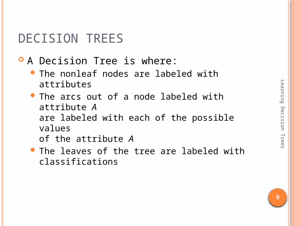
DECISION TREES

A Decision Tree is where: The nonleaf nodes are labeled with attributes The arcs out of a node labeled with attribute A

are labeled with each of the possible values of the attribute A

The leaves of the tree are labeled with classifications

10

Wik

ipedia

ADVANTAGES

Simple to understand and interpret Requires little data preparation (other

techniques need data normalization, dummy variables, etc.)

Can support both numerical and categorical data

Uses white box model (explained by boolean logic)

Reliable – possible to validate model using statistical tests

Robust – large amounts of data can be analyzed in a short amount of time

11

DECISION TREE EXAMPLE

Flish

a Fe

rnandez

12

From

Wik

ipedia

DAVID’S DEBACLE

Status Quo: Sometimes people play golf, sometimes they do not

Objective: Come up with optimized staff schedule

Means: Predict when people will play golf, when they will not

13

Quin

lan 1

98

9

DAVID’S DATASETOutlook Temp Humidity Windy Play

Sunny 85 85 No No

Sunny 80 90 Yes No

Overcast 83 78 No Yes

Rain 70 96 No Yes

Rain 68 80 No Yes

Rain 65 70 Yes No

Overcast 64 65 Yes Yes

Sunny 72 95 No No

Sunny 69 70 No Yes

Rain 75 90 No Yes

Sunny 75 70 Yes Yes

Overcast 72 90 Yes Yes

Overcast 81 75 No Yes

Rain 71 80 Yes No

14

From

Wik

ipedia

DAVID’S DIAGRAM

Play: 9Don’t: 5

SUNNYPlay: 2

Don’t: 3

HUMIDITY <= 70Play: 2

Don’t: 0

HUMIDITY > 70Play: 0

Don’t: 3

OVERCASTPlay: 4

Don’t: 0

RAINPlay: 3

Don’t: 2

WINDYPlay: 0Don’t:

2

NOT WINDYPlay: 3

Don’t: 0

outlook?

windy?

humid?

15

Flish

a Fe

rnandez

DAVID’S DECISION TREE

Outlook?

Humidity?

PlayDon’

t Play

Play Windy?

PlayDon’

t Play

Sunny

Overcast

Rain

HighNormal TrueFalse

Non-leaf NodesLabeled with Attributes

Leaves Labeled with Classifications

Arcs Labeled with Possible Values

Root Node

16

From

Wik

ipedia

DAVID’S DECISION

Dismiss staff when it is Sunny AND Hot Rainy AND Windy

Hire extra staff when it is Cloudy Sunny AND Not So Hot Rainy AND Not Windy

Flish

a Fe

rnandez

17

DECISION TREE INDUCTION

18

DECISION TREE INDUCTION ALGORITHM

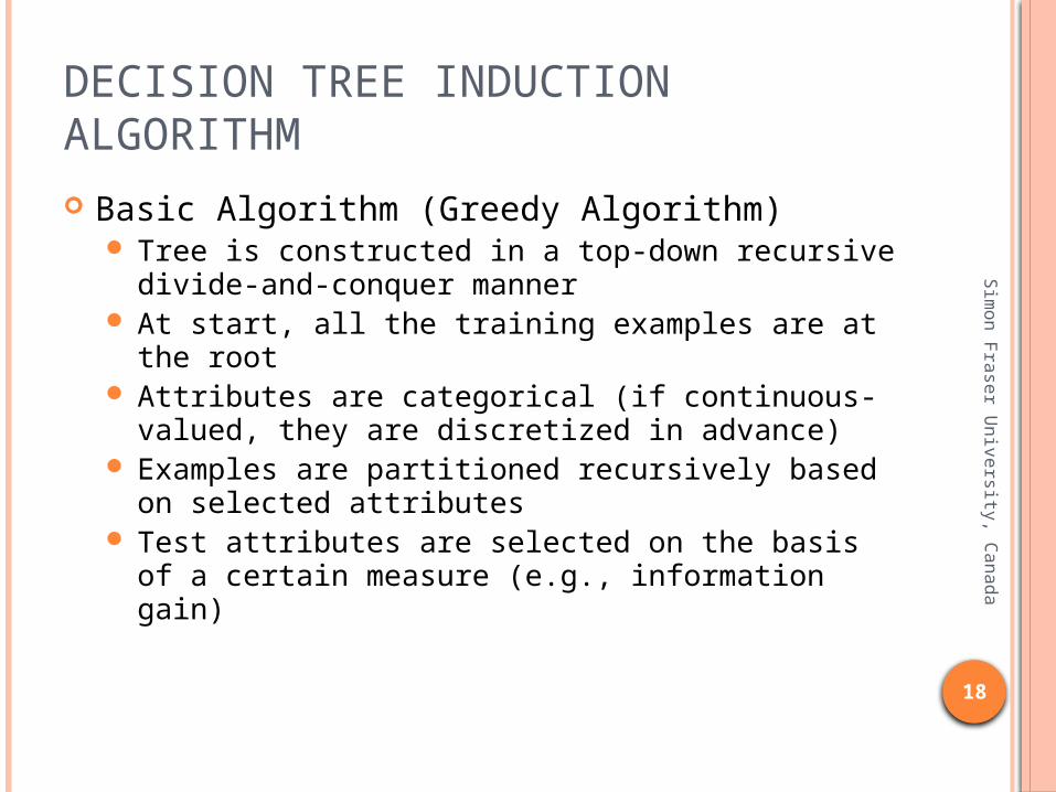
Basic Algorithm (Greedy Algorithm) Tree is constructed in a top-down recursive divide-

and-conquer manner At start, all the training examples are at the root Attributes are categorical (if continuous-valued,

they are discretized in advance) Examples are partitioned recursively based on

selected attributes Test attributes are selected on the basis of a certain

measure (e.g., information gain)

Sim

on Fra

ser U

niv

ersity

, Canada

19

Decisio

n Tre

e Le

arn

ing

ISSUES

How should the attributes be split? What is the appropriate root? What is the best split?

When should we stop splitting? Should we prune?

20

DB

MS D

ata

Min

ing S

olu

tions S

upple

me

nt

TWO PHASES

Tree Growing (Splitting) Splitting data into progressively smaller subsets Analyzing the data to find the independent

variable (such as outlook, humidity, windy) that when used as a splitting rule will result in nodes that are most different from each other with respect to the dependent variable (play)

Tree Pruning

21

Flish

a Fe

rnandez

SPLITTING

22

DB

MS D

ata

Min

ing S

olu

tions S

upple

me

nt

SPLITTING ALGORITHMS

Random Information Gain Information Gain Ratio GINI Index

23

DATASET

AIX

plo

rato

rium

24

RANDOM SPLITTING

AIX

plo

rato

rium

25

RANDOM SPLITTING

Disadvantages Trees can grow huge Hard to understand Less accurate than smaller trees

AIX

plo

rato

rium

26

DB

MS D

ata

Min

ing S

olu

tions S

upple

me

nt

SPLITTING ALGORITHMS

Random Information Gain Information Gain Ratio GINI Index

27

Wik

ipedia

INFORMATION ENTROPY

A measure of the uncertainty associated with a random variable

A measure of the average information content the recipient is missing when they do not know the value of the random variable

A long string of repeating characters has an entropy of 0, since every character is predictable

Example: Coin Toss Independent fair coin flips have an entropy of 1

bit per flip A double-headed coin has an entropy of 0 – each

toss of the coin delivers no information

1),()(

iii

ii npInp

npAE

28

Wik

ipedia

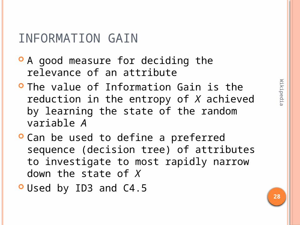
INFORMATION GAIN

A good measure for deciding the relevance of an attribute

The value of Information Gain is the reduction in the entropy of X achieved by learning the state of the random variable A

Can be used to define a preferred sequence (decision tree) of attributes to investigate to most rapidly narrow down the state of X

Used by ID3 and C4.5

29

Flish

a Fe

rnandez

CALCULATING INFORMATION GAIN

First compute information content

Ex. Attribute Thread = New, Skips = 3, Reads = 7 -0.3 * log 0.3 - 0.7 * log 0.7 = 0.881 (using log base 2)

Ex. Attribute Thread = Old, Skips = 6, Reads = 2 -0.6 * log 0.6 - 0.2 * log 0.2 = 0.811 (using log base 2)

Information Gain is... Of 18, 10 threads are new and 8 threads are old 1.0 - (10/18)*0.881 + (8/18)*0.811 0.150

npn

npn

npp

npp

npI

22 loglog),(

)(),()( AEnpIAGain

30

INFORMATION GAIN

AIX

plo

rato

rium

31

TEST DATA

Where

When

Fred Starts

Joe Offense

Joe Defense

Opp C

Outcome

Away 9pm No Center Forward Tall ??

AIX

plo

rato

rium

32

DRAWBACKS OF INFORMATION GAIN

Prefers attributes with many values (real attributes) Prefers AudienceSize {1,2,3,..., 150, 151, ...,

1023, 1024, ... } But larger attributes are not necessarily better

Example: credit card number Has a high information gain because it uniquely

identifies each customer But deciding how to treat a customer based on

their credit card number is unlikely to generalize customers we haven't seen before

Wik

ipedia

/ AIX

plo

rato

rium

33

DB

MS D

ata

Min

ing S

olu

tions S

upple

me

nt

SPLITTING ALGORITHMS

Random Information Information Gain Ratio GINI Index

34

INFORMATION GAIN RATIO

Works by penalizing multiple-valued attributes

Gain ratio should be Large when data is evenly spread Small when all data belong to one branch

Gain ratio takes number and size of branches into account when choosing an attribute It corrects the information gain by taking the

intrinsic information of a split into account (i.e. how much info do we need to tell which branch an instance belongs to)

http

://ww

w.it.iitb

.ac.in

/~su

nita

35

http

://ww

w.it.iitb

.ac.in

/~su

nita

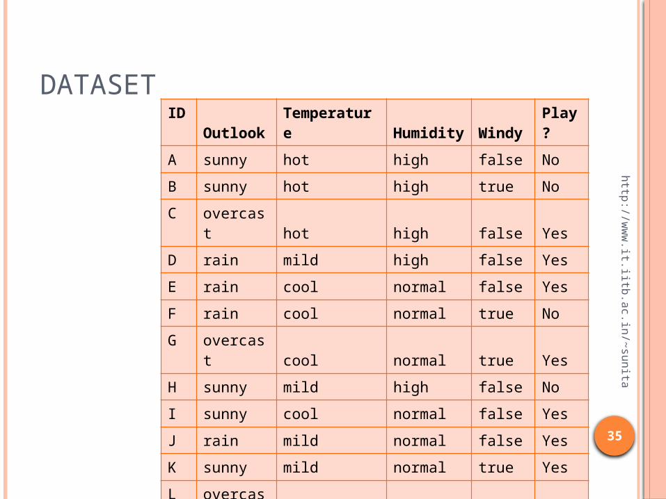
DATASETID

OutlookTemperature

Humidity

Windy

Play?

A sunny hot high false No

B sunny hot high true No

C overcast hot high false Yes

D rain mild high false Yes

E rain cool normal false Yes

F rain cool normal true No

G overcast cool normal true Yes

H sunny mild high false No

I sunny cool normal false Yes

J rain mild normal false Yes

K sunny mild normal true Yes

L overcast mild high true Yes

M overcast hot normal false Yes

N rain mild high true No

36

http

://ww

w.it.iitb

.ac.in

/~su

nita

CALCULATING GAIN RATIO

Intrinsic information: entropy of distribution of instances into branches

Gain ratio (Quinlan’86) normalizes info gain by

.||

||2

log||||

),(SiS

SiSASnfoIntrinsicI

.),(

),(),(ASnfoIntrinsicI

ASGainASGainRatio

37

http

://ww

w.it.iitb

.ac.in

/~su

nita

COMPUTING GAIN RATIO Example: intrinsic information for ID code

Importance of attribute decreases as intrinsic information gets larger

Example of gain ratio:

bits 807.3)14/1log14/1(14),1[1,1,(info

)Attribute"info("intrinsic_)Attribute"gain("

)Attribute"("gain_ratio

246.0bits 3.807bits 0.940

)ID_code"("gain_ratio

38

http

://ww

w.it.iitb

.ac.in

/~su

nita

DATASETID

OutlookTemperature

Humidity

Windy

Play?

A sunny hot high false No

B sunny hot high true No

C overcast hot high false Yes

D rain mild high false Yes

E rain cool normal false Yes

F rain cool normal true No

G overcast cool normal true Yes

H sunny mild high false No

I sunny cool normal false Yes

J rain mild normal false Yes

K sunny mild normal true Yes

L overcast mild high true Yes

M overcast hot normal false Yes

N rain mild high true No

39

http

://ww

w.it.iitb

.ac.in

/~su

nita

INFORMATION GAIN RATIOS

Outlook Temperature

Info: 0.693 Info: 0.911

Gain: 0.940-0.693 0.247 Gain: 0.940-0.911 0.029

Split info: info([5,4,5]) 1.577 Split info: info([4,6,4])

1.362

Gain ratio: 0.247/1.577

0.156 Gain ratio: 0.029/1.362

0.021

Humidity Windy

Info: 0.788 Info: 0.892

Gain: 0.940-0.788 0.152 Gain: 0.940-0.892 0.048

Split info: info([7,7]) 1.000 Split info: info([8,6]) 0.985

Gain ratio: 0.152/1 0.152 Gain ratio: 0.048/0.985

0.049

40

http

://ww

w.it.iitb

.ac.in

/~su

nita

MORE ON GAIN RATIO

“Outlook” still comes out top However, “ID code” has greater gain ratio

Standard fix: ad hoc test to prevent splitting on that type of attribute

Problem with gain ratio: it may overcompensate May choose an attribute just because its intrinsic

information is very low Standard fix:

First, only consider attributes with greater than average information gain

Then, compare them on gain ratio

41

INFORMATION GAIN RATIO

Below is the decision tree

AIX

plo

rato

rium

42

TEST DATA

Where

When

Fred Starts

Joe Offense

Joe Defense

Opp C

Outcome

Away 9pm No Center Forward Tall ??

AIX

plo

rato

rium

43

DB

MS D

ata

Min

ing S

olu

tions S

upple

me

nt

SPLITTING ALGORITHMS

Random Information Information Gain Ratio GINI Index

44

GINI INDEX

All attributes are assumed continuous-valued

Assumes there exist several possible split values for each attribute

May need other tools, such as clustering, to get the possible split values

Can be modified for categorical attributes

Used in CART, SLIQ, SPRINT

Flish

a Fe

rnandez

45

khch

o@

dbla

b.cb

u.a

c.kr

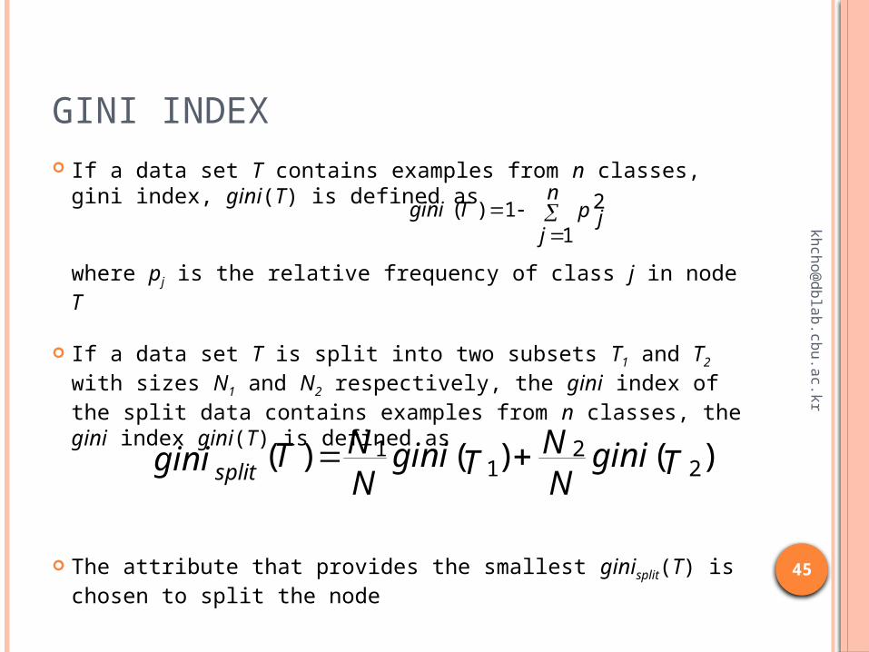
GINI INDEX If a data set T contains examples from n classes, gini

index, gini(T) is defined as

where pj is the relative frequency of class j in node T

If a data set T is split into two subsets T1 and T2 with sizes N1 and N2 respectively, the gini index of the split data contains examples from n classes, the gini index gini(T) is defined as

The attribute that provides the smallest ginisplit(T) is chosen to split the node

n

jp jTgini

1

21)(

)()()( 22

11 Tgini

NN

TginiNNTginisplit

46

khch

o@

dbla

b.cb

u.a

c.kr

GINI INDEX

Maximum (1 - 1/nc) when records are equally distributed among all classes, implying least interesting information

Minimum (0.0) when all records belong to one class, implying most interesting information

C1 0C2 6

Gini=0.000

C1 2C2 4

Gini=0.444

C1 3C2 3

Gini=0.500

C1 1C2 5

Gini=0.278

47

khch

o@

dbla

b.cb

u.a

c.kr

EXAMPLES FOR COMPUTING GINI

j

tjptGINI 2)]|([1)(

C1 0 C2 6

C1 2 C2 4

C1 1 C2 5

P(C1) = 0/6 = 0 P(C2) = 6/6 = 1

Gini = 1 – P(C1)2 – P(C2)2 = 1 – 0 – 1 = 0

P(C1) = 1/6 P(C2) = 5/6

Gini = 1 – (1/6)2 – (5/6)2 = 0.278

P(C1) = 2/6 P(C2) = 4/6

Gini = 1 – (2/6)2 – (4/6)2 = 0.444

48

DB

MS D

ata

Min

ing S

olu

tions S

upple

me

nt / A

I Depot

STOPPING RULES

Pure nodes Maximum tree depth, or maximum number

of nodes in a tree Because of overfitting problems

Minimum number of elements in a node considered for splitting, or its near equivalent

Minimum number of elements that must be in a new node

A threshold for the purity measure can be imposed such that if a node has a purity value higher than the threshold, no partitioning will be attempted regardless of the number of observations

49

Flish

a Fe

rnandez

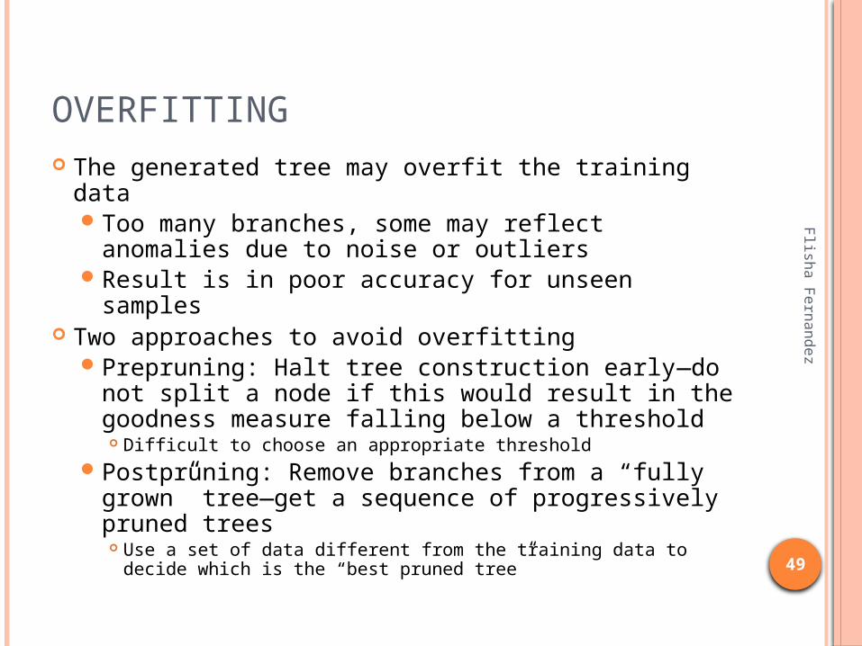
OVERFITTING The generated tree may overfit the training data

Too many branches, some may reflect anomalies due to noise or outliers

Result is in poor accuracy for unseen samples Two approaches to avoid overfitting

Prepruning: Halt tree construction early—do not split a node if this would result in the goodness measure falling below a threshold Difficult to choose an appropriate threshold

Postpruning: Remove branches from a “fully grown” tree—get a sequence of progressively pruned trees Use a set of data different from the training data to decide

which is the “best pruned tree”

50

DB

MS D

ata

Min

ing S

olu

tions S

upple

me

nt

PRUNING

Used to make a tree more general, more accurate

Removes branches that reflect noise

51

Flish

a Fe

rnandez

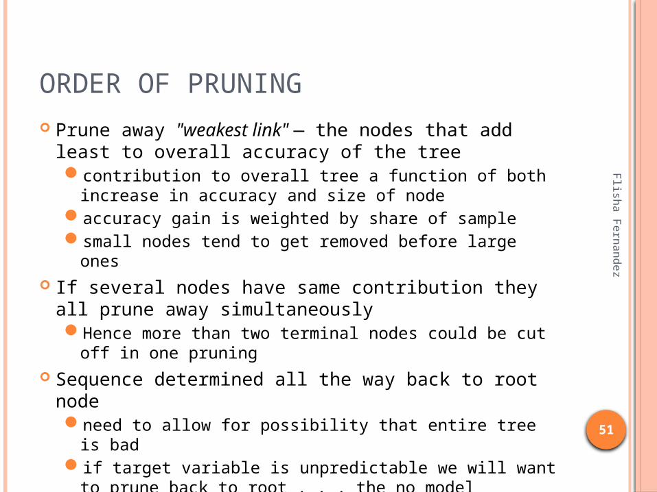
ORDER OF PRUNING Prune away "weakest link" — the nodes that add least

to overall accuracy of the treecontribution to overall tree a function of both increase in

accuracy and size of node accuracy gain is weighted by share of samplesmall nodes tend to get removed before large ones

If several nodes have same contribution they all prune away simultaneouslyHence more than two terminal nodes could be cut off in

one pruning Sequence determined all the way back to root node

need to allow for possibility that entire tree is badif target variable is unpredictable we will want to prune

back to root . . . the no model solution

52

CROSS-VALIDATION

Of the training sample, give learner only a subset Ex: Training on the first 15 games, testing on the

last 5 Gives us a measure of the quality of the

decision trees produced based on their splitting algorithm

Remember that more examples lead to better estimates

AIX

plo

rato

rium

Flish

a Fe

rnandez

53

ALGORITHMS

54

anderso

n.u

cla.e

du

DECISION TREE METHODS

ID3 and C4.5 Algorithms Developed by Ross Quinlan

Classification and Regression Trees (CART) Segments a dataset using 2-way splits

Chi Square Automatic Interaction Detection (CHAID) Segments a dataset using chi square tests to

create multi-way splits And many others

55

Wik

ipedia

ID3 ALGORITHM

Developed by Ross Quinlan Iterative Dichotomiser 3 Based on Occam’s Razor Prefers smaller decision trees over larger

ones Does not always produce the smallest tree, is

heuristic Summarized as follows:

Take all unused attributes and count their entropy concerning test samples

Choose attribute for which entropy is minimum Make node containing that attribute

56

Wik

ipedia

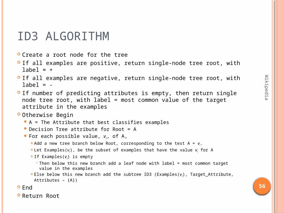
ID3 ALGORITHM Create a root node for the tree If all examples are positive, return single-node tree root, with label = + If all examples are negative, return single-node tree root, with label = - If number of predicting attributes is empty, then return single node

tree root, with label = most common value of the target attribute in the examples

Otherwise Begin A = The Attribute that best classifies examples Decision Tree attribute for Root = A For each possible value, vi, of A,

Add a new tree branch below Root, corresponding to the test A = vi. Let Examples(vi), be the subset of examples that have the value vi for A If Examples(vi) is empty

Then below this new branch add a leaf node with label = most common target value in the examples

Else below this new branch add the subtree ID3 (Examples(vi), Target_Attribute, Attributes – {A})

End Return Root

57

http

://ww

w.cse

.unsw

.edu.a

u/

EXAMPLE DATA

Size Color Shape Class

Medium Blue Brick Yes

Small Red Sphere Yes

Large Green Pillar Yes

Large Green Sphere Yes

Small Red Wedge No

Large Red Wedge No

Large Red Pillar No

58

http

://ww

w.cse

.unsw

.edu.a

u/

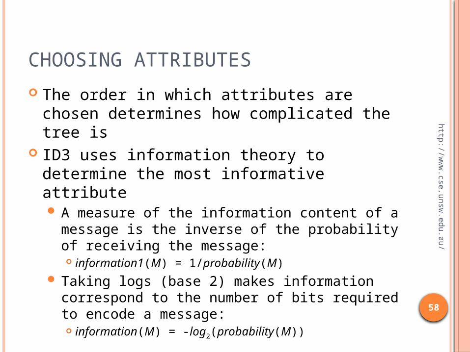
CHOOSING ATTRIBUTES

The order in which attributes are chosen determines how complicated the tree is

ID3 uses information theory to determine the most informative attribute A measure of the information content of a

message is the inverse of the probability of receiving the message: information1(M) = 1/probability(M)

Taking logs (base 2) makes information correspond to the number of bits required to encode a message: information(M) = -log2(probability(M))

59

http

://ww

w.cse

.unsw

.edu.a

u/

INFORMATION

The information content of a message should be related to the degree of surprise in receiving the message

Messages with a high probability of arrival are not as informative as messages with low probability

Learning aims to predict accurately, i.e. reduce surprise

Probabilities are multiplied to get the probability of two or more things both/all happening. Taking logarithms of the probabilities allows information to be added instead of multiplied

60

http

://ww

w.cse

.unsw

.edu.a

u/

ENTROPY

Different messages have different probabilities of arrival

Overall level of uncertainty (termed entropy) is: -Σi Pi log2Pi

Frequency can be used as a probability estimate e.g. if there are 5 positive examples and 3

negative examples in a node the estimated probability of positive is 5/8 = 0.625

61

http

://ww

w.cse

.unsw

.edu.a

u/

LEARNING

Learning tries to reduce the information content of the inputs by mapping them to fewer outputs

Hence we try to minimize entropy

62

http

://ww

w.cse

.unsw

.edu.a

u/

SPLITTING CRITERION

Work out entropy based on distribution of classes

Trying splitting on each attribute Work out expected information gain for each

attribute Choose best attribute

63

http

://ww

w.cse

.unsw

.edu.a

u/

EXAMPLE DATA

Size Color Shape Class

Medium Blue Brick Yes

Small Red Sphere Yes

Large Green Pillar Yes

Large Green Sphere Yes

Small Red Wedge No

Large Red Wedge No

Large Red Pillar No

64

http

://ww

w.cse

.unsw

.edu.a

u/

EXAMPLE

Initial decision tree is one node with all examples.

There are 4 positive examples and 3 negative examples i.e. probability of positive is 4/7 = 0.57;

probability of negative is 3/7 = 0.43 Entropy for Examples is: – (0.57 * log 0.57) –

(0.43 * log 0.43) = 0.99 Evaluate possible ways of splitting

65

http

://ww

w.cse

.unsw

.edu.a

u/

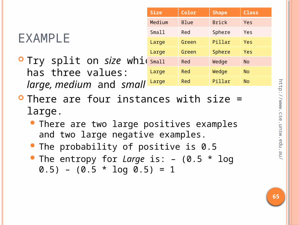
EXAMPLE

Try split on size which has three values: large, medium and small

There are four instances with size = large. There are two large positives examples and two

large negative examples. The probability of positive is 0.5 The entropy for Large is: – (0.5 * log 0.5) – (0.5 *

log 0.5) = 1

Size Color Shape Class

Medium Blue Brick Yes

Small Red Sphere Yes

Large Green Pillar Yes

Large Green Sphere Yes

Small Red Wedge No

Large Red Wedge No

Large Red Pillar No

66

http

://ww

w.cse

.unsw

.edu.a

u/

EXAMPLE

There is one small positive and one small negative Entropy for Small is:

– (0.5 * log 0.5) – (0.5 * log 0.5) = 1

There is only one medium positive and no medium negatives Entropy for Medium is 0

Expected information for a split on Size is:

Size Color Shape Class

Medium Blue Brick Yes

Small Red Sphere Yes

Large Green Pillar Yes

Large Green Sphere Yes

Small Red Wedge No

Large Red Wedge No

Large Red Pillar No

Size Color Shape Class

Medium Blue Brick Yes

Small Red Sphere Yes

Large Green Pillar Yes

Large Green Sphere Yes

Small Red Wedge No

Large Red Wedge No

Large Red Pillar No

67

http

://ww

w.cse

.unsw

.edu.a

u/

EXAMPLE

The expected information gain for Size is: 0.99 – 0.86 = 0.13

Checking the Information Gains on color and shape: Color has an information gain of 0.52 Shape has an information gain of 0.7

Therefore split on shape Repeat for all subtrees

68

http

://ww

w.cse

.unsw

.edu.a

u/

OUTPUT TREE

69

http

://ww

w.cse

.unsw

.edu.a

u/

WINDOWING

ID3 can deal with very large data sets by performing induction on subsets or windows onto the data1. Select a random subset of the whole set of

training instances2. Use the induction algorithm to form a rule to

explain the current window3. Scan through all of the training instances

looking for exceptions to the rule4. Add the exceptions to the window

Repeat steps 2 to 4 until there are no exceptions left

70

http

://ww

w.cse

.unsw

.edu.a

u/

NOISY DATA Frequently, training data contains "noise" (examples

which are misclassified) In such cases, one is like to end up with a part of the

decision tree which considers say 100 examples, of which 99 are in class C1 and the other is apparently in class C2

If there are any unused attributes, we might be able to use them to elaborate the tree to take care of this one case, but the subtree we would be building would in fact be wrong, and would likely misclassify real data

Thus, particularly if we know there is noise in the training data, it may be wise to "prune" the decision tree to remove nodes which, statistically speaking, seem likely to arise from noise in the training data

A question to consider: How fiercely should we prune?

71

http

://ww

w.cse

.unsw

.edu.a

u/

PRUNING ALGORITHM

Approximate expected error assuming that we prune at a particular node

Approximate backed-up error from children assuming we did not prune

If expected error is less than backed-up error, prune

72

http

://ww

w.cse

.unsw

.edu.a

u/

EXPECTED ERROR

If we prune a node, it becomes a leaf labelled, C

Laplace error estimate:

S is the set of examples in a node k is the number of classes N examples in S C is the majority class in S n out of N examples in S belong to C

73

http

://ww

w.cse

.unsw

.edu.a

u/

BACKED-UP ERROR

Let children of Node be Node1, Node2, etc

Probabilities can be estimated by relative frequencies of attribute values in sets of examples that fall into child nodes

74

http

://ww

w.cse

.unsw

.edu.a

u/

PRUNING EXAMPLE

75

http

://ww

w.cse

.unsw

.edu.a

u/

ERROR CALCULATION FOR PRUNING Left child of b has class frequencies [3, 2], error = 0.429

Right child has error of 0.333

Static error estimate E(b) is 0.375, calculated using the Laplace error estimate formula, with N=6, n=4, and k=2

Backed-up error is:

(5/6 and 1/6 because there are 4+2=6 examples handled by node b, of which 3+2=5 go to the left subtree and 1 to the right subtree

Since backed-up estimate of 0.413 is greater than static estimate of 0.375, we prune the tree and use the static error of 0.375

76

C4.5 ALGORITHM

An extension of the C4.5 algorithm Statistical classifier Uses concept of Information Entropy

Wik

pedia

77

info

rmatics.su

ssex.a

c.uk

C4.5 REFINEMENTS OVER ID3

Splitting criterion is Information Gain Ratio Post-pruning after induction of trees, e.g.

based on test sets, in order to increase accuracy

Allows for attributes that have a whole range of discrete or continuous values

Handles training data with missing attribute values by replacing them with the most common or the most probable value