Debt allocation: To fix or float?

Svein-Arne Persson ∗

Norwegian School of Economics and Business AdministrationHelleveien 30

N-5045 Bergen, NorwayE-mail: svein-arne.persson@nhh.no

November 4, 2002

Abstract

We study an economic agent who has an exogenously determined ini-tial amount of debt. The agent is equipped with a constant relative riskaversion utility function and a deterministic terminal wealth (before debtinterest payments) and faces a debt allocation problem: The choice be-tween fixed interest rate debt or floating interest rate debt. The problemis thus related to the seminal Merton (1969), Merton (1971) asset alloca-tion problem. In order to model fixed and floating interest rates we usea version of the Hull and White (1990) term structure model, essentiallythe Vasicek (1977) model fitted to the initial term structure.

First, the static case is considered, where no rebalancing of debt isallowed after the initial point in time. Next, the dynamic case is treatedwhere the debt portfolio can be rebalanced continuously at no cost. Wefind a surprisingly low increase in welfare, measured by expected utility, inthe dynamic case compared to the static case. The optimal debt portfolioin the dynamic case is sensitive to the initial shape of the initial forwardrates and therefore may or may not resemble the static case.

1 Introduction

The last decades financial institutions have developed new products in sev-eral areas. This rapid and innovative development leaves customers with morechoices so more tailor-made financial solutions can be constructed, hopefully inbetter accordance with individuals’ needs. In this paper we focus on the choiceof fixed or floating rate loans.

∗Earlier versions of this paper have been presented at Workshop on finance and insurance,June 2001, Stockholm, Sweden, FIBE, January 2002, NHH, Bergen, 3rd Bachelier confer-ence, Crete, June 2002. Comments and suggestions from Steinar Ekern, Jørgen Haug, SteenKoekebakker, and Kristian Miltersen are most appreciated.

1

floating fixed> 1

2m < 12m 3 y 5 y 10 y

< 60% 8.1% 8.45% 7.45% 7.40% 7.40%< 80% 8.85% 9.15% 7.9% 7.85% 7.85%

Table 1: Interest rate conditions of Postbanken Oct 30, 2002, found atwww.postbanken.no.

As an example consider the Norwegian State Education Loan Fund, a gov-ernment run organization under the Ministry of Education, which is the mostimportant source of student financial aid in Norway. Earlier the loan interestrate was politically determined. Later years the loan interest rate has beendetermined by interest rates in the financial market and since 1999 customershave been given the choice of floating rates or 3 year fixed rates (in 2002 a thirdoption of 5 year fixed rate was introduced).

Most Norwegian banks offer customers a menu of choices for mortgage fi-nancing. The interest rate conditions of the major Norwegian bank Postbankenare presented in table (1). The conditions depend on whether the loan amountis within 60% or 80% of the value of the house and whether the amount of loanis above or below 500 000 NOK (roughly 70 000 USD). The customer has tochoose between floating, fixed for 3, 5, or, 10 years interest rates, and also theallocation of debt between these 4 alternatives.

To get some insight into this debt allocation problem we choose a simplifiedand idealized approach, which excludes important aspects as income, inflationor consumption choices. Many of these aspects are included in the article byCambell and Cocco (2002), who use a different modelling approach to analyzethe optimal mortgage choice.

We study an economic agent who borrows an exogenously determined amountof money. Two types of loan alternatives are present: Loan with a fixed inter-est rate through the loan horizon and loans with floating interest rates. Bothfixed and floating rate interest rates are determined from the prevailing termstructure of interest rates derived from a financial market.

The investor must determine his initial distribution between fixed rate andfloating rate loan. Two extreme cases are treated with respect to intermediaterebalancing of the loan portfolio: No rebalancing and continuous rebalancing.

The problem is in many ways related to the classical Merton (1969), Merton(1971) problem. Merton studies the investment decision or asset allocationwhere capital may be invested either in a risky security or to the riskfree interestrate. Whereas Merton deals with allocation of assets, we focus on the liabilityside of the balance sheet and study debt allocation. In our set-up fixed ratedebt corresponds to a ‘risky’ investment in the sense that the intermediatemarket value of the fixed-rate debt fluctuates randomly. Although we allow forstochastic interest rates, floating rate debt has similar dynamics as a bank ormoney market account which in Merton’s model corresponds to the ‘riskfree’

2

investment.A term structure model including random interest rates is essential to our

problem. In order to keep things simple we use a one factor Gaussian spotinterest rate process with mean reversion. The same process was first used byVasicek (1977). By assuming a special structure of the market price of interestrate risk process the Vasicek model is consistent with the initial observable termstructure. This extension is credited Hull and White (1990). By calibrating themodel to the initial observable term structure one does not need to make ad-hoc assumption with respect to the market price of interest rate risk (like thetypical example of a constant market price of interest rate risk). At the sametime forward interest rates, which are observable, in our model as well as in realworld financial markets, enter the model in a natural way.

Our set-up is similar to the recent literature on asset allocation in modelswith stochastic interest rates (Sørensen, 1999; Brennan and Xia, 2000; Bajeux-Besnainou, Jordan, and Portait, 2001; Munk and Sørensen, 2001). Brennan andXia (2000) and Bajeux-Besnainou et al. (2001) suggest a solution to the appar-ent asset allocation puzzle established by Canner, Mankiw, and Weil (1997),However, most of these papers assume a constant market price of risk. Thisdifference may play a crucial role when it comes to optimal allocations.

Section 2 of the article contains a description of one version of the Hull andWhite (1990) term structure model.

In section 3 we present results for a static model without the possibility torebalance the loan portfolio before expiration. We derive a lower bound forthe fixed rate which is interpreted as follows: The agent will not borrow at thefloating rate (though he may wish to lend money at the floating rate) if thefixed rate is below this lower bound. This lower bound depends only on, in aspecific sense, expected future interest rates. We also derive an upper boundfor the fixed rate interpretable as follows: The agent will not borrow at thefixed rate (also for this case he may wish to lend money to the fixed rate) ifthe fixed interest rate is above this upper bound. In addition to expectationsabout the future interest rates this upper bound depends on characteristics ofthe agent related to his financial wealth and preferences. For values of the fixedrate between the lower and upper bounds it is optimal to keep positive fractionsof both floating rate debt and fixed rate debt.

In section 4 the agent is allowed to rebalance his loan portfolio continuouslyat no cost. For this problem we derive closed form expressions both for optimalexpected utility and optimal fractions of floating rate debt. We present somenumerical comparisons of the dynamic case with the static case both in termsof welfare measured by optimal expected utility and in terms of initial fractionsof floating rate debt. Our numerical examples indicate, perhaps surprisingly,only a marginal increase in optimal expected utility. It turns out that theinterplay between the market price of risk and the initial forward rates plays animportant role, especially for the optimal debt fractions. As a consequence theoptimal initial fractions of debt may be substantially different from the staticcase. Several examples are included to illustrate this point.

Finally, section 5 concludes the article.

3

2 A term structure model

This section contains a description of a version of the Hull and White (1990)term structure model. A time horizon T is fixed and we denote by s the initialtime point. Uncertainty is given by a fixed probability space (Ω,F , P ) togetherwith the filtration Ft, s ≤ t ≤ T where FT = F . A financial market withcontinuous trading opportunities consists only of unit discount bonds from whichinformation about the term structure is derived. In this model there existsa unique equivalent martingale measure Q which may be applied for pricingpurposes.

2.1 Spot interest rate process

We denote the spot interest rate process by rt and assume it is given by thefollowing stochastic differential equation under the original probability measureP

drt = q(m− rt)dt + vdBt, (1)

where the initial value rs is a given constant. This is the well known Ornstein-Uhlenbeck process, first used in financial economics by Vasicek (1977). Theparameters m, q and v are interpreted as the long-run mean to which the pro-cess tend to revert, the speed of reversion and the volatility of the process,respectively.

We denote by fs(t) the instantaneous time t forward rate observable at times. The connection between market prices of default free unit discount bondsand the instantaneous forward rates is given by

Ps,τ = e−∫ τ

sfs(t)dt,

where Ps,τ denotes the market price at time s of a default free unit discountbond with maturity at time τ .

We assume that the market price of (interest rate) risk at time s as a functionof time t is

λs(t) =qm

v− 1

v

[qfs(t) +

∂

∂tfs(t)

]− v

2q(1− e−2q(t−s)). (2)

Notice that for fixed s the market price of risk is a deterministic process of timewhich depends on the time s forward rates fs(t) as well as the derivative of thetime s forward rate ∂

∂tfs(t) and 3 parameters (q, m, v) of the spot interest rateprocess.

By this choice of market price of risk the dynamics of the spot interest rateprocess under the equivalent martingale measure Q can be written as

drt = q (θt − rt) dt + vdBt

where Bt is a Brownian motion under the equivalent martingale measure Q, rs

is a given constant, and

θt =1q

∂

∂tfs(t) + fs(t) +

v2

2q2(1− e−2q(t−s)).

4

This model1 of spot interest rates under the equivalent martingale measure isknown as a version of the Hull and White (1990) one-factor model.

The solution of (1) is

rt = m + (rs −m)e−q(t−s) +∫ t

s

ve−q(t−u)dBu. (3)

For future use we define

Rs,T =∫ T

s

rtdt

and calculate Rs,T as a function of rs the spot rate at time s as

Rs,T = m(T − s) + (rs −m)1− e−q(T−s)

q+∫ T

s

v

q(1− e−q(T−u))dBu. (4)

Observe that Rs,T is Gaussian and calculate the expectation and variance ofRs,T as

µs,T = m(T − s) +1q(rs −m)(1− e−q(T−s)) (5)

and

σ2s,T =

v2

2q3

(2q(T − s)− 3 + 4e−q(T−s) − e−2q(T−s)

). (6)

2.2 Bond price dynamics

The dynamics of market prices of default free unit discount bonds under theoriginal probability measure P in this model are

Pt,τ = Ps,τ +∫ t

s

[ru + b(u, τ)]Pu,τdu +∫ t

s

a(u, τ)Pu,τdBu, (7)

wherea(t, τ) =

v

q(e−q(τ−t) − 1) (8)

and

b(t, τ) =(

m− fs(t)−1q

∂

∂tfs(t)−

v2

2q2(1− e−2q(t−s))

)(e−q(τ−t) − 1).

1Alternatively, our model can be expressed under the equivalent martingale measure as

rt = fs(t) +

∫ t

sq(θu − ru)du +

∫ t

svdBu,

where

θt = fs(t) +v2

2q2(1 − e−2q(t−s)).

This latter equivalent formulation is in spirit with the more general Heath, Jarrow, andMorton (1992) term structure formulation in the sense that the initial value of the process isthe instantaneous forward rate. It can also be shown that the current model is a special caseof the Heath et al. (1992) model, see e.g., Miltersen and Persson (1999). The above equation(2) corrects an error in corresponding equation (for λt) at the bottom of page 310 in Miltersenand Persson (1999).

5

Observe that the relationship

λs(t) =b(t, τ)a(t, τ)

holds for all τ ≥ t.

3 The static case: No intermediate rebalancingof debt

3.1 The agent’s problem

We assume that utility is derived from final time T wealth only, and that theagent is equipped with a constant relative risk aversion (CRRA) utility functiongiven by

u(x) =1

1− ρx1−ρ, (9)

where ρ can be interpreted as the relative risk aversion coefficient (−u′′(x)u′(x) x = ρ).

Here ρ is assumed positive and the special case ρ = 1 corresponds to the utilityfunction u(x) = ln(x).

The floating rate loan is assumed to accrue interest according to the spotrate rt given in expression (1), whereas the time t fixed rate for the period time(t, T ) is determined at each point in time from the time t observable forwardrates as

rxt =

1T − t

∫ T

t

ft(u)du.

We denote the initial (time s) amount of debt by Ds and assume that the agenthas a deterministic time T wealth W , which can be interpreted as the collateralfor the loan. All interest payments are assumed to take place at the horizon T .

In this section we assume that no rebalancing of the debt portfolio can takeplace after the investor has chosen the initial distribution between fixed andfloating rate debt.

We denote the fraction of floating rate debt to total debt by α (the optimalvalue of α is denoted by α∗). The agent’s terminal (time T ) wealth may bewritten as

WT = W − αDse∫ T

srtdt − (1− α)Dse

rxs (T−s).

Unless∫ T

srtdt is bounded there may be a potential problem of negative terminal

wealth for high values of α.Values of α < 0 represent short positions of floating rate debt, which means

that the investor acts as lender instead of borrower. Similarly, values of α > 1imply short positions of fixed rate debt, which means that the investor acts asa bond investor instead of a bond issuer. We do not formally exclude values ofα greater than 1 or lower than zero, but since we are primarily concerned withoptimal debt allocation, we focus on the case 0 < α < 1 in numerical examples.

6

Observe that We−rxs (T−s)−Ds can be interpreted as the time s market value

of the time T wealth. We denote the ratio between the time s market value ofthe time T wealth and the (market value of) the time s debt by Ls. Then

Ls =We−rx

s (T−s) −Ds

Ds.

Sometimes we refer to Ls as just the (time s) wealth to debt ratio.Now rewrite2 WT in terms of Ls as

WT = Dserx

s (T−s)[Ls + α(1− e

∫ Ts

(rt−rxs )dt)].

The agent’s problem is stated as

maxα

E [u(WT )] .

The first order condition of this problem is

Dserx

s (T−s)E[u′(WT )(1− e

∫ Ts

(rt−rxs )dt)

]. (10)

3.2 A lower fixed rate bound for floating rate borrowing

In order to analyze this first order condition (10) further we apply the standardarguments used, e.g., in Huang and Litzenberger (1988). We set α = 0. Forthis special case all debt is fixed rate debt and WT = W −Dsexp (rx

s (T − s)) isdeterministic. The first order condition may then be written as

Dsu′(WT )

(erx

s (T−s) − E[e∫ T

srtdt])

.

The value of the first order condition may be interpreted as the marginal increasein expected utility of time T wealth from a marginal increase in α. If the valueof the above expression is positive, we may conclude that the optimal value ofα is positive. Using equations (5) and (6) we calculate

E[e∫ T

srtdt]

= E[eRs,T

]= eµs,T + 1

2 σ2s,T .

Now, define

rL =1

T − s(µs,T +

12σ2

s,T ). (11)

These arguments lead to the following result:2Observe that the following expression is on the form WT = K + αY , where K is constant

and Y is a random variable. The problem has thus the same structure as both the classicalasset allocation problem, see e.g. Huang and Litzenberger (1988) as well as optimal purchaseof insurance problems, cf. Mossin (1968), as e.g., explained in the textbook by Eeckhoudt andGollier (1995).

7

Proposition 1 The optimal fraction of floating rate debt α∗ is strictly positiveif and only if the fixed rate rx

s is strictly greater than rL defined in expression(11).

This result is interpreted as follows: If rxs > rL, it is optimal to accept some

floating interest rate loan. If the fixed rate is rL or lower, at least 100% of theloan amount is financed by fixed rate debt. In the case where strictly morethan 100% of the loan amount is financed by fixed rate debt, the agent ’shorts’floating rate debt, i.e., the agent lends instead of borrows to the floating rate.

Note that this result holds for any utility function with strictly positivemarginal utility and does therefore not depend on our particular choice of utilityfunction in expression (9).

3.3 An upper bound for fixed rate debt borrowing

An upper bound for some fixed rate debt may be derived in an analogous matter.Define

Z =W

Ds− e

∫ Ts

rtdt.

We now study the situation with only floating rate loan, i.e., we let α = 1. Byusing the CRRA utility function in expression (9) the first order condition (10)is proportional to

E[Z1−ρ] +(

erxs (T−s) − W

Ds

)E[Z−ρ]

If this first order condition takes a negative value, it is optimal to decrease α,i.e., to accept some fixed rate loan. Define

rU =1

T − s

[ln(

W

Ds− E[Z1−ρ]

E[Z−ρ]

)]. (12)

We now have the following result:

Proposition 2 The optimal fraction of floating rate debt α∗ is strictly less than1 if and only if the fixed rate rx

s < rU defined in expression (12).

This result tells us that for fixed rates lower than rU it is optimal to accept somefixed rate loan. As opposed to the lower bound the upper bound rU depends onthe agent specific factors, W

Ds, ρ, and our specific choice of utility function (see

expression (9). Numerical results require the calculation of two moments of therandom variable Z defined above. The expression for rU also holds for the caseρ = 1, i.e., for u(x) = ln(x).

From expression (12) the following result follows immediately for the specialcase of a risk neutral investor:

Proposition 3 For a risk neutral investor, i.e., ρ = 0, the upper bound equalsthe lower bound rU = rL.

Thus, a risk neutral investor chooses the debt alternative with the lowest ex-pected interest rate, i.e., either fixed rate loan or floating rate loan, never acombination of both.

8

Base case parameters:Interest rate process (1) drt = q(m− rt)dt + vdBt

Initial interest rate rs = 0.05Speed of mean reversion q = 0.15Long term mean reversion level m = 0.045Volatility of interest rate v = 0.02Other parameters:Wealth to debt ratio Ls = 1Time horizon T − s = 3Fixed interest rate rx

s = 0.05

Table 2: Base case parameters

3.4 Numerical illustrations — static case

In order to do numerical calculations of the optimal α we set the first ordercondition (10) equal to zero for the CRRA utility function and obtain

E

[(Ls + α(1− e

∫ Ts

(rt−rxs )dt)

)−ρ (1− e

∫ Ts

(rt−rxs )dt)]

= 0. (13)

From this expression it is clear that α∗ only depends on the time s wealth todebt ratio (in addition to ρ, T , rx

s and properties of Rs,T ) and not, for example,on the levels of either W or Ds.

By inspection of equation (13) it is clear that the optimal α is proportionalto the parameter Ls, i.e., if α solves the equation for Ls, kα will solve theequation for kLs, for any constant k.

Numerical results are presented in the following tables. Table (2) presentsthe base case parameters, which are intended to be within reasonable ranges. Inparticular, the base case values of the mean reversion speed q and the volatilityv are close to the values estimated for the Vasicek spot rate interest by Chan,Karolyi, Longstaff, and Sanders (1992). The chosen values of the initial interestrate rs and the mean reversion level m are in the same range as used by Munkand Sørensen (2001). The chosen time horizon represents a typical option forconsumers who want to fix their debt interest rate.

In table (3) we present the interval (rL, rU ) where the debt will be dividedinto both fixed and floating rate debt for different levels of risk aversion ρ forsome alternative parameter values.

3.5 Constant relative risk aversion? A reformulation

From the proportionality property discussed above It is clear that the fractionof floating rate debt increases with the wealth to debt ratio Ls. However, awell known property of CRRA utility (9) is that the total fraction of ’riskyinvestments’ is independent of wealth. In order to obtain results in this spiritwe reformulate the problem as follows: We now express the amount of floating

9

rL(ρ = 0) ρ = 12 ρ = 1 ρ = 2 ρ = 4 ρ = 8 P (neg)

Base case 4.95% 5.01% 5.07% 5.19% 5.45% 6.00% .51 · 10−26

L = 4 4.95% 4.96% 4.98% 5.02% 5.09% 5.23% .14 · 10−129

v = 4% 5.08% 5.34% 5.61% 6.20% 7.7%∗ 14% ∗ .44 · 10−7

T = 6 4.96% 5.29% 5.72% 7.35% ∗ ∗ 0.006

q = 30% 4.86% 4.91% 4.95% 5.04% 5.23% 5.62% .55 · 10−35

m = 5.5% 5.14% 5.20% 5.26% 5.39% 5.65% 6.21% .17 · 10−25

r0 = rx0 = 7% 6.95% 7.02% 7.09% 7.24% 7.54% 8.20% .82 · 10−21

m = 6.5%

Table 3: Bounds for fixed rate debt rL and rU (equation (12)). Let Wα=1T =

W − D0e∫ T0 rsds be the terminal wealth for α = 1. Then P (neg) = P (Wα=1

T <

0) = P (∫ T

0rsds > ln(L)). An asterix (∗) indicates numerically unstable values.

ρ = 12 ρ = 1 ρ = 2 ρ = 4 ρ = 8

α∗ 1.231 0.6187 0.3100 0.1551 0.07759E[U(W ∗

T )] 2.157 0.1505 -0.8605 -0.2125 -0.04997

Table 4: Optimal α (from equation (13)) and optimal expected utility E[U(W ∗T )]

for various levels relative risk aversion ρ for Ls = 1 and Ds = 1.

rate debt as a fraction β of the time s market value of the time T wealth asfollows

WT = (W −Dserx

s (T−s))(1 + β

(1− e

∫ Ts

(rt−rxs )dt))

.

The amount of floating rate debt was αDs by the previous formulation and isβ(We−rx

s (T−s)−Ds) by the current reformulation. These amounts are identicalin both formulations, i.e.,

αDs = β(We−rxs (T−s) −Ds).

The first order condition of this reformulation is

E

[(1 + β(1− e

∫ Ts

(rt−rxs )ds)

)−ρ (1− e

∫ Ts

(rt−rxs )dt)]

= 0. (14)

By inspection of the first order condition (14) it is clear that the optimal β(denoted by β∗) does neither depend on W , Ds, nor Ls.

Based on a second order Taylor approximation, we have calculated the fol-lowing approximation of β

β =σ2

Y ρ− 2γ2e2rxs (T−s) − σY erx

s (T−s)√

ρ2σ2Y e−2rx

s (T−s) − 2γ2(1 + ρ)ρ

2γ3e2rxs (T−s) + σ2

Y γρ(ρ− 1), (15)

whereσ2

Y = e2µs,T +σ2s,T (eσ2

s,T − 1)

10

ρ = 12 ρ = 1 ρ = 2 ρ = 4 ρ = 8

β∗ 1.231 0.6187 0.3100 0.1551 0.07759β 1.249 0.6236 0.3116 0.1557 0.07785

Table 5: Optimal β from equation (14) and approximate β from equation (15)for the base case parameters.

andγ = 1− eµs,T + 1

2 σ2s,T−rx

s (T−s).

As mentioned, the reformulation only involves a change of base for a fraction,so the total optimal amounts of floating rate debt are the same for the twoformulations. Thus

Dsα∗ = (We−rx

s (T−s) −Ds)β∗.

This insight leads to a simpler way of calculating α∗ for different wealth todebt ratios: First, calculate β∗ which is independent of Ls. Then, calculate thecorresponding α∗ as

α∗ = Lsβ∗,

i.e., the optimal α is given as the optimal β multiplied by the time s wealth todebt ratio.

In table (5) some numerical values of β∗ are calculated together with thevalue of the approximated β. We are tempted to conlude that the approximationperforms reasonably well.

From table (5) and the above relationship between β∗ and α∗, the first linein table (4) may easily be reproduced3.

4 The dynamic problem: Continuous rebalanc-ing of debt

In this section we allow the investor to rebalance his debt portfolio at any pointin time between the initial time 0 ant the time of expiration T . Moreover,rebalancing does not impose any cost for the agent.

3Another polar case is the situation with constant absolute risk aversion, i.e., the investoris equipped with a negative exponential utility function

u(x) = −e−ηx.

For comparison we present some results for this case as well. The first order condition, similarto expression (13) for the problem now becomes

E

[eηαDse

∫ Ts rtdt

(1 − e

∫ Ts (rt−rx

s )dt)]

= 0.

From this equation it is clear that the optimal α is independent of W . Furthermore, it is clearthat if that the optimal α is inverse proportional to η, i.e., if α is the optimal value for a givenvalue of η, say η = η, then by e.g., doubling the risk aversion parameter to η = 2η, the newoptimal α is α∗ = 1

2α, i.e., half the value of the given α.

11

0.2

0.4

0.6

0.8

1

1.2

beta

2 4 6 8 10

rho

Figure 1: Optimal β as a function of the relativ risk aversion parameter ρ for3 alternative parameter sets. The upper curve shows β∗ for the case where theparameter rx

s = 0.0505, the lower curve shows β∗ for the parameter m = 0.046,the center curve depicts the base case parameters.

Our methodology is based on the martingale formulation by Pliska (1986)and Cox and Huang (1989) as recently extended by Sørensen (1999) and Munkand Sørensen (2001).

4.1 Intermediate market value of debt and debt dynamics

In the dynamic setting of this section we both need the market value at inter-mediate points in time as well as the stochastic dynamics of fixed and floatingrate debt.

First we derive expressions for the market values of debt at time t, s ≤ t < T .Let DL

s be a time s amount of floating rate debt which has to be paid backincluding interest rates at time T . The market value of this debt at time t > sis

DLt = DL

s EQt

[e−

∫ Tt

rudue∫ T

srudu

]= DL

s e∫ t

srudu. (16)

Let DXs denote a time s amount of fixed rate debt which has to be paid back

including interest rates at time T . The market value of this debt at time t > s

12

is

DXt = DX

s EQt

[e−

∫ Tt

rudue∫ T

srx

s du]

= DXs erx

s (T−s)EQt

[e−

∫ Tt

rudu]

= DXs erx

s (T−s)Pt,T . (17)

From the previous expressions (16) and (17) we derive the fixed and floatingrate dynamics below. The market value of fixed rate debt can be described bythe following stochastic differential equation

dDXt = (rt + bt,T )DX

t dt + at,T DXt dBt, (18)

together with the given constant DXs . As one should expect, fixed rate debt

has identical dynamics as a bond with the same expiration as the debt, seeexpression (7).

The corresponding stochastic differential equation for the market value offloating rate debt is

dDLt = rtD

Lt dt, (19)

where the initial value is the given constant DLs . Floating rate debt has the

same dynamics as a bank account (sometimes called a money market account)where interest accrues according to the spot rate rt.

In addition to debt the agent’s time T wealth consists only of the determin-istic amount W . The market value at time t, s ≤ t ≤ T of the agent’s time Twealth for given amounts of fixed and floating rate debts is therefore

Wt = WPt,T −DXt −DL

t .

From the equations (7), (18), (19), and Ito’s lemma the dynamics of the wealthprocess may be written as

dWt =((rt + bt,T )Wt + bt,T DL

t

)dt + at,T (Wt + DL

t )dBt, (20)

where the initial value Ws is a given constant. We now let Dt denote the marketvalue of the total debt at time t, i.e., Dt = DX

t + DLt , and let αt denote the

fraction of floating rate debt, i.e., DLt = αtDt. By substituting in expression

(20) we obtain

dWt = ((rt + bt,T )Wt + bt,T αtDt) dt + at,T (Wt + αtDt)dBt. (21)

Alternatively, we may express the floating rate amount at time t as a fraction βt

of time t wealth, DLt = βtWt (somewhat similar as we did in the previous section

above expression (14)). By substituting in expression (20) we now obtain

dWt = (rt + bt,T (1 + βt))Wt)dt + at,T (1 + βt)WtdBt. (22)

13

The connection between αt and βt is

αt =Wt

Dtβt,

= Ltβt, (23)

where Lt is the wealth to debt ratio as previously defined. This is exactly thesame relationship between α and β as in the static case.

4.2 The agent’s problem

The agent’s problem is similar as in the previous section. Also in this dynamicset-up utility is derived only from time T wealth. At time s the investors problemis:

Js = supWT

Es

[1

1− ρ(WT )1−ρ

]subject to

Es [ξs,T WT ] ≤ Ws,

where

ξs,t = exp(−∫ t

s

rudu−∫ t

s

λs(u)dBu −12

∫ t

s

λs(u)2du

)(24)

is sometimes called the state price deflator and λs(t) is given by expression (2).For the special case ρ = 1 we assume that Js = supWT

Es[ln(WT )].For example the market price of a default free unit discount bond expiring

at time T may be expressed by the state price deflator as

Ps,T = Es[ξs,T ].

Under the condition that ln(ξs,T ) is normally distributed, which always will bethe case for our model, we can calculate Ps,T as

Ps,T = exp

(−µs,T − 1

2

∫ T

s

λs(u)2du +12V 2

s,T

),

where

V 2s,T = Var

(∫ T

s

rudu +∫ T

s

λs(u)dBu|Fs

),

and µs,T and λs(t) are given in expression (5) and (2), respectively.

4.3 Solution of the problem

The optimal indirect utility for this problem is given in the following proposition.

14

Proposition 4 The optimal expected utility for this problem for ρ 6= 1 is

Js =1

1− ρ

[(Ws

Ps,T

)1−ρ

e12

1−ρρ V 2

s,T

]. (25)

Optimal expected utility for logarithmic utility (ρ = 1) is

Js = ln(

Ws

Ps,T

)+

12V 2

s,T . (26)

Proof 1 Consider first the case ρ 6= 1. From the first order condition of thecorresponding Lagrangian we obtain

WT = L− 1ρ (ξs,T )−

1ρ , (27)

where L denotes the Lagrangian multiplier. Inserting the expression (27) forWT into the budget constraint we obtain

Ws = L− 1ρ Es[(ξs,T )

ρ−1ρ ],

from which we determine L as L− 1ρ = Wt

Es[(ξs,T )ρ−1

ρ ]. From equation (27) we

write the optimal terminal wealth W ∗T as

W ∗T =

Ws

Es[(ξs,T )ρ−1

ρ ](ξs,T )−

1ρ . (28)

Finally, we insert this expression into the objective function and obtain

Js = Es

[1

1− ρ(W ∗

T )1−ρ

]=

11− ρ

W 1−ρs Es[(ξs,T )

ρ−1ρ ]ρ.

Equation (25) is obtained by calculating Es[(ξs,T )ρ−1

ρ ] = (Ps,T )ρ−1

ρ e12

1−ρ

ρ2 V 2s,T .

Equation (27) also holds for the case ρ = 1. The expression correspon-ding to equation (28) is W ∗

T = Ws1

ξs,T. Equation (26) follows by inserting this

expression into the objective function.

4.4 Optimal debt positions

In the following propositions we present the optimal fractions of floating ratedebt and, thus, implicitly, the optimal fixed rate debt.

Proposition 5 The optimal time t ≥ s fraction of floating rate debt, expressedas a fraction of total debt, is

αt =1ρ

(λs(t)at,T

− 1)

Lt

=1ρ

(λs(t)at,T

− 1)(

WPt,T

Dt− 1)

.

15

Proposition 6 The optimal time t ≥ s fraction of floating rate debt, expressedas a fraction of the market value of total time t wealth, is

βt =1ρ

(λs(t)at,T

− 1)

.

Proof 2 The proof consists of deriving the dynamics of the optimal wealth pro-cess (28). By equating this process with the wealth processes derived earlier inequations (22) and (21) the optimal β and α, respectively, are determined.

We start by defining the process Yt for t ≥ s as

Yt =Ws

Qs,t(ξs,t)

− 1ρ , (29)

whereQs,t = Es

[(ξs,t)

ρ−1ρ

]= (Ps,t)

ρ−1ρ e

12

1−ρ

ρ2 V 2s,t .

Observe that Yt can be interpreted as the optimal wealth process for the giventime horizon t, in particular YT = W ∗

T from equation (28). By applying Ito’slemma to the above equation Qs,t for t ≥ s may be expressed as

Qs,t = 1 +∫ t

s

(·) dv +∫ t

s

ρ− 1ρ

av,tQs,vdBv, (30)

where the drift term is left unspecified. Furthermore, we obtain from equation(24)

ξs,t = 1−∫ t

s

rvξs,vdv −∫ t

s

λs(v)ξs,vdBv. (31)

We now apply Ito’s lemma to equation (29) to find the dynamics of Yt andevaluate this expression for t = T :

W ∗T = Ws +

∫ T

s

(·) dv +∫ T

s

[ρ− 1

ρav,T +

λs(v)ρ

]WvdBv

The time t instantaneous dBt term of this equation is[

ρ−1ρ at,T + λs(t)

ρ

]Wt. By

equating this term of with the similar term at,T (1 + βt)Wt of expression (22)the expression for β in the proposition is obtained.

Proposition (5) then follows from the general connection between αt and βt

in expression (23). Alternatively, it can be derived by equating the dBt term ofthe above equation with the dBt term of equation (21).

.

4.5 Numerical illustrations — dynamic case

We present some numerical results to compare the dynamic case with the staticcase both in terms of welfare measured by expected utility and initial fractionsof floating rate debt.

16

0.0496

0.0498

0.05

0.0502

0.0504

0 0.5 1 1.5 2 2.5 3

t

Figure 2: The 4 different initial term structures

From proposition 5 the optimal fraction of floating rate debt depends on themarket price of risk, which again (see equation (2)) depends on the initial (times) forward rates. We will therefore consider the following 4 cases (see Figure 2):

• Case 1. As Brennan and Xia (2000) and Bajeux-Besnainou et al. (2001)among others, we first assume that λs(t) = λ, a constant. This assumptionimplies (from equation (2)) that the initial forward rates are of the form:

f (1)s (t) = rse

−q(t−s) + (m− vλ

q)(1− e−q(t−s))− v2

2q2(1− e−q(t−s))2.

The derivative of of the initial forward rate is

∂

∂tf (1)

s (t) = qe−q(t−s)

(m− vλ

q− rs −

v2

q2(1− e−q(t−s))

).

For our choice of parameter values f(1)s (t) will be humped, i.e., increasing

for small t values and decreasing for larger t values.

By definition Ps,T = erxs (T−s). Also, Ps,T can be calculated as

Ps,T = EQs [e−

∫ Ts

rtdt] = e−µs,T + 12 σ2

s,T = e−µs,T + 12 σ2

s,T +λ vq [T−s− 1

q (1−e−q(T−s))],

where µs,T denotes the expectation of∫ T

srtdt under the equivalent mar-

tingale measure. By equating these two expressions the market price of

17

risk at time s is determined as

λ =q

v

µs,T − 12σ2

s,T − rxs (T − s)

(T − s− 1q (1− e−q(T−s)))

.

Here V 2s,T is given by equation (38).

• Case 2. The initial forward rates are constant, i.e., f(2)s (t) = rs for all t.

Then ∂∂tf

(2)s (t) = 0 and

λ(2)s (t) =

q

v(m− rs)−

v

2q(1− e−2q(t−s)).

Here V 2s,T is given by equation (34).

• Case 3. The initial forward rates are initially increasing, given by thefunction

f (3)s (t) = rs + sin(

2π(t− s)T − s

)1

2000.

The derivative of of the initial forward rate is

∂

∂tf (3)

s (t) = cos(2π(t− s)

T − s)

π

1000(T − s)

and

λ(3)s (t) =

q

v(m− rs)−

q

2000vsin(

2π(t− s)T − s

)

− π

1000(T − s)vcos(

2π(t− s)T − s

)− v

2q(1− e−2q(t−s)).

In this case V 2s,T is given by equation (34).

• Case 4. The forward rates are initially decreasing. In particular the initialforward rates are given by the function

f (4)s (t) = rs + sin(

2π(t− s)T − s

+ π)1

2000.

The derivative of of the initial forward rate is

∂

∂tf (4)

s (t) = cos(2π(t− s)

T − s+ π)

π

1000(T − s)

and

λ(4)s (t) =

q

v(m− rs)−

q

2000vsin(

2π(t− s)T − s

+ π)

− π

1000(T − s)vcos(

2π(t− s)T − s

+ π)− v

2q(1− e−2q(t−s)).

Here V 2s,T is given by equation (34).

18

Js ρ = 12 ρ = 1 ρ = 2 ρ = 4 ρ = 8

static case 2.157 0.1505 -0.8605 -0.2125 -0.04997constant λ 2.162 0.1515 -0.8594 -0.2121 -0.04986

constant fs(t) 2.167 0.1527 -0.8584 -0.2117 -0.04975increasing fs(t) 2.176 0.1546 -0.8568 -0.2111 -0.04959decreasing fs(t) 2.177 0.1550 -0.8564 -0.2110 -0.04956

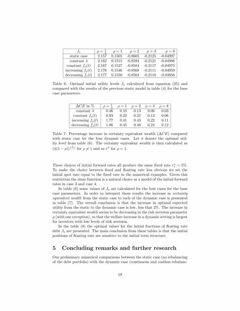
Table 6: Optimal initial utility levels Js calculated from equation (25) andcompared with the results of the previous static model in table (4) for the basecase parameters.

∆CE in % ρ = 12 ρ = 1 ρ = 2 ρ = 4 ρ = 8

constant λ 0.46 0.10 0.13 0.06 0.03constant fs(t) 0.93 0.22 0.24 0.13 0.06increasing fs(t) 1.77 0.41 0.43 0.22 0.11decreasing fs(t) 1.86 0.45 0.48 0.24 0.12

Table 7: Percentage increase in certainty equivalent wealth (∆CE) comparedwith static case for the four dynamic cases. Let u denote the optimal util-ity level from table (6). The certainty equivalent wealth is then calculated as(u(1− ρ))

11−ρ for ρ 6= 1 and as eu for ρ = 1.

These choices of initial forward rates all produce the same fixed rate rxs = 5%.

To make the choice between fixed and floating rate less obvious we set theinitial spot rate equal to the fixed rate in the numerical examples. Given thisrestriction the sinus function is a natural choice as a model of the initial forwardrates in case 3 and case 4.

In table (6) some values of Js are calculated for the four cases for the basecase parameters. In order to interpret these results the increase in certaintyequivalent wealth from the static case to each of the dynamic case is presentedin table (7). The overall conclusion is that the increase in optimal expectedutility from the static to the dynamic case is low, less that 2%. The increase incertainty equivalent wealth seems to be decreasing in the risk aversion parameterρ (with one exception), so that the welfare increase in a dynamic setting is largestfor investors with low levels of risk aversion.

In the table (8) the optimal values for the initial fractions of floating ratedebt βs are presented. The main conclusion from these tables is that the initialpositions of floating rate are sensitive to the initial term structure.

5 Concluding remarks and further research

Our preliminary numerical comparisons between the static case (no rebalancingof the debt portfolio) with the dynamic case (continuous and costless rebalanc-

19

βs ρ = 12 ρ = 1 ρ = 2 ρ = 4 ρ = 8

static case 1.231 0.6187 0.3100 0.1551 0.07759constant λ 0.2320 0.1160 0.05800 0.0290 0.0145

constant fs(t) -0.4478 -0.2239 -0.1120 -0.05598 -0.02799increasing fs(t) 1.7119 0.8602 0.4298 0.2150 0.1075decreasing fs(t) -2.615 -1.308 -0.6536 -0.3668 -0.1635

Table 8: Optimal initial fractions of floating rate debt βs calculated from theresult in proposition 6 and compared with the results of the previous staticmodel in table (5) for the base case parameters.

ing) indicate, perhaps surprisingly, low increase in ’welfare’ in dynamic situationcompared to static situation. At least this is the case for high levels of relativerisk aversion.

In the dynamic case the optimal initial fractions of floating rate debt arepartly determined by the initial forward interest rates, which do not influencethe corresponding optimal fraction in the static case. Therefore, we do notlearn anything about the optimal floating rate debt fraction in the dynamiccase from the static case. Even if we are willing to assume that the marketprice of interest rate risk is constant the initial optimal fractions of floating ratedebt are different in the static and dynamic cases.

The research in this article can be extended in a number of ways. First,realism can be improved by introducing a multi-factor interest rate model. Also,transaction costs can be introduced, in the spirit of Davis and Norman (1990),Korn (1998), Øksendal and Sulem (2000), and Zakamouline (2002) in order tomake the set-up closer to real world situations. Finally, this set-up may be usedto study the effect of a stochastic collateral (W ).

A Appendix

In this appendix a number of detailed calculations is collected.From equation (2) direct calculations give∫ T

t

λsds =q

v

[(m− rx

t )(T − t) +1q(rt − ft(T ))

]−

q

v

[v2

4q3(2q(T − t)− 1 + e−2q(T−t))

](32)

and∫ T

t

λseqsds =

q

veqT

[m

q(1− e−q(T−t))− 1

q(ft(T )− rte

−q(T−t))]

+

q

veqT

[v2

2q3(2e−q(T−t) − e−2q(T−t) − 1)

]. (33)

20

From the equations (2) and (4) by using (32) and (33) it follows that

Cov

(∫ T

s

rtdt,

∫ T

s

λs(t)dBt|Fs

)=

(rs −m)1− e−q(T−s)

q+ (m− rx

s )(T − s)− 12σ2

s,T . (34)

It is now straight forward to calculate

V 2s,T = Var

(∫ T

s

rtdt +∫ T

s

λs(t)dBt|Fs

)

= σ2s,T +

∫ T

s

λs(t)2dt + 2Cov

(∫ T

s

rtdt,

∫ T

s

λs(t)dBt|Fs

)

=∫ T

s

λs(t)2dt + 2[(rs −m)

1− e−q(T−s)

q+ (m− rx

s )(T − s)]

. (35)

The partial derivative of V 2s,T is

∂V 2s,T

∂s= −[λs(t)2 + 2[(rs −m)e−q(T−s) + m− rx

s ]]. (36)

In the case where λ is constant we obtain from equation (4)

Cov

(∫ T

s

rtdt,

∫ T

s

λdBt|Fs

)= µs,T − 1

2σ2

s,T − rxs (T − s). (37)

and

V 2s,T = Var

(∫ T

s

rtdt +∫ T

s

λdBt|Fs

)= λ2(T − s)+ 2(µs,T − rx

s (T − s)). (38)

References

I. Bajeux-Besnainou, J. W. Jordan, and R. Portait. An asset allocation puzzle:Comment. American Economic Review, 91:1170—1179, 2001.

M. J. Brennan and Y. Xia. Stochastic interest rates and the bond-stock mix.European Finance Review, 4:197—210, 2000.

J. Y. Cambell and J. F. Cocco. Houshold risk management and optimal mort-gage choice. Working-paper, Harvard University, 2002.

N. Canner, N. G. Mankiw, and D. N. Weil. An asset allocation puzzle. AmericanEconomic Review, 87:181—191, 1997.

21

K. C. Chan, G. A. Karolyi, F. A. Longstaff, and A. B. Sanders. An empiricalcomparison of alternative models of the short-term interest rate. The Journalof Finance, XLVII(3):1209–1227, July 1992.

J. C. Cox and C.-F. Huang. Optimal consumption and portfolio policies whenasset prices follow a diffusion process. Journal of Economic Theory, 49:33—83, 1989.

M. Davis and A. Norman. Portfolio selection with transaction costs. Mathe-matics of Operations Research, 15(4):676—713, 1990.

L. Eeckhoudt and C. Gollier. Risk — evaluation, management and sharing.Harvester Wheatsheaf, New York, USA, 1995.

D. Heath, R. Jarrow, and A. J. Morton. Bond pricing and the term struc-ture of interest rates: A new methodology for contingent claims valuation.Econometrica, 60(1):77–105, Jan. 1992.

C.-f. Huang and R. H. Litzenberger. Foundations for Financial Economics.North-Holland Publishing Company, New York, New York, USA, 1988.

J. Hull and A. White. Pricing interest rate derivative securities. The Review ofFinancial Studies, 3(4):573–592, 1990.

R. Korn. Portfolio optimisation with strictly positive transaction costs andimpulse control. Finance and Stochastics, 2:85—114, 1998.

R. C. Merton. Lifetime portfolio selection under uncertainty: The continuous-time case. Review of Economics and Statistics, 51:247—257, 1969.

R. C. Merton. Optimum consumption and portfolio rules in a continuous timemodel. Journal of Economic Theory, 3:373–413, Dec. 1971. Erratum: Merton(1973). Reprinted in (Merton, 1990, Chapter 5).

R. C. Merton. Erratum. Journal of Economic Theory, 6:213–214, 1973.

R. C. Merton. Continuous-Time Finance. Basil Blackwell Inc., Padstow, GreatBritain, 1990.

K. R. Miltersen and S.-A. Persson. Pricing rate of return guarantees in a heath-jarrow-morton framework. Insurance: Mathematics and Economics, 25:307–325, 1999.

J. Mossin. Aspects of rational insurance purchasing. Journal of Political Econ-omy, 76:553—568, 1968.

C. Munk and C. Sørensen. Optimal consumption and investment strategies withstochastic interest rates. Working-paper, Odense University, Denmark, 2001.

B. Øksendal and A. Sulem. Optimal consumption and portfolio with bothfixed and proportional transaction costs. Working-paper, University of Oslo,Norway, 2000.

22

S. Pliska. A stochastic calculus model of continuous trading: Optimal portfolios.Mathematics of Operations Research, 11:371—382, 1986.

C. Sørensen. Dynamic asset allocation and fixed income management. Journalof Financial and Quantitative Analysis, 34:513—531, 1999.

O. Vasicek. An equilibrium characterization of the term structure. Journal ofFinancial Economics, 5:177–188, 1977.

V. I. Zakamouline. Optimal portfolio selection with both fixed and proportionaltransaction costs for a crra investor with finite horizon. Working-paper, Nor-wegian School of Economics and Business Administration, 2002.

23