Derivation and Validation of Metrics for Breast Cancer

Diagnosis from Diffuse Optical Tomography Imaging Data

Derivation and Validation of Metrics for Breast Cancer

Diagnosis from Diffuse Optical Tomography Imaging Data

Randall L. Barbour, Ph.D.

SUNY Downstate Medical CenterBrooklyn, New York

2

Corrosion Cast of Tumor Vasculature. ‘tp’, = tumor periphery, ‘st’ = surrounding tissue. (M. Molls and P. Vaupel, Eds. Blood Perfusion and Microenvironment of Human Tumors: Implications for Clinical Radiooncology. Springer-Verlag, New York 2000.)

Corrosion Cast of Tumor Vasculature

3

Basic Features of Tumor Vasculature

• Leaky vessels – Increased interstitial pressure

• Poorly developed vessels– altered/absence of normal control mechanisms

• Relative state of hypoxemia

• Dynamic optical studies should prove sensitive to multiple features of tumor biology.

4

Motivation For Dynamic Studies

• Functional Parameters Associated with Blood Delivery to Tissue– Tissue Oxygen Demand– Vascular Compliance– Autoregulation (e.g., reactive hyperemia)– Autonomic Control (modulation of blood delivery)

– Varying metabolic demand influences tissue-vascular coupling• Response to provocation• Influence of disease• Effects of drugs

– Technical Benefits • Multiple features• High intrinsic contrast• No need for injection

• Why Optical?– Simultaneous assessment of metabolic demand and vascular dynamics.

5

Dual Breast Imaging Result

-4.0E-05

-2.0E-05

0.0E+00

2.0E-05

4.0E-05

6.0E-05

8.0E-05

1.0E-04

1.2E-04

1.4E-04

2500 2550 2600 2650 2700 2750 2800 2850 2900 2950 3000

Imaging Frames

Estim

ate

d

D Hb

red

[m

ol/l]

1 2 3 4 5 6 7

1.5e-8

0

-9.3e-9

2.1e-8

0

-1.2e-8

Left

(tum

or)

1 2 3 4 5 6 7Rig

ht (

heal

thy)

D H

bred

[m

ol/l]

Imaging frames

6

Strategies for Data Analysis

Large dimensional

data sets.

Time Series Measures

Inherently information rich

To Obtain Useful Information: Consider the big picture

7

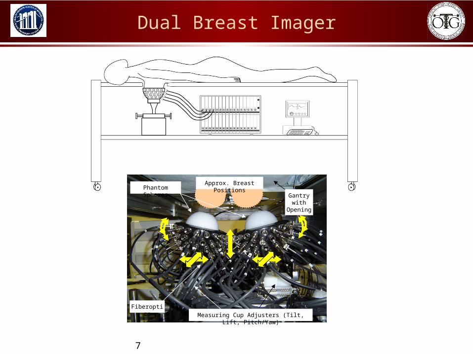
Dual Breast Imager

Phantom SpheresGantry

withOpening

Fiberoptics

Measuring Cup Adjusters (Tilt, Lift, Pitch/Yaw)

Approx. Breast Positions

8

Instrumentation

11a 11b

10a 10b

9b9a

6b6a

8Power Supply

Motor Controller

(4,5)b(4,5)a

12

11a 11b

10a 10b

9b9a

6b6a

8Power Supply

Motor Controller

(4,5)b(4,5)a

12

6a 6b

(4,5)a (4,5)b

9a 9b12

10a 10b

11a 11b

8

11a 11b

10a 10b

9b9a

6b6a

8Power Supply

Motor Controller

(4,5)b(4,5)a

12

Power Supply

Motor Controller

Detection Unit

Stepper Motor Controller

PC

Fiber optic

s

Measuring Heads

Support rods

Adjustable arcsStrain

reliefes

Steppermotors

Support rods

Adjustable arcsStrain

reliefes

Steppermotors

9

Approach

• Simple Idea:

– Define utility of scalar metrics of amplitude, variance and spatial coordination of low frequency hemodynamics obtained from baseline measures

– Amplitude response to a simple provocation

– Simultaneous Measures: Paired difference

10

Power Spectrum of Hb Signal

0 0.1 0.2 0.3 0.4 0.5 0.6 0.7 0.8 0.9-3

-2

-1

0

1

2

3

4

5

6x 10

-9

Frequency (Hz)

Gro

up

-ave

rag

e In

ter-

bre

ast A

mp

litu

de

Diff

ere

nce

Spatial Mean Result, Hbtotal

Cancer Healthy

11

Dimension Reduction: Temporal Spatial Averaging

Time

Position (IV)

Spatial map of temporal standard

deviation (SD)

(III)Baseline temporal mean is 0, by

definition

temporal integration

drop position information

sorted parameter value

100

0

Hbdeoxy

Hboxy

(II)

spatial integration

mean SD

scalar quantities

(I)

12

Spatial Temporal Averaging

Time

Position (IV)

spatial integration

(II)

(I)

Time series of spatial mean → O2 demand / metabolic responsiveness

Time series of spatial SD → Spatial heterogeneity

temporal integration

Temporal mean of spatial mean time series: 0, by definition

Temporal SD of spatial mean time series

Temporal mean of spatial SD time series

Temporal SD of spatial SD time series

scalar quantities

13

1. Starting point is reconstructed image time series (IV)

2. Use (complex Morlet) wavelet transform as a time-domain bandpass filter operation

A. Output is an image time series (IV) of amplitude vs. time vs. spatial position, for the frequency band of interest

B. Filtered time series can be obtained for more than one frequency band

3. Recompute previously considered, but starting with the wavelet amplitude time series

Method 2: Time-frequency (wavelet) analysis

time

f1

f2

14

Vasomotor Coordination

Time (s)

FE

M m

esh

no

de

100 200 300 400 500 600 700

0

500

1000

1500

2000

0.5

1

1.5

2

2.5

Time (s)

FE

M m

esh

no

de

100 200 300 400 500 600 700

0

500

1000

1500

2000

0.5

1

1.5

2

2.5

Healthy Breast Tumor Breast

15

Method 3: Provocation Analysis: Healthy Subject

Left breast (blue curve) and right breast (red curve)

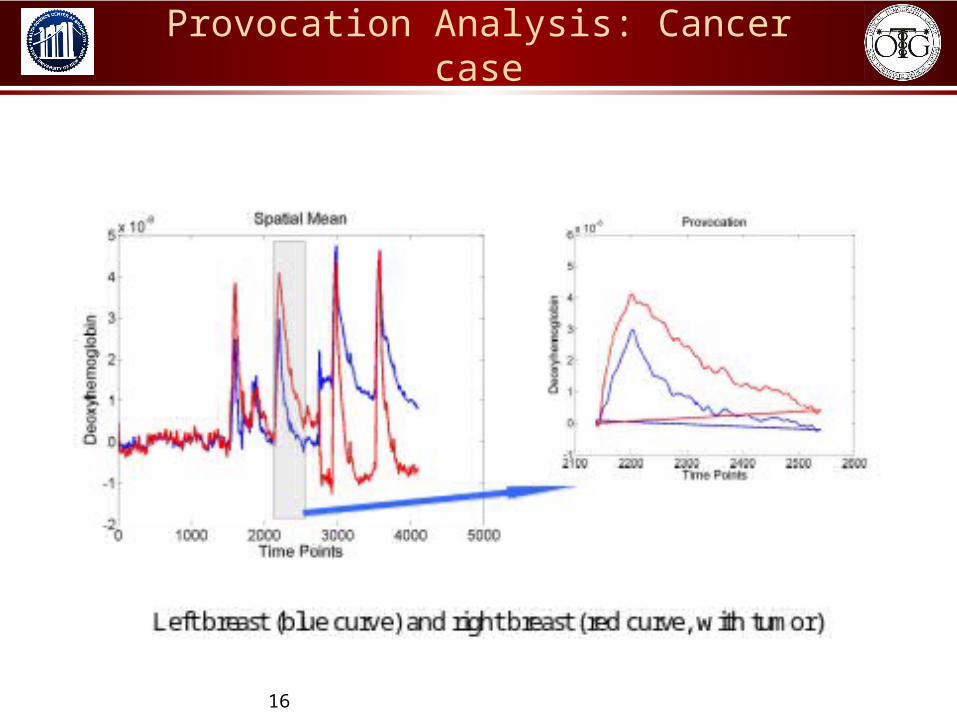
16

Provocation Analysis: Cancer case

17

Scalar Metrics Explored

ExperimentalCondition

Tumor-AssociatedPhenotype

Scalar Metric

Re

sting

Sta

te

Hypoxia

SpatialCoordination

EvokedResponse

Angiogenesis

2

22. , t vt

SSDTSD x t N SMTSD N rr

23. , , v v tt

TMSSD x t x t N N N r rr r

24. , v tt

TSDSM x t N N rr

22

5. , , v v ttTSDSSD x t x t N N TMSSD N r r

r r

2

, , , ,

, , ,

6. 100 , , , ,

where:

, , , (Complex Morlet wavelet decomposition),

(Normalize to unit mean value, in, , , , , ,

the frequency bands of inter

l h t l h l h t l ht t t

l h t l h l ht

SC f N u t f u t f N u t f

x t M t f

U t f N M t f M t f

r r

r r r

, ,

,est)

, , , (Average over the image volume).l h l h vu t f U t f N rr

2

1

2 1 2 1 1 2 2 1 2 17.t

t

A y t y t y t t t y t t y t t t t t

1 21 2

8. max mint t tt t t

R y t y t

21. , t vt

SMTSD x t N N rr

18

Subject Population

Subject Group Breast Pathology Status NAge (yr)

[mean ± SD]BMI (kg-m2)[mean ± SD]

Tumor Size[largest dimension]

Clinical Description

Retrospective

Active CA 14 47.9 ± 12.3 28.7 ± 5.310 ≤ 3 cm4 > 3 cm

10 ductal carcinoma1 ductal & lobular carcinoma

1 mucinous carcinoma1 metastatic CA

1 inflammatory CA

Prior CA 3 50.7 ± 9.4 30.4 ± 0.5 —All had lumpectomies 2-3 yr

prior to NIRS study

Pre-CA 0 — — — —

Non-CA Pathology 11 45.7 ± 5.628.7 ± 5.5

(N = 7)—

3 fibrocystic disease4 breast cyst

1 axillary cyst2 benign breast lumps

1 breast reduction surgery

No Historyof Breast Pathology

9 41.6 ± 10.0 30.3 ± 7.2 — —

19

Subject Population

Prospective

Active CA 14 51.4 ± 10.9 30.4 ± 4.55 ≤ 3 cm9 > 3 cm(a

13 ductal carcinoma1 axillary adenocarcinoma with

mammary duct ectasiaand hyperplasia

Prior CA 4 60.8 ± 9.3 25.5 ± 1.7 —

3 prior ductal carcinoma1 prior mucinous carcinomaAll had lumpectomies 2-6 yr

prior to NIRS study

Pre-CA 4 53.5 ± 3.429.0 ± 4.1

(N = 3)—

2 DCIS1 atypical ductal hyperplasia

1 extremely dense breasts

Non-CA Pathology 6 43.7 ± 8.426.6 ± 4.9

(N = 4)—

1 cystic disease2 fibrocystic changes

1 fibrosis1 benign breast lump

1 breast reduction surgery

No Historyof Breast Pathology

8 44.0 ± 6.8 30.5 ± 8.9 — —

20

Patient Demographics

Age (years) BMI (kg-m-2) n1 Mean SD Range n2 Mean SD Range

(1) Retrospective / Training Group

14 47.9 12.3 29-70 14 28.7 5.3 21.6-43.9 Cancer (CA)

Subjects (2) Prospective / Validation Group

14 51.4 10.9 37-71 14 30.4 4.5 22.7-38.1

(3) Retrospective / Training Group

23 44.7 8.6 26-62 19(b 30.1 6.1 18.4-44.4 Non-CA Subjects (4) Prospective /

Validation Group 22(a 48.7 10.0 30-69 18(b 28.2 6.6 21.2-48.5

p-value(a

Comparison Age BMI

(1) vs. (3) 0.39 0.51 (2) vs. (4) 0.47 0.33 (1) vs. (2) 0.45 0.38 (3) vs. (4) 0.17 0.40

21

Logistic Regression Applied

Metrics

Pro

babi

lity

Metrics calculated and selected based on t-tests & ROC curves

Metrics used as inputs into logistic regression model

Logistic regression model calculates i for each metric (Xi)

Using i, a predicted probability distribution can be created

New patient’s Xi used to generate probability of cancer in patient

X1 = .43; X2 = -.05New Patient’s Values

Linear Model: P(cancer) = 0.75

Logistic Regression: P(cancer) = 0.90

22

Scalar Metrics Examined

Hypothesis Driven

Metrics Data Driven

Metrics Data Categories

1 1 2 3 1,2 1,2 1,2 1,2 1,3 2,3 2,3 1,2,3 1,2,3 1 2 3 3 1,2 1,2 2,3 1, [3]

1,2, [3]

Multiparameter Metric

Scalar Parameters

1 2 3 4 5 6 7 8 9 10 11 12 13 14 15 16 17 18 19 20 21 22

SMTSDoxy X X X X SSDTSDoxy X X X X X TMSSDoxy X X X X X X X TSDSMoxy TSDSSDoxy X X SMTSDdeoxy X X X SSDTSDdeoxy X X X TMSSDdeoxy X X X TSDSMdeoxy X X X X X X TSDSSDdeoxy X X X X X SMTSDtot X X X X X SSDTSDtot X X TMSSDtot X X X X X TSDSMtot X X

Hyp

oxia

(1

)

TSDSSDtot X X WLoxy X X X X X X

WHoxy

WLdeoxy X X X X X X X X

Syn

chro

ny(2

)

WHdeoxy X X X X X X X X X

VMAoxy X X

VMAdeoxy X

VMRoxy X X X X X X X

Para

met

er C

ateg

ory

Ang

ioge

nesi

s (3

)

VMRdeoxy X X X X X

23

Multivariate Predictor Performance

Multivariate Predictor 1 2 3 4 5 6 7 8 9 10 11 12 13 14 15 16 17 18 19 20 21 22

R 85.7 90 90 80 80 78.6 64.3 71.4 85.7 100 80 80 50 50 57.1 90 80 78 100 90 80 80 Sn

P 57.1 57.1 64.3 78.6 71.4 64.3 78.6 57.1 78.6 78.6 71.4 71.4 85.7 64.3 57.1 71.4 71.4 85.7 78.6 57.1 64.3 71.4 R 95 81.8 90.9 90.9 100 90 95 90 95 90 90.9 90.9 90 80 95 90.9 90.9 80 95 90.9 81.8 90.9

Sp P 86.7 84.6 76.9 92.3 92.3 60 86.7 93.3 100 100 84.6 92.3 93.3 93.3 100 84.6 84.6 100 93.3 61.5 84.6 69.2

24

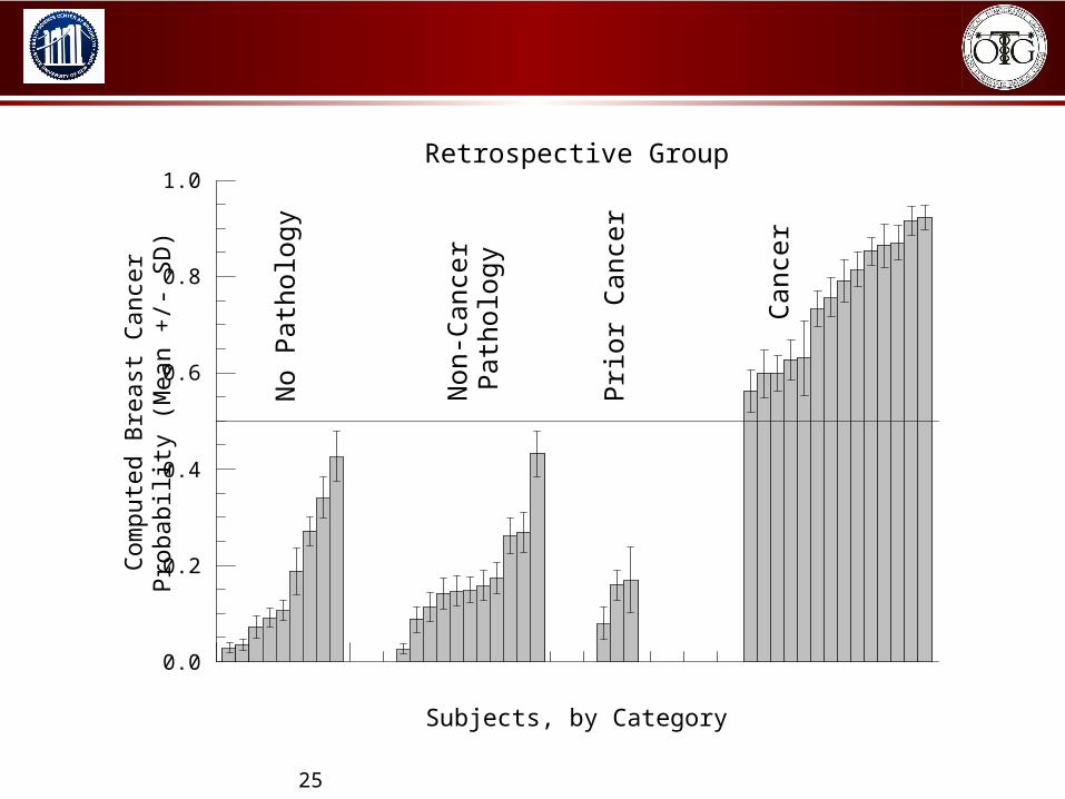
Performance of Multivariate Predictor Averages

Retrospective Group

Sensitivity (%) Specificity (%)

Per

cent

age

of P

redi

ctor

Agg

rega

tes

4050

6070

8090

4050

6070

8090

0

5

10

15

20

25

Sensitivity (%)Specificity (%)

Perc

enta

ge o

f Pr

edic

tor A

ggre

gate

s

4050

6070

8090

4050

6070

8090

0

5

10

15

20

25

(Two views of the same histogram.)

(This one has the same orientation as the ones in Figures 2 and 3.)

(This one is rotated 90°, so that all the bars are visible.)

25

No

Path

olog

y

Non

-Can

cer

Path

olog

y

Prio

r C

ance

r

Can

cer

Subjects, by Category

0 10 20 30 40 50

Com

pute

d B

reas

t Can

cer

Pro

babi

lity

(Mea

n +

/- S

D)

0.0

0.2

0.4

0.6

0.8

1.0Retrospective Group

26C

ance

r

Pre

-Can

cer

Pri

or C

ance

r

Non

-Can

cer

Pat

holo

gy

No

Pat

holo

gy

Subjects, by Category

0 10 20 30 40 50

Com

pute

d B

reas

t Can

cer

Pro

babi

lity

(Mea

n +

/- S

D)

0.0

0.2

0.4

0.6

0.8

1.0Prospective Group

27

Summary:

• The amplitude and spatial coordination of the Hb signal is notable altered in tumor bearing breasts.

• Multivariate metrics derived from simple scalar quantities derived from resting and provoked responses yield predictors having high discriminatory values.