description - data analysis and statistical software | stata stata.com functions — functions...
TRANSCRIPT
Title stata.com
functions — Functions
Description Acknowledgments References Also see
DescriptionThis entry describes the functions allowed by Stata. For information on Mata functions, see
[M-4] intro.
A quick note about missing values: Stata denotes a numeric missing value by ., .a, .b, . . . ,or .z. A string missing value is denoted by "" (the empty string). Here any one of these may bereferred to by missing. If a numeric value x is missing, then x ≥ . is true. If a numeric value x isnot missing, then x < . is true.
Functions are listed under the following headings:
Mathematical functionsProbability distributions and density functionsRandom-number functionsString functionsProgramming functionsDate and time functionsSelecting time spansMatrix functions returning a matrixMatrix functions returning a scalar
Mathematical functions
abs(x)Domain: −8e+307 to 8e+307Range: 0 to 8e+307Description: returns the absolute value of x.
acos(x)Domain: −1 to 1Range: 0 to πDescription: returns the radian value of the arccosine of x.
acosh(x)Domain: 1 to 8.9e+307Range: 0 to 709.77Description: returns the inverse hyperbolic cosine of x, acosh(x) = ln(x+
√x2 − 1).
asin(x)Domain: −1 to 1Range: −π/2 to π/2Description: returns the radian value of the arcsine of x.
asinh(x)Domain: −8.9e+307 to 8.9e+307Range: −709.77 to 709.77Description: returns the inverse hyperbolic sine of x, asinh(x) = ln(x+
√x2 + 1).
1
2 functions — Functions
atan(x)Domain: −8e+307 to 8e+307Range: −π/2 to π/2Description: returns the radian value of the arctangent of x.
atan2(y, x)Domain y: −8e+307 to 8e+307Domain x: −8e+307 to 8e+307Range: −π to πDescription: returns the radian value of the arctangent of y/x, where the signs of the parameters
y and x are used to determine the quadrant of the answer.
atanh(x)Domain: −1 to 1Range: −8e+307 to 8e+307Description: returns the inverse hyperbolic tangent of x, atanh(x) = 1
2{ln(1 +x)− ln(1−x)}.
ceil(x)Domain: −8e+307 to 8e+307Range: integers in −8e+307 to 8e+307Description: returns the unique integer n such that n− 1 < x ≤ n.
returns x (not “.”) if x is missing, meaning that ceil(.a) = .a.
Also see floor(x), int(x), and round(x).
cloglog(x)Domain: 0 to 1Range: −8e+307 to 8e+307Description: returns the complementary log-log of x,
cloglog(x) = ln{−ln(1− x)}.
comb(n,k)Domain n: integers 1 to 1e+305Domain k: integers 0 to nRange: 0 to 8e+307 and missingDescription: returns the combinatorial function n!/{k!(n− k)!}.
cos(x)Domain: −1e+18 to 1e+18Range: −1 to 1Description: returns the cosine of x, where x is in radians.
cosh(x)Domain: −709 to 709Range: 1 to 4.11e+307Description: returns the hyperbolic cosine of x, cosh(x) = {exp(x) + exp(−x)}/2.
digamma(x)Domain: −1e+15 to 8e+307Range: −8e+307 to 8e+307 and missingDescription: returns the digamma() function, d lnΓ(x)/dx. This is the derivative of lngamma(x).
The digamma(x) function is sometimes called the psi function, ψ(x).
functions — Functions 3
exp(x)Domain: −8e+307 to 709Range: 0 to 8e+307Description: returns the exponential function ex. This function is the inverse of ln(x).
floor(x)Domain: −8e+307 to 8e+307Range: integers in −8e+307 to 8e+307Description: returns the unique integer n such that n ≤ x < n+ 1.
returns x (not “.”) if x is missing, meaning that floor(.a) = .a.
Also see ceil(x), int(x), and round(x).
int(x)Domain: −8e+307 to 8e+307Range: integers in −8e+307 to 8e+307Description: returns the integer obtained by truncating x toward 0; thus,
int(5.2) = 5int(-5.8) = −5
returns x (not “.”) if x is missing, meaning that int(.a) = .a.
One way to obtain the closest integer to x is int(x+sign(x)/2), whichsimplifies to int(x+0.5) for x ≥ 0. However, use of the round() function ispreferred. Also see ceil(x), int(x), and round(x).
invcloglog(x)Domain: −8e+307 to 8e+307Range: 0 to 1 and missingDescription: returns the inverse of the complementary log-log function of x,
invcloglog(x) = 1− exp{−exp(x)}.
invlogit(x)Domain: −8e+307 to 8e+307Range: 0 to 1 and missingDescription: returns the inverse of the logit function of x,
invlogit(x) = exp(x)/{1 + exp(x)}.
ln(x)Domain: 1e–323 to 8e+307Range: −744 to 709Description: returns the natural logarithm, ln(x). This function is the inverse of exp(x).
The logarithm of x in base b can be calculated via logb(x) = loga(x)/ loga(b).Hence,
log5(x) = ln(x)/ln(5) = log(x)/log(5) = log10(x)/log10(5)log2(x) = ln(x)/ln(2) = log(x)/log(2) = log10(x)/log10(2)
You can calculate logb(x) by using the formula that best suits your needs.
4 functions — Functions
lnfactorial(n)Domain: integers 0 to 1e+305Range: 0 to 8e+307Description: returns the natural log of factorial = ln(n!).
To calculate n!, use round(exp(lnfactorial(n)),1) to ensure that the result isan integer. Logs of factorials are generally more useful than the factorials themselvesbecause of overflow problems.
lngamma(x)Domain: −2,147,483,648 to 1e+305 (excluding negative integers)Range: −8e+307 to 8e+307Description: returns ln{Γ(x)}. Here the gamma function, Γ(x), is defined by
Γ(x) =∫∞0tx−1e−tdt. For integer values of x > 0, this is ln((x− 1)!).
lngamma(x) for x < 0 returns a number such that exp(lngamma(x)) is equal tothe absolute value of the gamma function, Γ(x). That is, lngamma(x) always returnsa real (not complex) result.
log(x)Domain: 1e–323 to 8e+307Range: −744 to 709Description: returns the natural logarithm, ln(x), which is a synonym for ln(x). Also see ln(x)
for more information.
log10(x)Domain: 1e–323 to 8e+307Range: −323 to 308Description: returns the base-10 logarithm of x.
logit(x)Domain: 0 to 1 (exclusive)Range: −8e+307 to 8e+307 and missingDescription: returns the log of the odds ratio of x,
logit(x) = ln {x/(1− x)}.
max(x1,x2,. . .,xn)Domain x1: −8e+307 to 8e+307 and missingDomain x2: −8e+307 to 8e+307 and missing. . .Domain xn: −8e+307 to 8e+307 and missingRange: −8e+307 to 8e+307 and missingDescription: returns the maximum value of x1, x2, . . . , xn. Unless all arguments are missing,
missing values are ignored.max(2,10,.,7) = 10max(.,.,.) = .

functions — Functions 5
min(x1,x2,. . .,xn)Domain x1: −8e+307 to 8e+307 and missingDomain x2: −8e+307 to 8e+307 and missing. . .Domain xn: −8e+307 to 8e+307 and missingRange: −8e+307 to 8e+307 and missingDescription: returns the minimum value of x1, x2, . . . , xn. Unless all arguments are missing,
missing values are ignored.min(2,10,.,7) = 2min(.,.,.) = .
mod(x,y)Domain x: −8e+307 to 8e+307Domain y: 0 to 8e+307Range: 0 to 8e+307Description: returns the modulus of x with respect to y.
mod(x, y) = x− y floor(x/y)mod(x,0) = .
reldif(x,y)Domain x: −8e+307 to 8e+307 and missingDomain y: −8e+307 to 8e+307 and missingRange: −8e+307 to 8e+307 and missingDescription: returns the “relative” difference |x− y|/(|y|+ 1).
returns 0 if both arguments are the same type of extended missing value.returns missing if only one argument is missing or if the two arguments are
two different types of missing.
round(x,y) or round(x)Domain x: −8e+307 to 8e+307Domain y: −8e+307 to 8e+307Range: −8e+307 to 8e+307Description: returns x rounded in units of y or x rounded to the nearest integer if the argument
y is omitted.returns x (not “.”) if x is missing, meaning that round(.a) = .a and
round(.a,y) = .a if y is not missing; if y is missing, then “.” is returned.
For y = 1, or with y omitted, this amounts to the closest integer to x; round(5.2,1)is 5, as is round(4.8,1); round(-5.2,1) is −5, as is round(-4.8,1). Therounding definition is generalized for y 6= 1. With y = 0.01, for instance, x isrounded to two decimal places; round(sqrt(2),.01) is 1.41. y may also be largerthan 1; round(28,5) is 30, which is 28 rounded to the closest multiple of 5.For y = 0, the function is defined as returning x unmodified. Also seeint(x), ceil(x), and floor(x).
sign(x)Domain: −8e+307 to 8e+307 and missingRange: −1, 0, 1 and missingDescription: returns the sign of x: −1 if x < 0, 0 if x = 0, 1 if x > 0, and missing
if x is missing.
6 functions — Functions
sin(x)Domain: −1e+18 to 1e+18Range: −1 to 1Description: returns the sine of x, where x is in radians.
sinh(x)Domain: −709 to 709Range: −4.11e+307 to 4.11e+307Description: returns the hyperbolic sine of x, sinh(x) = {exp(x)− exp(−x)}/2.
sqrt(x)Domain: 0 to 8e+307Range: 0 to 1e+154Description: returns the square root of x.
sum(x)Domain: all real numbers and missingRange: −8e+307 to 8e+307 (excluding missing)Description: returns the running sum of x, treating missing values as zero.
For example, following the command generate y=sum(x), the jth observationon y contains the sum of the first through jth observations on x. See [D] egen foran alternative sum function, total(), that produces a constant equal to the overallsum.
tan(x)Domain: −1e+18 to 1e+18Range: −1e+17 to 1e+17 and missingDescription: returns the tangent of x, where x is in radians.
tanh(x)Domain: −8e+307 to 8e+307Range: −1 to 1 and missingDescription: returns the hyperbolic tangent of x,
tanh(x) = {exp(x)− exp(−x)}/{exp(x) + exp(−x)}.
trigamma(x)Domain: −1e+15 to 8e+307Range: 0 to 8e+307 and missingDescription: returns the second derivative of lngamma(x) = d2 lnΓ(x)/dx2. The trigamma()
function is the derivative of digammma(x).
trunc(x) is a synonym for int(x).
Technical note
The trigonometric functions are defined in terms of radians. There are 2π radians in a circle. Ifyou prefer to think in terms of degrees, because there are also 360 degrees in a circle, you mayconvert degrees into radians by using the formula r = dπ/180, where d represents degrees and rrepresents radians. Stata includes the built-in constant pi, equal to π to machine precision. Thus,to calculate the sine of theta, where theta is measured in degrees, you could type
sin(theta* pi/180)
functions — Functions 7
atan() similarly returns radians, not degrees. The arccotangent can be obtained as
acot(x) = pi/2 - atan(x)
Probability distributions and density functions
The probability distributions and density functions are organized under the following headings:
Beta and noncentral beta distributionsBinomial distributionChi-squared and noncentral chi-squared distributionsDunnett’s multiple range distributionF and noncentral F distributionsGamma distributionHypergeometric distributionNegative binomial distributionNormal (Gaussian), log of the normal, and binormal distributionsPoisson distributionStudent’s t and noncentral Student’s t distributionsTukey’s Studentized range distribution
Beta and noncentral beta distributions
ibeta(a,b,x)Domain a: 1e–10 to 1e+17Domain b: 1e–10 to 1e+17Domain x: −8e+307 to 8e+307
Interesting domain is 0 ≤ x ≤ 1Range: 0 to 1Description: returns the cumulative beta distribution with shape parameters a and b defined by
Ix(a, b) =Γ(a+ b)
Γ(a)Γ(b)
∫ x
0
ta−1(1− t)b−1 dt
returns 0 if x < 0.returns 1 if x > 1.
ibeta() returns the regularized incomplete beta function, also known as theincomplete beta function ratio. The incomplete beta function withoutregularization is given by (gamma(a)*gamma(b)/gamma(a+b))*ibeta(a,b,x)or, better when a or b might be large,exp(lngamma(a)+lngamma(b)-lngamma(a+b))*ibeta(a,b,x).
Here is an example of the use of the regularized incomplete beta function.Although Stata has a cumulative binomial function (see binomial()), theprobability that an event occurs k or fewer times in n trials, when theprobability of one event is p, can be evaluated ascond(k==n,1,1-ibeta(k+1,n-k,p)). The reverse cumulative binomial(the probability that an event occurs k or more times) can be evaluatedas cond(k==0,1,ibeta(k,n-k+1,p)). See Press et al. (2007, 270–273)for a more complete description and for suggested uses for this function.
8 functions — Functions
betaden(a,b,x)Domain a: 1e–323 to 8e+307Domain b: 1e–323 to 8e+307Domain x: −8e+307 to 8e+307
Interesting domain is 0 ≤ x ≤ 1Range: 0 to 8e+307Description: returns the probability density of the beta distribution,
betaden(a,b,x) =xa−1(1− x)b−1∫∞
0ta−1(1− t)b−1dt
=Γ(a+ b)
Γ(a)Γ(b)xa−1(1− x)b−1
where a and b are the shape parameters.returns 0 if x < 0 or x > 1.
ibetatail(a,b,x)Domain a: 1e–10 to 1e+17Domain b: 1e–10 to 1e+17Domain x: −8e+307 to 8e+307
Interesting domain is 0 ≤ x ≤ 1Range: 0 to 1Description: returns the reverse cumulative (upper tail or survivor) beta distribution with shape
parameters a and b defined by
ibetatail(a,b,x) = 1− ibeta(a,b,x) =
∫ 1
x
betaden(a,b,t) dt
returns 1 if x < 0.returns 0 if x > 1.
ibetatail() is also known as the complement to the incomplete beta function(ratio).
invibeta(a,b,p)Domain a: 1e–10 to 1e+17Domain b: 1e–10 to 1e+17Domain p: 0 to 1Range: 0 to 1Description: returns the inverse cumulative beta distribution: if ibeta(a,b,x) = p,
then invibeta(a,b,p) = x.
invibetatail(a,b,p)Domain a: 1e–10 to 1e+17Domain b: 1e–10 to 1e+17Domain p: 0 to 1Range: 0 to 1Description: returns the inverse reverse cumulative (upper tail or survivor) beta distribution:
if ibetatail(a,b,x) = p, then invibetatail(a,b,p) = x.
functions — Functions 9
nibeta(a,b,np,x)Domain a: 1e–323 to 8e+307Domain b: 1e–323 to 8e+307Domain np: 0 to 10,000Domain x: −8e+307 to 8e+307
Interesting domain is 0 ≤ x ≤ 1Range: 0 to 1Description: returns the cumulative noncentral beta distribution
Ix(a, b, np) =
∞∑j=0
e−np/2(np/2)j
Γ(j + 1)Ix(a+ j, b)
where a and b are shape parameters, np is the noncentrality parameter, x is thevalue of a beta random variable, and Ix(a, b) is the cumulative beta distribution,ibeta().
returns 0 if x < 0.returns 1 if x > 1.
nibeta(a,b,0,x)= ibeta(a,b,x), but ibeta() is the preferred functionto use for the central beta distribution. nibeta() is computed using analgorithm described in Johnson, Kotz, and Balakrishnan (1995).
nbetaden(a,b,np,x)Domain a: 1e–323 to 8e+307Domain b: 1e–323 to 8e+307Domain np: 0 to 1,000Domain x: −8e+307 to 8e+307
Interesting domain is 0 ≤ x ≤ 1Range: 0 to 8e+307Description: returns the probability density function of the noncentral beta distribution,
∞∑j=0
e−np/2(np/2)j
Γ(j + 1)
{Γ(a+ b+ j)
Γ(a+ j)Γ(b)xa+j−1(1− x)b−1
}where a and b are shape parameters, np is the noncentrality parameter, andx is the value of a beta random variable.
returns 0 if x < 0 or x > 1.
nbetaden(a,b,0,x)= betaden(a,b,x), but betaden() is the preferredfunction to use for the central beta distribution. nbetaden() is computed using analgorithm described in Johnson, Kotz, and Balakrishnan (1995).
invnibeta(a,b,np,p)Domain a: 1e–323 to 8e+307Domain b: 1e–323 to 8e+307Domain np: 0 to 1,000Domain p: 0 to 1Range: 0 to 1Description: returns the inverse cumulative noncentral beta distribution:
if nibeta(a,b,np,x) = p, then invibeta(a,b,np,p) = x.

10 functions — Functions
Binomial distribution
binomial(n,k,θ)Domain n: 0 to 1e+17Domain k: −8e+307 to 8e+307
Interesting domain is 0 ≤ k < nDomain θ: 0 to 1Range: 0 to 1Description: returns the probability of observing floor(k) or fewer successes in floor(n) trials
when the probability of a success on one trial is θ.returns 0 if k < 0.returns 1 if k > n.
binomialp(n,k,p)Domain n: 1 to 1e+6Domain k: 0 to nDomain p: 0 to 1Range: 0 to 1Description: returns the probability of observing floor(k) successes in floor(n) trials when
the probability of a success on one trial is p.
binomialtail(n,k,θ)Domain n: 0 to 1e+17Domain k: −8e+307 to 8e+307
Interesting domain is 0 ≤ k < nDomain θ: 0 to 1Range: 0 to 1Description: returns the probability of observing floor(k) or more successes in floor(n) trials
when the probability of a success on one trial is θ.returns 1 if k < 0.returns 0 if k > n.
invbinomial(n,k,p)Domain n: 1 to 1e+17Domain k: 0 to n−1Domain p: 0 to 1 (exclusive)Range: 0 to 1Description: returns the inverse of the cumulative binomial; that is, it returns θ (θ = probability
of success on one trial) such that the probability of observing floor(k) orfewer successes in floor(n) trials is p.
invbinomialtail(n,k,p)Domain n: 1 to 1e+17Domain k: 1 to nDomain p: 0 to 1 (exclusive)Range: 0 to 1Description: returns the inverse of the right cumulative binomial; that is, it returns θ
(θ = probability of success on one trial) such that the probability ofobserving floor(k) or more successes in floor(n) trials is p.
functions — Functions 11
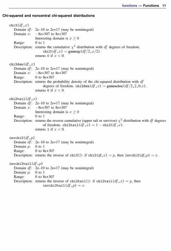
Chi-squared and noncentral chi-squared distributions
chi2(df,x)Domain df : 2e–10 to 2e+17 (may be nonintegral)Domain x: −8e+307 to 8e+307
Interesting domain is x ≥ 0Range: 0 to 1Description: returns the cumulative χ2 distribution with df degrees of freedom.
chi2(df,x) = gammap(df/2,x/2).returns 0 if x < 0.
chi2den(df,x)Domain df : 2e–10 to 2e+17 (may be nonintegral)Domain x: −8e+307 to 8e+307Range: 0 to 8e+307Description: returns the probability density of the chi-squared distribution with df
degrees of freedom. chi2den(df,x) = gammaden(df/2,2,0,x).returns 0 if x < 0.
chi2tail(df,x)Domain df : 2e–10 to 2e+17 (may be nonintegral)Domain x: −8e+307 to 8e+307
Interesting domain is x ≥ 0Range: 0 to 1Description: returns the reverse cumulative (upper tail or survivor) χ2 distribution with df degrees
of freedom. chi2tail(df,x) = 1− chi2(df,x).returns 1 if x < 0.
invchi2(df,p)Domain df : 2e–10 to 2e+17 (may be nonintegral)Domain p: 0 to 1Range: 0 to 8e+307Description: returns the inverse of chi2(): if chi2(df,x) = p, then invchi2(df,p) = x.
invchi2tail(df,p)Domain df : 2e–10 to 2e+17 (may be nonintegral)Domain p: 0 to 1Range: 0 to 8e+307Description: returns the inverse of chi2tail(): if chi2tail(df,x) = p, then
invchi2tail(df,p) = x.
12 functions — Functions
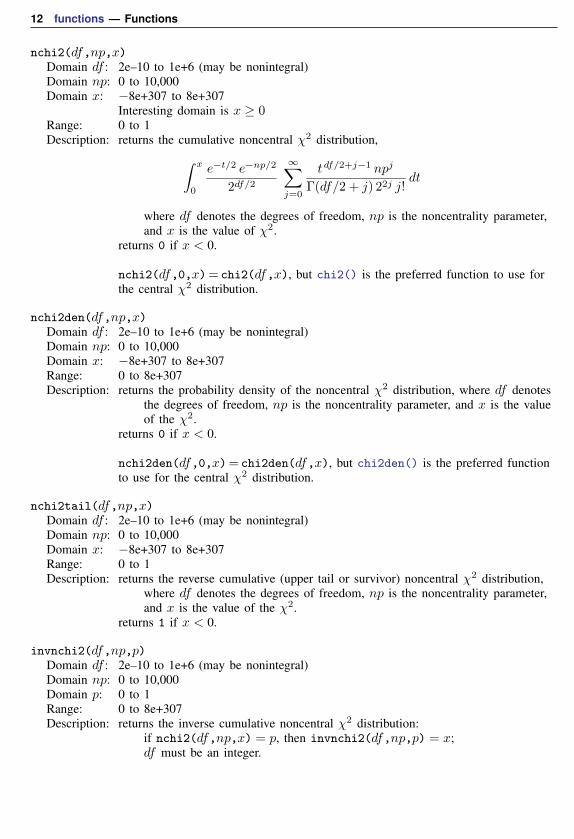
nchi2(df,np,x)Domain df : 2e–10 to 1e+6 (may be nonintegral)Domain np: 0 to 10,000Domain x: −8e+307 to 8e+307
Interesting domain is x ≥ 0Range: 0 to 1Description: returns the cumulative noncentral χ2 distribution,∫ x
0
e−t/2 e−np/2
2df/2
∞∑j=0
tdf/2+j−1 npj
Γ(df/2 + j) 22j j!dt
where df denotes the degrees of freedom, np is the noncentrality parameter,and x is the value of χ2.
returns 0 if x < 0.
nchi2(df,0,x)= chi2(df,x), but chi2() is the preferred function to use forthe central χ2 distribution.
nchi2den(df,np,x)Domain df : 2e–10 to 1e+6 (may be nonintegral)Domain np: 0 to 10,000Domain x: −8e+307 to 8e+307Range: 0 to 8e+307Description: returns the probability density of the noncentral χ2 distribution, where df denotes
the degrees of freedom, np is the noncentrality parameter, and x is the valueof the χ2.
returns 0 if x < 0.
nchi2den(df,0,x)= chi2den(df,x), but chi2den() is the preferred functionto use for the central χ2 distribution.
nchi2tail(df,np,x)Domain df : 2e–10 to 1e+6 (may be nonintegral)Domain np: 0 to 10,000Domain x: −8e+307 to 8e+307Range: 0 to 1Description: returns the reverse cumulative (upper tail or survivor) noncentral χ2 distribution,
where df denotes the degrees of freedom, np is the noncentrality parameter,and x is the value of the χ2.
returns 1 if x < 0.
invnchi2(df,np,p)Domain df : 2e–10 to 1e+6 (may be nonintegral)Domain np: 0 to 10,000Domain p: 0 to 1Range: 0 to 8e+307Description: returns the inverse cumulative noncentral χ2 distribution:
if nchi2(df,np,x) = p, then invnchi2(df,np,p) = x;df must be an integer.
functions — Functions 13
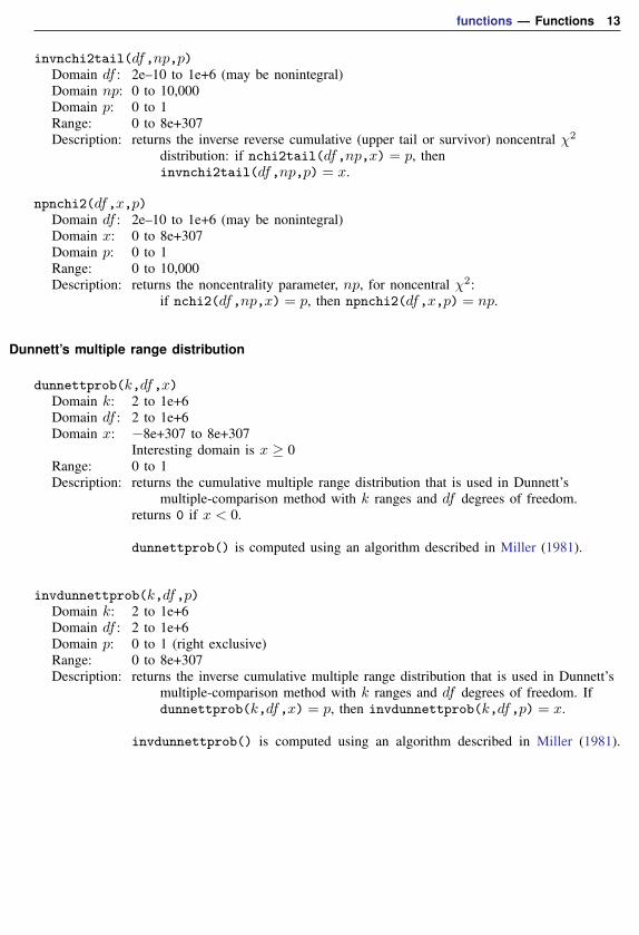
invnchi2tail(df,np,p)Domain df : 2e–10 to 1e+6 (may be nonintegral)Domain np: 0 to 10,000Domain p: 0 to 1Range: 0 to 8e+307Description: returns the inverse reverse cumulative (upper tail or survivor) noncentral χ2
distribution: if nchi2tail(df,np,x) = p, theninvnchi2tail(df,np,p) = x.
npnchi2(df,x,p)Domain df : 2e–10 to 1e+6 (may be nonintegral)Domain x: 0 to 8e+307Domain p: 0 to 1Range: 0 to 10,000Description: returns the noncentrality parameter, np, for noncentral χ2:
if nchi2(df,np,x) = p, then npnchi2(df,x,p) = np.
Dunnett’s multiple range distribution
dunnettprob(k,df,x)Domain k: 2 to 1e+6Domain df : 2 to 1e+6Domain x: −8e+307 to 8e+307
Interesting domain is x ≥ 0Range: 0 to 1Description: returns the cumulative multiple range distribution that is used in Dunnett’s
multiple-comparison method with k ranges and df degrees of freedom.returns 0 if x < 0.
dunnettprob() is computed using an algorithm described in Miller (1981).
invdunnettprob(k,df,p)Domain k: 2 to 1e+6Domain df : 2 to 1e+6Domain p: 0 to 1 (right exclusive)Range: 0 to 8e+307Description: returns the inverse cumulative multiple range distribution that is used in Dunnett’s
multiple-comparison method with k ranges and df degrees of freedom. Ifdunnettprob(k,df,x) = p, then invdunnettprob(k,df,p) = x.
invdunnettprob() is computed using an algorithm described in Miller (1981).

14 functions — Functions� �Charles William Dunnett (1921–2007) was a Canadian statistician best known for his work onmultiple-comparison procedures. He was born in Windsor, Ontario, and graduated in mathematicsand physics from McMaster University. After naval service in World War II, Dunnett’s careerincluded further graduate work, teaching, and research at Toronto, Columbia, the New York StateMaritime College, the Department of National Health and Welfare in Ottawa, Cornell, LederleLaboratories, and Aberdeen before he became Professor of Clinical Epidemiology and Biostatisticsat McMaster University in 1974. He was President and Gold Medalist of the Statistical Society ofCanada. Throughout his career, Dunnett took a keen interest in computing. According to GoogleScholar, his 1955 paper on comparing treatments with a control has been cited over 4,000 times.� �
F and noncentral F distributions
F(df1,df2,f)Domain df1: 2e–10 to 2e+17 (may be nonintegral)Domain df2: 2e–10 to 2e+17 (may be nonintegral)Domain f : −8e+307 to 8e+307
Interesting domain is f ≥ 0Range: 0 to 1Description: returns the cumulative F distribution with df1 numerator and df2 denominator
degrees of freedom: F(df1,df2,f) =∫ f0Fden(df1,df2,t) dt.
returns 0 if f < 0.
Fden(df1,df2,f)Domain df1: 1e–323 to 8e+307 (may be nonintegral)Domain df2: 1e–323 to 8e+307 (may be nonintegral)Domain f : −8e+307 to 8e+307
Interesting domain is f ≥ 0Range: 0 to 8e+307Description: returns the probability density function of the F distribution with df1 numerator
and df2 denominator degrees of freedom:
Fden(df1,df2,f) =Γ(df1+df22 )
Γ(df12 )Γ(df22 )
(df1df2
) df12
· fdf12 −1
(1 +
df1df2
f
)− 12 (df1+df2)
returns 0 if f < 0.
Ftail(df1,df2,f)Domain df1: 2e–10 to 2e+17 (may be nonintegral)Domain df2: 2e–10 to 2e+17 (may be nonintegral)Domain f : −8e+307 to 8e+307
Interesting domain is f ≥ 0Range: 0 to 1Description: returns the reverse cumulative (upper tail or survivor) F distribution with df1
numerator and df2 denominator degrees of freedom.Ftail(df1,df2,f) = 1− F(df1,df2,f).
returns 1 if f < 0.
functions — Functions 15
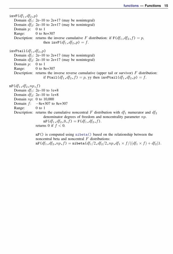
invF(df1,df2,p)Domain df1: 2e–10 to 2e+17 (may be nonintegral)Domain df2: 2e–10 to 2e+17 (may be nonintegral)Domain p: 0 to 1Range: 0 to 8e+307Description: returns the inverse cumulative F distribution: if F(df1,df2,f) = p,
then invF(df1,df2,p) = f .
invFtail(df1,df2,p)Domain df1: 2e–10 to 2e+17 (may be nonintegral)Domain df2: 2e–10 to 2e+17 (may be nonintegral)Domain p: 0 to 1Range: 0 to 8e+307Description: returns the inverse reverse cumulative (upper tail or survivor) F distribution:
if Ftail(df1,df2,f) = p, yy then invFtail(df1,df2,p) = f .
nF(df1,df2,np,f)Domain df1: 2e–10 to 1e+8Domain df2: 2e–10 to 1e+8Domain np: 0 to 10,000Domain f : −8e+307 to 8e+307Range: 0 to 1Description: returns the cumulative noncentral F distribution with df1 numerator and df2
denominator degrees of freedom and noncentrality parameter np.nF(df1,df2,0,f) = F(df1,df2,f).
returns 0 if f < 0.
nF() is computed using nibeta() based on the relationship between thenoncentral beta and noncentral F distributions:nF(df1,df2,np,f) = nibeta(df1/2,df2/2,np,df1 × f/((df1 × f) + df2)).
16 functions — Functions
nFden(df1,df2,np,f)Domain df1: 1e–323 to 8e+307 (may be nonintegral)Domain df2: 1e–323 to 8e+307 (may be nonintegral)Domain np: 0 to 1,000Domain f : −8e+307 to 8e+307
Interesting domain is f ≥ 0Range: 0 to 8e+307Description: returns the probability density function of the noncentral F distribution with df1
numerator and df2 denominator degrees of freedom and noncentralityparameter np.
returns 0 if f < 0.
nFden(df1,df2,0,f)= Fden(df1,df2,f), but Fden() is the preferred functionto use for the central F distribution.
Also, if F follows the noncentral F distribution with df1 and df2 degrees offreedom and noncentrality parameter np, then
df1F
df2 + df1F
follows a noncentral beta distribution with shape parameters a = df1/2, b = df2/2,and noncentrality parameter np, as given in nbetaden(). nFden() is computedbased on this relationship.
nFtail(df1,df2,np,f)Domain df1: 1e–323 to 8e+307 (may be nonintegral)Domain df2: 1e–323 to 8e+307 (may be nonintegral)Domain np: 0 to 1,000Domain f : −8e+307 to 8e+307
Interesting domain is f ≥ 0Range: 0 to 1Description: returns the reverse cumulative (upper tail or survivor) noncentral F distribution with
df1 numerator and df2 denominator degrees of freedom and noncentralityparameter np.
returns 1 if f < 0.
nFtail() is computed using nibeta() based on the relationship between thenoncentral beta and F distributions. See Johnson, Kotz, and Balakrishnan (1995) formore details.
invnFtail(df1,df2,np,p)Domain df1: 1e–323 to 8e+307 (may be nonintegral)Domain df2: 1e–323 to 8e+307 (may be nonintegral)Domain np: 0 to 1,000Domain p: 0 to 1Range: 0 to 8e+307Description: returns the inverse reverse cumulative (upper tail or survivor) noncentralF distribution:
if nFtail(df1,df2,np,x) = p, then invnFtail(df1,df2,np,p) = x.
functions — Functions 17
npnF(df1,df2,f,p)Domain df1: 2e–10 to 1e+6 (may be nonintegral)Domain df2: 2e–10 to 1e+6 (may be nonintegral)Domain f : 0 to 8e+307Domain p: 0 to 1Range: 0 to 1,000Description: returns the noncentrality parameter, np, for the noncentral F :
if nF(df1,df2,np,f) = p, then npnF(df1,df2,f,p) = np.
Gamma distribution
gammap(a,x)Domain a: 1e–10 to 1e+17Domain x: −8e+307 to 8e+307
Interesting domain is x ≥ 0Range: 0 to 1Description: returns the cumulative gamma distribution with shape parameter a defined by
1
Γ(a)
∫ x
0
e−tta−1 dt
returns 0 if x < 0.
The cumulative Poisson (the probability of observing k or fewer events if theexpected is x) can be evaluated as 1-gammap(k+1,x). The reverse cumulative (theprobability of observing k or more events) can be evaluated as gammap(k,x). SeePress et al. (2007, 259–266) for a more complete description and for suggested usesfor this function.
gammap() is also known as the incomplete gamma function (ratio).
Probabilities for the three-parameter gamma distribution (see gammaden()) canbe calculated by shifting and scaling x; that is, gammap(a,(x− g)/b).
gammaden(a,b,g,x)Domain a: 1e–323 to 8e+307Domain b: 1e–323 to 8e+307Domain g: −8e+307 to 8e+307Domain x: −8e+307 to 8e+307
Interesting domain is x ≥ gRange: 0 to 8e+307Description: returns the probability density function of the gamma distribution defined by
1
Γ(a)ba(x− g)a−1e−(x−g)/b
where a is the shape parameter, b is the scale parameter, and g is thelocation parameter.
returns 0 if x < g.
18 functions — Functions
gammaptail(a,x)Domain a: 1e–10 to 1e+17Domain x: −8e+307 to 8e+307
Interesting domain is x ≥ 0Range: 0 to 1Description: returns the reverse cumulative (upper tail or survivor) gamma distribution with shape
parameter a defined by
gammaptail(a,x) = 1− gammap(a,x) =
∫ ∞x
gammaden(a,t) dt
returns 1 if x < 0.
gammaptail() is also known as the complement to the incomplete gamma function(ratio).
invgammap(a,p)Domain a: 1e–10 to 1e+17Domain p: 0 to 1Range: 0 to 8e+307Description: returns the inverse cumulative gamma distribution: if gammap(a,x) = p,
then invgammap(a,p) = x.
invgammaptail(a,p)Domain a: 1e–10 to 1e+17Domain p: 0 to 1Range: 0 to 8e+307Description: returns the inverse reverse cumulative (upper tail or survivor) gamma distribution:
if gammaptail(a,x) = p, then invgammaptail(a,p) = x.
dgammapda(a,x)Domain a: 1e–7 to 1e+17Domain x: −8e+307 to 8e+307
Interesting domain is x ≥ 0Range: −16 to 0Description: returns ∂P (a,x)
∂a , where P (a, x) = gammap(a,x).returns 0 if x < 0.
dgammapdada(a,x)Domain a: 1e–7 to 1e+17Domain x: −8e+307 to 8e+307
Interesting domain is x ≥ 0Range: −0.02 to 4.77e+5Description: returns ∂2P (a,x)
∂a2 , where P (a, x) = gammap(a,x).returns 0 if x < 0.
functions — Functions 19
dgammapdadx(a,x)Domain a: 1e–7 to 1e+17Domain x: −8e+307 to 8e+307
Interesting domain is x ≥ 0Range: −0.04 to 8e+307Description: returns ∂2P (a,x)
∂a∂x , where P (a, x) = gammap(a,x).returns 0 if x < 0.
dgammapdx(a,x)Domain a: 1e–10 to 1e+17Domain x: −8e+307 to 8e+307
Interesting domain is x ≥ 0Range: 0 to 8e+307Description: returns ∂P (a,x)
∂x , where P (a, x) = gammap(a,x).returns 0 if x < 0.
dgammapdxdx(a,x)Domain a: 1e–10 to 1e+17Domain x: −8e+307 to 8e+307
Interesting domain is x ≥ 0Range: 0 to 1e+40Description: returns ∂2P (a,x)
∂x2 , where P (a, x) = gammap(a,x).returns 0 if x < 0.
Hypergeometric distribution
hypergeometric(N,K,n,k)Domain N : 2 to 1e+5Domain K: 1 to N−1Domain n: 1 to N−1Domain k: max(0,n−N +K) to min(K,n)Range: 0 to 1Description: returns the cumulative probability of the hypergeometric distribution. N is the
population size, K is the number of elements in the population that have theattribute of interest, and n is the sample size. Returned is the probabilityof observing k or fewer elements from a sample of size n that havethe attribute of interest.
hypergeometricp(N,K,n,k)Domain N : 2 to 1e+5Domain K: 1 to N−1Domain n: 1 to N−1Domain k: max(0,n−N +K) to min(K,n)Range: 0 to 1 (right exclusive)Description: returns the hypergeometric probability of k successes (where success is obtaining
an element with the attribute of interest) out of a sample of size n, froma population of size N containing K elements that have the attribute of interest.
20 functions — Functions
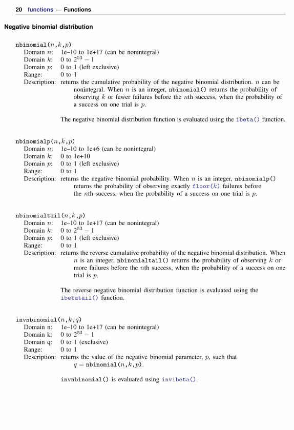
Negative binomial distribution
nbinomial(n,k,p)Domain n: 1e–10 to 1e+17 (can be nonintegral)Domain k: 0 to 253 − 1Domain p: 0 to 1 (left exclusive)Range: 0 to 1Description: returns the cumulative probability of the negative binomial distribution. n can be
nonintegral. When n is an integer, nbinomial() returns the probability ofobserving k or fewer failures before the nth success, when the probability ofa success on one trial is p.
The negative binomial distribution function is evaluated using the ibeta() function.
nbinomialp(n,k,p)Domain n: 1e–10 to 1e+6 (can be nonintegral)Domain k: 0 to 1e+10Domain p: 0 to 1 (left exclusive)Range: 0 to 1Description: returns the negative binomial probability. When n is an integer, nbinomialp()
returns the probability of observing exactly floor(k) failures beforethe nth success, when the probability of a success on one trial is p.
nbinomialtail(n,k,p)Domain n: 1e–10 to 1e+17 (can be nonintegral)Domain k: 0 to 253 − 1Domain p: 0 to 1 (left exclusive)Range: 0 to 1Description: returns the reverse cumulative probability of the negative binomial distribution. When
n is an integer, nbinomialtail() returns the probability of observing k ormore failures before the nth success, when the probability of a success on onetrial is p.
The reverse negative binomial distribution function is evaluated using theibetatail() function.
invnbinomial(n,k,q)Domain n: 1e–10 to 1e+17 (can be nonintegral)Domain k: 0 to 253 − 1Domain q: 0 to 1 (exclusive)Range: 0 to 1Description: returns the value of the negative binomial parameter, p, such that
q = nbinomial(n,k,p).
invnbinomial() is evaluated using invibeta().
functions — Functions 21
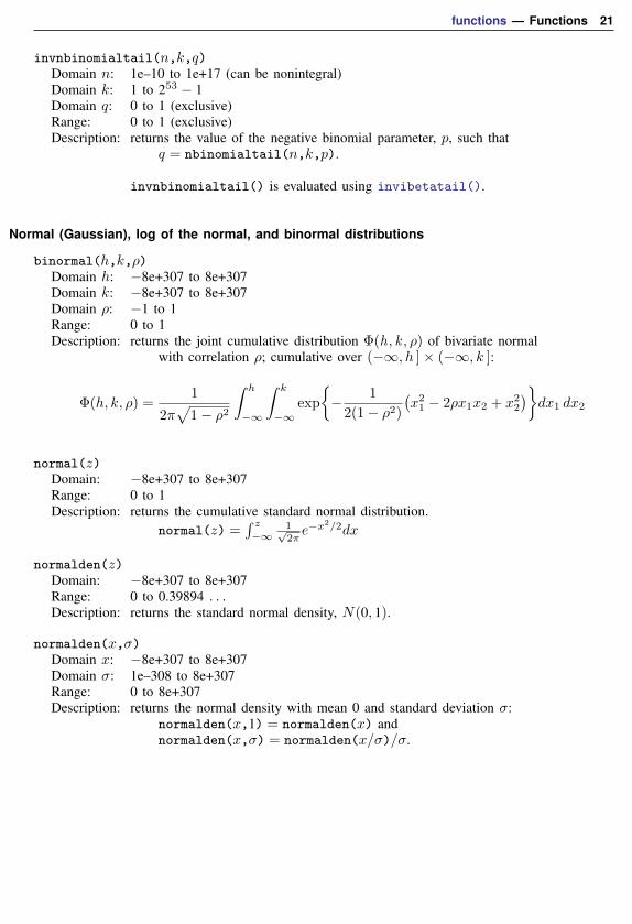
invnbinomialtail(n,k,q)Domain n: 1e–10 to 1e+17 (can be nonintegral)Domain k: 1 to 253 − 1Domain q: 0 to 1 (exclusive)Range: 0 to 1 (exclusive)Description: returns the value of the negative binomial parameter, p, such that
q = nbinomialtail(n,k,p).
invnbinomialtail() is evaluated using invibetatail().
Normal (Gaussian), log of the normal, and binormal distributions
binormal(h,k,ρ)Domain h: −8e+307 to 8e+307Domain k: −8e+307 to 8e+307Domain ρ: −1 to 1Range: 0 to 1Description: returns the joint cumulative distribution Φ(h, k , ρ) of bivariate normal
with correlation ρ; cumulative over (−∞, h ]× (−∞, k ]:
Φ(h, k, ρ) =1
2π√
1− ρ2
∫ h
−∞
∫ k
−∞exp
{− 1
2(1− ρ2)
(x21 − 2ρx1x2 + x22
)}dx1 dx2
normal(z)Domain: −8e+307 to 8e+307Range: 0 to 1Description: returns the cumulative standard normal distribution.
normal(z) =∫ z−∞
1√2πe−x
2/2dx
normalden(z)Domain: −8e+307 to 8e+307Range: 0 to 0.39894 . . .Description: returns the standard normal density, N(0, 1).
normalden(x,σ)Domain x: −8e+307 to 8e+307Domain σ: 1e–308 to 8e+307Range: 0 to 8e+307Description: returns the normal density with mean 0 and standard deviation σ:
normalden(x,1) = normalden(x) andnormalden(x,σ) = normalden(x/σ)/σ.
22 functions — Functions
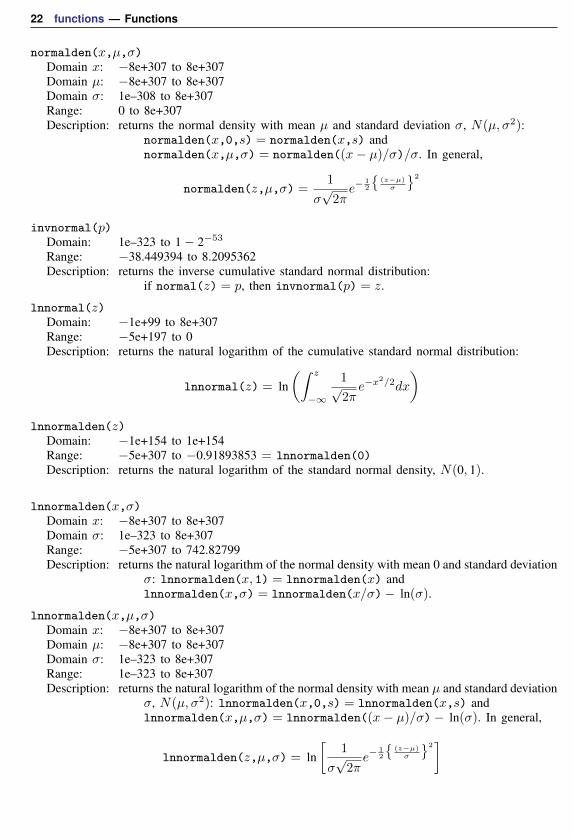
normalden(x,µ,σ)Domain x: −8e+307 to 8e+307Domain µ: −8e+307 to 8e+307Domain σ: 1e–308 to 8e+307Range: 0 to 8e+307Description: returns the normal density with mean µ and standard deviation σ, N(µ, σ2):
normalden(x,0,s) = normalden(x,s) andnormalden(x,µ,σ) = normalden((x− µ)/σ)/σ. In general,
normalden(z,µ,σ) =1
σ√
2πe−
12
{(z−µ)σ
}2
invnormal(p)Domain: 1e–323 to 1− 2−53
Range: −38.449394 to 8.2095362Description: returns the inverse cumulative standard normal distribution:
if normal(z) = p, then invnormal(p) = z.
lnnormal(z)Domain: −1e+99 to 8e+307Range: −5e+197 to 0Description: returns the natural logarithm of the cumulative standard normal distribution:
lnnormal(z) = ln(∫ z
−∞
1√2πe−x
2/2dx
)lnnormalden(z)
Domain: −1e+154 to 1e+154Range: −5e+307 to −0.91893853 = lnnormalden(0)Description: returns the natural logarithm of the standard normal density, N(0, 1).
lnnormalden(x,σ)Domain x: −8e+307 to 8e+307Domain σ: 1e–323 to 8e+307Range: −5e+307 to 742.82799Description: returns the natural logarithm of the normal density with mean 0 and standard deviation
σ: lnnormalden(x, 1) = lnnormalden(x) andlnnormalden(x,σ) = lnnormalden(x/σ)− ln(σ).
lnnormalden(x,µ,σ)Domain x: −8e+307 to 8e+307Domain µ: −8e+307 to 8e+307Domain σ: 1e–323 to 8e+307Range: 1e–323 to 8e+307Description: returns the natural logarithm of the normal density with mean µ and standard deviation
σ, N(µ, σ2): lnnormalden(x,0,s) = lnnormalden(x,s) andlnnormalden(x,µ,σ) = lnnormalden((x− µ)/σ)− ln(σ). In general,
lnnormalden(z,µ,σ) = ln[
1
σ√
2πe−
12
{(z−µ)σ
}2]
functions — Functions 23
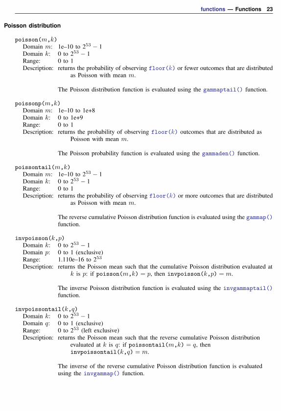
Poisson distribution
poisson(m,k)Domain m: 1e–10 to 253 − 1Domain k: 0 to 253 − 1Range: 0 to 1Description: returns the probability of observing floor(k) or fewer outcomes that are distributed
as Poisson with mean m.
The Poisson distribution function is evaluated using the gammaptail() function.
poissonp(m,k)Domain m: 1e–10 to 1e+8Domain k: 0 to 1e+9Range: 0 to 1Description: returns the probability of observing floor(k) outcomes that are distributed as
Poisson with mean m.
The Poisson probability function is evaluated using the gammaden() function.
poissontail(m,k)Domain m: 1e–10 to 253 − 1Domain k: 0 to 253 − 1Range: 0 to 1Description: returns the probability of observing floor(k) or more outcomes that are distributed
as Poisson with mean m.
The reverse cumulative Poisson distribution function is evaluated using the gammap()function.
invpoisson(k,p)Domain k: 0 to 253 − 1Domain p: 0 to 1 (exclusive)Range: 1.110e–16 to 253
Description: returns the Poisson mean such that the cumulative Poisson distribution evaluated atk is p: if poisson(m,k) = p, then invpoisson(k,p) = m.
The inverse Poisson distribution function is evaluated using the invgammaptail()function.
invpoissontail(k,q)Domain k: 0 to 253 − 1Domain q: 0 to 1 (exclusive)Range: 0 to 253 (left exclusive)Description: returns the Poisson mean such that the reverse cumulative Poisson distribution
evaluated at k is q: if poissontail(m,k) = q, theninvpoissontail(k,q) = m.
The inverse of the reverse cumulative Poisson distribution function is evaluatedusing the invgammap() function.
24 functions — Functions
Student’s t and noncentral Student’s t distributions
t(df,t)Domain df : 2e+10 to 2e+17 (may be nonintegral)Domain t: −8e+307 to 8e+307Range: 0 to 1Description: returns the cumulative Student’s t distribution with df degrees of freedom.
tden(df,t)Domain df : 1e–323 to 8e+307(may be nonintegral)Domain t: −8e+307 to 8e+307Range: 0 to 0.39894 . . .Description: returns the probability density function of Student’s t distribution:
tden(df,t) =Γ{(df + 1)/2}√πdfΓ(df/2)
·(1 + t2/df)−(df+1)/2
ttail(df,t)Domain df : 2e–10 to 2e+17 (may be nonintegral)Domain t: −8e+307 to 8e+307Range: 0 to 1Description: returns the reverse cumulative (upper tail or survivor) Student’s t distribution;
it returns the probability T > t:
ttail(df,t) =
∫ ∞t
Γ{(df + 1)/2}√πdfΓ(df/2)
·(1 + x2/df)−(df+1)/2 dx
invt(df,p)Domain df : 2e–10 to 2e+17 (may be nonintegral)Domain p: 0 to 1Range: −8e+307 to 8e+307Description: returns the inverse cumulative Student’s t distribution:
if t(df,t) = p, then invt(df,p) = t.
invttail(df,p)Domain df : 2e–10 to 2e+17 (may be nonintegral)Domain p: 0 to 1Range: −8e+307 to 8e+307Description: returns the inverse reverse cumulative (upper tail or survivor) Student’s t distribution:
if ttail(df,t) = p, then invttail(df,p) = t.
nt(df,np,t)Domain df : 1e–100 to 1e+10 (may be nonintegral)Domain np: −1,000 to 1,000Domain t: −8e+307 to 8e+307Range: 0 to 1Description: returns the cumulative noncentral Student’s t distribution with df degrees of freedom
and noncentrality parameter np. nt(df,0,t) = t(df,t).
functions — Functions 25
ntden(df,np,t)Domain df : 1e–100 to 1e+10 (may be nonintegral)Domain np: −1,000 to 1,000Domain t: −8e+307 to 8e+307Range: 0 to 0.39894 . . .Description: returns the probability density function of the noncentral Student’s t distribution with
df degrees of freedom and noncentrality parameter np.
nttail(df,np,t)Domain df : 1e–100 to 1e+10 (may be nonintegral)Domain np: −1,000 to 1,000Domain t: −8e+307 to 8e+307Range: 0 to 1Description: returns the reverse cumulative (upper tail or survivor) noncentral
Student’s t distribution with df degrees of freedom andnoncentrality parameter np.
invnttail(df,np,p)Domain df : 1 to 1e+6 (may be nonintegral)Domain np: −1,000 to 1,000Domain p: 0 to 1Range: −8e+10 to 8e+10Description: returns the inverse reverse cumulative (upper tail or survivor) noncentral
Student’s t distribution: if nttail(df,np,t) = p,then invnttail(df,np,p) = t.
npnt(df,t,p)Domain df : 1e–100 to 1e+8 (may be nonintegral)Domain t: −8e+307 to 8e+307Domain p: 0 to 1Range: −1,000 to 1,000Description: returns the noncentrality parameter, np, for the noncentral Student’s t distribution:
if nt(df,np,t) = p, then npnt(df,t,p) = np.
Tukey’s Studentized range distribution
tukeyprob(k,df,x)Domain k: 2 to 1e+6Domain df : 2 to 1e+6Domain x: −8e+307 to 8e+307
Interesting domain is x ≥ 0Range: 0 to 1Description: returns the cumulative Tukey’s Studentized range distribution with k ranges and
df degrees of freedom. If df is a missing value, then the normal distributionis used instead of Student’s t.
returns 0 if x < 0.
tukeyprob() is computed using an algorithm described in Miller (1981).
26 functions — Functions
invtukeyprob(k,df,p)Domain k: 2 to 1e+6Domain df : 2 to 1e+6Domain p: 0 to 1Range: 0 to 8e+307Description: returns the inverse cumulative Tukey’s Studentized range distribution with k ranges
and df degrees of freedom. If df is a missing value, then the normal distributionis used instead of Student’s t. If tukeyprob(k,df,x) = p, theninvtukeyprob(k,df,p) = x.
invtukeyprob() is computed using an algorithm described in Miller (1981).
Random-number functions
runiform()Range: 0 to nearly 1 (0 to 1− 2−32)Description: returns uniform random variates.
runiform() returns uniformly distributed random variates on the interval[ 0, 1). runiform() takes no arguments, but the parentheses must be typed.runiform() can be seeded with the set seed command; see the technical note atthe end of this subsection. (See Matrix functions for the related matuniform()matrix function.)
To generate random variates over the interval [ a, b), usea+(b-a)*runiform().
To generate random integers over [ a, b ], use a+int((b-a+1)*runiform()).
rbeta(a,b)Domain a: 0.05 to 1e+5Domain b: 0.15 to 1e+5Range: 0 to 1 (exclusive)Description: returns beta(a,b) random variates, where a and b are the beta distribution shape
parameters.
Besides the standard methodology for generating random variates from a givendistribution, rbeta() uses the specialized algorithms of Johnk (Gentle 2003),Atkinson and Whittaker (1970, 1976), Devroye (1986), andSchmeiser and Babu (1980).
functions — Functions 27
rbinomial(n,p)Domain n: 1 to 1e+11Domain p: 1e–8 to 1−1e–8Range: 0 to nDescription: returns binomial(n,p) random variates, where n is the number of trials and p is the
success probability.
Besides the standard methodology for generating random variates from a givendistribution, rbinomial() uses the specialized algorithms ofKachitvichyanukul (1982), Kachitvichyanukul and Schmeiser (1988), andKemp (1986).
rchi2(df)Domain df : 2e–4 to 2e+8Range: 0 to c(maxdouble)Description: returns chi-squared, with df degrees of freedom, random variates.
rgamma(a,b)Domain a: 1e–4 to 1e+8Domain b: c(smallestdouble) to c(maxdouble)Range: 0 to c(maxdouble)Description: returns gamma(a,b) random variates, where a is the gamma shape parameter and b
is the scale parameter.
Methods for generating gamma variates are taken from Ahrens and Dieter (1974),Best (1983), and Schmeiser and Lal (1980).
rhypergeometric(N,K,n)Domain N : 2 to 1e+6Domain K: 1 to N−1Domain n: 1 to N−1Range: max(0,n−N +K) to min(K,n)Description: returns hypergeometric random variates. The distribution parameters are integer
valued, where N is the population size, K is the number of elements inthe population that have the attribute of interest, and n is the sample size.
Besides the standard methodology for generating random variates from a givendistribution, rhypergeometric() uses the specialized algorithms ofKachitvichyanukul (1982) and Kachitvichyanukul and Schmeiser (1985).
rnbinomial(n,p)Domain n: 1e–4 to 1e+5Domain p: 1e–4 to 1−1e–4Range: 0 to 253 − 1Description: returns negative binomial random variates. If n is integer valued, rnbinomial()
returns the number of failures before the nth success, where the probability ofsuccess on a single trial is p. n can also be nonintegral.
rnormal()Range: c(mindouble) to c(maxdouble)Description: returns standard normal (Gaussian) random variates, that is, variates from a normal
distribution with a mean of 0 and a standard deviation of 1.
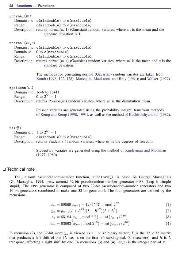
28 functions — Functions
rnormal(m)Domain m: c(mindouble) to c(maxdouble)Range: c(mindouble) to c(maxdouble)Description: returns normal(m,1) (Gaussian) random variates, where m is the mean and the
standard deviation is 1.
rnormal(m,s)Domain m: c(mindouble) to c(maxdouble)Domain s: 0 to c(maxdouble)Range: c(mindouble) to c(maxdouble)Description: returns normal(m,s) (Gaussian) random variates, where m is the mean and s is the
standard deviation.
The methods for generating normal (Gaussian) random variates are taken fromKnuth (1998, 122–128); Marsaglia, MacLaren, and Bray (1964); and Walker (1977).
rpoisson(m)Domain m: 1e–6 to 1e+11Range: 0 to 253 − 1Description: returns Poisson(m) random variates, where m is the distribution mean.
Poisson variates are generated using the probability integral transform methodsof Kemp and Kemp (1990, 1991), as well as the method of Kachitvichyanukul (1982).
rt(df)Domain df : 1 to 253 − 1Range: c(mindouble) to c(maxdouble)Description: returns Student’s t random variates, where df is the degrees of freedom.
Student’s t variates are generated using the method of Kinderman and Monahan(1977, 1980).
Technical note
The uniform pseudorandom-number function, runiform(), is based on George Marsaglia’s(G. Marsaglia, 1994, pers. comm.) 32-bit pseudorandom-number generator KISS (keep it simplestupid). The KISS generator is composed of two 32-bit pseudorandom-number generators and two16-bit generators (combined to make one 32-bit generator). The four generators are defined by therecursions
xn = 69069xn−1 + 1234567 mod 232 (1)
yn = yn−1(I + L13)(I +R17)(I + L5) (2)
zn = 65184(zn−1 mod 216
)+ int
(zn−1/2
16)
(3)
wn = 63663(wn−1 mod 216
)+ int
(wn−1/2
16)
(4)
In recursion (2), the 32-bit word yn is viewed as a 1 × 32 binary vector; L is the 32 × 32 matrixthat produces a left shift of one (L has 1s on the first left subdiagonal, 0s elsewhere); and R is Ltranspose, affecting a right shift by one. In recursions (3) and (4), int(x) is the integer part of x.
functions — Functions 29
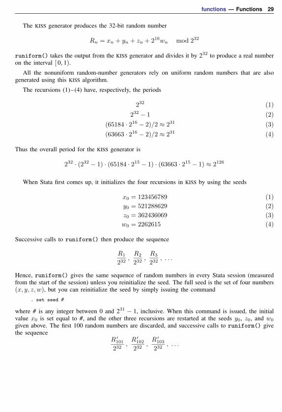
The KISS generator produces the 32-bit random number
Rn = xn + yn + zn + 216wn mod 232
runiform() takes the output from the KISS generator and divides it by 232 to produce a real numberon the interval [ 0, 1).
All the nonuniform random-number generators rely on uniform random numbers that are alsogenerated using this KISS algorithm.
The recursions (1)–(4) have, respectively, the periods
232 (1)
232 − 1 (2)
(65184 · 216 − 2)/2 ≈ 231 (3)
(63663 · 216 − 2)/2 ≈ 231 (4)
Thus the overall period for the KISS generator is
232 · (232 − 1) · (65184 · 215 − 1) · (63663 · 215 − 1) ≈ 2126
When Stata first comes up, it initializes the four recursions in KISS by using the seeds
x0 = 123456789 (1)
y0 = 521288629 (2)
z0 = 362436069 (3)
w0 = 2262615 (4)
Successive calls to runiform() then produce the sequence
R1
232,R2
232,R3
232, . . .
Hence, runiform() gives the same sequence of random numbers in every Stata session (measuredfrom the start of the session) unless you reinitialize the seed. The full seed is the set of four numbers(x, y, z, w), but you can reinitialize the seed by simply issuing the command
. set seed #
where # is any integer between 0 and 231 − 1, inclusive. When this command is issued, the initialvalue x0 is set equal to #, and the other three recursions are restarted at the seeds y0, z0, and w0
given above. The first 100 random numbers are discarded, and successive calls to runiform() givethe sequence
R ′101232
,R ′102232
,R ′103232
, . . .
30 functions — Functions
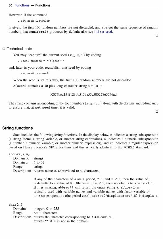
However, if the command
. set seed 123456789
is given, the first 100 random numbers are not discarded, and you get the same sequence of randomnumbers that runiform() produces by default; also see [R] set seed.
Technical noteYou may “capture” the current seed (x, y, z, w) by coding
. local curseed = "‘c(seed)’"
and, later in your code, reestablish that seed by coding
. set seed ‘curseed’
When the seed is set this way, the first 100 random numbers are not discarded.
c(seed) contains a 30-plus long character string similar to
X075bcd151f123bb5159a55e50022865746ad
The string contains an encoding of the four numbers (x, y, z, w) along with checksums and redundancyto ensure that, at set seed time, it is valid.
String functions
Stata includes the following string functions. In the display below, s indicates a string subexpression(a string literal, a string variable, or another string expression), n indicates a numeric subexpression(a number, a numeric variable, or another numeric expression), and re indicates a regular expressionbased on Henry Spencer’s NFA algorithms and this is nearly identical to the POSIX.2 standard.
abbrev(s,n)Domain s: stringsDomain n: 5 to 32Range: stringsDescription: returns name s, abbreviated to n characters.
If any of the characters of s are a period, “.”, and n < 8, then the value ofn defaults to a value of 8. Otherwise, if n < 5, then n defaults to a value of 5.If n is missing, abbrev() will return the entire string s. abbrev() istypically used with variable names and variable names with factor-variable ortime-series operators (the period case). abbrev("displacement",8) is displa~t.
char(n)Domain: integers 0 to 255Range: ASCII charactersDescription: returns the character corresponding to ASCII code n.
returns "" if n is not in the domain.
functions — Functions 31
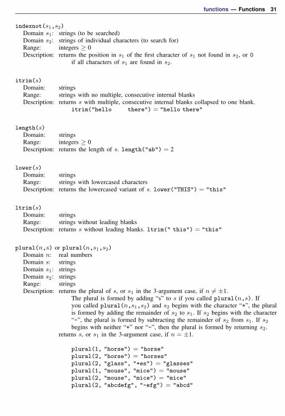
indexnot(s1,s2)Domain s1: strings (to be searched)Domain s2: strings of individual characters (to search for)Range: integers ≥ 0Description: returns the position in s1 of the first character of s1 not found in s2, or 0
if all characters of s1 are found in s2.
itrim(s)Domain: stringsRange: strings with no multiple, consecutive internal blanksDescription: returns s with multiple, consecutive internal blanks collapsed to one blank.
itrim("hello there") = "hello there"
length(s)Domain: stringsRange: integers ≥ 0Description: returns the length of s. length("ab") = 2
lower(s)Domain: stringsRange: strings with lowercased charactersDescription: returns the lowercased variant of s. lower("THIS") = "this"
ltrim(s)Domain: stringsRange: strings without leading blanksDescription: returns s without leading blanks. ltrim(" this") = "this"
plural(n,s) or plural(n,s1,s2)Domain n: real numbersDomain s: stringsDomain s1: stringsDomain s2: stringsRange: stringsDescription: returns the plural of s, or s1 in the 3-argument case, if n 6= ±1.
The plural is formed by adding “s” to s if you called plural(n,s). Ifyou called plural(n,s1,s2) and s2 begins with the character “+”, the pluralis formed by adding the remainder of s2 to s1. If s2 begins with the character“-”, the plural is formed by subtracting the remainder of s2 from s1. If s2begins with neither “+” nor “-”, then the plural is formed by returning s2.
returns s, or s1 in the 3-argument case, if n = ±1.
plural(1, "horse") = "horse"plural(2, "horse") = "horses"plural(2, "glass", "+es") = "glasses"plural(1, "mouse", "mice") = "mouse"plural(2, "mouse", "mice") = "mice"plural(2, "abcdefg", "-efg") = "abcd"
32 functions — Functions
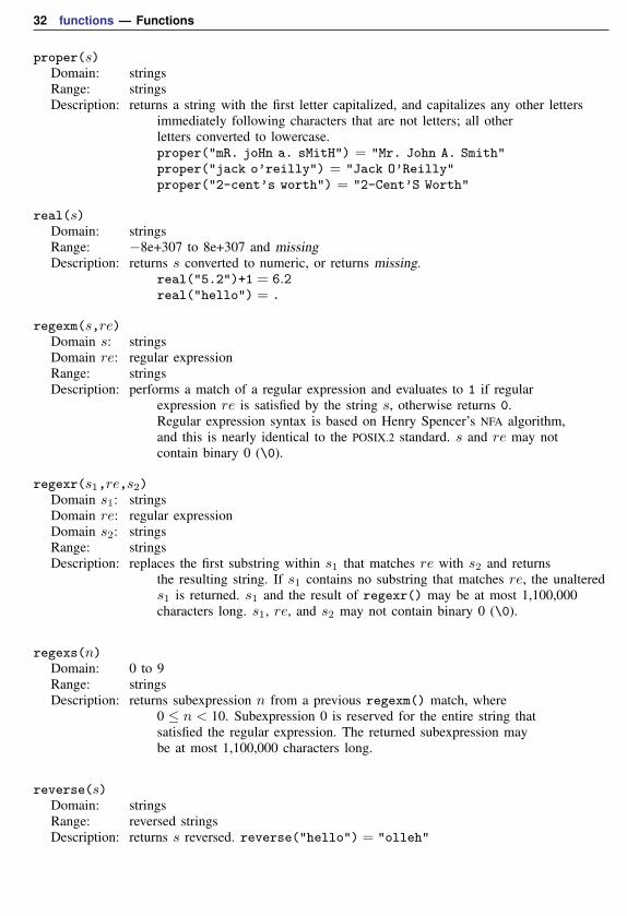
proper(s)Domain: stringsRange: stringsDescription: returns a string with the first letter capitalized, and capitalizes any other letters
immediately following characters that are not letters; all otherletters converted to lowercase.proper("mR. joHn a. sMitH") = "Mr. John A. Smith"proper("jack o’reilly") = "Jack O’Reilly"proper("2-cent’s worth") = "2-Cent’S Worth"
real(s)Domain: stringsRange: −8e+307 to 8e+307 and missingDescription: returns s converted to numeric, or returns missing.
real("5.2")+1 = 6.2real("hello") = .
regexm(s,re)Domain s: stringsDomain re: regular expressionRange: stringsDescription: performs a match of a regular expression and evaluates to 1 if regular
expression re is satisfied by the string s, otherwise returns 0.Regular expression syntax is based on Henry Spencer’s NFA algorithm,and this is nearly identical to the POSIX.2 standard. s and re may notcontain binary 0 (\0).
regexr(s1,re,s2)Domain s1: stringsDomain re: regular expressionDomain s2: stringsRange: stringsDescription: replaces the first substring within s1 that matches re with s2 and returns
the resulting string. If s1 contains no substring that matches re, the unaltereds1 is returned. s1 and the result of regexr() may be at most 1,100,000characters long. s1, re, and s2 may not contain binary 0 (\0).
regexs(n)Domain: 0 to 9Range: stringsDescription: returns subexpression n from a previous regexm() match, where
0 ≤ n < 10. Subexpression 0 is reserved for the entire string thatsatisfied the regular expression. The returned subexpression maybe at most 1,100,000 characters long.
reverse(s)Domain: stringsRange: reversed stringsDescription: returns s reversed. reverse("hello") = "olleh"
functions — Functions 33
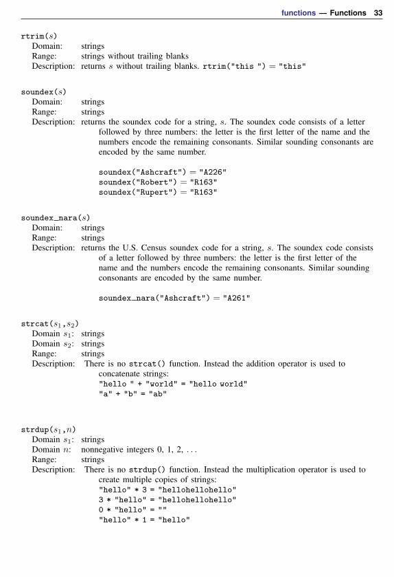
rtrim(s)Domain: stringsRange: strings without trailing blanksDescription: returns s without trailing blanks. rtrim("this ") = "this"
soundex(s)Domain: stringsRange: stringsDescription: returns the soundex code for a string, s. The soundex code consists of a letter
followed by three numbers: the letter is the first letter of the name and thenumbers encode the remaining consonants. Similar sounding consonants areencoded by the same number.
soundex("Ashcraft") = "A226"soundex("Robert") = "R163"soundex("Rupert") = "R163"
soundex nara(s)Domain: stringsRange: stringsDescription: returns the U.S. Census soundex code for a string, s. The soundex code consists
of a letter followed by three numbers: the letter is the first letter of thename and the numbers encode the remaining consonants. Similar soundingconsonants are encoded by the same number.
soundex nara("Ashcraft") = "A261"
strcat(s1,s2)Domain s1: stringsDomain s2: stringsRange: stringsDescription: There is no strcat() function. Instead the addition operator is used to
concatenate strings:"hello " + "world" = "hello world""a" + "b" = "ab"
strdup(s1,n)Domain s1: stringsDomain n: nonnegative integers 0, 1, 2, . . .Range: stringsDescription: There is no strdup() function. Instead the multiplication operator is used to
create multiple copies of strings:"hello" * 3 = "hellohellohello"3 * "hello" = "hellohellohello"0 * "hello" = """hello" * 1 = "hello"
34 functions — Functions
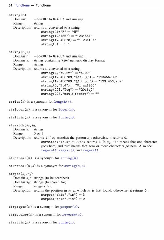
string(n)Domain: −8e+307 to 8e+307 and missingRange: stringsDescription: returns n converted to a string.
string(4)+"F" = "4F"string(1234567) = "1234567"string(12345678) = "1.23e+07"string(.) = "."
string(n,s)Domain n: −8e+307 to 8e+307 and missingDomain s: strings containing % fmt numeric display formatRange: stringsDescription: returns n converted to a string.
string(4,"%9.2f") = "4.00"string(123456789,"%11.0g") = "123456789"string(123456789,"%13.0gc") = "123,456,789"string(0,"%td") = "01jan1960"string(225,"%tq") = "2016q2"string(225,"not a format") = ""
strlen(s) is a synonym for length(s).
strlower(x) is a synonym for lower(x).
strltrim(x) is a synonym for ltrim(x).
strmatch(s1,s2)Domain s: stringsRange: 0 or 1Description: returns 1 if s1 matches the pattern s2; otherwise, it returns 0.
strmatch("17.4","1??4") returns 1. In s2, "?" means that one charactergoes here, and "*" means that zero or more characters go here. Also seeregexm(), regexr(), and regexs().
strofreal(n) is a synonym for string(n).
strofreal(n,s) is a synonym for string(n,s).
strpos(s1,s2)Domain s1: strings (to be searched)Domain s2: strings (to search for)Range: integers ≥ 0Description: returns the position in s1 at which s2 is first found; otherwise, it returns 0.
strpos("this","is") = 3strpos("this","it") = 0
strproper(x) is a synonym for proper(x).
strreverse(x) is a synonym for reverse(x).
strrtrim(x) is a synonym for rtrim(x).
functions — Functions 35
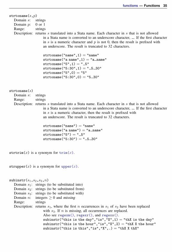
strtoname(s,p)Domain s: stringsDomain p: 0 or 1Range: stringsDescription: returns s translated into a Stata name. Each character in s that is not allowed
in a Stata name is converted to an underscore character, . If the first characterin s is a numeric character and p is not 0, then the result is prefixed withan underscore. The result is truncated to 32 characters.
strtoname("name",1) = "name"strtoname("a name",1) = "a name"strtoname("5",1) = " 5"strtoname("5:30",1) = " 5 30"strtoname("5",0) = "5"strtoname("5:30",0) = "5 30"
strtoname(s)Domain s: stringsRange: stringsDescription: returns s translated into a Stata name. Each character in s that is not allowed
in a Stata name is converted to an underscore character, . If the first characterin s is a numeric character, then the result is prefixed withan underscore. The result is truncated to 32 characters.
strtoname("name") = "name"strtoname("a name") = "a name"strtoname("5") = " 5"strtoname("5:30") = " 5 30"
strtrim(x) is a synonym for trim(x).
strupper(x) is a synonym for upper(x).
subinstr(s1,s2,s3,n)Domain s1: strings (to be substituted into)Domain s2: strings (to be substituted from)Domain s3: strings (to be substituted with)Domain n: integers ≥ 0 and missingRange: stringsDescription: returns s1, where the first n occurrences in s1 of s2 have been replaced
with s3. If n is missing, all occurrences are replaced.Also see regexm(), regexr(), and regexs().subinstr("this is the day","is","X",1) = "thX is the day"subinstr("this is the hour","is","X",2) = "thX X the hour"subinstr("this is this","is","X",.) = "thX X thX"
36 functions — Functions
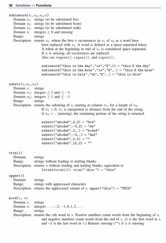
subinword(s1,s2,s3,n)Domain s1: strings (to be substituted for)Domain s2: strings (to be substituted from)Domain s3: strings (to be substituted with)Domain n: integers ≥ 0 and missingRange: stringsDescription: returns s1, where the first n occurrences in s1 of s2 as a word have
been replaced with s3. A word is defined as a space-separated token.A token at the beginning or end of s1 is considered space-separated.If n is missing, all occurrences are replaced.Also see regexm(), regexr(), and regexs().
subinword("this is the day","is","X",1) = "this X the day"subinword("this is the hour","is","X",.) = "this X the hour"subinword("this is this","th","X",.) = "this is this"
substr(s,n1,n2)Domain s: stringsDomain n1: integers ≥ 1 and ≤ −1Domain n2: integers ≥ 1 and ≤ −1Range: stringsDescription: returns the substring of s, starting at column n1, for a length of n2.
If n1 < 0, n1 is interpreted as distance from the end of the string;if n2 = . (missing), the remaining portion of the string is returned.
substr("abcdef",2,3) = "bcd"substr("abcdef",-3,2) = "de"substr("abcdef",2,.) = "bcdef"substr("abcdef",-3,.) = "def"substr("abcdef",2,0) = ""substr("abcdef",15,2) = ""
trim(s)Domain: stringsRange: strings without leading or trailing blanksDescription: returns s without leading and trailing blanks; equivalent to
ltrim(rtrim(s)). trim(" this ") = "this"
upper(s)Domain: stringsRange: strings with uppercased charactersDescription: returns the uppercased variant of s. upper("this") = "THIS"
word(s, n)Domain s: stringsDomain n: integers . . . ,−2,−1, 0, 1, 2, . . .Range: stringsDescription: returns the nth word in s. Positive numbers count words from the beginning of s,
and negative numbers count words from the end of s. (1 is the first word in s,and -1 is the last word in s.) Returns missing ("") if n is missing.
functions — Functions 37
wordcount(s)Domain: stringsRange: nonnegative integers 0, 1, 2, . . .Description: returns the number of words in s. A word is a set of characters that start
and terminate with spaces, start with the beginning of the string,or terminate with the end of the string.
Programming functions
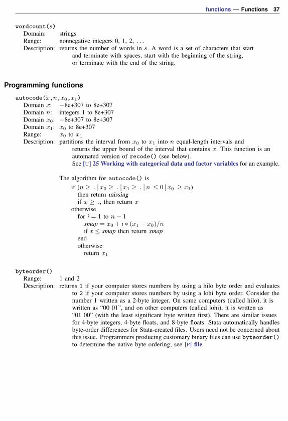
autocode(x,n,x0,x1)Domain x: −8e+307 to 8e+307Domain n: integers 1 to 8e+307Domain x0: −8e+307 to 8e+307Domain x1: x0 to 8e+307Range: x0 to x1Description: partitions the interval from x0 to x1 into n equal-length intervals and
returns the upper bound of the interval that contains x. This function is anautomated version of recode() (see below).See [U] 25 Working with categorical data and factor variables for an example.
The algorithm for autocode() isif (n ≥ . |x0 ≥ . |x1 ≥ . |n ≤ 0 |x0 ≥ x1)
then return missingif x ≥ ., then return x
otherwisefor i = 1 to n− 1
xmap = x0 + i ∗ (x1 − x0)/nif x ≤ xmap then return xmap
endotherwise
return x1
byteorder()Range: 1 and 2Description: returns 1 if your computer stores numbers by using a hilo byte order and evaluates
to 2 if your computer stores numbers by using a lohi byte order. Consider thenumber 1 written as a 2-byte integer. On some computers (called hilo), it iswritten as “00 01”, and on other computers (called lohi), it is written as“01 00” (with the least significant byte written first). There are similar issuesfor 4-byte integers, 4-byte floats, and 8-byte floats. Stata automatically handlesbyte-order differences for Stata-created files. Users need not be concerned aboutthis issue. Programmers producing customary binary files can use byteorder()to determine the native byte ordering; see [P] file.
38 functions — Functions
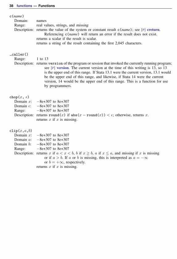
c(name)Domain: namesRange: real values, strings, and missingDescription: returns the value of the system or constant result c(name); see [P] creturn.
Referencing c(name) will return an error if the result does not exist.returns a scalar if the result is scalar.returns a string of the result containing the first 2,045 characters.
caller()Range: 1 to 13Description: returns version of the program or session that invoked the currently running program;
see [P] version. The current version at the time of this writing is 13, so 13is the upper end of this range. If Stata 13.1 were the current version, 13.1 wouldbe the upper end of this range, and likewise, if Stata 14 were the currentversion, 14 would be the upper end of this range. This is a function for useby programmers.
chop(x, ε)Domain x: −8e+307 to 8e+307Domain ε: −8e+307 to 8e+307Range: −8e+307 to 8e+307Description: returns round(x) if abs(x− round(x)) < ε; otherwise, returns x.
returns x if x is missing.
clip(x,a,b)Domain x: −8e+307 to 8e+307Domain a: −8e+307 to 8e+307Domain b: −8e+307 to 8e+307Range: −8e+307 to 8e+307Description: returns x if a < x < b, b if x ≥ b, a if x ≤ a, and missing if x is missing
or if a > b. If a or b is missing, this is interpreted as a = −∞or b = +∞, respectively.
returns x if x is missing.
functions — Functions 39
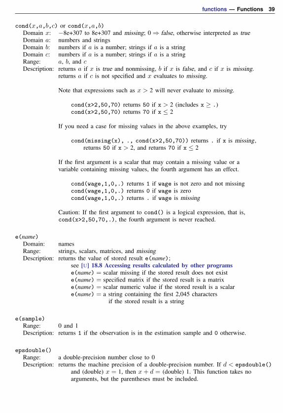
cond(x,a,b,c) or cond(x,a,b)Domain x: −8e+307 to 8e+307 and missing; 0⇒ false, otherwise interpreted as trueDomain a: numbers and stringsDomain b: numbers if a is a number; strings if a is a stringDomain c: numbers if a is a number; strings if a is a stringRange: a, b, and cDescription: returns a if x is true and nonmissing, b if x is false, and c if x is missing.
returns a if c is not specified and x evaluates to missing.
Note that expressions such as x > 2 will never evaluate to missing.
cond(x>2,50,70) returns 50 if x > 2 (includes x ≥ .)cond(x>2,50,70) returns 70 if x ≤ 2
If you need a case for missing values in the above examples, try
cond(missing(x), ., cond(x>2,50,70)) returns . if x is missing ,returns 50 if x > 2, and returns 70 if x ≤ 2
If the first argument is a scalar that may contain a missing value or avariable containing missing values, the fourth argument has an effect.
cond(wage,1,0,.) returns 1 if wage is not zero and not missingcond(wage,1,0,.) returns 0 if wage is zerocond(wage,1,0,.) returns . if wage is missing
Caution: If the first argument to cond() is a logical expression, that is,cond(x>2,50,70,.), the fourth argument is never reached.
e(name)Domain: namesRange: strings, scalars, matrices, and missingDescription: returns the value of stored result e(name);
see [U] 18.8 Accessing results calculated by other programse(name) = scalar missing if the stored result does not existe(name) = specified matrix if the stored result is a matrixe(name) = scalar numeric value if the stored result is a scalare(name) = a string containing the first 2,045 characters
if the stored result is a string
e(sample)Range: 0 and 1Description: returns 1 if the observation is in the estimation sample and 0 otherwise.
epsdouble()Range: a double-precision number close to 0Description: returns the machine precision of a double-precision number. If d < epsdouble()
and (double) x = 1, then x+ d = (double) 1. This function takes noarguments, but the parentheses must be included.
40 functions — Functions
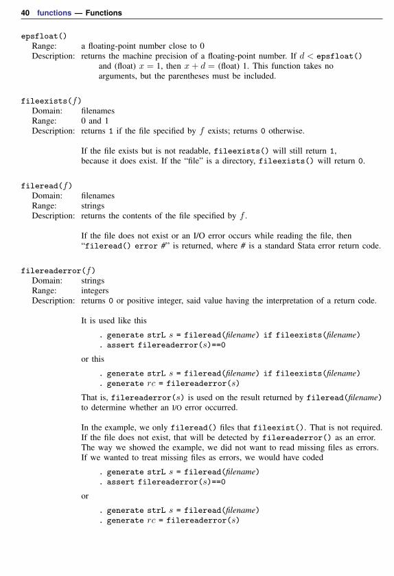
epsfloat()Range: a floating-point number close to 0Description: returns the machine precision of a floating-point number. If d < epsfloat()
and (float) x = 1, then x+ d = (float) 1. This function takes noarguments, but the parentheses must be included.
fileexists(f)Domain: filenamesRange: 0 and 1Description: returns 1 if the file specified by f exists; returns 0 otherwise.
If the file exists but is not readable, fileexists() will still return 1,because it does exist. If the “file” is a directory, fileexists() will return 0.
fileread(f)Domain: filenamesRange: stringsDescription: returns the contents of the file specified by f .
If the file does not exist or an I/O error occurs while reading the file, then“fileread() error #” is returned, where # is a standard Stata error return code.
filereaderror(f)Domain: stringsRange: integersDescription: returns 0 or positive integer, said value having the interpretation of a return code.
It is used like this
. generate strL s = fileread(filename) if fileexists(filename)
. assert filereaderror(s)==0
or this
. generate strL s = fileread(filename) if fileexists(filename)
. generate rc = filereaderror(s)
That is, filereaderror(s) is used on the result returned by fileread(filename)to determine whether an I/O error occurred.
In the example, we only fileread() files that fileexist(). That is not required.If the file does not exist, that will be detected by filereaderror() as an error.The way we showed the example, we did not want to read missing files as errors.If we wanted to treat missing files as errors, we would have coded
. generate strL s = fileread(filename)
. assert filereaderror(s)==0
or
. generate strL s = fileread(filename)
. generate rc = filereaderror(s)
functions — Functions 41
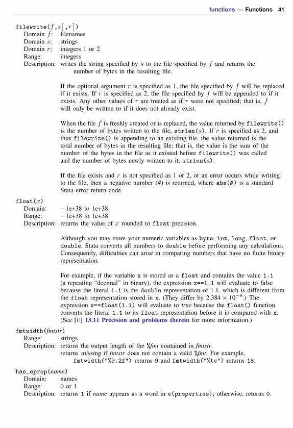
filewrite(f,s[,r])
Domain f : filenamesDomain s: stringsDomain r: integers 1 or 2Range: integersDescription: writes the string specified by s to the file specified by f and returns the
number of bytes in the resulting file.
If the optional argument r is specified as 1, the file specified by f will be replacedif it exists. If r is specified as 2, the file specified by f will be appended to if itexists. Any other values of r are treated as if r were not specified; that is, fwill only be written to if it does not already exist.
When the file f is freshly created or is replaced, the value returned by filewrite()is the number of bytes written to the file, strlen(s). If r is specified as 2, andthus filewrite() is appending to an existing file, the value returned is thetotal number of bytes in the resulting file; that is, the value is the sum of thenumber of the bytes in the file as it existed before filewrite() was calledand the number of bytes newly written to it, strlen(s).
If the file exists and r is not specified as 1 or 2, or an error occurs while writingto the file, then a negative number (#) is returned, where abs(#) is a standardStata error return code.
float(x)Domain: −1e+38 to 1e+38Range: −1e+38 to 1e+38Description: returns the value of x rounded to float precision.
Although you may store your numeric variables as byte, int, long, float, ordouble, Stata converts all numbers to double before performing any calculations.Consequently, difficulties can arise in comparing numbers that have no finite binaryrepresentation.
For example, if the variable x is stored as a float and contains the value 1.1(a repeating “decimal” in binary), the expression x==1.1 will evaluate to falsebecause the literal 1.1 is the double representation of 1.1, which is different fromthe float representation stored in x. (They differ by 2.384× 10⁻⁸.) Theexpression x==float(1.1) will evaluate to true because the float() functionconverts the literal 1.1 to its float representation before it is compared with x.(See [U] 13.11 Precision and problems therein for more information.)
fmtwidth(fmtstr)Range: stringsDescription: returns the output length of the %fmt contained in fmtstr.
returns missing if fmtstr does not contain a valid %fmt. For example,fmtwidth("%9.2f") returns 9 and fmtwidth("%tc") returns 18.
has eprop(name)Domain: namesRange: 0 or 1Description: returns 1 if name appears as a word in e(properties); otherwise, returns 0.
42 functions — Functions
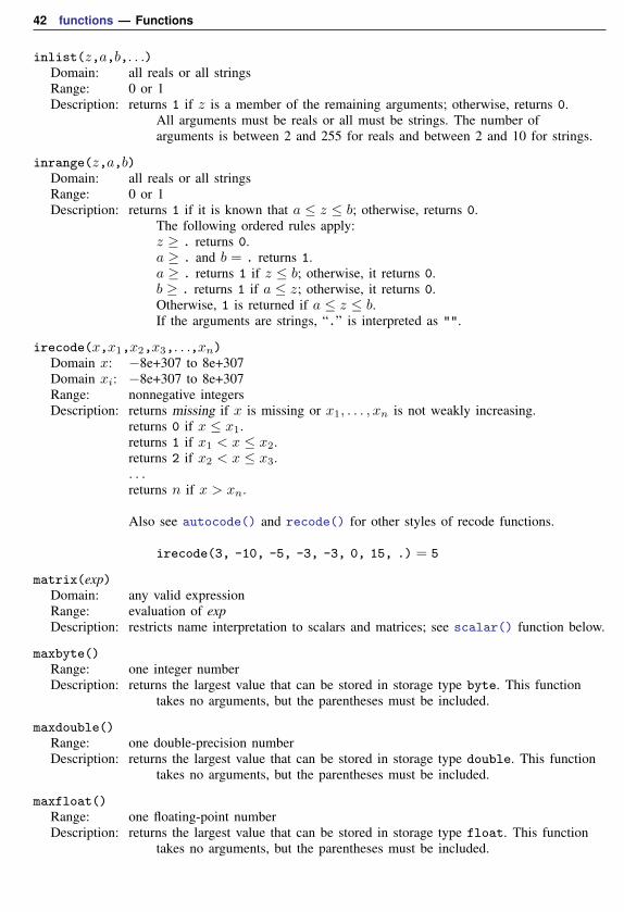
inlist(z,a,b,. . .)Domain: all reals or all stringsRange: 0 or 1Description: returns 1 if z is a member of the remaining arguments; otherwise, returns 0.
All arguments must be reals or all must be strings. The number ofarguments is between 2 and 255 for reals and between 2 and 10 for strings.
inrange(z,a,b)Domain: all reals or all stringsRange: 0 or 1Description: returns 1 if it is known that a ≤ z ≤ b; otherwise, returns 0.
The following ordered rules apply:z ≥ . returns 0.a ≥ . and b = . returns 1.a ≥ . returns 1 if z ≤ b; otherwise, it returns 0.b ≥ . returns 1 if a ≤ z; otherwise, it returns 0.Otherwise, 1 is returned if a ≤ z ≤ b.If the arguments are strings, “.” is interpreted as "".
irecode(x,x1,x2,x3,. . .,xn)Domain x: −8e+307 to 8e+307Domain xi: −8e+307 to 8e+307Range: nonnegative integersDescription: returns missing if x is missing or x1, . . . , xn is not weakly increasing.
returns 0 if x ≤ x1.returns 1 if x1 < x ≤ x2.returns 2 if x2 < x ≤ x3.. . .returns n if x > xn.
Also see autocode() and recode() for other styles of recode functions.
irecode(3, -10, -5, -3, -3, 0, 15, .) = 5
matrix(exp)Domain: any valid expressionRange: evaluation of expDescription: restricts name interpretation to scalars and matrices; see scalar() function below.
maxbyte()Range: one integer numberDescription: returns the largest value that can be stored in storage type byte. This function
takes no arguments, but the parentheses must be included.
maxdouble()Range: one double-precision numberDescription: returns the largest value that can be stored in storage type double. This function
takes no arguments, but the parentheses must be included.
maxfloat()Range: one floating-point numberDescription: returns the largest value that can be stored in storage type float. This function
takes no arguments, but the parentheses must be included.
functions — Functions 43
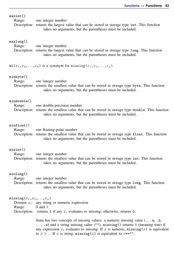
maxint()Range: one integer numberDescription: returns the largest value that can be stored in storage type int. This function
takes no arguments, but the parentheses must be included.
maxlong()Range: one integer numberDescription: returns the largest value that can be stored in storage type long. This function
takes no arguments, but the parentheses must be included.
mi(x1,x2,. . .,xn) is a synonym for missing(x1,x2,. . .,xn).
minbyte()Range: one integer numberDescription: returns the smallest value that can be stored in storage type byte. This function
takes no arguments, but the parentheses must be included.
mindouble()Range: one double-precision numberDescription: returns the smallest value that can be stored in storage type double. This function
takes no arguments, but the parentheses must be included.
minfloat()Range: one floating-point numberDescription: returns the smallest value that can be stored in storage type float. This function
takes no arguments, but the parentheses must be included.
minint()Range: one integer numberDescription: returns the smallest value that can be stored in storage type int. This function
takes no arguments, but the parentheses must be included.
minlong()Range: one integer numberDescription: returns the smallest value that can be stored in storage type long. This function
takes no arguments, but the parentheses must be included.
missing(x1,x2,. . .,xn)Domain xi: any string or numeric expressionRange: 0 and 1Description: returns 1 if any xi evaluates to missing; otherwise, returns 0.
Stata has two concepts of missing values: a numeric missing value (., .a, .b,. . . , .z) and a string missing value (""). missing() returns 1 (meaning true) ifany expression xi evaluates to missing. If x is numeric, missing(x) is equivalentto x ≥ .. If x is string, missing(x) is equivalent to x=="".
44 functions — Functions
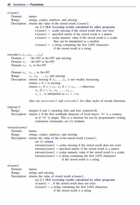
r(name)Domain: namesRange: strings, scalars, matrices, and missingDescription: returns the value of the stored result r(name);
see [U] 18.8 Accessing results calculated by other programsr(name) = scalar missing if the stored result does not existr(name) = specified matrix if the stored result is a matrixr(name) = scalar numeric value if the stored result is a scalar
that can be interpreted as a numberr(name) = a string containing the first 2,045 characters
if the stored result is a string
recode(x,x1,x2,. . .,xn)Domain x: −8e+307 to 8e+307 and missingDomain x1: −8e+307 to 8e+307Domain x2: x1 to 8e+307. . .Domain xn: xn−1 to 8e+307Range: x1, x2, . . ., xn and missingDescription: returns missing if x1, . . . , xn is not weakly increasing.
returns x if x is missing.returns x1 if x ≤ x1; x2 if x ≤ x2, . . .; otherwise,
xn if x > x1, x2, . . . , xn−1.xi ≥ . is interpreted as xi = +∞.
Also see autocode() and irecode() for other styles of recode functions.
replay()Range: integers 0 and 1, meaning false and true, respectivelyDescription: returns 1 if the first nonblank character of local macro ‘0’ is a comma,
or if ‘0’ is empty. This is a function for use by programmers writingestimation commands; see [P] ereturn.
return(name)Domain: namesRange: strings, scalars, matrices, and missingDescription: returns the value of the to-be-stored result r(name);
see [P] return.return(name) = scalar missing if the stored result does not existreturn(name) = specified matrix if the stored result is a matrixreturn(name) = scalar numeric value if the stored result is a scalarreturn(name) = a string containing the first 2,045 characters
if the stored result is a string
s(name)Domain: namesRange: strings and missingDescription: returns the value of stored result s(name);
see [U] 18.8 Accessing results calculated by other programss(name) = . if the stored result does not exists(name) = a string containing the first 2,045 characters
if the stored result is a string
functions — Functions 45
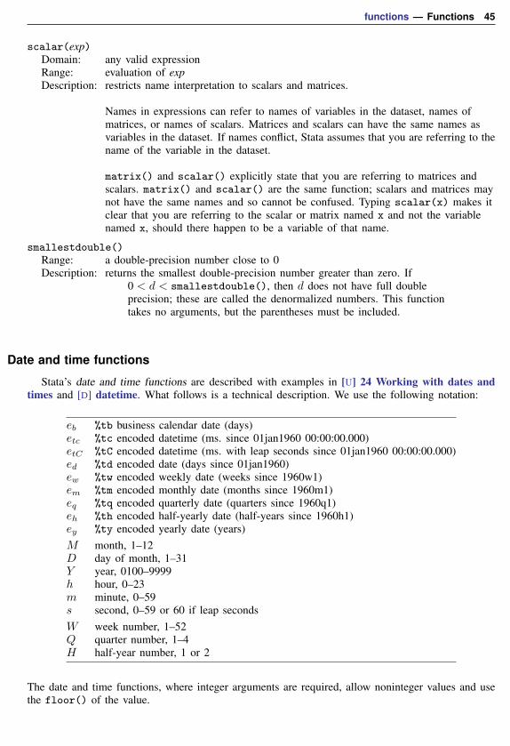
scalar(exp)Domain: any valid expressionRange: evaluation of expDescription: restricts name interpretation to scalars and matrices.
Names in expressions can refer to names of variables in the dataset, names ofmatrices, or names of scalars. Matrices and scalars can have the same names asvariables in the dataset. If names conflict, Stata assumes that you are referring to thename of the variable in the dataset.
matrix() and scalar() explicitly state that you are referring to matrices andscalars. matrix() and scalar() are the same function; scalars and matrices maynot have the same names and so cannot be confused. Typing scalar(x) makes itclear that you are referring to the scalar or matrix named x and not the variablenamed x, should there happen to be a variable of that name.
smallestdouble()Range: a double-precision number close to 0Description: returns the smallest double-precision number greater than zero. If
0 < d < smallestdouble(), then d does not have full doubleprecision; these are called the denormalized numbers. This functiontakes no arguments, but the parentheses must be included.
Date and time functions
Stata’s date and time functions are described with examples in [U] 24 Working with dates andtimes and [D] datetime. What follows is a technical description. We use the following notation:
eb %tb business calendar date (days)etc %tc encoded datetime (ms. since 01jan1960 00:00:00.000)etC %tC encoded datetime (ms. with leap seconds since 01jan1960 00:00:00.000)ed %td encoded date (days since 01jan1960)ew %tw encoded weekly date (weeks since 1960w1)em %tm encoded monthly date (months since 1960m1)eq %tq encoded quarterly date (quarters since 1960q1)eh %th encoded half-yearly date (half-years since 1960h1)ey %ty encoded yearly date (years)M month, 1–12D day of month, 1–31Y year, 0100–9999h hour, 0–23m minute, 0–59s second, 0–59 or 60 if leap secondsW week number, 1–52Q quarter number, 1–4H half-year number, 1 or 2
The date and time functions, where integer arguments are required, allow noninteger values and usethe floor() of the value.
46 functions — Functions
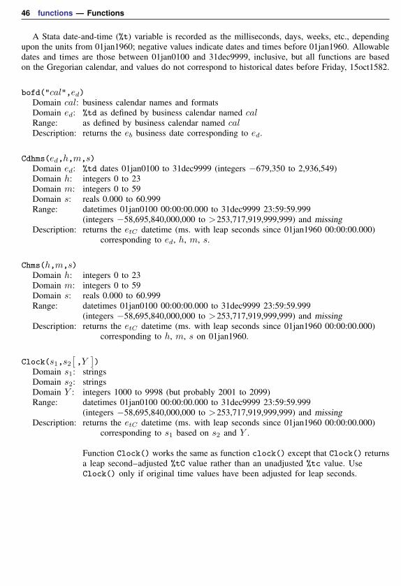
A Stata date-and-time (%t) variable is recorded as the milliseconds, days, weeks, etc., dependingupon the units from 01jan1960; negative values indicate dates and times before 01jan1960. Allowabledates and times are those between 01jan0100 and 31dec9999, inclusive, but all functions are basedon the Gregorian calendar, and values do not correspond to historical dates before Friday, 15oct1582.
bofd("cal",ed)Domain cal: business calendar names and formatsDomain ed: %td as defined by business calendar named calRange: as defined by business calendar named calDescription: returns the eb business date corresponding to ed.
Cdhms(ed,h,m,s)Domain ed: %td dates 01jan0100 to 31dec9999 (integers −679,350 to 2,936,549)Domain h: integers 0 to 23Domain m: integers 0 to 59Domain s: reals 0.000 to 60.999Range: datetimes 01jan0100 00:00:00.000 to 31dec9999 23:59:59.999
(integers −58,695,840,000,000 to >253,717,919,999,999) and missingDescription: returns the etC datetime (ms. with leap seconds since 01jan1960 00:00:00.000)
corresponding to ed, h, m, s.
Chms(h,m,s)Domain h: integers 0 to 23Domain m: integers 0 to 59Domain s: reals 0.000 to 60.999Range: datetimes 01jan0100 00:00:00.000 to 31dec9999 23:59:59.999
(integers −58,695,840,000,000 to >253,717,919,999,999) and missingDescription: returns the etC datetime (ms. with leap seconds since 01jan1960 00:00:00.000)
corresponding to h, m, s on 01jan1960.
Clock(s1,s2[,Y])
Domain s1: stringsDomain s2: stringsDomain Y : integers 1000 to 9998 (but probably 2001 to 2099)Range: datetimes 01jan0100 00:00:00.000 to 31dec9999 23:59:59.999
(integers −58,695,840,000,000 to >253,717,919,999,999) and missingDescription: returns the etC datetime (ms. with leap seconds since 01jan1960 00:00:00.000)
corresponding to s1 based on s2 and Y .
Function Clock() works the same as function clock() except that Clock() returnsa leap second–adjusted %tC value rather than an unadjusted %tc value. UseClock() only if original time values have been adjusted for leap seconds.
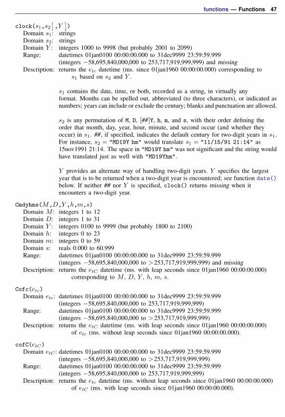
functions — Functions 47
clock(s1,s2[,Y])
Domain s1: stringsDomain s2: stringsDomain Y : integers 1000 to 9998 (but probably 2001 to 2099)Range: datetimes 01jan0100 00:00:00.000 to 31dec9999 23:59:59.999
(integers −58,695,840,000,000 to 253,717,919,999,999) and missingDescription: returns the etc datetime (ms. since 01jan1960 00:00:00.000) corresponding to
s1 based on s2 and Y .
s1 contains the date, time, or both, recorded as a string, in virtually anyformat. Months can be spelled out, abbreviated (to three characters), or indicated asnumbers; years can include or exclude the century; blanks and punctuation are allowed.
s2 is any permutation of M, D, [##]Y, h, m, and s, with their order defining theorder that month, day, year, hour, minute, and second occur (and whether theyoccur) in s1. ##, if specified, indicates the default century for two-digit years in s1.For instance, s2 = "MD19Y hm" would translate s1 = "11/15/91 21:14" as15nov1991 21:14. The space in "MD19Y hm" was not significant and the string wouldhave translated just as well with "MD19Yhm".
Y provides an alternate way of handling two-digit years. Y specifies the largestyear that is to be returned when a two-digit year is encountered; see function date()below. If neither ## nor Y is specified, clock() returns missing when itencounters a two-digit year.
Cmdyhms(M,D,Y ,h,m,s)Domain M : integers 1 to 12Domain D: integers 1 to 31Domain Y : integers 0100 to 9999 (but probably 1800 to 2100)Domain h: integers 0 to 23Domain m: integers 0 to 59Domain s: reals 0.000 to 60.999Range: datetimes 01jan0100 00:00:00.000 to 31dec9999 23:59:59.999
(integers −58,695,840,000,000 to >253,717,919,999,999) and missingDescription: returns the etC datetime (ms. with leap seconds since 01jan1960 00:00:00.000)
corresponding to M , D, Y , h, m, s.
Cofc(etc)Domain etc: datetimes 01jan0100 00:00:00.000 to 31dec9999 23:59:59.999
(integers −58,695,840,000,000 to 253,717,919,999,999)Range: datetimes 01jan0100 00:00:00.000 to 31dec9999 23:59:59.999
(integers −58,695,840,000,000 to >253,717,919,999,999)Description: returns the etC datetime (ms. with leap seconds since 01jan1960 00:00:00.000)
of etc (ms. without leap seconds since 01jan1960 00:00:00.000).
cofC(etC)Domain etC : datetimes 01jan0100 00:00:00.000 to 31dec9999 23:59:59.999
(integers −58,695,840,000,000 to >253,717,919,999,999)Range: datetimes 01jan0100 00:00:00.000 to 31dec9999 23:59:59.999
(integers −58,695,840,000,000 to 253,717,919,999,999)Description: returns the etc datetime (ms. without leap seconds since 01jan1960 00:00:00.000)
of etC (ms. with leap seconds since 01jan1960 00:00:00.000).
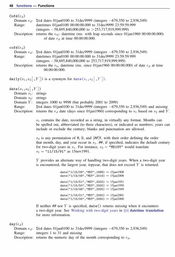
48 functions — Functions
Cofd(ed)Domain ed: %td dates 01jan0100 to 31dec9999 (integers −679,350 to 2,936,549)Range: datetimes 01jan0100 00:00:00.000 to 31dec9999 23:59:59.999
(integers −58,695,840,000,000 to >253,717,919,999,999)Description: returns the etC datetime (ms. with leap seconds since 01jan1960 00:00:00.000)
of date ed at time 00:00:00.000.
cofd(ed)Domain ed: %td dates 01jan0100 to 31dec9999 (integers −679,350 to 2,936,549)Range: datetimes 01jan0100 00:00:00.000 to 31dec9999 23:59:59.999
(integers −58,695,840,000,000 to 253,717,919,999,999)Description: returns the etc datetime (ms. since 01jan1960 00:00:00.000) of date ed at time
00:00:00.000.
daily(s1,s2[,Y]) is a synonym for date(s1,s2
[,Y]).
date(s1,s2[,Y])
Domain s1: stringsDomain s2: stringsDomain Y : integers 1000 to 9998 (but probably 2001 to 2099)Range: %td dates 01jan0100 to 31dec9999 (integers −679,350 to 2,936,549) and missingDescription: returns the ed date (days since 01jan1960) corresponding to s1 based on s2 and Y .
s1 contains the date, recorded as a string, in virtually any format. Months canbe spelled out, abbreviated (to three characters), or indicated as numbers; years caninclude or exclude the century; blanks and punctuation are allowed.
s2 is any permutation of M, D, and [##]Y, with their order defining the orderthat month, day, and year occur in s1. ##, if specified, indicates the default centuryfor two-digit years in s1. For instance, s2 = "MD19Y" would translates1 = "11/15/91" as 15nov1991.
Y provides an alternate way of handling two-digit years. When a two-digit yearis encountered, the largest year, topyear, that does not exceed Y is returned.
date("1/15/08","MDY",1999) = 15jan1908date("1/15/08","MDY",2019) = 15jan2008
date("1/15/51","MDY",2000) = 15jan1951date("1/15/50","MDY",2000) = 15jan1950date("1/15/49","MDY",2000) = 15jan1949
date("1/15/01","MDY",2050) = 15jan2001date("1/15/00","MDY",2050) = 15jan2000
If neither ## nor Y is specified, date() returns missing when it encountersa two-digit year. See Working with two-digit years in [D] datetime translationfor more information.
day(ed)Domain ed: %td dates 01jan0100 to 31dec9999 (integers −679,350 to 2,936,549)Range: integers 1 to 31 and missingDescription: returns the numeric day of the month corresponding to ed.
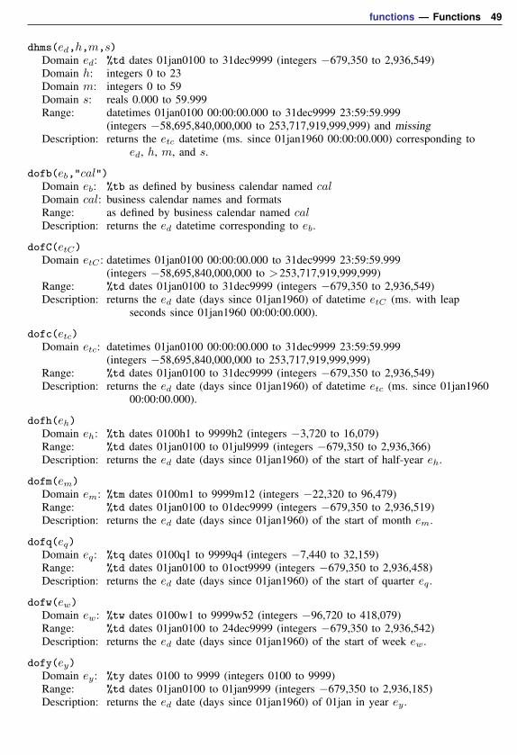
functions — Functions 49
dhms(ed,h,m,s)Domain ed: %td dates 01jan0100 to 31dec9999 (integers −679,350 to 2,936,549)Domain h: integers 0 to 23Domain m: integers 0 to 59Domain s: reals 0.000 to 59.999Range: datetimes 01jan0100 00:00:00.000 to 31dec9999 23:59:59.999
(integers −58,695,840,000,000 to 253,717,919,999,999) and missingDescription: returns the etc datetime (ms. since 01jan1960 00:00:00.000) corresponding to
ed, h, m, and s.
dofb(eb,"cal")Domain eb: %tb as defined by business calendar named calDomain cal: business calendar names and formatsRange: as defined by business calendar named calDescription: returns the ed datetime corresponding to eb.
dofC(etC)Domain etC : datetimes 01jan0100 00:00:00.000 to 31dec9999 23:59:59.999
(integers −58,695,840,000,000 to >253,717,919,999,999)Range: %td dates 01jan0100 to 31dec9999 (integers −679,350 to 2,936,549)Description: returns the ed date (days since 01jan1960) of datetime etC (ms. with leap
seconds since 01jan1960 00:00:00.000).
dofc(etc)Domain etc: datetimes 01jan0100 00:00:00.000 to 31dec9999 23:59:59.999
(integers −58,695,840,000,000 to 253,717,919,999,999)Range: %td dates 01jan0100 to 31dec9999 (integers −679,350 to 2,936,549)Description: returns the ed date (days since 01jan1960) of datetime etc (ms. since 01jan1960
00:00:00.000).
dofh(eh)Domain eh: %th dates 0100h1 to 9999h2 (integers −3,720 to 16,079)Range: %td dates 01jan0100 to 01jul9999 (integers −679,350 to 2,936,366)Description: returns the ed date (days since 01jan1960) of the start of half-year eh.
dofm(em)Domain em: %tm dates 0100m1 to 9999m12 (integers −22,320 to 96,479)Range: %td dates 01jan0100 to 01dec9999 (integers −679,350 to 2,936,519)Description: returns the ed date (days since 01jan1960) of the start of month em.
dofq(eq)Domain eq: %tq dates 0100q1 to 9999q4 (integers −7,440 to 32,159)Range: %td dates 01jan0100 to 01oct9999 (integers −679,350 to 2,936,458)Description: returns the ed date (days since 01jan1960) of the start of quarter eq .
dofw(ew)Domain ew: %tw dates 0100w1 to 9999w52 (integers −96,720 to 418,079)Range: %td dates 01jan0100 to 24dec9999 (integers −679,350 to 2,936,542)Description: returns the ed date (days since 01jan1960) of the start of week ew.
dofy(ey)Domain ey: %ty dates 0100 to 9999 (integers 0100 to 9999)Range: %td dates 01jan0100 to 01jan9999 (integers −679,350 to 2,936,185)Description: returns the ed date (days since 01jan1960) of 01jan in year ey .
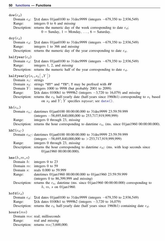
50 functions — Functions
dow(ed)Domain ed: %td dates 01jan0100 to 31dec9999 (integers −679,350 to 2,936,549)Range: integers 0 to 6 and missingDescription: returns the numeric day of the week corresponding to date ed;
0 = Sunday, 1 = Monday, . . . , 6 = Saturday.
doy(ed)Domain ed: %td dates 01jan0100 to 31dec9999 (integers −679,350 to 2,936,549)Range: integers 1 to 366 and missingDescription: returns the numeric day of the year corresponding to date ed.
halfyear(ed)Domain ed: %td dates 01jan0100 to 31dec9999 (integers −679,350 to 2,936,549)Range: integers 1, 2, and missingDescription: returns the numeric half of the year corresponding to date ed.
halfyearly(s1,s2[,Y])
Domain s1: stringsDomain s2: strings "HY" and "YH"; Y may be prefixed with ##Domain Y : integers 1000 to 9998 (but probably 2001 to 2099)Range: %th dates 0100h1 to 9999h2 (integers −3,720 to 16,079) and missingDescription: returns the eh half-yearly date (half-years since 1960h1) corresponding to s1 based
on s2 and Y ; Y specifies topyear; see date().
hh(etc)Domain etc: datetimes 01jan0100 00:00:00.000 to 31dec9999 23:59:59.999
(integers −58,695,840,000,000 to 253,717,919,999,999)Range: integers 0 through 23, missingDescription: returns the hour corresponding to datetime etc (ms. since 01jan1960 00:00:00.000).
hhC(etC)Domain etC : datetimes 01jan0100 00:00:00.000 to 31dec9999 23:59:59.999
(integers −58,695,840,000,000 to >253,717,919,999,999)Range: integers 0 through 23, missingDescription: returns the hour corresponding to datetime etC (ms. with leap seconds since
01jan1960 00:00:00.000).
hms(h,m,s)Domain h: integers 0 to 23Domain m: integers 0 to 59Domain s: reals 0.000 to 59.999Range: datetimes 01jan1960 00:00:00.000 to 01jan1960 23:59:59.999
(integers 0 to 86,399,999 and missing)Description: returns the etc datetime (ms. since 01jan1960 00:00:00.000) corresponding to
h, m, s on 01jan1960.
hofd(ed)Domain ed: %td dates 01jan0100 to 31dec9999 (integers −679,350 to 2,936,549)Range: %th dates 0100h1 to 9999h2 (integers −3,720 to 16,079)Description: returns the eh half-yearly date (half years since 1960h1) containing date ed.
hours(ms)Domain ms: real; millisecondsRange: real and missingDescription: returns ms/3,600,000.
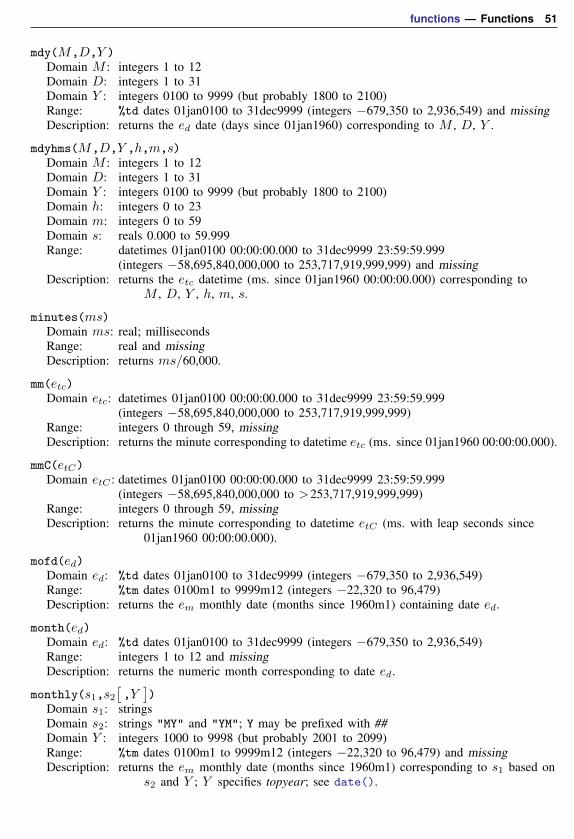
functions — Functions 51
mdy(M,D,Y )Domain M : integers 1 to 12Domain D: integers 1 to 31Domain Y : integers 0100 to 9999 (but probably 1800 to 2100)Range: %td dates 01jan0100 to 31dec9999 (integers −679,350 to 2,936,549) and missingDescription: returns the ed date (days since 01jan1960) corresponding to M , D, Y .
mdyhms(M,D,Y ,h,m,s)Domain M : integers 1 to 12Domain D: integers 1 to 31Domain Y : integers 0100 to 9999 (but probably 1800 to 2100)Domain h: integers 0 to 23Domain m: integers 0 to 59Domain s: reals 0.000 to 59.999Range: datetimes 01jan0100 00:00:00.000 to 31dec9999 23:59:59.999
(integers −58,695,840,000,000 to 253,717,919,999,999) and missingDescription: returns the etc datetime (ms. since 01jan1960 00:00:00.000) corresponding to
M , D, Y , h, m, s.
minutes(ms)Domain ms: real; millisecondsRange: real and missingDescription: returns ms/60,000.
mm(etc)Domain etc: datetimes 01jan0100 00:00:00.000 to 31dec9999 23:59:59.999
(integers −58,695,840,000,000 to 253,717,919,999,999)Range: integers 0 through 59, missingDescription: returns the minute corresponding to datetime etc (ms. since 01jan1960 00:00:00.000).
mmC(etC)Domain etC : datetimes 01jan0100 00:00:00.000 to 31dec9999 23:59:59.999
(integers −58,695,840,000,000 to >253,717,919,999,999)Range: integers 0 through 59, missingDescription: returns the minute corresponding to datetime etC (ms. with leap seconds since
01jan1960 00:00:00.000).
mofd(ed)Domain ed: %td dates 01jan0100 to 31dec9999 (integers −679,350 to 2,936,549)Range: %tm dates 0100m1 to 9999m12 (integers −22,320 to 96,479)Description: returns the em monthly date (months since 1960m1) containing date ed.
month(ed)Domain ed: %td dates 01jan0100 to 31dec9999 (integers −679,350 to 2,936,549)Range: integers 1 to 12 and missingDescription: returns the numeric month corresponding to date ed.
monthly(s1,s2[,Y])
Domain s1: stringsDomain s2: strings "MY" and "YM"; Y may be prefixed with ##Domain Y : integers 1000 to 9998 (but probably 2001 to 2099)Range: %tm dates 0100m1 to 9999m12 (integers −22,320 to 96,479) and missingDescription: returns the em monthly date (months since 1960m1) corresponding to s1 based on
s2 and Y ; Y specifies topyear; see date().
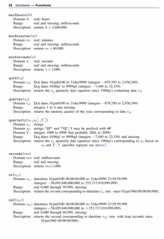
52 functions — Functions
msofhours(h)Domain h: real; hoursRange: real and missing; millisecondsDescription: returns h× 3,600,000.
msofminutes(m)Domain m: real; minutesRange: real and missing; millisecondsDescription: returns m× 60,000.
msofseconds(s)Domain s: real; secondsRange: real and missing; millisecondsDescription: returns s× 1,000.
qofd(ed)Domain ed: %td dates 01jan0100 to 31dec9999 (integers −679,350 to 2,936,549)Range: %tq dates 0100q1 to 9999q4 (integers −7,440 to 32,159)Description: returns the eq quarterly date (quarters since 1960q1) containing date ed.
quarter(ed)Domain ed: %td dates 01jan0100 to 31dec9999 (integers −679,350 to 2,936,549)Range: integers 1 to 4 and missingDescription: returns the numeric quarter of the year corresponding to date ed.
quarterly(s1,s2[,Y])
Domain s1: stringsDomain s2: strings "QY" and "YQ"; Y may be prefixed with ##Domain Y : integers 1000 to 9998 (but probably 2001 to 2099)Range: %tq dates 0100q1 to 9999q4 (integers −7,440 to 32,159) and missingDescription: returns the eq quarterly date (quarters since 1960q1) corresponding to s1 based on
s2 and Y ; Y specifies topyear; see date().
seconds(ms)Domain ms: real; millisecondsRange: real and missingDescription: returns ms/1,000.
ss(etc)Domain etc: datetimes 01jan0100 00:00:00.000 to 31dec9999 23:59:59.999
(integers −58,695,840,000,000 to 253,717,919,999,999)Range: real 0.000 through 59.999, missingDescription: returns the second corresponding to datetime etc (ms. since 01jan1960 00:00:00.000).
ssC(etC)Domain etC : datetimes 01jan0100 00:00:00.000 to 31dec9999 23:59:59.999
(integers −58,695,840,000,000 to >253,717,919,999,999)Range: real 0.000 through 60.999, missingDescription: returns the second corresponding to datetime etC (ms. with leap seconds since
01jan1960 00:00:00.000).
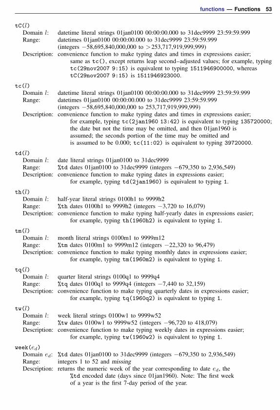
functions — Functions 53
tC(l)Domain l: datetime literal strings 01jan0100 00:00:00.000 to 31dec9999 23:59:59.999Range: datetimes 01jan0100 00:00:00.000 to 31dec9999 23:59:59.999
(integers −58,695,840,000,000 to >253,717,919,999,999)Description: convenience function to make typing dates and times in expressions easier;
same as tc(), except returns leap second–adjusted values; for example, typingtc(29nov2007 9:15) is equivalent to typing 1511946900000, whereastC(29nov2007 9:15) is 1511946923000.
tc(l)Domain l: datetime literal strings 01jan0100 00:00:00.000 to 31dec9999 23:59:59.999Range: datetimes 01jan0100 00:00:00.000 to 31dec9999 23:59:59.999
(integers −58,695,840,000,000 to 253,717,919,999,999)Description: convenience function to make typing dates and times in expressions easier;
for example, typing tc(2jan1960 13:42) is equivalent to typing 135720000;the date but not the time may be omitted, and then 01jan1960 isassumed; the seconds portion of the time may be omitted andis assumed to be 0.000; tc(11:02) is equivalent to typing 39720000.
td(l)Domain l: date literal strings 01jan0100 to 31dec9999Range: %td dates 01jan0100 to 31dec9999 (integers −679,350 to 2,936,549)Description: convenience function to make typing dates in expressions easier;
for example, typing td(2jan1960) is equivalent to typing 1.
th(l)Domain l: half-year literal strings 0100h1 to 9999h2Range: %th dates 0100h1 to 9999h2 (integers −3,720 to 16,079)Description: convenience function to make typing half-yearly dates in expressions easier;
for example, typing th(1960h2) is equivalent to typing 1.
tm(l)Domain l: month literal strings 0100m1 to 9999m12Range: %tm dates 0100m1 to 9999m12 (integers −22,320 to 96,479)Description: convenience function to make typing monthly dates in expressions easier;
for example, typing tm(1960m2) is equivalent to typing 1.
tq(l)Domain l: quarter literal strings 0100q1 to 9999q4Range: %tq dates 0100q1 to 9999q4 (integers −7,440 to 32,159)Description: convenience function to make typing quarterly dates in expressions easier;
for example, typing tq(1960q2) is equivalent to typing 1.
tw(l)Domain l: week literal strings 0100w1 to 9999w52Range: %tw dates 0100w1 to 9999w52 (integers −96,720 to 418,079)Description: convenience function to make typing weekly dates in expressions easier;
for example, typing tw(1960w2) is equivalent to typing 1.
week(ed)Domain ed: %td dates 01jan0100 to 31dec9999 (integers −679,350 to 2,936,549)Range: integers 1 to 52 and missingDescription: returns the numeric week of the year corresponding to date ed, the
%td encoded date (days since 01jan1960). Note: The first weekof a year is the first 7-day period of the year.
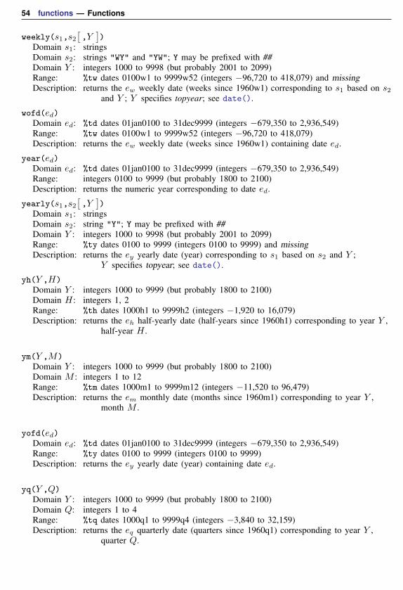
54 functions — Functions
weekly(s1,s2[,Y])
Domain s1: stringsDomain s2: strings "WY" and "YW"; Y may be prefixed with ##Domain Y : integers 1000 to 9998 (but probably 2001 to 2099)Range: %tw dates 0100w1 to 9999w52 (integers −96,720 to 418,079) and missingDescription: returns the ew weekly date (weeks since 1960w1) corresponding to s1 based on s2
and Y ; Y specifies topyear; see date().
wofd(ed)Domain ed: %td dates 01jan0100 to 31dec9999 (integers −679,350 to 2,936,549)Range: %tw dates 0100w1 to 9999w52 (integers −96,720 to 418,079)Description: returns the ew weekly date (weeks since 1960w1) containing date ed.
year(ed)Domain ed: %td dates 01jan0100 to 31dec9999 (integers −679,350 to 2,936,549)Range: integers 0100 to 9999 (but probably 1800 to 2100)Description: returns the numeric year corresponding to date ed.
yearly(s1,s2[,Y])
Domain s1: stringsDomain s2: string "Y"; Y may be prefixed with ##Domain Y : integers 1000 to 9998 (but probably 2001 to 2099)Range: %ty dates 0100 to 9999 (integers 0100 to 9999) and missingDescription: returns the ey yearly date (year) corresponding to s1 based on s2 and Y ;
Y specifies topyear; see date().
yh(Y ,H)Domain Y : integers 1000 to 9999 (but probably 1800 to 2100)Domain H : integers 1, 2Range: %th dates 1000h1 to 9999h2 (integers −1,920 to 16,079)Description: returns the eh half-yearly date (half-years since 1960h1) corresponding to year Y ,
half-year H .
ym(Y ,M)Domain Y : integers 1000 to 9999 (but probably 1800 to 2100)Domain M : integers 1 to 12Range: %tm dates 1000m1 to 9999m12 (integers −11,520 to 96,479)Description: returns the em monthly date (months since 1960m1) corresponding to year Y ,
month M .
yofd(ed)Domain ed: %td dates 01jan0100 to 31dec9999 (integers −679,350 to 2,936,549)Range: %ty dates 0100 to 9999 (integers 0100 to 9999)Description: returns the ey yearly date (year) containing date ed.
yq(Y ,Q)Domain Y : integers 1000 to 9999 (but probably 1800 to 2100)Domain Q: integers 1 to 4Range: %tq dates 1000q1 to 9999q4 (integers −3,840 to 32,159)Description: returns the eq quarterly date (quarters since 1960q1) corresponding to year Y ,
quarter Q.
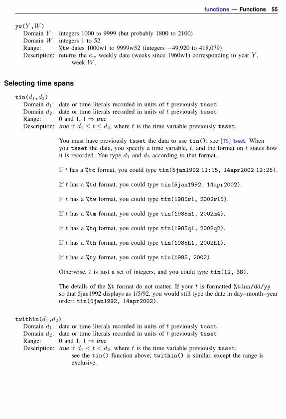
functions — Functions 55
yw(Y ,W)Domain Y : integers 1000 to 9999 (but probably 1800 to 2100)Domain W : integers 1 to 52Range: %tw dates 1000w1 to 9999w52 (integers −49,920 to 418,079)Description: returns the ew weekly date (weeks since 1960w1) corresponding to year Y ,
week W .
Selecting time spans
tin(d1,d2)Domain d1: date or time literals recorded in units of t previously tssetDomain d2: date or time literals recorded in units of t previously tssetRange: 0 and 1, 1⇒ trueDescription: true if d1 ≤ t ≤ d2, where t is the time variable previously tsset.
You must have previously tsset the data to use tin(); see [TS] tsset. Whenyou tsset the data, you specify a time variable, t, and the format on t states howit is recorded. You type d1 and d2 according to that format.
If t has a %tc format, you could type tin(5jan1992 11:15, 14apr2002 12:25).
If t has a %td format, you could type tin(5jan1992, 14apr2002).
If t has a %tw format, you could type tin(1985w1, 2002w15).
If t has a %tm format, you could type tin(1985m1, 2002m4).
If t has a %tq format, you could type tin(1985q1, 2002q2).
If t has a %th format, you could type tin(1985h1, 2002h1).
If t has a %ty format, you could type tin(1985, 2002).
Otherwise, t is just a set of integers, and you could type tin(12, 38).
The details of the %t format do not matter. If your t is formatted %tdnn/dd/yyso that 5jan1992 displays as 1/5/92, you would still type the date in day–month–yearorder: tin(5jan1992, 14apr2002).
twithin(d1,d2)Domain d1: date or time literals recorded in units of t previously tssetDomain d2: date or time literals recorded in units of t previously tssetRange: 0 and 1, 1⇒ trueDescription: true if d1 < t < d2, where t is the time variable previously tsset;
see the tin() function above; twithin() is similar, except the range isexclusive.
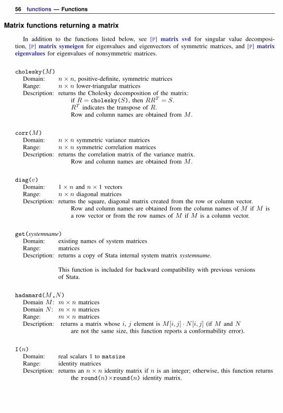
56 functions — Functions
Matrix functions returning a matrix
In addition to the functions listed below, see [P] matrix svd for singular value decomposi-tion, [P] matrix symeigen for eigenvalues and eigenvectors of symmetric matrices, and [P] matrixeigenvalues for eigenvalues of nonsymmetric matrices.
cholesky(M)Domain: n× n, positive-definite, symmetric matricesRange: n× n lower-triangular matricesDescription: returns the Cholesky decomposition of the matrix:
if R = cholesky(S), then RRT = S.RT indicates the transpose of R.Row and column names are obtained from M .
corr(M)Domain: n× n symmetric variance matricesRange: n× n symmetric correlation matricesDescription: returns the correlation matrix of the variance matrix.
Row and column names are obtained from M .
diag(v)Domain: 1× n and n× 1 vectorsRange: n× n diagonal matricesDescription: returns the square, diagonal matrix created from the row or column vector.
Row and column names are obtained from the column names of M if M isa row vector or from the row names of M if M is a column vector.
get(systemname)Domain: existing names of system matricesRange: matricesDescription: returns a copy of Stata internal system matrix systemname.
This function is included for backward compatibility with previous versionsof Stata.
hadamard(M,N)Domain M : m× n matricesDomain N : m× n matricesRange: m× n matricesDescription: returns a matrix whose i, j element is M [i, j] ·N [i, j] (if M and N
are not the same size, this function reports a conformability error).
I(n)Domain: real scalars 1 to matsizeRange: identity matricesDescription: returns an n× n identity matrix if n is an integer; otherwise, this function returns
the round(n)×round(n) identity matrix.
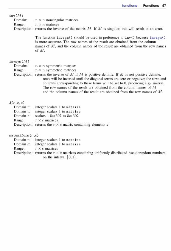
functions — Functions 57
inv(M)Domain: n× n nonsingular matricesRange: n× n matricesDescription: returns the inverse of the matrix M . If M is singular, this will result in an error.
The function invsym() should be used in preference to inv() because invsym()is more accurate. The row names of the result are obtained from the columnnames of M , and the column names of the result are obtained from the row namesof M .
invsym(M)Domain: n× n symmetric matricesRange: n× n symmetric matricesDescription: returns the inverse of M if M is positive definite. If M is not positive definite,
rows will be inverted until the diagonal terms are zero or negative; the rows andcolumns corresponding to these terms will be set to 0, producing a g2 inverse.The row names of the result are obtained from the column names of M ,and the column names of the result are obtained from the row names of M .
J(r,c,z)Domain r: integer scalars 1 to matsizeDomain c: integer scalars 1 to matsizeDomain z: scalars −8e+307 to 8e+307Range: r × c matricesDescription: returns the r × c matrix containing elements z.
matuniform(r,c)Domain r: integer scalars 1 to matsizeDomain c: integer scalars 1 to matsizeRange: r × c matricesDescription: returns the r × c matrices containing uniformly distributed pseudorandom numbers
on the interval [ 0, 1).
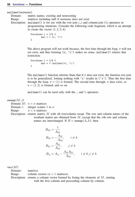
58 functions — Functions
nullmat(matname)Domain: matrix names, existing and nonexistingRange: matrices including null if matname does not existDescription: nullmat() is for use with the row-join (,) and column-join (\) operators in
programming situations. Consider the following code fragment, which is an attemptto create the vector (1, 2, 3, 4):
forvalues i = 1/4 {mat v = (v, ‘i’)
}
The above program will not work because, the first time through the loop, v will notyet exist, and thus forming (v, ‘i’) makes no sense. nullmat() relaxes thatrestriction:
forvalues i = 1/4 {mat v = (nullmat(v), ‘i’)
}
The nullmat() function informs Stata that if v does not exist, the function row-joinis to be generalized. Joining nothing with ‘i’ results in (‘i’). Thus the first timethrough the loop, v = (1) is formed. The second time through, v does exist, sov = (1, 2) is formed, and so on.
nullmat() can be used only with the , and \ operators.
sweep(M,i)Domain M : n× n matricesDomain i: integer scalars 1 to nRange: n× n matricesDescription: returns matrix M with ith row/column swept. The row and column names of the
resultant matrix are obtained from M , except that the nth row and columnnames are interchanged. If B = sweep(A,k), then
Bkk =1
Akk
Bik = −AikAkk
, i 6= k
Bkj =AkjAkk
, j 6= k
Bij = Aij −AikAkjAkk
, i 6= k, j 6= k
vec(M)Domain: matricesRange: column vectors (n× 1 matrices)Description: returns a column vector formed by listing the elements of M , starting
with the first column and proceeding column by column.
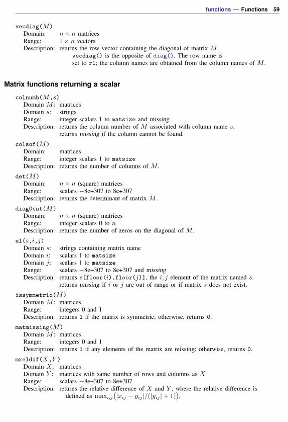
functions — Functions 59
vecdiag(M)Domain: n× n matricesRange: 1× n vectorsDescription: returns the row vector containing the diagonal of matrix M .
vecdiag() is the opposite of diag(). The row name isset to r1; the column names are obtained from the column names of M .
Matrix functions returning a scalar
colnumb(M,s)Domain M : matricesDomain s: stringsRange: integer scalars 1 to matsize and missingDescription: returns the column number of M associated with column name s.
returns missing if the column cannot be found.
colsof(M)Domain: matricesRange: integer scalars 1 to matsizeDescription: returns the number of columns of M .
det(M)Domain: n× n (square) matricesRange: scalars −8e+307 to 8e+307Description: returns the determinant of matrix M .
diag0cnt(M)Domain: n× n (square) matricesRange: integer scalars 0 to nDescription: returns the number of zeros on the diagonal of M .
el(s,i,j)Domain s: strings containing matrix nameDomain i: scalars 1 to matsizeDomain j: scalars 1 to matsizeRange: scalars −8e+307 to 8e+307 and missingDescription: returns s[floor(i),floor(j)], the i, j element of the matrix named s.
returns missing if i or j are out of range or if matrix s does not exist.
issymmetric(M)Domain M : matricesRange: integers 0 and 1Description: returns 1 if the matrix is symmetric; otherwise, returns 0.
matmissing(M)Domain M : matricesRange: integers 0 and 1Description: returns 1 if any elements of the matrix are missing; otherwise, returns 0.
mreldif(X,Y )Domain X: matricesDomain Y : matrices with same number of rows and columns as XRange: scalars −8e+307 to 8e+307Description: returns the relative difference of X and Y , where the relative difference is
defined as maxi,j(|xij − yij |/(|yij |+ 1)
).
60 functions — Functions
rownumb(M,s)Domain M : matricesDomain s: stringsRange: integer scalars 1 to matsize and missingDescription: returns the row number of M associated with row name s.
returns missing if the row cannot be found.
rowsof(M)Domain: matricesRange: integer scalars 1 to matsizeDescription: returns the number of rows of M .
trace(M)Domain: n× n (square) matricesRange: scalars −8e+307 to 8e+307Description: returns the trace of matrix M .
AcknowledgmentsWe thank George Marsaglia of Florida State University for providing his KISS (keep it simple
stupid) random-number generator.
We thank John R. Gleason of Syracuse University (retired) for directing our attention toWichura (1988) for calculating the cumulative normal density accurately, for sharing his experi-ences about techniques with us, and for providing C code to make the calculations.� �
Jacques Salomon Hadamard (1865–1963) was born in Versailles, France. He studied at the EcoleNormale Superieure in Paris and obtained a doctorate in 1892 for a thesis on functions defined byTaylor series. Hadamard taught at Bordeaux for 4 years and in a productive period published anoutstanding theorem on prime numbers, proved independently by Charles de la Vallee Poussin,and worked on what are now called Hadamard matrices. In 1897, he returned to Paris, where heheld a series of prominent posts. In his later career, his interests extended from pure mathematicstoward mathematical physics. Hadamard produced papers and books in many different areas. Hecampaigned actively against anti-Semitism at the time of the Dreyfus affair. After the fall ofFrance in 1940, he spent some time in the United States and then Great Britain.� �
ReferencesAbramowitz, M., and I. A. Stegun, ed. 1968. Handbook of Mathematical Functions with Formulas, Graphs, and
Mathematical Tables. 7th ed. Washington, DC: National Bureau of Standards.
Ahrens, J. H., and U. Dieter. 1974. Computer methods for sampling from gamma, beta, Poisson, and binomialdistributions. Computing 12: 223–246.
Atkinson, A. C., and J. C. Whittaker. 1970. Algorithm AS 134: The generation of beta random variables with oneparameter greater than and one parameter less than 1. Applied Statistics 28: 90–93.
. 1976. A switching algorithm for the generation of beta random variables with at least one parameter less than1. Journal of the Royal Statistical Society, Series A 139: 462–467.
Best, D. J. 1983. A note on gamma variate generators with shape parameters less than unity. Computing 30: 185–188.
Buis, M. L. 2007. Stata tip 48: Discrete uses for uniform(). Stata Journal 7: 434–435.
Cox, N. J. 2003. Stata tip 2: Building with floors and ceilings. Stata Journal 3: 446–447.
. 2004. Stata tip 6: Inserting awkward characters in the plot. Stata Journal 4: 95–96.
functions — Functions 61
. 2006. Stata tip 39: In a list or out? In a range or out? Stata Journal 6: 593–595.
. 2007. Stata tip 43: Remainders, selections, sequences, extractions: Uses of the modulus. Stata Journal 7:143–145.
. 2011a. Stata tip 98: Counting substrings within strings. Stata Journal 11: 318–320.
. 2011b. Speaking Stata: Fun and fluency with functions. Stata Journal 11: 460–471.
Devroye, L. 1986. Non-uniform Random Variate Generation. New York: Springer.
Dunnett, C. W. 1955. A multiple comparison for comparing several treatments with a control. Journal of the AmericanStatistical Association 50: 1096–1121.
Gentle, J. E. 2003. Random Number Generation and Monte Carlo Methods. 2nd ed. New York: Springer.
Gould, W. W. 2012a. Using Stata’s random-number generators, part 1. The Stata Blog: Not Elsewhere Classified.http://blog.stata.com/2012/07/18/using-statas-random-number-generators-part-1/.
. 2012b. Using Stata’s random-number generators, part 2: Drawing without replacement. The Stata Blog: NotElsewhere Classified.http://blog.stata.com/2012/08/03/using-statas-random-number-generators-part-2-drawing-without-replacement/.
. 2012c. Using Stata’s random-number generators, part 3: Drawing with replacement. The Stata Blog:Not Elsewhere Classified. http://blog.stata.com/2012/08/29/using-statas-random-number-generators-part-3-drawing-with-replacement/.
. 2012d. Using Stata’s random-number generators, part 4: Details. The Stata Blog: Not Elsewhere Classified.http://blog.stata.com/2012/10/24/using-statas-random-number-generators-part-4-details/.
Hilbe, J. M. 2010. Creating synthetic discrete-response regression models. Stata Journal 10: 104–124.
Hilbe, J. M., and W. Linde-Zwirble. 1995. sg44: Random number generators. Stata Technical Bulletin 28: 20–21.Reprinted in Stata Technical Bulletin Reprints, vol. 5, pp. 118–121. College Station, TX: Stata Press.
. 1998. sg44.1: Correction to random number generators. Stata Technical Bulletin 41: 23. Reprinted in StataTechnical Bulletin Reprints, vol. 7, p. 166. College Station, TX: Stata Press.
Jeanty, P. W. 2013. Dealing with identifier variables in data management and analysis. Stata Journal 13: 699–718.
Johnson, N. L., S. Kotz, and N. Balakrishnan. 1995. Continuous Univariate Distributions, Vol. 2. 2nd ed. New York:Wiley.
Kachitvichyanukul, V. 1982. Computer Generation of Poisson, Binomial, and Hypergeometric Random Variables. PhDthesis, Purdue University.
Kachitvichyanukul, V., and B. W. Schmeiser. 1985. Computer generation of hypergeometric random variates. Journalof Statistical Computation and Simulation 22: 127–145.
. 1988. Binomial random variate generation. Communications of the Association for Computing Machinery 31:216–222.
Kantor, D., and N. J. Cox. 2005. Depending on conditions: A tutorial on the cond() function. Stata Journal 5:413–420.
Kemp, A. W., and C. D. Kemp. 1990. A composition-search algorithm for low-parameter Poisson generation. Journalof Statistical Computation and Simulation 35: 239–244.
Kemp, C. D. 1986. A modal method for generating binomial variates. Communications in Statistics, Theory andMethods 15: 805–813.
Kemp, C. D., and A. W. Kemp. 1991. Poisson random variate generation. Applied Statistics 40: 143–158.
Kinderman, A. J., and J. F. Monahan. 1977. Computer generation of random variables using the ratio of uniformdeviates. ACM Transactions on Mathematical Software 3: 257–260.
. 1980. New methods for generating Student’s t and gamma variables. Computing 25: 369–377.
Knuth, D. E. 1998. The Art of Computer Programming, Volume 2: Seminumerical Algorithms. 3rd ed. Reading, MA:Addison–Wesley.
Lukacsy, K. 2011. Generating random samples from user-defined distributions. Stata Journal 11: 299–304.
Marsaglia, G., M. D. MacLaren, and T. A. Bray. 1964. A fast procedure for generating normal random variables.Communications of the Association for Computing Machinery 7: 4–10.
62 functions — Functions
Mazya, V. G., and T. O. Shaposhnikova. 1998. Jacques Hadamard, A Universal mathematician. Providence, RI:American Mathematical Society.
Miller, R. G., Jr. 1981. Simultaneous Statistical Inference. 2nd ed. New York: Springer.
Moore, R. J. 1982. Algorithm AS 187: Derivatives of the incomplete gamma integral. Applied Statistics 31: 330–335.
Oldham, K. B., J. C. Myland, and J. Spanier. 2009. An Atlas of Functions. 2nd ed. New York: Springer.
Posten, H. O. 1993. An effective algorithm for the noncentral beta distribution function. American Statistician 47:129–131.
Press, W. H., S. A. Teukolsky, W. T. Vetterling, and B. P. Flannery. 2007. Numerical Recipes: The Art of ScientificComputing. 3rd ed. New York: Cambridge University Press.
Rising, W. R. 2010. Stata tip 86: The missing() function. Stata Journal 10: 303–304.
Schmeiser, B. W., and A. J. G. Babu. 1980. Beta variate generation via exponential majorizing functions. OperationsResearch 28: 917–926.
Schmeiser, B. W., and R. Lal. 1980. Squeeze methods for generating gamma variates. Journal of the AmericanStatistical Association 75: 679–682.
Tamhane, A. C. 2008. Eulogy to Charles Dunnett. Biometrical Journal 50: 636–637.
Walker, A. J. 1977. An efficient method for generating discrete random variables with general distributions. ACMTransactions on Mathematical Software 3: 253–256.
Weiss, M. 2009. Stata tip 80: Constructing a group variable with specified group sizes. Stata Journal 9: 640–642.
Wichura, M. J. 1988. Algorithm AS241: The percentage points of the normal distribution. Applied Statistics 37:477–484.
Also see[D] egen — Extensions to generate
[M-5] intro — Mata functions
[U] 13.3 Functions[U] 14.8 Matrix functions