Design and Analysis of Algorithms

Comp 271

Department of Computer Science, HKUST

Information about the Lecturer

• Prof. Dekai WU

• Office: Rm 3539

• Email: dekai@cs.ust.hk

• http://www.cs.ust.hk/˜dekai/271

• Office hours: Just drop by or send email for ap-pointment.

1

Textbook and Lecture Notes

Textbook: Cormen, Leiserson, Rivest, Stein:“Introduction to Algorithms”, 2.ed. MIT Press 2001.

Lecture Slides: Available on course webpage

References: Recommendations

1. Dave Mount: Lecture NotesAvailable on course web page

2. Jon Bentley: Programming Pearls (2nd ed). Addison-Wesley,2000.

3. Michael R. Garey & David S. Johnson: Computers and in-tractability : a guide to the theory of NP-completeness. W.H. Freeman, 1979.

2

About COMP 271

A continuation of COMP 171, with advanced topicsand techniques. Main topics are:

1. Design paradigms: divide-and-conquer, dynamicprogramming, greedy algorithms.

2. Analysis of algorithms (goes hand in hand withdesign).

3. Graph Algorithms.

4. Fast Fourier Transform (FFT).

5. String matching.

6. Complexity classes (P, NP, NP-complete).

Prerequisite: Discrete Math. and COMP 171

3

We assume that you know

• Sorting: Quicksort, Insertion Sort, Mergesort, RadixSort (with analysis). Lower Bounds on Sorting.

• Big-Oh notation and simple analysis of algorithms.

• Heaps.

• Graphs and Digraphs. Breadth & Depth-first searchand their running times. Topological Sort.

• Balanced Binary Search Trees (dictionaries).

• Hashing.

4

Tentative Syllabus

• Introduction & Review

• Maximum Contiguous Subarray:case study in algorithm design

• Divide-and-Conquer Algorithms: Polynomial Multiplication,Randomized quicksort, Randomized Selection and Deter-ministic Selection

• Graphs:

– Depth-First Search - Applications of DFS (ArticulationPoints, and Biconnected Components)

– Minimum Spanning Trees: Kruskal’s and Prim’s algo-rithms

– Dijkstra’s shortest path algorithm

• Dynamic Programming: 0-1 Knapsack, Chain Matrix Multi-plication, Longest Common Subsequence, All Pairs Short-est Path

• Greedy algorithms: Fractional Knapsack, Huffman Coding

• Algorithm Examples: Fast Fourier Transformation (FFT) andString-Matching Algorithms

• Complexity Classes: The classes P and NP, NP-completeproblems, polynomial reductions

5

Other Information

• Assignments: 4–5, worth a total of 20% of grade.Midterm: worth 35% of grade.Final exam (comprehensive): worth 45% of grade.

6

Classroom Etiquette

• No pagers and cell phones – switch off in class-room.

• Latecomers should enter QUIETLY.

• No loud talking during lectures.

• But please ask questions and provide feedback.

7

Lecture 1: Introduction

Computational Problems and Algorithms

Definition: A computational problem is a specifica-tion of the desired input-output relationship.

Definition: An instance of a problem is all the inputsneeded to compute a solution to the problem.

Definition: An algorithm is a well defined computa-tional procedure that transforms inputs into outputs,achieving the desired input-output relationship.

Definition: A correct algorithm halts with the correctoutput for every input instance. We can then say thatthe algorithm solves the problem.

8

Example of Problems and Instances

Computational Problem: Sorting

• Input: Sequence of n numbers 〈a1, · · · , an〉.

• Output: Permutation (reordering)

〈a′1, a′2, · · · , a′n〉

such that a′1 ≤ a′2 ≤ · · · ≤ a′n.

Instance of Problem: 〈8,3,6,7,1,2,9〉

9

Example of Algorithm: Insertion Sort

In-Place Sort: uses only a fixed amount of storagebeyond that needed for the data.

Pseudocode: A[1 . . . n] is an array of numbers

for j=2 to n

key = A[j];

i = j-1;

while (i >= 1 and A[i] > key)

A[i+1] = A[i];

i--;

A[i+1] = key;

Pause: How does it work?

10

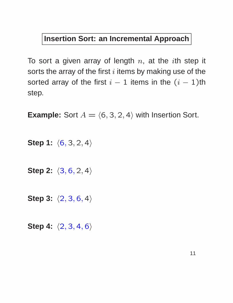
Insertion Sort: an Incremental Approach

To sort a given array of length n, at the ith step itsorts the array of the first i items by making use of thesorted array of the first i − 1 items in the (i − 1)thstep.

Example: Sort A = 〈6,3,2,4〉 with Insertion Sort.

Step 1: 〈6,3,2,4〉

Step 2: 〈3,6,2,4〉

Step 3: 〈2,3,6,4〉

Step 4: 〈2,3,4,6〉

11

Analyzing Algorithms

Predict resource utilization

1. Memory (space complexity)

2. Running time (time complexity)

Remark: Really depends on the model of computa-tion (sequential or parallel). We usually assume se-quential.

12

Analyzing Algorithms – Continued

Running time: the number of primitive operationsused to solve the problem.

Primitive operations: e.g., addition, multiplication,comparisons.

Running time: depends on problem instance, oftenwe find an upper bound: F(input size)

Input size: rigorous definition given later.

1. Sorting: number of items to be sorted

2. Multiplication: number of bits, number of digits.

3. Graphs: number of vertices and edges.

13

Three Cases of Analysis

Best Case: constraints on the input, other than size,resulting in the fastest possible running time.

Worst Case: constraints on the input, other than size,resulting in the slowest possible running time.Example. In the worst case Quicksort runs in Θ(n2)

time on an input of n keys.

Average Case: average running time over every pos-sible type of input (usually involve probabilities of dif-ferent types of input).Example. In the average case Quicksort runs in Θ(n logn)

time on an input of n keys. All n! inputs of n keys areconsidered equally likely.

Remark: All cases are relative to the algorithm underconsideration.

14

Three Analyses of Insertion Sorting

Best Case: A[1] ≤ A[2] ≤ A[3] ≤ · · · ≤ A[n].

The number of comparisons needed is equal to

1 + 1 + 1 + · · · + 1︸ ︷︷ ︸

n−1

= n − 1 = Θ(n).

Worst Case: A[1] ≥ A[2] ≥ A[3] ≥ · · · ≥ A[n].

The number of comparisons needed is equal to

1 + 2 + · · · + (n − 1) =n(n − 1)

2= Θ(n2).

Average Case: Θ(n2) assuming that each of the n!

instances are equally likely.

15

Analytical Time Complexity Analysis

• We would like to compare efficiencies of differentalgorithms for the same problem, instead of differ-ent programs or implementations. This removesdependency on machines and programming skill.

• It becomes meaningless to measure absolute timesince we do not have a particular machine in mind.Instead, we measure the number of steps. Wecall this the time complexity or running time anddenote it by T(n).

• We would like to estimate how T(n) varies withthe input size n.

16

Big-Oh

If A is a much better algorithm than B, then it is notnecessary to calculate TA(n) and TB(n) exactly. Asn increases, since TB(n) will grow much more rapidly,TA(n) will always be less than TB(n) for large enoughn.

Thus, it suffices to measure the growth rate of timecomplexity to get a rough comparison.

f(n) = O(g(n)):

There exists constant c > 0 and n0 such thatf(n) ≤ c · g(n) for n ≥ n0.

17

When estimating the growth rate of T(n) using big-Oh:

• Ignore the low order terms.

• Ignore the constant coefficient of the most signif-icant term.

• The remaining term is the estimate.

18

For example,

• n2/2 − 3n = O(n2)

• 1 + 4n = O(n)

• log10 n = log2 nlog2 10 = O(log2 n) = O(logn)

• sinn = O(1), 10 = O(1), 1010 = O(1).

•∑n

i=1 i2 ≤ n · n2 = O(n3)

•∑n

i=1 i ≤ n · n = O(n2)

• 210n is not O(2n)

• 7n2 + 10n + 3 = O(n2) = O(n3) = O(n4)

19

Big Omega and Big Theta

f(n) = Ω(g(n)) (big-Omega):

There exists constant c > 0 and n0 such thatf(n) ≥ c · g(n) for n ≥ n0.

f(n) = Θ(g(n)) (big-Theta):

f(n) = O(g(n)) and f(n) = Ω(g(n)).

20

Some thoughts on Algorithm Design

• Algorithm Design, as taught in this class, is mainlyabout designing algorithms that have small big-Oh running times.

• “All other things being equal”, O(n logn) algo-rithms will run more quickly than O(n2) ones andO(n) algorithms will beat O(n logn) ones.

• Being able to do good algorithm design lets youidentify the hard parts of your problem and dealwith them effectively.

• Too often, programmers try to solve problems us-ing brute force techniques and end up with slowcomplicated code! A few hours of abstract thoughtdevoted to algorithm design could have speededup the solution substantially and simplified it.

21

Note: After algorithm design one can continue on toAlgorithm tuning which would further concentrate onimproving algorithms by cutting cut down on the con-stants in the big O() bounds. This needs a good un-derstanding of both algorithm design principles andefficient use of data structures. In this course we willnot go further into algorithm tuning. For a good intro-duction, see chapter 9 in Programming Pearls, 2nd edby Jon Bentley.

22