design of machinary
TRANSCRIPT

DESIGN OF MACHINERYAN INTRODUCTION TO THE SYNTHESIS AND
ANALYSIS OF MECHANISMSAND MACHINES
Second Edition

McGraw-Hili Series in Mechanical EngineeringJack P. Holman, Southern Methodist UniversityJohn R. Lloyd, Michigan State UniversityConsulting Editors
Anderson: Modern Compressible Flow: With Historical PerspectiveArora: Introduction to Optimum DesignAnderson: Computational Fluid Dynamics: The Basics with ApplicationsBormanlRagland: Combustion EngineeringBurton: Introduction to Dynamic Systems AnalysisCulp: Principles of Energy ConversionDieter: Engineering Design: A Materials and Processing ApproachDoebelin: Engineering Experimentation: Planning. £-cecution. ReportingDreils: Linear Controls Systems EngineeringEdwards and McKee: Fundamentals of Mechanical Component DesignGebhart: Heat Conduction and Mass DiffusionGibson: Principles of Composite Material MechanicsHamrock: Fundamentals of Fluid Film LubricaIionHeywood: Internal Combustion Engine FundamenralsHinze: TurbulenceHolman: Experimental Methods for EngineersHowell and Buckius: Fundamenrals ofEngiN!ering ThermodynamicsJaluria: Design and Optimi::.ation ofTheTmill SystemsJuvinall: Engineering Considerations of Stress, Strain. and StrengthKays and Crawford: Com'ectiw Heal and Jlass TransferKelly: Fundamentals of Mechanical \'ibrarionsKimbrell: Kinematics Analysis and SynthesisKreider and Rabl: Heating and Cooling of BuildingsMartin: Kinematics and Dynamics ofJlachinesMattingly: Elements of Gas TurbiN! PropulsionModest: Radiati\'e Heat TransferNorton: Design of Machinery: .411 Introduction to the Synthesis and Analysis of
Mechanisms and MachiN!sOosthuizien and CarscaIIeo: Compressible Fluid FlowPhelan: Fundamentals of Mechanical DesignReddy: An Introduction to the Finite Elemen: MethodRosenberg and Kamopp: Introduction to Physical Systems DynamicsSchlichting: Boundary-Layer TheoryShames: Mechanics of FluidsShigley: Kinematic Analysis of MechanismsShigley and Mischke: Mechanical Engineering DesignShigley and Vicker: Theory of Machines and MechanismsStimer: Design with Microprocessors for Mechanical EngineersStoeker and Jones: Refrigeration and Air ConditioningTurns: An Introduction to Combustion: Concepts and ApplicationsUllman: The Mechanical Design ProcessWark: Advanced Thermodynamics for EngineersWhite: Viscous FlowZeid: CAD/CAM Theory and Practice


DESIGN OF MACHINERY: An Introduction to the Synthesis and Analysis ofMechanisms and Machines
Copyright © 1999 by McGraw-Hill Inc. All rights reserved. Previous edition © 1992. Printed inthe United States of America. Except as permitted under the United States Copyright Act of 1976,no part of this publication may be reproduced or distributed in any form or by any means, or storedin a database or retrieval system, without the prior written permission of the publisher.
This book is printed on acid-free paper.
I 2 3 4 5 6 7 8 9 0 QPF/QPF I 0 9 8
ISBN 0-07-048395-7ISBN 0-07-913272-3 (set)ISBN 0-04-847978-9 (CD-ROM)
Vice president and editorial director: Kevin T. KanePublisher: 1bomas CassonSenior sponsoring editor: Debra RiegertDevelopmental editor: Holly StarkMarketing manager: John T. WannemacherProject manager: Christina Thomton- VillagomezProduction supervisor: Michael R. McCormickSupplement Coordinator: Marc MattsonCover Design: Gino CieslikBook design: Wanda SiedleckaPrinter: Quebecor Printing Book Group/Fairfield
Cover photo: Viper cutaway courtesy of the Chrysler Corporation, Auburn Hills, MI.
All text, drawings. and equations in this book were prepared and typeset electronically, by theauthor, on a Mocintosh® computer using Freehan~, MathType®, and Pagemaker® desktoppublishing software. The body text was set in Times Roman, and headings set in Avant Garde.Printer's film color separations were made on a laser typesetter directly from the author's disks.All clip art illustrations are courtesy of Dubl-Click Software Inc., 22521 Styles St., WoodlandHills CA 91367. reprinted from their Industrial Revolution and Old Earth Almanac series withtheir permission (and with the author's thanks).
Library of Congress Cataloging-in-Publication DataNorton, Robert L.
Design of machinery: an introduction to the synthesis and analysis of mechanismsand machines / Robert L. Norton - 2nd ed.
p. cm. --{McGraw-Hill series in mechanical engineering)Includes bibliographical references and index.ISBN 0-07-048395-71. Machinery-Design. 2. Machinery, Kinematics. 3. Machinery,
Dynamics of. I. Title. II. Series.TJ230.N63 1999 91-7510621.8'15-dc20
http://www.mhhe.com

ABOUT THE AUTHOR
Robert L. Norton earned undergraduate degrees in both mechanical engineering and in-dustrial technology at Northeastern University and an MS in engineering design at TuftsUniversity. He is a registered professional engineer in Massachusetts and New Hamp-shire. He has extensive industrial experience in engineering design and manufacturingand many years experience teaching mechanical engineering, engineering design, com-puter science, and related subjects at Northeastern University, Tufts University, andWorcester Polytechnic Institute. At Polaroid Corporation for ten years, he designed cam-eras, related mechanisms, and high-speed automated machinery. He spent three years atJet Spray Cooler Inc., Waltham, Mass., designing food-handling machinery and prod-ucts. For five years he helped develop artificial-heart and noninvasive assisted-circula-tion (counterpulsation) devices at the Tufts New England Medical Center and BostonCity Hospital. Since leaving industry to join academia, he has continued as an indepen-dent consultant on engineering projects ranging from disposable medical products tohigh-speed production machinery. He holds 13 U.S. patents.
Norton has been on the faculty of Worcester Polytechnic Institute since 1981 and iscurrently professor of mechanical engineering and head of the design group in that de-partment. He teaches undergraduate and graduate courses in mechanical engineeringwith emphasis on design, kinematics, and dynamics of machinery. He is the author ofnumerous technical papers and journal articles covering kinematics, dynamics of machin-ery, carn design and manufacturing, computers in education, and engineering educationand of the text Machine Design: An Integrated Approach. He is a Fellow of the Ameri-can Society of Mechanical Engineers and a member of the Society of Automotive Engi-neers. Rumors about the transplantation of a Pentium microprocessor into his brain aredecidedly untrue (though he could use some additional RAM). As for the unobtainium*ring, well, that's another story.
* See Index.

Thisbook isdedicated to the memory of my father,
Harry J. Norton, Sr.
who sparked a young boy's interest in engineering;
to the memory of my mother,
Kathryn W Norton
who made it all possible;
to my wife,
Nancy Norton
who provides unflagging patience and supp~rt;
and to my children,
Robert, Mary, and Thomas,
who make it all worthwhile.

CONTENTSPreface to the Second Edition ................................................................................... XVIIPreface to the First Edition ........................................................................................... XIX
PART I KINEMATICS OF MECHANISMS 1
Chapter 1 Introduction ............................................................................. 3
1.0 Purpose .............................................................................................................. 31.1 Kinematics and Kinetics ................................................................................. 31.2 Mechanisms and Machines ........................................................................... 41.3 A Brief History of Kinematics .......................................................................... 51.4 Applications of Kinematics ............................................................................ 61.5 The Design Process ............ ,............................................................................. 7
Design, Invention, Creativity ....................................................................... 7Identification of Need ................................................................................. 8Background Research .....................................................................··········· 9Goal Statement ........................................................................................... 9Performance Specifications ....................................................................... 9Ideation and Invention ............................................................................. 70Analysis ....................................................................................................... 7 7Selection ..................................................................................................... 72Detailed Design ................................................................................········· 73Prototyping and Testing ............................................................................ 73Production .................................................................................................. 73
1.6 Other Approaches to Design .......................... " ................ " ........ " .............. 14Axiomatic Design ...................................................................................···· 75
1.7 Multiple Solutions ................................................ ,.......................................... 151.8 Human Factors Engineering ............................ " .............. " .................... " .... 151.9 The Engineering Report ................. " ............................................................. 16
1.10 Units ..................................... " ........................................................................... 161.11 What's to Come ........................................................................................... " 181.12 References ........................................................... ,.......................................... 191.13 Bibliography ....................... " ................................ ,.......................................... 20
Chapter 2 Kinematics Fundamentals .................................................. 222.0 Introduction ......................................................... ,........................ " ......... " ..... 222.1 Degrees of Freedom ..................................................................................... 222.2 Types of Motion ................. " ........................................................................... 232.3 Links, Joints, and Kinematic Chains ............................................................ 242.4 Determining Degree of Freedom ............................................. " ................ 28
Degree of Freedom in Planar Mechanisms ... ............ ......... ...... 29Degree of Freedom in Spatial Mechanisms .. ....... .... ......... ..... 32
2.5 Mechanisms and Structures ......................................................................... 322.6 Number Synthesis ....................................................... " ........................ " ........ 332.7 Paradoxes ....................................................................................................... 372.8 Isomers ............................................................................................................. 382.9 Linkage Transformation ................................................................................ 40
2.10 Intermittent Motion ................. " ..................................................................... 422.11 Inversion .......................................................................................................... 44

2.12 The Grashof Condition .................................................................................. 46Classification of the Fourbar Linkage ...................................................... 49
2.13 Linkages of More Than Four Bars ................................................................. 52Geared Fivebar Linkages ......................................................................... 52Sixbar Linkages ........................................................................................... 53Grashof-type Rotatability Criteria for Higher-order Linkages ................ 53
2.14 Springs as Links ............................................................................................... 542.15 Practical Considerations .............................................................................. 55
Pin Joints versusSlidersand Half Joints .................................................... 55Cantilever versusStraddle Mount ............................................................ 57Short Links ................................................................................................ 58Bearing Ratio .............................................................................................. 58Linkages versusCans ...............................................................................59
2.16 Motor and Drives ........................................................................................... 60Electric Motexs ........................................................................................... 60Air and HyaotAc Motexs .......................................................................... 65Air and Hyc:kotAc CyiIders ...................................................................... 65Solenoids ................................................................................................. 66
2.17 References ...................................................................................................... 662.18 Problems .......................................................................................................... 67
Chapter 3 Graphical Linkage Synthesis.............................................. 763.0 Introduction .................................................................................................... 763.1 Synthesis .......................................................................................................... 763.2 Function. Path. and Motion Generation ................................................... 783.3 limiting Conditions ....................................................................................... ,803.4 Dimensional Synthesis ................. ,....... ,........................... ,............................. 82
Two-Posiffon Synthesis................................................................................ 83TPY~n Synthesiswith Specified Moving Pivots ........................... 891hree-Position Synthesiswith Alternate Moving Pivots ........................... 90TPYee-PositionSynthesiswith Specified Fixed Pivots ............................... 93Position Synthesis for More Than Three Positions ..................................... 97
3.5 Quick-Return Mechanisms ............................ ,............................................. ,97Fou'bar Quick-Return ................................................................................ 98SbcbarQuick-Return ................................................................................. 700
3.6 Coupler Curves ............................................ " .................. ,.......................... 1033.7 Cognates .................................... " ........ " ..... ", ....... " ........ " ........ " ....... " ....... 112
Parallel Motion ......................................................................................... 777Geared Rvebar Cognates of the Fourbar ............................................ 779
3.8 Straight-Line Mechanisms .,...... ,........ ", ........................ " ......................... " 120Designing Optimum Straight-Line Fourbar Linkages ............................ 722
3.9 Dwell Mechanisms ............ ,................. ,....... ,.................. ,.......................... " 125Single-Dwell Linkages .............................................................................. 726Double-Dwell Linkages ............................................................................ 728
3.10 References ............................................................. ,........... ,........ ,.............. " 1303.11 Bibliography .......................... ,...... ,....... ,.......................... ", ................. ,........ 1313.12 Problems ............................ " ...... ,.................................................................. 1323.13 Projects ........................................................................ ,................................ 140
Chapter 4 Position Analysis ................................................................. 1444.0 Introduction .............. ,.................. ,....... ,......................... ,............................. 1444.1 Coordinate Systems .......... ,...................... ,................................................. 1464.2 Position and Displacement ....................................................................... 147
Position ...................................................................................................... 747Displacement ........................................................................................... 747

4.3 Translation, Rotation, and Complex Motion .......................................... 149Translation ................................................................................................ 749Rotation .................................................................................................... 749Complex Motion ...................................................................................... 749Theorems .................................................................................................. 750
4.4 Graphical Position Analysis of Linkages .................................................. 1514.5 Algebraic Position Analysis of Linkages .................................................. 152
Vector Loop Representation of Linkages ............................................. 753Complex Numbers as Vectors ............................................................... 754The Vector Loop Equation for a Fourbar Linkage ................................ 756
4.6 The Fourbar Slider-Crank Position Solution ............................................. 1594.7 An Inverted Slider-Crank Position Solution ............................................. 1614.8 Linkages of More Than Four Bars .............................................................. 164
The Geared Fivebar Linkage .................................................................. 764Sixbar Linkages ......................................................................................... 767
4.9 Position of Any Point on a Linkage .......................................................... 1684.10 Transmission Angles .................................................................................... 169
Extreme Values of the TransmissionAngle ............................................ 7694.11 Toggle Positions ........................................................................................... 1714.12 Circuits and Branches in Linkages ........................................................... 1734.13 Newton-Raphson Solution Method ......................................................... 174
One-Dimensional Root-Finding (Newton's Method) ............................ 774Multidimensional Root-Finding (Newton-Raphson Method) ............... 776Newton-Raphson Solution for the Fourbar Linkage ............................. 777Equation Solvers....................................................................................... 778
4.14 References ................................................................................................... 1784.15 Problems ....................................................................................................... 178
Chapter 5 Analytical Linkage Synthesis ........................................... 1885.0 Introduction ................................................................................................. 1885.1 Types of Kinematic Synthesis .................................................................... 1885.2 Precision Points ............................................................................................ 1895.3 Two-Position Motion Generation by Analytical Synthesis .................... 1895.4 Comparison of Analytical and Graphical Two-Position Synthesis ..... 1965.5 Simultaneous Equation Solution ............................................................... 1995.6 Three-Position Motion Generation by Analytical Synthesis ................. 2015.7 Comparison of Analytical and Graphical Three-Position Synthesis ... 2065.8 Synthesis for a Specified Fixed Pivot Location ....................................... 2115.9 Center-Point and Circle-Point Circles ..................................................... 217
5.10 Four- and Five-Position Analytical Synthesis .......................................... 2195.11 Analytical Synthesis of a Path Generator with Prescribed Timing ..... 2205.12 Analytical Synthesis of a Fourbar Function Generator ........................ 2205.13 Other Linkage Synthesis Methods ............................................................ 224
Precision Point Methods .......................................................................... 226CouplerCuNe Equation Methods ......................................................... 227Optimization Methods ............................................................................. 227
5.14 References ................................................................................................... 2305.15 Problems .............................................................. ,........................................ 232
Chapter 6 Velocity Analysis ................................................................ 2416.0 Introduction ........................................................ ,........................................ 2416.1 Definition of Velocity ......................................... ,........................................ 2416.2 Graphical Velocity Analysis ...................................................................... 244

6.3 Instant Centers of Velocity ........................................................................ 2496.4 Velocity Analysis with Instant Centers ..................................................... 256
Angular Velocity Raffo ............................................................................ 257Mechanical Advantage ......................................................................... 259Using Instant Centers in Unkage Design ................................................ 267
6.5 Centrodes .................................................................................................... 263A 'UnkJess-Unkage ................................................................................. 266Cusps ........................................................................................................ 267
6.6 Velocity of Slip ............................................................................................. 2676.7 Analytical Solutions for Velocity Analysis ................................................ 271
The FotIbar Pin-Jointed Unkage ............................................................ 277The FotIbar Slider-Crank ......................................................................... 274The FotIbar Inverted Slider-Crank ......................................................... 276
6.8 Velocity Analysis of the Geared Fivebar Linkage ................................. 2786.9 Velocity of Any Point on a Linkage ......................................................... 279
6.10 References ................................................................................................... 2806.11 Problems ....................................................................................................... 281
Chapter 7 Acceleration Analysis ....................................................... 3007.0 Introduction ................................................................................................. 3007.1 Definition of Acceleration ......................................................................... 3007.2 Graphical Acceleration Analysis ............................................................. 3037.3 Analytical Solutions for Acceleration Analysis ....................................... 308
The Fourbar Pin-Jointed Linkage ............................................................ 308The Fourbar Slider-Crank ......................................................................... 377CorioIis Acceleration ............................................................................'" 3 73The Fourbar Inverted Slider-Crank ......................................................... 375
7.4 Acceleration Analysis of the Geared Fivebar Linkage ........................ 3197.5 Acceleration of any Point on a Linkage ................................................ 3207.6 Human Tolerance of Acceleration .......................................................... 3227.7 Jerk ................................................................................................................ 3247.8 Linkages of N Bars ....................................................................................... 3277.9 References ................................................................................................... 327
7.10 Problems ....................................................................................................... 327
Chapter 8 Cam Design ........................................................................ 3458.0 Introduction ................................................................................................. 3458.1 Cam Terminology ....................................................................................... 346
Type of Follower Motion .......................................................................... 347Type of Joint Closure ............................................................................... 348Type of Follower ....................................................................................... 348Type of Cam ............................................................................................ 348Type of Motion Constraints ..................................................................... 357Type of Motion Program ......................................................................... 357
8.2 S V A J Diagrams ........................................................................................ 3528.3 Double-Dwell Cam Design-Choosing S V A J Functions ................... 353
TheFundamental LawofCamDesign .................................................. 356Simple Harmonic Motion (SHM) ............................................................. 357Cycloidal Displacement ......................................................................... 359Combined Functions ............................................................................... 362
8.4 Single-Dwell Cam Design-Choosing S V A J Functions ...................... 3748.5 Polynomial Functions ................................................................................. 378
Double-Dwell Applications of Polynomials ........................................... 378Single-Dwell Applications of Polynomials .............................................. 382

8.6 Critical Path Motion (CPM) ...................................................................... 385Polynomials Used for Critical Path Motion ............................................ 386Half-Period Harmonic Family Functions ................................................. 393
8.7 Sizing the Com-Pressure Angle and Radius of Curvature ................. 396PressureAngle-Roller Followers ............................................................ 397Choosing a Prime Circle Radius ............................................................. 400Overturning Moment-Flat-Faced Follower ......................................... 402Radius of Curvature-Roller Follower .................................................... 403Radius of Curvature-Flat-Faced Follower ........................................... 407
8.8 Com Manufacturing Considerations ...................................................... 412Geometric Generation ........................................................................... 413Manual or NC Machining to Cam Coordinates (Plunge-Cutting) ..... 413Continuous Numerical Control with Linear Interpolation .................... 414Continuous Numerical Control with Circular Interpolation ................. 416Analog Duplication ................................................................................. 416Actual Cam Performance Compared to Theoretical Performance. 418
8.9 Practical Design Considerations .............................................................. 421Translating or Oscillating Follower? ........................................................ 421Force- or Form-Closed? ,......................................................................... 422Radial or Axial Cam? .............................................................................. 422Roller or Flat-Faced Follower? ................................................................ 423ToDwell or Not to Dwell? ........................................................................ 423ToGrind or Not to Grind? ........................................................................ 424ToLubricate or Not to Lubricate? .......................................................... 424
8.10 References ................................................................................................... 4248.11 Problems ................................................................................................... ,... 4258.12 Projects ......................................................................................................... 429
Chapter 9 Gear Trains.......................................................................... 4329.0 Introduction ................................................................................................. 4329.1 Rolling Cylinders .......................................................................................... 4339.2 The Fundamental Law of Gearing ........................................................... 434
The Involute Tooth Form .......................................................................... 435PressureAngle .......................................................................................... 437Changing Center Distance .................................................................... 438Backlash ................................................................................................... 438
9.3 Gear Tooth Nomenclature ........................................................................ 4409.4 Interference and Undercutting ................................................................ 442
Unequal-Addendum Tooth Forms ......................................................... 4449.5 Contact Ratio .............................................................................................. 4449.6 Gear Types ................................................................................................... 447
Spur, Helical, and Herringbone Gears ................................................... 447Worms and Worm Gears ........................................................................ 448Rack and Pinion ....................................................................................... 448Bevel and Hypoid Gears ......................................................................... 449Noncircular Gears ................................................................................... 450Belt and Chain Drives .............................................................................. 450
9.7 Simple Gear Trains ...................................................................................... 4529.8 Compound Gear Trains .,........................................................................... 453
Design of Compound Trains................................................................... 454Design of Reverted Compound Trains.................................................. 456An Algorithm for the Design of Compound Gear Trains ..................... 458
9.9 Epicyclic or Planetary Gear Trains ........................................................... 462The Tabular Method ................................................................................ 464TheFormula Method ...,........................................................................... 469
9.10 Efficiency of Gear Trains ............................................................................ 470


Chapter 15 Com Dynamics ................................................................ 68515.0 Introduction .................................................................................................68515.1 Dynamic Force Analysis of the Force-Closed Cam Follower .............686
Undamped Response, ............................................................................ 686Damped Response ................................................................................. 689
15.2 Resonance ...................................................................................................69615.3 Kinetostatic Force Analysis of the Force-Closed Cam-Follower ........ 69815.4 Kinetostatic Force Analysis of the Form-Closed Cam-Follower. ......... 70215.5 Camshaft Torque ........................................................................................70615.6 Measuring Dynamic Forces and Accelerations ....................................70915.7 Practical Considerations ...........................................................................71315.8 References ...................................................................................................71315.9 Bibliography .................................................................................................713
15.10 Problems .......................................................................................................714
Chapter 16 Engineering Design .......................................................... 71716.0 Introduction .................................................................................................71716.1 A Design Case Study ..................................................................................71816.2 Closure ..........................................................................................................72316.3 References ...................................................................................................723
Appendix A Computer Programs ....................................................... 725AO Introduction .................................................................................................725A1 General Information ..................................................................................727A2 General Program Operation ....................................................................727A3 Program FOURBAR.........................................................................................735A4 Program FIVEBAR...........................................................................................743A5 Program SIXBAR............................................................................................745A6 Program SLIDER.............................................................................................749A7 Program DVNACAM......................................................................................751A8 Program ENGINE...........................................................................................757A9 Program MATRIX............,...............................................................................764
Appendix B Material Properties.......................................................... 765
Appendix C Geometric Properties .................................................... 769
Appendix D Spring Data ...................................................................... 771
Appendix E Atlas of Geared Fivebar Linkage Coupler Curves ..... 775
Appendix F Answers to Selected Problems ...................................... 781
Index .........................................,................................................................ 795
CD - ROM Index .......................................................................................... 809

PREFACEto the Second Edition
Why is it we never have time to doit right the first time, but alwaysseem to have time to do it over?ANONYMOUS
The second edition has been revised based on feedback from a large number of users of thebook. In general, the material in many chapters has been updated to reflect the latest researchfindings in the literature. Over 250 problem sets have been added, more than doubling thetotal number of problems. Some design projects have been added also. All the illustrationshave been redrawn, enhanced, and improved.
Coverage of the design process in Chapter 1 has been expanded. The discussions of theGrashof condition and rotatability criteria in Chapter 2 have been strengthened and that ofelectric motors expanded. A section on the optimum design of approximate straight line link-ages has been added to Chapter 3. A discussion of circuits and branches in linkages and asection on the Newton-Raphson method of solution have been added to Chapter 4. A discus-sion of other methods for analytical and computational solutions to the position synthesisproblem has been added to Chapter 5. This reflects the latest publications on this subject andis accompanied by an extensive bibliography.
The chapters formerly devoted to explanations of the accompanying software (old Chap-ters 8 and 16) have been eliminated. Instead, a new Appendix A has been added to describethe programs FOURBAR,FIVEBAR,SrXBAR,SLIDER,DYNACAM,ENGINE,and MATRIXthat areon the attached CD-ROM. These programs have been completely rewritten as Windows ap-plications and are much improved. A student version of the simulation program WorkingModel by Knowledge Revolution, compatible with both Macintosh and Windows computers,is also included on CD-ROM along with 20 models of mechanisms from the book done inthat package. A user's manual for Working Model is also on the CD-ROM.
Chapter 8 on cam design (formerly 9) has been shortened without reducing the scope of itscoverage. Chapter 9 on gear trains (formerly 10)has been significantly expanded and enhanced,especially in respect to the design of compound and epicyclic trains and their efficiency. Chapter10on dynamics fundamentals has been augmented with material formerly in Chapter 17 to give amore coherent treatment of dynamic modeling. Chapter 12 on balancing (formerly 13)has beenexpanded to include discussion of moment balancing of linkages.
The author would like to express his appreciation to all the users and reviewers who havemade suggestions for improvement and pointed out errors, especially those who responded to thesurvey about the first edition. There are too many to list here, so rather than risk offense by omit-ting anyone, let me simply extend my sincerest thanks to you all for your efforts.
'.1{p6ertL. 'J,{prton:Mattapoisettl :Mass.
5tugustl 1997

PREFACEto the First Edition
When I hear, I forgetWhen I see, I rememberWhen I do, I understandANCIENT CHINESE PROVERB
This text is intended for the kinematics and dynamics of machinery topics which are of-ten given as a single course, or two-course sequence, in the junior year of most mechan-ical engineering programs. The usual prerequisites are first courses in statics, dynamicsand calculus. Usually, the first semester, or portion, is devoted to kinematics, and the sec-ond to dynamics of machinery. These courses are ideal vehicles for introducing the me-chanical engineering student to the process of design, since mechanisms tend to be intu-itive for the typical mechanical engineering student to visualize and create. While thistext attempts to be thorough and complete on the topics of analysis, it also emphasizesthe synthesis and design aspects of the subject to a greater degree than most texts in printon these subjects. Also, it emphasizes the use of computer-aided engineering as an ap-proach to the design and analysis of this class of problems by providing software that canenhance student understanding. While the mathematical level of this text is aimed at sec-ond- or third-year university students, it is presented de novo and should be understand-able to the technical school student as well.
Part I of this text is suitable for a one-semester or one-term course in kinematics.Part II is suitable for a one-semester or one-term course in dynamics of machinery. Alter-natively, both topic areas can be covered in one semester with less emphasis on some ofthe topics covered in the text.
The writing and style of presentation in the text is designed to be clear, informal, andeasy to read. Many example problems and solution techniques are presented and spelledout in detail, both verbally and graphically. All the illustrations are done with computer-drawing or drafting programs. Some scanned photographic images are also included.The entire text, including equations and artwork, is printed directly from computer diskby laser typesetting for maximum clarity and quality. Many suggested readings are pro-vided in the bibliography. Short problems, and where appropriate, many longer, unstruc-tured design project assignments are provided at the ends of chapters. These projectsprovide an opportunity for the students to do and understand.
The author's approach to these courses and this text is based on over 35 years'experience in mechanical engineering design, both in industry and as a consultant.He has taught these subjects since 1967, both in evening school to practicing engi-neers and in day school to younger students. His approach to the course has evolved

a great deal in that time, from a traditional approach, emphasizing graphical analysis ofmany structured problems, through emphasis on algebraic methods as computers be-came available, through requiring students to write their own computer programs, tothe current state described above.
The one constant throughout has been the attempt to convey the art of the design pro-cess to the students in order to prepare them to cope with real engineering problems inpractice. Thus, the author has always promoted design within these courses. Only re-cently, however, has technology provided a means to more effectively accomplish thisgoal, in the form of the graphics microcomputer. This text attempts to be an improve-ment over those currently available by providing up-to-date methods and techniques foranalysis and synthesis which take full advantage of the graphics microcomputer, and byemphasizing design as well as analysis. The text also provides a more complete, mod-em, and thorough treatment of cam design than existing texts in print on the subject.
The author has written several interactive, student-friendly computer programs forthe design and analysis of mechanisms and machines. These programs are designed toenhance the student's understanding of the basic concepts in these courses while simul-taneously allowing more comprehensive and realistic problem and project assignmentsto be done in the limited time available, than could ever be done with manual solutiontechniques, whether graphical or algebraic. Unstructured, realistic design problems whichhave many valid solutions are assigned. Synthesis and analysis are equally emphasized.The analysis methods presented are up to date, using vector equations and matrix tech-niques wherever applicable. Manual graphical analysis methods are de-emphasized. Thegraphics output from the computer programs allows the student to see the results of vari-ation of parameters rapidly and accurately and reinforces learning.
These computer programs are distributed, on CD-ROM, with this book which alsocontains instructions for their use on any IBM compatible, Windows 3.1 or Windows 95/NT capable computer. The earlier DOS versions of these programs are also included forthose without access to Windows. Programs SLIDER,FOURBAR,FIVEBARand SIXBARan-alyze the kinematics of those types of linkages. Program FOURBARalso does a completedynamic analysis of the fourbar linkage in addition to its kinematics. Program DYNACAMallows the design and dynamic analysis of cam-follower systems. Program ENGINEan-alyzes the slider-crank linkage as used in the internal combustion engine and provides acomplete dynamic analysis of single and multicylinder engine configurations, allowingthe mechanical dynamic design of engines to be done. Program MATRIXis a general pur-pose linear equation system solver. All these programs, except MATRIX,provide dynam-ic, graphical animation of the designed devices. The reader is strongly urged to make useof these programs in order to investigate the results of variation of parameters in these ki-nematic devices. The programs are designed to enhance and augment the text rather thanbe a substitute for it. The converse is also true. Many solutions to the book's examplesand to the problem sets are provided on the CD-ROM as files to be read into these pro-grams. Many of these solutions can be animated on the computer screen for a better dem-onstration of the concept than is possible on the printed page. The instructor and studentsare both encouraged to take advantage of the computer programs provided. Instructionsfor their use are in Appendix A.
The author's intention is that synthesis topics be introduced first to allow thestudents to work on some simple design tasks early in the term while still mastering

the analysis topics. Though this is not the "traditional" approach to the teaching ofthis material, the author believes that it is a superior method to that of initial concen-tration on detailed analysis of mechanisms for which the student has no concept of or-igin or purpose. Chapters 1 and 2 are introductory. Those instructors wishing toteach analysis before synthesis can leave Chapters 3 and 5 on linkage synthesis forlater consumption. Chapters 4, 6, and 7 on position, velocity, and acceleration anal-ysis are sequential and build upon each other. In fact, some of the problem sets are com-mon among these three chapters so that students can use their position solutions to findvelocities and then later use both to find the accelerations in the same linkages.Chapter 8 on cams is more extensive and complete than that of other kinematics textsand takes a design approach. Chapter 9 on gear trains is introductory. The dynamic forcetreatment in Part II uses matrix methods for the solution of the system simultaneousequations. Graphical force analysis is not emphasized. Chapter 10 presents an intro-duction to dynamic systems modelling. Chapter 11 deals with force analysis oflinkag-es. Balancing of rotating machinery and linkages is covered in Chapter 12. Chapters 13and 14 use the internal combustion engine as an example to pull together many dynamicconcepts in a design context. Chapter 15 presents an introduction to dynamic systemsmodelling and uses the cam-follower system as the example. Chapters 3, 8, 11, 13,and 14 provide open ended project problems as well as structured problem sets. Theassignment and execution of unstructured project problems can greatly enhance thestudent's understanding of the concepts as described by the proverb in the epigraphto this preface.
ACKNOWLEDGMENTS The sources of photographs and other nonoriginal artused in the text are acknowledged in the captions and opposite the title page, but theauthor would also like to express his thanks for the cooperation of all those individ-uals and companies who generously made these items available. The author wouldalso like to thank those who have reviewed various sections of the first edition of thetext and who made many useful suggestions for improvement. Mr. John Titus of theUniversity of Minnesota reviewed Chapter 5 on analytical synthesis and Mr. DennisKlipp of Klipp Engineering, Waterville, Maine, reviewed Chapter 8 on cam design.Professor William J. Crochetiere and Mr. Homer Eckhardt of Tufts University, Med-ford, Mass., reviewed Chapter 15. Mr. Eckhardt and Professor Crochetiere of Tufts,and Professor Charles Warren of the University of Alabama taught from and re-viewed Part I. Professor Holly K. Ault of Worcester Polytechnic Institute thorough-ly reviewed the entire text while teaching from the pre-publication, class-test ver-sions of the complete book. Professor Michael Keefe of the University of Delawareprovided many helpful comments. Sincere thanks also go to the large number of un-dergraduate students and graduate teaching assistants who caught many typos and errorsin the text and in the programs while using the pre-publication versions. Since the book'sfirst printing, Profs. D. Cronin, K. Gupta, P. Jensen, and Mr. R. Jantz have written to pointout errors or make suggestions which I have incorporated and for which I thank them.The author takes full responsibility for any errors that may remain and invites from allreaders their criticisms, suggestions for improvement, and identification of errors in thetext or programs, so that both can be improved in future versions.
'R.P6ertL. :lI{prton:Mattapoisett/ :Mass.
5lugust/ 1991

Take to Kinematics. It will repay you. It ismore fecund than geometry;it adds a fourth dimension to space.
CHEBYSCHEV TO SYLVESTER, 1873

1.0 PURPOSE
In this text we will explore the topics of kinematics and dynamics of machinery in re-spect to the synthesis of mechanisms in order to accomplish desired motions or tasks,and also the analysis of mechanisms in order to determine their rigid-body dynamicbehavior. These topics are fundamental to the broader subject of machine design. Onthe premise that we cannot analyze anything until it has been synthesized into existence,we will first explore the topic of synthesis of mechanisms. Then we will investigatetechniques of analysis of mechanisms. All this will be directed toward developing yourability to design viable mechanism solutions to real, unstructured engineering problemsby using a design process. We will begin with careful definitions of the terms used inthese topics.
1.1 KINEMATICS AND KINETICS
KINEMATICS The study of motion without regard to forces.
KINETIcs The study of forces on systems in motion.
These two concepts are really not physically separable. We arbitrarily separate them forinstructional reasons in engineering education. It is also valid in engineering designpractice to first consider the desired kinematic motions and their consequences, and thensubsequently investigate the kinetic forces associated with those motions. The studentshould realize that the division between kinematics and kinetics is quite arbitrary andis done largely for convenience. One cannot design most dynamic mechanical systemswithout taking both topics into thorough consideration. It is quite logical to considerthem in the order listed since, from Newton's second law, F = ma, one typically needs to
3

know the accelerations (a) in order to compute the dynamic forces (F) due to the mo-tion of the system's mass (m). There are also many situations in which the applied forc-es are known and the resultant accelerations are to be found.
One principal aim of kinematics is to create (design) the desired motions of the sub-ject mechanical parts and then mathematically compute the positions, velocities, and ac-celerations which those motions will create on the parts. Since, for most earthboundmechanical systems, the mass remains essentially constant with time, defining the accel-erations as a function of time then also defines the dynamic forces as a function of time.Stresses, in turn, will be a function of both applied and inertial (ma) forces. Since engi-neering design is charged with creating systems which will not fail during their expectedservice life, the goal is to keep stresses within acceptable limits for the materials chosenand the environmental conditions encountered. This obviously requires that all systemforces be defined and kept within desired limits. In machinery which moves (the onlyinteresting kind), the largest forces encountered are often those due to the dynamics ofthe machine itself. These dynamic forces are proportional to acceleration, which bringsus back to kinematics, the foundation of mechanical design. Very basic and early deci-sions in the design process involving kinematic principles can be crucial to the successof any mechanical design. A design which has poor kinematics will prove troublesomeand perform badly.
1.2 MECHANISMS AND MACHINES
A mechanism is a device which transforms motion to some desirable pattern and typi-cally develops very low forces and transmits little power. A machine typically containsmechanisms which are designed to provide significant forces and transmit significantpowerJI] Some examples of common mechanisms are a pencil sharpener, a camera shut-ter, an analog clock, a folding chair, an adjustable desk lamp, and an umbrella. Someexamples of machines which possess motions similar to the mechanisms listed above area food blender, a bank vault door, an automobile transmission, a bulldozer, a robot, andan amusement park ride. There is no clear-cut dividing line between mechanisms andmachines. They differ in degree rather than in kind. If the forces or energy levels withinthe device are significant, it is considered a machine; if not, it is considered a mechanism.A useful working definition of a mechanism is A system of elements arranged to trans-mit motion in a predetermined fashion. This can be converted to a definition of a ma-chine by adding the words and energy after motion.
Mechanisms, if lightly loaded and run at slow speeds, can sometimes be treatedstrictly as kinematic devices; that is, they can be analyzed kinematically without regardto forces. Machines (and mechanisms running at higher speeds), on the other hand, mustfirst be treated as mechanisms, a kinematic analysis of their velocities and accelerationsmust be done, and then they must be subsequently analyzed as dynamic systems in whichtheir static and dynamic forces due to those accelerations are analyzed using the princi-ples of kinetics. Part I of this text deals with Kinematics of Mechanisms, and Part IIwith Dynamics of Machinery. The techniques of mechanism synthesis presented in PartI are applicable to the design of both mechanisms and machines, since in each case somecollection of moveable members must be created to provide and control the desiredmotions and geometry.

1.3 A BRIEFHISTORY OF KINEMATICS
Machines and mechanisms have been devised by people since the dawn of history. Theancient Egyptians devised primitive machines to accomplish the building of the pyra-mids and other monuments. Though the wheel and pulley (on an axle) were not knownto the Old Kingdom Egyptians, they made use of the lever, the inclined plane (or wedge),and probably the log roller. The origin of the wheel and axle is not definitively known.Its first appearance seems to have been in Mesopotamia about 3000 to 4000 B.C.
A great deal of design effort was spent from early times on the problem of timekeep-ing as more sophisticated clockworks were devised. Much early machine design wasdirected toward military applications (catapults, wall scaling apparatus, etc.). The termcivil engineering was later coined to differentiate civilian from military applications oftechnology. Mechanical engineering had its beginnings in machine design as the in-ventions of the industrial revolution required more complicated and sophisticated solu-tions to motion control problems. James Watt (1736-1819) probably deserves the titleof first kinematician for his synthesis of a straight-line linkage (see Figure 3-29a on p.121) to guide the very long stroke pistons in the then new steam engines. Since the plan-er was yet to be invented (in 1817), no means then existed to machine a long, straightguide to serve as a crosshead in the steam engine. Watt was certainly the first on recordto recognize the value of the motions of the coupler link in the fourbar linkage. OliverEvans (1755-1819) an early American inventor, also designed a straight-line linkage fora steam engine. Euler (1707-1783) was a contemporary of Watt, though they apparent-ly never met. Euler presented an analytical treatment of mechanisms in his Mechanicasive Motus Scienta Analytice Exposita (1736-1742), which included the concept that pla-nar motion is composed of two independent components, namely, translation of a pointand rotation of the body about that point. Euler also suggested the separation of the prob-lem of dynamic analysis into the "geometrical" and the "mechanical" in order to simpli-fy the determination of the system's dynamics. Two of his contemporaries, d' Alembertand Kant, also proposed similar ideas. This is the origin of our division of the topic intokinematics and kinetics as described above.
In the early 1800s, L'Ecole Polytechnic in Paris, France, was the repository of engi-neering expertise. Lagrange and Fourier were among its faculty. One of its founderswas Gaspard Monge (1746-1818), inventor of descriptive geometry (which incidental-ly was kept as a military secret by the French government for 30 years because of itsvalue in planning fortifications). Monge created a course in elements of machines andset about the task of classifying all mechanisms and machines known to mankind! Hiscolleague, Hachette, completed the work in 1806 and published it as what was probablythe first mechanism text in 1811. Andre Marie Ampere (1775-1836), also a professorat L'Ecole Polytechnic, set about the formidable task of classifying "all human knowl-edge." In his Essai sur la Philosophie des Sciences, he was the first to use the term "ein-ematique," from the Greek word for motion,* to describe the study of motion withoutregard to forces, and suggested that "this science ought to include all that can be said withrespect to motion in its different kinds, independently of the forces by which it is pro-duced." His term was later anglicized to kinematics and germanized to kinematik.
Robert Willis (1800-1875) wrote the text Principles of Mechanism in 1841 while aprofessor of natural philosophy at the University of Cambridge, England. He attemptedto systematize the task of mechanism synthesis. He counted five ways of obtaining rel-
* Ampere is quoted aswriting "(The science ofmechanisms) musttherefore not define amachine, as has usuallybeen done, as an instru-ment by the help of whichthe direction and intensityof a given force can bealtered, but as aninstrument by the help ofwhich the direction andvelocity of a given motioncan be altered. To thisscience ... Ihave given thename Kinematics fromKtVIl<x-motion." inMaunder, L. (1979)."Theory and Practice."Proc. 5th World Congo onTheory of Mechanisms andMachines, Montreal, p. I.

ative motion between input and output links: rolling contact, sliding contact, linkages,wrapping connectors (belts, chains), and tackle (rope or chain hoists). Franz Reuleaux(1829-1905), published Theoretische Kinematik in 1875. Many of his ideas are still cur-rent and useful. Alexander Kennedy (1847-1928) translated Reuleaux into English in1876. This text became the foundation of modem kinematics and is still in print! (Seebibliography at end of chapter.) He provided us with the concept of a kinematic pair(joint), whose shape and interaction define the type of motion transmitted between ele-ments in the mechanism. Reuleaux defined six basic mechanical components: the link,the wheel, the cam, the screw, the ratchet, and the belt. He also defined "higher" and"lower" pairs, higher having line or point contact (as in a roller or ball bearing) and low-er having surface contact (as in pin joints). Reuleaux is generally considered the fatherof modem kinematics and is responsible for the symbolic notation of skeletal, genericlinkages used in all modem kinematics texts.
In this century, prior to World War II, most theoretical work in kinematics was donein Europe, especially in Germany. Few research results were available in English. Inthe United States, kinematics was largely ignored until the 1940s, when A. E. R. De-Jonge wrote "What Is Wrong with 'Kinematics' and 'Mechanisms'?,"[2] which calledupon the U.S. mechanical engineering education establishment to pay attention to the Eu-ropean accomplishments in this field. Since then, much new work has been done, espe-cially in kinematic synthesis, by American and European engineers and researchers suchas J. Denavit, A. Erdman, F. Freudenstein, A. S. Hall, R. Hartenberg, R. Kaufman,B. Roth, G. Sandor, andA. Soni, (all of the U.S.) and K. Hain (of Germany). Since thefall of the "iron curtain" much original work done by Soviet Russian kinematicians hasbecome available in the United States, such as that by Artobolevsky.[3] Many U.S. re-searchers have applied the computer to solve previously intractable problems, both ofanalysis and synthesis, making practical use of many of the theories of their predeces-sors.[4] This text will make much use of the availability of computers to allow more ef-ficient analysis and synthesis of solutions to machine design problems. Several comput-er programs are included with this book for your use.
1.4 APPLICATIONS OF KINEMATICS
One of the first tasks in solving any machine design problem is to determine the kine-matic configuration(s) needed to provide the desired motions. Force and stress analysestypically cannot be done until the kinematic issues have been resolved. This text address-es the design of kinematic devices such as linkages, cams, and gears. Each of these termswill be fully defined in succeeding chapters, but it may be useful to show some exam-ples of kinematic applications in this introductory chapter. You probably have used manyof these systems without giving any thought to their kinematics.
Virtually any machine or device that moves contains one or more kinematic ele-ments such as linkages, cams, gears, belts, chains. Your bicycle is a simple example of akinematic system that contains a chain drive to provide torque multiplication and sim-ple cable-operated linkages for braking. An automobile contains many more examplesof kinematic devices. Its steering system, wheel suspensions, and piston-engine all con-tain linkages; the engine's valves are opened by cams; and the transmission is full ofgears. Even the windshield wipers are linkage-driven. Figure l-la shows a spatial link-age used to control the rear wheel movement of a modem automobile over bumps.

Construction equipment such as tractors, cranes, and backhoes all use linkages ex-tensively in their design. Figure 1-1b shows a small backhoe that is a linkage driven byhydraulic cylinders. Another application using linkages is thatof exercise equipment asshown in Figure I-Ie. The examples in Figure 1-1 are all of consumer goods which youmay encounter in your daily travels. Many other kinematic examples occur in the realmof producer goods-machines used to make the many consumer products that we use.You are less likely to encounter these outside of a factory environment. Once you be-come familiar with the terms and principles of kinematics, you will no longer be able tolook at any machine or product without seeing its kinematic aspects.
1.5 THE DESIGN PROCESS
Design, Invention, CreativityThese are all familiar terms but may mean different things to different people. Theseterms can encompass a wide range of activities from styling the newest look in clothing,to creating impressive architecture, to engineering a machine for the manufacture of fa-cial tissues. Engineering design, which we are concerned with here, embodies all threeof these activities as well as many others. The word design is derived from the Latindesignare, which means "to designate, or mark out." Webster's gives several defini-tions, the most applicable being "to outline, plot, or plan, as action or work ... to con-ceive, invent- contrive." Engineering design has been defined as "... the process ofap-plying the various techniques and scientific principles for the purpose of defining a de-vice, a process or a system in sufficient detail to permit its realization ... Design maybe simple or enormously complex, easy or difficult, mathematical or nonmathematical;it may involve a trivial problem or one of great importance." Design is a universal con-stituent of engineering practice. But the complexity of engineering subjects usually re-

DESIGN OF MACHINERY CHAPTER 1
quires that the student be served with a collection of structured, set-piece problemsdesigned to elucidate a particular concept or concepts related to the particular topic.These textbook problems typically take the form of "given A, B, C, and D, find E." Un-fortunately, real-life engineering problems are almost never so structured. Real designproblems more often take the form of "What we need is a framus to stuff this widget intothat hole within the time allocated to the transfer of this other gizmo." The new engi-neering graduate will search in vain among his or her textbooks for much guidance tosolve such a problem. This unstructured problem statement usually leads to what iscommonly called "blank paper syndrome." Engineers often find themselves staring ata blank sheet of paper pondering how to begin solving such an ill-defined problem.
Much of engineering education deals with topics of analysis, which means to de-compose, to take apart, to resolve into its constituent parts. This is quite necessary. Theengineer must know how to analyze systems of various types, mechanical, electrical,thermal, or fluid. Analysis requires a thorough understanding of both the appropriatemathematical techniques and the fundamental physics of the system's function. But,before any system can be analyzed, it must exist, and a blank sheet of paper provides lit-tle substance for analysis. Thus the first step in any engineering design exercise is thatof synthesis, which means putting together.
The design engineer, in practice, regardless of discipline, continuously faces thechallenge of structuring the unstructured problem. Inevitably, the problem as posed tothe engineer is ill-defined and incomplete. Before any attempt can be made to analyzethe situation he or she must first carefully define the problem, using an engineering ap-proach, to ensure that any proposed solution will solve the right problem. Many exam-ples exist of excellent engineering solutions which were ultimately rejected because theysolved the wrong problem, i.e., a different one than the client really had.
Much research has been devoted to the definition of various "design processes" in-tended to provide means to structure the unstructured problem and lead to a viable solu-tion. Some of these processes present dozens of steps, others only a few. The one pre-sented in Table 1-1 contains 10 steps and has, in the author's experience, proven success-ful in over 30 years of practice in engineering design.
ITERATION Before discussing each of these steps in detail it is necessary to pointout that this is not a process in which one proceeds from step one through ten in a linearfashion. Rather it is, by its nature, an iterative process in which progress is made halt-ingly, two steps forward and one step back. It is inherently circular. To iterate means torepeat, to return to a previous state. If, for example, your apparently great idea, uponanalysis, turns out to violate the second law of thermodynamics, you can return to theideation step and get a better idea! Or, if necessary, you can return to an earlier step inthe process, perhaps the background research, and learn more about the problem. Withthe understanding that the actual execution of the process involves iteration, for simplic-ity, we will now discuss each step in the order listed in Table 1-1.
Identification of Need
This first step is often done for you by someone, boss or client, saying "What we need is... " Typically this statement will be brief and lacking in detail. It will fall far short ofproviding you with a structured problem statement. For example, the problem statementmight be "We need a better lawn mower."

Background Research
This is the most important phase in the process, and is unfortunately often the most ne-glected. The term research, used in this context, should not conjure up visions of white-coated scientists mixing concoctions in test tubes. Rather this is research of a moremundane sort, gathering background information on the relevant physics, chemistry, orother aspects of the problem. Also it is desirable to find out if this, or a similar problem,has been solved before. There is no point in reinventing the wheel. If you are luckyenough to find a ready-made solution on the market, it will no doubt be more economi-cal to purchase it than to build your own. Most likely this will not be the case, but youmay learn a great deal about the problem to be solved by investigating the existing "art"associated with similar technologies and products. The patent literature and technicalpublications in the subject area are obvious sources of information and are accessible viathe worldwide web. Clearly, if you find that the solution exists and is covered by a patentstill in force, you have only a few ethical choices: buy the patentee's existing solution,design something which does not conflict with the patent, or drop the project. It is veryimportant that sufficient energy and time be expended on this research and preparationphase of the process in order to avoid the embarrassment of concocting a great solutionto the wrong problem. Most inexperienced (and some experienced) engineers give toolittle attention to this phase and jump too quickly into the ideation and invention stage ofthe process. This must be avoided! You must discipline yourself to not try to solve theproblem before thoroughly preparing yourself to do so.
Goal Statement
Once the background of the problem area as originally stated is fully understood, youwill be ready to recast that problem into a more coherent goal statement. This new prob-lem statement should have three characteristics. It should be concise, be general, and beuncolored by any terms which predict a solution. It should be couched in terms of func-tional visualization, meaning to visualize its function, rather than any particular embod-iment. For example, if the original statement of need was "Design a Better Lawn Mow-er," after research into the myriad of ways to cut grass that have been devised over theages, the wise designer might restate the goal as "Design a Means to Shorten Grass."The original problem statement has a built-in trap in the form of the colored words "lawnmower." For most people, this phrase will conjure up a vision of something with whir-ring blades and a noisy engine. For the ideation phase to be most successful, it is neces-sary to avoid such images and to state the problem generally, clearly, and concisely. Asan exercise, list 10 ways to shorten grass. Most of them would not occur to you had youbeen asked for 10 better lawn mower designs. You should use functional visualizationto avoid unnecessarily limiting your creativity!
Performance Specifications'
When the background is understood, and the goal clearly stated, you are ready to formu-late a set of performance specifications. These should not be design specifications. Thedifference is that performance specifications define what the system must do, while de-sign specifications define how it must do it. At this stage of the design process it is un-wise to attempt to specify how the goal is to be accomplished. That is left for the ide-ation phase. The purpose of the performance specifications is to carefully define and

constrain the problem so that it both can be solved and can be shown to have been solvedafter the fact. A sample set of performance specifications for our "grass shortener" isshown in Table 1-2.
Note that these specifications constrain the design without overly restricting theengineer's design freedom. It would be inappropriate to require a gasoline engine forspecification 1, since other possibilities exist which will provide the desired mobility.Likewise, to demand stainless steel for all components in specification 2 would be un-wise, since corrosion resistance can be obtained by other, less-expensive means. In short,the performance specifications serve to define the problem in as complete and as gener-al a manner as possible, and they serve as a contractual definition of what is to be ac-complished. The finished design can be tested for compliance with the specifications.
Ideation and Invention
This step is full of both fun and frustration. This phase is potentially the most satisfying .to most designers, but it is also the most difficult. A great deal of research has been doneto explore the phenomenon of "creativity." It is, most agree, a common human trait. Itis certainly exhibited to a very high degree by all young children. The rate and degree ofdevelopment that occurs in the human from birth through the first few years of life cer-tainly requires some innate creativity. Some have claimed that our methods of Westerneducation tend to stifle children's natural creativity by encouraging conformity and re-stricting individuality. From "coloring within the lines" in kindergarten to imitating thetextbook's writing patterns in later grades, individuality is suppressed in favor of a so-cializing conformity. This is perhaps necessary to avoid anarchy but probably does havethe effect of reducing the individual's ability to think creatively. Some claim that cre-ativity can be taught, some that it is only inherited. No hard evidence exists for eithertheory. It is probably true that one's lost or suppressed creativity can be rekindled. Oth-er studies suggest that most everyone underutilizes his or her potential creative abilities.You can enhance your creativity through various techniques.
CREATIVE PROCESS Many techniques have been developed to enhance or inspirecreative problem solving. In fact, just as design processes have been defined, so has thecreative process shown in Table 1-3. This creative process can be thought of as a subsetof the design process and to exist within it. The ideation and invention step can thus bebroken down into these four substeps.
IDEA GENERATION is the most difficult of these steps. Even very creative peoplehave difficulty in inventing "on demand." Many techniques have been suggested toimprove the yield of ideas. The most important technique is that of deferred judgment,which means that your criticality should be temporarily suspended. Do not try to judgethe quality of your ideas at this stage. That will be taken care of later, in the analysisphase. The goal here is to obtain as large a quantity of potential designs as possible.Even superficially ridiculous suggestions should be welcomed, as they may trigger newinsights and suggest other more realistic and practical solutions.
BRAINSTORMING is a technique for which some claim great success in generat-ing creative solutions. This technique requires a group, preferably 6 to 15 people, andattempts to circumvent the largest barrier to creativity, which is fear of ridicule. Mostpeople, when in a group, will not suggest their real thoughts on a subject, for fear of be-

ing laughed at. Brainstorming's rules require that no one is allowed to make fun of orcriticize anyone's suggestions, no matter how ridiculous. One participant acts as "scribe"and is duty bound to record all suggestions, no matter how apparently silly. When doneproperly, this technique can be fun and can sometimes result in a "feeding frenzy" ofideas which build upon each other. Large quantities of ideas can be generated in a shorttime. Judgment on their quality is deferred to a later time.
When working alone, other techniques are necessary. Analogies and inversion areoften useful. Attempt to draw analogies between the problem at hand and other physicalcontexts. If it is a mechanical problem, convert it by analogy to a fluid or electrical one.Inversion turns the problem inside out. For example, consider what you want moved tobe stationary and vice versa. Insights often follow. Another useful aid to creativity isthe use of synonyms. Define the action verb in the problem statement, and then list asmany synonyms for that verb as possible. For example:
Problem statement: Move this object from point A to point B.The action verb is "move." Some synonyms are push, pull, slip, slide, shove, throw, eject.jump, spill.
By whatever means, the aim in this ideation step is to generate a large number ofideas without particular regard to quality. But, at some point, your "mental well" will godry. You will have then reached the step in the creative process called frustration. It istime to leave the problem and do something else for a time. While your conscious mindis occupied with other concerns, your subconscious mind will still be hard at work onthe problem. This is the step called incubation. Suddenly, at a quite unexpected timeand place, an idea will pop into your consciousness, and it will seem to be the obviousand "right" solution to the problem ... Eureka! Most likely, later analysis will discov-er some flaw in this solution. If so, back up and iterate! More ideation, perhaps moreresearch, and possibly even a redefinition of the problem may be necessary.
In "Unlocking Human Creativity"[S] Wallen describes three requirements for cre-ative insight:
• Fascination with a problem.
• Saturation with the facts, technical ideas, data, and the background of the problem.
• A period of reorganization.
The first of these provides the motivation to solve the problem. The second is the back-ground research step described above. The period of reorganization refers to the frustra-tion phase when your subconscious works on the problem. Wallen[S] reports that testi-mony from creative people tells us that in this period of reorganization they have no con-scious concern with the particular problem and that the moment of insight frequently ap-pears in the midst of relaxation or sleep. So to enhance your creativity, saturate yourselfin the problem and related background material. Then relax and let your subconsciousdo the hard work!
Analysis
Once you are at this stage, you have structured the problem, at least temporarily, and cannow apply more sophisticated analysis techniques to examine the performance of the

design in the analysis phase of the design process. (Some of these analysis methods willbe discussed in detail in the following chapters.) Further iteration will be required asproblems are discovered from the analysis. Repetition of as many earlier steps in thedesign process as necessary must be done to ensure the success of the design.
Selection
When the technical analysis indicates that you have some potentially viable designs, thebest one available must be selected for detailed design, prototyping, and testing. Theselection process usually involves a comparative analysis of the available design solu-tions. A decision matrix sometimes helps to identify the best solution by forcing you toconsider a variety of factors in a systematic way. A decision matrix for our better grassshortener is shown in Figure 1-2. Each design occupies a row in the matrix. The col-umns are assigned categories in which the designs are to be judged, such as cost, ease ofuse, efficiency, performance, reliability, and any others you deem appropriate to the par-ticular problem. Each category is then assigned a weighting factor, which measures itsrelative importance. For example, reliability may be a more important criterion to theuser than cost, or vice versa. You as the design engineer have to exercise your judgmentas to the selection and weighting of these categories. The body of the matrix is then filledwith numbers which rank each design on a convenient scale, such as 1 to 10, in each ofthe categories. Note that this is ultimately a subjective ranking on your part. You mustexamine the designs and decide on a score for each. The scores are then multiplied bythe weighting factors (which are usually chosen so as to sum to a convenient numbersuch as 1) and the products summed for each design. The weighted scores then give aranking of designs. Be cautious in applying these results. Remember the source and sub-jectivity of your scores and the weighting factors! There is a temptation to put more faithin these results than is justified. After all, they look impressive! They can even be takenout to several decimal places! (But they shouldn't be.) The real value of a decision

matrix is that it breaks the problem into more tractable pieces and forces you to thinkabout the relative value of each design in many categories. You can then make a moreinformed decision as to the "best" design.
Detailed Design
This step usually includes the creation of a complete set of assembly and detail drawingsor computer-aided design (CAD) part files, for each and every part used in the design.Each detail drawing must specify all the dimensions and the material specifications nec-essary to make that part. From these drawings (or CAD files) a prototype test model (ormodels) must be constructed for physical testing. Most likely the tests will discovermore flaws, requiring further iteration.
Prototyping and Testing
MODELS Ultimately, one cannot be sure of the correctness or viability of any designuntil it is built and tested. This usually involves the construction of a prototype physicalmodel. A mathematical model, while very useful, can never be as complete and accu-rate a representation of the actual physical system as a physical model, due to the needto make simplifying assumptions. Prototypes are often very expensive but may be themost economical way to prove a design, short of building the actual, full-scale device.Prototypes can take many forms, from working scale models to full-size, but simplified,representations of the concept. Scale models introduce their own complications in re-gard to proper scaling of the physical parameters. For example, volume of material var-ies as the cube of linear dimensions, but surface area varies as the square. Heat transferto the environment may be proportional to surface area, while heat generation may beproportional to volume. So linear scaling of a system, either up or down, may lead tobehavior different from that of the full-scale system. One must exercise caution in scal-ing physical models. You will find as you begin to design linkage mechanisms that asimple cardboard model of your chosen link lengths, coupled together with thumbtacksfor pivots, will tell you a great deal about the quality and character of the mechanism'smotions. You should get into the habit of making such simple articulated models for allyour linkage designs.
TESTING of the model or prototype may range from simply actuating it and ob-serving its function to attaching extensive instrumentation to accurately measure dis-placements, velocities, accelerations, forces, temperatures, and other parameters. Testsmay need to be done under controlled environmental conditions such as high or low tem-perature or humidity. The microcomputer has made it possible to measure many phe-nomena more accurately and inexpensively than could be done before.
Production
Finally, with enough time, money, and perseverance, the design will be ready for pro-duction. This might consist of the manufacture of a single final version of the design,but more likely will mean making thousands or even millions of your widget. The dan-ger, expense, and embarrassment of finding flaws in your design after making largequantities of defective devices should inspire you to use the greatest care in the earliersteps of the design process to ensure that it is properly engineered.

The design process is widely used in engineering. Engineering is usually definedin terms of what an engineer does, but engineering can also be defined in terms of howthe engineer does what he or she does. Engineering is as much a method, an approach,a process, a state of mind for problem solving, as it is an activity. The engineering ap-proach is that of thoroughness, attention to detail, and consideration of all the possibili-ties. While it may seem a contradiction in terms to emphasize "attention to detail" whileextolling the virtues of open-minded, freewheeling, creative thinking, it is not. The twoactivities are not only compatible, they are symbiotic. It ultimately does no good to havecreative, original ideas if you do not, or cannot, carry out the execution of those ideasand "reduce them to practice." To do this you must discipline yourself to suffer thenitty-gritty, nettlesome, tiresome details which are so necessary to the completion of anyone phase of the creative design process. For example, to do a creditable job in the de-sign of anything, you must completely define the problem. If you leave out some detailof the problem definition, you will end up solving the wrong problem. Likewise, youmust thoroughly research the background information relevant to the problem. You mustexhaustively pursue conceptual potential solutions to your problem. You must then ex-tensively analyze these concepts for validity. And, finally, you must detail your chosendesign down to the last nut and bolt to be confident it will work. If you wish to be a gooddesigner and engineer, you must discipline yourself to do things thoroughly and in a log-ical, orderly manner, even while thinking great creative thoughts and iterating to a solu-tion. Both attributes, creativity and attention to detail, are necessary for success in engi-neering design.
1.6 OTHER APPROACHES TO DESIGN
In recent years, an increased effort has been directed toward a better understanding ofdesign methodology and the design process. Design methodology is the study of theprocess of designing. One goal of this research is to define the design process in suffi-cient detail to allow it to be encoded in a form amenable to execution in a computer, us-ing "artificial intelligence" (AI).
Dixon[6] defines a design as a state of information which may be in any of severalforms:
... words, graphics, electronic data, and/or others. It may be partial or complete. Itranges from a small amount of highly abstract information early in the design processto a very large amount of detailed information later in the process sufficient to performmanufacturing. It may include, but is not limited to, information about size and shape,function, materials, marketing, simulated performance, manufacturing processes, toler-ances, and more. Indeed, any and all information relevant to the physical or economiclife of a designed object is part of its design.
He goes on to describe several generalized states of information such as the requirementsstate which is analogous to our performance specifications. Information about thephysical concept is referred to as the conceptual state of information and is analogous toour ideation phase. His feature configuration and parametric states of information aresimilar in concept to our detailed design phase. Dixon then defines a design process as:
The series of activities by which the information about the designed object is changedfrom one information state to another.

Axiomatic Design
N. P. Suh[7] suggests an axiomatic approach to design in which there are four domains:customer domain, functional domain, physical domain, and the process domain. Theserepresent a range from "what" to "how," i.e., from a state of defining what the customerwants through determining the functions required and the needed physical embodiment,to how a process will achieve the desired end. He defines two axioms that need to besatisfied to accomplish this:
I Maintain the independence of the functional requirements.
2 Minimize the information content.
The first of these refers to the need to create a complete and nondependent set of perfor-mance specifications. The second indicates that the best design solution will have thelowest information content (i.e., the least complexity). Others have earlier referred tothis second idea as KISS, which stands, somewhat crudely, for "keep it simple, stupid."
The implementation of both Dixon's and Suh's approaches to the design process issomewhat complicated. The interested reader is referred to the literature cited in the bib-liography to this chapter for more complete information.
1.7 MULTIPLE SOLUTIONS
Note that by the nature of the design process, there is not anyone correct answer or so-lution to any design problem. Unlike the structured "engineering textbook" problems,which most students are used to, there is no right answer "in the back of the book" forany real design problem. * There are as many potential solutions as there are designerswilling to attempt them. Some solutions will be better than others, but many will work.Some will not! There is no "one right answer" in design engineering, which is whatmakes it interesting. The only way to determine the relative merits of various potentialdesign solutions is by thorough analysis, which usually will include physical testing ofconstructed prototypes. Because this is a very expensive process, it is desirable to do asmuch analysis on paper, or in the computer, as possible before actually building the de-vice. Where feasible, mathematical models of the design, or parts of the design, shouldbe created. These may take many forms, depending on the type of physical system in-volved. In the design of mechanisms and machines it is usually possible to write theequations for the rigid-body dynamics of the system, and solve them in "closed form"with (or without) a computer. Accounting for the elastic deformations of the membersof the mechanism or machine usually requires more complicated approaches using finitedifference techniques or the finite element method (FEM).
1.8 HUMAN FACTORS ENGINEERING
With few exceptions, all machines are designed to be used by humans. Even robots mustbe programmed by a human. Human factors engineering is the study of the human-machine interaction and is defined as an applied science that coordinates the design ofdevices, systems, and physical working conditions with the capacities and requirementsof the worker. The machine designer must be aware of this subject and design devices to"fit the man" rather than expect the man to adapt to fit the machine. The term ergonom-
* A student oncecommented that "Life is anodd-numbered problem."This (slow) author had toask for an explanation,which was: "The answer isnot in the back of thebook."

ics is synonymous with human factors engineering. We often see reference to the goodor bad ergonomics of an automobile interior or a household appliance. A machine de-signed with poor ergonomics will be uncomfortable and tiring to use and may even bedangerous. (Have you programmed your VCR lately, or set its clock?)
There is a wealth of human factors data available in the literature. Some referencesare noted in the bibliography. The type of information which might be needed for amachine design problem ranges from dimensions of the human body and their distribu-tion among the population by age and gender, to the ability of the human body to with-stand accelerations in various directions, to typical strengths and force generating abili-ty in various positions. Obviously, if you are designing a device that will be controlledby a human (a grass shortener, perhaps), you need to know how much force the user canexert with hands held in various positions, what the user's reach is, and how much noisethe ears can stand without damage. If your device will carry the user on it, you need dataon the limits of acceleration which the body can tolerate. Data on all these topics exist.Much of it was developed by the government which regularly tests the ability of militarypersonnel to withstand extreme environmental conditions. Part of the background re-search of any machine design problem should include some investigation of humanfactors.
1.9 THE ENGINEERING REPORT
Communication of your ideas and results is a very important aspect of engineering.Many engineering students picture themselves in professional practice spending most oftheir time doing calculations of a nature similar to those they have done as students.Fortunately, this is seldom the case, as it would be very boring. Actually, engineers spendthe largest percentage of their time communicating with others, either orally or in writ-ing. Engineers write proposals and technical reports, give presentations, and interactwith support personnel and managers. When your design is done, it is usually necessaryto present the results to your client, peers, or employer. The usual form of presentationis a formal engineering report. Thus, it is very important for the engineering student todevelop his or her communication skills. You may be the cleverest person in the world,but no one will know that if you cannot communicate your ideas clearly and concisely.In fact, if you cannot explain what you have done, you probably don't understand it your-self. To give you some experience in this important skill, the design project assignmentsin later chapters are intended to be written up in formal engineering reports. Informa-tion on the writing of engineering reports can be found in the suggested readings in thebibliography at the end of this chapter.
1. 10 UNITS
There are several systems of units used in engineering. The most common in the UnitedStates are the U.S. foot-pound-second (fps) system, the U.S. inch-pound-second (ips)system, and the System International (SI). All systems are created from the choice ofthree of the quantities in the general expression of Newton's second law
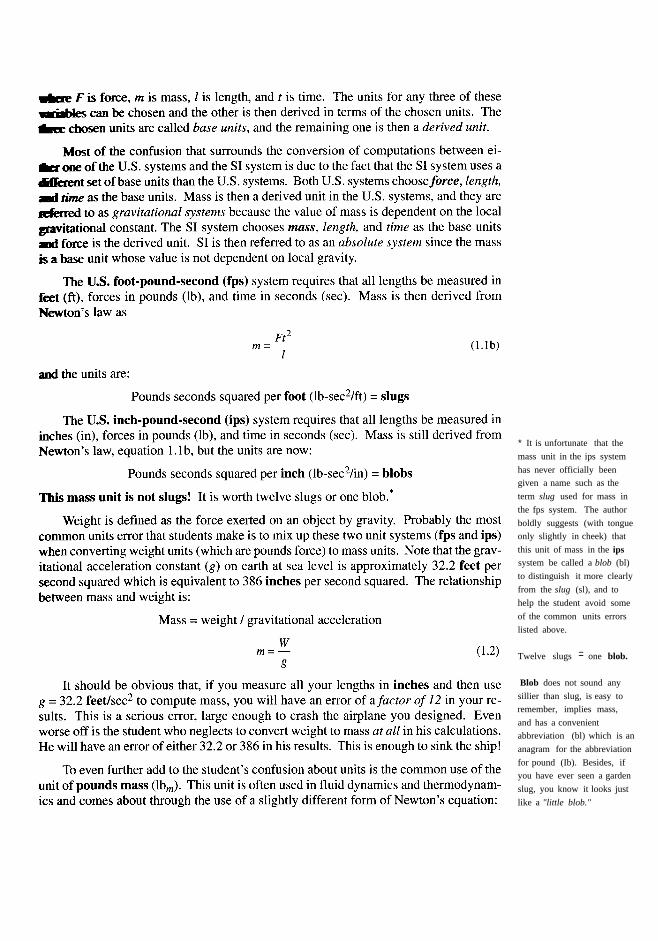
* It is unfortunate that themass unit in the ips systemhas never officially beengiven a name such as theterm slug used for mass inthe fps system. The authorboldly suggests (with tongueonly slightly in cheek) thatthis unit of mass in the ipssystem be called a blob (bl)to distinguish it more clearlyfrom the slug (sl), and tohelp the student avoid someof the common units errorslisted above.
Twelve slugs = one blob.
Blob does not sound anysillier than slug, is easy toremember, implies mass,and has a convenientabbreviation (bl) which is ananagram for the abbreviationfor pound (Ib). Besides, ifyou have ever seen a gardenslug, you know it looks justlike a "little blob."

where m = mass in Ibm' a = acceleration and gc = the gravitational constant.
The value of the mass of an object measured in pounds mass (Ibm) is numericallyequal to its weight in pounds force (Ib/). However the student must remember to dividethe value of m in Ibm by gc when substituting into this form of Newton's equation. Thusthe Ibm will be divided either by 32.2 or by 386 when calculating the dynamic force. Theresult will be the same as when the mass is expressed in either slugs or blobs in the F =ma form of the equation. Remember that in round numbers at sea level on earth:
I Ibm = llbf I slug = 32.2 Ibf I blob = 386 Ibf
The SI system requires that lengths be measured in meters (m), mass in kilograms(kg), and time in seconds (sec). This is sometimes also referred to as the mks system.Force is derived from Newton's law, equation 1.1b and the units are:
kilogram-meters per second2 (kg-m/sec2) = newtons
Thus in the SI system there are distinct names for mass and force which helps alle-viate confusion. When converting between SI and u.s. systems, be alert to the fact thatmass converts from kilograms (kg) to either slugs (sl) or blobs (bl), and force convertsfrom newtons (N) to pounds (Ib). The gravitational constant (g) in the SI system is ap-proximately 9.81 m/sec2.
The principal system of units used in this textbook will be the U.S. ips system. Mostmachine design in the United States is still done in this system. Table 1-4 shows someof the variables used in this text and their units. The inside front cover contains a tableof conversion factors between the U.S, and SI systems.
The student is cautioned to always check the units in any equation written for a prob-lem solution, whether in school or in professional practice after graduation. If properlywritten, an equation should cancel all units across the equal sign. If it does not, then youcan be absolutely sure it is incorrect. Unfortunately, a unit balance in an equation doesnot guarantee that it is correct, as many other errors are possible. Always double-checkyour results. You might save a life.
1.11 WHAT'S TO COME
In this text we will explore the topic of machine design in respect to the synthesis ofmechanisms in order to accomplish desired motions or tasks, and also the analysis ofthese mechanisms in order to determine their rigid-body dynamic behavior. On thepremise that we cannot analyze anything until it has been synthesized into existence, wewill first explore the topic of synthesis of mechanisms. Then we will investigate theanalysis of those and other mechanisms for their kinematic behavior. Finally, in Part IIwe will deal with the dynamic analysis of the forces and torques generated by thesemoving machines. These topics cover the essence of the early stages of a design project.Once the kinematics and kinetics of a design have been determined, most of the concep-tual design will have been accomplished. What then remains is detailed design-sizingthe parts against failure. The topic of detailed design is discussed in other texts such asreference [8].


7 Suh, N. P. (1995). "Axiomatic Design of Mechanical Systems." Journal of Mechani-cal Design, 117b(2), p. 2.
8 Norton, R. L. (1996). Machine Design: An Integrated Approach. Prentice-Hall:Upper Saddle River, NJ.
For additional information on the history of kinematics, the following are recommended:
Artobolevsky, I. I. (1976). "Past Present and Future of the Theory of Machines and Mecha-nisms." Mechanism and Machine Theory, 11, pp. 353-361.
Brown, H. T. (1869). Five Hundred and Seven Mechanical Movements. Brown, Coombs &Co.: New York, republished by USM Corporation, Beverly, MA., 1970.
de Jonge, A. E. R. (1942). "What Is Wrong with 'Kinematics' and 'Mechanisms'?" MechanicalEngineering, 64(April), pp. 273-278.
de Jonge, A. E. R. (\ 943). "A Brief Account of Modem Kinematics." Transactions of theASME, pp. 663-683.
Erdman, A. E., ed. (1993). Modern Kinematics: Developments in the Last Forty Years. WileySeries in Design Engineering, John Wiley & Sons: New York.
Ferguson, E. S. (1962). "Kinematics of Mechanisms from the Time of Watt." United StatesNational Museum Bulletin, 228(27), pp. 185-230.
Freudenstein, F. (1959). "Trends in the Kinematics of Mechanisms." Applied MechanicsReviews, 12(9), September, pp. 587-590.
Hartenberg, R. S., and J. Denavit. (1964). Kinematic Synthesis of Linkages. McGraw-Hill:New York, pp. 1-27.
Nolle, H. (1974). "Linkage Coupler Curve Synthesis: A Historical Review - II. Developmentsafter 1875." Mechanism and Machine Theory, 9, pp. 325 - 348.
Nolle, H. (1974). "Linkage Coupler Curve Synthesis: A Historical Review -I. Developments upto 1875." Mechanism and Machine Theory, 9, pp. 147-168.
Nolle, H. (\ 975). "Linkage Coupler Curve Synthesis: A Historical Review - III. SpatialSynthesis and Optimization." Mechanism and Machine Theory, 10, pp. 41-55.
Reuleaux, F. (1963). The Kinematics of Machinery, A. B. W. Kennedy, translator. DoverPublications: New York, pp. 29-55.
Strandh, S. (1979). A History of the Machine. A&W Publishers: New York.
For additional information on creativity and the design process, the following arerecommended:
Alger, J. R. M., and C. V. Hays. (1964). Creative Synthesis in Design. Prentice-Hall: UpperSaddle River, NJ.
Allen, M. S. (1962). Morphological Creativity. Prentice-Hall: Upper Saddle River, NJ.
Altschuller, G. (1984). Creativity as an Exact Science. Gordon and Breach: New York.
Buhl, H. R. (\960). Creative Engineering Design. Iowa State University Press: Ames, IA.

Dixon. J. R., and C. Poli. (1995). Engineering Design and Design for Manufacturing-AStructured Approach. Field Stone Publishers: Conway, MA.
Fey, V., et aI. (1994). "Application of the Theory ofInventive Problem Solving to Design andManufacturing Systems." CIRP Annals, 43(1), pp. 107-110.
Gordon, W. J. J. (1962). Synectics. Harper & Row: New York.
Haefele, W. J. (1962). Creativity and Innovation. Van Nostrand Reinhold: New York.
Harrisberger, L. (1982). Engineersmanship. Brooks/Cole: Monterey, CA.
Osborn, A. F. (1963). Applied Imagination. Scribners: New York.
Pleuthner, W. (1956). "Brainstorming." Machine Design, January 12, 1956.
Soh, N. P. (1990). The Principles of Design. Oxford University Press: New York.
Taylor, C. W. (1964). Widening Horizons in Creativity. John Wiley & Sons: New York.
Von Fange, E. K. (1959). Professional Creativity. Prentice-Hall: Upper Saddle River, NJ.
For additional information on Human Factors, the following are recommended:
Bailey, R. W. (1982). Human Performance Engineering: A Guidefor System Designers.Prentice-Hall: Upper Saddle River, NJ.
Burgess, W. R. (1986). Designing for Humans: The Human Factor in Engineering. PetrocelliBooks.
Clark, T. S., and E. N. Corlett. (1984). The Ergonomics of Workspaces and Machines. Taylorand Francis.
Huchinson, R. D. (1981). New Horizons for Human Factors in Design. McGraw-Hill: NewYork.
McCormick, D. J. (1964). Human Factors Engineering. McGraw-Hill: New York.
Osborne, D. J. (1987). Ergonomics at Work. John Wiley & Sons: New York.
Pheasant, S. (1986). Bodyspace: Anthropometry, Ergonomics & Design. Taylor and Francis.
Salvendy, G. (1987). Handbook of Human Factors. John Wiley & Sons: New York.
Sanders, M. S. (1987). Human Factors in Engineering and Design. McGraw-Hill: New York.
Woodson, W. E. (1981). Human Factors Design Handbook. McGraw-Hill: New York.
For additional information on writing engineering reports, the following are recommended:
Barrass, R. (1978). Scientists Must Write. John Wiley & Sons: New York.
Crouch, W. G., and R. L. Zetler. (1964). A Guide to Technical Writing. The Ronald Press:New York.
Davis, D. S. (1963). Elements of Engineering Reports. Chemical Publishing Co.: New York.
Gray, D. E. (1963). So You Have to Write a Technical Report. Information Resources Press:Washington, D.C.
Michaelson, H. B. (1982). How to Write and Publish Engineering Papers and Reports. ISIPress: Philadelphia, PA.
Nelson, J. R. (1952). Writing the Technical Report. McGraw-Hill: New York.

22
2.0 INTRODUCTION
This chapter will present definitions of a number of terms and concepts fundamental tothe synthesis and analysis of mechanisms. It will also present some very simple butpowerful analysis tools which are useful in the synthesis of mechanisms.
2.1 DEGREESOF FREEDOM ( DOF)
Any mechanical system can be classified according to the number of degrees of free-dom (DOF) which it possesses. The system's DOF is equal to the number of indepen-dent parameters (measurements) which are needed to uniquely define its position inspace at any instant of time. Note that DOF is defined with respect to a selected frame ofreference. Figure 2-1 shows a pencil lying on a flat piece of paper with an x, y coordi-nate system added. If we constrain this pencil to always remain in the plane of the pa-per, three parameters (DOF) are required to completely define the position of the pencilon the paper, two linear coordinates (x, y) to define the position of anyone point on thepencil and one angular coordinate (8) to define the angle of the pencil with respect to theaxes. The minimum number of measurements needed to define its position are shown inthe figure as x, y, and 8. This system of the pencil in a plane then has three DOF. Notethat the particular parameters chosen to define its position are not unique. Any alternateset of three parameters could be used. There is an infinity of sets of parameters possible,but in this case there must be three parameters per set, such as two lengths and an an-gie, to define the system's position because a rigid body in plane motion has three DOF.

Now allow the pencil to exist in a three-dimensional world. Hold it above yourdesktop and move it about. You now will need six parameters to define its six DOF. Onepossible set of parameters which could be used are three lengths, (x, y, z), plus three an-gles (a, <1>, p). Any rigid body in three-space has six degrees of freedom. Try to identifythese six DOF by moving your pencil or pen with respect to your desktop.
The pencil in these examples represents a rigid body, or link, which for purposes ofkinematic analysis we will assume to be incapable of deformation. This is merely a con-venient fiction to allow us to more easily define the gross motions of the body. We canlater superpose any deformations due to external or inertial loads onto our kinematicmotions to obtain a more complete and accurate picture of the body's behavior. But re-member, we are typically facing a blank sheet of paper at the beginning stage of the de-sign process. We cannot determine deformations of a body until we define its size, shape,material properties, and loadings. Thus, at this stage we will assume, for purposes ofinitial kinematic synthesis and analysis, that our kinematic bodies are rigid andmassless.
2.2 TYPESOF MOTION
A rigid body free to move within a reference frame will, in the general case, have com-plex motion, which is a simultaneous combination of rotation and translation. Inthree-dimensional space, there may be rotation about any axis (any skew axis or one ofthe three principal axes) and also simultaneous translation which can be resolved intocomponents along three axes. In a plane, or two-dimensional space, complex motion be-comes a combination of simultaneous rotation about one axis (perpendicular to the plane)and also translation resolved into components along two axes in the plane. For simplic-ity, we will limit our present discussions to the case of planar (2-0) kinematic systems.We will define these terms as follows for our purposes, in planar motion:

Pure rotationthe body possesses one point (center of rotation) which has no motion with respect to the"stationary" frame of reference. All other points on the body describe arcs about thatcenter. A reference line drawn on the body through the center changes only its angularorientation.
Pure translationall points on the body describe parallel (curvilinear or rectilinear) paths. A reference linedrm\"n on the body changes its linear position but does not change its angular orienta-tion.
Complex motiona simultaneous combination of rotation and translation. Any reference line drawn onthe body will change both its linear position and its angular orientation. Points on thebody will travel nonparallel paths, and there will be, at every instant, a center of rota·tion, which will continuously change location.
Translation and rotation represent independent motions of the body. Each can ex-ist without the other. If we define a 2-D coordinate system as shown in Figure 2-1, the xand y terms represent the translation components of motion, and the e term representsthe rotation component.
2.3 LINKS, JOINTS, AND KINEMATIC CHAINS
We will begin our exploration of the kinematics of mechanisms with an investigation ofthe subject of linkage design. Linkages are the basic building blocks of all mechanisms.We will show in later chapters that all common forms of mechanisms (cams, gears, belts,chains) are in fact variations on a common theme of linkages. Linkages are made up oflinks and joints.
A link, as shown in Figure 2-2, is an (assumed) rigid body which possesses at leasttwo nodes which are points for attachment to other links.
Binary link - one with two nodes.
Ternary link - one with three nodes.
Quaternary link - one with four nodes.

A joint is a connection between two or more links (at their nodes), which allowssome motion, or potential motion, between the connected links. Joints (also called ki-nematic pairs) can be classified in several ways:
1 By the type of contact between the elements, line, point, or surface.
2 By the number of degrees of freedom allowed at the joint.
3 By the type of physical closure of the joint: either force or form closed.
4 By the number of links joined (order of the joint).
Reuleaux [1] coined the term lower pair to describe joints with surface contact (aswith a pin surrounded by a hole) and the term higher pair to describe joints with pointor line contact. However, if there is any clearance between pin and hole (as there mustbe for motion), so-called surface contact in the pin joint actually becomes line contact,as the pin contacts only one "side" of the hole. Likewise, at a microscopic level, a blocksliding on a flat surface actually has contact only at discrete points, which are the tops ofthe surfaces' asperities. The main practical advantage of lower pairs over higher pairs istheir better ability to trap lubricant between their enveloping surfaces. This is especiallytrue for the rotating pin joint. The lubricant is more easily squeezed out of a higher pair,nonenveloping joint. As a result, the pin joint is preferred for low wear and long life,even over its lower pair cousin, the prismatic or slider joint.
Figure 2-3a shows the six possible lower pairs, their degrees of freedom, and theirone-letter symbols. The revolute (R) and the prismatic (P) pairs are the only lower pairsusable in a planar mechanism. The screw (H), cylindric (C), spherical, and flat (F) low-er pairs are all combinations of the revolute and/or prismatic pairs and are used in spatial(3-D) mechanisms. The Rand P pairs are the basic building blocks of all other pairswhich are combinations of those two as shown in Table 2-1.
A more useful means to classify joints (pairs) is by the number of degrees of free-dom that they allow between the two elements joined. Figure 2-3 also shows examplesof both one- and two-freedom joints commonly found in planar mechanisms. Figure 2-3bshows two forms of a planar, one-freedom joint (or pair), namely, a rotating pin joint(R) and a translating slider joint (P). These are also referred to as full joints (i.e., full =1DOF) and are lower pairs. The pin joint allows one rotational DOF, and the slider jointallows one translational DOF between the joined links. These are both contained within(and each is a limiting case of) another common, one-freedom joint, the screw and nut(Figure 2-3a). Motion of either the nut or the screw with respect to the other results inhelical motion. If the helix angle is made zero, the nut rotates without advancing and itbecomes the pin joint. If the helix angle is made 90 degrees, the nut will translate alongthe axis of the screw, and it becomes the slider joint.
Figure 2-3c shows examples of two-freedom joints (h1gherpairs) which simultaneouslyallow two independent, relative motions, namely translation and rotation, between the joinedlinks. Paradoxically, this two-freedom joint is sometimes referred to as a "half joint," withits two freedoms placed in the denominator. The half joint is also called a roll-slide jointbecause it allows both rolling and sliding. A spherical, or ball-and-socket joint (Figure 2-3a),is an example of a three-freedom joint, which allows three independent angular motions be-tween the two links joined. This ball joint would typically be used in a three-dimensionalmechanism, one example being the ball joints in an automotive suspension system.


A joint with more than one freedom may also be a higher pair as shown in Figure2-3c. Full joints (lower pairs) and half joints (higher pairs) are both used in planar (2-D),~ in spatial (3-D) mechanisms. Note that if you do not allow the two links inHgore 2-3c connected by a roll-slide joint to slide, perhaps by providing a high frictioncoefficient between them, you can "lock out" the translating (At) freedom and make itbehave as a full joint. This is then called a pure rolling joint and has rotational freedom(AD) only. A cornmon example of this type of joint is your automobile tire rolling againstdie road, as shown in Figure 2-3e. In normal use there is pure rolling and no sliding atIbis joint, unless, of course, you encounter an icy road or become too enthusiastic aboutaccelerating or cornering. If you lock your brakes on ice, this joint converts to a puresliding one like the slider block in Figure 2-3b. Friction determines the actual numberof freedoms at this kind of joint. It can be pure roll, pure slide, or roll-slide.
To visualize the degree of freedom of a joint in a mechanism, it is helpful to "men-tally disconnect" the two links which create the joint from the rest of the mechanism.You can then more easily see how many freedoms the two joined links have with respectto one another.
Figure 2-3c also shows examples of both form-closed and force-closed joints. Aform-closed joint is kept together or closed by its geometry. A pin in a hole or a slider ina two-sided slot are form closed. In contrast, a force-closed joint, such as a pin in ahalf-bearing or a slider on a surface, requires some external force to keep it together orclosed. This force could be supplied by gravity, a spring, or any external means. Therecan be substantial differences in the behavior of a mechanism due to the choice of forceor form closure, as we shall see. The choice should be carefully considered. In linkag-es, form closure is usually preferred, and it is easy to accomplish. But for cam-followersystems, force closure is often preferred. This topic will be explored further in later chap-ters.
Figure 2-3d shows examples of joints of various orders, where order is defined asthe number of links joined minus one. It takes two links to make a single joint; thus thesimplest joint combination of two links has order one. As additional links are placed onthe same joint, the order is increased on a one for one basis. Joint order has significancein the proper determination of overall degree of freedom for the assembly. We gave def-initions for a mechanism and a machine in Chapter 1. With the kinematic elements oflinks and joints now defined, we can define those devices more carefully based on Reu-leaux's classifications of the kinematic chain, mechanism, and machine. [1]
A kinematic chain is defined as:An assemblage of links and joints, interconnected in a way to provide a controlled out-put motion in response to a supplied input motion.
A mechanism is defined as:A kinematic chain in which at least one link has been "grounded," or attached, to theframe of reference (which itself may be in motion).
A machine is defined as:A combination of resistant bodies arranged to compel the mechanical forces of nature todo work accompanied by determinate motions.

By Reuleaux's definition [1] a machine is a collection of mechanisms arranged totransmit forces and do work. He viewed all energy or force transmitting devices as ma-chines which utilize mechanisms as their building blocks to provide the necessary mo-tion constraints.
We will now define a crank as a link which makes a complete revolution and is piv-oted to ground, a rocker as a link which has oscillatory (back andforth) rotation and ispivoted to ground, and a coupler (or connecting rod) which has complex motion and isnot pivoted to ground. Ground is defined as any link or links that are fixed (nonmov-ing) with respect to the reference frame. Note that the reference frame may in fact itselfbe in motion.
2.4 DETERMINING DEGREE OF FREEDOM
The concept of degree offreedom (DOF) is fundamental to both the synthesis and anal-ysis of mechanisms. We need to be able to quickly determine the DOF of any collectionof links and joints which may be suggested as a solution to a problem. Degree of free-dom (also called the mobility M) of a system can be defined as:
Degree of Freedom
the number of inputs which need to be provided in order to create a predictable output;
also:
the number of independent coordinates required to define its position.
At the outset of the design process, some general definition of the desired outputmotion is usually available. The number of inputs needed to obtain that output mayormay not be specified. Cost is the principal constraint here. Each required input will needsome type of actuator, either a human operator or a "slave" in the fonn of a motor, sole-noid, air cylinder, or other energy conversion device. (These devices are discussed inSection 2.15.) These multiple input devices will have to have their actions coordinatedby a "controller," which must have some intelligence. This control is now often provid-ed by a computer but can also be mechanically programmed into the mechanism design.There is no requirement that a mechanism have only one DOF, although that is oftendesirable for simplicity. Some machines have many DOF. For example, picture the num-ber of control levers or actuating cylinders on a bulldozer or crane. See Figure I-lb(p.7).
Kinematic chains or mechanisms may be either open or closed. Figure 2-4 showsboth open and closed mechanisms. A closed mechanism will have no open attachmentpoints or nodes and may have one or more degrees of freedom. An open mechanism ofmore than one link will always have more than one degree of freedom, thus requiring asmany actuators (motors) as it has DOF. A common example of an open mechanism is anindustrial robot. An open kinematic chain of two binary links and one joint is called adyad. The sets of links shown in Figure 2-3a and b are dyads.
Reuleaux limited his definitions to closed kinematic chains and to mechanisms hav-ing only one DOF, which he called constrained. [1] The somewhat broader definitionsabove are perhaps better suited to current-day applications. A multi-DOF mechanism,such as a robot, will be constrained in its motions as long as the necessary number ofinputs are supplied to control all its DOF.

Degree of Freedom in Planar Mechanisms
To determine the overall DOF of any mechanism, we must account for the number oflinks and joints, and for the interactions among them. The DOF of any assembly of linkscan be predicted from an investigation of the Gruebler condition. [2] Any link in a planebas 3 DOF. Therefore, a system of L unconnected links in the same plane will have 3LDOF, as shown in Figure 2-5a where the two unconnected links have a total of six DOF.When these links are connected by a full joint in Figure 2-5b, ~Yl and ~Y2 are combinedas ~Y, and Lixl and Lix2 are combined as Lix. This removes two DOF, leaving four DOF.In Figure 2-5c the half joint removes only one DOF from the system (because a half jointhas two DOF), leaving the system of two links connected by a half joint with a total offive DOF. In addition, when any link is grounded or attached to the reference frame, allthree of its DOF will be removed. This reasoning leads to Gruebler's equation:
M=3L-2J-3G (2.1a)
where: M = degree offreedom or mobilityL = number of linksJ = number of jointsG = number of grounded links
Note that in any real mechanism, even if more than one link of the kinematic chainis grounded, the net effect will be to create one larger, higher-order ground link, as therecan be only one ground plane. Thus G is always one, and Gruebler's equation becomes:
where: M = degree offreedom or mobilityL = number of linksJl = number of 1DOF (full) jointsJ2 = number of 2 DOF (half) joints

The value of J1 and lz in these equations must still be carefully determined to ac-count for all full, half, and multiple joints in any linkage. Multiple joints count as oneless than the number oflinks joined at that joint and add to the "full" (11) category. TheDOF of any proposed mechanism can be quickly ascertained from this expression beforeinvesting any time in more detailed design. It is interesting to note that this equation hasno information in it about link sizes or shapes, only their quantity. Figure 2-6a shows amechanism with one DOF and only full joints in it.
Figure 2-6b shows a structure with zero DOF and which contains both half and mul-tiple joints. Note the schematic notation used to show the ground link. The ground linkneed not be drawn in outline as long as all the grounded joints are identified. Note alsothe joints labeled "multiple" and "half' in Figure 2-6a and b. As an exercise, computethe DOF of these examples with Kutzbach's equation.
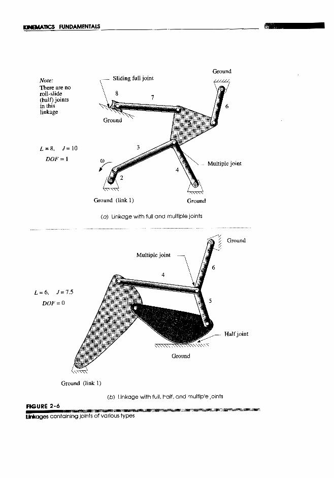

Degree of Freedom in Spatial Mechanisms
The approach used to determine the mobility of a planar mechanism can be easily ex-tended to three dimensions. Each unconnected link in three-space has 6 DOF, and anyone of the six lower pairs can be used to connect them, as can higher pairs with morefreedom. A one-freedom joint removes 5 DOF, a two-freedom joint removes 4 DOF, etc.Grounding a link removes 6 DOF. This leads to the Kutzbach mobility equation for spa-tiallinkages:
* If the sum of the lengthsof any two links is less thanthe length of the third link,then their interconnectionis impossible.
where the subscript refers to the number of freedoms of the joint. We will limit our studyto 2-D mechanisms in this text.
2.5 MECHANISMS AND STRUCTURES
The degree of freedom of an assembly of links completely predicts its character. Thereare only three possibilities. If the DOF is positive, it will be a mechanism, and the linkswill have relative motion. If the DOF is exactly zero, then it will be a structure, and nomotion is possible. If the DOF is negative, then it is a preloaded structure, which meansthat no motion is possible and some stresses may also be present at the time of assembly.Figure 2-7 shows examples of these three cases. One link is grounded in each case.
Figure 2-7a shows four links joined by four full joints which, from the Grueblerequation, gives one DOF. It will move, and only one input is needed to give predictableresults.
Figure 2-7b shows three links joined by three full joints. It has zero DOF and is thusa structure. Note that if the link lengths will allow connection, * all three pins can beinserted into their respective pairs of link holes (nodes) without straining the structure,as a position can always be found to allow assembly.
Figure 2-7c shows two links joined by two full joints. It has a DOF of minus one,making it a preloaded structure. In order to insert the two pins without straining thelinks, the center distances of the holes in both links must be exactly the same. Practical-ly speaking, it is impossible to make two parts exactly the same. There will always besome manufacturing error, even if very small. Thus you may have to force the secondpin into place, creating some stress in the links. The structure will then be preloaded.You have probably met a similar situation in a course in applied mechanics in the formof an indeterminate beam, one in which there were too many supports or constraints forthe equations available. An indeterminate beam also has negative DOF, while a simplysupported beam has zero DOF.
Both structures and preloaded structures are commonly encountered in engineering.In fact the true structure of zero DOF is rare in engineering practice. Most buildings,bridges, and machine frames are preloaded structures, due to the use of welded and riv-eted joints rather than pin joints. Even simple structures like the chair you are sitting inare often preloaded. Since our concern here is with mechanisms, we will concentrate ondevices with positive DOF only.

2.6 NUMBER SYNTHESIS
The term number synthesis has been coined to mean the determination of the numberand order of links and joints necessary to produce motion of a particular DOF. Order inthis context refers to the number of nodes perlink, i.e., binary, ternary, quaternary, etc.The value of number synthesis is to allow the exhaustive determination of all possiblecombinations of links which will yield any chosen DOF. This then equips the designerwith a definitive catalog of potential linkages to solve a variety of motion control prob-lems.
As an example we will now derive all the possible link combinations for one DOF,including sets of up to eight links, and link orders up to and including hexagonal links.For simplicity we will assume that the links will be connected with only full rotatingjoints. We can later introduce half joints, multiple joints, and sliding joints through link-age transformation. First let's look at some interesting attributes of linkages as definedby the above assumption regarding full joints.
Hypothesis: If all joints are full joints, an odd number of DOFrequires an even number of linksand vice versa.
Proof: Given: All even integers can be denoted by 2m or by 2n, and all odd integers canbe denoted by 2m - I or by 2n - 1, where n and m are any positive integers. Thenumber of joints must be a positive integer.
Let: L = number of links, J = number of joints, and M = DOF = 2m (i.e., all even numbers)
Then: rewriting Gruebler's equation (Equation 2.1b) to solve for J,


tion, there are 3 links and 3 full joints, from which Gruebler's equation predicts zeroDOF. However, this linkage does move (actual DOF = 1), because the center distance, orlength of link 1, is exactly equal to the sum of the radii of the two wheels.
There are other examples of paradoxes which disobey the Gruebler criterion due totheir unique geometry. The designer needs to be alert to these possible inconsistencies.
2.8 ISOMERS
The word isomer is from the Greek and means having equal parts. Isomers in chemis-try are compounds that have the same number and type of atoms but which are intercon-nected differently and thus have different physical properties. Figure 2-9a shows twohydrocarbon isomers, n-butane and isobutane. Note that each has the same number ofcarbon and hydrogen atoms (C4HlO), but they are differently interconnected and havedifferent properties.
Linkage isomers are analogous to these chemical compounds in that the links (likeatoms) have various nodes (electrons) available to connect to other links' nodes. Theassembled linkage is analogous to the chemical compound. Depending on the particularconnections of available links, the assembly will have different motion properties. Thenumber of isomers possible from a given collection of links (as in any row of Table 2-2)is far from obvious. In fact the problem of mathematically predicting the number of iso-mers of all link combinations has been a long-unsolved problem. Many researchers havespent much effort on this problem with some recent success. See references [3] through[7] for more information. Dhararipragada [6] presents a good historical summary of iso-mer research to 1994. Table 2-3 shows the number of valid isomers found for one-DOFmechanisms with revolute pairs, up to 12 links.
Figure 2-9b shows all the isomers for the simple cases of one DOF with 4 and 6 links.Note that there is only one isomer for the case of 4 links. An isomer is only unique if theinterconnections between its types of links are different. That is, all binary links areconsidered equal, just as all hydrogen atoms are equal in the chemical analog. Linklengths and shapes do not figure into the Gruebler criterion or the condition of isomer-ism. The 6-link case of 4 binaries and 2 ternaries has only two valid isomers. These areknown as the Watt's chain and the Stephenson's chain after their discoverers. Note thedifferent interconnections of the ternaries to the binaries in these two examples. TheWatt's chain has the two ternaries directly connected, but the Stephenson's chain doesnot.
There is also a third potential isomer for this case of six links, as shown in Figure2-9c, but it fails the test of distribution of degree of freedom, which requires that theoverall DOF (here 1) be uniformly distributed throughout the linkage and not concentrat-ed in a subchain. Note that this arrangement (Figure 2-9c) has a structural subchain ofDOF = 0 in the triangular formation of the two ternaries and the single binary connectingthem. This creates a truss, or delta triplet. The remaining three binaries in series forma fourbar chain (DOF = 1) with the structural subchain of the two ternaries and the singlebinary effectively reduced to a structure which acts like a single link. Thus this arrange-ment has been reduced to the simpler case of the fourbar linkage despite its six bars. Thisis an invalid isomer and is rejected. It is left as an exercise for the reader to find the 16valid isomers of the eight bar, one-DOF cases.


• If all revolute joints in afourbar linkage arereplaced by prismaticjoints, the result will be atwo-DOF assembly. Also,if three revolutes in a four-bar loop are replaced withprismatic joints, the oneremaining revolute jointwill not be able to turn,effectively locking the twopinned links together asone. This effectivelyreduces the assembly to athreebar linkage whichshould have zero DOF.But, a delta triplet withthree prismatic joints hasone DOF-anotherGruebler's paradox.
2.9 LINKAGE TRANSFORMATION
The number synthesis techniques described above give the designer a toolkit of basiclinkages of particular DOF. If we now relax the arbitrary constraint which restricted usto only revolute joints, we can transform these basic linkages to a wider variety of mech-anisms with even greater usefulness. There are several transformation techniques orrules that we can apply to planar kinematic chains.
1 Revolute joints in any loop can be replaced by prismatic joints with no change inDOF of the mechanism, provided that at least two revolute joints remain in the loop. *
2 Any full joint can be replaced by a half joint, but this will increase the DOF by one.
3 Removal of a link will reduce the DOF by one.
4 The combination of rules 2 and 3 above will keep the original DOF unchanged.
5 Any ternary or higher-order link can be partially "shrunk" to a lower-order link bycoalescing nodes. This will create a multiple joint but will not change the DOF ofthe mechanism.
6 Complete shrinkage of a higher-order link is equivalent to its removal. A multiplejoint will be created, and the DOF will be reduced.
Figure 2-lOa shows a fourbar crank-rocker linkage transformed into the fourbarslider-crank by the application of rule #1. It is still a fourbar linkage. Link 4 has be-come a sliding block. The Gruebler's equation is unchanged at one DOF because the slid-er block provides a full joint against link 1, as did the pin joint it replaces. Note that thistransformation from a rocking output link to a slider output link is equivalent to increas-ing the length (radius) of rocker link 4 until its arc motion at the joint between links 3and 4 becomes a straight line. Thus the slider block is equivalent to an infinitely longrocker link 4, which is pivoted at infinity along a line perpendicular to the slider axis asshown in Figure 2-lOa.
Figure 2-lOb shows a fourbar slider-crank transformed via rule #4 by the substitu-tion of a half joint for the coupler. The first version shown retains the same motion ofthe slider as the original linkage by use of a curved slot in link 4. The effective coupler
. is always perpendicular to the tangent of the slot and falls on the line of the original cou-pler. The second version shown has the slot made straight and perpendicular to the slid-er axis. The effective coupler now is "pivoted" at infinity. This is called a Scotch yokeand gives exact simple harmonic motion of the slider in response to a constant speed in-put to the crank.
Figure 2-lOc shows a fourbar linkage transformed into a earn-follower linkage bythe application of rule #4. Link 3 has been removed and a half joint substituted for a fulljoint between links 2 and 4. This still has one DOF, and the cam-follower is in fact afourbar linkage in another disguise, in which the coupler (link 3) has become an effec-tive link of variable length. We will investigate the fourbar linkage and these variants ofit in greater detail in later chapters.
Figure 2-lla shows the Stephenson's sixbar chain from Figure 2-9b (p. 39) trans-formed by partial shrinkage of a ternary link (rule #5) to create a multiple joint. It isstill a one-DOF Stephenson's sixbar. Figure 2-11 b shows the Watt's sixbar chain from


Figure 2-9b with one ternary link completely shrunk to create a multiple joint. This isnow a structure with DOF = O. The two triangular subchains are obvious. Just as thefourbar chain is the basic building block of one-DOF mechanisms, this threebar triangledelta triplet is the basic building block of zero-DOF structures (trusses).
2.10 INTERMITTENT MOTION
Intermittent motion is a sequence of motions and dwells. A dwell is a period in whichthe output link remains stationary while the input link continues to move. There are manyapplications in machinery which require intermittent motion. The earn-follower varia-tion on the fourbar linkage as shown in Figure 2-lOc (p. 41) is often used in these situa-tions. The design of that device for both intermittent and continuous output will be ad-dressed in detail in Chapter 8. Other pure linkage dwell mechanisms are discussed inthe next chapter.
GENEVAMECHANISM A common form of intermittent motion device is the Gene-va mechanism shown in Figure 2-12a. This is also a transformed fourbar linkage inwhich the coupler has been replaced by a half joint. The input crank (link 2) is typicallymotor driven at a constant speed. The Geneva wheel is fitted with at least three equis-paced, radial slots. The crank has a pin that enters a radial slot and causes the Genevawheel to turn through a portion of a revolution. When the pin leaves that slot, the Gene-va wheel remains stationary until the pin enters the next slot. The result is intermittentrotation of the Geneva wheel.
The crank is also fitted with an arc segment, which engages a matching cutout onthe periphery of the Geneva wheel when the pin is out of the slot. This keeps the Gene-va wheel stationary and in the proper location for the next entry of the pin. The numberof slots determines the number of "stops" of the mechanism, where stop is synonymous

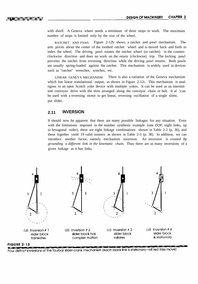
with dwell. A Geneva wheel needs a minimum of three stops to work. The maximumnumber of stops is limited only by the size of the wheel.
RATCHET AND PAWL Figure 2-12b shows a ratchet and pawl mechanism. Thearm pivots about the center of the toothed ratchet wheel and is moved back and forth toindex the wheel. The driving pawl rotates the ratchet wheel (or ratchet) in the counter-clockwise direction and does no work on the return (clockwise) trip. The locking pawlprevents the ratchet from reversing direction while the driving pawl returns. Both pawlsare usually spring-loaded against the ratchet. This mechanism is widely used in devicessuch as "ratchet" wrenches, winches, etc.
LINEAR GENEVA MECHANISM There is also a variation of the Geneva mechanismwhich has linear translational output, as shown in Figure 2-12c. This mechanism is anal-ogous to an open Scotch yoke device with multiple yokes. It can be used as an intermit-tent conveyor drive with the slots arranged along the conveyor chain or belt. It al 'r;anbe used with a reversing motor to get linear, reversing oscillation of a single slotte,put slider.
2.11 INVERSION
It should now be apparent that there are many possible linkages for any situation. Evenwith the limitations imposed in the number synthesis example (one DOF, eight links, upto hexagonal order), there are eight linkage combinations shown in Table 2-2 (p. 36), andthese together yield 19 valid isomers as shown in Table 2-3 (p. 38). In addition, we canintroduce another factor, namely mechanism inversion. An inversion is created bygrounding a different link in the kinematic chain. Thus there are as many inversions of agiven linkage as it has links.
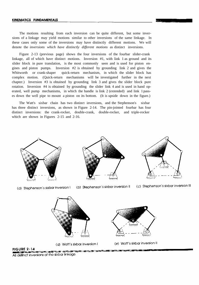
The motions resulting from each inversion can be quite different, but some inver-sions of a linkage may yield motions similar to other inversions of the same linkage. Inthese cases only some of the inversions may have distinctly different motions. We willdenote the inversions which have distinctly different motions as distinct inversions.
Figure 2-13 (previous page) shows the four inversions of the fourbar slider-cranklinkage, all of which have distinct motions. Inversion #1, with link 1 as ground and itsslider block in pure translation, is the most commonly seen and is used for piston en-gines and piston pumps. Inversion #2 is obtained by grounding link 2 and gives theWhitworth or crank-shaper quick-return mechanism, in which the slider block hascomplex motion. (Quick-return mechanisms will be investigated further in the nextchapter.) Inversion #3 is obtained by grounding link 3 and gives the slider block purerotation. Inversion #4 is obtained by grounding the slider link 4 and is used in hand op-erated, well pump mechanisms, in which the handle is link 2 (extended) and link 1 pass-es down the well pipe to mount a piston on its bottom. (It is upside down in the figure.)
The Watt's sixbar chain has two distinct inversions, and the Stephenson's sixbarhas three distinct inversions, as shown in Figure 2-14. The pin-jointed fourbar has fourdistinct inversions: the crank-rocker, double-crank, double-rocker, and triple-rockerwhich are shown in Figures 2-15 and 2-16.

2.12 THE GRASHOF CONDITION
The fourbar linkage has been shown above to be the simplest possible pin-jointed mech-anism for single degree of freedom controlled motion. It also appears in various disguis-es such as the slider-crank and the earn-follower. It is in fact the most common andubiquitous device used in machinery. It is also extremely versatile in terms of the typesof motion which it can generate.
Simplicity is one mark of good design. The fewest parts that can do the job will usu-ally give the least expensive and most reliable solution. Thus the fourbar linkage shouldbe among the first solutions to motion control problems to be investigated. The Grashofcondition [8] is a very simple relationship which predicts the rotation behavior or rotat-ability of a fourbar linkage's inversions based only on the link lengths.
Let: S = length of shortest linkL = length of longest link

P = length of one remaining linkQ = length of other remaining link
Then if : (2.8)
the linkage is Grashof and at least one link will be capable of making a full revolutionwith respect to the ground plane. This is called a Class I kinematic chain. If the inequality isnot true, then the linkage is non-Grashof and no link will be capable of a complete rev-olution relative to any other link. This is a Class II kinematic chain.
Note that the above statements apply regardless of the order of assembly of the links.That is, the determination of the Grashof condition can be made on a set of unassembledlinks. Whether they are later assembled into a kinematic chain in S, L, P, Q, or S, P, L, Qor any other order, will not change the Grashof condition.
The motions possible from a fourbar linkage will depend on both the Grashof con-dition and the inversion chosen. The inversions will be defined with respect to the short-est link. The motions are:

For the Class I case, S + L <P + Q:
Ground either link adjacent to the shortest and you get a crank-rocker, in which theshortest link will fully rotate and the other link pivoted to ground will oscillate.
Ground the shortest link and you will get a double-crank, in which both links piv-oted to ground make complete revolutions as does the coupler.
Ground the link opposite the shortest and you will get a Grashof double-rocker, inwhich both links pivoted to ground oscillate and only the coupler makes a full revolu-tion.
For the Class II case, S + L > P + Q:
All inversions will be triple-rockers [9] in which no link can fully rotate.
For the Class III case, S + L = P + Q:
Referred to as special-case Grashof and also as a Class IIIkinematic chain, all in-versions will be either double-cranks or crank-rockers but will have "change points"twice per revolution of the input crank when the links all become colinear. At thesechange points the output behavior will become indeterminate. The linkage behavior isthen unpredictable as it may assume either of two configurations. Its motion must be lim-ited to avoid reaching the change points or an additional, out-of-phase link provided toguarantee a "carry through" of the change points. (See Figure 2-17 c.)
Figure 2-15 (p. 46) shows the four possible inversions of the Grashof case: twocrank-rockers, a double-crank (also called a drag link), and a double-rocker with rotat-ing coupler. The two crank-rockers give similar motions and so are not distinct from oneanother. Figure 2-16 (p. 47) shows four non-distinct inversions, all triple-rockers, of anon-Grashof linkage.
Figure 2-17 a and b shows the parallelogram and antiparallelogram configurationsof the special-case Grashof linkage. The parallelogram linkage is quite useful as it ex-actly duplicates the rotary motion of the driver crank at the driven crank. One commonuse is to couple the two windshield wiper output rockers across the width of the wind-shield on an automobile. The coupler of the parallelogram linkage is in curvilinear trans-lation, remaining at the same angle while all points on it describe identical circular paths.It is often used for this parallel motion, as in truck tailgate lifts and industrial robots.
The antiparallelogram linkage is also a double-crank, but the output crank has anangular velocity different from the input crank. Note that the change points allow thelinkage to switch unpredictably between the parallelogram and anti parallelogram formsevery 180 degrees unless some additional links are provided to carry it through thosepositions. This can be achieved by adding an out-of-phase companion linkage coupledto the same crank, as shown in Figure 2-17c. A common application of this double par-allelogram linkage was on steam locomotives, used to connect the drive wheels togeth-er. The change points were handled by providing the duplicate linkage, 90 degrees outof phase, on the other side of the locomotive's axle shaft. When one side was at a changepoint, the other side would drive it through.
The double-parallelogram arrangement shown in Figure 2-17 c is quite useful as itgives a translating coupler which remains horizontal in all positions. The two parallelo-

gram stages of the linkage are out of phase so each carries the other through its changepoints. Figure 2-17d shows the deltoid or kite configuration which is a crank-rocker.
There is nothing either bad or good about the Grashof condition. Linkages of allthree persuasions are equally useful in their place. If, for example, your need is for amotor driven windshield wiper linkage, you may want a non-special-case Grashof crank-rocker linkage in order to have a rotating link for the motor's input, plus a special-caseparallelogram stage to couple the two sides together as described above. If your need isto control the wheel motions of a car over bumps, you may want a non-Grashof triple-rocker linkage for short stroke oscillatory motion. If you want to exactly duplicate someinput motion at a remote location, you may want a special-case Grashof parallelogramlinkage, as used in a drafting machine. In any case, this simply determined condition tellsvolumes about the behavior to be expected from a proposed fourbar linkage design prior10 any construction of models or prototypes.


rocker requires adding a flywheel to the crank as is done with the internal combustionengine's slider-crank mechanism (which is a GPRC) linkage. See Figure 2-lOa (p. 41).
Barker also defines a "solution space" whose axes are the link ratios Ai, A3, "-4 asshown in Figure 2-18. These ratios' values theoretically extend to infinity, but for anypractical linkages the ratios can be limited to a reasonable value.
In order for the four links to be assembled, the longest link must be shorter than thesum of the other three links,
If L = (S + P + Q), then the links can be assembled but will not move, so this condi-tion provides a criterion to separate regions of no mobility from regions that allow mo-bility within the solution space. Applying this criterion in terms of the three link ratiosdefines four planes of zero mobility which provide limits to the solution space.

2.13 LINKAGES OF MORE THAN FOUR BARS
Geared Fivebar Linkages
We have seen that the simplest one-DOF linkage is the fourbar mechanism. It is an ex-tremely versatile and useful device. Many quite complex motion control problems canbe solved with just four links and four pins. Thus in the interest of simplicity, designersshould always first try to solve their problems with a fourbar linkage. However, therewill be cases when a more complicated solution is necessary. Adding one link and onejoint to form a fivebar (Figure 2-19a) will increase the DOF by one, to two. By adding apair of gears to tie two links together with a new half joint, the DOF is reduced again toone, and the geared fivebar mechanism (GFBM) of Figure 2-19b is created.
The geared fivebar mechanism provides more complex motions than the fourbarmechanism at the expense of the added link and gearset as can be seen in Appendix E.The reader may also observe the dynamic behavior of the linkage shown in Figure 2-19bby running the program FIVEBARprovided with this text and opening the data fileF02-19b.5br. See Appendix A for instructions in running the program. Accept all thedefault values, and animate the linkage.

Sixbar Linkages
We already met the Watt's and Stephenson's sixbar mechanisms. See Figure 2-14 (p. 45).The Watt's sixbar can be thought of as two fourbar linkages connected in series andsharing two links in common. The Stephenson's sixbar can be thought of as two four-bar linkages connected in parallel and sharing two links in common. Many linkages canbe designed by the technique of combining multiple fourbar chains as basic buildingblocks into more complex assemblages. Many real design problems will require solu-tions consisting of more than four bars. Some Watt's and Stephenson's linkages are pro-vided as built-in examples to the program SIXBARsupplied with this text. You may runthat program to observe these linkages dynamically. Select any example from the menu,accept all default responses, and animate the linkages.
Grashof- Type Rotatability Criteria for Higher-Order Linkages
Rotatability is defined as the ability of at least one link in a kinematic chain to make afull revolution with respect to the other links and defines the chain as Class I, II or III.Revolvability refers to a specific link in a chain and indicates that it is one of the linksthat can rotate.
ROTATABILITYOF GEAREDFIVEBARLINKAGES Ting [11] has derived an expres-sion for rotatability of the geared fivebar linkage that is similar to the fourbar's Grashofcriterion. Let the link lengths be designated L1 through L5 in order of increasing length,

Also, if Li is a revolvable link, any link that is not longer than Li will also be revolvable.
Additional theorems and corollaries regarding limits on link motions can be foundin references [12] and [13]. Space does not permit their complete exposition here. Notethat the rules regarding the behavior of geared fivebar linkages and fourbar linkages (theGrashoflaw) stated above are consistent with, and contained within, these general rotat-ability theorems.
2.14 SPRINGS AS LINKS
We have so far been dealing only with rigid links. In many mechanisms and machines,it is necessary to counterbalance the static loads applied to the device. A common exam-

pIe is the hood hinge mechanism on your automobile. Unless you have the (cheap) mod-el with the strut that you place in a hole to hold up the hood, it will probably have eithera fourbar or sixbar linkage connecting the hood to the body on each side. The hood maybe the coupler of a non-Grashof linkage whose two rockers are pivoted to the body. Aspring is fitted between two of the links to provide a force to hold the hood in the openposition. The spring in this case is an additional link of variable length. As long as itcan provide the right amount of force, it acts to reduce the DOF of the mechanism to zero,and holds the system in static equilibrium. However, you can force it to again be a one-DOF system by overcoming the spring force when you pull the hood shut.
Another example, which may now be right next to you, is the ubiquitous adjustablearm desk lamp, shown in Figure 2-20. This device has two springs that counterbalancethe weight of the links and lamp head. If well designed and made, it will remain stableover a fairly wide range of positions despite variation in the overturning moment due tothe lamp head's changing moment arm. This is accomplished by careful design of thegeometry of the spring-link relationships so that, as the spring force changes with in-creasing length, its moment arm also changes in a way that continually balances thechanging moment of the lamp head.
A linear spring can be characterized by its spring constant, k =F / x, where F is forceand x is spring displacement. Doubling its deflection will double the force. Most coilsprings of the type used in these examples are linear. The design of spring-loaded link-ages will be addressed in a later chapter.
2.15 PRACTICAL CONSIDERATIONS
There are many factors that need to be considered to create good-quality designs. Notall of them are contained within the applicable theories. A great deal of art based on ex-perience is involved in design as well. This section attempts to describe a few such prac-tical considerations in machine design.
PIN JOINTS VERSUSSLIDERSAND HALF JOINTS
Proper material selection and good lubrication are the key to long life in any situation,such as a joint, where two materials rub together. Such an interface is called a bearing.Assuming the proper materials have been chosen, the choice of joint type can have a sig-nificant effect on the ability to provide good, clean lubrication over the lifetime of themachine.
REVOLUTE (PIN) JOINTS The simple revolute or pin joint (Figure 2-2Ia) is theclear winner here for several reasons. It is relatively easy and inexpensive to design andbuild a good quality pin joint. In its pure form-a so-called sleeve or journal bearing-the geometry of pin-in-hole traps a lubricant film within its annular interface by capil-lary action and promotes a condition called hydrodynamic lubrication in which the partsare separated by a thin film of lubricant as shown in Figure 2-22. Seals can easily beprovided at the ends of the hole, wrapped around the pin, to prevent loss of the lubricant.Replacement lubricant can be introduced through radial holes into the bearing interface,either continuously or periodically, without disassembly.

A convenient form of bearing for linkage pivots is the commercially availablespherical rod end shown in Figure 2-23. This has a spherical, sleeve-type bearing whichself-aligns to a shaft that may be out of parallel. Its body threads onto the link, allowinglinks to be conveniently made from round stock with threaded ends that allow adjustmentof link length.
Relatively inexpensive ball and roller bearings are commercially available in alarge variety of sizes for revolute joints as shown in Figure 2-24. Some of these bear-ings (principally ball type) can be obtained prelubricated and with end seals. Their roll-ing elements provide low-friction operation and good dimensional control. Note thatrolling-element bearings actually contain higher-joint interfaces (half joints) at each ballor roller, which is potentially a problem as noted below. However, the ability to traplubricant within the roll cage (by end seals) combined with the relatively high rollingspeed of the balls or rollers promotes hydrodynamic lubrication and long life. For moredetailed information on bearings and lubrication, see reference [15].
For revolute joints pivoted to ground, several commercially available bearing typesmake the packaging easier. Pillow blocks and flange-mount bearings (Figure 2-25) areavailable fitted with either rolling-element (ball, roller) bearings or sleeve-type journalbearings. The pillow block allows convenient mounting to a surface parallel to the pinaxis, and flange mounts fasten to surfaces perpendicular to the pin axis.
PRISMATIC (SLIDER) JOINTS require a carefully machined and straight slot or rod(Figure 2-21b). The bearings often must be custom made, though linear ball bearings(Figure 2-26) are commercially available but must be run over hardened and groundshafts. Lubrication is difficult to maintain in any sliding joint. The lubricant is not geo-metrically captured, and it must be resupplied either by running the joint in an oil bath orby periodic manual regreasing. An open slot or shaft tends to accumulate airborne dirtparticles which can act as a grinding compound when trapped in the lubricant. This willaccelerate wear.
HIGHER (HALF) JOINTS such as a round pin in a slot (Figure 2-21c) or acarn-follower joint (Figure 2-lOc, p. 41) suffer even more acutely from the slider's lu-brication problems, because they typically have two oppositely curved surfaces in linecontact, which tend to squeeze any lubricant out of the joint. This type of joint needs tobe run in an oil bath for long life. This requires that the assembly be housed in an expen-sive, oil-tight box with seals on all protruding shafts.

These joint types are all used extensively in machinery with great success. As longas the proper attention to engineering detail is paid, the design can be successful. Somecommon examples of all three joint types can be found in an automobile. The windshieldwiper mechanism is a pure pin-jointed linkage. The pistons in the engine cylinders aretrue sliders and are bathed in engine oil. The valves in the engine are opened and closedby earn-follower (halt) joints which are drowned in engine oil. You probably changeyour engine oil fairly frequently. When was the last time you lubricated your windshieldwiper linkage? Has this linkage (not the motor) ever failed?
Cantilever or Straddle Mount?
Any joint must be supported against the joint loads. Two basic approaches are possibleas shown in Figure 2-27. A cantilevered joint has the pin Goumal) supported only, as acantilever beam. This is sometimes necessary as with a crank that must pass over thecoupler and cannot have anything on the other side of the coupler. However, a cantile

ver beam is inherently weaker (for the same cross section and load) than a straddle-mounted (simply supported) beam. The straddle mounting can avoid applying a bend-ing moment to the links by keeping the forces in the same plane. The pin will feel a bend-ing moment in both cases, but the straddle-mounted pin is in double shear-two crosssections are sharing the load. A cantilevered pin is in single shear. It is good practice touse straddle-mounted joints (whether revolute, prismatic, or higher) wherever possible.If a cantilevered pin must be used, then a commercial shoulder screw that has a hardenedand ground shank as shown in Figure 2-28 can sometimes serve as a pivot pin.
Short Links
It sometimes happens that the required length of a crank is so short that it is not possibleto provide suitably sized pins or bearings at each of its pivots. The solution is to designthe link as an eccentric crank, as shown in Figure 2-29. One pivot pin is enlarged to thepoint that it, in effect, contains the link. The outside diameter of the circular crank be-comes the journal for the moving pivot. The fixed pivot is placed a distance e from thecenter of this circle equal to the required crank length. The distance e is the crank's ec-centricity (the crank length). This arrangement has the advantage of a large surface areawithin the bearing to reduce wear, though keeping the large-diameter journal lubricatedcan be difficult.
Bearing Ratio
The need for straight-line motion in machinery requires extensive use of linear translat-ing slider joints. There is a very basic geometrical relationship called bearing ratio,which if ignored or violated will invariably lead to problems.
The bearing ratio (BR) is defined as the effective length of the slider over the effec-tive diameter of the bearing: BR = L / D. For smooth operation this ratio should begreater than 1.5, and never less than 1. The larger it is, the better. Effective length isdefined as the distance over which the moving slider contacts the stationary guide. Thereneed not be continuous contact over that distance. That is, two short collars, spaced farapart, are effectively as long as their overall separation plus their own lengths and arekinematically equivalent to a long tube. Effective diameter is the largest distanceacross the stationary guides, in any plane perpendicular to the sliding motion.

If the slider joint is simply a rod in a bushing, as shown in Figure 2-30a, the effec-tive diameter and length are identical to the actual dimensions of the rod diameter andbushing length. If the slider is a platform riding on two rods and multiple bushings, asshown in Figure 2-30b, then the effective diameter and length are the overall width andlength, respectively, of the platform assembly. It is this case that often leads to poor bear-ing ratios.
A common example of a device with a poor bearing ratio is a drawer in an inexpen-sive piece of furniture. If the only guides for the drawer's sliding motion are its sidesrunning against the frame, it will have a bearing ratio less than 1, since it is wider than itis deep. You have probably experienced the sticking and jamming that occurs with sucha drawer. A better-quality chest of drawers will have a center guide with a large L/ Dratio under the bottom of the drawer and will slide smoothly.
Unkages versus Cams
The pin-jointed linkage has all the advantages of revolute joints listed above. Theearn-follower mechanism (Figure 2-lOc, p. 41) has all the problems associated with thehalf joint listed above. But, both are widely used in machine design, often in the samemachine and in combination (cams driving linkages). So why choose one over the other?
The "pure" pin-jointed linkage with good bearings at the joints is a potentially su-perior design, all else equal, and it should be the first possibility to be explored in anymachine design problem. However, there will be many problems in which the need fora straight, sliding motion or the exact dwells of a earn-follower are required. Then thepractical limitations of earn and slider joints will have to be dealt with accordingly.

* The terms motor andengine are often usedinterchangeably, but theydo not mean the samething. Their difference islargely semantic, but the"purist" reserves the termmotor for electrical,hydraulic and pneumaticmotors and the term enginefor thermodynamic devicessuch as steam engines andinternal combustionengines. Thus, yourautomobile is powered byan engine, but itswindshield wipers andwindow lifts are run bymotors.
Linkages have the disadvantage of relatively large size compared to the output dis-placement of the working portion; thus they can be somewhat difficult to package. Camstend to be compact in size compared to the follower displacement. Linkages are rela-tively difficult to synthesize, and cams are relatively easy to design (as long as a com-puter is available). But linkages are much easier and cheaper to manufacture to highprecision than cams. Dwells are easy to get with cams, and difficult with linkages. Link-ages can survive very hostile environments, with poor lubrication, whereas cams cannot,unless sealed from environmental contaminants. Linkages have better high-speed dy-namic behavior than cams, are less sensitive to manufacturing errors, and can handlevery high loads, but cams can match specified motions better.
So the answer is far from clear-cut. It is another design trade-off situation in whichyou must weigh all the factors and make the best compromise. Because of the potentialadvantages of the pure linkage it is important to consider a linkage design before choos-ing a potentially easier design task but an ultimately more expensive solution.
2.16 MOTORS AND DRIVERS
Unless manually operated, a mechanism will require some type of driver device to pro-vide the input motion and energy. There are many possibilities. If the design requires acontinuous rotary input motion, such as for a Grashof linkage, a slider-crank, or acam-follower, then a motor or engine* is the logical choice. Motors come in a wide va-riety of types. The most common energy source for a motor is electricity, but compressedair and pressurized hydraulic fluid are also used to power air and hydraulic motors.Gasoline or diesel engines are another possibility. If the input motion is translation, asis common in earth-moving equipment, then a hydraulic or pneumatic cylinder is usual-ly needed.
Electric Motors
Electric motors are classified both by their function or application and by their electricalconfiguration. Some functional classifications (described below) are gearmotors, ser-vomotors, and stepping motors. Many different electrical configurations as shown inFigure 2-31 are also available, independent of their functional classifications. The mainelectrical configuration division is between AC and DC motors, though one type, theuniversal motor is designed to run on either AC or DC.
AC and DC refer to alternating current and direct current respectively. AC is typ-ically supplied by the power companies and, in the U. S., will be alternating sinusoidallyat 60 hertz (Hz), at about ±120, ±240, or ±480 volts (V) peak. Many other countriessupply AC at 50 Hz. Single-phase AC provides a single sinusoid varying with time, and3-phase AC provides three sinusoids at 1200 phase angles. DC current is constant withtime, supplied from generators or battery sources and is most often used in vehicles, suchas ships, automobiles, aircraft, etc. Batteries are made in multiples of 1.5 V, with 6, 12,and 24 V being the most common. Electric motors are also classed by their rated poweras shown in Table 2-5. Both AC and DC motors are designed to provide continuous ro-tary output. While they can be stalled momentarily against a load, they can not toleratea full-current, zero-velocity stall for more than a few minutes without overheating.

DC MOTORS are made in different electrical configurations, such as permanentmagnet (PM), shunt-wound, series-wound, and compound-wound. The names refer tothe manner in which the rotating armature coils are electrically connected to the station-ary field coils-in parallel (shunt), in series, or in combined series-parallel (compound).Permanent magnets replace the field coils in a PM motor. Each configuration providesdifferent torque-speed characteristics. The torque-speed curve of a motor describes howit will respond to an applied load and is of great interest to the mechanical designer as itpredicts how the mechanical-electrical system will behave when the load varies dynam-ically with time.
PERMANENT MAGNET DC MOTORS Figure 2-32a shows a torque-speed curve fora permanent magnet (PM) motor. Note that its torque varies greatly with speed, rangingfrom a maximum (stall) torque at zero speed to zero torque at maximum (no-load) speed.This relationship comes from the fact that power = torque X angular velocity. Since thepower available from the motor is limited to some finite value, an increase in torque re-quires a decrease in angular velocity and vice versa. Its torque is maximum at stall (zerovelocity), which is typical of all electric motors. This is an advantage when startingheavy loads: e.g., an electric-motor-powered vehicle needs no clutch, unlike one pow-ered by an internal combustion engine which cannot start from stall under load. An en-gine's torque increases rather than decreases with increasing angular velocity.
Figure 2-32b shows a family of load lines superposed on the torque-speed curve ofa PM motor. These load lines represent a time-varying load applied to the driven mech-anism. The problem comes from the fact that as the required load torque increases, themotor must reduce speed to supply it. Thus, the input speed will vary in response to load

variations in most motors, regardless of their design. * If constant speed is required, thismay be unacceptable. Other types of DC motors have either more or less speed sensitiv-ity to load than the PM motor. A motor is typically selected based on its torque-speedcurve.
SHUNT-WOUND DC MOTORS have a torque speed curve like that shown in Fig-ure 2-33a. Note the flatter slope around the rated torque point (at 100%) compared toFigure 2-32. The shunt-wound motor is less speed-sensitive to load variation in its oper-ating range, but stalls very quickly when the load exceeds its maximum overload capac-ity of about 250% of rated torque. Shunt-wound motors are typically used on fans andblowers.
SERIES-WOUND DC MOTORS have a torque-speed characteristic like that shownin Figure 2-33b. This type is more speed-sensitive than the shunt or PM configurations.However, its starting torque can be as high as 800% of full-load rated torque. It also doesnot have any theoretical maximum no-load speed which makes it tend to run away if theload is removed. Actually, friction and windage losses will limit its maximum speedwhich can be as high as 20,000 to 30,000 revolutions per minute (rpm). Overspeed de-tectors are sometimes fitted to limit its unloaded speed. Series-wound motors are usedin sewing machines and portable electric drills where their speed variability can be anadvantage as it can be controlled, to a degree, with voltage variation. They are also usedin heavy-duty applications such as vehicle traction drives where their high starting torqueis an advantage. Also their speed sensitivity (large slope) is advantageous in high-loadapplications as it gives a "soft-start" when moving high-inertia loads. The motor's ten-dency to slow down when the load is applied cushions the shock that would be felt if alarge step in torque were suddenly applied to the mechanical elements.
COMPOUND-WOUND DC MOTORS have their field and armature coils connectedin a combination of series and parallel. As a result their torque-speed characteristic hasaspects of both the shunt-wound and series-wound motors as shown in Figure 2-33c.

1beir speed sensitivity is greater than a shunt-wound but less than a series-wound motorand it will not run away when unloaded. This feature plus its high starting torque andsoft-start capability make it a good choice for cranes and hoists which experience highinertial loads and can suddenly lose the load due to cable failure, creating a potential run-away problem if the motor does not have a self-limited no-load speed.
SPEED-CONTROLLEDDC MOTORS If precise speed control is needed, as is oftenthe case in production machinery, another solution is to use a speed-controlled DC mo-tor which operates from a controller that increases and decreases the current to the mo-tor in the face of changing load to try to maintain constant speed. These speed-controlled(typically PM) DC motors will run from an AC source since the controller also convertsAC to DC. The cost of this solution is high, however. Another possible solution is toprovide a flywheel on the input shaft, which will store kinetic energy and help smoothout the speed variations introduced by load variations. Flywheels will be investigated inChapter 11.
AC MOTORS are the least expensive way to get continuous rotary motion, andthey can be had with a variety of torque-speed curves to suit various load applications.They are limited to a few standard speeds that are a function of the AC line frequency(60 Hz in North America, 50 Hz elsewhere). The synchronous motor speed ns is a func-tion of line frequency f and the number of magnetic poles p present in the rotor.
(2.17)
Synchronous motors "lock on" to the AC line frequency and run exactly at synchronousspeed. These motors are used for clocks and timers. Nonsynchronous AC motors havea small amount of slip which makes them lag the line frequency by about 3 to 10%.
Table 2-6 shows the synchronous and non synchronous speeds for various AC mo-tor-pole configurations. The most common AC motors have 4 poles, giving nonsynchro-

nous no-load speeds of about 1725 rpm, which reflects slippage from the 60-Hz synchro-nous speed of 1800 rpm.
Figure 2-34 shows typical torque-speed curves for single-phase (1<\»and 3-phase(3<\»AC motors of various designs. The single-phase shaded pole and permanent splitcapacitor designs have a starting torque lower than their full-load torque. To boost thestart torque, the split-phase and capacitor-start designs employ a separate starting circuitthat is cut off by a centrifugal switch as the motor approaches operating speed. The bro-ken curves indicate that the motor has switched from its starting circuit to its runningcircuit. The NEMA * three-phase motor designs B, C, and D in Figure 2-34 differ main-ly in their starting torque and in speed sensitivity (slope) near the full-load point.
GEARMOTORS If different single (as opposed to variable) output speeds than thestandard ones of Table 2-6 are needed, a gearbox speed reducer can be attached to themotor's output shaft, or a gearmotor can be purchased that has an integral gearbox. Gear-motors are commercially available in a large variety of output speeds and power ratings.The kinematics of gearbox design are covered in Chapter 9.
SERVOMOTORS are fast-response, closed-loop-controlled motors capable of pro-viding a programmed function of acceleration or velocity, as well as of holding a fixedposition against a load. Closed loop means that sensors on the output device beingmoved feed back information on its position, velocity, and acceleration. Circuitry in themotor controller responds to the fed back information by reducing or increasing (or re-versing) the current flow to the motor. Precise positioning of the output device is thenpossible, as is control of the speed and shape of the motor's response to changes in loador input commands. These are very expensive devices which are commonly used in ap-plications such as moving the flight control surfaces in aircraft and guided missiles, andin controlling robots, for example. Servomotors have lower power and torque capacitythan is available from non servo AC or DC motors.

STEPPER MOTORS are designed to position an output device. Unlike ser-vomotors, these run open loop, meaning they receive no feedback as to whether the out-put device has responded as requested. Thus they can get out of phase with the desiredprogram. They will, however, happily sit energized for an indefinite period, holding theoutput in one position. Their internal construction consists of a number of magneticstrips arranged around the circumference of both the rotor and stator. When energized,the rotor will move one step, to the next magnet, for each pulse received. Thus, theseare intermittent motion devices and do not provide continuous rotary motion like oth-er motors. The number of magnetic strips determines their resolution (typically a fewdegrees per step). They are relatively small compared to AC/DC motors and have lowtorque capacity. They are moderately expensive and require special controllers.
Air and Hydraulic Motors
These have more limited application than electric motors, simply because they requirethe availability of a compressed air or hydraulic source. Both of these devices are lessenergy efficient than the direct electrical to mechanical conversion of electric motors,because of the losses associated with the conversion of the energy first from chemicalor electrical to fluid pressure and then to mechanical form. Every energy conversioninvolves some losses. Air motors find widest application in factories and shops, wherehigh-pressure compressed air is available for other reasons. A common example is theair impact wrench used in automotive repair shops. Although individual air motors andair cylinders are relatively inexpensive, these pneumatic systems are quite expensivewhen the cost of all the ancillary equipment is included. Hydraulic motors are mostoften found within machines or systems such as construction equipment (cranes), air-craft, and ships, where high-pressure hydraulic fluid is provided for many purposes.Hydraulic systems are very expensive when the cost of all the ancillary equipment isincluded.
Air and Hydraulic Cylinders
These are linear actuators (piston in cylinder) which provide a limited stroke, straight-line output from a pressurized fluid flow input of either compressed air or hydraulic flu-id (usually oil). They are the method of choice if you need a linear motion as the input.However, they share the same high cost, low efficiency, and complication factors as list-ed under their air and hydraulic motor equivalents above.
Another problem is that of control. Most motors, left to their own devices, will tendto run at a constant speed. A linear actuator, when subjected to a constant pressure fluidsource, typical of most compressors, will respond with more nearly constant accelera-tion, which means its velocity will increase linearly with time. This can result in severeimpact loads on the driven mechanism when the actuator comes to the end of its strokeat maximum velocity. Servovalve control of the fluid flow, to slow the actuator at theend of its stroke, is possible but is quite expensive.
The most common application of fluid power cylinders is in farm and constructionequipment such as tractors and bulldozers, where open loop (non servo) hydraulic cyl-inders actuate the bucket or blade through linkages. The cylinder and its piston becometwo of the links (slider and track) in a slider-crank mechanism. See Figure I-lb (p. 7).

Solenoids
These are electromechanical (AC or DC) linear actuators which share some of the limi-tations of air cylinders, and they possess a few more of their own. They are energy inef-ficient, are limited to very short strokes (about 2 to 3 cm), develop a force which variesexponentially over the stroke, and deliver high impact loads. They are, however, inex-pensive, reliable, and have very rapid response times. They cannot handle much power,and they are typically used as control or switching devices rather than as devices whichdo large amounts of work on a system.
A common application of solenoids is in camera shutters, where a small solenoid isused to pull the latch and trip the shutter action when you push the button to take the pic-ture. Its nearly instantaneous response is an asset in this application, and very little workis being done in tripping a latch. Another application is in electric door or trunk lockingsystems in automobiles, where the click of their impact can be clearly heard when youturn the key (or press the button) to lock or unlock the mechanism.
1 Reuleaux, F. (1963). The Kinematics of Machinery. A. B. W. Kennedy, translator.Dover Publications: New York, pp. 29-55.
2 Gruebler, M. (1917). Getriebelehre. Springer Verlag: Berlin.
3 Fang, W. E., and F. Freudenstein. (1990). "The Stratified Representation ofMechanisms." Journal of Mechanical Design. 112(4), p. 514.
4 Kim, J. T., and B. M. Kwak. (1992). "An Algorithm of Topological Ordering forUnique Representation of Graphs." Journal of Mechanical Design, 114(1), p. 103.
5 Tang, C. S., and T. Liu. (1993). "The Degree Code-A New Mechanism Identifier."Journal of Mechanical Design, 115(3), p. 627.
6 Dhararipragada, V.R., et al. (1994). "A More Direct Method for StructuralSynthesis of Simple-Jointed Planar Kinematic Chains." Proc. of 23rd BiennialMechanisms Conference, Minneapolis, MI, p. 507.
7 Yadav, J. N., et al. (1995). "Detection of Isomorphism Among Kinematic ChainsUsing the Distance Concept." Journal of Mechanical Design, 117(4).
8 Grashof, F. (1883). Theoretische Maschinenlehre. Vol. 2. Voss: Hamburg.
9 Paul, B. (1979). "A Reassessment of Grashof's Criterion." Journal of MechanicalDesign, 101(3), pp. 515-518.
10 Barker, C. (1985). "A Complete Classification of Planar Fourbar Linkages."Mechanism and Machine Theory, 20(6), pp. 535-554.
11 Ting, K. L. (1993). "Fully Rotatable Geared Fivebar Linkages." Proc. of 3rd AppliedMechanisms and Robotics Conference, Cincinnati, pp. 67-1.
12 Ting, K. L., and Y.W. Liu. (1991). "Rotatability Laws for N-Bar Kinematic Chainsand Their Proof." Journal of Mechanical Design, 113(1), pp. 32-39.
13 Shyu, J. H., and K. L. Ting. (1994). "Invariant Link Rotatability of N-Bar Kinemat-ic Chains." Journal of Mechanical Design, 116(1), p. 343.

14 Miller,W. S., ed. Machine Design Electrical and Electronics Reference Issue. PentonPublishing: Cleveland, Ohio.
15 Norton, R. L. (1998). Machine Design: An IntegratedApproach. Prentice-Hall:Upper Saddle River, NJ.
*2-1 Find three (or other number as assigned) of the following common devices. Sketchcareful kinematic diagrams and find their total degrees of freedom.
a. An automobile hood hinge mechanismb. An automobile hatchback lift mechanismc. An electric can openerd. A folding ironing boarde. A folding card tablef. A folding beach chairg. A baby swingh. A folding baby walkeri. A drafting machinej. A fancy corkscrewk. A windshield wiper mechanism1. A dump truck dump mechanismm. A trash truck dumpster mechanismn. A station wagon tailgate mechanismo. An automobile jackp. A collapsible auto radio antennaq. A record turntable and tone arm
2-2 How many DOF do you have in your wrist and hand combined?
2-3 How many DOF do the following joints have?
a. Your kneeb. Your anklec. Your shoulderd. Your hipe. Your knuckle
2-4 How many DOF do the following have in their normal environment?
a. A submerged submarine b. An earth-orbiting satellitec. A surface ship d. A motorcyclee. The print head in a 9-pin dot matrix computer printerf. The pen in an XY plotter
2-5 Are the joints in Problem 2-3 force closed or form closed?
2-6 Describe the motion of the following items as pure rotation, pure translation, orcomplex planar motion.
a. A windmillb. A bicycle (in the vertical plane, not turning)c. A conventional "double-hung" windowd. The keys on a computer keyboarde. The hand of a clockf. A hockey puck on the ice

g. The pen in an XY plotterh. The print head in a computer printeri. A "casement" window
*2-7 Calculate the DOF of the linkages shown in Figure P2-1.
*2-8 Identify the items in Figure P2-1 as mechanisms, structures, or preloaded structures.
*2-9 Use linkage transformation on the linkage of Figure P2-1a to make it a I-DOFmechanism.
*2-10 Use linkage transformation on the linkage of Figure P2-1d to make it a 2-DOFmechanism.
2-11 Use number synthesis to find all the possible link combinations for 2-DOF, up to 9links, to hexagonal order, using only revolute joints.
2-12 Find all the valid isomers of the eightbar I-DOF link combinations in Table 2-2 (p.36) having:
a. Four binary and four ternary linksb. Five binaries, two ternaries, and one quaternary linkc. Six binaries and two quaternary linksd. Six binaries, one ternary, and one pentagonal link
2-13 Use linkage transformation to create a I-DOF mechanism with two sliding full jointsfrom a Stephenson's sixbar linkage in Figure 2-14a (p. 45).

2-14 Use linkage transformation to create a I-DOF mechanism with one sliding full jointand a half joint from a Stephenson's sixbar linkage in Figure 2-14b.
*2-15 Calculate the Grashof condition of the fourbar mechanisms defined below. Buildcardboard models of the linkages and describe the motions of each inversion. Linklengths are in inches (or double given numbers for centimeters).
a. 2 4.5 7 9b. 2 3.5 7 9c. 2 4.0 6 8
2-16 What type(s) of electric motor would you specify
a. To drive a load with large inertia.b. To minimize variation of speed with load variation.c. To maintain accurate constant speed regardless of load variations.
2-17 Describe the difference between a cam-follower (half) joint and a pin joint.
2-18 Examine an automobile hood hinge mechanism of the type described in Section 2.14.Sketch it carefully. Calculate its DOF and Grashof condition. Make a cardboardmodel. Analyze it with a free-body diagram. Describe how it keeps the hood up.
2-19 Find an adjustable arm desk lamp of the type shown in Figure P2-2. Measure it andsketch it to scale. Calculate its DOF and Grashof condition. Make a cardboardmodel. Analyze it with a free-body diagram. Describe how it keeps itself stable. Arethere any positions in which it loses stability? Why?
2-20 Make kinematic sketches, define the types of all the links and joints, and determinethe DOF of the mechanisms shown in Figure P2-3.
*2-21 Find the DOF of the mechanisms in Figure P2-4.
2-22 Find the Grashof condition and Barker classifications of the mechanisms in FigureP2-4a, b, and d. Scale the diagrams for dimensions.


2-33 Figure P2-14 shows a "pick-and-place" mechanism in combination with a "walkingbeam." Sketch its kinematic diagram, determine its DOF and its type (Le., is it afourbar, a Watts sixbar, a Stephenson's sixbar, an eightbar, or what?) Make acardboard model of all but the conveyor portion and examine its motions. Describewhat it does. (It will help if you xerox the page and enlarge it. Then paste the copieson cardboard and cut out the links.)
2-34 Figure P2-15 shows a power hacksaw, used to cut metal. Sketch its kinematicdiagram, determine its DOF and its type (Le., is it a fourbar, a Watts sixbar, aStephenson's sixbar, an eightbar, or what?) Use reverse linkage transformation todetermine its pure revolute-jointed equivalent linkage.
2-35 Figure P2-16 shows a manual press used to compact powdered materials. Sketch itskinematic diagram, determine its DOF and its type (Le., is it a fourbar, a Wattssixbar, a Stephenson's sixbar, an eightbar, or what?) Use reverse linkage transfor-mation to determine its pure revolute-jointed equivalent linkage.


76
3.0 INTRODUCTION
Most engineering design practice involves a combination of synthesis and analysis.Most engineering courses deal primarily with analysis techniques for various situations.However, one cannot analyze anything until it has been synthesized into existence.Many machine design problems require the creation of a device with particular motioncharacteristics. Perhaps you need to move a tool from position A to position B in a par-ticular time interval. Perhaps you need to trace out a particular path in space to insert apart into an assembly. The possibilities are endless, but a common denominator is oftenthe need for a linkage to generate the desired motions. So, we will now explore somesimple synthesis techniques to enable you to create potential linkage design solutions forsome typical kinematic applications.
3.1 SYNTHESIS
QUALITATIVE SYNTHESIS means the creation of potential solutions in the absence ofa well-defined algorithm which configures or predicts the solution. Since most real de-sign problems will have many more unknown variables than you will have equations todescribe the system's behavior, you cannot simply solve the equations to get a solution.Nevertheless you must work in this fuzzy context to create a potential solution and toalso judge its quality. You can then analyze the proposed solution to determine its via-bility, and iterate between synthesis and analysis, as outlined in the design process, un-til you are satisfied with the result. Several tools and techniques exist to assist you inthis process. The traditional tool is the drafting board, on which you layout, to scale,
multiple orthographic views of the design, and investigate its motions by drawing arcs,showing multiple positions, and using transparent, movable overlays. Computer-aideddrafting (CAD) systems can speed this process to some degree, but you will probablyfind that the quickest way to get a sense of the quality of your linkage design is to modelit, to scale, in cardboard or drafting Mylar® and see the motions directly.
Other tools are available in the form of computer programs such as FOURBAR,FIVE-BAR, SIXBAR,SLIDER, DYNACAM,ENGINE, and MATRIX(all included with this text),some of which do synthesis, but these are mainly analysis tools. They can analyze a trialmechanism solution so rapidly that their dynamic graphical output gives almost instan-taneous visual feedback on the quality of the design. Commercially available programssuch as Working Model* also allow rapid analysis of a proposed mechanical design. Theprocess then becomes one of qualitative design by successive analysis which is reallyan iteration between synthesis and analysis. Very many trial solutions can be examinedin a short time using these Computer-aided engineering (CAE) tools. We will developthe mathematical solutions used in these programs in subsequent chapters in order to pro-vide the proper foundation for understanding their operation. But, if you want to trythese programs to reinforce some of the concepts in these early chapters, you may do so.Appendix A is a manual for the use of these programs, and it can be read at any time.Reference will be made to program features which are germane to topics in each chap-ter, as they are introduced. Data files for input to these computer programs are also pro-vided on disk for example problems and figures in these chapters. The data file namesare noted near the figure or example. The student is encouraged to input these sample filesto the programs in order to observe more dynamic examples than the printed page can pro-vide. These examples can be run by merely accepting the defaults provided for all inputs.
TYPE SYNTHESIS refers to the definition of the proper type of mechanism best suit-ed to the problem and is a form of qualitative synthesis.t This is perhaps the most diffi-cult task for the student as it requires some experience and knowledge of the varioustypes of mechanisms which exist and which also may be feasible from a performanceand manufacturing standpoint. As an example, assume that the task is to design a deviceto track the straight-line motion of a part on a conveyor belt and spray it with a chemicalcoating as it passes by. This has to be done at high, constant speed, with good accuracyand repeatability, and it must be reliable. Moreover, the solution must be inexpensive.Unless you have had the opportunity to see a wide variety of mechanical equipment, youmight not be aware that this task could conceivably be accomplished by any of the fol-lowing devices:
- A straight-line linkage- A carn and follower- An air cylinder- A hydraulic cylinder- A robot- A solenoid
Each of these solutions, while possible, may not be optimal or even practical. Moredetail needs to be known about the problem to make that judgment, and that detail willcome from the research phase of the design process. The straight-line linkage may proveto be too large and to have undesirable accelerations; the cam and follower will be ex-pensive, though accurate and repeatable. The air cylinder itself is inexpensive but isnoisy and unreliable. The hydraulic cylinder is more expensive, as is the robot. The so-
* ThestudentversionofWorking Model is includedonCD-ROMwiththisbook.TheprofessionalversionisavailablefromKnowledgeRevolutionInc.,SanMateoCA94402, (800) 766-6615
t AgooddiscussionoftypesynthesisandanextensivebibliographyonthetopiccanbefoundinOlson,D.G.,etal.(1985)."ASystematicProcedureforTypeSynthesisofMechanismswithLiteratureReview."Mechanism andMachine Theory, 20(4), pp.285-295.

* Available fromKnowledge Revolution Inc.,San Mateo CA 94402,(800) 766-6615.
lenoid, while cheap, has high impact loads and high impact velocity. So, you can seethat the choice of device type can have a large effect on the quality of the design. A poorchoice at the type synthesis stage can create insoluble problems later on. The designmight have to be scrapped after completion, at great expense. Design is essentially anexercise in trade-offs. Each proposed type of solution in this example has good and badpoints. Seldom will there be a clear-cut, obvious solution to a real engineering designproblem. It will be your job as a design engineer to balance these conflicting featuresand find a solution which gives the best trade-off of functionality against cost, reliabili-ty, and all other factors of interest. Remember, an engineer can do, with one dollar, whatany fool can do for ten dollars. Cost is always an important constraint in engineeringdesign.
QUANTITATIVESYNTHESIS,OR ANALYTICALSYNTHESIS means the generationof one or more solutions of a particular type which you know to be suitable to the prob-lem, and more importantly, one for which there is a synthesis algorithm defined. As thename suggests, this type of solution can be quantified, as some set of equations existswhich will give a numerical answer. Whether that answer is a good or suitable one isstill a matter for the judgment of the designer and requires analysis and iteration to opti-mize the design. Often the available equations are fewer than the number of potentialvariables, in which case you must assume some reasonable values for enough unknownsto reduce the remaining set to the number of available equations. Thus some qualitativejudgment enters into the synthesis in this case as well. Except for very simple cases, aCAE tool is needed to do quantitative synthesis. One example of such a tool is the pro-gram LlNCAGES,* by A. Erdman et aI., of the University of Minnesota [1] which solvesthe three-position and four-position linkage synthesis problems. The computer programsprovided with this text also allow you to do three-position analytical synthesis and gen-eral linkage design by successive analysis. The fast computation of these programs al-lows one to analyze the performance of many trial mechanism designs in a short timeand promotes rapid iteration to a better solution.
DIMENSIONALSYNTHESIS of a linkage is the determination of the proportions(lengths) of the links necessary to accomplish the desired motions and can be a form ofquantitative synthesis if an algorithm is defined for the particular problem, but can alsobe a form of qualitative synthesis if there are more variables than equations. The lattersituation is more common for linkages. (Dimensional synthesis of cams is quantitative.)Dimensional synthesis assumes that, through type synthesis, you have already deter-mined that a linkage (or a cam) is the most appropriate solution to the problem. Thischapter discusses graphical dimensional synthesis of linkages in detail. Chapter 5 pre-sents methods of analytical linkage synthesis, and Chapter 8 presents cam synthesis.
3.2 FUNCTION, PATH, AND MOTION GENERATION
FUNCTIONGENERATION is defined as the correlation of an input motion with an out-put motion in a mechanism. A function generator is conceptually a "black box" whichdelivers some predictable output in response to a known input. Historically, before theadvent of electronic computers, mechanical function generators found wide applicationin artillery rangefinders and shipboard gun aiming systems, and many other tasks. Theyare, in fact, mechanical analog computers. The development of inexpensive digitalelectronic microcomputers for control systems coupled with the availability of compact

servo and stepper motors has reduced the demand for these mechanical function genera-tor linkage devices. Many such applications can now be served more economically andefficiently with electromechanical devices. * Moreover, the computer-controlled electro-mechanical function generator is programmable, allowing rapid modification of the func-tion generated as demands change. For this reason, while presenting some simple ex-amples in this chapter and a general, analytical design method in Chapter 5, we will notemphasize mechanical linkage function generators in this text. Note however that thecam-follower system, discussed extensively in Chapter 8, is in fact a form of mechani-cal function generator, and it is typically capable of higher force and power levels perdollar than electromechanical systems.
PATH GENERATION is defined as the control of a point in the plane such that itfollows some prescribed path. This is typically accomplished with at least four bars,wherein a point on the coupler traces the desired path. Specific examples are presentedin the section on coupler curves below. Note that no attempt is made in path generationto control the orientation of the link which contains the point of interest. However, it iscommon for the timing of the arrival of the point at particular locations along the path tobe defined. This case is called path generation with prescribed timing and is analogousto function generation in that a particular output function is specified. Analytical pathand function generation will be dealt with in Chapter 5.
MOTION GENERATION is defined as the control of a line in the plane such that itassumes some prescribed set of sequential positions. Here orientation of the link con-taining the line is important. This is a more general problem than path generation, andin fact, path generation is a subset of motion generation. An example of a motion gener-ation problem is the control of the "bucket" on a bulldozer. The bucket must assume aset of positions to dig, pick up, and dump the excavated earth. Conceptually, the motionof a line, painted on the side of the bucket, must be made to assume the desired positions.A linkage is the usual solution.
PLANARMECHANISMSVERSUSSPATIALMECHANISMS The above discussion ofcontrolled movement has assumed that the motions desired are planar (2-D). We live ina three-dimensional world, however, and our mechanisms must function in that world.Spatial mechanisms are 3-D devices. Their design and analysis is much more complexthan that of planar mechanisms, which are 2-D devices. The study of spatial mecha-nisms is beyond the scope of this introductory text. Some references for further studyare in the bibliography to this chapter. However, the study of planar mechanisms is notas practically limiting as it might first appear since many devices in three dimensions areconstructed of multiple sets of 2-D devices coupled together. An example is any foldingchair. It will have some sort of linkage in the left side plane which allows folding. Therewill be an identical linkage on the right side of the chair. These two XY planar linkageswill be connected by some structure along the Z direction, which ties the two planar link-ages into a 3-D assembly. Many real mechanisms are arranged in this way, as duplicateplanar linkages, displaced in the Z direction in parallel planes and rigidly connected.When you open the hood of a car, take note of the hood hinge mechanism. It will be du-plicated on each side of the car. The hood and the car body tie the two planar linkagestogether into a 3-D assembly. Look and you will see many other such examples of as-semblies of planar linkages into 3-D configurations. So, the 2-D techniques of synthesisand analysis presented here will prove to be of practical value in designing in 3-D as well.
* It is worth noting thatthe day is long past when amechanical engineer canbe content to remainignorant of electronics andelectromechanics.Virtually all modemmachines are controlled byelectronic devices.Mechanical engineers mustunderstand their operation.

3.3 LIMITINGCONDITIONS
The manual, graphical, dimensional synthesis techniques presented in this chapter andthe computerizable, analytical synthesis techniques presented in Chapter 5 are reason-ably rapid means to obtain a trial solution to a motion control problem. Once a potentialsolution is found, it must be evaluated for its quality. There are many criteria which maybe applied. In later chapters, we will explore the analysis of these mechanisms in detail.However, one does not want to expend a great deal of time analyzing, in great detail, adesign which can be shown to be inadequate by some simple and quick evaluations.
TOGGLE One important test can be applied within the synthesis procedures de-scribed below. You need to check that the linkage can in fact reach all of the specifieddesign positions without encountering a limit or toggle position, also called a station-ary configuration. Linkage synthesis procedures often only provide that the particularpositions specified will be obtained. They say nothing about the linkage's behavior be-tween those positions. Figure 3-1 a shows a non-Grashof fourbar linkage in an arbitraryposition CD (dashed lines), and also in its two toggle positions, CIDI (solid black lines)and C2D2 (solid red lines). The toggle positions are determined by the colinearity of twoof the moving links. A fourbar double- or triple-rocker mechanism will have at least twoof these toggle positions in which the linkage assumes a triangular configuration. Whenin a triangular (toggle) position, it will not allow further input motion in one directionfrom one of its rocker links (either of link 2 from position C 1Dl or link 4 from positionC2D2)' The other rocker will then have to be driven to get the linkage out of toggle. AGrashof fourbar crank-rocker linkage will also assume two toggle positions as shown inFigure 3-1b, when the shortest link (crank 02C) is colinear with the coupler CD (link 3),either extended colinear (02C2D2) or overlapping colinear (02C 1Dl)' It cannot be backdriven from the rocker 04D (link 4) through these colinear positions, but when the crank02C (link 2) is driven, it will carry through both toggles because it is Grashof. Note thatthese toggle positions also define the limits of motion of the driven rocker (link 4), atwhich its angular velocity will go through zero. Use program FOURBARto read the datafiles F03-01AABR and F03-lbAbr and animate these examples.
After synthesizing a double- or triple-rocker solution to a multiposition (motiongeneration) problem, you must check for the presence of toggle positions between your

design positions. An easy way to do this is with a cardboard model of the linkage de-sign. A CAE tool such as FOURBARor Working Model will also check for this problem.It is important to realize that a toggle condition is only undesirable if it is preventing yourlinkage from getting from one desired position to the other. In other circumstances thetoggle is very useful. It can provide a self-locking feature when a linkage is movedslightly beyond the toggle position and against a fixed stop. Any attempt to reverse themotion of the linkage then causes it merely to jam harder against the stop. It must bemanually pulled "over center," out of toggle, before the linkage will move. You haveencountered many examples of this application, as in card table or ironing board leg link-ages and also pickup truck or station wagon tailgate linkages. An example of such a tog-gle linkage is shown in Figure 3-2. It happens to be a special-case Grashof linkage inthe deltoid configuration (see also Figure 2-17d, p. 49), which provides a locking toggleposition when open, and folds on top of itself when closed, to save space. We will ana-lyze the toggle condition in more detail in a later chapter.
TRANSMISSION ANGLE Another useful test that can be very quickly applied to alinkage design to judge its quality is the measurement of its transmission angle. This canbe done analytically, graphically on the drawing board, or with the cardboard model fora rough approximation. (Extend the links beyond the pivot to measure the angle.) Thetransmission angle 11is shown in Figure 3-3a and is defined as the angle between theoutput link and the coupler. * It is usually taken as the absolute value of the acute angleof the pair of angles at the intersection of the two links and varies continuously from someminimum to some maximum value as the linkage goes through its range of motion. It isa measure of the quality of force and velocity transmission at the joint. t Note in Figure3-2 that the linkage cannot be moved from the open position shown by any force appliedto the tailgate, link 2, since the transmission angle is then between links 3 and 4 and iszero at that position. But a force applied to link 4 as the input link will move it. The trans-mission angle is now between links 3 and 2 and is 45 degrees.

* Alt, [2] who defined thetransmission angle,recommended keepingIlmin > 40°. But it can beatgued that at higher speeds,the momentum of themoving elements and/or theaddition of a flywheel willcarry a mechanism throughlocations of poor transmis-sion angle. The mostcommon example is theback -driven slider crank (asused in internal combustionengines) which has11= 0 twice per revolution.Also, the transmission angleis only critical in a foucbarlinkage when the rocker isthe output link on which theworking load impinges. Ifthe working load is taken bythe coupler rather than bythe rocker, then minimumtransmission angles less than40° may be viable. A moredefinitive way to qualify amechanism's dynamicfunction is to compute thevariation in its requireddriving torque. Drivingtorque and flywheels areaddressed in Chapter II. Ajoint force index (IA) canalso be calculated. (Seefootnotet on p. 81.)
Figure 3-3b shows a torque T2 applied to link 2. Even before any motion occurs,this causes a static, colinear force F34 to be applied by link 3 to link 4 at point D. Itsradial and tangential components F{4 and Fj4 are resolved parallel and perpendicular tolink 4, respectively. Ideally, we would like all of the force F 34 to go into producing out-put torque T4 on link 4. However, only the tangential component creates torque on link4. The radial component F{4 provides only tension or compression in link 4. This radialcomponent only increases pivot friction and does not contribute to the output torque.Therefore, the optimum value for the transmission angle is 90°. When 11is less than45° the radial component will be larger than the tangential component. Most machinedesigners try to keep the minimum transmission angle above about 40° to promotesmooth running and good force transmission. However, if in your particular design therewill be little or no external force or torque applied to link 4, you may be able to get awaywith even lower values of 11.* The transmission angle provides one means to judge thequality of a newly synthesized linkage. If it is unsatisfactory, you can iterate through thesynthesis procedure to improve the design. We will investigate the transmission anglein more detail in later chapters.
3.4 DIMENSIONAL SYNTHESIS
Dimensional synthesis of a linkage is the determination of the proportions (lengths) ofthe links necessary to accomplish the desired motions. This section assumes that,through type synthesis, you have determined that a linkage is the most appropriate solu-tion to the problem. Many techniques exist to accomplish this task of dimensional syn-thesis of a fourbar linkage. The simplest and quickest methods are graphical. Thesework well for up to three design positions. Beyond that number, a numerical, analyticalsynthesis approach as described in Chapter 5, using a computer, is usually necessary.
Note that the principles used in these graphical synthesis techniques are simply thoseof euclidean geometry. The rules for bisection oflines and angles, properties of parallel _

and perpendicular lines, and definitions of arcs, etc., are all that are needed to generatethese linkages. Compass, protractor, and rule are the only tools needed for graphicallinkage synthesis. Refer to any introductory (high school) text on geometry if your geo-metric theorems are rusty.
Two-Position Synthesis
Two-position synthesis subdivides into two categories: rocker output (pure rotation)and coupler output (complex motion). Rocker output is most suitable for situations inwhich a Grashof crank-rocker is desired and is, in fact, a trivial case of/unction genera-tion in which the output function is defined as two discrete angular positions of the rock-er. Coupler output is more general and is a simple case of motion generation in whichtwo positions of a line in the plane are defined as the output. This solution will frequent-ly lead to a triple-rocker. However, the fourbar triple-rocker can be motor driven by theaddition of a dyad (twobar chain), which makes the final result a Watt's sixbar contain-ing a Grashof fourbar subchain. We will now explore the synthesis of each of thesetypes of solution for the two-position problem.
Problem: Design a fourbar Grashof crank-rocker to give 45° of rocker rotation with equaltime forward and back, from a constant speed motor input.
Solution: (see Figure 3-4)
I Draw the output link O,V] in both extreme positions, B[ and B2 in any convenient location,such that the desired angle of motion 84 is subtended.
2 Draw the chord B[B2 and extend it in any convenient direction.
3 Select a convenient point O2 on line B[B2 extended.
4 Bisect line segment B [B2 , and draw a circle of that radius about 02.
5 Label the two intersections of the circle and B[B2 extended, A[ and A2.
6 Measure the length of the coupler as A [ to B[ or A2 to B2.
7 Measure ground length I, crank length 2, and rocker length 4.
8 Find the Grashof condition. If non-Grashof, redo steps 3 to 8 with O2 further from 04.
9 Make a cardboard model of the linkage and articulate it to check its function and its trans-mission angles.
10 You can input the file F03-04.4br to program FOURBARto see this example come alive.
Note several things about this synthesis process. We started with the output end ofthe system, as it was the only aspect defined in the problem statement. We had to make

many quite arbitrary decisions and assumptions to proceed because there were manymore variables than we could have provided "equations" for. We.are frequently forcedto make "free choices" of "a convenient angle or length." These free choices are actual-ly definitions of design parameters. A poor choice will lead to a poor design. Thus theseare qualitative synthesis approaches and require an iterative process, even for this sim-ple an example. The first solution you reach will probably not be satisfactory, and sev-eral attempts (iterations) should be expected to be necessary. As you gain more experi-ence in designing kinematic solutions you will be able to make better choices for these

design parameters with fewer iterations. The value of makiug a simple model of yourdesign cannot be overstressed! You will get the most insight into your design's qualityfor the least effort by making, articulating, and studying the model. These general ob-servations will hold for most of the linkage synthesis examples presented.
Coupler Output - Two Positionswith Complex Displacement. (Motion Generation)
Problem: Design a fourbar linkage to move the link CD shown from position C)D) to C2D2(with moving pivots at C and D).
SolutIon: (see Figure 3-6)
1 Draw the link CD in its two desired positions, C) D) and C2D2, in the plane as shown.
2 Draw construction lines from point C) to C2 and from point D) to D2.
3 Bisect line C) C2 and line D)D2 and extend the perpendicular bisectors in convenient direc-tions. The rotopole will not be used in this solution.


Input file F03-06.4br to program FOURBARto see Example 3-3. Note that this examplehad nearly the same problem statement as Example 3-2, but the solution is quite differ-ent. Thus a link can also be moved to any two positions in the plane as the coupler of afourbar linkage, rather than as the rocker. However, to limit its motions to those two cou-pler positions as extrema, two additional links are necessary. These additional links canbe designed by the method shown in Example 3-4 and Figure 3-7.


Note that we have used the approach of Example 3-1 to add a dyad to serve as a driv-er stage for our existing fourbar. This results in a sixbar Watt's mechanism whose firststage is Grashof as shown in Figure 3-7b. Thus we can drive this with a motor on link 6.Note also that we can locate the motor center 06 anywhere in the plane by judiciouschoice of point B 1 on link 2. If we had put B 1 below center 02, the motor would be tothe right of links 2, 3, and 4 as shown in Figure 3-7c. There is an infinity of driver dyadspossible which will drive any double-rocker assemblage of links. Input the filesRB-07b.6br and F03-07c.6br to program SIXBAR to see Example 3-4 in motion for thesetwo solutions.
Three-Position Synthesis with Specified Moving Pivots
Three-position synthesis allows the definition of three positions of a line in the planeand will create a fourbar linkage configuration to move it to each of those positions. Thisis a motion generation problem. The synthesis technique is a logical extension of themethod used in Example 3-3 for two-position synthesis with coupler output. The result-ing linkage may be of any Grashof condition and will usually require the addition of adyad to control and limit its motion to the positions of interest. Compass, protractor, andrule are the only tools needed in this graphical method.

Note that while a solution is usually obtainable for this case, it is possible that youmay not be able to move the linkage continuously from one position to the next withoutdisassembling the links and reassembling them to get them past a limiting position. Thatwill obviously be unsatisfactory. In the particular solution presented in Figure 3-8, notethat links 3 and 4 are in toggle at position one, and links 2 and 3 are in toggle at positionthree. In this case we will have to drive link 3 with a driver dyad, since any attempt todrive either link 2 or link 4 will fail at the toggle positions. No amount of torque appliedto link 2 at position C 1 will move link 4 away from point Db and driving link 4 will notmove link 2 away from position C3. Input the file F03-08.4br to program FOURBARtosee Example 3-5.
Three-Position Synthesis with Alternate Moving Pivots
Another potential problem is the possibility of an undesirable location of the fixed piv-ots 02 and 04 with respect to your packaging constraints. For example, if the fixed piv-ot for a windshield wiper linkage design ends up in the middle of the windshield, youmay want to redesign it. Example 3-6 shows a way to obtain an alternate configurationfor the same three-position motion as in Example 3-5. And, the method shown in Exam-ple 3-8 (ahead on p. 95) allows you to specify the location of the fixed pivots in advanceand then find the locations of the moving pivots on link 3 that are compatible with thosefixed pivots.

Note that the shift of the attachment points on link 3 from CD to EF has resulted ina shift of the locations of fixed pivots 02 and 04 as well. Thus they may now be in morefavorable locations than they were in Example 3-5. It is important to understand that anytwo points on link 3, such as E and F, can serve to fully define that link as a rigid body,and that there is an infinity of such sets of points to choose from. While points C and Dhave some particular location in the plane which is defined by the linkage's function,points E and F can be anywhere on link 3, thus creating an infinity of solutions to thisproblem.
The solution in Figure 3-9 is different from that of Figure 3-8 in several respects. Itavoids the toggle positions and thus can be driven by a dyad acting on one of the rock-ers, as shown in Figure 3-9c, and the transmission angles are better. However, the tog-gle positions of Figure 3-8 might actually be of value if a self-locking feature were de-sired. Recognize that both of these solutions are to the same problem, and the solution


in Figure 3-8 is just a special case of that in Figure 3-9. Both solutions may be useful.Line CD moves through the same three positions with both designs. There is an infinityof other solutions to this problem waiting to be found as well. Input the file F03-09c.6brto program SrXBAR to see Example 3-6.
Three-Position Synthesis with Specified Fixed Pivots
Even though one can probably find an acceptable solution to the three-position problemby the methods described in the two preceding examples, it can be seen that the designerwill have little direct control over the location of the fixed pivots since they are one ofthe results of the synthesis process. It is common for the designer to have some con-straints on acceptable locations of the fixed pivots, since they will be limited to locationsat which the ground plane of the package is accessible. It would be preferable if we coulddefine the fixed pivot locations, as well as the three positions of the moving link, and thensynthesize the appropriate attachment points, E and F, to the moving link to satisfy thesemore realistic constraints. The principle of inversion can be applied to this problem.Examples 3-5 and 3-6 showed how to find the required fixed pivots for three chosenpositions of the moving pivots. Inverting this problem allows specification of the fixedpivot locations and determination of the required moving pivots for those locations. Thefirst step is to find the three positions of the ground plane which correspond to the threedesired coupler positions. This is done by inverting the linkage * as shown in Figure3-10 and Example 3-7.

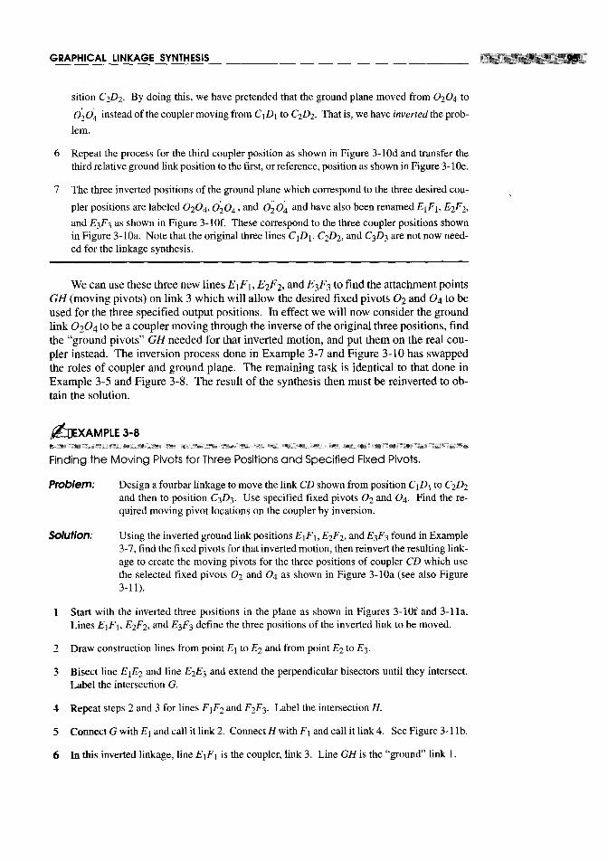
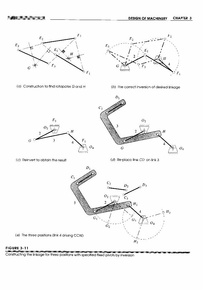

By inverting the original problem, we have reduced it to a more tractable form whichallows a direct solution by the general method of three-position synthesis from Exam-ples 3-5 and 3-6.
Position Synthesis for More Than Three Positions
It should be obvious that the more constraints we impose on these synthesis problems,the more complicated the task becomes to find a solution. When we define more thanthree positions of the output link, the difficulty increases substantially.
FOUR-POSITION SYNTHESIS does not lend itself as well to manual graphical so-lutions, though Hall [3] does present one approach. Probably the best approach is thatused by Sandor and Erdman [4] and others, which is a quantitative synthesis method andrequires a computer to execute it. Briefly, a set of simultaneous vector equations is writ-ten to represent the desired four positions of the entire linkage. These are then solvedafter some free choices of variable values are made by the designer. The computer pro-gram LINCAGES [1] by Erdman et aI., and the program KINSYN [5]by Kaufman, both pro-vide a convenient and user-friendly computer graphics based means to make the neces-sary design choices to solve the four-position problem. See Chapter 5 for further discussion.
3.5 QUICK-RETURN MECHANISMS
Many machine design applications have a need for a difference in average velocity be-tween their "forward" and "return" strokes. Typically some external work is being doneby the linkage on the forward stroke, and the return stroke needs to be accomplished as

rapidly as possible so that a maximum of time will be available for the working stroke.Many arrangements of links will provide this feature. The only problem is to synthesizethe right one!
Fourbar Quick-Return
The linkage synthesized in Example 3-1 is perhaps the simplest example of a fourbarlinkage design problem (see Figure 3-4, p. 84, and program FOURBAR disk fileF03-04.4br). It is a crank-rocker which gives two positions of the rocker with equal timefor the forward stroke and the return stroke. This is called a non-quick-retum linkage,and it is a special case of the more general quick-return case. The reason for its nonquick-return state is the positioning of the crank center 02 on the chord BIB2 extended.This results in equal angles of 180 degrees being swept out by the crank as it drives therocker from one extreme (toggle position) to the other. If the crank is rotating at con-stant angular velocity, as it will tend to when motor driven, then each 180 degree sweep,forward and back, will take the same time interval. Try this with your cardboard modelfrom Example 3-1 by rotating the crank at uniform velocity and observing the rockermotion and velocity.


This method works well for time ratios down to about 1:1.5. Beyond that value thetransmission angles become poor, and a more complex linkage is needed. Input the fileF03-12.4br to program FOURBARto see Example 3-9.
Sixbar Quick-Return
Larger time ratios, up to about 1:2, can be obtained by designing a sixbar linkage. Thestrategy here is to first design a fourbar drag link mechanism which has the desired timeratio between its driver crank and its driven or "dragged" crank, and then add a dyad(twobar) output stage, driven by the dragged crank. This dyad can be arranged to haveeither a rocker or a translating slider as the output link. First the drag link fourbar willbe synthesized; then the dyad will be added.

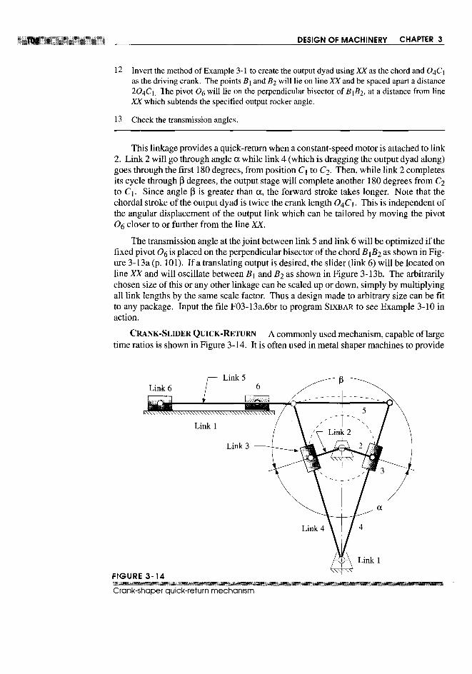

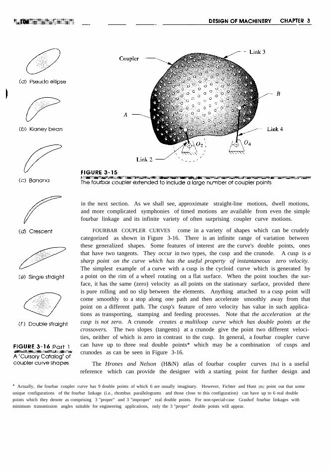
in the next section. As we shall see, approximate straight-line motions, dwell motions,and more complicated symphonies of timed motions are available from even the simplefourbar linkage and its infinite variety of often surprising coupler curve motions.
FOURBAR COUPLER CURVES come in a variety of shapes which can be crudelycategorized as shown in Figure 3-16. There is an infinite range of variation betweenthese generalized shapes. Some features of interest are the curve's double points, onesthat have two tangents. They occur in two types, the cusp and the crunode. A cusp is asharp point on the curve which has the useful property of instantaneous zero velocity.The simplest example of a curve with a cusp is the cycloid curve which is generated bya point on the rim of a wheel rotating on a flat surface. When the point touches the sur-face, it has the same (zero) velocity as all points on the stationary surface, provided thereis pure rolling and no slip between the elements. Anything attached to a cusp point willcome smoothly to a stop along one path and then accelerate smoothly away from thatpoint on a different path. The cusp's feature of zero velocity has value in such applica-tions as transporting, stamping and feeding processes. Note that the acceleration at thecusp is not zero. A crunode creates a multiloop curve which has double points at thecrossovers. The two slopes (tangents) at a crunode give the point two different veloci-ties, neither of which is zero in contrast to the cusp. In general, a fourbar coupler curvecan have up to three real double points* which may be a combination of cusps andcrunodes as can be seen in Figure 3-16.
The Hrones and Nelson (H&N) atlas of fourbar coupler curves [8a] is a usefulreference which can provide the designer with a starting point for further design and
* Actually, the fourbar coupler curve has 9 double points of which 6 are usually imaginary. However, Fichter and Hunt [8b] point out that someunique configurations of the fourbar linkage (i.e., rhombus parallelograms and those close to this configuration) can have up to 6 real doublepoints which they denote as comprising 3 "proper" and 3 "improper" real double points. For non-special-case Grashof fourbar linkages withminimum transmission angles suitable for engineering applications, only the 3 "proper" double points will appear.

analysis. It contains about 7000 coupler curves and defines the linkage geometry foreach of its Grashof crank-rocker linkages. Figure 3-17a reproduces a page from thisbook. The H&N atlas is logically arranged, with all linkages defined by their link ratios,based on a unit length crank. The coupler is shown as a matrix of fifty coupler points foreach linkage geometry, arranged ten to a page. Thus each linkage geometry occupies fivepages. Each page contains a schematic "key" in the upper right comer which defines thelink ratios.
Figure 3-l7b shows a "fleshed out" linkage drawn on top of the H&N atlas page toillustrate its relationship to the atlas information. The double circles in Figure 3-17 a de-fine the fixed pivots. The crank is always of unit length. The ratios of the other linklengths to the crank are given on each page. The actual link lengths can be scaled up ordown to suit your package constraints and this will affect the size but not the shape ofthe coupler curve. Anyone of the ten coupler points shown can be used by incorporat-ing it into a triangular coupler link. The location of the chosen coupler point can bescaled from the atlas and is defined within the coupler by the position vector R whoseconstant angle <I> is measured with respect to the line of centers of the coupler. The H&Ncoupler curves are shown as dashed lines. Each dash station represents five degrees ofcrank rotation. So, for an assumed constant crank velocity, the dash spacing is propor-tional to path velocity. The changes in velocity and the quick-return nature of the cou-pler path motion can be clearly seen from the dash spacing.
One can peruse this linkage atlas resource and find an approximate solution to vir-tually any path generation problem. Then one can take the tentative solution from theatlas to a CAE resource such as the FOURBARprogram or other package such as WorkingModel * and further refine the design, based on the complete analysis of positions, ve-locities, and accelerations provided by the program. The only data needed for the FOUR-BARprogram are the four link lengths and the location of the chosen coupler point withrespect to the line of centers of the coupler link as shown in Figure 3-17. These param-eters can be changed within program FOURBARto alter and refine the design. Input thefile F03-17bAbr to program FOURBARto animate the linkage shown in that figure.
An example of an application of a fourbar linkage to a practical problem is shownin Figure 3-18 which is a movie camera (or projector) film advance mechanism. Point02 is the crank pivot which is motor driven at constant speed. Point 04 is the rockerpivot, and points A and B are the moving pivots. Points A, B, and C define the couplerwhere C is the coupler point of interest. A movie is really a series of still pictures, each"frame" of which is projected for a small fraction of a second on the screen. Betweeneach picture, the film must be moved very quickly from one frame to the next while theshutter is closed to blank the screen. The whole cycle takes only 1/24 of a second. Thehuman eye's response time is too slow to notice the flicker associated with this discon-tinuous stream of still pictures, so it appears to us to be a continuum of changing images.
The linkage shown in Figure 3-18 is cleverly designed to provide the required mo-tion. A hook is cut into the coupler of this fourbar Grashof crank-rocker at point C whichgenerates the coupler curve shown. The hook will enter one of the sprocket holes in thefilm as it passes point Fl, Notice that the direction of motion of the hook at that point isnearly perpendicular to the film, so it enters the sprocket hole cleanly. It then turnsabruptly downward and follows a crudely approximate straight line as it rapidly pulls thefilm downward to the next frame. The film is separately guided in a straight track called

* The Hrones and Nelsonatlas is long out of print butmay be available fromUniversity Microfilms, AnnArbor, MI. Also, tbe Atlasof Linkage Design andAnalysis Vall: The Four BarLinkage similar to tbe H&Natlas, has been recentlypublished and is availablefrom Saltire Software, 9725SW Gemini Drive,Beaverton, OR 97005, (800)659-1874.

the "gate." The shutter (driven by another linkage from the same driveshaft at 02) isclosed during this interval of film motion, blanking the screen. At point F2 there is a cuspon the coupler curve which causes the hook to decelerate smoothly to zero velocity inthe vertical direction, and then as smoothly accelerate up and out of the sprocket hole.The abrupt transition of direction at the cusp allows the hook to back out of the holewithout jarring the film, which would make the image jump on the screen as the shutteropens. The rest of the coupler curve motion is essentially "wasting time" as it proceedsup the back side, to be ready to enter the film again to repeat the process. Input the fileF03-18.4br to program FOURBARto animate the linkage shown in that figure.
Some advantages of using this type of device for this application are that it is verysimple and inexpensive (only four links, one of which is the frame of the camera), isextremely reliable, has low friction if good bearings are used at the pivots, and can bereliably timed with the other events in the overall camera mechanism through commonshafting from a single motor. There are a myriad of other examples of fourbar couplercurves used in machines and mechanisms of all kinds.
One other example of a very different application is that of the automobile suspen-sion (Figure 3-19). Typically, the up and down motions of the car's wheels are controlledby some combination of planar fourbar linkages, arranged in duplicate to provide three-dimensional control as described in Section 3.2. Only a few manufacturers currently usea true spatial linkage in which the links are not arranged in parallel planes. In all casesthe wheel assembly is attached to the coupler of the linkage assembly, and its motion isalong a set of coupler curves. The orientation of the wheel is also of concern in this case,so this is not strictly a path generation problem. By designing the linkage to control thepaths of multiple points on the wheel (tire contact patch, wheel center, etc.-all of whichare points on the same coupler link extended), motion generation is achieved as the cou-pler has complex motion. Figure 3-19a and b shows parallel planar fourbar linkages sus-pending the wheels. The coupler curve of the wheel center is nearly a straight line overthe small vertical displacement required. This is desirable as the idea is to keep the tireperpendicular to the ground for best traction under all cornering and attitude changes ofthe car body. This is an application in which a non-Grashof linkage is perfectly accept-able, as full rotation of the wheel in this plane might have some undesirable results andsurprise the driver. Limit stops are of course provided to prevent such behavior, so evena Grashof linkage could be used. The springs support the weight of the vehicle and pro-vide a fifth, variable-length "force link" which stabilizes the mechanism as was describedin Section 2.14 (p. 54). The function of the fourbar linkage is solely to guide and controlthe wheel motions. Figure 3-19c shows a true spatial linkage of seven links (includingframe and wheel) and nine joints (some of which are ball-and-socket joints) used to con-trol the motion of the rear wheel. These links do not move in parallel planes but rathercontrol the three-dimensional motion of the coupler which carries the wheel assembly.
SYMMETRICAL FOURBAR COUPLER CURVES When a fourbar linkage's geome-try is such that the coupler and rocker are the same length pin-to-pin, all coupler pointsthat lie on a circle centered on the coupler-rocker joint with radius equal to the couplerlength will generate symmetrical coupler curves. Figure 3-20 shows such a linkage, itssymmetrical coupler curve, and the locus of all points that will give symmetrical curves.Using the notation of that figure, the criterion for coupler curve symmetry can be stated as:

* The nine independentparameters of a fourbarlinkage are: four linklengths, two coordinates ofthe coupler point withrespect to the coupler link,and three parameters thatdefine the location andorientation of the fixed linkin the global coordinatesystem.


This reference atlas is intended to be used as a starting point for a geared fivebarlinkage design. The link ratios, gear ratio, and phase angle can be input to the programFIVEBAR and then varied to observe the effects on coupler curve shape, velocities, andaccelerations. Asymmetry of links can be introduced, and a coupler point location otherthan the pin joint between links 3 and 4 defined within the FIVEBAR program as well.Note that program FIVEBAR expects the gear ratio to be in the form gear 2 / gear 5 whichis the inverse of the ratio A in the ZNH atlas.
3.7 COGNATES
It sometimes happens that a good solution to a linkage synthesis problem will be foundthat satisfies path generation constraints but which has the fixed pivots in inappropriatelocations for attachment to the available ground plane or frame. In such cases, the use ofa cognate to the linkage may be helpful. The term cognate was used by Hartenberg andDenavit [11] to describe a linkage, of different geometry, which generates the same cou-pler curve. Samuel Roberts (1875) and Chebyschev (1878) independently discoveredthe theorem which now bears their names:
Roberts-Chebyschev Theorem
Three different planar, pin-jointedfourbar linkages will trace identical coupler curves.
Hartenberg and Denavit[1I] presented extensions of this theorem to the slider-crank andthe sixbar linkages:

Two different planar slider-crank linkages will trace identical coupler curves.
The coupler-point curve of a planar fourbar linkage is also described by the joint of adyad of an appropriate sixbar linkage.
Figure 3-24a shows a fourbar linkage for which we want to find the two cognates.The first step is to release the fixed pivots DA and DB. While holding the coupler sta-tionary, rotate links 2 and 4 into colinearity with the line of centers (A IBI) of link 3 asshown in Figure 3-24b. We can now construct lines parallel to all sides of the links inthe original linkage to create the Cayley diagram in Figure 3-24c. This schematic ar-rangement defines the lengths and shapes oflinks 5 through 10 which belong to the cog-nates. All three fourbars share the original coupler point P and will thus generate thesame path motion on their coupler curves.
In order to find the correct location of the fixed pivot Dc from the Cayley diagram,the ends of links 2 and 4 are returned to the original locations of the fixed pivots DA andDB as shown in Figure 3-25a. The other links will follow this motion, maintaining theparallelogram relationships between links, and fixed pivot Dc will then be in its properlocation on the ground plane. This configuration is called a Roberts diagram-threefourbar linkage cognates which share the same coupler curve.
The Roberts diagram can be drawn directly from the original linkage without resortto the Cayley diagram by noting that the parallelograms which form the other cognatesare also present in the Roberts diagram and the three couplers are similar triangles. It isalso possible to locate fixed pivot Dc directly from the original linkage as shown in Fig-ure 3-25a. Construct a similar triangle to that of the coupler, placing its base (AB) be-tween DA and DB. Its vertex will be at Dc.
The ten-link Roberts configuration (Cayley's nine plus the ground) can now be ar-ticulated up to any toggle positions, and point P will describe the original coupler pathwhich is the same for all three cognates. Point Dc will not move when the Roberts link-age is articulated, proving that it is a ground pivot. The cognates can be separated asshown in Figure 3-25b and anyone of the three linkages used to generate the same cou-pler curve. Corresponding links in the cognates will have the same angular velocity asthe original mechanism as defined in Figure 3-25.
Nolle [12] reports on work by Luck [13] (in German) that defines the character of allfourbar cognates and their transmission angles. If the original linkage is a Grashof crank-rocker, then one cognate will be also, and the other will be a Grashof double rocker. Theminimum transmission angle of the crank-rocker cognate will be the same as that of theoriginal crank-rocker. If the original linkage is a Grashof double-crank (drag link), thenboth cognates will be also and their minimum transmission angles will be the same inpairs that are driven from the same fixed pivot. If the original linkage is a non-Grashoftriple-rocker, then both cognates are also triple-rockers.
These findings indicate that cognates of Grashof linkages do not offer improvedtransmission angles over the original linkage. Their main advantages are the differentfixed pivot location and different velocities and accelerations of other points in the link-age. While the coupler path is the same for all cognates, its velocities and accelerationswill not generally be the same since each cognate's overall geometry is different.
When the coupler point lies on the line of centers of link 3, the Cayley diagram de-generates to a group of colinear lines. A different approach is needed to determine the


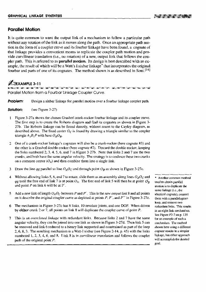


Program FOURBARcalculates the equivalent geared fivebar configuration for anyfourbar linkage and will export its data to a disk file that can be opened in program FIVE-BARfor analysis. The file F03-28aAbr can be opened in FOURBARto animate the link-age shown in Figure 3-28a. Then also open the file F03-28b.5br in program FIVEBARtosee the motion of the equivalent geared fivebar linkage. Note that the original fourbarlinkage is a triple-rocker, so cannot reach all portions of the coupler curve when drivenfrom one rocker. But, its geared fivebar equivalent linkage can make a full revolutionand traverses the entire coupler path. To export a FIVEBARdisk file for the equivalentGFBM of any fourbar linkage from program FOURBAR,use the Export selection underthe File pull-down menu.
3.8 STRAIGHT -LINE MECHANISMS
A very common application of coupler curves is the generation of approximate straightlines. Straight-line linkages have been known and used since the time of James Watt inthe 18th century. Many kinematicians such as Watt, Chebyschev, Peaucellier, Kempe,Evans, and Hoeken (as well as others) over a century ago, developed or discovered ei-ther approximate or exact straight-line linkages, and their names are associated withthose devices to this day.
The first recorded application of a coupler curve to a motion problem is that ofWatt's straight-line linkage, patented in 1784, and shown in Figure 3-29a. Watt de-vised his straight-line linkage to guide the long-stroke piston of his steam engine at a timewhen metal-cutting machinery that could create a long, straight guideway did not yetexist. * This triple-rocker linkage is still used in automobile suspension systems to guidethe rear axle up and down in a straight line as well as in many other applications.
Richard Roberts (1789-1864) (not to be confused with Samuel Roberts of the cog-nates) discovered the Roberts' straight-line linkage shown in Figure 3-29b. This is atriple-rocker. Chebyschev (1821-1894) also devised a straight-line linkage-a Grashofdouble-rocker-shown in Figure 3-29c.
The Hoeken linkage [16] in Figure 3-29d is a Grashof crank-rocker, which is a sig-nificant practical advantage. In addition, the Hoeken linkage has the feature of verynearly constant velocity along the center portion of its straight-line motion. It is inter-esting to note that the Hoecken and Chebyschev linkages are cognates of one another. tThe cognates shown in Figure 3-26 (p. 116) are the Chebyschev and Hoeken linkages.
These straight-line linkages are provided as built-in examples in program FOURBAR.A quick look in the Hrones and Nelson atlas of coupler curves will reveal a large numberof coupler curves with approximate straight-line segments. They are quite common.
To generate an exact straight line with only pin joints requires more than four links.At least six links and seven pin joints are needed to generate an exact straight line with apure revolute-jointed linkage, i.e., a Watt's or Stephenson's sixbar. A geared fivebarmechanism, with a gear ratio of -1 and a phase angle of 1t radians, will generate an exactstraight line at the joint between links 3 and 4. But this linkage is merely a transformedWatt's sixbar obtained by replacing one binary link with a higher joint in the form of agear pair. This geared fivebar's straight-line motion can be seen by reading the fileSTRAIGHT.5BRinto program FIVEBAR,calculating and animating the linkage.


Peaucellier * (1864) discovered an exact straight-line mechanism of eight bars andsix pins, shown in Figure 3-2ge. Links 5, 6, 7, 8 form a rhombus of convenient size.Links 3 and 4 can be any convenient but equal lengths. When OZ04 exactly equals OzA,point C generates an arc of infinite radius, i.e., an exact straight line. By moving thepivot Oz left or right from the position shown, changing only the length of link 1, thismechanism will generate true circle arcs with radii much larger than the link lengths.
Designing Optimum Straight-Line Fourbar Linkages
Given the fact that an exact straight line can be generated with six or more links usingonly revolute joints, why use a fourbar approximate straight-line linkage at all? Onereason is the desire for simplicity in machine design. The pin-jointed fourbar is the sim-plest possible one-DOF mechanism. Another reason is that a very good approximationto a true straight line can be obtained with just four links, and this is often "good enough"for the needs of the machine being designed. Manufacturing tolerances will, after all,cause any mechanism's performance to be less than ideal. As the number of links andjoints increases, the probability that an exact-straight-line mechanism will deliver its the-oretical performance in practice is obviously reduced.
* Peaucellier was a Frencharmy captain and military There is a real need for straight-line motions in machinery of all kinds, especially inengineer who first proposed automated production machinery. Many consumer products such as cameras, film, toi-his "compas compose" or letries, razors, and bottles are manufactured, decorated, or assembled on sophisticatedcompound compass in 1864 and complicated machines that contain a myriad of linkages and cam-follower systems.but received no immediate Traditionally, most of this kind of production equipment has been of the intermittent-recognition therefor. The motion variety. This means that the product is carried through the machine on a linear orBritish-Americanmathematician, James rotary conveyor that stops for any operation to be done on the product, and then indexesSylvester, reported on it to the product to the next work station where it again stops for another operation to be per-the Atheneum Club in formed. The forces and power required to accelerate and decelerate the large mass ofLondon in 1874. He the conveyor (which is independent of, and typically larger than, the mass of the prod-observed that "The perfect uct) severely limit the speeds at which these machines can be run.parallel motion ofPeaucellier looks so simple Economic considerations continually demand higher production rates, requiringand moves so easily that higher speeds or additional, expensive machines. This economic pressure has causedpeople who see it at work many manufacturers to redesign their assembly equipment for continuous conveyoralmost universally express motion. When the product is in continuous motion in a straight line and at constant ve-astonishment that it waitedso long to be discovered." A locity, every workhead that operates on the product must be articulated to chase the prod-model of the Peaucellier uct and match both its straight-line path and its constant velocity while performing thelinkage was passed around task. These factors have increased the need for straight-line mechanisms, including onesthe table. The famous capable of near-constant velocity over the straight-line path.physicist, Sir William
A (near) perfect straight-line motion is easily obtained with a fourbar slider-crankThomson (later LordKelvin), refused to mechanism. Ball-bushings (Figure 2-26, p. 57) and hardened ways are available com-relinquish it, declaring "No. mercially at moderate cost and make this a reasonable, low-friction solution to theI have not had nearly straight-line path guidance problem. But, the cost and lubrication problems of a proper-enough of it-it is the most ly guided slider-crank mechanism are still greater than those of a pin-jointed fourbar link-beautiful thing I have ever age. Moreover, a crank-slider-block has a velocity profile that is nearly sinusoidal (withseen in my life." Source:Strandh, S. (1979). A some harmonic content) and is far from having constant velocity over any of its motion.History of the Machine. The Hoeken-type linkage offers an 0l?timum combination of straightness and nearA&W Publishers: NewYork, p. 67. constant velocity and is a crank-rocker, so it can be motor driven. Its geometry, dimen-

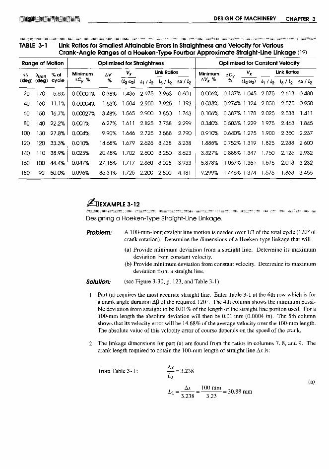

3.9 DWELL MECHANISMS
A common requirement in machine design problems is the need for a dwell in the outputmotion. A dwell is defined as zero output motionfor some nonzero input motion. In otherwords, the motor keeps going, but the output link stops moving. Many production ma-chines perform a series of operations which involve feeding a part or tool into a work-space, and then holding it there (in a dwell) while some task is performed. Then the partmust be removed from the workspace, and perhaps held in a second dwell while the restof the machine "catches up" by indexing or performing some other tasks. Cams andfollowers (Chapter 8) are often used for these tasks because it is trivially easy to create a

dwell with a earn. But, there is always a trade-off in engineering design, and cams havetheir problems of high cost and wear as described in Section 2.15 (p. 55).
It is also possible to obtain dwells with "pure" linkages of only links and pin joints,which have the advantage over cams of low cost and high reliability. Dwell linkages aremore difficult to design than are cams with dwells. Linkages will usually yield only anapproximate dwell but will be much cheaper to make and maintain than cams. Thus theymay be well worth the effort.
Single-Dwell Linkages
There are two usual approaches to designing single-dwell linkages. Both result in six-bar mechanisms, and both require first finding a fourbar with a suitable coupler curve.A dyad is then added to provide an output link with the desired dwell characteristic. Thefirst approach to be discussed requires the design or definition of a fourbar with a cou-pler curve that contains an approximate circle arc portion, which "are" occupies the de-sired portion of the input link (crank) cycle designated as the dwell. An atlas of couplercurves is invaluable for this part of the task. Symmetrical coupler curves are also wellsuited to this task, and the information in Figure 3-21 (p. 110) can be used to find them.
Problem: Design a sixbar linkage for 90° rocker motion over 300 crank degrees with dwellfor the remaining 60°.
Solution: (see Figure 3-31)
I Search the H&N atlas for a fourbar linkage with a coupler curve having an approximate(pseudo) circle arc portion which occupies 60° of crank motion (12 dashes). The chosen four-bar is shown in Figure 3-3Ia.
2 Layout this linkage to scale including the coupler curve and find the approximate center ofthe chosen coupler curve pseudo-arc using graphical geometric techniques. To do so, drawthe chord of the arc and construct its perpendicular bisector as shown in Figure 3-31b. Thecenter will lie on the bisector. Label this point D.
3 Set your compass to the approximate radius of the coupler arc. This will be the length oflink 5 which is to be attached at the coupler point P.
4 Trace the coupler curve with the compass point, while keeping the compass pencil lead onthe perpendicular bisector, and find the extreme location along the bisector that the compasslead will reach. Label this point E.
5 The line segment DE represents the maximum displacement that a link of length CD, at-tached at P, will reach along the bisector.
6 Construct a perpendicular bisector of the line segment DE, and extend it in a convenient di-rection.


This linkage dwells because, during the time that the coupler point P is traversingthe pseudo-arc portion of the coupler curve, the other end of link 5, attached to P and thesame length as the arc radius, is essentially stationary at its other end, which is the arccenter. However the dwell at point D will have some "jitter" or oscillation, due to thefact that D is only an approximate center of the pseudo-arc on the sixth-degree couplercurve. When point P leaves the arc portion, it will smoothly drive link 5 from point D topoint E, which will in turn rotate the output link 6 through its arc as shown in Figure3-31c (p. 127). Note that we can have any angular displacement of link 6 we desire withthe same links 2 to 5, as they alone completely define the dwell aspect. Moving pivot06 left and right along the bisector of line DE will change the angular displacement oflink 6 but not its timing. In fact, a slider block could be substituted for link 6 as shownin Figure 3-31d, and linear translation along line DE with the same timing and dwell atD will result. Input the file F03-31c.6br to program SIXBARand animate to see the link-age of Example 3-13 in motion. The dwell in the motion of link 6 can be clearly seen inthe animation, including the jitter due to its approximate nature.
Double-Dwell Linkages
It is also possible, using a fourbar coupler curve, to create a double-dwell output motion.One approach is the same as that used in the single-dwell of Example 3-11. Now a cou-pler curve is needed which has two approximate circle arcs of the same radius but withdifferent centers, both convex or both concave. A link 5 of length equal to the radius ofthe two arcs will be added such that it and link 6 will remain nearly stationary at the cen-ter of each of the arcs, while the coupler point traverses the circular parts of its path. Mo-tion of the output link 6 will occur only when the coupler point is between those arc por-tions. Higher-order linkages, such as the geared fivebar, can be used to create multiple-dwell outputs by a similar technique since they possess coupler curves with multiple, ap-proximate circle arcs. See the built-in example double-dwell linkage in program SIXBARfor a demonstration of this approach.
A second approach uses a coupler curve with two approximate straight-line seg-ments of appropriate duration. If a pivoted slider block (link 5) is attached to the cou-pler at this point, and link 6 is allowed to slide in link 5, it only remains to choose a pivot06 at the intersection of the straight-line segments extended. The result is shown in Fig-ure 3-32. While block 5 is traversing the "straight-line" segments of the curve, it willnot impart any angular motion to link 6. The approximate nature of the fourbar straightline causes some jitter in these dwells also.


7a Kempe,A. B. (1876). "On a General Method of Describing Plane Curves of the Nth Degree byLinkwork." Proceedings London Mathematical Society, 7, pp. 213-216.
7b Wunderlich, W. (1963). "Hahere Koppelkurven." Osterreichisches Ingenieur Archiv, XVll(3), pp.162-165.
8a Hrones, J. A., and G. L. Nelson. (1951). Analysis of the Fourbar Linkage. MIT Technology Press:Cambridge, MA.
8b Fichter, E. F., and K. H. Hunt. (1979). 'The Variety, Cognate Relationships, Class, and Degenera-tion of the Coupler Curves of the Planar 4R Linkage." Proc. of 5th World Congress on Theory ofMachines and Mechanisms, Montreal, pp. 1028-1031.
9 Kota, S. (1992). "Automatic Selection of Mechanism Designs from a Three-Dimensional DesignMap." Journal of Mechanical Design, 114(3), pp. 359-367.
10 Zhang, c., R. L. Norton, and T. Hammond. (1984). "Optimization of Parameters for SpecifiedPath Generation Using an Atlas of Coupler Curves of Geared Five-Bar Linkages." Mechanism andMachine Theory, 19(6), pp. 459-466.
11 Hartenberg, R. S., and J. Denavit. (1959). "Cognate Linkages." Machine Design, April 16, 1959,pp.149-152.
12 Nolle, H. (1974). "Linkage Coupler Curve Synthesis: A Historical Review - II. Developments after1875." Mechanism and Machine Theory, 9,1974, pp. 325-348.
13 Luck, K. (1959). "Zur Erzeugung von Koppelkurven viergliedriger Getriebe." Maschinenbautech-nik (Getriebetechnik), 8(2), pp. 97-104.
14 Soni,A. H. (1974). Mechanism Synthesis and Analysis. Scripta, McGraw-Hili: New York, pp. 381-382.
15 Hall, A. S. (1961). Kinematics and Linkage Design. Waveland Press: Prospect Heights, IL, p. 51.
16 Hoeken, K. (1926). "Steigerung der Wirtschaftlichkeit durch zweckmaBige." Anwendung derGetriebelehre Werkstattstechnik.
17 Hain, K. (1967). Applied Kinematics. D. P. Adams, translator. McGraw-Hili: New York, pp. 308-309.
18 Nolle, H. (1974). "Linkage Coupler Curve Synthesis: A Historical Review -I. Developments up to1875." Mechanism and Machine Theory, 9, pp.147-l68.
19 Norton, R. L. (1998). "In Search of the "Perfect" Straight Line and Constant Velocity Too."Submitted to the ASME Journal of Mechanical Design.
For additional information on type synthesis, the following are recommended:
Artoholevsky, I. I. (1975). Mechanisms in Modern Engineering Design. N. Weinstein, translator. Vol. I to Iv. MIRPublishers: Moscow.
Chironis, N. P., ed. (1965). Mechanisms, Linkages, and Mechanical Controls. McGraw-Hill: New York.
Chironis, N. P., ed. (1966). Machine Devices and Instrumentation. McGraw-Hill: New York.
Jensen, P. W. (1991). Classical and Modern Mechanisms for Engineers and Inventors. Marcel Dekker: New York.
Jones, F., H. Horton, and J. Newell. (1967). Ingenious Mechanisms for Engineers. Vol. I to N. Industrial Press: NewYork.
Olson, D. G., et a1. (1985). "A Systematic Procedure for Type Synthesis of Mechanisms with Literature Review."Mechanism and Machine Theory, 20(4), pp. 285-295.
Thttle, S. B. (1967). Mechanisms for Engineering Design. John Wiley & Sons: New York.


3-4 Design a fourbar mechanism to give the two positions shown in Figure P3-1 of couplermotion. (See Example 3-3.) Build a cardboard model and determine the toggle positionsand the minimum transmission angle. Add a driver dyad. (See Example 3-4.)
*3-5 Design a fourbar mechanism to give the three positions of coupler motion with no quick-return shown in Figure P3-2. (See also Example 3-5.) Ignore the points OA and OBshown. Build a cardboard model and determine the toggle positions and the minimumtransmission angle. Add a driver dyad. (See Example 3-4.)
*3-6 Design a fourbar mechanism to give the three positions shown in Figure P3-2 using thefixed pivots OA and OB shown. Build a cardboard model and determine the togglepositions and the minimum transmission angle. Add a driver dyad.
3-7 Repeat Problem 3-2 with a quick-return time ratio of 1:1.4. (See Example 3-9.)
*3-8 Design a sixbar drag link quick-return linkage for a time ratio of 1:2, and output rockermotion of 60°.
3-9 Design a crank shaper quick-return mechanism for a time ratio of 1 : 3 (Figure 3-14, p.102).
*3-10 Find the two cognates of the linkage in Figure 3-17 (p. 106). Draw the Cayley andRoberts diagrams. Check your results with program FOURBAR.


*3-42 Find the Grashof condition, any limit positions, and the extreme values of the transmis-sion angle (to graphical accuracy) of the linkage in Figure P3-l2.
3-43 Draw the Roberts diagram and find the cognates of the linkage in Figure P3-l2.
3-44 Find the three geared fivebar cognates of the linkage in Figure P3-l2.
3-45 Prove that the relationships between the angular velocities of various links in the Robertsdiagram as shown in Figure 3-25 (p. 115) are true.
3-46 Design a fourbar linkage to move the object in Figure P3-l3 from position 1 to 2 usingpoints A and B for attachment. Add a driver dyad to limit its motion to the range ofpositions shown making it a sixbar. All fixed pivots should be on the base.
3-47 Design a fourbar linkage to move the object in Figure P3-13 from position 2 to 3 usingpoints A and B for attachment. Add a driver dyad to limit its motion to the range ofpositions shown making it a sixbar. All fixed pivots should be on the base.
3-48 Design a fourbar linkage to move the object in Figure P3-l3 through the three positionsshown using points A and B for attachment. Add a driver dyad to limit its motion to therange of positions shown making it a sixbar. All fixed pivots should be on the base.
3-49 Design a fourbar linkage to move the object in Figure P3-l4 from position 1 to 2 usingpoints A and B for attachment. Add a driver dyad to limit its motion to the range ofpositions shown making it a sixbar. All fixed pivots should be on the base.
3-50 Design a fourbar linkage to move the object in Figure P3-l4 from position 2 to 3 usingpoints A and B for attachment. Add a driver dyad to limit its motion to the range ofpositions shown making it a sixbar. All fixed pivots should be on the base.
3-51 Design a fourbar linkage to move the object in Figure P3-l4 through the three positionsshown using points A and B for attachment. Add a driver dyad to limit its motion to therange of positions shown making it a sixbar. All fixed pivots should be on the base.
3-52 Design a fourbar linkage to move the object in Figure P3-l5 from position 1 to 2 usingpoints A and B for attachment. Add a driver dyad to limit its motion to the range ofpositions shown making it a sixbar. All fixed pivots should be on the base.


must be random. The device should operate automatically and unattended except for therefill of balls. It should be capable of firing 50 balls between reloads. The timing of ballreleases should vary. For simplicity, a motor driven pin-jointed linkage design ispreferred.
P3-2 A quadriplegic patient has lost all motion except that of her head. She can only move asmall "mouth stick" to effect a switch closure. She was an avid reader before her injuryand would like again to be able to read standard hardcover books without the need of aperson to turn pages for her. Thus, a reliable, simple, and inexpensive automatic pagetumer is needed. The book may be placed in the device by an assistant. It shouldaccommodate as wide a range of book sizes as possible. Book damage is to be avoidedand safety of the user is paramount.
P3-3 Grandma's off her rocker again! Junior's run down to the Bingo parlor to fetch her, butwe've got to do something about her rocking chair before she gets back. She's beencomplaining that her arthritis makes it too painful to push the rocker. So, for her l00thbirthday in 2 weeks, we're going to surprise her with a new, automated, motorized rockingchair. The only constraints placed on the problem are that the device must be safe andmust provide interesting and pleasant motions, similar to those of her present Bostonrocker, to all parts of the occupant's body. Since simplicity is the mark of good design, alinkage solution with only full pin joints is preferred.
P3-4 The local amusement park's business is suffering as a result of the proliferation ofcomputer game parlors. They need a new and more exciting ride which will attract newcustomers. The only constraints are that it must be safe, provide excitement, and notsubject the occupants to excessive accelerations or velocities. Also it must be as compactas possible, since space is limited. Continuous rotary input and full pin joints arepreferred.
P3-5 The student section of ASME is sponsoring a spring fling on campus. They need amechanism for their "Dunk the Professor" booth which will carry the unfortunate(untenured) volunteer into and out of the water tub. The contestants will provide theinputs to a multiple-DOF mechanism. If they know their kinematics, they can provide acombination of inputs which will dunk the victim.
P3-6 The National House of Flapjacks wants to automate their flapjack production. They needa mechanism which will automatically flip the flapjacks "on the fly" as they travelthrough the griddle on a continuously moving conveyor. This mechanism must track theconstant velocity of the conveyor, pick up a pancake, flip it over and place it back onto theconveyor.
P3-7 Many varieties and shapes of computer video monitors now exist. Their long-term useleads to eyestrain and body fatigue. There is a need for an adjustable stand which willhold the video monitor and the separate keyboard at any position the user deemscomfortable. The computer's central processor unit (CPU) can be remotely located. Thisdevice should be freestanding to allow use with a comfortable chair, couch, or lounge ofthe user's choice. It should not require the user to assume the conventional "seated at adesk" posture to use the computer. It must be stable in all positions and safely support theequipment's weight.
P3-8 Most small boat trailers must be submerged in the water to launch or retrieve the boat.This greatly reduces the life of the trailer, especially in salt water. A need exists for atrailer that will remain on dry land while it launches or retrieves the boat. No part of thetrailer should get wet. User safety is of greatest concern, as is protection of the boat fromdamage.

P3-9 The "Save the Skeet" foundation has requested a more humane skeet launcher bedesigned. While they have not yet succeeded in passing legislation to prevent thewholesale slaughter of these little devils, they are concerned about the inhumane aspectsof the large accelerations imparted to the skeet as it is launched into the sky for thesportsman to shoot it down. The need is for a skeet launcher that will smoothly acceleratethe clay pigeon onto its desired trajectory.
P3-10 The coin operated "kid bouncer" machines found outside supermarkets typically provide avery unimaginative rocking motion to the occupant. There is a need for a superior"bouncer" which will give more interesting motions while remaining safe for smallchildren.
P3-11 Horseback riding is a very expensive hobby or sport. There is a need for a horsebackriding simulator to train prospective riders sans the expensive horse. This device shouldprovide similar motions to the occupant as she would feel in the saddle under various gaitssuch as a walk, canter, or gallop. A more advanced version might contain jumpingmotions as well. User safety is most important.
P3-12 The nation is on a fitness craze. Many exercise machines have been devised. There isstill room for improvement to these devices. They are typically designed for the young,strong athlete. There is also a need for an ergonomically optimum exercise machine forthe older person who needs gentler exercise.
P3-13 A paraplegic patient needs a device to get himself from his wheelchair into the Jacuzziwith no assistance. He has good upper body and arm strength. Safety is paramount.
P3-14 The army has requested a mechanical walking device to test army boots for durability. Itshould mimic a person's walking motion and provide forces similar to an averagesoldier's foot.
P3-15 NASA wants a zero-G machine for astronaut training. It must carry one person andprovide a negative I-G acceleration for as long as possible.
P3-16 The Amusement Machine Co. Inc. wants a portable "whip" ride which will give two orfour passengers a thrilling but safe ride, and which can be trailed behind a pickup truckfrom one location to another.
P3-17 The Air Force has requested a pilot training simulator which will give potential pilotsexposure to G forces similar to those they will experience in dogfight maneuvers.
P3-18 Cheers needs a better "mechanical bull" simulator for their "yuppie" bar in Boston. Itmust give a thrilling "bucking bronco" ride but be safe.
P3-19 Despite the improvements in handicap access, many curbs block wheelchairs from publicplaces. Design an attachment for a conventional wheelchair which will allow it to get upover a curb.
P3-20 A carpenter needs a dumping attachment to fit in her pickup truck so she can dumpbuilding materials. She can't afford to buy a dump truck.
P3-21 The carpenter in Project P3-20 wants an inexpensive lift gate designed to fit her full-sizedpickup truck, in order to lift and lower heavy cargo to the truck bed.
P3-22 The carpenter in Project P3-20 is very demanding (and lazy). She also wants a device tolift Sheet rock into place on ceilings or walls to hold it while she nails it on.

P3-23 Click and Clack, the tappet brothers, need a better transmission jack for their Good NewsGarage. This device should position a transmission under a car (on a lift) and allow it tobe maneuvered into place safely and quickly.
P3-24 A paraplegic who was an avid golfer before his injury, wants a mechanism to allow him tostand up in his wheelchair in order to once again play golf. It must not interfere withnormal wheelchair use, though it could be removed from the chair when he is not golfing.
P3-25 A wheelchair lift is needed to raise the wheelchair and person 3 ft from the garage floor tothe level of the first floor of the house. Safety and reliability are of major concern, as iscost.
P3-26 A paraplegic needs a mechanism that can be installed on a full-size 3-door pickup truckthat will lift the wheelchair into the area behind the driver's seat. This person hasexcellent upper body strength and, with the aid of specially installed handles on the truck,can get into the cab from the chair. The truck can be modified as necessary to accommo-date this task. For example, attachment points can be added to its structure and the backseat of the truck can be removed if necessary.
P3-27 There is demand for a better Baby Transport Device. Many such devices are on themarket. Some are called carriages, some strollers. Some are convertible to multiple uses.Our marketing survey data so far seems to indicate that the customers want portability(i.e., foldability), light weight, one-handed operation, and large wheels. Some of thesefeatures are present in existing devices. We need a better design that more completelymeets the needs of the customer. The device must be stable, effective, and safe for thebaby and the operator. Full joints are preferred to half joints and simplicity is the mark ofgood design. A linkage solution with manual input is desired.
P3-28 There is a need for a dining-table leaf insertion device. The device must be simple to use,preferably using the action of opening the table-halves as the actuating motion. That is, asyou pull the table open, the stored leaf should be carried by the mechanism of your designinto its proper place in order to extend the dining surface.
P3-29 A boat owner has requested that we design her a lift mechanism to automatically move alOOO-lb,15-ft boat from a cradle on land to the water. A seawall protects the owner'syard, and the boat cradle sits above the seawall. The tidal variation is 4 ft. Your mecha-nism will be attached to land and move the boat from its stored position on the cradle tothe water and return it to the cradle. The device must be safe and easy to use and notoverly expensive.
P3-30 The landfills are full! We're about to be up to our ears in trash! The world needs a bettertrash compactor. It should be simple, inexpensive, quiet, compact, and safe. It can eitherbe manually powered or motorized, but manual operation is preferred to keep the costdown. The device must be stable, effective, and safe for the operator.
P3-31 A small contractor needs a mini-dumpster attachment for his pickup truck. He has madeseveral trash containers which are 4 ft X 4 ft X 3.5 ft high. The empty container weighsISO lb. He needs a mechanism which he can attach to his fleet of standard, full-sizepickup trucks (Chevrolet, Ford, or Dodge). This mechanism should be able to pick up thefull trash container from the ground, lift it over the closed tailgate of the truck, dump itscontents into the truck bed, and then return it empty to the ground. He would like not totip his truck over in the process. The mechanism should store permanently on the truck insuch a manner as to allow the normal use of the pickup truck at all other times. You mayspecify any means of attachment of your mechanism to the container and to the truck.

Once a tentative mechanism design has been synthesized, it must then be analyzed. Aprincipal goal of kinematic analysis is to determine the accelerations of all the movingparts in the assembly. Dynamic forces are proportional to acceleration, from Newton'ssecond law. We need to know the dynamic forces in order to calculate the stresses in thecomponents. The design engineer must ensure that the proposed mechanism or machinewill not fail under its operating conditions. Thus the stresses in the materials must be keptwell below allowable levels. To calculate the stresses, we need to know the static anddynamic forces on the parts. To calculate the dynamic forces, we need to know the ac-celerations. In order to calculate the accelerations, we must first find the positions ofall the links or elements in the mechanism for each increment of input motion, and thendifferentiate the position equations versus time to find velocities, and then differentiateagain to obtain the expressions for acceleration. For example, in a simple Grashof four-bar linkage, we would probably want to calculate the positions, velocities, and accelera-tions of the output links (coupler and rocker) for perhaps every two degrees (180 posi-tions) of input crank position for one revolution of the crank.
This can be done by any of several methods. We could use a graphical approachto determine the position, velocity, and acceleration ofthe output links for all 180 posi-tions of interest, or we could derive the general equations of motion for any position,differentiate for velocity and acceleration, and then solve these analytical expressionsfor our 180 (or more) crank locations. A computer will make this latter task much morepalatable. If we choose to use the graphical approach to analysis, we will have to do anindependent graphical solution for each of the positions of interest. None of the infor-mation obtained graphically for the first position will be applicable to the second posi-tion or to any others. In contrast, once the analytical solution is derived for a particular

mechanism, it can be quickly solved (with a computer) for all positions. If you wantinformation for more than 180 positions, it only means you will have to wait longer forthe computer to generate those data. The derived equations are the same. So, have an-other cup of coffee while the computer crunches the numbers! In this chapter, we willpresent and derive analytical solutions to the position analysis problem for various pla-nar mechanisms. We will also discuss graphical solutions which are useful for checkingyour analytical results. In Chapters 6 and 7 we will do the same for velocity and accel-eration analysis of planar mechanisms.
It is interesting to note that graphical position analysis of linkages is a truly trivialexercise, while the algebraic approach to position analysis is much more complicated.If you can draw the linkage to scale, you have then solved the position analysis problemgraphically. It only remains to measure the link angles on the scale drawing to protrac-tor accuracy. But, the converse is true for velocity and especially for acceleration anal-ysis. Analytical solutions for these are less complicated to derive than is the analyticalposition solution. However, graphical velocity and acceleration analysis becomes quitecomplex and difficult. Moreover, the graphical vector diagrams must be redone de novo(meaning literally from new) for each of the linkage positions of interest. This is a verytedious exercise and was the only practical method available in the days B.c. (BeforeComputer), not so long ago. The proliferation of inexpensive microcomputers in recentyears has truly revolutionized the practice of engineering. As a graduate engineer, youwill never be far from a computer of sufficient power to solve this type of problem andmay even have one in your pocket. Thus, in this text we will emphasize analytical solu-tions which are easily solved with a microcomputer. The computer programs providedwith this text use the same analytical techniques as derived in the text.
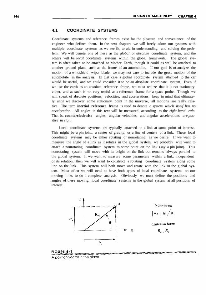
4.1 COORDINATE SYSTEMS
Coordinate systems and reference frames exist for the pleasure and convenience of theengineer who defines them. In the next chapters we will freely adorn our systems withmultiple coordinate systems as we see fit, to aid in understanding and solving the prob-lem. We will denote one of these as the global or absolute coordinate system, and theothers will be local coordinate systems within the global framework. The global sys-tem is often taken to be attached to Mother Earth, though it could as well be attached toanother ground plane such as the frame of an automobile. If our goal is to analyze themotion of a windshield wiper blade, we may not care to include the gross motion of theautomobile in the analysis. In that case a global coordinate system attached to the carwould be useful, and we could consider it to be an absolute coordinate system. Even ifwe use the earth as an absolute reference frame, we must realize that it is not stationaryeither, and as such is not very useful as a reference frame for a space probe. Though wewill speak of absolute positions, velocities, and accelerations, keep in mind that ultimate-ly, until we discover some stationary point in the universe, all motions are really rela-tive. The term inertial reference frame is used to denote a system which itself has noacceleration. All angles in this text will be measured according to the right-hand rule.That is, counterclockwise angles, angular velocities, and angular accelerations are pos-itive in sign.
Local coordinate systems are typically attached to a link at some point of interest.This might be a pin joint, a center of gravity, or a line of centers of a link. These localcoordinate systems may be either rotating or nonrotating as we desire. If we want tomeasure the angle of a link as it rotates in the global system, we probably will want toattach a nonrotating coordinate system to some point on the link (say a pin joint). Thisnonrotating system will move with its origin on the link but remains always parallel tothe global system. If we want to measure some parameters within a link, independentof its rotation, then we will want to construct a rotating coordinate system along someline on the link. This system will both move and rotate with the link in the global sys-tem. Most often we will need to have both types of local coordinate systems on ourmoving links to do a complete analysis. Obviously we must define the positions andangles of these moving, local coordinate systems in the global system at all positions ofinterest.

DisplacementDisplacement of a point is the change in its position and can be defined as the straight-line distance between the initial and final position of a point which has moved in the ref-erence frame. Note that displacement is not necessarily the same as the path lengthwhich the point may have traveled to get from its initial to final position. Figure 4-2ashows a point in two positions, A and B. The curved line depicts the path along whichthe point traveled. The position vector RBA defines the displacement of the point B withrespect to pointA. Figure 4-2b defines this situation more rigorously and with respect toa reference frame XY. The notation R will be used to denote a position vector. The vec-tors RA and RB define, respectively, the absolute positions of points A and B with respectto this global XY reference frame. The vector RBA denotes the difference in position, orthe displacement, between A and B. This can be expressed as the position differenceequation:
RBA=RB-RA (4.1a)
This expression is read: The position of B with respect to A is equal to the (absolute)position of B minus the (absolute) position of A, where absolute means with respect tothe origin of the global reference frame. This expression could also be written as:
RBA =RBO-RAO (4.1b)
with the second subscript 0 denoting the origin of the XY reference frame. When a posi-tion vector is rooted at the origin of the reference frame, it is customary to omit the sec-ond subscript. It is understood, in its absence, to be the origin. Also, a vector referred tothe origin, such as RA, is often called an absolute vector. This means that it is taken withrespect to a reference frame which is assumed to be stationary, e.g. the ground. It isimportant to realize, however, that the ground is usually also in motion in some largerframe ofreference. Figure 4-2c shows a graphical solution to equation 4.1.

In our example of Figure 4-2, we have tacitly assumed so far that this point, whichis first located at A and later at B, is, in fact, the same particle, moving within the refer-ence frame. It could be, for example, one automobile moving along the road from A to B.With that assumption, it is conventional to refer to the vector RBA as a position differ-ence. There is, however, another situation which leads to the same diagram and equa-tion but needs a different name. Assume now that points A and B in Figure 4-2b repre-sent not the same particle but two independent particles moving in the same referenceframe, as perhaps two automobiles traveling on the same road. The vector equations 4.1and the diagram in Figure 4-2b still are valid, but we now refer to RBA as a relative po-sition, or apparent position. We will use the relative position term here. A more for-mal way to distinguish between these two cases is as follows:
CASE 1: One body in two successive positions =>position difference
CASE 2: Two bodies simultaneously in separate positions => relative position
This may seem a rather fine point to distinguish, but the distinction will prove use-ful, and the reasons for it more clear, when we analyze velocities and accelerations, es-pecially when we encounter (CASE 2 type) situations in which the two bodies occupy thesame position at the same time but have different motions.


A two-argument arctangent function must be used to solve equations 4.2g since the an-gles can be in any quadrant. Equations 4.2 can be encoded in any computer language orequation solver, and the value of 82 varied over the linkage's usable range to find all cor-responding values of the other two link angles.
Vector Loop Representation of linkages
An alternate approach to linkage position analysis creates a vector loop (or loops) aroundthe linkage. This approach offers some advantages in the synthesis of linkages whichwill be addressed in Chapter 5. The links are represented as position vectors. Figure4-6 shows the same fourbar linkage as in Figure 4-4 (p. 151) , but the links are now drawnas position vectors which form a vector loop. This loop closes on itself making the sumof the vectors around the loop zero. The lengths of the vectors are the link lengths which

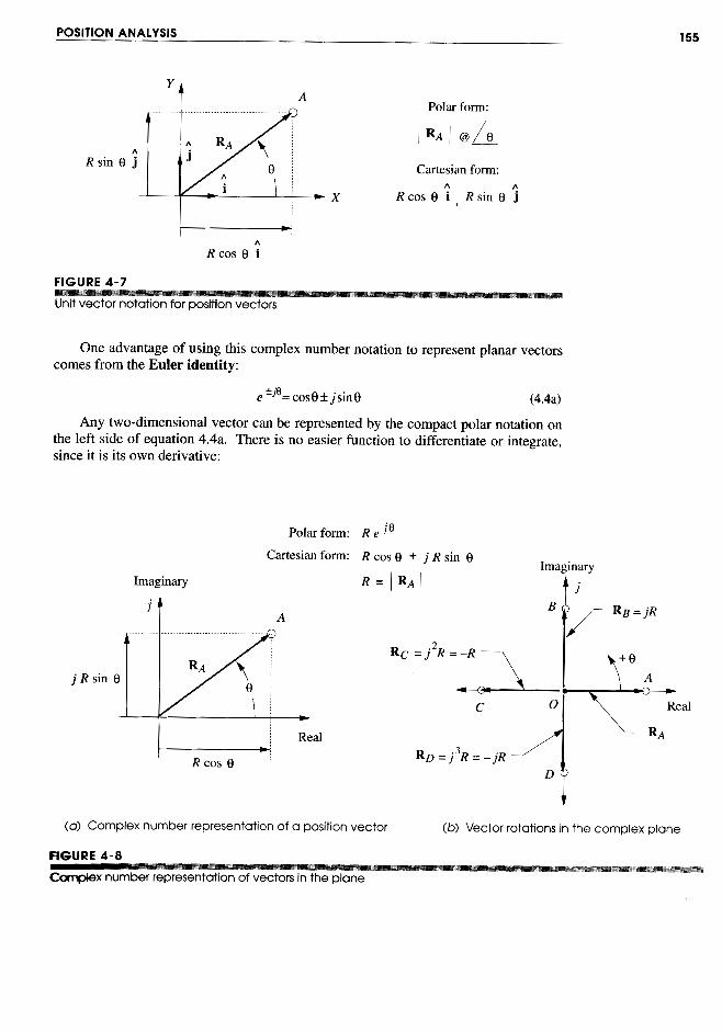


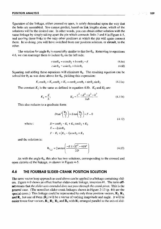


4.7 AN INVERTED SLIDER-CRANK POSITION SOLUTION
Figure 4-l0a shows inversion #3 of the common fourbar slider-crank linkage in whichthe sliding joint is between links 3 and 4 at point B. This is shown as an offset slider-crank mechanism. The slider block has pure rotation with its center offset from the slideaxis. (Figure 2-l3c, p. 44, shows the nonoffset version of this linkage in which the vec-tor R.t is zero.)
The global coordinate system is again taken with its origin at input crank pivot 02and the positive X axis along link 1, the ground link. A local axis system has been placedat point B in order to define 83. Note that there is a fixed angle 'Ywithin link 4 whichdefines the slot angle with respect to that link.
In Figure 4-l0b the links have been represented as position vectors having sensesconsistent with the coordinate systems that were chosen for convenience in defining the


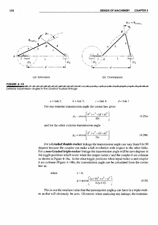


Only one of these ± cases will produce an argument for the arccosine function whichlies between ±1. The toggle angle which is in the first or second quadrant can be foundfrom this value. The other toggle angle will then be the negative of the one found, due tothe mirror symmetry of the two toggle positions about the ground link as shown in Fig-ure 4-16 (p. 171). Program FOURBARcomputes the values of these toggle angles for anynon-Grashof linkage.

4.12 CIRCUITS AND BRANCHES IN LINKAGES
In Section 4.5 it was noted that the fourbar linkage position problem has two solutionswhich correspond to the two circuits of the linkage. This section will explore the topicsof circuits and branches in linkages in more detail.
Chase and Mirth[2] define a circuit in a linkage as "all possible orientations of thelinks that can be realized without disconnecting any of the joints" and a branch as "acontinuous series of positions of the mechanism on a circuit between two stationary con-figurations .... The stationary configurations divide a circuit into a series of branches."A linkage may have one or more circuits each of which may contain one or more branch-es. The number of circuits corresponds to the number of solutions possible from theposition equations for the linkage.
Circuit defects are fatal to linkage operation, but branch defects are not. A mecha-nism that must change circuits to move from one desired position to the other (referredto as a circuit defect) is not useful as it cannot do so without disassembly and reassem-bly. A mechanism that changes branch when moving from one circuit to another (re-ferred to as a branch defect) mayor may not be usable depending on the designer's in-tent.
The tailgate linkage shown in Figure 3-2 (p. 81) is an example of a linkage with adeliberate branch defect in its range of motion (actually at the limit of its range of mo-tion). The toggle position (stationary configuration) that it reaches with the tailgate ful-ly open serves to hold it open. But the user can move it out of this stationary configura-tion by rotating one of the links out of toggle. Folding chairs and tables often use a sim-ilar scheme as do fold-down seats in automobiles and station wagons (shooting brakes).
Another example of a common linkage with a branch defect is the slider-crank link-age (crankshaft, connecting rod, piston) used in every piston engine and shown in Fig-ure 13-3 (p. 601). This linkage has two toggle positions (top and bottom dead center)giving it two branches within one revolution of its crank. It works nevertheless becauseit is carried through these stationary configurations by the angular momentum of the ro-tating crank and its attached flywheel. One penalty is that the engine must be spun tostart it in order to build sufficient momentum to carry it through these toggle positions.
The Watt sixbar linkage can have four circuits, and the Stephenson sixbar can haveeither four or six circuits depending on which link is driving. Eightbar linkages can haveas many as 16 or 18 circuits, not all of which may be real, however)2]
The number of circuits and branches in the fourbar linkage depends on its Grashofcondition and the inversion used. A non-Grashof, triple-rocker fourbar linkage has onlyone circuit but has two branches. All Grashof fourbar linkages have two circuits, but thenumber of branches per circuit differs with the inversion. The crank-rocker and double-crank have only one branch within each circuit. The double-rocker and rocker-crankhave two branches within each circuit. Table 4-1 summarizes these relationships)2]
Any solution for the position of a linkage must take into account the number of pos-sible circuits that it contains. A closed-form solution, if available, will contain all the cir-cuits. An iterative solution such as is described in the next section will only yield theposition data for one circuit, and it may not be the one you expect.

4.13 NEWTON-RAPHSON SOLUTION METHOD
The solution methods for position analysis shown so far in this chapter are all of "closedform," meaning that they provide the solution with a direct, noniterative approach. * Insome situations, particularly with multiloop mechanisms, a closed-form solution may notbe attainable. Then an alternative approach is needed, and the Newton-Raphson method(sometimes just called Newton's method) provides one that can solve sets of simulta-neous nonlinear equations. Any iterative solution method requires that one or more guessvalues be provided to start the computation. It then uses the guess values to obtain a newsolution that may be closer to the correct one. This process is repeated until it convergesto a solution close enough to the correct one for practical purposes. However, there isno guarantee that an iterative method will converge at all. It may diverge, taking succes-sive solutions further from the correct one, especially if the initial guess is not sufficient-ly close to the real solution.
* Kramer [3] states that:"In theory, any nonlinear Though we will need to use the multidimensional (Newton-Raphson version) ofalgebraic system of Newton's method for these linkage problems, it is easier to understand how the algorithmequations can be manipulat- works by first discussing the one-dimensional Newton's method for finding the roots ofed into the form of a single a single nonlinear function in one independent variable. Then we will discuss the multi-polynomial in one dimensional Newton-Raphson method.unknown. The roots of thispolynomial can then be
One-Dimensional Root-Finding (Newton's Method)used to determine allunknowns in the system.However, if the derived A nonlinear function may have multiple roots, where a root is defined as the intersectionpolynomial is greater than of the function with any straight line. Typically the zero axis of the independent vari-degree four, factoring and! able is the straight line for which we desire the roots. Take, for example, a cubic polyno-or some form of iteration mial which will have three roots, with either one or all three being real.are necessary to obtain theroots. In general,. systemsthat have more than afourth degree polynomial There is a closed-form solution for the roots of a cubic function t which allows us toassociated with the calculate in advance that the roots of this particular cubic are all real and are x = -7.562,eliminant of all but onevariable must be solved by -1.777, and 6.740.iteration. However, if Figure 4-18 shows this function plotted over a range of x. In Figure 4-18a, an initialfactoring of the polynomial guess value of Xl = 1.8 is chosen. Newton's algorithm evaluates the function for thisinto terms of degree four or
guess value, finding YI. The value of YI is compared to a user-selected tolerance (sayless is possible, all rootsmay be found without 0.001) to see if it is close enough to zero to call Xl the root. If not, then the slope (m) ofiteration. Therefore the the function at Xl, YI is calculated either by using an analytic expression for the deriva-only truly symbolic tive of the function or by doing a numerical differentiation (less desirable). The equa-solutions are those that can tion of the tangent line is then evaluated to find its intercept at X2 which is used as a newbe factored into terms of guess value. The above process is repeated, finding Y2; testing it against the user select-fourth degree or less. This ed tolerance; and, if it is too large, calculating another tangent line whose X intercept isis the formal definition of aclosed form solution." used as a new guess value. This process is repeated until the value of the function Yi at
the latest Xi is close enough to zero to satisfy the user.
t Viete's method from "De The Newton's algorithm described above can be expressed algebraically (inEmendatione" by Francois pseudocode) as shown in equation 4.35. The function for which the roots are sought isViete (1615) as described fix), and its derivative isf (x). The slope m of the tangent line is equal tof (x) at the cur-in reference [4]. rent point Xi Yi.
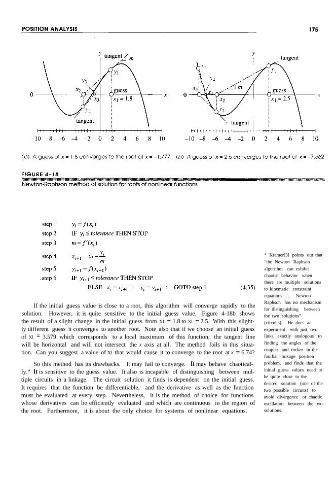
If the initial guess value is close to a root, this algorithm will converge rapidly to thesolution. However, it is quite sensitive to the initial guess value. Figure 4-18b showsthe result of a slight change in the initial guess from Xl = 1.8 to Xl = 2.5. With this slight-ly different guess it converges to another root. Note also that if we choose an initial guessof Xl = 3.579 which corresponds to a local maximum of this function, the tangent linewill be horizontal and will not intersect the X axis at all. The method fails in this situa-tion. Can you suggest a value of Xl that would cause it to converge to the root at X = 6.74?
So this method has its drawbacks. It may fail to converge. It may behave chaotical-ly.* It is sensitive to the guess value. It also is incapable of distinguishing between mul-tiple circuits in a linkage. The circuit solution it finds is dependent on the initial guess.It requires that the function be differentiable, and the derivative as well as the functionmust be evaluated at every step. Nevertheless, it is the method of choice for functionswhose derivatives can be efficiently evaluated and which are continuous in the region ofthe root. Furthermore, it is about the only choice for systems of nonlinear equations.
* Kramer[3] points out that"the Newton Raphsonalgorithm can exhibitchaotic behavior whenthere are multiple solutionsto kinematic constraintequations .... NewtonRaphson has no mechanismfor distinguishing betweenthe two solutions"(circuits). He does anexperiment with just twolinks, exactly analogous tofinding the angles of thecoupler and rocker in thefourbar linkage positionproblem, and finds that theinitial guess values need tobe quite close to thedesired solution (one of thetwo possible circuits) toavoid divergence or chaoticoscillation between the twosolutions.


Equation Solvers
Some commercially available equation solver software packages include the ability todo a Newton-Raphson iterative solution on sets of nonlinear simultaneous equations.TKSolver* and Mathcaat are examples. TKSolver automatically invokes its Newton-Raphson solver when it cannot directly solve the presented equation set, provided thatenough guess values have been supplied for the unknowns. These equation solver toolsare quite convenient in that the user need only supply the equations for the system in"raw" form such as equation 4.4la. It is not necessary to arrange them into the Newton-Raphson algorithm as shown in the previous section. Lacking such a commercial equa-tion solver, you will have to write your own computer code to program the solution asdescribed above. Reference [5] is a useful aid in this regard. The CD-ROM includedwith this text contains example TKSolver files for the solution of this fourbar positionproblem as well as others.
4.14 REFERENCES
1 Waldron, K. J., and S. V.Sreenivasan. (1996). "A Studyof the Solvabilityof the PositionProblemfor Multi-CircuitMechanismsby Wayof Exampleof the Double ButterflyLinkage."Journal ofMechanical Design, 118(3), p. 390.
2 Chase, T. R., and J. A. Mirth. (1993). "Circuitsand Branches of Single-Degree-of-FreedomPlanarLinkages."Journal of Mechanical Design, 115, p. 223.
3 Kramer, G. (1992). Solving Geometric Constraint Systems: A Case Study in Kinematics. MITPress: Cambridge,pp. 155-158.
4 Press, W. H., et aI. (1986). Numerical Recipes: The Art of Scientific Computing. CambridgeUniversityPress:Cambridge,pp. 145-146.
5 Ibid, pp. 254-273.
4.15 PROBLEMS
4-1 A position vector is defined as having a length equal to your height in inches (orcentimeters). The tangent of its angle is defined as your weight in pounds (orkilograms) divided by your age in years. Calculate the data for this vector and:
a. Draw the position vector to scale on cartesian axes.b. Write an expression for the position vector using unit vector notation.c. Write an expression for the position vector using complex number notation, in both
polar and cartesian fonns.
4-2 A particle is traveling along an arc of 6.5-in radius. The arc center is at the origin of acoordinate system. When the particle is at position A, its position vector makes a 45°angle with the X axis. At position B, its vector makes a 75° angle with the X axis.
* Universal TechnicalDraw this system to some convenient scale and:
Systems, 1220 Rock St. a. Write an expression for the particle's position vector in position A using complex
Rockford, IL 61101, USA. number notation, in both polar and cartesian fonns.(800) 435-7887 b. Write an expression for the particle's position vector in position B using complex
number notation, in both polar and cartesian fonns.t Mathsoft, 201 Broadway, c. Write a vector equation for the position difference between points Band A. Sub-Cambridge, MA 02139 stitute the complex number notation for the vectors in this equation and solve for(800) 628-4223 the position difference numerically.
d. Check the result of part c with a graphical method.


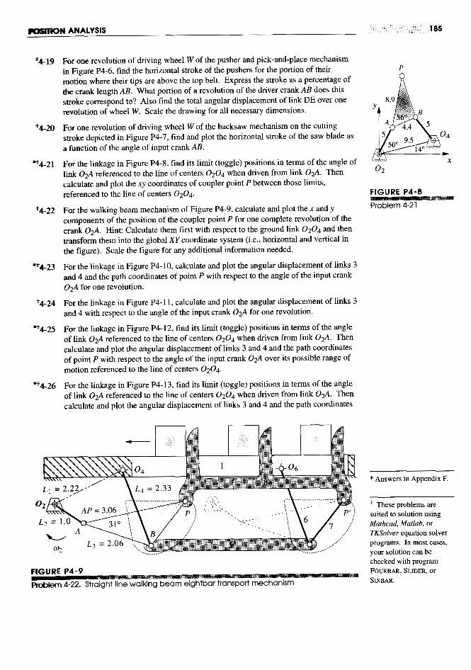
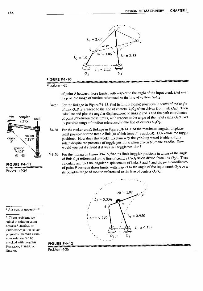


188
5.0 INTRODUCTION
With the fundamentals of position analysis established, we can now use these techniquesto synthesize linkages for specified output positions analytically. The synthesis tech-niques presented in Chapter 3 were strictly graphical and somewhat intuitive. The ana-lytical synthesis procedure is algebraic rather than graphical and is less intuitive. How-ever, its algebraic nature makes it quite suitable for computerization. These analyticalsynthesis methods were originated by Sandor[1] and further developed by his students,Erdman,[2] Kaufman,[3] and Loerch et aI.l4,S]
5.1 TYPESOF KINEMATIC SYNTHESIS
Erdman and Sandor[6] define three types of kinematic synthesis, function, path, andmotion generation, which were discussed in Section 3.2. Brief definitions are repeatedhere for your convenience.
FUNCTION GENERATION is defined as the correlation of an input function withan output function in a mechanism. Typically, a double-rocker or crank-rocker is theresult, with pure rotation input and pure rotation output. A slider-crank linkage can be afunction generator as well, driven from either end, i.e., rotation in and translation out orvice versa.
PATH GENERATION is defined as the control of a point in the plane such that itfollows some prescribed path. This is typically accomplished with a fourbar crank-rock-e~or double-rocker, wherein a point on the coupler traces the desired output path. No

attempt is made in path generation to control the orientation of the link which containsthe point of interest. The coupler curve is made to pass through a set of desired outputpoints. However, it is common for the timing of the arrival of the coupler point at partic-ular locations along the path to be defined. This case is called path generation with pre-scribed timing and is analogous to function generation in that a particular output func-tion is specified.
MOTION GENERATION is defined as the control of a line in the plane such that itassumes some sequential set of prescribed positions. Here orientation of the link con-taining the line is important. This is typically accomplished with a fourbar crank-rockeror double-rocker, wherein a point on the coupler traces the desired output path and thelinkage also controls the angular orientation of the coupler link containing the output lineof interest.
5.2 PRECISION POINTS
The points, or positions, prescribed for successive locations of the output (coupler orrocker) link in the plane are generally referred to as precision points or precision posi-tions. The number of precision points which can be synthesized is limited by the num-ber of equations available for solution. The fourbar linkage can be synthesized byclosed-form methods for up to five precision points for motion or path generation withprescribed timing (coupler output) and up to seven points for function generation (rock-er output). Synthesis for two or three precision points is relatively straightforward, andeach of these cases can be reduced to a system of linear simultaneous equations easilysolved on a calculator. The four or more position synthesis problems involve the solu-tion of nonlinear, simultaneous equation systems, and so are more complicated to solve,requiring a computer.
Note that these analytical synthesis procedures provide a solution which will be ableto "be at" the specified precision points, but no guarantee is provided regarding the link-age's behavior between those precision points. It is possible that the resulting linkagewill be incapable of moving from one precision point to another due to the presence of atoggle position or other constraint. This situation is actually no different than that of thegraphical synthesis cases in Chapter 3, wherein there was also the possibility of a toggleposition between design points. In fact, these analytical synthesis methods are just analternate way to solve the same multi position synthesis problems. One should still builda simple cardboard model of the synthesized linkage to observe its behavior and checkfor the presence of problems, even if the synthesis was performed by an esoteric analyt-ical method.
5.3 TWO-POSITION MOTION GENERATION BY ANALYTICALSYNTHESIS
Figure 5-1 shows a fourbar linkage in one position with a coupler point located at a firstprecision position Pl' It also indicates a second precision position (point Pz) to beachieved by the rotation of the input rocker, link 2, through an as yet unspecified angle~z. Note also that the angle of the coupler link 3 at each of the precision positions isdefined by the angles of the position vectors Zl and Zz. The angle <I> corresponds to the


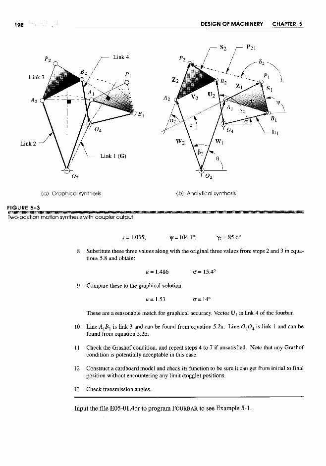


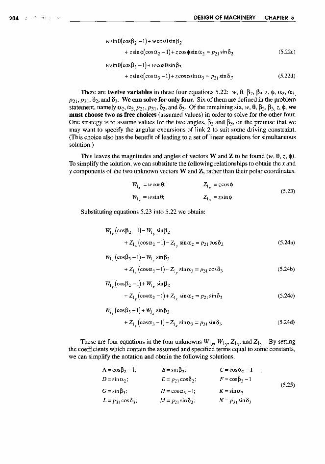


Equations 5.31 can be solved using the approach of equations 5.27 and 5.18, bychanging W to U and Z to S and using the definitions of the constants given in equation5.30 in equation 5.27.
It should be apparent that there are infinities of solutions to this three-position syn-thesis problem as well. An inappropriate selection of the two free choices could lead toa solution which has circuit, branch, or order problems in moving among all specifiedpositions. Thus we must check the function of the solution synthesized by this or anyother method. A simple model is the quickest check.
5.7 COMPARISON OF ANALYTICAL AND GRAPHICAL THREE-POSITION SYNTHESIS
Figure 5-5 shows the same three-position synthesis problem as was done graphically inExample 3-6 in Section 3.4. Compare this figure to Figure 3-9. The labeling has beenchanged to be consistent with the notation in this chapter. The points PJ, Pz, and P3 cor-respond to the three points labeled D in the earlier figure. Points AI, Az, and A3 corre-spond to points E; points B 1, Bz, and B3 correspond to points F. The old line AP becomesthe present Z vector. Point P is the coupler point which will go through the specifiedprecision points, PJ, Pz, and P3. Points A and B are the attachment points for the rockers(links 2 and 4, respectively) on the coupler (link 3). We wish to solve for the coordinatesof vectors W, Z, D, and S, which define not only the lengths of those links but also thelocations of the fixed pivots Oz and 04 in the plane and the lengths oflinks 3 and 1. Link1 is defined as vector G in Figure 5-4 (p. 202) and can be found from equation 5.2b (p.191). Link 3 is vector V found from equation 5.2a.
Four free choices must be made to constrain the problem to a particular solution outof the infinities of solutions available. In this case the values of link angles ~z, ~3' Yz,and Y3 have been chosen to be the same values as those which were found in the graph-ical solution to Example 3-6 in order to obtain the same solution as a check and compar-ison. Recall that in doing the graphical three-position synthesis solution to this sameproblem we in fact also had to make four free choices. These were the x,y coordinates ofthe moving pivot locations E and F in Figure 3-9 which correspond in concept to our fourfree choices of link angles here.


The angles <xz and <X3 must be measured from the diagram and supplied, in degrees.These six items constitute the set of "givens." Note that these data are all relative in-formation relating the second and third positions to the first. No information abouttheir absolute locations is needed. The global reference system can be taken to be any-where in the plane. We took it to be at the first precision point position PI for conve-nience. The free choices ~z and ~3 for the first dyad and "fz, "f3 for the second dyad mustalso be input to program FOURBARas they also were to program MATRIX.
Program FOURBARthen solves the matrix equation 5.27 once with the values fromequation 5.25 inserted to get the coordinates of vectors W and Z, and a second time withvalues from equation 5.31 in the matrix to get the coordinates of vectors U and S. Equa-tions 5.2 are then solved to find links 1 and 3, and the appropriate vector components areadded together to get the locations of fixed pivots Oz and 04. The link lengths are re-turned to the main part of program FOURBARso that other linkage parameters can becalculated and the linkage animated.
Note that there are two ways to assemble any fourbar linkage, open and crossed (seeFigure 4-8, p.155), and this analytical synthesis technique gives no information on whichmode of assembly is necessary to get the desired solution. Thus you may have to try bothmodes of assembly in program FOURBARto find the correct one after determining theproper link lengths with this method. Note also that program FOURBARalways draws


22<4 DESIGN OF MACHINERY CHAPTER 5
5.13 OTHER LINKAGE SYNTHESIS METHODS
Many other techniques for the synthesis of linkages to provide a prescribed motion havebeen created or discovered in recent years. Most of these approaches are somewhat in-volved and many are mathematically complicated. Only a few allow a closed-form so-lution; most require an iterative numerical solution. Most address the path synthesisproblem with or without concern for prescribed timing. As Erdman and Sandor pointout, the path, motion, and function generation problems are closely related.[6]
Space does not permit a complete exposition of even one of these approaches in thistext. We choose instead to present brief synopses of a number of synthesis methodsalong with complete references to their full descriptions in the engineering and scientif-ic literature. The reader interested in a detailed account of any method listed may con-sult the referenced papers which can be obtained through any university library or largepublic library. Also, some of the authors of these methods may make copies of their com-puter code available to interested parties.
Table 5-5 summarizes some of the existing fourbar linkage synthesis methods andfor each one lists the method type, the maximum number of positions synthesized, theapproach, special features, and a bibliographic reference (see the end of this chapter forthe complete reference). The list in Table 5-5 is not exhaustive; other methods than thesealso exist.
The listed methods are divided into three types labeled precision, equation, and op-timized (first column of Table 5-5). By precision (from precision point) is meant amethod, such as the ones described in previous sections of this chapter, that attempts tofind a solution which will pass exactly through the desired (precision) points but maydeviate from the desired path between these points. Precision point methods are limitedto matching a number of points equal to the number of independently adjustable param-eters that define the mechanism. For a fourbar linkage, this is nine. * (Higher-order link-ages with more links and joints will have a larger number of possible precision points.)
For up to 5 precision points in the fourbar linkage, the equations can be solved inclosed form without iteration. (The four-point solution is used as a tool to solve for 5positions in closed form, but for 6 points or more the nonlinear equations are difficult tohandle.) For 6 to 9 precision points an iterative method is needed to solve the equationset. There can be problems of nonconvergence, or convergence to singular or imaginarysolutions, when iterating nonlinear equations. Regardless of the number of points solvedfor, the solution found may be unusable due to circuit, branch, or order (CBO) defects. Acircuit defect means that the linkage must be disassembled and reassembled to reachsome positions, and a branch defect means that a toggle position is encountered between
* The nine independentsuccessive positions (see Section 4.12, p. 173). An order defect means that the points
parameters of a fourbarare all reachable on the same branch but are encountered in the wrong order.
linkage are: four link The type labeled equation in Table 5-5 refers to methods that solve the tricircular,lengths, two coordinates of trinodal sextic coupler curve to find a linkage that will generate an entire coupler curvethe coupler point with that closely approximates a set of desired points on the curve.respect to the coupler link,and three parameters that The type labeled optimized in Table 5-5 refers to an iterative optimization proce-define the location and dure that attempts to minimize an objective function that can be defined in many ways,orientation of the fixed linkin the global coordinate such as the least-squares deviation between the calculated and desired coupler point po-system.

sitions, for example. The calculated points are found by solving a set of equations thatdefine the behavior of the linkage geometry, using assumed initial values for the linkageparameters. A set of inequality constraints that limit the range of variation of parameterssuch as link length ratios, Grashof condition, or transmission angle may also be includ-ed in the calculation. New values of linkage parameters are generated with each itera-tion step according to the particular optimization scheme used. The closest achievablefit between the calculated solution points and the desired points is sought, defined asminimization of the chosen objective function. None of the desired points will be exact-ly matched by these methods, but for most engineering tasks this is an acceptable result.

Optimization methods allow larger numbers of points to be specified than do theprecision methods, limited only by available computer time and numerical roundoff er-ror. Table 5-5 shows a variety of optimization schemes ranging from the mundane (leastsquares) to the esoteric (fuzzy logic, genetic algorithms). All require a computer-pro-grammed solution. Most can be run on current desktop computers in reasonably shorttimes. Each different optimization approach has advantages and disadvantages in respectto convergence, accuracy, reliability, complexity, speed, and computational burden.Convergence often depends on a good choice of initial assumptions (guess values) forthe linkage parameters. Some methods, if they converge at all, do so to a local minimum(only one of many possible solutions), and it may not be the best one for the task.
Precision Point Methods
Table 5-5 shows several precision point synthesis methods. Some of these are based onoriginal work by Freudenstein and SandorJIO] Sandor [1] and Erdman [2], [6]developedthis approach into the "standard form" which is described in detail in this chapter. Thismethod yields closed-form solutions for 2, 3, and 4 precision positions and is extendableto 5 positions. It suffers from the possible circuit, branch, and order (CBO) defects com-mon to all precision point methods.
The method of Suh and Radcliffe [II] is similar to that of Freudenstein and others [1],
[2], [6],[10] but leads to a set of simultaneous nonlinear equations which are solved for upto 5 positions using the Newton-Raphson numerical method (see Section 4.13, p. 174).This approach adds to the usual CBO problems the possibilities of nonconvergence, orconvergence to singular or imaginary solutions.
Recent developments in the mathematical theory of polynomials have created newmethods of solution called continuation methods (also called homotopy methods)which do not suffer from the same convergence problems as other methods and can alsodetermine all the solutions of the equations starting from any set of assumed val-ues. [12], [13] Continuation methods are a general solution to this class of problem andare reliable and fast enough to allow multiple designs to be investigated in a reasonabletime (typically measured in CPU hours on a powerful computer).
Several researchers have developed solutions for the 5- to 9-precision point prob-lem using this technique. Morgan and Wampler [14] solved the fourbar linkage 5-pointproblem with specified fixed pivots completely and found a maximum of 36 real solu-tions. Subbian and Flugrad [15] used specified moving pivots for the 5-point problem,extended the 5-point method to sixbar linkages,D6] and also synthesized eightbar andgeared fivebar mechanisms for 6 and 7 precision points using continuation methods. [17]
Only the continuation method has yet been able to completely solve the fourbar link-age 9-precision-point problem and yield all its possible solutions. Wampler, Morgan, andSommese [18] used a combination of analytical equation reduction and numerical con-tinuation methods to exhaustively compute all possible nondegenerate, generic solutionsto the 9-point problem. * They proved that there is a maximum of 4326 distinct, nonde-generate linkages (occurring in 1442 sets of cognate triples) that will potentially solve ageneric 9-precision-point fourbar problem. Their method does not eliminate physicallyimpossible (complex link) linkages or those with CBO defects. These still have to beremoved by examination of the various solutions. They also solved four examples and

found the maximum number of linkages with real link lengths that generated these par-ticular 9-point paths to be, respectively, 21, 45, 64, and 120 cognate triples. Computa-tion times ranged from 69 to 321 CPV minutes on an IBM 3090 for these four examples.
Tylaska and Kazerounian [19],[20]took a different approach and devised a methodthat synthesizes a fourbar linkage for up to 7 precision points and also synthesized a WattI sixbar linkage for up to six body guidance (motion specification) positions with con-trol over locations of some ground and moving pivots. Their method yields the entireset of solutions for any set of design data and is an improvement over iterative methodsthat are sensitive to initial guesses. It is less computationally intensive than the continu-ation methods.
Coupler Curve Equation Methods
Blechschmidt and Vicker [21]and Ananthasuresh and Kota [22]used the algebraic cou-pler curve equation rather than a vector loop approach to calculate the coupler point path.The equation of the coupler curve is a tricircular, trinodal sextic of 15 terms. Nolle [23]states that:
The coupler curve equation itself is very complex and as far as is known in the study of me-chanics (or for that matter elsewhere) no other mathematical result has been found havingalgebraic characteristics matching those of the coupler curve.
Its solution is quite involved and requires iteration. Blechschmidt and Vicker's ap-proach [21]chose coordinates for 10 points on the desired curve. Ananthasuresh used 15points with some trial and error required in their selection. The advantage of these cou-pler curve equation approaches is that they define the entire curve which can be plottedand examined for suitability and defects prior to calculating the link dimensions whichrequires significant additional computing time.
Optimization Methods
The methods listed as optimized in Table 5-5 are a diverse group and some have little incommon except the goal of finding a linkage that will generate a desired path. All allowa theoretically unlimited number of design points to be specified, but making N too largewill increase the computation time and may not improve the result. One inherent limita-tion of optimization methods is that they may converge to a local minimum near the start-ing conditions. The result may not be as good as other minima located elsewhere in theN-space of the variables. Finding the global optimum is possible but more difficult andtime consuming.
Perhaps the earliest application (1966) of optimization techniques to this fourbarlinkage path synthesis problem is that of Fox and Willmert [24]in which they minimizedthe area between the desired and calculated curves subject to a number of equality andinequality constraints. They controlled link lengths to be positive and less than somemaximum, controlled for Grashof condition, limited forces and torques, and restrictedthe locations of the fixed pivots. They used Powell's method to find the minimum of theobjective function.
Youssef et al.,[25] used sum of squares, sum of absolute values, or area error criteriato minimize the objective function. They accommodated path and function generation

for single-loop (fourbar) or multiloop (more than four bar) linkages with both pin andslider joints. They allowed constraints to be imposed on the allowable ranges of linklengths and angles, any of which also may be held constant during the iteration. An ex-ample of an optimization done with this method for 19 evenly spaced points around adesired fourbar coupler path is shown in Figure 5-11 P5] Another example of this meth-od is the lO-bar crank-slider linkage in Figure 5-12 [25] which also shows the desired andactual coupler curve generated by point P for 24 points corresponding to equal incre-ments of input crank angle.
Nolle and Hunt [9] derived analytical expressions that lead to a set of ten linear si-multaneous nonhomogeneous equations whose solution gives values for all the indepen-dent variables. They used a least squares approach to the optimization and also allowedspecified timing of the input crank to each position on the coupler. Because their equa-tions are linear, convergence is rapid requiring only about one second per iteration.
Kramer and Sandor [26], [27] described a variant on the precision point techniquewhich they call selective precision synthesis (SPS). It relaxes the requirement that thecurve pass exactly through the precision points by defining "accuracy neighborhoods"around each point. The size of these tolerance zones can be different for each point, andmore than nine points can be used. They point out that exact correspondence to a set ofpoints is often not necessary in engineering applications and even if achieved theoreti-cally would be compromised by manufacturing tolerances.
The SPS approach is suitable to any linkage constructible from dyads or triads andso can accommodate sixbar and geared fivebar linkages as well as fourbars. Fourbarfunction, motion, or path generation (with prescribed timing) can all be synthesized, us-ing the standard form approach which considers all three forms equivalent in terms ofequation formulation. Spatial mechanisms can also be accommodated. The solutionsare stable and less sensitive to small changes in the data than precision point methods.Krishnamurthi et al.P8] extended the SPS approach by using fuzzy set theory whichgives a mechanism path as close to the specified points as is possible for a given startpoint; but it is sensitive to start point selection and may find local optima rather thanglobal.
Mirth [29] provided a variation on Kramer's SPS technique called quasi-precisionposition synthesis which uses three precision positions and N quasi positions which aredefined as tolerance zones. This approach retains the computational advantages of theBurmester (precision point) approach while also allowing the specification of a largernumber of points to improve and refine the design.
Conte et al., [30] and Kakatsios and Tricamo [31], [32] described methods to satisfy asmall number of precision points and simultaneously optimize the linkage's dynamiccharacteristics. The link lengths are controlled to reasonable size, the Grashof conditionconstrained, and the input torque, dynamic bearing and reaction forces, and shakingmoments simultaneously minimized.
Many of the optimization methods listed above use some form of inequality con-straints to limit the allowable values of design parameters such as link lengths and trans-mission angles. These constraints often cause problems that lead to nonconvergence, orto CBO defects. Angeles et al., [33] described an unconstrained nonlinear least-square-method that avoids these problems. Continuation methods are employed, and good con-vergence is claimed with no branch defects.

Aviles et aI., [34] proposed a novel approach to the linkage synthesis problem thatuses the elastic energy that would be stored in the links if they were allowed to deformelastically such that the coupler point reaches the desired location. The objective func-tion is defined as the minimum energy condition in the set of deformed links which ofcourse will occur when their rigid body positions most closely approach the desired path.This is essentially a finite element method approach that considers each link to be a barelement. Newton's method is used for the iteration and, in this case, converges to a min-imum even when the initial guess is far from a solution.
Fang [35] described an unusual approach to linkage synthesis using genetic algo-rithms. Genetic algorithms emulate the way that living organisms adapt to nature. Ini-tially, a population of random "organisms" are generated that represent the system to beoptimized. This takes the form of a bit string, analogous to a cell's chromosomes whichis called the first generation. Two operations are performed on a given population, calledcrossover and mutation. Crossover combines part of the "genetic code" of a "father" or-ganism with part of the code of a "mother" organism. Mutation changes values of thegenetic code at random points in the bit string. An objective function is created that ex-presses the "fitness" of the organism for the desired task. Each successive generation is

produced by selecting the organisms that best fit the task. The population "evolves"through generations until a termination criterion is met based on the objective function.
Some advantages of this approach are that it searches from population to populationrather than point to point, and this makes it less likely to be trapped at local optima. Thepopulation also preserves a number of valid solutions rather than converging to only one.The disadvantages are long computation times due to the large number of objective func-tion evaluations required. Nevertheless it is more efficient than random walk or exhaus-tive search algorithms. All other optimization approaches listed here deal only with di-mensional synthesis, but genetic algorithms can also deal with type synthesis.
Ullah and Kota [36], [37] separated the linkage synthesis problem into two steps. Thefirst step seeks an acceptable match for the shape of the desired curve without regard tothe size, orientation, or location of the curve in space. Once a curve of suitable shapeand its associated linkage are found, the result can be translated, rotated, and scaled asdesired. This approach simplifies the optimization task compared to the algorithms thatseek a structural optimization that includes size, orientation, and location of the couplercurve all at once in the objective function. Fourier descriptors are used to characterizethe shape of the curve as is done in many pattern matching applications such as for auto-mated robotic assembly tasks. A stochastic global optimization algorithm is used whichavoids unwanted convergence to suboptimal local minima.
Bawab et aI., [38] described an approach that will automatically (within the softwareprogram) synthesize a fourbar linkage for two, three, or four positions using Burmestertheory and eliminate all solutions having CBO defects. Limits on link length ratios andtransmission angle are specified and the objective function is based on these criteria withweighting factors applied. Regions in the plane within which the fixed or moving pivotsmust be located may also be specified.

8 Erdman, A. G., and J. E. Gustafson. (1977). "LINCAGES: Linkage INteractiveComputer Analysis and Graphically Enhanced Synthesis." ASME Paper: 77-DTC-5.
9 Nolle, H., and K. H. Hunt. (1971). "Optimum Synthesis of Planar Linkages toGenerate Coupler Curves." Journal of Mechanisms, 6, pp. 267-287.
10 Freudenstein, F., and G. N. Sandor. (1959). "Synthesis of Path GeneratingMechanisms by Means of a Programmed Digital Computer." ASME Journal forEngineering in Industry, 81, p. 2.
11 Suh, C. H., and C. W. Radcliffe. (1966). "Synthesis of Planar Linkages With Use ofthe Displacement Matrix." ASME Paper: 66-MECH-19. 9 pp.
12 Morgan, A. P., and A. J. Sommese. (1987). "Computing all Solutions to PolynomialSystems Using Homotopy Continuation." Applied Mathematics and Computation, 24,pp. ll5-138.
13 Morgan, A. P. (1987). Solving Polynomial Systems Using Continuation for Scientificand Engineering Problems. Prentice-Hall: Upper Saddle River, NJ.
14 Morgan, A. P., and C. W. Wampler. (1990). "Solving a Planar Fourbar DesignProblem Using Continuation." Journal of Mechanical Design, 112(4), p. 544.
15 Subbian, T., and J. D. R. Flugrad. (1991). "Fourbar Path Generation Synthesis by aContinuation Method." Journal of Mechanical Design, 113(1), p. 63.
16 Subbian, T., and J. D. R. Flugrad. (1993). "Five Position Triad Synthesis withApplications to Four and Sixbar Mechanisms." Journal of Mechanical Design,115(2), p. 262.
17 Subbian, T., and J. D. R. Flugrad. (1994). "Six and Seven Position Triad SynthesisUsing Continuation Methods." Journal of Mechanical Design, 116(2), p. 660.
18 Wampler, C. W., et a!. (1992). "Complete Solution of the Nine-Point Path SynthesisProblem for Fourbar Linkages." Journal of Mechanical Design, 114(1), p. 153.
19 Tylaska, T., and K. Kazerounian. (1994). "Synthesis of Defect-Free SixbarLinkages for Body Guidance Through Up to Six Finitely Separated positions." Proc.of 23rd Biennial Mechanisms Conference, Minneapolis, MI, p. 369.
20 Tylaska, T., and K. Kazerounian. (1993). "Design of a Six Position Body GuidanceWatt I Sixbar Linkage and Related Concepts." Proc. of 3rd Applied Mechanisms andRobotics Conference, Cincinnati, pp. 93-1.
21 Blechschmidt, J. L., and J. J. Vicker. (1986). "Linkage Synthesis Using AlgebraicCurves." J. Mechanisms, Transmissions, and Automation in Design, 108 (December1986), pp. 543-548.
22 Ananthasuresh, G. K., and S. Kota. (1993). "A Renewed Approach to the Synthesisof Fourbar Linkages for Path Generation via the Coupler Curve Equation." Proc. of3rd Applied Mechanisms and Robotics Conference, Cincinnati, pp. 83-1.
23 Nolle, H. (1975). "Linkage Coupler Curve Synthesis: A Historical Review - III.Spatial Synthesis and Optimization." Mechanism and Machine Theory, 10, 1975, pp.41-55.
24 Fox, R. L., and K. D. Willmert. (1967). "Optimum Design of Curve-GeneratingLinkages with Inequality Constraints." Journal of Engineering for Industry (Feb1967), pp. 144-152.

25 Youssef, A. H., et at. (1975). "Optimal Kinematic Synthesis of Planar LinkageMechanisms." I. Mech. E., pp. 393-398.
26 Kramer, S. N., and G. N. Sandor. (1975). "Selective Precision Synthesis-AGeneral Method of Optimization for Planar Mechanisms." Trans ASME J. Eng. forIndustry, 97B(2), pp. 689-701.
27 Kramer, S. N. (1987). "Selective Precision Synthesis-A General Design Method forPlanar and Spatial Mechanisms." Proc. of 7th World Congress on Theory of Machinesand Mechanisms, Seville Spain.
28 Krishnamurthi, S., et at. (1993). "Fuzzy Synthesis of Mechanisms." Proc. of 3rdApplied Mechanisms and Robotics Conference, Cincinnati, pp. 94-1.
29 Mirth, J. A. (1994). "Quasi-Precision Position Synthesis of Fourbar Linkages." Proc.of 23rd Biennial Mechanisms Conference, Minneapolis, MI, p. 215.
30 Conte, F. L., et at. (1975). "Optimum Mechanism Design Combining Kinematic andDynamic-Force Considerations." Journal of Engineering for Industry (May 1975),pp. 662-670.
31 Kakatsios,A. J., and S. J. Tricamo. (1987). "Precision Point Synthesis of Mecha-nisms with Optimal Dynamic Characteristics." Proc. of 7th World Congress on theTheory of Machines and Mechanisms, Seville, Spain, pp. 1041-1046.
32 Kakatsios, A. J., and S. J. Tricamo. (1986). "Design of Planar Rigid Body GuidanceMechanisms with Simultaneously Optimized Kinematic and Dynamic Characteris-tics." ASME Paper: 86-DET-142.
33 Angeles, J., et at. (1988). "An Unconstrained Nonlinear Least-Square Method ofOptimization of RRRR Planar Path Generators." Mechanism and Machine Theory,23(5), pp. 343-353.
34 Aviles, R., et al. (1994). "An Energy-Based General Method for the OptimumSynthesis of Mechanisms." Journal of Mechanical Design, 116(1), p. 127.
35 Fang, W. E. (1994). "Simultaneous Type and Dimensional Synthesis of Mechanismsby Genetic Algorithms." Proc. of 23rd Biennial Mechanisms Conference, Minneapo-lis, MI, p. 36.
36 Ullah, I., and S. Kota. (1994). "A More Effective Formulation of the Path Genera-tion Mechanism Synthesis Problem." Proc. of 23rd Biennial Mechanisms Conference,Minneapolis, Minn, p. 239.
37 Ullah, I., and S. Kota. (1996). "Globally-Optimal Synthesis of Mechanisms for PathGeneration using Simulated Annealing and Powell's Method." Proc. of ASME DesignEngineering Conference, Irvine, CA, pp. 1-8.
38 Bawab, S., et at. (1997). "Automatic Synthesis of Crank Driven Fourbar Mecha-nisms for Two, Three, or Four Position Motion Generation." Journal of MechanicalDesign, 119(June), pp. 225-231.
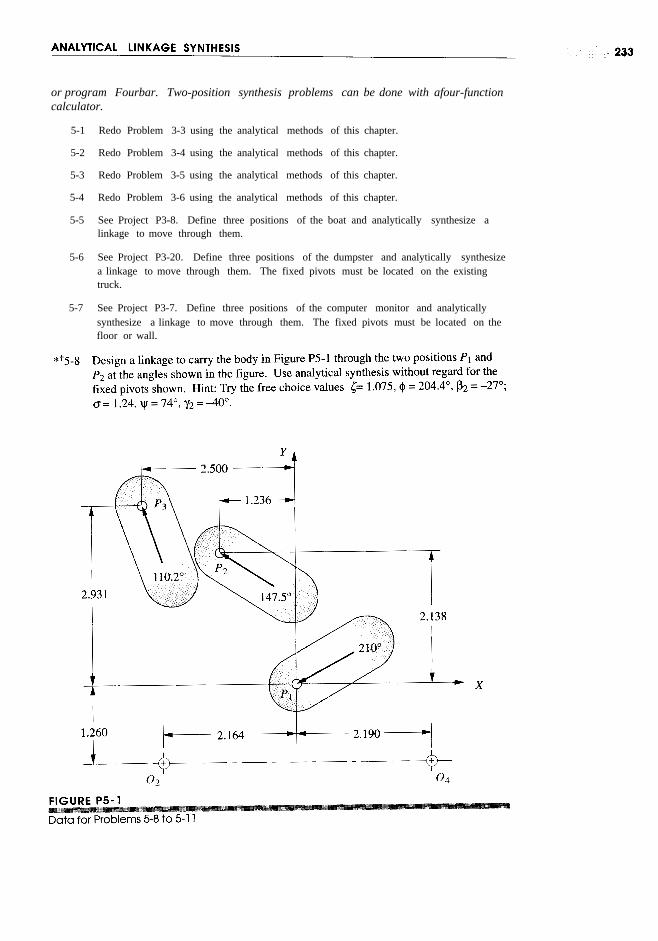
or program Fourbar. Two-position synthesis problems can be done with afour-functioncalculator.
5-1 Redo Problem 3-3 using the analytical methods of this chapter.
5-2 Redo Problem 3-4 using the analytical methods of this chapter.
5-3 Redo Problem 3-5 using the analytical methods of this chapter.
5-4 Redo Problem 3-6 using the analytical methods of this chapter.
5-5 See Project P3-8. Define three positions of the boat and analytically synthesize alinkage to move through them.
5-6 See Project P3-20. Define three positions of the dumpster and analytically synthesizea linkage to move through them. The fixed pivots must be located on the existingtruck.
5-7 See Project P3-7. Define three positions of the computer monitor and analyticallysynthesize a linkage to move through them. The fixed pivots must be located on thefloor or wall.


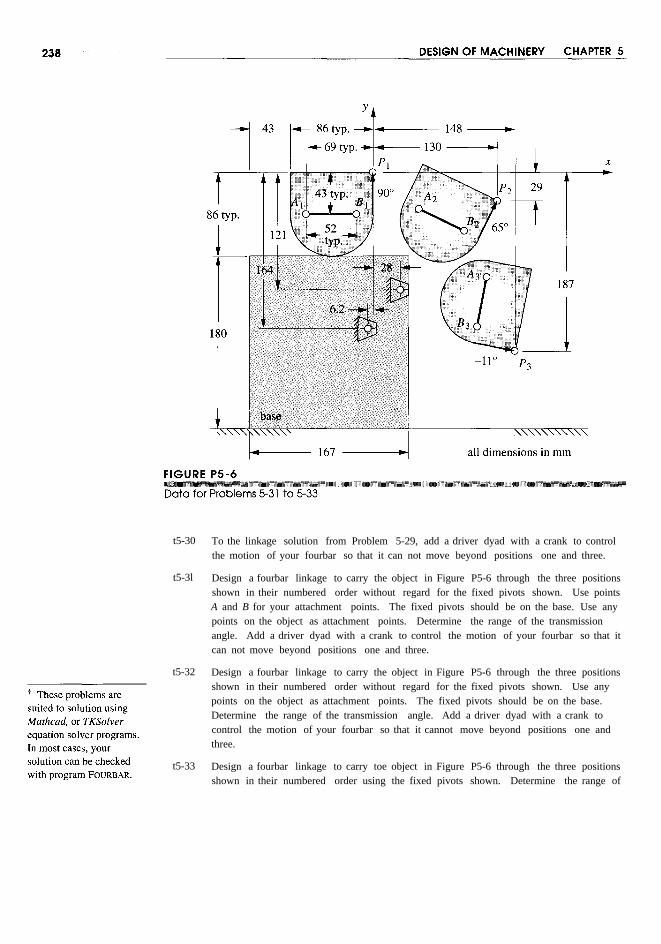
t5-30 To the linkage solution from Problem 5-29, add a driver dyad with a crank to controlthe motion of your fourbar so that it can not move beyond positions one and three.
t5-3l Design a fourbar linkage to carry the object in Figure P5-6 through the three positionsshown in their numbered order without regard for the fixed pivots shown. Use pointsA and B for your attachment points. The fixed pivots should be on the base. Use anypoints on the object as attachment points. Determine the range of the transmissionangle. Add a driver dyad with a crank to control the motion of your fourbar so that itcan not move beyond positions one and three.
t5-32 Design a fourbar linkage to carry the object in Figure P5-6 through the three positionsshown in their numbered order without regard for the fixed pivots shown. Use anypoints on the object as attachment points. The fixed pivots should be on the base.Determine the range of the transmission angle. Add a driver dyad with a crank tocontrol the motion of your fourbar so that it cannot move beyond positions one andthree.
t5-33 Design a fourbar linkage to carry toe object in Figure P5-6 through the three positionsshown in their numbered order using the fixed pivots shown. Determine the range of


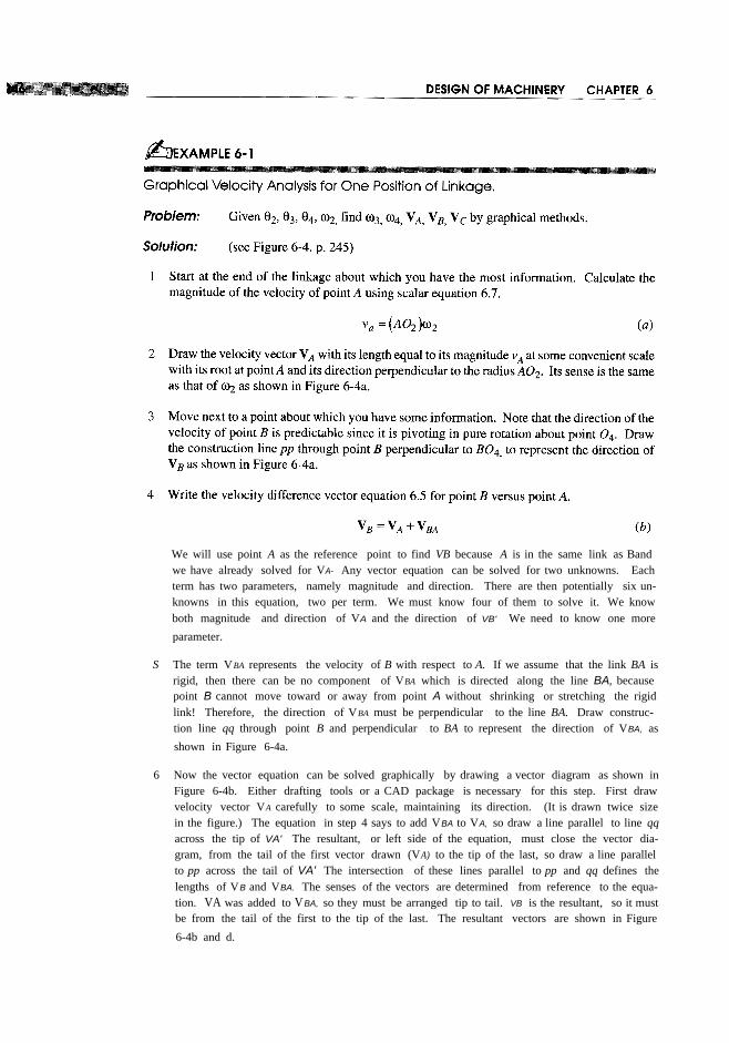
We will use point A as the reference point to find VB because A is in the same link as Bandwe have already solved for VA- Any vector equation can be solved for two unknowns. Eachterm has two parameters, namely magnitude and direction. There are then potentially six un-knowns in this equation, two per term. We must know four of them to solve it. We knowboth magnitude and direction of VA and the direction of VB' We need to know one moreparameter.
S The term VBA represents the velocity of B with respect to A. If we assume that the link BA isrigid, then there can be no component of VBA which is directed along the line BA, becausepoint B cannot move toward or away from point A without shrinking or stretching the rigidlink! Therefore, the direction of VBA must be perpendicular to the line BA. Draw construc-tion line qq through point B and perpendicular to BA to represent the direction of VBA, asshown in Figure 6-4a.
6 Now the vector equation can be solved graphically by drawing a vector diagram as shown inFigure 6-4b. Either drafting tools or a CAD package is necessary for this step. First drawvelocity vector VA carefully to some scale, maintaining its direction. (It is drawn twice sizein the figure.) The equation in step 4 says to add VBA to VA, so draw a line parallel to line qqacross the tip of VA' The resultant, or left side of the equation, must close the vector dia-gram, from the tail of the first vector drawn (VA) to the tip of the last, so draw a line parallelto pp across the tail of VA' The intersection of these lines parallel to pp and qq defines thelengths of VB and VBA. The senses of the vectors are determined from reference to the equa-tion. VA was added to VBA, so they must be arranged tip to tail. VB is the resultant, so it mustbe from the tail of the first to the tip of the last. The resultant vectors are shown in Figure6-4b and d.


which the motion was pure rotation so that one of the terms in equation 6.5 (p. 243)would be zero. (We could as easily have looked for a point in pure translation to boot-strap the solution.) We then solved for the absolute velocity of that point (VA) usingequations 6.5 and 6.7 (p. 244). (Steps I and 2)
We then used the point (A) just solved for as a reference point to define the transla-tion component in equation 6.5 written for a new point (B). Note that we needed tochoose a second point (B) which was in the same rigid body as the reference point (A)which we had already solved and about which we could predict some aspect of the newpoint's (B's) velocity. In this example, we knew the direction of the velocity VB. Ingeneral this condition will be satisfied by any point on a link which is jointed to ground(as is link 4). In this example, we could not have solved for point C until we solved forB, because point C is on a floating link for which point we do not yet know the velocitydirection. (Steps 3 and 4)
To solve the equation for the second point (B), we also needed to recognize that therotation component of velocity is directed perpendicular to the line connecting the twopoints in the link (B and A in the example). You will always know the direction of therotation component in equation 6.5 if it represents a velocity difference (CASE 1) sit-uation. If the rotation component relates two points in the same rigid body, then thatvelocity difference component is always perpendicular to the line connecting those twopoints (see Figure 6-2, p. 243). This will be true regardless of the two points selected.But, this is not true in a CASE 2 situation (see Figure 6-3, p. 244). (Steps 5 and 6)
Once we found the absolute velocity (VB) of a second point on the same link (CASE1) we could solve for the angular velocity of that link. (Note that points A and Bareboth on link 3 and the velocity of point 04 is zero.) Once the angular velocities of all thelinks were known, we could solve for the linear velocity of any point (such as C) in anylink using equation 6.5. To do so, we had to understand the concept of angular velocityas a free vector, meaning that it exists everywhere on the link at any given instant. Ithas no particular center. It has an infinity of potential centers. The link simply has anangular velocity, just as does a frisbee thrown and spun across the lawn.
All points on afrisbee, if spinning while flying, obey equation 6.5. Left to its owndevices, the frisbee will spin about its center of gravity (CG), which is close to the centerof its circular shape. But if you are an expert frisbee player (and have rather pointed fin-gers), you can imagine catching that flying frisbee between your two index fingers insome off-center location (not at the CG), such that the frisbee continues to spin aboutyour fingertips. In this somewhat far-fetched example of championship frisbee play, youwill have taken the translation component of the frisbee's motion to zero, but its inde-pendent rotation component will still be present. Moreover, it will now be spinning abouta different center (your fingers) than it was in flight (its CG). Thus this free vector ofangular velocity «(0) is happy to attach itself to any point on the body. The body still hasthe same 00, regardless of the assumed center of rotation. It is this property that allowsus to solve equation 6.5 for literally any point on a rigid body in complex motion refer-enced to any other point on that body. (Steps 7 and 8).

From equation 6.8b we can see that a fourbar linkage has 6 instant centers, a sixbarhas 15, and an eightbar has 28.
Figure 6-5 shows a fourbar linkage in an arbitrary position. It also shows a lineargraph * which is useful for keeping track of which lCs have been found. This particulargraph can be created by drawing a circle on which we mark off as many points as thereare links in our assembly. We will then draw a line between the dots representing thelink pairs each time we find an instant center. The resulting linear graph is the set of linesconnecting the dots. It does not include the circle which was used only to place the dots.This graph is actually a geometric solution to equation 6.8b, since connecting all thepoints in pairs gives all the possible combinations of points taken two at a time.
Some lCs can be found by inspection, using only the definition of the instant center.Note in Figure 6-5a that the four pin joints each satisfy the definition. They clearly musthave the same velocity in both links at all times. These have been labeled h,2, h,3, h,4,and h,4' The order of the subscripts is immaterial. Instant center h,l is the same as h,2.These pin joint lCs are sometimes called "permanent" instant centers as they remain inthe same location for all positions of the linkage. In general, instant centers will move tonew locations as the linkage changes position, thus the adjective instant. In this fourbarexample there are two more lCs to be found. It will help to use the Aronhold-Kennedytheorem,t also called Kennedy's rule, to locate them.
Kennedy's rule:Any three bodies in plane motion will have exactly three instant centers, and they will lieon the same straight line.
The first part of this rule is just a restatement of equation 6.8b for n = 3. It is thesecond clause in this rule that is most useful. Note that this rule does not require that thethree bodies be connected in any way. We can use this rule, in conjunction with the lin-ear graph, to find the remaining lCs which are not obvious from inspection. Figure 6.5bshows the construction necessary to find instant center 11,3. Figure 6-5c shows the con-struction necessary to find instant center h,4' The following example describes the pro-cedure in detail.

The presence of slider joints makes finding the instant centers a little more subtle asis shown in the next example. Figure 6-6a shows a fourbar slider-crank linkage. Notethat there are only three pin joints in this linkage. All pin joints are permanent instantcenters. But the joint between links I and 4 is a rectilinear, sliding full joint. A slidingjoint is kinematically equivalent to an infinitely long link, "pivoted" at infinity. Figure6-6b shows a nearly equivalent pin-jointed version of the slider-crank in which link 4 isa very long rocker. Point B now swings through a shallow arc which is nearly a straight

line. It is clear in Figure 6-6b that, in this linkage, h,4 is at pivot 04. Now imagine in-creasing the length of this long, link 4 rocker even more. In the limit, link 4 approachesinfinite length, the pivot 04 approaches infinity along the line which was originally thelong rocker, and the arc motion of point B approaches a straight line. Thus, a slider jointwill have its instant center at infinity along a line perpendicular to the direction of slid-ing as shown in Figure 6-6a.


See Figure 6-11 and compare equation 6.13e to equation 6.llf and its discussionunder angular velocity ratio above. Equation 6.l3e shows that for any choice of rin androut, the mechanical advantage responds to changes in angles v and /.l in opposite fashionto that of the angular velocity ratio. If the transmission angle /.l goes to zero (which wedon't want it to do), the mechanical advantage also goes to zero regardless of the amountof input force or torque applied. But, when angle v goes to zero (which it can and does,twice per cycle in a Grashof linkage), the mechanical advantage becomes infinite! Thisis the principle of a rock-crusher mechanism as shown in Figure 6-11. A quite moderateforce applied to link 2 can generate a huge force on link 4 to crush the rock. Of course,we cannot expect to achieve the theoretical output of infinite force or torque magnitude,as the strengths of the links and joints will limit the maximum forces and torques obtain-able. Another common example of a linkage which takes advantage of this theoreticallyinfinite mechanical advantage at the toggle position is a ViseGrip locking pliers (see FigureP6-2l, p. 296).
These two ratios, angular velocity ratio and mechanical advantage, provide use-ful, dimensionless indices of merit by which we can judge the relative quality of vari-ous linkage designs which may be proposed as solutions.
Using Instant Centers in linkage Design
In addition to providing a quick numerical velocity analysis, instant center analysis moreimportantly gives the designer a remarkable overview of the linkage's global behavior.It is quite difficult to mentally visualize the complex motion of a "floating" coupler linkeven in a simple fourbar linkage, unless you build a model or run a computer simulation.Because this complex coupler motion in fact reduces to an instantaneous pure rotationabout the instant center h,3, finding that center allows the designer to visualize the mo-tion of the coupler as a pure rotation. One can literally see the motion and the directionsof velocities of any points of interest by relating them to the instant center. It is only nec-essary to draw the linkage in a few positions of interest, showing the instant center loca-tions for each position.

Figure 6-12 shows a practical example of how this visual, qualitative analysis tech-nique could be applied to the design of an automobile rear suspension system. Most au-tomobile suspension mechanisms are either fourbar linkages or fourbar slider-cranks,with the wheel assembly carried on the coupler (as was also shown in Figure 3-19,p. 108). Figure 6-l2a shows a rear suspension design from a domestic car of 1970's vin-tage which was later redesigned because of a disturbing tendency to "bump steer," i.e.,turn the rear axle when hitting a bump on one side of the car. The figure is a view look-ing from the center of the car outward, showing the fourbar linkage which controls theup and down motion of one side of the rear axle and one wheel. Links 2 and 4 are pivot-ed to the frame of the car which is link 1. The wheel and axle assembly is rigidly at-tached to the coupler, link 3. Thus the wheel assembly has complex motion in the verti-cal plane. Ideally, one would like the wheel to move up and down in a straight verticalline when hitting a bump. Figure 6-12b shows the motion of the wheel and the new in-stant center (I1,3) location for the situation when one wheel has hit a bump. The velocityvector for the center of the wheel in each position is drawn perpendicular to its radius

from Ir,3. You can see that the wheel center has a significant horizontal component ofmotion as it moves up over the bump. This horizontal component causes the wheel cen-ter on that side of the car to move forward while it moves upward, thus turning the axle(about a vertical axis) and steering the car with the rear wheels in the same way that yousteer a toy wagon. Viewing the path of the instant center over some range of motiongives a clear picture of the behavior of the coupler link. The undesirable behavior of thissuspension linkage system could have been predicted from this simple instant centeranalysis before ever building the mechanism.
Another practical example of the effective use of instant centers in linkage design isshown in Figure 6-13, which is an optical adjusting mechanism used to position a mirrorand allow a small amount of rotational adjustment. [1] A more detailed account of thisdesign case study [2] is provided in Chapter 18. The designer, K. Towfigh, recognizedthat Ir,3 at point E is an instantaneous "fixed pivot" and will allow very small pure rota-tions about that point with very small translational error. He then designed a one-piece,plastic fourbar linkage whose "pin joints" are thin webs of plastic which flex to allowslight rotation. This is termed a compliant linkage, one that uses elastic deformationsof the links as hinges instead of pin joints. He then placed the mirror on the coupler at11,3. Even the fixed link 1 is the same piece as the "movable links" and has a small setscrew to provide the adjustment. A simple and elegant design.
6.5 CENTRODES
Figure 6-14 illustrates the fact that the successive positions of an instant center (or cen-tro) form a path of their own. This path, or locus, of the instant center is called the cen-trode. Since there are two links needed to create an instant center, there will be two cen-trodes associated with anyone instant center. These are formed by projecting the pathof the instant center first on one link and then on the other. Figure 6-14a shows the locusof instant center Ir,3 as projected onto link 1. Because link I is stationary, or fixed, thisis called the fixed centrode. By temporarily inverting the mechanism and fixing link 3


as the ground link, as shown in Figure 6-14b, we can move link 1 as the coupler andproject the locus of 11,3 onto link 3. In the original linkage, link 3 was the moving cou-pler, so this is called the moving centrode. Figure 6-l4c shows the original linkage withboth fixed and moving centrodes superposed.
The definition of the instant center says that both links have the same velocity at thatpoint, at that instant. Link 1 has zero velocity everywhere, as does the fixed centrode.So, as the linkage moves, the moving centrode must roll against the fixed centrode with-out slipping. If you cut the fixed and moving centrodes out of metal, as shown in Figure6-14d, and roll the moving centrode (which is link 3) against the fixed centrode (whichis link 1), the complex motion of link 3 will be identical to that of the original linkage.All of the coupler curves of points on link 3 will have the same path shapes as in the orig-inallinkage. We now have, in effect, a "linkless" fourbar linkage, really one composedof two bodies which have these centrode shapes rolling against one another. Links 2 and4 have been eliminated. Note that the example shown in Figure 6-14 is a non-Grashoffourbar. The lengths of its centrodes are limited by the double-rocker toggle positions.
All instant centers of a linkage will have centrodes. If the links are directly connect-ed by a joint, such as lz,3, 13,4, h,2, and 11,4, their fixed and moving centrodes will de-generate to a point at that location on each link. The most interesting centrodes are thoseinvolving links not directly connected to one another such as 11,3 and h,4. If we look atthe double-crank linkage in Figure 6-l5a in which links 2 and 4 both revolve fully, wesee that the centrodes of 11,3 form closed curves. The motion of link 3 with respect tolink 1 could be duplicated by causing these two centrodes to roll against one anotherwithout slipping. Note that there are two loops to the moving centrode. Both must rollon the single-loop fixed centrode to complete the motion of the equivalent double-cranklinkage.
We have so far dealt largely with the instant center 11,3. Instant center lz,4 involvestwo links which are each in pure rotation and not directly connected to one another. Ifwe use a special-case Grashoflinkage with the links crossed (sometimes called an anti-parallelogram linkage), the centrodes of lz,4 become ellipses as shown in Figure 6-l5b.To guarantee no slip, it will probably be necessary to put meshing teeth on each centrode.We then will have a pair of elliptical, noncircular gears, or gearset, which gives thesame output motion as the original double-crank linkage and will have the same varia-tions in the angular velocity ratio and mechanical advantage as the linkage had. Thuswe can see that gearsets are also just fourbar linkages in disguise. Noncircular gearsfind much use in machinery, such as printing presses, where rollers must be speeded andslowed with some pattern during each cycle or revolution. More complicated shapes ofnoncircular gears are analogous to cams and followers in that the equivalent fourbar link-age must have variable-length links. Circular gears are just a special case of noncircu-lar gears which give a constant angular velocity ratio and are widely used in all ma-chines. Gears and gearsets will be dealt with in more detail in Chapter 10.
In general, centrodes of crank-rockers and double- or triple-rockers will be opencurves with asymptotes. Centrodes of double-crank linkages will be closed curves. Pro-gram FOURBARwill calculate and draw the fixed and moving centrodes for any linkageinput to it. Input the datafiles F06-l4.4br, F06-15aAbr, and F06-l5bAbr into programFOURBARto see the centrodes of these linkage drawn as the linkages rotate.

A "linkless" linkage
A common example of a mechanism made of centrodes is shown in Figure 6-16a. Youhave probably rocked in a Boston or Hitchcock rocking chair and experienced the sooth-ing motions that it delivers to your body. You may have also rocked in a platfonn rockeras shown in Figure 6-16b and noticed that its motion did not feel as soothing.
There are good kinematic reasons for the difference. The platform rocker has a fixedpin joint between the seat and the base (floor). Thus all parts of your body are in purerotation along concentric arcs. You are in effect riding on the rocker of a linkage.
The Boston rocker has a shaped (curved) base, or "runners," which rolls against thefloor. These runners are usually not circular arcs. They have a higher-order curve con-tour. They are, in fact, moving centrodes. The floor is the fixed centrode. When oneis rolled against the other, the chair and its occupant experience coupler curve motion.Every part of your body travels along a different sixth-order coupler curve which pro-vides smooth accelerations and velocities and feels better than the cruder second-order(circular) motion of the platform rocker. Our ancestors, who carved these rocking chairs,

probably had never heard of fourbar linkages and centrodes, but they knew intuitivelyhow to create comfortable motions.
CUSpS
Another example of a centrode which you probably use frequently is the path of the tireon your car or bicycle. As your tire rolls against the road without slipping, the road be-comes a fixed centrode and the circumference of the tire is the moving centrode. Thetire is, in effect, the coupler of a linkless fourbar linkage. All points on the contact sur-face of the tire move along cycloidal coupler curves and pass through a cusp of zerovelocity when they reach the fixed centrode at the road surface as shown in Figure 6-17 a.All other points on the tire and wheel assembly travel along coupler curves which do nothave cusps. This last fact is a clue to a means to identify coupler points which will havecusps in their coupler curve. If a coupler point is chosen to be on the moving centrode atone extreme of its path motion (i.e., at one of the positions ofh,3), then it will have a cuspin its coupler curve. Figure 6-17b shows a coupler curve of such a point, drawn withprogram FOURBAR. The right end of the coupler path touches the moving centrode andas a result has a cusp at that point. So, if you desire a cusp in your coupler motion, manyare available. Simply choose a coupler point on the moving centrode of link 3. Read thediskfile F06-17bAbr into program FOURBARto animate that linkage with its couplercurve or centrodes. Note in Figure 6-14 (p. 264) that choosing any location of instantcenter Il,3 on the coupler as the coupler point will provide a cusp at that point.
6.6 VELOCITY OF SLIP
When there is a sliding joint between two links and neither one is the ground link, thevelocity analysis is more complicated. Figure 6-18 shows an inversion of the fourbarslider-crank mechanism in which the sliding joint is floating, i.e., not grounded. To solvefor the velocity at the sliding joint A, we have to recognize that there is more than onepoint A at that joint. There is a point A as part of link 2 (Az), a point A as part oflink 3(A3), and a point A as part of link 4 (A4). This is a CASE2 situation in which we have atleast two points belonging to different links but occupying the same location at a giveninstant. Thus, the relative velocity equation 6.6 (p. 243) will apply. We can usuallysolve for the velocity of at least one of these points directly from the known input infor-mation using equation 6.7 (p. 244). It and equation 6.6 are all that are needed to solve foreverything else. In this example link 2 is the driver, and 8z and OOz are given for the"freeze frame" position shown. We wish to solve for 004, the angular velocity of link 4,and also for the velocity of slip at the joint labeled A.
In Figure 6-18 the axis of slip is shown to be tangent to the slider motion and is theline along which all sliding occurs between links 3 and 4. The axis of transmission isdefined to be perpendicular to the axis of slip and pass through the slider joint at A. Thisaxis of transmission is the only line along which we can transmit motion or force acrossthe slider joint, except for friction. We will assume friction to be negligible in this ex-ample. Any force or velocity vector applied to point A can be resolved into two compo-nents along these two axes which provide a translating and rotating, local coordinatesystem for analysis at the joint. The component along the axis of transmission will douseful work at the joint. But, the component along the axis of slip does no work, exceptfriction work.


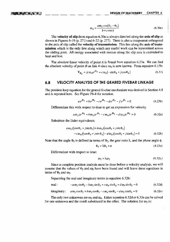

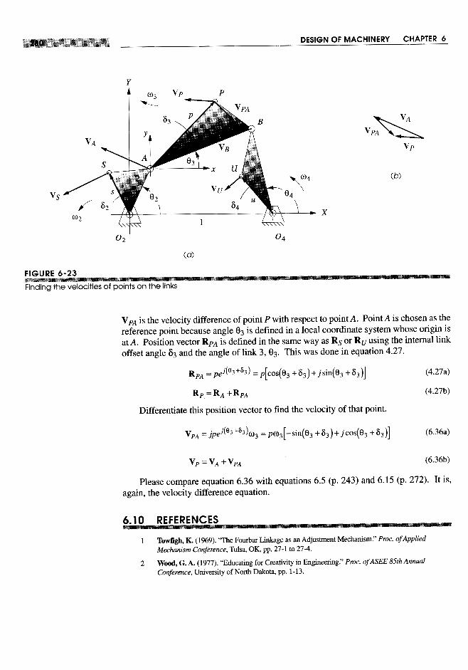


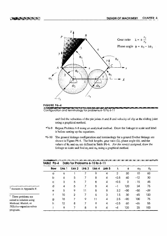


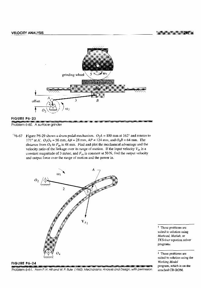
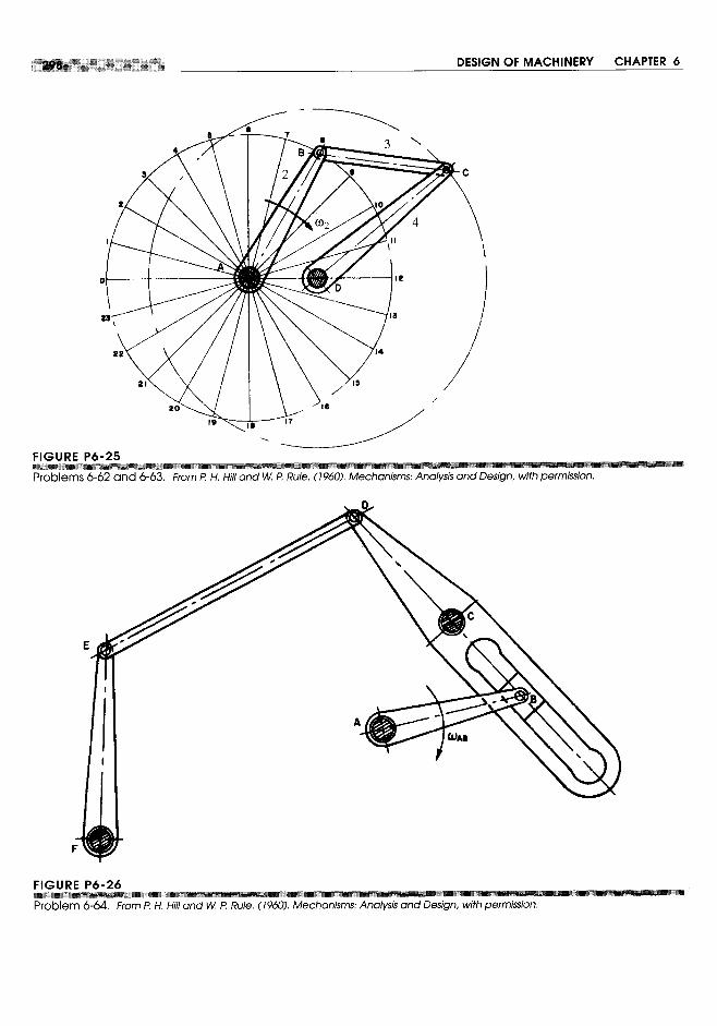
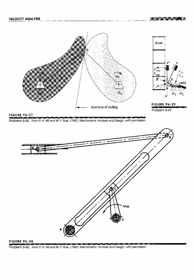


The graphical solution to this equation is shown in Figure 7-3b.
As we did for velocity analysis, we give these two cases different names despite thefact that the same equation applies. Repeating the definition from Section 6.1 (p. 241),modified to refer to acceleration:
CASE 1: Two points in the same body => acceleration difference
CASE 2: Two points in different bodies => relative acceleration
7.2 GRAPHICAL ACCELERATION ANALYSIS
The comments made in regard to graphical velocity analysis in Section 6.2 (p. 244) applyas well to graphical acceleration analysis. Historically, graphical methods were the onlypractical way to solve these acceleration analysis problems. With some practice, and withproper tools such as a drafting machine or CAD package, one can fairly rapidly solve forthe accelerations of particular points in a mechanism for anyone input position by draw-ing vector diagrams. However, if accelerations for many positions of the mechanism areto be found, each new position requires a completely new set of vector diagrams be drawn.Very little of the work done to solve for the accelerations at position 1 carries over to po-sition 2, etc. This is an even more tedious process than that for graphical velocity analy-sis because there are more components to draw. Nevertheless, this method still has morethan historical value as it can provide a quick check on the results from a computer pro-


This equation represents the absolute acceleration of some general point P referenced tothe origin of the global coordinate system. The right side defines it as the sum of the ab-solute acceleration of some other reference point A in the same system and the accelera-tion difference (or relative acceleration) of point P versus pointA. These terms are thenfurther broken down into their normal (centripetal) and tangential components which havedefinitions as shown in equation 7.2 (p. 301).
Let us review what was done in Example 7-1 in order to extract the general strategyfor solution of this class of problem. We started at the input side of the mechanism, asthat is where the driving angular acceleration cx2 was defined. We first looked for a point(A) for which the motion was pure rotation. We then solved for the absolute accelerationof that point (AA) using equations 7.4 and 7.6 by breaking AA into its normal and tangen-tial components. (Steps 1and 2)
We then used the point (A) just solved for as a reference point to define the transla-tion component in equation 7.4 written for a new point (B). Note that we needed to choosea second point (B) which was in the same rigid body as the reference point (A) which wehad already solved, and about which we could predict some aspect of the new point's(B's) acceleration components. In this example, we knew the direction of the componentA~, though we did not yet know its magnitude. We could also calculate both magnitude


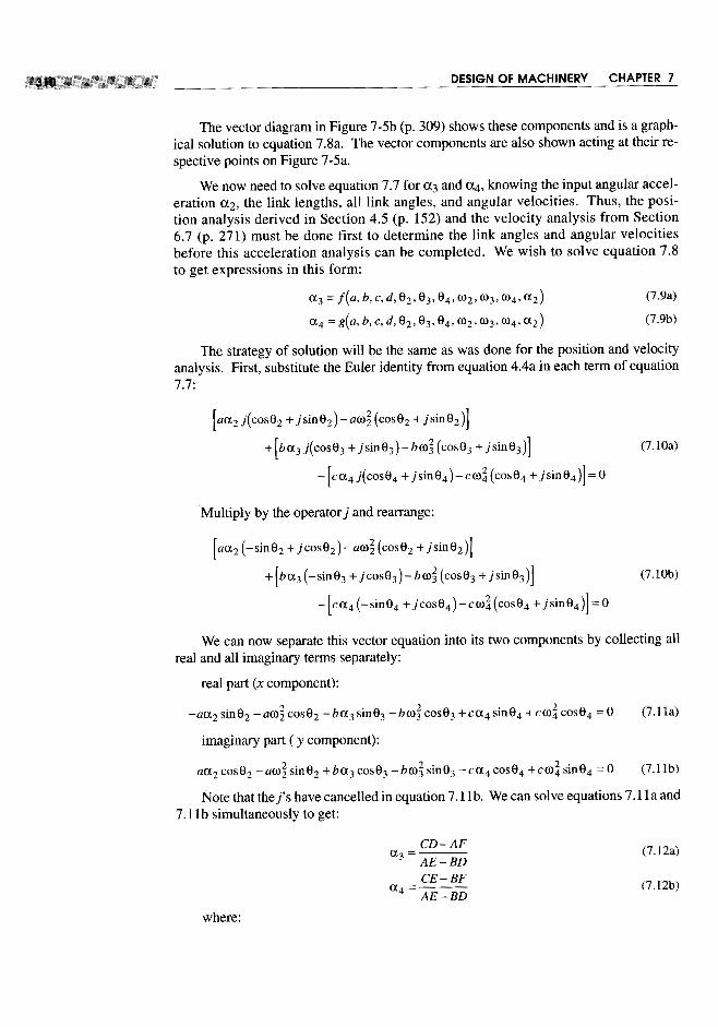
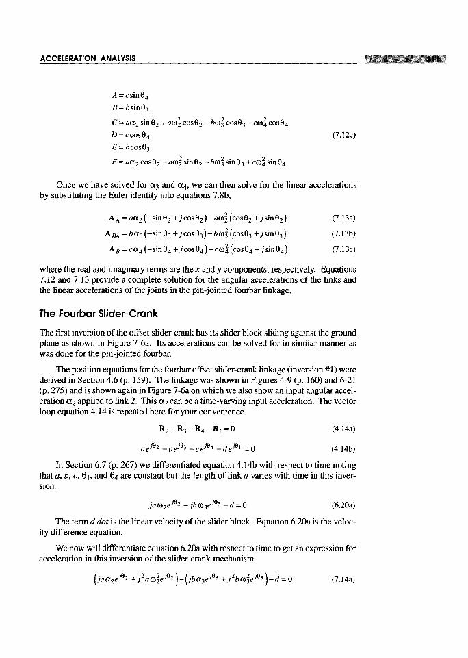


depending on the sense of 0). (Note that we chose to align the position vector Rp with theaxis of slip in Figure 7-7 which can always be done regardless of the location of the cen-ter of rotation-also see Figure 7-6 (p. 312) where RJ is aligned with the axis of slip.) Allfour components from equation 7.19 are shown acting on point P in Figure 7-7b. The totalacceleration Ap is the vector sum of the four terms as shown in Figure 7-7c. Note thatthe normal acceleration term in equation 7.19b is negative in sign, so it becomes a sub-traction when substituted in equation 7.19c.
This Coriolis component of acceleration will always be present when there is a ve-locity of slip associated with any member which also has an angular velocity. In theabsence of either of those two factors the Coriolis component will be zero. You have prob-ably experienced Coriolis acceleration if you have ever ridden on a carousel or merry-go-round. If you attempted to walk radially from the outside to the inside (or vice versa)while the carousel was turning, you were thrown sideways by the inertial force due to theCoriolis acceleration. You were the slider block in Figure 7-7, and your slip velocity com-bined with the rotation of the carousel created the Coriolis component. As you walkedfrom a large radius to a smaller one, your tangential velocity had to change to match thatof the new location of your foot on the spinning carousel. Any change in velocity re-quires an acceleration to accomplish. It was the "ghost of Coriolis" that pushed you side-ways on that carousel.
Another example of the Coriolis component is its effect on weather systems. Largeobjects which exist in the earth's lower atmosphere, such as hurricanes, span enough areato be subject to significantly different velocities at their northern and southern extremi-ties. The atmosphere turns with the earth. The earth's surface tangential velocity due toits angular velocity varies from zero at the poles to a maximum of about 1000 mph at theequator. The winds of a storm system are attracted toward the low pressure at its center.These winds have a slip velocity with respect to the surface, which in combination withthe earth's 0), creates a Coriolis component of acceleration on the moving air masses. ThisCoriolis acceleration causes the inrushing air to rotate about the center, or "eye" of thestorm system. This rotation will be counterclockwise in the northei-n hemisphere andclockwise in the southern hemisphere. The movement of the entire storm system fromsouth to north also creates a Coriolis component which will tend to deviate the storm'strack eastward, though this effect is often overridden by the forces due to other large airmasses such as high-pressure systems which can deflect a storm. These complicated fac-tors make it difficult to predict a large storm's true track.
Note that in the analytical solution presented here, the Coriolis component will be ac-counted for automatically as long as the differentiations are correctly done. However,when doing a graphical acceleration analysis one must be on the alert to recognize thepresence of this component, calculate it, and include it in the vector diagrams when itstwo constituents Vslip and 0) are both nonzero.
The Fourbar Inverted Slider-Crank
The position equations for the fourbar inverted slider-crank linkage were derived in Sec-tion 4.7 (p. 159). The linkage was shown in Figures 4-10 (p. 162) and 6-22 (p. 277) andis shown again in Figure 7-8a on which we also show an input angular acceleration a2applied to link 2. This a2 can vary with time. The vector loop equations 4.14 (p. 311) arevalid for this linkage as well.


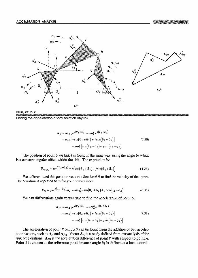

Please compare equation 7.32 with equation 7.4 (p. 302). It is again the accelera-tion difference equation. Note that this equation applies to any point on any link at anyposition for which the positions and velocities are defined. It is a general solution forany rigid body.
7.6 HUMAN TOLERANCE OF ACCELERATION
It is interesting to note that the human body does not sense velocity, except with the eyes,but is very sensitive to acceleration. Riding in an automobile, in the daylight, one cansee the scenery passing by and have a sense of motion. But, traveling at night in a com-mercial airliner at a 500 mph constant velocity, we have no sensation of motion as longas the flight is smooth. What we will sense in this situation is any change in velocity dueto atmospheric turbulence, takeoffs, or landings. The semicircular canals in the inner earare sensitive accelerometers which report to us on any accelerations which we experi-ence. You have no doubt also experienced the sensation of acceleration when ridingin an elevator and starting, stopping, or turning in an automobile. Accelerations pro-duce dynamic forces on physical systems, as expressed in Newton's second law,F=ma. Force is proportional to acceleration, for a constant mass. The dynamic forcesproduced within the human body in response to acceleration can be harmful if excessive.

The human body is, after all, not rigid. It is a loosely coupled bag of water and tissue,most of which is quite internally mobile. Accelerations in the headward or footward direc-tions will tend to either starve or flood the brain with blood as this liquid responds to New-ton's law and effectively moves within the body in a direction opposite to the imposed accel-eration as it lags the motion of the skeleton. Lack of blood supply to the brain causes black-out; excess blood supply causes redout. Either results in death if sustained for a long enoughperiod.
A great deal of research has been done, largely by the military and NASA, to deter-mine the limits of human tolerance to sustained accelerations in various directions. Fig-ure 7-10 shows data developed from such tests. [1] The units of linear acceleration weredefined in Table 1-4 (p. 19) as inlsec2, ft/sec2, or m/sec2. Another common unit for ac-celeration is the g, defined as the acceleration due to gravity, which on Earth at sea level isapproximately 386 inlsec2, 32.2 ftJsec2, or 9.8 m/sec2. The g is a very convenient unit touse for accelerations involving the human as we live in a 1 g environment. Our weight,felt on our feet or buttocks, is defined by our mass times the acceleration due to gravityor mg. Thus an imposed acceleration of 1 g above the baseline of our gravity, or 2 g's,will be felt as a doubling of our weight. At 6 g's we would feel six times as heavy asnormal and would have great difficulty even moving our arms against that acceleration.Figure 7-10 shows that the body's tolerance of acceleration is a function of its directionversus the body, its magnitude, and its duration. Note also that the data used for this chartwere developed from tests on young, healthy military personnel in prime physical con-dition. The general population, children and elderly in particular, should not be expectedto be able to withstand such high levels of acceleration. Since much machinery is de-signed for human use, these acceleration tolerance data should be of great interest andvalue to the machine designer. Several references dealing with these human factors dataare provided in the bibliography to Chapter 1 (p. 20).
Another useful benchmark when designing machinery for human occupation is toattempt to relate the magnitudes of accelerations which you commonly experience to thecalculated values for your potential design. Table 7-1 lists some approximate levels ofacceleration, in g's, which humans can experience in everyday life. Your own experienceof these will help you develop a "feel" for the values of acceleration which you encounterin designing machinery intended for human occupation.
Note that machinery which does not carry humans is limited in its acceleration lev-els only by considerations of the stresses in its parts. These stresses are often generatedin large part by the dynamic forces due to accelerations. The range of acceleration valuesin such machinery is so wide that it is not possible to comprehensively define any guide-lines for the designer as to acceptable or unacceptable levels of acceleration. If the mov-ing mass is small, then very large numerical values of acceleration are reasonable. If themass is large, the dynamic stresses which the materials can sustain may limit the allow-able accelerations to low values. Unfortunately, the designer does not usually know howmuch acceleration is too much in a design until completing it to the point of calculatingstresses in the parts. This usually requires a fairly complete and detailed design. If thestresses turn out to be too high and are due to dynamic forces, then the only recourse isto iterate back through the design process and reduce the accelerations and or masses inthe design. This is one reason that the design process is a circular and not a linear one.

As one point of reference, the acceleration of the piston in a small, four-cylindereconomy car engine (about 1.5L displacement) at idle speed is about 40 g's. At highwayspeeds the piston acceleration may be as high as 700 g's. At the engine's top speed of6000 rpm the peak piston acceleration is 2000 g's! As long as you're not riding on thepiston, this is acceptable. These engines last a long time in spite of the high accelerationsthey experience. One key factor is the choice of low-mass, high-strength materials forthe moving parts to both keep the dynamic forces down at these high accelerations andto enable them to tolerate high stresses.
7.7 JERK
No, not you! The time derivative of acceleration is called jerk, pulse, or shock. Thename is apt, as it conjures the proper image of this phenomenon. Jerk is the time rate ofchange of acceleration. Force is proportional to acceleration. Rapidly changing accel-eration means a rapidly changing force. Rapidly changing forces tend to "jerk" the ob-ject about! You have probably experienced this phenomenon when riding in an automo-bile. If the driver is inclined to 'jackrabbit" starts and accelerates violently away fromthe traffic light, you will suffer from large jerk because your acceleration will go from zeroto a large value quite suddenly. But, when Jeeves, the chauffeur, is driving the Rolls, healways attempts to minimize jerk by accelerating gently and smoothly, so that Madameis entirely unaware of the change.


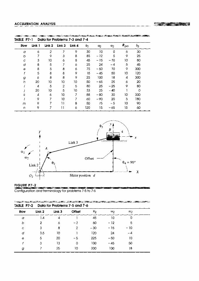
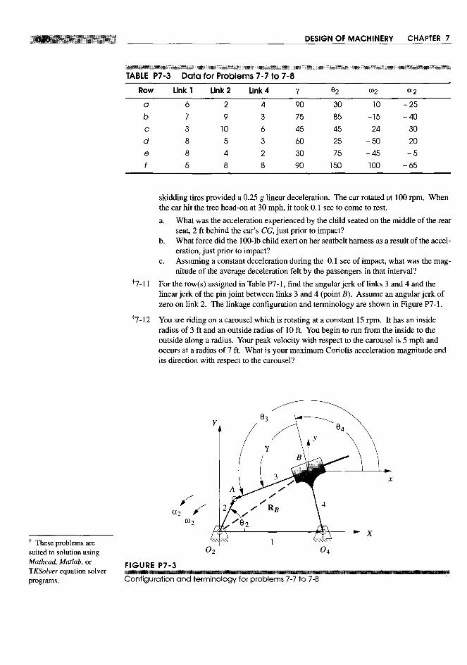


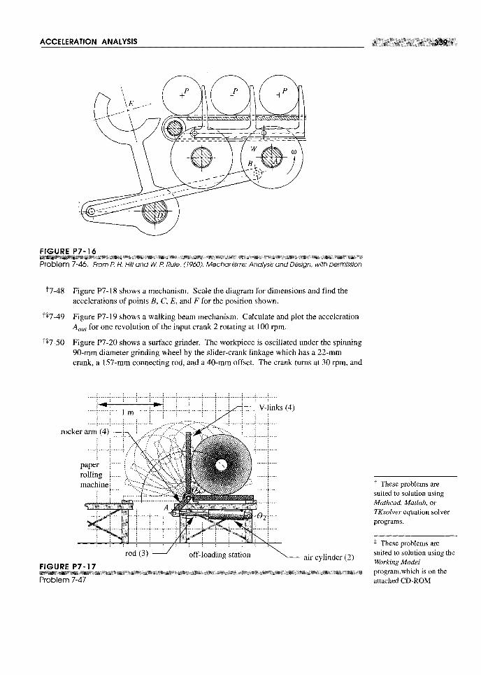


8.0 INTRODUCTION
Cam-follower systems are frequently used in all kinds of machines. The valves in yourautomobile engine are opened by cams. Machines used in the manufacture of many con-sumer goods are full of cams. Compared to linkages, cams are easier to design to give aspecific output function, but they are much more difficult and expensive to make than alinkage. Cams are a form of degenerate fourbar linkage in which the coupler link hasbeen replaced by a half joint as shown in Figure 8-1. This topic was discussed in Sec-tion 2.9 (p. 40) on linkage transformation (see also Figure 2-10, p. 41). For anyone in-stantaneous position of earn and follower, we can substitute an effective linkage whichwill, for that instantaneous position, have the same motion as the original. In effect, theearn-follower is a fourbar linkage with variable-length (effective) links. It is this con-ceptual difference that makes the earn-follower such a flexible and useful function gen-erator. We can specify virtually any output function we desire and quite likely create acurved surface on the earn to generate that function in the motion of the follower. Weare not limited to fixed-length links as we were in linkage synthesis. The earn-followeris an extremely useful mechanical device, without which the machine designer's taskswould be more difficult to accomplish. But, as with everything else in engineering, thereare trade-offs. These will be discussed in later sections. A list of the variables used inthis chapter is provided in Table 8-1.
This chapter will present the proper approach to designing a earn-follower system,and in the process also present some less than proper designs as examples of the prob-lems which inexperienced earn designers often get into. Theoretical considerations ofthe mathematical functions commonly used for earn curves will be discussed. Methodsfor the derivation of custom polynomial functions, to suit any set of boundary conditions,will be presented. The task of sizing the earn with considerations of pressure angle andradius of curvature will be addressed, and manufacturing processes and their limitations

discussed. The computer program DYNACAM will be used throughout the chapter as atool to present and illustrate design concepts and solutions. A user manual for this pro-gram is in Appendix A. The reader can refer to that section at any time without loss ofcontinuity in order to become familiar with the program's operation.
8.1 CAM TERMINOLOGY
Cam-follower systems can be classified in several ways: by type of follower motion,either translating or rotating (oscillating); by type of earn, radial, cylindrical, three-di-mensional; by type of joint closure, either force- or fonn-closed; by type of follower,curved or flat, rolling or sliding; by type of motion constraints, critical extreme posi-tion (CEP), critical path motion (CPM); by type of motion program, rise-fall (RF),rise-fall-dwell (RFD), rise-dwell-fall-dwell (RDFD). We will now discuss each of theseclassification schemes in more detail.

Type of Follower Motion
Figure 8-1a shows a system with an oscillating, or rotating, follower. Figure 8-1b showsa translating follower. These are analogous to the crank-rocker fourbar and the slider-crank fourbar linkages, respectively. An effective fourbar linkage can be substituted forthe earn-follower system for any instantaneous position. The lengths of the effectivelinks are determined by the instantaneous locations of the centers of curvature of earnand follower as shown in Figure 8-1. The velocities and accelerations of the earn-fol-lower system can be found by analyzing the behavior of the effective linkage for anyposition. A proof of this can be found in reference [1]. Of course, the effective linkschange length as the earn-follower moves giving it an advantage over a pure linkage asthis allows more flexibility in meeting the desired motion constraints.

The choice between these two forms of the earn-follower is usually dictated by thetype of output motion desired. If true rectilinear translation is required, then the trans-lating follower is dictated. If pure rotation output is needed, then the oscillator is theobvious choice. There are advantages to each of these approaches, separate from theirmotion characteristics, depending on the type of follower chosen. These will be dis-cussed in a later section.
Type of Joint Closure
Force and form closure were discussed in Section 2.3 (p. 24) on the subject of jointsand have the same meaning here. Force closure, as shown in Figure 8-1 (p. 347), re-quires an external force be applied to the joint in order to keep the two links, cam andfollower, physically in contact. This force is usually provided by a spring. This force,defined as positive in a direction which closes the joint, cannot be allowed to becomenegative. If it does, the links have lost contact because aforce-closed joint can only push,not pull. Form closure, as shown in Figure 8-2, closes the joint by geometry. No exter-nal force is required. There are really two earn surfaces in this arrangement, one surfaceon each side of the follower. Each surface pushes, in its turn, to drive the follower inboth directions.
Figure 8-2a and b shows track or groove cams which capture a single follower inthe groove and both push and pull on the follower. Figure 8-2c shows another variety ofform-closed earn-follower arrangement, called conjugate cams. There are two camsfixed on a common shaft which are mathematical conjugates of one another. Two rollerfollowers, attached to a common arm, are each pushed in opposite directions by the con-jugate cams. When form-closed cams are used in automobile or motorcycle engine valvetrains, they are called desmodromic cams. There are advantages and disadvantages toboth force- and form-closed arrangements which will be discussed in a later section.
Type of Follower
Follower, in this context, refers only to that part of the follower link which contacts theearn. Figure 8-3 shows three common arrangements, flat-faced, mushroom (curved),and roller. The roller follower has the advantage of lower (rolling) friction than the slid-ing contact of the other two but can be more expensive. Flat-faced followers can pack-age smaller than roller followers for some earn designs and are often favored for thatreason as well as cost for automotive valve trains. Roller followers are more frequentlyused in production machinery where their ease of replacement and availability from bear-ing manufacturers' stock in any quantities are advantages. Grooved or track cams requireroller followers. Roller followers are essentially ball or roller bearings with customizedmounting details. Figure 8-5a shows two common types of commercial roller follow-ers. Flat-faced or mushroom followers are usually custom designed and manufacturedfor each application. For high-volume applications such as automobile engines, thequantities are high enough to warrant a custom-designed follower.
Type of Cam
The direction of the follower's motion relative to the axis of rotation of the earn deter-mines whether it is a radial or axial earn. All cams shown in Figures 8-1 to 8-3 are ra-

dial cams because the follower motion is generally in a radial direction. Open radialcams are also called plate cams.
Figure 8-4 shows an axial carn whose follower moves parallel to the axis of earnrotation. This arrangement is also called a face earn if open (force-closed) and a cylin-drical or barrel earn if grooved or ribbed (form-closed).
Figure 8-5b shows a selection of cams of various types. Clockwise from the lowerleft, they are: an open (force-closed) axial or face earn; an axial grooved (track) earn(form-closed) with external gear; an open radial, or plate earn (force-closed); a ribbedaxial earn (form-closed); an axial grooved (barrel) earn.


Type of Motion Constraints
There are two general categories of motion constraint, critical extreme position (CEP;also called endpoint specification) and critical path motion (CPM). Critical extremeposition refers to the case in which the design specifications define the start and finishpositions of the follower (i.e., extreme positions) but do not specify any constraints onthe path motion between the extreme positions. This case is discussed in Sections 8.3and 8.4 and is the easier of the two to design as the designer has great freedom to choosethe cam functions which control the motion between extremes. Critical path motion isa more constrained problem than CEP because the path motion, and/or one or more ofits derivatives are defined over all or part of the interval of motion. This is analogous tofunction generation in the linkage design case except that with a cam we can achieve acontinuous output function for the follower. Section 8.6 discusses this CPM case. It mayonly be possible to create an approximation of the specified function and still maintainsuitable dynamic behavior.
Type of Motion Program
The motion programs rise-fall (RF), rise-fall-dwell (RFD), and rise-dwell-fall-dwell(RDFD) all refer mainly to the CEP case of motion constraint and in effect define howmany dwells are present in the full cycle of motion, either none (RF), one (RFD), or more

than one (RDFD). Dwells, defined as no output motion for a specified period of inputmotion, are an important feature of cam-follower systems because it is very easy to cre-ate exact dwells in these mechanisms. The cam-follower is the design type of choicewhenever a dwell is required. We saw in Section 3.9 (p. 125) how to design dwell link-ages and found that at best we could obtain only an approximate dwell. The resultingsingle- or double-dwell linkages tend to be quite large for their output motion and aresomewhat difficult to design. (See program SIXBARfor some built-in examples of thesedwell linkages.) Cam-follower systems tend to be more compact than linkages for thesame output motion.
If your need is for a rise-fall (RF) CEP motion, with no dwell, then you should real-ly be considering a crank-rocker linkage rather than a cam-follower to obtain all the link-age's advantages over cams of reliability, ease of construction, and lower cost whichwere discussed in Section 2.15 (p. 55). If your needs for compactness outweigh thoseconsiderations, then the choice of a cam-follower in the RF case may be justified. Also,if you have a CPM design specification, and the motion or its derivatives are defined overthe interval, then a cam-follower system is the logical choice in the RF case.
The rise-faIl-dwell (RFD) and rise-dwell-fall-dwell (RDFD) cases are obviouschoices for cam- followers for the reasons discussed above. However, each of these twocases has its own set of constraints on the behavior of the cam functions at the interfacesbetween the segments which control the rise, the fall, and the dwells. In general, we mustmatch the boundary conditions (BCs) of the functions and their derivatives at all inter-faces between the segments of the carn. This topic will be thoroughly discussed in thefollowing sections.
8.2 S V A J DIAGRAMS
The first task faced by the cam designer is to select the mathematical functions to be usedto define the motion of the follower. The easiest approach to this process is to "linear-ize" the cam, i.e., "unwrap it" from its circular shape and consider it as a function plot-ted on cartesian axes. We plot the displacement function s, its first derivative velocity v,its second derivative acceleration a, and its third derivative jerk}, all on aligned axes asa function of camshaft angle e as shown in Figure 8-6. Note that we can consider theindependent variable in these plots to be either time t or shaft angle e, as we know theconstant angular velocity (J) of the camshaft and can easily convert from angle to time andvice versa.
e = rot (8.1)
Figure 8-6a shows the specifications for a four-dwell cam that has eight segments,RDFDRDFD. Figure 8-6b shows the s v a} curves for the whole cam over 360 degreesof camshaft rotation. A cam design begins with a definition of the required cam func-tions and their s va} diagrams. Functions for the nondwell cam segments should be cho-sen based on their velocity, acceleration, and jerk characteristics and the relationships atthe interfaces between adjacent segments including the dwells. These function charac-teristics can be conveniently and quickly investigated with program DYNACAMwhichgenerated the data and plots shown in Figure 8-6.

8.3 DOUBLE-DWELLCAM DESIGN-CHOOSING 5 VA JFUNCTIONS
Many cam design applications require multiple dwells. The double-dwell case is quitecommon. Perhaps a double-dwell cam is driving a part feeding station on a productionmachine that makes toothpaste. This hypothetical cam's follower is fed an empty tooth-paste tube (during the low dwell), then moves the empty tube into a loading station (dur-ing the rise), holds the tube absolutely still in a critical extreme position (CEP) whiletoothpaste is squirted into the open bottom of the tube (during the high dwell), and thenretracts the filled tube back to the starting (zero) position and holds it in this other criti-cal extreme position. At this point, another mechanism (during the low dwell) picks thetube up and carries it to the next operation, which might be to seal the bottom of the tube.A similar cam could be used to feed, align, and retract the tube at the bottom-sealing sta-tion as well.
Cam specifications such as this are often depicted on a timing diagram as shown inFigure 8-7 which is a graphical representation of the specified events in the machinecycle. A machine's cycle is defined as one revolution of its master driveshaft. In a com-plicated machine, such as our toothpaste maker, there will be a timing diagram for eachsubassembly in the machine. The time relationships among all subassemblies are definedby their timing diagrams which are all drawn on a common time axis. Obviously allthese operations must be kept in precise synchrony and time phase for the machine towork.

Solution:
I The naive or inexperienced cam designer might proceed with a design as shown in Figure8-8a. Taking the given specifications literally, it is tempting to merely "connect the dots" onthe timing diagram to create the displacement (s) diagram. (After all, when we wrap this sdiagram around a circle to create the actual cam, it will look quite smooth despite the sharpcorners on the s diagram.) The mistake our beginning designer is making here is to ignorethe effect on the higher derivatives of the displacement function which results from this sim-plistic approach.
2 Figure 8-8b, c, and d shows the problem. Note that we have to treat each segment of the cam(rise, fall, dwell) as a separate entity in developing mathematical functions for the cam. Tak-ing the rise segment (#2) first, the displacement function in Figure 8-8a during this portionis a straight line, or first-degree polynomial. The general equation for a straight line is:
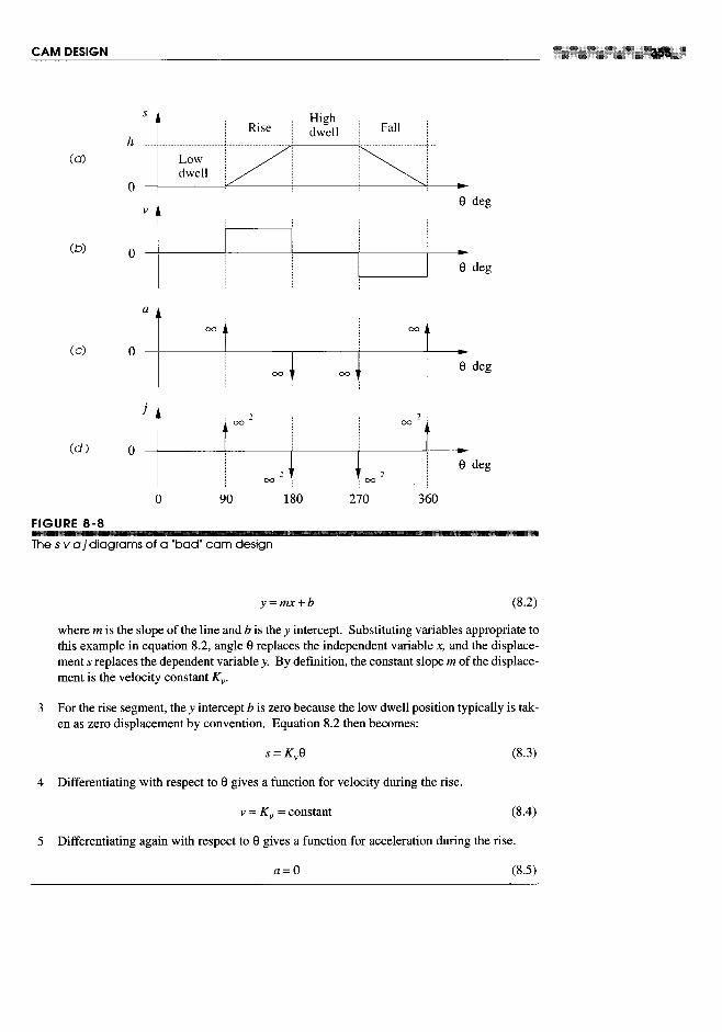

This seems too good to be true (and it is). Zero acceleration means zero dynamicforce. This cam appears to have no dynamic forces or stresses in it!
Figure 8-8 shows what is really happening here. If we return to the displacementfunction and graphically differentiate it twice, we will observe that, from the definitionof the derivative as the instantaneous slope ofthe function, the acceleration is in fact zeroduring the interval. But, at the boundaries of the interval, where rise meets low dwellon one side and high dwell on the other, note that the velocity function is multivalued.There are discontinuities at these boundaries. The effect of these discontinuities is tocreate a portion of the velocity curve which has infinite slope and zero duration. Thisresults in the infinite spikes of acceleration shown at those points.
These spikes are more properly called Dirac delta functions. Infinite accelerationcannot really be obtained, as it requires infinite force. Clearly the dynamic forces willbe very large at these boundaries and will create high stresses and rapid wear. In fact, ifthis carn were built and run at any significant speeds, the sharp comers on the displace-ment diagram which are creating these theoretical infinite accelerations would be quick-ly worn to a smoother contour by the unsustainable stresses generated in the materials.This is an unacceptable design.
The unacceptability of this design is reinforced by the jerk diagram which showstheoretical values of infinity squared at the discontinuities. The problem has been en-gendered by an inappropriate choice of displacement function. In fact, the cam designershould not be as concerned with the displacement function as with its higher derivatives.
The Fundamental law of Cam Design
Any cam designed for operation at other than very low speeds must be designed with thefollowing constraints:
The cam function must be continuous through the first and second derivatives of dis-placement across the entire interval (360 degrees).
corollary:
The jerk function must be finite across the entire interval (360 degrees).
In any but the simplest of carns, the cam motion program cannot be defined by asingle mathematical expression, but rather must be defined by several separate functions,each of which defines the follower behavior over one segment, or piece, of the carn.These expressions are sometimes called piecewise functions. These functions must havethird-order continuity (the function plus two derivatives) at all boundaries. The dis-placement, velocity and acceleration functions must have no discontinuities inthem. *
If any discontinuities exist in the acceleration function, then there will be infinitespikes, or Dirac delta functions, appearing in the derivative of acceleration, jerk. Thusthe corollary merely restates the fundamental law of cam design. Our naive designerfailed to recognize that by starting with a low-degree (linear) polynomial as the displace-ment function, discontinuities would appear in the upper derivatives.
Polynomial functions are one of the best choices for carns as we shall shortly see-,but they do have one fault that can lead to trouble in this application. Each time they are
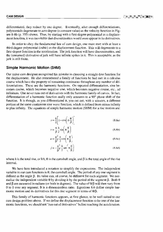

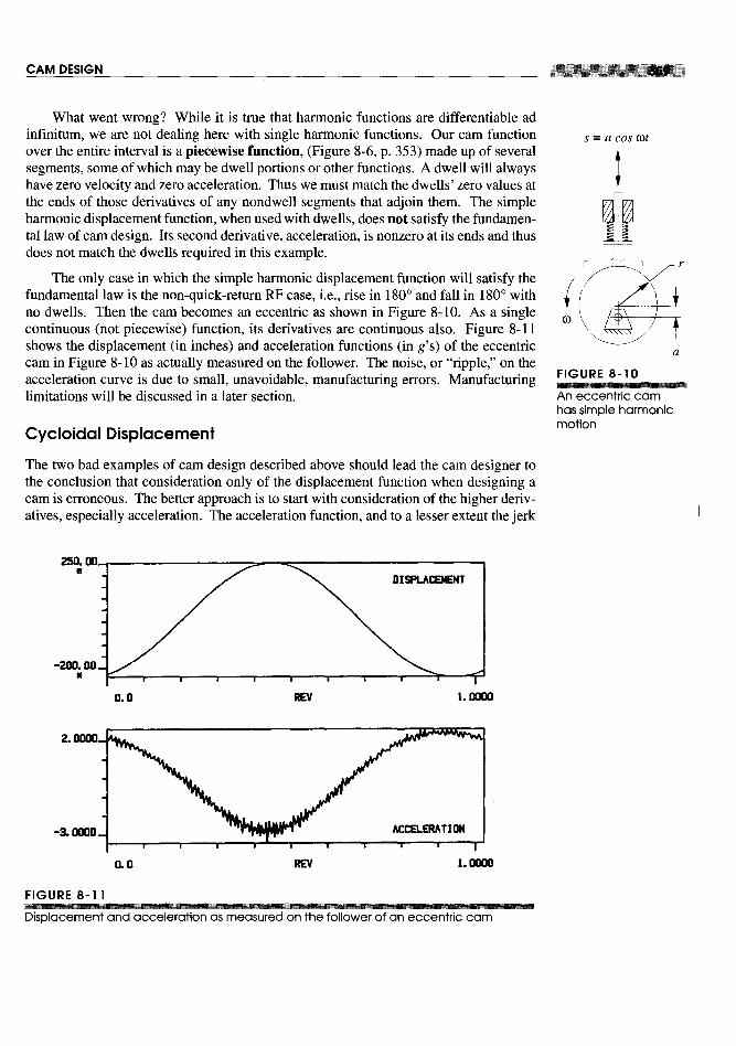


Figure 8-22 shows the displacement curves for these three earn programs. (Openthe diskfile E08-04.cam in program DYNACAM also.) Note how little difference there isbetween the displacement curves despite the large differences in their acceleration wave-forms in Figure 8-18. This is evidence of the smoothing effect of the integration pro-cess. Differentiating any two functions will exaggerate their differences. Integrationtends to mask their differences. It is nearly impossible to recognize these very different-ly behaving earn functions by looking only at their displacement curves. This is furtherevidence of the folly of our earlier naive approach to earn design which dealt exclusive-ly with the displacement function. The earn designer must be concerned with the higherderivatives of displacement. The displacement function is primarily of value to the man-ufacturer of the earn who needs its coordinate information in order to cut the earn.
FALL FUNCTIONS We have used only the rise portion of the earn for these exam-ples. The fall is handled similarly. The rise functions presented here are applicable tothe fall with slight modification. To convert rise equations to fall equations, it is onlynecessary to subtract the rise displacement function s from the maximum lift h and tonegate the higher derivatives, v, a, and}.
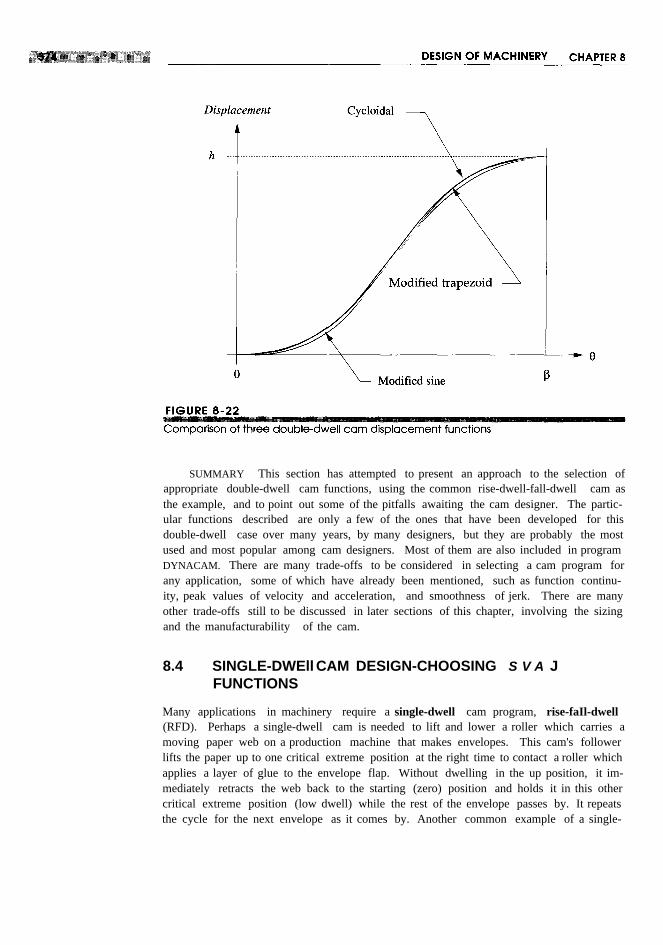
SUMMARY This section has attempted to present an approach to the selection ofappropriate double-dwell cam functions, using the common rise-dwell-fall-dwell cam asthe example, and to point out some of the pitfalls awaiting the cam designer. The partic-ular functions described are only a few of the ones that have been developed for thisdouble-dwell case over many years, by many designers, but they are probably the mostused and most popular among cam designers. Most of them are also included in programDYNACAM. There are many trade-offs to be considered in selecting a cam program forany application, some of which have already been mentioned, such as function continu-ity, peak values of velocity and acceleration, and smoothness of jerk. There are manyother trade-offs still to be discussed in later sections of this chapter, involving the sizingand the manufacturability of the cam.
8.4 SINGLE-DWEllCAM DESIGN-CHOOSING S V A JFUNCTIONS
Many applications in machinery require a single-dwell cam program, rise-faIl-dwell(RFD). Perhaps a single-dwell cam is needed to lift and lower a roller which carries amoving paper web on a production machine that makes envelopes. This cam's followerlifts the paper up to one critical extreme position at the right time to contact a roller whichapplies a layer of glue to the envelope flap. Without dwelling in the up position, it im-mediately retracts the web back to the starting (zero) position and holds it in this othercritical extreme position (low dwell) while the rest of the envelope passes by. It repeatsthe cycle for the next envelope as it comes by. Another common example of a single-

Solution:
I Figure 8-23 shows a cycloidal displacement rise and separate cycloidal displacement fall ap-plied to this single-dwell example. Note that the displacement (s) diagram looks acceptablein that it moves the followerfrom the low to thehigh positionand back in the requiredintervals.
2 The velocity (v) also looks acceptable in shape in that it takes the follower from zero veloc-ity at the low dwell to a peak value of 19.1 in/sec (0.49 rn/sec) to zero again at the maximumdisplacement, where the glue is applied.
3 Figure 8-23 shows the acceleration function for this solution. Its maximum absolute valueis about 573 in/sec2.
4 The problem is that this acceleration curve has an unnecessary return to zero at the end ofthe rise. It is unnecessary because the acceleration during the first part of the fall is also neg-ative. It would be better to keep it in the negative region at the end of the rise.
5 This unnecessary oscillation to zero in the acceleration causes the jerk to have more abruptchanges and discontinuities. The only real justification for taking the acceleration to zero isthe need to change its sign (as is the case halfway through the rise or fall) or to match an ad-jacent segment which has zero acceleration.
The reader may input the file E08-0S.cam to program DYNACAMto investigate thisexample in more detail.
For the single-dwell case we would like a function for the rise which does not returnits acceleration to zero at the end of the interval. The function for the fall should beginwith the same nonzero acceleration value as ended the rise and then be zero at its termi-I1US to match the dwell. One function which meets those criteria is the double harmon-ic which gets its name from its two cosine terms, one of which is a half-period harmonicmd the other a full-period wave. The equations for the double harmonic functions are:

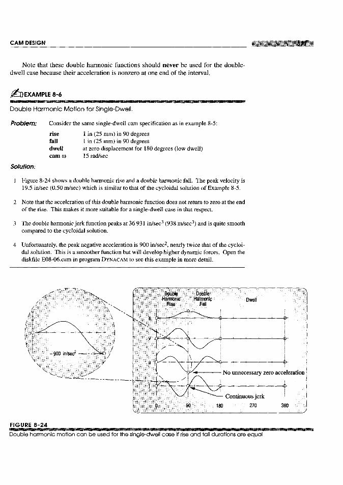


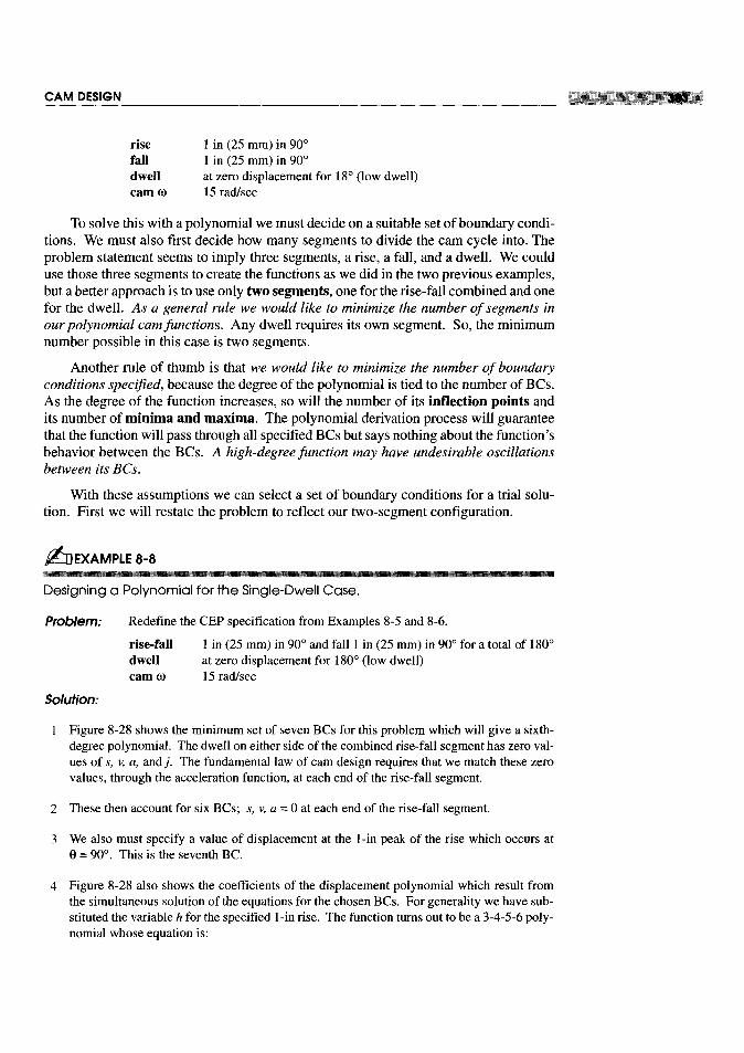

SUMMARY This section has presented polynomial functions as the most versatileapproach of those shown to virtually any cam design problems. It is only since the de-velopment and general availability of computers that these functions have become prac-tical to use, as the computation to solve the simultaneous equations is often beyond handcalculation abilities. With the availability of a design aid to solve the equations such asprogram DYNACAM, polynomials have become a practical and preferable way to solvemany cam design problems. Spline functions, of which polynomials are a subset, offereven more flexibility in meeting boundary constraints and other cam performance crite-ria)5] [7] Space does not permit a detailed exposition of spline functions as applied tocam systems here. See the references for more information.

8.6 CRITICAL PATH MOTION (CPM)
Probably the most common application of critical path motion (CPM) specifications inproduction machinery design is the need for constant velocity motion. There are twogeneral types of automated production machinery in common use, intermittent motionassembly machines and continuous motion assembly machines.
Intermittent motion assembly machines carry the manufactured goods from workstation to work station, stopping the workpiece or subassembly at each station whileanother operation is performed upon it. The throughput speed of this type of automatedproduction machine is typically limited by the dynamic forces which are due to acceler-ations and decelerations of the mass of the moving parts of the machine and its work-pieces. The workpiece motion may be either in a straight line as on a conveyor or in acircle as on a rotary table as shown in Figure 8-21 (p.372).
Continuous motion assembly machines never allow the workpiece to stop andthus are capable of higher throughput speeds. All operations are performed on a movingtarget. Any tools which operate on the product have to "chase" the moving assembly lineto do their job. Since the assembly line (often a conveyor belt or chain, or a rotary table)is moving at some constant velocity, there is a need for mechanisms to provide constantvelocity motion, matched exactly to the conveyor, in order to carry the tools alongsidefor a long enough time to do their job. These cam driven "chaser" mechanisms must thenreturn the tool quickly to its start position in time to meet the next part or subassemblyon the conveyor (quick-return). There is a motivation in manufacturing to convert fromintermittent motion machines to continuous motion in order to increase production rates.Thus there is considerable demand for this type of constant velocity mechanism. Theearn-follower system is well suited to this problem, and the polynomial earn function isparticularly adaptable to the task.
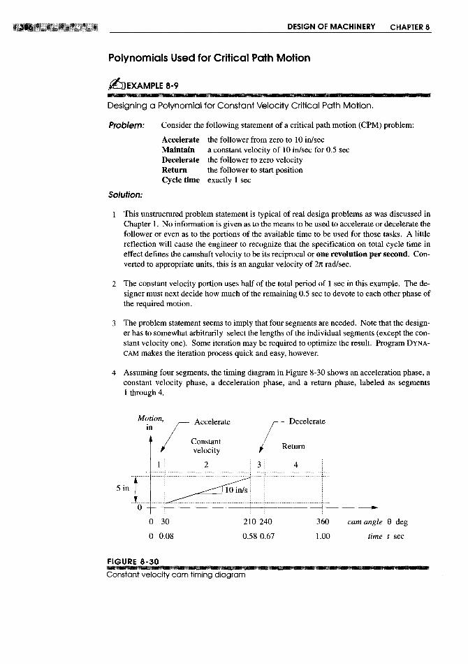


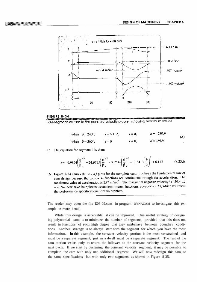
The reader may open the file E08-09.cam in program DYNACAM to investigate this ex-ample in more detail.
While this design is acceptable, it can be improved. One useful strategy in design-ing polynomial cams is to minimize the number of segments, provided that this does notresult in functions of such high degree that they misbehave between boundary condi-tions. Another strategy is to always start with the segment for which you have the mostinformation. In this example, the constant velocity portion is the most constrained andmust be a separate segment, just as a dwell must be a separate segment. The rest of thecam motion exists only to return the follower to the constant velocity segment for thenext cycle. If we start by designing the constant velocity segment, it may be possible tocomplete the cam with only one additional segment. We will now redesign this cam, tothe same specifications but with only two segments as shown in Figure 8-35.


For a fall instead of a rise, subtract the rise displacement expressions from the totalrise L and negate all the higher derivatives.
To fit these functions to a particular constant velocity situation, solve either equa-tion 8.25b or 8.26b (depending on which function is desired) for the value of L whichresults from the specification of the known constant velocity v to be matched at e = ~ ore = O. You will have to choose a value of ~ for the interval of this half-cycloid which isappropriate to the problem. In our example above, the value of ~ = 30° used for the firstsegment of the four-piece polynomial could be tried as a first iteration. Once L and ~ areknown, all the functions are defined.
The same approach can be taken with the modified sine and the simple harmonicfunctions. Either half of their full-rise functions can be sized to match with a constantvelocity segment. The half-modified sine function mated with a constant velocity seg-ment has the advantage of low peak velocity, useful with large inertia loads. Whenmatched to a constant velocity, the half simple harmonic has the same disadvantage of infi-nite jerk as its full-rise counterpart does when matched to a dwell, so it is not recommended.
We will now solve the previous constant velocity example problem using half-cyc-loid, constant velocity, and full-fall modified sine functions.


These results are nearly as low as the values from the two-segment polynomial so-lution in Example 8-10 (p. 391). The factor that makes this an inferior cam design toExample 8-10 is the unnecessary returns to zero in the acceleration waveform. This cre-ates a more "ragged" jerk function which will increase vibration problems. The polyno-mial approach is superior to the other solutions presented in this case as it often is in camdesign. The reader may open the file E08-ll.cam in program DYNACAM to investigatethis example in more detail.
8.7 SIZING THE CAM-PRESSURE ANGLE AND RADIUS OFCURVATURE
Once the s v a j functions have been defined, the next step is to size the cam. There aretwo major factors which affect cam size, the pressure angle and the radius of curva-ture. Both of these involve either the base circle radius on the cam (Rb) when usingflat-faced followers, or the prime circle radius on the cam (Rp) when using roller orcurved followers.

The base circle's and prime circle's centers are at the center of rotation of the earn.The base circle is defined as the smallest circle which can be drawn tangent to the phys-ical cam suiface as shown in Figure 8-39. All radial cams will have a base circle, re-gardless of the follower type used.
The prime circle is only applicable to cams with roller followers or radiused (mush-room) followers and is measured to the center of the follower. The prime circle is de-fined as the smallest circle which can be drawn tangent to the locus of the centerline ofthe follower as shown in Figure 8-39. The locus of the centerline of the follower is calledthe pitch curve. Cams with roller followers are in fact defined for manufacture withrespect to the pitch curve rather than with respect to the earn's physical surface. Camswith flat-faced followers must be defined for manufacture with respect to their physicalsurface, as there is no pitch curve.
The process of creating the physical earn from the s diagram can be visualized con-ceptually by imagining the s diagram to be cut out of a flexible material such as rubber.The x axis of the s diagram represents the circumference of a circle, which could be ei-ther the base circle, or the prime circle, around which we will "wrap" our "rubber" sdiagram. We are free to choose the initial length of our s diagram's x axis, though theheight of the displacement curve is fixed by the earn displacement function we have cho-sen. In effect we will choose the base or prime circle radius as a design parameter andstretch the length of the s diagram's axis to fit the circumference of the chosen circle.
Pressure Angle-Roller Followers
The pressure angle is defined as shown in Figure 8-40. It is the complement of the trans-mission angle which was defined for linkages in previous chapters and has a similarmeaning with respect to earn-follower operation. By convention, the pressure angle isused for cams, rather than the transmission angle. Force can only be transmitted from
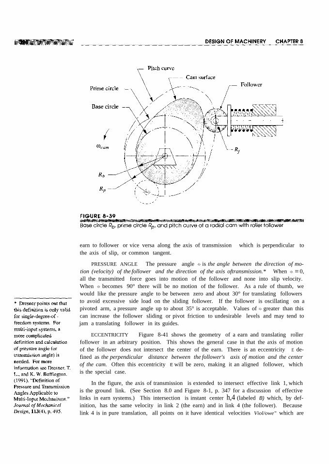
earn to follower or vice versa along the axis of transmission which is perpendicular tothe axis of slip, or common tangent.
PRESSURE ANGLE The pressure angle <\> is the angle between the direction of mo-tion (velocity) of the follower and the direction of the axis oftransmission.* When <\> = 0,all the transmitted force goes into motion of the follower and none into slip velocity.When <\> becomes 90° there will be no motion of the follower. As a rule of thumb, wewould like the pressure angle to be between zero and about 30° for translating followersto avoid excessive side load on the sliding follower. If the follower is oscillating on apivoted arm, a pressure angle up to about 35° is acceptable. Values of <\> greater than thiscan increase the follower sliding or pivot friction to undesirable levels and may tend tojam a translating follower in its guides.
ECCENTRICITY Figure 8-41 shows the geometry of a earn and translating rollerfollower in an arbitrary position. This shows the general case in that the axis of motionof the follower does not intersect the center of the earn. There is an eccentricity E de-fined as the perpendicular distance between the follower's axis of motion and the centerof the cam. Often this eccentricity E will be zero, making it an aligned follower, whichis the special case.
In the figure, the axis of transmission is extended to intersect effective link 1, whichis the ground link. (See Section 8.0 and Figure 8-1, p. 347 for a discussion of effectivelinks in earn systems.) This intersection is instant center h,4 (labeled B) which, by def-inition, has the same velocity in link 2 (the earn) and in link 4 (the follower). Becauselink 4 is in pure translation, all points on it have identical velocities Viol/owe" which are

Choosing a Prime Circle Radius
Both Rp and £ are within a transcendental expression in equation 8.29d, so they cannotbe conveniently solved for directly. The simplest approach is to assume a trial value forRp and an initial eccentricity of zero, and use program DYNACAM; your own program; oran equation solver such as Matlah, TKSolver or Mathcad to quickly calculate the valuesof <I> for the entire earn, and then adjust Rp and repeat the calculation until an acceptablearrangement is found. Figure 8-42 shows the calculated pressure angles for a four-dwellearn. Note the similarity in shape to the velocity functions for the same earn in Figure8-6 (p. 353), as that term is dominant in equation 8.29d.

USING ECCENTRICITY If a suitably small cam cannot be obtained with accept-able pressure angle, then eccentricity can be introduced to change the pressure angle.Using eccentricity to control the pressure angle has its limitations. For a positive co, apositive value of eccentricity will decrease the pressure angle on the rise but will in-crease it on the fall. Negative eccentricity does the reverse.
This is of little value with a form-closed (groove or track) carn, as it is driving thefollower in both directions. For a force-closed carn with spring return, you can some-times afford to have a larger pressure angle on the fall than on the rise because the storedenergy in the spring is attempting to speed up the camshaft on the fall, whereas the camis storing that energy in the spring on the rise. The limit of this technique can be thedegree of overspeed attained with a larger pressure angle on the fall. The resulting vari-ations in carn angular velocity may be unacceptable.

The most value gained from adding eccentricity to a follower comes in situationswhere the cam prograrn is asymmetrical and significant differences exist (with no eccen-tricity) between maximum pressure angles on rise and fall. Introducing eccentricity canbalance the pressure angles in this situation and create a smoother running cam.
If adjustments to Rp or E do not yield acceptable pressure angles, the only recourseis to return to an earlier stage in the design process and redefine the problem. Less lift ormore time to rise or fall will reduce the causes of the large pressure angle. Design is,after all, an iterative process.
Overturning Moment-Flat-Faced Follower
Figure 8-43 shows a translating, flat-faced follower running against a radial carn. Thepressure angle can be seen to be zero for all positions of cam and follower. This seemsto be giving us something for nothing, which can't be true. As the contact point movesleft and right, the point of application of the force between cam and follower moves withit. There is an overturning moment on the follower associated with this off-center forcewhich tends to jam the follower in its guides, just as did too large a pressure angle in theroller follower case. In this case, we would like to keep the carn as small as possible inorder to minimize the moment arm of the force. Eccentricity will affect the average val-ue of the moment, but the peak-to-peak variation of the moment about that average isunaffected by eccentricity. Considerations of too-large pressure angle do not limit thesize of this cam, but other factors do. The minimum radius of curvature (see below) ofthe cam surface must be kept large enough to avoid undercutting. This is true regardlessof the type of follower used.


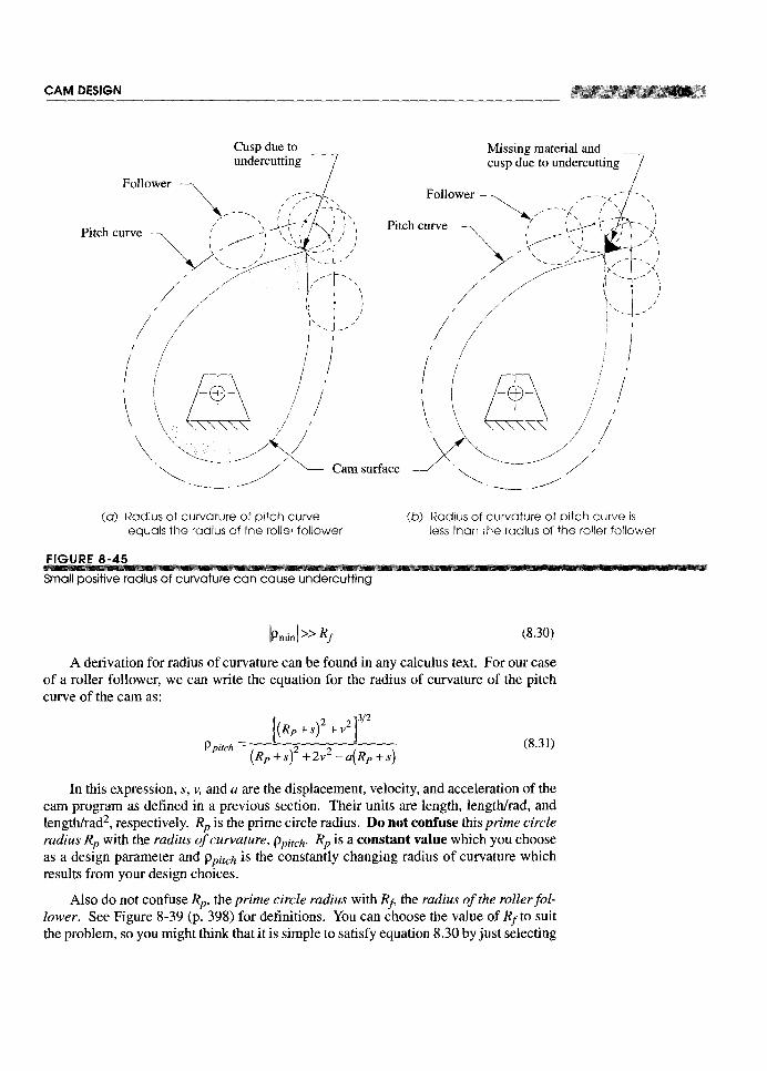


8.8 CAM MANUFACTURING CONSIDERATIONS
The preceding sections illustrate that there are a number of factors to consider when de-signing a earn. A great deal of care in design is necessary to obtain a good compromiseof all factors, some of which conflict. Once the earn design is complete a whole new setof considerations must be dealt with that involve manufacturing the earn. After all, ifyour design cannot be successfully machined in metal in a way that truly represents thetheoretical functions chosen, their benefits will not be realized. Unlike linkages, whichare very easy to make, cams are a challenge to manufacture properly.
Cams are usually made from strong, hard materials such as medium to high car-bon steels (case- or through-hardened) or cast ductile iron or grey cast iron (case-hard-ened). Cams for low loads and speeds or marine applications are sometimes made ofbrass or bronze. Even plastic cams are used in such applications as washing machinetimers where the earn is merely tripping a switch at the right time. We will concentrateon the higher load-speed situations here for which steel or cast/ductile iron are the onlypractical choices. These materials range from fairly difficult to very difficult to machinedepending on the alloy. At a minimum, a reasonably accurate milling machine is neededto make a earn. A computer controlled machining center is far preferable and is mostoften the choice for serious earn production.
Cams are typically milled with rotating cutters that in effect "tear" the metal awayleaving a less than perfectly smooth surface at a microscopic level. For a better finishand better geometric accuracy, the cam can be ground after milling away most of theunneeded material. Heat treatment is usually necessary to get sufficient hardness to pre-vent rapid wear. Steel cams are typically hardened to about Rockwell Rc 50-55. Heattreatment introduces some geometric distortion. The grinding is usually done after heat
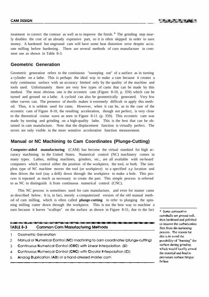
treatment to correct the contour as well as to improve the finish. * The grinding step near-ly doubles the cost of an already expensive part, so it is often skipped in order to savemoney. A hardened but unground cam will have some heat distortion error despite accu-rate milling before hardening. There are several methods of carn manufacture in com-mon use as shown in Table 8-3.
Geometric Generation
Geometric generation refers to the continuous "sweeping out" of a surface as in turninga cylinder on a lathe. This is perhaps the ideal way to make a cam because it creates atruly continuous surface with an accuracy limited only by the quality of the machine andtools used. Unfortunately there are very few types of cams that can be made by thismethod. The most obvious one is the eccentric cam (Figure 8-10, p. 359) which can beturned and ground on a lathe. A cycloid can also be geometrically generated. Very fewother curves can. The presence of dwells makes it extremely difficult to apply this meth-od. Thus, it is seldom used for cams. However, when it can be, as in the case of theeccentric cam of Figure 8-10, the resulting acceleration, though not perfect, is very closeto the theoretical cosine wave as seen in Figure 8-11 (p. 359). This eccentric cam wasmade by turning and grinding on a high-quality lathe. This is the best that can be ob-tained in cam manufacture. Note that the displacement function is virtually perfect. Theerrors are only visible in the more sensitive acceleration function measurement.
Manual or NC Machining to Cam Coordinates (Plunge-Cutting)
Computer-aided manufacturing (CAM) has become the virtual standard for high ac-curacy machining in the United States. Numerical control (NC) machinery comes inmany types. Lathes, milling machines, grinders, etc., are all available with on-boardcomputers which control either the position of the workpiece, the tool, or both. The sim-plest type of NC machine moves the tool (or workpiece) to a specified x,y location andthen drives the tool (say a drill) down through the workpiece to make a hole. This pro-cess is repeated as much as necessary to create the part. This simple process is referredto as NC to distinguish it from continuous numerical control (CNC).
This NC process is sometimes used for cam manufacture, and even for master camsas described below. It is, in fact, merely a computerized version of the old manual meth-od of cam milling, which is often called plunge-cutting to refer to plunging the spin-ning milling cutter down through the workpiece. This is not the best way to machine aearn because it leaves "scallops" on the surface as shown in Figure 8-51, due to the fact


O.0005-in accuracy. The axes are calibrated in inches. These figures show that linearinterpolated CNC is a reasonably accurate method of cam manufacture.
Continuous Numerical Control with Circular Interpolation
This process is similar to CNC with linear interpolation except that a circular interpo-lation (CI) algorithm is used between data points. This potentially allows a sparser (thussmaller) database in the machine which can be an advantage. The computer tries to fit acircle arc to as many adjacent data points as possible without exceeding a user-selectederror band around the actual displacement function. This reduces the (variable) numberof fitted data points for anyone arc segment to three, a radius and its two center coordi-nates. Most CNC machines have a built-in algorithm to generate (cut) circle arcs quick-ly and efficiently, as this is a common requirement in normal machining.
Figure 8-54 shows the same cam design as in Figures 8-11 and 8-52, made on thesame machining center from the same bar of steel, but with circular interpolation (CI).The error in acceleration is more than the turned-ground (TG) cam but less than the lin-ear interpolated (LI) one. Figure 8-55 shows the cam contour of the CI cam comparedto the TG cam. Based on dynamic performance the circular interpolated cam has loweracceleration error than the linear interpolated cam and the difference is statistically sig-nificant. The "blip" in the middle of the period is due to the slight ridge formed at thepoint where the cutter starts and stops its continuous sweep around the cam contour.
Analog Duplication
The last method listed, analog duplication, involves the creation of a master cam, some-times at larger than full scale, which is subsequently used in a cam duplicating machineto turn out large quantities of the finished cams. Some automotive camshafts are still


between the dummy follower and the cutter to size the finished cam versus the master.This allows master cams of larger size to be used which increases the accuracy. As themaster and slave slowly turn together, synchronous and in phase, the dummy cutter fol-lows the master's contour and the workpiece is cut to match. This process can be donewith either milling (cutting) or grinding of the cam surface. Typically the cam is roughcut first, and then heat treated and reground to finished size. Some cams are left as-milled with no post heat-treat grinding.
This analog duplication method can obviously create a cam that is only as good asthe master cam at best. Some errors will be introduced in the duplicating process due todeflections of the tool or machine parts, but the quality of the master cam ultimately lim-its the quality of the finished cams. The master cam is typically made by one of the oth-er methods listed in Table 8-3 (p. 413), each of which has its limitations. The master cammay require some hand-dressing with files or hand grindstones to smooth its surface. Aplunge-cut cam requires a lot of hand-dressing, the CNC cams less so. If hand-dressingis done, it will result in a very smooth surface but the chances that the resulting contouris an accurate representation of the designed s v a j functions, especially the higher de-rivatives, is slim. Thus the finished cam may not be an accurate representation of thedesign.
Figure 8-56 shows the same cam design as in Figures 8-52 (p. 415) and 8-54(p. 417), made on the same machining center from the same bar of steel, but analog du-plicated from a hand-dressed, plunge-cut master. This represents the worst case in termsof manufacturing error. The error in acceleration is more than any ofthe other cams. Fig-ure 8-57 shows the cam contour of the analog milled cam compared to the referenceturned-ground cam. It is much less accurate than either of the CNC versions. Based ondynamic performance, the analog milled cam from a hand-dressed, plunge-cut masterhas a higher acceleration error than any other cam tested and the difference is statistical-ly significant. If the master cam were made by a more accurate method, the accuracy ofthe production cam could be better but would still be potentially inferior to one madewith direct CNC.
Actual Cam Performance Compared to Theoretical Performance
The relative peak accelerations of several common double-dwell cam functions werediscussed in Section 8.3 (p. 353) and summarized in Table 8-2 (p. 370). That discussionalso emphasized the importance of a smooth jerk function for minimizing vibrations.The theoretical differences between peak accelerations of different cam functions willbe altered by the presence of vibratory noise in the actual acceleration waveforms. Thisnoise will be due in part to errors introduced in the manufacturing process, as discussedabove, but there will also be inherent differences due to the degree to which the jerk func-tion excites vibrations in the cam-follower train. These vibrations will be heavily influ-enced by the structural dynamic characteristics of the follower train itself. In general, avery stiff and massive follower train will vibrate less than a light and flexible one, butthe presence of frequencies in the cam function that are near the natural frequencies ofthe follower train will exacerbate the problem.
Figure 8-58 shows the actual acceleration waveforms of four common double-dwellcam programs, modified trapezoid, modified sine, cycloidal, and 4-5-6-7 polynomial,which were ground on the same four-dwell cam. These waveforms were measured with


Column five in Table 8-4 shows the maximum acceleration factors for these fourfunctions taken from Table 8-2. The last (sixth) column shows the actual maximum ac-celeration values based on these test data and is the product of columns four and five.
These values of actual maximum acceleration show smaller differences between thefunctions than are predicted by their theoretical waveforms. The modified trapezoid,which has the lowest theoretical acceleration, has a 13% noise penalty due to vibration.The modified sine has a 14% noise penalty, while the cycloidal and 4-5-6-7 polynomialfunctions have only 5 to 6% noise. This is due to the fact that the last two functions havesmoother jerk waveforms than the first two. The cycloidal waveform, with its cosine jerkfunction, is a good choice for high-speed operations. Its acceleration is actually onlyabout 19% greater than the modified trapezoid's and 5% more than the modified sine,rather than the 28% and 14% differentials predicted by the theoretical peak values.
8.9 PRACTICAL DESIGN CONSIDERATIONS
The cam designer is often faced with many confusing decisions, especially at an earlystage of the design process. Many early decisions, often made somewhat arbitrarily andwithout much thought, can have significant and costly consequences later in the design.The following is a discussion of some of the trade-offs involved with such decisions inthe hope that it will provide the cam designer with some guidance in making these deci-SIons.
Translating or Oscillating Follower?
There are many cases, especially early in a design, when either translating or rotatingmotion could be accommodated as output from the cam. Approximate straight-linemotion is often adequate and can be obtained from a large-radius rocker follower. Therocker or oscillating follower has one significant advantage over the translating followerwhen a roller follower is used. A translating follower is free to rotate about its axis oftranslation and may need to have some antirotation guiding (such as a keyway) providedto prevent misalignment of a roller follower with the cam.

Conversely, the oscillating follower will keep the roller follower aligned in the sarneplane as the cam with no guiding beyond its own pivot. Also, the pivot friction in an os-cillating follower typically has a small moment arm compared to the moment of the forcefrom the cam on the follower arm. But, the friction force on a translating follower has aone-to-one geometric relationship with the cam force. This can have a larger parasiticeffect on the system.
On the other hand, translating flat-faced followers are often deliberately arrangedwith their axis slightly out of the plane of the cam in order to create a rotation about theirown axis due to the frictional moment resulting from the offset. The flat follower willthen precess around its own axis and distribute the wear over its entire face surface. Thisis common practice in automotive valve cams that use flat-faced followers or "tappets."
Force or Form-Closed?
A form-closed (track or groove) cam is more expensive to make than a force-closed(open) cam simply because there are two surfaces to machine and grind. Also, heat treat-ing will often distort the track of a form-closed cam, narrowing or widening it such thatthe roller follower will not fit properly. This virtually requires post heat-treat grindingfor track cams in order to resize the slot. An open (force-closed) cam will also distort onheat-treating but may still be usable without grinding.
FOLLOWERJUMP The principal advantage of a form-closed (track) cam is that itdoes not need a return spring, and thus can be run at higher speeds than a force-closedcam whose spring and follower mass will go into resonance at some speed, causing po-tentially destructive follower jump. This phenomenon will be investigated in Chapter15 on cam dynamics. High-speed automobile and motorcycle racing engines often useform-closed (desmodromic) valve cam trains to allow higher engine rpm without incur-ring valve "float," or follower jump.
CROSSOVERSHOCK Though the lack of a return spring can be an advantage, itcomes, as usual, with a trade-off. In a form-closed (track) cam there will be crossovershock each time the acceleration changes sign. Crossover shock describes the impactforce that occurs when the follower suddenly jumps from one side of the track to theother as the dynamic force (ma) reverses sign. There is no flexible spring in this systemto absorb the force reversal as in the force-closed case. The high impact forces at cross-over cause noise, high stresses, and local wear. Also, the roller follower has to reversedirection at each crossover which causes sliding and accelerates follower wear. Studieshave shown that roller followers running against a well-lubricated open radial carn haveslip rates of less than 1%.l9]
Radial or Axial Com?
This choice is largely dictated by the overall geometry of the machine for which the camis being designed. If the follower must move parallel to the camshaft axis, then an axialcarn is dictated. If there is no such constraint, a radial cam is probably a better choicesimply because it is a less complicated, thus cheaper, cam to manufacture.

Roller or Flat-Faced Follower?
The roller follower is a better choice from a earn design standpoint simply because itaccepts negative radius of curvature on the earn. This allows more variety in the earnprogram. Also, for any production quantities, the roller follower has the advantage ofbeing available from several manufacturers in any quantity from one to a million. Forlow quantities it is not usually economical to design and build your own custom follow-er. In addition, replacement roller followers can be obtained from suppliers on shortnotice when repairs are needed. Also, they are not particularly expensive even in smallquantities.
Perhaps the largest users of flat-faced followers are automobile engine makers.Their quantities are high enough to allow any custom design they desire. It can be madeor purchased economically in large quantity and can be less expensive than a roller fol-lower in that case. Also with engine valve cams, a flat follower can save space over aroller. However, many manufacturers have switched to roller followers in automobileengines to reduce friction and improve fuel mileage. Diesel engines have long used roll-er followers (tappets) as have racers who "hop-up" engines for high performance.
Cams used in automated production line machinery use stock roller followers almostexclusively. The ability to quickly change a worn follower for a new one taken from thestockroom without losing much production time on the "line" is a strong argument in thisenvironment. Roller followers come in several varieties (see Figure 8-5a, p. 351). Theyare based on roller or ball bearings. Plain bearing versions are also available for low-noise requirements. The outer surface, which rolls against the earn can be either cylin-drical or spherical in shape. The "crown" on the spherical follower is slight, but it guar-antees that the follower will ride near the center of a flat earn regardless of the accuracyof alignment of the axes of rotation of earn and follower. If a cylindrical follower is cho-sen and care is not taken to align the axes of earn and roller follower, the follower willride on one edge and wear rapidly.
Commercial roller followers are typically made of high carbon alloy steel such asAISI 52100 and hardened to Rockwell Rc 60 - 62. The 52100 alloy is well suited to thinsections that must be heat-treated to a uniform hardness. Because the roller makes manyrevolutions for each earn rotation, its wear rate may be higher than that of the earn.Chrome plating the follower can markedly improve its life. Chrome is harder than steelat about Rc 70. Steel cams are typically hardened to a range of Rc 50 - 55.
To Dwell or Not to Dwell?
The need for a dwell is usually clear from the problem specifications. If the followermust be held stationary for any time, then a dwell is required. Some earn designers tendto insert dwells in situations where they are not specifically needed for follower stasis,in a mistaken belief that this is preferable to providing a rise-return motion when that iswhat is really needed. If the designer is attempting to use a double-dwell program in asingle-dwell case, then perhaps his or her motivation to "let the vibrations settle out" byproviding a "short dwell" at the end of the motion is justified. However, he or she prob-ably should be using another earn program, perhaps a polynomial tailored to the specifi-cations. Taking the acceleration to zero, whether for an instant or for a "short dwell," isgenerally unnecessary and undesirable. (See Examples 8-5, p. 375 , 8-6, p. 377, and 8-8,


432
9.0 INTRODUCTION
The earliest known reference to gear trains is in a treatise by Hero of Alexandria (c. 100B.C.). Gear trains are widely used in all kinds of mechanisms and machines, from canopeners to aircraft carriers. Whenever a change in the speed or torque of a rotating de-vice is needed, a gear train or one of its cousins, the belt or chain drive mechanism, willusually be used. This chapter will explore the theory of gear tooth action and the designof these ubiquitous devices for motion control. The calculations involved are trivialcompared to those for cams or linkages. The shape of gear teeth has become quite stan-dardized for good kinematic reasons which we will explore.
Gears of various sizes and styles are readily available from many manufacturers.Assembled gearboxes for particular ratios are also stock items. The kinematic design ofgear trains is principally involved with the selection of appropriate ratios and gear diam-eters. A complete gear train design will necessarily involve considerations of strength ofmaterials and the complicated stress states to which gear teeth are subjected. This textwill not deal with the stress analysis aspects of gear design. There are many texts whichdo. Some are listed in the bibliography at the end of this chapter. This chapter will dis-cuss the kinematics of gear tooth theory, gear types, and the kinematic design of gearsetsand gear trains of simple, compound, reverted, and epicyclic types. Chain and belt driveswill also be discussed. Examples of the use of these devices will be presented as well.

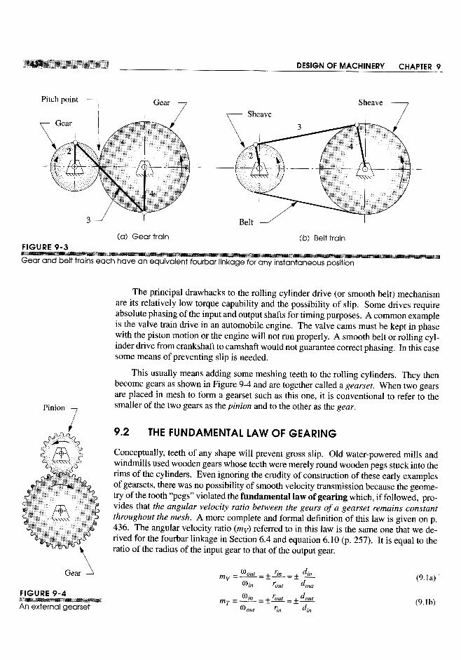


curves at the contact point, and a common normal, perpendicular to the commontangent. Note that the common normal is, in fact, the "strings" of both involutes,which are colinear. Thus the common normal, which is also the axis of transmis-sion, always passes through the pitch point regardless of where in the mesh the twoteeth are contacting.
Figure 9-7 shows a pair of involute tooth forms in two positions, just beginningcontact and about to leave contact. The common normals of both these contactpoints still pass through the same pitch point. It is this property of the involute thatcauses it to obey the fundamental law of gearing. The ratio of the driving gear radius tothe driven gear radius remains constant as the teeth move into and out of mesh.
From this observation of the behavior of the involute we can restate the fund a-mental law of gearing in a more kinematically formal way as: the common normalof the tooth profiles, at all contact points within the mesh, must always pass through afixed point on the line of centers, called the pitch point. The gearset's velocity ratio willthen be a constant defined by the ratio of the respective radii of the gears to the pitchpoint.
The points of beginning and leaving contact define the mesh of the pinion and gear.The distance along the line of action between these points within the mesh is called thelength of action, Z, defined by the intersections of the respective addendum circles withthe line of action, as shown in Figure 9-7.

The distance along the pitch circle within the mesh is the arc of action, and the an-gles subtended by these points and the line of centers are the angle of approach and an-gie of recess. These are shown only on the gear in Figure 9-7 for clarity, but similarangles exist for the pinion. The arc of action on both pinion and gear pitch circles mustbe the same length for zero slip between the theoretical rolling cylinders.
Pressure Angle
The pressure angle in a gearset is similar to that of the cam and follower and is definedas the angle between the axis of transmission or line of action (common normal) and thedirection of velocity at the pitch point as shown in Figures 9-6 and 9-7. Pressure anglesof gearsets are standardized at a few values by the gear manufacturers. These are de-fined at the nominal center distance for the gearset as cut. The standard values are 14.5°,20°, and 25° with 20° being the most commonly used and 14.5° now being consideredobsolete. Any custom pressure angle can be made, but its expense over the availablestock gears with standard pressure angles would be hard to justify. Special cutters wouldhave to be made. Gears to be run together must be cut to the same nominal pressureangle.

Changing Center Distance
When involute teeth (or any teeth) have been cut into a cylinder, with respect to a partic-ular base circle, to create a single gear, we do not yet have a pitch circle. The pitch circleonly comes into being when we mate this gear with another to create a pair of gears, orgearset. There will be some range of center-to-center distances over which we canachieve a mesh between the gears. There will also be an ideal center distance (CD) thatwill give us the nominal pitch diameters for which the gears were designed. However,limitations of manufacturing processes give a low probability that we will be able to ex-actly achieve this ideal center distance in every case. More likely, there will be someerror in the center distance, even if small.
What will happen to the adherence to the fundamental law of gearing if there is er-ror in the location of the gear centers? If the gear tooth form is not an involute, then anerror in center distance will violate the fundamental law, and there will be variation, or"ripple," in the output velocity. The output angular velocity will not be constant for aconstant input velocity. However, with an involute tooth form, center distance errorsdo not affect the velocity ratio. This is the principal advantage of the involute overall other possible tooth forms and the reason why it is nearly universally used for gearteeth. Figure 9-8 shows what happens when the center distance is varied on an invo-lute gearset. Note that the common normal still goes through a pitch point, commonto all contact points within the mesh. But the pressure angle is affected by thechange in center distance.
Figure 9-8 also shows the pressure angles for two different center distances. As thecenter distance increases, so will the pressure angle and vice versa. This is one result ofa change, or error, in center distance when using involute teeth. Note that the fundamen-tal law of gearing still holds in the modified center distance case. The common normalis still tangent to the two base circles and still goes through the pitch point. The pitchpoint has moved, but in proportion to the move of the center distance and the gear radii.The velocity ratio is unchanged despite the shift in center distance. In fact, the velocityratio of involute gears is fixed by the ratio of the base circle diameters, which are un-changing once the gear is cut.
Backlash
Another factor affected by changing center distance is backlash. Increasing the CDwill increase the backlash and vice versa. Backlash is defined as the clearance be-tween mating teeth measured along the circumference of the pitch circle. Manufac-turing tolerances preclude a zero clearance, as all teeth cannot be exactly the samedimensions, and all must mesh. So, there must be some small difference betweenthe tooth thickness and the space width (see Figure 9-9). As long as the gearset isrun with a nonreversing torque, backlash should not be a problem. But, whenevertorque changes sign, the teeth will move from contact on one side to the other. Thebacklash gap will be traversed and the teeth will impact with noticeable noise. Thisis the same phenomenon as crossover shock in the form-closed cam. As well as in-creasing stresses and wear, backlash can cause undesirable positional error in someapplications. If the center distance is set exactly to match the theoretical value forthe gearset, the tooth-to-tooth composite backlash tolerance is in the range of 0.0001

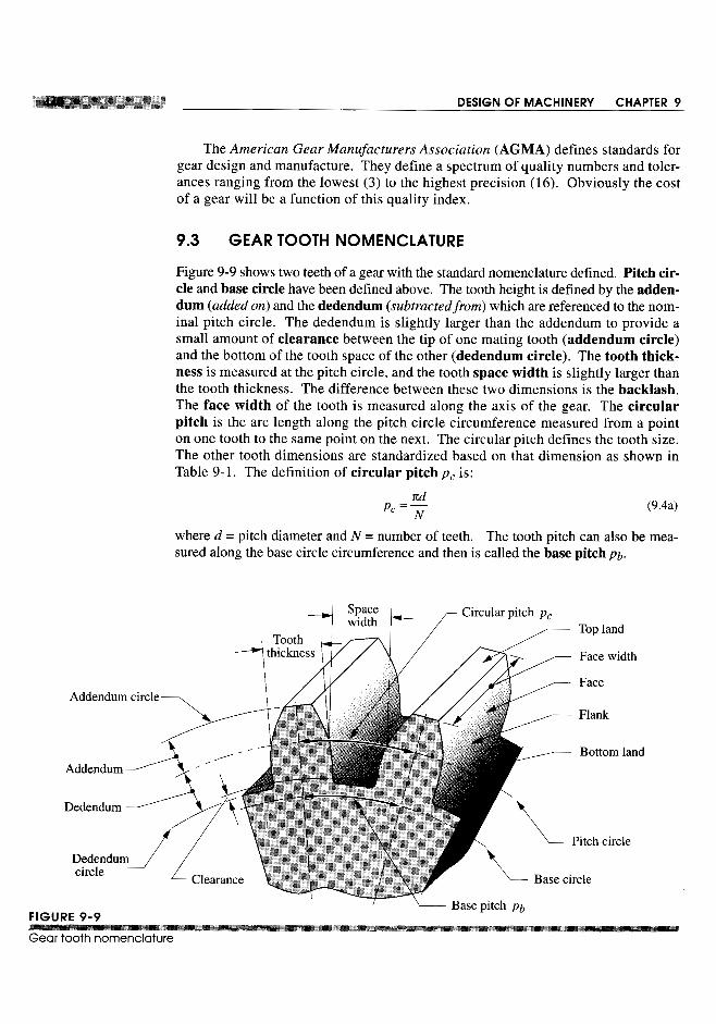


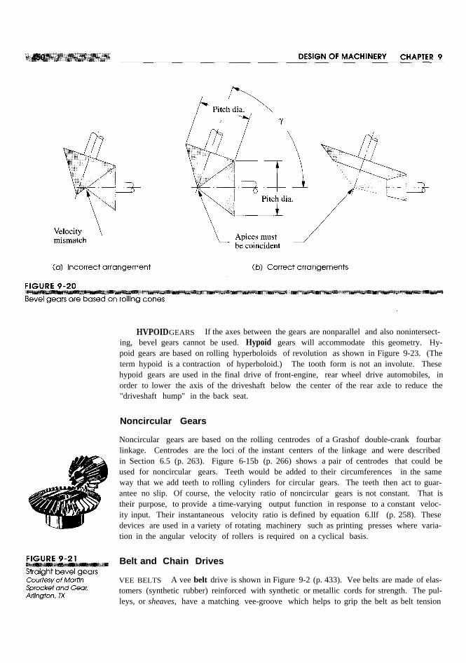
HVPOIDGEARS If the axes between the gears are nonparallel and also nonintersect-ing, bevel gears cannot be used. Hypoid gears will accommodate this geometry. Hy-poid gears are based on rolling hyperboloids of revolution as shown in Figure 9-23. (Theterm hypoid is a contraction of hyperboloid.) The tooth form is not an involute. Thesehypoid gears are used in the final drive of front-engine, rear wheel drive automobiles, inorder to lower the axis of the driveshaft below the center of the rear axle to reduce the"driveshaft hump" in the back seat.
Noncircular Gears
Noncircular gears are based on the rolling centrodes of a Grashof double-crank fourbarlinkage. Centrodes are the loci of the instant centers of the linkage and were describedin Section 6.5 (p. 263). Figure 6-15b (p. 266) shows a pair of centrodes that could beused for noncircular gears. Teeth would be added to their circumferences in the sameway that we add teeth to rolling cylinders for circular gears. The teeth then act to guar-antee no slip. Of course, the velocity ratio of noncircular gears is not constant. That istheir purpose, to provide a time-varying output function in response to a constant veloc-ity input. Their instantaneous velocity ratio is defined by equation 6.llf (p. 258). Thesedevices are used in a variety of rotating machinery such as printing presses where varia-tion in the angular velocity of rollers is required on a cyclical basis.
Belt and Chain Drives
VEE BELTS A vee belt drive is shown in Figure 9-2 (p. 433). Vee belts are made of elas-tomers (synthetic rubber) reinforced with synthetic or metallic cords for strength. The pul-leys, or sheaves, have a matching vee-groove which helps to grip the belt as belt tension


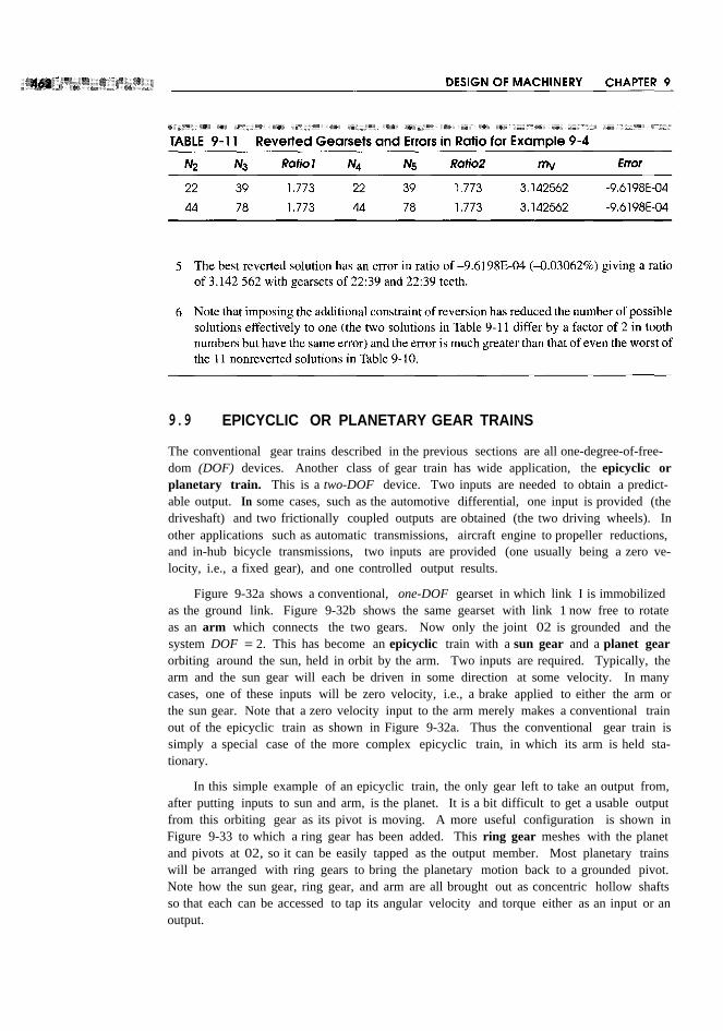
9.9 EPICYCLIC OR PLANETARY GEAR TRAINS
The conventional gear trains described in the previous sections are all one-degree-of-free-dom (DOF) devices. Another class of gear train has wide application, the epicyclic orplanetary train. This is a two-DOF device. Two inputs are needed to obtain a predict-able output. In some cases, such as the automotive differential, one input is provided (thedriveshaft) and two frictionally coupled outputs are obtained (the two driving wheels). Inother applications such as automatic transmissions, aircraft engine to propeller reductions,and in-hub bicycle transmissions, two inputs are provided (one usually being a zero ve-locity, i.e., a fixed gear), and one controlled output results.
Figure 9-32a shows a conventional, one-DOF gearset in which link I is immobilizedas the ground link. Figure 9-32b shows the same gearset with link 1 now free to rotateas an arm which connects the two gears. Now only the joint 02 is grounded and thesystem DOF = 2. This has become an epicyclic train with a sun gear and a planet gearorbiting around the sun, held in orbit by the arm. Two inputs are required. Typically, thearm and the sun gear will each be driven in some direction at some velocity. In manycases, one of these inputs will be zero velocity, i.e., a brake applied to either the arm orthe sun gear. Note that a zero velocity input to the arm merely makes a conventional trainout of the epicyclic train as shown in Figure 9-32a. Thus the conventional gear train issimply a special case of the more complex epicyclic train, in which its arm is held sta-tionary.
In this simple example of an epicyclic train, the only gear left to take an output from,after putting inputs to sun and arm, is the planet. It is a bit difficult to get a usable outputfrom this orbiting gear as its pivot is moving. A more useful configuration is shown inFigure 9-33 to which a ring gear has been added. This ring gear meshes with the planetand pivots at 02, so it can be easily tapped as the output member. Most planetary trainswill be arranged with ring gears to bring the planetary motion back to a grounded pivot.Note how the sun gear, ring gear, and arm are all brought out as concentric hollow shaftsso that each can be accessed to tap its angular velocity and torque either as an input or anoutput.
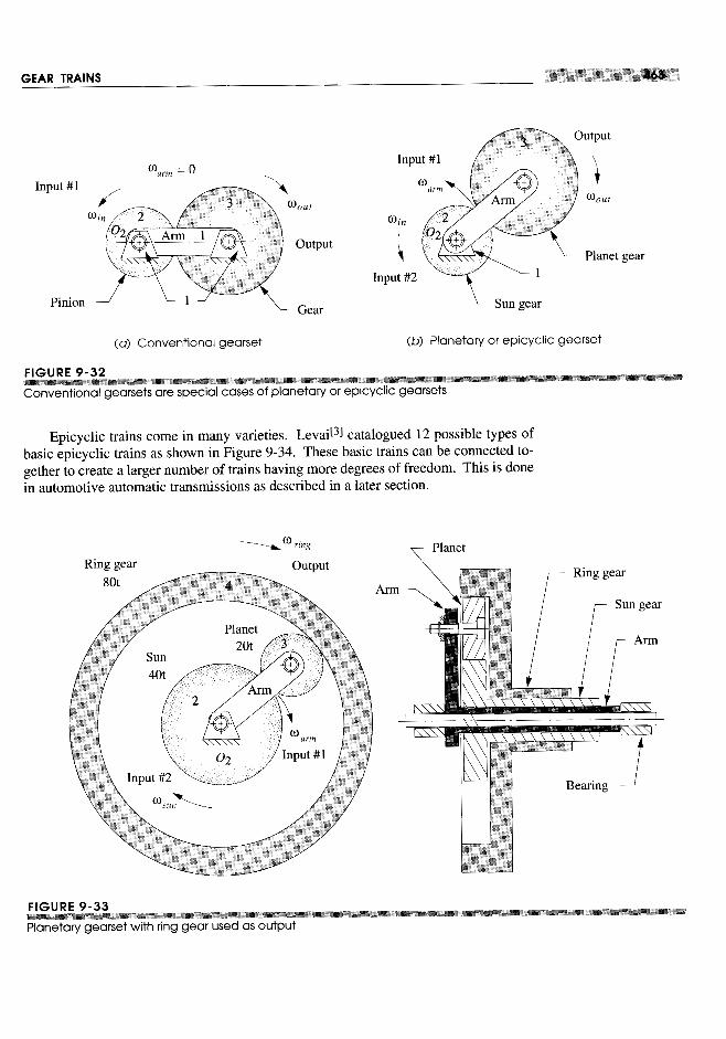


9.11 TRANSMISSIONS
COMPOUND REVERTED GEAR TRAINS are commonly used in manual (nonautomatic)automotive transmissions to provide user-selectable ratios between the engine and thedrive wheels for torque multiplication (mechanical advantage). These gearboxes usuallyhave from three to six forward speeds and one reverse. Most modem transmissions ofthis type use helical gears for quiet operation. These gears are not moved into and out ofengagement when shifting from one speed to another except for reverse. Rather, the de-sired ratio gears are selectively locked to the output shaft by synchromesh mechanisms asin Figure 9-43 which shows a four-speed, manually shifted, synchromesh automotivetransmission.
The input shaft is at top left. The input gear is always in mesh with the left-mostgear on the countershaft at the bottom. This countershaft has several gears integral withit, each of which meshes with a different output gear that is freewheeling on the outputshaft. The output shaft is concentric with the input shaft, making this a reverted train,but the input and output shafts only connect through the gears on the countershaft exceptin "top gear" (fourth speed), for which the input and output shafts are directly coupledtogether with a synchromesh clutch for a I: I ratio.
The synchromesh clutches are beside each gear on the output shaft and are par-tially hidden by the shifting collars which move them left and right in response tothe driver's hand on the shift lever. These clutches act to lock one gear to the outputshaft at a time to provide a power path from input to output of a particular ratio. Thearrows on the figure show the power path for third-speed forward, which is engaged.Reverse gear, on the lower right, engages an idler gear which is physically shiftedinto and out of mesh at standstill.


tionately known as "crashboxes," the name being descriptive of the noise made whenshifting un synchronized gears into and out of mesh while in motion. Henry Ford had abetter idea. His Model T gears were in constant mesh. The two forward speeds and onereverse were achieved by engaging/disengaging a clutch and band brakes in various com-binations via foot pedals. These provided second inputs to the epicyclic train which, likethe Ferguson's paradox, gave bidirectional outputs, all without any "crashing" of gearteeth. This Model T transmission is the precursor to all modern automatic transmissionswhich replace the T's foot pedals with automated hydraulic operation of the clutches andbrakes.
9.12 DIFFERENTIALS
A differential is a device that allows a difference in velocity (and displacement) betweentwo elements. This requires a 2-DOF mechanism such as an epicyclic gear train. Per-haps the most common application of differentials is in the final drive mechanisms ofwheeled land vehicles. When a four-wheeled vehicle turns, the wheels on the outside ofthe turn must travel farther than the inside wheels due to their different turning radii asshown in Figure 9-47. Without a differential mechanism between the inner and outerdriving wheels, the tires must slip on the road surface for the vehicle to turn. If the tireshave good traction, a nondifferentiated drive train will attempt to go in a straight line atall times and will fight the driver in turns. In a four-wheel drive (4WD) vehicle, an ad-ditional differential is needed between the front and rear wheels to allow the wheel ve-locities at each end of the vehicle to vary in proportion to the traction developed at eitherend of the vehicle under slippery conditions. Figure 9-48 shows a 4WD automotivechassis with its three differentials. In this example, the center differential is packagedwith the transmission and front differential but effectively is in the driveshaft betweenthe front and rear wheels as shown in Figure 9-47. Differentials are made with variousgear types. For rear axle applications, a bevel gear epicyclic is commonly used as shownin Figure 9-49a and in Figure P9-3 (p. 482) in the problem section. For center and frontdifferentials, helical or spur gear arrangements are often used as in Figure 9-49b and c.


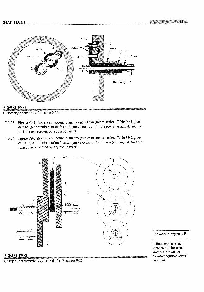


When designing machinery, we must first do a complete kinematic analysis of ourdesign, as described in Part I of this text, in order to obtain information about the accel-erations of the moving parts. We next want to use Newton's second law to calculate thedynamic forces. But to do so we need to know the masses of all the moving parts whichhave these known accelerations. These parts do not exist yet! As with any design prob-lem, we lack sufficient information at this stage of the design to accurately determine thebest sizes and shapes of the parts. We must estimate the masses of the links and otherparts of the design in order to make a first pass at the calculation. We will then have toiterate to better and better solutions as we generate more information. See Section 1.5(p. 7) on the design process to review the use of iteration in design.
A first estimate of your parts' masses can be obtained by assuming some reasonableshapes and sizes for all the parts and choosing appropriate materials. Then calculate thevolume of each part and multiply its volume by the material's mass density (not weightdensity) to obtain a first approximation of its mass. These mass values can then be usedin Newton's equation. The densities of some common engineering materials can befound in Appendix B.
How will we know whether our chosen sizes and shapes of links are even accept-able, let alone optimal? Unfortunately, we will not know until we have carried the com-putations all the way through a complete stress and deflection analysis of the parts. It isoften the case, especially with long, thin elements such as shafts or slender links, that thedeflections of the parts under their dynamic loads will limit the design even at low stresslevels. In some cases the stresses will be excessive.
We will probably discover that the parts fail under the dynamic forces. Then we willhave to go back to our original assumptions about the shapes, sizes, and materials ofthese parts, redesign them, and repeat the force, stress, and deflection analyses. Designis, unavoidably, an iterative process.
The topic of stress and deflection analysis is beyond the scope of this text and willnot be further discussed here. It is mentioned only to put our discussion of dynamic forceanalysis into context. We are analyzing these dynamic forces primarily to provide theinformation needed to do the stress and deflection analyses on our parts! It is also worthnoting that, unlike a static force situation in which a failed design might be fixed by add-ing more mass to the part to strengthen it, to do so in a dynamic force situation can havea deleterious effect. More mass with the same acceleration will generate even higherforces and thus higher stresses! The machine designer often needs to remove mass (inthe right places) from parts in order to reduce the stresses and deflections due to F = ma.Thus the designer needs to have a good understanding of both material properties andstress and deflection analysis to properly shape and size parts for minimum mass whilemaximizing the strength and stiffness needed to withstand the dynamic forces.
10.4 MASS MOMENT AND CENTEROF GRAVITY
When the mass of an object is distributed over some dimensions, it will possess a mo-ment with respect to any axis of choice. Figure 10-1 shows a mass of general shape inan xyz axis system. A differential element of mass is also shown. The mass moment(first moment of mass) of the differential element is equal to the product of its massand its distance from the axis of interest. With respect to the x, y, and z axes these are;
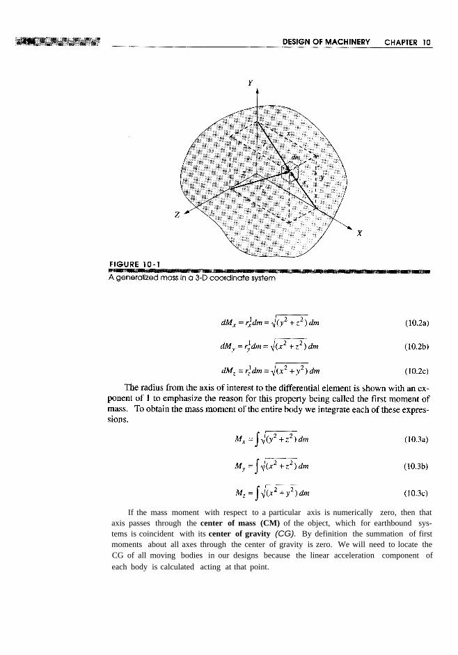
If the mass moment with respect to a particular axis is numerically zero, then thataxis passes through the center of mass (CM) of the object, which for earthbound sys-tems is coincident with its center of gravity (CG). By definition the summation of firstmoments about all axes through the center of gravity is zero. We will need to locate theCG of all moving bodies in our designs because the linear acceleration component ofeach body is calculated acting at that point.


10.8 CENTER OF PERCUSSION
The center of percussion is a point on a body which, when struck with a force, will haveassociated with it another point called the center of rotation at which there will be a zeroreaction force. You have probably experienced the result of "missing the center of per-cussion" when you hit a baseball or softball with the wrong spot on the bat. The "rightplace on the bat" to hit the ball is the center of percussion associated with the point thatyour hands grip the bat (the center of rotation). Hitting the ball at other than the centerof percussion results in a stinging force being delivered to your hands. Hit the right spotand you feel no force (nor pain). The center of percussion is sometimes called the "sweetspot" on a bat, tennis racquet, or golf club. In the case of our mallet example, a center ofpercussion at the head corresponds to a center of rotation near the end of the handle, andthe handle is usually contoured to encourage gripping it there.
The explanation of this phenomenon is quite simple. To make the example two di-mensional and eliminate the effects of friction, consider a hockey stick of mass m lyingon the ice as shown in Figure 1O-3a. Strike it a sharp blow at point P with a force F per-pendicular to the stick axis. The stick will begin to travel across the ice in complex pla-nar motion, both rotating and translating. Its complex motion at any instant can be con-sidered as the superposition of two components: pure translation of its center of gravityG in the direction ofF and pure rotation about that point G. Set up an embedded coordi-


where the radius of gyration k is calculated with respect to the axis ZZ through the CG.
Note that this relationship between the center of percussion and the center of rota-tion involves only geometry and mass properties. The magnitude of the applied force isirrelevant, but its location lp completely determines x. Thus there is not just one centerof percussion on a body. Rather there will be pairs of points. For every point (center ofpercussion) at which a force is applied there will be a corresponding center of rotation atwhich the reaction force felt will be zero. This center of rotation need not fall within thephysical length of the body however. Consider the value of x predicted by equationIO.13b if you strike the body at its CG.
10.9 LUMPED PARAMETER DYNAMIC MODELS
Figure IO-4a shows a simple plate or disk cam driving a spring-loaded, roller follower.This is a force-closed system which depends on the spring force to keep the cam andfollower in contact at all times. Figure 1O-4b shows a lumped parameter model of thissystem in which all the mass which moves with the follower train is lumped together asm, all the springiness in the system is lumped within the spring constant k, and all thedamping or resistance to movement is lumped together as a damper with coefficient c.The sources of mass which contribute to m are fairly obvious. The mass of the followerstem, the roller, its pivot pin, and any other hardware attached to the moving assembly alladd together to create m. Figure 1O-4c shows the free-body diagram of the system actedupon by the cam force Fe, the spring force Fs, and the damping force Fd. There will ofcourse also be the effects of mass times acceleration on the system.
Spring Constant
We have been assuming all links and parts to be rigid bodies in order to do the kinematicanalyses, but to do a more accurate force analysis we need to recognize that these bodies

The total spring constant k of the system is a combination of the spring constants ofthe actual coil spring, plus the spring constants of all other parts which are deflected bythe forces. The roller, its pin, and the follower stem are all springs themselves as theyare made of elastic materials. The spring constant for any part can be obtained from theequation for its deflection under the applied loading. Any deflection equation relatesforce to displacement and can be algebraically rearranged to express a spring constant.An individual part may have more than one k if it is loaded in several modes as, for ex-ample, a camshaft with a spring constant in bending and also one in torsion. We will dis-cuss the procedures for combining these various spring constants in the system togetherinto a combined, effective spring constant k in the next section. For now let us just as-sume that we can so combine them for our analysis and create an overall k for our lumpedparameter model.
Damping
The friction, more generally called damping, is the most difficult parameter of the threeto model. It needs to be a combination of all the damping effects in the system. Thesemay be of many forms. Coulomb friction results from two dry or lubricated surfacesrubbing together. The contact surfaces between cam and follower and between the fol-lower and its sliding joint can experience coulomb friction. It is generally considered tobe independent of velocity magnitude but has a different, larger value when velocity iszero (static friction force Fst or stiction) than when there is relative motion between theparts (dynamic friction Fd). Figure 1O-5a shows a plot of coulomb friction force versusrelative velocity v at the contact surfaces. Note that friction always opposes motion, so

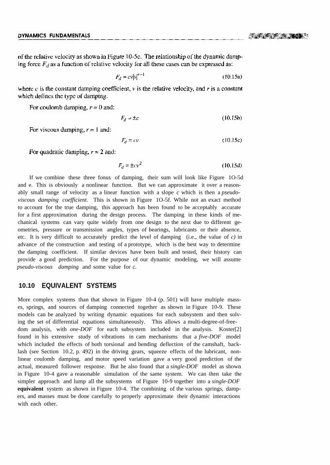
If we combine these three fonus of damping, their sum will look like Figure 1O-5dand e. This is obviously a nonlinear function. But we can approximate it over a reason-ably small range of velocity as a linear function with a slope c which is then a pseudo-viscous damping coefficient. This is shown in Figure 1O-5f. While not an exact methodto account for the true damping, this approach has been found to be acceptably accuratefor a first approximation during the design process. The damping in these kinds of me-chanical systems can vary quite widely from one design to the next due to different ge-ometries, pressure or transmission angles, types of bearings, lubricants or their absence,etc. It is very difficult to accurately predict the level of damping (i.e., the value of c) inadvance of the construction and testing of a prototype, which is the best way to determinethe damping coefficient. If similar devices have been built and tested, their history canprovide a good prediction. For the purpose of our dynamic modeling, we will assumepseudo-viscous damping and some value for c.
10.10 EQUIVALENT SYSTEMS
More complex systems than that shown in Figure 10-4 (p. 501) will have multiple mass-es, springs, and sources of damping connected together as shown in Figure 10-9. Thesemodels can be analyzed by writing dynamic equations for each subsystem and then solv-ing the set of differential equations simultaneously. This allows a multi-degree-of-free-dom analysis, with one-DOF for each subsystem included in the analysis. Koster[2]found in his extensive study of vibrations in cam mechanisms that a five-DOF modelwhich included the effects of both torsional and bending deflection of the camshaft, back-lash (see Section 10.2, p. 492) in the driving gears, squeeze effects of the lubricant, non-linear coulomb damping, and motor speed variation gave a very good prediction of theactual, measured follower response. But he also found that a single-DOF model as shownin Figure 10-4 gave a reasonable simulation of the same system. We can then take thesimpler approach and lump all the subsystems of Figure 10-9 together into a single-DOFequivalent system as shown in Figure 10-4. The combining of the various springs, damp-ers, and masses must be done carefully to properly approximate their dynamic interactionswith each other.
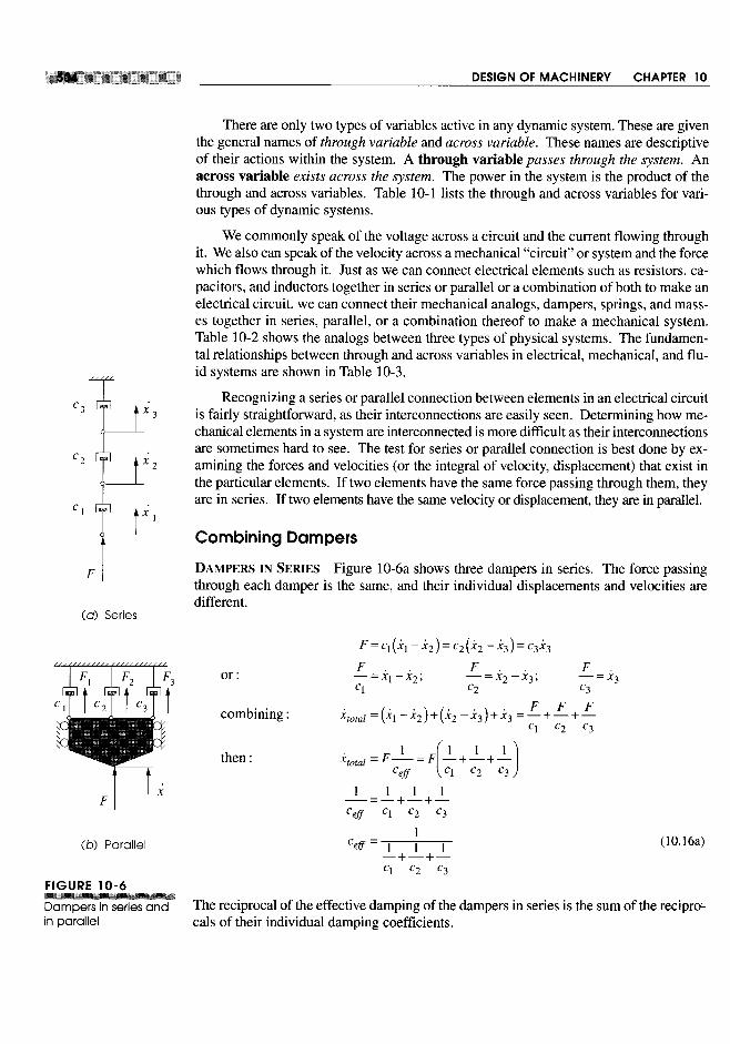


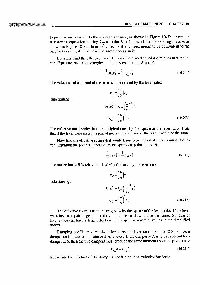


11.0 INTRODUCTION
When kinematic synthesis and analysis have been used to define a geometry and set ofmotions for a particular design task, it is logical and convenient to then use a kinetostat-ic, or inverse dynamics, solution to determine the forces and torques in the system. Wewill take that approach in this chapter and concentrate on solving for the forces andtorques that result from, and are required to drive, our kinematic system in such a way asto provide the designed accelerations. Numerical examples are presented throughout thischapter. These examples are also provided as disk files for input to either program MA-TRIX or FOURBAR. These programs are described in Appendix A. The reader is encour-aged to open the referenced files in these programs and investigate the examples in moredetail. The file names are noted in the discussion of each example.
11.1 NEWTONIAN SOLUTION METHOD
Dynamic force analysis can be done by any of several methods. The one which givesthe most information about forces internal to the mechanism requires only the use ofNewton's law as defined in equations 10.1 (p. 492) and lOA (p. 495). These can be writ-ten as a summation of all forces and torques in the system.
521

These three equations must be written for each moving body in the system whichwill lead to a set of linear simultaneous equations for any system. The set of simulta-neous equations can most conveniently be solved by a matrix method as was shown inChapter 5. These equations do not account for the gravitational force (weight) on a link.If the kinematic accelerations are large compared to gravity, which is often the case, thenthe weight forces can be ignored in the dynamic analysis. If the machine members arevery massive or moving slowly with small kinematic accelerations, or both, the weightof the members may need to be included in the analysis. The weight can be treated as anexternal force acting on the CG of the member at a constant angle.
11.2 SINGLE LINK IN PURE ROTATION
As a simple example of this solution procedure, consider the single link in pure rotationshown in Figure 11-la. In any of these kinetostatic dynamic force analysis problems,the kinematics of the problem must first be fully defined. That is, the angular accelera-tions of all rotating members and the linear accelerations of the CGs of all moving mem-bers must be found for all positions of interest. The mass of each member and the massmoment of inertia 10 with respect to each member's CG must also be known. In addi-tion there may be external forces or torques applied to any member of the system. Theseare all shown in the figure.
While this analysis can be approached in many ways, it is useful for the sake of con-sistency to adopt a particular arrangement of coordinate systems and stick with it. Wepresent such an approach here which, if carefully followed, will tend to minimize thechances of error. The reader may wish to develop his or her own approach once the prin-ciples are understood. The underlying mathematics is invariant, and one can choose co-ordinate systems for convenience. The vectors which are acting on the dynamic systemin any loading situation are the same at a particular time regardless of how we may de-cide to resolve them into components for the sake of computation. The solution resultwill be the same.
We will first set up a nonrotating, local coordinate system on each moving member,located at its CG. (In this simple example we have only one moving member.) All ex-ternally applied forces, whether due to other connected members or to other systemsmust then have their points of application located in this local coordinate system. Fig-ure 11-1b shows a free-body diagram of the moving link 2. The pin joint at 02 on link2 has a force F 12 due to the mating link I, the x and y components of which are F 12x andF 12y' These subscripts are read "force of link I on 2" in the x or y direction. This sub-script notation scheme will be used consistently to indicate which of the "action-reac-tion" pair of forces at each joint is being solved for.


be defined with respect to the link's LNCS. Note that these kinematic and applied forcedata must be available for all positions of the linkage for which a force analysis is de-sired. In the following discussion and examples, only one linkage position will be ad-dressed. The process is identical for each succeeding position and only the calculationsmust be repeated. Obviously, a computer will be a valuable aid in accomplishing thetask.
Link 2 in Figure 11-2b shows forces acting on it at each pin joint, designated F 12and F32. By convention their subscripts denote the force that the adjoining link is exert-ing on the link being analyzed; that is, F 12 is the force of 1 on 2 and F 32 is the force of3on 2. Obviously there is also an equal and opposite force at each of these pins whichwould be designated as F 21 and F 23, respectively. The choice of which of the membersof these pairs of forces to be solved for is arbitrary. As long as proper bookkeeping isdone, their identities will be maintained.
When we move to link 3, we maintain the same convention of showing forces act-ing on the link in its free-body diagram. Thus at instant center !z3 we show F 23 actingon link 3. However, because we showed force F32 acting at the same point on link 2,this introduces an additional unknown to the problem for which we need an additionalequation. The equation is available from Newton's third law:
Thus we are free to substitute the negative reaction force for any action force at anyjoint. This has been done on link 3 in the figure in order to reduce the unknown forces atthat joint to one, namely F 32. The same procedure is followed at each joint with one ofthe action-reaction forces arbitrarily chosen to be solved for and its negative reaction ap-plied to the mating link.
The naming convention used for the position vectors (Rap) which locate the pinjoints with respect to the CG in the link's nonrotating local coordinate system is as fol-lows. The first subscript (a) denotes the adjoining link to which the position vectorpoints. The second subscript ( p) denotes the parent link to which the position vectorbelongs. Thus in the case oflink 2 in Figure 11-2b, vector R 12 locates the attachmentpoint of link 1 to link 2, and R32 the attachment point of link 3 to link 2. Note that insome cases these subscripts will match those of the pin forces shown acting at thosepoints, but where the negative reaction force has been substituted as described above, thesubscript order of the force and its position vector will not agree. This can lead to confu-sion and must be carefully watched for typographical errors when setting up the prob-lem.
Any external forces acting on the links are located in similar fashion with a positionvector to a point on the line of application of the force. This point is given the same let-ter subscript as that of the external force. Link 3 in the figure shows such an externalforce F p acting on it at point P. The position vector Rp locates that point with respect tothe CG. It is important to note that the CG of each link is consistently taken as the pointof reference for all forces acting on that link. Left to its own devices, an unconstrainedbody in complex motion will spin about its own CG; thus we analyze its linear acceler-ation at that point and apply the angular acceleration about the CG as a center.
Equations 11.1 are now written for each moving link. For link 2, with the crossproducts expanded:


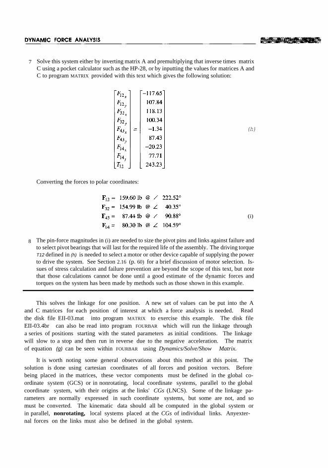
7 Solve this system either by inverting matrix A and premultiplying that inverse times matrixC using a pocket calculator such as the HP-28, or by inputting the values for matrices A andC to program MATRIX provided with this text which gives the following solution:
Converting the forces to polar coordinates:
(h)
(i)
8 The pin-force magnitudes in (i) are needed to size the pivot pins and links against failure andto select pivot bearings that will last for the required life of the assembly. The driving torqueT12 defined in (h) is needed to select a motor or other device capable of supplying the powerto drive the system. See Section 2.16 (p. 60) for a brief discussion of motor selection. Is-sues of stress calculation and failure prevention are beyond the scope of this text, but notethat those calculations cannot be done until a good estimate of the dynamic forces andtorques on the system has been made by methods such as those shown in this example.
This solves the linkage for one position. A new set of values can be put into the Aand C matrices for each position of interest at which a force analysis is needed. Readthe disk file EII-03.mat into program MATRIX to exercise this example. The disk fileEII-03.4br can also be read into program FOURBAR which will run the linkage througha series of positions starting with the stated parameters as initial conditions. The linkagewill slow to a stop and then run in reverse due to the negative acceleration. The matrixof equation (g) can be seen within FOURBAR using Dynamics/Solve/Show Matrix.
It is worth noting some general observations about this method at this point. Thesolution is done using cartesian coordinates of all forces and position vectors. Beforebeing placed in the matrices, these vector components must be defined in the global co-ordinate system (GCS) or in nonrotating, local coordinate systems, parallel to the globalcoordinate system, with their origins at the links' CGs (LNCS). Some of the linkage pa-rameters are normally expressed in such coordinate systems, but some are not, and somust be converted. The kinematic data should all be computed in the global system orin parallel, nonrotating, local systems placed at the CGs of individual links. Anyexter-nal forces on the links must also be defined in the global system.


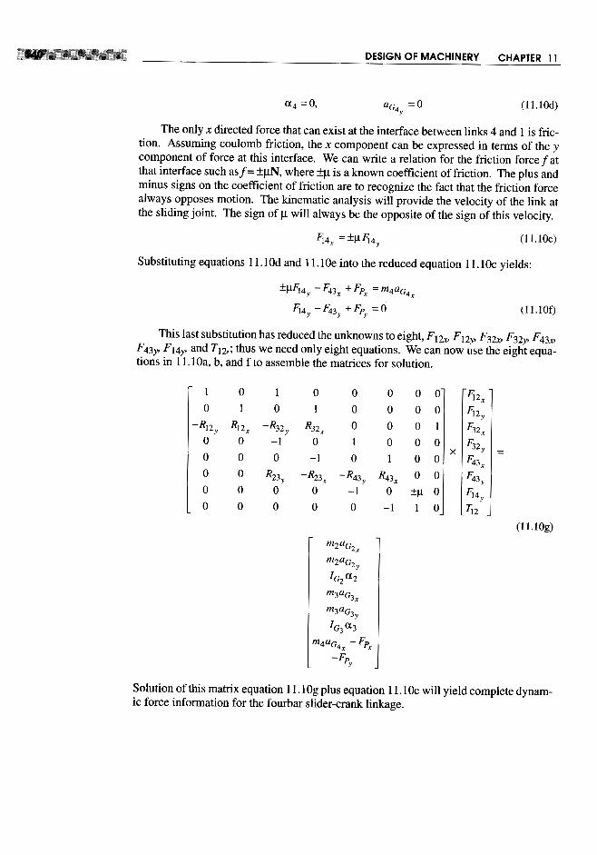


11.11 CONTROLLING INPUT TORQUE-flYWHEElS
The typically large variation in accelerations within a mechanism can cause significantoscillations in the torque required to drive it at a constant or near constant speed. Thepeak torques needed may be so high as to require an overly large motor to deliver them.However, the average torque over the cycle, due mainly to losses and external work done,may often be much smaller than the peak torque. We would like to provide some meansto smooth out these oscillations in torque during the cycle. This will allow us to size themotor to deliver the average torque rather than the peak torque. One convenient and rel-atively inexpensive means to this end is the addition of a flywheel to the system.
TORQUE VARIATION Figure 11-8 shows the variation in the input torque for acrank-rocker fourbar linkage over one full revolution of the drive crank. It is running ata constant angular velocity of 50 rad/sec. The torque varies a great deal within one cy-cle of the mechanism, going from a positive peak of 341.7 Ib-in to a negative peak of-166.41b-in. The average value of this torque over the cycle is only 70.21b-in, beingdue to the external work done plus losses. This linkage has only a 12-lb external forceapplied to link 3 at the CG and a 25 Ib-in external torque applied to link 4. These smallexternal loads cannot account for the large variation in input torque required to maintainconstant crank speed. What then is the explanation? The large variations in torque areevidence of the kinetic energy that is stored in the links as they move. We can think ofthe positive pulses of torque as representing energy delivered by the driver (motor) andstored temporarily in the moving links, and the negative pulses of torque as energy at-tempting to return from the links to the driver. Unfortunately most motors are designedto deliver energy but not to take it back. Thus the "returned energy" has no place to go.
Figure 11-9 shows the speed torque characteristic of a permanent magnet (PM) DCelectric motor. Other types of motors will have differently shaped functions that relatemotor speed to torque as shown in Figure 2-32 and 2-33 (pp. 62-63), but all drivers

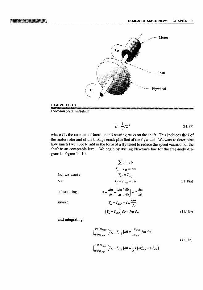


average, the sum of positive area above an average line is equal to the sum of negative areabelow that line.) The integration limits in equation 11.18 are from the shaft angle 8 at whichthe shaft (j)is a minimum to the shaft angle 8 at which (j) is a maximum.
3 The minimum (j)will occur after the maximum positive energy has been delivered from themotor to the load, i.e., at a point (8) where the summation of positive energy (area) in thetorque pulses is at its largest positive value.
4 The maximum (j)will occur after the maximum negative energy has been returned to the load,i.e., at a point (8) where the summation of energy (area) in the torque pulses is at its largestnegative value.
5 To find these locations in 8 corresponding to the maximum and minimum (j)'s and thus findthe amount of energy needed to be stored in the flywheel, we need to numerically integrateeach pulse of this function from crossover to crossover with the average line. The crossoverpoints in Figure 11-11 have been labeled A, B, C, and D. (Program FOURBARdoes this inte-gration for you numerically, using a trapezoidal rule.)
6 The FOURBARprogram prints the table of areas shown in Figure 11-11. The positive andnegative pulses are separately integrated as described above. Reference to the plot of thetorque function will indicate whether a positive or negative pulse is the first encountered ina particular case. The first pulse in this example is a positive one.
7 The remaining task is to accumulate these pulse areas beginning at an arbitrary crossover (inthis case point A) and proceeding pulse by pulse across the cycle. Table 11-1 shows this pro-cess and the result.
8 Note in Table 11-1 that the minimum shaft speed occurs after the largest accumulated posi-tive energy pulse (+200.73 in-lb) has been delivered from the driveshaft to the system. Thisdelivery of energy slows the motor down. The maximum shaft speed occurs after the largestaccumulated negative energy pulse (-60.32 in-lb) has been received back from the systemby the driveshaft. This return of stored energy will speed up the motor. The total energyvariation is the algebraic difference between these two extreme values, which in this exam-ple is -261.05 in-lb. This negative energy coming out of the system needs to be absorbed bythe flywheel and then returned to the system during each cycle to smooth the variations inshaft speed.


the torque curve (see Table 11-1, p. 552) and the average shaft (i) to compute the neededsystem Is. The physical flywheel's mass moment of inertia If is then set equal to the re-quired system Is. But if the moments of inertia of the other rotating elements on the samedriveshaft (such as the motor) are known, the physical flywheel's required If can be re-duced by those amounts.
The most efficient flywheel design in terms of maximizing Iffor minimum materialused is one in which the mass is concentrated in its rim and its hub is supported onspokes, like a carriage wheel. This puts the majority of the mass at the largest radiuspossible and minimizes the weight for a given If Even if a flat, solid circular disk fly-wheel design is chosen, either for simplicity of manufacture or to obtain a flat surfacefor other functions (such as an automobile clutch), the design should be done with an eyeto reducing weight and thus cost. Since in general, I = m,.2, a thin disk of large diame-ter will need fewer pounds of material to obtain a given I than will a thicker disk of small-er diameter. Dense materials such as cast iron and steel are the obvious choices for a fly-wheel. Aluminum is seldom used. Though many metals (lead, gold, silver, platinum) aremore dense than iron and steel, one can seldom get the accounting department's approv-al to use them in a flywheel.
Figure 11-12 shows the change in the input torque T12 for the linkage in Figure 11-8after the addition of a flywheel sized to provide a coefficient of fluctuation of 0.05. Theoscillation in torque about the unchanged average value is now 5%, much less than whatit was without the flywheel. A much smaller horsepower motor can now be used becausethe flywheel is available to absorb the energy returned from the linkage during its cycle.
11.12 A LINKAGE FORCE TRANSMISSION INDEX
The transmission angle was introduced in Chapter 2 and used in subsequent chapters asan index of merit to predict the kinematic behavior of a linkage. A too-small transmis-sion angle predicts problems with motion and force transmission in a fourbar linkage.Unfortunately, the transmission angle has limited application. It is only useful for four-bar linkages and then only when the input and output torques are applied to links that are

pivoted to ground (i.e., the crank and rocker). When external forces are applied to thecoupler link, the transmission angle tells nothing about the linkage's behavior.
Holte and Chase [1] define a joint-force index (IPl) which is useful as an indicatorof any linkage's ability to smoothly transmit energy regardless of where the loads areapplied on the linkage. It is applicable to higher-order linkages as well as to the fourbarlinkage. The IPI at any instantaneous position is defined as the ratio of the maximumstatic force in any joint of the mechanism to the applied external load. If the externalload is a force, then it is:
The F ij are calculated from a static force analysis of the linkage. Dynamic forcescan be much greater than static forces if speeds are high. However, if this static forcetransmission index indicates a problem in the absence of any dynamic forces, then thesituation will obviously be worse at speed. The largest joint force at each position is usedrather than a composite or average value on the assumption that high friction in anyonejoint is sufficient to hamper linkage performance regardless of the forces at other joints.
Equation 11.23a is dimensionless and so can be used to compare linkages of differ-ent design and geometry. Equation 11.23b has dimensions of reciprocal length, so cau-tion must be exercised when comparing designs when the external load is a torque. Thenthe units used in any comparison must be the same, and the compared linkages shouldbe similar in size.
Equations 11.23 apply to anyone instantaneous position of the linkage. As with thetransmission angle, this index must be evaluated for all positions of the linkage over itsexpected range of motion and the largest value of that set found. The peak force maymove from pin to pin as the linkage rotates. If the external loads vary with linkage posi-tion, they can be accounted for in the calculation.
Holte and Chase suggest that the IPI be kept below a value of about 2 for linkageswhose output is a force. Larger values may be tolerable especially if the joints are de-signed with good bearings that are able to handle the higher loads.
There are some linkage positions in which the IPI can become infinite or indetermi-nate as when the linkage reaches an immovable position, defined as the input link or in-put joint being inactive. This is equivalent to a stationary configuration as described inearlier chapters provided that the input joint is inactive in the particular stationary con-figuration. These positions need to be identified and avoided in any event, independentof the determination of any index of merit. In some cases the mechanism may be im-movable but still capable of supporting a load. See reference [1] for more detailed infor-mation on these special cases.

11.13 PRACTICAL CONSIDERATIONS
This chapter has presented some approaches to the computation of dynamic forces inmoving machinery. The newtonian approach gives the most information and is neces-sary in order to obtain the forces at all pin joints so that stress analyses of the memberscan be done. Its application is really quite straightforward, requiring only the creationof correct free-body diagrams for each member and the application of the two simplevector equations which express Newton's second law to each free-body. Once theseequations are expanded for each member in the system and placed in standard matrixform, their solution (with a computer) is a trivial task.
The real work in designing these mechanisms comes in the determination of theshapes and sizes of the members. In addition to the kinematic data, the force computa-tion requires only the masses, CG locations, and mass moments of inertia versus thoseCGs for its completion. These three geometric parameters completely characterize themember for dynamic modelling purposes. Even if the link shapes and materials are com-pletely defined at the outset of the force analysis process (as with the redesign of an ex-isting system), it is a tedious exercise to calculate the dynamic properties of complicatedshapes. Current solids modelling CAD systems make this step easy by computing theseparameters automatically for any part designed within them.
If, however, you are starting from scratch with your design, the blank-paper syn-drome will inevitably rear its ugly head. A first approximation of link shapes and selec-tion of materials must be made in order to create the dynamic parameters needed for a"first pass" force analysis. A stress analysis of those parts, based on the calculated dy-namic forces, will invariably find problems that require changes to the part shapes, thusrequiring recalculation of the dynamic properties and recomputation of the dynamic forc-es and stresses. This process will have to be repeated in circular fashion (iteration-seeChapter 1, p. 8) until an acceptable design is reached. The advantages of using a com-puter to do these repetitive calculations is obvious and cannot be overstressed. An equa-tion solver program such as TKSolver or Mathcad will be a useful aid in this process byreducing the amount of computer programming necessary.
Students with no design experience are often not sure how to approach this processof designing parts for dynamic applications. The following suggestions are offered toget you started. As you gain experience, you will develop your own approach.
It is often useful to create complex shapes from a combination of simple shapes, atleast for first approximation dynamic models. For example, a link could be consideredto be made up of a hollow cylinder at each pivot end, connected by a rectangular prismalong the line of centers. It is easy to calculate the dynamic parameters for each of thesesimple shapes and then combine them. The steps would be as follows (repeated for eachlink):
1 Calculate the volume, mass, CG location, and mass moments of inertia with respectto the local CG of each separate part of your built-up link. In our example link theseparts would be the two hollow cylinders and the rectangular prism.
2 Find the location of the composite CG of the assembly of the parts into the link bythe method shown in Section 11.4 (p. 531) and equation 11.3 (p. 524). See also Fig-ure 11-2 (p. 526).


secZ. There is a vertical force at P of F = 500 N. Find all pin forces and the torqueneeded to drive the crank at this instant.
*t:J:11-12 Figure PII-5b shows a fourbar linkage and its dimensions in meters. The steel crank,coupler, and rocker have uniform cross sections of 50 mm diameter. In the instanta-neous position shown, the crank OzA has 0) = -10 rad/sec and a = 10 rad/sec2. Thereis a horizontal force at P of F = 300 N. Find all pin forces and the torque needed todrive the crank at this instant.
*t:J:11-13 Figure PII-6 shows a water jet loom laybar drive mechanism driven by a pair ofGrashof crank rocker fourbar linkages. The crank rotates at 500 rpm. The laybar iscarried between the coupler-rocker joints of the two linkages at their respectiveinstant centers h,4. The combined weight of the reed and laybar is 29 lb. A 540-lbbeat-up force from the cloth is applied to the reed as shown. The steel links have a 2X I in uniform cross section. Find the forces on the pins for one revolution of thecrank. Find the torque-time function required to drive the system.
tll-14 Figure PII-7 shows a crimping tool. Find the force Fhandneeded to generate a 2000-Ib Fcrimp' Find the pin forces. What is this linkage's joint force transmission index(IFI) in this position?
t§ 11-15 Figure P 11-8 shows a walking beam conveyor mechanism that operates at slow speed(25 rpm). The boxes being pushed each weigh 50 lb. Determine the pin forces in thelinkage and the torque required to drive the mechanism through one revolution.Neglect the masses of the links.
t§ 11-16 Figure PII-9 shows a surface grinder table drive that operates at 120 rpm. The crankradius is 22 mm, the coupler is 157 mm, and its offset is 40 mm. The mass of tableand workpiece combined is 50 kg. Find the pin forces, slider side loads, and drivingtorque over one revolution.
t§1l-17 Figure Pll-1O shows a power hacksaw that operates at 50 rpm. The crank is 75 mm,the coupler is 170 mm, and its offset is 45 mm. Find the pin forces, slider side loads,and driving torque over one revolution for a cutting force of 250 N in the forwarddirection and 50 N during the return stroke.

t§11-18 Figure Pll-ll shows a paper roll off-loading station. The paper rolls have a 0.9-mOD, 0.22-m ID, are 3.23 m long, and have a density of 984 kg/m3. The forks thatsupport the roll are 1.2 m long. The motion is slow so inertial loading can beneglected. Find the force required of the air cylinder to rotate the roll through 90°.
t 11-19 Derive an expression for the relationship between flywheel mass and the dimension-less parameter radius/thickness (r/t) for a solid disk flywheel of moment of inertia f.Plot this function for an arbitrary value of f and determine the optimum r/t ratio tominimize flywheel weight for that f.


The following problem statement applies to all the projects listed.These larger-scale project statements deliberately lack detail and structure and areloosely defined. Thus, they are similar to the kind of "identification of need " or problemstatement commonly encountered in engineering practice. It is left to the student to struc-ture the problem through background research and to create a clear goal statement andset of performance specifications before attempting to design a solution. This designprocess is spelled out in Chapter 1 and should befollowed in all of these examples. Allresults should be documented in a professional engineering report. See the Bibliogra-phy in Chapter 1 for references on report writing.
Some of these project problems are based on the kinematic design projects in Chap-ter 3. Those kinematic devices can now be designed more realistically with considerationof the dynamic forces that they generate. The strategy in most of the following projectproblems is to keep the dynamic pin forces and thus the shaking forces to a minimum andalso keep the input torque-time curve as smooth as possible to minimize power require-ments. All these problems can be solved with a pin-jointed fourbar linkage. This factwill allow you to use program FOURBAR to do the kinematic and dynamic computationson a large number and variety of designs in a short time. There are infinities of viablesolutions to these problems. Iterate to find the best one! All links must be designed indetail as to their geometry (mass, moment of inertia, etc.). An equation solver such asMathcad or TKSolver will be useful here. Determine all pin forces, shaking force, shak-ing torque, and input horsepower required for your designs.
Pll-l Project P3-1 stated that:
The tennis coach needs a better tennis ball server for practice. This device must fire asequence of standard tennis balls from one side of a standard tennis court over the netsuch that they land and bounce within each of the three court areas defined by thecourt's white lines. The order and frequency of a ball's landing in anyone of thethree court areas must be random. The device should operate automatically andunattended except for the refill of balls. It should be capable of firing 50 ballsbetween reloads. The timing of ball releases should vary. For simplicity, a motor-driven pin-jointed linkage design is preferred.
This project asks you to design such a device to be mounted upon a tripod stand of5-foot height. Design it, and the stand, for stability against tipover due to the shakingforces and shaking torques which should also be minimized in the design of yourlinkage. Minimize the input torque required.
PII-2 Project P3-9 stated that:
The "Save the Skeet" foundation has requested a more humane skeet launcher bedesigned. While they have not yet succeeded in passing legislation to prevent thewholesale slaughter of these little devils, they are concerned about the inhumaneaspects of the large accelerations imparted to the skeet as it is launched into the skyfor the sportsperson to shoot it down. The need is for a skeet launcher that willsmoothly accelerate the clay pigeon onto its desired trajectory.

Design a skeet launcher to be mounted upon a child's "little red wagon." Controlyour design parameters so as to minimize the shaking forces and torques so that thewagon will remain as nearly stationary as possible during the launch of the claypigeon.
Pl1-3 Project P3-10 stated that:
The coin-operated "kid bouncer" machines found outside supermarkets typicallyprovide a very unimaginative rocking motion to the occupant. There is a need for asuperior "bouncer" which will give more interesting motions while remaining safe forsmall children.
Design this device for mounting in the bed of a pickup truck. Keep the shakingforces to a minimum and the input torque-time curve as smooth as possible.
Pl1-4 Project P3-15 stated that:
NASA wants a zero-G machine for astronaut training. It must carry one person andprovide a negative l-g acceleration for as long as possible.Design this device and its mounting hardware to the ground plane minimizing thedynamic forces and driving torque.
Pl1-5 Project P3-16 stated that:
The Amusement Machine Co. Inc. wants a portable "WHIP" ride which will give twoor four passengers a thrilling but safe ride and which can be trailed behind a pickuptruck from one location to another.
Design this device and its mounting hardware to the truck bed minimizing thedynamic forces and driving torque.
P 11-6 Project P3-17 stated that:
The Air Force has requested a pilot training simulator which will give potential pilotsexposure to G forces similar to those they will experience in dogfight maneuvers.Design this device and its mounting hardware to the ground plane minimizing thedynamic forces and driving torque.
Pl1-7 Project P3-18 stated that:
Cheers needs a better "mechanical bull" simulator for their "yuppie" bar in Boston. Itmust give a thrilling "bucking bronco" ride but be safe.Design this device and its mounting hardware to the ground plane minimizing thedynamic forces and driving torque.
Pll-8 Gargantuan Motors Inc. is designing a new light military transport vehicle. Theircurrent windshield wiper linkage mechanism develops such high shaking forces whenrun at its highest speed that the engines are falling out! Design a superior windshieldwiper mechanism to sweep the 20-lb armored wiper blade through a 90° arc whileminimizing both input torque and shaking forces. The wind load on the blade,perpendicular to the windshield, is 50 lb. The coefficient of friction of the wiperblade on glass is 0.9.

PII-9 The Anny's latest helicopter gunship is to be fitted with the Gatling gun, which fires
50-mm-diameter, 2-cm-long spent uranium slugs at a rate of 10 rounds per second.
The reaction (recoil) force may upset the chopper's stability. A mechanism is needed
which can be mounted to the frame of the helicopter and which will provide a
synchronous shaking force, 1800 out of phase with the recoil force pulses, to
counteract the recoil of the gun. Design such a linkage and minimize its torque and
power drawn from the aircraft's engine. Total weight of your device should also beminimized.
Pll-1O Steel pilings are universally used as foundations for large buildings. These are often
driven into the ground by hammer blows from a "pile driver." In certain soils (sandy,
muddy) the piles can be "shaken" into the ground by attaching a "vibratory driver"
which imparts a vertical, dynamic shaking force at or near the natural frequency of
the pile-earth system. The pile can literally be made to "fall into the ground" under
optimal conditions. Design a fourbar linkage-based pile shaker mechanism which,
when its ground link is finnly attached to the top of a piling (supported from a crane
hook), will impart a dynamic shaking force that is predominantly directed along the
piling's long, vertical axis. Operating speed should be in the vicinity of the naturalfrequency of the pile-earth system.
Pll-ll Paint can shaker mechanisms are common in paint and hardware stores. While they
do a good job of mixing the paint, they are also noisy and transmit their vibrations to
the shelves and counters. A better design of the paint can shaker is possible using a
balanced fourbar linkage. Design such a portable device to sit on the floor (not
bolted down) and minimize the shaking forces and vibrations while still effectivelymixing the paint.
PII-12 Convertible automobiles are once again popular. While offering the pleasure of
open-air motoring, they offer little protection to the occupants in a rollover accident.
Pennanent roll bars are ugly and detract from the open feeling of a true convertible.
An automatically deployable roll bar mechanism is needed that will be out of sight
until needed. In the event that sensors in the vehicle detect an imminent rollover, the
mechanism should deploy within 250 ms. Design a collapsible/deployable roll barmechanism to retrofit to the convertible of your choice.

12.0 INTRODUCTIONAny link or member that is in pure rotation can, theoretically, be perfectly balanced toeliminate all shaking forces and shaking moments. It is accepted design practice to bal-ance all rotating members in a machine unless shaking forces are desired (as in a vibrat-ing shaker mechanism, for example). A rotating member can be balanced either statical-ly or dynamically. Static balance is a subset of dynamic balance. To achieve completebalance requires that dynamic balancing be done. In some cases, static balancing can bean acceptable substitute for dynamic balancing and is generally easier to do.
Rotating parts can, and generally should, be designed to be inherently balanced bytheir geometry. However, the vagaries of production tolerances guarantee that there willstill be some small unbalance in each part. Thus a balancing procedure will have to beapplied to each part after manufacture. The amount and location of any imbalance canbe measured quite accurately and compensated for by adding or removing material in the
correct locations.In this chapter we will investigate the mathematics of determining and designing a
state of static and dynamic balance in rotating elements and also in mechanisms havingcomplex motion, such as the fourbar linkage. The methods and equipment used to mea-

sure and correct imbalance in manufactured assemblies will also be discussed. It is quiteconvenient to use the method of d' Alembert (see Section 10.12, p. 513) when discussingrotating imbalance, applying inertia forces to the rotating elements, so we will do that.
12.1 STATIC BALANCE
Despite its name, static balance does apply to things in motion. The unbalanced forcesof concern are due to the accelerations of masses in the system. The requirement forstatic balance is simply that the sum of all forces on the moving system (includingd'Alembert inertial forces) must be zero.
This, of course, is simply a restatement of Newton's law as discussed in Section 10.1 (p. 491).
Another name for static balance is single-plane balance, which means that themasses which are generating the inertia forces are in, or nearly in, the same plane. It isessentially a two-dimensional problem. Some examples of common devices which meetthis criterion, and thus can successfully be statically balanced, are: a single gear or pul-ley on a shaft, a bicycle or motorcycle tire and wheel, a thin flywheel, an airplane pro-peller, an individual turbine blade-wheel (but not the entire turbine). The common de-nominator among these devices is that they are all short in the axial direction comparedto the radial direction, and thus can be considered to exist in a single plane. An automo-bile tire and wheel is only marginally suited to static balancing as it is reasonably thickin the axial direction compared to its diameter. Despite this fact, auto tires are sometimesstatically balanced. More often they are dynamically balanced and will be discussedunder that topic.
Figure l2-la shows a link in the shape of a vee which is part of a linkage. We wantto statically balance it. We can model this link dynamically as two point masses ml andm2 concentrated at the local CGs of each "leg" of the link as shown in Figure l2-lb.These point masses each have a mass equal to that of the "leg" they replace and are sup-ported on massless rods at the position (R1 or R2) ofthat leg's CG. We can solve for therequired amount and location of a third "balance mass" mb to be added to the system atsome location Rb in order to satisfy equation 12.1.
Assume that the system is rotating at some constant angular velocity 00. The accel-erations of the masses will then be strictly centripetal (toward the center) , and the iner-tia forces will be centrifugal (away from the center) as shown in Figure 12-1. Since thesystem is rotating, the figure shows a "freeze-frame" image of it. The position at whichwe "stop the action" for the purpose of drawing the picture and doing the calculations isboth arbitrary and irrelevant to the computation. We will set up a coordinate system withits origin at the center of rotation and resolve the inertial forces into components in thatsystem. Writing vector equation 12.1 for this system we get:
Note that the only forces acting on this system are the inertia forces. For balancing,it does not matter what external forces may be acting on the system. External forcescannot be balanced by making any changes to the system's internal geometry. Note thatthe ro2 terms cancel. For balancing, it also does not matter how fast the system is rotat-


These moments act in planes that include the axis of rotation of the assembly suchas planes XZ and YZ in Figure 12-2. The moment's vector direction, or axis, is perpen-dicular to the assembly's axis of rotation.
Any rotating object or assembly which is relatively long in the axial direction com-pared to the radial direction requires dynamic balancing for complete balance. It is pos-sible for an object to be statically balanced but not be dynamically balanced. Considerthe assembly in Figure 12-2. TWo equal masses are at identical radii, 1800 apart rota-tionally, but separated along the shaft length. A summation of -ma forces due to theirrotation will be always zero. However, in the side view, their inertia forces form a cou-ple which rotates with the masses about the shaft. This rocking couple causes a momenton the ground plane, alternately lifting and dropping the left and right ends of the shaft.
Some examples of devices which require dynamic balancing are: rollers, crank-shafts, camshafts, axles, clusters of multiple gears, motor rotors, turbines, propellershafts. The common denominator among these devices is that their mass may be uneven-ly distributed both rotationally around their axis and also longitudinally along their axis.
To correct dynamic imbalance requires either adding or removing the right amountof mass at the proper angular locations in two correction planes separated by some dis-tance along the shaft. This will create the necessary counter forces to statically balancethe system and also provide a counter couple to cancel the unbalanced moment. Whenan automobile tire and wheel is dynamically balanced, the two correction planes are theinner and outer edges of the wheel rim. Correction weights are added at the proper loca-tions in each of these correction planes based on a measurement of the dynamic forcesgenerated by the unbalanced, spinning wheel.


So, when the design is still on the drawing board, these simple analysis techniquescan be used to determine the necessary sizes and locations of balance masses for anyassembly in pure rotation for which the mass distribution is defined. This two-planebalance method can be used to dynamically balance any system in pure rotation, and allsuch systems should be balanced unless the purpose of the device is to create shakingforces or moments.
12.3 BALANCING LINKAGES
Many methods have been devised to balance linkages. Some achieve a complete bal-ance of one dynamic factor, such as shaking force, at the expense of other factors suchas shaking moment or driving torque. Others seek an optimum arrangement that collec-tively minimizes (but does not zero) shaking forces, moments, and torques for a bestcompromise. Lowen and Berkof, [1] and Lowen, Tepper, and Berkof [2] give compre-hensive reviews of the literature on this subject up to 1983. Additional work has beendone on the problem since that time, some of which is noted in the references at the endof this chapter.
Complete balance of any mechanism can be obtained by creating a second "mirrorimage" mechanism connected to it so as to cancel all dynamic forces and moments.Certain configurations of multicylinder internal combustion engines do this. The pistonsand cranks of some cylinders cancel the inertial effects of others. We will explore theseengine mechanisms in Chapter 14. However, this approach is expensive and is only jus-tified if the added mechanism serves some second purpose such as increasing power, asin the case of additional cylinders in an engine. Adding a "dummy" mechanism whoseonly purpose is to cancel dynamic effects is seldom economically justifiable.
Most practical linkage balancing schemes seek to minimize or eliminate one or moreof the dynamic effects (forces, moments, torques) by redistributing the mass of the ex-isting links. This typically involves adding counterweights and/or changing the shapesof links to relocate their CGs. More elaborate schemes add geared counterweights tosome links in addition to redistributing their mass. As with any design endeavor, thereare trade-offs. For example, elimination of shaking forces usually increases the shakingmoment and driving torque. We can only present a few approaches to this problem inthe space available. The reader is directed to the literature for information on other methods.


We now have two equations involving three links. The parameters for anyone linkcan be assumed and the other two solved for. A linkage is typically first designed to sat-isfy the required motion and packaging constraints before this force balancing procedureis attempted. In that event, the link geometry and masses are already defined, at least ina preliminary way. A useful strategy is to leave the link 3 mass and CG location as orig-inally designed and calculate the necessary masses and CG locations of links 2 and 4 tosatisfy these conditions for balanced forces. Links 2 and 4 are in pure rotation, so it isstraightforward to add counterweights to them in order to move their CGs to the neces-sary locations. With this approach, the right sides of equations 12.8b are reducible tonumbers for a designed linkage. We want to solve for the mass radius products m2b2 andm4b4 and also for the angular locations of the CGs within the links. Note that the angles<1>2 and <1>4 in equation 12.8 are measured with respect to the lines of centers of their re-spective links.
Equations 12.8b are vector equations. Substitute the Euler identity (equation 4.4a,p. 155) to separate into real and imaginary components, and solve for the x and y compo-nents of the mass-radius products.

These components of the mR product needed to force balance the linkage representthe entire amount needed. If links 2 and 4 are already designed with some individualunbalance (the CG not at pivot), then the existing mR product of the unbalanced link mustbe subtracted from that found in equations 12.8c and 12.8d in order to determine the sizeand location of additional counterweights to be added to those links. As we did with thebalance of rotating links, any combination of mass and radius that gives the desired prod-uct is acceptable. Use equations 12.2d and 12.2e to convert the cartesian mR products inequations 12.8c and 12.8d to polar coordinates in order to find the magnitude and angleof the counterweight's mR vector. Note that the angle of the mR vector for each link willbe referenced to that link's line of centers. Design the shape of the physical counter-weights to be put on the links as discussed in Section 12.1 (p. 571).
12.4 EFFECTOF BALANCING ON SHAKING AND PIN FORCES
Figure 12-5 shows a fourbar linkage* to which balance masses have been added in ac-cord with equations 12.8. Note the counterweights placed on links 2 and 4 at the calcu-lated locations for complete force balance. Figure 12-6a shows a polar plot of the shak-ing forces of this linkage without the balance masses. The maximum is 462 Ib at 15°.Figure 12-6b shows the shaking forces after the balance masses are added. The shakingforces are reduced to essentially zero. The small residual forces seen in Figure 12-6bare due to computational round-off errors-the method gives theoretically exact results.

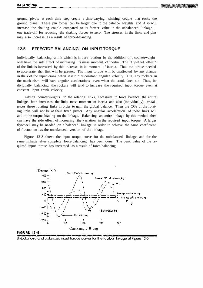
ground pivots at each time step create a time-varying shaking couple that rocks theground plane. These pin forces can be larger due to the balance weights and if so willincrease the shaking couple compared to its former value in the unbalanced linkage-one trade-off for reducing the shaking forces to zero. The stresses in the links and pinsmay also increase as a result of force-balancing.
12.5 EFFECTOF BALANCING ON INPUT TORQUE
Individually balancing a link which is in pure rotation by the addition of a counterweightwill have the side effect of increasing its mass moment of inertia. The "flywheel effect"of the link is increased by this increase in its moment of inertia. Thus the torque neededto accelerate that link will be greater. The input torque will be unaffected by any changein the I of the input crank when it is run at constant angular velocity. But, any rockers inthe mechanism will have angular accelerations even when the crank does not. Thus, in-dividually balancing the rockers will tend to increase the required input torque even atconstant input crank velocity.
Adding counterweights to the rotating links, necessary to force balance the entirelinkage, both increases the links mass moment of inertia and also (individually) unbal-ances those rotating links in order to gain the global balance. Then the CGs of the rotat-ing links will not be at their fixed pivots. Any angular acceleration of these links willadd to the torque loading on the linkage. Balancing an entire linkage by this method thencan have the side effect of increasing the variation in the required input torque. A largerflywheel may be needed on a balanced linkage in order to achieve the same coefficientof fluctuation as the unbalanced version of the linkage.
Figure 12-8 shows the input torque curve for the unbalanced linkage and for thesame linkage after complete force-balancing has been done. The peak value of the re-quired input torque has increased as a result of force-balancing.

Note, however, that the degree of increase in the input torque due to force-balanc-ing is dependent upon the choice of radii at which the balance masses are placed. Theextra mass moment of inertia that the balance mass adds to a link is proportional to thesquare of the radius to the CG of the balance mass. The force balance algorithm onlycomputes the required mass-radius product. Placing the balance mass at as small a radi-us as possible will minimize the increase in input torque. Weiss and Fenton [5J haveshown that a circular counterweight placed tangent to the link's pivot center (Figure 12-9)is a good compromise between added weight and increased moment of inertia. To re-duce the torque penalty further, one could also choose to do less than a complete forcebalance and accept some shaking force in trade.
where TZI is the negative of the driving torque T12' Rl is the position vector from Oz to04 (i.e., link 1), and F41 is the force of the rocker on the ground plane. In a general link-age, the magnitude of the shaking moment can be reduced but cannot be eliminated bymeans of mass redistribution within its links. Complete balancing of the shaking mo-ment requires the addition of supplementary links and then only works for certain spe-cial configurations of a fourbar linkage.[7]
Many techniques have been developed that use optimization methods to find a link-age mass configuration that will minimize the shaking moment alone or in combinationwith minimizing shaking force and/or input torque. Hockey [8J, [9J shows that the fluc-tuation in kinetic energy and input torque of a mechanism may be reduced by proper dis-tribution of mass within its links and that this approach is more weight efficient than add-ing a flywheel to the input shaft. Berkof [10] also describes a method to minimize theinput torque by internal mass rearrangement. Lee and Cheng [11] and Qi and Pen-nestri [1zJ show methods to optimally balance the combined shaking force, shaking mo-ment, and input torque in high-speed linkages by mass redistribution and addition ofcounterweights. Porter [13] suggests using a genetic algorithm to optimize the same setof parameters. Bagci [14J describes several approaches to balancing shaking forces andshaking moments in the fourbar slider-crank linkage. Most of these methods require sig-nificant computing resources, and space does not permit a complete discussion of themall here. The reader is directed to the references for more information.
Berkofs method for complete moment balancing of the fourbar linkage [7]is simpleand useful even though it is limited to "inline" linkages, i.e., those whose link CGs lie ontheir respective link centerlines as shown in Figure 12-9. This is not an overly restric-tive constraint since many practical linkages are made with straight links. Even if a linkmust have a shape that deviates from its line of centers, its CG can still be placed on thatline by adding mass to the link in the proper location, increased weight being the trade-off.
For complete moment balancing, in addition to being an inline linkage, the couplermust be reconfigured to become a physical pendulum such that it is dynamically equiv-alent to a lumped mass model as shown in Figure 12-10. The coupler is shown in Figure


terweight can balance any planar moment that is proportional to an angular accelerationand does not introduce any net inertia, forces to upset the force balance of the linkage.Trade-offs include increased input torque and larger pin forces resulting from the torquerequired to accelerate the additional rotational inertia. There can also be large loads on thegear teeth and impact when torque reversals take up the gearsets' backlash, causing noise.
The shaking moment of an inline fourbar linkage is derived in reference [6] as
Equations l2.l7a and l2.l7b are the force-balance criteria of equation 12.8 writtenfor the inline linkage case. Equation l2.l7c defines the coupler as a physical pendulum.Equations l2.l7d and l2.l7e define the mass moments of inertia required for the twoinertia counterweights. Note that if the linkage is run at constant angular velocity, a2will be zero in equation 12.14 and the inertia counterweight on link 2 can be omitted.

12.7 MEASURING AND CORRECTING IMBALANCE
While we can do a great deal to ensure balance when designing a machine, variationsand tolerances in manufacturing will preclude even a well-balanced design from beingin perfect balance when built. Thus there is need for a means to measure and correct theimbalance in rotating systems. Perhaps the best example assembly to discuss is that ofthe automobile tire and wheel, with which most readers will be familiar. Certainly thedesign of this device promotes balance, as it is essentially cylindrical and symmetrical.If manufactured to be perfectly uniform in geometry and homogeneous in material, itshould be in perfect balance as is. But typically it is not. The wheel (or rim) is morelikely to be close to balanced, as manufactured, than is the tire. The wheel is made of ahomogeneous metal and has fairly uniform geometry and cross section. The tire, how-ever, is a composite of synthetic rubber elastomer and fabric cord or metal wire. Thewhole is compressed in a mold and steam-cured at high temperature. The resulting ma-terial varies in density and distribution, and its geometry is often distorted in the processof removal from the mold and cooling.
STATIC BALANCING After the tire is assembled to the wheel, the assembly mustbe balanced to reduce vibration at high speeds. The simplest approach is to statically bal-ance it, though it is not really an ideal candidate for this approach as it is thick axiallycompared to its diameter. To do so it is typically suspended in a horizontal plane on acone through its center hole. A bubble level is attached to the wheel, and weights areplaced at positions around the rim of the wheel until it sits level. These weights are thenattached to the rim at those points. This is a single-plane balance and thus can only can-cel the unbalanced forces. It has no effect on any unbalanced moments due to unevendistribution of mass along the axis of rotation. It also is not very accurate.
DYNAMIC BALANCING The better approach is to dynamically balance it. Thisrequires a dynamic balancing machine be used. Figure 12-12 shows a schematic of sucha device used for balancing wheels and tires or any other rotating assembly. The assem-bly to be balanced is mounted temporarily on an axle, called a mandrel, which is sup-ported in bearings within the balancer. These two bearings are each mounted on a sus-pension which contains a transducer that measures dynamic force. A common type offorce transducer contains a piezoelectric crystal which delivers a voltage proportional tothe force applied. This voltage is amplified electronically and delivered to circuitry orsoftware which can compute its peak magnitude and the phase angle of that peak withrespect to some time reference signal. The reference signal is supplied by a shaft encod-er on the mandrel which provides a short duration electrical pulse once per revolution inexactly the same angular location. This encoder pulse triggers the computer to beginprocessing the force signal. The encoder may also provide some large number of addi-tional pulses equispaced around the shaft circumference (often 1024). These are used totrigger the recording of each data sample from the transducers in exactly the same loca-tion around the shaft and to provide a measure of shaft velocity via an electronic counter.
The assembly to be balanced is then "spun up" to some angular velocity, usuallywith a friction drive contacting its circumference. The drive torque is then removed andthe drive motor stopped, allowing the assembly to "freewheel." (This is to avoid mea-suring any forces due to imbalances in the drive system.) The measuring sequence isbegun, and the dynamic forces at each bearing are measured simultaneously and theirwaveforms stored. Many cycles can be measured and averaged to improve the quality

of the measurement. Because forces are being measured at two locations displaced alongthe axis, both summation of moment and summation of force data are computed.
The force signals are sent to a built-in computer for processing and computation ofthe needed balance masses and locations. The data needed from the measurements arethe magnitudes of the peak forces and the angular locations of those peaks with respectto the shaft encoder's reference angle (which corresponds to a known point on thewheel). The axial locations of the wheel rim's inside and outside edges (the correctionplanes) with respect to the balance machine's transducer locations are provided to themachine's computer by operator measurement. From these data the net unbalanced forceand net unbalanced moment can be calculated since the distance between the measuredbearing forces is known. The mass-radius products needed in the correction planes oneach side of the wheel can then be calculated from equations 12.3 (p. 574) in terms ofthe mR product of the balance weights. The correction radius is that of the wheel rim.The balance masses and angular locations are calculated for each correction plane to putthe system in dynamic balance. Weights having the needed mass are clipped onto theinside and outside wheel rims (which are the correction planes in this case), at the properangular locations. The result is a fairly accurately dynamically balanced tire and wheel.


13.0 INTRODUCTION
The previous chapters have introduced analysis techniques for the determination of dy-namic forces, moments, and torques in machinery. Shaking forces, moments, and theirbalancing have also been discussed. We will now attempt to integrate all these dynamicconsiderations into the design of a common device, the slider-crank linkage as used inthe internal combustion engine. This deceptively simple mechanism will be found to beactually quite complex in terms of the dynamic considerations necessary to its design forhigh-speed operation. Thus it will serve as an excellent example of the application ofthe dynamics concepts just presented. We will not address the thermodynamic aspectsof the internal combustion engine beyond defining the combustion forces which are nec-essary to drive the device. Many other texts, such as those listed in the bibliography atthe end of this chapter, deal with the very complex thermodynamic and fluid dynamicaspects of this ubiquitous device. We will concentrate only on its kinematics and me-chanical dynamics aspects. It is not our intention to make an "engine designer" of thestudent so much as to apply dynamic principles to a realistic design problem of generalinterest and also to convey the complexity and fascination involved in the design of anapparently simple dynamic device.
Some students may have had the opportunity to disassemble and service an internalcombustion engine, but many will have never done so. Thus we will begin with veryfundamental descriptions of engine design and operation. The program ENGINE, sup-plied with this text, is designed to reinforce and amplify the concepts presented. It willperform all the tedious computations necessary to provide the student with dynamic in-

formation for design choices and trade-offs. The student is encouraged to use this pro-gram concurrent with a reading of the text. Many examples and illustrations within thetext will be generated with this program and reference will frequently be made to it. Auser manual for program ENGINEis provided in Appendix A which can be read or re-ferred to at any time in order to gain familiarity with the program's operation. Examplesused in Chapters 13 and 14 which deal with engine dynamics are built into programENGINEfor student observation and exercise. They can be found on a drop-down menuin that program. Other example engine files for program ENGINEare on the CD-ROM.

13.1 ENGINE DESIGN
Figure 13-1 (p. 599) shows a detailed cross section of an internal combustion engine.The basic mechanism consists of a crank, a connecting rod (coupler), and piston (slider).Since this figure depicts a muIticylinder vee-eight engine configuration, there are fourcranks arranged on a crankshaft, and eight sets of connecting rods and pistons, four inthe left bank of cylinders and four in the right bank. Only two piston-connecting rod as-semblies are visible in this view, both on a common crankpin. The others are behindthose shown. Figure 13-2 shows finite-element models of a piston, connecting rod andcrankshaft for a four-cylinder inline engine. The most usual arrangement is an inlineengine with cylinders all in a common plane. Three-, four-, five-, and six-cylinder in-line engines are in production the world over. Vee engines in four-, six-, eight-, ten-,and twelve-cylinder versions are also in production, with vee six and vee eight being themost popular vee configurations. The geometric arrangements of the crankshaft and cyl-inders have a significant effect on the dynamic condition of the engine. We will explorethese effects of multicylinder arrangements in the next chapter. At this stage we wish todeal only with the design of a single-cylinder engine. After optimizing the geometryand dynamic condition of one cylinder, we will be ready to assemble combinations ofcylinders into multicylinder configurations.
A schematic of the basic one-cylinder slider-crank mechanism and the terminolo-gy for its principal parts are shown in Figure 13-3. Note that it is "back-driven" com-

pared to the linkages we have been analyzing in previous chapters. That is, the explo-sion of the combustible mixture in the cylinder drives the piston to the left in Figure 13-3 or down in Figure 13-4, turning the crank. The crank torque that results is ultimatelydelivered to the drive wheels of the vehicle through a transmission (see Section 9.11,p. 474) to propel the car, motorcycle, or other device. The same slider-crank mechanismcan also be used "forward-driven," by motor-driving the crank and taking the outputenergy from the piston end. It is then called a piston pump and is used to compress air,pump gasoline and well water, etc.
In the internal combustion engine of Figure 13-3, it should be fairly obvious that atmost we can only expect energy to be delivered from the exploding gases to the crankduring the power stroke of the cycle. The piston must return from bottom dead center(BDC) to top dead center (TDC) on its own momentum before it can receive anotherpush from the next explosion. In fact, some rotational kinetic energy must be stored inthe crankshaft merely to carry it through the TDC and BDC points as the moment armfor the gas force at those points is zero. This is why an internal combustion engine mustbe "spun-up" with a hand crank, pull rope, or starter motor to get it running.
There are two common combustion cycles in use in internal combustion engines, theClerk two-stroke cycle and the Otto four-stroke cycle, named after their nineteenthcentury inventors. The four-stroke cycle is most common in automobile, truck, and sta-tionary gasoline engines. The two-stroke cycle is used in motorcycles, outboard motors,chain saws, and other applications where its better power-to-weight ratio outweighs itsdrawbacks of higher pollution levels and poor fuel economy compared to the four-stroke.
FOUR-STROKE CYCLE The Otto four-stroke cycle is shown in Figure 13-4. Ittakes four full strokes of the piston to complete one Otto cycle. A piston stroke is de-fined as its travel from TDC to BDC or the reverse. Thus there are two strokes per 3600
crank revolution and it takes 7200 of crankshaft rotation to complete one four-strokecycle. This engine requires at least two valves per cylinder, one for intake and one forexhaust. For discussion, we can start the cycle at any point as it repeats every two crank

revolutions. Figure 13-4a shows the intake stroke which starts with the piston at TDC.A mixture of fuel and air is drawn into the cylinder from the induction system (the fuelinjectors, or the carburetor and intake manifold in Figure 13-1, p. 599) as the piston de-scends to BDC, increasing the volume of the cylinder and creating a slight negative pressure.
During the compression stroke in Figure l3-4b, all valves are closed and the gas iscompressed as the piston travels from BDC to TDC. Slightly before TDC, a spark isignited to explode the compressed gas. The pressure from this explosion builds very

quickly and pushes the piston down from TDC to BDC during the power stroke shownin Figure 13-4c. The exhaust valve is opened and the piston's exhaust stroke from BDCto TDC (Figure 13-4d) pushes the spent gases out of the cylinder into the exhaust man-ifold (see also Figure 13-1) and thence to the catalytic converter for cleaning before be-ing dumped out the tailpipe. The cycle is then ready to repeat with another intake stroke.The valves are opened and closed at the right times in the cycle by a camshaft which isdriven in synchrony with the crankshaft by gears, chain, or toothed belt drive. (See Fig-ure 9-24, p. 452.) Figure 13-4e shows the gas pressure curve for one cycle. With a one-cylinder Otto cycle engine, power is delivered to the crankshaft, at most, 25% of the timeas there is only 1 power stroke per 2 revolutions.
TWO-STROKE CYCLE The Clerk two-stroke cycle is shown in Figure 13-5. Thisengine does not need any valves, though to increase its efficiency it is sometimes pro-vided with a passive (pressure differential operated) one at the intake port. It does nothave a camshaft or valve train or cam drive gears to add weight and bulk to the engine.As its name implies, it requires only two-strokes, or 3600
, to complete its cycle. There isa passageway, called a transfer port, between the combustion chamber above the pistonand the crankcase below. There is also an exhaust port in the side of the cylinder. Thepiston acts to sequentially block or expose these ports as it moves up and down. Thecrankcase is sealed and mounts the carburetor on it, serving also as the intake manifold.
Starting at TDC (Figure 13-5a), the two-stroke cycle proceeds as follows: The sparkplug ignites the fuel-air charge, compressed on the previous revolution. The expansionof the burning gases drives the piston down, delivering torque to the crankshaft. Part-way down, the piston uncovers the exhaust port, allowing the burnt (and also some un-burned) gases to begin to escape to the exhaust system.
As the piston descends (Figure 13-5ba), it compresses the charge of fuel-air mixturein the sealed crankcase. The piston blocks the intake port preventing blowback throughthe carburetor. As the piston clears the transfer port in the cylinder wall, its downwardmotion pushes the new fuel-air charge up through the transfer port to the combustionchamber. The momentum of the exhaust gases leaving the chamber on the other sidehelps pull in the new charge as well.
The piston passes BDC (Figure 13-5c) and starts up, pushing out the remaining ex-haust gases. The exhaust port is closed by the piston as it ascends, allowing compres-sion of the new charge. As the piston approaches TDC, it exposes the intake port (Fig-ure 13-5d), sucking a new charge of air and fuel into the expanded crankcase from thecarburetor. Slightly before TDC, the spark is ignited and the cycle repeats as the pistonpasses TDC.
Clearly, this Clerk cycle is not as efficient as the Otto cycle in which each event ismore cleanly separated from the others. Here there is much mixing of the various phas-es of the cycle. Unburned hydrocarbons are exhausted in larger quantities. This accountsfor the poor fuel economy and dirty emissions of the Clerk engine.* It is neverthelesspopular in applications where low weight is paramount.
Lubrication is also more difficult in the two-stroke engine than in the four-stroke asthe crankcase is not available as an oil sump. Thus the lubricating oil must be mixed withthe fuel. This further increases the emissions problem compared to the Otto cycle enginewhich bums raw gasoline and pumps its lubricating oil separately throughout the engine.


DIESEL CYCLE The diesel cycle can be either two-stroke or four-stroke. It is acompression-ignition cycle. No spark is needed to ignite the air-fuel mixture. The airis compressed in the cylinder by a factor of about 14 to 15 (versus 8 to 10 in the sparkengine), and a low volatility fuel is injected into the cylinder just before TDC. The heatof compression causes the explosion. Diesel engines are larger and heavier than sparkignition engines for the same power output because the higher pressures and forces atwhich they operate require stronger, heavier parts. Two-stroke cycle Diesel engines arequite common. Diesel fuel is a better lubricant than gasoline.
GAS FORCE In all the engines discussed here, the usable output torque is creat-ed from the explosive gas pressure generated within the cylinder either once or twice pertwo revolutions of the crank, depending on the cycle used. The magnitude and shape ofthis explosion pressure curve will vary with the engine design, stroke cycle, fuel used,speed of operation, and other factors related to the thermodynamics of the system. Forour purpose of analyzing the mechanical dynamics of the system, we need to keep thegas pressure function consistent while we vary other design parameters in order to com-pare the results of our mechanical design changes. For this purpose, program ENGINEhas been provided with a built-in gas pressure curve whose peak value is about 600 psiand whose shape is similar to the curve from a real engine. Figure 13-6 shows the gasforce curve that results from the built-in gas pressure function in program ENGINE ap-plied to a piston of particular area, for both two- and four-stroke engines. Changes inpiston area will obviously affect the gas force magnitude for this consistent pressurefunction, but no changes in engine design parameters input to this program will changeits built-in gas pressure curve. To see this gas force curve, run program ENGINE and se-lect anyone of the example engines from the pull-down menu. Then calculate and plotGas Force.
13.2 SLIDER-CRANK KINEMATICS
In Chapters 4, 6, 7, and 11 we developed general equations for the exact solution of thepositions, velocities, accelerations, and forces in the pin-jointed fourbar linkage, and alsofor two inversions of the slider-crank linkage, using vector equations. We could againapply that method to the analysis of the "standard" slider-crank linkage, used in the ma-jority of internal combustion engines, as shown in Figure 13-7. Note that its slider mo-tion has been aligned with the X axis. This is a "nonoffset" slider-crank, because the slid-er axis extended passes through the crank pivot. It also has its slider block translatingagainst the stationary ground plane; thus there will be no Coriolis component of acceler-ation (see Section 7.3, p. 308).
The simple geometry of this particular inversion of the slider-crank mechanism al-lows a very straightforward approach to the exact analysis of its slider's position, veloc-ity, and acceleration, using only plane trigonometry and scalar equations. Because of thismethod's simplicity and to present an alternative solution approach we will analyze thisdevice again.
Let the crank radius be r and the conrod length be I. The angle of the crank is e, andthe angle that the conrod makes with the X axis is <j>. For any constant crank angularvelocity 00, the crank angle e = oot. The instantaneous piston position is x. Two right tri-angles rqs and lqu are constructed. Then from geometry:


The process of binomial expansion has, in this particular case, led us to Fourier se-ries approximations of the exact expressions for the piston displacement, velocity, andacceleration. Fourier* showed that any periodic function can be approximated by a se-ries of sine and cosine terms of integer multiples of the independent variable. Recall thatwe dropped the fourth, sixth, and subsequent power terms from the binomial expansion,which would have provided cos 400t, cos 600t, etc., terms in this expression. These mul-tiple angle functions are referred to as the harmonics of the fundamental cos rot term.The cos rot term repeats once per crank revolution and is called the fundamental frequen-cy or the primary component. The second harmonic, cos 20)t, repeats twice per crankrevolution and is called the secondary component. The higher harmonics were droppedwhen we truncated the series. The constant term in the displacement function is the DCcomponent or average value. The complete function is the sum of its harmonics. TheFourier series form of the expressions for displacement and its derivatives lets us see therelative contributions of the various harmonic components of the functions. This ap-proach will prove to be quite valuable when we attempt to dynamically balance an en-gine design.
Program ENGINE calculates the position, velocity, and acceleration of the piston ac-cording to equations 13.3c, d, and e. Figure 13-8a, b, and c shows these functions for

The negative sign is due to the choice of engine orientation in the coordinate systemof Figure 13-3. The gas pressure Pg in this expression is a function of crank angle rotand is defined by the thermodynamics of the engine. A typical gas pressure curve fora four-stroke engine is shown in Figure 13-4 (p. 602). The gas force curve shape is iden-tical to that of the gas pressure curve as they differ only by a constant multiplier, the pis-ton areaAp. Figure 13-6 (p. 606) shows the approximation of the gas force curve used inprogram ENGINE for both four- and two-stroke engines.
The gas torque in Figure 13-9 is due to the gas force acting at a moment arm aboutthe crank center 02 in Figure 13-7 (p. 607). This moment arm varies from zero to a max-imum as the crank rotates. The distributed gas force over the piston surface has been re-solved to a single force acting through the mass center of link 4 in the free-body diagramsof Figure 13-7b. The concurrent force system at point B is resolved in the vector dia-gram showing that:


larity in shape to that of the gas force curve in Figure 13-6 (p. 606). Note also that thetwo-stroke has theoretically twice the power available as the four-stroke, all other fac-tors equal, because there are twice as many torque pulses per unit time. The poorer effi-ciency of the two-stroke reduces this theoretical advantage, however.
13.4 EQUIVALENT MASSES
To do a complete dynamic force analysis on any mechanism we need to know the geo-metric properties (mass, center of gravity, mass moment of inertia) of the moving linksas was discussed in previous chapters (see Sections 10.3 to 10.8 and Chapter 11). Thisis easy to do if the link already is designed in detail and its dimensions are known. Whendesigning the mechanism from scratch, we typically do not yet know that level of detailabout the links' geometries. But we must nevertheless make some estimate of their geo-metric parameters in order to begin the iteration process which will eventually convergeon a detailed design.
In the case of this slider-crank mechanism, the crank is in pure rotation and thepiston is in pure translation. By assuming some reasonable geometries and materialswe can make approximations of their dynamic parameters. Their kinematic motions areeasily determined. We have already derived expressions for the piston motion in equa-tions 13.3 (p. 609). Further, if we balance the rotating crank, as described and recom-mended in the previous chapter, then the CG of the crank will be motionless at its center02 and will not contribute to the dynamic forces. We will do this in a later section.
The conrod is in complex motion. To do an exact dynamic analysis as was derivedin Section 11.5, we need to determine the linear acceleration of its CG for all positions.At the outset of the design, the conrod's CG location is not accurately defined. To "boot-strap" the design, we need a simplified model of this connecting rod which we can laterrefine, as more dynamic information is generated about our engine design. The require-ments for a dynamically equivalent model were stated in Section 10.2 and are repeatedhere as Table 13-1 for your convenience.
If we could model our still-to-be-designed conrod as two, lumped, point masses,concentrated one at the crankpin (point A in Figure 13-7, p. 607), and one at the wrist pin(point B in Figure 13-7), we would at least know what the motions of these lumps are.The lump at A would be in pure rotation as part of the crank, and the lump at point Bwould be in pure translation as part of the piston. These lumped, point masses have nodimension and are assumed to be connected with a magical, massless but rigid rod. *
DYNAMICALLY EQUIVALENT MODEL Figure 13-10a shows a typical conrod.Figure 13-10b shows a generic two-mass model of the conrod. One mass mt is locatedat distance It from the CG of the original rod, and the second mass mp at distance lp fromthe CG. The mass of the original part is m3, and its moment of inertia about its CG isIG3. Expressing the three requirements for dynamic equivalence from Table 13-1 math-ematically in terms of these variables, we get:

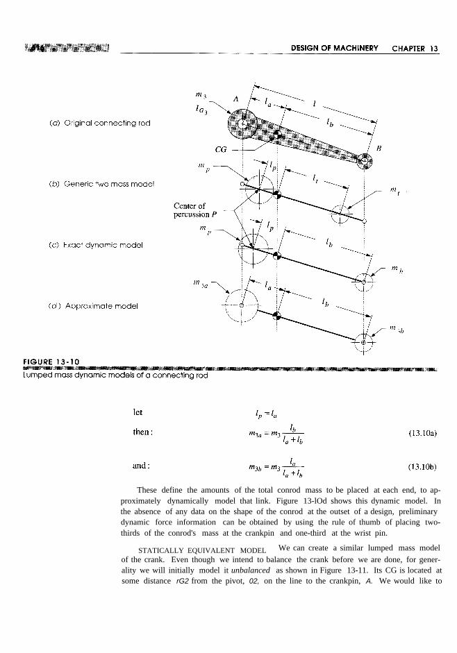
These define the amounts of the total conrod mass to be placed at each end, to ap-proximately dynamically model that link. Figure 13-lOd shows this dynamic model. Inthe absence of any data on the shape of the conrod at the outset of a design, preliminarydynamic force information can be obtained by using the rule of thumb of placing two-thirds of the conrod's mass at the crankpin and one-third at the wrist pin.
STATICALLY EQUIVALENT MODEL We can create a similar lumped mass modelof the crank. Even though we intend to balance the crank before we are done, for gener-ality we will initially model it unbalanced as shown in Figure 13-11. Its CG is located atsome distance rG2 from the pivot, 02, on the line to the crankpin, A. We would like to


Note that the gas force from equation 13.4 does not contribute to the shaking force.Only inertia forces and external forces are felt as shaking forces. The gas force is aninternal force which is cancelled within the mechanism. It acts equally and oppositelyon both the piston top and the cylinder head as shown in Figure 13-7 (p. 607).
Program ENGINE calculates the shaking force at constant 00, for any combination oflinkage parameters input to it. Figure 13-13 shows the shaking force plot for the sameunbalanced built-in example engine as shown in the acceleration plot (Figure l3-8c,p.611). The linkage orientation is the same as in Figure 13-12 (p. 618) with the x axishorizontal. The x component is larger than the y component due to the high accelerationof the piston. The forces are seen to be quite large despite this being a relatively small(0.4 liter per cylinder) engine running at moderate speed (3400 rpm). We will soon in-vestigate techniques to reduce or eliminate this shaking force from the engine. It is anundesirable feature which creates noise and vibration.
13.6 INERTIA AND SHAKING TORQUES
The inertia torque results from the action of the inertia forces at a moment arm. Theinertia force at point A in Figure 13-12 has two components, radial and tangential. Theradial component has no moment arm. The tangential component has a moment arm ofcrank radius r. If the crank 00 is constant, the mass at A will not contribute to inertiatorque. The inertia force at B has a nonzero component perpendicular to the cylinder wallexcept when the piston is at TDC or BDC. As we did for the gas torque, we can expressthe inertia torque in terms ofthe couple -Fi41, Fi41 whose forces act always perpendic-ular to the motion of the slider (neglecting friction), and the distance x, which is their in-stantaneous moment arm. The inertia torque is:

Program ENGINE calculates the inertia torque from equation B.15e. Figure 13-14shows a plot of the inertia torque for this built-in example engine. Note the dominanceof the second harmonic. The ideal magnitude for the inertia torque is zero, as it is para-sitic. Its average value is always zero, so it contributes nothing to the net driving torque.It merely creates large positive and negative oscillations in the total torque which in-crease vibration and roughness. We will soon investigate means to reduce or eliminatethis inertia and shaking torque in our engine designs. It is possible to cancel their ef-fects by proper arrangement of the cylinders in a multicylinder engine, as will be ex-plored in the next chapter.

13.8 FLYWHEELS
We saw in Section 11.11 (p. 548) that large oscillations in the torque-time function canbe significantly reduced by the addition of a flywheel to the system. The single-cylinderengine is a prime candidate for the use of a flywheel. The intermittent nature of its pow-er strokes makes one mandatory as it will store the kinetic energy needed to carry thepiston through the Otto cycle's exhaust, intake, and compression strokes during whichwork must be done on the system. Even the two-stroke engine needs a flywheel to drivethe piston up on the compression stroke.
The procedure for designing an engine flywheel is identical to that described in Sec-tion 11.11 for the fourbar linkage. The total torque function for one revolution of thecrank is integrated, pulse by pulse, with respect to its average value. These integrals rep-resent energy fluctuations in the system. The maximum change in energy under thetorque curve during one cycle is the amount needed to be stored in the flywheel. Equa-

tion 11.20c expresses this relationship. Program ENGINE does the numerical integrationof the total torque function and presents a table similar to the one shown in Figure 11-11(p. 551). These data and the designer's choice of a coefficient of fluctuation k (see equa-tion 11.19) are all that are needed to solve equations 11.20 and 11.21 for the requiredmoment of inertia of the flywheel.
The calculation must be done at some average crank 0). Since the typical engine op-erates over a wide range of speeds, some thought needs to be given to the most appropri-ate speed to use in the flywheel calculation. The flywheel's stored kinetic energy is pro-portional to co2 (see equation 11.17). Thus at high speeds a flywheel can have a smallmoment of inertia and still be effective. The slowest operating speed will require thelargest flywheel and should be the one used in the computation of required flywheel size.
Program ENGINE plots the flywheel-smoothed total torque for a user-supplied coef-ficient of fluctuation k. Figure 13-16 shows the smoothed torque functions for k = 0.05corresponding to the un smoothed ones in Figure 13-15. Note that the smoothed curvesshown for each engine speed are what would result with the flywheel size necessary toobtain that coefficient of fluctuation at that speed. In other words, the flywheel appliedto the 800-rpm engine is much larger than the one on the 6000-rpm engine, in these plots.Compare corresponding rows (speeds) between Figures 13-15 and 13-16 to see the ef-fect of the addition of a flywheel. But do not directly compare parts a, b, and c withinFigure 13-16 as to the amount of smoothing since the flywheel sizes used are different ateach operating speed.
An engine flywheel is usually designed as a flat disk, bolted to one end of the crank-shaft. One flywheel face is typically used for the clutch to run against. The clutch is afriction device which allows disconnection of the engine from the drive train (the wheelsof a vehicle) when no output is desired. The engine can then remain running at idle speedwith the vehicle or output device stopped. When the clutch is engaged, all engine torqueis transmitted through it, by friction, to the output shaft.
13.9 PIN FORCES IN THESINGLE-CYLINDER ENGINE
In addition to calculating the overall effects on the ground plane of the dynamic forcespresent in the engine, we also need to know the magnitudes of the forces at the pin joints.These forces will dictate the design of the pins and the bearings at the joints. Though wewere able to lump the mass due to both conrod and piston, or conrod and crank, at pointsA and B for an overall analysis of the linkage's effects on the ground plane, we cannot doso for the pin force calculations. This is because the pins feel the effect of the conrodpulling on one "side" and the piston (or crank) pulling on the other "side" of the pin asshown in Figure 13-17. Thus we must separate the effects of the masses of the linksjoined by the pins.
We will calculate the effect of each component due to the various masses, and thegas force and then superpose them to obtain the complete pin force at each joint. Weneed a bookkeeping system to keep track of all these components. We have already usedsome subscripts for these forces, so we will retain them and add others. The resultantbearing loads have the following components:


Note that, unlike the inertia force in equation 13.14 (p. 619), which was unaffectedby the gas force, these pin forces are a function of the gas force as well as of the -maforces. Engines with larger piston diameters will experience greater pin forces as a re-sult of the explosion pressure acting on their larger piston area.
Program ENGINE calculates the pin forces on all joints using equations 13.20 to13.23. Figure 13-21 shows the wrist-pin force on the same unbalanced engine exampleas shown in previous figures, for three engine speeds. The "bow tie" loop is the inertiaforce and the "teardrop" loop is the gas force portion of the force curve. An interestingtrade-off occurs between the gas force components and the inertia force components ofthe pin forces. At a low speed of 800 rpm (Figure l3-2la), the gas force dominates asthe inertia forces are negligible at small co. The peak wrist-pin force is then about 4200lb. At high speed (6000 rpm), the inertia components dominate and the peak force isabout 4500 lb (Figure 13-2lc). But at a midrange speed (3400 rpm), the inertia forcecancels some of the gas force and the peak force is only about 3200 lb (Figure 13-2lb).These plots show that the pin forces can be quite large even in a moderately sized (0.4liter/cylinder) engine. The pins, links, and bearings all have to be designed to withstandhundreds of millions of cycles of these reversing forces without failure.
Figure 13-22 shows further evidence of the interaction of the gas forces and inertiaforces on the crankpin and the wrist pin. Figures 13-22a and 13-22c show the variationin the inertia force component on the crankpin and wrist pin, respectively, over one full


revolution of the crank as the engine speed is increased from idle to redline. Figure13-22b and d show the variation in the total force on the same respective pins with boththe inertia and gas force components included. These two plots show only the first 900
of crank revolution where the gas force in a four-stroke cylinder occurs. Note that thegas force and inertia force components counteract one another resulting in one particu-lar speed where the total pin force is a minimum during the power stroke. This is thesame phenomenon as seen in Figure 13-21.
13.10 BALANCING THESINGLE-CYLINDER ENGINE
The derivations and figures in the preceding sections have shown that significant forcesare developed both on the pivot pins and on the ground plane due to the gas forces andthe inertia and shaking forces. Balancing will not have any effect on the gas forces,which are internal, but it can have a dramatic effect on the inertia and shaking forces.The main pin force can be reduced, but the crankpin and wrist pin forces will be unaf-fected by any crankshaft balancing done. Figure 13-13 (p. 620) shows the unbalancedshaking force as felt on the ground plane of our OA-liter-per-cylinder example enginefrom program ENGINE. It is about 9700 Ib even at the moderate speed of 3400 rpm. At6000 rpm it increases to over 30 000 lb. The methods of Chapter 12 can be applied to thismechanism to balance the members in pure rotation and reduce these large shaking forces.
Figure 13-23a shows the dynamic model of our slider-crank with the conrod masslumped at both crankpin A and wrist pin B. We can consider this single-cylinder engineto be a single-plane device, thus suitable for static balancing (see Section 13.1). It isstraightforward to statically balance the crank. We need a balance mass at some radius,1800 from the lumped mass at point A whose mr product is equal to the product of themass at A and its radius r. Applying equation 13.2 to this simple problem we get:
Any combination of mass and radius which gives this product, placed at 1800 frompoint A will balance the crank. For simplicity of example, we will use a balance radiusequal to r. Then a mass equal to mA placed at A ' will exactly balance the rotating mass-es. The CG ofthe crank will then be at the fixed pivot 02 as shown in Figure 13-23a. Ina real crankshaft, actually placing the counterweight at this large a radius would notwork. The balance mass has to be kept close to the centerline to clear the piston at BDC.Figure 13-2c shows the shape of typical crankshaft counterweights.
Figure 13-24a shows the shaking force from the same engine as in Figure 13-13 af-ter the crank has been exactly balanced in this manner. The Y component of the shakingforce has been reduced to zero and the x component to about 3300 Ib at 3400 rpm. Thisis a factor of three reduction over the unbalanced engine. Note that the only source of Ydirected inertia force is the rotating mass at point A of Figure 13-23 (see equations 13.14,p. 619). What remains after balancing the rotating mass is the force due to the accelera-tion of the piston and conrod masses at point B of Figure 13-23 which are in linear trans-lation along the X axis, as shown by the inertia force -mBaB at point B in that figure.
To completely eliminate this reciprocating unbalanced shaking force would requirethe introduction of another reciprocating mass, which oscillates 1800 out of phase withthe piston. Adding a second piston and cylinder, properly arranged, can accomplish this.
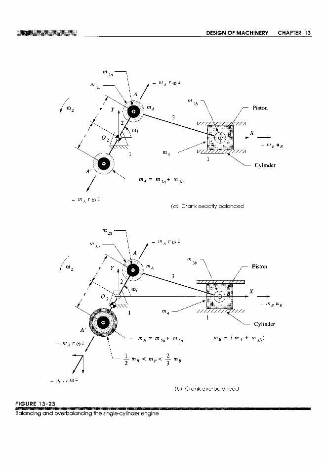


14.0 INTRODUCTION
The previous chapter discussed the design of the slider-crank mechanism as used in thesingle-cylinder internal combustion engine and piston pumps. We will now extend thedesign to multicylinder configurations. Some of the problems with shaking forces andtorques can be alleviated by proper combination of multiple slider-crank linkages on acommon crankshaft. Program ENGINE, included with this text, will calculate the equa-tions derived in this chapter and allow the student to exercise many variations of an en-gine design in a short time. Some examples are provided as disk files to be read into theprogram. These are noted in the text. The student is encouraged to investigate these ex-amples with program ENGINE in order to develop an understanding of and insight to thesubtleties of this topic. A user manual for program ENGINE is provided in Appendix Awhich can be read or referred to out of sequence, with no loss in continuity, in order togain familiarity with the program's operation.
As with the single-cylinder case, we will not address the thermodynamic aspects ofthe internal combustion engine beyond the definition of the combustion forces necessaryto drive the device presented in the previous chapter. We will concentrate on the engine'skinematic and mechanical dynamics aspects. It is not our intention to make an "enginedesigner" of the student so much as to apply dynamic principles to a realistic designproblem of general interest and also to convey the complexity and fascination involvedin the design of a more complicated dynamic device than the single-cylinder engine.
639


14.1 MUlTICYLINDER ENGINE DESIGNS
Multicylinder engines are designed in a wide variety of configurations from the simpleinline arrangement to vee, opposed, and radial arrangements some of which are shownin Figure 14-1. These arrangements may use any of the stroke cycles discussed in Chap-ter 13, Clerk, Otto, or Diesel.
IN LINE ENGINES The most common and simplest arrangement is an inline enginewith its cylinders all in a common plane as shown in Figure 14-2. Two-,* three-,* four,five, and six-cylinder inUne engines are in common use. Each cylinder will have its in-dividual slider-crank mechanism consisting of a crank, conrad, and piston. The cranksare formed together in a common crankshaft as shown in Figure 14-3. Each cylinder'scrank on the crankshaft is referred to as a crank throw. These crank throws will be ar-ranged with some phase angle relationship one to the other, in order to stagger the mo-tions of the pistons in time. It should be apparent from the discussion of shaking forcesand balancing in the previous chapter that we would like to have pistons moving in op-posite directions to one another at the same time in order to cancel the reciprocating in-ertial forces. The optimum phase angle relationships between the crank throws will dif-fer depending on the number of cylinders and the stroke cycle of the engine. There willusually be one (or a small number at) viable crank throw arrangements for a given en-gine configuration to accomplish this goal. The engine in Figure 14-2 is a four-strokecycle, four-cylinder, inline engine with its crank throws at 0, 180, 180, and 0° phaseangles which we will soon see are optimum for this engine. Figure 14-3 shows the crank-shaft, connecting rods and pistons for the same design of engine as in Figure 14-2.
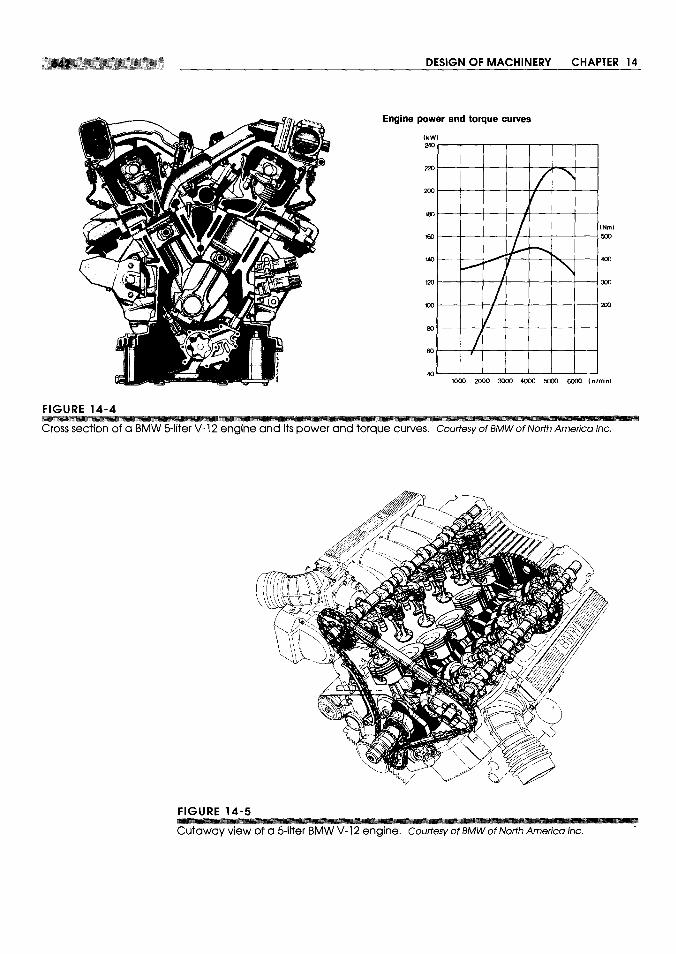

VEE ENGINES in two-, * four-, * six-, eight-, ten-, t and twelve-cylinder+ versionsare produced, with vee six and vee eight being the most common configurations. Figure14-4 shows a cross section and Figure 14-5 a cutaway of a 60° vee -twelve engine. Veeengines can be thought of as two inline engines grafted together onto a common crank-shaft. The two "inline" portions, or banks, are arranged with some vee angle betweenthem. Figure 14-ld shows a vee-eight engine. Its crank throws are at 0,90,270, and180° respectively. A vee eight's vee angle is 90°. The geometric arrangements of thecrankshaft (phase angles) and cylinders (vee angle) have a significant effect on the dy-namic condition of the engine. We will soon explore these relationships in detail.
OPPOSED ENGINES are essentially vee engines with a vee angle of 180°. The pis-tons in each bank are on opposite sides of the crankshaft as shown in Figure 14-6. Thisarrangement promotes cancellation of inertial forces and is popular in aircraft engines. §It has also been used in some automotive applications. II
RADIAL ENGINES have their cylinders arranged radially around the crankshaft innearly a common plane. These were common on World War II vintage aircraft as theyallowed large displacements, and thus high power, in a compact form whose shape waswell suited to that of an airplane. Typically air cooled, the cylinder arrangement allowedgood exposure of all cylinders to the airstream. Large versions had multiple rows of ra-dial cylinders, rotationally staggered to allow cooling air to reach the back rows. Thegas turbine jet engine has rendered these radial aircraft engines obsolete.
ROTARY ENGINES were an interesting variant on the aircraft radial engine. Sim-ilar in appearance and cylinder arrangement to the radial engine, the anomaly was thatthe crankshaft was the stationary ground plane. The propeller was attached to the crank-case (block) which rotated around the crankshaft! It is a kinematic inversion of the radi-al engine. At least it didn't need a flywheel.
Many other configurations of engines have been tried over the century of develop-ment of this ubiquitous device. The bibliography at the end of this chapter contains sev-eral references which describe other engine designs, the usual, unusual, and exotic. Wewill begin our detailed exploration of multicylinder engine design with the simplest con-figuration, the inline engine, and then progress to the vee and opposed versions.

We must establish some convention for the measurement of these phase angleswhich will be:
1 The first (front) cylinder will be number 1 and its phase angle will always be zero.It is the reference cylinder for all others.
2 The phase angles of all other cylinders will be measured with respect to the crankthrow for cylinder 1.
3 Phase angles are measured internal to the crankshaft, that is, with respect to a rotat-ing coordinate system embedded in the first crank throw.
4 Cylinders will be numbered consecutively from front to back of the engine.
The phase angles are defined in a crank phase diagram as shown in Figure 14-7for a four-cylinder, inline engine. Figure l4-7a shows the crankshaft with the throwsnumbered clockwise around the axis. The shaft is rotating counterclockwise. The pis-tons are oscillating horizontally in this diagram, along the x axis. Cylinder 1 is shownwith its piston at top dead center (TDC). Taking that position as the starting point for theabscissas (thus time zero) in Figure 14-7b, we plot the velocity of each piston for tworevolutions of the crank (to accommodate one complete four-stroke cycle). Piston 2 ar-rives at TDC 90° after piston 1 has left. Thus we say that cylinder 2 lags cylinder 1 by90 degrees. By convention a lagging event is defined as having a negative phase angle,shown by the clockwise numbering of the crank throws. The velocity plots clearly showthat each cylinder arrives at TDC (zero velocity) 90° later than the one before it. Nega-tive velocity on the plots in Figure l4-7b indicates piston motion to the left (down stroke)in Figure l4-7a; positive velocity indicates motion to the right (up stroke).
For the discussion in this chapter we will assume counterclockwise rotation of allcrankshafts, and all phase angles will thus be negative. We will, however, omit the neg-ative signs on the listings of phase angles with the understanding that they follow thisconvention.
Figure 14-7 shows the timing of events in the cycle and is a necessary and usefulaid in defining our crankshaft design. However, it is not necessary to go to the trouble ofdrawing the correct sinusoidal shapes of the velocity plots to obtain the needed informa-tion. All that is needed is a schematic indication of the relative positions within the cy-


11.11 CONTROLLING INPUT TORQUE-flYWHEElS
The typically large variation in accelerations within a mechanism can cause significantoscillations in the torque required to drive it at a constant or near constant speed. Thepeak torques needed may be so high as to require an overly large motor to deliver them.However, the average torque over the cycle, due mainly to losses and external work done,may often be much smaller than the peak torque. We would like to provide some meansto smooth out these oscillations in torque during the cycle. This will allow us to size themotor to deliver the average torque rather than the peak torque. One convenient and rel-atively inexpensive means to this end is the addition of a flywheel to the system.
TORQUE VARIATION Figure 11-8 shows the variation in the input torque for acrank-rocker fourbar linkage over one full revolution of the drive crank. It is running ata constant angular velocity of 50 rad/sec. The torque varies a great deal within one cy-cle of the mechanism, going from a positive peak of 341.7 Ib-in to a negative peak of-166.41b-in. The average value of this torque over the cycle is only 70.21b-in, beingdue to the external work done plus losses. This linkage has only a 12-lb external forceapplied to link 3 at the CG and a 25 Ib-in external torque applied to link 4. These smallexternal loads cannot account for the large variation in input torque required to maintainconstant crank speed. What then is the explanation? The large variations in torque areevidence of the kinetic energy that is stored in the links as they move. We can think ofthe positive pulses of torque as representing energy delivered by the driver (motor) andstored temporarily in the moving links, and the negative pulses of torque as energy at-tempting to return from the links to the driver. Unfortunately most motors are designedto deliver energy but not to take it back. Thus the "returned energy" has no place to go.
Figure 11-9 shows the speed torque characteristic of a permanent magnet (PM) DCelectric motor. Other types of motors will have differently shaped functions that relatemotor speed to torque as shown in Figure 2-32 and 2-33 (pp. 62-63), but all drivers


average, the sum of positive area above an average line is equal to the sum of negative areabelow that line.) The integration limits in equation 11.18 are from the shaft angle 8 at whichthe shaft (j)is a minimum to the shaft angle 8 at which (j) is a maximum.
3 The minimum (j)will occur after the maximum positive energy has been delivered from themotor to the load, i.e., at a point (8) where the summation of positive energy (area) in thetorque pulses is at its largest positive value.
4 The maximum (j)will occur after the maximum negative energy has been returned to the load,i.e., at a point (8) where the summation of energy (area) in the torque pulses is at its largestnegative value.
5 To find these locations in 8 corresponding to the maximum and minimum (j)'s and thus findthe amount of energy needed to be stored in the flywheel, we need to numerically integrateeach pulse of this function from crossover to crossover with the average line. The crossoverpoints in Figure 11-11 have been labeled A, B, C, and D. (Program FOURBARdoes this inte-gration for you numerically, using a trapezoidal rule.)
6 The FOURBARprogram prints the table of areas shown in Figure 11-11. The positive andnegative pulses are separately integrated as described above. Reference to the plot of thetorque function will indicate whether a positive or negative pulse is the first encountered ina particular case. The first pulse in this example is a positive one.
7 The remaining task is to accumulate these pulse areas beginning at an arbitrary crossover (inthis case point A) and proceeding pulse by pulse across the cycle. Table 11-1 shows this pro-cess and the result.
8 Note in Table 11-1 that the minimum shaft speed occurs after the largest accumulated posi-tive energy pulse (+200.73 in-lb) has been delivered from the driveshaft to the system. Thisdelivery of energy slows the motor down. The maximum shaft speed occurs after the largestaccumulated negative energy pulse (-60.32 in-lb) has been received back from the systemby the driveshaft. This return of stored energy will speed up the motor. The total energyvariation is the algebraic difference between these two extreme values, which in this exam-ple is -261.05 in-lb. This negative energy coming out of the system needs to be absorbed bythe flywheel and then returned to the system during each cycle to smooth the variations inshaft speed.


the torque curve (see Table 11-1, p. 552) and the average shaft (i) to compute the neededsystem Is. The physical flywheel's mass moment of inertia If is then set equal to the re-quired system Is. But if the moments of inertia of the other rotating elements on the samedriveshaft (such as the motor) are known, the physical flywheel's required If can be re-duced by those amounts.
The most efficient flywheel design in terms of maximizing Iffor minimum materialused is one in which the mass is concentrated in its rim and its hub is supported onspokes, like a carriage wheel. This puts the majority of the mass at the largest radiuspossible and minimizes the weight for a given If Even if a flat, solid circular disk fly-wheel design is chosen, either for simplicity of manufacture or to obtain a flat surfacefor other functions (such as an automobile clutch), the design should be done with an eyeto reducing weight and thus cost. Since in general, I = m,.2, a thin disk of large diame-ter will need fewer pounds of material to obtain a given I than will a thicker disk of small-er diameter. Dense materials such as cast iron and steel are the obvious choices for a fly-wheel. Aluminum is seldom used. Though many metals (lead, gold, silver, platinum) aremore dense than iron and steel, one can seldom get the accounting department's approv-al to use them in a flywheel.
Figure 11-12 shows the change in the input torque T12 for the linkage in Figure 11-8after the addition of a flywheel sized to provide a coefficient of fluctuation of 0.05. Theoscillation in torque about the unchanged average value is now 5%, much less than whatit was without the flywheel. A much smaller horsepower motor can now be used becausethe flywheel is available to absorb the energy returned from the linkage during its cycle.
11.12 A LINKAGE FORCE TRANSMISSION INDEX
The transmission angle was introduced in Chapter 2 and used in subsequent chapters asan index of merit to predict the kinematic behavior of a linkage. A too-small transmis-sion angle predicts problems with motion and force transmission in a fourbar linkage.Unfortunately, the transmission angle has limited application. It is only useful for four-bar linkages and then only when the input and output torques are applied to links that are

pivoted to ground (i.e., the crank and rocker). When external forces are applied to thecoupler link, the transmission angle tells nothing about the linkage's behavior.
Holte and Chase [1] define a joint-force index (IPl) which is useful as an indicatorof any linkage's ability to smoothly transmit energy regardless of where the loads areapplied on the linkage. It is applicable to higher-order linkages as well as to the fourbarlinkage. The IPI at any instantaneous position is defined as the ratio of the maximumstatic force in any joint of the mechanism to the applied external load. If the externalload is a force, then it is:
The F ij are calculated from a static force analysis of the linkage. Dynamic forcescan be much greater than static forces if speeds are high. However, if this static forcetransmission index indicates a problem in the absence of any dynamic forces, then thesituation will obviously be worse at speed. The largest joint force at each position is usedrather than a composite or average value on the assumption that high friction in anyonejoint is sufficient to hamper linkage performance regardless of the forces at other joints.
Equation 11.23a is dimensionless and so can be used to compare linkages of differ-ent design and geometry. Equation 11.23b has dimensions of reciprocal length, so cau-tion must be exercised when comparing designs when the external load is a torque. Thenthe units used in any comparison must be the same, and the compared linkages shouldbe similar in size.
Equations 11.23 apply to anyone instantaneous position of the linkage. As with thetransmission angle, this index must be evaluated for all positions of the linkage over itsexpected range of motion and the largest value of that set found. The peak force maymove from pin to pin as the linkage rotates. If the external loads vary with linkage posi-tion, they can be accounted for in the calculation.
Holte and Chase suggest that the IPI be kept below a value of about 2 for linkageswhose output is a force. Larger values may be tolerable especially if the joints are de-signed with good bearings that are able to handle the higher loads.
There are some linkage positions in which the IPI can become infinite or indetermi-nate as when the linkage reaches an immovable position, defined as the input link or in-put joint being inactive. This is equivalent to a stationary configuration as described inearlier chapters provided that the input joint is inactive in the particular stationary con-figuration. These positions need to be identified and avoided in any event, independentof the determination of any index of merit. In some cases the mechanism may be im-movable but still capable of supporting a load. See reference [1] for more detailed infor-mation on these special cases.

11.13 PRACTICAL CONSIDERATIONS
This chapter has presented some approaches to the computation of dynamic forces inmoving machinery. The newtonian approach gives the most information and is neces-sary in order to obtain the forces at all pin joints so that stress analyses of the memberscan be done. Its application is really quite straightforward, requiring only the creationof correct free-body diagrams for each member and the application of the two simplevector equations which express Newton's second law to each free-body. Once theseequations are expanded for each member in the system and placed in standard matrixform, their solution (with a computer) is a trivial task.
The real work in designing these mechanisms comes in the determination of theshapes and sizes of the members. In addition to the kinematic data, the force computa-tion requires only the masses, CG locations, and mass moments of inertia versus thoseCGs for its completion. These three geometric parameters completely characterize themember for dynamic modelling purposes. Even if the link shapes and materials are com-pletely defined at the outset of the force analysis process (as with the redesign of an ex-isting system), it is a tedious exercise to calculate the dynamic properties of complicatedshapes. Current solids modelling CAD systems make this step easy by computing theseparameters automatically for any part designed within them.
If, however, you are starting from scratch with your design, the blank-paper syn-drome will inevitably rear its ugly head. A first approximation of link shapes and selec-tion of materials must be made in order to create the dynamic parameters needed for a"first pass" force analysis. A stress analysis of those parts, based on the calculated dy-namic forces, will invariably find problems that require changes to the part shapes, thusrequiring recalculation of the dynamic properties and recomputation of the dynamic forc-es and stresses. This process will have to be repeated in circular fashion (iteration-seeChapter 1, p. 8) until an acceptable design is reached. The advantages of using a com-puter to do these repetitive calculations is obvious and cannot be overstressed. An equa-tion solver program such as TKSolver or Mathcad will be a useful aid in this process byreducing the amount of computer programming necessary.
Students with no design experience are often not sure how to approach this processof designing parts for dynamic applications. The following suggestions are offered toget you started. As you gain experience, you will develop your own approach.
It is often useful to create complex shapes from a combination of simple shapes, atleast for first approximation dynamic models. For example, a link could be consideredto be made up of a hollow cylinder at each pivot end, connected by a rectangular prismalong the line of centers. It is easy to calculate the dynamic parameters for each of thesesimple shapes and then combine them. The steps would be as follows (repeated for eachlink):
1 Calculate the volume, mass, CG location, and mass moments of inertia with respectto the local CG of each separate part of your built-up link. In our example link theseparts would be the two hollow cylinders and the rectangular prism.
2 Find the location of the composite CG of the assembly of the parts into the link bythe method shown in Section 11.4 (p. 531) and equation 11.3 (p. 524). See also Fig-ure 11-2 (p. 526).


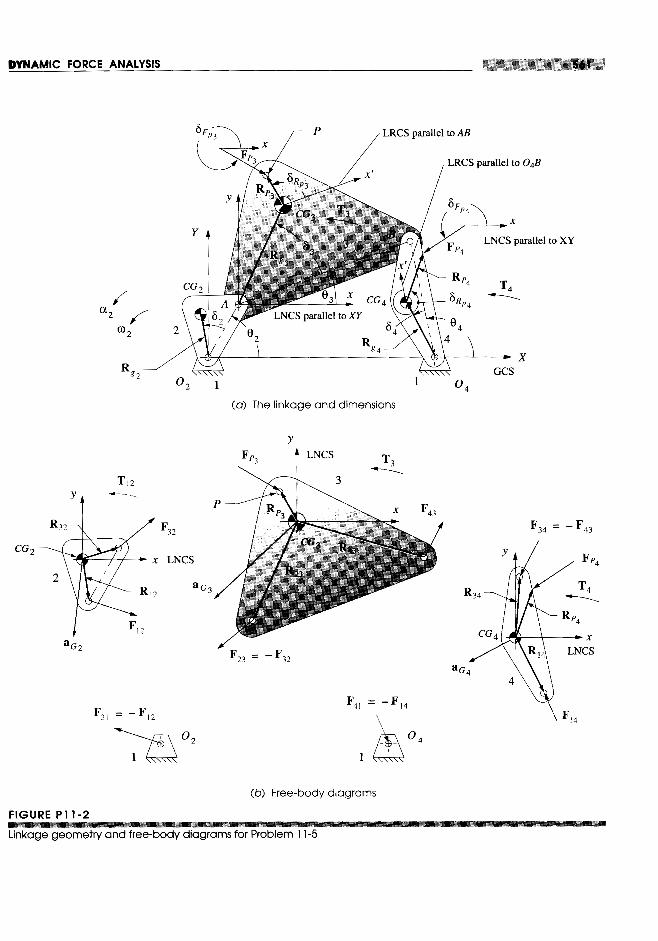


secZ. There is a vertical force at P of F = 500 N. Find all pin forces and the torqueneeded to drive the crank at this instant.
*t:J:11-12 Figure PII-5b shows a fourbar linkage and its dimensions in meters. The steel crank,coupler, and rocker have uniform cross sections of 50 mm diameter. In the instanta-neous position shown, the crank OzA has 0) = -10 rad/sec and a = 10 rad/sec2. Thereis a horizontal force at P of F = 300 N. Find all pin forces and the torque needed todrive the crank at this instant.
*t:J:11-13 Figure PII-6 shows a water jet loom laybar drive mechanism driven by a pair ofGrashof crank rocker fourbar linkages. The crank rotates at 500 rpm. The laybar iscarried between the coupler-rocker joints of the two linkages at their respectiveinstant centers h,4. The combined weight of the reed and laybar is 29 lb. A 540-lbbeat-up force from the cloth is applied to the reed as shown. The steel links have a 2X I in uniform cross section. Find the forces on the pins for one revolution of thecrank. Find the torque-time function required to drive the system.
tll-14 Figure PII-7 shows a crimping tool. Find the force Fhandneeded to generate a 2000-Ib Fcrimp' Find the pin forces. What is this linkage's joint force transmission index(IFI) in this position?
t§ 11-15 Figure P 11-8 shows a walking beam conveyor mechanism that operates at slow speed(25 rpm). The boxes being pushed each weigh 50 lb. Determine the pin forces in thelinkage and the torque required to drive the mechanism through one revolution.Neglect the masses of the links.
t§ 11-16 Figure PII-9 shows a surface grinder table drive that operates at 120 rpm. The crankradius is 22 mm, the coupler is 157 mm, and its offset is 40 mm. The mass of tableand workpiece combined is 50 kg. Find the pin forces, slider side loads, and drivingtorque over one revolution.
t§1l-17 Figure Pll-1O shows a power hacksaw that operates at 50 rpm. The crank is 75 mm,the coupler is 170 mm, and its offset is 45 mm. Find the pin forces, slider side loads,and driving torque over one revolution for a cutting force of 250 N in the forwarddirection and 50 N during the return stroke.

t§11-18 Figure Pll-ll shows a paper roll off-loading station. The paper rolls have a 0.9-mOD, 0.22-m ID, are 3.23 m long, and have a density of 984 kg/m3. The forks thatsupport the roll are 1.2 m long. The motion is slow so inertial loading can beneglected. Find the force required of the air cylinder to rotate the roll through 90°.
t 11-19 Derive an expression for the relationship between flywheel mass and the dimension-less parameter radius/thickness (r/t) for a solid disk flywheel of moment of inertia f.Plot this function for an arbitrary value of f and determine the optimum r/t ratio tominimize flywheel weight for that f.


The following problem statement applies to all the projects listed.These larger-scale project statements deliberately lack detail and structure and areloosely defined. Thus, they are similar to the kind of "identification of need " or problemstatement commonly encountered in engineering practice. It is left to the student to struc-ture the problem through background research and to create a clear goal statement andset of performance specifications before attempting to design a solution. This designprocess is spelled out in Chapter 1 and should befollowed in all of these examples. Allresults should be documented in a professional engineering report. See the Bibliogra-phy in Chapter 1 for references on report writing.
Some of these project problems are based on the kinematic design projects in Chap-ter 3. Those kinematic devices can now be designed more realistically with considerationof the dynamic forces that they generate. The strategy in most of the following projectproblems is to keep the dynamic pin forces and thus the shaking forces to a minimum andalso keep the input torque-time curve as smooth as possible to minimize power require-ments. All these problems can be solved with a pin-jointed fourbar linkage. This factwill allow you to use program FOURBAR to do the kinematic and dynamic computationson a large number and variety of designs in a short time. There are infinities of viablesolutions to these problems. Iterate to find the best one! All links must be designed indetail as to their geometry (mass, moment of inertia, etc.). An equation solver such asMathcad or TKSolver will be useful here. Determine all pin forces, shaking force, shak-ing torque, and input horsepower required for your designs.
Pll-l Project P3-1 stated that:
The tennis coach needs a better tennis ball server for practice. This device must fire asequence of standard tennis balls from one side of a standard tennis court over the netsuch that they land and bounce within each of the three court areas defined by thecourt's white lines. The order and frequency of a ball's landing in anyone of thethree court areas must be random. The device should operate automatically andunattended except for the refill of balls. It should be capable of firing 50 ballsbetween reloads. The timing of ball releases should vary. For simplicity, a motor-driven pin-jointed linkage design is preferred.
This project asks you to design such a device to be mounted upon a tripod stand of5-foot height. Design it, and the stand, for stability against tipover due to the shakingforces and shaking torques which should also be minimized in the design of yourlinkage. Minimize the input torque required.
PII-2 Project P3-9 stated that:
The "Save the Skeet" foundation has requested a more humane skeet launcher bedesigned. While they have not yet succeeded in passing legislation to prevent thewholesale slaughter of these little devils, they are concerned about the inhumaneaspects of the large accelerations imparted to the skeet as it is launched into the skyfor the sportsperson to shoot it down. The need is for a skeet launcher that willsmoothly accelerate the clay pigeon onto its desired trajectory.

Design a skeet launcher to be mounted upon a child's "little red wagon." Controlyour design parameters so as to minimize the shaking forces and torques so that thewagon will remain as nearly stationary as possible during the launch of the claypigeon.
Pl1-3 Project P3-10 stated that:
The coin-operated "kid bouncer" machines found outside supermarkets typicallyprovide a very unimaginative rocking motion to the occupant. There is a need for asuperior "bouncer" which will give more interesting motions while remaining safe forsmall children.
Design this device for mounting in the bed of a pickup truck. Keep the shakingforces to a minimum and the input torque-time curve as smooth as possible.
Pl1-4 Project P3-15 stated that:
NASA wants a zero-G machine for astronaut training. It must carry one person andprovide a negative l-g acceleration for as long as possible.Design this device and its mounting hardware to the ground plane minimizing thedynamic forces and driving torque.
Pl1-5 Project P3-16 stated that:
The Amusement Machine Co. Inc. wants a portable "WHIP" ride which will give twoor four passengers a thrilling but safe ride and which can be trailed behind a pickuptruck from one location to another.
Design this device and its mounting hardware to the truck bed minimizing thedynamic forces and driving torque.
P 11-6 Project P3-17 stated that:
The Air Force has requested a pilot training simulator which will give potential pilotsexposure to G forces similar to those they will experience in dogfight maneuvers.Design this device and its mounting hardware to the ground plane minimizing thedynamic forces and driving torque.
Pl1-7 Project P3-18 stated that:
Cheers needs a better "mechanical bull" simulator for their "yuppie" bar in Boston. Itmust give a thrilling "bucking bronco" ride but be safe.Design this device and its mounting hardware to the ground plane minimizing thedynamic forces and driving torque.
Pll-8 Gargantuan Motors Inc. is designing a new light military transport vehicle. Theircurrent windshield wiper linkage mechanism develops such high shaking forces whenrun at its highest speed that the engines are falling out! Design a superior windshieldwiper mechanism to sweep the 20-lb armored wiper blade through a 90° arc whileminimizing both input torque and shaking forces. The wind load on the blade,perpendicular to the windshield, is 50 lb. The coefficient of friction of the wiperblade on glass is 0.9.

PII-9 The Anny's latest helicopter gunship is to be fitted with the Gatling gun, which fires
50-mm-diameter, 2-cm-long spent uranium slugs at a rate of 10 rounds per second.
The reaction (recoil) force may upset the chopper's stability. A mechanism is needed
which can be mounted to the frame of the helicopter and which will provide a
synchronous shaking force, 1800 out of phase with the recoil force pulses, to
counteract the recoil of the gun. Design such a linkage and minimize its torque and
power drawn from the aircraft's engine. Total weight of your device should also beminimized.
Pll-1O Steel pilings are universally used as foundations for large buildings. These are often
driven into the ground by hammer blows from a "pile driver." In certain soils (sandy,
muddy) the piles can be "shaken" into the ground by attaching a "vibratory driver"
which imparts a vertical, dynamic shaking force at or near the natural frequency of
the pile-earth system. The pile can literally be made to "fall into the ground" under
optimal conditions. Design a fourbar linkage-based pile shaker mechanism which,
when its ground link is finnly attached to the top of a piling (supported from a crane
hook), will impart a dynamic shaking force that is predominantly directed along the
piling's long, vertical axis. Operating speed should be in the vicinity of the naturalfrequency of the pile-earth system.
Pll-ll Paint can shaker mechanisms are common in paint and hardware stores. While they
do a good job of mixing the paint, they are also noisy and transmit their vibrations to
the shelves and counters. A better design of the paint can shaker is possible using a
balanced fourbar linkage. Design such a portable device to sit on the floor (not
bolted down) and minimize the shaking forces and vibrations while still effectivelymixing the paint.
PII-12 Convertible automobiles are once again popular. While offering the pleasure of
open-air motoring, they offer little protection to the occupants in a rollover accident.
Pennanent roll bars are ugly and detract from the open feeling of a true convertible.
An automatically deployable roll bar mechanism is needed that will be out of sight
until needed. In the event that sensors in the vehicle detect an imminent rollover, the
mechanism should deploy within 250 ms. Design a collapsible/deployable roll barmechanism to retrofit to the convertible of your choice.

12.0 INTRODUCTIONAny link or member that is in pure rotation can, theoretically, be perfectly balanced toeliminate all shaking forces and shaking moments. It is accepted design practice to bal-ance all rotating members in a machine unless shaking forces are desired (as in a vibrat-ing shaker mechanism, for example). A rotating member can be balanced either statical-ly or dynamically. Static balance is a subset of dynamic balance. To achieve completebalance requires that dynamic balancing be done. In some cases, static balancing can bean acceptable substitute for dynamic balancing and is generally easier to do.
Rotating parts can, and generally should, be designed to be inherently balanced bytheir geometry. However, the vagaries of production tolerances guarantee that there willstill be some small unbalance in each part. Thus a balancing procedure will have to beapplied to each part after manufacture. The amount and location of any imbalance canbe measured quite accurately and compensated for by adding or removing material in the
correct locations.In this chapter we will investigate the mathematics of determining and designing a
state of static and dynamic balance in rotating elements and also in mechanisms havingcomplex motion, such as the fourbar linkage. The methods and equipment used to mea-

sure and correct imbalance in manufactured assemblies will also be discussed. It is quiteconvenient to use the method of d' Alembert (see Section 10.12, p. 513) when discussingrotating imbalance, applying inertia forces to the rotating elements, so we will do that.
12.1 STATIC BALANCE
Despite its name, static balance does apply to things in motion. The unbalanced forcesof concern are due to the accelerations of masses in the system. The requirement forstatic balance is simply that the sum of all forces on the moving system (includingd'Alembert inertial forces) must be zero.
This, of course, is simply a restatement of Newton's law as discussed in Section 10.1 (p. 491).
Another name for static balance is single-plane balance, which means that themasses which are generating the inertia forces are in, or nearly in, the same plane. It isessentially a two-dimensional problem. Some examples of common devices which meetthis criterion, and thus can successfully be statically balanced, are: a single gear or pul-ley on a shaft, a bicycle or motorcycle tire and wheel, a thin flywheel, an airplane pro-peller, an individual turbine blade-wheel (but not the entire turbine). The common de-nominator among these devices is that they are all short in the axial direction comparedto the radial direction, and thus can be considered to exist in a single plane. An automo-bile tire and wheel is only marginally suited to static balancing as it is reasonably thickin the axial direction compared to its diameter. Despite this fact, auto tires are sometimesstatically balanced. More often they are dynamically balanced and will be discussedunder that topic.
Figure l2-la shows a link in the shape of a vee which is part of a linkage. We wantto statically balance it. We can model this link dynamically as two point masses ml andm2 concentrated at the local CGs of each "leg" of the link as shown in Figure l2-lb.These point masses each have a mass equal to that of the "leg" they replace and are sup-ported on massless rods at the position (R1 or R2) ofthat leg's CG. We can solve for therequired amount and location of a third "balance mass" mb to be added to the system atsome location Rb in order to satisfy equation 12.1.
Assume that the system is rotating at some constant angular velocity 00. The accel-erations of the masses will then be strictly centripetal (toward the center) , and the iner-tia forces will be centrifugal (away from the center) as shown in Figure 12-1. Since thesystem is rotating, the figure shows a "freeze-frame" image of it. The position at whichwe "stop the action" for the purpose of drawing the picture and doing the calculations isboth arbitrary and irrelevant to the computation. We will set up a coordinate system withits origin at the center of rotation and resolve the inertial forces into components in thatsystem. Writing vector equation 12.1 for this system we get:
Note that the only forces acting on this system are the inertia forces. For balancing,it does not matter what external forces may be acting on the system. External forcescannot be balanced by making any changes to the system's internal geometry. Note thatthe ro2 terms cancel. For balancing, it also does not matter how fast the system is rotat-
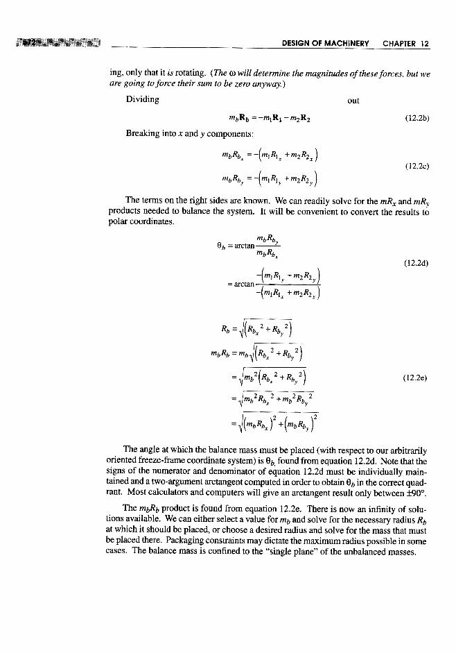


These moments act in planes that include the axis of rotation of the assembly suchas planes XZ and YZ in Figure 12-2. The moment's vector direction, or axis, is perpen-dicular to the assembly's axis of rotation.
Any rotating object or assembly which is relatively long in the axial direction com-pared to the radial direction requires dynamic balancing for complete balance. It is pos-sible for an object to be statically balanced but not be dynamically balanced. Considerthe assembly in Figure 12-2. TWo equal masses are at identical radii, 1800 apart rota-tionally, but separated along the shaft length. A summation of -ma forces due to theirrotation will be always zero. However, in the side view, their inertia forces form a cou-ple which rotates with the masses about the shaft. This rocking couple causes a momenton the ground plane, alternately lifting and dropping the left and right ends of the shaft.
Some examples of devices which require dynamic balancing are: rollers, crank-shafts, camshafts, axles, clusters of multiple gears, motor rotors, turbines, propellershafts. The common denominator among these devices is that their mass may be uneven-ly distributed both rotationally around their axis and also longitudinally along their axis.
To correct dynamic imbalance requires either adding or removing the right amountof mass at the proper angular locations in two correction planes separated by some dis-tance along the shaft. This will create the necessary counter forces to statically balancethe system and also provide a counter couple to cancel the unbalanced moment. Whenan automobile tire and wheel is dynamically balanced, the two correction planes are theinner and outer edges of the wheel rim. Correction weights are added at the proper loca-tions in each of these correction planes based on a measurement of the dynamic forcesgenerated by the unbalanced, spinning wheel.


So, when the design is still on the drawing board, these simple analysis techniquescan be used to determine the necessary sizes and locations of balance masses for anyassembly in pure rotation for which the mass distribution is defined. This two-planebalance method can be used to dynamically balance any system in pure rotation, and allsuch systems should be balanced unless the purpose of the device is to create shakingforces or moments.
12.3 BALANCING LINKAGES
Many methods have been devised to balance linkages. Some achieve a complete bal-ance of one dynamic factor, such as shaking force, at the expense of other factors suchas shaking moment or driving torque. Others seek an optimum arrangement that collec-tively minimizes (but does not zero) shaking forces, moments, and torques for a bestcompromise. Lowen and Berkof, [1] and Lowen, Tepper, and Berkof [2] give compre-hensive reviews of the literature on this subject up to 1983. Additional work has beendone on the problem since that time, some of which is noted in the references at the endof this chapter.
Complete balance of any mechanism can be obtained by creating a second "mirrorimage" mechanism connected to it so as to cancel all dynamic forces and moments.Certain configurations of multicylinder internal combustion engines do this. The pistonsand cranks of some cylinders cancel the inertial effects of others. We will explore theseengine mechanisms in Chapter 14. However, this approach is expensive and is only jus-tified if the added mechanism serves some second purpose such as increasing power, asin the case of additional cylinders in an engine. Adding a "dummy" mechanism whoseonly purpose is to cancel dynamic effects is seldom economically justifiable.
Most practical linkage balancing schemes seek to minimize or eliminate one or moreof the dynamic effects (forces, moments, torques) by redistributing the mass of the ex-isting links. This typically involves adding counterweights and/or changing the shapesof links to relocate their CGs. More elaborate schemes add geared counterweights tosome links in addition to redistributing their mass. As with any design endeavor, thereare trade-offs. For example, elimination of shaking forces usually increases the shakingmoment and driving torque. We can only present a few approaches to this problem inthe space available. The reader is directed to the literature for information on other methods.

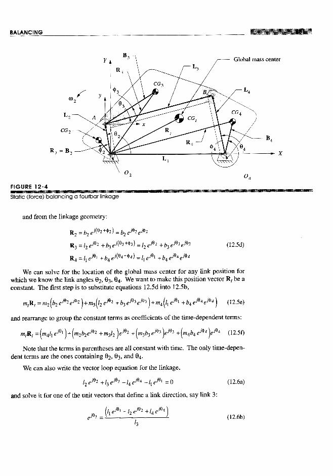

We now have two equations involving three links. The parameters for anyone linkcan be assumed and the other two solved for. A linkage is typically first designed to sat-isfy the required motion and packaging constraints before this force balancing procedureis attempted. In that event, the link geometry and masses are already defined, at least ina preliminary way. A useful strategy is to leave the link 3 mass and CG location as orig-inally designed and calculate the necessary masses and CG locations of links 2 and 4 tosatisfy these conditions for balanced forces. Links 2 and 4 are in pure rotation, so it isstraightforward to add counterweights to them in order to move their CGs to the neces-sary locations. With this approach, the right sides of equations 12.8b are reducible tonumbers for a designed linkage. We want to solve for the mass radius products m2b2 andm4b4 and also for the angular locations of the CGs within the links. Note that the angles<1>2 and <1>4 in equation 12.8 are measured with respect to the lines of centers of their re-spective links.
Equations 12.8b are vector equations. Substitute the Euler identity (equation 4.4a,p. 155) to separate into real and imaginary components, and solve for the x and y compo-nents of the mass-radius products.

These components of the mR product needed to force balance the linkage representthe entire amount needed. If links 2 and 4 are already designed with some individualunbalance (the CG not at pivot), then the existing mR product of the unbalanced link mustbe subtracted from that found in equations 12.8c and 12.8d in order to determine the sizeand location of additional counterweights to be added to those links. As we did with thebalance of rotating links, any combination of mass and radius that gives the desired prod-uct is acceptable. Use equations 12.2d and 12.2e to convert the cartesian mR products inequations 12.8c and 12.8d to polar coordinates in order to find the magnitude and angleof the counterweight's mR vector. Note that the angle of the mR vector for each link willbe referenced to that link's line of centers. Design the shape of the physical counter-weights to be put on the links as discussed in Section 12.1 (p. 571).
12.4 EFFECTOF BALANCING ON SHAKING AND PIN FORCES
Figure 12-5 shows a fourbar linkage* to which balance masses have been added in ac-cord with equations 12.8. Note the counterweights placed on links 2 and 4 at the calcu-lated locations for complete force balance. Figure 12-6a shows a polar plot of the shak-ing forces of this linkage without the balance masses. The maximum is 462 Ib at 15°.Figure 12-6b shows the shaking forces after the balance masses are added. The shakingforces are reduced to essentially zero. The small residual forces seen in Figure 12-6bare due to computational round-off errors-the method gives theoretically exact results.


ground pivots at each time step create a time-varying shaking couple that rocks theground plane. These pin forces can be larger due to the balance weights and if so willincrease the shaking couple compared to its former value in the unbalanced linkage-one trade-off for reducing the shaking forces to zero. The stresses in the links and pinsmay also increase as a result of force-balancing.
12.5 EFFECTOF BALANCING ON INPUT TORQUE
Individually balancing a link which is in pure rotation by the addition of a counterweightwill have the side effect of increasing its mass moment of inertia. The "flywheel effect"of the link is increased by this increase in its moment of inertia. Thus the torque neededto accelerate that link will be greater. The input torque will be unaffected by any changein the I of the input crank when it is run at constant angular velocity. But, any rockers inthe mechanism will have angular accelerations even when the crank does not. Thus, in-dividually balancing the rockers will tend to increase the required input torque even atconstant input crank velocity.
Adding counterweights to the rotating links, necessary to force balance the entirelinkage, both increases the links mass moment of inertia and also (individually) unbal-ances those rotating links in order to gain the global balance. Then the CGs of the rotat-ing links will not be at their fixed pivots. Any angular acceleration of these links willadd to the torque loading on the linkage. Balancing an entire linkage by this method thencan have the side effect of increasing the variation in the required input torque. A largerflywheel may be needed on a balanced linkage in order to achieve the same coefficientof fluctuation as the unbalanced version of the linkage.
Figure 12-8 shows the input torque curve for the unbalanced linkage and for thesame linkage after complete force-balancing has been done. The peak value of the re-quired input torque has increased as a result of force-balancing.

Note, however, that the degree of increase in the input torque due to force-balanc-ing is dependent upon the choice of radii at which the balance masses are placed. Theextra mass moment of inertia that the balance mass adds to a link is proportional to thesquare of the radius to the CG of the balance mass. The force balance algorithm onlycomputes the required mass-radius product. Placing the balance mass at as small a radi-us as possible will minimize the increase in input torque. Weiss and Fenton [5J haveshown that a circular counterweight placed tangent to the link's pivot center (Figure 12-9)is a good compromise between added weight and increased moment of inertia. To re-duce the torque penalty further, one could also choose to do less than a complete forcebalance and accept some shaking force in trade.
where TZI is the negative of the driving torque T12' Rl is the position vector from Oz to04 (i.e., link 1), and F41 is the force of the rocker on the ground plane. In a general link-age, the magnitude of the shaking moment can be reduced but cannot be eliminated bymeans of mass redistribution within its links. Complete balancing of the shaking mo-ment requires the addition of supplementary links and then only works for certain spe-cial configurations of a fourbar linkage.[7]
Many techniques have been developed that use optimization methods to find a link-age mass configuration that will minimize the shaking moment alone or in combinationwith minimizing shaking force and/or input torque. Hockey [8J, [9J shows that the fluc-tuation in kinetic energy and input torque of a mechanism may be reduced by proper dis-tribution of mass within its links and that this approach is more weight efficient than add-ing a flywheel to the input shaft. Berkof [10] also describes a method to minimize theinput torque by internal mass rearrangement. Lee and Cheng [11] and Qi and Pen-nestri [1zJ show methods to optimally balance the combined shaking force, shaking mo-ment, and input torque in high-speed linkages by mass redistribution and addition ofcounterweights. Porter [13] suggests using a genetic algorithm to optimize the same setof parameters. Bagci [14J describes several approaches to balancing shaking forces andshaking moments in the fourbar slider-crank linkage. Most of these methods require sig-nificant computing resources, and space does not permit a complete discussion of themall here. The reader is directed to the references for more information.
Berkofs method for complete moment balancing of the fourbar linkage [7]is simpleand useful even though it is limited to "inline" linkages, i.e., those whose link CGs lie ontheir respective link centerlines as shown in Figure 12-9. This is not an overly restric-tive constraint since many practical linkages are made with straight links. Even if a linkmust have a shape that deviates from its line of centers, its CG can still be placed on thatline by adding mass to the link in the proper location, increased weight being the trade-off.
For complete moment balancing, in addition to being an inline linkage, the couplermust be reconfigured to become a physical pendulum such that it is dynamically equiv-alent to a lumped mass model as shown in Figure 12-10. The coupler is shown in Figure


terweight can balance any planar moment that is proportional to an angular accelerationand does not introduce any net inertia, forces to upset the force balance of the linkage.Trade-offs include increased input torque and larger pin forces resulting from the torquerequired to accelerate the additional rotational inertia. There can also be large loads on thegear teeth and impact when torque reversals take up the gearsets' backlash, causing noise.
The shaking moment of an inline fourbar linkage is derived in reference [6] as
Equations l2.l7a and l2.l7b are the force-balance criteria of equation 12.8 writtenfor the inline linkage case. Equation l2.l7c defines the coupler as a physical pendulum.Equations l2.l7d and l2.l7e define the mass moments of inertia required for the twoinertia counterweights. Note that if the linkage is run at constant angular velocity, a2will be zero in equation 12.14 and the inertia counterweight on link 2 can be omitted.

12.7 MEASURING AND CORRECTING IMBALANCE
While we can do a great deal to ensure balance when designing a machine, variationsand tolerances in manufacturing will preclude even a well-balanced design from beingin perfect balance when built. Thus there is need for a means to measure and correct theimbalance in rotating systems. Perhaps the best example assembly to discuss is that ofthe automobile tire and wheel, with which most readers will be familiar. Certainly thedesign of this device promotes balance, as it is essentially cylindrical and symmetrical.If manufactured to be perfectly uniform in geometry and homogeneous in material, itshould be in perfect balance as is. But typically it is not. The wheel (or rim) is morelikely to be close to balanced, as manufactured, than is the tire. The wheel is made of ahomogeneous metal and has fairly uniform geometry and cross section. The tire, how-ever, is a composite of synthetic rubber elastomer and fabric cord or metal wire. Thewhole is compressed in a mold and steam-cured at high temperature. The resulting ma-terial varies in density and distribution, and its geometry is often distorted in the processof removal from the mold and cooling.
STATIC BALANCING After the tire is assembled to the wheel, the assembly mustbe balanced to reduce vibration at high speeds. The simplest approach is to statically bal-ance it, though it is not really an ideal candidate for this approach as it is thick axiallycompared to its diameter. To do so it is typically suspended in a horizontal plane on acone through its center hole. A bubble level is attached to the wheel, and weights areplaced at positions around the rim of the wheel until it sits level. These weights are thenattached to the rim at those points. This is a single-plane balance and thus can only can-cel the unbalanced forces. It has no effect on any unbalanced moments due to unevendistribution of mass along the axis of rotation. It also is not very accurate.
DYNAMIC BALANCING The better approach is to dynamically balance it. Thisrequires a dynamic balancing machine be used. Figure 12-12 shows a schematic of sucha device used for balancing wheels and tires or any other rotating assembly. The assem-bly to be balanced is mounted temporarily on an axle, called a mandrel, which is sup-ported in bearings within the balancer. These two bearings are each mounted on a sus-pension which contains a transducer that measures dynamic force. A common type offorce transducer contains a piezoelectric crystal which delivers a voltage proportional tothe force applied. This voltage is amplified electronically and delivered to circuitry orsoftware which can compute its peak magnitude and the phase angle of that peak withrespect to some time reference signal. The reference signal is supplied by a shaft encod-er on the mandrel which provides a short duration electrical pulse once per revolution inexactly the same angular location. This encoder pulse triggers the computer to beginprocessing the force signal. The encoder may also provide some large number of addi-tional pulses equispaced around the shaft circumference (often 1024). These are used totrigger the recording of each data sample from the transducers in exactly the same loca-tion around the shaft and to provide a measure of shaft velocity via an electronic counter.
The assembly to be balanced is then "spun up" to some angular velocity, usuallywith a friction drive contacting its circumference. The drive torque is then removed andthe drive motor stopped, allowing the assembly to "freewheel." (This is to avoid mea-suring any forces due to imbalances in the drive system.) The measuring sequence isbegun, and the dynamic forces at each bearing are measured simultaneously and theirwaveforms stored. Many cycles can be measured and averaged to improve the quality

of the measurement. Because forces are being measured at two locations displaced alongthe axis, both summation of moment and summation of force data are computed.
The force signals are sent to a built-in computer for processing and computation ofthe needed balance masses and locations. The data needed from the measurements arethe magnitudes of the peak forces and the angular locations of those peaks with respectto the shaft encoder's reference angle (which corresponds to a known point on thewheel). The axial locations of the wheel rim's inside and outside edges (the correctionplanes) with respect to the balance machine's transducer locations are provided to themachine's computer by operator measurement. From these data the net unbalanced forceand net unbalanced moment can be calculated since the distance between the measuredbearing forces is known. The mass-radius products needed in the correction planes oneach side of the wheel can then be calculated from equations 12.3 (p. 574) in terms ofthe mR product of the balance weights. The correction radius is that of the wheel rim.The balance masses and angular locations are calculated for each correction plane to putthe system in dynamic balance. Weights having the needed mass are clipped onto theinside and outside wheel rims (which are the correction planes in this case), at the properangular locations. The result is a fairly accurately dynamically balanced tire and wheel.


13.0 INTRODUCTION
The previous chapters have introduced analysis techniques for the determination of dy-namic forces, moments, and torques in machinery. Shaking forces, moments, and theirbalancing have also been discussed. We will now attempt to integrate all these dynamicconsiderations into the design of a common device, the slider-crank linkage as used inthe internal combustion engine. This deceptively simple mechanism will be found to beactually quite complex in terms of the dynamic considerations necessary to its design forhigh-speed operation. Thus it will serve as an excellent example of the application ofthe dynamics concepts just presented. We will not address the thermodynamic aspectsof the internal combustion engine beyond defining the combustion forces which are nec-essary to drive the device. Many other texts, such as those listed in the bibliography atthe end of this chapter, deal with the very complex thermodynamic and fluid dynamicaspects of this ubiquitous device. We will concentrate only on its kinematics and me-chanical dynamics aspects. It is not our intention to make an "engine designer" of thestudent so much as to apply dynamic principles to a realistic design problem of generalinterest and also to convey the complexity and fascination involved in the design of anapparently simple dynamic device.
Some students may have had the opportunity to disassemble and service an internalcombustion engine, but many will have never done so. Thus we will begin with veryfundamental descriptions of engine design and operation. The program ENGINE, sup-plied with this text, is designed to reinforce and amplify the concepts presented. It willperform all the tedious computations necessary to provide the student with dynamic in-
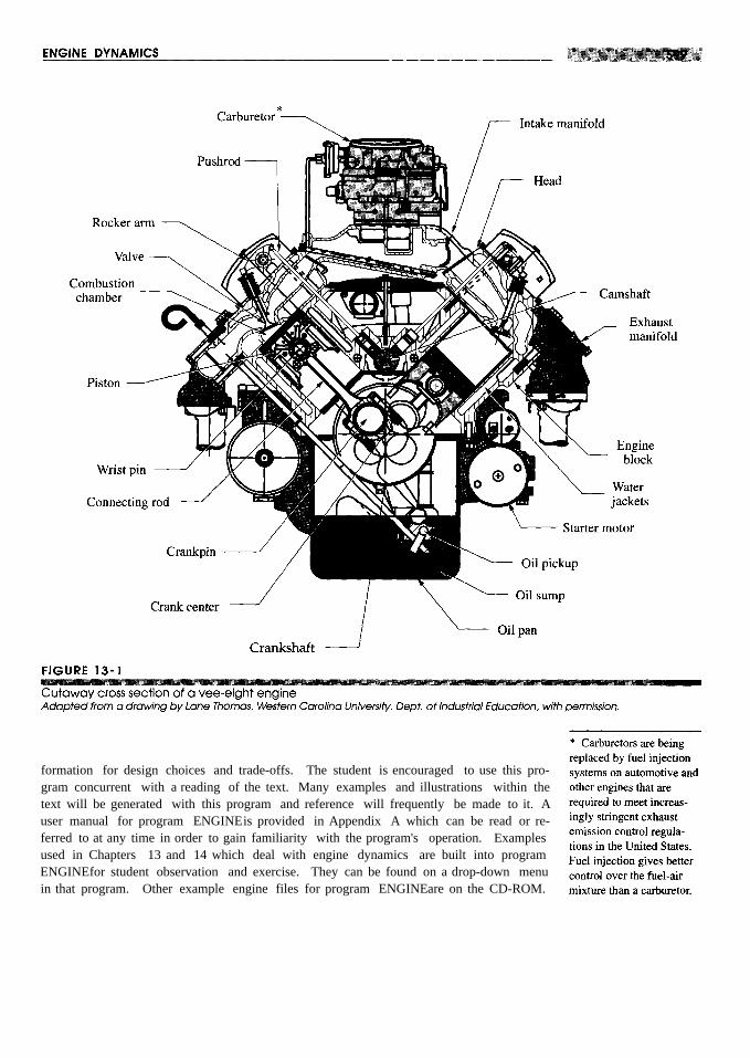
formation for design choices and trade-offs. The student is encouraged to use this pro-gram concurrent with a reading of the text. Many examples and illustrations within thetext will be generated with this program and reference will frequently be made to it. Auser manual for program ENGINEis provided in Appendix A which can be read or re-ferred to at any time in order to gain familiarity with the program's operation. Examplesused in Chapters 13 and 14 which deal with engine dynamics are built into programENGINEfor student observation and exercise. They can be found on a drop-down menuin that program. Other example engine files for program ENGINEare on the CD-ROM.

13.1 ENGINE DESIGN
Figure 13-1 (p. 599) shows a detailed cross section of an internal combustion engine.The basic mechanism consists of a crank, a connecting rod (coupler), and piston (slider).Since this figure depicts a muIticylinder vee-eight engine configuration, there are fourcranks arranged on a crankshaft, and eight sets of connecting rods and pistons, four inthe left bank of cylinders and four in the right bank. Only two piston-connecting rod as-semblies are visible in this view, both on a common crankpin. The others are behindthose shown. Figure 13-2 shows finite-element models of a piston, connecting rod andcrankshaft for a four-cylinder inline engine. The most usual arrangement is an inlineengine with cylinders all in a common plane. Three-, four-, five-, and six-cylinder in-line engines are in production the world over. Vee engines in four-, six-, eight-, ten-,and twelve-cylinder versions are also in production, with vee six and vee eight being themost popular vee configurations. The geometric arrangements of the crankshaft and cyl-inders have a significant effect on the dynamic condition of the engine. We will explorethese effects of multicylinder arrangements in the next chapter. At this stage we wish todeal only with the design of a single-cylinder engine. After optimizing the geometryand dynamic condition of one cylinder, we will be ready to assemble combinations ofcylinders into multicylinder configurations.
A schematic of the basic one-cylinder slider-crank mechanism and the terminolo-gy for its principal parts are shown in Figure 13-3. Note that it is "back-driven" com-

pared to the linkages we have been analyzing in previous chapters. That is, the explo-sion of the combustible mixture in the cylinder drives the piston to the left in Figure 13-3 or down in Figure 13-4, turning the crank. The crank torque that results is ultimatelydelivered to the drive wheels of the vehicle through a transmission (see Section 9.11,p. 474) to propel the car, motorcycle, or other device. The same slider-crank mechanismcan also be used "forward-driven," by motor-driving the crank and taking the outputenergy from the piston end. It is then called a piston pump and is used to compress air,pump gasoline and well water, etc.
In the internal combustion engine of Figure 13-3, it should be fairly obvious that atmost we can only expect energy to be delivered from the exploding gases to the crankduring the power stroke of the cycle. The piston must return from bottom dead center(BDC) to top dead center (TDC) on its own momentum before it can receive anotherpush from the next explosion. In fact, some rotational kinetic energy must be stored inthe crankshaft merely to carry it through the TDC and BDC points as the moment armfor the gas force at those points is zero. This is why an internal combustion engine mustbe "spun-up" with a hand crank, pull rope, or starter motor to get it running.
There are two common combustion cycles in use in internal combustion engines, theClerk two-stroke cycle and the Otto four-stroke cycle, named after their nineteenthcentury inventors. The four-stroke cycle is most common in automobile, truck, and sta-tionary gasoline engines. The two-stroke cycle is used in motorcycles, outboard motors,chain saws, and other applications where its better power-to-weight ratio outweighs itsdrawbacks of higher pollution levels and poor fuel economy compared to the four-stroke.
FOUR-STROKE CYCLE The Otto four-stroke cycle is shown in Figure 13-4. Ittakes four full strokes of the piston to complete one Otto cycle. A piston stroke is de-fined as its travel from TDC to BDC or the reverse. Thus there are two strokes per 3600
crank revolution and it takes 7200 of crankshaft rotation to complete one four-strokecycle. This engine requires at least two valves per cylinder, one for intake and one forexhaust. For discussion, we can start the cycle at any point as it repeats every two crank

revolutions. Figure 13-4a shows the intake stroke which starts with the piston at TDC.A mixture of fuel and air is drawn into the cylinder from the induction system (the fuelinjectors, or the carburetor and intake manifold in Figure 13-1, p. 599) as the piston de-scends to BDC, increasing the volume of the cylinder and creating a slight negative pressure.
During the compression stroke in Figure l3-4b, all valves are closed and the gas iscompressed as the piston travels from BDC to TDC. Slightly before TDC, a spark isignited to explode the compressed gas. The pressure from this explosion builds very

quickly and pushes the piston down from TDC to BDC during the power stroke shownin Figure 13-4c. The exhaust valve is opened and the piston's exhaust stroke from BDCto TDC (Figure 13-4d) pushes the spent gases out of the cylinder into the exhaust man-ifold (see also Figure 13-1) and thence to the catalytic converter for cleaning before be-ing dumped out the tailpipe. The cycle is then ready to repeat with another intake stroke.The valves are opened and closed at the right times in the cycle by a camshaft which isdriven in synchrony with the crankshaft by gears, chain, or toothed belt drive. (See Fig-ure 9-24, p. 452.) Figure 13-4e shows the gas pressure curve for one cycle. With a one-cylinder Otto cycle engine, power is delivered to the crankshaft, at most, 25% of the timeas there is only 1 power stroke per 2 revolutions.
TWO-STROKE CYCLE The Clerk two-stroke cycle is shown in Figure 13-5. Thisengine does not need any valves, though to increase its efficiency it is sometimes pro-vided with a passive (pressure differential operated) one at the intake port. It does nothave a camshaft or valve train or cam drive gears to add weight and bulk to the engine.As its name implies, it requires only two-strokes, or 3600
, to complete its cycle. There isa passageway, called a transfer port, between the combustion chamber above the pistonand the crankcase below. There is also an exhaust port in the side of the cylinder. Thepiston acts to sequentially block or expose these ports as it moves up and down. Thecrankcase is sealed and mounts the carburetor on it, serving also as the intake manifold.
Starting at TDC (Figure 13-5a), the two-stroke cycle proceeds as follows: The sparkplug ignites the fuel-air charge, compressed on the previous revolution. The expansionof the burning gases drives the piston down, delivering torque to the crankshaft. Part-way down, the piston uncovers the exhaust port, allowing the burnt (and also some un-burned) gases to begin to escape to the exhaust system.
As the piston descends (Figure 13-5ba), it compresses the charge of fuel-air mixturein the sealed crankcase. The piston blocks the intake port preventing blowback throughthe carburetor. As the piston clears the transfer port in the cylinder wall, its downwardmotion pushes the new fuel-air charge up through the transfer port to the combustionchamber. The momentum of the exhaust gases leaving the chamber on the other sidehelps pull in the new charge as well.
The piston passes BDC (Figure 13-5c) and starts up, pushing out the remaining ex-haust gases. The exhaust port is closed by the piston as it ascends, allowing compres-sion of the new charge. As the piston approaches TDC, it exposes the intake port (Fig-ure 13-5d), sucking a new charge of air and fuel into the expanded crankcase from thecarburetor. Slightly before TDC, the spark is ignited and the cycle repeats as the pistonpasses TDC.
Clearly, this Clerk cycle is not as efficient as the Otto cycle in which each event ismore cleanly separated from the others. Here there is much mixing of the various phas-es of the cycle. Unburned hydrocarbons are exhausted in larger quantities. This accountsfor the poor fuel economy and dirty emissions of the Clerk engine.* It is neverthelesspopular in applications where low weight is paramount.
Lubrication is also more difficult in the two-stroke engine than in the four-stroke asthe crankcase is not available as an oil sump. Thus the lubricating oil must be mixed withthe fuel. This further increases the emissions problem compared to the Otto cycle enginewhich bums raw gasoline and pumps its lubricating oil separately throughout the engine.


DIESEL CYCLE The diesel cycle can be either two-stroke or four-stroke. It is acompression-ignition cycle. No spark is needed to ignite the air-fuel mixture. The airis compressed in the cylinder by a factor of about 14 to 15 (versus 8 to 10 in the sparkengine), and a low volatility fuel is injected into the cylinder just before TDC. The heatof compression causes the explosion. Diesel engines are larger and heavier than sparkignition engines for the same power output because the higher pressures and forces atwhich they operate require stronger, heavier parts. Two-stroke cycle Diesel engines arequite common. Diesel fuel is a better lubricant than gasoline.
GAS FORCE In all the engines discussed here, the usable output torque is creat-ed from the explosive gas pressure generated within the cylinder either once or twice pertwo revolutions of the crank, depending on the cycle used. The magnitude and shape ofthis explosion pressure curve will vary with the engine design, stroke cycle, fuel used,speed of operation, and other factors related to the thermodynamics of the system. Forour purpose of analyzing the mechanical dynamics of the system, we need to keep thegas pressure function consistent while we vary other design parameters in order to com-pare the results of our mechanical design changes. For this purpose, program ENGINEhas been provided with a built-in gas pressure curve whose peak value is about 600 psiand whose shape is similar to the curve from a real engine. Figure 13-6 shows the gasforce curve that results from the built-in gas pressure function in program ENGINE ap-plied to a piston of particular area, for both two- and four-stroke engines. Changes inpiston area will obviously affect the gas force magnitude for this consistent pressurefunction, but no changes in engine design parameters input to this program will changeits built-in gas pressure curve. To see this gas force curve, run program ENGINE and se-lect anyone of the example engines from the pull-down menu. Then calculate and plotGas Force.
13.2 SLIDER-CRANK KINEMATICS
In Chapters 4, 6, 7, and 11 we developed general equations for the exact solution of thepositions, velocities, accelerations, and forces in the pin-jointed fourbar linkage, and alsofor two inversions of the slider-crank linkage, using vector equations. We could againapply that method to the analysis of the "standard" slider-crank linkage, used in the ma-jority of internal combustion engines, as shown in Figure 13-7. Note that its slider mo-tion has been aligned with the X axis. This is a "nonoffset" slider-crank, because the slid-er axis extended passes through the crank pivot. It also has its slider block translatingagainst the stationary ground plane; thus there will be no Coriolis component of acceler-ation (see Section 7.3, p. 308).
The simple geometry of this particular inversion of the slider-crank mechanism al-lows a very straightforward approach to the exact analysis of its slider's position, veloc-ity, and acceleration, using only plane trigonometry and scalar equations. Because of thismethod's simplicity and to present an alternative solution approach we will analyze thisdevice again.
Let the crank radius be r and the conrod length be I. The angle of the crank is e, andthe angle that the conrod makes with the X axis is <j>. For any constant crank angularvelocity 00, the crank angle e = oot. The instantaneous piston position is x. Two right tri-angles rqs and lqu are constructed. Then from geometry:


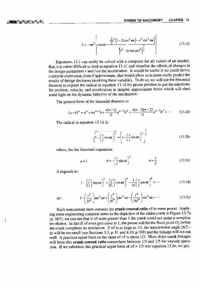

The process of binomial expansion has, in this particular case, led us to Fourier se-ries approximations of the exact expressions for the piston displacement, velocity, andacceleration. Fourier* showed that any periodic function can be approximated by a se-ries of sine and cosine terms of integer multiples of the independent variable. Recall thatwe dropped the fourth, sixth, and subsequent power terms from the binomial expansion,which would have provided cos 400t, cos 600t, etc., terms in this expression. These mul-tiple angle functions are referred to as the harmonics of the fundamental cos rot term.The cos rot term repeats once per crank revolution and is called the fundamental frequen-cy or the primary component. The second harmonic, cos 20)t, repeats twice per crankrevolution and is called the secondary component. The higher harmonics were droppedwhen we truncated the series. The constant term in the displacement function is the DCcomponent or average value. The complete function is the sum of its harmonics. TheFourier series form of the expressions for displacement and its derivatives lets us see therelative contributions of the various harmonic components of the functions. This ap-proach will prove to be quite valuable when we attempt to dynamically balance an en-gine design.
Program ENGINE calculates the position, velocity, and acceleration of the piston ac-cording to equations 13.3c, d, and e. Figure 13-8a, b, and c shows these functions for

The negative sign is due to the choice of engine orientation in the coordinate systemof Figure 13-3. The gas pressure Pg in this expression is a function of crank angle rotand is defined by the thermodynamics of the engine. A typical gas pressure curve fora four-stroke engine is shown in Figure 13-4 (p. 602). The gas force curve shape is iden-tical to that of the gas pressure curve as they differ only by a constant multiplier, the pis-ton areaAp. Figure 13-6 (p. 606) shows the approximation of the gas force curve used inprogram ENGINE for both four- and two-stroke engines.
The gas torque in Figure 13-9 is due to the gas force acting at a moment arm aboutthe crank center 02 in Figure 13-7 (p. 607). This moment arm varies from zero to a max-imum as the crank rotates. The distributed gas force over the piston surface has been re-solved to a single force acting through the mass center of link 4 in the free-body diagramsof Figure 13-7b. The concurrent force system at point B is resolved in the vector dia-gram showing that:


larity in shape to that of the gas force curve in Figure 13-6 (p. 606). Note also that thetwo-stroke has theoretically twice the power available as the four-stroke, all other fac-tors equal, because there are twice as many torque pulses per unit time. The poorer effi-ciency of the two-stroke reduces this theoretical advantage, however.
13.4 EQUIVALENT MASSES
To do a complete dynamic force analysis on any mechanism we need to know the geo-metric properties (mass, center of gravity, mass moment of inertia) of the moving linksas was discussed in previous chapters (see Sections 10.3 to 10.8 and Chapter 11). Thisis easy to do if the link already is designed in detail and its dimensions are known. Whendesigning the mechanism from scratch, we typically do not yet know that level of detailabout the links' geometries. But we must nevertheless make some estimate of their geo-metric parameters in order to begin the iteration process which will eventually convergeon a detailed design.
In the case of this slider-crank mechanism, the crank is in pure rotation and thepiston is in pure translation. By assuming some reasonable geometries and materialswe can make approximations of their dynamic parameters. Their kinematic motions areeasily determined. We have already derived expressions for the piston motion in equa-tions 13.3 (p. 609). Further, if we balance the rotating crank, as described and recom-mended in the previous chapter, then the CG of the crank will be motionless at its center02 and will not contribute to the dynamic forces. We will do this in a later section.
The conrod is in complex motion. To do an exact dynamic analysis as was derivedin Section 11.5, we need to determine the linear acceleration of its CG for all positions.At the outset of the design, the conrod's CG location is not accurately defined. To "boot-strap" the design, we need a simplified model of this connecting rod which we can laterrefine, as more dynamic information is generated about our engine design. The require-ments for a dynamically equivalent model were stated in Section 10.2 and are repeatedhere as Table 13-1 for your convenience.
If we could model our still-to-be-designed conrod as two, lumped, point masses,concentrated one at the crankpin (point A in Figure 13-7, p. 607), and one at the wrist pin(point B in Figure 13-7), we would at least know what the motions of these lumps are.The lump at A would be in pure rotation as part of the crank, and the lump at point Bwould be in pure translation as part of the piston. These lumped, point masses have nodimension and are assumed to be connected with a magical, massless but rigid rod. *
DYNAMICALLY EQUIVALENT MODEL Figure 13-10a shows a typical conrod.Figure 13-10b shows a generic two-mass model of the conrod. One mass mt is locatedat distance It from the CG of the original rod, and the second mass mp at distance lp fromthe CG. The mass of the original part is m3, and its moment of inertia about its CG isIG3. Expressing the three requirements for dynamic equivalence from Table 13-1 math-ematically in terms of these variables, we get:


These define the amounts of the total conrod mass to be placed at each end, to ap-proximately dynamically model that link. Figure 13-lOd shows this dynamic model. Inthe absence of any data on the shape of the conrod at the outset of a design, preliminarydynamic force information can be obtained by using the rule of thumb of placing two-thirds of the conrod's mass at the crankpin and one-third at the wrist pin.
STATICALLY EQUIVALENT MODEL We can create a similar lumped mass modelof the crank. Even though we intend to balance the crank before we are done, for gener-ality we will initially model it unbalanced as shown in Figure 13-11. Its CG is located atsome distance rG2 from the pivot, 02, on the line to the crankpin, A. We would like to
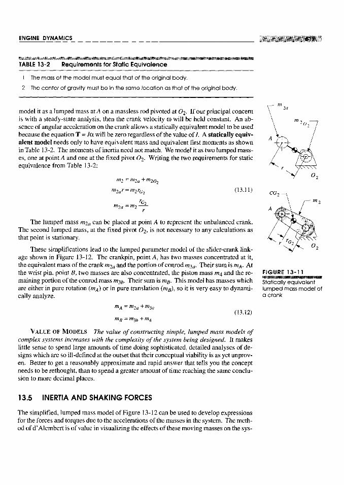


Note that the gas force from equation 13.4 does not contribute to the shaking force.Only inertia forces and external forces are felt as shaking forces. The gas force is aninternal force which is cancelled within the mechanism. It acts equally and oppositelyon both the piston top and the cylinder head as shown in Figure 13-7 (p. 607).
Program ENGINE calculates the shaking force at constant 00, for any combination oflinkage parameters input to it. Figure 13-13 shows the shaking force plot for the sameunbalanced built-in example engine as shown in the acceleration plot (Figure l3-8c,p.611). The linkage orientation is the same as in Figure 13-12 (p. 618) with the x axishorizontal. The x component is larger than the y component due to the high accelerationof the piston. The forces are seen to be quite large despite this being a relatively small(0.4 liter per cylinder) engine running at moderate speed (3400 rpm). We will soon in-vestigate techniques to reduce or eliminate this shaking force from the engine. It is anundesirable feature which creates noise and vibration.
13.6 INERTIA AND SHAKING TORQUES
The inertia torque results from the action of the inertia forces at a moment arm. Theinertia force at point A in Figure 13-12 has two components, radial and tangential. Theradial component has no moment arm. The tangential component has a moment arm ofcrank radius r. If the crank 00 is constant, the mass at A will not contribute to inertiatorque. The inertia force at B has a nonzero component perpendicular to the cylinder wallexcept when the piston is at TDC or BDC. As we did for the gas torque, we can expressthe inertia torque in terms ofthe couple -Fi41, Fi41 whose forces act always perpendic-ular to the motion of the slider (neglecting friction), and the distance x, which is their in-stantaneous moment arm. The inertia torque is:

Program ENGINE calculates the inertia torque from equation B.15e. Figure 13-14shows a plot of the inertia torque for this built-in example engine. Note the dominanceof the second harmonic. The ideal magnitude for the inertia torque is zero, as it is para-sitic. Its average value is always zero, so it contributes nothing to the net driving torque.It merely creates large positive and negative oscillations in the total torque which in-crease vibration and roughness. We will soon investigate means to reduce or eliminatethis inertia and shaking torque in our engine designs. It is possible to cancel their ef-fects by proper arrangement of the cylinders in a multicylinder engine, as will be ex-plored in the next chapter.

13.8 FLYWHEELS
We saw in Section 11.11 (p. 548) that large oscillations in the torque-time function canbe significantly reduced by the addition of a flywheel to the system. The single-cylinderengine is a prime candidate for the use of a flywheel. The intermittent nature of its pow-er strokes makes one mandatory as it will store the kinetic energy needed to carry thepiston through the Otto cycle's exhaust, intake, and compression strokes during whichwork must be done on the system. Even the two-stroke engine needs a flywheel to drivethe piston up on the compression stroke.
The procedure for designing an engine flywheel is identical to that described in Sec-tion 11.11 for the fourbar linkage. The total torque function for one revolution of thecrank is integrated, pulse by pulse, with respect to its average value. These integrals rep-resent energy fluctuations in the system. The maximum change in energy under thetorque curve during one cycle is the amount needed to be stored in the flywheel. Equa-

tion 11.20c expresses this relationship. Program ENGINE does the numerical integrationof the total torque function and presents a table similar to the one shown in Figure 11-11(p. 551). These data and the designer's choice of a coefficient of fluctuation k (see equa-tion 11.19) are all that are needed to solve equations 11.20 and 11.21 for the requiredmoment of inertia of the flywheel.
The calculation must be done at some average crank 0). Since the typical engine op-erates over a wide range of speeds, some thought needs to be given to the most appropri-ate speed to use in the flywheel calculation. The flywheel's stored kinetic energy is pro-portional to co2 (see equation 11.17). Thus at high speeds a flywheel can have a smallmoment of inertia and still be effective. The slowest operating speed will require thelargest flywheel and should be the one used in the computation of required flywheel size.
Program ENGINE plots the flywheel-smoothed total torque for a user-supplied coef-ficient of fluctuation k. Figure 13-16 shows the smoothed torque functions for k = 0.05corresponding to the un smoothed ones in Figure 13-15. Note that the smoothed curvesshown for each engine speed are what would result with the flywheel size necessary toobtain that coefficient of fluctuation at that speed. In other words, the flywheel appliedto the 800-rpm engine is much larger than the one on the 6000-rpm engine, in these plots.Compare corresponding rows (speeds) between Figures 13-15 and 13-16 to see the ef-fect of the addition of a flywheel. But do not directly compare parts a, b, and c withinFigure 13-16 as to the amount of smoothing since the flywheel sizes used are different ateach operating speed.
An engine flywheel is usually designed as a flat disk, bolted to one end of the crank-shaft. One flywheel face is typically used for the clutch to run against. The clutch is afriction device which allows disconnection of the engine from the drive train (the wheelsof a vehicle) when no output is desired. The engine can then remain running at idle speedwith the vehicle or output device stopped. When the clutch is engaged, all engine torqueis transmitted through it, by friction, to the output shaft.
13.9 PIN FORCES IN THESINGLE-CYLINDER ENGINE
In addition to calculating the overall effects on the ground plane of the dynamic forcespresent in the engine, we also need to know the magnitudes of the forces at the pin joints.These forces will dictate the design of the pins and the bearings at the joints. Though wewere able to lump the mass due to both conrod and piston, or conrod and crank, at pointsA and B for an overall analysis of the linkage's effects on the ground plane, we cannot doso for the pin force calculations. This is because the pins feel the effect of the conrodpulling on one "side" and the piston (or crank) pulling on the other "side" of the pin asshown in Figure 13-17. Thus we must separate the effects of the masses of the linksjoined by the pins.
We will calculate the effect of each component due to the various masses, and thegas force and then superpose them to obtain the complete pin force at each joint. Weneed a bookkeeping system to keep track of all these components. We have already usedsome subscripts for these forces, so we will retain them and add others. The resultantbearing loads have the following components:


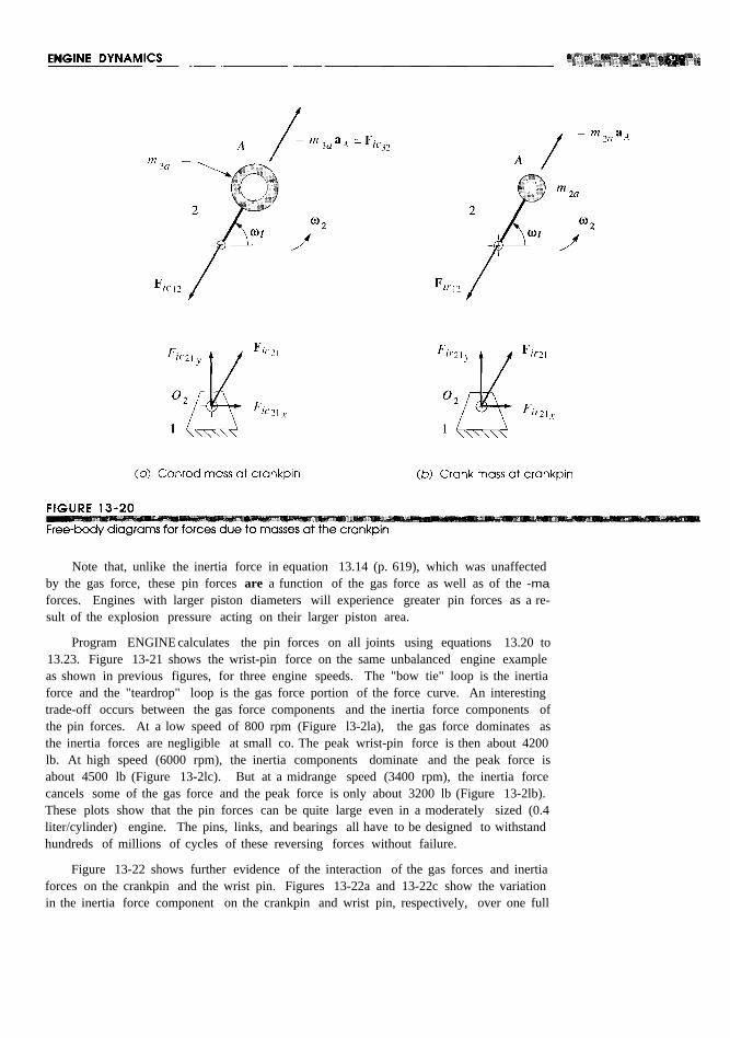
Note that, unlike the inertia force in equation 13.14 (p. 619), which was unaffectedby the gas force, these pin forces are a function of the gas force as well as of the -maforces. Engines with larger piston diameters will experience greater pin forces as a re-sult of the explosion pressure acting on their larger piston area.
Program ENGINE calculates the pin forces on all joints using equations 13.20 to13.23. Figure 13-21 shows the wrist-pin force on the same unbalanced engine exampleas shown in previous figures, for three engine speeds. The "bow tie" loop is the inertiaforce and the "teardrop" loop is the gas force portion of the force curve. An interestingtrade-off occurs between the gas force components and the inertia force components ofthe pin forces. At a low speed of 800 rpm (Figure l3-2la), the gas force dominates asthe inertia forces are negligible at small co. The peak wrist-pin force is then about 4200lb. At high speed (6000 rpm), the inertia components dominate and the peak force isabout 4500 lb (Figure 13-2lc). But at a midrange speed (3400 rpm), the inertia forcecancels some of the gas force and the peak force is only about 3200 lb (Figure 13-2lb).These plots show that the pin forces can be quite large even in a moderately sized (0.4liter/cylinder) engine. The pins, links, and bearings all have to be designed to withstandhundreds of millions of cycles of these reversing forces without failure.
Figure 13-22 shows further evidence of the interaction of the gas forces and inertiaforces on the crankpin and the wrist pin. Figures 13-22a and 13-22c show the variationin the inertia force component on the crankpin and wrist pin, respectively, over one full


revolution of the crank as the engine speed is increased from idle to redline. Figure13-22b and d show the variation in the total force on the same respective pins with boththe inertia and gas force components included. These two plots show only the first 900
of crank revolution where the gas force in a four-stroke cylinder occurs. Note that thegas force and inertia force components counteract one another resulting in one particu-lar speed where the total pin force is a minimum during the power stroke. This is thesame phenomenon as seen in Figure 13-21.
13.10 BALANCING THESINGLE-CYLINDER ENGINE
The derivations and figures in the preceding sections have shown that significant forcesare developed both on the pivot pins and on the ground plane due to the gas forces andthe inertia and shaking forces. Balancing will not have any effect on the gas forces,which are internal, but it can have a dramatic effect on the inertia and shaking forces.The main pin force can be reduced, but the crankpin and wrist pin forces will be unaf-fected by any crankshaft balancing done. Figure 13-13 (p. 620) shows the unbalancedshaking force as felt on the ground plane of our OA-liter-per-cylinder example enginefrom program ENGINE. It is about 9700 Ib even at the moderate speed of 3400 rpm. At6000 rpm it increases to over 30 000 lb. The methods of Chapter 12 can be applied to thismechanism to balance the members in pure rotation and reduce these large shaking forces.
Figure 13-23a shows the dynamic model of our slider-crank with the conrod masslumped at both crankpin A and wrist pin B. We can consider this single-cylinder engineto be a single-plane device, thus suitable for static balancing (see Section 13.1). It isstraightforward to statically balance the crank. We need a balance mass at some radius,1800 from the lumped mass at point A whose mr product is equal to the product of themass at A and its radius r. Applying equation 13.2 to this simple problem we get:
Any combination of mass and radius which gives this product, placed at 1800 frompoint A will balance the crank. For simplicity of example, we will use a balance radiusequal to r. Then a mass equal to mA placed at A ' will exactly balance the rotating mass-es. The CG ofthe crank will then be at the fixed pivot 02 as shown in Figure 13-23a. Ina real crankshaft, actually placing the counterweight at this large a radius would notwork. The balance mass has to be kept close to the centerline to clear the piston at BDC.Figure 13-2c shows the shape of typical crankshaft counterweights.
Figure 13-24a shows the shaking force from the same engine as in Figure 13-13 af-ter the crank has been exactly balanced in this manner. The Y component of the shakingforce has been reduced to zero and the x component to about 3300 Ib at 3400 rpm. Thisis a factor of three reduction over the unbalanced engine. Note that the only source of Ydirected inertia force is the rotating mass at point A of Figure 13-23 (see equations 13.14,p. 619). What remains after balancing the rotating mass is the force due to the accelera-tion of the piston and conrod masses at point B of Figure 13-23 which are in linear trans-lation along the X axis, as shown by the inertia force -mBaB at point B in that figure.
To completely eliminate this reciprocating unbalanced shaking force would requirethe introduction of another reciprocating mass, which oscillates 1800 out of phase withthe piston. Adding a second piston and cylinder, properly arranged, can accomplish this.


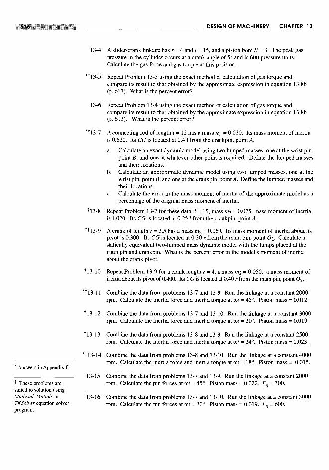


14.0 INTRODUCTION
The previous chapter discussed the design of the slider-crank mechanism as used in thesingle-cylinder internal combustion engine and piston pumps. We will now extend thedesign to multicylinder configurations. Some of the problems with shaking forces andtorques can be alleviated by proper combination of multiple slider-crank linkages on acommon crankshaft. Program ENGINE, included with this text, will calculate the equa-tions derived in this chapter and allow the student to exercise many variations of an en-gine design in a short time. Some examples are provided as disk files to be read into theprogram. These are noted in the text. The student is encouraged to investigate these ex-amples with program ENGINE in order to develop an understanding of and insight to thesubtleties of this topic. A user manual for program ENGINE is provided in Appendix Awhich can be read or referred to out of sequence, with no loss in continuity, in order togain familiarity with the program's operation.
As with the single-cylinder case, we will not address the thermodynamic aspects ofthe internal combustion engine beyond the definition of the combustion forces necessaryto drive the device presented in the previous chapter. We will concentrate on the engine'skinematic and mechanical dynamics aspects. It is not our intention to make an "enginedesigner" of the student so much as to apply dynamic principles to a realistic designproblem of general interest and also to convey the complexity and fascination involvedin the design of a more complicated dynamic device than the single-cylinder engine.
639


14.1 MUlTICYLINDER ENGINE DESIGNS
Multicylinder engines are designed in a wide variety of configurations from the simpleinline arrangement to vee, opposed, and radial arrangements some of which are shownin Figure 14-1. These arrangements may use any of the stroke cycles discussed in Chap-ter 13, Clerk, Otto, or Diesel.
IN LINE ENGINES The most common and simplest arrangement is an inline enginewith its cylinders all in a common plane as shown in Figure 14-2. Two-,* three-,* four,five, and six-cylinder inUne engines are in common use. Each cylinder will have its in-dividual slider-crank mechanism consisting of a crank, conrad, and piston. The cranksare formed together in a common crankshaft as shown in Figure 14-3. Each cylinder'scrank on the crankshaft is referred to as a crank throw. These crank throws will be ar-ranged with some phase angle relationship one to the other, in order to stagger the mo-tions of the pistons in time. It should be apparent from the discussion of shaking forcesand balancing in the previous chapter that we would like to have pistons moving in op-posite directions to one another at the same time in order to cancel the reciprocating in-ertial forces. The optimum phase angle relationships between the crank throws will dif-fer depending on the number of cylinders and the stroke cycle of the engine. There willusually be one (or a small number at) viable crank throw arrangements for a given en-gine configuration to accomplish this goal. The engine in Figure 14-2 is a four-strokecycle, four-cylinder, inline engine with its crank throws at 0, 180, 180, and 0° phaseangles which we will soon see are optimum for this engine. Figure 14-3 shows the crank-shaft, connecting rods and pistons for the same design of engine as in Figure 14-2.


VEE ENGINES in two-, * four-, * six-, eight-, ten-, t and twelve-cylinder+ versionsare produced, with vee six and vee eight being the most common configurations. Figure14-4 shows a cross section and Figure 14-5 a cutaway of a 60° vee -twelve engine. Veeengines can be thought of as two inline engines grafted together onto a common crank-shaft. The two "inline" portions, or banks, are arranged with some vee angle betweenthem. Figure 14-ld shows a vee-eight engine. Its crank throws are at 0,90,270, and180° respectively. A vee eight's vee angle is 90°. The geometric arrangements of thecrankshaft (phase angles) and cylinders (vee angle) have a significant effect on the dy-namic condition of the engine. We will soon explore these relationships in detail.
OPPOSED ENGINES are essentially vee engines with a vee angle of 180°. The pis-tons in each bank are on opposite sides of the crankshaft as shown in Figure 14-6. Thisarrangement promotes cancellation of inertial forces and is popular in aircraft engines. §It has also been used in some automotive applications. II
RADIAL ENGINES have their cylinders arranged radially around the crankshaft innearly a common plane. These were common on World War II vintage aircraft as theyallowed large displacements, and thus high power, in a compact form whose shape waswell suited to that of an airplane. Typically air cooled, the cylinder arrangement allowedgood exposure of all cylinders to the airstream. Large versions had multiple rows of ra-dial cylinders, rotationally staggered to allow cooling air to reach the back rows. Thegas turbine jet engine has rendered these radial aircraft engines obsolete.
ROTARY ENGINES were an interesting variant on the aircraft radial engine. Sim-ilar in appearance and cylinder arrangement to the radial engine, the anomaly was thatthe crankshaft was the stationary ground plane. The propeller was attached to the crank-case (block) which rotated around the crankshaft! It is a kinematic inversion of the radi-al engine. At least it didn't need a flywheel.
Many other configurations of engines have been tried over the century of develop-ment of this ubiquitous device. The bibliography at the end of this chapter contains sev-eral references which describe other engine designs, the usual, unusual, and exotic. Wewill begin our detailed exploration of multicylinder engine design with the simplest con-figuration, the inline engine, and then progress to the vee and opposed versions.

We must establish some convention for the measurement of these phase angleswhich will be:
1 The first (front) cylinder will be number 1 and its phase angle will always be zero.It is the reference cylinder for all others.
2 The phase angles of all other cylinders will be measured with respect to the crankthrow for cylinder 1.
3 Phase angles are measured internal to the crankshaft, that is, with respect to a rotat-ing coordinate system embedded in the first crank throw.
4 Cylinders will be numbered consecutively from front to back of the engine.
The phase angles are defined in a crank phase diagram as shown in Figure 14-7for a four-cylinder, inline engine. Figure l4-7a shows the crankshaft with the throwsnumbered clockwise around the axis. The shaft is rotating counterclockwise. The pis-tons are oscillating horizontally in this diagram, along the x axis. Cylinder 1 is shownwith its piston at top dead center (TDC). Taking that position as the starting point for theabscissas (thus time zero) in Figure 14-7b, we plot the velocity of each piston for tworevolutions of the crank (to accommodate one complete four-stroke cycle). Piston 2 ar-rives at TDC 90° after piston 1 has left. Thus we say that cylinder 2 lags cylinder 1 by90 degrees. By convention a lagging event is defined as having a negative phase angle,shown by the clockwise numbering of the crank throws. The velocity plots clearly showthat each cylinder arrives at TDC (zero velocity) 90° later than the one before it. Nega-tive velocity on the plots in Figure l4-7b indicates piston motion to the left (down stroke)in Figure l4-7a; positive velocity indicates motion to the right (up stroke).
For the discussion in this chapter we will assume counterclockwise rotation of allcrankshafts, and all phase angles will thus be negative. We will, however, omit the neg-ative signs on the listings of phase angles with the understanding that they follow thisconvention.
Figure 14-7 shows the timing of events in the cycle and is a necessary and usefulaid in defining our crankshaft design. However, it is not necessary to go to the trouble ofdrawing the correct sinusoidal shapes of the velocity plots to obtain the needed informa-tion. All that is needed is a schematic indication of the relative positions within the cy-

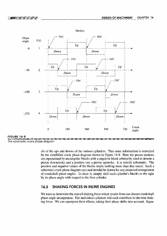


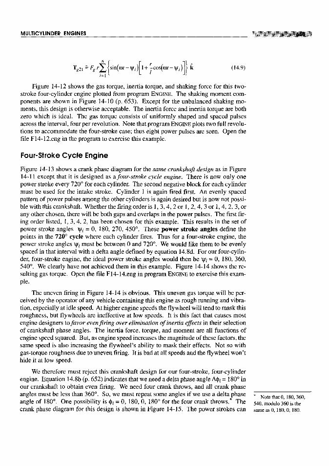


14.8b, p. 652) should reveal that, in this example, each four-cylinder bank has potential-ly 720/4 = 180° between power pulses. Our chosen crank throws are spaced at 90° in-crements. A 90° bank angle will be optimum in this case as the phase angles and bankangles will add to create an effective spacing of 180°. Every vee engine design will haveone or more optimum vee angles that will give approximately even firing with any par-ticular set of crank phase angles.
Several firing orders are possible with this many cylinders. Vee engines are oftenarranged to fire cylinders in opposite banks successively to balance the fluid flow de-mands in the intake manifold. Our cylinders are numbered from front to back, first downthe right bank and then down the left bank. The firing order shown in Figure 14-23b is


Unbalanced shaking forces and shaking moments can be cancelled by the additionof one or more rotating balance shafts within the engine. To cancel the primary compo-nents requires two balance shafts rotating at crank speed, one of which can be the crank-shaft itself. To cancel the secondary components usually requires at least two balanceshafts rotating at twice crank speed, gear or chain driven from the crankshaft. Figure14-26a shows a pair of counterrotating shafts which are fitted with eccentric masses ar-ranged 1800 out of phase. * As shown, the unbalanced centrifugal forces from the equal,unbalanced masses will add to give a shaking force component in the vertical directionof twice the unbalanced force from each mass, while their horizontal components willexactly cancel. Pairs of counterrotating eccentrics can be arranged to provide a harmon-ically varying force in anyone plane. The harmonic frequency will be determined bythe rotational speed of the shafts.
If we arrange two pairs of eccentrics, with one pair displaced some distance alongthe shaft from the other, and also rotated 1800 around the shaft from the first, as shown

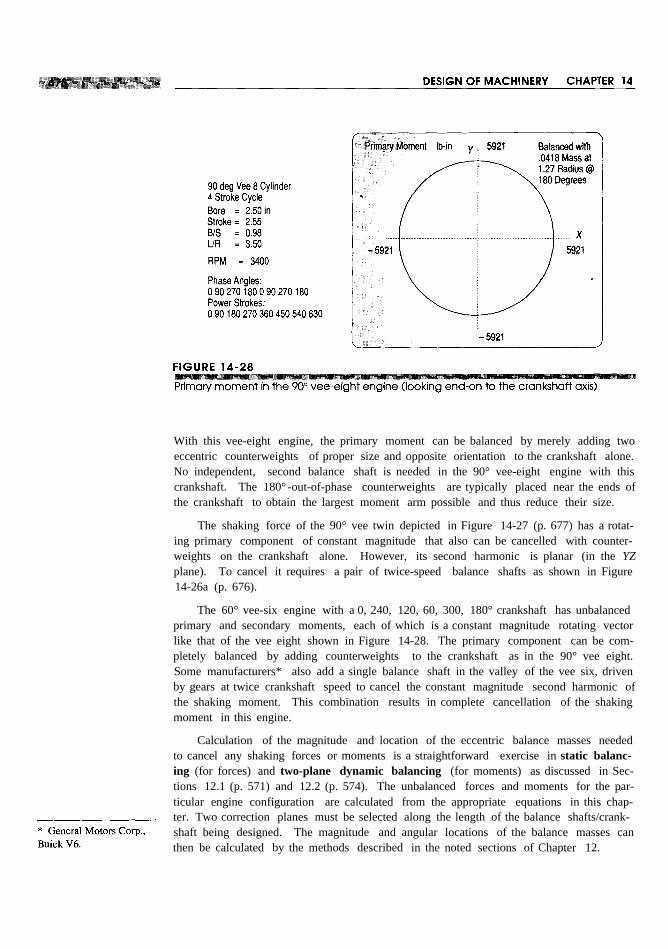
With this vee-eight engine, the primary moment can be balanced by merely adding twoeccentric counterweights of proper size and opposite orientation to the crankshaft alone.No independent, second balance shaft is needed in the 90° vee-eight engine with thiscrankshaft. The 180° -out-of-phase counterweights are typically placed near the ends ofthe crankshaft to obtain the largest moment arm possible and thus reduce their size.
The shaking force of the 90° vee twin depicted in Figure 14-27 (p. 677) has a rotat-ing primary component of constant magnitude that also can be cancelled with counter-weights on the crankshaft alone. However, its second harmonic is planar (in the YZplane). To cancel it requires a pair of twice-speed balance shafts as shown in Figure14-26a (p. 676).
The 60° vee-six engine with a 0, 240, 120, 60, 300, 180° crankshaft has unbalancedprimary and secondary moments, each of which is a constant magnitude rotating vectorlike that of the vee eight shown in Figure 14-28. The primary component can be com-pletely balanced by adding counterweights to the crankshaft as in the 90° vee eight.Some manufacturers* also add a single balance shaft in the valley of the vee six, drivenby gears at twice crankshaft speed to cancel the constant magnitude second harmonic ofthe shaking moment. This combination results in complete cancellation of the shakingmoment in this engine.
Calculation of the magnitude and location of the eccentric balance masses neededto cancel any shaking forces or moments is a straightforward exercise in static balanc-ing (for forces) and two-plane dynamic balancing (for moments) as discussed in Sec-tions 12.1 (p. 571) and 12.2 (p. 574). The unbalanced forces and moments for the par-ticular engine configuration are calculated from the appropriate equations in this chap-ter. Two correction planes must be selected along the length of the balance shafts/crank-shaft being designed. The magnitude and angular locations of the balance masses canthen be calculated by the methods described in the noted sections of Chapter 12.


These are loosely structured design problems intended for solution using program EN-GINE. All involve the design of one or more multicylinder engines and differ mainly inthe specific data for the engine. The general problem statement is:Design a multicylinder engine for a specified displacement and stroke cycle. Optimize the con-rad/crank ratio and bore/stroke ratio to minimize shaking forces, shaking torque, and pin forces,also considering package size. Design your link shapes and calculate realistic dynamic parame-ters (mass, CG location, moment of inertia) for those links using the methods shown in Chapters10 through 13. Dynamically model the links as described in those chapters. Balance or overbal-ance the linkage as needed to achieve the desired results. Choose crankshaft phase angles tooptimize the inertial balance of the engine. Choose afiring order and determine the power strokeangles to optimize even firing. Trade off inertia balance if necessary to achieve even firing.Choose an optimum vee angle if appropriate to the particular problem. Overall smoothness oftotal torque is desired. Design and size a minimum weight flywheel by the method of Chapter 11to smooth the total torque. Write an engineering report on your design and analysis.
PI4-I Two-stroke cycle inline twin with a displacement of I liter.
P14-2 Four-stroke cycle inline twin with a displacement of I liter.
P14-3 Two-stroke cycle vee twin with a displacement of I liter.
P14-4 Four-stroke cycle vee twin with a displacement of I liter.
P14-5 Two-stroke cycle opposed twin with a displacement of I liter.
P14-6 Four-stroke cycle opposed twin with a displacement of I liter.
P14-7 Two-stroke cycle vee four with a displacement of 2 liters.
P14-8 Four-stroke cycle vee four with a displacement of 2 liters.
P14-9 Two-stroke cycle opposed four with a displacement of 2 liters.
P14-10 Four-stroke cycle opposed four with a displacement of 2 liters.
PI4-II Two-stroke inline five cylinder with a displacement of 2.5 liters.
P14-12 Four-stroke inline five cylinder with a displacement of 2.5 liters.

P14-13 Two-stroke cycle vee six with a displacement of 3 liters.
P14-14 Four-stroke cycle vee six with a displacement of 3 liters.
P14-15 Two-stroke cycle opposed six with a displacement of 3 liters.
P14-16 Four-stroke cycle opposed six with a displacement of 3 liters.
P14-17 Two-stroke inline seven cylinder with a displacement of 3.5 liters.
P14-18 Four-stroke inline seven cylinder with a displacement of 3.5 liters.
P14-19 Two-stroke inline eight cylinder with a displacement of 4 liters.
P14-20 Four-stroke inline eight cylinder with a displacement of 4 liters.
P14-21 Two-stroke vee ten cylinder with a displacement of 5 liters.
P14-22 Four-stroke vee ten cylinder with a displacement of 5 liters.
P14-23 Four-stroke W-6 with a displacement of 5 liters. (A W engine has three banks ofcylinders on a common crank.)
P14-24 Four-stroke W-9 with a displacement of 5 liters. (A W engine has three banks ofcylinders on a common crank.)
P14-25 Four-stroke W-12 with a displacement of 5 liters. (A W engine has three banks ofcylinders on a common crank.)
P14-26 Design a family of vee engines to be built on the same assembly line. They must allhave the same vee angle and use the same pistons, connecting rods, and strokes.Their crankshafts can each be different. Four configurations are needed: vee four,vee six, vee eight, and vee ten. All will have the same single-cylinder displacementof 0.5 liters. Optimize the single-cylinder configuration from which the multicylinderengines will be constructed for bore/stroke ratio and conrod crank ratio. Thenassemble this cylinder design into the above configurations. Find the best compro-mise of vee angle to provide a good mix of balance and even firing in all engines.
P14-27 Repeat Project P14-26 for a family ofW engines: W-3, W-6, W-9, and W-12. Theinter-bank angles must be the same for all models. See the built-in example W-12engine in program ENGINEfor more information on this unusual W configuration.
P14-28 In recent years some automobile manufacturers have made unusual vee configura-tions such as the VW-Audi VR15 which is a 15° vee six. Obtain detailed informationon this engine design and then analyze it with program ENGINE. Write a report thatexplains why the manufacturer chose this unusual arrangement and justify yourconclusions with sound engineering analysis.
P14-29 Design an inline six- and an inline five-cylinder engine of the same displacement, say2.5 liters. Analyze their dynamics with program ENGINE. Write an engineeringreport to explain why such manufacturers as Audi, Volvo, and Acura have chosen afive-cylinder inline over a six cylinder of comparable torque and power output.
P14-30 Ferrari has produced vee-twelve engines in both 60° vee and horizontally opposedconfigurations. Design 3-liter versions of each and compare their dynamics. Write areport that explains why the manufacturer chose these arrangements and justify yourconclusions with sound engineering analysis.
P14-31 Design and compare a 3-liter 90° vee six, 60° vee six, inline six, and 180° opposedsix, all of which designs are in volume production. Explain their advantages anddisadvantages and justify your conclusions with sound engineering analysis.

15.0 INTRODUCTION.
Chapter 8 presented the kinematics of cams and followers and methods for their design.We will now extend the study of cam-follower systems to include considerations of thedynamic forces and torques developed. While the discussion in this chapter is limited toexamples of cams and followers, the principles and approaches presented are applicableto most dynamic systems. The cam-follower system can be considered a useful and con-venient example for the presentation of topics such as creating lumped parameter dynam-ic models and defining equivalent systems as described in Chapter 10. These techniquesas well as the discussion of natural frequencies, effects of damping, and analogies be-tween physical systems will be found useful in the analysis of all dynamic systems re-gardless of type.
In Chapter 10 we discussed the two approaches to dynamic analysis, commonlycalled the forward and the inverse dynamics problems. The forward problem assumesthat all the forces acting on the system are known and seeks to solve for the resulting dis-placements, velocities, and accelerations. The inverse problem is, as its name says, theinverse of the other. The displacements, velocities, and accelerations are known, and wesolve for the dynamic forces that result. In this chapter we will explore the applicationof both methods to cam-followerdynamics. Section 15.1 explores the forward solution.Section 15.3 will present the inverse solution. Both are instructive in this application ofa force-closed (spring-loaded) cam-follower system and will each be discussed in thischapter.

15.1 DYNAMIC FORCE ANALYSIS OF THEFORCE-CLOSED CAM-FOLLOWER
Figure l5-la shows a simple plate or disk cam driving a spring-loaded, roller follower.This is a force-closed system which depends on the spring force to keep the cam andfollower in contact at all times. Figure 15-1b shows a lumped parameter model of thissystem in which all the mass which moves with the follower train is lumped together asm, all the springiness in the system is lumped within the spring constant k, and all thedamping or resistance to movement is lumped together as a damper with coefficient c.The sources of mass which contribute to m are fairly obvious. The mass of the followerstem, the roller, its pivot pin, and any other hardware attached to the moving assembly alladd together to create m. Figure l5-lc shows the free-body diagram of the system actedupon by the cam force Fe, the spring force Fs, and the damping force Fd. There will ofcourse also be the effects of mass times acceleration on the system.
Undamped Response
Figure 15-2 shows an even simpler lumped parameter model of the same system as inFigure 15-1 but which omits the damping altogether. This is referred to as a conserva-tive model since it conserves energy with no losses. This is not a realistic or safe assump-tion in this case but will serve a purpose in the path to a better model which will includethe damping. The free-body diagram for this mass-spring model is shown in Figurel5-2c. We can write Newton's equation for this one-DOF system:


15.2 RESONANCE
The natural frequency (and its overtones) are of great interest to the designer as they de-fine the frequencies at which the system will resonate. The single-DOF lumped param-eter systems shown in Figures 15-1 and 15-2 (p. 687) are the simplest possible to describea dynamic system, yet they contain all the basic dynamic elements. Masses and springsare energy storage elements. A mass stores kinetic energy, and a spring stores potentialenergy. The damper is a dissipative element. It uses energy and converts it to heat. Thusall the losses in the model of Figure 15-1 occur through the damper.
These are "pure" idealized elements which possess only their own characteristics.That is, the spring has no damping and the damper no springiness, etc. Any system whichcontains more than one energy storage device such as a mass and a spring will possess atleast one natural frequency. If we excite the system at its natural frequency, we will setup the condition called resonance in which the energy stored in the system's elementswill oscillate from one element to the other at that frequency. The result can be violentoscillations in the displacements of the movable elements in the system as the energymoves from potential to kinetic form and vice versa.
Figure 15-6 shows a plot of the amplitude and phase angle of the displacement re-sponse X of the system to a sinusoidal input forcing function at various frequencies oot-In our case, the forcing frequency is the angular velocity at which the cam is rotating.The plot normalizes the forcing frequency as the frequency ratio oof/ oon. The responseamplitude X is normalized by dividing the dynamic deflection x by the static deflectionF 0/ k that the same force amplitude would create on the system. Thus at a frequency ofzero, the output is one, equal to the static deflection of the spring at the amplitude of theinput force. As the forcing frequency increases toward the natural frequency oon, theamplitude of the output motion, for zero damping, increases rapidly and becomes theo-retically infinite when oof = oon. Beyond this point the amplitude decreases rapidly andasymptotically toward zero at high frequency ratios. It is obvious that we must avoiddriving this system at or near its natural frequency. The addition of damping reduces theamplitude of vibration at the natural frequency, but very large damping ratios (> 0.6) areneeded to keep the output amplitude less than or equal to the input amplitude. This ismuch more damping than is found in cam-follower systems and most machinery. Oneresult of operation of an underdamped cam-follower system near oon can be followerjump. The system of follower mass and spring can oscillate violently at its natural fre-quency and leave contact with the cam. When it does reestablish contact, it may do sowith severe impact loads that can quickly fail the materials.
The designer has a degree of control over resonance in that the system's mass m andstiffness k can be tailored to move its natural frequency away from any required operat-ing frequencies. A common rule of thumb is to design the system to have a fundamentalnatural frequency oon at least ten times the highest forcing frequency expected in service,thus keeping all operation well below the resonance point. This is often difficult toachieve in mechanical systems. One tries to achieve the largest ratio oon / oof possiblenevertheless, even if it is less than 10.
For cams with finite jerk having a dwell after the rise of the same order of durationas the rise, Koster[l] defines a dimensionless ratio,


Thus, the response of a earn-follower system of this type will be dominated by therecurring transient responses rather than by the forced, or steady-state, response. It isimportant to adhere to the fundamental law of earn design and use earn programs withfinite jerk in order to minimize these residual vibrations in the follower system. Koster[1]reports that the cycloidal and 3-4-5 polynomial programs both gave low residual vibra-tions in the double-dwell earn. The modified sine acceleration program will also givegood results. All these have finite jerk. (See Section 8.8 and Table 8-4, p. 421.)
Some thought and observation of equation 15.1d (p. 688) will show that we wouldlike our system members to be both light (low m) and stiff (high k) to get high values for(On and thus low values for 'to Unfortunately, the lightest materials are seldom also thestiffest. Aluminum is one-third the weight of steel but is also about a third as stiff. Tita-nium is about half the weight of steel but also about half as stiff. Some of the exoticcomposite materials such as carbon fiber/epoxy offer better stiffness-to-weight ratios buttheir cost is high and processing is difficult. Another job for Unobtainium 208!
Note in Figure 15-6 (p. 697) that the amplitude of vibration at large frequency ratiosapproaches zero. So, if the system can be brought up to speed through the resonancepoint without damage and then kept operating at a large frequency ratio, the vibrationwill be minimal. An example of systems designed to be run this way are large devicesthat must run at higher speed such as electrical power generators. Their large mass cre-ates a lower natural frequency than their required operating speeds. They are "run up"as quickly as possible through the resonance region to avoid damage from their vibra-tions and "rundown" quickly through resonance when stopping them. They also havethe advantage of long duty cycles of constant speed operation in the safe frequency re-gion between infrequent starts and stops.
15.3 KINETOSTATIC FORCE ANALYSIS OF THEFORCE-CLOSEDCAM-FOLLOWER
The analysis in the previous sections is of the "forward dynamic analysis" type as de-fined in Section 10.1, p. 491. That is, the applied force [F e(t) in equation 15.2b, p. 689]is presumed to be known, and the equation is solved for the resulting displacement x fromwhich its derivatives can also be determined. Carn-follower force analysis problems, likelinkage analysis problems, lend themselves well to solution by the inverse dynamics, orkinetostatics, approach. Here the displacement and its derivatives are defined from thekinematic design of the earn based on an assumed angular velocity (0 of the earn, and wewant to solve for the force Fe(t). Equation 15.2b can be solved directly for the force in aspring-loaded earn-follower system provided that values for mass m, spring constant k,preload Fpz, and darnping factor c are known in addition to the displacement, velocity,and acceleration functions.
The designer has a large degree of control over the system spring constant keff as ittends to be dominated by the ks of the physical return spring. The elasticities of the fol-lower parts also contribute to the overall system keff but are usually much stiffer than thephysical spring. If the follower stiffness is in series with the return spring, as it often is,equation 10.17c (p. 506) shows that the softest spring in series will dominate the effec-tive spring constant. Thus the return spring will virtually determine the overall k unlesssome parts of the follower train have similarly low stiffness.


Given: A translating roller follower as shown in Figure 15-1 is driven by a force-closedradial plate cam which has the following program:
Segment I: Rise I inch in 50° with modified sine accelerationSegment 2: Dwell for 40°Segment 3: Fall I inch in 50° with cycloidal displacementSegment 4: Dwell for 40°Segment 5: Rise I inch in 50° with 3-4-5 polynomial displacementSegment 6: Dwell for 40°Segment 7; Fall I inch in 50° with 4-5-6-7 polynomial displacementSegment 8: Dwell for 40°Camshaft angular velocity is 18.85 rad/sec.Follower effective mass is 0.0738 in-lb-sec2 (blobs).Damping is 15% of critical (s = 0.15).
Problem: Compute the necessary spring constant and spring preload to maintain contact be-tween cam and follower and calculate the dynamic force function for the cam.Calculate the system natural frequency with the selected spring. Keep the pres-sure angle under 30°.
Solution:
I Calculate the kinematic data (follower displacement, velocity, acceleration, and jerk) for thespecified cam functions. The acceleration for this cam is shown in Figure 15-7 and has amaximum value of 3504 inlsec2• See Chapter 8 to review this procedure.
2 Calculate the pressure angle and radius of curvature for trial values of prime circle radius,and size the cam to control these values. Figure 15-8 shows the pressure angle function andFigure 15-9 the radii of curvature for this cam with a prime circle radius of 4 in and zero ec-centricity. The maximum pressure angle is 29.2° and the minimum radius of curvature is 1.7 in.Figure 8-47 (p. 407) shows the finished cam profile. See Chapter 8 to review these calculations.
3 With the kinematics of the cam defined, we can address its dynamics. To solve equation 15.9for cam force, we must assume values for the spring constant k and the preload Fpl. The valueof c can be calculated from equation 15.3a using the given mass m, the damping factor S,and assumed k. The kinematic parameters are known.
4 Program DYNACAMdoes this computation for you. The dynamic force that results from anassumed k of 150 Ib/in and a preload of751b is shown in Figure 15-10a. The damping coef-ficient c = 0.998. Note that the force dips below the zero axis in two places during negativeacceleration. These are locations of follower jump. The follower has left the earn during the


Note that there is now only one energy storage element in the system (the mass), so,theoretically, resonance is not possible. There is no natural frequency for it to resonateat. This is the chief advantage of a form-closed system over a force-closed one. Follow-er jump will not occur, short of complete failure of the parts, no matter how fast the sys-tem is run. This arrangement is sometimes used in high-performance or racing enginevalve trains to allow higher redline engine speeds without valve float. In engine valvetrains, a form-closed earn-follower valve train is called a desmodromic system.
As with any design, there are trade-offs. While the form-closed system typically al-lows higher operating speeds than a comparable force-closed system, it is not free of all

vibration problems. Even though there is no physical return spring in the system, the fol-lower train, the camshaft, and all other parts still have their own spring constants whichcombine to provide an overall effective spring constant for the system as shown in Sec-tion 15.2 (p. 696). The positive side is that this spring constant will typically be quitelarge (stiff) since properly designed follower parts are designed to be stiff. The effec-tive natural frequency will then be high (see equation 15.1d, p. 688) and possibly wellabove the forcing frequency as desired.
Another problem with form-closed cams, especially the grooved or track type shownin Figure 15-11a, is the phenomenon of crossover shock. Every time the accelerationof the follower changes sign, the inertial force also does so. This causes the follower toabruptly shift from one side of the earn groove to the other. There cannot be zero clear-ance between the roller follower and the groove and still have it operate. Even if theclearance is very small, there will still be an opportunity for the follower to develop somevelocity in its short trip across the groove, and it will impact the other side. Track camsof the type shown in Figure 15-11a typically fail at the points where the acceleration re-verses sign, due to many cycles of crossover shock. Note also that the roller followerhas to reverse direction every time it crosses over to the other side of the groove. Thiscauses significant follower slip and high wear on the follower compared to an open,force-closed earn where the follower will have less than 1% slip.
Because there are two earn surfaces to machine and because the earn track, orgroove, must be cut and ground to high precision to control the clearance, form-closedcams tend to be more expensive to manufacture than force-closed cams. Track camsusually must be ground after heat treatment to correct the distortion of the groove result-ing from the high temperatures. Grinding significantly increases cost. Many force-


Given: A translating roller follower as shown in Figure 15-1 (p. 687) is driven by a force-closed radial plate cam which has the following program:
Design 1Segment I: Rise 1 inch in 90° double harmonic displacementSegment 2: Fall 1 inch in 90° double harmonic displacementSegment 3: Dwell for 180°Design 2Segment 1: Rise I inch in 90° cycloidal displacementSegment 2: Fall 1 inch in 90° cycloidal displacementSegment 3: Dwell for 180°Design 3Segment 1: Rise I inch in 90° and fall 1 inch in 90° with polynomial displace-
ment. (A single polynomial can create both rise and fall.)Segment 2: Dwell for 180°
Camshaft angular velocity is 15 rad/sec. Follower effective mass is 0.0738 in-Ib-sec2 (blobs). Damping is 15% of critical (I; = 0.15).
Find: The dynamic force and torque functions for the cam. Compare their peak magni-tudes for the same prime circle radius.
Solution: Note that these are the same kinematic cam designs as are shown in Figures 8-24(p. 377), 8-23 (p. 376), and 8-29 (p. 385).
I Calculate the kinematic data (follower displacement, velocity, acceleration, and jerk) foreach of the specified cam designs. See Chapter 8 to review this procedure.
2 Calculate the radius of curvature and pressure angle for trial values of prime circle radius,and size the earn to control these values. A prime circle radius of 3 in gives acceptable pres-sure angles and radii of curvature. See Chapter 8 to review these calculations.

15.6 MEASURING DYNAMIC FORCES AND ACCELERATIONS
As described in previous sections, cam-follower systems tend to be underdamped. Thisallows significant oscillations and vibrations to occur in the follower train. Section 8.8(p. 412) discussed the effects of manufacturing errors on the actual accelerations of cam-followers and showed dynamic measurements of acceleration. Dynamic forces and ac-celerations can be measured fairly easily in operating machinery. Compact, piezoelec-tric force and acceleration transducers are available that have frequency response rangesin the high thousands of hertz. Strain gages provide strain measurements that are pro-portional to force and have bandwidths of a kilohertz or better.
Figure 15-16 shows acceleration and force curves as measured on the follower trainof a single overhead camshaft (SORC) valve train in a 1.8-liter four-cylinder inline en-gine. [2] The nonfiring engine was driven by an electric motor on a dynamometer. Thecamshaft is turning at 500,2000, and 3000 rpm (1000, 4000, and 6000 crankshaft rpm),respectively, in the three plots of Figure 15-16a, b, and c. Acceleration was measuredwith a piezoelectric accelerometer attached to the head of one intake valve, and the forcewas calculated from the output of strain gages placed on the rocker arm for that intakevalve. The theoretical follower acceleration curve (as designed) is superposed on themeasured acceleration curve. All acceleration measurements are converted to units ofmmIdeg2 (i.e., normalized to camshaft speed) to allow comparison with one another andwith the theoretical acceleration curve.
At 500 camshaft rpm, the measured acceleration closely matches the theoreticalacceleration curve with some minor oscillations due to spring vibration. At 2000 cam-shaft rpm, significant oscillation in the measured acceleration is seen during the firstpositive and in the negative acceleration phase. This is due to the valve spring vibratingat its natural frequency in response to excitation by the cam. This is called "spring surge"and is a significant factor in valve spring fatigue failure. At 3000 camshaft rpm, thespring surge is still present but is less prominent as a percentage of total acceleration.The frequency content of the cam's forcing function passed through the first natural fre-


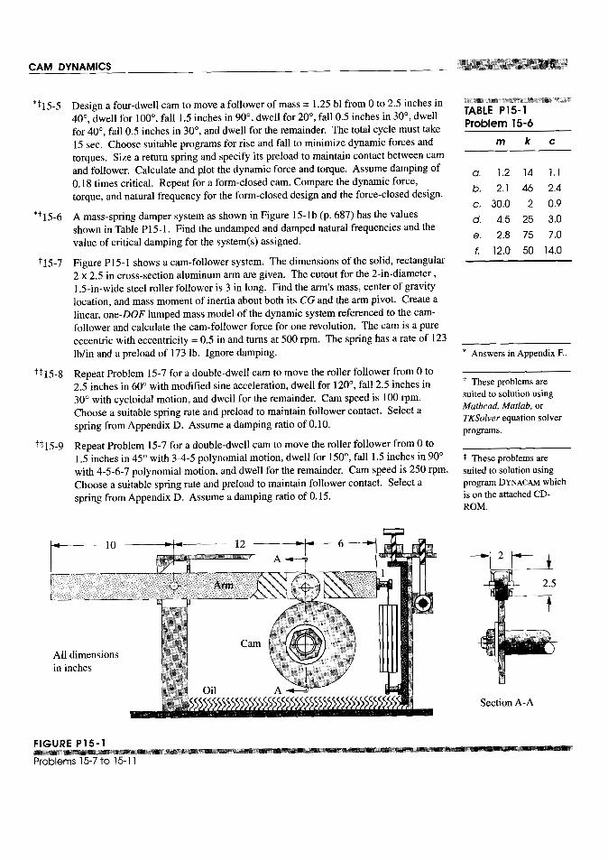


16.0 INTRODUCTION
Of all the myriad activities that the practicing engineer engages in, the one that is at oncethe most challenging and potentially the most satisfying is that of design. Doing calcula-tions to analyze a clearly defined and structured problem, no matter how complex, maybe difficult, but the exercise of creating something from scratch, to solve a problem that isoften poorly defined, is very difficult. The sheer pleasure and joy at conceiving a viablesolution to such a design problem is one of life's great satisfactions for anyone, engineeror not. The preceding chapters have attempted to present the particular subject matter ina way and context that will not only enhance the student's fundamental understanding ofthe topic but also encourage and promote his or her creative efforts toward the solutionof design problems.
As a closing to a book that began with a discussion of a design process in Chapter I,it is perhaps appropriate to present something of a "case study" of the design process toconclude the discussion. Some years ago, a very creative engineer of the author's ac-quaintance, George A. Wood Jr., heard a presentation by another creative engineer of theauthor's acquaintance, Keivan Towfigh, about one of his designs. Years later, Mr. Woodhimself wrote a short paper about creative engineering design in which he reconstructedMr. Towfigh's presumed creative process when designing the original invention. Both Mr.Wood and Mr. Towfigh have kindly consented to the reproduction of that paper here. Itserves, in this author's opinion, as an excellent example and model for the student of en-gineering design to consider when pursuing his or her own design career.
717
16.1 A DESIGN CASE STUDY
Educating for Creativity in Engineering[1]
by GEORGE A. WOOD JR.
One facet of engineering, as it is practiced in industry, is the creative process. Let usdefine creativity as Rollo May does in his book, The Courage to CreateJ21 It is "the pro-cess of bringing something new into being." Much of engineering has little to do withcreativity in its fullest sense. Many engineers choose not to enter into creative enterprise,but prefer the realms of analysis, testing and product or process refinement. Manyoth-ers find their satisfaction in management or business roles and are thus removed fromengineering creativity as we shall discuss it here.
From the outset, I wish to note that the less creative endeavors are no less importantor satisfying to many engineers than is the creative experience to those of us with the willto create. It would be a false goal for all engineering schools to assume that their pur-pose was to make all would-be engineers creative and that their success should be mea-sured by the "creative quotient" of their graduates.
On the other hand, for the student who has a creative nature, a life of high adven-ture awaits if he can find himself in an academic environment which recognizes his needs,enhances his abilities and prepares him for a place in industry where his potential can berealized.
In this talk I will review the creative process as I have known it personally and wit-nessed it in others. Then I shall attempt to indicate those aspects of my training thatseemed to prepare me best for a creative role and how this knowledge and these attitudestoward a career in engineering might be reinforced in today's schools and colleges.
During a career of almost thirty years as a machine designer, I have seen and beena part of a number of creative moments. These stand as the high points of my workinglife. When I have been the creator I have felt great elation and immense satisfaction.When I have been with others at their creative moments I have felt and been buoyed upby their delight. To me, the creative moment is the greatest reward that the profession ofengineering gives.
Let me recount an experience of eight years ago when I heard a paper given by a cre-ative man about an immensely creative moment. At the First Applied Mechanisms Con-ference in Tulsa, Oklahoma, was a paper entitled The Four-Bar Linkage as an Adjust-ment MechanismJ31 It was nestled between two "how to do it" academic papers withgraphs and equations of interest to engineers in the analysis of their mechanism problems.This paper contained only one very elementary equation and five simple illustrative fig-ures; yet, I remember it now more clearly than any other paper I have ever heard at mech-anism conferences. The author was Keivan Towfigh and he described the application ofthe geometric characteristics of the instant center of the coupler of afour bar mechanism.

His problem had been to provide a simple rotational adjustment for the oscillatingmirror of an optical galvanometer. To accomplish this, he was required to rotate theentire galvanometer assembly about an axis through the center of the mirror and per-pendicular to the pivot axis of the mirror. High rigidity of the system after adjustmentwas essential with very limited space available and low cost required, since up to six-teen of these galvanometer units were used in the complete instrument.
His solution was to mount the galvanometer elements on the coupler link of a one-piece, flexure hinged, plastic four bar mechanism so designed that the mirror center wasat the instant center of the linkage at the midpoint of its adjustment. (See Fig 4.) It is aboutthis particular geometric point (see Fig 1.) That pure rotation occurs and with properselection of linkage dimensions this condition of rotation without translation could bemade to hold sufficiently accurately for the adjustment angles required.
Unfortunately, this paper was not given the top prize by thejudges of the conference. Yet,it was, indirectly, a description of an outstandingly creative moment in the life of a creativeman.
Let us look at this paper together and build the steps through which the author prob-ably progressed in the achievement of his goal. I have never seen Mr. Towfigh since, andI shall therefore describe a generalized creative process which may be incorrect in somedetails but which, I am sure, is surprisingly close to the actual story he would tell.
The galvanometer problem was presented to Mr. Towfigh by his management. Itwas, no doubt, phrased something like this: "In our new model, we must improve thestability of the adjustment of the equipment but keep the cost down. Space is critical andlow weight is too. The overall design must be cleaned up, since customers like modern,slim-styled equipment and we' lllose sales to others if we don't keep ahead of them on allpoints. Our industrial designer has this sketch that all of us in sales like and within whichyou should be able to make the mechanism fit. "
Then followed a list of specifications the mechanism must meet, a time when the newmodel should be in production and, of course, the request for some new feature that wouldresult in a strong competitive edge in the marketplace.
I wish to point out that the galvanometer adjustment was probably only one hoped-for improvement among many others. The budget and time allowed were little more thanenough needed for conventional redesign, since this cost must be covered by the expect-ed sales of the resulting instrument. For every thousand dollars spent in engineering, anequivalent increase in sales or reduction in manufacturing cost must be realized at agreater level than the money will bring if invested somewhere else.
In approaching this project, Mr. Towfigh had to have a complete knowledge of theequipment he was designing. He had to have run the earlier models himself. He must (research)have adjusted the mirrors of existing machines many times. He had to be able to visualizethe function of each element in the equipment in its most basic form.

Secondly, he had to ask himself (as if he were the customer) what operational andmaintenance requirements wouldfrustrate him most. He had to determine which of thesemight be improved within the design time available. In this case he focused on the mirror
(ideation) adjustment. He considered the requirement of rotation without translation. He deter-mined the maximum angles that would be necessary and the allowable translation thatwould not affect the practical accuracy of the equipment. He recognized the desirabilityof a one screw adjustment. He spent a few hours thinking of all the ways he had seen of
(frustration) rotating an assembly about an arbitrary point. He kept rejecting each solution as it cameto him as he felt, in each case, that there was a better way. His ideas had too many parts,involved slides, pivots, too many screws, were too vibration sensitive or too large.
(incu bati on)He thought about the problem that evening and at other times while he proceeded
with the design of other aspects of the machine. He came back to the problem severaltimes during the next few days. His design time was running out. He was a mechanism
(Eureka!) specialist and visualized a host of cranks and bars moving the mirrors. Then one day,probably after a period when he had turned his attention elsewhere, on rethinking of the

adjustment device an image of the system based on one of the elementary characteristicsof a four bar mechanism came to him.
I feel certain that this was a visual image, as clear as a drawing on paper. It wasprobably not complete but involved two inspirations. First was the characteristics of theinstant center. (See Figs 1,2,3.) Second was the use of flexure hinge joints which led toa one-piece plastic molding. (See Fig 4.) I am sure that at this moment he had a feelingthat this solution was right. He knew it with certainty. The whole of his engineeringbackground told him. He was elated. He was filled with joy. His pleasure was not be-cause of the knowledge that his superiors would be impressed or that his security in thecompany would be enhanced. It was the joy of personal victory, the awareness that hehad conquered.
The creative process has been documented before by many others far more quali-fied to analyze the working of the human mind than I. Yet I would like to address, for theremaining minutes, how education can enhance this process and help more engineers, de-signers and draftsmen extend their creative potential.
The key elements I see in creativity that have greatest bearing on the quality thatresults from the creative effort are visualization and basic knowledge that gives strengthto the feeling that the right solution has been achieved. There is no doubt in my mind thatthe fundamental mechanical principles that apply in the area in which the creative effortis being made must be vivid in the mind of the creator. The words that he was given inschool must describe real elements that have physical, visual significance. F = ma mustbring a picture to his mind vivid enough to touch.
If a person decides to be a designer, his training should instill in him a continuingcuriosity to know how each machine he sees works. He must note its elements and men-tally see them function together even when they are not moving. I feel that this kind ofsolid, basic knowledge couples with physical experience to build ever more critical levels .at which one accepts a tentative solution as "right." (analysIs)
It should be noted that there have been times for all of us when the inspired "right"solution has proven wrong in the long run. That this happens does not detract from theprocess but indicates that creativity is based on learning and that failures build toward afirmer judgment base as the engineer matures. These failure periods are only negative, inthe growth of a young engineer, when they result in the fear to accept a new challenge andbeget excessive caution which then stifles the repetition of the creative process.
What would seem the most significant aspects of an engineering curriculum to helpthe potentially creative student develop into a truly creative engineer?
First is a solid, basic knowledge in physics, mathematics, chemistry and those sub-jects relating to his area of interest. These fundamentals should have physical meaningto the student and a vividness that permits him to explain his thoughts to the untrainedlayman. All too often technical words are used to cover cloudy concepts. They serve theego of the user instead of the education of the listener.

Second is the growth of the student's ability to visualize. The creative designer mustbe able to develop a mental image of that which he is inventing. The editor of the bookSeeing with the Mind's Eye/41 by Samuels and Samuels, says in the preface:
"... visualization is the way we think. Before words, images were. Visualization is the heartof the bio-computer. The human brain programs and self-programs through its images. Ridinga bicycle, driving a car, learning to read, baking a cake, playing golf - all skills are acquiredthrough the image making process. Visualization is the ultimate consciousness tool."
Obviously, the creator of new machines or products must excel in this area.
To me, a course in Descriptive Geometry is one part of an engineer's training thatenhances one's ability to visualize theoretical concepts and graphically reproduce theresult. This ability is essential when one sets out to design a piece of new equipment.First, he visualizes a series of complete machines with gaps where the problem or un-known areas are. During this time, a number of directions the development could takebegin toform. The best of these images are recorded on paper and then are reviewed withthose around him until, finally, a basic concept emerges.
The third element is the building of the student's knowledge of what can be or hasbeen done by others with different specialized knowledge than he has. This is the area towhich experience will add throughout his career as long as he maintains an enthusiasticcuriosity. Creative engineering is a building process. No one can develop a new conceptinvolving principles about which he has no knowledge. The creative engineer looks atproblems in the light of what he has seen, learned and experienced and sees new ways forcombining these to fill a new need.
Fourth is the development of the ability of the student to communicate his knowledgeto others. This communication must involve not only skills with the techniques used bytechnical people but must also include the ability to share engineering concepts with un-trained shop workers, business people and the general public. The engineer will seldomgain the opportunity to develop a concept if he cannot pass on to those around him hisenthusiasm and confidence in the idea. Frequently, truly ingenious ideas are lost becausethe creator cannot transfer his vivid image to those who might finance or market it.
Fifth is the development of a student's knowledge of the physical result of engineer-ing. The more he can see real machines doing real work, the more creative he can be asa designer. The engineering student should be required to run tools, make products, ad-just machinery and visit factories. It is through this type of experience that judgementgrows as to what makes a good machine, when approximation will suffice and where op-timization should halt.
It is often said that there has been so much theoretical development in engineeringduring the past few decades that the colleges and universities do not have time for thebasics I have outlined above. It is suggested that industry should fill in the practice areasthat colleges have no time for, so that the student can be exposed to the latest technology.To some degree I understand and sympathize with this approach, but Ifeel that there is anegative side that needs to be recognized. If a potentially creative engineer leaves col-
lege without the means to achieve some creative success as he enters his first job, his en-thusiasm for creative effort is frustrated and his interest sapped long before the most en-lightened company can fill in the basics. Therefore, a result of the "basics later" approachoften is to remove from the gifted engineering student the means to express himself visu-ally and physically. Machine design tasks therefore become the domain of the graduatesof technical and trade schools and the creative contribution by many a brilliant universi-ty student to products that could make all our lives richer is lost.
As I said at the start, not all engineering students have the desire, drive and enthusi-asm that are essential to creative effort. Yet I feel deeply the need for the enhancement ofthe potential of those who do. That expanding technology makes course decisions diffi-cult for both student and professor is certainly true. The forefront of academic thoughthas a compelling attraction for both the teacher and the learner. Yet I feel that the devel-opment of strong basic knowledge, the abilities to visualize, to communicate, to respectwhat has been done, to see and feel real machinery, need not exclude or be excluded bythe excitement of the new. I believe that there is a curriculum balance that can beachieved which will enhance the latent creativity in all engineering and science students.It can give a firm basis for those who look towards a career of mechanical invention andstill include the excitement of new technology.
I hope that this discussion may help in generating thought and providing some con-structive suggestions that may lead more engineering students to find the immense satis-faction of the creative moment in the industrial environment. In writing this paper I havespent considerable time reflecting on my years in engineering and I would close with thefollowing thought. For those of us who have known such times during our careers, thesuccessful culminations of creative efforts stand among our most joyous hours.


In addition to the student version of the commercial simulation program Working Mod-el, there are seven custom computer programs provided on the CD-ROM with this text:programs FOURBAR,FIVEBAR,SIXBAR,SLIDER,MATRIX,DYNACAM,and ENGINE.Theseare student editions of the programs. Professional versions with extended capabilities arealso available. Contact the author at [email protected] or visit his faculty page at the website http://www.wpi.eduJ for more information. Programs FOURBAR,FrVEBAR,SIXBAR,and SLIDERare based on the mathematics derived in Chapters 4 to 7 and 10 to 11 and usethe equations presented therein to solve for position, velocity, and acceleration in linkag-es of the variety described in the particular program's name. Program DYNACAMis a earndesign program based on the mathematics derived in Chapters 8 and 15. Program EN-GINEis based on the mathematics derived in Chapters 13 and 14. Program MATRIXis ageneral linear simultaneous equation solver. All have similar choices for display of out-put data in the form of tables and plots. All the programs are designed to be user friendlyand reasonably "crashproof." The author encourages users to email reports of any "bugs"or problems encountered in their use to him at [email protected].
Learning Tools
All the custom programs provided with this text are designed to be learning tools to aidin the understanding of the relevant subject matter and are specifically not intended to
725

be used for commercial purposes in the design of hardware and should not be so used.It is quite possible to obtain inappropriate (but mathematically correct) results to anyproblem solved with these programs, due to incorrect or inappropriate input of data. Inother words, the user is expected to understand the kinematic and dynamic theory un-derlying the program's structure and to also understand the mathematics on which theprogram's algorithms are based. This information on the underlying theory and mathe-matics is derived and described in the noted chapters of this text. Most equations usedin the programs are presented or derived in this textbook.
Disclaimer
Commercial software for use in design or analysis needs to have built-in safeguardsagainst the possibility of the user providing incorrect, inappropriate, or ridiculous valuesfor input variables, in order to guard against erroneous results due to user ignorance orinexperience. The student editions of the custom programs provided with this textare not commercial software and deliberately do not contain such safeguardsagainst improper input data, on the premise that to do so would "short circuit" the stu-dent's learning process. We learn most from our failures. These programs provide a con-sequence- free environment to explore failure of your designs "on paper" and in the pro-cess come to a more thorough and complete understanding of the subject matter. Theauthor and publisher are not responsible for any damages which may result fromthe use or misuse of these programs.
Brute Force and Ignorance
The very rapid computation speed of these programs allows the student to explore a muchlarger number and variety of potential solutions to more realistic and comprehensive prob-lems than could be accomplished using only hand calculator solutions of these compli-cated systems of equations. This is both an advantage and a danger. The advantage isthat the student can use the programs like a "flight simulator" to "fly" potential designsolutions through their paces with no consequences from a "crash" of the design not yetbuilt. If the student diligently attempts to interpret the program's results and relate themto the relevant theory, a more thorough understanding of the kinematics and dynamics canresult. On the other hand, there is a great temptation to use these programs with "bruteforce and ignorance" (BFI) to somewhat randomly try solutions without regard to whatthe theory and equations are telling you and hope that somehow a usable solution will"pop out." The student who succumbs to this temptation will not obtain much benefitfrom the exercise and will probably have a poor design result. This situation is probablybest summed up in the following comment from a student who had suffered through thecourse in kinematics using these programs to design solutions to three project problemslike those listed at the end of Chapter 3.
. . . The computer, with its immense benefits for the engineer, can also be a hindrance ifone does not first develop a thorough understanding of the theory upon which a particu-lar program is based. An over-reliance on the computer can leave one "computer smart"and "engineering stupid." The BFI approach becomes increasingly tempting when it canbe employed with such ease .... BRIAN KIMBALL
Smart student! Use these computer programs wisely. Avoid Brute Force and Igno-rance! Engineer your solutions and understand the theory behind them.

A.l GENERAL INFORMATION
Hardware Requirements
These programs work on any computer that runs Windows 3.1, Windows 95, orWindows NT. Different versions of the programs are provided for each operating sys-tem. A CD-ROM drive is needed, as is a hard disk drive. If your computer does not reada CD-ROM, your school's computer center can probably convert it to a usable format for you.
Operating System Requirements
These custom programs are written in Microsoft Visual Basic and are compiled in twoversions: Pgmname16.exe for the Windows 3.1 (16 bit) operating system andPgmname32.exe for the Windows 95 and NT (32 bit) operating systems. Be sure to usethe version suitable to your computer's hardware and software.
Installing the Software
The CD-ROM contains the executable program files plus all necessary Dynamic LinkLibrary (DLL) and other ancillary files needed to run the programs. Run the SETUP filefrom the individual program's folder on the CD-ROM to automatically decompress andinstall all of its files on your hard drive. A folder and icon will be created with that pro-gram's name. The program can then be run by double clicking on the icon or on thePgmnamel6.exe or Pgmname32.exe file itself. In Windows 95 or NT the program namewill appear in the list under the Start button's Program menu after installation and canbe run from there.
How to Use This Manual
This manual is intended to be used while running the programs. To see a screen referredto, bring it up within the program to follow its discussion.
A.2 GENERAL PROGRAM OPERATION
All seven programs in the set have similar features and operate in a consistent way. Forexample, all printing and plotting functions are selected from identical screens commonto all programs. Opening and saving files are done identically in all programs. Thesecommon operations will be discussed in this section independent of the particular pro-gram. Later sections will address the unique features and operations of each program.
Note that student editions of these programs are supplied with this book at no chargeand carry a limited-term license restricted to use in course work for up to two semesters(9 months). If you continue to use the program after that time, you are expected to reg-ister it and pay the shareware fee defined on the Registration screen. If you wish to usethe program for the benefit of a company or for any commercial purpose, then you mustobtain the professional edition of the same program. The student editions are not to beused commercially. The professional editions typically offer more features than the stu-dent editions.

Running the Programs (All Programs)
At start-up, a splash screen appears which identifies the program version, revision num-ber, and revision date. Click the button labeled Start or press the Enter key to run theprogram. A Disclaimer screen next appears which defines the registered owner and al-lows the printing of a registration form if the software is as yet unregistered. A registra-tion form can be accessed and printed from this screen.
The next screen, the Title screen, allows the input of any user and/or project identi-fication desired. This information must be provided to proceed and is used to identifyall plots and printouts from this program session. The second box on the Title screen al-lows any desired file name to be supplied for storing data to disk. This name defaults toModell and may be changed at this screen and/or when later writing the data to disk.The third box allows the typing of a starting design number for the first design. Thisdesign number defaults to I and is automatically incremented each time you change thebasic design during this program session. It is used only to identify plots, data files, andprintouts so they can be grouped, if necessary, at a later date. When the Done button onthe Title screen is clicked, the Home screen appears.
The Home Screen (All Programs)
All program actions start and end at the Home screen which has several pull-down menusand buttons, some of which commands (File, New, Open, Save, Save As, Units, About,Plot, Print, Quit) are common to all programs. These will be described below.
General User Actions Possible Within a Program (All Programs)
The programs are constructed to allow operation from the keyboard or the mouse or withany combination of both input devices. Selections can be made either with the mouseor, if a button is highlighted (showing a dotted square within the button), the Enter keywill activate the button as if it had been clicked with the mouse. Text boxes are providedwhere you need to type in data. These have a yellow background. In general, what youtype in any text box is not accepted until you hit the Enter key or move off that box withthe Tab key or the mouse. This allows you to retype or erase with no effect until youleave the text box. You can move between available input fields with the Tab key (andbackup with Shift-Tab) on most screens. If you are in doubt as to the order in which toinput the data on any screen, try using the Tab key as it will take you to each needed entryfield in a sensible order. You can then type or mouse click to input the desired data inthat field. Remember that a yellow background means typed input data is expected.Boxes with a cyan background provide information back to you but cannot be typed in.
Other information required from you is selected from drop-down menus or lists.These have a white background.· Some lists allow you to type in a value different thanany provided in the available list of selections. If you type an inappropriate response, itwill simply ignore you or choose the closest value to your request. Typing the first fewletters of a listed selection will sometimes cause it to be selected. Double clicking on aselectable item in a list will often provide a shortcut.

Units (All Programs)
The Units menu defines several units systems to choose from. Note that all programswork entirely in pure numbers without regard to units. It is your responsibility to ensurethat the data as input are in some consistent units system. No units conversion is donewithin the programs. The Units menu selection that you make has only one effect,namely to change the labels displayed on various input and output parameters within theprogram. You mix units systems at your own peril.
Examples (Most Programs)
Most of the programs have an Examples pull-down menu on the Home screen which pro-vides some number of example mechanisms that will demonstrate the program's capa-bility. Selecting an example from this menu will cause calculation of the mechanism andopen a screen to allow viewing the results. In some cases you may need to hit a buttonmarked Calculate, Run, or Animate on the presented screen to see the results. Some pro-grams also provide access to examples from various screens.
Creating New, Saving, and Opening Files (File - All Programs)
The standard Windows functions for creating new files, saving your work to disk, andopening a previously saved file are all accessible from the pull-down menu labeled Fileon each program's Home screen. Selecting New from this menu will zero any data youmay have already created within the program, but before doing so will give warning andprompt you to save the data to disk.
The Save and Save As selections on the File menu prompt you to provide a file nameand disk location to save your current model data to disk. The data are saved in a cus-tom format and with a three-character suffix unique to the particular program. Youshould use the recommended suffix on these files as that will allow the program to seethem on the disk when you want to open them later. If you forget to add the suffix whensaving a file, you can still recover the file.
Selecting Open from the File menu prompts you to pick a file from those availablein the disk directory that you choose. If you do not see any files with the program's suf-fix, use the pull-down menu within the Open File dialog box to choose Show All Filesand you will then see them. They will read into the program properly with or withoutthe suffix in their name as long as they were saved from the same program. If you are aformer user of the DOS versions of these programs, files saved from the older version ofa given program can also be opened in its Windows version, though they will not have asmuch information as is needed in the new programs.
Copying Screens to Clipboard or Printer (Copy - All Programs)
Any screen can be copied as a graphic to the clipboard by using the standard Windowskeyboard combo of Alt-PrintScm. It will then be available for pasting into any compat-ible Windows program such as Word or Powerpoint that is running concurrently in Win-dows. Most screens also provide a button to dump the screen image to an attached laserprinter. However, the quality of that printed image may be less than could be obtained


CARTESIANPLOTS depict a dependent variable versus an independent variable oncartesian (x, y) axes. In these programs, the independent variable shown on the x axis maybe either time or angle, depending on the calculation choice made in the particular pro-gram. The variable for the y axis is selected from the plot menu. Angular velocities andtorques are vectors but are directed along the z axis in a two-dimensional system. So theirmagnitudes can be plotted on cartesian axes and compared because their directions areconstant, known, and the same.
POLAR PLOTS Plots of linear velocities, linear accelerations, and forces require adifferent treatment than the cartesian plots used for the angular vector parameters. Theirdirections are not the same and vary with time or input angle. One way to represent theselinear vectors is to make two cartesian plots, one for magnitude and one for angle of thevector at each time or angle step. Alternatively, the x and y components of the vector ateach time or angle step can be presented as a pair of cartesian plots. Either of these ap-proaches requires two plots per vector and has the disadvantage of being difficult to inter-pret. A better method for vectors that act on a moving point (such as a force on a movingpin) can be to make a polar plot with respect to a local, nonrotating axis coordinate sys-tem (LNCS) attached at the moving point. This local, nonrotating x, y axis system trans-lates with the point as it moves but remains always parallel to the global axis system X.Y.By plotting the vectors on this moving axis system we can see both their magnitude anddirection at each time or angle step, since we are attaching the roots of all the vectors tothe moving point at which they act.
In some of the programs, polar plots can be paused between the plotting of each vec-tor. Without a pause, the plot can occur too quickly for the eye to detect the order in whichthey are drawn. When a mouse click is required between the drawing of each vector, theirorder is easily seen. With each pause, the current value of the independent variable (timeor angle) as well as the magnitude and angle of the vector are displayed.
The programs also allow alternate presentations of polar plots, showing just the vec-tors, just the envelope of the path of the vector tips, or both. A plot that connects the tipsof the vectors with a line (its envelope) is sometimes called a hodograph.
SELECTING PLOT VARIABLES Choosing anyone of the four plot types from thePlot Type screen brings up a Plot Select screen which is essentially the same in all pro-grams. (See Figure A-3.) As with the Print Select screen, two arrangements for select-ing the functions to be plotted are provided, Preset Formats and Mix and Match. Theformer provides preselected collections of functions, and the latter allows you to selectup to four functions from those available on the pull-down menus. In some cases youwill also have to select the component of the function desired, i.e., x, y, mag, or angle.
PLOT ALIGNMENT Some of the Plot Select screens offer a choice of two furtherplot style variants labeled Aligned and Annotated. The aligned style places multiple plotsin exact phase relationship, one above the other. The annotated style does not align theplots but allows more variety in their display such as fills and grids. The data displayedis the same in each case.
COORDINATESYSTEMS For particular variables in some programs, a choice of co-ordinate system is provided for display of vector information in plots. The CoordinateSystem panel on the Plot Select screen will become active when one of these variables isselected. Then either the Global or Local button can be clicked. (It defaults to Global.)

GLOBAL COORDINATES The Global choice in the Coordinate System panel refersall angles to the XY axes of Figure A-6 (p. 737). For polar plots the vectors shown withthe Global choice actually are drawn in a local, nonrotating coordinate system (LNCS)that remains parallel to the global system such as Xl, YI at point A andx2, Y2 at point B inFigure A-I. The LNCS X2, Y2 at point B behaves in the same way as the LNCS Xl, YI atpoint A; that is, it travels with point B but remains parallel to the world coordinate sys-tem X,Y at all times.
LOCAL COORDINATES The coordinate system x',y' also travels with point B as itsorigin, but is embedded in link 4 and rotates with that link, continuously changing its ori-entation with respect to the global coordinate system X,Y making it an LRCS. Each linkhas such an LRCS but not all are shown in the figure. The Local choice in the CoordinateSystem panel uses the LRCS for each link to allow the plotting and printing of the tan-gential and radial components of acceleration or force on a link. This is of value if, forexample, a bending stress analysis of the link is wanted. The dynamic force componentsperpendicular to the link due to the product of the link mass and tangential accelerationwill create a bending moment in the link. The radial component will create tension orcompression.
PLOTTING Once your selections are made and are shown in the cyan boxes at thelower right of the Plot Select screen, the Done button will become available. Clicking itwill bring up the plots that you selected. Figure A-4 shows examples of the four plottypes available. From this Plot screen you may copy to the clipboard for pasting intoanother application or dump the Plot screen to a printer. The Select Another button re-turns you to the previous Plot Select screen. Done returns you to the Home screen.

The About Menu (All Programs)
The About pull-down menu on the Home screen will display a splash screen containinginformation on the edition and revision of your copy of the program. The Disclaimerand Registration form can also be accessed from this menu.
Exiting a Program (All Programs)
Choosing either the Quit button or Quit on the File pull-down menu on the Home screenwill exit the program. If the current data has not been saved since it was last changed, itwill prompt you to save the model using an appropriate suffix. In all cases, it will askyou to confirm that you want to quit. If you choose yes, the program will terminate andany unsaved data will be gone at that point.

Support (All Programs)
Please notify the author of any bugs via email to [email protected].
A.3 PROGRAM FOURBAR
FOURBARfor Windows is a linkage design and analysis program intended for use by stu-dents, engineers and other professionals who are knowledgeable in or are learning theart and science of linkage design. It is assumed that the user knows how to determinewhether a linkage design is good or bad and whether it is suitable for the application forwhich it is intended. The program will calculate the kinematic and dynamic data associ-ated with any linkage design, but cannot substitute for the engineering judgment of theuser. The linkage theory and mathematics on which this program is based are document-ed in Chapters 4 to 7, 10, and 11 of this textbook. Please consult them for explanationsof the theory and mathematics involved.
The FOURBAR Home Screen
Initially, only the Input and Quit buttons are active on the Home screen. Typically, youwill start a linkage design with the Input button, but for a quick look at a linkage as drawnby the program, one of the examples under the Example pull-down menu can be select-ed and it will draw a linkage. If you activate one of these examples, when you returnfrom the Animate screen you will find all the other buttons on the Home screen to be ac-tive. We will address each of these buttons in due course below.
Input Data (FOURBAR Input Screen)
Figure A-5 defines the input parameters, link numbering, and the axis system used in pro-gram FOURBAR. The link lengths needed are ground link 1, input link 2, coupler link 3,and output link 4, defined by their pin-to-pin distances and labeled a, b, c, d in the figure.The X axis is constrained to lie along link 1, defined by the instant centers h 2 and h 4
which are also labeled, respectively, 02 and 04 in the figure. Instant center h ;, the dri~-er crank pivot, is the origin of the global coordinate system.
It might seem overly restrictive to force the X axis to lie on link 1 in this "alignedsystem." Many linkages will have their ground link at some angle other than zero. How-ever, reorienting the linkage after designing and analyzing it merely involves rotating thepiece of paper on which it is drawn to the desired final angle of the ground link. Moreformally, it means a rotation of the coordinate system through the negative of the angleof the ground link. In effect, the actual final angle of the ground link must be subtractedfrom all angles of links and vectors calculated in the aligned axis system.
In addition to the link lengths, you must supply the location of one coupler point onlink 3 to find that point's coupler curve positions, velocities, and accelerations. This pointis located by a position vector rooted at h,3 (point A) and directed to the coupler point Pof interest which can be anywhere on link 3. The program requires that you input the polarcoordinates of this vector which are labeled p and 03 in Figure A-5. The program asks forthe distance from h,3 to the coupler point, which is p, and the angle the coupler point

makes with link 3 which is 03. Note that angle 03 is not referenced to either the globalcoordinate system (GCS) X,Y or to the local nonrotating coordinate system (LNCS) x,yat point A. Rather, it is referenced to the line AB which is the pin-to-pin edge of link 3(LRCS). Angle 03 is a property of link 3 and is embedded in it. The angle which locatesvector RCA in the x,y coordinate system is the sum of angle 03 and angle 83. This additionis done in the program, after 83 is calculated for each position of the input crank. Also seeSection 4.5 (p. 152). The coordinate system, dimensions, angles, and nomenclature inFigure A-5 are consistent with those of Figure 4-6 (p. 154) which were used in the deri-vation of the equations used in program FOURBAR.
Calculation (FOURBAR,FIVEBAR,SIXBAR,and SLIDERInput Screens)
Basic data for a linkage design is defined on the Input screen shown in Figure A-6, whichis activated by selecting the Input button on the Home screen. When you open this screenfor the first time, it will have default data for all parameters. The linkage geometry isdefined in the Linkage Data panel on the left side of the screen. You may change theseby typing over the data in the yellow text boxes.
The open or crossed circuit of the linkage is selected in a panel at the lower left ofthe screen in Figure A-6. Select the type of calculation desired, one of Angle Steps, TimeSteps, or One Position from the Calculation Mode in the upper-right panel. The start,finish, and delta step information is different for each of these calculation methods, andthe input text box labels in the Initial Conditions panel will change based on your choice.Type the desired initial, delta, and final conditions as desired.
ONE POSITION will calculate position, velocity, and acceleration for anyone spec-ified input position 82, input angular velocity (02, and angular acceleration «2·
ANGLESTEPS assumes that the angular acceleration «2 of input link 2 is zero, mak-ing Wz constant. The values of initial and final crank angle 82, angle step ~82, and theconstant input crank velocity (02 are requested. The program will compute all linkage pa-
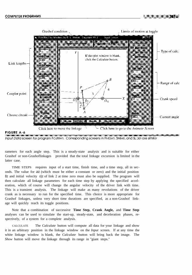
rameters for each angle step. This is a steady-state analysis and is suitable for eitherGrashof or non-Grashoflinkages provided that the total linkage excursion is limited in thelatter case.
TIME STEPS requires input of a start time, finish time, and a time step, all in sec-onds. The value for az (which must be either a constant or zero) and the initial position8z and initial velocity o)z of link 2 at time zero must also be supplied. The program willthen calculate all linkage parameters for each time step by applying the specified accel-eration, which of course will change the angular velocity of the driver link with time.This is a transient analysis. The linkage will make as many revolutions of the drivercrank as is necessary to run for the specified time. This choice is more appropriate forGrashof linkages, unless very short time durations are specified, as a non-Grashof link-age will quickly reach its toggle positions.
Note that a combination of successive Time Step, Crank Angle, and Time Stepanalyses can be used to simulate the start-up, steady-state, and deceleration phases, re-spectively, of a system for a complete analysis.
CALCULATE The Calculate button will compute all data for your linkage and showit in an arbitrary position in the linkage window on the Input screen. If at any time thewhite linkage window is blank, the Calculate button will bring back the image. TheShow button will move the linkage through its range in "giant steps."

After you have calculated the linkage, the Animate and Done buttons on the Inputscreen will become available. The Animate button takes you to the Animate screen whereyou can run the linkage through any range of motion to observe its behavior. You canalso change any of the linkage parameters on the Animate screen and then recalculate theresults there with the Recalc button. The Done button on either the Input or Animatescreen returns you to the Home screen. The Plot and Print buttons will now be availableas well as the Animate button which will send you to the Animate screen.
CALCULATION ERRORS If a position is encountered which cannot be reached bythe links (in either the angle step or time step calculations), the mathematical result willbe an attempt to take the square root of a negative number. The program will then showa dialog box with the message Links do not connect for Theta2=xx and present threechoices: Abort, Retry, or Ignore. Abort will terminate the calculation at this step and re-turn you to the Input screen. Retry will set the calculated parameters to zero at the cur-rent position and attempt to continue the computation at the next step, reporting succes-sive problems as they occur. Ignore will continue the calculation for the entire excursion,setting the calculated parameters to zero at any subsequent positions with problems butwill not present any further error messages. If a linkage is non-Grashof and you requestcalculation for angles that it cannot reach, then you will trip this error sequence. Choos-ing Ignore will force the calculation to completion, and you can then observe the possiblemotions of the linkage in the linkage window of the Input screen with the Show button.
GRASHOF CONDITION Once the calculation is done, the linkage's Grashof condi-tion is displayed in a panel at the top left of the screen. If the linkage is non-Grashof, theangles at which it reaches toggle positions are displayed in a second panel at top right.This information can be used to reset the initial conditions to avoid tripping the "linkscannot connect" error.
Animation (FOURBAR)
The Animate button on the Home screen brings up the Animate screen as shown in FigureA-7. Its Run button activates the linkage and runs it through the range of motion definedin its most recent calculation. The Grashof condition is reported at the upper right comerof the screen. The number of cycles for the animation can be typed in the Cycles box atthe lower right of the screen.
A time delay (defaulted to 0) can be set with a drop-down menu below the Cycles box.Any number of cycles not on its list can be typed in the box. This time-delay feature isprovided to accommodate variations in speed among computers. If your computer is veryfast, the animation may occur too rapidly to be seen. If so, selecting larger positive num-bers for the time delay will slow the animation. For slow computers, negative numberswill speed the animation to a degree but can make it jerky. The Step button moves thelinkage one increment of the independent variable at a time.
Text boxes in the Linkage Data panel allow the linkage geometry to be changed with-out returning to the Input screen. The initial conditions can be redefined in the panel onthe left of this screen. The Open-Crossed selection can be switched, but the CalculationType can only be changed on the Input screen. After any such change, the linkage mustbe recalculated with the Recalc button and then rerun.

Two panels at the top center of the Animate screen provide switches to change theanimation display. In the Show Curves panel, displays of Links, Coupler Path, and Cen-trades can be turned on and off in subsequent animations.
CENTRODES Only the FOURBARprogram calculates and draws the fixed and mov-ing centrodes (the loci of the instant centers as defined in Section 6.5 (p. 263) and shownin Figure 6-15a, p. 266). Different colors are used to distinguish the fixed from the mov-ing centrode. The centrodes are drawn with their point of common tangency located atthe first position calculated. Thus, you can orient them anywhere by your choice of startangle for the calculation.
AUTOSCALE can be turned on or off in the Animation Settings panel. The linkageanimation plot is normally autoscaled to fit the screen based on the size of the linkageand its coupler curves (but not of the centrodes as they can go to infinity). You may wantto turn off autoscaling when you wish to print two plots of different linkages at the samescale for later manual superposition. Turning off auto scaling will retain the most recentscale factor used. When on, it will rescale each plot to fit the screen.
TRACE Turning Trace on keeps all positions of the linkage visible on the screen sothat the pattern of motion can be seen. Turning Trace off erases all prior positions, show-ing only the current position as it cycles the linkage through all positions giving a dynam-ic view of linkage behavior.


The FOURBARBalance screen in Figure A-lO displays two mini-plots that superposethe shaking forces and shaking torques before and after balancing. Effects on the shak-ing force and torque from changes in the amount of balance mass-radius product placedon each link can be immediately seen in these plots. The energy in each pulse of thetorque-time curve is also displayed in a sidebar on the right of this screen for use in aflywheel sizing calculation. See Section 11.11 (p. 548) for a discussion of the meaningand use of these data. The program calculates a smoothed torque function by multiply-ing the raw torque by the coefficient of fluctuation specified in the box at lower left.
Cognates (FOURBAR Only)
The Cognates pull-down menu allows switching among the three cognates which createthe same coupler curve. Switching among them requires recalculation of all kinematicand dynamic parameters via the Input, Dynamics, and Balance buttons. The previouslyused mass property data is retained but can be changed easily by selecting the Dynamicsbutton. The Cayley Diagram menu pick under Cognates displays that diagram of allthree cognates. See Chapter 3. Whenever linkage data are changed on the Input Screenand recalculated, the program automatically calculates the dimensions of that linkage'stwo cognates. These can be switched to, calculated, and investigated at any time.
Synthesis (FOURBAR Only)
This pull-down menu allows selection of two- or three-position synthesis of a linkage,each with a choice of two methods. See Chapter 5 for a discussion of these methods andderivations of the equations used. When the linkage is synthesized, its link geometry isautomatically put into the input sheet and recalculation is then required.
Other
See Section A.2, General Program Operation (p. 727) for information on New, Open,Save, Save As, Plot, Print, Units, and Quit functions.
A.4 PROGRAM FIVE BAR
FIVEBARfor Windows is a linkage design and analysis program intended for use by stu-dents, engineers, and other professionals who are knowledgeable in or are learning theart and science of linkage design. It is assumed that the user knows how to determinewhether a linkage design is good or bad and whether it is suitable for the application forwhich it is intended. The program will calculate the kinematic and dynamic data associ-ated with any geared fivebar linkage design, but cannot substitute for the engineeringjudgment of the user. The linkage theory and mathematics on which this program isbased are documented in Chapters 4 to 7, and 11 of this textbook. Please consult themfor explanations of the theory and mathematics involved.
The FIVEBAR Home Screen
Initially, only the Input and Quit buttons are active on the Home screen. Typically, youwill start a linkage design with the Input button, but for a quick look at a linkage as drawn


Basic data for the five bar linkage is defined on the Input screen which is similar tothat for FOURBARshown in Figure A-6 (p. 737). The Input screen is activated by select-ing the Input button on the Home screen. When you open this screen for the first time, itwill have default data for all link parameters. You may change any of these by typingover the data in the yellow text boxes.
Select the type of calculation desired in the upper right comer of the screen, one ofAngle Steps, Time Steps, or One Position. The Calculate button will compute all datafor your linkage and show it in an arbitrary position on the screen. If the white linkagedisplay window is blank, the Calculate button will bring back the image. See the dis-cussion of calculations for the FOURBARprogram in Section A.3 (p. 735). They are sim-ilar in FIVEBAR.
After you have calculated the linkage, the Animate and Done buttons on the Inputscreen will become available. Animate takes you to the Animate screen where you canrun the linkage through any range of motion to observe its behavior. You can also changeany of the linkage parameters on the Animate screen and then recalculate the results withthe Recalc button. The Done button on either the Input or Animate screen returns you tothe Home screen. The Plot and Print buttons will now be available as well as the Ani-mate button which returns you to the Animate screen.
Animation (FIVEBAR)
In program FrVEBAR,the Animation screen and its features are essentially similar tothose of program FOURBAR. The only exception is the lack of a centrode selection inFIVEBAR.See the Animation discussion for FOURBARin Section A-3 for more informa-tion.
Dynamics (FIVEBAR Dynamics Screen)
Input data for dynamics calculation in FIVEBARare similar to that for program FOURBARwith the addition of one more link. However, linkage balancing is not available in FIVE-BAR. See the discussion of dynamics calculations for program FOURBARin Section A-3for more information.
Other
See Section A.2, General Program Operation (p. 727) for information on New, Open,Save, Save As, Plot, Print, Units, and Quit functions.
A.5 PROGRAM SIXBAR
SIxBARfor Windows is a linkage design and analysis program intended for use by stu-dents, engineers, and other professionals who are knowledgeable in or are learning theart and science of linkage design. It is assumed that the user knows how to determinewhether a linkage design is good or bad and whether it is suitable for the application forwhich it is intended. The program will calculate the kinematic and dynamic data associ-ated with any linkage design but cannot substitute for the engineering judgment of theuser. The linkage theory and mathematics on which this program is based are document-

The SIXBAR Home Screen
Initially, only the Input and Quit buttons are active on the Home screen. Typically, youwill start a linkage design with the Input button, but for a quick look at a linkage as drawnby the program, one of the examples under the Example pull-down menu can be select-ed and it will draw a linkage. If you activate one of these examples, when you returnfrom the Animate screen you will find all the other buttons on the Home screen to be ac-tive. We will address each of these buttons in due course below.
The Home screen's Examples pull-down menu includes both Watt's and Roberts'straight-line fourbar linkage stages driven by dyads (making them sixbars), a single-dwellsixbar linkage similar to that of Example 3-13 (p. 126) and Figure 3-31 (p. 127), and adouble-dwell sixbar linkage that uses an alternate approach to that of Example 3-14 (p.130) and Figure 3-32 (p. 129).
Input Data (SIXBARInput Screen)
Much of the basic data for the linkage design is defined on the Input screen which isactivated by selecting the Input button on the Home screen. When you open this screenfor the first time, it will have default data for all link parameters. You may change anyof these by typing over the data in the yellow text boxes. A choice of Watt's or Stephen-son's linkage must be made on the Input screen. The link information differs for theWatt's and Stephenson's linkages.
WATT'S II LINKAGE For the Watt's linkage (Figure A-12) the stage 1 data is:crank, first coupler, first rocker, and ground link segment from instant centers h,2 to h,4.These correspond to links 2, 3a, 4a, and la, respectively, as labeled in the Figure A-12.The stage 2 data are: second crank, second coupler, second rocker, corresponding respec-tively to links 4b, 5a, and 6 in Figure A-12. The angle 04 that the second crank (4b)makes with the first rocker (4a) is also requested. Note that this angle obeys the right-hand rule as do all angles in these programs.
Two coupler points are allowed to be defined in this linkage, one on link 3 and oneon link 5. The method of location is by polar coordinates of a position vector embeddedin the link as was done for the fourbar and fivebar linkages. The first coupler point C ison link 3 and is defined in the same way as in FOURBAR. Program SrxBAR requires the

length (3c) of its position vector RCA and the angle <>3 which that vector makes with line3a in Figure A-12. The second coupler point F is on link 5 and is defined with a positionvector RFD rooted at instant center 14,S' The program requires the length (5c) of this po-sition vector RFD and the angle <>s which that vector makes with line 5a. The X and Ycomponents of the location of the third fixed pivot 11,6 are also needed. These are withrespect to the global X, Y axis system whose origin is at h,2.
STEPHENSON'S III LINKAGE The stage I data for the Stephenson's linkage issimilar to that of the Watt's linkage. The first stage's crank, first coupler, first rocker,and ground link segment from instant centers 11,2 to 11,4 correspond to links 2, 3a, 4, andla, respectively, in Figure A-13. The link lengths in stage 2 of the linkage are: secondcoupler and second rocker corresponding, respectively, to links 5a and 6 in Figure A-B.
Note that, unlike the Watt's linkage, there is no "second crank" in the Stephenson'slinkage because the second stage is driven by the coupler (link 3) of the first stage. Inthis program link 5 is constrained to be connected to link 3 at link 3's defined couplerpoint C which then becomes instant center h,s. The data for this are requested in similarformat to the Watt's linkage, namely, the length of the position vector RCA (line 3c) andits angle <>3. The second coupler point location on link 5 is defined, as before, by posi-tion vector RFc with length 5c and angle <>s.
The X and Y components of the location of the third fixed pivot 11,6 are required.These are with respect to the global X,Y axis system.
Select the type of calculation desired in the upper right comer of the screen, one ofAngle Steps, Time Steps, or One Position. The Calculate button will compute all datafor your linkage and show it in an arbitrary position on the screen. If at any time the link-

age display window is blank, the Calculate button will bring back the image. See thedescription of calculations for program FOURBARin Section A.3 (p. 735). They are sim-ilar in SIXBAR.
After you have calculated the linkage, the Animate and Done buttons on the Inputscreen will become available. Animate takes you to the Animate screen where you canrun the linkage through any range of motion to observe its behavior. You can also changeany of the linkage parameters on the Animate screen and then recalculate the results withthe Recalc button. The Done button on either the Input or Animate screen returns you tothe Home screen. The Plot and Print buttons will now be available as well as the Ani-mate button which returns you to the Animate screen.
Animation (SIXBAR)
The Animation screen and its features in SIXBARare essentially similar to those of Pro-gram FOURBAR. The only exception is the lack of a Centrode selection in SIXBAR.Seethe Animation discussion for FOURBARin Section A.3 for more information.
Dynamics (SIXBARDynamics Screen)
Input data for dynamics calculation in SIXBARare similar to that for program FOURBARwith the addition of two links. See the discussion of dynamics calculations for programFOURBARin Section A.3 for more information.

Other
See Section A.2, General Program Operation (p. 727) for information on New, Open,Save, Save As, Plot, Print, Units, and Quit functions.
A.6 PROGRAM SLIDER
SLIDERfor Windows is a linkage design and analysis program intended for use by stu-dents, engineers, and other professionals who are knowledgeable in or are learning theart and science of linkage design. It is assumed that the user knows how to determinewhether a linkage design is good or bad and whether it is suitable for the application forwhich it is intended. The program will calculate the kinematic and dynamic data associ-ated with any linkage design, but cannot substitute for the engineering judgment of theuser. The linkage theory and mathematics on which this program is based are document-ed in Chapters 4 to 10, and 11 of this textbook. Please consult them for explanations ofthe theory and mathematics involved.
The Slider Home Screen
Initially, only the Input and Quit buttons are active on the Home screen. Typically, youwill start a linkage design with the Input button, but for a quick look at a linkage as drawnby the program, one of the examples under the Example pull-down menu can be select-ed and it will draw a linkage. If you activate one of these examples, when you returnfrom the Animate screen you will find all the other buttons on the Home screen to be ac-tive. We will address each of these buttons below.
Input Data (SUDERInput Screen)
Basic data for the sixbar linkage is defined on the Input screen, which is activated byselecting the Input button on the Home screen. When you open this screen for the firsttime, it will have default data for all link parameters. You may change any of these bytyping over the data in the yellow text boxes.
Figure A-14 defines the input parameters for the fourbar slider-crank linkage. Thelink lengths needed are input link 2 and coupler link 3, defined by their pin-to-pin distanc-es and labeled a and b in the figure. The X axis lies along the line d, through instant cen-ter h,2 (point 02) and parallel to the direction of motion of slider 4. Instant center h,2' thedriver crank pivot, is the origin of the global coordinate system. The slider offset c is theperpendicular distance from the X axis to the sliding axis. Slider position d will be calcu-lated for all positions of the linkage.
In addition to the link lengths, you must supply the location of one coupler point onlink 3 to find that point's coupler curve positions, velocities, and accelerations. This pointis located by a position vector rooted at h,3 (point A) and directed to the coupler point Pof interest which can be anywhere on link 3. The program requires that you input the polarcoordinates of this vector which are labeled p and B3 in Figure A-14. The program needsthe distance from h,3 to the coupler point p and the angle B3 that the coupler point makeswith link 3. Note that angle B3 is not referenced to either the global coordinate system

x, Yor to the local nonrotating coordinate system x,y at pointA. Rather, it is referenced tothe line AB which is the pin-to-pin edge of link 3. Angle 83 is a property of link 3 and isembedded in it. The angle which locates vector RCA in the x,y coordinate system is thesum of angle 83 and angle 83. This addition is done in the program, after 83 is calculatedfor each position of the input crank.
The definition of 83 is different in program SLIDERthan in Figure 4-9 (p. 160) andthe derivations in Section 4.6 (p. 159). This was done to maintain consistency of inputdata among all the linkage programs in this package. Actually, within program SUDER,the angle shown in Figure A-14 that you input as 83 is converted using the law of co-sines to the one shown in Figure 4-9 before the calculations are done with the equationsfrom Section 4.6.
See the description of calculations for program FOURBARin Section A.3 (p. 735) formore information. They are similar in SUDER. Select the type of calculation desired inthe upper right comer of the screen, one of Angle Steps, Time Steps, or One Position. TheCalculate button will compute all data for your linkage and show it in an arbitrary posi-tion on the screen. If at any time the white linkage window is blank, the Calculate but-ton will bring back the image.
After you have calculated the linkage, the Animate and Done buttons on the Inputscreen will become available. Animate takes you to the Animate screen where you canrun the linkage through any range of motion to observe its behavior. You can also changeany of the linkage parameters on the Animate screen and then recalculate the results withthe Recalc button. The Done button on either the Input or Animate screen returns you tothe Home screen. The Plot and Print buttons will now be available as well as the Ani-mate button which returns you to the Animate screen.


If you use the Tab button, it will lead you through the steps needed to input all data.On a blank Input screen, Tab first to the Cam Omega box in the upper left comer andtype in the speed of the camshaft. Tab again (or mouse click if you prefer) to the Num-ber of Segments box and type in any number desired between 1 and 16. That number ofrows will immediately become visible on the Input screen. Note that some of thisscreen's choices such as Osclt (oscillating arm follower) and Delta Theta are disabled inthe student edition of the program.
Another Tab should put your cursor in the box for the Beta (segment duration an-gle) of segment 1. Type any desired angle (in degrees). Successive Tabs will take youto each Beta box to type in the desired angles. All Betas must, of course, sum to 360degrees. If they do not, a warning will appear.
As you continue to Tab (or click your mouse in the appropriate box, if you prefer),you will arrive at the boxes for Motion selection. These boxes offer a pull-down selec-tion of Rise, Fall, Poly, and Dwell. You may select from the pull-down menus with themouse, or you can type the first letter of each word to select them. Rise, fall, and dwellhave obvious meanings. The Poly choice indicates that you wish to create a customizedpolynomial function for that segment, and this will later cause a new screen to appear onwhich you will define the boundary conditions of your desired polynomial function.
The next set of choices that you will Tab or mouse click to are the Program pull-downs. These provide a menu of standard cam functions such as Modified Trapezoid,Modified Sine, and Cycloid. Also included are portions of functions such as the first and

second halves of cycloids and simple harmonics that can be used to assemble piecewisecontinuous functions for special situations. See Chapter 8 for additional information.
After you have selected the desired Program functions for each segment, you willTab or Click to the Position Start and End boxes. Start in this context refers to the be-ginning displacement position for the follower in the particular segment, and End for itsfinal position. You may begin at the "top" or "bottom" of the displacement "hill" as youwish, but be aware that the range of position values of the follower must be from a zerovalue to some positive value over the whole cam. In other words, you cannot includeany anticipated base or prime circle radius in these position data. These position num-bers represent the excursion of the so-called S diagram (displacement) of the cam andcannot include any prime circle information (which will be input later).
As each row's (segment's) input data are completed, the Calc button for that row willbecome enabled. Clicking on this button will cause that segment's S, V,A, and J data tobe calculated and stored. After the Calc button has been clicked for any row, the Plotand Print buttons for that segment will become available. Clicking on these buttons willbring up a plot or a printed table of data for S, V, A, J data for that segment only. Moredetailed plots and printouts can be obtained later from the Home screen.
Polynomial Functions
If any of your segments specified a Poly motion, clicking the Calc button will bring upthe Boundary Condition screen shown in Figure A-16. The cursor will be in the box forNumber of Conditions Requested. Type the number of boundary conditions (BCs) de-

sired, which must be between 2 and 20 inclusive. When you hit Enter or Tab or mouseclick away from this box, the rest of the screen will activate, allowing you to type in thedesired values of BCs. Note that the start and end values of position that you typed onthe Input screen are already entered in their respective S boundary condition boxes at thebeginning and end of the segment. Type your additional end of interval conditions on V,A, and J as desired. If you also need some BCs within the interval, click or tab to one ofthe boxes in the row labeled Local Theta at the top of the screen and type in the value ofthe angle at w:hich you wish to provide a Be. That column will activate and you maytype whatever additional BCs you need.
The box labeled Number of Conditions Selected monitors the BC count, and whenit matches the Number of Conditions Requested, the Done button becomes available.Note that what you type in any (yellow) text box is not accepted until you hit Enter ormove off that box with the Tab key or the mouse, allowing you to retype or erase with noeffect until you leave the text box. (This is generally true throughout the program.)
Selecting the Done button from the BC screen calculates the coefficients of the poly-nomial by a Gauss-Jordan reduction method with partial pivoting. All computations aredone in double precision for accuracy. If an inconsistent set of conditions is sent to thesolver, an error message will appear. If the solution succeeds, it calculates s v a j for thesegment. When finished, it brings up a summary screen that shows the BCs you select-ed and also the coefficients of the polynomial equation that resulted. You may at thispoint want to print this screen to the printer or copy and paste it into another documentfor your records. You will only be able to reconstruct it later by again defining the BCsand recalculating the polynomial.
Back to the Input Screen
Completing a polynomial function returns you to the Input screen. When all segmentsare calculated, select the Done button on the Input screen (perhaps after copying it to theclipboard or printing it to the printer with the appropriate buttons). This will bring upthe Continuity Check screen.
Continuity Check Screen
This screen provides a visual check on the continuity of the cam design at the segmentinterfaces. The values of each function at the beginning and end of each segment aregrouped together for easy viewing. The fundamental law of cam design requires that theS, V, and A functions be continuous (see Chapter 8). This will be true if the boundaryvalues for those functions shown grouped as pairs are equal. If this is not true, then awarning dialog box will appear when the Done button is clicked. This will not preventyou from proceeding but will suggest you return to the Input Data screen to correct theproblem. Then it will return you to the Home screen.
Sizing the Cam
Once the S V A J functions have been defined to your satisfaction, it remains to size thecam and determine its pressure angles and radii of curvature. This is done from the SizeCam screen shown in Figure A-I7, which is accessible from the button of that name on

the Home screen. The Size Cam screen allows the cam rotation direction and followertype (flat or roller) to be set. The earn type (radial or barrel) and follower motion (trans-lating or oscillating) are only available in the professional version. The prime circle radi-us and follower offset for a translating follower can be typed into their boxes. When a changeis made to any of these parameters, the schematic image of cam and follower is updated.
Select the Calc button to compute the earn size parameters. The max and min pres-sure angles will appear in the boxes at the top of the screen. For more information, se-lect the Show Summary button at the upper right. This will change the schematic imageto a summary of pressure angle and radius of curvature information. When you hit theDone button, the earn profile will be drawn.
Drawing the Cam
The earn profile shown when leaving the Size Cam screen can be independently access-ed at any time from the Home screen with the Draw Cam button. The Draw Cam screenshown in Figure A-18, allows the earn rotation direction, prime circle radius, roller radi-us, and offset (if available) to be changed. The earn size data will be recalculated andthe new profile displayed.
In the earn profile drawing, a curved arrow indicates the direction of earn rotation.The initial position of a roller follower at earn angle e = 0 is shown as a filled circle withrectangular stem, and of a flat-faced follower as a filled rectangle. Any eccentricity

shows as a shift up or down of the filled follower with respect to the X axis through thecam center. The smallest filled circle on the cam centerline represents the camshaft. Thesmallest unfilled circle is the base circle. The prime circle may be somewhat obscuredby the repeated drawings of the follower diameter, which sweep out the cam surface. Thepitch curve is drawn along the locus of the roller follower centers. The radial lines thatform pieces of pie within the base circle represent the segments of the cam. If the camturns counterclockwise, the radial lines are numbered clockwise around the circumfer-ence and vice versa.
Follower Dynamics (DvNAcAMOnly)
When the cam has been sized, the Dynamics button on the Home screen will becomeavailable. This button brings up the Dynamics screen shown in Figure A-19. Text boxesare provided for typing in values of the effective mass of the follower system, the effec-tive spring constant, the spring preload, and a damping factor. By effective mass is meantthe mass of the entire follower system as reflected back to the cam-follower roller cen-terline or cam contact point. Any link ratios between the cam-follower and any physicalmasses must be accounted for in calculating the effective mass. Likewise the effectivespring in the system must be reflected back to the follower. The damping is defined bythe damping ratio zeta, as defined for second-order vibrating systems. See Chapter 10for further information.
The journal diameter and the coefficients of friction are used for calculating the fric-tion torque on the shaft. The Start New or Accumulate switch allows you to either make

a fresh torque calculation or accumulate the torques for several cams running on a com-mon shaft. The energy information in the window can be used to calculate a flywheelneeded for any coefficient of fluctuation chosen as described in Section 11.11 (p.548).The program calculates a smoothed torque function by multiplying the raw camshafttorque by the coefficient of fluctuation specified in the box at lower right of the screen.
Other
See Section A.2, General Program Operation (p. 727) for information on New, Open,Save, Save As, Plot, Print, Units, and Quit functions.
A.8 PROGRAM ENGINE
ENGINE for Windows is an internal combustion (Ie) engine design and analysis programintended for use by students, engineers, and other professionals who are knowledgeablein the art and science of engineering design. It is assumed that the user knows how todetermine whether a design is good or bad and whether it is suitable for the applicationfor which it is intended. The program will calculate the kinematic and dynamic data as-sociated with any engine design, but cannot substitute for the engineering judgment ofthe user. The theory and mathematics on which this program is based are shown in Chap-ters 13 and 14 of this textbook Please consult them for an explanation of the theory andmathematics involved.

The ENGINEHome Screen
Initially, only the Input and Quit buttons are active on the Home screen. Typically, youwill start a design with the Input button, but before doing so, one of the examples underthe Example pull-down menu can be selected. If you activate one of these examples, itwill calculate the result and take you to the Engine Data screen (see Figure A-22). Clickon the Run button to see the engine in operation. When you return to the Home screenyou will find all the other buttons to be active. We will address each of these buttonsbelow.
Single-Cylinder Engine (Input One-Cylinder Data Screen)
This program can be thought of as being used in two stages, each of which roughly cor-responds to the topics in Chapters 13 and 14, respectively. That is, the Input and Bal-ance buttons on the Home screen deal with single-cylinder engines (Chapter 13), and theAssemble button with multicylinder engines (Chapter 14). The Flywheel button can beused with either a single- or multicylinder design.
THE INPUT BUTTON on the Home screen brings up the Input One-Cylinder Datascreen shown in Figure A-20. Default data are present in all entry boxes. Device typecan be set to either an IC engine or compressor. The only difference between these twochoices is the magnitude of the cylinder pressure used in the calculations. The defaultpressure for either device can also be changed in the box at lower right. The stroke cyclecan be specified as 2 or 4 stroke. Two operating speeds must be specified, idle andredline. The midrange speed is the average of the two speeds supplied. One of threecalculation speeds must be selected from the Idle, Midrange, and Redline options. Thenumber of cylinders can be specified in the No. Cylinders box, and Engine Type can beselected from its pull-down menu. At this screen, only one cylinder of the engine is be-ing calculated, so the choices of number of cylinders and engine type are not used untillater when the engine is assembled. Choices made on this screen will be carried forwardto the Assemble screen and also can be changed there if desired. The CG locations ofcrank and conrod, expressed as a percent of length are typed in boxes on the left. Themasses of crank, conrod, and piston, must be supplied (in proper units) in the boxes atthe right.
Text boxes in the Engine Geometry Panel on the left allow typing of the cylinderdisplacement, bore, stroke or crank radius, and L/R ratio. Cylinder displacement is theprimary variable in this program. Any displacement volume can be achieved with an in-finity of combinations of bore and stroke. To resolve this indeterminacy, bore is arbi-trarily given precedence over stroke when the displacement is changed. That is, a changeof displacement will force a change in stroke, leaving the bore unchanged. Changing thebore will force a change in stroke, keeping the specified displacement. Either the strokeor the crank radius may be changed, but either will force the other to change accordinglysince stroke is always twice the crank radius, so only one need be input. The bore/strokeratio is calculated and displayed at upper right.
The diameters of main pins and crankpins are used only to calculate an estimatedfriction torque in combination with an estimate of friction coefficient in the engine. Thefriction torque is calculated by multiplying the user-specified coefficient of friction bythe forces calculated at the piston-cylinder interface and at the main pin and crankpin

journals. These last two friction forces are multiplied by the journal radii supplied bythe user to obtain friction torque. The piston friction creates friction torque through thegeometry described in the gas torque equation 13.8 (p. 613). The other torque values (gastorque, inertia torque, and total torque) are not reduced in the program by the amount ofthe calculated friction torque, which is at best a crude estimate.
CALCULATION When all data are supplied, a click of the Calculate button willcause the piston position, velocity, and acceleration; the inertia forces and torques; andpin forces plus gas force and gas torque to be calculated for two revolutions of the crank-shaft. At this screen, these data are computed only for one cylinder of the engine, regard-less of how many cylinders were specified. The gas force and gas torque calculation isbased on a built-in gas pressure curve similar to the one shown in Figure l3-4e (p. 602).This gas pressure function in the program is kept the same at all engine speeds as dis-cussed in Section 13.1 (p. 600). Though this is not accurate in a thermodynamic sense, itis both necessary and appropriate for the purpose of comparing designs based solely ontheir kinematic and dynamic factors.
Calculations are done for all parameters at 3° increments over two crankshaft revo-lutions, giving 241 data points per variable. When calculations are complete, the plotwindow will show a schematic of the single-cylinder engine that can be animated withthe Run button. The bore, stroke and conrod dimensions are to scale in the animation.The Time Delay value can be increased to slow the animation.
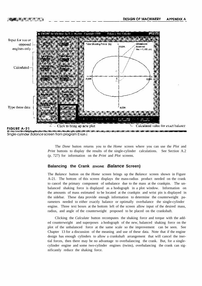
The Done button returns you to the Home screen where you can use the Plot andPrint buttons to display the results of the single-cylinder calculations. See Section A.2(p. 727) for information on the Print and Plot screens.
Balancing the Crank (ENGINE Balance Screen)
The Balance button on the Home screen brings up the Balance screen shown in FigureA-21. The bottom of this screen displays the mass-radius product needed on the crankto cancel the primary component of unbalance due to the mass at the crankpin. The un-balanced shaking force is displayed as a hodograph in a plot window. Information onthe amounts of mass estimated to be located at the crankpin and wrist pin is displayed inthe sidebar. These data provide enough information to determine the counterweight pa-rameters needed to either exactly balance or optimally overbalance the single-cylinderengine. Three text boxes at the bottom left of the screen allow input of the desired mass,radius, and angle of the counterweight proposed to be placed on the crankshaft.
Clicking the Calculate button recomputes the shaking force and torque with the add-ed counterweight and superposes a hodograph of the new, balanced shaking force on theplot of the unbalanced force at the same scale so the improvement can be seen. SeeChapter 13 for a discussion of the meaning and use of these data. Note that if the enginedesign has enough cylinders to allow a crankshaft arrangement that will cancel the iner-tial forces, then there may be no advantage to overbalancing the crank. But, for a single-cylinder engine and some two-cylinder engines (twins), overbalancing the crank can sig-nificantly reduce the shaking force.

Assembling a Multicylinder Engine (Engine Data Screen)
Once the single-cylinder configuration is satisfactorily designed and balanced, the en-gine can be assembled. Figure A-22 shows the Engine Data screen used for assembly ofa multicylinder engine. Its Help button brings up the information shown in Figure A-23,which points out that the crank phase diagram (called a Power Chart in program ENGINE)as defined in Section 14.2 (p. 644) and shown in Figures 14-8, 14-11, 14-13, 14-15,14-17, and 14-23 (pp. 646-672) should be defined and drawn manually before proceed-ing with the assembly of the engine. The assumptions and conventions used in the pro-gram to number the cylinders and banks are also stated on these screens. These are thesame conventions as defined in Section 14.7 (p. 661). The upper limit stated in item 7 ofFigure A-23 for the acceptable range of power stroke angles will be either 3600 for a two-stroke engine or 7200 (as shown) for a four-stroke engine.
The firing order, the crankshaft phase angles, and the angles at which the cylindersfire (firing angles)-all angles in cylinder order-are typed in the boxes on the right ofthe Engine Data screen based on an arrangement according to the rules in Figure A-23.Note that the program does not do any internal check on the compatibility of thesedata. It will accept any combination of phase angles, firing orders, and power strokeangles you provide. It is up to you to ensure that these data are compatible and realistic.
The program also needs the distance between cylinders which is defaulted to one.This information is used to define the Zi in equation 14.11 (p. 667). If you want to com-

pute the correct magnitude of the shaking moment, the actual cylinder spacing of yourdesign needs to be supplied in the box at the left of the screen in Figure A-22. If youonly want to compare two or more engine designs on the basis of relative shaking mo-ment, then the default value of one will suffice. The computation sums moments aboutthe first cylinder, so its moment arm is always zero. The small offset between a vee engine'sbanks, due to having two conrods per crank throw, is ignored in the moment calculation.
Charts (Pull-Down Menu)
Figure A-24 shows the Charts pull-down menu on the Home screen. Several summariesof engine information are available there. The Force Balance, Moment Balance, andTorque Balance menu selections display the results of engine balance condition calcula-tions, Le., equations 14.3a and l4.3b (p. 648) for force balance; l4.7a and l4.7b (p. 650)for moment balance; and l4.5a, l4.5b, and l4.5c (p. 650) for torque balance. (Thesecharts are also accessible from the Engine Data screen via its Balance button.)

The Power Chart selection presents the three plots shown in Figure A-25. FigureA-25a is a plot of the crankshaft phase angles over 360° for the 90° vee eight engine de-signed in Section 14.7 (p. 661). FigureA-25b shows the power stroke angles in cylinderorder over 720° for this vee eight. This is the same as the crank phase diagram shown inFigure 14-23 (p. 672) and indicates when the power pulses will occur in each cylinderduring the cycle. Figure A-25c shows the power stroke angles in firing order over 720°.This third plot rearranges the order of the cylinders on the power chart to match that of theselected firing order. If these three factors, crankshnft phnse angles, firing order, and firingangles have all been correctly chosen for compatibility, this third power chart plot will ap-pear as a staircase. The power pulses should occur in equispaced steps across the cycle ifeven firing has been achieved. Thus these power chart plots can serve as a check on the cor-rect choices of these factors. Note that the program only draws the boxes on the crank phasediagrams and power charts which represent the power strokes of each cylinder. The otherpiston strokes shown in Figures 14-8, 14-11, 14-13, 14-15, 14-17, and 14-23 (pp. 646-672)are not drawn.
Flywheel Calculations
Figure A-26 shows the Flywheel Data screen from program ENGINE. The only input tothis screen is the flywheel coefficient of fluctuation which must be between a and 1.When the Calc button is clicked, it does the same pulse-by-pulse integration of the totaltorque curve as is done in program FOURBAR. See Section 11.11 and Figure 11-16 (p.548). The areas under the pulses of the total torque curve are a measure of energy vari-ation in the cycle. The flywheel size is based on these energy variations as defined in Sec-
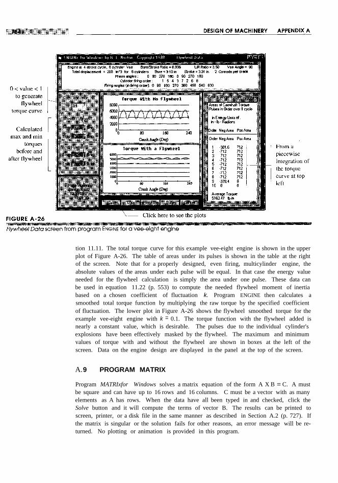
tion 11.11. The total torque curve for this example vee-eight engine is shown in the upperplot of Figure A-26. The table of areas under its pulses is shown in the table at the rightof the screen. Note that for a properly designed, even firing, multicylinder engine, theabsolute values of the areas under each pulse will be equal. In that case the energy valueneeded for the flywheel calculation is simply the area under one pulse. These data canbe used in equation 11.22 (p. 553) to compute the needed flywheel moment of inertiabased on a chosen coefficient of fluctuation k. Program ENGINE then calculates asmoothed total torque function by multiplying the raw torque by the specified coefficientof fluctuation. The lower plot in Figure A-26 shows the flywheel smoothed torque for theexample vee-eight engine with k = 0.1. The torque function with the flywheel added isnearly a constant value, which is desirable. The pulses due to the individual cylinder'sexplosions have been effectively masked by the flywheel. The maximum and minimumvalues of torque with and without the flywheel are shown in boxes at the left of thescreen. Data on the engine design are displayed in the panel at the top of the screen.
A.9 PROGRAM MATRIX
Program MATRIxfor Windows solves a matrix equation of the form A X B = C. A mustbe square and can have up to 16 rows and 16 columns. C must be a vector with as manyelements as A has rows. When the data have all been typed in and checked, click theSolve button and it will compute the terms of vector B. The results can be printed toscreen, printer, or a disk file in the same manner as described in Section A.2 (p. 727). Ifthe matrix is singular or the solution fails for other reasons, an error message will be re-turned. No plotting or animation is provided in this program.

MATERIAL PROPERTIESFor selected engineering materials. Many other alloys are available.
The following tables contain approximate values for strengths and other specificationsof a variety of engineering materials compiled from various sources. In some cases thedata are minimum recommended values and in other cases are data from a single testspecimen. These data are suitable for use in the engineering exercises contained in thistext but should not be considered as statistically valid representations of specificationsfor any particular alloy or material. The designer should consult the materials' manufac-turers for more accurate and up-to-date strength information on materials used in engi-neering applications or conduct independent tests of the selected materials to determinetheir ultimate suitability to any application.
Table No. Description
B-1 Physical Properties of Some Engineering Materials
B-2 Mechanical Properties for Some Wrought-Aluminum Alloys
B-3 Mechanical Properties for Some Carbon Steels
B-4 Mechanical Properties for Some Cast-Iron Alloys
B-5 Mechanical Properties for Some Engineering Plastics
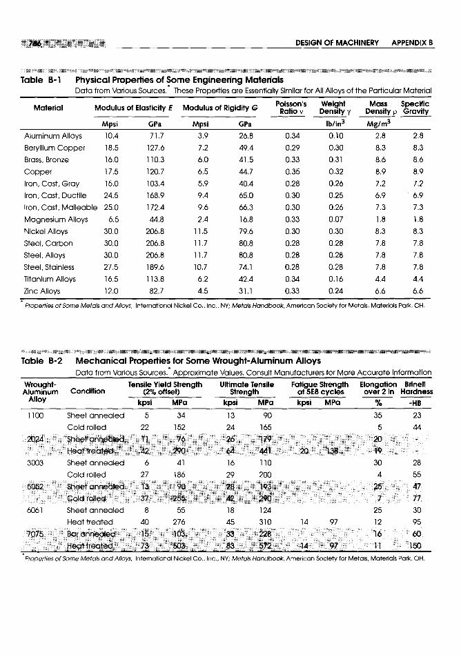

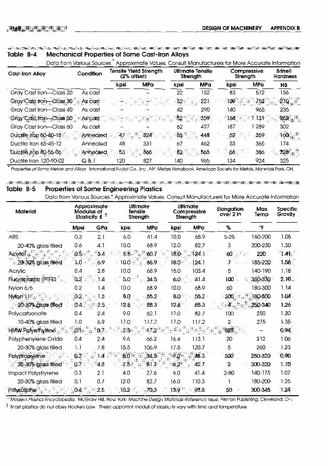


SPRING DATA
The following catalog pages of helical compression and extension spring dataprovided courtesy of Hardware Products Co., Chelsea, Massachusetts.
771


ATLAS OF GEARED FIVEBARLINKAGE COUPLER CURVESC. Zhang, R. L. Norton, T. Hammond
The following pages of coupler curve data are excerpted from the complete work.See Sections 3.6 (p. 103), 4.8 (p. 164), 6.8 (p. 278), and 7.4 (p.319) for moreinformation on the geared fivebar linkage. Use program FIVEBAR to investigateother linkage geometries.


atlas of coupler curves ball bottom dead center (BDC) 601fourbar 104, 105 and socket 25 boundarygeared fivebar 111,744 joint 25 conditions 345, 352, 378, 383
automobile bank brainstorming 10clutch 554 angle 661 brake 462suspension 107, 120, 262 engine 643 branchwheel balancer 590 of cylinders 600
axis Barker 49defect 173, 228
of rotation 495definition 173
base circleof slip cam 397, 410
brute force and ignorance
cam-follower 255, 398 440, 442, 448(BFI) 726
gearinverted slider- involute 435
building blocks 28crank 278, 314, 541 radius 396 bump steer 262
slider block 267, 269, 270 base units 17 Burmester curves 220of transmission 437 bushing 59
cam-follower 398 beam
gear teeth 436 cantilever 511 ball 122
inverted slider-crank 278, 541 double cantilever 511slider block 267, 269, 270 indeterminate 32 C
axle 262 simply supported 32bearing 55 earn 6, 24, 78, 126, 325, 345, 685
B ball 56 and follower 77, 125, 254bushing 59 automotive valve 509, 699
babbitt 635effective diameter 58 axial 349, 422
backdrive 80, 448effective length 58 barrel 349, 372flange-mount 56 contour 410
background journal 55 cylindrical 349research 9, 16, 567, 719 linear ball 56 definition 345
backhoe 7 pillow block 56 design
backlash 438, 440 ratio 58, 59 fundamental law of 356
definition 438 definition 58 desmodromic 705
balance poor, example of 59 disk 500, 686
complete 570 roller 56 duplicating machine 417
dynamic 570, 574 rolling-element 56 dynamic test fixture 415
tires 590, 591 sleeve 55 face 349
mass 571 spherical rod end 56 force-closed 704, 707
shafts 658, 676, 678 belt 6, 24, 432 form-closed 704, 705, 707
single-plane 571 flat 451 geometric generation 413
static 570, 571, 678 synchronous 451 ground 424
tires 590 timing 451 hand-dressing 414
balancer vee 433, 450 manufacturing 412
Lanchester 679 Berkof-Lowen method 580 master 416
Nakamura 679 big end (conrod) 615 materials 412
balancing 514 binary 33mechanisms 503
dynamic 577, 580, 678 link 24milled 424
linkages 580 binomialplate 349, 708
effect on input torque 585, 586 expansion 609plunge cutting 413, 414
effect on pin forces 583radial 349, 422
theorem 608, 613optimum counterweights 586
scallops 413, 414
shaking force 579, 580bisector 128 stationary 406
shaking moment 586 blank paper syndrome 8, 556 three-dimensional 350
single-cylinder engine 631 blobs 17, 18 track 704
static 573 bore/stroke ratio 634 cam·follower 40, 42, 46, 59Boston rocker 266 camoid 350

camshaft 704 Clerk 603 concave 403, 404torque 707 cycle 601 conjugate
capacitor 504, 506 engine 603 action 448carburetor 603 clockworks 5 cams 348, 702, 705
carry through 48 closed conjugates 348, 435cartesian curve 103 connecting rod 28, 600
coordinates 154 kinematic chains 28 conrod 605, 614, 617form 147 loop 64 two per crank throw 669plot 732 mechanism 28 conrodlcrank ratio 634
Cayley diagram 113, 116 closed-form solution conservation of energy 515degenerate 113 definition 174 conservative mode 686
center clutchof curvature 409 automobile 554, 623 constant
of gravity 493, 494, 531, 614 synchromesh 474 acceleration 363
global 495 coefficientof integration 688
of percussion 498, 615 of damping 503, 508velocity 385
of rotation 498, 500, 615 of fluctuation 553, 554, 623, 764 constrained 28
point 217 of friction 501 construction angle 98circle 217 cognate 113, 117 contact ratio 444
centrifugal force 514, 676 fourbar linkage 112 minimum 444
centrodes 263 geared fivebar 113 continuation methods 226fixed, moving 265 colinearity 80, 98 continuous 42noncircular gears 450 combined functions motion 385
centros 249 for cams 362, 372 continuous numerical controlchain 24 common (CNC) 413, 414
drive 432, 451 normal 255, 436, 437 convex 403silent 451 tangent 255, 435 coordinate system 24, 146, 522
change points 48 communication 16, 722 absolute 17, 146characteristic equation 690, 691 complex global 146, 191, 537, 740
Chasles'theorem 151, 247 motion 23 local 146
Chebyschev 112, 119, 120, 218 conrod 614 nonrotating 146, 522, 538, 740
chordal action 452 coupler 28, 103 rotating 146, 538, 740
cinematique 5definition 24, 149 coriolis acceleration 313, 315Whitworth slider-crank 45 correction planes 575, 678
circle number 154 cost 78arc 122 notation 154, 156
with remote center 103 plane 154coulomb friction 501, 540
point 217 component countercircle 217 orthogonal 160
balance 54
circuit compoundcouple 575
defect 173, 228 rotating eccentrics 676
definitionepicyclic train 466 shaft 474173 gear train 445, 453, 454
circuits weight 573, 585, 633, 678
of a linkage 158, 159compression crankshaft 631
ignition 605 optimum balance 586distinguishing 175 stroke 602number of 173 coupler 103, 105, 168, 718
circularcomputer aided as a physical pendulum 586
gears 265drafting 77, 105, 556 attachment points
interpolation 416engineering 77, 78 alternate 91
pitch 440manufacturing 413 curve equation 227
civil engineering 5computer graphics 97 curves 103, 104, 107, 111, 113, 128
computer programs: See programs, atlas of 105clearance 438, 440 computer degenerate 103
degree of 103

design charts 111 cycloidaldouble points 104
Denavit, J. 6, 112
shapes of 104coupler curve 267 densitydisplacement
symmetrical 107359, 362, 375 mass 493
definition 28compared 369 weight 493
output 83, 85, 89, 91dynamic force 698 derived unit
point 105, 128, 735, 749dynamic torque 708
17
crank 105, 600, 614single-dwell 382 descriptive geometry 5, 722
vibration 418 design 7, 78, 717
definition 28eccentric 58
cylinder axiomatic 15
phase diagram 644, 659, 761air and hydraulic 65 by successive analysis 77, 78
short 58spacing (IC engines) 762 case study 718
throw 641
computer aided 13
crank-conrod ratioD definition 7
608 detailed 12, 13, 14, 18
crank-rocker 48, 105 d' Alembert 5, 513, 515, 517, 571,process 3, 7, 8, 14, 20, 76, 493, 717
crank-shaper 45 617, 619qualitative 77
crank-slider dampers 511, 696ratios 634
quick-return 102 combining 504simplicity in 46
threebar 525 in parallel 505specifications 9
crankpin 617 in series 504trade-off 60, 553, 634
splayed 675 damping 502, 503, 509, 685, 689,desmodromic 348, 422, 703
crankshaft 603, 641 699determinant 213
balance weights 631 coefficient 503diametral pitch 441
mirror symmetric 659 critical 690, 691, 692Diesel cycle 605
phase angles 763 effective 504, 509differential 462
phase diagram 644 internal 512 automotive 478
creative process 10, 718 nonlinear 502center 478
definition 718 pseudo-viscous 503rear 478
creativity 7, 10, 20, 718 quadratic 502definition 477
critical extreme position (CEP) ratio 690, 695, 699limited slip 478
346, 351, 353viscous 502
Torsen 478
critical path motion (CPM) 346, DC component 609digitizing increment 419
351, 385, 386, 391, 395 decision matrix 12dimensional synthesis 78,80,
crossed dedendum 440, 44282, 132
helical gears 447circle 440
of a fourbar linkage 82
mechanism 158, 210 deferred judgment 10Dirac delta functions 356
crossover shock 422, 438, deflection 493, 501discontinuities 356
704, 706 bending 511discriminant 691
crowned pulley 451 torsional 511 displacement
crunode 104, 111 degree 103, 111, 378 carn 352, 373
cubic functiondegree of freedom 22, 27, 32, 506
definition 147
finding roots of 174definition 28
total 149
current 504distribution of 38
dissipative element 696
curvilinear translation 117spatial mechanisms 32 Dixon, A. 14
cuspvisualizing 27 DOF. See degree offreedom
on earn 404Dejonge 6 dot product 515
on coupler curve 104, 107, 111delta double
on moving centrode 267phase angle 644 crank 48
cycloidoptimum 644 dwell 130, 353
curve 104power stroke angle 654 linkage 128, 352
gear tooth 435triplet 37, 38, 42 enveloping wormset 448
geometrically generated 413deltoid 49 harmonic 375, 708

parallelogram linkage 48 eccentricity flat-four 675
rocker 48, 80, 89, 119 cam twin 674
drag link 48, 100 definition 398 radial 643
dragged crank 100 using to control pressure rotary 643
driver 60angle 401 vee 600, 643, 661
crank 534earn-follower eight 600, 661, 669, 670, 675, 763
89effect on pressure angle 401 six 661, 675
stage flat-faced 402, 411 twelve 675driving torque 538, 612 roller 398 epicyclic gear trainduplicate planar linkages 79 effective circulating power in 471
dwell 42, 60, 126, 128, 352, 423 damping 509 efficiency of 473
earn linkage 345, 433 equation solver 178, 513, 556double 698 links 40, 257 equilibrium 502, 513single 375 mass 508 equivalent
definition 125 spring 508 mass 506linkages 126 efficiency 447, 515mechanism 42, 125, 130
spring 508definition 470 system 503, 509, 685
motion 103 of a conventional gear train 470 Erdman, A. 6, 97, 188, 220dyad 83, 191, 193, 196, 205, 217 of an epicyclic train 471
definition 28 elastomers 450ergonomics 16
driver 87, 89, 91 electric motors 60, 548Euclidean geometry 82
output 100, 102, 126 electrical circuit 504Euler 5
DYNACAMprogramequivalents 156
exampleselectromechanical devices 79 identity 155
constant velocity 388 endpoint specification 351 theorem 150
force 699, 700, 705 energy Eureka! 721polynomial 382 kinetic 241 Evans, J. 5radius of curvature 406 in cam-followers 363, 372, 392 evolute 435single-dwell 374 in flywheels 549, 622torque 708, 709 in lever ratios 508 exhaust stroke 603
general information 725 in resonance 696 external
how to run 757, 764 in rotating systems 496 gearset 442
dynamic in virtual work 515, 517 load 531
analysis 18peak 370 torque 533
balancinglaw of conservation 515
devices requiring 575 method 515, 545 Fmachine 590 potential 515, 696
equilibrium 513 storage 696 face width (gears) 440force 4, 18, 144, 323, 493 elements 696
analysis 491, 521 ENGINEFerguson's paradox 466, 469
measurement 709 program 598, 609, 620, 639 film advance mechanism 105
friction 501 flywheel calculations 623 finite
models 492 engineering 14difference method 15
system 4, 514, 522 approach 14element method 15
dynamic equivalence 587 design 4, 7, 76, 126 firing
requirements for 614 costin 78 angles 763
definition 7 even 652
E human factors 16 inline engines 655
report 16 inline four 658, 660, 661
engines 60, 600vee eight 673
E-Quintet 37 vee engines 674
eccentricinline 641 order 655, 671, 763
413six-cylinder 675 652earn multicylinder 641
pattern
crank 58 opposed 643uneven 655
masses 676, 677 FIVEBARprogram

example 52 centrifugal 514, 515, 619 FOURBARprogram 81, 111, 521
cognate offourbar 120 closed 27 examples
coupler curves 112 closure 27, 348, 702 cognates 116exact straight line 120 crankpin 628, 631 coupler curve 105
how to run 725 dynamic 598 fivebar equivalent 120
fixed cam-follower 699, 700. 702, quick-return 98
centrode 263, 266 705, 708 straight-line linkages 120
pivots 90, 93, 105, 112 compared to gravitational 516 three-position synthesis 90, 209
specified 93 minimizing 362 toggle 171
flexure hinge 719 external 517, 571 two-position synthesis 198
flight simulator 726externally applied 523 how to run 725
fluctuation 553gravitational 516, 522 Fourier 5
flywheel 63, 497, 545impact 699 series 609, 648
inertia 506, 517, 557, 571, 610, free body 514, 526calculation
in program DYNACAM 708617, 629 diagram 522, 531, 619, 626, 686,
in program FOURBAR 549link 107 689
in program ENGINE 763 main pin 628 free choices 84
designingpiston sidewall 627 for function synthesis 223
for fourbar linkage 548 primary 660 in three-position
for 1C engine 622 reaction 534 synthesis 204, 205
effect 585secondary 660 in two-position
engine 622, 623shaking 544, 570, 598 synthesis 192, 193, 196
in IC engines 675cancelling 677 free vector 248, 307, 308fourbar linkage 584
materials 554 frequency
moment of inertia of 623in inline engines 646, 660
physical 554in one-cylinder engines 610, 617 forcing 695, 696
in vee engines 667 fundamental 688, 696, 702
size 763 primary 658 harmonics 688
sizing 553 secondary 658 natural 685
follower 685 spring 500, 686 and resonance 696
earn 79, 345, 435 transducer 590, 709 cam-follower 699, 700,
aligned 398 transmission 82703, 713
force-closed 686, 698 wrist pin 628, 631circular 688. 694
form-closed 702 form-closure 27, 348, 702undamped 688, 689
system 345. 685 four-stroke cycle 601, 655vs. forcing frequency 697
underdamped 696 ratio 695
flat-faced 348, 407, 423 fourbar linkage 46, 113, 531, 570 response 709
float 422acceleration 308 Freudenstein, F. 6, 157
force- or form-closed? 422 antiparalle10gram 48 friction 27, 433, 619
Jump 422, 696, 699, 700 change points 48 belts 433
mushroom 348classification of 49 force 528
roller 704cognates 116 in linkages 82
rotating 347character of 113
slipcoupler curves 104
nonlinear 502
704 torque 758
translating 347crank-rocker 40, 80 work 267
flat-faced 509 double-rocker 80, 83
roller 708 link1ess 265frisbee 248
translating or rotating? 421 mechanism 718frustration 10, 11, 720
velocity 707nine independent parameters of 224 full joint 25,29
foot-pound-second (fps) system 17 optimum straight-line 122 function
forcequick-return 98 forcing 694, 713
analysissubchain 83 generation 78, 351
dynamic 492, 698 symmetrical 108 analytical synthesis 220
kinetostatic 698, 700. 702, 705triple-rocker 48, 80 definition 79, 188
applied 523, 527table of free choices 223two-position 83

generator 78, 221, 345 gearbox 432, 455 plane 112
functional visualization 9 geared tivebar Gruebler 29
fundamental frequency 609 coupler curves 111 cri terion 38
fundamental lawmechanism 52, 164 equation 29, 32, 33, 40
of carn design 359, 698analysis 164, 319
of gearing 434, 436, 438cognate offourbar 119 H
definition 436 coupler curves 103
fuzzy logic 226, 228inversions of 53 Hachette 5program for 744
gearingHain, K. 6
G fundamental law of 434 half
definition 436 angle identities 158
gas gears 24, 434cycloid 393, 394, 395
force 605, 610, 620, 629, 652, 759 noncircular 265, 450joint 27, 33
curve 605, 610 profile-shifted 444period harmonic 393
pressure 610, 759 gearset 434, 448Hall, A. S. 6, 97, 98, 119
curve 603, 605, 610 angle of approach 437 Hammond, T. 111
torque 610, 613, 652, 759 angle of recess 437 harmonic 375
gate 105 arc of action 437 number 675
Gauss-Jordan elimination 200 changing center distance 438 harmonics 609, 648, 688
gear contact ratio 444, 446 Hartenberg, R. 6, 112
antibacklash 439 external 435 helical motion 25
base pitch 444 highest point of single-tooth helix angle 25, 447, 448bevel 449 contact 444
spiral 449 internal 435, 442higher pair 6, 25, 27
straight 449 length of action 436, 444Hitchcock chair 266
blank 449 pressure angle 437 hob (gear) 442
helical 447 genetic algorithms 226 hodograph 732
herringbone 447 GenevaHoeken linkage 120, 122
hypoid 450 mechanism 42 homogeneous 688
idler 453, 744rack 449
wheel 42 ODE 688
ratio 112, 164, 506, 744global mass center 580 solution 689
set 119, 265goal statement 9,567 homotopy methods 226
shaper 442 graphical hood hinge 79
spur 447dimensional synthesis 78 Hrones and Nelson atlas 104
teeth 435compare to analytical 196 human factors engineering 15, 21
full-depth 442 tools needed for 83, 89 hunting 439
minimum number 442 position analysis 145 hydraulicunequal addendum 444 Grashof 47, 144 cylinder 77
tooth action 432 condition 46, 47, 49, 89
train 432, 452 geared fivebar 53motor 60, 65
compound 454 crank-rocker 120hyperboloids 450
design algorithm 458 double-rocker 170hypoid gears 450
earliest known reference 432 fivebar 119epicyclic 461, 462, 465, 475 linkage 60 Ierror in center distance 438 special case 48irrational ratio 461 gravitational idea generation 10reverted 456, 474simple 452 constant 17, 18 ideation 9, 11, 14, 720
worm 448system 17 and invention 9
wormset 448gravity 323 identification of need 8
ground identity matrix 200
definition 28 imaginary axis 154pivots 95
4

imbalance 590 isomer 38, 746 kinetostatics 492, 521, 698, 706inch-pound-second (ips) 17 invalid 38 Kinsyn 97inclined plane 5 number of valid isomers 38 KISS 15incubation 11, 720 iteration 8, 11, 13, 77, 82, 84, Koster 503, 696, 698, 699, 713indexers 372 386, 493, 556 Kota, S. 109indexing 125 J Kutzbach 29
table 371indices of merit 261 Linduction system 602 jacobian 176, 177
inductor 504, 505 jerk 324, 374 Lagrange 5inertia angular 325, 326 Lanchester balancer 679
balance 658earn 352
L'Ecole Polytechnic 5difference 327vee engine 661, 674finite 696, 698 length of action 436, 444
force 513, 514, 571, 619, 643, 652linear 327 Levai
torque 513, 517, 620, 649jitter 128 12 basic epicyclic trains 463
inertial reference frame 146joint 6, 25 lever 5
infinity of solutions 196, 217earn-follower 56 ratio 506, 511
inflection points 383, 406 cantilevered 57 limit stops 107initial conditions 688 force-closed 27 Lincages 78, 97, 220inner ear 322 force index 169, 555 lineinput torque 548, 585 form-closed 27 contact 25instant centers 249 multiple 30, 33 of action 437
earn-follower 254, 400 one-freedom 25 of centers 105fourbar linkage 250, 263, 718 order 27 lineargenerate centrodes 265 slider 25 acceleration 300, 323permanent 249, 250 sliding 250 actuator 65, 66slider-crank 252 straddle mounted 58 algebra 199using in linkage design 261 two-freedom 25 ball bearings 56
intake stroke 602 joystick 25 Geneva mechanism 44interference 442 graph 249intermittent motion 42, 385 K interpolation 414, 419
internal combustion jerk 325
engine 538, 598, 639 Kant 5 motion 65velocity 241invention 7, 10 Kaufman, R. 97, 188
Kennedy, Alexander 6 link 6, 23, 24, 38inverse dynamics 492, 521, 698 dogbone 587inversion Kennedy's rule 249, 250
output 144definition 44 Kimball, B. 726 ratio 105, 111for three-position kinematic shrinkage
synthesis 93, 95, 97 applications 6 complete 40, 42in ideation 11 chain 27 partial 40of slider-crank 102 class of 47, 53, 54 linkage 78
force analysis 541 definition 27 advantages 59, 60position solution 162 inversion of 47 assemblability 54
inversions pair 6, 25 basic building blocks 24, 53distinct 45 structure 30, 32 compliant 263of fourbar linkage 47 synthesis 521 design 24of sixbar linkages 44 kinematics 3, 4, 5, 491, 685, disadvantages 60
involute 435, 438, 442, 448 699, 709 inline 586definition 435 definition 3 linkless 266teeth 438 history of 5, 20 non-quick-return 98
kinetics 3, 5, 491 rotatability 46

self-locking 81, 91 mass-spring model 686 single DOF 512sixbar 167
Stephenson's 167masses statically equivalent 616
Watt's 167combining 506 value of 617
synthesis 78, 80, 112massless rod 498, 571 modified
torque 82, 90 materials 635 sine 367, 372, 394, 418, 698
transformation 33, 40, 345 Mathcad 178, 556, 400 trapezoid 367, 369, 418
linkages 6, 24 Matlab 400 module 441
connected in parallel 53 matrix modulus
connected in series 53 augmented 200, 205, 213of elasticity 509
versus cams 59 coefficient 205 of rupture 511
linkless fourbar linkage 267 inverse 200 moment
load solution 199, 513 primary 658
lines 61 solver 199, 513 secondary 658, 660
torque 61 MATRIXprogram shaking 570, 598, 677
load sharing 444 examplein inline engines 650, 652
locomotive 48force analysis 529, 531, 534 in vee engines 667
Loerch 188, 211linkage synthesis 209 momentum 492, 603
log roller 5force analysis 513 Monge, Gaspard 5how to use 201 motion
losses 516, 696 May, Rollo 718 complex
lower pair 6,25 mechanical definition 149lubricant 25 advantage 260, 261, 435 generation 89, 189
lubrication 55, 60, 424, 603 analog computer 78 analytical synthesis 193hydrodynamic 55 circuit 504 definition 79problems 56 efficiency 260
three-position 89, 91seals for 55 engineering 5
two-position 85
lumped function generator 78intermittent 65
mass 576,616 system 504parallel 117
model 508, 617, 685 mechanism 4, 5, 27, 32, 144simple harmonic 357, 358
parameter 506, 511 crank-shaper 103straight line 77
definition 4, 27motor 28, 60, 517
M double-dwell 130AC 60
forces in 491closed loop 64
machine 4, 5, 27, 144non-quick-return 98
compound-wound 61, 62
definitionoptical adjusting 263
DC 604, 27
design 3, 5, 18, 59, 76, 325planar 79
permanent magnet (PM) 61
machineryquick-return 97
speed controlled 63Whitworth 103
gearmotor 60, 64
rotating 497open loop 65
mandrel 590microcomputer 13, 78 permanent magnet 61
mass 4, 18, 492, 500, 614, 686,Milton, J. 432 series-wound 62
696, 699mirror symmetric 659, 675 serv0 60
balance 572mks system 18 shunt-wound 62
density 493 mobility 28. See also degree of speed torque characteristic 548
effective 508, 509, 699, 708 freedom stepper 60, 65, 79
equivalent 614 model 13, 206, 495, 503synchronous 63
lumped 509, 615 cardboard 13, 81, 85universal 60
moment 493, 494, 580 dynamic 498., movie camera 105
moment of dynamically equivalent 614 moving
inertia 495, 522, 550, 585, 614 finite element 600 centro de 265, 266
point 492, 498, 571 lumped mass 617 pivots 90, 95, 128
mass-radius product 573, 578, lumped parameter 686 multiple solutions 15
591, 633 simplified 492

N oversquare engine 634 piston 324, 539, 600, 614, 617overturning moment 402 acceleration 606, 610, 619
Nakamura balancer 679engine 45
natural frequency 679, 688, 709 P position 606
circular 688pump 45, 538, 601, 639
damped 688, 691 pairs 25velocity 606
undamped 688, 691 higher 25pitch
Nelson, G. L. 104 lower 25circle 435, 438, 440
Newton-Raphson paradoxescurve 397, 404, 406
method 168, 174, 327 Ferguson's 468diameters 435, 438
chaotic behavior of 175 Gruebler's 37diametral 441
in equation solvers 178 parallelpoint 435, 436
Newton's axis theorem 497, 557planet gear 462
equation 17, 686 connectionsplatform rocker 266
laws 323, 491, 521, 571 dampers 504 polar
method 174,521 springs 504 coordinates 154
second law 3linkage planes 79 form 147
third law 527motion 117 plot 660, 732
no-load speeds 64 parallelogram linkage 48, 49 poles 249
node 24, 28, 38 particular solution 688, 694 polodes 265
noise, vibration, and harshness path 79 polynomial 708
(NVH) 679 generation 79 3-4-5 378, 381, 382, 698
non-Grashof 47definition 79 4-5-6-7 381, 382, 418
double-rocker 170precision points 189 function 356, 378
number synthesis 33with coupler curve 103, 105, design rule 383
107, 112numerical control (NC) 413 with prescribed timing 79, 220
position 144, 147, 241
nut 25 pawlabsolute 149
driving 44analysis 151, 152
0difference 148
locking 44 equation 147, 243Peaucellier 122 of any point on a link 168
objective function 224 performance specifications 9, 14, relative 148
octoid 449 567, 719 vector 147, 153
offset (in slider-crank) 159 phase angle pounds force (lbf) 18
oil bath 424 crankshaft 641, 763 pounds mass (Ibm) 17
opengeared fivebar 111, 164, 744 power 61, 259, 504, 516, 653, 706
kinematic chain 28optimum 641 chart 761, 763
mechanism 158, 210sign convention 644 equation 517
operator 154physical pendulum 586 stroke 603, 655, 659
orderpiecewise continuous function 359 angles 653, 655, 763
defect 228piezoelectric
to weight ratio 601
of joints 27accelerometer 709 practical
of links 33force transducer 590 considerations 554, 556, 713
of polynomial 378 pin precision
orthogonal 160 double shear 58 points 189, 196
oscillation - earn-follower 696forces 610, 623 position 189, 191, 201
Otto cycle 601crankpin 626 preload
overbalanced crankmain pin 628 earn-follower spring 699
633 wrist pin 626overdamped system 691 joint 25, 55
preloaded structure 32
overlays 77 single shear 58pressure angle
overshoot of response 692 pinion 434, 449earn-follower 396
flat-faced 437

force analysis 708 dynamics 745 pureroller 397. 398 input data 744 harmonic 553, 652, 689
of gearsets 437 phase angle defined 744 rolling 27, 104, 498, 570primary component FOURBAR 735 joint 27
of shaking force 609 balancing in 740 rotation 24, 85, 241, 614, 617of shaking moment 652 centrodes 739 slide 27
cognates 743 translation 24, 312, 498, 614, 617prime input data 735 pushrod 509circle 397, 708 synthesis 743radius 396, 405 general information 725 Qprincipal axes 23 home screen 728
principle how to run them 735of d' A1embert 513 linkage quasi-static 513of transmissibility 258 angle steps 736 quaternary link 24, 33
problem animation 738 quickdefinition 719 autoscaling 739 forward 98unstructured 8 calculation errors 738 return 98, 102, 105
problem sets calculation in 736 mechanism 45dynamics 740 sixbar 100Chapter 2 67 Grashof condition 738Chapter 3 132 one position 736 RChapter 4 178 time steps 737Chapter 5 232 trace on/off 739Chapter 6 281 MATRIX 764 rack 449Chapter 7 327 opening a file 729 and pinion 449Chapter 8 425 operation 727, 743 steering 449Chapter 9 479 plotting data 731 radiusChapter 10 518 cartesian plots 732 of curvature 396Chapter 11 557 polar plots 732 flat follower 407Chapter 12 592 printing from 730 roller follower 403, 405Chapter 13 635 quitting 734 of gyration 498, 500Chapter 14 682 running 728 prime circle 700Chapter 15 714 saving data 729 ratchet 6
production 13 SIXBAR 745 and pawl 44programs, computer animation 748 wheel 44
coordinate systems in 732, 740 dynamics 748 ratiocopying to clipboard 729 input data 746
506SLIDER 749 gear
creating new files 729 lever 508animation 751disclaimer on liability 726calculation 750 reference frame 28
DYNACAM 751dynamics 751 relativecontinuity check 754input data 749 acceleration. See acceleration:drawing the cam 755
follower dynamics 756 support 735 relativeinput data 751 units 729 velocity. See velocity: relativepolynomial functions 753 user actions possible 728 report, technical 16sizing the cam 754 projects resistor 504
ENGINE 757 Chapter 3 140 resonance 696charts 762 Chapter 8 429 earn-followercrank balancing 760 Chapter 11 567 force-closed 696flywheel calculations 763 Chapter 13 638 form-closed 703multi cylinder 761 Chapter 14 683 resonate 695single cylinder 758 prototypes 13, 511examples in 729 response
prototyping 12 complete 695FIVEBAR 743and testing 13 damped 689animation 745
coupler point 744 pulleys 450 forced 695

steady state 695 rotation 23 mechanism 124. 126
transient 688, 692, 695 definition 149 enveloping wormset 448
undamped 686 pure 24 gearset 453
Reuleaux, Franz 6, 25, 28 balance in 570 sixbar
classification of mechanisms 27 rotational drag-link quick-return 100
reverted DOF 25 linkage 113
compound train 456 freedom 27 mechanism 126
gear train design 456 kinetic energy 601 Watts linkage 89
revolvability 54 rotopole 85 SIXBARprogram 725
definition 54 roughness, surface 419 differences from FOURBAR 746
right angle drives 449example 53
rigid body 23,24 Sdouble-dwell 130, 352
acceleration 308quick-return 102
motion 149 s v a j diagrams 352single-dwell 128three-position synthesis 93, 211
ring gear 462 polynomials 378 two-position synthesis 89
rise-dwell-fall-dwell cam 346, 351 Sanders 327 skew axis 23
rise-fall cam 346, 351 Sandor, G. N. 6, 97, 188 slider block 40, 539
rise-fall-dwell cam 346, 351, 374 scalar magnitude 256 slider-crank 40, 45, 60, 103, 250,
Roberts scaling 13 538, 541
-Chebyschev theorem 112 Scotch yoke 40,44 analysis
diagram 113 screw 6acceleration 311
straight -line linkage 120 joint 25 Fourier 605
Roberts, Richard 120 secondinstant centers 252
Roberts, Samuel 112, 120 harmonic 609position solution 159
robot 28,77vector loop 159
moment inverted 161, 316, 541rocker
of area 511 acceleration 315arm 509, 511 of mass 495 linkage
definition 28 secondary component dynamic model 617infinitely long 40 of shaking force 609 in lC engines 598
output 83 of shaking moment 652 multicy linde r 639
rockingselection 12 offset 161
chair 266 series connectionsone-cylinder 600
couple 575 dampers 504 nonoffset 605
roll-slide joint 25,27 springs 504 offset
roller 348 servodefinition 159
chain 451 mechanisms 439 sliding
follower 348, 405, 423, 500, 686 motor 64, 79 contact 6
chrome plated 423 valve 65 joints 33
crowned 423 shaftslip 104
in valve trains 423 encoder 590 component 269, 270, 314
materials 423 hollow 462 velocity 313
slip 422 sheave 450slop 439
rolling shock 324slugs 17, 18
centrodes 450 SI systemsolenoid 28, 66, 77
17cones 449 solids modelling 556
contact 6 simple harmonic motion 394
cylinders 433, 435 simultaneous equationsolution methods 512
root finding 327solution 199 Soni, A. 117
rotatability 46,53dynamic forces 512, 522 space width (gears) 438, 440
definition 53 single spatial
of geared fivebar linkage 53 cylinder engine 600 linkage 107
of N-bar linkages 53 dwell 130, 374, 382 mechanisms 27, 79

specified fixed pivots 93, 95, 211 sweet spot 498 toggle 80, 81, 265, 737
spreadsheet 513 synchromesh 448, 474 angle 172
spring clutch 474 linkage 81
compression 510, 511 transmission 474 position 80, 91, 113, 189, 19(
constant 55, 500, 509, 511, 686, synonyms 11 calculating location 170
700, 704 synthesis 76, 77, 80, 83in rock crusher 261
definition 501 algorithm 78tolerance 414
effective 506, 508, 698, 704 analytical 78, 82(human) of acceleration 323
free length 699 compare to graphical 196 tooth thickness 438, 440helical coil 699 elastic energy method 229 toothed belts 451physical 698, 704 equation 224 top dead center (TDC) 601preload 700 equation methods 227 torque 585
springs 107, 505 optimization methods 227 about the mass center 495as links 54 optimized 224 applied 523combining 505 precision 224 camshaft 706, 708in parallel 506 precision point methods 226
selective precision synthesis 228 converter 475in series 505 using genetic algorithms 229 driving 517
sprocket 451 definition 8 dynamic 708
standard form equation 220, 222 four-position external 517
static analytical 220 flywheel-smoothed 623
equivalence 617 graphical 97 gas 613
friction 501 graphical flywheel smoothing 622stationary configuration 80 tools needed for 83 in four-cylinder inline engine
steady state 688 of mechanisms 3, 18, 22 655, 660
qualitative 76, 77, 78, 84 in one-cylinder engine 610Stephenson's quantitative 78, 97 in vee engines 669
chain 38, 40 inertia 610sixbar 45, 53, 167, 746, 747
three position flywheel smoothing 622analytical 201, 205, 208
stepper motor 60, 65, 69 graphical 89 in four-cylinder inline engine
stiction 501 motion 201 658, 660
stiffness 493, 696 specified fixed pivots 211, 214 in inline engines 649
44, 372 two position 83in one-cylinder engine 621
stops in vee engines 668straight-line
analytical 197 in virtu61 work 517linkage 5, 77
graphical 89 input 5~5, 706, 707optimum 122 type 78 oscillations in 707
mechanisms 120 T ratio 260, 435approximate 122 shaking 544, 610exact 120 in fourbar linkage 586
strain gages 709 tabular method 465 in multicylinder engines 652strength 493 tackle 6 in one-cylinder engines 620
stresses 4, 144, 323, 493 tappet 509 source 523, 528, 534, 557
structural ternary link 24, 33, 34 total 660, 673, 763
building block 37 testing 12, 13engine 622
variation 548subchain 38 thermodynamics 598, 605 torque-speed relation 61
structure 30, 32 three-freedom joint 25preloaded 32 threebar crank-slide 525
torque-time
Suh, N. P. 15diagram 551
through variable 504 function 622sun gear 462 time ratio 98, 100, 102 Towfigh, K. 263, 717, 718superposition 512, 513, 610, 623 timing diagram 353 trade-offs 78, 126, 374, 703surface contact 25 Ting, K. L. 53 train ratio 453suspension system 262 TKSolver 178, 327, 400, 556

transfer unobtainium 614, 698 Wport 603 unstructured problem 8theorem 497Watt, James 5transient 688 V Watt'sanalysis 737
chain 38, 53translating valve 509 linkage 746follower 347 earn 422, 434 sixbar 40, 45, 83, 167, 746slider 100 float 699 straight-line fourbar 120translation 23,24 spring 509 wear 25curvilinear 117, 149 valves 345 weather systems 315definition 149vector wedge 5rectilinear 149, 348
angle oftranslational DOF 25 weight 17definition 156factor 12transmission 435, 448, 601 free 248, 307, 308
well pump 45automatic 468 loop 191automotive 474 wheel 6veecomponent 269, 270, 314 angle 643, 661, 674 and axle 5crashbox 477 belt 450 Whitworth quick-return 45, 103Ford model T 476 velocity 144, 241 Willis, Robert 5synchromesh 474
absolute 242, 247, 248 windshield wiper linkage 49transmission angle 257, 258, analysis Wood, George A. Jr. 717261, 503, 554 algebraic 271 work 28, 515definition 81, 169 geared fivebar 278 Working Model 77, 81, 105, 725differences in cognates 113 graphical 244, 246448extreme values 169 inverted slider-crank 270 worm
limited application 169 sliding joint 268 set 448minimum 82 using instant centers 256 wheel 448optimal 102 angular 241, 270, 277, 315 wrapping connectors 6poor 196 earn 352 wrist pin 615, 617quick-return linkage 100 constant 120 writing engineering reports 21
trapezoidal definition 241acceleration 363 difference 243, 247, 248, 272, 302 Yrule 552 equation 243
triple-rocker 48, 170 of point on link 279Young's modulus 509, 511of slip 267, 277, 315truss 38
of transmission 278twobar chain 83, 100 ratio 435, 442, 450 Ztwo-dimensional space 23 of involute gears 438two-freedom joint 25 relati ve 243, 247, 267, 272, 501 zero velocity 104two-plane balance 574 vibration Zhang, C. 111, 744two-stroke in cam-
cycle 601, 603, 653 followers 396, 503, 694, 704engine 654 in engines 652
type synthesis 77, 131 in linkages 544residual 698 "
U virtual work 515, 517, 545equation 517 i·,1
undercutting 404, 407, 442 ViseGrip 261underdamped 692, 693 visualization 721, 722undersquare engine 634 voltage 504unit vectors 154units systems 16