development ii seminar documentation
TRANSCRIPT

Development II seminar DocumentationRelease 0.1
Jonathan Conning
Oct 04, 2018

Contents
1 Development Microeconomics with Jupyter Notebooks 31.1 Economics with Jupyter Notebooks . . . . . . . . . . . . . . . . . . . . . . . . . . . . . . . . . . . 31.2 Lucas (1990) “Why Doesn’t Capital Flow from Rich to Poor Countries?” . . . . . . . . . . . . . . . 81.3 Edgeworth Box: Efficiency in production allocation . . . . . . . . . . . . . . . . . . . . . . . . . . 161.4 The Specific Factors or Ricardo-Viner Model . . . . . . . . . . . . . . . . . . . . . . . . . . . . . . 241.5 Migration, urban-bias and the informal sector . . . . . . . . . . . . . . . . . . . . . . . . . . . . . . 371.6 Coase, Property rights and the ‘Coase Theorem’ . . . . . . . . . . . . . . . . . . . . . . . . . . . . 441.7 Farm Household Models . . . . . . . . . . . . . . . . . . . . . . . . . . . . . . . . . . . . . . . . . 551.8 Testing for Separation in Household models . . . . . . . . . . . . . . . . . . . . . . . . . . . . . . . 661.9 Equilibrium Size Distribution of Farms . . . . . . . . . . . . . . . . . . . . . . . . . . . . . . . . . 691.10 Causes and consequences of insecure Property Rights to land . . . . . . . . . . . . . . . . . . . . . 801.11 Consumer Choice and Intertemporal Choice . . . . . . . . . . . . . . . . . . . . . . . . . . . . . . 841.12 Quasi-hyperbolic discounting and commitment savings . . . . . . . . . . . . . . . . . . . . . . . . . 941.13 Notes on Incentive Contracts and Corruption . . . . . . . . . . . . . . . . . . . . . . . . . . . . . . 1021.14 Research Discontinuity Designs (in R) . . . . . . . . . . . . . . . . . . . . . . . . . . . . . . . . . 1111.15 Data APIs and pandas operations . . . . . . . . . . . . . . . . . . . . . . . . . . . . . . . . . . . . 1221.16 Stata and R in a jupyter notebook . . . . . . . . . . . . . . . . . . . . . . . . . . . . . . . . . . . . 1281.17 Jupyter running an R kernel . . . . . . . . . . . . . . . . . . . . . . . . . . . . . . . . . . . . . . . 1281.18 Jupyter with a Stata Kernel . . . . . . . . . . . . . . . . . . . . . . . . . . . . . . . . . . . . . . . . 1291.19 Python and Stata combined in the same notebook . . . . . . . . . . . . . . . . . . . . . . . . . . . . 129
i

ii

Development II seminar Documentation, Release 0.1
Lecture Notes and materials for The Graduate Center’s Economics 842 taught by Jonathan Conning
• Reading list (links to weekly reading assignments and slides)
• Syllabus (course details and longer bibliography)
These reading and lecture notes on development microeconomics are written mostly as interactive jupyter notebookswhich are kept at this github repository.
• https://github.com/jhconning/Dev-II
See below for different ways to access and interact with this content.
Contents 1

Development II seminar Documentation, Release 0.1
2 Contents

CHAPTER 1
Development Microeconomics with Jupyter Notebooks
List of notebooks:
1.1 Economics with Jupyter Notebooks
• Jupyter Notebook is “a web application that allows you to create and share documents that contain live code,equations, visualizations and explanatory text. Uses include: data cleaning and transformation, numerical sim-ulation, statistical modeling, machine learning and much more.”
• Open-source, browser-based
• Evolved from ipython notebook to leverage huge scientific python ecosystem.
• Now a ‘language agnostic’ platform so that you can use any of 50+ other kernels including MATLAB, Octave,Stata, Julia, etc.
• Open-source, fast evolving, large community: Widely used in academic and scientific computing community.
• Ties projects together: Code, data, documentation, output and analysis all in one place.
• Encourages reproducible science:
• Easy workflow from exploratory analysis to publish.
• Works well with github and other open-source sharing tools.
1.1.1 Ways to view and run jupyter notebooks
Jupyter server for interactive computing Run on a local machine or cloud server to modify code and results on thefly.
• On your computer:
– Jupyter notebook on your local machine. I recommend using Anaconda to install Jupyter and scientificpython. A good instalation guide here
3
Development II seminar Documentation, Release 0.1
– nteract. A good one-click install solution for running notebooks. Provides you with standalone programthat installs scientific python and runs jupyter notebooks (not quite full functionality).
• Jupyter notebooks are big in the data science space. Lots of free cloud server solutions are emerging:
– Microsoft Azure notebooks: Setup a free account for cloud hosted jupyter notebooks.
– Google Colaboratory: Run notebooks stored on your google drive.
– Cocalc: jupyter notebooks, SageMath and other cloud hosted services.
– Try Jupyter: another cloud server, but you can’t save work at all.
Static rendering for presentations and publishing.
• Jupyter notebooks can be rendered in different ways for example as a styled HTML slideshow or page or as aPDF book by using tools and services such as github, nbconvert, Sphinx and Read the Docs.
• This very notebook is:
– hosted on the Dev-II repository on github where it is rendered in simple HTML (though underlying formatis json).
– viewable in HTML or as javascript slideshow via nbviewer. To then see in slideshow mode click on‘present’ icon on top right.
– Tied together with other documents via Sphinx to create a website on readthedocs
– Also viewable as a PDF book on readthedocs
1.1.2 A simple jupyter notebook example:
We can combine text, math, code and graph outputs in one place. Let’s study a simple economics question:
Are average incomes per capita converging?
Neoclassical growth theory:
• Solow-growth model with Cobb-Douglas technology 𝑓(𝑘) = 𝑘𝛼.
• Technology, saving rate 𝑠, capital depreciation rate 𝛿, population growth rate 𝑛 and technological change rate 𝑔assumed same across countries.
• Steady-state capital per worker to which countries are converging:
𝑘* = (𝑔/𝑠)1
𝛼−1
• Transitional dynamics:
��(𝑡) = 𝑠𝑘(𝑡)𝑡 − (𝑛 + 𝑔 + 𝛿)𝑘(𝑡)
• Diminishing returns to the accumulated factor 𝑘 implies convergence:
• Lower initial capital stock implies lower initial per-capita GDP.
• Country that starts with lower capital stock and GDP per capita ‘catches up’ by growing faster.
4 Chapter 1. Development Microeconomics with Jupyter Notebooks
Development II seminar Documentation, Release 0.1
Convergence plots
Did countries with low levels of income per capita in 1960 grow faster?
I found a dataset from World Penn Tables on this website (original data source here).
Let us import useful python libraries for data handling and plots and load the dataset into a pandas dataframe:
In [1]: import matplotlib.pyplot as plt%matplotlib inlineimport pandas as pdimport seaborn as snsfrom ipywidgets import interact
df = pd.read_stata(".\data\country.dta")
(in the future we will follow best practice and place library imports at the top of our notebooks).
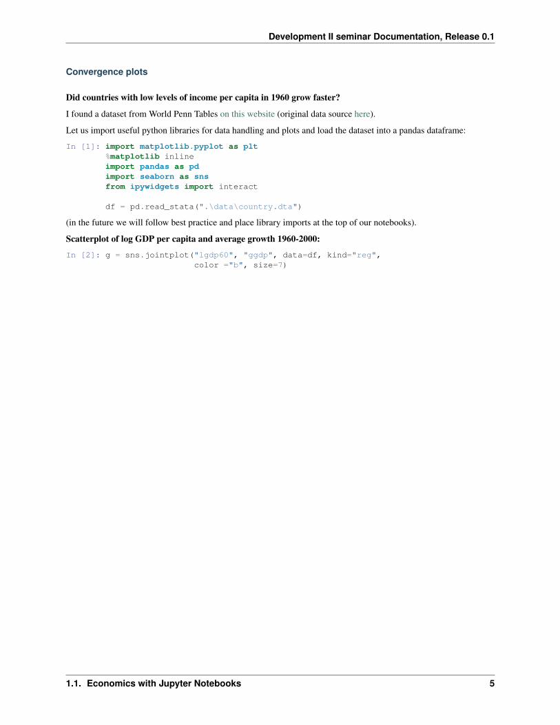
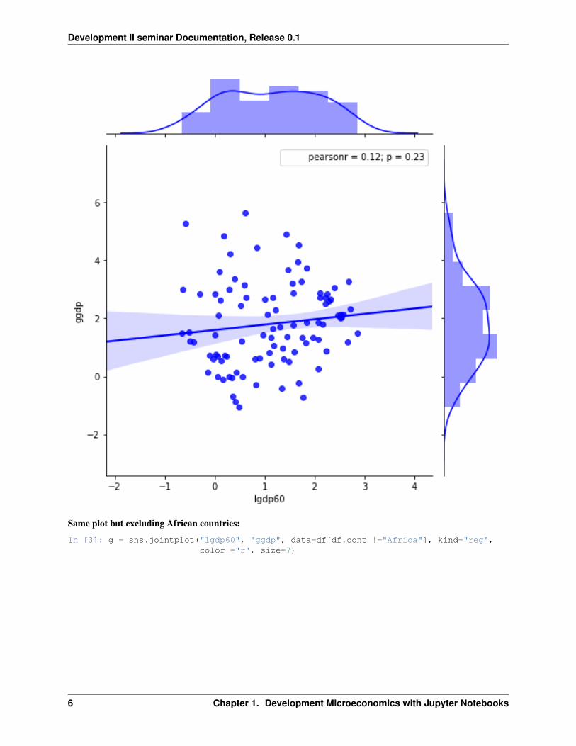
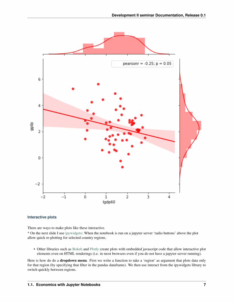
Scatterplot of log GDP per capita and average growth 1960-2000:
In [2]: g = sns.jointplot("lgdp60", "ggdp", data=df, kind="reg",color ="b", size=7)
1.1. Economics with Jupyter Notebooks 5
Development II seminar Documentation, Release 0.1
Same plot but excluding African countries:
In [3]: g = sns.jointplot("lgdp60", "ggdp", data=df[df.cont !="Africa"], kind="reg",color ="r", size=7)
6 Chapter 1. Development Microeconomics with Jupyter Notebooks
Development II seminar Documentation, Release 0.1
Interactive plots
There are ways to make plots like these interactive.* On the next slide I use ipywidgets: When the notebook is run on a jupyter server ‘radio buttons’ above the plotallow quick re-plotting for selected country regions.
• Other libraries such as Bokeh and Plotly create plots with embedded javascript code that allow interactive plotelements even on HTML renderings (i.e. in most browsers even if you do not have a jupyter server running).
Here is how do do a dropdown menu. First we write a function to take a ‘region’ as argument that plots data onlyfor that region (by specifying that filter in the pandas dataframe). We then use interact from the ipywidgets library toswitch quickly between regions.
1.1. Economics with Jupyter Notebooks 7
Development II seminar Documentation, Release 0.1
You’ll only see this as truly interactive on a live notebook, not in a static HTML rendering of the same notebook.
In [4]: def jplot(region):sns.jointplot("lgdp60", "ggdp", data=df[df.cont == region],
kind="reg", color ="g", size=7)plt.show();
In [5]: interact(jplot, region=list(df.cont.unique()))
Out[5]: <function __main__.jplot>
1.1.3 More on jupyter notebooks and scientific python
• An excellent introduction to Jupyter notebooks and scientific python for economists written by John Stachurskiis at this link:
http://quant-econ.net/py/learning_python.html
1.2 Lucas (1990) “Why Doesn’t Capital Flow from Rich to Poor Coun-tries?”
Summary and analytical notes on the paper:
Lucas, Robert E. (1990) “Why Doesn’t Capital Flow from Rich to Poor Countries?” American Economic Review:92-96.
Note: To change or interact with the code and figures in this notebook first run the code section below the ‘CodeSection’ below. Then run any code cells above.
1.2.1 Neoclassical trade, migration and growth model predictions:
• the convergence of factor prices and incomes per-capita over time (Factor Price Equalization Theorem)
• via substitute mechanisms: factor movement, trade in products, and/or capital accumulation (e.g. Solow).
• rests on assumptions about technology and market competition
– in particular: diminishing returns to the accumulated factor capital (i.e. 𝐹𝐾𝐾 < 0 ).
Simplest model
Assume two countries with same aggregate production function, where 𝑋 is capital stock and 𝐿 is labor force:
𝑌 = 𝐴𝑋𝛽𝐿1−𝛽
in intensive or per-capita form:
𝑦 = 𝐴𝑥𝛽
where
𝑦 =𝑌
𝐿and 𝑥 =
𝑋
𝐿
Marginal Product of Capital is:
𝑟 = 𝐴𝛽𝑥𝛽−1
8 Chapter 1. Development Microeconomics with Jupyter Notebooks
Development II seminar Documentation, Release 0.1
Marginal Product of Capital (MPK) as a function of income per capita:
𝑟 = 𝛽𝐴1𝛽 𝑦
𝛽−1𝛽
or
𝑟 = 𝐴𝛽( 𝑦
𝐴
) 𝛽−1𝛽
Steps:
𝑦 = 𝐴𝑥𝛽
𝑠𝑜
𝑥 =( 𝑦
𝐴
) 1𝛽
substitute this into 𝑟 = 𝐴𝛽𝑥𝛽−1
The puzzle
• Let capital share 𝛽 = 0.4 (average of USA and India)
• Assume first that 𝐴 is the same in both countries
• In 1988 income per capita in USA was 15 times higher than USA:𝑦𝑈𝑆
𝑦𝐼𝑁= 15
• this implies MPK in India would have to be:
𝑟𝐼𝑁𝑟𝑈𝑆
=
[𝑦𝑈𝑆
𝑦𝐼𝑁
] 1−𝛽𝛽
= 58.1
times higher in India! Implausibly large.
What differences in capital per worker account for this large a gap?
As $x =({ 𝑦𝐴}
)ˆ𝑡ℎ𝑖𝑠multiple of the amount of capital per worker compared to India:
So if in India the capital-labor ratio is 1 in the USA it must be 871.4 !
• With such huge differences in returns, capital would surely RUSH from USA to India quickly lower the gap inreturns and incomes.
• Evidently it does not. So what’s wrong with the model? Lucas walks through 4 alternate hyptotheses.
Some plots
In [9]: print('Return to capital in India relative to USA : {:5.1f}'.format(r(y_IN, A)/r(y_US, A)))
Return to capital in India relative to USA : 58.1
The ratio of capital stock per worker in the USA compared to India that is implied by this difference in incomes percapita is even more unbelievable:
In [10]: print('Capital per worker in USA relative to India : {:5.1f}'.format(kap(y_US, A)/kap(y_IN, A)))
Capital per worker in USA relative to India : 871.4
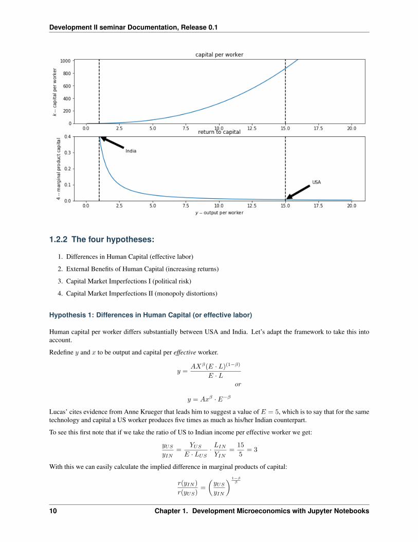
In [11]: lucasplot()
1.2. Lucas (1990) “Why Doesn’t Capital Flow from Rich to Poor Countries?” 9
Development II seminar Documentation, Release 0.1
1.2.2 The four hypotheses:
1. Differences in Human Capital (effective labor)
2. External Benefits of Human Capital (increasing returns)
3. Capital Market Imperfections I (political risk)
4. Capital Market Imperfections II (monopoly distortions)
Hypothesis 1: Differences in Human Capital (or effective labor)
Human capital per worker differs substantially between USA and India. Let’s adapt the framework to take this intoaccount.
Redefine 𝑦 and 𝑥 to be output and capital per effective worker.
𝑦 =𝐴𝑋𝛽(𝐸 · 𝐿)(1−𝛽)
𝐸 · 𝐿𝑜𝑟
𝑦 = 𝐴𝑥𝛽 · 𝐸−𝛽
Lucas’ cites evidence from Anne Krueger that leads him to suggest a value of 𝐸 = 5, which is to say that for the sametechnology and capital a US worker produces five times as much as his/her Indian counterpart.
To see this first note that if we take the ratio of US to Indian income per effective worker we get:
𝑦𝑈𝑆
𝑦𝐼𝑁=
𝑌𝑈𝑆
𝐸 · 𝐿𝑈𝑆· 𝐿𝐼𝑁
𝑌𝐼𝑁=
15
5= 3
With this we can easily calculate the implied difference in marginal products of capital:
𝑟(𝑦𝐼𝑁 )
𝑟(𝑦𝑈𝑆)=
(𝑦𝑈𝑆
𝑦𝐼𝑁
) 1−𝛽𝛽
10 Chapter 1. Development Microeconomics with Jupyter Notebooks
Development II seminar Documentation, Release 0.1
= 31.5 = 5.2
So this lowers the factor of proportionality from 58 to 5. As Lucas puts it: “This is a substantial revision but it leavesthe original paradox very much alive: a factor of five differnce in rates of return is tstill large enough to lead one toexpect capital flows much larger than anything we observe (p. 93).”
Hypothesis 2: External Benefits to Human Capital
We’ve assumed thus far that the total factor productivity parameter 𝐴 is the same across countries. This is unlikely.An easy way to resolve the paradox is to simply solve for the level of A_{US}/A_{IN} that makes he gap dissappear.
In this section Luca isn’t quite doing that but he is in effect letting the values of A differ between the two countries.He motivates this with a stripped down version of his own Lucas (1988) paper on external economies, a model wherehuman capital plays a role and where there is a positive external effect in human-capital accumulation in that heassumes that the marginal product of one’s human capital is augmented by the average level of human capital in theeconomy. In this paper he doesn’t work out this model in full but uses the story to rewrite the production function as:
𝑦 = 𝐴ℎ𝛾𝑥𝛽
and he then gives us some ‘guestimates’ as to the differences in human capital per worker in each country. As it turnsout this is in effect equivalent to sticking to the original model and just assuming that
𝐴𝑈𝑆
𝐴𝐼𝑁= 5
A country with a higher level of 𝐴 will have everywhere higher return on capital. After a little math the adjusted rationow becomes
𝑟(𝑦𝐼𝑁 )
𝑟(𝑦𝑈𝑆)=
(𝑦𝑈𝑆
𝑦𝐼𝑁
) 1−𝛽𝛽
=31.5
5= 1.04
This would seem to almost resolve the paradox but Lucas in fact dismisses it as not entirely realistic. It assumes forexample that knowledge spillovers across borders are zero.
### Hypothesis 3: Capital Market Imperfections I (political risk)
I haven’t written this up yet. . .
### Hypothesis 4: monopoly power distortions to capital market
This is the least often mentioned but possibly the most interesting of Lucas’ hypotheses. The hypothesis is that localelites (or ‘an imperial power’) are able to collude to control the entry of capital into India to drive up captial rentsand drive down real wages in such a way that increase firm profits. Implictly the story is that local elites control theorganization of production and hence firm profits.
While at first it might seem far-fetched to believe a story like this in modern times (less far-fetched in the time of theEast India Company) there is plenty of evidence that capital inflows into India and other developing countries werehistoricallycontrolled in part to protect the rents of local elites. Rajan and Zingales’ (2013) book Saving Capitalismfrom the Capitalists is full of examples of local elites lobbying government bureaucrats to establish market power.
The elite is assumed to have access to international capital markets where they can borrow capital at the rate $ 𝜌$
If the elite ran the country as a monopoly they would choose the capital-labor ratio (by varying how much capitalenters the country) to maximize profits per capita:
𝑓(𝑥) − [𝑓(𝑥) − 𝑥𝑓 ′(𝑥)] − 𝑟𝑥
1.2. Lucas (1990) “Why Doesn’t Capital Flow from Rich to Poor Countries?” 11
Development II seminar Documentation, Release 0.1
Here (by Euler’s Theorem) 𝑓(𝑥) − 𝑥𝑓 ′(𝑥) is the wage.
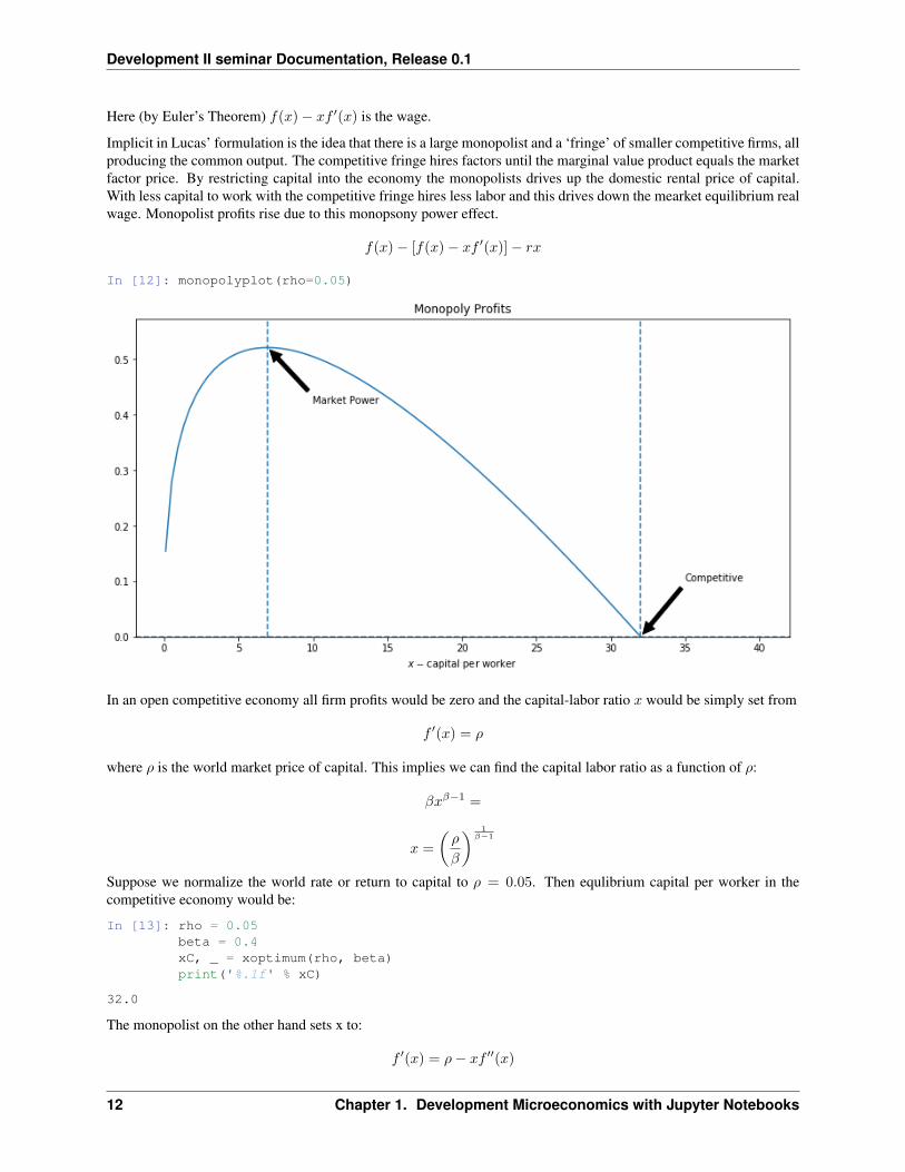
Implicit in Lucas’ formulation is the idea that there is a large monopolist and a ‘fringe’ of smaller competitive firms, allproducing the common output. The competitive fringe hires factors until the marginal value product equals the marketfactor price. By restricting capital into the economy the monopolists drives up the domestic rental price of capital.With less capital to work with the competitive fringe hires less labor and this drives down the mearket equilibrium realwage. Monopolist profits rise due to this monopsony power effect.
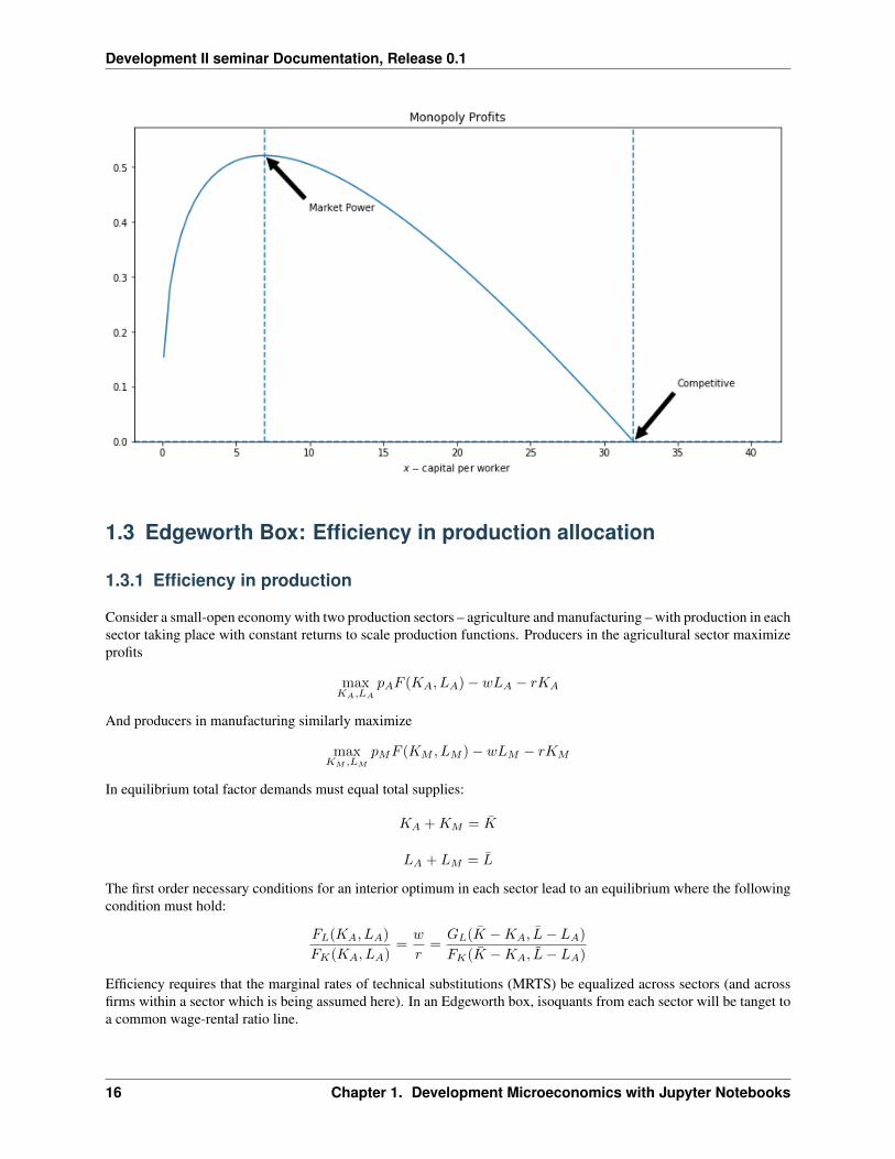
𝑓(𝑥) − [𝑓(𝑥) − 𝑥𝑓 ′(𝑥)] − 𝑟𝑥
In [12]: monopolyplot(rho=0.05)
In an open competitive economy all firm profits would be zero and the capital-labor ratio 𝑥 would be simply set from
𝑓 ′(𝑥) = 𝜌
where 𝜌 is the world market price of capital. This implies we can find the capital labor ratio as a function of 𝜌:
𝛽𝑥𝛽−1 =
𝑥 =
(𝜌
𝛽
) 1𝛽−1
Suppose we normalize the world rate or return to capital to 𝜌 = 0.05. Then equlibrium capital per worker in thecompetitive economy would be:
In [13]: rho = 0.05beta = 0.4xC, _ = xoptimum(rho, beta)print('%.1f' % xC)
32.0
The monopolist on the other hand sets x to:
𝑓 ′(𝑥) = 𝜌− 𝑥𝑓 ′′(𝑥)
12 Chapter 1. Development Microeconomics with Jupyter Notebooks
Development II seminar Documentation, Release 0.1
Note that 𝑓 ′′(𝑥) can be written:
𝑓 ′′(𝑥) = (𝛽 − 1)𝑓 ′(𝑥)
𝑥
which allows us to simplify the monopoly FOC to:
𝑓 ′(𝑥) =𝜌
𝛽
Given our assumed value of beta, this means a monopolist might maintain the rate of return on capital 1/𝛽 timeshigher than the international market rate 𝜌, and resists capital inflows that might push this rate down.
Solving for 𝑥 in this monopolized market gives:
𝑥 =
(𝜌
𝛽2
) 1𝛽−1
In [14]: _ , xM = xoptimum(rho, beta)print('Capital per worker in the market-power distorted equilibrium: {:2.1f}'.format(xM))print(' {:.0%} of the competitive level'.format(xM/xC))
Capital per worker in the market-power distorted equilibrium: 6.922% of the competitive level
Indian income per capita will be only
In [15]: print("{:5.0f} percent".format(100*f(xM)/f(xC)))
54 percent
as high as in a competitive market without barriers to capital inflows.
This is an inefficient outcome but the elites who capture the profits/rents do pretty well. They earn
In [16]: print('profits = {:5.2f} or {:.0%} of total output'.format(profit(xM, rho), profit(xM,rho)/f(xM)))
profits = 0.52 or 24% of total output
1.2.3 Extensions
Lucas does not cite their work but models of this sort were explored by trade economists in the 1980s (e.g. Feenstra(1980).
In a model described later, Conning (2006) explores similar factor market power distortions in a model with heteroge-nous agents to make predictions about the size distribution of firms within each sector.
Solving for maxima and roots numerically
This was an easy model to solve analytically, but let’s solve it numerically to illustrate the use of the root solving(fsolve function from scipy optimize library) and minimization techniques (brentq from the same library). See thecode section below first.
Let’s setup first order condition functions to find the x that sets them to zero.
For the competitive case: $f’(x) - 𝜌$𝐹𝑜𝑟𝑡ℎ𝑒𝑚𝑜𝑛𝑜𝑝𝑜𝑙𝑦𝑐𝑎𝑠𝑒 : 𝑓 ′(𝑥) − 𝜌− 𝑥𝑓 ′′(𝑥)
In [17]: def cfoc(x):return mpx(x) - rho
def mfoc(x):return mpx(x) - rho + (beta-1)*mpx(x)
1.2. Lucas (1990) “Why Doesn’t Capital Flow from Rich to Poor Countries?” 13
Development II seminar Documentation, Release 0.1
and solve for the root:
In [18]: from scipy.optimize import fsolve, brentq, minimizexC = fsolve(cfoc, 20)[0]xC
Out[18]: 32.0
Same as the analytical solution of course.
Now let’s find the 𝑥 that maximizes monopoly profits (we need to provide a guess value):
In [19]: xM = fsolve(mfoc, 5)[0]xM
Out[19]: 6.9489090984826332
We could have instead directly maximized profits (minimized negative profits) with an optimization routine:
In [20]: def negprofit(x):return - profit(x, rho)
res = minimize(negprofit, 5, method='Nelder-Mead')res.x[0]
Out[20]: 6.94891357421875
## Code Section
To unclutter the notebook above much of the code has been moved to this section. To re-create or modify any contentgo to the ‘Cell’ menu above run all code cells below by choosing ‘Run All Below’. Then ‘Run all Above’ to recreateall output above (or go to the top and step through each code cell manually).
In [1]: %matplotlib inlineimport numpy as npimport matplotlib.pylab as plt
In [2]: A = 1rho = 0.05beta = 0.4y_US = 15y_IN = 1
def f(x):return x**beta
def mpx(x):return beta*x**(beta-1)
def r(y, A):return beta * (A**(1-beta)) * y**((beta-1)/beta)
def kap(y, A):return (y/A)**(1/beta)
In [3]: def xoptimum(rho, beta):xC = (rho/beta)**(1/(beta-1))xM = (rho/beta**2)**(1/(beta-1))return xC, xM
In [4]: def lucasplot():y = np.linspace(0.1,20,100)plt.figure(figsize=(12, 6))plt.subplot(2,1,1)plt.plot(y,kap(y, A))
14 Chapter 1. Development Microeconomics with Jupyter Notebooks
Development II seminar Documentation, Release 0.1
plt.ylabel("$k$ -- capital per worker")plt.ylim(0,kap(y_US +1, A))plt.axvline(y_IN,color='k',ls='dashed')plt.axvline(y_US,color='k',ls='dashed')plt.title("capital per worker")
plt.subplot(2,1,2)plt.plot(y,r(y,A))plt.xlabel("$y$ -- output per worker")plt.ylabel("$4$ -- marginal product capital")plt.title("return to capital")plt.ylim(0,r(y_IN,A))plt.axvline(y_IN,color='k',ls='dashed')plt.axvline(y_US,color='k',ls='dashed')plt.annotate('India', xy=(y_IN, r(y_IN,A)), xytext=(y_IN +2, r(y_IN,A)*0.75),
arrowprops=dict(facecolor='black', shrink=0.05),)plt.annotate('USA', xy=(y_US, r(y_US,A)), xytext=(y_US +2, r(y_US,A)+0.1),
arrowprops=dict(facecolor='black', shrink=0.05),);
In [5]: def profit(x, rho):return f(x) -(f(x) -mpx(x)*x) - rho*x
In [6]: x = np.linspace(0.1,40,100)
def monopolyplot(rho):prf = profit(x, rho)xC, xM = xoptimum(rho, beta)fig, ax = plt.subplots(1, 1, figsize=(12, 6))plt.plot(x,prf)plt.ylim(0,max(prf)*1.1)plt.title('Monopoly Profits')plt.axvline(xC,ls='dashed')plt.axvline(xM,ls='dashed')plt.axhline(0,ls='dashed')plt.xlabel("$x$ -- capital per worker")plt.annotate('Competitive', xy=(xC, 0), xytext=(xC+3, 0.1),
arrowprops=dict(facecolor='black', shrink=0.05),)plt.annotate('Market Power', xy=(xM, profit(xM,rho)), xytext=(xM+3, profit(xM,rho)-0.1),
arrowprops=dict(facecolor='black', shrink=0.05),)plt.show()
In [7]: monopolyplot(0.05)
1.2. Lucas (1990) “Why Doesn’t Capital Flow from Rich to Poor Countries?” 15
Development II seminar Documentation, Release 0.1
1.3 Edgeworth Box: Efficiency in production allocation
1.3.1 Efficiency in production
Consider a small-open economy with two production sectors – agriculture and manufacturing – with production in eachsector taking place with constant returns to scale production functions. Producers in the agricultural sector maximizeprofits
max𝐾𝐴,𝐿𝐴
𝑝𝐴𝐹 (𝐾𝐴, 𝐿𝐴) − 𝑤𝐿𝐴 − 𝑟𝐾𝐴
And producers in manufacturing similarly maximize
max𝐾𝑀 ,𝐿𝑀
𝑝𝑀𝐹 (𝐾𝑀 , 𝐿𝑀 ) − 𝑤𝐿𝑀 − 𝑟𝐾𝑀
In equilibrium total factor demands must equal total supplies:
𝐾𝐴 + 𝐾𝑀 = ��
𝐿𝐴 + 𝐿𝑀 = ��
The first order necessary conditions for an interior optimum in each sector lead to an equilibrium where the followingcondition must hold:
𝐹𝐿(𝐾𝐴, 𝐿𝐴)
𝐹𝐾(𝐾𝐴, 𝐿𝐴)=
𝑤
𝑟=
𝐺𝐿(�� −𝐾𝐴, ��− 𝐿𝐴)
𝐹𝐾(�� −𝐾𝐴, ��− 𝐿𝐴)
Efficiency requires that the marginal rates of technical substitutions (MRTS) be equalized across sectors (and acrossfirms within a sector which is being assumed here). In an Edgeworth box, isoquants from each sector will be tanget toa common wage-rental ratio line.
16 Chapter 1. Development Microeconomics with Jupyter Notebooks
Development II seminar Documentation, Release 0.1
If we assume Cobb-Douglas forms 𝐹 (𝐾,𝐿) = 𝐾𝛼𝐿1−𝛼 and 𝐺(𝐾,𝐿) = 𝐾𝛽𝐿1−𝛽 the efficiency condition can beused to find a closed form solution for 𝐾𝐴 in terms of 𝐿𝐴:
(1 − 𝛼)
𝛼
𝐾𝐴
𝐿𝐴=
𝑤
𝑟=
(1 − 𝛽)
𝛽
�� −𝐾𝐴
��− 𝐿𝐴
Rearranging the expression above we can get a closed-form expression for the efficiency locus 𝐾𝐴(𝐿𝐴):
𝐾𝐴(𝐿𝐴) =𝐿𝐴 · ��
𝛽(1−𝛼)𝛼(1−𝛽) (��− 𝐿𝐴) + 𝐿𝐴
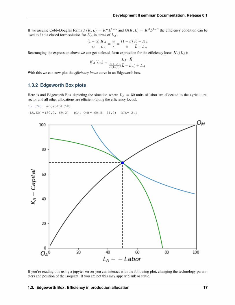
With this we can now plot the efficiency locus curve in an Edgeworth box.
1.3.2 Edgeworth Box plots
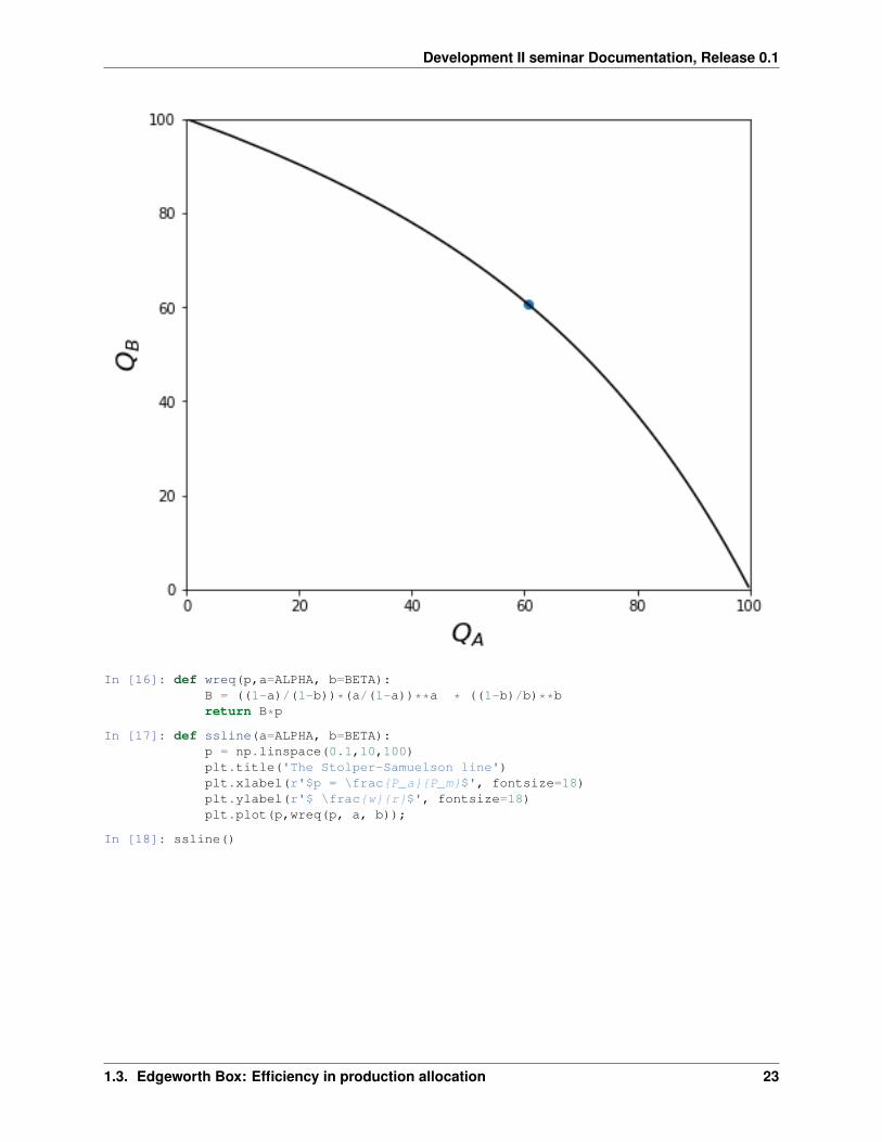
Here is and Edgeworth Box depicting the situation where 𝐿𝐴 = 50 units of labor are allocated to the agriculturalsector and all other allocations are efficient (along the efficiency locus).
In [76]: edgeplot(50)
(LA,KA)=(50.0, 69.2) (QA, QM)=(60.8, 41.2) RTS= 2.1
If you’re reading this using a jupyter server you can interact with the following plot, changing the technology param-eters and position of the isoquant. If you are not this may appear blank or static.
1.3. Edgeworth Box: Efficiency in production allocation 17
Development II seminar Documentation, Release 0.1
In [75]: LA = 50interact(edgeplot, LA=(10, LBAR-10,1),
Kbar=fixed(KBAR), Lbar=fixed(LBAR),zalpha=(0.1,0.9,0.1),beta=(0.1,0.9,0.1));
interactive(children=(IntSlider(value=50, description='LA', max=90, min=10), FloatSlider(value=0.6, description='alpha', max=0.9, min=0.1), FloatSlider(value=0.4, description='beta', max=0.9, min=0.1), Output()), _dom_classes=('widget-interact',))
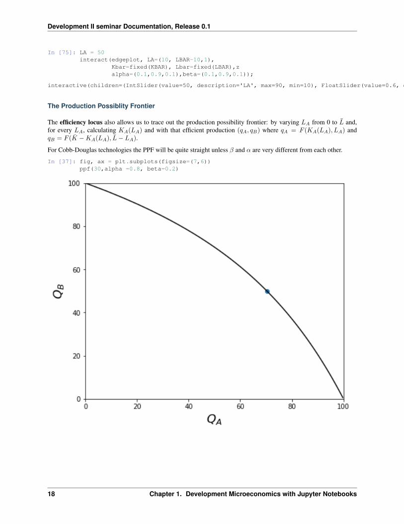
The Production Possiblity Frontier
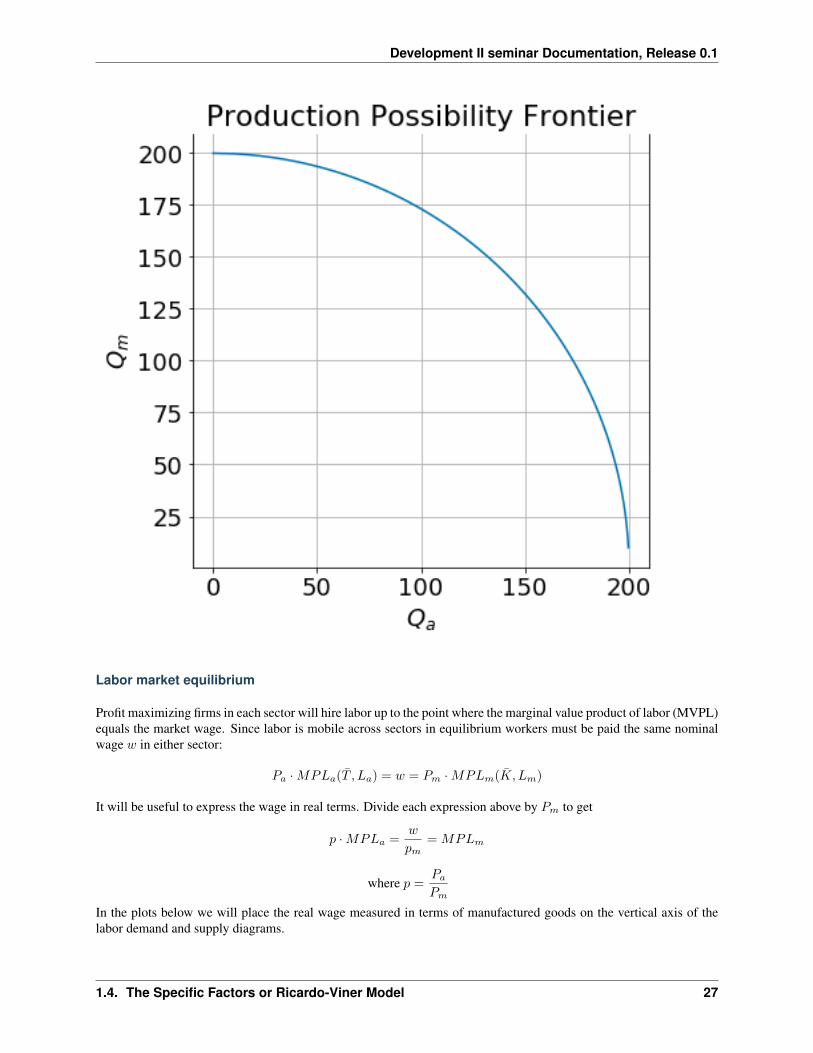
The efficiency locus also allows us to trace out the production possibility frontier: by varying 𝐿𝐴 from 0 to �� and,for every 𝐿𝐴, calculating 𝐾𝐴(𝐿𝐴) and with that efficient production (𝑞𝐴, 𝑞𝐵) where 𝑞𝐴 = 𝐹 (𝐾𝐴(𝐿𝐴), 𝐿𝐴) and𝑞𝐵 = 𝐹 (�� −𝐾𝐴(𝐿𝐴), ��− 𝐿𝐴).
For Cobb-Douglas technologies the PPF will be quite straight unless 𝛽 and 𝛼 are very different from each other.
In [37]: fig, ax = plt.subplots(figsize=(7,6))ppf(30,alpha =0.8, beta=0.2)
18 Chapter 1. Development Microeconomics with Jupyter Notebooks
Development II seminar Documentation, Release 0.1
1.3.3 Efficient resource allocation and comparative advantage in a small openeconomy
We have a production possibility frontier which also tells us the opportunity cost of producing different amounts ofgood 𝐴 in terms of how much of good B (via its slope or the Rate of Product Transformation (RPT) 𝑀𝐶𝐴
𝑀𝐶𝐵). This is
given by the slope of the PPF. The bowed out shape of the PPF tells us that the opportunity cost of producing eithergood is rising in its quantity.
How much of each good will the economy produce? If this is a competitive small open economy then product priceswill be given by world prices. Each firm maximizes profits which leads every firm in the A sector to increase outputuntil 𝑀𝐶𝑋(𝑞𝑎) = 𝑃𝐴 and similarly in the B sector so that in equlibrium we must have
𝑀𝐶𝐴
𝑀𝐶𝐵=
𝑃𝐴
𝑃𝐵
and the economy will produce where the slope of the PPF exactly equals the world relative price. This is where nationalincome valued at world prices is maximized, and the country is producing according to comparative advantage.
Consumers take this income as given and maximize utility. If we make heroic assumptions about preferences (prefer-ences are identical and homothetic) then we can represent consumer preferences on the same diagram and we wouldhave consumers choosing a consumption basket somewhere along the consumption possibliity frontier given by theworld price line passing thorugh the production point.
If the economy is instead assumed to be closed then product prices must be calculated alongside the resource allocation.The PPF itself becomes the economy’s budget constraint and we find an optimum (and equlibrium autarky domesticprices) where the community indifference curve is tangent to the PPF.
As previously noted, given our linear homogenous production technology, profit maximization in agriculture will leadfirms to choose inputs to satisfy (1−𝛼)
𝛼𝐾𝐴
𝐿𝐴= 𝑤
𝑟 . This implies a relationship between the optimal production techniqueor capital-labor intensity 𝐾𝐴
𝐿𝐴in agriculture and the factor price ratio 𝑤
𝑟 :
𝐾𝐴
𝐿𝐴=
𝛼
1 − 𝛼
𝑤
𝑟
and similarly in manufacturing
𝐾𝑀
𝐿𝑀=
𝛽
1 − 𝛽
𝑤
𝑟
From the first order conditions we also have:
𝑃𝐴𝐹𝐿(𝐾𝐴, 𝐿𝐴) = 𝑤 = 𝑃𝑀𝐺𝐿(𝐾𝑀 , 𝐿𝑀 )
Note this condition states that competition has driven firms to price at marginal cost in each industry or 𝑃𝐴 = 𝑀𝐶𝐴 =𝑤 1
𝐹𝐿and 𝑃𝑀 = 𝑀𝐶𝑀 = 𝑤 1
𝐺𝐿which in turn implies that at a market equilibrium optimum
𝑃𝐴
𝑃𝑀=
𝐺𝐿(𝐾𝑀 , 𝐿𝑀 )
𝐹𝐿(𝐾𝐴, 𝐿𝐴)
This states that the world price line with slope (negative) 𝑃𝐴
𝑃𝑀will be tangent to the production possibility frontier
which as a slope (negative) 𝑀𝐶𝐴
𝑀𝐶𝑀= 𝑃𝐴
𝑃𝑀which can also be written as 𝐺𝐿
𝐹𝐿or equivalently 𝐺𝐾
𝐹𝐾. The competitive
market leads producers to move resources across sectors to maximize the value of GDP at world prices.
With the Cobb Douglas technology we can write:
𝐹𝐿 = (1 − 𝛼)
[𝐾𝐴
𝐿𝐴
]𝛼
𝐺𝐿 = (1 − 𝛽)
[𝐾𝑀
𝐿𝑀
]𝛽1.3. Edgeworth Box: Efficiency in production allocation 19
Development II seminar Documentation, Release 0.1
Using these expressions and the earlier expression relating 𝐾𝐴
𝐿𝐴and 𝐾𝑀
𝐿𝑀to 𝑤
𝑟 we have:
𝑃𝐴
𝑃𝑀=
1 − 𝛼
1 − 𝛽
[(1−𝛽)
𝛽𝑤𝑟
]𝛽[(1−𝛼)
𝛼𝑤𝑟
]𝛼or
𝑃𝐴
𝑃𝑀= Γ
[𝑤𝑟
]𝛽−𝛼
𝑤ℎ𝑒𝑟𝑒
Γ =1 − 𝛼
1 − 𝛽
(𝛼
1 − 𝛼
)𝛼 (1 − 𝛽
𝛽
)𝛽
Solving for 𝑤𝑟 as a function of the world prices we find an expression for the ‘Stolper-Samuelson’ (SS) line:
𝑤
𝑟=
1
Γ
[𝑃𝐴
𝑃𝑀
] 1𝛽−𝛼
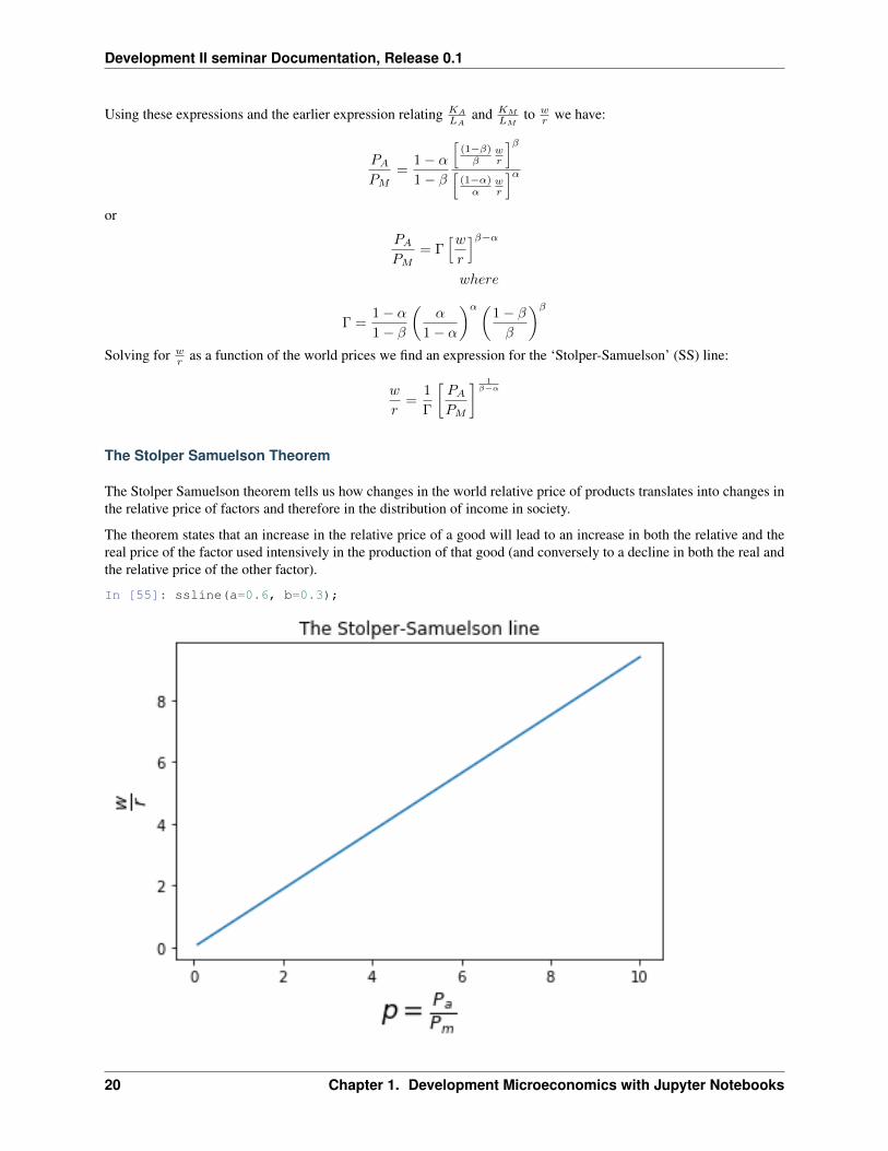
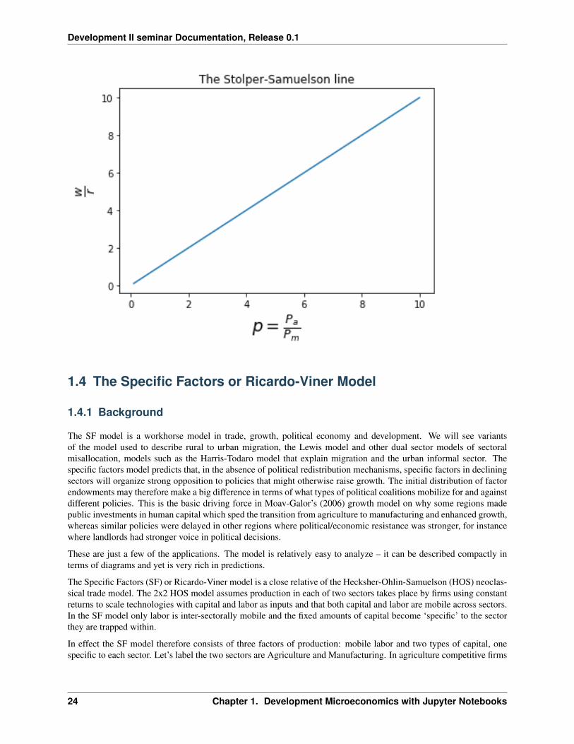
The Stolper Samuelson Theorem
The Stolper Samuelson theorem tells us how changes in the world relative price of products translates into changes inthe relative price of factors and therefore in the distribution of income in society.
The theorem states that an increase in the relative price of a good will lead to an increase in both the relative and thereal price of the factor used intensively in the production of that good (and conversely to a decline in both the real andthe relative price of the other factor).
In [55]: ssline(a=0.6, b=0.3);
20 Chapter 1. Development Microeconomics with Jupyter Notebooks
Development II seminar Documentation, Release 0.1
This relationship can be seen from the formula. If agriculture were more labor intensive than manufacturing, so 𝛼 < 𝛽,then an increase in the relative price of agricultural goods creates an incipient excess demand for labor and an excesssupply of capital (as firms try to expand production in the now more profitable labor-intensive agricultural sector andcut back production in the now relatively less profitable and capital-intensive manufacturing sector). Equilibrium willonly be restored if the equilibrium wage-rental ratio falls which in turn leads firms in both sectors to adopt morecapital-intensive techniques. With more capital per worker in each sector output per worker and hence real wages perworker 𝑤
𝑃𝑎and 𝑤
𝑃𝑚increase.
To be completed
• Code to solve for unique HOS equilibrium as a function of world relative price 𝑃𝐴
𝑃𝑀
• Interactive plot with 𝑃𝐴
𝑃𝑀slider that plots equilibrium in Edgeworth box and PPF
1.3.4 Code section
To keep the presentation tidy I’ve put the code that is used in the notebook above at the end of the notebook. Run allcode below this cell first. Then return and run all code above.
In [10]: %matplotlib inlineimport matplotlib.pyplot as pltimport numpy as npfrom ipywidgets import interact, fixed
In [11]: ALPHA = 0.6 # capital share in agricultureBETA = 0.4 #
KBAR = 100LBAR = 100
p = 1 # =Pa/Pm relative price of ag goods
def F(K,L,alpha=ALPHA):"""Agriculture Production function"""return (K**alpha)*(L**(1-alpha))
def G(K,L,beta=BETA):"""Manufacturing Production function"""return (K**beta)*(L**(1-beta))
def budgetc(c1, p1, p2, I):return (I/p2)-(p1/p2)*c1
def isoq(L, Q, mu):return (Q/(L**(1-mu)))**(1/mu)
In [12]: def edgeworth(L, Kbar=KBAR, Lbar=LBAR,alpha=ALPHA, beta=BETA):"""efficiency locus: """a = (1-alpha)/alphab = (1-beta)/betareturn b*L*Kbar/(a*(Lbar-L)+b*L)
In [13]: def edgeplot(LA, Kbar=KBAR, Lbar=LBAR,alpha=ALPHA,beta=BETA):"""Draw an edgeworth box
arguments:LA -- labor allocated to ag, from which calculate QA(Ka(La),La)
1.3. Edgeworth Box: Efficiency in production allocation 21
Development II seminar Documentation, Release 0.1
"""KA = edgeworth(LA, Kbar, Lbar,alpha, beta)RTS = (alpha/(1-alpha))*(KA/LA)QA = F(KA,LA,alpha)QM = G(Kbar-KA,Lbar-LA,beta)print("(LA,KA)=({:4.1f}, {:4.1f}) (QA, QM)=({:4.1f}, {:4.1f}) RTS={:4.1f}"
.format(LA,KA,QA,QM,RTS))La = np.arange(1,Lbar)fig, ax = plt.subplots(figsize=(7,6))ax.set_xlim(0, Lbar)ax.set_ylim(0, Kbar)ax.plot(La, edgeworth(La,Kbar,Lbar,alpha,beta),'k-')#ax.plot(La, La,'k--')ax.plot(La, isoq(La, QA, alpha))ax.plot(La, Kbar-isoq(Lbar-La, QM, beta),'g-')ax.plot(LA, KA,'ob')ax.vlines(LA,0,KA, linestyles="dashed")ax.hlines(KA,0,LA, linestyles="dashed")ax.text(-6,-6,r'$O_A$',fontsize=16)ax.text(Lbar,Kbar,r'$O_M$',fontsize=16)ax.set_xlabel(r'$L_A -- Labor$', fontsize=16)ax.set_ylabel('$K_A - Capital$', fontsize=16)#plt.show()
In [14]: def ppf(LA,Kbar=KBAR, Lbar=LBAR,alpha=ALPHA,beta=BETA):"""Draw a production possibility frontier
arguments:LA -- labor allocated to ag, from which calculate QA(Ka(La),La)"""KA = edgeworth(LA, Kbar, Lbar,alpha, beta)RTS = (alpha/(1-alpha))*(KA/LA)QA = F( KA,LA,alpha)QM = G(Kbar-KA,Lbar-LA,beta)ax.scatter(QA,QM)La = np.arange(0,Lbar)Ka = edgeworth(La, Kbar, Lbar,alpha, beta)Qa = F(Ka,La,alpha)Qm = G(Kbar-Ka,Lbar-La,beta)ax.set_xlim(0, Lbar)ax.set_ylim(0, Kbar)ax.plot(Qa, Qm,'k-')ax.set_xlabel(r'$Q_A$',fontsize=18)ax.set_ylabel(r'$Q_B$',fontsize=18)plt.show()
It’s interesting to note that for Cobb-Douglas technologies you really need quite a difference in capital-intensitiesbetween the two technologies in order to get much curvature to the production function.
In [15]: fig, ax = plt.subplots(figsize=(7,6))ppf(20,alpha =0.8, beta=0.2)
22 Chapter 1. Development Microeconomics with Jupyter Notebooks
Development II seminar Documentation, Release 0.1
In [16]: def wreq(p,a=ALPHA, b=BETA):B = ((1-a)/(1-b))*(a/(1-a))**a * ((1-b)/b)**breturn B*p
In [17]: def ssline(a=ALPHA, b=BETA):p = np.linspace(0.1,10,100)plt.title('The Stolper-Samuelson line')plt.xlabel(r'$p = \frac{P_a}{P_m}$', fontsize=18)plt.ylabel(r'$ \frac{w}{r}$', fontsize=18)plt.plot(p,wreq(p, a, b));
In [18]: ssline()
1.3. Edgeworth Box: Efficiency in production allocation 23
Development II seminar Documentation, Release 0.1
1.4 The Specific Factors or Ricardo-Viner Model
1.4.1 Background
The SF model is a workhorse model in trade, growth, political economy and development. We will see variantsof the model used to describe rural to urban migration, the Lewis model and other dual sector models of sectoralmisallocation, models such as the Harris-Todaro model that explain migration and the urban informal sector. Thespecific factors model predicts that, in the absence of political redistribution mechanisms, specific factors in decliningsectors will organize strong opposition to policies that might otherwise raise growth. The initial distribution of factorendowments may therefore make a big difference in terms of what types of political coalitions mobilize for and againstdifferent policies. This is the basic driving force in Moav-Galor’s (2006) growth model on why some regions madepublic investments in human capital which sped the transition from agriculture to manufacturing and enhanced growth,whereas similar policies were delayed in other regions where political/economic resistance was stronger, for instancewhere landlords had stronger voice in political decisions.
These are just a few of the applications. The model is relatively easy to analyze – it can be described compactly interms of diagrams and yet is very rich in predictions.
The Specific Factors (SF) or Ricardo-Viner model is a close relative of the Hecksher-Ohlin-Samuelson (HOS) neoclas-sical trade model. The 2x2 HOS model assumes production in each of two sectors takes place by firms using constantreturns to scale technologies with capital and labor as inputs and that both capital and labor are mobile across sectors.In the SF model only labor is inter-sectorally mobile and the fixed amounts of capital become ‘specific’ to the sectorthey are trapped within.
In effect the SF model therefore consists of three factors of production: mobile labor and two types of capital, onespecific to each sector. Let’s label the two sectors are Agriculture and Manufacturing. In agriculture competitive firms
24 Chapter 1. Development Microeconomics with Jupyter Notebooks
Development II seminar Documentation, Release 0.1
bid to hire land and labor. In manufacturing competitive firms bid to hire capital and labor. Each factor of productionwill be competitively priced in equilibrium but only labor is priced on a national labor market.
The SF model is often described as a short-run version of the HOS model. For example suppose we start witha HOS model equilibrium where labor wage and rental rate of capital have equalized across sectors (which alsoimplies marginal products are equalized across sectors – no productivity differences across sectors). Now supposethat the relative price of manufacturing products suddenly rises (due to a change of world price, or government tradeprotection or other policies that favor manufacturing). The higher relative product price should lead firms in thebooming manufacturing sector to demand both more capital and labor. Correspondingly, demand for land and labordecline in the agricultural sector. In the short run however only labor can be move from agriculture to manufacturing.Agricultural workers can become factory workers but agricultural capital (say ‘land’ or ‘tractors’) cannot be easilyconverted to manufacturing capital (say ‘weaving machines’). So labor moves from manufacturing to the agriculture,lowering the capital labor ratio in manufacturing and raising the land to labor ratio in agriculture. The model thuspredicts a surge in the real return to capital in the expanding sector and a real decline in the real return to capitalin agriculture (land). Hence the measured average and marginal product of capital will now diverge across sectors.What happens to the real wage is more ambiguous: it rises measured in terms of purchasing power over agriculturalgoods but falls in terms of purchasing power over manufacturing goods. Whether workers are better off or worse offfollowing this price/policy change therefore comes down to how important agricultural and manufacturing goods arein their consumption basket. This result is labeled the neo-classical ambiguity.
Over the longer-term weaving machines cannot be transformed into tractors but over time new capital accumulationwill build tractors and old weaving machines can be sold overseas or as scrap metal. Hence over time more capital willarrive into the manufacturing sector and leave the agricultural sector, whcih in turn will lead to even more movementof labor to manufacturing. If this process continues capital has, in effect become mobile over time, and we end upgetting closer to the predictions of the HOS model.
1.4.2 Technology and Endowments
There are two sectors Agriculture and Manufacturing. Production in each sector takes place with a linear homogenous(constant returns to scale) production functions. Agricultural production requires land which is non-mobile or specificto the sector and mobile labor.
𝑄𝑎 = 𝐹 (𝑇 , 𝐿𝑎)
Manufacturing production requires specific capital 𝐾 and mobile labor.
𝑄𝑚 = 𝐺(��, 𝐿𝑚)
The quantity of land in the agricultural sector and the quantity of capital in the manufacturing sector are in fixed supplyduring the period of analysis. That means that firms within the agricultural (manufacturing) sector may compete withone another for the limited supply of the factor, but no new land (capital) can be supplied in the short-run period ofanalysis. This of course means that the price of the factor will rise (or fall) quickly in response to swings in factordemand compared to the wage of labor whose supply is more elastic.
The market for mobile labor is competitive and the market clears at a wage where the sum of labor demands from eachsector equals total labor supply. While the total labor supply in the economy is inelastic, the supply of labor to eachsector will be elastic, since a rise in the wage in one sector will attract workers from the other sector.
𝐿𝑎 + 𝐿𝑚 = ��
Notice that we can invert the two production function to get minimum labor requirement functions 𝐿𝑎(𝑄𝑎) and𝐿𝑚(𝑄𝑚) which tell us the minimum amount of labor 𝐿𝑖 required in sector 𝑖 to produce quantity 𝑄𝑖. If we takethese expressions and substitute them into the labor resource constraint we get an expression for the productionpossibility frontier (PPF) which summarizes the tradeoffs between sectors.
1.4. The Specific Factors or Ricardo-Viner Model 25
Development II seminar Documentation, Release 0.1
1.4.3 Assumptions and parameters for visualizations
Let’s get concrete and assume each sector employs a CRS Cobb-Douglas production function:
𝐹 (𝑇 , 𝐿𝑎) = 𝑇 1−𝛼 · 𝐿𝛼𝑎
𝐺(��, 𝐿𝑚) = ��1−𝛽 · 𝐿𝛽𝑚
If 𝛼 = 𝛽 = 12 and 𝑇 = �� = 100. Then
𝑄𝑎 =√
𝑇√
𝐿𝑎
𝑄𝑚 =√
��√𝐿𝑚
Substituting these into the labor resource constraint yields:
𝑄2𝑎
𝑇+
𝑄2𝑚
��= ��
or
𝑄𝑚 =
√����− ��𝑄2
𝑎
𝑇
If we make the further assumption that �� = �� = 100 and �� = 400 then the PPF would look like this:
NOTE: If you are running this as a live jupyter notebook please first go to the code section below and execute all thecode cells there. Then return and run the code cells that follow sequentially.
In [22]: ppf(Tbar=100, Kbar=100, Lbar=400)
26 Chapter 1. Development Microeconomics with Jupyter Notebooks
Development II seminar Documentation, Release 0.1
Labor market equilibrium
Profit maximizing firms in each sector will hire labor up to the point where the marginal value product of labor (MVPL)equals the market wage. Since labor is mobile across sectors in equilibrium workers must be paid the same nominalwage 𝑤 in either sector:
𝑃𝑎 ·𝑀𝑃𝐿𝑎(𝑇 , 𝐿𝑎) = 𝑤 = 𝑃𝑚 ·𝑀𝑃𝐿𝑚(��, 𝐿𝑚)
It will be useful to express the wage in real terms. Divide each expression above by 𝑃𝑚 to get
𝑝 ·𝑀𝑃𝐿𝑎 =𝑤
𝑝𝑚= 𝑀𝑃𝐿𝑚
where 𝑝 =𝑃𝑎
𝑃𝑚
In the plots below we will place the real wage measured in terms of manufactured goods on the vertical axis of thelabor demand and supply diagrams.
1.4. The Specific Factors or Ricardo-Viner Model 27
Development II seminar Documentation, Release 0.1
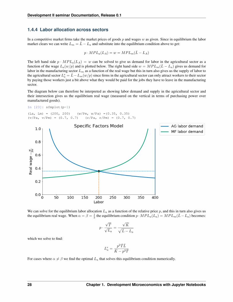
1.4.4 Labor allocation across sectors
In a competitive market firms take the market prices of goods 𝑝 and wages 𝑤 as given. Since in equilibrium the labormarket clears we can write 𝐿𝑚 = ��− 𝐿𝑎 and substitute into the equilibrium condition above to get:
𝑝 ·𝑀𝑃𝐿𝑎(𝐿𝐴) = 𝑤 = 𝑀𝑃𝐿𝑚(��− 𝐿𝐴)
The left hand side 𝑝 · 𝑀𝑃𝐿𝑎(𝐿𝐴) = 𝑤 can be solved to give us demand for labor in the agricultural sector as afunction of the wage 𝐿𝑎(𝑤/𝑝) and is plotted below. The right hand side 𝑤 = 𝑀𝑃𝐿𝑚(�� − 𝐿𝑎) gives us demand forlabor in the manufacturing sector 𝐿𝑚 as a function of the real wage but this in turn also gives us the supply of labor tothe agricultural sector 𝐿𝑠
𝑎 = ��−𝐿𝑚(𝑤/𝑝) since firms in the agricultural sector can only attract workers to their sectorby paying those workers just a bit above what they would be paid for the jobs they have to leave in the manufacturingsector.
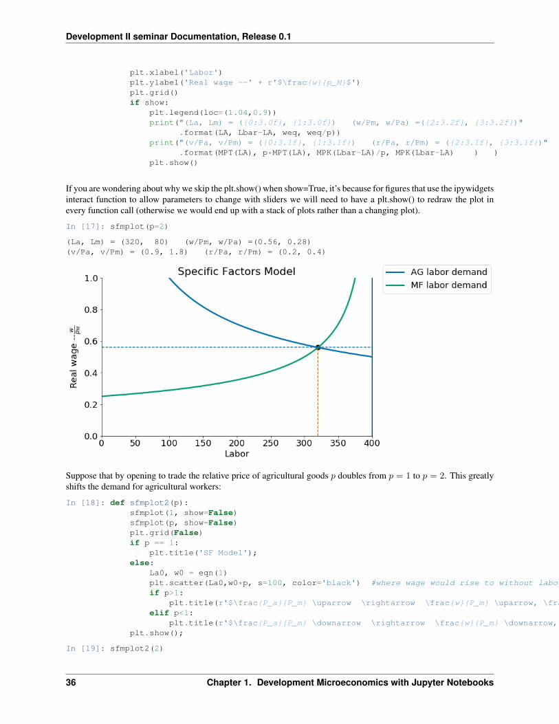
The diagram below can therefore be interpreted as showing labor demand and supply in the agricultural sector andtheir intersection gives us the equilibrium real wage (measured on the vertical in terms of purchasing power overmanufactured goods).
In [23]: sfmplot(p=1)
(La, Lm) = (200, 200) (w/Pm, w/Pa) =(0.35, 0.35)(v/Pa, v/Pm) = (0.7, 0.7) (r/Pa, r/Pm) = (0.7, 0.7)
We can solve for the equilibrium labor allocation 𝐿𝑎 as a function of the relative price 𝑝, and this in turn also gives usthe equilibrium real wage. When 𝛼 = 𝛽 = 1
2 the equilibrium condition 𝑝 ·𝑀𝑃𝐿𝑎(𝐿𝑎) = 𝑀𝑃𝐿𝑚(��−𝐿𝑎) becomes:
𝑝 ·√𝑇√𝐿𝑎
=
√��√
��− 𝐿𝑎
which we solve to find:
𝐿𝑒𝑎 =
𝑝2𝑇 ��
�� − 𝑝2𝑇
For cases where 𝛼 = 𝛽 we find the optimal 𝐿𝑎 that solves this equilibrium condition numerically.
28 Chapter 1. Development Microeconomics with Jupyter Notebooks
Development II seminar Documentation, Release 0.1
Autarky prices
Thus far we have a pretty complete model of how production allocations and real wages would be determined in asmall open economy where producers face world price ratio 𝑝. we explore comparative statics in this economy in moredetail below.
If however the economy is inititally in autarky or closed to the world then we must also consider the role of domesticconsumer preferences in the determination of domestic equilibrium product prices.
With Cobb-Douglas preferences 𝑢(𝑥, 𝑦) = 𝛾 ln(𝑥) + (1 − 𝛾) ln(𝑦) consumers demands can be written as a functionof relative price 𝑝 = 𝑃𝑎
𝑃𝑚. Setting 𝑃𝑚 = 1 to make manufacturing the numeraire good, this can be written:
𝐶𝑎(𝑝) =𝛾 · 𝐼(𝑝)
𝑝(1.1)
𝐶𝑚(𝑝) =(1 − 𝛾) · 𝐼(𝑝)(1.2)
Income 𝐼 in the expressions is given by the value of national production or GDP at these prices. Measured in manu-factured goods:
𝐼(𝑝) = 𝑝 · 𝐹 (𝑇 , 𝐿𝑎(𝑝)) + 𝐺(��, ��− 𝐿𝑎(𝑝)
By Walras’ law we only need to find the relative price at which output equals demand in one of the two product marketsso in the the code below we solve for equilibrium domestic prices from the condition 𝑄𝑎(𝑝) = 𝐶𝑎(𝑝).
For parameters 𝛼 = 𝛽 = 𝛾 = 12 , 𝑇 = �� = 100 and �� = 400 the domestic equilibrium prices are unitary:
In [24]: p_autarky(Lbar, Tbar, Kbar)
Out[24]: 1.0
And this in turn leads to an equilibrium autarky allocation with 𝐿𝑎 = 𝐿𝑚 = 200 and a real wage 𝑤𝑝 = 0.35.
In [25]: eqn(p_autarky())
Out[25]: (200.0, 0.35355339059327373)
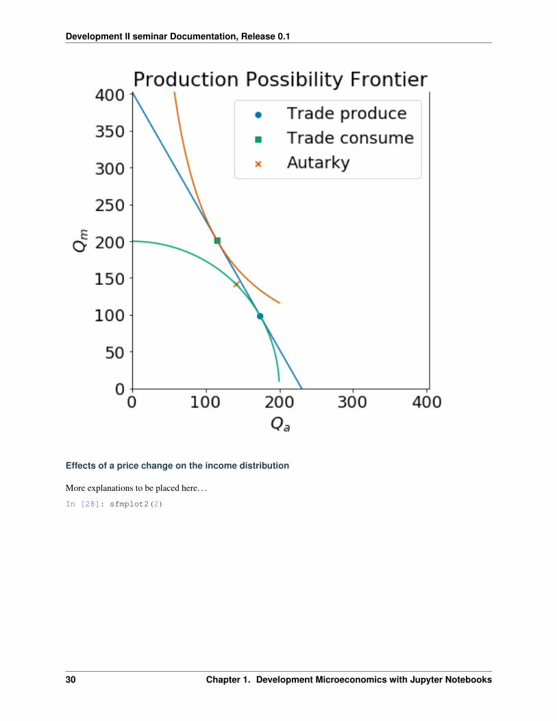
The plot below shows the autarky production and consumption point (marked by an ‘X’) as well as the new productionpoint (marked by a circle) and consumption point (marked by a square) if the country opened to trade with a worldrelative price 𝑝 = 7
4 .
Opening to trade leads the country to expand agricultural production by re-allocating labor from manufacturing toagriculture. We confirm the expected neoclassical ambiguity result which is that an increase in the relative price ofagricultural goods will lead to an increase in the real wage measured in terms of manufactured goods 𝑤
𝑝𝑚(= 𝑤 since
we have 𝑃𝑚 = 1) but a decrease in real wage measured in terms of agricultural goods or 𝑤𝑃𝑎
= 𝑤𝑝 in our notation
(since 𝑤𝑃𝑎
= 𝑤𝑝𝑚
· 𝑃𝑚
𝑃𝑎).
Diagrammatically
𝑝 ↑→ 𝑤
𝑝𝑚↑, 𝑤
𝑝𝑎↓
In [26]: pw = 7/4Lao, wo = eqn(p=pw)Lao, wo, wo/pw
Out[26]: (301.53846153846149, 0.50389110926865943, 0.28793777672494825)
In [27]: sfmtrade(p=7/4)
1.4. The Specific Factors or Ricardo-Viner Model 29
Development II seminar Documentation, Release 0.1
Effects of a price change on the income distribution
More explanations to be placed here. . .
In [28]: sfmplot2(2)
30 Chapter 1. Development Microeconomics with Jupyter Notebooks

Development II seminar Documentation, Release 0.1
## Code Section
Make sure you run the cells below FIRST. Then run the cells above
Python simulation and plots
In [1]: import numpy as npfrom scipy.optimize import fsolvenp.seterr(divide='ignore', invalid='ignore')import matplotlib.pyplot as pltfrom ipywidgets import interact, fixedimport seaborn%matplotlib inline
In [2]: plt.style.use('seaborn-colorblind')plt.rcParams["figure.figsize"] = [7,7]plt.rcParams["axes.spines.right"] = Trueplt.rcParams["axes.spines.top"] = Falseplt.rcParams["font.size"] = 18plt.rcParams['figure.figsize'] = (10, 6)plt.rcParams['axes.grid']=True
In [3]: Tbar = 100 # Fixed specific land in ag.Kbar = 100 # Fixed specific capital in manufLbar = 400 # Total number of mobile workersLbarMax = 400 # Lbar will be on slider, max value.
p = 1.00 # initial rel price of ag goods, p = Pa/Pmalpha, beta = 0.5, 0.5 # labor share in ag, manuf
For the plots we want to plot over 𝐿𝑎 and 𝐿𝑚 = ��− 𝑙𝑎:
1.4. The Specific Factors or Ricardo-Viner Model 31
Development II seminar Documentation, Release 0.1
In [4]: La = np.linspace(1, LbarMax-1,LbarMax)Lm = Lbar - La
The production functions in each sector:
In [5]: def F(La, Tbar = Tbar):return (Tbar**(1-alpha) * La**alpha)
def G(Lm, Kbar =Kbar):return (Kbar**(1-beta) * Lm**beta)
In [6]: def MPLa(La):return alpha*Tbar**(1-alpha) * La**(alpha-1)
def MPLm(Lm):return beta*Kbar**(1-beta) * Lm**(beta-1)
def MPT(La, Tbar=Tbar):return (1-alpha)*Tbar**(-alpha) * La**alpha
def MPK(Lm, Kbar=Kbar):return (1-beta)*Kbar**(-beta) * Lm**beta
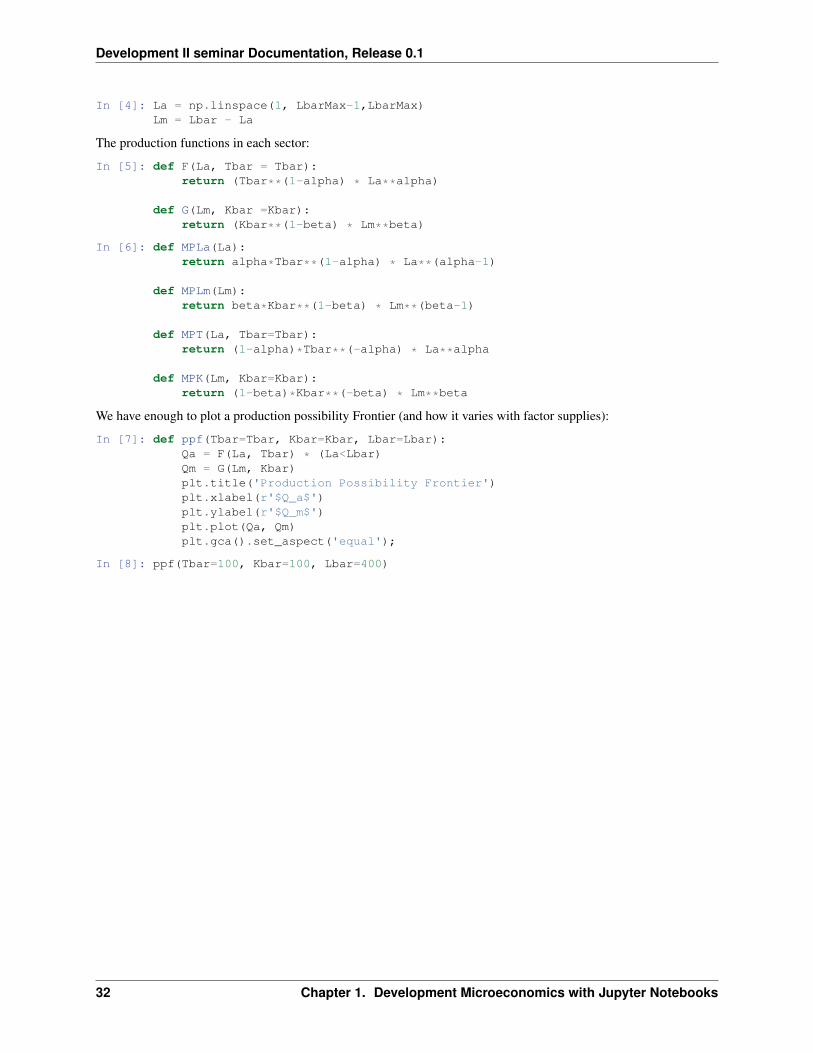
We have enough to plot a production possibility Frontier (and how it varies with factor supplies):
In [7]: def ppf(Tbar=Tbar, Kbar=Kbar, Lbar=Lbar):Qa = F(La, Tbar) * (La<Lbar)Qm = G(Lm, Kbar)plt.title('Production Possibility Frontier')plt.xlabel(r'$Q_a$')plt.ylabel(r'$Q_m$')plt.plot(Qa, Qm)plt.gca().set_aspect('equal');
In [8]: ppf(Tbar=100, Kbar=100, Lbar=400)
32 Chapter 1. Development Microeconomics with Jupyter Notebooks
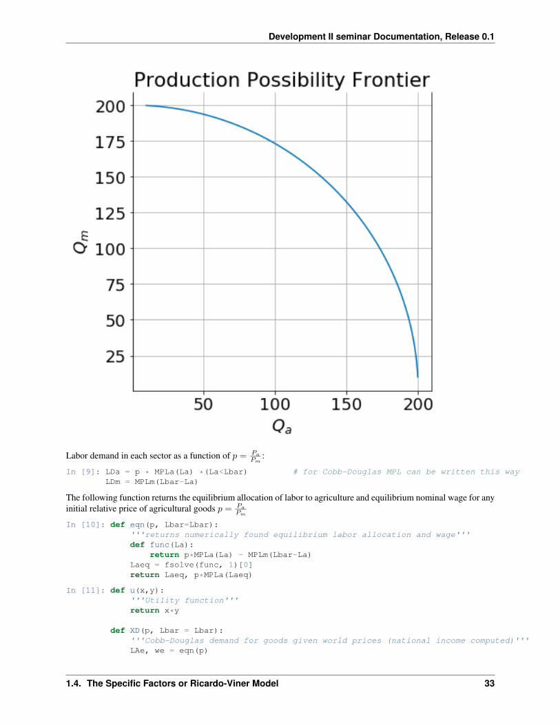
Development II seminar Documentation, Release 0.1
Labor demand in each sector as a function of 𝑝 = 𝑃𝑎
𝑃𝑚:
In [9]: LDa = p * MPLa(La) *(La<Lbar) # for Cobb-Douglas MPL can be written this wayLDm = MPLm(Lbar-La)
The following function returns the equilibrium allocation of labor to agriculture and equilibrium nominal wage for anyinitial relative price of agricultural goods 𝑝 = 𝑃𝑎
𝑃𝑚
In [10]: def eqn(p, Lbar=Lbar):'''returns numerically found equilibrium labor allocation and wage'''def func(La):
return p*MPLa(La) - MPLm(Lbar-La)Laeq = fsolve(func, 1)[0]return Laeq, p*MPLa(Laeq)
In [11]: def u(x,y):'''Utility function'''return x*y
def XD(p, Lbar = Lbar):'''Cobb-Douglas demand for goods given world prices (national income computed)'''LAe, we = eqn(p)
1.4. The Specific Factors or Ricardo-Viner Model 33
Development II seminar Documentation, Release 0.1
# gdp at world prices measured in manuf goodsgdp = p*F(LAe, Tbar = Tbar) + G(Lbar -LAe, Kbar=Kbar)return (1/2)*gdp/p, (1/2)*gdp
def indif(x, ubar):return ubar/x
In [12]: def p_autarky(Lbar=Lbar, Tbar=Tbar, Kbar=Kbar):'''Find autarky product prices. By Walras' law enough to find price thatsets excess demand in just one market'''def excessdemandA(p):
LAe, _ = eqn(p)QA = F(LAe, Tbar = Tbar)CA, CM = XD(p, Lbar=Lbar)return QA-CA
peq = fsolve(excessdemandA, 1)[0]return peq
In [13]: p_autarky()
Out[13]: 1.0
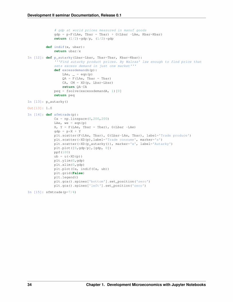
In [14]: def sfmtrade(p):Ca = np.linspace(0,200,200)LAe, we = eqn(p)X, Y = F(LAe, Tbar = Tbar), G(Lbar -LAe)gdp = p*X + Yplt.scatter(F(LAe, Tbar), G(Lbar-LAe, Tbar), label='Trade produce')plt.scatter(*XD(p),label='Trade consume', marker='s')plt.scatter(*XD(p_autarky()), marker='x', label='Autarky')plt.plot([0,gdp/p],[gdp, 0])ppf(100)ub = u(*XD(p))plt.ylim(0,gdp)plt.xlim(0,gdp)plt.plot(Ca, indif(Ca, ub))plt.grid(False)plt.legend()plt.gca().spines['bottom'].set_position('zero')plt.gca().spines['left'].set_position('zero')
In [15]: sfmtrade(p=7/4)
34 Chapter 1. Development Microeconomics with Jupyter Notebooks
Development II seminar Documentation, Release 0.1
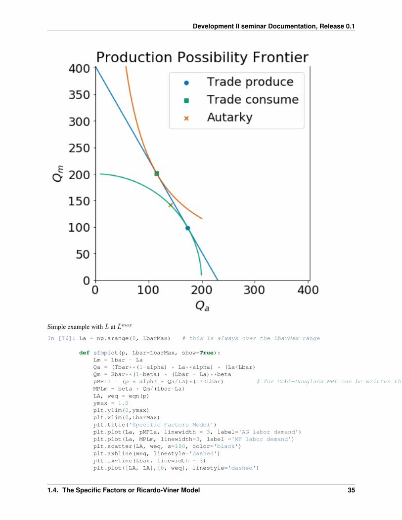
Simple example with �� at ��𝑚𝑎𝑥
In [16]: La = np.arange(0, LbarMax) # this is always over the LbarMax range
def sfmplot(p, Lbar=LbarMax, show=True):Lm = Lbar - LaQa = (Tbar**(1-alpha) * La**alpha) * (La<Lbar)Qm = Kbar**(1-beta) * (Lbar - La)**betapMPLa = (p * alpha * Qa/La)*(La<Lbar) # for Cobb-Douglass MPL can be written this wayMPLm = beta * Qm/(Lbar-La)LA, weq = eqn(p)ymax = 1.0plt.ylim(0,ymax)plt.xlim(0,LbarMax)plt.title('Specific Factors Model')plt.plot(La, pMPLa, linewidth = 3, label='AG labor demand')plt.plot(La, MPLm, linewidth=3, label ='MF labor demand')plt.scatter(LA, weq, s=100, color='black')plt.axhline(weq, linestyle='dashed')plt.axvline(Lbar, linewidth = 3)plt.plot([LA, LA],[0, weq], linestyle='dashed')
1.4. The Specific Factors or Ricardo-Viner Model 35
Development II seminar Documentation, Release 0.1
plt.xlabel('Labor')plt.ylabel('Real wage --' + r'$\frac{w}{p_M}$')plt.grid()if show:
plt.legend(loc=(1.04,0.9))print("(La, Lm) = ({0:3.0f}, {1:3.0f}) (w/Pm, w/Pa) =({2:3.2f}, {3:3.2f})"
.format(LA, Lbar-LA, weq, weq/p))print("(v/Pa, v/Pm) = ({0:3.1f}, {1:3.1f}) (r/Pa, r/Pm) = ({2:3.1f}, {3:3.1f})"
.format(MPT(LA), p*MPT(LA), MPK(Lbar-LA)/p, MPK(Lbar-LA) ) )plt.show()
If you are wondering about why we skip the plt.show() when show=True, it’s because for figures that use the ipywidgetsinteract function to allow parameters to change with sliders we will need to have a plt.show() to redraw the plot inevery function call (otherwise we would end up with a stack of plots rather than a changing plot).
In [17]: sfmplot(p=2)
(La, Lm) = (320, 80) (w/Pm, w/Pa) =(0.56, 0.28)(v/Pa, v/Pm) = (0.9, 1.8) (r/Pa, r/Pm) = (0.2, 0.4)
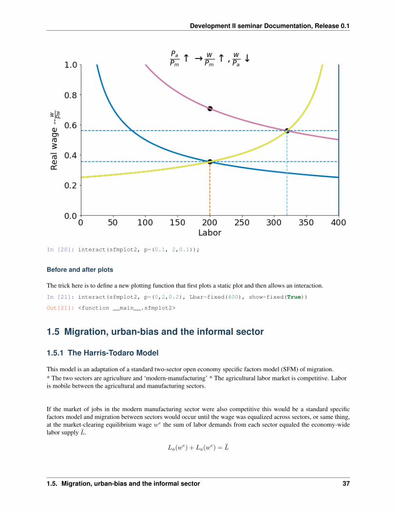
Suppose that by opening to trade the relative price of agricultural goods 𝑝 doubles from 𝑝 = 1 to 𝑝 = 2. This greatlyshifts the demand for agricultural workers:
In [18]: def sfmplot2(p):sfmplot(1, show=False)sfmplot(p, show=False)plt.grid(False)if p == 1:
plt.title('SF Model');else:
La0, w0 = eqn(1)plt.scatter(La0,w0*p, s=100, color='black') #where wage would rise to without labor movementif p>1:
plt.title(r'$\frac{P_a}{P_m} \uparrow \rightarrow \frac{w}{P_m} \uparrow, \frac{w}{P_a} \downarrow $' );elif p<1:
plt.title(r'$\frac{P_a}{P_m} \downarrow \rightarrow \frac{w}{P_m} \downarrow, \frac{w}{P_a} \uparrow $' );plt.show();
In [19]: sfmplot2(2)
36 Chapter 1. Development Microeconomics with Jupyter Notebooks
Development II seminar Documentation, Release 0.1
In [20]: interact(sfmplot2, p=(0.1, 2,0.1));
Before and after plots
The trick here is to define a new plotting function that first plots a static plot and then allows an interaction.
In [21]: interact(sfmplot2, p=(0,2,0.2), Lbar=fixed(400), show=fixed(True))
Out[21]: <function __main__.sfmplot2>
1.5 Migration, urban-bias and the informal sector
1.5.1 The Harris-Todaro Model
This model is an adaptation of a standard two-sector open economy specific factors model (SFM) of migration.* The two sectors are agriculture and ‘modern-manufacturing’ * The agricultural labor market is competitive. Laboris mobile between the agricultural and manufacturing sectors.
If the market of jobs in the modern manufacturing sector were also competitive this would be a standard specificfactors model and migration between sectors would occur until the wage was equalized across sectors, or same thing,at the market-clearing equilibrium wage 𝑤𝑒 the sum of labor demands from each sector equaled the economy-widelabor supply ��.
𝐿𝑎(𝑤𝑒) + 𝐿𝑎(𝑤𝑒) = ��
1.5. Migration, urban-bias and the informal sector 37
Development II seminar Documentation, Release 0.1
However, for institutional/political economy reasons wages in the modern manufacturing sector will be set artificiallyhigh, for example by union activity or minimum-wage policies in that sector. This high wage will lead firms in thatsector to cut back hiring but will also attract migrants to urban areas. lured by the prospect of possibly landing a high-wage job in the urban sector. Since not all migrants succeed in landing these rationed jobs however this migration willlead to the endogenous emergence of an informal urban sector in the economy and ‘urban-bias’ (a larger than efficienturban sector).
Laborers can now either stay in the rural sector to earn wage equilibrium rural wage 𝑤𝑟 or migrate to the urbanarea where they may land either in (a) the informal sector where they earn a low-productivity determined wage 𝑤𝑢
or (b) in the high-wage modern manufacturing sector where they earn the institutionally-determined wage 𝑤𝑚. Wemodel assumes that only urban dwellers can apply for modern-manufacturing and that jobs are allocated among suchapplicants by lottery whenever those jobs are in excess demand.
A fixed constant informal sector wage can be justified by assuming that the informal sector is competitive and produc-tion takes place with a simple low-productivity linear technology. Wages in that sector are then pinned to 𝑤𝑢 = 𝑎𝑢where 𝑎𝑢 is the constant marginal product of labor in the informal sector.
Migration will now take place until the rural wage is equalized to the expected wage of an urban resident:
𝑤𝑟 =𝐿𝑚(𝑤𝑚)
𝐿𝑢 + 𝐿𝑚(𝑤𝑚)· 𝑤𝑚 +
𝐿𝑢
𝐿𝑢 + 𝐿𝑚(𝑤𝑚)· 𝑤𝑢
Labor demand in each sector will depend on product prices. Without loss of generality and to simplify let’s normalize𝑃𝑟 = 1 and now call 𝑝 = 𝑃𝑟
𝑃𝑚the relative price of agricultural goods.
We can then write 𝐿𝑟(𝑤) as the solution to
𝑝 · 𝐹𝐿(𝑇 , 𝐿𝑟) = 𝑤
and labor demand 𝐿𝑚(𝑤) as the solution to
𝐺𝐿(��, 𝐿𝑚) = 𝑤
Given the assumption that jobs in the high-wage manufacturing sector are allocated by fair lottery the equilibiumprobability of getting such a job will be given simply by the share of the urban sector labor force in that sector.
If, without loss of generality we normalize the informal sector wage 𝑤𝑢 to zero (we’ll change that later) the equilbriumcondition becomes just:
𝑤𝑟 =𝐿𝑚(𝑤𝑚)
𝐿𝑢 + 𝐿𝑚(𝑤𝑚)· 𝑤𝑚
Since 𝑤𝑚 is fixed labor use in the modern manufacturing sector will be 𝐿𝑚(𝑤𝑚) and the market can be thought ofas clearing at a rural wage 𝑤𝑟 and a size of the urban informal sector 𝐿𝑢 of just the right size to dissuade any furthermigration.
Note that this condition can be re-written more simply as follows:
𝑤𝑚 · 𝐿𝑚 = 𝑤𝑟 · (��− 𝐿𝑟)
Since ��, 𝑤𝑚 and hence also 𝐿𝑚 = 𝐿𝑚(𝑤𝑚) are all fixed quantities this is an equation in two unknowns.
We can solve for the two unknowns 𝑤𝑟 and 𝐿𝑟 from a system of two equations.
The first is this last equation which is a rectangular hyperbola of the form 𝑥 · 𝑦 = 𝜅, where here 𝑥 = �� − 𝐿𝑟 and𝑦 = 𝑤𝑟).
The other equation is the competitive equilibrium condition
𝑝 · 𝐹𝐿(��𝑟, 𝐿𝑟) = 𝑤𝑟
that at a competitive optimum the rural wage 𝑤𝑟 will be given by the marginal value product of labor in agriculture.
38 Chapter 1. Development Microeconomics with Jupyter Notebooks
Development II seminar Documentation, Release 0.1
Diagram analysis
Although this is a simple system of two non-linear equations in two unknowns, it’s hard to get a tidy closed formsolution for Cobb Douglas production functions. It is easy to see the solution graphically and solve for it numerically,however.
Suppose production in the agricultural and manufacturing sectors is carried out by identical firms in each sector eachemploying the following linear homogenous Cobb-Douglas technologies:
𝐺(𝑇 , 𝐿𝑟) = 𝐴𝑟𝑇𝛼 · 𝐿1−𝛼
𝑟
𝐹 (��, 𝐿𝑚) = 𝐴𝑚��𝛽 · 𝐿1−𝛽𝑚
Labor demand in manufacturing as a function of 𝑤:
𝐿𝑚(𝑤𝑚) =
[𝐴𝑚(1 − 𝛽)��
𝑤𝑚/𝑃𝑚
] 1𝛽
and rural labor demand:
𝐿𝑟(𝑤𝑟) =
[𝐴𝑟(1 − 𝛼)𝑇
𝑤𝑟/𝑃𝑟
] 1𝛼
In [1]: import numpy as npimport matplotlib.pyplot as pltfrom ipywidgets import interactfrom scipy.optimize import bisect,newton%matplotlib inline
In [2]: Tbar = 200 # Fixed specific land in ag.Kbar = 200 # Fixed specific capital in manufLbar = 400 # Total number of mobile workersLbarMax = 400 # Lbar will be on slider, max value.A = 1p = 1.00 # initial rel price of ag goods, p = Pa/Pmalpha, beta = 0.75, 0.5 # labor share in ag, manuf
In [3]: def F(L,T, A=1, alpha=0.5):return A*(T**alpha)*(L**(1-alpha))
def G(L, K, A=1, beta=0.5):return A*(K**beta)*(L**(1-beta))
def mplr(L,T=Tbar, A=1, alpha=0.5):return (1-alpha)*F(L,T,A,alpha)/L
def mplm(L, K=Kbar, A=1, beta=0.5):return (1-beta)*G(L,K,A,beta)/L
def Lm(w):return Kbar*((p/w)*(A*(1-beta)))**(1/beta)
def expret(Lr,wm):return wm*Lm(wm)/(Lbar-Lr)
def expwage(Lr,wm,wu):return (wm*Lm(wm) + wu*(Lbar-Lm(wm)-Lr) )/(Lbar-Lr)
The efficient competitive equilibrium is given by the point where the two labor demand curves intersect. We solvefor the level of agricultural employment at which there is zero excess demand for agricultural labor. This gives anequilibrium agricultural labor demand economy-wide equilibrium wage.
1.5. Migration, urban-bias and the informal sector 39
Development II seminar Documentation, Release 0.1
In [4]: def effeq():ed = lambda L: mplr(L) - mplm(Lbar-L)LE = bisect(ed,10,Lbar-10)return mplr(LE), LE
A Harris-Todaro equilibrium is one where the rural wage equals the expected urban wage. Diagramatically the equi-librium level of rural employtment is given by the intersection of the rural labor demand curve and the rectangularhyperbola running through (𝑤𝑚, 𝐿𝑚(𝑤𝑚)).
In [5]: def harristodaro(wm,wu):LM = Lm(wm)WE, LE = effeq()hteq = lambda L: mplr(L) - (wm*LM + wu*(Lbar-LM-L) )/(Lbar-L)LR = newton(hteq, LE)WR = mplr(LR)return WR, LR, LM, WE, LE
This next function plots the diagram.
In [6]: def HTplot(wm, wu):WR, LR, LM, WE, LE = harristodaro(wm, wu)print('(wr, Lr), Lm, (we, le)=({:5.2f},{:5.0f}),{:5.0f},({:5.2f},{:5.0f},)'.format(WR, LR, LM, WE, LE))lr = np.arange(1,Lbar)lup = np.arange(LR-20, Lbar-LM+20)fig, ax = plt.subplots(figsize=(10,6))ax.plot(lr[:-50], mplr(lr[:-50]), lw=2)ax.plot(lr[50:], mplm(Lbar-lr[50:]), lw=2)ax.plot(lup, expwage(lup, wm, wu), 'k',lw=1.5)ax.vlines(LR,0,WR, linestyles="dashed")ax.vlines(Lbar-LM,0,wm,linestyles="dashed")ax.hlines(wm,Lbar,Lbar-LM, linestyles="dashed")ax.hlines(WR,LR,Lbar, linestyles="dashed")ax.plot(Lbar-LM,wm,'ob')ax.text(Lbar,wm,'$w_m$',fontsize=16)ax.text(LE,WE*1.05,'$E$',fontsize=16)ax.text(LR,WR*1.10,'$Z$',fontsize=16)ax.text(Lbar-LM-10,wm*1.05,'$D$',fontsize=16)ax.text(Lbar,WR,'$w_r$',fontsize=16)ax.plot([LE,LR, Lbar-LM],[WE, WR, wm],'ok')ax.set_xlim(0, Lbar)ax.set_ylim(0, 1.25)ax.set_xlabel(r'$c_1$', fontsize=18)ax.set_ylabel('$c_2$', fontsize=18)ax.spines['top'].set_visible(False)ax.get_xaxis().set_visible(False)ax.get_yaxis().set_visible(False)
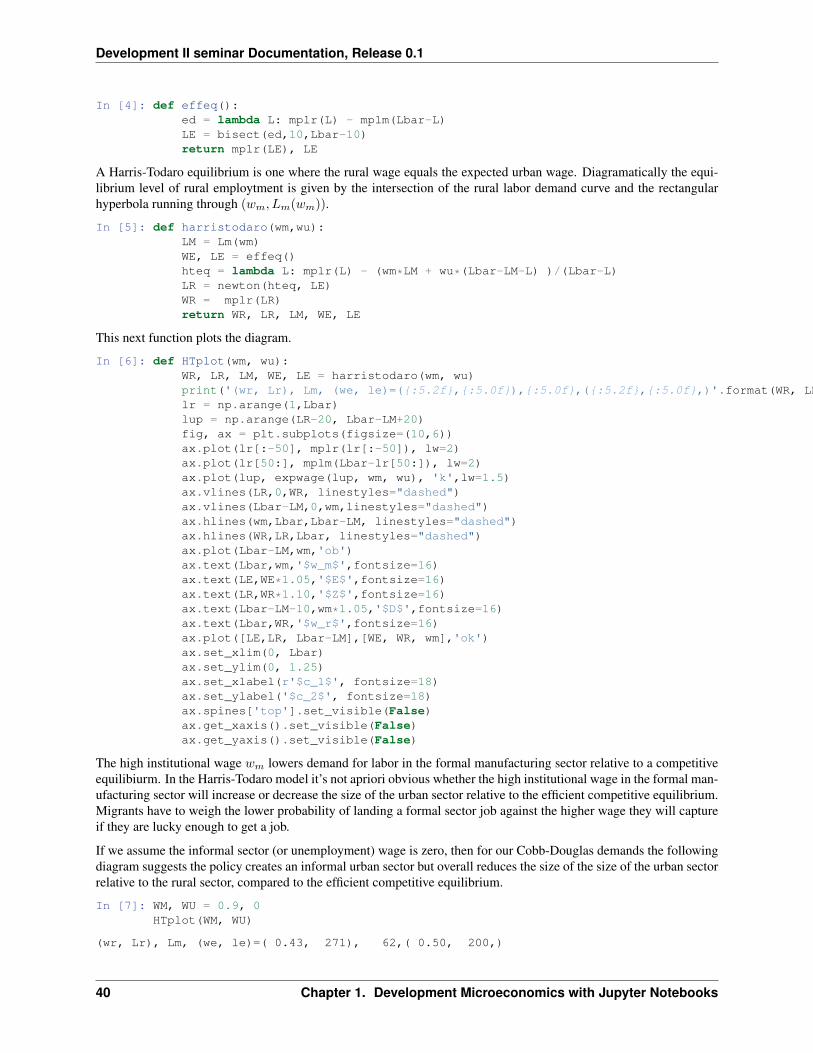
The high institutional wage 𝑤𝑚 lowers demand for labor in the formal manufacturing sector relative to a competitiveequilibiurm. In the Harris-Todaro model it’s not apriori obvious whether the high institutional wage in the formal man-ufacturing sector will increase or decrease the size of the urban sector relative to the efficient competitive equilibrium.Migrants have to weigh the lower probability of landing a formal sector job against the higher wage they will captureif they are lucky enough to get a job.
If we assume the informal sector (or unemployment) wage is zero, then for our Cobb-Douglas demands the followingdiagram suggests the policy creates an informal urban sector but overall reduces the size of the size of the urban sectorrelative to the rural sector, compared to the efficient competitive equilibrium.
In [7]: WM, WU = 0.9, 0HTplot(WM, WU)
(wr, Lr), Lm, (we, le)=( 0.43, 271), 62,( 0.50, 200,)
40 Chapter 1. Development Microeconomics with Jupyter Notebooks
Development II seminar Documentation, Release 0.1
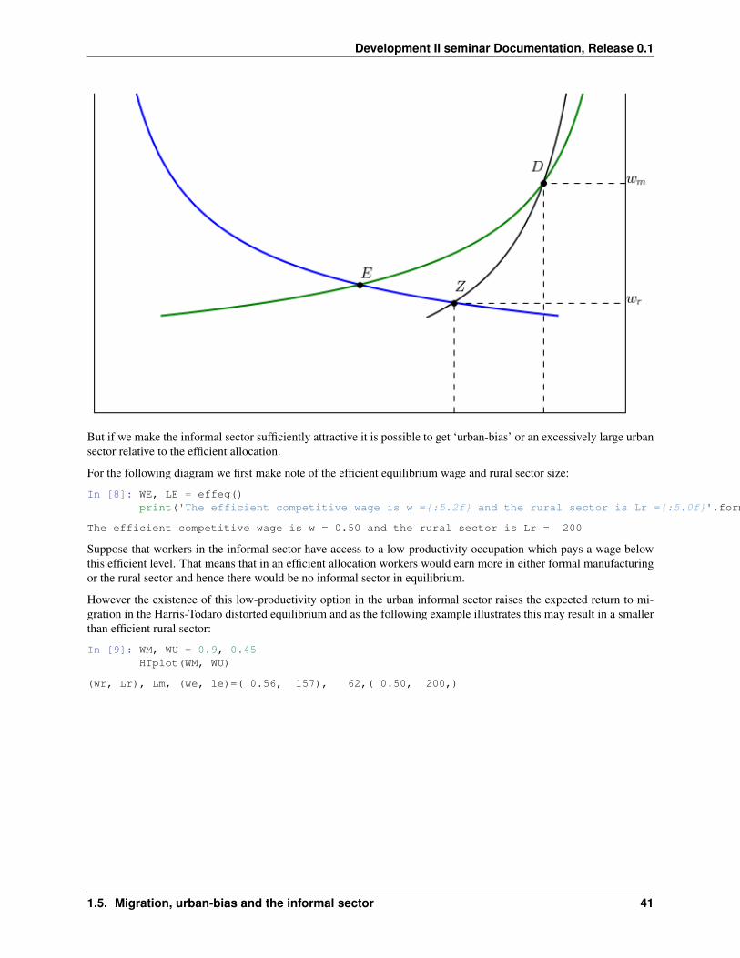
But if we make the informal sector sufficiently attractive it is possible to get ‘urban-bias’ or an excessively large urbansector relative to the efficient allocation.
For the following diagram we first make note of the efficient equilibrium wage and rural sector size:
In [8]: WE, LE = effeq()print('The efficient competitive wage is w ={:5.2f} and the rural sector is Lr ={:5.0f}'.format(WE, LE))
The efficient competitive wage is w = 0.50 and the rural sector is Lr = 200
Suppose that workers in the informal sector have access to a low-productivity occupation which pays a wage belowthis efficient level. That means that in an efficient allocation workers would earn more in either formal manufacturingor the rural sector and hence there would be no informal sector in equilibrium.
However the existence of this low-productivity option in the urban informal sector raises the expected return to mi-gration in the Harris-Todaro distorted equilibrium and as the following example illustrates this may result in a smallerthan efficient rural sector:
In [9]: WM, WU = 0.9, 0.45HTplot(WM, WU)
(wr, Lr), Lm, (we, le)=( 0.56, 157), 62,( 0.50, 200,)
1.5. Migration, urban-bias and the informal sector 41
Development II seminar Documentation, Release 0.1
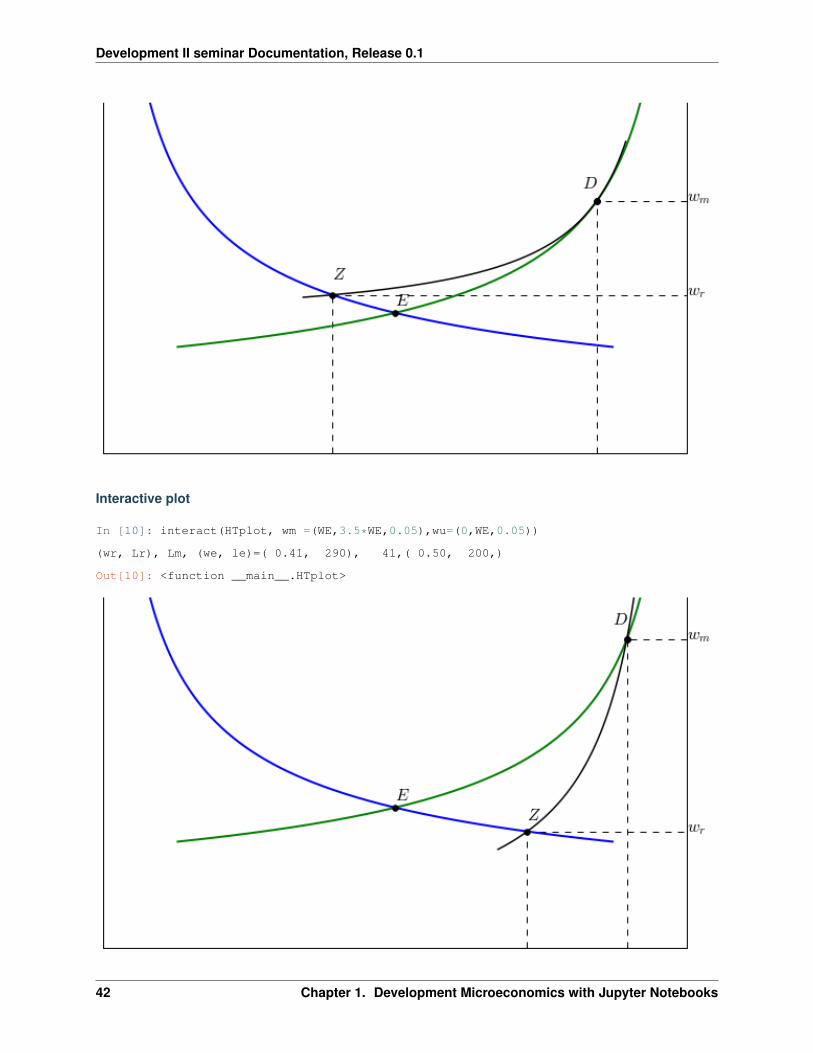
Interactive plot
In [10]: interact(HTplot, wm =(WE,3.5*WE,0.05),wu=(0,WE,0.05))
(wr, Lr), Lm, (we, le)=( 0.41, 290), 41,( 0.50, 200,)
Out[10]: <function __main__.HTplot>
42 Chapter 1. Development Microeconomics with Jupyter Notebooks
Development II seminar Documentation, Release 0.1
Extensions
Harris Todaro and Inequality
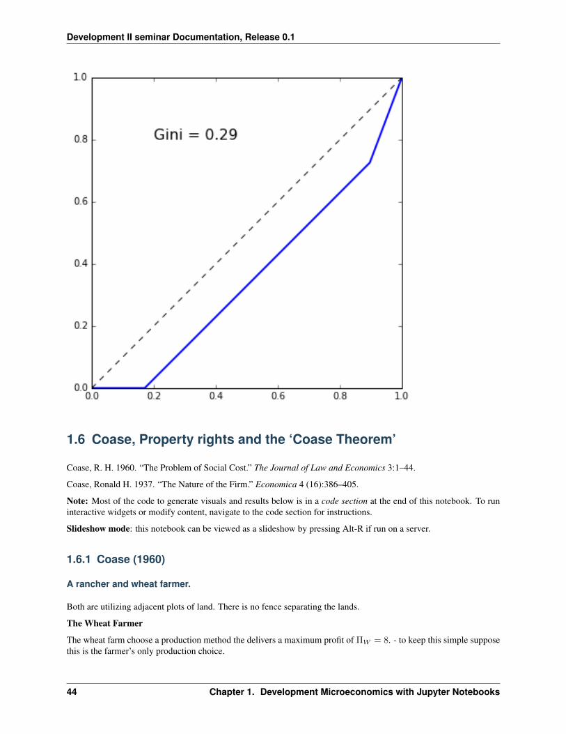
Jonathan Temple’s (2005) “Growth and Wage Inequality in a dual economy” makes some simple points about wageinequality in the HT model. He shows that in the case of $wu = $ the Gini coefficient can be written simply:
𝐺𝑖𝑛𝑖 = 𝐿𝑢(2 − 𝐿𝑢
𝑢)
where here 𝐿𝑢 is the proportion of the labor force in unemployment and 𝑢 (slightly redefining what we had above. . .or, same thing, if we normalize the total labor force to 1) and 𝑢 is urban unemployment rate or the fraction of theunemployed in the urban population (i.e. 𝑢 = 𝐿𝑢
𝐿𝑢+𝐿𝑚). From this one can prove that inequality will unambiguously
rise if one of the following statements holds if the urban unemployment rate 𝑢:
• rises, and the number of unemployed 𝐿𝑢 goes up.
• is constant, and the number of unemployed 𝐿𝑢 rises. Modern sector employment rises, and agricultural employ-ment falls.
• rises, and the number of unemployed is constant. Modern sector employment falls, and agricultural employmentrises
Another result is that rural growth (driven say by improved agricultural technology) leads to an unambiguous reductionin wage inequality. The effects of urban growth are ambiguous.
Below we plot the Lorenz curve and slightly extend Temple’s analysis to the case where ‘the unemployed’ (or informalsector workers) earn a non-zero wage. For now we simply focus on calculating the Gini numerically.
(note/fix: GINI CALCULATION DOES NOT SEEM RIGHT)
In [11]: def htlorenz(wm, wu):WR, LR, LM, WE, LE = harristodaro(wm, wu)lrp = LR/Lbarlmp = LM/Lbarlup = 1 - lrp -lmpytot = wu*(1-lrp-lmp) + WR*lrp + wm*lmpyup = wu*(1-lrp-lmp)/ytotyrp = WR*lrp/ytotymp = wm*lmp/ytotA = 0.5 - (yup*((1-lup)+ 0.5*lup)+(yrp-yup)*(lmp+0.5*lrp)+0.5*lmp*(ymp))Gini = 2*Agtext = "Gini ={:5.2f}".format(Gini)fig, ax = plt.subplots(figsize=(6,6))ax.plot([0,lup,lup+lrp,1],[0,yup,yup+yrp,1] , lw=2)ax.plot([0,1],[0,1], 'k--', lw=1)ax.text(0.2,0.8,gtext,fontsize=16)
In [12]: WM, WU = 0.9,0WR, LR, LM, WE, LE = harristodaro(WM, WU)interact(htlorenz, wm =(WE,3.5*WE,0.05),wu=(0,WE,0.05))
Out[12]: <function __main__.htlorenz>
1.5. Migration, urban-bias and the informal sector 43
Development II seminar Documentation, Release 0.1
1.6 Coase, Property rights and the ‘Coase Theorem’
Coase, R. H. 1960. “The Problem of Social Cost.” The Journal of Law and Economics 3:1–44.
Coase, Ronald H. 1937. “The Nature of the Firm.” Economica 4 (16):386–405.
Note: Most of the code to generate visuals and results below is in a code section at the end of this notebook. To runinteractive widgets or modify content, navigate to the code section for instructions.
Slideshow mode: this notebook can be viewed as a slideshow by pressing Alt-R if run on a server.
1.6.1 Coase (1960)
A rancher and wheat farmer.
Both are utilizing adjacent plots of land. There is no fence separating the lands.
The Wheat Farmer
The wheat farm choose a production method the delivers a maximum profit of Π𝑊 = 8. - to keep this simple supposethis is the farmer’s only production choice.
44 Chapter 1. Development Microeconomics with Jupyter Notebooks
Development II seminar Documentation, Release 0.1
The Rancher
Chooses herd size 𝑥 to maximize profits:
Π𝐶(𝑥) = 𝑃 · 𝐹 (𝑥) − 𝑐 · 𝑥
where 𝑃 is cattle price and 𝑐 is the cost of feeding each animal.
To simplify we allow decimal levels (but conclusions would hardly change if restrictedto integers).
First-order necessary condition for herd size 𝑥* to max profits:
𝑃 · 𝐹 ′(𝑥*) = 𝑐
**Example:* 𝑃𝑐 = 4, 𝐹 (𝑥) =√𝑥 and 𝑐 = 1
The FOC are 42√𝑥* = 1
And the rancher’s privately optimal herd size:
𝑥* = 4
The external cost
No effective barrier exists between the fields so cattle sometimes strays into the wheat farmer’s fields, trampling cropsand reducing wheat farmer’s profits.
Specifically, if rancher keeps a herd size 𝑥 net profits in wheat are reduced to :
Π𝑊 (𝑥) = Π𝑊 − 𝑑 · 𝑥2
The external cost
Suppose 𝑑 = 12
At rancher’s private optimum herd size of 𝑥* = 4 the farmer’s profit is reduced from 8 to zero:
Π𝑊 (𝑥) = Π𝑊 − 𝑑 · 𝑥2 (1.3)
= 8 − 1
2· 42 = 0(1.4)
In [11]: Pc = 4Pw = 8c = 1/2d = 1/2
CE, TE = copt(),topt()CE, TE
Out[11]: (4.0, 2.0)
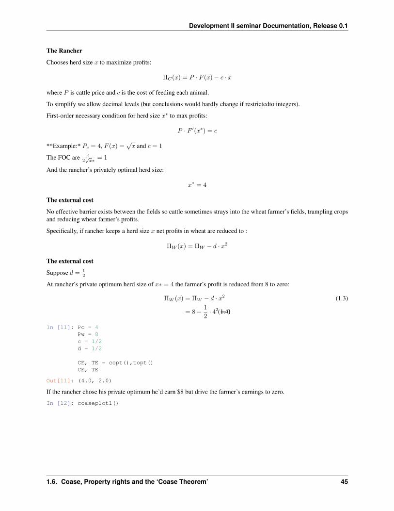
If the rancher chose his private optimum he’d earn $8 but drive the farmer’s earnings to zero.
In [12]: coaseplot1()
1.6. Coase, Property rights and the ‘Coase Theorem’ 45
Development II seminar Documentation, Release 0.1
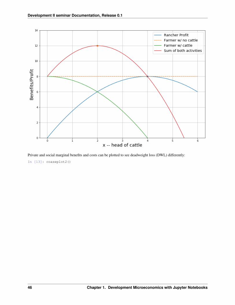
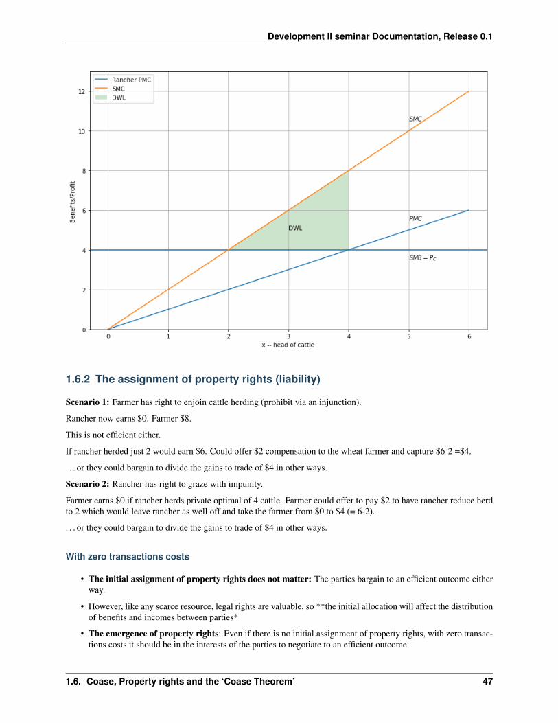
Private and social marginal benefits and costs can be plotted to see deadweight loss (DWL) differently:
In [13]: coaseplot2()
46 Chapter 1. Development Microeconomics with Jupyter Notebooks
Development II seminar Documentation, Release 0.1
1.6.2 The assignment of property rights (liability)
Scenario 1: Farmer has right to enjoin cattle herding (prohibit via an injunction).
Rancher now earns $0. Farmer $8.
This is not efficient either.
If rancher herded just 2 would earn $6. Could offer $2 compensation to the wheat farmer and capture $6-2 =$4.
. . . or they could bargain to divide the gains to trade of $4 in other ways.
Scenario 2: Rancher has right to graze with impunity.
Farmer earns $0 if rancher herds private optimal of 4 cattle. Farmer could offer to pay $2 to have rancher reduce herdto 2 which would leave rancher as well off and take the farmer from $0 to $4 (= 6-2).
. . . or they could bargain to divide the gains to trade of $4 in other ways.
With zero transactions costs
• The initial assignment of property rights does not matter: The parties bargain to an efficient outcome eitherway.
• However, like any scarce resource, legal rights are valuable, so **the initial allocation will affect the distributionof benefits and incomes between parties*
• The emergence of property rights: Even if there is no initial assignment of property rights, with zero transac-tions costs it should be in the interests of the parties to negotiate to an efficient outcome.
1.6. Coase, Property rights and the ‘Coase Theorem’ 47
Development II seminar Documentation, Release 0.1
1.6.3 With positive transactions costs
• The initial distribution of property rights typically will matter.
• It’s not so clear from this example but suppose that we had a situation with one wheat farmer and many ranchers.It might be difficult to get the ranchers
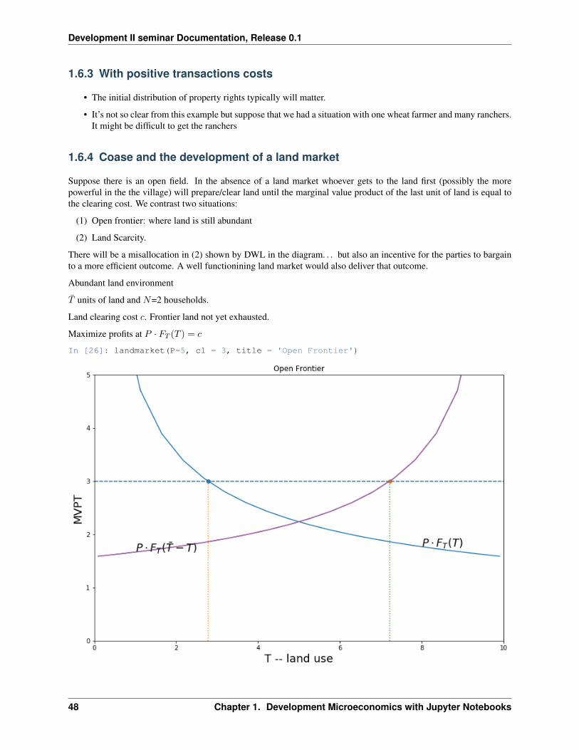
1.6.4 Coase and the development of a land market
Suppose there is an open field. In the absence of a land market whoever gets to the land first (possibly the morepowerful in the the village) will prepare/clear land until the marginal value product of the last unit of land is equal tothe clearing cost. We contrast two situations:
(1) Open frontier: where land is still abundant
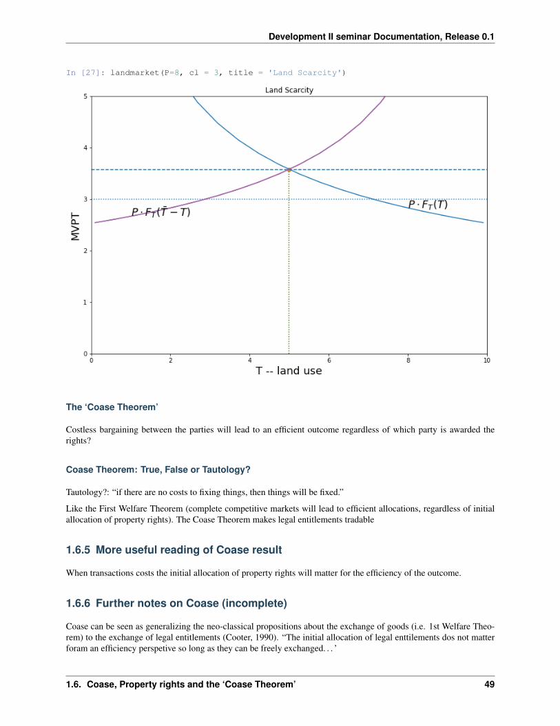
(2) Land Scarcity.
There will be a misallocation in (2) shown by DWL in the diagram. . . but also an incentive for the parties to bargainto a more efficient outcome. A well functionining land market would also deliver that outcome.
Abundant land environment
𝑇 units of land and 𝑁=2 households.
Land clearing cost 𝑐. Frontier land not yet exhausted.
Maximize profits at 𝑃 · 𝐹𝑇 (𝑇 ) = 𝑐
In [26]: landmarket(P=5, cl = 3, title = 'Open Frontier')
48 Chapter 1. Development Microeconomics with Jupyter Notebooks
Development II seminar Documentation, Release 0.1
In [27]: landmarket(P=8, cl = 3, title = 'Land Scarcity')
The ‘Coase Theorem’
Costless bargaining between the parties will lead to an efficient outcome regardless of which party is awarded therights?
Coase Theorem: True, False or Tautology?
Tautology?: “if there are no costs to fixing things, then things will be fixed.”
Like the First Welfare Theorem (complete competitive markets will lead to efficient allocations, regardless of initialallocation of property rights). The Coase Theorem makes legal entitlements tradable
1.6.5 More useful reading of Coase result
When transactions costs the initial allocation of property rights will matter for the efficiency of the outcome.
1.6.6 Further notes on Coase (incomplete)
Coase can be seen as generalizing the neo-classical propositions about the exchange of goods (i.e. 1st Welfare Theo-rem) to the exchange of legal entitlements (Cooter, 1990). “The initial allocation of legal enttilements dos not matterforam an efficiency perspetive so long as they can be freely exchanged. . . ’
1.6. Coase, Property rights and the ‘Coase Theorem’ 49

Development II seminar Documentation, Release 0.1
Suggests insuring efficiency of law is matter or removing impediments to free exchange of legal entitlements. . . . . .define entitlements clearly and enforce private contracts for their exchagne. . .
But conditions needed for efficient resource allocation. . .
Nice discussion here:
Tautology: “Costless bargaining is efficient tautologically; if I assume people can agree on socially efficient bargains,then of course they will” “The fact that side payments can be agreed upon is true even when there are no propertyrights at all.” ” In the absence of property rights, a bargain establishes a contract between parties with novel rights thatneedn’t exist ex-ante.”
“The interesting case is when transaction costs make bargaining difficult. What you should take from Coase is thatsocial efficiency can be enhanced by institutions (including the firm!) which allow socially efficient bargains to bereached by removing restrictive transaction costs, and particularly that the assignment of property rights to differentparties can either help or hinder those institutions.”
Transactions cost: time and effort to carry out a transaction.. any resources needed to negotiate and enforce contracts. . .
Coase: initial allocation of legal entitlements does not matter from an efficiency perspective so long as transactioncosts of exchange are nil. . .
Like frictionless plane in Phyisics. . . a logical construction rather than something encountered in real life..
Legal procedure to ‘lubricate’ exchange rather than allocate legal entitlement efficiently in the first place. . .
As with ordinary goods the gains from legal
The Political Coase Theorem
Acemoglu, Daron. 2003. “Why Not a Political Coase Theorem? Social Conflict, Commitment, and Politics.” Journalof Comparative Economics 31 (4):620–652.
1.6.7 Incomplete contracts
• Hard to think of all contingencies
• Hard to negotiate all contingencies
• Hard to write contracts to cover all contingencies
Incomplete contracts - silent about parties’ obligations in some states or state these only coarsely or ambiguosly
• Incomplete contracts will be revised and renegotiated as future unfolds. . . This implies
– ex-post costs (my fail to reach agreement..).
– ex-ante costs
Relationship-specific investments.. Party may be reluctant to invest because fears expropriation by the other party atrecontracting stage.. - hold up: after tenant has made investment it is sunk, landlord may hike rent to match highervalue of property (entirely due to tenant investment). . . Expecting this tenant may not invest..
“Ownership – or power – is distributed among the parties to maximise their investment incentives. Hart and Mooreshow that complementarities between the assets and the parties have important implications. If the assets are socomplementary that they are productive only when used together, they should have a single owner. Separating suchcomplementary assets does not give power to anybody, while when the assets have a single owner, the owner haspower and improved incentives.”
## Code Section Note: To re-create or modify any content go to the
50 Chapter 1. Development Microeconomics with Jupyter Notebooks
Development II seminar Documentation, Release 0.1
‘Cell’ menu above run all code cells below by choosing ‘Run All Below’. Then ‘Run all Above’ to recreate all outputabove (or go to the top and step through each code cell manually).
In [1]: import numpy as npimport matplotlib.pyplot as pltfrom scipy.optimize import fsolve%matplotlib inline
Default parameter values:
In [2]: Pc = 4Pw = 8c = 1/2d = 1/2
In [3]: def F(x,P=Pc,c=c):'''Cattle Profit'''return P*x - c*x**2
def AG(x, P=Pw):'''Wheat farm profit before crop damage'''return P*(x**0) # to return an array of len(x)
def AGD(x,P=Pw,d=d):return AG(x,P) - d*x**2
In [4]: def copt(P=Pc,c=c):'''rancher private optimum'''return P/(2*c)
def topt(P=Pc,c=c, d=d):'''Social effient optimum'''return P/(2*(c+d))
In [5]: CE, TE = copt(),topt()CE, TE
Out[5]: (4.0, 2.0)
In [6]: xx = np.linspace(0,6,100)
In [7]: def coaseplot1():fig = plt.subplots(figsize=(12,8))plt.plot(xx, F(xx), label = 'Rancher Profit' )plt.plot(xx, AG(xx), '--', label = 'Farmer w/ no cattle' )plt.plot(xx, AGD(xx), label = 'Farmer w/ cattle')plt.plot(xx, F(xx) + AGD(xx),label='Sum of both activities')plt.scatter(copt(),F(copt()))plt.scatter(topt(),F(topt()) + AGD(topt()))plt.grid()plt.ylim(0,14)plt.xlabel('x -- head of cattle', fontsize=18)plt.ylabel('Benefits/Profit', fontsize=18)plt.legend(fontsize=14);
In [8]: coaseplot1()
1.6. Coase, Property rights and the ‘Coase Theorem’ 51
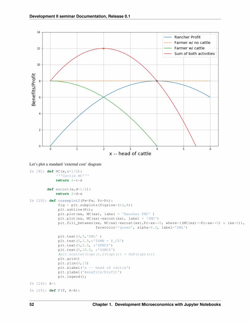
Development II seminar Documentation, Release 0.1
Let’s plot a standard ‘external cost’ diagram
In [9]: def MC(x,c=1/2):'''Cattle MC'''return 2*c*x
def excost(x,d=1/2):return 2*d*x
In [10]: def coaseplot2(Pw=Pw, Pc=Pc):fig = plt.subplots(figsize=(12,8))plt.axhline(Pc);plt.plot(xx, MC(xx), label = 'Rancher PMC' )plt.plot(xx, MC(xx)+excost(xx), label = 'SMC')plt.fill_between(xx, MC(xx)+excost(xx),Pc*xx**0, where=((MC(xx)<=Pc*xx**0) & (xx>2)),
facecolor='green', alpha=0.2, label='DWL')
plt.text(3,5,'DWL' )plt.text(5,3.5,r'$SMB = P_C$')plt.text(5,5.5, r'$PMC$')plt.text(5,10.5, r'$SMC$')#plt.scatter(topt(),G(topt()) + AGD(topt()))plt.grid()plt.ylim(0,13)plt.xlabel('x -- head of cattle')plt.ylabel('Benefits/Profit')plt.legend();
In [14]: A=1
In [15]: def F(T, A=A):
52 Chapter 1. Development Microeconomics with Jupyter Notebooks
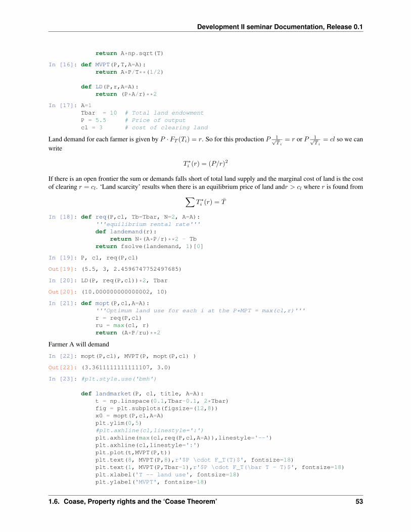
Development II seminar Documentation, Release 0.1
return A*np.sqrt(T)
In [16]: def MVPT(P,T,A=A):return A*P/T**(1/2)
def LD(P,r,A=A):return (P*A/r)**2
In [17]: A=1Tbar = 10 # Total land endowmentP = 5.5 # Price of outputcl = 3 # cost of clearing land
Land demand for each farmer is given by 𝑃 · 𝐹𝑇 (𝑇𝑖) = 𝑟. So for this production 𝑃 1√𝑇 𝑖
= 𝑟 or 𝑃 1√𝑇 𝑖
= 𝑐𝑙 so we canwrite
𝑇 *𝑖 (𝑟) = (𝑃/𝑟)2
If there is an open frontier the sum or demands falls short of total land supply and the marginal cost of land is the costof clearing 𝑟 = 𝑐𝑙. ‘Land scarcity’ results when there is an equilibrium price of land and𝑟 > 𝑐𝑙 where 𝑟 is found from∑
𝑇 *𝑖 (𝑟) = 𝑇
In [18]: def req(P,cl, Tb=Tbar, N=2, A=A):'''equilibrium rental rate'''def landemand(r):
return N*(A*P/r)**2 - Tbreturn fsolve(landemand, 1)[0]
In [19]: P, cl, req(P,cl)
Out[19]: (5.5, 3, 2.4596747752497685)
In [20]: LD(P, req(P,cl))*2, Tbar
Out[20]: (10.000000000000002, 10)
In [21]: def mopt(P,cl,A=A):'''Optimum land use for each i at the P*MPT = max(cl,r)'''r = req(P,cl)ru = max(cl, r)return (A*P/ru)**2
Farmer A will demand
In [22]: mopt(P,cl), MVPT(P, mopt(P,cl) )
Out[22]: (3.3611111111111107, 3.0)
In [23]: #plt.style.use('bmh')
def landmarket(P, cl, title, A=A):t = np.linspace(0.1,Tbar-0.1, 2*Tbar)fig = plt.subplots(figsize=(12,8))x0 = mopt(P,cl,A=A)plt.ylim(0,5)#plt.axhline(cl,linestyle=':')plt.axhline(max(cl,req(P,cl,A=A)),linestyle='--')plt.axhline(cl,linestyle=':')plt.plot(t,MVPT(P,t))plt.text(8, MVPT(P,8),r'$P \cdot F_T(T)$', fontsize=18)plt.text(1, MVPT(P,Tbar-1),r'$P \cdot F_T(\bar T - T)$', fontsize=18)plt.xlabel('T -- land use', fontsize=18)plt.ylabel('MVPT', fontsize=18)
1.6. Coase, Property rights and the ‘Coase Theorem’ 53
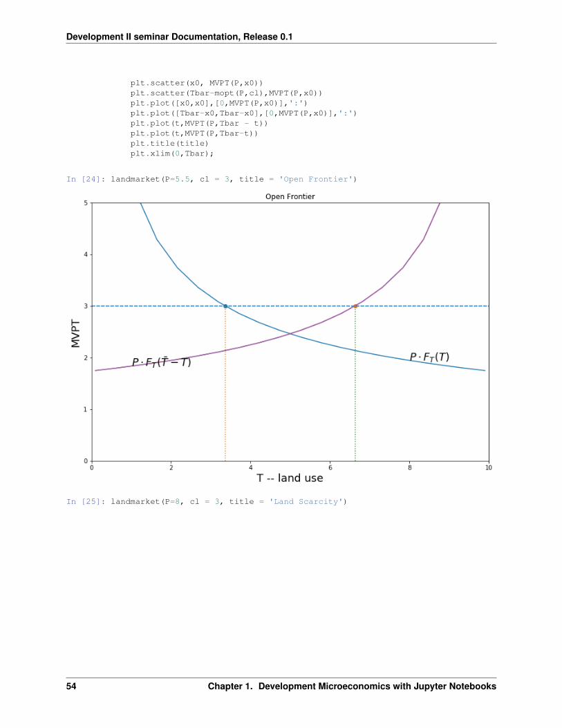
Development II seminar Documentation, Release 0.1
plt.scatter(x0, MVPT(P,x0))plt.scatter(Tbar-mopt(P,cl),MVPT(P,x0))plt.plot([x0,x0],[0,MVPT(P,x0)],':')plt.plot([Tbar-x0,Tbar-x0],[0,MVPT(P,x0)],':')plt.plot(t,MVPT(P,Tbar - t))plt.plot(t,MVPT(P,Tbar-t))plt.title(title)plt.xlim(0,Tbar);
In [24]: landmarket(P=5.5, cl = 3, title = 'Open Frontier')
In [25]: landmarket(P=8, cl = 3, title = 'Land Scarcity')
54 Chapter 1. Development Microeconomics with Jupyter Notebooks
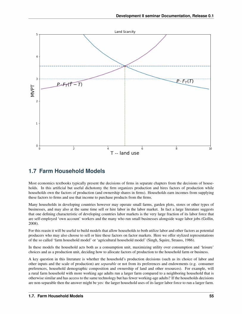
Development II seminar Documentation, Release 0.1
1.7 Farm Household Models
Most economics textbooks typically present the decisions of firms in separate chapters from the decisions of house-holds. In this artificial but useful dichotomy the firm organizes production and hires factors of production whilehouseholds own the factors of production (and ownership shares in firms). Households earn incomes from supplyingthese factors to firms and use that income to purchase products from the firms.
Many households in developing countries however may operate small farms, garden plots, stores or other types ofbusinesses, and may also at the same time sell or hire labor in the labor market. In fact a large literature suggeststhat one defining characteristic of developing countries labor markets is the very large fraction of its labor force thatare self-employed ‘own account’ workers and the many who run small businesses alongside wage labor jobs (Gollin,2008).
For this reasin it will be useful to build models that allow households to both utilize labor and other factors as potentialproducers who may also choose to sell or hire these factors on factor markets. Here we offer stylized representationsof the so called ‘farm household model’ or ‘agricultural household model’ (Singh, Squire, Strauss, 1986).
In these models the household acts both as a consumption unit, maximizing utility over consumption and ‘leisure’choices and as a production unit, deciding how to allocate factors of production to the household farm or business.
A key question in this literature is whether the household’s production decisions (such as its choice of labor andother inputs and the scale of production) are separable or not from its preferences and endowments (e.g. consumerpreferences, household demographic composition and ownership of land and other resources). For example, willa rural farm household with more working age adults run a larger farm compared to a neighboring household that isotherwise similar and has access to the same technology but has fewer working-age adults? If the households decisionsare non-separable then the answer might be yes: the larger household uses of its larger labor force to run a larger farm.
1.7. Farm Household Models 55
Development II seminar Documentation, Release 0.1
When households are embedded in well functioning competitive markets however we tend to expect the household’sdecisions to become separable:
• Household as a profit-maximizing firm: acting as a profit-maximizing firm the household first optimallychooses labor and other input allocations to extract maximum profit income from the farm.
• Household as a consumption unit: the household makes optimal choices over consumption and leisure subjectto its income budget which includes income from selling its labor endowment and maximized profits from thehousehold as a firm.
In the simple example above of two otherwise identical households the separable farm household model would predictthat both households run farms of similar size and use wage labor markets to equalize land-labor ratios and hencemarginal products of labor across farms. The larger household would be a net seller of labor on the market comparedto the smaller household.
Without the separation property the common approach of many studies to separately estimate consumer demand fromoutput supply functions is no longer valid.
Another way to state the separation hypothesis is that if they have access to markets the marginal production decisionsof farms (and firms more generally) should not depend on their owners’ ownership of tradable factors (except in so faras it might raise their overal income) or their preferences in consumption. When markets are complete then productiondecisions will be separable, the price mechanism will equalize the marginal products of factors across uses, and theinitial distribution of tradable factors should not matter for allocative efficiency (the first and second welfare theorems).Much of modern micro-development since at least the mid 1960s however is concerned with how transactions costs,asymmetric information, conflict and costly enforcement can lead to market frictions and imperfections that makeproduction decisions non-separable, which then means that the initial distribution of property rights (over land andother tradable factors) may in fact well matter for determining the patterns of production organization and its efficiencyin general equilibrium. A good example of such analysis is Eswaran and Kotwal (1986) paper on “Access to Capitaland Agrarian production organization,” which explores how the combination of transaction costs in labor hiring andin access to capital can lead to a theory of endogenous class structure or occupational choice which can changedramatically depending on the initial distribution of property rights.
1.7.1 The Chayanovian Household
We’ll start with a non-separable model, inspired by the work of the Russian agronomist Alexander Chayanov whoseearly 20th century ideas and writings on “the peasant economy” became widely influential in anthropology, economics,and other fields. Chayanov played a role in the Soviet agrarian reforms but his focus on the importance of the householdeconomy led him to be (presciently) skeptical of the appropriateness and efficiency of large-scale Soviet farms. Hewas arrested, sent to a labor camp and later executed.
The following model is not anywhere as rich as Chayanov’s description of the peasant household economy but insteada stripped down version close in spirit to Amartya Sen’s (1966) adaptation.
Farm household 𝑖 has land and labor endowment (𝑇𝑖, ��𝑖). We can assume that it can buy and sell the agriculturalproduct at a market price 𝑝 but in practice we will model the household as self-sufficient and cut off from the marketfor land and labor. The household (which we treat as a single decision-making unit for now) allocates labor maximizesutility over consumption and leisure
max𝑐𝑖,𝑙𝑖
𝑈(𝑐𝑖, 𝑙𝑖)
Although we haven’t included it above, we think of the utility function 𝑈(𝑐𝑖, 𝑙𝑖;𝐴) as depending on ‘preferenceshifters’ 𝐴 which might include such things as the household’s demographic composition or things that affect it’spreference for leisure over consumption).
The household maximizes this utility subject to the constraints that consumption 𝑐𝑖 not exceed output and that the sumof hours in production 𝐿𝑖 plus hours in leisure 𝑙𝑖 not exceed the household’s labor endowment ��𝑖
𝑐𝑖 ≤ 𝐹 (𝑇𝑖, 𝐿𝑖)
56 Chapter 1. Development Microeconomics with Jupyter Notebooks
Development II seminar Documentation, Release 0.1
𝐿𝑖 + 𝑙𝑖 ≤ ��𝑖
Substituting the constraints into the objective allows one to redefine the problem as one of choosing the right allocationof labor to production:
max𝐿𝑖
𝑈(𝐹 (𝑇𝑖, 𝐿𝑖), ��𝑖 − 𝐿𝑖)
From the first order necessary conditions we obtain
𝑈𝑐 · 𝐹𝐿 = 𝑈𝑙
which states that the farm household should allocated labor to farm production up to the point where the marginalutility benefit of additional consumption 𝑈𝑐 · 𝐹𝐿 equals the opportunity cost of leisure.
Since the household sets the marginal product of labor (or shadow price of labor) equal to the marginal rate of sub-stitution between leisure and consumption 𝐹𝐿 = 𝑈𝑙/𝑈𝑐 and the latter is clearly affected by ‘preference shifters’ 𝐴and also by the household’s land endowment. The shadow price of labor will hence differ across households that areotherwise similar (say in their access to production technology and farming skill). For example households with alarger endowment of labor will run larger farms.
It will be useful to draw things in leisure-consumption space. Leisure is measured on the horizontal from left to rightwhich then means that labor 𝐿 allocated to production can be measured from right to left with an origin starting at theendowment point ��𝑖
To fix ideas with a concrete example assume farm household 𝑖 has Cobb-Douglas preferences over consumption andleisure:
𝑈(𝑐, 𝑙) = 𝑐𝛽𝑙1−𝛽
and its production technology is a simple constant returns to scale Cobb-Douglas production function of the form:
𝐹 (𝑇𝑖, 𝐿𝑖) = 𝑇𝛼𝑖 𝐿
1−𝛼𝑖
The marginal product of labor 𝐹𝐿 which the literature frequently refers to as the shadow price of labor will be givenby:
𝐹𝐿(𝑇𝑖, 𝐿𝑖) = (1 − 𝛼)
[𝑇𝑖
𝐿𝑖
]𝛼The first order necessary condition can therefore be solved for and for these Cobb-Douglas forms we get a rathersimple and tidy solution to the optimal choice of leisure
𝑙* =𝑎 · ��1 + 𝑎
where 𝑎 = 1−𝛽𝛽·(1−𝛼)
1.7.2 Graphical analysis
(Note: formulas and plots work for default parameters but not checked for other values.)
In [1]: %matplotlib inlineimport matplotlib.pyplot as pltimport numpy as npfrom ipywidgets import interact
1.7. Farm Household Models 57
Development II seminar Documentation, Release 0.1
In [2]: ALPHA = 0.5BETA = 0.7TBAR = 100LBAR = 100
def F(T,L,alpha=ALPHA):return (T**alpha)*(L**(1-alpha))
def FL(T,L,alpha=ALPHA):"""Shadow price of labor"""return (1-alpha)*F(T,L,alpha=ALPHA)/L
def FT(T,L,alpha=ALPHA):"""Shadow price of labor"""return alpha*F(T,L,alpha=ALPHA)/T
def U(c, l, beta=BETA):return (c**beta)*(l**(1-beta))
def indif(l, ubar, beta=BETA):return ( ubar/(l**(1-beta)) )**(1/beta)
def leisure(Lbar,alpha=ALPHA, beta=BETA):a = (1-alpha)*beta/(1-beta)return Lbar/(1+a)
def HH(Tbar,Lbar,alpha=ALPHA, beta=BETA):"""Household optimum leisure, consumption and utility"""a = (1-alpha)*beta/(1-beta)leisure = Lbar/(1+a)output = F(Tbar,Lbar-leisure, alpha)utility = U(output, leisure, beta)return leisure, output, utility
In [3]: def chayanov(Tbar,Lbar,alpha=ALPHA, beta=BETA):leis = np.linspace(0.1,Lbar,num=100)q = F(Tbar,Lbar-leis,alpha)l_opt, Q, U = HH(Tbar, Lbar, alpha, beta)print("Leisure, Consumption, Utility =({:5.2f},{:5.2f},{:5.2f})"
.format(l_opt, Q, U))print("shadow price labor:{:5.2f}".format(FL(Tbar,Lbar-l_opt,beta)))c = indif(leis,U,beta)fig, ax = plt.subplots(figsize=(8,8))ax.plot(leis, q, lw=2.5)ax.plot(leis, c, lw=2.5)ax.plot(l_opt,Q,'ob')ax.vlines(l_opt,0,Q, linestyles="dashed")ax.hlines(Q,0,l_opt, linestyles="dashed")ax.set_xlim(0, 110)ax.set_ylim(0, 150)ax.set_xlabel(r'$l - leisure$', fontsize=16)ax.set_ylabel('$c - consumption$', fontsize=16)ax.spines['right'].set_visible(False)ax.spines['top'].set_visible(False)ax.grid()ax.set_title("Chayanovian Household Optimum")plt.show()
In [4]: chayanov(TBAR,LBAR,0.5,0.5)
58 Chapter 1. Development Microeconomics with Jupyter Notebooks
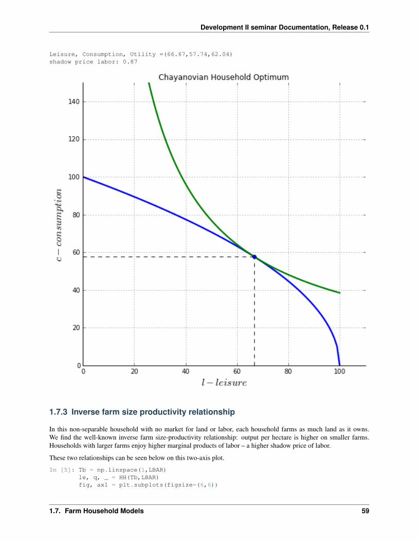
Development II seminar Documentation, Release 0.1
Leisure, Consumption, Utility =(66.67,57.74,62.04)shadow price labor: 0.87
1.7.3 Inverse farm size productivity relationship
In this non-separable household with no market for land or labor, each household farms as much land as it owns.We find the well-known inverse farm size-productivity relationship: output per hectare is higher on smaller farms.Households with larger farms enjoy higher marginal products of labor – a higher shadow price of labor.
These two relationships can be seen below on this two-axis plot.
In [5]: Tb = np.linspace(1,LBAR)le, q, _ = HH(Tb,LBAR)fig, ax1 = plt.subplots(figsize=(6,6))
1.7. Farm Household Models 59
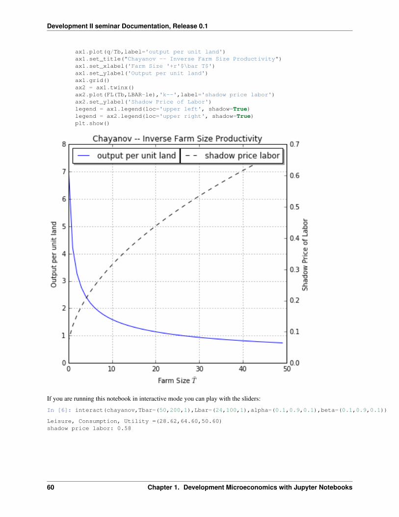
Development II seminar Documentation, Release 0.1
ax1.plot(q/Tb,label='output per unit land')ax1.set_title("Chayanov -- Inverse Farm Size Productivity")ax1.set_xlabel('Farm Size '+r'$\bar T$')ax1.set_ylabel('Output per unit land')ax1.grid()ax2 = ax1.twinx()ax2.plot(FL(Tb,LBAR-le),'k--',label='shadow price labor')ax2.set_ylabel('Shadow Price of Labor')legend = ax1.legend(loc='upper left', shadow=True)legend = ax2.legend(loc='upper right', shadow=True)plt.show()
If you are running this notebook in interactive mode you can play with the sliders:
In [6]: interact(chayanov,Tbar=(50,200,1),Lbar=(24,100,1),alpha=(0.1,0.9,0.1),beta=(0.1,0.9,0.1))
Leisure, Consumption, Utility =(28.62,64.60,50.60)shadow price labor: 0.58
60 Chapter 1. Development Microeconomics with Jupyter Notebooks
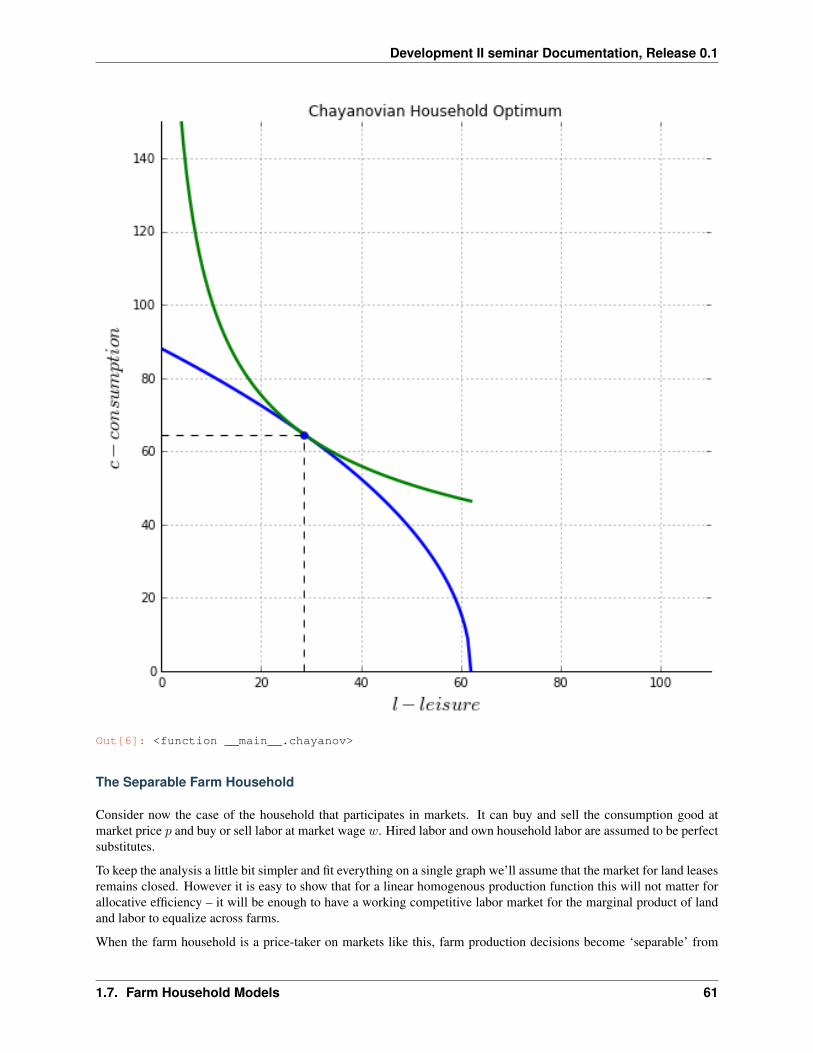
Development II seminar Documentation, Release 0.1
Out[6]: <function __main__.chayanov>
The Separable Farm Household
Consider now the case of the household that participates in markets. It can buy and sell the consumption good atmarket price 𝑝 and buy or sell labor at market wage 𝑤. Hired labor and own household labor are assumed to be perfectsubstitutes.
To keep the analysis a little bit simpler and fit everything on a single graph we’ll assume that the market for land leasesremains closed. However it is easy to show that for a linear homogenous production function this will not matter forallocative efficiency – it will be enough to have a working competitive labor market for the marginal product of landand labor to equalize across farms.
When the farm household is a price-taker on markets like this, farm production decisions become ‘separable’ from
1.7. Farm Household Models 61
Development II seminar Documentation, Release 0.1
farm consumption decisions. The farm household can make its optimal decisions as a profit-maximizing farm and thenseparately choose between consumption and leisure subject to an income constraint.
So the household’s problem can be boiled down to:
max𝑐,𝑙
𝑈(𝑐, 𝑙)
𝑠.𝑡.
𝑝 · 𝑐 ≤ 𝑝𝐹 (𝑇𝑖, 𝐿*) + 𝑤 · (��𝑖 − 𝑙)
This last constraint states that what the household spends on consumption cannot exceed the value of farm sales at aprofit maximizing optimum plus wage income from labor sold to the market. This last constraint can also be rewrittenas:
𝑝 · 𝑐 + 𝑤 · 𝑙 ≤ Π(𝑇𝑖, 𝑤, 𝑝) + 𝑤 · ��𝑖
where Π(𝑇𝑖, 𝑤, 𝑝) = 𝑝 · 𝐹 (𝑇𝑖, 𝐿*𝑖 ) − 𝑤 · 𝐿*
𝑖 is the maximized value of farm profits and 𝐿*𝑖 is the optimal quantity of
labor that achieves that maximum.
In other words the farm household can be thought of as maximizing profits by choosing an optimal labor input into thefarm 𝐿*
𝑖 which will be satisfied with own and/or hired labor. The household then maximizes utility from consumptionand leisure subject to the constraint that it not spend more on consumption and leisure as its income which is made upof farm profits (a return to land) and the market value of it’s labor endowment.
In this last description the household is thought of as buying leisure at its market wage opportunity cost.
The efficient competitive farm
As a production enterprise the farm acts to maximize farm profits $pF( _i,L_i) - w ·𝐿_𝑖$.𝑇ℎ𝑒𝑓𝑖𝑟𝑠𝑡 −𝑜𝑟𝑑𝑒𝑟𝑛𝑒𝑐𝑒𝑠𝑠𝑎𝑟𝑦𝑐𝑜𝑛𝑑𝑖𝑡𝑖𝑜𝑛𝑓𝑜𝑟𝑎𝑛𝑖𝑛𝑡𝑒𝑟𝑖𝑜𝑟𝑜𝑝𝑡𝑖𝑚𝑢𝑚𝑖𝑠 :The separation property is immediately apparent from thisfirst order condition, as this equation alone is enough to determine the farm’s optimum labor demand which dependsonly on the production technology and the market wage, and not at all on household preferences. While the quantity oflabor demanded here does depend on the households’ ownership of land, with a functioning labor market the numberof workers per unit land will be the same across all farms and hence also independent of household land endowment.
For the Cobb-Douglas production function, optimal labor demand can then be solved to be:
𝐿*𝑖 = 𝑇𝑖 ·
[𝑝(1 − 𝛼)
𝑤
] 1𝛼
Substituting this value into the profit function we can find an expression for farm profits Π(𝑇𝑖, 𝑤, 𝑝) as a function ofthe market product price and wage and the farm’s land holding. If we had allowed for hiring on both land and labormarkets we would have found zero profits with this linear homogenous technology so in this context where there is noworking land market, profits are just like a competitively determined rent to non-traded land (equal in value to whatthe same household would have earned on its land endowment had the land market been open).
Note how the optimal allocation of labor to the farm is independent of the size of the household ��𝑖 and householdpreferences. If we had allowed for a competitive land market the labor allocation would also have been independentof the household’s
Household demand for consumption and leisure is very simple given this Cobb-Douglas utility:
𝑐*(𝑤) = 𝛽 · 𝐼
𝑙*(𝑤) = (1 − 𝛽) · 𝐼𝑤
62 Chapter 1. Development Microeconomics with Jupyter Notebooks
Development II seminar Documentation, Release 0.1
where household income 𝐼 is given by the sum of farm profits and the market value of the factor endowment:
𝐼 = Π(𝑤, 𝑇 ) + 𝑤 · ��
In what follows we shall normalize the product price 𝑝 to unity. This is without loss of generality as all that matters forreal allocations is the relative price of labor (or leisure) relative to output, or the real wage 𝑤
𝑝 . So in all the expressionsthat follow when we see 𝑤 it should be thought of as 𝑤
𝑝
In [7]: def farm_optimum(Tbar, w, alpha=ALPHA, beta=BETA):"""returns optimal labor demand and profits"""LD = Tbar * ((1-alpha)/w)**(1/alpha)profit = F(Tbar, LD) - w*LDreturn LD, profit
def HH_optimum(Tbar, Lbar, w, alpha=ALPHA, beta=BETA):"""returns optimal consumption, leisure and utility.
Simple Cobb-Douglas choices from calculated income """_, profits = farm_optimum(Tbar, w, alpha)income = profits + w*Lbarconsumption = beta * incomeleisure = (1-beta) * income/wutility = U(consumption, leisure, beta)return consumption, leisure, utility
Let’s assume the market real wage starts at unity:
In [8]: W = 1
In [9]: def plot_production(Tbar,Lbar,w):lei = np.linspace(1, Lbar)q = F(Tbar, Lbar-lei)ax.plot(lei, q, lw=2.5)ax.spines['right'].set_visible(False)ax.spines['top'].set_visible(False)
In [10]: def plot_farmconsumption(Tbar, Lbar, w, alpha=ALPHA, beta=BETA):lei = np.linspace(1, Lbar)LD, profits = farm_optimum(Tbar, w)q_opt = F(Tbar,LD)yline = profits + w*Lbar - w*leic_opt, l_opt, u_opt = HH_optimum(Tbar, Lbar, w)
ax.plot(Lbar-LD,q_opt,'ob')ax.plot(lei, yline)ax.plot(lei, indif(lei,u_opt, beta),'k')ax.plot(l_opt, c_opt,'ob')ax.vlines(l_opt,0,c_opt, linestyles="dashed")ax.hlines(c_opt,0,l_opt, linestyles="dashed")ax.vlines(Lbar - LD,0,q_opt, linestyles="dashed")ax.hlines(profits,0,Lbar, linestyles="dashed")ax.vlines(Lbar,0,F(Tbar,Lbar))ax.hlines(q_opt,0,Lbar, linestyles="dashed")ax.text(Lbar+1,profits,r'$\Pi ^*$',fontsize=16)ax.text(Lbar+1,q_opt,r'$F(\bar T, L^{*})$',fontsize=16)ax.text(-6,c_opt,r'$c^*$',fontsize=16)
ax.annotate('',(Lbar-LD,2),(Lbar,2),arrowprops={'arrowstyle':'->'})ax.text((2*Lbar-LD)/2,3,r'$L^{*}$',fontsize=16)
ax.text(l_opt/2,8,'$l^*$',fontsize=16)ax.annotate('',(0,7),(l_opt,7),arrowprops={'arrowstyle':'<-'})
1.7. Farm Household Models 63
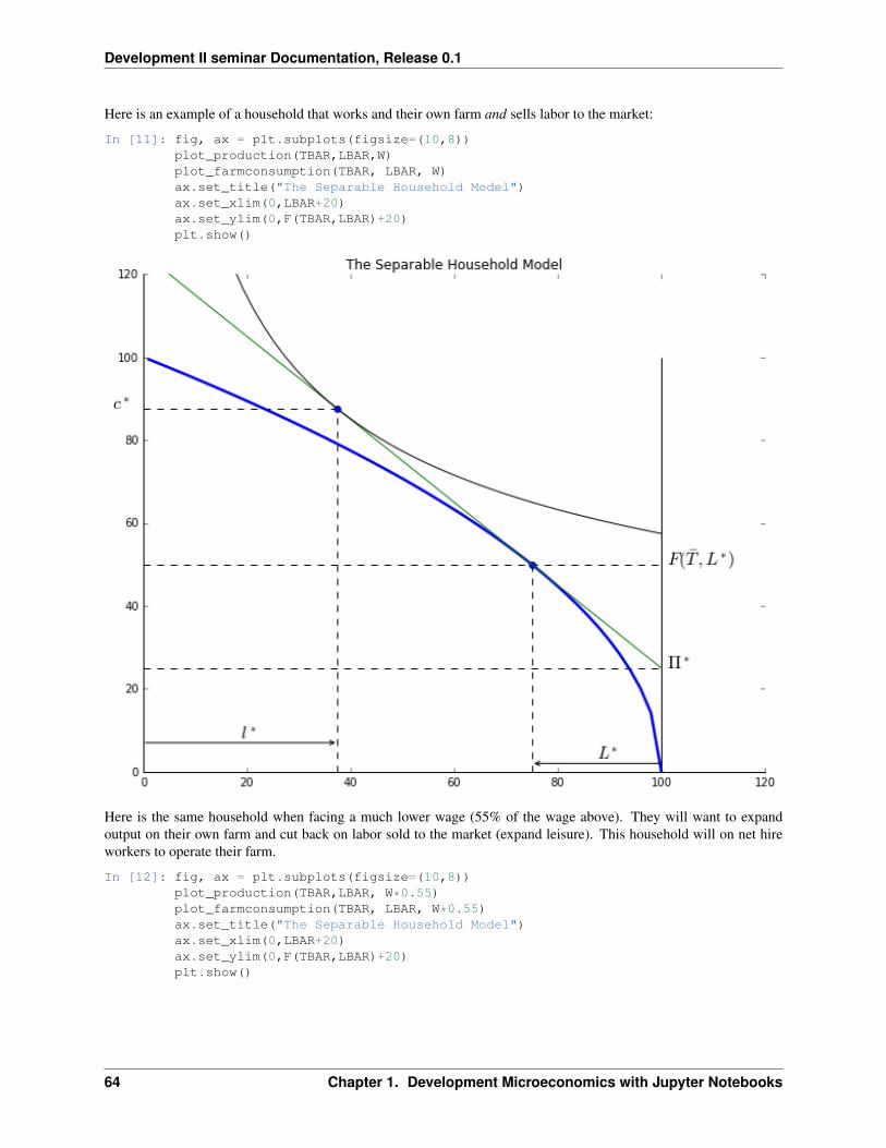
Development II seminar Documentation, Release 0.1
Here is an example of a household that works and their own farm and sells labor to the market:
In [11]: fig, ax = plt.subplots(figsize=(10,8))plot_production(TBAR,LBAR,W)plot_farmconsumption(TBAR, LBAR, W)ax.set_title("The Separable Household Model")ax.set_xlim(0,LBAR+20)ax.set_ylim(0,F(TBAR,LBAR)+20)plt.show()
Here is the same household when facing a much lower wage (55% of the wage above). They will want to expandoutput on their own farm and cut back on labor sold to the market (expand leisure). This household will on net hireworkers to operate their farm.
In [12]: fig, ax = plt.subplots(figsize=(10,8))plot_production(TBAR,LBAR, W*0.55)plot_farmconsumption(TBAR, LBAR, W*0.55)ax.set_title("The Separable Household Model")ax.set_xlim(0,LBAR+20)ax.set_ylim(0,F(TBAR,LBAR)+20)plt.show()
64 Chapter 1. Development Microeconomics with Jupyter Notebooks
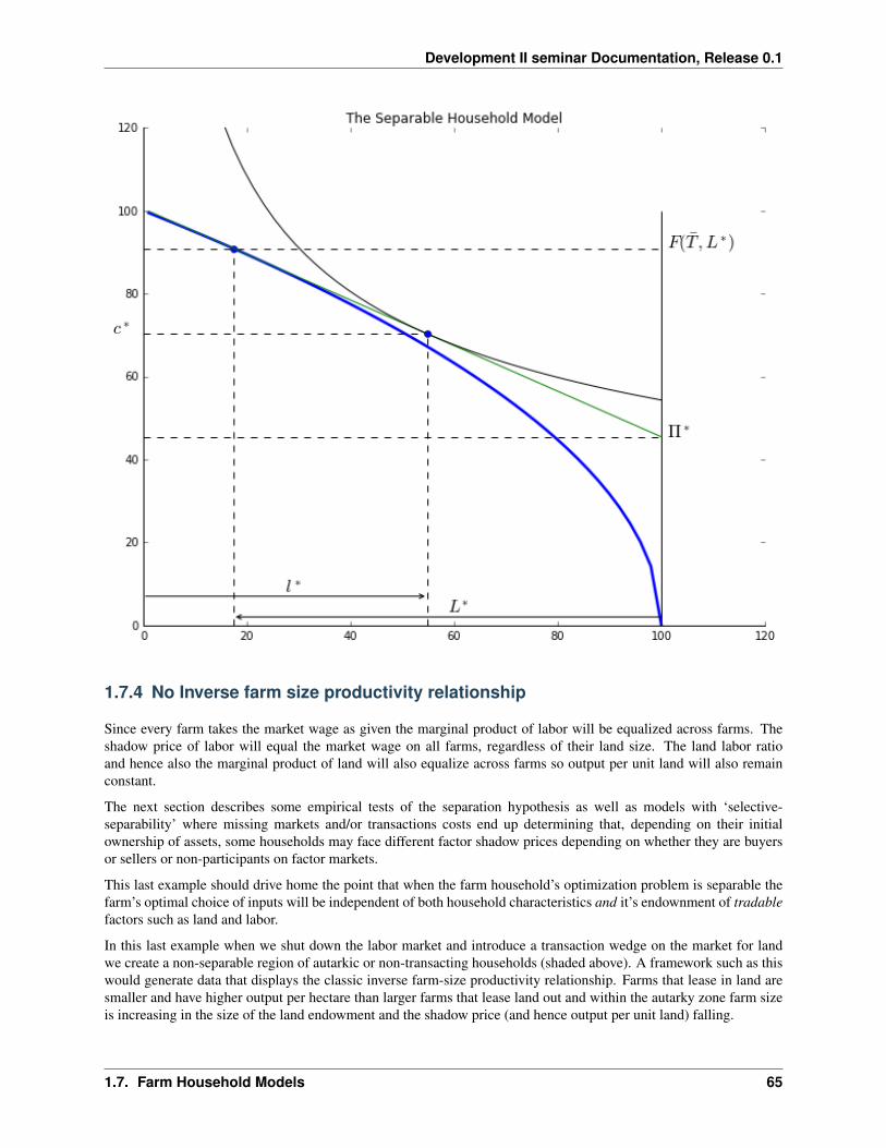
Development II seminar Documentation, Release 0.1
1.7.4 No Inverse farm size productivity relationship
Since every farm takes the market wage as given the marginal product of labor will be equalized across farms. Theshadow price of labor will equal the market wage on all farms, regardless of their land size. The land labor ratioand hence also the marginal product of land will also equalize across farms so output per unit land will also remainconstant.
The next section describes some empirical tests of the separation hypothesis as well as models with ‘selective-separability’ where missing markets and/or transactions costs end up determining that, depending on their initialownership of assets, some households may face different factor shadow prices depending on whether they are buyersor sellers or non-participants on factor markets.
This last example should drive home the point that when the farm household’s optimization problem is separable thefarm’s optimal choice of inputs will be independent of both household characteristics and it’s endownment of tradablefactors such as land and labor.
In this last example when we shut down the labor market and introduce a transaction wedge on the market for landwe create a non-separable region of autarkic or non-transacting households (shaded above). A framework such as thiswould generate data that displays the classic inverse farm-size productivity relationship. Farms that lease in land aresmaller and have higher output per hectare than larger farms that lease land out and within the autarky zone farm sizeis increasing in the size of the land endowment and the shadow price (and hence output per unit land) falling.
1.7. Farm Household Models 65
Development II seminar Documentation, Release 0.1
1.8 Testing for Separation in Household models
There are a few related approaches to testing for separation. The early studies were ‘global’ tests that aimed ataccepting or rejecting the null hypothesis of a separable household model for the entire sample of households. Somelater studies argue that a more typical situation is one where only ‘local’ subsets of households may be constrainedand therefore caught in a ‘non-separable’ regime and that any econometric estimation strategy should be sensitive tothis fact.
1.8.1 Global separation tests:
One approach attempts to test the implication of the separation hypothesis that labor demand should be independent ofhousehold preference shifters 𝐴 (i.e. demographic characteristics of the household. Basically this approach regresseslabor demand on prices, fixed non-traded inputs, and a measure of 𝐴. The null hypothesis is that the model is separableand the coefficient on A is zero. Therefore an insignificant estimated coefficient is interpreted as a failure to reject thenull hypothesis of separation. There are econometric issues such as simultaneity bias to worry about of couse. This isthe approach of papers such as Lopez (1984), Benjamin (1992) and many others.
Another approach builds from the observation that under separation the shadow price of labor or the marginal productof labor on the farm – call it 𝑤* – should equal the market wage 𝑤. Since the shadow wage is not directly observedit must be calculated off an estimated production function. If estimates of 𝑤* have been estimated across farms theseparation test boils down to a test of whether 𝛽0 = 0 and 𝛽1 = 1 in the regression 𝑤* = 𝛽0 + 𝛽1𝑤. Issues ofendogeneity and other econometic concerns must be addressed. This is the approach of Jacoby (1993), Skoufias(1994) and others.
Kien Le (2010) proposes a semi-parametric method that combines elements of both of the above approaches but usesless data. his apprach boils down to regressing the log of the measured value of output per worker on each farm againstthe market wage and a few controls.
1.8.2 Selective-separability
A small but important literature attempts to model farm household behavior on markets with transactions costs. Thebasic idea is that transactions costs such as the cost of getting to work can establish a wedge between the cost of hiringand selling labor. Suppose for example that farms that hire have to pay workers a wage of 𝑤 per hour but workerstake home only 𝑤(1 − 𝜏) of the wage due to transaction costs. If a would-be worker has the option of operating theirown farm it should be clear that they would work sell their labor to the market as long as the shadow price (marginalproduct) of labor on their own farm falls below 𝑤(1 − 𝜏), they will neither hire nor sell labor to the market if theshadow price of labor is above 𝑤(1 − 𝜏) but below 𝑤 and they will hire labor if the shadow price is above 𝑤. Ina simple model where other factors of production (say land or farming skill) are missing then households may beplaced into each of these three regimes (hiring out, self-sufficient, hiring in) depending on the initial distribution ofthese non-traded assets across households. The extent of allocative inefficiency (misallocation compared to the sameeconomy without transaction costs) will depend on both the size of the transaction costs and the initial distribution ofnon-traded assets. In the simple model I’ve just traced out households that operate farms and also hire out labor willin general be producing using more labor-intensive methods compare to households that hire-in labor since the latterface a higher wage.
de Janvry et al (1991) highlight some of the many ‘puzzles’ and behaviors that can be explained by adding transactioncosts to an otherwise neoclassical model. Sadoulet et al (1996) appear to be one of the earliest, if not the earliest paperto use the term ‘selective separability’ to refer to this fact that households may be selectively in one regime or another,depending on their asset holdings.
66 Chapter 1. Development Microeconomics with Jupyter Notebooks
Development II seminar Documentation, Release 0.1
Carter and Yao (2002): Local versus Global Separability
Carter and Yao’s (2002) paper “Local versus Global Separability in Agricultural Household Models: The factor priceequalizaiton effect fof land transfer rights,” offers an example of local versus global separability tests. They consider amodel where transaction costs establish a wedge between the rental rate tenants must pay to hire-in land and the rentalrate that landlords receive for hiring-out land. In a relatively simple model where the labor market is closed (whichthey argue fits their Chinese panel dataset from 1988 and 1993) this situation will generate a three regime equilibrium:(1) households with an endowment ratio of land relative to labor below some threshold will be tenants and hire-inland but these households are price-takers and the regime is separable in that all households in this group employ acommon high labor intensity and low shadow wage. (2) households with an endowment ratio above a different higherthreshold will rent-out land and are also in a separable regime but with a lower labor-land intensity and higher shadowwage. Finally households in the non-separable autarky regime (3) are those with endowment ratios between the twothresholds; these households do not hire in or hire out land but instead employ the land they have which means thatfor households in this group the shadow wage rises with the endowment ratio.
As the authors point out, referring to earlier ‘global’ tests:
. . . neither separability, nor non-separability exist globally across the full endowment continuum . . . thereduced form global separability tests found in the econometrics literature (which do not distinguish be-tween rental regimes) would be mis-specified and subject to a degree of bias that depends on the distribu-tion of households across the three regimes.
They employ a switching regression approach where the model of labor intensity to be estimated depends on thediscrete rental regime a household is classified into. The authors employ a simulated MLE method to estimate thesystem with panel data. They contrast their estimates with what would be found on the same dataset with one of theglobal tests of separability, arguing that the results from a global test are biased and misleading.
Carter and Yao’s (2002) paper “Local versus Global Separability in Agricultural Household Models: The Factor PriceEqualization Effect of Land Transfer Rights”
were analyzing households in rural China in the late 80s and 90s, a period of transition where land markets were beingslowly liberalized. The authors describe the situation as one where it was reasonable to assume no market for wagelabor and a limited market for land. They model this last idea as a wedge between the rental rate that is receivedby households that lease out land 𝑟𝑂 = 𝑟(1 − 𝑐𝑂(𝑀)) and the amount that households had to pay to rent land in𝑟𝐼 = 𝑟(1 + 𝑐𝐼(𝑀)), where 𝑟𝑂 ≤ 𝑟 ≤ 𝑟𝐼 .
To see this clearly, suppose households (HH) are otherwise identical to each other in all respects – including the size oftheir labor force, call it ��𝑒 – and only differ in terms of their endowment of land 𝑇𝑖. Households can then be classifiedas belonging to one of three behavioral regimes, depending the relative size of their land endowment.
, two where household behavior can be characterized as separable, and one w.
1. HH that rent-in land, :math:‘T_i in (0,T^I]‘: Households with a low endowment of land will lease in land atthe high rent-in market rate 𝑟𝐼 to operate a farm of size 𝑇 𝐼 .
2. HH in autarky, :math:‘T_i in (T_I,T^O]‘: Households with a land endowment withing these two thresholdswill operate their own land at shadow rate 𝑟0 < 𝑟* < 𝑟𝐼 .
3. HH that rent-out land, :math:‘T_i in [T_O,bar T]‘: Households with a high endowment of land will leaseout land at the low rent-out market rate 𝑟𝑂 and operate a farm of size 𝑇𝑂.
Leaving aside the issue of how the equilibrium rental rate is determined (discussed in other sections) suppose 𝑟𝐼 and𝑟𝑂 are given. Then Households in the first regime operate farms of size maximize farm profits
𝑝 · 𝐹𝑇 (𝑇 𝐼 , ��𝑒) = 𝑟𝐼
Households in the third regime operate farms of size maximize farm profits
𝑝 · 𝐹𝑇 (𝑇𝑂, ��𝑒) = 𝑟𝑂
1.8. Testing for Separation in Household models 67
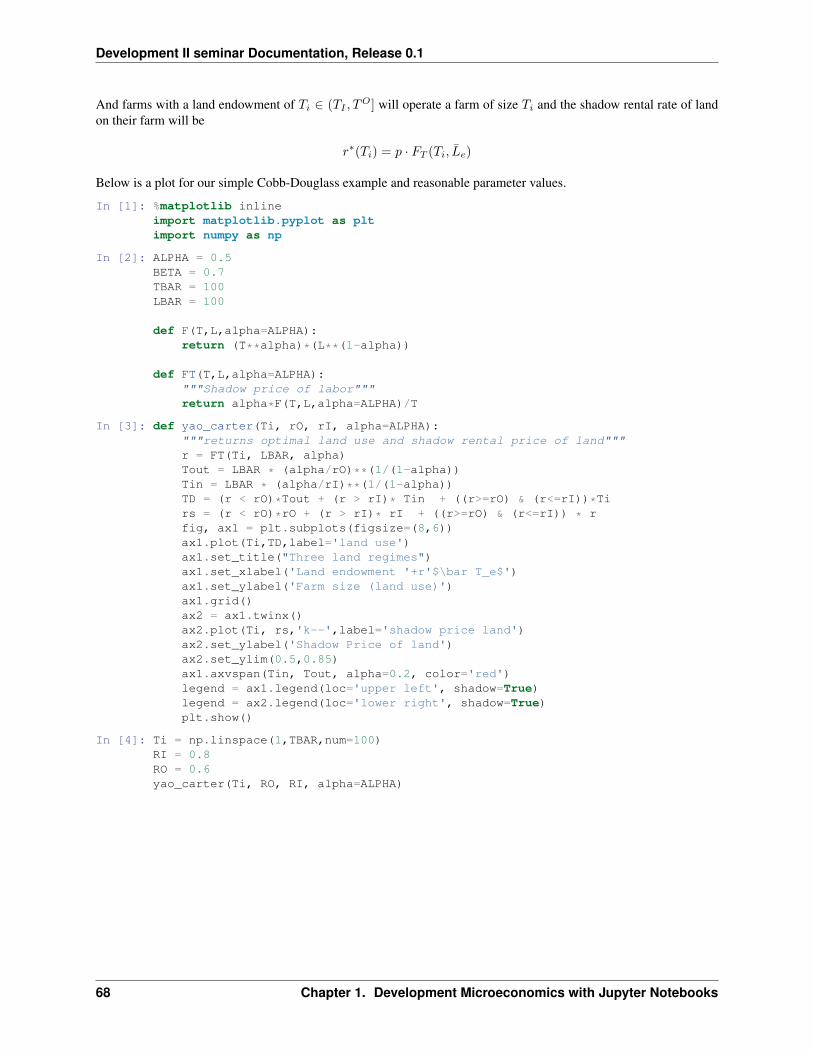
Development II seminar Documentation, Release 0.1
And farms with a land endowment of 𝑇𝑖 ∈ (𝑇𝐼 , 𝑇𝑂] will operate a farm of size 𝑇𝑖 and the shadow rental rate of land
on their farm will be
𝑟*(𝑇𝑖) = 𝑝 · 𝐹𝑇 (𝑇𝑖, ��𝑒)
Below is a plot for our simple Cobb-Douglass example and reasonable parameter values.
In [1]: %matplotlib inlineimport matplotlib.pyplot as pltimport numpy as np
In [2]: ALPHA = 0.5BETA = 0.7TBAR = 100LBAR = 100
def F(T,L,alpha=ALPHA):return (T**alpha)*(L**(1-alpha))
def FT(T,L,alpha=ALPHA):"""Shadow price of labor"""return alpha*F(T,L,alpha=ALPHA)/T
In [3]: def yao_carter(Ti, rO, rI, alpha=ALPHA):"""returns optimal land use and shadow rental price of land"""r = FT(Ti, LBAR, alpha)Tout = LBAR * (alpha/rO)**(1/(1-alpha))Tin = LBAR * (alpha/rI)**(1/(1-alpha))TD = (r < rO)*Tout + (r > rI)* Tin + ((r>=rO) & (r<=rI))*Tirs = (r < rO)*rO + (r > rI)* rI + ((r>=rO) & (r<=rI)) * rfig, ax1 = plt.subplots(figsize=(8,6))ax1.plot(Ti,TD,label='land use')ax1.set_title("Three land regimes")ax1.set_xlabel('Land endowment '+r'$\bar T_e$')ax1.set_ylabel('Farm size (land use)')ax1.grid()ax2 = ax1.twinx()ax2.plot(Ti, rs,'k--',label='shadow price land')ax2.set_ylabel('Shadow Price of land')ax2.set_ylim(0.5,0.85)ax1.axvspan(Tin, Tout, alpha=0.2, color='red')legend = ax1.legend(loc='upper left', shadow=True)legend = ax2.legend(loc='lower right', shadow=True)plt.show()
In [4]: Ti = np.linspace(1,TBAR,num=100)RI = 0.8RO = 0.6yao_carter(Ti, RO, RI, alpha=ALPHA)
68 Chapter 1. Development Microeconomics with Jupyter Notebooks
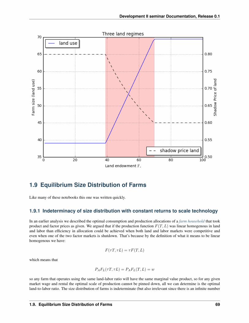
Development II seminar Documentation, Release 0.1
1.9 Equilibrium Size Distribution of Farms
Like many of these notebooks this one was written quickly.
1.9.1 Indeterminacy of size distribution with constant returns to scale technology
In an earlier analysis we described the optimal consumption and production allocations of a farm household that tookproduct and factor prices as given. We argued that if the production function 𝐹 (𝑇, 𝐿) was linear homogenous in landand labor than efficiency in allocation could be achieved when both land and labor markets were competitive andeven when one of the two factor markets is shutdown. That’s because by the definition of what it means to be linearhomogenous we have:
𝐹 (𝜏𝑇, 𝜏𝐿) = 𝜏𝐹 (𝑇, 𝐿)
which means that
𝑃𝐴𝐹𝐿(𝜏𝑇, 𝜏𝐿) = 𝑃𝐴𝐹𝐿(𝑇, 𝐿) = 𝑤
so any farm that operates using the same land-labor ratio will have the same marginal value product, so for any givenmarket wage and rental the optimal scale of production cannot be pinned down, all we can determine is the optimalland-to-labor ratio. The size distribution of farms is indeterminate (but also irrelevant since there is an infinite number
1.9. Equilibrium Size Distribution of Farms 69
Development II seminar Documentation, Release 0.1
of efficient ways to distribute the efficient output among farms that all have access to the same technology – and everyfarm makes zero profits).
If in a scenario like this we shut down the land market then the size distribution of farms becomes determined simplyby however much land each household has in its endowment. Efficiency in production allocation will still be achievedhowever if there is a competitive labor market as households hire in or hire out labor to bring the land to labor ratio toa level that efficiently equalizes marginal value products across farms.
1.9.2 Non-traded skills, diseconomies of scale and determinate size distribution
Suppose that we instead had a production function 𝐹 (𝑆, 𝑇, 𝐿) which is linear homogenous in its three arguments 𝑆, 𝑇 ,and 𝐿 where 𝑆 is refers to a non-traded farming skill or ability, 𝑇 is tradable land and 𝐿 is tradable labor. Considerfor example Cobb-Douglas function of the form:
𝐹 (𝑆, 𝑇, 𝐿) = 𝑆1−𝛾[𝑇𝛼𝐿1−𝛼
]𝛾where 𝛾 and 𝛼 are both numbers greater than 0 and less than or equal to 1. This production function is clearly linearhomogenous in its three arguments. Suppose now however that farming skill 𝑆 is non-traded and each household hadan endowmment of exactly 𝑆 = 1 units of farming skill. The conditional production
𝐹 (𝑇, 𝐿) = 𝐹 (𝑆 = 1, 𝑇, 𝐿)
𝐹 (𝑇, 𝐿) =[𝑇𝛼𝐿1−𝛼
]𝛾is clearly linear homogenous of degree 𝛾 and if 𝛾 is strictly less than one then it’s a production function subject todiseconomies of scale. In contrast to a productino function subject to constant returns to scale where the marginal costand average cost of production to a price taking firm are constant, when production is subject to diseconomies of scalethe firm’s marginal cost and average cost curves will both be upward sloping: as the firm doubles its inputs output lessthan doubles so average (and marginal) cost increases with output. This will then determine an optimal scale to thefirm (where marginal cost equals the market price of output).
Note also that if there are two firms that are otherwise identical but where one firm has a larger endowment of thenon-traded farming skill input, then it will be optimal for this more skilled farmer to operate at a larger scale. This canbe seen very simply by noting that the marginal product of labor and capital are both augmented by farming skill.
This then means that if there is some initial distribution of farming skill 𝑆 across households then the equilibrium sizedistribution of operational farm sizes will be in some way proportional to that distribution – farm households withhigher farming skills will operate larger farms that use both more land and labor. Since the production function ishomogenous in land and labor it’s also homothetic and though different farms will operate at different scale they willstill all operate using the same land-labor ratio in an efficient competitive allocation.
Lucas (1978) calls a model very similar to this a ‘span of control model. The basic idea is that because farm man-agement/supervision ability cannot be hired on the market due perhaps to moral hazard considerations. As a farmerattempts to use their fixed farming skill to supervise a larger and larger farm they face diseconomies of scale (𝐹𝑆𝑇 < 0and 𝐹𝑆𝐿 < 0) or rising costs. This will mean that a household that starts with a large endowment of land but onlymedium farming ability would find it optimal to operate a farm up to a certain scale and then lease out remaining landto the market (because the shadow return to employing land on a yet larger farm would fall below the land rental ratethey can get from the market.
Lucas’ (1978) ,pde; complicates things by assuming that the household has to choose between allocating its timeendowment between being a pure farm manager/supervisor or being a laborer. This then leads to a partition of house-holds: those above some threshold level of farming skill become full time farm operators who hire in labor and possiblyland all those below this threshold do not operate farms and derive income only from selling labor and possibly landto the market.
It turns out that simplifying Lucas’ model yields a richer model of the farm economy. In the model that follows everyhousehold has an endowment of farming skill, household labor and land, all of which will be supplied inelastically.
70 Chapter 1. Development Microeconomics with Jupyter Notebooks
Development II seminar Documentation, Release 0.1
Farming skill is independent of labor use, so the household is not forced to choose between farm supervision and workin the labor market, they can do both.
Competitive Factor Markets with no distortions
Let’s first study the benchmark cases where though there is no market for the non-traded farming skill, the othertwo factors land and labor can be costlessly hired in or out on competitive markets, resulting in competitive efficientequilibria.
Equal distribution of farming skill across households
Consider the simplest version of the model. Every household has access to the same Cobb Douglas production tech-nology, has 𝑆 = 1 units of farming skill and there is some distribution of the total endowment of land 𝑇 and labor ��across households. So tradable endowments (𝑇𝑖, ��𝑖) follow some distribution Γ.
To fix ideas suppose that there is an integer number of farm households ��. Since every farm household has the sametechnology and farming skill and face the same equilibrium market factor prices 𝑤 and 𝑣 they’ll choose the sameoptimal factor demands call them (𝑇𝐷(𝑤, 𝑟), 𝐿𝐷(𝑤, 𝑟)). Equilibrium in the factor markets requires:
��𝐿𝐷(𝑤, 𝑟) = ��
��𝑇𝐷(𝑤, 𝑟) = 𝑇
it follows that the optimal farm size will employ 𝐿* = 1 worker, 𝑇 * = 𝜏* = 𝑇��
units of land and will produce𝐹 (1, 𝜏*, 1) units of output. Equilibrium factor prices are also then simply determined as 𝑤* = 𝐹𝐿 (1, 𝜏*, 1) and𝑟* = 𝐹𝑇 (1, 𝜏*, 1). If the household has a land endowment 𝑇𝑖 larger than (less than) this optimal farm scale 𝜏* thehousehold leases out (leases in) land and likewise any household has a labor endowment ��𝑖 larger than (less than) thisoptimal farm scale 𝐿* hires out (hires in) labor.
Unequal distribution of farming skill across households
This simple model is easily adapted to the situation where households have access to the same technology but differ intheir initial level of farm management/supervision skill. Conceptually farmers with larger non-traded farming skill willoperate proportionately larger farms but the land-to-labor ratio is equalized across farms. It’s quite easy to demonstratethat if the initial distribution of skills is distributed as a log-normal then so too will the distribution of optimal farmsizes. Once again the farm household will lease out (lease in) land and hire out (hire in) labor depending on whethertheir initial holding of the traded land endowment exceeds (falls short of) the optimal land size for their farming skilland whether their initial holding of the traded labor endowment exceeds (falls short of) the optimal labor demand fortheir farming skill.
If we add in a fixed cost to operating a farm then farmers of very low skill will find it unprofitable to operate a farmand will become pure laborers and lease out all land.
Depending on the initial allocation of non-traded skills and tradable inputs households the model delivers an endoge-nous fourfold classification of the types of engagement in this farm labor economy (the labels I use here are similarto Eswaran and Kotwal’s (1986) paper): * pure laborers: low skill households do not operate farms. * laborer-cultivators: low-medium skill households operate small farms and also seek outside employment * capitalist: higherskill households operate larger farms with hired labor.
In the economy described thus far, farm household decisions are separable and the initial distribution of tradable landand labor does not matter for efficiency in production.
Note that because our production function was linear homogenous in the three inputs we could shut down one of themarkets – the market for farming skill – and still achieve efficiency in production.
1.9. Equilibrium Size Distribution of Farms 71
Development II seminar Documentation, Release 0.1
We can think of the Eswaran and Kotwal (1986) model in these terms. They describe a model with land, labor andlabor supervision. We’ve shut down the market for supervisory labor whereas they tell a more complicated story aboutmoral hazard which at the end of the day introduces a similar type of diminishing returns to supervision. That marketimperfection by itself is not enough to matter for efficiency in allocation but they then go ahead and introduce a seconddistortion: they impose the requirement that farms must pay for their land and labor hiring in advance of the crop butthen make a farm household’s access to capital proportional to it’s initial holding of land (they also impose a fixed costof operation similar to that described above).
The working capital constraint means that some farms will not be able to achieve their optimum scale of operation andthe initial distribution of land will now determine both efficiency in allocation and the endogenous agrarian structure:the proportion of different types of farm operators in the economy.
Let’s see a simple simulation of this model after a brief note on the code we will use to solve for equilibria.
A note on python implementation and object-oriented programming
Most of the code to run the model below is contained in a separate module geqfarm.py outside of this notebook thatwill be imported as any other library.
It’s often said that in python ‘everything is an object.’ Objects have attributes and methods. ‘Attributes’ can be thoughtof as data or variables that describe the object and ‘methods’ can be thought of as functions that operate on object.
Take a very simple example. When in python you declare a string variable like so:
In [29]: mystring = 'economics'
python treats mystring as an instance of a string object. One then has access to a long list of attributes and methodsassociated with this object. In a jupyter notebook if you type the variable name mystring followed by a period andthen hit the tab key you will see a list of available attributes and methods. Here are a few:
In [30]: # return the string capitalizedmystring.upper()
Out[30]: 'ECONOMICS'
In [31]: # count the number of occurunces of the letter 'o'mystring.count('o')
Out[31]: 2
In [32]: # tell me if the string ends with the letter 'M'mystring.endswith('M')
Out[32]: False
Class statements to create new objects
Let’s import the geqfarm.py libary:
In [33]: import numpy as np
In [34]: from geqfarm import *
If you take a look at the code you will see how I have used class statements to create a new prototype ‘Economyobject. An object of type Economy has attributes such as the number of households in the economy, parameters of theproduction function, and arrays that summarize the initial distribution of skill, land and labor across households. Oncethis class of object is defined one can make assignments such as the following:
In [35]: myeconomy= Economy(20)
This creates myeconomy as an instance of an Economy object. Several attributes are set to default values. We caneasily find out what these are. For instance this is an economy with a production function with the 𝛾 paramter whichmeasures the extent of homogeneity or diseconomies of scale. To find out what value it’s set to we just type:
72 Chapter 1. Development Microeconomics with Jupyter Notebooks
Development II seminar Documentation, Release 0.1
In [36]: myeconomy.GAMMA
Out[36]: 0.8
And we can easily change it to another value:
In [37]: myeconomy.GAMMA = 0.9
I’ve written a method to get a convenient summary of all important parameters:
In [38]: myeconomy.print_params()
ALPHA : 0.5 GAMMA : 0.9 H : 0.0 LAMBDA : 0.05LBAR : 100 N : 20 TBAR : 100 s : [ 1. 1. 1. 1. 1. 1. 1. 1. 1. 1. 1. 1. 1. 1. 1. 1. 1. 1.
1. 1.]
For example, the number of households is 𝑁 = 20, total land endowment and labor force are both set to 100 and 𝑠 isan array of skills across each of those 20 households. For the moment every household has the same skill level.
Let’s work with a different simpler economy of just 𝑁 = 5 identical households. We’ll call this new economy just E.
In [39]: N = 5E = Economy(N)E.ALPHA = 0.5E.GAMMA = 0.90
I’ve written a simple object method which calculates a competitive equilibrium allocation for the economy. I’ve set itup to take as required inputs a vector of economywide endownments and an array summarizing the skill distribution.It returns a ‘named-tuple’ with the vector of equilibrium factor prices, and the optimal land and labor allocations oneach farm.
In [40]: eqnE = E.smallhold_eq([E.TBAR, E.LBAR], E.s)
The competitive equilibrium land rent and labor wage that clears this market are given by:
In [41]: eqnE.w
Out[41]: array([ 0.3335, 0.3335])
The optimal allocation of land and labor to each of the five farm skill groups is given by:
In [42]: eqnE.X
Out[42]: array([[ 20., 20., 20., 20., 20.],[ 20., 20., 20., 20., 20.]])
Since every one of the 5 farm household has the same skill and there are 100 units of land and labor the optimalallocation is for every farm to operate with 20 units of land and 20 units of labor.
Suppose however we now increase the skill of only the very first household, household zero.
In [43]: E.s[0] = 1.2E.s
Out[43]: array([ 1.2, 1. , 1. , 1. , 1. ])
Let’s recalculate the competive equilibrium:
In [44]: eqnE = E.smallhold_eq([E.TBAR, E.LBAR], E.s)
Since there is more skill in this economy we would expect real wages and rents to rise, as indeed they do:
In [45]: eqnE.w
Out[45]: array([ 0.3581, 0.3581])
Since farm household zero now has a considerably higher level of skill compare to other households it’s optimal scaleof operations increases and, since it bids on the market for the same factors driving up the costs to other farms, theoptimal scal of operations of the other farms shrinks.
1.9. Equilibrium Size Distribution of Farms 73
Development II seminar Documentation, Release 0.1
In [46]: eqnE.X
Out[46]: array([[ 60.7525, 9.8119, 9.8119, 9.8119, 9.8119],[ 60.7525, 9.8119, 9.8119, 9.8119, 9.8119]])
Equilibria with credit market distortions
We can easily modify to model above to get a simplified version of the model used in Eswaran and Kotwal’s 1996Economic Journal paper “Access to Capital and Agrarian Production Organization.”
The model is as above except that now we add in a farm-specific working capital constraint, or the requirement thatfarms must be able to hire their inputs up-front prior to sale of their crop.
1.9.3 Latifundia Economics: factor market-power distortions
In [47]: %load_ext autoreload%autoreload 2
The autoreload extension is already loaded. To reload it, use:%reload_ext autoreload
In [48]: import numpy as npfrom matplotlib import pyplot as pltplt.rcParams["figure.figsize"] = (10, 8)
np.set_printoptions(precision=4)%matplotlib inline
What follows is a simple description of my (2007) ‘Latifundia Economics’ paper, which I used to try to explain theLatifundia-Minifundia complex of bimodal distribution of farm sizes that existed for long periods of time in manyparts of historical Latin America and other parts of the world.
To understand the main arguments, consider the simplest case of a single landlord (or a cartel of landlords) surroundedby a fringe of small landowning or landless agricultural households. If the lanlord owns a large fraction of the landendowment a standard partial-equilibrium analysis of non-price discriminating monopoly suggests the landlord woulddrive up the rental price of land by withholding land from the lease market. In a general equilibrium setting howeverthere is another effect: by restricting other farmers’ access to land landlords also lower the marginal product of laboron those farms. This increases the supply of labor to landlord estates at any given wage increasing landlords’ potentialincome from monopsony rents. This can lead to equilibria where landlords increase the size of their production estatesscale well above efficient scale in a competitive economy. A Latifundia-Minifundia type economy can emerge inwhich landlords operate large estates employing overly land-intensive production techniques while a large mass offarmers operate inefficiently and labor-intensive small parcels of land and sell labor to the landlord estate(s).
Let’s start with a simplified statement of the problem with just two types of households – landlords and ‘peasants’ anda very simple discrete distribution of farming skills. We’ll later extend this to a much more general setting.
The economy has 𝑇 units of cultivable land and 𝐿 households with one unit of labor each. The economy-wide land tolabor ratio is therefore 𝑡 = 𝑇/𝐿.
Household are indexed 𝑖 = 1.. 𝐿 and each household has a non-traded farming skill level 𝑠𝑖 drawn from aknown distribution 𝑍. There is also an initial distribution of property rights over land. We’ll make moreflexible assumptions later but for now suffice to say that there is a group of “landlord” households (fraction $𝜆$𝑜𝑓𝑡ℎ𝑒𝑡𝑜𝑡𝑎𝑙)𝑤ℎ𝑜𝑡𝑜𝑔𝑒𝑡ℎ𝑒𝑟𝑜𝑤𝑛𝑓𝑟𝑎𝑐𝑡𝑖𝑜𝑛$𝜃$𝑜𝑓𝑡ℎ𝑒𝑙𝑎𝑛𝑑𝑒𝑛𝑑𝑜𝑤𝑚𝑒𝑛𝑡.𝐼𝑛𝑠𝑜𝑚𝑒𝑠𝑐𝑒𝑛𝑎𝑟𝑖𝑜𝑠𝑏𝑒𝑙𝑜𝑤𝑡ℎ𝑒𝑦𝑤𝑖𝑙𝑙𝑐𝑜𝑙𝑙𝑢𝑑𝑒𝑡𝑜𝑐𝑜𝑜𝑟𝑑𝑖𝑛𝑎𝑡𝑒𝑡ℎ𝑒𝑖𝑟𝑓𝑎𝑐𝑡𝑜𝑟𝑚𝑎𝑟𝑘𝑒𝑡𝑑𝑒𝑚𝑎𝑛𝑑𝑠𝑎𝑛𝑑𝑠𝑢𝑝𝑝𝑙𝑖𝑒𝑠𝑎𝑠𝑖𝑓𝑡ℎ𝑒𝑦𝑤𝑒𝑟𝑒𝑎𝑠𝑖𝑛𝑔𝑙𝑒𝑙𝑎𝑛𝑑𝑙𝑜𝑟𝑑‘𝑐𝑎𝑟𝑡𝑒𝑙′.
As the 𝜆𝐿 landlord households own 𝜃𝑇 units of land, peasant households own the remaining (1 − 𝜃)𝑇 units. Theaverage non-landlord household therefore owns (1−𝜃)𝑡
(1−𝜆) units and, for the moment, all peasant households have thesame initial land endowment. Under these assumptions it can be shown that the land Gini coefficient is exactly[𝜃 − 𝜆] .
74 Chapter 1. Development Microeconomics with Jupyter Notebooks
Development II seminar Documentation, Release 0.1
A single tradable good such as corn is produced and consumed in the economy at a unity price fixed by trade with theworld market. Households maximize utility from consumption subject to household income from farm productionplus net factor sales.
All peasant households have access to the same production technology represented by a standard concave productionfunction 𝐹 (𝑇, 𝐿, 𝑠) assumed for now to be linearly homogenous in its three arguments: land 𝑇,labor 𝐿, and a thirdfactor which we label 𝑠.This last factor is assumed to be a non-traded factor that captures farming skill or laborsupervision ability.
In the illustrative simulations below we assume a Cobb-Douglas form
𝐹 (𝑇, 𝐿, 𝑠) = 𝑠1−𝛾 ·[𝑇𝛼𝐿1−𝛼
]𝛾Latifundia Economics (factor market power distorted equilibria)
The following contrived example helps to starkly highlight the mechanisms behind the factor-market power distortedequilibrium.
TO start simple assume that there just N=5 farmers each with a skill level normalized to 1.
In [49]: N = 5
Now create an economy and change a few parameters from their default. The 𝛾 parameter which measures the degreeof homogeneity in production is purposefully set very high.. We are very close to assuming constant returns to scale(but setting it just below 1 is needed to make sure the size-distribution remains determinate).
In [50]: E = Economy(N) # an instance takes N length as parameters = np.ones(N) # skill distribution in the economyE.ALPHA = 0.5E.GAMMA = 0.90
The Economy has default resource endowment:
In [51]: E.TBAR,E.LBAR
Out[51]: (100, 100)
So as expected the efficient (competitive) resource allocation has every farmer operating a farm of equal unit size. Thesmallhold_eq method gives the competitive (efficient) allocation for a subeconomy with XE = (TE,LE) endowmentsand skill distribution s. It returns a named tuple with equilibrium facor prices and X=[T,L] allocations.
If XE and s are those of the entire economy then we’ve found the economywide competitive allocation.
In [52]: Xc = E.smallhold_eq([E.TBAR,E.LBAR],s)Xc
Out[52]: result(w=array([ 0.3335, 0.3335]), X=array([[ 20., 20., 20., 20., 20.],[ 20., 20., 20., 20., 20.]]))
In [53]: (Xrc,Xr,wc,wr) = scene_print(E,10, detail=True)
Running 10 scenarios...
Assumed Parameters==================ALPHA : 0.5 GAMMA : 0.9 H : 0.0 LAMBDA : 0.2LBAR : 100 N : 5 TBAR : 100 s : [ 1. 1. 1. 1. 1.]
Effcient:[ Trc, Lrc] [rc,wc] w/r F( ) [r*Tr] [w*Lr]==============================================================================
[ 20.00, 20.00] [0.33,0.33] 1.00 | 14.82 6.67 6.67
Theta [ Tr, Lr ] [rM,wM] w/r | F() [T_hire] [T_sale] [L_hire]
1.9. Equilibrium Size Distribution of Farms 75
Development II seminar Documentation, Release 0.1
==============================================================================0.00 [ 17.56, 20.69] [ 0.33, 0.34] 1.04 | 14.19 5.74 0.00 7.030.10 [ 18.57, 20.17] [ 0.33, 0.34] 1.02 | 14.39 6.13 3.30 6.790.20 [ 20.00, 20.00] [ 0.33, 0.33] 1.00 | 14.82 6.67 6.67 6.670.30 [ 21.95, 20.19] [ 0.34, 0.33] 0.98 | 15.52 7.41 10.13 6.670.40 [ 24.58, 20.78] [ 0.34, 0.33] 0.95 | 16.55 8.43 13.72 6.790.50 [ 28.15, 21.88] [ 0.35, 0.32] 0.92 | 18.00 9.85 17.50 7.040.60 [ 33.08, 23.67] [ 0.36, 0.32] 0.88 | 20.05 11.92 21.61 7.470.70 [ 40.17, 26.55] [ 0.38, 0.31] 0.81 | 23.05 15.13 26.36 8.140.80 [ 51.31, 31.70] [ 0.41, 0.29] 0.71 | 27.87 20.94 32.65 9.220.90 [ 74.78, 46.29] [ 0.53, 0.25] 0.47 | 39.14 39.33 47.34 11.430.99 [ 99.90, 94.35] [ 4, 0.07] 0.02 | 61.44 401.03 397.42 6.65
==============================================================================
Thus far we’ve said nothing of the ownership of land or labor. Let’s assume every household has one unit of labor butthat the ‘landlord’ class (which WLOG we index to be the last skill group s[-1]) owns fraction 𝜃 of the land. Assuminga uniform distribution of households across skills every skill group has Lbar/N households, and so there are that manylandlords who act as a single cartel.
The following code is useful for printing and plotting out equilibria as a function of initial landlords’ land ownershipshare.
We pass our economy instance to the scenarios function and it solves for competitive and market-power equilibria (atdifferent levels of theta) and prints out the results.
Let’s plot the results.. THis is the classic diagram from Latifundia Economics..
In [54]: factor_plot(E,Xrc,Xr)
76 Chapter 1. Development Microeconomics with Jupyter Notebooks
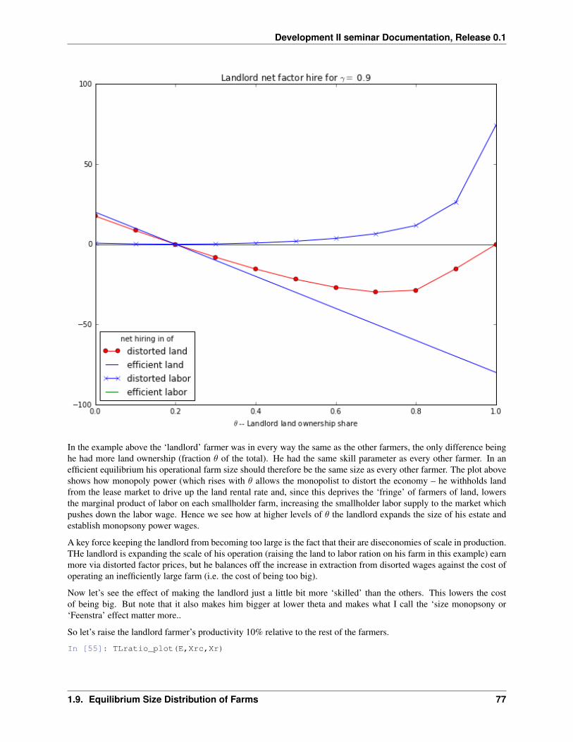
Development II seminar Documentation, Release 0.1
In the example above the ‘landlord’ farmer was in every way the same as the other farmers, the only difference beinghe had more land ownership (fraction 𝜃 of the total). He had the same skill parameter as every other farmer. In anefficient equilibrium his operational farm size should therefore be the same size as every other farmer. The plot aboveshows how monopoly power (which rises with 𝜃 allows the monopolist to distort the economy – he withholds landfrom the lease market to drive up the land rental rate and, since this deprives the ‘fringe’ of farmers of land, lowersthe marginal product of labor on each smallholder farm, increasing the smallholder labor supply to the market whichpushes down the labor wage. Hence we see how at higher levels of 𝜃 the landlord expands the size of his estate andestablish monopsony power wages.
A key force keeping the landlord from becoming too large is the fact that their are diseconomies of scale in production.THe landlord is expanding the scale of his operation (raising the land to labor ration on his farm in this example) earnmore via distorted factor prices, but he balances off the increase in extraction from disorted wages against the cost ofoperating an inefficiently large farm (i.e. the cost of being too big).
Now let’s see the effect of making the landlord just a little bit more ‘skilled’ than the others. This lowers the costof being big. But note that it also makes him bigger at lower theta and makes what I call the ‘size monopsony or‘Feenstra’ effect matter more..
So let’s raise the landlord farmer’s productivity 10% relative to the rest of the farmers.
In [55]: TLratio_plot(E,Xrc,Xr)
1.9. Equilibrium Size Distribution of Farms 77
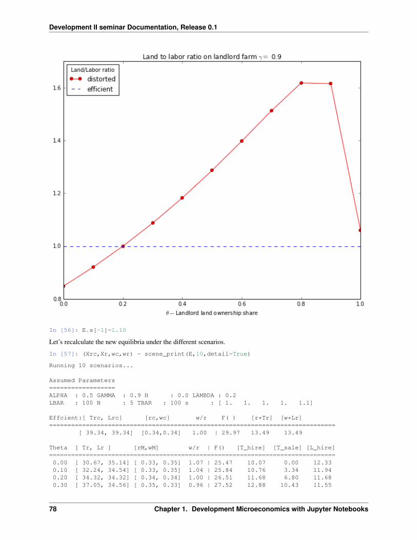
Development II seminar Documentation, Release 0.1
In [56]: E.s[-1]=1.10
Let’s recalculate the new equilibria under the different scenarios.
In [57]: (Xrc,Xr,wc,wr) = scene_print(E,10,detail=True)
Running 10 scenarios...
Assumed Parameters==================ALPHA : 0.5 GAMMA : 0.9 H : 0.0 LAMBDA : 0.2LBAR : 100 N : 5 TBAR : 100 s : [ 1. 1. 1. 1. 1.1]
Effcient:[ Trc, Lrc] [rc,wc] w/r F( ) [r*Tr] [w*Lr]==============================================================================
[ 39.34, 39.34] [0.34,0.34] 1.00 | 29.97 13.49 13.49
Theta [ Tr, Lr ] [rM,wM] w/r | F() [T_hire] [T_sale] [L_hire]==============================================================================0.00 [ 30.67, 35.14] [ 0.33, 0.35] 1.07 | 25.47 10.07 0.00 12.330.10 [ 32.24, 34.54] [ 0.33, 0.35] 1.04 | 25.84 10.76 3.34 11.940.20 [ 34.32, 34.32] [ 0.34, 0.34] 1.00 | 26.51 11.68 6.80 11.680.30 [ 37.05, 34.56] [ 0.35, 0.33] 0.96 | 27.52 12.88 10.43 11.55
78 Chapter 1. Development Microeconomics with Jupyter Notebooks
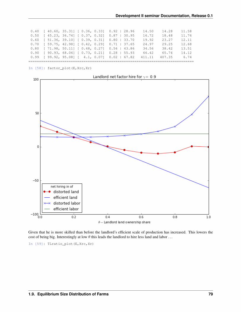
Development II seminar Documentation, Release 0.1
0.40 [ 40.60, 35.31] [ 0.36, 0.33] 0.92 | 28.96 14.50 14.28 11.580.50 [ 45.23, 36.74] [ 0.37, 0.32] 0.87 | 30.95 16.72 18.48 11.760.60 [ 51.36, 39.10] [ 0.39, 0.31] 0.80 | 33.70 19.92 23.27 12.110.70 [ 59.75, 42.98] [ 0.42, 0.29] 0.71 | 37.65 24.97 29.25 12.680.80 [ 71.98, 50.11] [ 0.48, 0.27] 0.56 | 43.86 34.56 38.42 13.510.90 [ 90.93, 68.06] [ 0.73, 0.21] 0.28 | 55.93 66.42 65.74 14.120.99 [ 99.92, 95.08] [ 4.1, 0.07] 0.02 | 67.82 411.11 407.35 6.74
==============================================================================
In [58]: factor_plot(E,Xrc,Xr)
Given that he is more skilled than before the landlord’s efficient scale of production has increased. This lowers thecost of being big. Interestingly at low 𝜃 this leads the landlord to hire less land and labor . . .
In [59]: TLratio_plot(E,Xrc,Xr)
1.9. Equilibrium Size Distribution of Farms 79
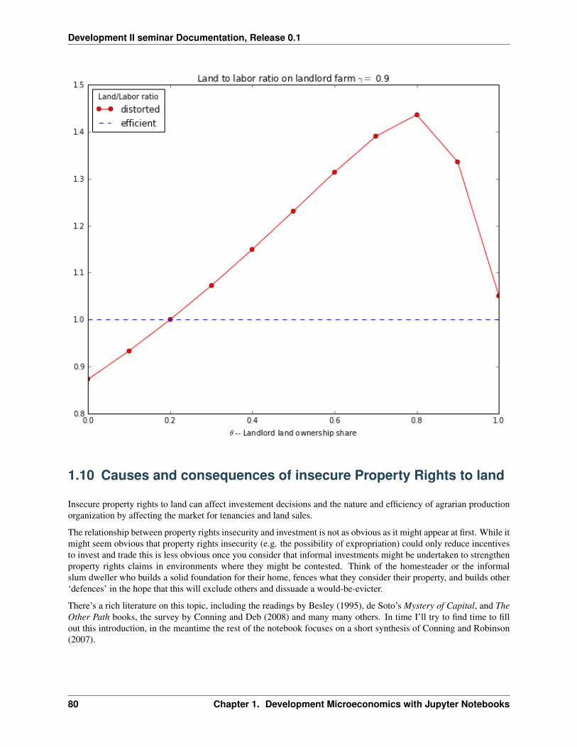
Development II seminar Documentation, Release 0.1
1.10 Causes and consequences of insecure Property Rights to land
Insecure property rights to land can affect investement decisions and the nature and efficiency of agrarian productionorganization by affecting the market for tenancies and land sales.
The relationship between property rights insecurity and investment is not as obvious as it might appear at first. While itmight seem obvious that property rights insecurity (e.g. the possibility of expropriation) could only reduce incentivesto invest and trade this is less obvious once you consider that informal investments might be undertaken to strengthenproperty rights claims in environments where they might be contested. Think of the homesteader or the informalslum dweller who builds a solid foundation for their home, fences what they consider their property, and builds other‘defences’ in the hope that this will exclude others and dissuade a would-be-evicter.
There’s a rich literature on this topic, including the readings by Besley (1995), de Soto’s Mystery of Capital, and TheOther Path books, the survey by Conning and Deb (2008) and many many others. In time I’ll try to find time to fillout this introduction, in the meantime the rest of the notebook focuses on a short synthesis of Conning and Robinson(2007).
80 Chapter 1. Development Microeconomics with Jupyter Notebooks
Development II seminar Documentation, Release 0.1
1.10.1 Conning & Robinson (2007): Property Rights and the Political Organizationof Agriculture
This is a simplified version of Conning and Robinson’s 2007 paper in the Journal of Development Economics, a“general equilibrium model where the organization of agriculture and the political equilibrium determining the securityof property rights are jointly determined.
In its present form this notebook focuses primarily on the economic side of the model which demonstrates howinsecure property rights to land (e.g. the risk of expropriation) might affect the equilibrium level of land leasing andequilibrium factor prices. The dull details of the probabilistic voting model that determines the equilibrium politicalrisk of expropriation are left for another time.
The model is another in the family of general equilibrium models of the size distribution of farms that we’ve alreadyanalyzed. In all cases we have an economy with an agricultural technology that is linear homogenous in farming skill𝑆, land 𝑇 and labor 𝐿. We showed that even though there was no market for farm management skills (so 𝑆 is anon-traded asset) efficient resource allocations could be achieved if we had competitive land and labor markets thatallowed households to achieve their efficient scale. This model is similar to Lucas’ 1978 size distribution of businessfirms and would explain the size distribution of farms as determined by an underlying distribution of farming skillsacross households. In this model efficiency of allocation is independent of the initial distribution of factors 𝑆, 𝑇, and𝐿 in the population.
If, in addition to the imperfection in the market for non-traded farming skills, we add a distortion to either the marketfor land or labor, efficiency can no longer be achieved.
Eswaran and Kotwal 1996 paper on “Access to Capital and Production Organization” can be viewed as a variant onthis type of benchmark model. They introduce two simultaneous distortions. They require that supervisory labor beused at increasing cost to supervise any hired labor. This is loosely analogous to our shutting down the market forfarming skill (or supervision) ability. The second constraint is a distortion in the market for working capital whichdetermines that households with low initial wealth (principally ownership of land) will be constrained in the marketfor working capital (in our benchmark model we implicitly assumed working capital could always be financed). Theinteraction of these two types of distortion determines that allocations cannot be efficient and also the shape of theequilibrium agrarian ‘class structure’ or occupational choice hiearchy). Even though in effect all farms have the samefarming skill, households with less ownership of land are more likely to be constrained in access to working capital andhence have to drop out of production entirely (to become ‘pure laborers’) or may be a constrained ‘labor-cultivator’who runs a small farm and then sells labor on the market. In addition households may be constrained or unconstrained‘capitalist’ farms that hire other workers.
Conning and Robinson’s paper sets itself up against a similar benchmark model, but in a two period world. In aworld with complete security of property rights land and labor markets will allocate land efficiently across farms inagriculture and labor efficiently across farms in agriculture and manufacturing activities in urban areas. The sizedistribution of farms in agriculture will be efficient and completely determined by the initial distribution of non-tradedfarming skills. Land tenancy markets will be efficient and active. Take the case of all households having the samefarming skill. If landlords have relatively large amounts of land they will lease it out to tenants to bring the distributionof operational farm sizes in line with the distribution of farming skills.
Starting with this benchmark the model asks what would happen if we introduce property rights insecurity in the formof the possibility of a ‘land to the tiller’ land or tenancy reform.
The Model with secure property rights
To simplify greatly assume there are just two population groups: landlords and peasant households. They have accessto the follwowing production technologies:
Peasants: 𝐹 (𝑇, 𝐿) Landlords:𝐺(𝑇, 𝐿) = 𝐴𝑙𝐹 (𝑇, 𝐿)
When 𝐴𝑙 = 1 landlord and peasant production technologies are identical, when 𝐴𝑙 > 1 landlords are more skilledfarmers and we associate that with higher productivity of labor and capital. For the moment assume 𝐴𝑙 = 1.
1.10. Causes and consequences of insecure Property Rights to land 81
Development II seminar Documentation, Release 0.1
Landlord and peasant housholds are each endowed with 1 unit of labor. There are �� households overall of whichproportion 𝑛𝑝 are peasant households and proportion 𝑛𝑙 are landlord households. For example if �� = 100 and𝑛𝑝 = 0.90 there would be 90 peasant households and 10 landlord households.
We will assume there is an urban sector where production takes place using production function 𝐻(𝐿) which is subjectto decreasing returns. In equilibrium 𝐿𝑢 units of labor will leave agriculture to work in the city.
The only difference between landlord and peasant households then is their ownership of land. Landlords as a groupown fraction 𝜃 of the overall land endowment. That means that each landlord household owns
𝜃
𝑛𝑙𝑡
units of land where 𝑡 = 𝑇��
Since by definition landlords own more land then peasants 𝜃 > 𝑛𝑙
In a world of secure property rights the first period allocations will be identical to the second period allocations, andin any given period efficient allocation will be characterized by:
𝑤 = 𝐹𝐿(𝑇𝑝, 𝐿𝑝) = 𝐺𝐿(𝑇𝑙, 𝐿𝑙) = 𝐻(𝐿𝑢)
𝑟 = 𝐹𝑇 (𝑇𝑝, 𝐿𝑝) = 𝐺𝑇 (𝑇𝑙, 𝐿𝑙)
In the special case where landlord and peasant farming skill is identical efficient production allocations will be identicalon all �� farms and equal to
𝑇 𝑒 =𝑇
��
𝐿𝑒 =��− 𝐿𝑒
𝑢
��
where 𝐿𝑒𝑢 is pinned down by 𝐹𝐿(𝑇 𝑒, 𝐿𝑒) = 𝑤 = 𝐻𝐿(𝐿𝑒
𝑢).
It’s easy to show the efficient share of cultivated land under tenancy should be
𝜏𝑒 = 𝜃 − 𝑛𝑙
Intuitively, the higher the concentration of land 𝜃 the more land needs to be under tenancy to equalize farm sizes.
The Model with insecure property rights
We now extend the setting to allow the initial production period to be followed by a political contest that will decidethe likelihood of future property rights reforms that may affect ownership claims in a final production period.
Households will choose factors of production as before except that there is now the threat that a tenancy reform mayoccur with (possibly zero) probability 𝛼.
If a reform takes place all sitting tenants obtain protection from eviction on fraction (1-𝜅) of the land they leased in thepre-reform period and they will only have to pay a new capped rental rate v for those leases in the following period,where v will generally be set at or below the post-reform market equilibrium rental rate 𝑣𝑒
One interpretation of 𝜅 is that the reform beneficiary might have to pay monetary expenses (𝑣𝑒 − 𝑣) per unit landtransferred to cover such things as property registration paperwork, new taxes, excess loan financing costs, or othertransaction or setup costs. The value of 𝜅 will be a key parameter establishing the size of the gap between the value ofproperty rights lost by the landlord and the value of benefits transferred to the tenant or squatter.
In a post-reform competitive equilibrium this transaction cost will be reflected in land rent and sale prices and how itsburden is shared between landlord and tenant it would not matter if we had instead imposed these transaction costsdirectly on the landlord.
82 Chapter 1. Development Microeconomics with Jupyter Notebooks
Development II seminar Documentation, Release 0.1
To simplify matters it is assumed that no further alteration of property rights can take place after the reform. Thisimplies that in the post-reform production period efficient resource allocation (𝑇𝑒, 𝐿𝑒, 𝐿𝑢𝑒) will be achieved at marketfactor prices 𝑣𝑒 = 𝐹𝑇 (𝑇𝑒, 𝐿𝑒) and 𝑤𝑒 = 𝐹𝐿(𝑇𝑒, 𝐿𝑒), except of course that reform beneficiaries now earn additionalincomes generated by the transfer of property rights.
We can model agrarian reforms of different type and depth by varying the three parameters , 𝑣 and . For example, onemay think of 𝑣 = 0 as expropriation without compensation to the landlord while 0 < 𝑣 < 𝑣𝑒 could be thought of asa tenancy reform with a rent ceiling, or as a land reform with partial compensation. From a landlord’s perspective aproperty rights reform means facing the prospect of being forced to cede the (𝑡/𝑛𝑙 − 𝑇𝑙) units of land they put underlease in the pre-reform phase at below-market rental rate v in the post-reform period.
Anticipating this the landlord will now choose 𝐿𝑙 and 𝑇𝑙 (and hence also how much land to lease out) in a preemptivemanner, considering the risk that tenants may become squatters or agrarian reform beneficiaries.
(Each individual landlord and peasant is assumed too small to internalize how their own production decisions mightaffect the subsequent political equilibrium and takes 𝛼 as given.)
Taking their conjecture of 𝛼 as given, each landlord now chooses pre-reform factor inputs 𝑇𝑙 and 𝐿𝑙 to maximize theexpected discounted value of farm profits plus factor sales taking into account that property rights over land leased outwill be challenged in the event of reform:
𝑉 𝑙 = [𝑙(𝑇𝑙, 𝐿𝑙) + 𝑤 + 𝑣𝑡/𝑛𝑙]
+𝛼[𝑙(𝑇𝑒, 𝐿𝑒) + 𝑤 + 𝑣𝑒𝑡/𝑛𝑙 − (𝑣𝑒 − 𝑣)[𝑡/𝑛𝑙 − 𝑇𝑙]]
+(1−)[𝑙(𝑇𝑒, 𝐿𝑒) + 𝑤𝑒 + 𝑣𝑒𝑡/𝑛𝑙]
Stated more compactly:
𝑉 𝑙 = [𝑙(𝑇𝑙, 𝐿𝑙) + 𝑤 + 𝑣𝑡/𝑛𝑙] + [𝑙(𝑇𝑒, 𝐿𝑒) + 𝑤 + 𝑣𝑒𝑡/𝑛𝑙]
−𝛼(𝑣𝑒 − 𝑣)(𝑡/𝑛𝑙 − 𝑇𝑙)
The first two bracketed terms measure expected returns over the two periods under secure property rights (albeit withdistortions in the first period) while the last term captures the expected loss of income from having to possibly cedeproperty rights to a squatter or reform beneficiary in the second period.
The peasant household will similarly choose 𝑇𝑝 and 𝐿𝑝 to maximize earnings from farm profits plus factor sales takinginto account the prospect (summarized by 𝛼) that they may acquire squatter rights over any land that they leased in thefirst period. We assume that in a post-reform period a tenant has to pay only the regulated rate v but can lease that landback out onto the market, to earn a windfall rent of (𝑣𝑒 − 𝑣) per unit land. The tenant’s discounted expected payoff istherefore:
𝑉 𝑝 = [𝑝(𝑇𝑝, 𝐿𝑝) + 𝑤 + 𝑣(1−)𝑡/𝑛𝑝] + [𝑝(𝑇𝑒, 𝐿𝑒) + 𝑤𝑒 + 𝑣𝑒(1−)𝑡/𝑛𝑝]
+(1−)(𝑣𝑒 − 𝑣)(𝑇𝑝 − (1−)𝑡/𝑛𝑝)
The second line captures the expected windfall gain the peasant/tenant from a transfer of rights toward the tenant.
The first-order conditions for a competitive equilibrium with respect to first period land input choices are now givenby:
𝐺𝑇 (𝑇𝑙, 𝐿𝑙) = 𝐹𝑇 (𝑇𝑝, 𝐿𝑝) − (𝑣𝑒 − 𝑣)
𝐺𝐿(𝑇𝑙, 𝐿𝑙) = 𝐹𝑇 (𝑇𝑝, 𝐿𝑝) = 𝐻𝐿(𝐿𝑢)
REMARK Even with a positive threat of property rights reform 𝛼>0, equilibrium allocations will remain efficient aslong as 𝜅=0
1.10. Causes and consequences of insecure Property Rights to land 83
Development II seminar Documentation, Release 0.1
At first blush this might seem slightly surprising. When there are no transaction costs involved in transferring landunder a reform market allocations will be efficient even though there may be a positive probability (or even a certainty)of a property rights reforms.
Yes a reform will compel a landlord to surrender property rights to tenant-cum-squatters in the following period butthis possibility is fully anticipated and causes no distortion because we have in effect left open a market for “squatterrights”. Tenants understand that they may capture a windfall rent from the reform and in effect pay the going marketrate for the right to be a sitting tenant/squatter.
Now this might sound somewhat incredible but in fact if you read The Other Path: the invisible revolution in thethird world the book that made Hernando de Soto world famous and that describes in great detail the organizationof land squatting invasions in Lima Peru you will find de Soto dedicating several pages to describing precisely sucharrangements. He argues in effect that many land-invasions take place with the explicit cooperation of owners whooften in fact demand payments in advance for allowing the squatters into their properties ahead of staged invasions.This happens in particular in situations where land is not zoned for residential occupancy.
But even more striking evidence of this happening comes from work of Jeon and Kim (2000) who analyze whathappened in the land market in Korea following when the Japanese were forced to suddently and completely abandonthe Korean peninsula and Korea came under the US military administration in August 1945. Tenancy under theJapanese colonial administration 1919-45 had been a widespread phenomenon as by one measure over 56 percentof farmer households were tenants and 58 percent of farmland was under tenancy in 1939. Although tenant protestsdemanding lower rents were not uncommon, the Japanese colonial military presence had strictly enforced landlord’sproperty rights. With the Japanese military suddenly gone the eventuality of land reform became a near certainty.The interesting thing is that the authors document that in the period just prior to this anticipated reform 60 percent oflandlords – mostly the larger ones – sold their land to tenants via the market at reduced prices before 1950. More thantwice as much land was sold by landlords in anticipation of the reform than was eventually transferred directly via theland reform process.
Most land reforms are however messy and somewhat uncertain affairs. A more realistic assumption is that the transferof property rights will not be costless and without leakage, and therefore that 𝜅 > 0. When this is the case:
Proposition: When 𝜅>0, and as long as non-traded input S remains an essential input, then the expectation of reform(𝛼>0) leads landlords to defensively suppress tenancy, or 𝑇𝑙 < 𝑇 𝑒. Landlord farms will become larger and moreland-intensive, and peasant farms smaller and more labor-intensive than the first best efficient scale. Peasant off-farmlabor supply and rural to urban migration will increase.
Anythin that increases the size of the wedge between the effective rental rate the tenant pays and the landlord canexpect to recover 𝛼𝜅(𝑣𝑒 − 𝑣) will strengthen tenancy suppression. So a higher probability of reform 𝛼 a higherleakage rate 𝜅 or a lower cap 𝑣 on the rental rate in the post-reform period all contribute to a landlord trying to protecta larger fraction of his land from tenancy-would-be-reform-beneficiaries in the first period. It can be shown that inequilibrium this witholding of land makes landlord farms bigger, peasant farms smaller and leads peasant off-farmlabor supply to increase which would drive down equilibrium wages.
1.11 Consumer Choice and Intertemporal Choice
We setup and solve a very simple generic one-period consumer choice problem over two goods. We later specializeto the case of intertemporal trade over two periods and choice over lotteries. The consumer is assumed to havetime-consistent preofereces. Later, in a separate notebook, we look at a a three period model where consumers havetime-inconsistent (quasi-hyperbolic) preferences.
The code to generate the static and interactive figures is at the end of this notebook (and should be run first to makethis interactive).
84 Chapter 1. Development Microeconomics with Jupyter Notebooks

Development II seminar Documentation, Release 0.1
1.11.1 Choice over two goods
A consumer chooses a consumption bundle to maximize Cobb-Douglas utility
𝑈(𝑐1, 𝑐2) = 𝑐𝛼1 𝑐𝛽2
subject to the budget constraint
𝑝1𝑐1 + 𝑝2𝑐2 ≤ 𝐼
To plot the budget constraint we rearrange to get:
𝑐2 =𝐼
𝑝2− 𝑝1
𝑝2𝑐1
Likewise, to draw the indifference curve defined by 𝑢(𝑐1, 𝑐2) = �� we solve for 𝑐2 to get:
𝑐2 =
(��
𝑐𝛼1
) 1𝛽
For Cobb-Douglas utility the marginal rate of substitution (MRS) between 𝑐2 and 𝑐1 is:
𝑀𝑅𝑆 =𝑈1
𝑈2=
𝛼
𝛽
𝑐2𝑐1
where 𝑈1 = 𝜕𝑈𝜕𝑐1
and 𝑈2 = 𝜕𝑈𝜕𝑐2
In [17]: consume_plot()
1.11. Consumer Choice and Intertemporal Choice 85
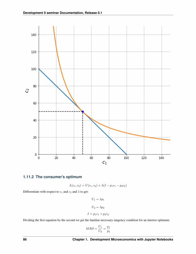
Development II seminar Documentation, Release 0.1
1.11.2 The consumer’s optimum
𝐿(𝑐1, 𝑐2) = 𝑈(𝑐1, 𝑐2) + 𝜆(𝐼 − 𝑝1𝑐1 − 𝑝2𝑐2)
Differentiate with respect to 𝑐1 and 𝑐2 and 𝜆 to get:
𝑈1 = 𝜆𝑝1
𝑈2 = 𝜆𝑝2
𝐼 = 𝑝1𝑐1 + 𝑝2𝑐2
Dividing the first equation by the second we get the familiar necessary tangency condition for an interior optimum:
𝑀𝑅𝑆 =𝑈1
𝑈2=
𝑝1𝑝2
86 Chapter 1. Development Microeconomics with Jupyter Notebooks
Development II seminar Documentation, Release 0.1
Using our earlier expression for the MRS of a Cobb-Douglas indifference curve, substituting this into the budgetconstraint and rearranging then allows us to solve for the Marshallian demand functions:
𝑐1(𝑝1, 𝑝2, 𝐼) =𝛼
𝛼 + 𝛽
𝐼
𝑝1
𝑐1(𝑝1, 𝑝2, 𝐼) =𝛽
𝛼 + 𝛽
𝐼
𝑝2
Interactive plot with sliders (visible if if running on a notebook server):
In [20]: interact(consume_plot,p1=(pmin,pmax,0.1),p2=(pmin,pmax,0.1), I=(Imin,Imax,10),alpha=(0.05,0.95,0.05));
interactive(children=(FloatSlider(value=1.0, description='p1', max=4.0, min=1.0), FloatSlider(value=1.0, descr...
1.11.3 The expenditure function
The indirect utility function:
𝑣(𝑝1, 𝑝2, 𝐼) = 𝑢(𝑐1(𝑝1, 𝑝2, 𝐼), 𝑐2(𝑝1, 𝑝2, 𝐼))
𝑐1(𝑝1, 𝑝2, 𝐼) = 𝛼𝐼
𝑝1
𝑐1(𝑝1, 𝑝2, 𝐼) = (1 − 𝛼)𝐼
𝑝2
𝑣(𝑝1, 𝑝2, 𝐼) = 𝐼 · 𝛼𝛼(1 − 𝛼)1−𝛼 ·[𝑝2𝑝1
]𝛼1
𝑝2
𝐸(𝑝𝑧, 𝑝2, ��) =��
𝛼𝛼(1 − 𝛼)1−𝛼 ·[𝑝2
𝑝1
]𝛼1𝑝2
To minimize expenditure needed to achieve level of utility �� we solve:
min𝑐1,𝑐2
𝑝1𝑐1 + 𝑝2𝑐2
s.t.
𝑢(𝑐1, 𝑐2) = ��
The first order conditions are identical to those we got for the utility maximization problem, and hence we have thesame tangency
𝑈1
𝑈2=
𝛼
1 − 𝛼
𝑐2𝑐1
=𝑝1𝑝2
From this we can solve:
𝑐2 =𝑝1𝑝2
1 − 𝛼
𝛼𝑐1
Now substitute this into the constraint to get:
𝑢
(𝑐1,
𝑝1𝑝2
1 − 𝛼
𝛼𝑐1
)= ��
𝑢
(𝑐1,
𝑝1𝑝2
1 − 𝛼
𝛼𝑐1
)= ��
1.11. Consumer Choice and Intertemporal Choice 87
Development II seminar Documentation, Release 0.1
1.11.4 Intertemporal Consumption choices
We now look at the special case of intertemporal consumption, or consumption of the same good (say corn) overtwo periods. As modeled below the consumer’s income is now given by the market value of and endowment bundle(𝑦1, 𝑦2).
The variables 𝑐1 and 𝑐2 now refer to consumption of (say corn) in period 1 and period 2.
As is typical of intertemporal maximization problems we will use a time-additive utility function. The consumer whohas access to a competitive financial market (they can borrow or save at interest rate 𝑟) maximizes:
𝑈(𝑐1, 𝑐2) = 𝑢(𝑐1) + 𝛿𝑢(𝑐2)
subject to the intertemporal budget constraint:
𝑐1 +𝑐2
1 + 𝑟= 𝑦1 +
𝑦21 + 𝑟
This is just like an ordinary utility maximization problem with prices 𝑝1 = 1 and 𝑝2 = 11+𝑟 . Think of it this way,
the price of corn is $1 per unit in each period, but $1 in period 1 can be placed into savings that will grow to (1 + 𝑟)dollars in period 2. That means that from the standpoint of period 1 owning one unit of corn (or one dollar worth ofcorn) in period 2 is the equivalent of owning 1
1+𝑟 units of corn today (because placed in savings that amount of period1 corn would grow to 1+𝑟
1+𝑟 = 1 units of corn in period 2).
The first order necessary condition for an interior optimum is:
𝑢′(𝑐*1) = 𝛿𝑢′(𝑐*2)
Let’s adopt the widely used Constant-Relative Risk Aversion (CRRA) felicity function of the form:
𝑢 (𝑐𝑡) =
{𝑐1−𝜌
1−𝜌 , if 𝜌 > 0 and 𝜌 = 1
𝑙𝑛 (𝑐) if 𝜌 = 1(1.5)
if 𝜌 = 1
The first order condition then becomes simply
𝑐*1−𝜌 = 𝛿(1 + 𝑟)𝑐*2
−𝜌
or
𝑐*2 = [𝛿(1 + 𝑟)]1𝜌 𝑐*1
From the binding budget constraint we also have
𝑐*2 = 𝐸[𝑦](1 + 𝑟) − 𝑐*1(1 + 𝑟)
where 𝐸[𝑦] = 𝑦1 + 𝑦2
1+𝑟
88 Chapter 1. Development Microeconomics with Jupyter Notebooks
Development II seminar Documentation, Release 0.1
Solving for 𝑐*1 (from the FOC and this binding budget):
𝑐*1 =𝐸[𝑦]
1 + [𝛿(1+𝑟)]1𝜌
1+𝑟
If we simplify to the simple case where 𝛿 = 11+𝑟 , where the consumer discounts future consumption at the same rate as
the market interest rate then at an optimum the consumer will keep their consumption flat at 𝑐*2 = 𝑐*1. If we specializefurther and assume that 𝑟 = 0 then the consumer will set 𝑐*2 = 𝑐*1 = 𝑦1+𝑦2
2
1.11.5 Saving and borrowing visualized
Let us visualize the situation. The consumer has CRRA preferences as described above (summarized by parameters 𝛿and 𝜌 and starts with an income endowment (𝑦1, 𝑦2). The market cost of funds is 𝑟.
A savings case
In the diagram below the consumer is seen to be saving, i.e. 𝑠*1 = 𝑦1 − 𝑐*1 > 0.
In [23]: consume_plot2(r, delta, rho, y1, y2)
1.11. Consumer Choice and Intertemporal Choice 89
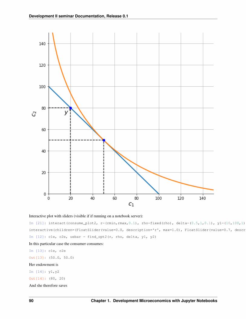
Development II seminar Documentation, Release 0.1
Interactive plot with sliders (visible if if running on a notebook server):
In [21]: interact(consume_plot2, r=(rmin,rmax,0.1), rho=fixed(rho), delta=(0.5,1,0.1), y1=(10,100,1), y2=(10,100,1));
interactive(children=(FloatSlider(value=0.0, description='r', max=1.0), FloatSlider(value=0.7, description='de...
In [12]: c1e, c2e, uebar = find_opt2(r, rho, delta, y1, y2)
In this particular case the consumer consumes:
In [13]: c1e, c2e
Out[13]: (50.0, 50.0)
Her endowment is
In [14]: y1,y2
Out[14]: (80, 20)
And she therefore saves
90 Chapter 1. Development Microeconomics with Jupyter Notebooks
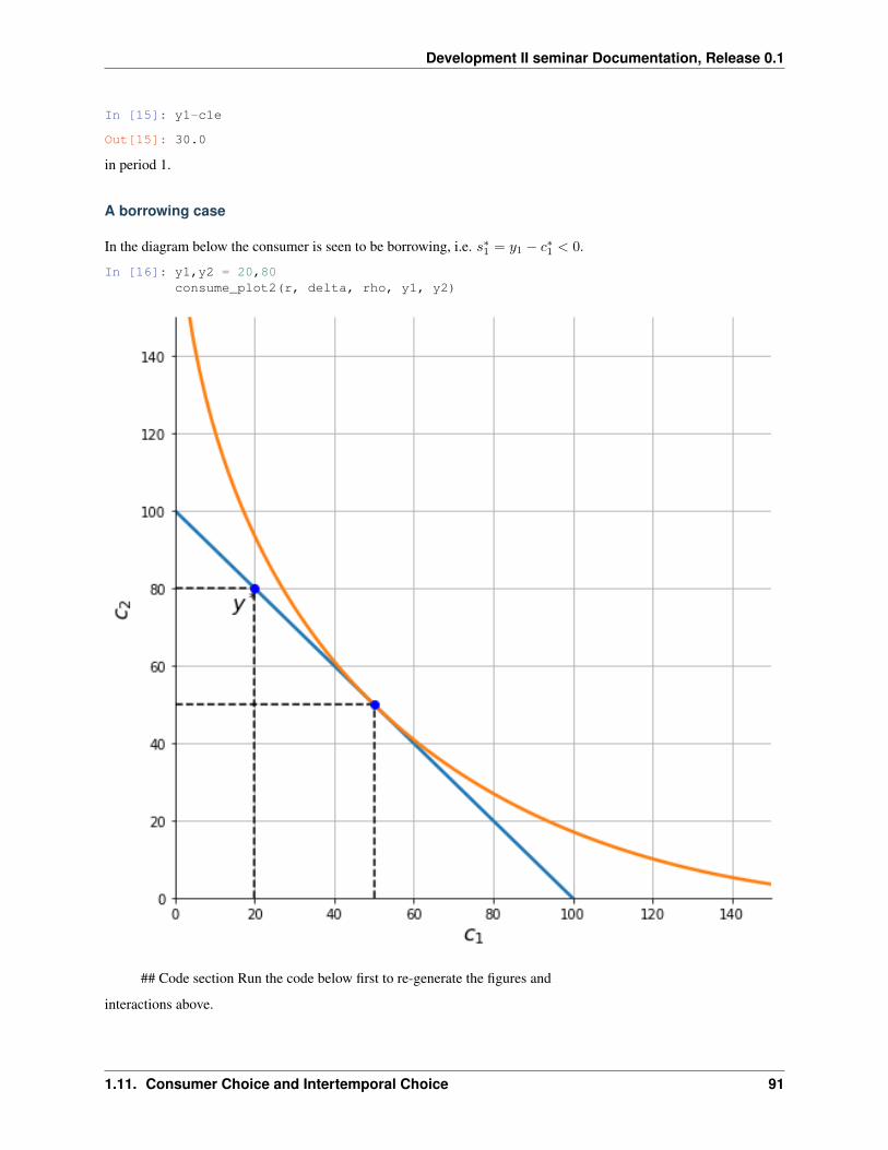
Development II seminar Documentation, Release 0.1
In [15]: y1-c1e
Out[15]: 30.0
in period 1.
A borrowing case
In the diagram below the consumer is seen to be borrowing, i.e. 𝑠*1 = 𝑦1 − 𝑐*1 < 0.
In [16]: y1,y2 = 20,80consume_plot2(r, delta, rho, y1, y2)
## Code section Run the code below first to re-generate the figures and
interactions above.
1.11. Consumer Choice and Intertemporal Choice 91
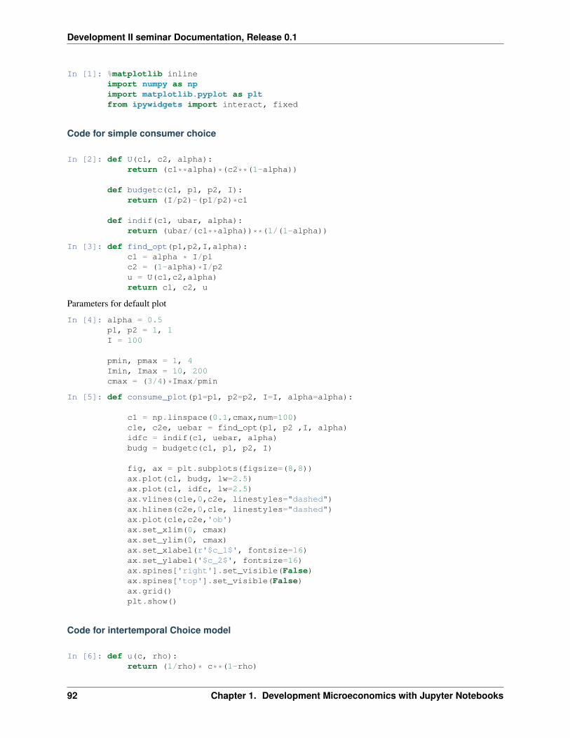
Development II seminar Documentation, Release 0.1
In [1]: %matplotlib inlineimport numpy as npimport matplotlib.pyplot as pltfrom ipywidgets import interact, fixed
Code for simple consumer choice
In [2]: def U(c1, c2, alpha):return (c1**alpha)*(c2**(1-alpha))
def budgetc(c1, p1, p2, I):return (I/p2)-(p1/p2)*c1
def indif(c1, ubar, alpha):return (ubar/(c1**alpha))**(1/(1-alpha))
In [3]: def find_opt(p1,p2,I,alpha):c1 = alpha * I/p1c2 = (1-alpha)*I/p2u = U(c1,c2,alpha)return c1, c2, u
Parameters for default plot
In [4]: alpha = 0.5p1, p2 = 1, 1I = 100
pmin, pmax = 1, 4Imin, Imax = 10, 200cmax = (3/4)*Imax/pmin
In [5]: def consume_plot(p1=p1, p2=p2, I=I, alpha=alpha):
c1 = np.linspace(0.1,cmax,num=100)c1e, c2e, uebar = find_opt(p1, p2 ,I, alpha)idfc = indif(c1, uebar, alpha)budg = budgetc(c1, p1, p2, I)
fig, ax = plt.subplots(figsize=(8,8))ax.plot(c1, budg, lw=2.5)ax.plot(c1, idfc, lw=2.5)ax.vlines(c1e,0,c2e, linestyles="dashed")ax.hlines(c2e,0,c1e, linestyles="dashed")ax.plot(c1e,c2e,'ob')ax.set_xlim(0, cmax)ax.set_ylim(0, cmax)ax.set_xlabel(r'$c_1$', fontsize=16)ax.set_ylabel('$c_2$', fontsize=16)ax.spines['right'].set_visible(False)ax.spines['top'].set_visible(False)ax.grid()plt.show()
Code for intertemporal Choice model
In [6]: def u(c, rho):return (1/rho)* c**(1-rho)
92 Chapter 1. Development Microeconomics with Jupyter Notebooks
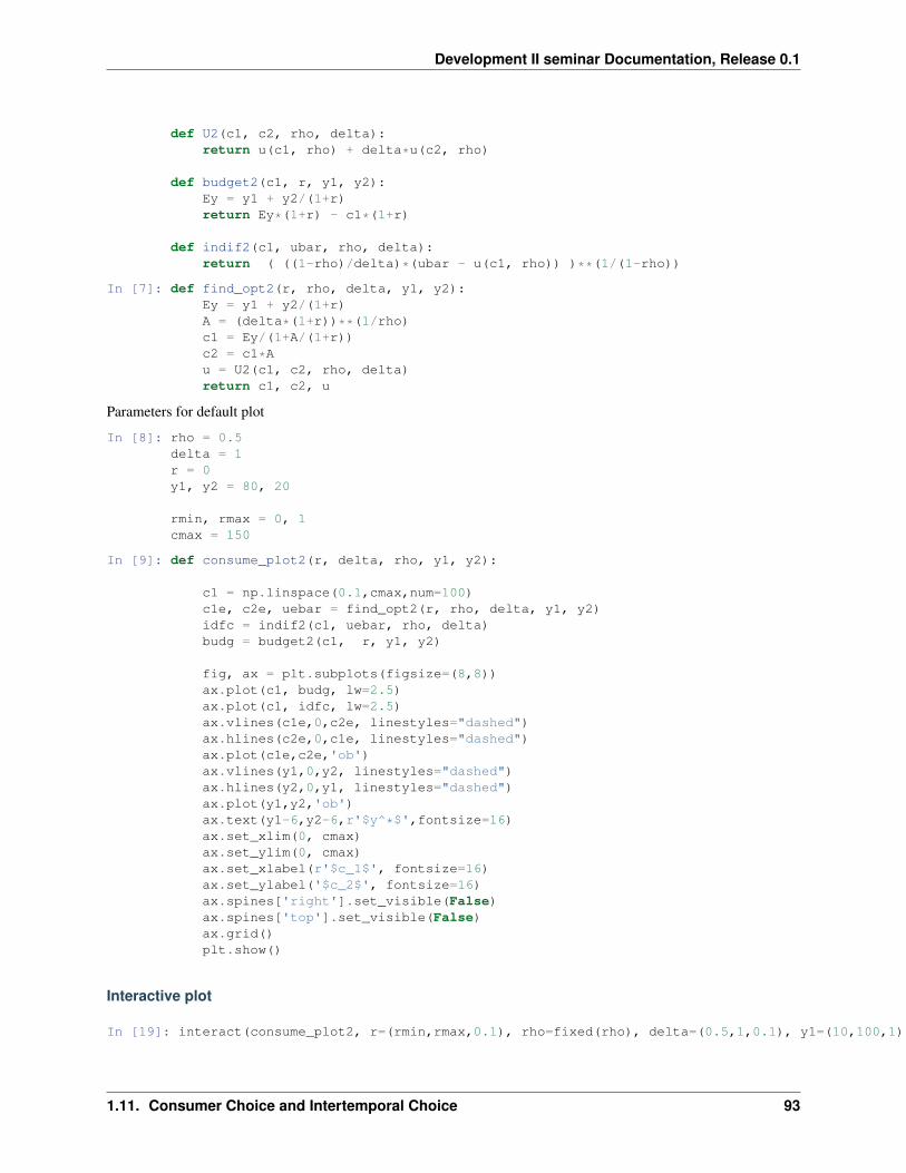
Development II seminar Documentation, Release 0.1
def U2(c1, c2, rho, delta):return u(c1, rho) + delta*u(c2, rho)
def budget2(c1, r, y1, y2):Ey = y1 + y2/(1+r)return Ey*(1+r) - c1*(1+r)
def indif2(c1, ubar, rho, delta):return ( ((1-rho)/delta)*(ubar - u(c1, rho)) )**(1/(1-rho))
In [7]: def find_opt2(r, rho, delta, y1, y2):Ey = y1 + y2/(1+r)A = (delta*(1+r))**(1/rho)c1 = Ey/(1+A/(1+r))c2 = c1*Au = U2(c1, c2, rho, delta)return c1, c2, u
Parameters for default plot
In [8]: rho = 0.5delta = 1r = 0y1, y2 = 80, 20
rmin, rmax = 0, 1cmax = 150
In [9]: def consume_plot2(r, delta, rho, y1, y2):
c1 = np.linspace(0.1,cmax,num=100)c1e, c2e, uebar = find_opt2(r, rho, delta, y1, y2)idfc = indif2(c1, uebar, rho, delta)budg = budget2(c1, r, y1, y2)
fig, ax = plt.subplots(figsize=(8,8))ax.plot(c1, budg, lw=2.5)ax.plot(c1, idfc, lw=2.5)ax.vlines(c1e,0,c2e, linestyles="dashed")ax.hlines(c2e,0,c1e, linestyles="dashed")ax.plot(c1e,c2e,'ob')ax.vlines(y1,0,y2, linestyles="dashed")ax.hlines(y2,0,y1, linestyles="dashed")ax.plot(y1,y2,'ob')ax.text(y1-6,y2-6,r'$y^*$',fontsize=16)ax.set_xlim(0, cmax)ax.set_ylim(0, cmax)ax.set_xlabel(r'$c_1$', fontsize=16)ax.set_ylabel('$c_2$', fontsize=16)ax.spines['right'].set_visible(False)ax.spines['top'].set_visible(False)ax.grid()plt.show()
Interactive plot
In [19]: interact(consume_plot2, r=(rmin,rmax,0.1), rho=fixed(rho), delta=(0.5,1,0.1), y1=(10,100,1), y2=(10,100,1));
1.11. Consumer Choice and Intertemporal Choice 93
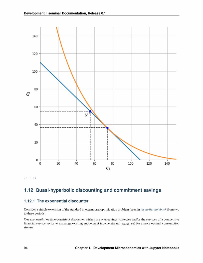
Development II seminar Documentation, Release 0.1
In [ ]:
1.12 Quasi-hyperbolic discounting and commitment savings
1.12.1 The exponential discounter
Consider a simple extension of the standard intertemporal optimization problem (seen in an earlier notebook from twoto three periods.
Our exponential or time-consistent discounter wishes use own-savings strategies and/or the services of a competitivefinancial service sector to exchange existing endowment income stream (𝑦0, 𝑦1, 𝑦2) for a more optimal consumptionstream.
94 Chapter 1. Development Microeconomics with Jupyter Notebooks
Development II seminar Documentation, Release 0.1
The consumer optimization problem is to choose 𝑐0, 𝑐1, 𝑐2 to solve:
max𝑐0,𝑐1,𝑐2
𝑢(𝑐0) + 𝛿𝑢(𝑐1) + 𝛿2𝑢(𝑐2)
𝑠.𝑡.𝑐0 +𝑐1
1 + 𝑟+
𝑐21 + 𝑟
= 𝑦0 +𝑦1
1 + 𝑟+
𝑦21 + 𝑟
where 𝛿 is the consumer’s own personal psychic discount factor and 𝑟 is the financial sector’s opportunity cost of funds.Competitition drives banks to offer earn zero-profits, leading them to offer consumption contract 𝑐* = (𝑐*0, 𝑐
*1, 𝑐
*2) in
exchange for the consumer’s original more volatile income stream 𝑐* = (𝑦0, 𝑦1, 𝑦2) of equal monetary present value.
Let us solve this by setting up a Lagrangean
𝑢(𝑐0) + 𝛿𝑢(𝑐1) + 𝛿2𝑢(𝑐2) − 𝜆
[𝐸𝑦 − 𝑐0 −
𝑐11 + 𝑟
− 𝑐21 + 𝑟
]The first-order necessary conditions for an interior optimum are:
𝑢′(𝑐*0) = 𝜆
𝛿𝑢′(𝑐*1) = 𝜆1
(1 + 𝑟)
𝛿2𝑢′(𝑐*0) = 𝜆1
(1 + 𝑟)2
If it just happens that the consumer’s discount factor 𝛿 has the following relationship to the bank’s opportunity cost offunds 𝑟:
𝛿 =1
1 + 𝑟
Then the first order conditions collapse down to:
u’(c*0) = 𝑢′(𝑐*1) = 𝑢′(𝑐*2) = 𝜆
which of course then implies that the consumer has constant consumption across periods $c_0^* = c_1^* = c_2^* $
It’s easy to establish that if the consumer is sufficiently patient and/or the return to saving is high enough then theconsumer will consume more in later periods:
𝛿 >1
1 + 𝑟then 𝑐*0 < 𝑐*1 < 𝑐*2
and if the situation is reversed so the consumer is relatively impatient and/or the return to savings is low then they willconsume more in earlier periods:
𝛿 >1
1 + 𝑟then 𝑐*0 > 𝑐*1 > 𝑐*2
1.12.2 The CRRA utility case
A Constant-Relative Risk Aversion (CRRA) felicity function is given by:
𝑢 (𝑐𝑡) =
{𝑐1−𝜌
1−𝜌 , if 𝜌 > 0 and 𝜌 = 1
𝑙𝑛 (𝑐) if 𝜌 = 1
if 𝜌 = 1
1.12. Quasi-hyperbolic discounting and commitment savings 95
Development II seminar Documentation, Release 0.1
Te Arrow-Pratt measure of relative risk aversion
𝑅(𝑐) =−𝑐𝑢′′(𝑐)
𝑢′(𝑐)
gives us a measure of how the curvature of the consumers felicity function – or how averse consumers are to risks –changes with wealth (consumption). As its name implies the CRRA function has a constant measure of relative riskaversion given simply by 𝜌.
The elasticity of intertemporal substitution 𝜎 (the responsiveness of the slope of the consumption path to changes inthe interest rate) for a CRRA function is also constant and given simply by:
𝜎 =1
𝜌
If we plug our CRRA felicity function into our earlier derived FOC we can solve to find:
𝑐*1𝑐*0
=𝑐*2𝑐*1
= [𝛿(1 + 𝑟)]1𝜌
Match this to the zero profit condition and we can find a closed form solutions for the consumption path.
1.12.3 Quasi-hyperbolic time-inconsistent preferences
A relatively simple way to model present-biased and time-inconsistent preferences is by moderling prefernces usingquasi-hyperbolic preferences as follows. The key idea in what follows is that the agent’s preferences change fromperiod to period.
The problem can be described in broad terms like this. When first making plans for future consumption choices –say the choice between period period 1 consumption and period 2 consumption – the consumer’s period 0 self wantsto keep consumption smoothly balanced between those two periods. However when period 1 arrives the consumer’spreferences change in a way that makes him/her more impatient or present biased. The new period 1 self consumernow wants to undo the optimal consumption plans laid out by her earlier period 0 self and to choose a new consumptionplan that boosts present (period 1) consumption at the expense of future (period 2) consumption.
The ‘sophisticated’ (quasi) hyperbolic discounter anticipates his own future self’s likely change of heart and this islikely to alter their original period 0 consumption plan. This sets up in effect a conflict or a struggle between theconsumer’s earlier and future selves. The period 0 self acts strategically, anticipating their own later period’s optimalresponses.
The demand for commitment services
Let’s see this formally.The consumer’s “period-0” self wants to choose consumption path (𝑐0, 𝑐1, 𝑐2) to maximize:
𝑢(𝑐0) + 𝛽[𝛿𝑢(𝑐1) + 𝛿2𝑢(𝑐2)]
subject to the earlier described intertemporal budget constraint.
96 Chapter 1. Development Microeconomics with Jupyter Notebooks
Development II seminar Documentation, Release 0.1
This is as before except for the fact that we’ve now introduced a ‘present-bias’ parameter 𝛽 (where 0 < 𝛽 ≤ 1) thattilts the consumer’s preferences toward period zero consumption. Whenever 𝛽 is strictly less than one the consumerwants to smooth preferences in a way that tilts toward period 0 consumption but seeks to keep consumption betweenperiod 1 and 2 more balanced.
When period 1 rolls around however the consumer’s preferences over remaining consumption bundles change. Theperiod 1 self now wants to re-arrange remaining consumption to now maximize:
𝑢(𝑐1) + 𝛽𝛿𝑢(𝑐2)
While the period-0 self wanted to trade off period 1 and period 2 consumption to equalize marginal utilities like this:
𝑢′(𝑐*1) = 𝛿(1 + 𝑟)𝑢′(𝑐*2)
the new period-1 self now pefers to tradeoff like this:
𝑢′(𝑐*1) = 𝛽𝛿(1 + 𝑟)𝑢′(𝑐*2)
The 𝛽 on the right-hand side of the last equation means the period 1 consumer now values period 2 consumption lessrelative to period 1 consumption compared to his period 0 self. Compared to the period-0 self’s plans the new period-1consumer wants to ‘raid-savings’ and/or ‘take out a new loan’.
Lets look again at the CRRA case under the special assumption that 𝛿 = 11+𝑟 and 𝑟 = 0 (and hence 𝛿 = 1. These
last assumptions are without loss of generality and done only to simplify the math and spotlight the key mechanismsat work.
Let’s assume also that the period zero consumer can contract with a bank and that the bank can credibly commit to notrenegotiating the terms of the contract even when the consumer’s period 1 self comes begging for the bank to do so.
In this case the problem is exactly as described in the earlier section. The period 0 consumer maximizes
𝑢(𝑐0) + 𝛽[𝛿𝑢(𝑐1) + 𝛿2𝑢(𝑐2)]
subject to the intertemporal budget constraint.
When 𝛿 = 11+𝑟 the period 0 consumer would like to keep consumption between period 1 and period 2 flat. The first
order conditions now reduce to:
𝑐*1 = 𝛽1𝜌 𝑐*0
𝑐*2 = 𝑐*1
Substituting these into the binding budget constraint yields:
𝑐*0 =𝐸[𝑦]
1 + 𝛽1𝜌
𝑐*1 = 𝑐*2 = 𝛽1𝜌 𝑐*0
We call this the full commitment contract.
The financial intermediary who offers such a contract is really providing two services to consumer’s period 0 self:they’re helping the consumer to smooth consumption between period zero and later periods and they’re also helpingthe consumer resist his period 1 self’s temptation to disrupt this optimal consumption plan.
For example suppose that consumer endowment income is such that she finds it optimum to save in period 0 and thenfinance constant consumption out of endowment income and savings in period 1 and 2. When period 1 rolls aroundthe consumer’s period 1 self present bias would tempt them to want to ‘raid savings’ and/or take out a new loan toboost period 1 consumption at the expense of period 2 consumption.
1.12. Quasi-hyperbolic discounting and commitment savings 97
Development II seminar Documentation, Release 0.1
To see this formally note that under the full commitment contract the consumer enters the period with contractualclaims to the remaining consumption stream (𝑐*1, 𝑐
*2) = (𝑐*, 𝑐*). If they could however the period 1 self would re-
contract with this bank (or another) to choose another contract (𝑐1, 𝑐2) that solves:
max𝑐1,𝑐2
𝑢(𝑐1) + 𝛽𝑢(𝑐2)
subject to
𝑐1 +𝑐2
1 + 𝑟≤ 𝑐* +
𝑐*
1 + 𝑟
The first order conditions for this problem are
𝑢′(𝑐1) = 𝛽𝑢′(𝑐2)
which in the CRRA case requires 𝑐2 = 𝛽1𝜌 𝑐1
which is clearly not satisfied along the original contract which had (𝑐*1, 𝑐*2) = (𝑐*, 𝑐*)
Substituting the FOC into the new period 1 budget constraint we can arrive at a solution or reaction function that statesthat when the period 1 self enters the period with claims 𝑐1, 𝑐2 they will want to renegotiate to:
𝑐1 =𝑐1 + 𝑐2
1 + 𝛽1𝜌
𝑐2 = 𝛽1𝜌 𝑐1
If this renegotiation takes place then the period 1’s welfare would increase but at the expense of period 0’s welfare,since period 0’s optimal consumption plan would have been undone.
From this discussion it should be clear that the period 0 self would like to have banks compete for her business inperiod 0 but offer a full-commitment contract which in practice means being locked into an exclusive relationship (ifthe relationship were not exclusive then the period 1 self would approach a second bank in period 1 and ask them to‘buy out’ and then renegotiate their contract with the first bank.
1.12.4 More detailed analysis
Much more detail on the analysis of contracts like this can be found in our 2016 working paper (with Karna Basu)entitled “Sticking to the Contract: Nonprofit vs For-profit Banks and Hyperbolic Discounters.” A github repository isavailable with code and jupyter notebooks describing some of that analysis. I draw on that here, but most of the detailsof the methods are in those other notebooks.
1.12.5 Commitment Savings products
Many economists believe that time-inconsistent preferences drive people to have to struggle with important issues ofself-control that affects their ability to reach savings goals, and generates a demand for commitment services. Indeedsome economiss have gone so far as to argue that these problems are ubiquitous and that one reason for the demandfor microfinance services is that they provide individuals with the discipline and commitment mechanisms that canhelp them with these problems of self-control.
Rotating Savings and Credit Associations (ROSCAs) for example place individuals into savings groups and then createpressures and social sanctions to help individuals achieve savings goals. Iterant savings collectors may serve a similarpurpose. Some have even suggested that many microcredit loans which advance loans to individuals and then putthem on tight weekly repayment schedules may be popular not so much because they are releasing the individual froma binding credit constraint as because they are helping the individual ‘borrow to save.’ In this type of scenario theindividual wants to save up to buy say a refrigerator or other household appliance but cannot find the discipline to save
98 Chapter 1. Development Microeconomics with Jupyter Notebooks
Development II seminar Documentation, Release 0.1
up for the item themselves. A microcredit loan allows them to buy the refrigerator outright and then places them on astrict repayment schedule that commits the individual to putting aside the fraction of weekly income toward the itemthat they might have otherwise struggled to do on their own.
In all these stories the availabiliy of commitment contracts provides additional value to the consumer, value that theymay be willing to pay for.
In the following section I will illustrate some of these ideas with contracts that we will solve for and illustrate for theCRRA case. The code for much of what follows is in the Contract.py module described in greater detail in the githubrepo.
In [5]: import Contract
Lets look at a competive contracting situation where 𝛽 = 0.8 and 𝜌 = 0.5
In [9]: cC = Contract.Competitive(beta = 0.8)cC.rho = 0.5
Now lets give the individual an endowment income of (𝑦0, 𝑦1, 𝑦2) = (150, 100, 50)
In [15]: cC.y = [150,100,50]
The full commitment contract is:
In [21]: cCF = cC.fcommit(); cCF
Out[21]: array([ 131.57894737, 84.21052632, 84.21052632])
Note how this involves some saving in period 0 (𝑦0 = 150 and consumption 𝑐0 = 131.6) as well as additional savingfor period 2.
If for some reason period 0 self agreed to this contract (sincerely believing that it would never be renegotiated) butthen suddenly to everyone’s surprise period 1 self had an opportunity to renegotiate the continuation of this contract,they would renegotiate to the following contract:
In [22]: cCR = cC.reneg(cCF); cCR
Out[22]: array([ 131.57894737, 101.44337644, 64.92376092])
We can see here how period 1 self ‘raids’ the savings that the period 0 self had intended should be passed onto period 2consumption. The period 1 self boosts period 1 consumption from 84 to 101. Rather than pass 34 units of consumptioninto period 2 only 20 units are now passed.
If the bank cannot credibly commit to not renegotiate the contract then the sophisticated time-inconsistent consumerwill defensively alter their consumption plans to try to thwart their future self’s strategic renegotiations. The period0 consumer will insist on renegotiation proof contracts which will impose an additional constraint on the problem,namely that no bank find it profitable to renegotiate the contract. In general this will be achieved by in a sense‘surrendering’ to their future self’s bias tilt toward period 1 consumption.
Details in the paper and in class lecture on the shape of this constraint.
The important thing to understand is that adding any constraint to the problem can only lower consumer welfare andpush us away from the full-commitment optimum.
For the present setup the renegotiation proof contract can be solved for to find:
In [31]: cCRP = cC.reneg_proof().x; cCRP
Out[31]: array([ 122.59354576, 108.17462856, 69.23182568])
Compare to the full commitment contract this contract involves more savings pased from from period 0 to period 1 butmuch less savings passed from period 1 to period 2. Total savings (period 0 plus period 1 savings) are higher whencredible commitment savings devices are available compared to when not.
1.12. Quasi-hyperbolic discounting and commitment savings 99
Development II seminar Documentation, Release 0.1
1.12.6 Replicating Ashraf, Karlan and Yin (2006) Commitment Savings paper
Ashraf, Karlan and Yin (2006) “Tying Odysseus to the Mast: Evidence from a Commitment Savings Product in thePhilippines,” *Quarterly Journal of Economics.
What follows are incomplete notes. . . just some pieces of the puzzle needed to replicate the paper. I hope to improveon this in time and I just offer this here so that you might form an idea on how this might be done. Note that I amusing the ipystata library which requires Stata to be running in the background. This seems to only be possible to doon Windows machines as described in the ipystata library.
The Stata dataset and code replication files have been made available by the authors via the Harvard Dataverse here
Notes to self: Files in D:
Drive
_S15
renamed
“D:
Drive
_S15
_011204_1.dta” “D:
Drive
_S15
_011204_080404_1.dta” “D:
Drive
_S15
_080404_1.dta”
The posted files are Stata version 14. These can be opened by python pandas but not by older versions of Stata.
In [2]: %matplotlib inlineimport seaborn as snsimport pandas as pdimport ipystataimport statsmodels.formula.api as sm
Open the datasets
One disadvantage of proprietary software is that you often cannot open a dataset saved with a later version of thesoftware unless you pay to upgrade the software. I’m going to load the Stata dataset into a python pandas dataframeusing its read_stata method and then pass the dataset into the running Stata session (which on my home machine isStata 11).
In [7]: #df = pd.read_stata(r"G:\GC\Dev-II\notebooks\seedanalysis_011204_1_v12.dta")df = pd.read_stata(r"G:\GC\Dev-II\notebooks\data\savings1.dta")
In [8]: regVI_1 = 'balchange ~ treatment + marketing'model = sm.ols(regVI_1, df)fitted = model.fit(cov_type='HC1')print(fitted.summary())
100 Chapter 1. Development Microeconomics with Jupyter Notebooks
Development II seminar Documentation, Release 0.1
OLS Regression Results==============================================================================Dep. Variable: balchange R-squared: 0.002Model: OLS Adj. R-squared: 0.001Method: Least Squares F-statistic: 2.901Date: Tue, 29 Mar 2016 Prob (F-statistic): 0.0553Time: 17:00:31 Log-Likelihood: -16270.No. Observations: 1777 AIC: 3.255e+04Df Residuals: 1774 BIC: 3.256e+04Df Model: 2Covariance Type: HC1==============================================================================
coef std err z P>|z| [95.0% Conf. Int.]------------------------------------------------------------------------------Intercept 40.6257 61.676 0.659 0.510 -80.257 161.509treatment 234.6785 101.748 2.306 0.021 35.256 434.101marketing 184.8506 146.982 1.258 0.209 -103.228 472.929==============================================================================Omnibus: 3458.895 Durbin-Watson: 0.051Prob(Omnibus): 0.000 Jarque-Bera (JB): 5716807.283Skew: 14.932 Prob(JB): 0.00Kurtosis: 279.259 Cond. No. 4.24==============================================================================
Warnings:[1] Standard Errors are heteroscedasticity robust (HC1)
In [33]: model = sm.ols('balchange ~ treatment', df[(df.treatment ==1) | (df.marketing ==1)])fitted = model.fit(cov_type='HC1')print(fitted.summary())
OLS Regression Results==============================================================================Dep. Variable: balchange R-squared: 0.000Model: OLS Adj. R-squared: -0.001Method: Least Squares F-statistic: 0.1020Date: Thu, 24 Mar 2016 Prob (F-statistic): 0.750Time: 23:43:38 Log-Likelihood: -12115.No. Observations: 1308 AIC: 2.423e+04Df Residuals: 1306 BIC: 2.424e+04Df Model: 1Covariance Type: HC1==============================================================================
coef std err z P>|z| [95.0% Conf. Int.]------------------------------------------------------------------------------Intercept 225.4763 133.405 1.690 0.091 -35.992 486.944treatment 49.8279 156.027 0.319 0.749 -255.979 355.635==============================================================================Omnibus: 2498.290 Durbin-Watson: 0.056Prob(Omnibus): 0.000 Jarque-Bera (JB): 3202671.430Skew: 14.153 Prob(JB): 0.00Kurtosis: 243.756 Cond. No. 3.11==============================================================================
Warnings:[1] Standard Errors are heteroscedasticity robust (HC1)
Table 6: Impact: 6 months
1.12. Quasi-hyperbolic discounting and commitment savings 101
Development II seminar Documentation, Release 0.1
1.13 Notes on Incentive Contracts and Corruption
Many public policy issues in developing countries be understood and modeled as asymmetric information problemswhere Principal - Monitor - Agent contract structures must be employed.
Consider for example a central government that launches a project either to improve rural roads (as in Olken, 2007) orperhaps instead a project to carry out a campaign to distribute anti-malaria mosquito nets.
For either type of project the government will make funds available to local communities across the country but mustrely on local agents (e.g. local contractors or officials) to implement the projects. The government may have a verygood idea of how much it costs to repair a kilometer or make and distribute 1000 mosquito nets but typically cannotmonitor whether the local agents ‘diligently’ carry out the project to specification or not. The government will in theend see if the project has succeeded or failed, and the project is much more likely to succeed if the local contractorhas carried out the contract to specification, but the government cannot directly verify whether this has been the caseor not. This moral hazard situation means that the government can only put local agents on outcome-contingent andnot action-contingent contracts.
For example after the local road repair project is completed the government will be able to see if the project succeeded(e.g. the bridge was not washed away this year when the river floods) or whether it failed (it did not wash away). Butthe government can not directly observe the agent’s level of diligence in the project – for example whether they builtthe bridge to specification with the allocated funds or if they perhaps substituted shoddier building materials to divertfunds to private gain) because the project’s outcome is probabilistic.
Similarly in an anti-malarial campaign the local agent might claim to have made and distributed 1000 mosquito netsbut in fact it only made and distributed 500. All the government can do is observe whether the number of malariacases has been reduced (success) or increased or stayed the same compared to earlier years.
Let’s model this principal-agent problem using the same simple model we used to describe tenancy and credit contracts.
The government advances 𝐼 in funds to an agent to purchase materials to carry out the project. If the agent diligentlycarries out the project to specification the project succeeds with probability 𝑝 in which case the community receivesbenefit 𝑋𝑠 or it fails with probability 1 − 𝑝 in which case the community receives benefits of only 𝑋𝑓 < 𝑋𝑠.
If the agent is not diligent they divert project funds and/or put in less effort all of which allows them to capture privatebenefits 𝐵. Furthermore when the agent is non-diligent the project succeeds with only probability 𝑞 (in which case thecommunity again receives benefit 𝑋𝑠) or it fails with probability 1− 𝑞 (in which case the community receives benefitsof only 𝑋𝑓 < 𝑋𝑠).
Since the government can only observe project outcomes and not the choice of diligence the principal can only get theagent to be diligent by offering a contract that rewards the agent sufficiently more for project successes as for failures,in order to want to make the agent want to on their own raise the probability of success via their choice of diligence.
The government aims to maximize the expected value of community benefits minus the cost of the investment fundsand the cost of renumerating the agent:
max𝑐𝑠,𝑐𝑓
𝑝(𝑋𝑠 − 𝑐𝑠) + (1 − 𝑝)(𝑋𝑓 − 𝑐𝑓 ) − 𝐼
subject to the agent’s participation (PC) constraint:
𝑝𝑐𝑠 + (1 − 𝑝)𝑐𝑓 ≥ ��
Without loss of generality in what follows we will set �� = 0, so in the ideal of circumstances the government wouldbe able to hire the agent away from their next best opportunity by paying them amount normalized to zero.
and an incentive compatibility (IC) constraint:
𝑝𝑐𝑠 + (1 − 𝑝)𝑐𝑓 ≥ 𝑞𝑐𝑠 + (1 − 𝑞)𝑐𝑓 + ��
102 Chapter 1. Development Microeconomics with Jupyter Notebooks

Development II seminar Documentation, Release 0.1
Note that we will at times write this problem compactly as:
max𝑐𝑠,𝑐𝑓
𝐸(𝑋|𝑝) − 𝐸(𝑐|𝑝) − 𝐼
s.t.
𝐸(𝑐|𝑝) ≥ ��
𝐸(𝑐|𝑝) ≥ 𝐸(𝑐|𝑞) + ��
The IC constraint can be rewritten:
𝑐𝑠 ≥ 𝑐𝑓 +��
𝑝− 𝑞
This can be satisfied at minimum cost when this constraint binds. This tells us that in the event of project successthe agent must receive a ‘bonus’ of ��
𝑝−𝑞 over what they get paid for failure outcomes. This higher reward for successcompared to failure is what induces the agent to want to be diligent and increase the probability of success from 𝑞 to𝑝. The contractual cost of this renumeration strategy is then 𝑝𝑐𝑠 + (1 − 𝑝)𝑐𝑓 or:
𝐸(𝑐|𝑝) = 𝑐𝑓 + 𝑝��
∆
where ∆ = 𝑝− 𝑞which then means that the expected net benefit of the government project is:
𝐸(𝑋|𝑝) − 𝐼 − 𝑐𝑓 − 𝑝��
∆
Note that we earlier normalized the agent’s next best employment opportunity to a renumeration of zero. If thegovernment could get local agents to competitively bid against each other for the government contract the agent’scontract could be made to bind, but this in turn would require:
𝑐𝑓 = −𝑝��
∆+ ��
𝑐𝑠 = (1 − 𝑝)��
∆+ ��
One way to think of this is that the agent is made to pay a fine of −𝑝 ��Δ when the project fails while if the project
succeeds she earns a reward of (1 − 𝑝) ��Δ
A possible problem with this type of project is that it may be difficult for the government to impose a penalty on agentswhen the project fails (e.g. the local contractor leaves town when the bridge collapses or the incidence of malaria casessurges). One way to try to resolve that problem is by asking local contractors to post a bond but this solution may behard to implement particularly in poor communities where the agents are poor to start with.
The consequence of not being able to impose a fine when the project fails is that we have to now impose yet anotherconstraint on the contract design problem, a limited liability constraint of the form
𝑐𝑓 ≥ 0
for example if the heaviest fine that can be imposed is to pay the local agent nothing when the project fails. Thelowest cost way to renumerate the agent will be for this limited liability constraint and the incentive compatibilityconstraints to bind (to set the punishment as high as possible and the bonus as low as possible, compatible withmaintaining incentives. With 𝑐𝑓 = 0 an extra bonus must now be paid folowing success outcomes to contine to satisfythe incentive constraint. But this increases the expected cost of renumeration and reduces expected benefits from theproject to:
𝐸(𝑋|𝑝) − 𝐼 − 𝑝��
∆
The last term 𝑝 ��Δ is sometimes referred to as an ‘information rent’ that must be paid to the agent that arises due to the
asymmetric information problem.
1.13. Notes on Incentive Contracts and Corruption 103
Development II seminar Documentation, Release 0.1
1.13.1 An Example
In [1]: %matplotlib inlineimport matplotlib.pyplot as pltimport numpy as npfrom ipywidgets import interact, fixed
In [97]: def E(xs,xf,p):"""Expectation operator """return p*xs + (1-p)*xf
Consider a project with the following characteristics:
In [100]: I = 75 # Lump sum investment to start projectXs = 100 # project success returnXf = 0 # project failure returnp = 0.95 # probability of success when diligentq = 0.50 # probability of success when non-diligentEX = E(Xs,Xf,p) # Gross expected project returnubar = 5 # Consumer reservation incomeB = 10 # private benefits to being non-diligent
In [84]: print('Expected returns Diligent (p): {}, Non-diligent (q): {}'.format(E(Xs,Xf,p), E(Xs,Xf,q)))
Expected returns Diligent (p): 95.0, Non-diligent (q): 50.0
This project fails only 1 percent of the time when the agent is non-diligent (corrupt) but fails 50 percent of the timewhen they are non-diligent (corrupt). We associate non-diligence with an opportunity to divert �� in funds to privateuses.
In [85]: B = 10
As derived above the optimal renumeration contract calls for the agent to pay a big fine for failure and earn a positivereward for success:
In [111]: cf = -p*B/(p-q) + ubarcs = (1-p)*B/(p-q) + ubar
In [112]: print('(c_f, c_s) =({:5.1f}{:5.1f})'.format(cf, cs))
(c_f, c_s) =(-16.1 6.1)
In [113]: print('consumer and bank expected payments:')E(cs,cf,p), E(Xs-cs, Xf-cf,p) - I
consumer and bank expected payments:
Out[113]: (5.0, 15.0)
In expectation this covers the agent’s opportunity cost of funds ��. Since the incentive compatibility constraint is met(by construction) when she is diligent:
Diagram
In [89]: def zeroprofit(c):return EX/p -((1-p)/p)*c - I/p
def IC(c):return c + B/(p-q)
def BPC(c,ubar):return ubar/p - ((1-p)/p)*c
104 Chapter 1. Development Microeconomics with Jupyter Notebooks
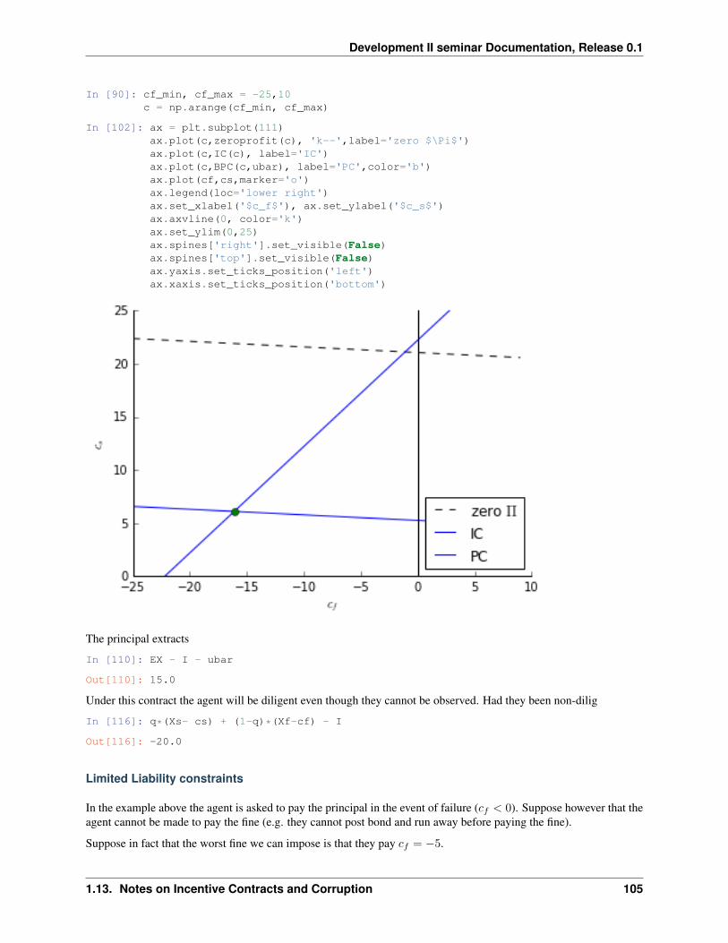
Development II seminar Documentation, Release 0.1
In [90]: cf_min, cf_max = -25,10c = np.arange(cf_min, cf_max)
In [102]: ax = plt.subplot(111)ax.plot(c,zeroprofit(c), 'k--',label='zero $\Pi$')ax.plot(c,IC(c), label='IC')ax.plot(c,BPC(c,ubar), label='PC',color='b')ax.plot(cf,cs,marker='o')ax.legend(loc='lower right')ax.set_xlabel('$c_f$'), ax.set_ylabel('$c_s$')ax.axvline(0, color='k')ax.set_ylim(0,25)ax.spines['right'].set_visible(False)ax.spines['top'].set_visible(False)ax.yaxis.set_ticks_position('left')ax.xaxis.set_ticks_position('bottom')
The principal extracts
In [110]: EX - I - ubar
Out[110]: 15.0
Under this contract the agent will be diligent even though they cannot be observed. Had they been non-dilig
In [116]: q*(Xs- cs) + (1-q)*(Xf-cf) - I
Out[116]: -20.0
Limited Liability constraints
In the example above the agent is asked to pay the principal in the event of failure (𝑐𝑓 < 0). Suppose however that theagent cannot be made to pay the fine (e.g. they cannot post bond and run away before paying the fine).
Suppose in fact that the worst fine we can impose is that they pay 𝑐𝑓 = −5.
1.13. Notes on Incentive Contracts and Corruption 105
Development II seminar Documentation, Release 0.1
When that is the case the cheapest way to satisfy the incentive compatibility constraint is to set:
In [117]: cf = -5cs = -5 + B/(p-q)
Which then means that in expectation the agent earns an information rent of
In [118]: E(cs,cf,p)
Out[118]: 16.111111111111114
This is above their reservation utility 𝑏𝑎𝑟𝑢 and this contract is therefore quite a bit more expensive to the principal.Their net return is now
𝐸(𝑋, 𝑝) − 𝐼 − 𝐸(𝐶, 𝑝)
𝐸(𝑋, 𝑝) − 𝐼 − 𝑝/(𝑝− 𝑞)
And the net benefits to the project are greatly reduced to:
In [119]: EX - I - E(cs,cf,p)
Out[119]: 3.8888888888888857
The net benefits have been reduced by the heavy cost of incentive contract to keep the agent diligent or non-corrupt.
But this is still better than allowing the agent to be corrupt.
In [121]: q*(Xs-cs)+(1-q)*(Xf-cf) - I
Out[121]: -31.111111111111114
As we can see from the diagram above the principal can contract with agents who face limited liability but they earnless from agents where the LL constraint binds. The limited liability constraint means the agent must earn a rent inexcess of their reservation utility.
Suppose the most we can take away from the agent is an amount 𝐴, equal for example to the amount of resources thatcan be seized or that they posted as bond or collateral.
The cheapest way to satisfy the IC is then:
𝑐𝑓 = −𝐴
𝑐𝑠 = −𝐴 + 𝐵/(𝑝− 𝑞)
Which implies the agent’s expected repayment is:
𝐸(𝑐|𝑝) = −𝐴 +𝑝𝐵
𝑝− 𝑞
which will be more than their reservation wage �� as long as 𝐴 < 𝑝 𝐵𝑝−𝑞 ��
Minimum collateral requirement
What is the minimum collateral requirement below which the contract cannot both satisfy the incentive compatibilityconstraint and guarantee at least zero profits to the principal?
Substitute the expected repayment under limited liability (above) into the principal’s zero profit condition and solve forA (on the diagram above this is the 𝑐𝑓 at the intersection of the IC constraint and the principal’s zero profit condition:
𝐸(𝑋|𝑝) − 𝐸(𝑐|𝑝) − 𝐼 = 0
𝐸(𝑋|𝑝) + 𝐴− 𝑝��𝑝−𝑞 − 𝐼 = 0
𝐴 =𝑝𝐵
𝑝− 𝑞− [𝐸(𝑋|𝑝) − 𝐼]
106 Chapter 1. Development Microeconomics with Jupyter Notebooks
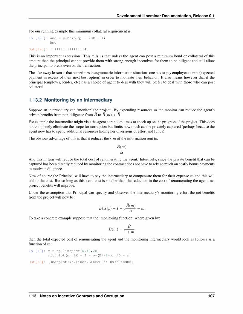
Development II seminar Documentation, Release 0.1
For our running example this minimum collateral requirement is:
In [123]: Amc = p*B/(p-q) - (EX - I)Amc
Out[123]: 1.1111111111111143
This is an important expression. This tells us that unless the agent can post a minimum bond or collateral of thisamount then the principal cannot provide them with strong enough incentives for them to be diligent and still allowthe principal to break even on the transaction.
The take away lesson is that sometimes in asymmetric information situations one has to pay employees a rent (expectedpayment in excess of their next best option) in order to motivate their behavior. It also means however that if theprincipal (employer, lender, etc) has a choice of agent to deal with they will prefer to deal with those who can postcollateral.
1.13.2 Monitoring by an intermediary
Suppose an intermediary can ‘monitor’ the project. By expending resources 𝑚 the monitor can reduce the agent’sprivate benefits from non-diligence from �� to ��(𝑚) < ��.
For example the intermediar might visit the agent at random times to check up on the progress of the project. This doesnot completely eliminate the scope for corruption but limits how much can be privately captured (perhaps because theagent now has to spend additional resources hiding her diversions of effort and funds).
The obvious advantage of this is that it reduces the size of the information rent to:
��(𝑚)
∆
And this in turn will reduce the total cost of renumerating the agent. Intuitively, since the private benefit that can becaptured has been directly reduced by monitoring the contract does not have to rely so much on costly bonus paymentsto motivate diligence.
Now of course the Principal will have to pay the intermediary to compensate them for their expense 𝑚 and this willadd to the cost. But so long as this extra cost is smaller than the reduction in the cost of renumerating the agent, netproject benefits will improve.
Under the assumption that Principal can specify and observer the intermediary’s monitoring effort the net benefitsfrom the project will now be:
𝐸(𝑋|𝑝) − 𝐼 − 𝑝��(𝑚)
∆−𝑚
To take a concrete example suppose that the ‘monitoring function’ where given by:
��(𝑚) =��
1 + 𝑚
then the total expected cost of renumerating the agent and the monitoring intermediary would look as follows as afunction of 𝑚:
In [12]: m = np.linspace(0,10,20)plt.plot(m, EX - I - p*(B/(1+m))/D - m)
Out[12]: [<matplotlib.lines.Line2D at 0x759e8d0>]
1.13. Notes on Incentive Contracts and Corruption 107
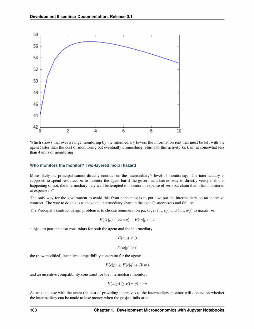
Development II seminar Documentation, Release 0.1
Which shows that over a range monitoring by the intermediary lowers the information rent that must be left with theagent faster than the cost of monitoring but eventually diminishing returns to this activity kick in (at somewhat lessthan 4 units of monitoring).
Who monitors the monitor? Two-layered moral hazard
More likely the principal cannot directly contract on the intermediary’s level of monitoring. The intermediary issupposed to spend resources 𝑚 to monitor the agent but if the government has no way to directly verify if this ishappening or not, the intermediary may well be tempted to monitor at expense of zero but claim that it has monitoredat expense 𝑚?
The only way for the government to avoid this from happening is to put also put the intermediary on an incentivecontract. The way to do this is to make the intermediary share in the agent’s successess and failures.
The Principal’s contract design problem is to choose renumeration packages (𝑐𝑠, 𝑐𝑓 ) and (𝑤𝑠, 𝑤𝑓 ) to maximize:
𝐸(𝑋|𝑝) − 𝐸(𝑐|𝑝) − 𝐸(𝑚|𝑝) − 𝐼
subject to participation constraints for both the agent and the intermediary
𝐸(𝑐|𝑝) ≥ 0
𝐸(𝑤|𝑝) ≥ 0
the (now modified) incentive compatibility constraint for the agent:
𝐸(𝑐|𝑝) ≥ 𝐸(𝑐|𝑞) + ��(𝑚)
and an incentive compatibility constraint for the intermediary monitor:
𝐸(𝑤|𝑝) ≥ 𝐸(𝑤|𝑞) + 𝑚
As was the case with the agent the cost of providing incentives to the intermediary monitor will depend on whetherthe intermediary can be made to lose money when the project fails or not.
108 Chapter 1. Development Microeconomics with Jupyter Notebooks
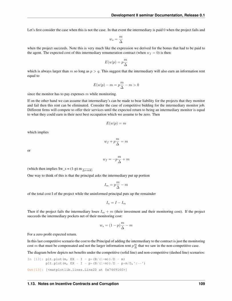
Development II seminar Documentation, Release 0.1
Let’s first consider the case when this is not the case. In that event the intermediary is paid 0 when the project fails and
𝑤𝑠 =𝑚
∆
when the project succeeds. Note this is very much like the expression we derived for the bonus that had to be paid tothe agent. The expected cost of this intermediary renumeration contract (when 𝑤𝑓 = 0) is then:
𝐸(𝑤|𝑝) = 𝑝𝑚
∆
which is always larger than 𝑚 so long as 𝑝 > 𝑞. This suggest that the intermediary will also earn an information rentequal to
𝐸(𝑤|𝑝) −𝑚 = 𝑝𝑚
∆−𝑚 > 0
since the monitor has to pay expenses 𝑚 while monitoring.
If on the other hand we can assume that intermediary’s can be made to bear liability for the projects that they monitorand fail then this rent can be eliminated. Consider the case of competitive bidding for the intermediary monitor job.Different firms will compete to offer their services until the expected return to being an intermediary monitor is equalto what they could earn in their next best occupation which we assume to be zero. Then
𝐸(𝑤|𝑝) = 𝑚
which implies
𝑤𝑓 + 𝑝𝑚
∆= 𝑚
or
𝑤𝑓 = −𝑝𝑚
∆+ 𝑚
(which then implies $w_s = (1-p) mΔ+𝑚$)
One way to think of this is that the principal asks the intermediary put up portion
𝐼𝑚 = 𝑝𝑚
∆−𝑚
of the total cost I of the project while the uninformed principal puts up the remainder
𝐼𝑢 = 𝐼 − 𝐼𝑚
Then if the project fails the intermediary loses 𝐼𝑚 + 𝑚 (their investment and their monitoring cost). If the projectsucceeds the intermediary pockets net of their monitoring cost:
𝑤𝑠 = (1 − 𝑝)𝑚
∆−𝑚
For a zero profit expected return.
In this last competitive scenario the cost to the Principal of adding the intermediary to the contract is just the monitoringcost 𝑚 that must be compensated and not the larger information rent 𝑝𝑚
Δ that we saw in the non-competitive case.
The diagram below depicts net benefits under the competitive (solid line) and non-competitive (dashed line) scenarios:
In [13]: plt.plot(m, EX - I - p*(B/(1+m))/D - m)plt.plot(m, EX - I - p*(B/(1+m))/D - p*m/D,'r--')
Out[13]: [<matplotlib.lines.Line2D at 0x7469160>]
1.13. Notes on Incentive Contracts and Corruption 109
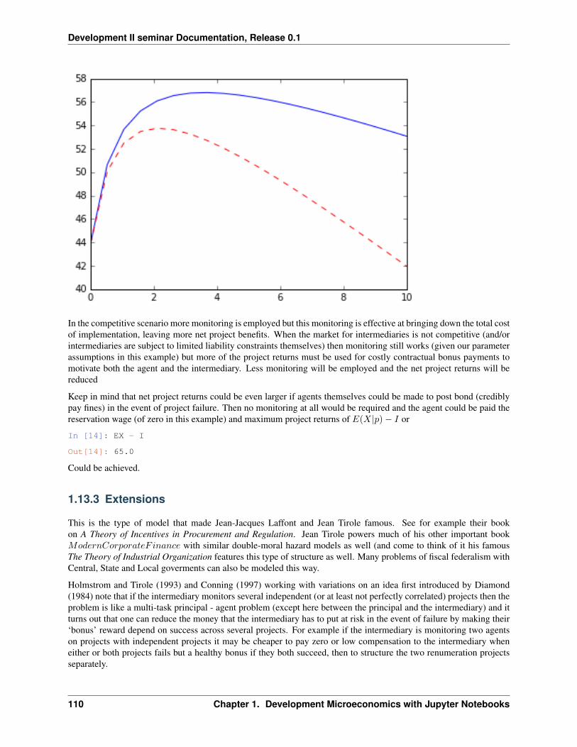
Development II seminar Documentation, Release 0.1
In the competitive scenario more monitoring is employed but this monitoring is effective at bringing down the total costof implementation, leaving more net project benefits. When the market for intermediaries is not competitive (and/orintermediaries are subject to limited liability constraints themselves) then monitoring still works (given our parameterassumptions in this example) but more of the project returns must be used for costly contractual bonus payments tomotivate both the agent and the intermediary. Less monitoring will be employed and the net project returns will bereduced
Keep in mind that net project returns could be even larger if agents themselves could be made to post bond (crediblypay fines) in the event of project failure. Then no monitoring at all would be required and the agent could be paid thereservation wage (of zero in this example) and maximum project returns of 𝐸(𝑋|𝑝) − 𝐼 or
In [14]: EX - I
Out[14]: 65.0
Could be achieved.
1.13.3 Extensions
This is the type of model that made Jean-Jacques Laffont and Jean Tirole famous. See for example their bookon A Theory of Incentives in Procurement and Regulation. Jean Tirole powers much of his other important book𝑀𝑜𝑑𝑒𝑟𝑛𝐶𝑜𝑟𝑝𝑜𝑟𝑎𝑡𝑒𝐹 𝑖𝑛𝑎𝑛𝑐𝑒 with similar double-moral hazard models as well (and come to think of it his famousThe Theory of Industrial Organization features this type of structure as well. Many problems of fiscal federalism withCentral, State and Local goverments can also be modeled this way.
Holmstrom and Tirole (1993) and Conning (1997) working with variations on an idea first introduced by Diamond(1984) note that if the intermediary monitors several independent (or at least not perfectly correlated) projects then theproblem is like a multi-task principal - agent problem (except here between the principal and the intermediary) and itturns out that one can reduce the money that the intermediary has to put at risk in the event of failure by making their‘bonus’ reward depend on success across several projects. For example if the intermediary is monitoring two agentson projects with independent projects it may be cheaper to pay zero or low compensation to the intermediary wheneither or both projects fails but a healthy bonus if they both succeed, then to structure the two renumeration projectsseparately.
110 Chapter 1. Development Microeconomics with Jupyter Notebooks
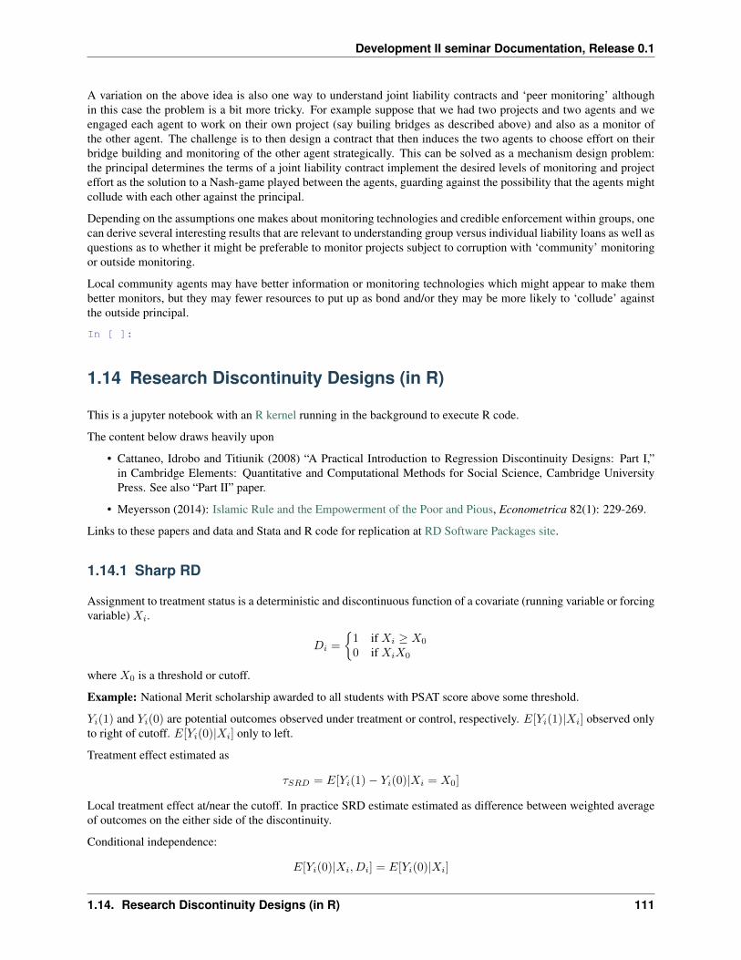
Development II seminar Documentation, Release 0.1
A variation on the above idea is also one way to understand joint liability contracts and ‘peer monitoring’ althoughin this case the problem is a bit more tricky. For example suppose that we had two projects and two agents and weengaged each agent to work on their own project (say builing bridges as described above) and also as a monitor ofthe other agent. The challenge is to then design a contract that then induces the two agents to choose effort on theirbridge building and monitoring of the other agent strategically. This can be solved as a mechanism design problem:the principal determines the terms of a joint liability contract implement the desired levels of monitoring and projecteffort as the solution to a Nash-game played between the agents, guarding against the possibility that the agents mightcollude with each other against the principal.
Depending on the assumptions one makes about monitoring technologies and credible enforcement within groups, onecan derive several interesting results that are relevant to understanding group versus individual liability loans as well asquestions as to whether it might be preferable to monitor projects subject to corruption with ‘community’ monitoringor outside monitoring.
Local community agents may have better information or monitoring technologies which might appear to make thembetter monitors, but they may fewer resources to put up as bond and/or they may be more likely to ‘collude’ againstthe outside principal.
In [ ]:
1.14 Research Discontinuity Designs (in R)
This is a jupyter notebook with an R kernel running in the background to execute R code.
The content below draws heavily upon
• Cattaneo, Idrobo and Titiunik (2008) “A Practical Introduction to Regression Discontinuity Designs: Part I,”in Cambridge Elements: Quantitative and Computational Methods for Social Science, Cambridge UniversityPress. See also “Part II” paper.
• Meyersson (2014): Islamic Rule and the Empowerment of the Poor and Pious, Econometrica 82(1): 229-269.
Links to these papers and data and Stata and R code for replication at RD Software Packages site.
1.14.1 Sharp RD
Assignment to treatment status is a deterministic and discontinuous function of a covariate (running variable or forcingvariable) 𝑋𝑖.
𝐷𝑖 =
{1 if 𝑋𝑖 ≥ 𝑋0
0 if 𝑋𝑖𝑋0
where 𝑋0 is a threshold or cutoff.
Example: National Merit scholarship awarded to all students with PSAT score above some threshold.
𝑌𝑖(1) and 𝑌𝑖(0) are potential outcomes observed under treatment or control, respectively. 𝐸[𝑌𝑖(1)|𝑋𝑖] observed onlyto right of cutoff. 𝐸[𝑌𝑖(0)|𝑋𝑖] only to left.
Treatment effect estimated as
𝜏𝑆𝑅𝐷 = 𝐸[𝑌𝑖(1) − 𝑌𝑖(0)|𝑋𝑖 = 𝑋0]
Local treatment effect at/near the cutoff. In practice SRD estimate estimated as difference between weighted averageof outcomes on the either side of the discontinuity.
Conditional independence:
𝐸[𝑌𝑖(0)|𝑋𝑖, 𝐷𝑖] = 𝐸[𝑌𝑖(0)|𝑋𝑖]
1.14. Research Discontinuity Designs (in R) 111
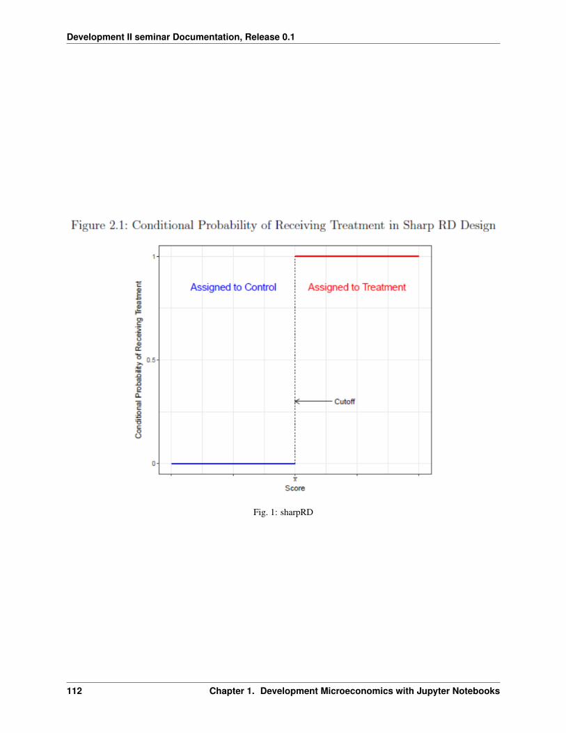
Development II seminar Documentation, Release 0.1
Fig. 1: sharpRD
112 Chapter 1. Development Microeconomics with Jupyter Notebooks
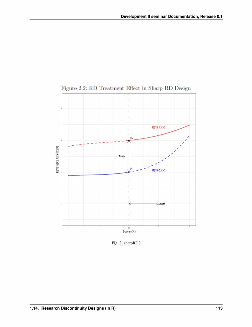
Development II seminar Documentation, Release 0.1
Fig. 2: sharpRD2
1.14. Research Discontinuity Designs (in R) 113
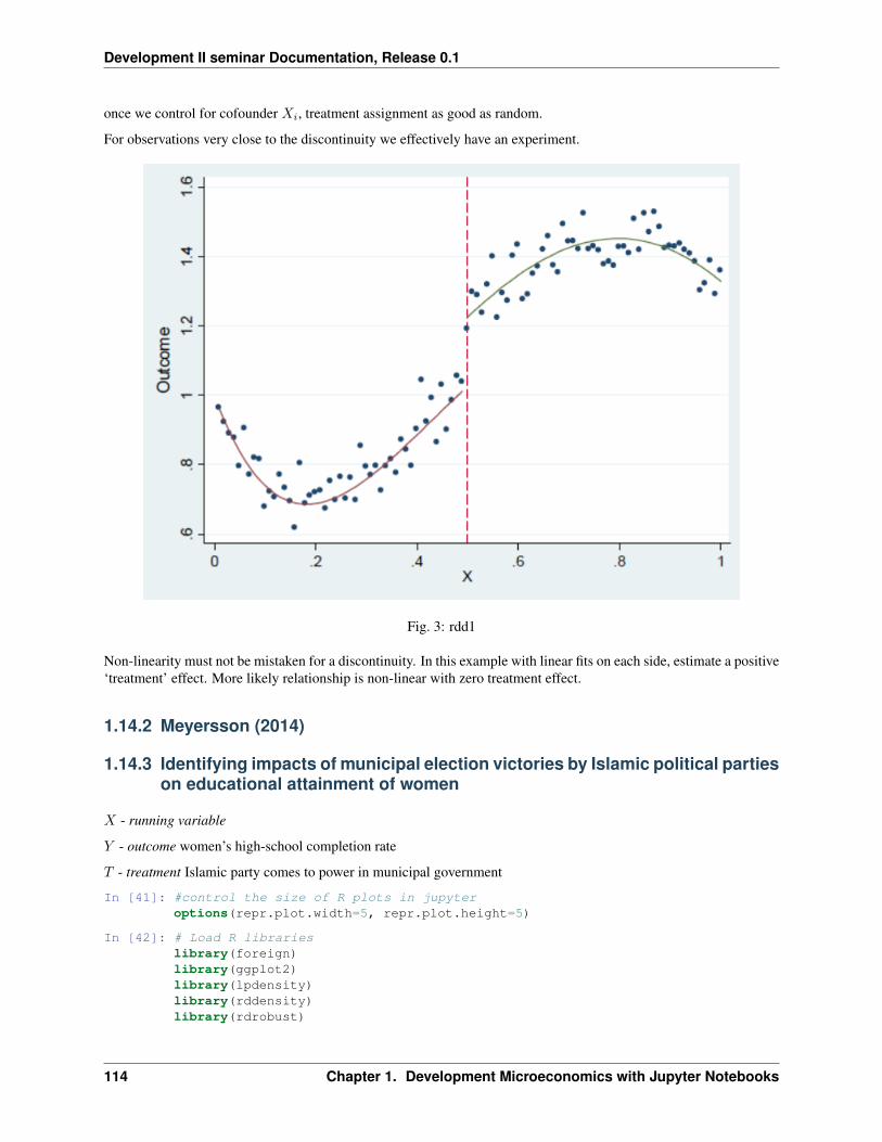
Development II seminar Documentation, Release 0.1
once we control for cofounder 𝑋𝑖, treatment assignment as good as random.
For observations very close to the discontinuity we effectively have an experiment.
Fig. 3: rdd1
Non-linearity must not be mistaken for a discontinuity. In this example with linear fits on each side, estimate a positive‘treatment’ effect. More likely relationship is non-linear with zero treatment effect.
1.14.2 Meyersson (2014)
1.14.3 Identifying impacts of municipal election victories by Islamic political partieson educational attainment of women
𝑋 - running variable
𝑌 - outcome women’s high-school completion rate
𝑇 - treatment Islamic party comes to power in municipal government
In [41]: #control the size of R plots in jupyteroptions(repr.plot.width=5, repr.plot.height=5)
In [42]: # Load R librarieslibrary(foreign)library(ggplot2)library(lpdensity)library(rddensity)library(rdrobust)
114 Chapter 1. Development Microeconomics with Jupyter Notebooks
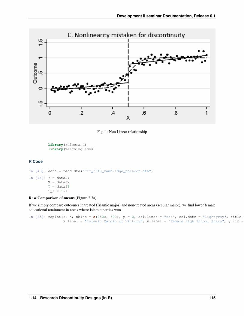
Development II seminar Documentation, Release 0.1
Fig. 4: Non Linear relationship
library(rdlocrand)library(TeachingDemos)
R Code
In [43]: data = read.dta("CIT_2018_Cambridge_polecon.dta")
In [44]: Y = data$YX = data$XT = data$TT_X = T*X
Raw Comparison of means (Figure 2.3a)
If we simply compare outcomes in treated (Islamic major) and non-treated areas (secular major), we find lower femaleeducational attainment in areas where Islamic parties won.
In [45]: rdplot(Y, X, nbins = c(2500, 500), p = 0, col.lines = "red", col.dots = "lightgray", title = "",x.label = "Islamic Margin of Victory", y.label = "Female High School Share", y.lim = c(0,70))
1.14. Research Discontinuity Designs (in R) 115
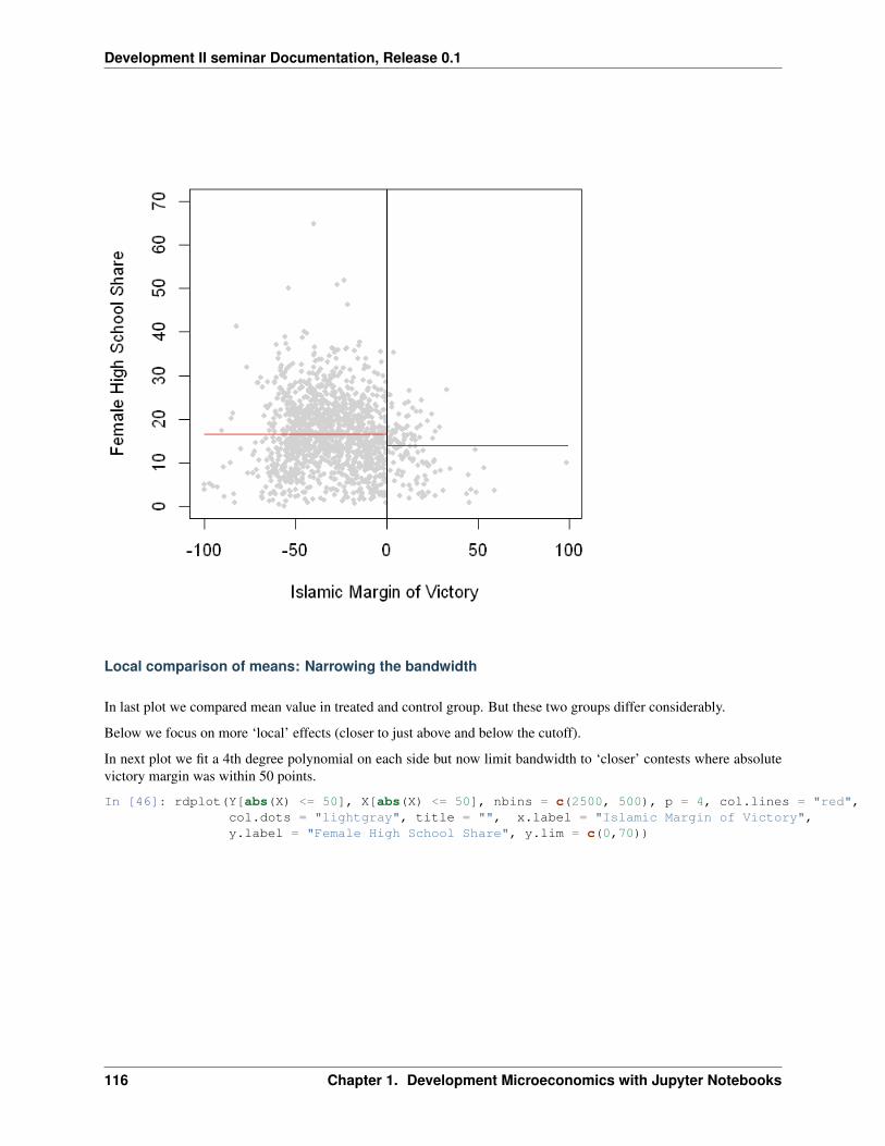
Development II seminar Documentation, Release 0.1
Local comparison of means: Narrowing the bandwidth
In last plot we compared mean value in treated and control group. But these two groups differ considerably.
Below we focus on more ‘local’ effects (closer to just above and below the cutoff).
In next plot we fit a 4th degree polynomial on each side but now limit bandwidth to ‘closer’ contests where absolutevictory margin was within 50 points.
In [46]: rdplot(Y[abs(X) <= 50], X[abs(X) <= 50], nbins = c(2500, 500), p = 4, col.lines = "red",col.dots = "lightgray", title = "", x.label = "Islamic Margin of Victory",y.label = "Female High School Share", y.lim = c(0,70))
116 Chapter 1. Development Microeconomics with Jupyter Notebooks
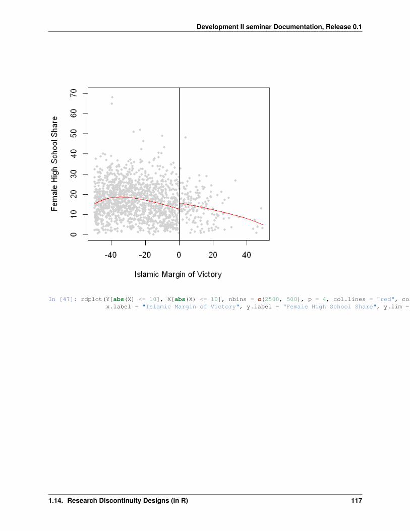
Development II seminar Documentation, Release 0.1
In [47]: rdplot(Y[abs(X) <= 10], X[abs(X) <= 10], nbins = c(2500, 500), p = 4, col.lines = "red", col.dots = "lightgray", title = "",x.label = "Islamic Margin of Victory", y.label = "Female High School Share", y.lim = c(0,70))
1.14. Research Discontinuity Designs (in R) 117
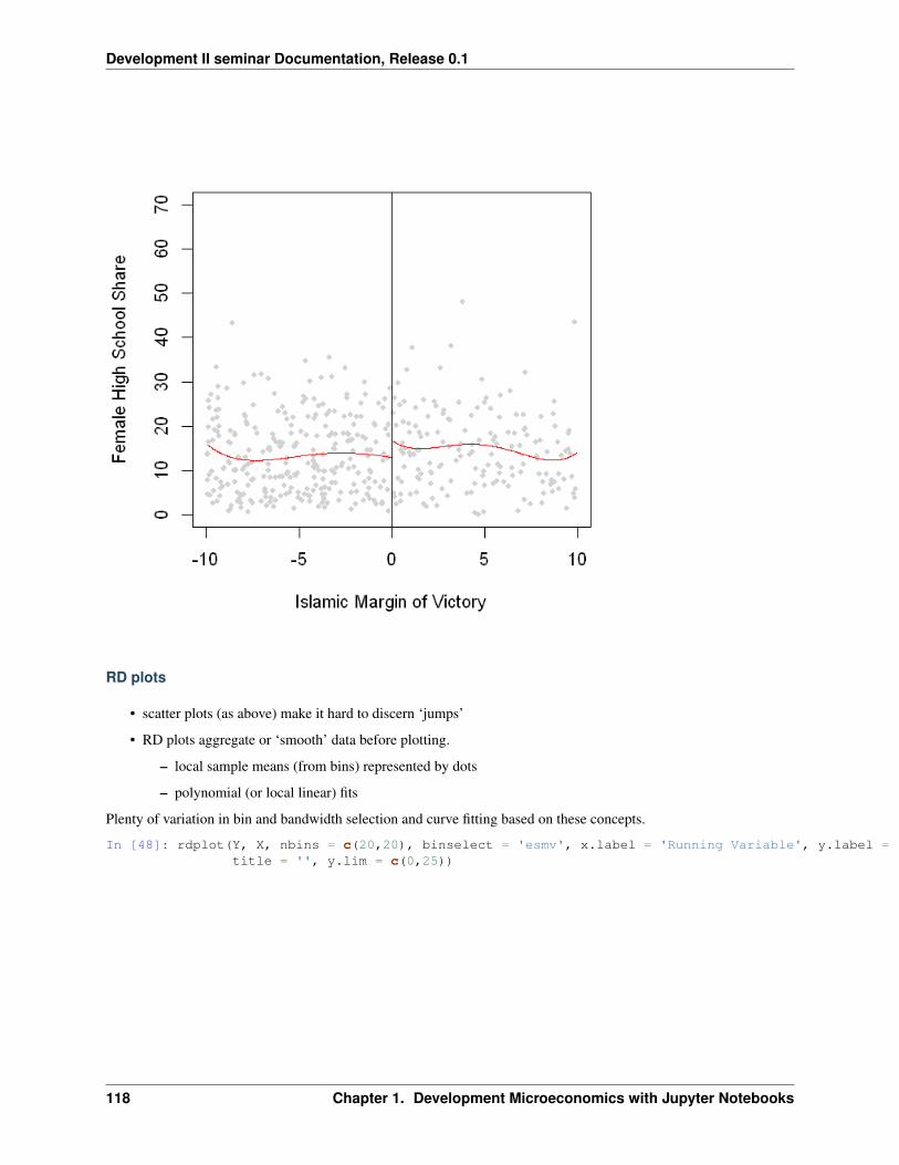
Development II seminar Documentation, Release 0.1
RD plots
• scatter plots (as above) make it hard to discern ‘jumps’
• RD plots aggregate or ‘smooth’ data before plotting.
– local sample means (from bins) represented by dots
– polynomial (or local linear) fits
Plenty of variation in bin and bandwidth selection and curve fitting based on these concepts.
In [48]: rdplot(Y, X, nbins = c(20,20), binselect = 'esmv', x.label = 'Running Variable', y.label = 'Outcome',title = '', y.lim = c(0,25))
118 Chapter 1. Development Microeconomics with Jupyter Notebooks
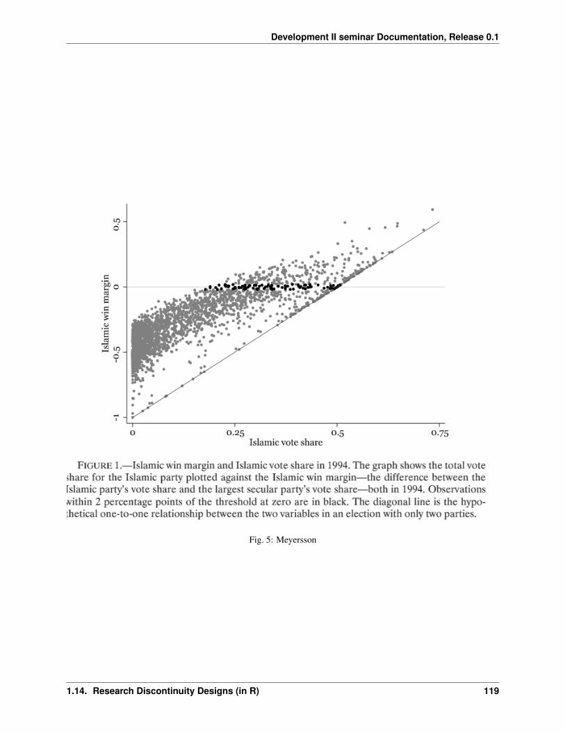
Development II seminar Documentation, Release 0.1
Fig. 5: Meyersson
1.14. Research Discontinuity Designs (in R) 119
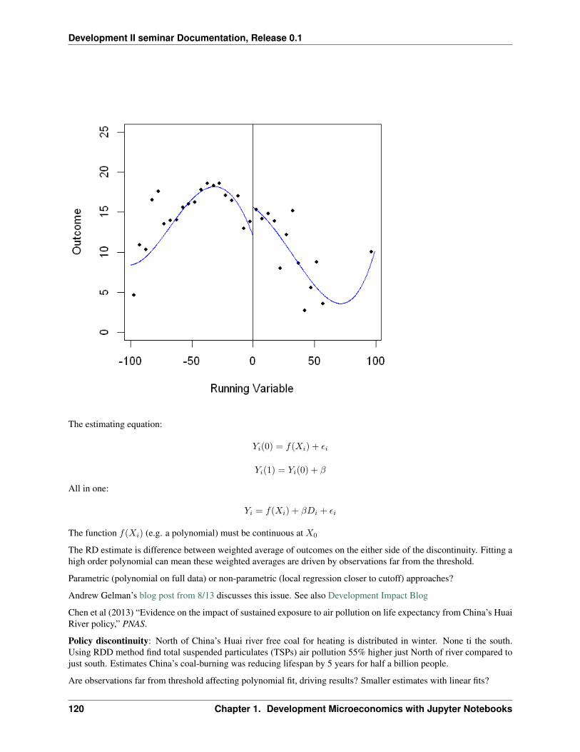
Development II seminar Documentation, Release 0.1
The estimating equation:
𝑌𝑖(0) = 𝑓(𝑋𝑖) + 𝜖𝑖
𝑌𝑖(1) = 𝑌𝑖(0) + 𝛽
All in one:
𝑌𝑖 = 𝑓(𝑋𝑖) + 𝛽𝐷𝑖 + 𝜖𝑖
The function 𝑓(𝑋𝑖) (e.g. a polynomial) must be continuous at 𝑋0
The RD estimate is difference between weighted average of outcomes on the either side of the discontinuity. Fitting ahigh order polynomial can mean these weighted averages are driven by observations far from the threshold.
Parametric (polynomial on full data) or non-parametric (local regression closer to cutoff) approaches?
Andrew Gelman’s blog post from 8/13 discusses this issue. See also Development Impact Blog
Chen et al (2013) “Evidence on the impact of sustained exposure to air pollution on life expectancy from China’s HuaiRiver policy,” PNAS.
Policy discontinuity: North of China’s Huai river free coal for heating is distributed in winter. None ti the south.Using RDD method find total suspended particulates (TSPs) air pollution 55% higher just North of river compared tojust south. Estimates China’s coal-burning was reducing lifespan by 5 years for half a billion people.
Are observations far from threshold affecting polynomial fit, driving results? Smaller estimates with linear fits?
120 Chapter 1. Development Microeconomics with Jupyter Notebooks
Development II seminar Documentation, Release 0.1
notebooks/images/ChinaRDD.png
notebooks/images/ChinaRDD2.PNG
Fuzzy RD
notebooks/images/fuzzy.PNG
A fuzzy RD is like an RD with imperfect compliance or non-compliance. Assignment to Treatment is as beforesummarized by indicator 𝐼(𝑋𝑖 ≥ 𝑋0) but compliance is now imperfect. Like an Intent-to-Treat (ITT) estimator, themeasured jump at the cutoff in the outcome needs to be rescaled.
Structural equation: 𝑌𝑖 = 𝑓(𝑋𝑖) + 𝛽𝐷𝑖 + 𝜖𝑖
2nd stage reduced form: 𝑌𝑖 = 𝑓(𝑋𝑖) + 𝜋2𝐼(𝑋𝑖 ≥ 𝑋0 + 𝜉2𝑖
First stage: 𝐷𝑖 = 𝑔(𝑋𝑖) + 𝜋1𝐼(𝑋𝑖 ≥ 𝑋0 + 𝜉1𝑖
Standard IV: $ 𝛽 =
Multi-Score RD design
Example: Third graders have to go to summer school if score below 𝑋10 in reading test OR below 𝑋20 in math test.Does summer school raise test performance next year?
notebooks/images/2d_distance.PNG
From Zamosc 2012
1.14.4 Polynomial Fit in 2 dimensions
With two forcing variables - The cutoff is now a boundary - Heterogenous effects, depending on what segment ofthe boundary - with right assumptions (lots of data), can identify one treatment effect for every point b on boundary.Treatment effect curve 𝜏(𝑏) - Average Treatment Effect (ATE) would average over boundary
1.14. Research Discontinuity Designs (in R) 121
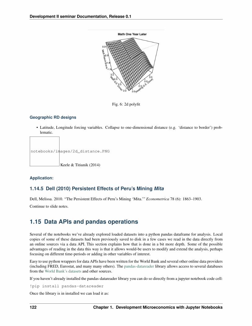
Development II seminar Documentation, Release 0.1
Fig. 6: 2d polyfit
Geographic RD designs
• Latitude, Longitude forcing variables. Collapse to one-dimensional distance (e.g. ‘distance to border’) prob-lematic.
notebooks/images/2d_distance.PNG
Keele & Titiunik (2014)
Application:
1.14.5 Dell (2010) Persistent Effects of Peru’s Mining Mita
Dell, Melissa. 2010. “The Persistent Effects of Peru’s Mining ‘Mita.’” Econometrica 78 (6): 1863–1903.
Continue to slide notes.
1.15 Data APIs and pandas operations
Several of the notebooks we’ve already explored loaded datasets into a python pandas dataframe for analysis. Localcopies of some of these datasets had been previously saved to disk in a few cases we read in the data directly froman online sources via a data API. This section explains how that is done in a bit more depth. Some of the possibleadvantages of reading in the data this way is that it allows would-be users to modify and extend the analysis, perhapsfocusing on different time-periods or adding in other variables of interest.
Easy to use python wrappers for data APIs have been written for the World Bank and several other online data providers(including FRED, Eurostat, and many many others). The pandas-datareader library allows access to several databasesfrom the World Bank’s datasets and other sources.
If you haven’t already installed the pandas-datareader library you can do so directly from a jupyter notebook code cell:
!pip install pandas-datareader
Once the library is in installed we can load it as:
122 Chapter 1. Development Microeconomics with Jupyter Notebooks
Development II seminar Documentation, Release 0.1
In [1]: %matplotlib inlineimport seaborn as snsimport warningsimport numpy as npimport statsmodels.formula.api as smfimport datetime as dt
In [2]: from pandas_datareader import wb
1.15.1 Data on urban bias
Our earlier analysis of the Harris_Todaro migration model suggested that policies designed to favor certain sectors orlabor groups
Let’s search for indicators (and their identification codes) relating to GDP per capita and urban population share. Wecould look these up in a book or from the website http://data.worldbank.org/ but we can also search for keywordsdirectly.
First lets search for series having to do with gdp per capita
In [3]: wb.search('gdp.*capita.*const')[['id','name']]
Out[3]: id name685 6.0.GDPpc_constant GDP per capita, PPP (constant 2011 internation...7588 NY.GDP.PCAP.KD GDP per capita (constant 2010 US$)7590 NY.GDP.PCAP.KN GDP per capita (constant LCU)7592 NY.GDP.PCAP.PP.KD GDP per capita, PPP (constant 2011 internation...
We will use NY.GDP.PCAP.KD for GDP per capita (constant 2010 US$).
You can also first browse and search for data series from the World Bank’s DataBank page at http://databank.worldbank.org/data/. Then find the ‘id’ for the series that you are interested in in the ‘metadata’ section from thewebpage
Now let’s look for data on urban population share:
In [4]: wb.search('Urban Population')[['id','name']].tail()
Out[4]: id name9999 SP.URB.GROW Urban population growth (annual %)10000 SP.URB.TOTL Urban population10001 SP.URB.TOTL.FE.ZS Urban population, female (% of total)10002 SP.URB.TOTL.IN.ZS Urban population (% of total)10003 SP.URB.TOTL.MA.ZS Urban population, male (% of total)
Let’s use the ones we like but use a python dictionary to rename these to shorter variable names when we load the datainto a python dataframe:
In [5]: indicators = ['NY.GDP.PCAP.KD', 'SP.URB.TOTL.IN.ZS']
Since we are interested in exploring the extent of ‘urban bias’ in some countries, let’s load data from 1980 which wastoward the end of the era of import-substituting industrialization when urban-biased policies were claimed to be mostpronounced.
In [6]: dat = wb.download(indicator=indicators, country = 'all', start=1980, end=1980)
In [7]: dat.columns
Out[7]: Index(['NY.GDP.PCAP.KD', 'SP.URB.TOTL.IN.ZS'], dtype='object')
Let’s rename the columns to something shorter and then plot and regress log gdp per capita against urban extent weget a pretty tight fit:
1.15. Data APIs and pandas operations 123
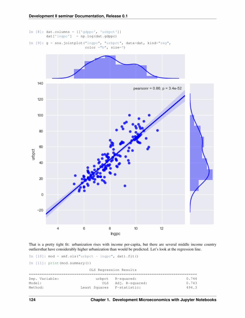
Development II seminar Documentation, Release 0.1
In [8]: dat.columns = [['gdppc', 'urbpct']]dat['lngpc'] = np.log(dat.gdppc)
In [9]: g = sns.jointplot("lngpc", "urbpct", data=dat, kind="reg",color ="b", size=7)
That is a pretty tight fit: urbanization rises with income per-capita, but there are several middle income countryoutliersthat have considerably higher urbanization than would be predicted. Let’s look at the regression line.
In [10]: mod = smf.ols("urbpct ~ lngpc", dat).fit()
In [11]: print(mod.summary())
OLS Regression Results==============================================================================Dep. Variable: urbpct R-squared: 0.744Model: OLS Adj. R-squared: 0.743Method: Least Squares F-statistic: 494.3
124 Chapter 1. Development Microeconomics with Jupyter Notebooks
Development II seminar Documentation, Release 0.1
Date: Wed, 03 May 2017 Prob (F-statistic): 3.43e-52Time: 15:26:52 Log-Likelihood: -670.94No. Observations: 172 AIC: 1346.Df Residuals: 170 BIC: 1352.Df Model: 1Covariance Type: nonrobust==============================================================================
coef std err t P>|t| [0.025 0.975]------------------------------------------------------------------------------Intercept -68.0209 5.185 -13.120 0.000 -78.255 -57.787lngpc 13.9583 0.628 22.233 0.000 12.719 15.198==============================================================================Omnibus: 8.555 Durbin-Watson: 2.204Prob(Omnibus): 0.014 Jarque-Bera (JB): 17.062Skew: -0.027 Prob(JB): 0.000197Kurtosis: 4.542 Cond. No. 47.3==============================================================================
Warnings:[1] Standard Errors assume that the covariance matrix of the errors is correctly specified.
Now let’s just look at a list of countries sorted by the size of their residuals in this regression line. Countries with thelargest residuals had urbanization in excess of what the model predicts from their 1980 level of income per capita.
Here is the sorted list of top 15 outliers.
In [12]: mod.resid.sort_values(ascending=False).head(15)
Out[12]: country yearSingapore 1980 35.469714Chile 1980 30.563014Malta 1980 30.448467Hong Kong SAR, China 1980 29.957702Uruguay 1980 29.143223Argentina 1980 25.369855Cuba 1980 24.148529Belgium 1980 20.731859Israel 1980 20.456625Iraq 1980 20.262678Peru 1980 17.810693Myanmar 1980 17.719561Bulgaria 1980 17.360914Jordan 1980 15.706878Colombia 1980 15.258744dtype: float64
This is of course only suggestive but (leaving aside the island states like Singapore and Hong-Kong) the list is dom-inated by southern cone countries such as Chile, Argentina and Peru which in addition to having legacies of heavypolitical centralization also pursued ISI policies in the 60s and 70s that many would associate with urban biasedpolicies.
Panel data
Very often we want data on several indicators and a whole group of countries over a number of years. we could alsohave used datetime format dates:
In [13]: countries = ['CHL', 'USA', 'ARG']start, end = dt.datetime(1950, 1, 1), dt.datetime(2016, 1, 1)dat = wb.download(
indicator=indicators,
1.15. Data APIs and pandas operations 125
Development II seminar Documentation, Release 0.1
country = countries,start=start,end=end).dropna()
Lets use shorter column names
In [14]: dat.columns
Out[14]: Index(['NY.GDP.PCAP.KD', 'SP.URB.TOTL.IN.ZS'], dtype='object')
In [15]: dat.columns = [['gdppc', 'urb']]
In [16]: dat.head()
Out[16]: gdppc urbcountry yearArgentina 2015 10501.660269 91.751
2014 10334.780146 91.6042013 10711.229530 91.4522012 10558.265365 91.2952011 10780.342508 91.133
Notice this has a two-level multi-index. The outer level is named ‘country’ and the inner level is ‘year’
We can pull out group data for a single country like this using the .xs or cross section method.
In [17]: dat.xs('Chile',level='country').head(3)
Out[17]: gdppc urbyear2015 14660.505335 89.5302014 14479.763258 89.3562013 14364.140970 89.175
(Note we could have also used dat.loc['Chile'].head())
And we can pull a ‘year’ level cross section like this:
In [18]: dat.xs('2007', level='year').head()
Out[18]: gdppc urbcountryArgentina 9830.759871 90.445Chile 12223.484611 87.926United States 49979.533843 80.269
Note that what was returned was a dataframe with the data just for our selected country. We can in turn further specifywhat column(s) from this we want:
In [19]: dat.loc['Chile']['gdppc'].head()
Out[19]: year2015 14660.5053352014 14479.7632582013 14364.1409702012 13963.6654022011 13385.131216Name: gdppc, dtype: float64
Unstack data
The unstack method turns index values into column names while stack method converts column names to index values.Here we apply unstack.
126 Chapter 1. Development Microeconomics with Jupyter Notebooks
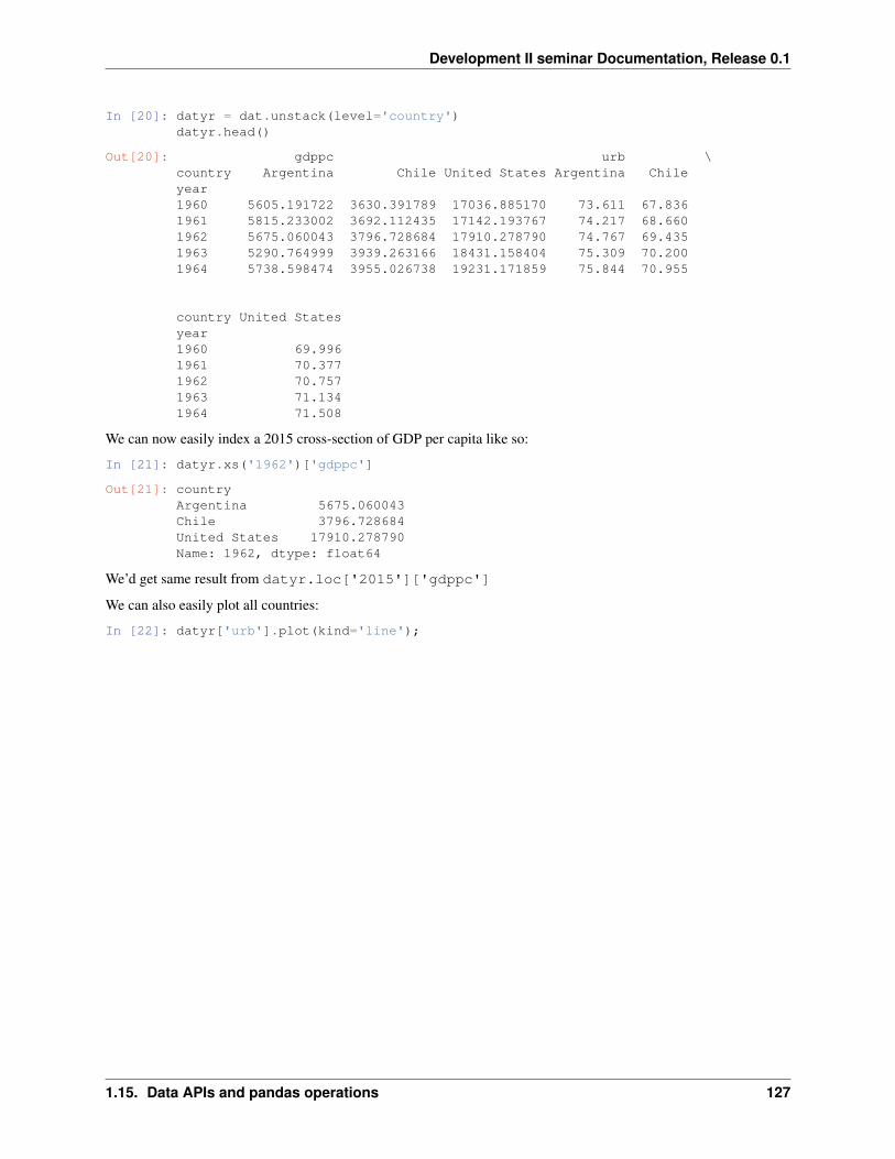
Development II seminar Documentation, Release 0.1
In [20]: datyr = dat.unstack(level='country')datyr.head()
Out[20]: gdppc urb \country Argentina Chile United States Argentina Chileyear1960 5605.191722 3630.391789 17036.885170 73.611 67.8361961 5815.233002 3692.112435 17142.193767 74.217 68.6601962 5675.060043 3796.728684 17910.278790 74.767 69.4351963 5290.764999 3939.263166 18431.158404 75.309 70.2001964 5738.598474 3955.026738 19231.171859 75.844 70.955
country United Statesyear1960 69.9961961 70.3771962 70.7571963 71.1341964 71.508
We can now easily index a 2015 cross-section of GDP per capita like so:
In [21]: datyr.xs('1962')['gdppc']
Out[21]: countryArgentina 5675.060043Chile 3796.728684United States 17910.278790Name: 1962, dtype: float64
We’d get same result from datyr.loc['2015']['gdppc']
We can also easily plot all countries:
In [22]: datyr['urb'].plot(kind='line');
1.15. Data APIs and pandas operations 127
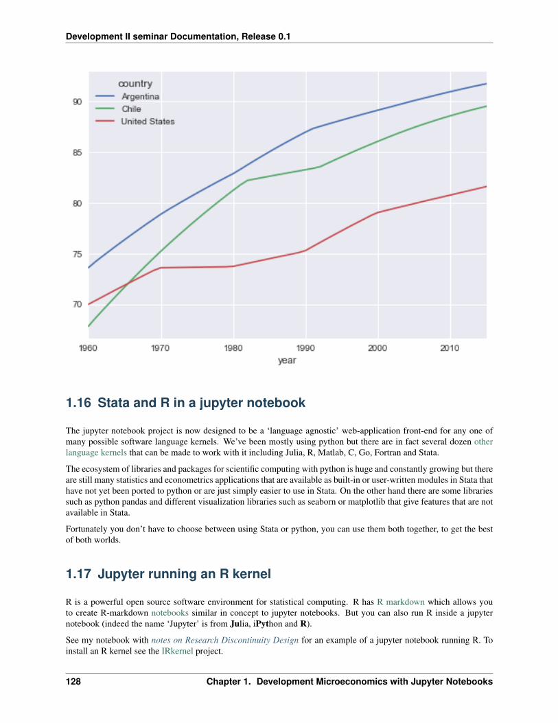
Development II seminar Documentation, Release 0.1
1.16 Stata and R in a jupyter notebook
The jupyter notebook project is now designed to be a ‘language agnostic’ web-application front-end for any one ofmany possible software language kernels. We’ve been mostly using python but there are in fact several dozen otherlanguage kernels that can be made to work with it including Julia, R, Matlab, C, Go, Fortran and Stata.
The ecosystem of libraries and packages for scientific computing with python is huge and constantly growing but thereare still many statistics and econometrics applications that are available as built-in or user-written modules in Stata thathave not yet been ported to python or are just simply easier to use in Stata. On the other hand there are some librariessuch as python pandas and different visualization libraries such as seaborn or matplotlib that give features that are notavailable in Stata.
Fortunately you don’t have to choose between using Stata or python, you can use them both together, to get the bestof both worlds.
1.17 Jupyter running an R kernel
R is a powerful open source software environment for statistical computing. R has R markdown which allows youto create R-markdown notebooks similar in concept to jupyter notebooks. But you can also run R inside a jupyternotebook (indeed the name ‘Jupyter’ is from Julia, iPython and R).
See my notebook with notes on Research Discontinuity Design for an example of a jupyter notebook running R. Toinstall an R kernel see the IRkernel project.
128 Chapter 1. Development Microeconomics with Jupyter Notebooks
Development II seminar Documentation, Release 0.1
1.18 Jupyter with a Stata Kernel
Kyle Barron has created a stata_kernel that offers several useful features including code-autocompletion, inline graph-ics, and generally fast responses.
For this to work you must have a working licensed copy of Stata version 14 or greater on your machine.
1.19 Python and Stata combined in the same notebook
Sometimes it may be useful to combine python and Stata in the same notebook. Ties de Kok has written a nice pythonlibrary called ipystata that allows one to execute Stata code in codeblocks inside an ipython notebook when precededby a %%stata magic command.
This workflow allows you to pass data between python and Stata sessions and to display Stata plots inline. Comparedto the stata_kernel option the response times are not quite as fast.
The remainder of this notebook illustrates the use of ipystata.
1.19.1 A sample ipystata session
For more details see the example notebook and documentation on the ipystata repository.
In [1]: %matplotlib inlineimport seaborn as snsimport pandas as pdimport statsmodels.formula.api as smfimport ipystata
The following opens a Stata session where we load a dataset and summarize the data. The -o flag following the‘%%Stata‘‘‘ magic instructs it to output or return the dataset in Stata memory as a pandas dataframe in python.
In [2]: %%stata -o life_dfsysuse lifeexp.dtasummarize
(Life expectancy, 1998)
Variable | Obs Mean Std. Dev. Min Max-------------+---------------------------------------------------------
region | 68 1.5 .7431277 1 3country | 0
popgrowth | 68 .9720588 .9311918 -.5 3lexp | 68 72.27941 4.715315 54 79
gnppc | 63 8674.857 10634.68 370 39980-------------+---------------------------------------------------------
safewater | 40 76.1 17.89112 28 100
Let’s confirm the data was returned as a pandas dataframe:
In [3]: life_df.head(3)
Out[3]: region country popgrowth lexp gnppc safewater0 Eur & C.Asia Albania 1.2 72 810.0 76.01 Eur & C.Asia Armenia 1.1 74 460.0 NaN2 Eur & C.Asia Austria 0.4 79 26830.0 NaN
1.18. Jupyter with a Stata Kernel 129
Development II seminar Documentation, Release 0.1
A simple generate variable command and ols regression in Stata:
In [4]: %%stata -o life_dfgen lngnppc = ln(gnppc)regress lexp lngnppc
(5 missing values generated)
Source | SS df MS Number of obs = 63-------------+---------------------------------- F(1, 61) = 97.09
Model | 873.264865 1 873.264865 Prob > F = 0.0000Residual | 548.671643 61 8.99461709 R-squared = 0.6141
-------------+---------------------------------- Adj R-squared = 0.6078Total | 1421.93651 62 22.9344598 Root MSE = 2.9991
------------------------------------------------------------------------------lexp | Coef. Std. Err. t P>|t| [95% Conf. Interval]
-------------+----------------------------------------------------------------lngnppc | 2.768349 .2809566 9.85 0.000 2.206542 3.330157
_cons | 49.41502 2.348494 21.04 0.000 44.71892 54.11113------------------------------------------------------------------------------
And the same regression using statsmodels and pandas:
In [5]: model = smf.ols(formula = 'lexp ~ lngnppc',data = life_df)
results = model.fit()print(results.summary())
OLS Regression Results==============================================================================Dep. Variable: lexp R-squared: 0.614Model: OLS Adj. R-squared: 0.608Method: Least Squares F-statistic: 97.09Date: Tue, 08 May 2018 Prob (F-statistic): 3.13e-14Time: 14:25:48 Log-Likelihood: -157.57No. Observations: 63 AIC: 319.1Df Residuals: 61 BIC: 323.4Df Model: 1Covariance Type: nonrobust==============================================================================
coef std err t P>|t| [0.025 0.975]------------------------------------------------------------------------------Intercept 49.4150 2.348 21.041 0.000 44.719 54.111lngnppc 2.7683 0.281 9.853 0.000 2.207 3.330==============================================================================Omnibus: 21.505 Durbin-Watson: 1.518Prob(Omnibus): 0.000 Jarque-Bera (JB): 46.140Skew: -1.038 Prob(JB): 9.57e-11Kurtosis: 6.643 Cond. No. 52.7==============================================================================
Warnings:[1] Standard Errors assume that the covariance matrix of the errors is correctly specified.
Back to ipython
Let’s change one of the variables in the dataframe in python:
130 Chapter 1. Development Microeconomics with Jupyter Notebooks
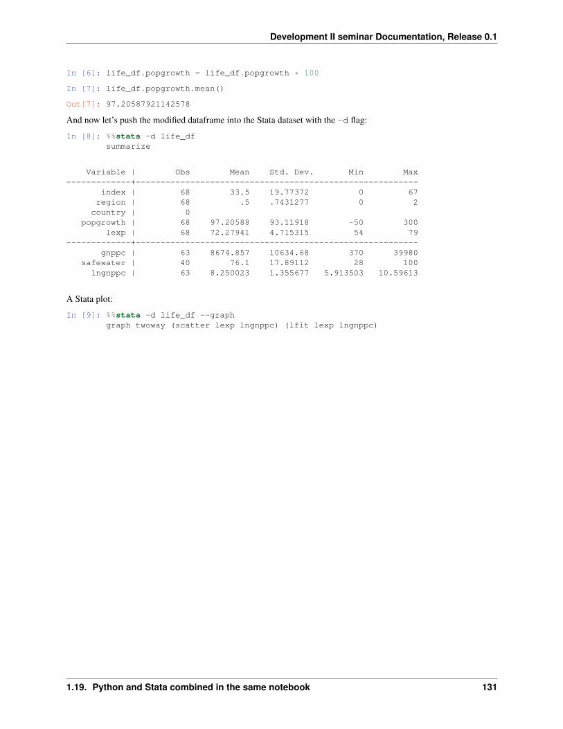
Development II seminar Documentation, Release 0.1
In [6]: life_df.popgrowth = life_df.popgrowth * 100
In [7]: life_df.popgrowth.mean()
Out[7]: 97.20587921142578
And now let’s push the modified dataframe into the Stata dataset with the -d flag:
In [8]: %%stata -d life_dfsummarize
Variable | Obs Mean Std. Dev. Min Max-------------+---------------------------------------------------------
index | 68 33.5 19.77372 0 67region | 68 .5 .7431277 0 2
country | 0popgrowth | 68 97.20588 93.11918 -50 300
lexp | 68 72.27941 4.715315 54 79-------------+---------------------------------------------------------
gnppc | 63 8674.857 10634.68 370 39980safewater | 40 76.1 17.89112 28 100
lngnppc | 63 8.250023 1.355677 5.913503 10.59613
A Stata plot:
In [9]: %%stata -d life_df --graphgraph twoway (scatter lexp lngnppc) (lfit lexp lngnppc)
1.19. Python and Stata combined in the same notebook 131
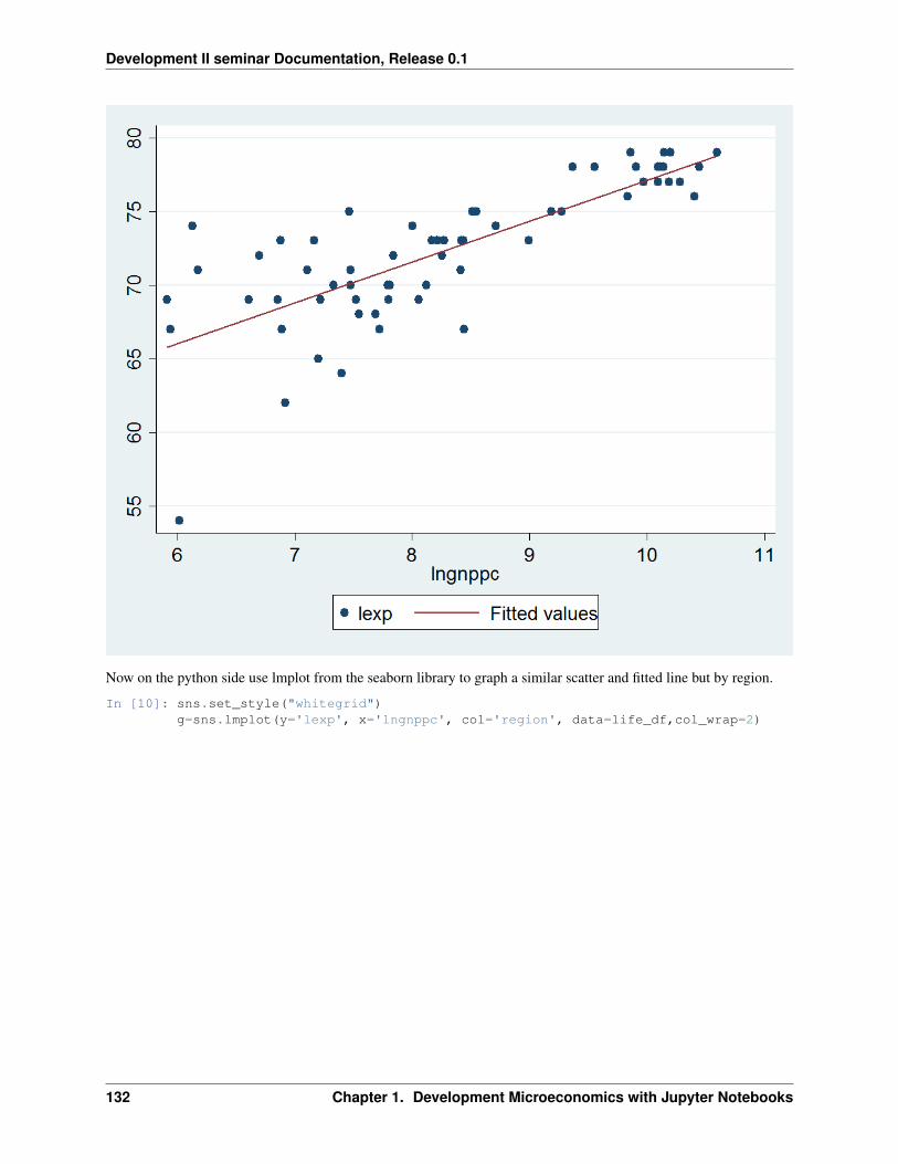
Development II seminar Documentation, Release 0.1
Now on the python side use lmplot from the seaborn library to graph a similar scatter and fitted line but by region.
In [10]: sns.set_style("whitegrid")g=sns.lmplot(y='lexp', x='lngnppc', col='region', data=life_df,col_wrap=2)
132 Chapter 1. Development Microeconomics with Jupyter Notebooks
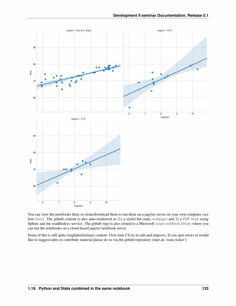
Development II seminar Documentation, Release 0.1
You can view the notebooks there or clone/download them to run them on a jupyter server on your own computer (seehow here). The github content is also auto-rendeered as (1) a styled but static webpages and 2) a PDF book usingSphinx and the readthedocs service. The github repo is also cloned to a Microsoft Azure notebook library where youcan run the notebooks on a cloud-based jupyter notebook server.
Some of this is still quite rough/preliminary content. Over time I’ll try to edit and improve. If you spot errors or wouldlike to suggest edits or contribute material please do so via the github repository (start an ‘issue ticket’):
1.19. Python and Stata combined in the same notebook 133