digital comms -tutorial- parte i

IEEE COMMUNICATIONS MAGAZINE

A Structured Overview of Digital Communications-a Tutorialu Review-Part I BERNARD SKLAR

Part I of a two-part overview of digital communications.

A N IMPRESSIVE assortment of communications signal processing techniques has arisen during the past two decades. This two-part paper presents an

overview of some of these techniques, particularly as they relate to digital satellite communications. The material is developed in the context of a structure used to trace the processing steps from the information source to the information sink. Transformations are organized according to functional classes: formatting and source coding, modulation, channel coding, multiplexing and multiple access, frequency spreading, encryption, and synchronization. The paper begins by treating formatting, source coding, modulation, and potential trade-offs for power-limited systems ' and bandwidth-limited systems.

Communications via satellites have two unique characteristics: the ability to cover the globe with a flexibility that cannot be duplicated with terrestrial links, and the availability of bandwidth exceeding anything previously available for intercontinental communications [ 11. Most satellite communications systems to date have been analog in nature. However, digital communications is becoming increasingly attractive because of the ever-growing demand for data communication, and because digital transmission offers data processing options and flexibilities not available with analog transmission [2].

This paper presents an overview of digital communications in general; for the most part, however, the treatment is in the context of a satellite communications link. The key feature of a digital communications system (DCS) is that it sends only a finite set of messages, in contrast to an analog communications system, which can send an infinite set of messages. In a DCS, the objective at the receiver is not to reproduce a waveform with precision; it is instead to determine from a noise-perturbed signal which of the finite set of waveforms had been sent by the transmitter. An important measure of system performance is the average number of erroneous decisions made, or the probability of error ( P E ) .

Figure 1 illustrates a typical DCS. Let there be M symbols or messages ml , m2, . , . , mM to be transmitted. Let each

symbol be represented by transmitting a corresponding waveformsl(t),s2(t), . . . , sM(t).Thesymbol(ormessage) mi is sent by transmitting the digital waveform s i ( t ) for T seconds, the symbol period. The next symbol is sent over the next period. Since the M symbols can be represented by k = log2M binary digits (bits), the data rate can be expressed as

R = ( l / T ) log,M = k/T b/s. Data rate is usually expressed in bits per second (b/s) whether or not binary digits are actually involved. A binary symbol is the special case characterized by M = 2 and k = 1. A digital waveform is taken to mean a voltage or current waveform representing a digital symbol. The waveform is endowed with specially chosen amplitude, frequency, or phase characteristics that allow the selection of a distinct-waveform for each symbol from a finite set of symbols. At various points along the signal route, noise corrupts the waveforms s( t ) so that its reception must be termed an estimate i(t). Such noise, and its deleterious effect on system performance, will be treated in Part I1 of this paper, which will appear in the October 1983 IEEE Communications Magazine.

Signal Processing Steps

. .

The functional block diagram shown in Fig. 1 illustrates the data flow through the DCS. The upper blocks, which are labeled format, source encode, encrypt, channel encode, multiplex, modulate, frequency spread, and multiple access, dictate the signal transformations from the source to the transmitter. The lower blocks dictate the signal transformations from the receiver back to the source; the lower blocks essentially reverse the signal processing steps performed by the upper blocks. The blocks within the dashed lines initially consisted only of the modulator and demodulator functions, hence the name MODEM. During the past two decades, other signal processing functions were frequently incorporated within the same assembly as the modulator and dem.odulator. Consequently, the term MODEM often encompasses the processing steps shown within the dashed lines of Fig. 1. When this is the case, the MODEM can be thought of as the

0163-6804/83/0800-0004$01 .OO 0 1983 IEEE

AUGUST 1983

“brains” of the system, and the transmitter and receiver as the “muscles.” While the transmitter^ ,consists of a frequency up-conversion stage, a high-power amplifier, and an antenna, the receiver portion is occupied by an antenna, a low-noise front-end amplifier, and a down-converter stage, typically to an intermediate frequency (IF).

Of all the signal processing steps, only formatting, modulation, and demodulation are essential for all DCS’s; the other processing steps within the MODEM are considered design options for various system needs. Source encoding, as defined here, removes information redundancy and performs analog-to-digital (A/D) conversion. Encryption prevents unauthorized users from understanding messages and from injecting false messages into the system. Channel coding can, for a given data rate, improve the PE performance at the expense of power or bandwidth, reduce the system bandwidth requirement at the expense of power o r PE performance, or reduce the power requirement at the expense of bandwidth or PE performance. Frequency spreading renders the signal less vulnerable to interference (both natural and intentional) and can be used to afford privacy to the communicators. Multiplexing and multiple access combine signals that might have different characteristics or originate from different, sources.

The flow of the signal processing steps shown in Fig. 1 represents a typical arrangement; however, the blocks are sometimes implemented in a different order. For example, multiplexing can take place prior to channel encoding,

prior to modulation, or-with a two-step modulation process (subcarrier and carrier)-it can be performed between the two steps. Similarly, spreading can take place anywhere along the transmission chain; its precise location depends on the particular technique used. Figure 1 illustrates the reciprocal aspect of the procedure; any signal processing steps which take place in the transmitting chain must be reversed in the receiving chain. The figure also indicates that, from the source to the modulator, a message takes the form of a bit stream, also called a baseband signal. After modulation, the message takes the form of a digitally encoded sinusoid (digital waveform). Similarly, in the reverse direction, a received message appears as a digital waveform until it is demodu- lated. Thereafter it takes the form of a bit stream for all further signal processing steps.

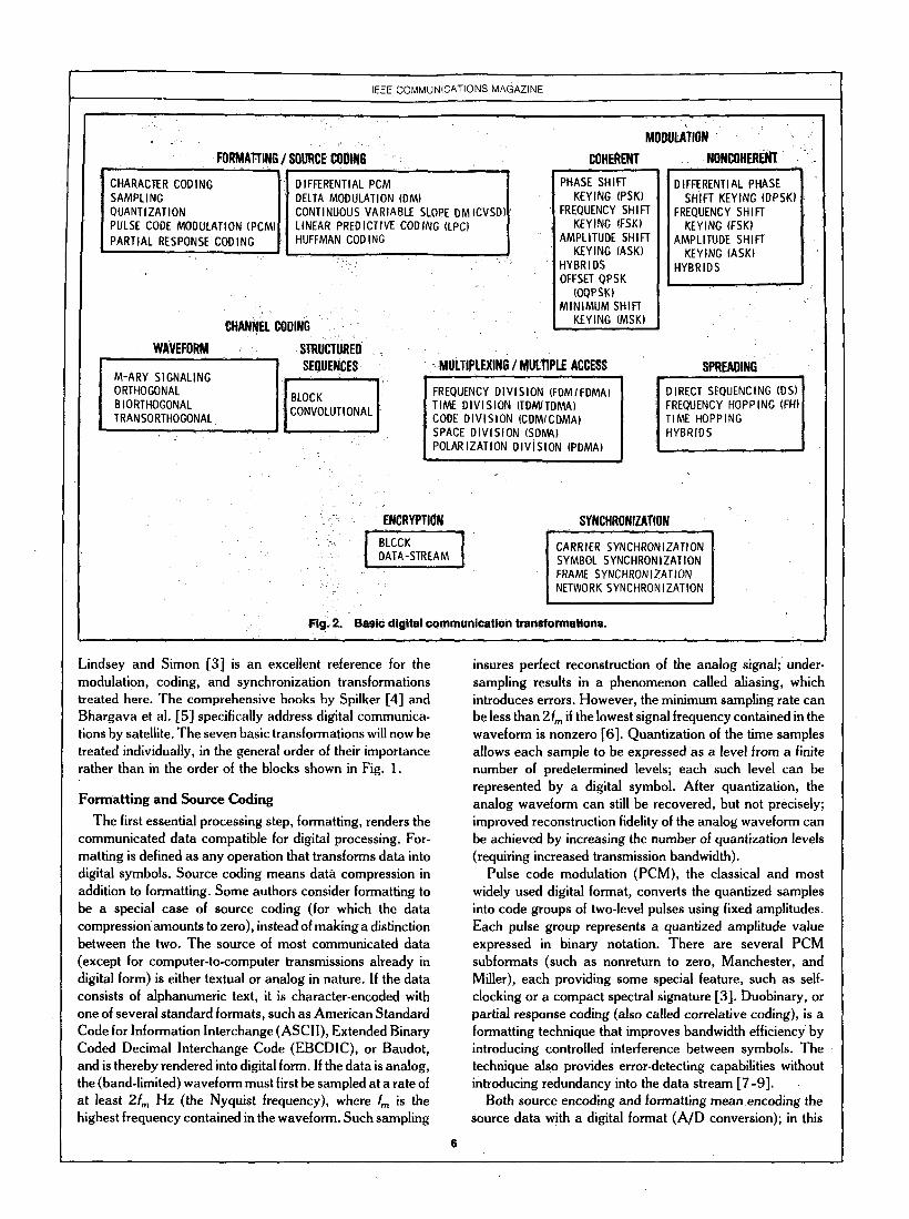
Figure 2 shows the basic signal processing functions, which may be viewed as transformations from one signal space to another. The transformations are classified into seven basic groups:

0 formatting and source coding 0 modulation 0 channel coding

multiplexing and multiple access 0 spreading 0 encryption 0 synchronization The organization has some inherent overlap, but neverthe-

less provides a useful structure for this overview. The text by

INFORMATION I SOURCE I SINK BITS I

OPTIONAL L - - - - - - ---- - ---------_ J 0 ESSENTIAL T 3 OTHER DESTINATIONS

I Fig. 1. Block diagram of a typical digital communication system.

5

FORMARING / SOURCE COOING COHERENT

CHARACTER CODING SAMPLING DELTA MODULATION (DM) QUANTIZATION CONTINUOUS VARIABLE SLOPE D M (CVSD)

PARTIAL RESPONSE CODING HUFFMAN CODING

r

x , . , ' ' . I )

. .

CHANNEL CODING '

.

. .

M-ARY SIGNALING ORTHOGONAL BIORTHOGONAL TRANSORTHOGONAL

SEaUEMCES .MULTIPLEXING / MULTIPLE ACCESS

BLOCK CONVOLUTIONAL

MODUU\TION

PHASE SHIFT KEYING (PSK)

FREQUENCY SHIFT KEYING (FSK)

AMPLITUDE SHIFT KEYING IASK)

HY BR I DS OFFSET QPSK

(OQPSKI M I N I M U M SHIFT

KEYING (MSK) L

FREQUENCY DIVISION (FDMIFDMAI TIME DIVISION (TDMITDMA) CODE DIVISION (CDMICDMA) SPACE D I V I S I O N (SDMs) POLARIZATION DIVISION (PDMA)

. . , . . i .. . . 'ENCRYPTION

. .

, . .

NONCOHERENT . ".

SHIFT KEYING (DPSK) FREQUENCY SHIFT

KEYING (FSK) AMPLITUDE S H I F I

KEYING (ASK) HYBRIDS

SPREAOING DIRECT SEQUENCING (DS) FREQUENCY HOPPING (FHI TIME HOPPING HYBRIDS

CARRIER SYNCHRONIZATION SYMBOL SYNCHRONIZATION FRAME SYNCHRONIZATION NETWORK SYNCHRONIZATION

I I


." >

-

L

Fig. 2. Basic digital communication traneformationo.

Lindsey and Simon [3] is an excellent reference for the modulation, coding, and synchronization transformations treated here. The comprehensive books by Spilker [4] and Bhargava et a]. 151 specifically address digital communications by satellite. The seven basic transformations will now be treated individually, in the general order of their importance rather than in the order of the blocks shown in Fig. 1.

Formatting and Source Coding The first essential processing, step, formatting, renders the

communicated data compatible for digital processing. For- matting is defined as any operation that transforms data into digital symbols. Source coding means data compression in addition to formatting. Some authors consider formatting to be a special case of source coding (for which the data compression amounts to zero), instead of making a distinction between the two. The source of most communicated data (except for computer-to-computer transmissions already in digital form) is either textual or analog in nature. If the data consists of alphanumeric text, it is character-encoded with one of several standard formats, such as American Standard Code for Information Interchange (ASCII), Extended Binary Coded Decimal Interchange Code (EBCDIC), or Baudot, and is thereby rendered into digital form. If the data is analog, the (band-limited) waveform must first be sampled at a rate of a t least 21, Hz (the Nyquist frequency), where 1, is the highest frequency contained in the waveform. Such sampling

6

insures perfect reconstruction of the analog signal; under- sampling results in a phenomenon called aliasing, which introduces errors. However, the minimum sampling rate can be less than 21, if the lowest signal frequency contained in the waveform is nonzero [6]. Quantization of the time samples allows each sample to be expressed .as a level from a finite number of predetermined levels; each such level can be represented by a digital symbol. After quantization, the analog waveform can still be recovered, but not precisely; improved reconstruction fidelity of the analog waveform can be achieved by increasing the number of quantization levels (requiring increased transmission bandwidth).

Pulse code modulation (PCM), the classical and most widely used digital format, converts the quantized samples into code groups of two-level pulses using fixed amplitudes. Each pulse group represents a quantized amplitude value expressed in binary notation. There are several PCM subformats (such as nonreturn to zero, Manchester, and Miller), each providing some special feature, such as self- clocking or a compact spectral signature [3]. Duobinary, or partial response coding (also called correlative coding), is a formatting technique that improves bandwidth efficiency by introducing controlled interference between symbols. The technique a1s.o provides error-detecting capabilities without introducing redundancy into the data stream [7-91.

Both source encoding and formatting mean.encoding the source data with a digital format (A/D conversion); in this

J

AUGUST 1983

sense alone, the two are identical. However, the term “source encoding” has taken on additional meaning in DCS usage. Besides digital formatting, “source encoding” has also’come to denote data compression (or data rate reduction). With standard A/D conversion using PCM, data compression can only be achieved by lowering the sampling rate or reducing the number of quantization levels per sample, each of which increases the mean squared error of the reconstructed signal. Source encoding techniques accomplish rate reduction by removing the redundancy that is indigenous to most message transmissions; without sacrificing reconstruction fidelity. A digital data source is said to possess redundancy if the symbols are not equally likely or if. they are not statistically independent. Source encoding can reduce the data rate if either of these conditions exists. A few descriptions of common source coding techniques follow.

Differential, PCM (DPCM) utilizes the differences between samples rather than their actual amplitude. For most data,‘the average amplitude variation from sample to sample is much less than the total ‘amplitude variation; therefore, fewer bits are needed to describe the difference. DPCM systems actually encode the difference between a current amplitude sample and a predicted amplitude value estimated from past samples. The decoder utilizes a similar algorithm for decoding. Delta modulation (DM) is the name given to the special case of DPCM where the quantization level of the output is taken to be one bit. Although DM can be easily implemented, it suffers from “slope overload,” a condition in which the incoming signal slope exceeds the system’s capability to follow the analog source closely at the given sampling rate. To improve performance whenever slope overload is detected, the gain of the system can be varied according to a predetermined algorithm known to the receiver. If the system is designed to adaptively.vary the gain over a continuous range, the modulation is termed continuous variable slope delta (CVSD) modulation, or adaptive delta modulation (ADM). Speech coding of good quality has been demonstrated with CVSD at bit rates less than 25 kb/s, a notable data rate reduction when compared with the 56-kb/s PCM used with commercial telephone systems [lo].

Another example of source coding is linear predictive coding (LPC). This technique is useful where the waveform results from a process that can be modeled as a linear system. Rather than encode samples of the waveform, significant features of the process are encoded. For speech, these include gain, pitch, and voiced or unvoiced information. Whereas in PCM each sample is processed independently, a predictive system such as DPCM uses a weighted sum of the n-past samples to predict each present sample; it then transmits the “error” signal. The weights are calculated to minimize the average energy in the error signal that represents the difference between the predicted and actual amplitude. For speech, the weights are calculated over short waveform segments of 10 to 30 ms, and thus change as the speech statistics vary. The LPC technique has been used to produce acceptable speech quality at a data rate of 2.4 kb/s, and high quality at 7.2 kb/s [ 1 1 - 131. For \current perspectives in

7

digital formatting of speech, see Crochiere and Flanagan

Some source coding techniques employ code sequences of unequal length so as to minimize the average number of bits required per data sample. A useful coding procedure, called Huffman coding [ 15,161, can be used for effecting data compression upon any symbol set, provided the Q priori probability of symbol occurrence is known and not equally likely. Huffman coding generates a binary sequence for each symbol so as to achieve the smallest average number of bits per sample, for the given Q priori probabilities. The technique involves assigning shorter code sequences to the symbols of higher probability, and longer code sequences to those of lower probability. The price paid for achieving data rate reduction in this’way is a commensurate increase in decoder complexity. In addition, there is a tendency for symbol errors, once made, to propagate for several symbol periods.

~ 4 1 .

Digital Modulation Formats Modulation, in general, is the process by which some

characteristic of a waveform is varied in accordance with another waveform. A sinusoid has just three features which can be used to distinguish it from other sinusoids-phase, frequency, and amplitude. For the purpose of radio transmission, modulation is defined as the process whereby the phase, frequency, or amplitude of a radio frequency (RF) carrier wave is varied in accordance with the information to be transmitted. Figure 3 illustrates examples of digital modulation formats: phase shift keying (PSK), frequency shift keying (FSK), amplitude shift keying (ASK), and a hybrid combination of ASK and PSK sometimes called quadrature amplitude modulation (QAM). The first column lists the analytic expression, the second is a pictorial of the ’ waveform, and the third is a vectorial picture. In the general M-ary signaling case, the processor accepts k source bits at a time, and instructs the modulator to produce one of an

A N A L n l C WAVEFORM VECTOR -

M - 8 *2lII

Fig. 3. Digital modulation formats.


available set of M = 2k waveform types. Binary modulation, where k = 1, is just a special case of M-ary modulation. For the binary PSK (BPSK) example in Fig. 3 , M is equal to two waveform types (2-ary). For the FSK example, M is equal’to three waveform types (3-ary); note that this M = 3 choice for FSK has been chosen to emphasize the mutually perpendicular axes. In practice, M is usually a nonzero power of two (2,4,8,16, ...). For the ASK example, M equals two waveform types; for the ASK/PSK example, M equals eight waveform types (8-ary). The vectorial picture for each modulation type (except FSK) is characterized on a plane whose polar coordinates represent signal amplitude and phase. Signal sets that can be depicted with opposing vectors (phase difference equals 180O) on such a plane, for example BPSK, are called antipodal signals. In the case of FSK modulation, the vectorial picture is characterized by Cartesian coordinates, such that each of the mutually perpendicular axes represents a different transmission frequency. Signal sets that can be characterized with such orthogonal axes are called orthogonal signals.

Modulation was defined as that process wherein a carrier or subcarrier waveform is varied by a baseband signal; the hierarchy for digital modulation is shown in Fig. 2. When the receiver exploits knowledge of the carrier wave’s phase reference to detect the signals, the process is called coherent detection; when it does not have phase reference information, the process is called noncoherent. In ideal coherent detection, prototypes of the possible arriving signals are available at the receiver. These prototype waveforms exactly replicate the signal set in every respect, even RF phase. The receiver is then said to be phase-locked to the transmitter. During detection, the receiver multiplies and integrates (correlates) the incoming signal with each of its prototype replicas. Under the heading of coherent rnodulaton (see Fig. 2) PSK, FSK, and ASK are listed, as well as hybrid combinations.

Noncoherent modulation refers to systems designed .to operate with no knowledge of phase; phase estimation processing is not required. Reduced complexity is the advantage over coherent systems, and increased PE is the

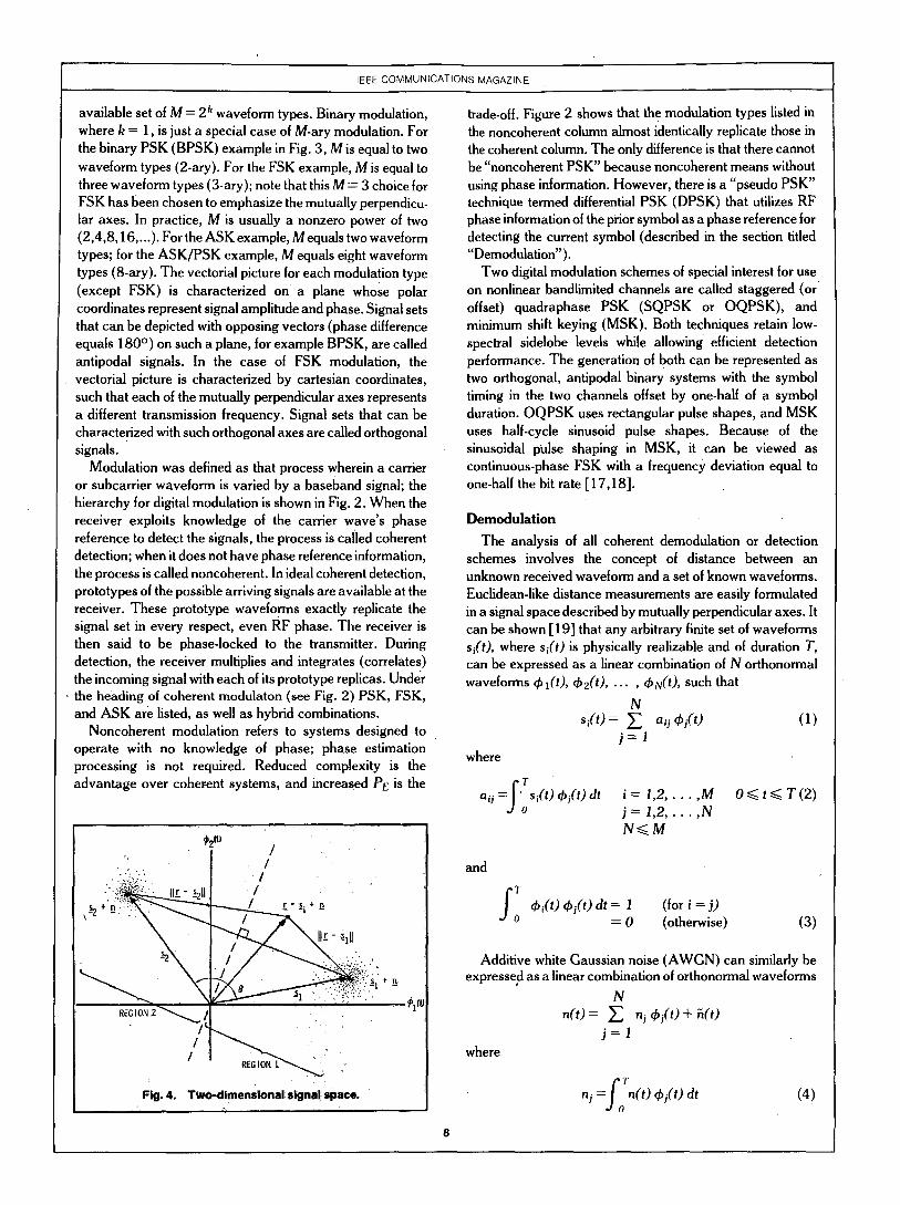
Fig. 4. Two-dimensional signa! space. 1

trade-off. Figure 2 shows that the modulation types listed in the noncoherent column almost identically replicate those in the coherent column. The only difference is that there cannot be “noncoherent PSK” because noncoherent means without using phase information. However, there is a “pseudo PSK’ technique termed differential PSK (DPSK) that utilizes RF phase information of the prior symbol as a phase reference for detecting the current symbol (described in the section titled “Demodulation”).

Two digital modulation schemes of special interest for use on nonlinear bandlimited channels are called staggered (or offset) quadraphase PSK (SQPSK or OQPSK), and minimum shift keying (MSK). Both techniques retain low- spectral sidelobe levels while allowing’ efficient detection performance. The generation of both can be represented as two orthogonal, antipodal binary systems with the symbol timing in the two channels offset by one-half of a symbol duration. OQPSK uses rectangular pulse shapes, and MSK uses half-cycle sinusoid pulse shapes. Because of the sinusoidal pulse shaping in MSK, it can be viewed as continuous-phase FSK with a frequency deviation equal to one-half the bit rate [17,18].

Demodulation The analysis of all coherent demodulation or detection

schemes involves the concept of distance between an unknown received waveform and a set of known waveforms. Euclidean-like distance measurements are easily formulated in a signal space described by mutually perpendicular axes. It can be shown [ 191 that any arbitrary finite set of waveforms si(t), where si ( t ) is physically realizable and of duration T, can be expressed as a linear combination of N orthonormal waveforms +l(t) , +*(t) , ... , +N(t), such that

N

j = l si(t) = aij +j(t) (1)

where

a . . II = J’si(t; +j(t) dt i = 1,2, . . . ,M 0.G t < ~ ( 2 ) 0 j = 1,2, . . . ,N

N G M

and T I c$i(t) +j(t) dt = 1 (for i = j ) 0 = 0 (otherwise) (3)

Additive white Gaussian noise (AWG,N) can similarly be expressed as a linear combination of orthonormal waveforms

n(t) = nj +j(t) + ;(t) N

j = 1 where

nj =JoTn(t) +j(t) dt (4)

8

For the signal detection problem, the noise can be partitioned into two components

n(t) = ;I(t) + ii(t) where

N

j = l is taken to be the noise within the signal space, or the projection of the noise components on the signal axes 4 1 (t) , 42(t), . . . , @N(t), and

Yt) = nj 4i(t) (5)

ii(t) = n(t) - ii(t)

is defined as the noise outside the signal space. In other words, h(t) may be thought of as the noise that is effectively tuned out by the detector. The symbol i(t) represents the noise that will interfere with the detection process, and it will henceforth be referred to simply as n(t). Once a convenient set of N orthonormal functions has been adopted (note that @(t) is not constrained to any specific form), each of the transmitted signal waveforms si(t) is completely determined by the vector of its coefficients

s i = ( a i l , ai2, . . . , a i N ) i = I, 2, . . . , M

Similarly, the noise n(t) can be expressed by the vector of its coefficients

n = (nl, n2, . . . , nN)

where n is a random vector with zero mean and Gaussian distribution.

Since any arbitrary waveform set, as well as noise, can be represented as a linear combination of orthonormal waveforms (see (1)-(5)), we are justified in using (Euclidean-like) distance in such an orthonormal space, as a decision criterion for the detection of any signal set in the presence of AWGN.

Detection in the Presence of A WCN Figure 4 illustrates a two-dimensional signal space, the

locus of two noise-perturbed prototype binary signals (s I + n ) and ( s2 + n) , and a received signal r. The received signal in vector notation is: r=si +n, where i = 1 or 2. This geometric

or vector view of signals and noise facilitates the discussion of digital signal detection. The vectors s I and 8 2 are fixed, since the waveforms sl(t) and s2(t) are nonrandom. The vector or point n is a random vector; hence, r is also a random vector.

The detector’s task after receiving r is to decide whether signal s l or s2 was actually transmitted. The method is usually to decide upon the signal classification that yields the minimum PE, although other strategies are possible [20]. For the case where M equals two signal classes, with S I and s2 being equally likely and the noise being AWGN, the minimum-error decision rule turns out to be: Whenever the received signal r lands in region 1 , choose signal s 1 ; when it lands in region 2, choose signal s2 (see Fig. 4). An equivalent statement is: Choose the signal class such that the distance d(r ,s i ) = I( r - s i 1 1 is minimal, where 1 1 x 1 1 is called the ‘‘norm” of.vector x and generalizes the concept of length.

Detection of Coherent PSK The receiver structure implied by the above rule is

illustrated in Fig. 5. There is one product integrator (correlator) for each prototype waveform (M in all); the correlators are followed by a decision stage. The received signal is correlated with each prototype waveform known a priori to the receiver. The decision stage chooses the signal belonging to the correlator with the largest output (largest z i ) . For example, let:

s I(t) = sin w t s p(t) = - sin w t

n(t)= a random process with zero mean and Gaussian distribution

Assume s l(t) was transmitted, so that:

r(t) = sl(t) + n(t) and z i = r(t) si(t) i t i = 1,2 I’

9

Fig. 7. Signal space and decision regions for 3-ary coherent FSK detection.

The expected values of the product integrators, as illustrated in Fig. 5, are found as follows:

E { zz(t = T) } = E u t + n(t) sin wt dt

where E is the statistical average. The decision stage must decide which signal was

transmitted by measuring its location within the signal space. The decision rule is to choose the signal with the largest value of zi. Unless the noise is large and of a nature liable to cause an error, the received signal is judged to be s ,(t). Note that in the presence of noise this process is statistical; the optimal detector is one that makes the fewest errors on the average. The only strategy that the detector can employ is to “guess” using some;optimized decision rule.

Figure 6 shows the detection process with the signal space in mind. It represents a coherent four-level (4-ary) PSK or quadraphase shift keying (QPSK) system. In the terms we used earlier for M-ary signaling; k = 2 and M = 22 = 4. Binary source digits are collected two at a time, and for each symbol interval the two sequential digits instruct the modulator as to which of the four waveforms to produce. In general, for coherent M-ary PSK (MPSK) systems, si(t) can be expressed as

si(t)= d m c o s ( w o t - 27ri/M) (for 0 < t < T) i 1,2, ... , M

Here, E is the energy content of s , ( t ) , and w o is an integral multiple of Z.rr/T. We can choose a convenient set of orthogonal axes scaled to fulfill (3) as follows

4,(t) = m c o s wot (6) , . +’(t) = m s i n wot

Now si(t) can be writ& in terms of these orthogonal coordinates, giving:

.. ,

si(t) = ,/i?cos(2mi/M) +, ( t ) + fi s in (2dM) +d t ) (7) The decision rule for the detector (see Fig. 6) is to decide

that s ,(t) was transmitted if the received signal point falls in region 1, that sp(t) was transmitted if the received signal point falls in region 2, and so forth. In other words, the decision rule is to choose the ith waveform with the largest value of correlator output z i (see Fig. 5) .

Detection o f Coherent FSK FSK modulation is characterized by the information being

contained in the frequency of the carrier wave. A typical set of signal waveforms is described by

s i ( t ) = d m c o s w i t (forO<t<T) i=1,2, ..., M = O (otherwise)

where E is the energy content of si(t), and ( w ~ + ~ - ai) is an integral multiple of Z.rr/T. The most useful form for the orthonormal coordinates +l(t), &(t) , . . . , +N(t) is

+j(t) = @cos wjt j = I , 2, . .’. , N and, from (2)

a, . ,, = jI COS wit J2/Tcos wjt dt.

Therefore

aij = fl (for .i = j ) = O (otherwise)

In other words, the ith signal point is located on the ith coordinate axis at a displacement *from the origin of the signal space. Figure 7 illustrates the signal vectors (points) and the decision regions for a 3-ary coherent FSK modulation ( M = 3). In this scheme, the distance between any two signal points si and si is constant

d(s,sj) = 1 1 si - s j 1 1 = (for i # j )

As in the coherent PSK case, the signal space is partitioned into M distinct regions, each containing one prototype signal point. The optimum decision rule is to decide that the transmitted signal belongs to the class whose index number is the same as the region where the received signal was found. In Fig. 7, a received signal point r is shown in region 2. Using the decision rule, the detector classifies it as signal s2. Since the

‘ I

Fig. 8. Signal space for DPSK detection. . .

10

noise is a random vector, there is a probability greater than zero that the location of r is due to some signal other than s2. For example, if the transmitter sent 82, then r.is the sum of s2 + n,, and the decision to choose s2 is correct; however, if the transmitter actually sent s3, then r must be the sum of s3 i nb (see Fig. 7), and the decision to select $2 is an error.

Detection of DPSK With noncoherent systems, no provision is made to phase-

synchronize the receiver with the transmitter. Therefore, if the transmitted wavefohn is

Si(t) = J r n c o s ( w ( $ + +i) i = 1 , 2 , . . . , M

r(t) = J m c o s (wet + chi + a) + n(t)

where CY is unknown and is assumed to be randomly distributed between zero and 27~.

For coherent detection, product integrators (or their equivalents) are used; for noncoherent detection, this practice is generally inadequate because the output of a product integrator is a function of the unknown angle CY. However, if we assume that CY varies slowly enough to be considered constant over two, period times (ZT), the relative phase difference between two successive waveforms is independent of a, that is,

the received signal can be characterized by

This is the basis for DPSK modulation. The carrier phase of the previous signaling interval is used as a phase reference for demodulation. Its use requires differential encoding of the message sequence at the transmitter since the information is carried by the difference in phase between two successive waveforms. To send the ith message (i = 1 , 2 , . . . , M), the current signal waveform must have its phase advanced by Zrri/M radians over the previous waveform. The detector can then calculate the coordinates of the incoming signal by product-integrating it with the locally generated waveforms m c o s wot and m s i n wgt. In this way it measures the angle between the current and the previously received signal points (see Fig., 8) [ 191.

One way of viewing the difference between coherent PSK and DPSK is that the former compares the received signal with a clean reference; in the latter however, two noisy signals are compared with each other. Thus, we might say there is twice as much noise in DPSK as in PSK. Consequently, DPSK manifests a degradation of approximately 3 dB when compared with PSK; this number decreases rapidly with increasing signal-to-noise ratio. In general, the errors tend to propagate (to adjacent period times) due to the correlation between signaling waveforms. The trade-off for this performance loss is reduced system complexity.

Detection of Noncoherent FSK A noncoherent FSK detector can be implemented with

correlators such as those shown in Fig. 5 However, the hardware must be configured as an energy detector, without

exploiting phase measurements. For this reason, it is implemented with twice as many channel branches as the coherent detector. Figure 9 illustrates the in-phase (1) channels and quadrature (Q) channels used to detect the signal set noncoherently. Another possible implementation uses filters followed by envelope detectors; the detectors are matched to the signal envelopes and not to the signals themselves. The phase of the carrier is of no importance in defining +e envelope; hence, no phase information is used. In the case of binary FSK, the decision as to whether a “1” or a “0” was transmitted is made on the basis of which of the two envelope detectors has the largest amplitude at the moment of measurement. Similarly, for a multifrequency shift keying (M-ary FSK, or MFSK) system, the decision as to which of the M signals was transmitted is made on the basis of which of the M envelope detectors has maximum output.

Probability of Error The calculations for probability of error (PE), which can be

viewed geometrically (see Fig. 4), involve finding the probability that given a particular signal, say s l , the noise vector n will give rise to a received signal falling outside region 1 ; all PE calculations have this goal. For the general M-ary signaling case, the probability of making an incorrect decision is termed the probability of symbol error, or simply (PE). It is often convenient to specify system performance by the probability of bit error (PB), even when decisions are made on the basis of symbols for which k> 1. PE and PB are related as follows: For orthogonal signals [21],

pB/pE = (2 k- ‘)/(2 - 1) .

For nonorthogonal schemes, such as MPSK signaling, one often uses a binary-to-M-ary code such that binary sequences corresponding to adjacent symbols (phase shifts) differ in only one bit position; one such code is the Gray code. When an M-ary symbol error occurs, it is more likely that only one of the k input bits will be in error. For such signals [3],

Ps P,/log,M = PE/k (for PE << I) For convenience, this discussion is restricted to BPSK (k =

1, M = 2) modulation. For the binary case, the symbol error probability equals the bit error probability. Assume that signal s I( t ) has been transmitted and that r(t) = s 1( t ) + n(t).

11

IEEE COMMUNICATIONS MAGAZINE.

Assuming equally likely signals, and recalling that the decision of region 1 versus region 2 depends on the product integrators and the decision stage (see Fig. 5) , we can write

E J binary = PB = Pr 1 r(t)sz(t) dt >

0

l o 7 ( t ) s I(*) dt I r(t) = s I(t) + n(t)

for 0 < t< T. The solution for the PB expression can be shown to be

1 PB = I/Jz;;j 00

exp(-u2/2) du Eb/No(l -cos 6 )

where Eb is the signal energy per bit in joules, N o is the noise density at the receiver in watts per Hz, and 0 is the angle between s I and sz (see Fig. 4). When 8 = T, the signals are termed antipodal, and the PB becomes

t / - w

The same kind of analysis is pursued in finding the PB expressions for the other types of modulation. The parameter Eb/No in (8 ) can be expressed as the ratio of average signal power to average noise power, S / N (or SNR). By arbitrarily 'introducing the baseband signal bandwidth W, we can write the following identities, showing the relationship between & / N o and SNR

TABLE 1 PROBABILITY OF BIT ERROR FOR SELECTED BINARY MODULATION SCHEMES

.Modulation

Coherent PSK

Coherent FSK

~

where - = E b Lergy/Bit

N o Noise Density

- ' S Signal Power

NOR Noise Density X Bit Rate _-=

and Q(x) = - &J-x:xp(."2/2)d"

where S = average modulating signal power T = bit time duration R = 1/T= bit rate N = N O W

The dimensionless ratio Eb/No (required to achieve a specified P a , is uniformly used for characterizing digital communications system performance. Note that optimum digital signal detection implies a correlator (or matched filter) implementation, in which case the signal bandwidth is equal to the noise bandwidth. Often we are faced with a system model for which this is not the case (less than optimum); in practice, we just reflect a factor into the required E b / N o parameter that' accounts for the suboptimal detection performance. Therefore, required Eb/No can be considered a metric that characterizes the performance of one system versus another; the smaller the required &/NO, the more efficient the system modulation and detection process.

The PB expressions for the binary modulation schemes discussed above are listed in Table I and are graphically compared in Fig. 10. At large SNRs, it can be seen that there is approximately a 4-dB difference between the best (coherent PSK) and the worst (noncoherent FSK). In some cases, 4 dB is a small price to pay for the implementation simplicity gained in going from a coherent PSK to a noncoherent FSK; however, for some applications, even a 1-dB saving is worthwhile. There are other considerations besides PB and system complexity; for example, in some cases (such as randomly fading propagation conditions), a noncoherent system is more robust and desirable because there may be difficulty in establishing a coherent reference.

An exception to Table I and Fig. 10 is worth mentioning, in light of today's bandwidth efficient modulation schemes. MSK modulation, which can be regarded as coherent FSK, manifests error-rate performance equal to BPSK when detected with the appropriate receiver [ 181.

Digital Transmission Trade-offs System trade-offs are fundamental to all digital communi-

cations designs. The goals of the designer are: (1) to

12

AUGUST 1983

maximize transmission bit rate R, (2) to minimize probability of bit error PB, (3) to minimize required power, or relatedly, to minimize required bit energy per noise density Eb/No, (4) to minimize required system bandwidth W, ( 5 ) to maximize system utilization, that is, to provide reliable service for a maximum number of users, with minimum delay and maximum resistance to interference, and (6) to minimize system complexity, computational load, and system cost. The designer usually seeks to achieve all these goals. However, goals (1) and (2) are clearly in conflict with goals (3) and (4); they call for simultaneously maximizing R, while minimizing f B , Eb/No, and w. There are several constraints and theoretical limitations that necessitate the trading-off of any one requirement with each of the others. Some of the constraints are: the Nyquist theoretical minimum bandwidth requirement, the Shannon-Hartley capacity theorem, the Shannon limit, government regulations (for example, frequency allocations), technological limitations (for example, state-of-the-art components), and other system requirements (for example, satellite orbits).

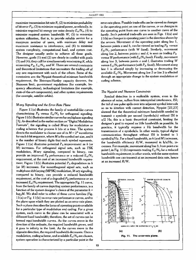
M-ary Signaling and the Error-Rate Plane Figure 1 1 (a) illustrates the family of waterfall-like curves

characterizing f~ versus & , / N o for orthogonal signaling. Figure 11 (b) illustrates similar curves for multiphase signaling [3]. AS described in the earlier section on “Digital Modulation Formats”, the signaling is called Mary for modulation or coding schemes that process k bits at a time. The system directs the modulator to choose one of its M = zk waveforms for each k bit sequence, where Mis the symbol-set size, and k is the number of binary digits that each symbol represents. Figure 1 l(a) illustrates potential PB improvement as k (or M) increases. For orthogonal signal sets, such as FSK modulation, M-ary signaling, compared to binary, can provide an improved Ps performance or a reduced Eb/No requirement, at the cost of an increased bandwidth requirement. Figure 1 l(b) illustrates potential PB degradation as k (or M) increases. For nonorthogonal signal sets, such as multiphase shift keying (MPSK) modulation, M-ary signaling, compared to binary, can provide a reduced bandwidth requirement, a t the cost of a degraded-PB performance or an increased &, /No requirement. The appropriate Fig. 1 1 curve, from the family of curves depicting system performance, is a function of the system designer’s choice of the parameter k = log2M. We shall refer to either of these curve families (Fig. 1 1 (a) or Fig. 1 1 (b)) as error-rate performance curves, and to the plane upon which they are plotted as an error-rate plane. Such a plane describes the locus of operating points available for a particular type of modulation and coding. For a given system, each curve in the plane can be associated with a different fixed bandwidth; therefore, the set,of curves can be termed equi-bandwidth curves. As the curves move in the direction of the ordinate, the required bandwidth grows, until it goes to infinity in the limit. As the curves move in the obposite direction, the required bandwidth decreases. Once a modulation, coding scheme, and available Eb/No are chosen, system operation is characterized by a particular point in the

error-rate plane. Possible trade-offs can be viewed as changes in the operating point on one of the curves, or as changes in the operating point from one curve to another curve of the family. Such potential trade-offs are seen in Figs. 1 l(a) and 1 1(b) as changes in operating point in the direction shown by the arrows. Movement of the operating point along line 1, between points a and b, can be viewed as trading PB versus &/No performance (with w fixed). Similarly, movement along line 2, between points c and d, is seen as trading PB versus Wperformance (with Eb/No fixed). Finally, movement along line 3, between points e and f, illustrates trading W versus E b / N o performance (with PB fixed). Movement along line 1 is effected simply by increasing or decreasing the available Eb/No. Movement along line 2 or line 3 is effected through an appropriate change to the system modulation or

, coding scheme.

The Nyquist and Shannon Constraints Symbol detection in a realizable system, even in the

absence of noise, suffers from intersymbol interference, ISI; the tail of one pulse spills over into adjacent symbol intervals so as to interfere with correct detection: Nyquist [22,23] showed that the theoretical minimum bandwidth needed to transmit x symbols per second (Symbols/s) without IS1 is x / 2 Hz; this is a basic theoretical constraint, limiting the designer’s goal to expend as little bandwidth as possible. In practice, it typically requires x Hz bandwidth for the transmission of x symbols/s. In other words, typical digital communication throughput without IS1 is limited to 1 symbol/s/Hz. For a fixed bandwidth, as k (and M) Increases, ‘

the bandwidth efficiency R/W, measured in b/s/Hz, increases. For example, movement along line 3, from point e to point f, in Fig. 1 1 (b) represents trading & , / N o for a reduced bandwidth requirement; in other words, with the same system bandwidth one can transmit at an increased data rate, hence at an increased R/W.

13

HOGONAL SIGNALING

NORMALIZED ENERGY PER INFORMATION BIT $ I N ~ I ~ B I

(a) (b)

Fig. 11. The error-rate plane.

I

I Fig. 12. Various bandwidth crfterfa. I Shannon [24] showed that the system capacity C , for

channels perturbed by AWCN, is a function of the average received signal power S ; the average noise power N ; and the bandwidth W. The capacity relationship (Shannon-Hartley theorem) can be stated as:

It is possible to transmit information over such a channel at a rate R, where R < C, with an arbitrarily small error rate by using a sufficiently complicated coding scheme. For a rate R > C , it is not possible to find a code which can achieve an arbitrarily small error rate. Shannon's work showed that the values of S, N, and W set a limit on transmission rate, not on accuracy. It can also be shown, from (lo), that the required Eb/No approaches the Shannon limit of -1.6 dB as W increases without bound. At the Shannon limit, shown in Fig. 1 1 (a), and PB curve is discontinuous, going from a value of PB = 1/2 to P B = 0. It is not possible to reach the Shannon limit, because, as k increases without bound, the bandwidth \ requirement and delay become infinite and the implementation complexity increases without bound. Shannon's work predicted the existence of codes that could improve the PB performance or reduce the Eb/No required from the levels of the uncoded binary modulation schemes up to the limiting curve. For P B = BPSK modulation requires an &/No of 9.6 dB (the optimum uncoded binary case). Shannon's work therefore promised a theoretical performance improvement of 1 1.2 dB over the performance of optimum uncoded binary modulation, through the use of coding techniques. Today, most of that promised improvement (approximately 7 dB) is realizable [25]. Optimum system design can best be described as a search for rational compromises or trade-offs amongst the various constraints and conflicting goals.

Bandwidth of Digital Data The theorems of Nyquist and Shannon, though concise

and fundamental, are based on the assumption of strictly

band-limited channels, which means that no signal power whatever is allowed outside the defined band. We are faced with the dilemma that strictly band-limited signals are not realizable since they imply infinite transmission-time delay; non-band-limited signals, having energy at arbitrarily high frequencies, appear just as unreasonable [26]. It is no wonder that there is no single universal, definition of bandwidth.

All criteria of bandwidth have in common the attempt to specify a measure of the width W of a non-negative real- valued spectral density defined for all frequencies I f 1 < m.

Figure 12 illustrates some of the most common definitions of bandwidth; in general, the various criteria are not inter- changable [27]. The power spectral density S(f) for a single pulse takes the analytical form

. ~~

IEEE COMMUNICATIONS MAGAZlNE

14

where f, is the carrier frequency and Tis the symbol duration. This same spectral density, whose general appearance is sketched in Fig. 12, characterizes a sequence of random digital data, assuming the averaging time is long, relative to the symbol duration [28]. The spectral density plot consists of a main lobe and smaller symmetrical side lobes. The general shape of the plot is valid for most digital modulation formats; some formats, however, do not have well defined lobes [28]. The bandwidth criteria depicted in Fig. 12 are:

1) Half-Power Bandwidth: This is the interval between frequencies at which S(f) has dropped to half power, or 3 dB below the peak value.

2) Equivalent Rectangular or Noise Equivalent Band- width: The noise equivalent bandwidth was originally conceived to permit rapid computation of output noise- power from an amplifier with a wide-band noise input; the concept can similarly be applied to a signal bandwidth. The noise equivalent bandwidth of a signal is defined as the value of bandwidth which satisfies the relationship P = WN S(f,), where P is the total signal power over all frequencies, WN is the noise equivalent bandwidth, and S(fJ is the value of S(f) at the band center (assumed to be the maximum value over all frequencies).

3) Null-to-Null Bandwidth: The most popular measure of bandwidth is the width of the main spectral lobe, where most of the signal power is contained. This criterion lacks complete generality since some modulation formats lack well-defined lobes.

4) Fractional Power Containment Bandwidth: This bandwidth criterion has been adopted by the Federal Communications Commission (FCC Rules and Regula- tions Section 2.202) and states that the occupied bandwidth is the band which leaves exactly 0.5% of the signal power above the upper band limit and exactly 0.5% of the signal power below the lower band limit. Thus, 99% of the signal power is inside the occupied band.

5) Bounded Power Spectral Density: A popular method of specifying bandwidth is to state that everywhere outside the specified band S(f) must have fallen at least to a certain stated level below that found at the band center. Typical attenuation levels might be 35 or 50 dB.

The Bandwidth-Efficiency Plane Equation (1 0) can be written as

Eb/No = w/c (2'Iw - I ) . (1 1)

Equation (1 1) has been plotted on the R/W versus Eb/No plane in Fig. 13. We shall term this plane the bandwidth- efficiency plane. The ordinate R/W is a measure of how much data can'be transmitted in a specified bandwidth within a given time; it therefore reflects how efficiently the bandwidth resource is utilized. The abscissa is &/No in decibels. For C = R in (1 l ) , the plotted curve in the plane represents a boundary that separates parameter combinations supporting potential error-free communication from regions where such communication is not possible. Upon the bandwidth-efficiency plane of Fig. 13 are plotted the operating points for MPSK and MFSK modulation, each at PB = Notice that for MPSK modulation, R/W increases with increasing M; however, for MFSK modulation, R/W. decreases with increasing M. Notice also that the location of the MPSK points indicate that BPSK (M = 2) and QPSK (M = 4) require the same Eb/No. That is, for the same value of &, /NO, QPSK has a bandwidth efficiency of 2 b/s/Hz, compared to 1 b/s/Hz for BPSK. This unique feature stems from the fact that QPSK is effectively a composite of two BPSK

REGION FOR

16 -CAPACITY. BOUNDARY

1, ip;; ~6 0 MPSK pB =

m MFSK (noncoherent) pB= lo-> LIMITED

t REGION I Fig. 13. The bandwidth-ettlciency plane.

signals, transmitted on waveforms orthogonal to one another and having the same spectral occupancy. This same feature is illustrated in Fig. 1 I(b), where it can be seen that QPSK (k = 2) signaling has the same PB (not the same symbol error rate) as does BPSK ( k = 1) signaling. Each of the two orthogonal BPSK signals comprising QPSK yields half the bit rate and half the signal power of the QPsK signal; hence the required &/No for a given PB is identical for BPSK and QPSK. Also plotted on the bandwidth-efficiency plane of Fig. 13 are the operating points for noncoherent MFSK modulation at a BER of Notice that the position of the MFSK points indicates that binary FSK, BFSK ( M = 2) and quarternary FSK (QFSK (M = 4)) have the same bandwidth efficiency, even though the former requires greater E b / N o for the same error rate. The bandwidth efficiency varies with the modulation index; if we assume that an equal increment of bandwidth is required for each MFSK tone the system must support, it can be seen that for M = 2, R/W 1 b/s/2 Hz = 1/2; and for M = 4, similarly, R/ W = 2 b/s/4 Hz = 1/2.

The bandwidth-efficiency plane in Fig. 13 is analogous to the error-rate plane shown in Fig. 1 1. The Shannon limit of the Fig. 1 1 plane is.analogous to the capacity boundary of the Fig. 13 plane. The curves in Fig. 1 1 were referred to as equi-bandwidth curves. In Fig. 13, we can analogously describe equi-error-probability curves for various modulation and coding schemes. The curves labeled F B I , PBn, and P B ~ are hypothetical constructions for some arbitrary modulation and coding scheme; the PSI curve represents the largest error probability of the three curves, and the PB3 curve represents the smallest. The general direction in which the curves move for improved PB is indicated on the figure.

Just as potential trade-offs amongst PB, & , / N o , and w were considered for the error-rate plane, so too we can view the same trade-offs on the bandwidth-efficiency plane. Such potential trade-offs are seen in Fig. 13 as changes in operating point in the direction shown by the arrows. Movement of the operating point along line 1 can be viewed as trading Ps versus & , / N o performance, with R/W fixed. Similarly,

' movement along line 2 is seen as trading PB versus W (or R/W) performance, with & , / N o fixed. Finally, movement along line 3 illustrates trading w (or R/W) versus E b / N o performance, with PB fixed. In Fig. 13, as 'in Fig. 11, movement along line 1 is effected simply by increasing or decreasing the available Eb/No. Movement along line 2 or line 3 is effected through appropriate changes to the system modulation or coding scheme.

Power-Limited Systems and Bandwidth-Limited Systems For the case of power-limited systems, in which power is

scarce but system bandwidth is available (for example, a space communication link), the following tradeoffs might be made:

Improved P B performance can.. be achieved by expending bandwidth (for a given Eb/No) .

15

Required Eb/No can be reduced by expending bandwidth (for a given PB).

The error-rate plane of Fig. 1 1 (a) is most useful for examining such potential trade-offs. It is on this plane that we can verify whether or not a candidate code offers improvement in required Eb/No (coding gain) for a specified PB (or whether the code offers improvement in PB for a given E i / N o ) .

Any digital scheme that transmits R = logzM bits in T seconds, using a bandwidth of W Hz, always operates at a bandwidth efficiency of R/W = (logZM)/ WT b/s/Hz. From this expression, it can be seen that signals with small WT products are most bandwidth-efficient. Such signals are generally associated with bandwidth-limited systems in which channel bandwidth is constrained but power is abundant. For this case, the usual objective’ is to design the link SO as to maximize the transmitted data rate over the band-limited channel, at the expense of E b / N o (while maintaining a specified Ps performance level). For band-limited operation, bandwidth efficiency is a useful criterion of system performance, and the bandwidth-efficiency plane of Fig. ‘13 is useful for examining potential trade-offs, such as Eb/No for improved R/W, or degraded PB for improved R/W.

The bandwidth-limited and power-limited regions are shown on the bandwidth-efficiency plane of Fig. 13. Notice that the desirable trade-offs associated with each of these regions are not equitable. For the bandwidth-limited region, large R/W is desired; however as Eb/No is continually

increased, the capacity boundary curve flattens out, and ever-increasing amounts of & , / N o are required to achieve improvement in R/W. A similar law of nature seems to be at work in the power-limited region. Here, a savings in &/No is desired, but the capacity boundary curve is steep; to achieve a small relief in required Eb/No requires a large reduction in R/W (increase in bandwidth for a given data rate).

Digital Communication Tradeoffs

Figure 14 has been configured for pointing out analogies between the two performance planes, the error-rate plane of Fig. 11, and the bandwidth-efficiency plane of Fig. 13. Figures 14(a) and 14(b) represent ‘the same planes as Figs. 1 1 and 13, respectively. They have been redrawn, purposely symmetrical, by choosing appropriate scales. The arrows and their labels, in each case, describe the general effect of moving an operating point in the direction of the arrow by means of appropriate modulation and coding techniques. The notations C, C, and F stand for the trade-off considerations “Gained or achieved,” “Cost or expended,” and “Fixed or unchanged,’’ respectively. The parameters being traded are PB, W, R/W, and P(power or S/N). Just as the movement of an operating point toward the Shannon limit in Fig. 14(a) gains improved P B or lower transmitter power at the cost of bandwidth, so too does movement toward the capacity boundary in Fig. 14(b) gain improved bandwidth efficiency at the cost of increased power or degraded P B .

16

~ ~ ~~

AUGUST 1983

Most often, such trade-offs are examined with a fixed P B (constrained by the system requirement) in mind. Therefore, the most interesting arrows are those having fixed bit-error probability (marked F: PB). There are four such arrows in Fig. ,l4, two on the error-rate plane and two on the bandwidth- efficiency plane. System operation can be characterized by either of these two planes. The planes represent two ways of looking at some of the key system parameters; each plane highlights slightly different aspects of the overall design problem. The error-rate plane tends to find most use with power-limited systems; here, as we move from curve to curve, the bandwidth requirements are only inferred, but the PB is clearly displayed. The bandwidth-efficiency plane is generally more useful for examining bandwidth-limited systems; here, as we move from curve to curve, P B is only inferred, but the bandwidth requirements are explicit, since the ordinate is RIW.

Additional Constraints

We are not as free to make trade-offs as we might like; Government regulations dictate choice of frequencies, bandwidths, transmission power levels, and-in the case o f satellites, orbit selection. The satellite orbit and geometry of coverage fixes the satellite antenna gain. Technological state-of-the-art constrains such items as satellite power transmission and earth station antenna gain. There may be other system requirements (for example, the need to operate under scintillation or interference conditions) that can influence the choice of modulation and coding. The effect of these additional constraints3 to limit the regions of realizable .operation within the error-rate plane and the bandwidth- efficiency plane.

Conclusion In the first part of this paper, we have generated a structure

and hierarchy of key signal processing transformations. We have used this structure as a guide for overviewing the formatting, source coding, and modulation steps. We have also examined potential trade-offs for power-limited systems and bandwidth-limited systems. In Part I1 we will continue to examine the remainder of the signal processing steps outlined in Figs. 1 and 2. Also in Part 11, we will review fundamental link analysis relationships in the context of a satellite repeater channel.

References [l] W.L. Pritchard, “Satellite communication-an overview of the

problems and programs,” Proc. IEEE, vol. 65, pp. 294-307, March 1977.

[2] M.P. Ristenbatt, “Alternatives in digital communications,” Proc. IEEE, June 1973.

[3] W.C. Lindsey, and M.K. Simon, Telecommunication Systems Engineering, Englewood Cliffs, NJ: Prentice-Hall, 1973.

[4] J.J. Spilker, Jr., Digital Communications by Satellite, Englewood Cliffs, NJ: Prentice-Hall, 1977.

[5] V.K. Bhargava, D. Haccoun, R. Matyas, and P.P. Nuspl, Digital Communications bg Satellite, New York, NY: John Wiley and Sons, 1981.

[6] C.B. Feldman’and W.R. Bennett, “Band width and transmission performance,”Bell Syst. Tech. J. , vol. 28, appendix V, pp. 594-595, 1949.

[7] A. Lender, “The duobinary technique for high speed data transmission,” IEEE Trans. Commun. Electron., vol. 82, pp. 214-218, May 1963.

[8] E.R. Kretzmer, “Generalization of a technique for binary data communication,” IEEE Trans. Commun. Tech., pp. 67, 68, Feb. 1966.

[9] S. Pasupathy, “Correlative coding: a bandwidth-efficient signaling scheme,” IEEE Communications Magazine, pp. 4-1 1, July 1977.

[ 101 N.S. Jayant, “Digital coding of speech waveforms: PCM, DPCM, and DM quantizers,” Proc. IEEE, vol. 62, no. 5, pp. 61 1-632, May 1974.

[ 111 B.S. Atal and S.L. Hanover, “Speech analysis and synthesis by linear prediction of the speech wave,” J. Acoust. SOC. Am., vol. 50, pp. 637-655, 1971.

[ 121 J.W. Bayless, S.J. Campanella, and A.J. Coldberg, “Voice signals: bit by bit,” IEEE Spectrum, vol. 10, pp. 28-39, October 1973.

[13] J.L. Flanagan, Speech Analysis, Synthesis, and Perception, 2nd ed., New York, NY: Springer-Verlag, 1972.

[14] R.E. Crochiere and J.L. Flanagan, “Current perspectives in digital speech,” IEEE Communications Magazine, vol. 21, no. 1, pp. 32-40, January 1983.

[15] D. Huffman, “A method for constructing minimum redundancy codes,” Proc. IRE, vol. 40, pp. 1098-1101, May 1952.

[IS] R.C. Callager, Information Theory and Reliable Communication, New York, NY: John Wiley and Sons Inc., 1968.

[17] S.A. Groaemeyer and A.L. McBride, “MSK and offset QPSK modulation,” IEEE Trans. Commun., August 1976.

[18] S. Pasupathy, “Minimum Shift Keying: a spectrally efficient modulation,” IEEE Communications Magazine, pp. 14-22, July 1979.

[ 191 E. Arthurs and H. Dym, “On the optimum detection of digital signals in the presence of white gaussian noise-a geometric interpretation of three basic data transmission systems,” IRE Trans. Commun. Syst., December 1962.

1201 H.L. Van Trees. Detection. Estimation, and Modulation Theory- .--- Part I , New York, NY: John Wiley and Sons, 1968.

1211 A.J. Viterbi, Principlesof Coherent Communications, New York, NY: McCraw-Hill Book Co., 1966.

[22] H. Nyquist, “Certain factors affecting telegraph speed,” Bell Syst. Tech. J . , vol. 3 , pp. 324-326, April 1924.

[23] H. Nyquist, “Certain topics on telegraph transmission theory,” Trans. AIEE, vol. 47, pp. 617-644, April i928.

[24] C.E. Shannon, “A mathematical theory of communication,” Bell Syst. Tech. J. , vol. 27, pp. 379-423 and 623-656, 1948. ’

1251 J.P. Odenwalder, Error Control Coding Handbook, San Diego, CA: Linkabit Corporation, July 15, 1976.

[26] D. Slepian, “On bandwidth,”Proc. IEEE, vol. 64, no. 3, pp. 292-300, March 1976.

[27] R.A. Scholtz, “How do you define bandwidth,” Proc. Int. Telemetering Conf., Los Angeles, CA, vol. 8, pp. 281-288, October 1972.

[28] F. Amoroso, “The bandwidth of digital data signals,” IEEE Communications Magazine, vol. 18, no. 6 , pp. 13-24,November 1980.

Bernard Sklar was born in’New York, NY on September 11, 1927. He received the B.S. degree in mathematics and.science from the University of Michigan, Ann Arbor, MI, in 1949; the M.S.E.E. degree from the Polytechnic Institute of New York, Brooklyn, NY, in 1958; and the Ph.D. degree in engineering from the University of California, Los Apgeles, CA, in 1971.

Dr. Sklar has 30 years of experience with the aerospace/defense industry in a variety of technical design and management positions: from 1953 to 1958 he was a research engineer with Republic Aviation Corp., Farmingdale, NY; from 1958 to 1959 he was a member of the technical staff at Hughes Aircraft Co., Culver City, CA; and from 1959 to 1968 he was a senior staff engineer at Litton Systems, Inc., Canoga Park, CA. In 1968 he joined The Aerospace Corp., El Segundo, CA, where he is currently employed. As Manager of System Analysis, he is involved in the development of satellite communication systems.

He has taught engineering courses during the past 2 5 yyars at the University of California, Los Angeles and lrvine: the University of Southern California, Los Angeles; and West Coast University, Los Angeles. Dr. Sklar is a past chairman of the Los Angeles Council IEEE Education Committee, and has been a Senior Member of the IEEE since 1958. rn

17.

digital comms -tutorial- parte i

Documents