i

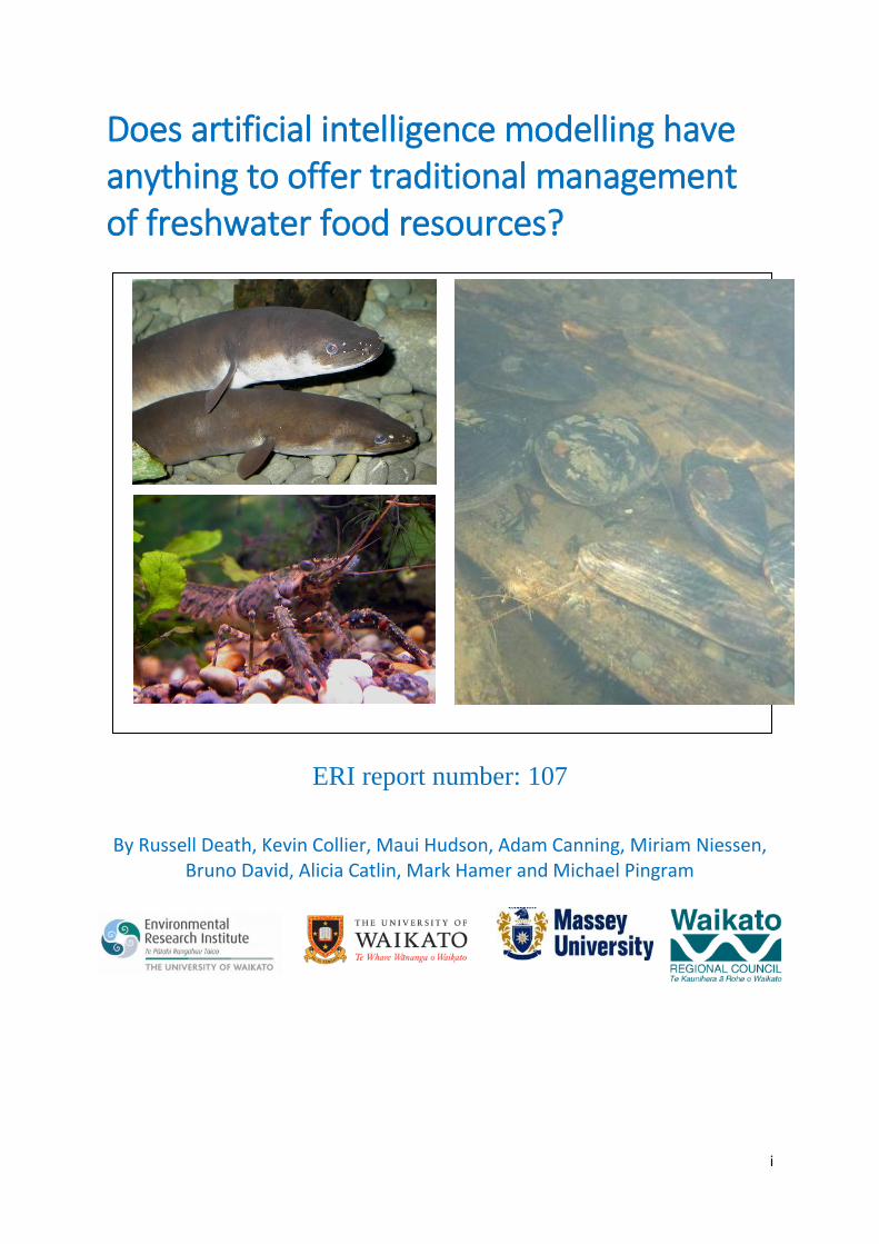
Does artificial intelligence modelling have anything to offer traditional management of freshwater food resources?

ERI report number: 107

By Russell Death, Kevin Collier, Maui Hudson, Adam Canning, Miriam Niessen,

Bruno David, Alicia Catlin, Mark Hamer and Michael Pingram

i

ii

Citation Death RG, Collier KJ, Hudson M, Canning A, Niessen M, David B, Catlin A, Hamer M, Pingram M. 2017. Does artificial intelligence modelling have anything to offer traditional management of freshwater food resources? Environmental Research Institute report no. 107, The University of Waikato, Hamilton Contributing authors Russell Death, Massey University, Palmerston North

Kevin Collier, University of Waikato, Hamilton

Maui Hudson. University of Waikato, Hamilton

Adam Canning, Massey University, Palmerston North

Miriam Niessen, Horizons Regional Council, Palmerston North

Bruno David, Waikato Regional Council, Hamilton

Alicia Catlin, Waikato Regional Council, Hamilton

Mark Hamer, Waikato Regional Council, Hamilton

Michael Pingram, Waikato Regional Council, Hamilton

Cover photo Tuna and kōura (photos by S. Moore); Kākahi (photo K. Collier)

iii

Reviewed by: Approved for release by:

Ian Duggan John Tyrrell Senior Lecturer Research Developer Environmental Research Institute Environmental Research Institute The University of Waikato The University of Waikato

iv

Table of Contents

List of Figures ......................................................................................................................................... iv

List of Tables .......................................................................................................................................... iv

EXECUTIVE SUMMARY ............................................................................................................................ v

ACKNOWLEDGEMENTS ........................................................................................................................... v

Introduction ............................................................................................................................................ 1

Study area ............................................................................................................................................... 3

Methods .................................................................................................................................................. 4

Data sources ....................................................................................................................................... 4

Data analysis ....................................................................................................................................... 6

Results ................................................................................................................................................... 11

Bayesian Belief Networks ................................................................................................................. 11

Boosted Regression Trees ................................................................................................................ 11

Discussion.............................................................................................................................................. 16

Conclusions ........................................................................................................................................... 19

References ............................................................................................................................................ 20

Appendix 1 ............................................................................................................................................ 24

List of Figures

Figure 1: Map of 104 sites sampled for mussels and 256 sites sampled for kōura and eel between

2010 and 2015 in the Waikato region of New Zealand .......................................................................... 5

Figure 2: Bayesian Belief Network for two species of New Zealand freshwater eel .............................. 9

Figure 3: Bayesian Belief Network for two species of New Zealand freshwater mussel ...................... 10

Figure 4: Plot of predicted abundance of A) shortfin eel and B) longfin eel from the BRT model

against the probability of finding the species at that site from the Crow et al. (2014) presence/

absence model. ..................................................................................................................................... 18

List of Tables

Table 1: Results of BRT models for 5 species of mahinga kai in the Waikato Region, including the six

most important variables in predicting the target species and the critical threshold for higher density

or biomass. ............................................................................................................................................ 13

Table 2: Important variables in predicting target mahinga kai species in the Waikato Region grouped

as to whether they are able to be managed of not .............................................................................. 17

v

EXECUTIVE SUMMARY

Management of freshwater systems and the ecosystem services they provide has become a

multi-stakeholder activity. This requires information on resources and how to manage them

to be disseminated to a wide range of users. While artificial intelligence modelling can provide

a powerful tool in managing and understanding resources and their drivers, they can be

confusing to many users. In this study, we explored the potential use of two alternative

modelling approaches (Boosted Regression Trees (BRT) and Bayesian Belief Networks (BBN))

for managing three species of freshwater mahinga kai species–kākahi or kaeo (freshwater

mussel), kōura (freshwater crayfish) and tuna (freshwater eel). While the BBN model is better

for stakeholder communication, the BRT produced more accurate models for all species.

However, variables identified as being important for predicting abundance and biomass of

these species were often environmental parameters that cannot be managed to improve

yield. The artificial intelligence modelling does provide some accurate linkages between the

target species and their environmental drivers. Nevertheless, translating these relationships

into management plans remains challenging. The models are clearly not a panacea for better

resource management, but provide one more tool in the tool box that might assist multi-

stakeholder understanding of how best to manage freshwater resources.

ACKNOWLEDGEMENTS

We thank all those involved in field surveys that have contributed to the data analysed in this

report. The study was funded by the Ministry of Business, Innovation and Employment as part

of the programme Nga Tohu o te Taiao: Sustaining and Enhancing Wai Māori and Mahinga

Kai (contract no. UOWX1304).

Available on a Creative Commons Attribution 3.0 New Zealand Licence

1

Introduction

The management of freshwater resources is becoming an increasingly challenging task as

water abstraction and degradation continue to increase globally (Gleick 1998; Postel and

Richter 2003; Gleick 2014; Richter 2014). This is equally, if not more, challenging for

indigenous peoples faced with the task of managing resources that are often influenced by

factors outside their immediate sphere of control, including climate change. To achieve more

enduring and inclusive outcomes, there is a need to develop ways of using scientific

knowledge alongside traditional knowledge for application in resource management (Berkes

and Berkes 2009; Hudson et al. 2016).

Within science there is a wide range of modelling approaches that are increasingly

being applied to understand ecological systems and to allow for better management of those

systems (Schindler and Hilborn 2015; Houlahan 2017; Stillman Wood and Goss-Custard 2016;

Brudvig 2017). Artificial intelligence (AI) modelling is a subset of those approaches whose

application offers many advantages for dealing with the complexity, level of uncertainty and

large size of data sets that often arise in resource management (Pourret, Naim and Marcot

2008; Crisci, Ghattas and Perera 2012; James et al. 2013; Death 2015; Death et al. 2015;

Kuhn and Johnson 2016). However, even within AI modelling there is an extensive range of

approaches that all have their advantages and disadvantages.

We have previously evaluated the usefulness of a range of modelling approaches in

the New Zealand context, including several AI methods (Collier et al. 2014; Hudson et al.

2016), for informing holistic management of freshwater resources, such as mahinga kai (here

we use mahinga kai to refer to indigenous freshwater species that have traditionally been

used as food, tools, or other resources). In this report, we compare two AI approaches,

Bayesian Belief Networks (BBNs) and Boosted Regression Trees (BRTs), for modelling and

communicating a science perspective for consideration in the management of three

freshwater mahinga kai species–kākahi or kaeo (freshwater mussel), kōura (freshwater

crayfish) and tuna (freshwater eel). Bayesian Belief Networks have been used extensively for

modelling in resource management (Pourret et al. 2008; Death et al. 2015) and are very good

for communicating the interconnectedness of important environmental variables behind the

model working, but are often more challenging for generating accurate models (Uusitalo

2007). In contrast, Boosted Regression Trees (BRTs) seem to be one of the currently preferred

2

modelling tools in ecology (Elith, Leathwick and Hastie 2008) because they can be used to

build models quickly and accurately. However, they are considerably more ‘black box’ in

approach, to the point that the ensemble of multiple regression trees created are not even

visible. The two techniques thus represent a rough contrast from being good for knowledge

transfer but weaker for modelling (BBN), to weaker for communication but more accurate in

predictive capacity (BRT).

Bayesian Belief Networks have been used a number of times to represent traditional

knowledge for resource management (Newton et al. 2006; McGregor et al. 2010). McGregor

et al. (2010) used them for portraying the knowledge on wetland health of traditional owners

in Kakadu National Park, Australia, and Newton et al. (2006) used them to show the impacts

of commercialising non-timber forest products on central-American communities. The

modelling framework of a BBN is initially represented as a conceptual linkage diagram and

this adds to engagement and understanding of the community who can be involved in the

development of the linkage diagram (Liu et al. 2008; Kragt et al. 2011). The BBN is also able

to capture qualitative data more easily than numerically based models; thus outcomes of

‘always’, ‘never’ and ‘sometimes’ are easily translated into a BBN model. Traditional

understanding from experience, informed opinion and non-quantifiable concepts, can also be

incorporated relatively easily into a BBN model. This approach, therefore, offers many

advantages for a range of knowledge forms, including traditional knowledge, although BBNs

are considerably more cumbersome for constructing models, especially as discretisation of

nodes requires creating divisions in usually continuous environmental variables (Death et al.

2015). Boosted Regression Trees have not been used for modelling to support traditional

knowledge as far as we are aware; however, BRTs are now used extensively for ecological and

environmental modelling (Elith et al. 2008).

Most broad-scale modelling of the mahinga kai species examined in New Zealand has

been for predicting presence/absence (Joy 2000; Broad et al. 2001; Joy and Death 2002,

2004; Leathwick et al. 2008a, 2008b, 2010; Crow et al. 2014). Abundance models have been

built, but for a very small number of New Zealand sites: Booker and Graynoth (2013) used

linear regression to model New Zealand eel abundance in 10 rivers, and Jowett, Parkyn and

Richardson (2008) modelled kōura (Paranephrops planifrons) abundance in 30 rivers using

Generalised Additive Models (GAMs). Presence/absence models are likely to be less helpful

for indigenous peoples who might want to use those species as a sustainable food resource.

3

Rather, it will be more important to know whether there is a good size population suitable for

harvesting, rather than knowing that the probability of detecting at least one individual of a

species is high. Although both of these outcomes can be achieved with models, the types of

model that will be useful for either goal may be quite different.

In this report, we compare the efficiency of the two modelling approaches on five

culturally important freshwater species to Māori: two species of freshwater mussel

(Echyridella aucklandica and E. menziesii), one species of freshwater crayfish (P. planifrons)

and two species of freshwater eel (Anguilla dieffenbachii and A. australis). We used data

collected from 100 – 250 rivers in the Waikato region (2.5 million hectares) of the North

Island, New Zealand, to model abundance. Additionally, for eels we also estimated total and

per fish biomass (based on length), as both population parameters are likely to be more

important for management of these species as traditional food resources.

Study area

The Waikato region covers 2.5 million hectares across latitudes 36o and 39oS in New Zealand’s

central North Island, including New Zealand’s largest lake (Taupō) and longest river (Waikato).

Landforms range from active volcanoes (up to 2,797 m a.s.l.) and upland plateau (c. 600 m

a.s.l.) in the south of the region, to steep erodible hill-country (300 – 600 m a.s.l.) along the

west coast, through the central parts of the region and towards the east, and extensive

lowland peatlands and plains in the north. The region is very diverse geologically with

extensive areas of volcanic rock (rhyolites, andesites, basalts and dacites) around the

southern and western volcanoes and eastern peninsula (McCraw 1971), with limestone

common along western parts of the region. Pre-European vegetation cover was

predominantly podocarp-hardwood forest in hill-country and western areas, with extensive

areas of beech in the south. Fernland/scrubland also occurred over wide areas prior to

European colonisation, and sub-alpine grassland and scrubland still occurs at higher altitudes

on the southern mountains.

Average annual rainfall is variable, but lower in the north (1,000 – 1,500 mm p.a.) than

in the eastern and western ranges (up to 2,500 mm p.a.), and high (5,000 mm p.a.) on

southern mountaintops. Mean annual air temperatures in most of this region are in the range

12.5 to 15.0oC, but decline to <8.0oC on southern mountains (Kilpatrick 1999). Most of the

4

Waikato region has been developed for pastoral agriculture or pine forestry, with extensive

remnants of original forest persisting only in upland parts of region (28% of pre-European

extent).

Methods

Data sources

Biological data

Biological data were supplied from Waikato Regional Council environmental monitoring

records. Two mussel species, E. aucklandica and E. menziesii were surveyed by visual/tactile

inspection at 104 sites between 2010 and 2015 in the western Waikato region (Fig. 1). P.

planifrons (kōura) and longfin and shortfin eel were sampled 256 times at 127 locations

throughout the Waikato region between 2010 and 2016 using electro-fishing (Joy, David and

Lake 2013) (Fig. 1). More detail on sampling methodology and fish collected can be found in

(David et al. 2016). Eel length measurements recorded in the field were converted to biomass

using the specific weight length relationships for each species of eel provided in (Jellyman et

al. 2013).

Environmental field data

Concomitant with biological sampling, standard Regional Ecological Monitoring of Streams

(REMS) field methods were used for qualitative assessment or measurement of sampling

reach canopy cover/shade, fencing, dissolved oxygen, temperature, conductivity, wetted

width, thalweg depth (maximum depth at transects), percent macrophyte cover, percent

substrate size (clay, silt, sand, small gravel, etc), and percent wood (Collier and Kelly 2005).

Water samples were collected at some sites for ammonia/ metal/ hardness analysis.

5

Figure 1: Map of 104 sites sampled for mussels (blue circles) and 256 sites sampled for kōura and eel (orange circles) between 2010 and 2015 in the Waikato region of New Zealand

0 10 20 30 405Kilometers

Text

.

6

GIS data

GIS environmental data on nutrients, flow regime, catchment geology and topography,

temperature and shading, MCI (Macroinvertebrate Community Index) and deposited

sediment for each sampled reach were included in the model construction as potential

predictor variables in BRT models. Modelled nutrient, MCI and E. coli were sourced from

Unwin and Larned (2013), flow data from Booker and Woods (2014), catchment geology,

topography and temperature from the Freshwater Ecosystems of New Zealand (FENZ)

database (Leathwick et al. 2010), and modelled sediment data from Clapcott, Goodwin and

Snelder (2103). Subsets of these data considered relevant to specific species were used for

constructing BBNs (see below). Consideration of both commercial (in the case of eels),

traditional and recreational harvest from sampling locations was not possible as, to the best

of our knowledge, there are no site-specific records of commercial, recreational or cultural

collections of the focal species.

Data analysis

Bayesian Belief Networks

BBNs were constructed for mussels and eels using NeticaTM 5.02 software (Pourret, Naim and

Marcot 2008). The network linkage diagram was developed slightly differently for each of the

target species, reflecting the individualised approach to target variables and model

architecture that is possible with BBNs. For the two species of freshwater tuna (Fig. 2), nodes

and the discretisation of those nodes were developed from a review of all the relevant

literature on New Zealand freshwater eels (Niessen et al. in prep). The BBN was then

populated with data from the 127 electro-fished sites. Conditional Probability Tables (CPTs)

were developed with the expectation-maximisation algorithm (EM Learning) in NeticaTM from

the compiled data. The expectation–maximisation (EM) algorithm is an iterative method for

finding maximum likelihood estimates of parameters in statistical models, where the model

depends on unobserved latent variables (Do and Batzoglou 2008). CPTs calculate the

probability of each state in a node occurring, given each combination of conditions in the

parent (input) nodes.

The kākahi BBN was developed for the combined abundance of both species as they

were not expected to be differentiated during traditional food collections. Biota and/or

environment matching analyses using the BVSTEP method on a Euclidean distance

7

resemblance matrix were conducted in Primer 7 (Primer-E Ltd, Plymouth, U.K.; version 7.0.7)

using density per m2 of stream bed and density per m of stream channel as many mussels

were collected associated with banks. The BVSTEP algorithm successively adds and removes

a variable to get the optimum correlation between the environmental and biological data.

Recurrent and dominant variables identified by these analyses were grouped into

intermediate nodes representing access for fish which are an important host for larval kākahi,

physicochemical conditions, riparian conditions and instream habitat conditions. These

intermediate nodes were subsequently linked to kākahi abundance. Variables were

discretised into thirds for all nodes based on their data distributions or professional

judgement. Conditional Probability Tables (CPTs) for the data from 104 sites were again

developed using the expectation-maximisation algorithm (EM Learning) in NeticaTM.

Models were evaluated by hold-out validation with a randomly selected 10% subset

of the training data. There are a wide range of metrics that can be used to evaluate model fit

and performance (for a detailed review see Witten, Frank and Hall (2011); Marcot (2012)).

We used several commonly used metrics that assess both raw predictive ability and ability

relative to occurrence. The percentage of incorrect predictions (percent error) is a simple,

easily understood metric but is sensitive to the number and size of the nodes. For example, if

you have a very common state in the node and predict it will always occur (P=1.0) then you

have a high probability of being correct simply because it usually occurs. For BBNs, Spherical

payoff is similar to the area under receiver operating curves (Hand 1997; Marcot 2012).

Cohen’s kappa also ranges from 0 to 1, with 1 being perfect classification that also assesses

correct predictions relative to how common a state actually is (Boyce et al. 2002; Olden,

Lawler and Poff 2008). The logarithmic loss score (Dlamini 2010) was used to compare BBNs

of alternate architecture. The index ranges from 0 to infinity, with 0 the best possible score.

Unlike the indices above that must be calculated outside NeticaTM, this index is provided

within the program and gives a quick metric for evaluating alternate BBNs.

Boosted Regression Trees

Boosted regression trees (BRTs) are a powerful modification of classification and regression

tree analyses that are now widely used in ecological research (De'ath and Fabricius 2000; Elith

et al. 2008). BRTs combine the algorithms of regression trees, that relate predictors of a single

response variable by recursive binary splits, and boosting, an ensemble method that

8

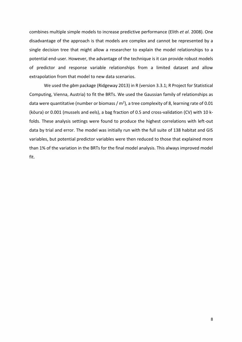
combines multiple simple models to increase predictive performance (Elith et al. 2008). One

disadvantage of the approach is that models are complex and cannot be represented by a

single decision tree that might allow a researcher to explain the model relationships to a

potential end-user. However, the advantage of the technique is it can provide robust models

of predictor and response variable relationships from a limited dataset and allow

extrapolation from that model to new data scenarios.

We used the gbm package (Ridgeway 2013) in R (version 3.3.1; R Project for Statistical

Computing, Vienna, Austria) to fit the BRTs. We used the Gaussian family of relationships as

data were quantitative (number or biomass / m2), a tree complexity of 8, learning rate of 0.01

(kōura) or 0.001 (mussels and eels), a bag fraction of 0.5 and cross-validation (CV) with 10 k-

folds. These analysis settings were found to produce the highest correlations with left-out

data by trial and error. The model was initially run with the full suite of 138 habitat and GIS

variables, but potential predictor variables were then reduced to those that explained more

than 1% of the variation in the BRTs for the final model analysis. This always improved model

fit.

9

Figure 2: Bayesian Belief Network for two species of New Zealand freshwater eel

10

Figure 3: Bayesian Belief Network for two species of New Zealand freshwater mussel

11

Results

Bayesian Belief Networks

The ability of the tuna BBN (Fig. 2) to describe abundance of both species of eel in the training

data was moderate. There was a 36.6% error rate, a logarithmic loss score of 0.42 (this ranges

from 0 to infinity, with 0 the best possible score), a spherical payoff score of 0.78 (this ranges

from 0 to 1, with 1 being the best possible score) and a Cohen’s kappa of 0.65 (indicative of

good model fit) (Landis and Koch 1977). However, the BBN did not perform well on 10% of

the data left out of the model building (independent data); there was a 54.2% error rate, a

log loss score of 2.45, a spherical payoff score of 0.34 and a Cohen’s kappa of 0.21.

The architecture for the kākahi BBN is presented in Figure 3. The ability of the network

to describe the training data was good. There was a 10.6% error rate, a logarithmic loss score

of 0.22 (this ranges from 0 to infinity, with 0 the best possible score), a spherical payoff score

of 0.92 (this ranges from 0 to 1, with 1 being the best possible score) and a Cohen’s kappa of

0.80 (indicative of good model fit). However, the BBN did not perform well on independent

data; there was a 46.2% error rate, a log loss score of 1.75, a spherical payoff score of 0.63

and a Cohen’s kappa of 0.12.

Boosted Regression Trees

The BRT for kōura density had a CV correlation coefficient of 0.778 ± 0.066, with conductivity,

stream width, substrate diversity, segment flow, flood size and distance to the coast

explaining the highest percentage of density variation (Table 1). Kōura are more abundant in

small streams (<1 m wide) within 200 km of the coast, that have high substrate diversity, low

conductivity (<5 mS/m) and small floods (Table 1, Appendix 1).

E. menziesii were generally more abundant than E. aucklandica so the BRT for total

mussel density was dominated by the former species. It had a CV correlation coefficient of

0.528 ± 0.063. E. aucklandica and E. menziesii had CV correlation coefficients of 0.431 ± 0.068

and 0.540 ± 0.068, respectively. Flood size, catchment area and deposited sediment were

dominant predictor variables for both species of kākahi, whereas the presence of

Gobiomorphus huttoni (redfin bully) and large wood were important for E. menziesii only,

with water temperature, slope and stream width important for E. aucklandica only (Table 1,

Appendix 1).

12

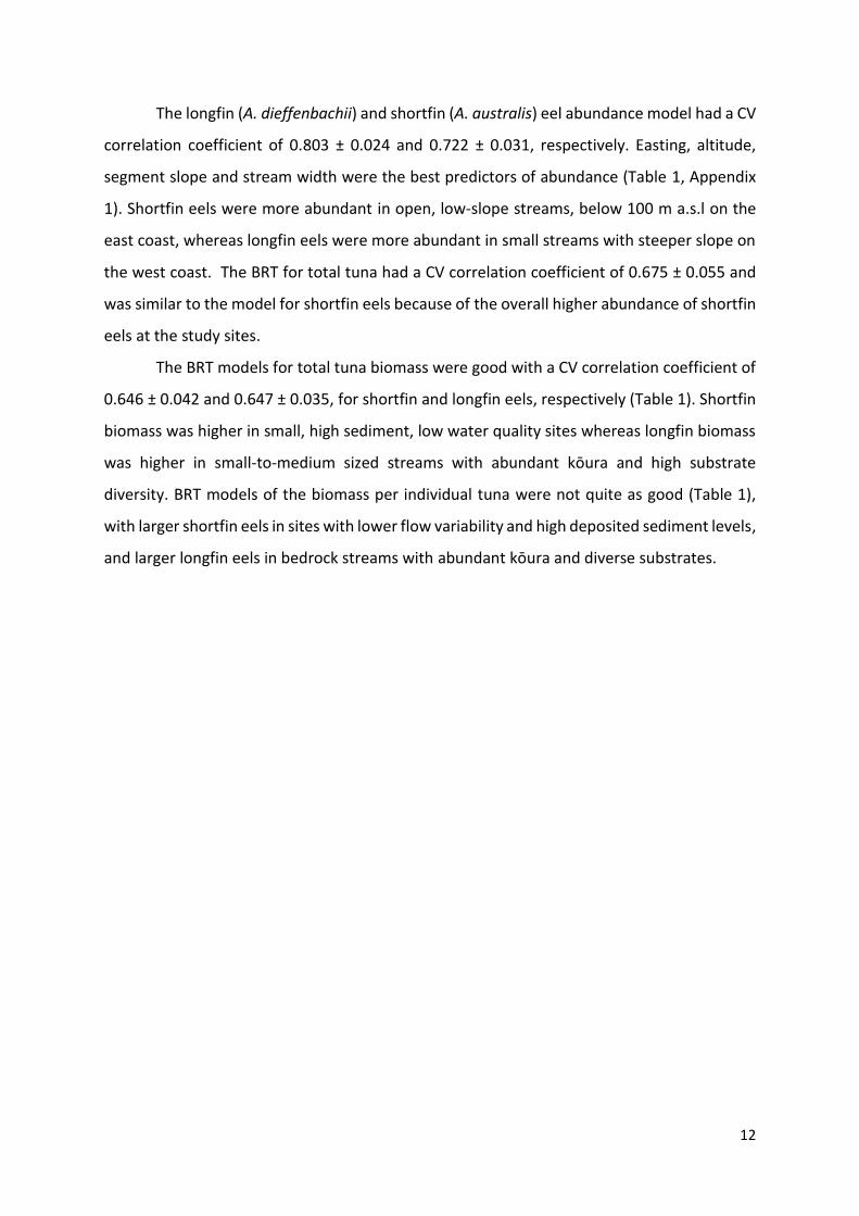
The longfin (A. dieffenbachii) and shortfin (A. australis) eel abundance model had a CV

correlation coefficient of 0.803 ± 0.024 and 0.722 ± 0.031, respectively. Easting, altitude,

segment slope and stream width were the best predictors of abundance (Table 1, Appendix

1). Shortfin eels were more abundant in open, low-slope streams, below 100 m a.s.l on the

east coast, whereas longfin eels were more abundant in small streams with steeper slope on

the west coast. The BRT for total tuna had a CV correlation coefficient of 0.675 ± 0.055 and

was similar to the model for shortfin eels because of the overall higher abundance of shortfin

eels at the study sites.

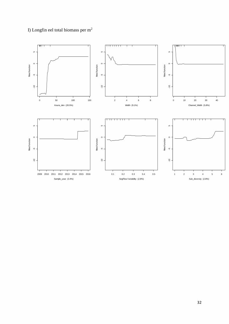
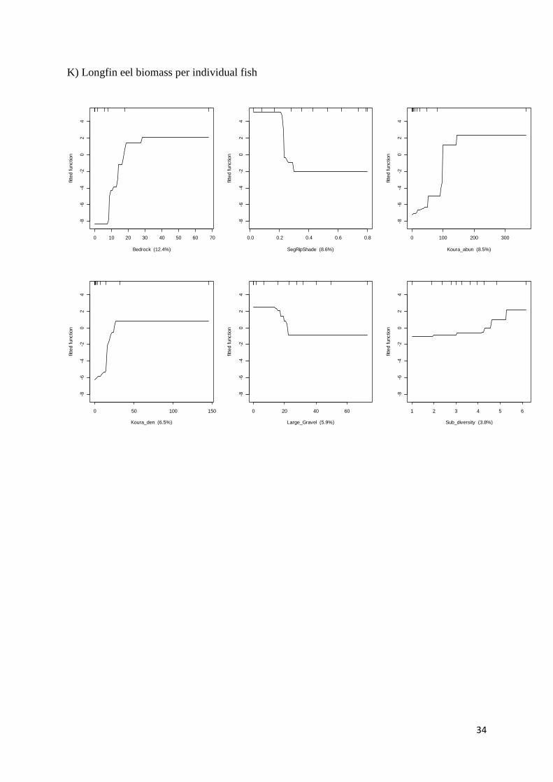
The BRT models for total tuna biomass were good with a CV correlation coefficient of

0.646 ± 0.042 and 0.647 ± 0.035, for shortfin and longfin eels, respectively (Table 1). Shortfin

biomass was higher in small, high sediment, low water quality sites whereas longfin biomass

was higher in small-to-medium sized streams with abundant kōura and high substrate

diversity. BRT models of the biomass per individual tuna were not quite as good (Table 1),

with larger shortfin eels in sites with lower flow variability and high deposited sediment levels,

and larger longfin eels in bedrock streams with abundant kōura and diverse substrates.

13

Table 1: Results of BRT models for 5 mahinga kai species in the Waikato Region, including the six most important variables in predicting the target species (first row), the percent variation explained (second row) and the critical threshold for higher density or biomass (third line) (more detail for the latter is in Appendix 1). Note: FRE3 = flow 3 times median flow; Pr = probability

Training data correl.

Cross-validated data correl.

Standard error for CV correl.

Variables that explain the most variation in the data, the percentage they explain and critical threshold of greater x (where x is the number in the third row)

Kōura relative abundance

0.997 0.778 0.066 Conductivity (mS/m)

Width (m)

Substrate diversity

Segment flow (m3/sec)

Mean annual flood size (m3/sec)

Distance to coast (km)

16.76 10.64 5.97 5.65 5.17 4.42 < 5 < 1 > 5 < 0.05 < 3 < 200

Echyridella aucklandica

0.631 0.431 0.068 Temperature (°C)

Downstream maximum slope (°)

Mean annual flood size(m3/sec)

Catchment area (km2)

Modelled sediment (g/m2)

Width at MALF (Mean Annual Low Flow (m)

21.69 17.72 15.89 8.52 8.52 6.36 < 14 < 3 > 20 > 5000000 < 1 > 5

Echyridella menziesii

0.787 0.54 0.068 Redfin bully (Pr)

Mean annual flood size (m3/sec)

Large wood

Catchment area (km2)

Deposited sediment (g/m2)

Upstream calcium (g/m3)

11.89 11.42 9.82 8.33 7.7 7.58 > 0.65 > 10 > 5 > 5000000 > 15 > 2

Total mussel 0.768 0.528 0.063 Redfin bully (Pr)

Mean annual flood size (m3/sec)

Temperature (°C)

Catchment area (km2)

Large wood (%)

Width at MALF (m)

14.68 13.34 10.01 9.1 8.15 6.29 > 0.65 > 10 < 14 > 5000000 > 5 > 5

Shortfin eel relative abundance

0.953 0.722 0.031 Downstream maximum slope (°)

Altitude (m a.s.l.)

Segment riparian shade (Proportion)

Upstream calcium (g/m3)

Easting (NZMG)

Substrate diversity

11.08 6.83 5.01 4.69 4.53 4.51

14

< 4 < 100 < 0.2 > 2 > 1820000 < 2

Longfin relative abundance

0.959 0.803 0.024 Easting (NZMG)

Gradient (°) Segment slope (°)

Width (m) FRE3 (m3/sec)

Catchment area (km2)

30.67 10.06 7.4 6.49 3.74 3.7 < 175000 > 3 > 2.5 < 1 > 18 < 1000000

Total eel relative abundance

0.963 0.675 0.055 Altitude (m a.s.l)

Easting (NZMG)

Downstream maximum slope (°)

Segment CLUES nitrogen (ppb)

Large gravel (%)

Width (m)

8.27 5.78 5.12 5.04 4.68 4.38 < 100 1750000 < x <

1820000 < 2 > 2 > 50% < 1

Shortfin eel total biomass

0.891 0.646 0.042 MCI Dissolved ogygen (%)

Segment Clues nitrogen (ppb)

Depth (m) Modelled sediment (g/m2)

Nitrate nitrogen (mg/l)

11.22 6.25 5.66 5.58 5.51 3.74 < 85 < 82% > 3 < 0.12 > 80 > 1.25

Longfin eel total biomass

0.964 0.647 0.035 Kōura density

Width (m) Channel width (m)

Sample year

Segment flow variability

Substrate diversity

20.47 9.09 5.78 3.44 2.81 2.81 > 50 < 2 < 2 > 2013 > 0.24 > 5.5

Shortfin eel biomass / individual

0.692 0.608 0.067 Segment flow variability

Mean annual flood size (m3/sec)

Modelled sediment (g/m2)

Emergent exotic macrophytes (%)

Total phosphorous (mg/L)

Segment flow variability

16.84 15.08 12.28 6.52 5.59 5.48 < 0.02 < 1 > 90 > 50 > 0.055 < 0.1

15

Longfin eel biomass / individual

0.72 0.469 0.06 Bedrock (%) Segment riparian shade (proportion)

Kōura abundance

Kōura density

Large gravel (%)

Substrate diversity

12.41 8.61 8.51 6.53 5.93 3.84 > 30 < 0.2 > 120 > 30 < 20 > 5.5

16

Discussion

The Boosted Regression Trees (BRT) performed better at modelling the focal species than the

Bayesian Belief Networks (BBN) despite the BBNs being developed with variables selected a

priori as potentially the most important for determining the abundance of the target species.

The advantage of the BRTs is that they can select from the full suite of potential predictor

variables in the specific dataset, rather than from a smaller, discretised list of potentially

important variables. The logistical requirements of BBN construction essentially limit their

ability to flexibly model the data. Furthermore, discretisation is difficult with many biological

variables as they are continuous (Death et al. 2015).

As highlighted in the introduction, the BBNs are extremely useful for communicating

the casual pathways of environmental influences on species populations, but if the actual

predictive ability of the models is low then their educational merit is moot. It would be better

to construct a diagram of the casual pathways once the important environmental drivers have

been determined with a BRT. However, if mutual participation in the modelling is critical for

buy-in, this approach may not provide a useful modelling tool for incorporating traditional

knowledge.

Previous predictive spatial models of fish and invertebrate species for New Zealand

rivers have focused on predicting presence/absence of those species at a specific site (Joy and

Death 2002, 2004; Leathwick et al. 2005, 2008a, 2008b; Crow et al. 2014). However, for

management of a food resource it is likely to be more important to identify sites where

abundance is above a certain threshold rather than whether there is a high probability of

finding a particular species. There are no current models for kākahi or kōura, but there are

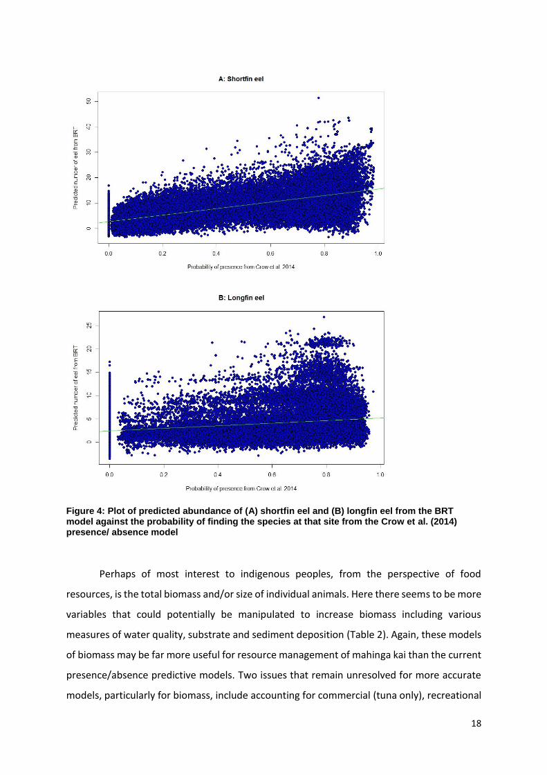
for both species of tuna. There is a weak relationship (F1,48278 = 41478, P < 0.001, r2=0.46 and

F1,48278 = 3133, P < 0.001, r2=0.06) between the predicted abundance of the two species of

tuna from the BRT model and the probability of finding the species at a site from the Crow et

al. (2014) presence/absence model (Fig. 4). Thus, a high probability of finding tuna does not

necessarily translate into there being a high abundance of tuna at a site. It would therefore

seem far more sensible to focus on modelling abundance of a species rather than

presence/absence for managing traditional food resources.

17

Table 2: Important variables in predicting target mahinga kai species in the Waikato Region grouped as to whether they are able to be managed of not. A “?” designates it may be challenging to manage

Kōura numbers Kākahi numbers Tuna numbers Tuna biomass

Can be managed Substrate diversity Deposited sediment Segment riparian

shade

Segment riparian

shade

? Conductivity Large wood Substrate diversity ? DO percent

Temperature

Large gravel

? Redfin bullies

Substrate diversity

? Width MALF

Nitrate

Total Phosphorous

Deposited sediment

? MCI

Beyond influence Distance to coast Catchment area Altitude Bedrock

Mean annual flood

size

Downstream

maximum slope

Downstream

maximum slope

Channel width

Segment flow Mean annual flood

size

Easting Depth

Width Upstream calcium FRE3

Gradient Emergent exotic

macrophytes

Segment slope Kōura density

Upstream Calcium Mean annual flood

size

Catchment area Sample year

Width Segment flow

variability

Segment low flow

Width

18

Figure 4: Plot of predicted abundance of (A) shortfin eel and (B) longfin eel from the BRT model against the probability of finding the species at that site from the Crow et al. (2014) presence/ absence model

Perhaps of most interest to indigenous peoples, from the perspective of food

resources, is the total biomass and/or size of individual animals. Here there seems to be more

variables that could potentially be manipulated to increase biomass including various

measures of water quality, substrate and sediment deposition (Table 2). Again, these models

of biomass may be far more useful for resource management of mahinga kai than the current

presence/absence predictive models. Two issues that remain unresolved for more accurate

models, particularly for biomass, include accounting for commercial (tuna only), recreational

19

and/or customary harvest pressure, for which there are no data. Clearly, managing a resource

without any records or estimates of harvest is extremely difficult. In small streams commercial

harvest pressure may be low, but the impact, even if only decadal, may be quite severe for

population biomass recovery. We also used electrofishing data collected by the local

environment agency rather than the more traditional harvest technique of netting.

Electrofishing is not as effective in deep water where larger eels are found in wadeable

streams during the day. It is more effective in shallower streams where there tend to be fewer

large eels because of the shallower conditions. However, netting is a passive technique suited

to deeper water that catches proportionally larger eels from a larger spatial area.

Furthermore, nets for traditional harvest may also be baited drawing from an even larger

area. Finally, there are no models that assess the condition of the target species. Many

tangata whenua (local people) have commented to us that while tuna may still be present,

many are often now not suitable for consumption because of high parasite loads (R Death,

pers comm.).

The utility of both modelling approaches to assist indigenous aspirations for directly

managing traditional food resources may be limited because most of the important

environmental drivers of species abundance are characteristics of environmental drivers

beyond the ability of iwi to manage (e.g. location, altitude, flood regimes, catchment area and

stream slope; Table 2). For example, kōura BRT models were strongly influenced by

conductivity and substrate diversity, while kākahi models were influenced by the abundance

of redfin bully, which prefer good water quality and unimpeded sea access, the presence of

large wood and deposited sediment levels. There are some notable exceptions where local

scale drivers were identified, however (Table 2), but only riparian shade and substrate

diversity could be manipulated to affect tuna density; ironically, increasing density

(predominantly for shortfin eels) is linked with declines in both these measures.

Conclusions

It can often be challenging for government agencies to develop resource management plans

related to traditional food gathering sites and species as the knowledge of those sites may

have been lost or be difficult to collect. Predictive abundance models of key species may offer

potential for government agencies to take account of indigenous people’s aspirations at sites

20

with high resource value even when that knowledge is lost or unavailable. They can also

provide a mechanism for discussing the opportunities for environmental management actions

to affect those populations, especially if all parties have been involved in the collection of

data and model development, and construction of model architecture.

So are artificial intelligence models useful for traditional management of freshwater

food resources? They can certainly provide objective and accurate models for linking target

species with key environmental drivers from a large range of potential variables. However,

these drivers may not necessarily be those that can be managed and/or those that have

previously been held to be important, particularly when the scale of the model may differ

from that of traditional management actions. They will, however, provide a useful starting

point for conversations and/or management strategies for these species. While artificial

intelligence models may seem to be a very powerful and useful tool, if people are not

comfortable with their use or their predictions then they will no longer be useful. We found

that developing that comfort can be challenging and to take quite some time. We also found

that visual presentation of the findings at locations where participants can verify the

outcomes based on their own knowledge greatly helps with their acceptance of the results.

References

Berkes F. and Berkes M. (2009) Ecological complexity, fuzzy logic, and holism in indigenous knowledge. Futures, 41, 6-12.

Booker D.J. and Graynoth E. (2013) Relative influence of local and landscape-scale features on the density and habitat preferences of longfin and shortfin eels. New Zealand Journal of Marine and Freshwater Research, 47, 1-20.

Booker D.J. and Woods R.A. (2014) Comparing and combining physically-based and empirically-based approaches for estimating the hydrology of ungauged catchments. Journal of Hydrology, 508, 227-239.

Boyce M.S., Vernier P.R., Nielsen S.E. and Schmiegelow F.K.A. (2002) Evaluating resource selection functions. Ecological Modelling, 157, 281-300.

Broad T.L., Townsend C.R., Arbuckle C.J. and Jellyman D.J. (2001) A model to predict the presence of longfin eels in some New Zealand streams, with particular reference to riparian vegetation and elevation. Journal of Fish Biology, 58, 1098-1112.

Brudvig L.A. (2017) Toward prediction in the restoration of biodiversity. Journal of Applied Ecology, 54, 1013-1017.

Clapcott J., Goodwin E. and Snelder T.H. (2103) Predictive Modesl of Benthic Macroinvertebrate Metrics. Vol. REPORT NO. 2301. Cawthron Institute, Nelson.

Collier K. and Kelly J. (2005) Regional Guidelines for Ecological Assessments of Freshwater Environments. Macroinvertebrate Sampling in Wadeable Streams. Environment Waikato Technical Report TR2005/02. Environment Waikato, Hamliton. (http://www.ew.govt.nz/publications/technicalreports/tr0502.htm),

21

Collier K.J., Death R.G., Hamilton D.P. and Quinn J.M. (2014) Potential Science Tools to Support Mahinga Kai Decision Making in the National Objectives Framework. Environmental Research Institute, The University of Waikato, Hamilton.

Crisci C., Ghattas B. and Perera G. (2012) A review of supervised machine learning algorithms and their applications to ecological data. Ecological Modelling, 240, 113-122.

Crow S., Booker D., Sykes J., Unwin M. and Shankar U. (2014) Predicting distributions of New Zealand freshwater fishes. Vol. Client Report CHC2014-145. NIWA, Christchurch.

David B., Bourke B., Hamer M., Scothern S., Pingram M. and Michael L. (2016) Incorporating fish monitoring into the Waikato Regional Councils’ Regional Ecological Monitoring of Streams (REMS) – preliminary results for wadeable streams 2009-2015., Vol. Waikato Regional Council Technical Report 2016/29. Waikato Regional Council.

De'ath G. and Fabricius K.E. (2000) Classification and regression trees: A powerful yet simple technique for ecological data analysis. Ecology, 81, 3178-3192.

Death R.G. (2015) An environmental crisis: science has failed let’s send in the machines. WIREs Water. Death R.G., Death F., Stubbington R., Joy M.K. and Van Den Belt M. (2015) How good are Bayesian

belief networks for environmental management? A test with data from an agricultural river catchment. Freshwater Biology, 60, 2297-2309.

Dlamini W.M. (2010) A Bayesian belief network analysis of factors influencing wildfire occurrence in Swaziland. Environmental Modelling and Software, 25, 199-208.

Do C.B. and Batzoglou S. (2008) What is the expectation maximization algorithm? Nat Biotech, 26, 897-899.

Elith J., Leathwick J.R. and Hastie T. (2008) A working guide to boosted regression trees. Journal of Animal Ecology, 77, 802-813.

Gleick P.H. (1998) Water in crisis: paths to sustainable water use. Ecological Applications, 8, 571-579. Gleick P.H. (2014) The world's water. Volume 8 : the biennial report on freshwater resources. p. 1

online resource (420 pages). Hand D.J. (1997) Construction and assessment of classification rules, Wiley, Chichester ; New York. Houlahan J.E. (2017) The priority of prediction in ecological understanding. Oikos, 126, 1-7 Hudson M., Collier K., Awatere S., Harmsworth G., Henry J., Quinn J., Death R., Hamilton D., Te Maru

J., Watene-Rawiri E. and Robb M. (2016) Integrating Indigenous Knowledge into Freshwater Management. The International Journal of Science in Society, 8.

James G., Witten D., Hastie T. and Tibshirani R. (2013) An introduction to statistical learning : with applications in R.

Jellyman P.G., Booker D.J., Crow S.K., Bonnett M.L. and Jellyman D.J. (2013) Does one size fit all? An evaluation of length–weight relationships for New Zealand's freshwater fish species. New Zealand Journal of Marine and Freshwater Research, 47, 450-468.

Jowett I.G., Parkyn S.M. and Richardson J. (2008) Habitat characteristics of crayfish (Paranephrops planifrons) in New Zealand streams using generalised additive models (GAMs). Hydrobiologia, 596, 353-365.

Joy M., David B.O. and Lake M. (2013) New Zealand freshwater fish sampling protocols. Part 1 wadeable rivers and streams. p. 64. EOS Ecology, Christchurch.

Joy M.K. and Death R.G. (2002) Predictive modelling of freshwater fish as a biomonitoring tool in New Zealand. Freshwater Biology, 47, 2261-2275.

Joy M.K. and Death R.G. (2004) Predictive modelling and spatial mapping of freshwater fish and decapod assemblages using GIS and neural networks. Freshwater Biology, 49, 1036-1052.

Joy M.K.D., R.G. (2000) Development of a predictive model of riverine fish community assemlages in the Taranaki region of the North Island, New Zealand. New Zealand Journal of Marine and Freshwater Research, 34, 241-252.

Kilpatrick R. (1999) Bateman Contemporary Atlas of New Zealand, David Bateman Ltd., Auckland.

22

Kragt M.E., Newham L.T.H., Bennett J. and Jakeman A.J. (2011) An integrated approach to linking economic valuation and catchment modelling. Environmental Modelling and Software, 26, 92-102.

Kuhn M. and Johnson K. (2016) Applied predictive modeling. Landis J.R. and Koch G.G. (1977) Measurement of observer agreement for categorical data. Biometrics,

33, 159-174. Leathwick J., West D., Gerbeaux P., Kelly D., Robertson H., Brown D., Chadderton W.L. and Ausseil A.-

G. (2010) Freshwater Ecosystems of New Zealand (FENZ) Geodatabase. Users Guide. Department of Conservation, Wellington.

Leathwick J.R., Elith J., Chadderton W.L., Rowe D. and Hastie T. (2008a) Dispersal, disturbance and the contrasting biogeographies of New Zealand's diadromous and non-diadromous fish species. Journal of Biogeography, 35, 1481-1497.

Leathwick J.R., Julian K., Elith J. and Rowe D. (2008b) Predicting the distributions of freshwater fish species for all New Zealand's rivers and streams. NIWA Client Report HAM2008-005, Hamilton.

Leathwick J.R., Rowe D., Richardson J., Elith J. and Hastie T. (2005) Using multivariate adaptive regression splines to predict the distributions of New Zealand's freshwater diadromous fish. Freshwater Biology, 50, 2034-2052.

Liu Y.Q., Gupta H., Springer E. and Wagener T. (2008) Linking science with environmental decision making: Experiences from an integrated modeling approach to supporting sustainable water resources management. Environmental Modelling and Software, 23, 846-858.

Marcot B.G. (2012) Metrics for evaluating performance and uncertainty of Bayesian network models. Ecological Modelling, 230, 50-62.

McCraw J.D. (1971) The geological history of the Waikato River basin. In: The waters of the Waikato. (Ed C. Duncan), pp. 11-23. The University of Waikato, Hamilton.

McGregor S., Lawson V., Christophersen P., Kennett R., Boyden J., Bayliss P., Liedloff A., Mckaige B. and Andersen A.N. (2010) Indigenous Wetland Burning: Conserving Natural and Cultural Resources in Australia's World Heritage-listed Kakadu National Park. Human Ecology, 38, 721-729.

Newton A.C., Marshall E., Schreckenberg K., Golicher D., Velde D.W.T., Edouard F. and Arancibia E. (2006) Use of a Bayesian belief network to predict the impacts of commercializing non-timber forest products on livelihoods. Ecology and Society, 11.

Niessen M., Death R.G., Collier K. and Joy M. (in prep) A modelling framework for managing riverine populations of New Zealand freshwater eels Anguilla sp.

Olden J.D., Lawler J.J. and Poff N.L. (2008) Machine Learning Methods Without Tears: A Primer for Ecologists. The Quarterly Review of Biology, 83, 171-193.

Postel S. and Richter B. (2003) Rivers for life : managing water for people and nature, Island Eurospan, Washington, D.C. London.

Pourret O., Naim P. and Marcot B. (2008) Bayesian Networks: A Practical Guide to Applications. John Wiley and Sons, Ltd., Chichester. England.

Richter B. (2014) Chasing Water: A guide for moving from scacity to sustainability, Island Press, Washington.

Ridgeway G. (2013) gbm: generalized boosted regression models. R package version 2.1. R Project for Statistical Computing, Vienna, Austria. (Available from: http://cran.r-project.org/web/packages/gbm/).

Schindler D.E. and Hilborn R. (2015) Prediction, precaution, and policy under global change. Science, 347, 953-954.

Stillman R.A., Wood K.A. and Goss-Custard J.D. (2016) Deriving simple predictions from complex models to support environmental decision-making. Ecological Modelling, 326, 134-141.

Unwin M.J. and Larned S.T. (2013) Statistical models, indicators and trend analyses for reporting national-scale river water quality) (NEMAR Phase 3). In: For the Ministry for the Environment, Vol. NIWA Client Report No: CHC2013-033. NIWA, Christchurch.

23

Uusitalo L. (2007) Advantages and challenges of Bayesian networks in environmental modelling. Ecological Modelling, 203, 312-318.

Witten I.H., Frank E. and Hall M.A. (2011) Data mining : practical machine learning tools and techniques, Morgan Kaufmann, Burlington, MA.

24

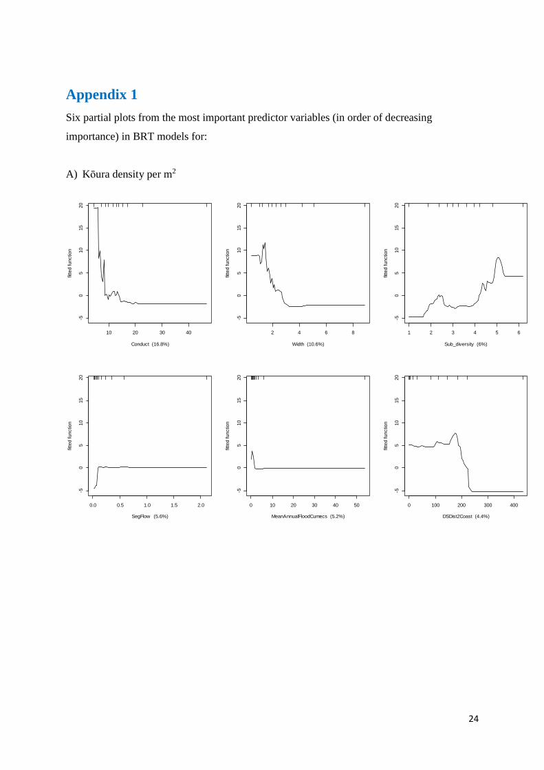
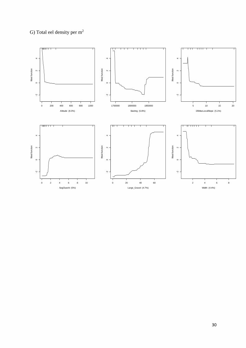
Appendix 1

Six partial plots from the most important predictor variables (in order of decreasing

importance) in BRT models for:

A) Kōura density per m2

10 20 30 40

-50

510

15

20

Conduct (16.8%)

fitte

d functio

n

2 4 6 8

-50

510

15

20

Width (10.6%)

fitte

d functio

n

1 2 3 4 5 6

-50

510

15

20

Sub_diversity (6%)

fitte

d functio

n

0.0 0.5 1.0 1.5 2.0

-50

510

15

20

SegFlow (5.6%)

fitte

d functio

n

0 10 20 30 40 50

-50

510

15

20

MeanAnnualFloodCumecs (5.2%)

fitte

d functio

n

0 100 200 300 400

-50

510

15

20

DSDist2Coast (4.4%)

fitte

d functio

n

25

B) Echyridella menziesii density per m2

0.0 0.2 0.4 0.6 0.8

-0.4

-0.2

0.0

0.2

GOBHUT (11.9%)

fitte

d functio

n

0 20 40 60 80 100-0

.4-0

.20.0

0.2

MeanAnnualFloodCumecs (11.4%)

fitte

d functio

n

0 5 10 15 20

-0.4

-0.2

0.0

0.2

Large_Wood (9.8%)

fitte

d functio

n

0e+00 1e+08 2e+08 3e+08 4e+08

-0.4

-0.2

0.0

0.2

CATCHAREA (8.3%)

fitte

d functio

n

5 10 15

-0.4

-0.2

0.0

0.2

Sediment_Depstn (7.7%)

fitte

d functio

n

1.0 1.5 2.0 2.5

-0.4

-0.2

0.0

0.2

USCalcium (7.6%)

fitte

d functio

n

26

C) Echyridella aucklandica density per m2

12 14 16 18 20 22 24

-0.1

0-0

.05

0.0

00.0

50.1

0

Temperature (21.7%)

fitte

d functio

n

2 4 6 8 10 12

-0.1

0-0

.05

0.0

00.0

50.1

0

DSMaxLocal (17.7%)

fitte

d functio

n

0 20 40 60 80 100

-0.1

0-0

.05

0.0

00.0

50.1

0

MeanAnnualFloodCumecs (15.9%)

fitte

d functio

n

0e+00 1e+08 2e+08 3e+08 4e+08

-0.1

0-0

.05

0.0

00.0

50.1

0

CATCHAREA (8.5%)

fitte

d functio

n

0 5 10 15 20 25

-0.1

0-0

.05

0.0

00.0

50.1

0

SEDE (6.5%)

fitte

d functio

n

0 5 10 15

-0.1

0-0

.05

0.0

00.0

50.1

0

WidthMALF (6.4%)

fitte

d functio

n

27

D) Total mussel density per m2

0.0 0.2 0.4 0.6 0.8

-0.6

-0.4

-0.2

0.0

0.2

0.4

GOBHUT (14.7%)

fitte

d functio

n

0 20 40 60 80 100

-0.6

-0.4

-0.2

0.0

0.2

0.4

MeanAnnualFloodCumecs (13.3%)

fitte

d functio

n

12 14 16 18 20 22 24

-0.6

-0.4

-0.2

0.0

0.2

0.4

Temperature (10%)

fitte

d functio

n

0e+00 1e+08 2e+08 3e+08 4e+08

-0.6

-0.4

-0.2

0.0

0.2

0.4

CATCHAREA (9.1%)

fitte

d functio

n

0 5 10 15 20

-0.6

-0.4

-0.2

0.0

0.2

0.4

Large_Wood (8.1%)

fitte

d functio

n

0 5 10 15

-0.6

-0.4

-0.2

0.0

0.2

0.4

WidthMALF (6.3%)

fitte

d functio

n

28

E) Shortfin eel density per m2

5 10 15 20

-20

24

6

DSMaxLocalSlope (11.1%)

fitte

d functio

n

0 200 400 600 800 1000-2

02

46

Altitude (6.8%)

fitte

d functio

n

0.0 0.2 0.4 0.6 0.8

-20

24

6

SegRipShade (5%)

fitte

d functio

n

1.0 1.5 2.0 2.5

-20

24

6

USCalcium (4.7%)

fitte

d functio

n

1750000 1800000 1850000

-20

24

6

Easting (4.5%)

fitte

d functio

n

1 2 3 4 5 6

-20

24

6

Sub_diversity (4.5%)

fitte

d functio

n

29

F) Longfin eel density per m2

1750000 1800000 1850000

02

46

Easting (30.7%)

fitte

d functio

n

0 1 2 3 4 5

02

46

Gradient (10.1%)

fitte

d functio

n

1.0 1.5 2.0 2.5

02

46

SegSlopeSqrt (7.4%)

fitte

d functio

n

2 4 6 8

02

46

Width (6.5%)

fitte

d functio

n

6 8 10 12 14 16 18 20

02

46

FRE3 (3.7%)

fitte

d functio

n

0.0e+00 5.0e+07 1.0e+08 1.5e+08 2.0e+08

02

46

usArea (3.7%)

fitte

d functio

n

30

G) Total eel density per m2

0 200 400 600 800 1000

-20

24

Altitude (8.3%)

fitte

d functio

n

1750000 1800000 1850000-2

02

4

Easting (5.8%)

fitte

d functio

n

5 10 15 20

-20

24

DSMaxLocalSlope (5.1%)

fitte

d functio

n

0 2 4 6 8 10

-20

24

SegCluesN (5%)

fitte

d functio

n

0 20 40 60

-20

24

Large_Gravel (4.7%)

fitte

d functio

n

2 4 6 8

-20

24

Width (4.4%)

fitte

d functio

n

31

H) Shortfin eel total biomass per m2

70 80 90 100 110 120 130 140

-10

12

MCI_State (11.2%)

fitte

d functio

n

0 20 40 60 80 100 120

-10

12

DO_perc (6.3%)

fitte

d functio

n

0 2 4 6 8 10

-10

12

SegCluesN (5.7%)

fitte

d functio

n

0.1 0.2 0.3 0.4 0.5 0.6 0.7

-10

12

Depth (5.6%)

fitte

d functio

n

0 20 40 60 80 100

-10

12

SEDO (5.5%)

fitte

d functio

n

0.0 0.5 1.0 1.5

-10

12

NO3N_State (3.7%)

fitte

d functio

n

32

I) Longfin eel total biomass per m2

0 50 100 150

-10

-50

5

Koura_den (20.5%)

fitte

d functio

n

2 4 6 8-1

0-5

05

Width (9.1%)

fitte

d functio

n

0 10 20 30 40

-10

-50

5

Channel_Width (5.8%)

fitte

d functio

n

2009 2010 2011 2012 2013 2014 2015 2016

-10

-50

5

Sample_year (3.4%)

fitte

d functio

n

0.1 0.2 0.3 0.4 0.5

-10

-50

5

SegFlow Variability (2.8%)

fitte

d functio

n

1 2 3 4 5 6

-10

-50

5

Sub_diversity (2.8%)

fitte

d functio

n

33

J) Shortfin eel biomass per individual fish

0.0 0.2 0.4 0.6 0.8

-10

12

3

SegLow Flow (16.8%)

fitte

d functio

n

0 10 20 30 40 50-1

01

23

MeanAnnualFloodCumecs (15.1%)

fitte

d functio

n

0 20 40 60 80 100

-10

12

3

SEDO (12.3%)

fitte

d functio

n

0 20 40 60 80 100

-10

12

3

Emergent_.exotic (6.5%)

fitte

d functio

n

0.02 0.04 0.06 0.08 0.10

-10

12

3

TP_State (5.6%)

fitte

d functio

n

0.1 0.2 0.3 0.4 0.5

-10

12

3

SegFlow Variability (5.5%)

fitte

d functio

n

34

K) Longfin eel biomass per individual fish

0 10 20 30 40 50 60 70

-8-6

-4-2

02

4

Bedrock (12.4%)

fitte

d functio

n

0.0 0.2 0.4 0.6 0.8-8

-6-4

-20

24

SegRipShade (8.6%)

fitte

d functio

n

0 100 200 300

-8-6

-4-2

02

4

Koura_abun (8.5%)

fitte

d functio

n

0 50 100 150

-8-6

-4-2

02

4

Koura_den (6.5%)

fitte

d functio

n

0 20 40 60

-8-6

-4-2

02

4

Large_Gravel (5.9%)

fitte

d functio

n

1 2 3 4 5 6

-8-6

-4-2

02

4

Sub_diversity (3.8%)

fitte

d functio

n