dss for integrated water resources management (iwrm) simulation based mc optimization ddr. kurt...
Post on 19-Dec-2015
217 views
TRANSCRIPT
DSS for Integrated DSS for Integrated Water Resources Water Resources
Management (IWRM)Management (IWRM)
DSS for Integrated DSS for Integrated Water Resources Water Resources
Management (IWRM)Management (IWRM)
Simulation based MC optimization
DDr. Kurt Fedra ESS GmbH, [email protected] http://www.ess.co.atEnvironmental Software & Services A-2352 Gumpoldskirchen
DDr. Kurt Fedra ESS GmbH, [email protected] http://www.ess.co.atEnvironmental Software & Services A-2352 Gumpoldskirchen
2
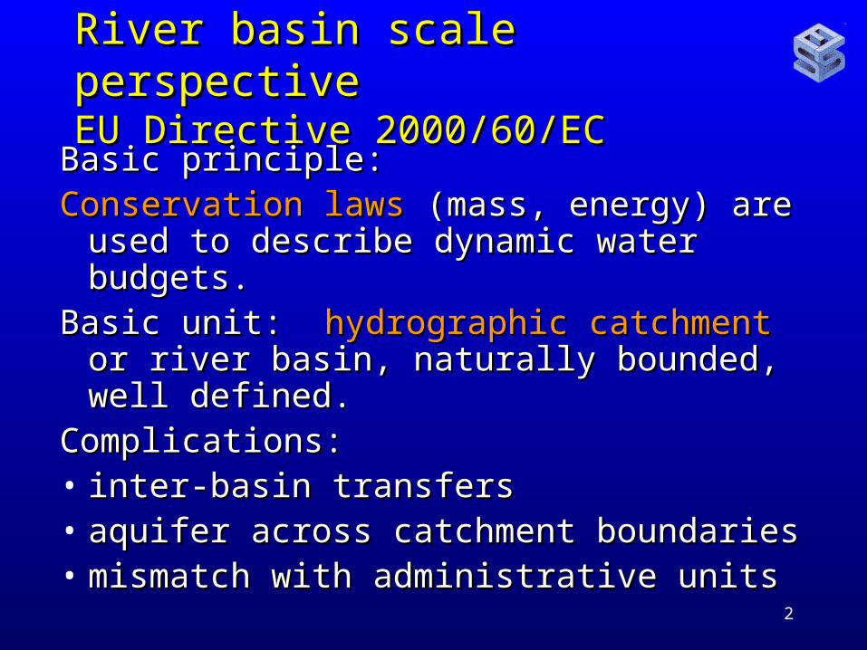
River basin scale perspectiveRiver basin scale perspective EU Directive 2000/60/ECEU Directive 2000/60/EC
Basic principle:Basic principle:Conservation lawsConservation laws (mass, energy) are used (mass, energy) are used
to describe dynamic water budgets.to describe dynamic water budgets.Basic unit: Basic unit: hydrographic catchmenthydrographic catchment or river or river
basin, naturally bounded, well defined.basin, naturally bounded, well defined.Complications: Complications: • inter-basin transfersinter-basin transfers• aquifer across catchment boundariesaquifer across catchment boundaries• mismatch with administrative unitsmismatch with administrative units
3
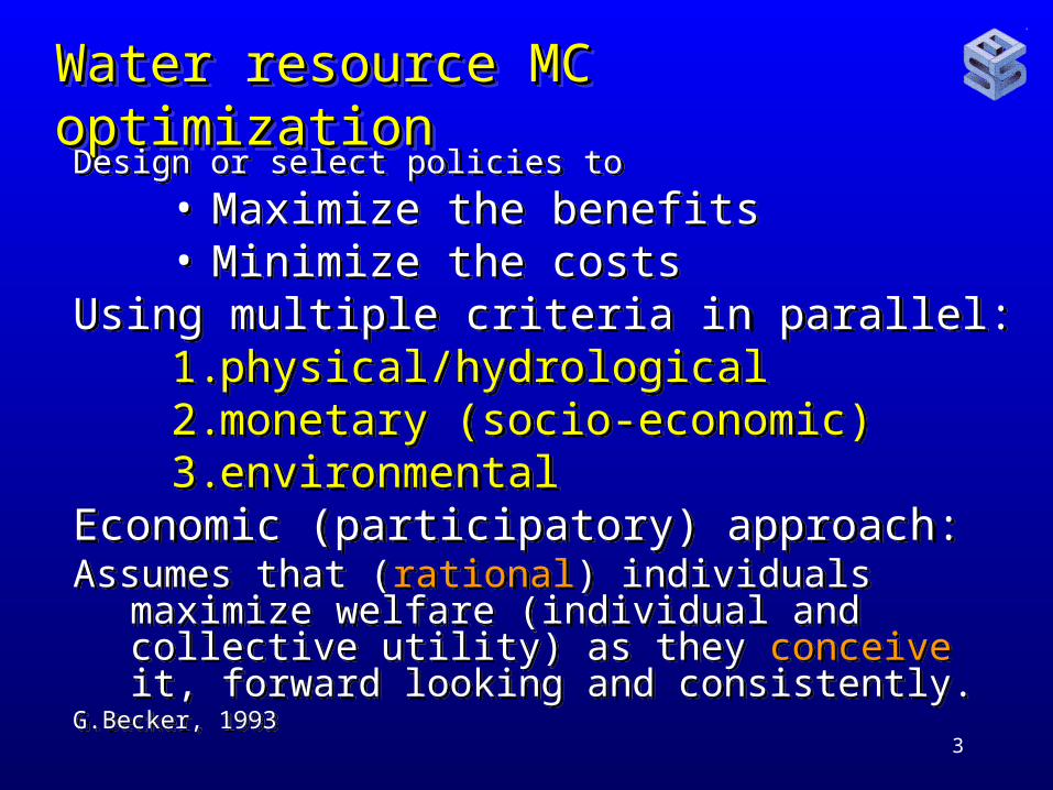
Water resource MC optimizationWater resource MC optimizationWater resource MC optimizationWater resource MC optimizationDesign or select policies to
• Maximize the benefits• Minimize the costs
Using multiple criteria in parallel:1.physical/hydrological 2.monetary (socio-economic) 3.environmental
Economic (participatory) approach:Assumes that (rational) individuals maximize
welfare (individual and collective utility) as they conceive it, forward looking and consistently.
G.Becker, 1993
Design or select policies to
• Maximize the benefits• Minimize the costs
Using multiple criteria in parallel:1.physical/hydrological 2.monetary (socio-economic) 3.environmental
Economic (participatory) approach:Assumes that (rational) individuals maximize
welfare (individual and collective utility) as they conceive it, forward looking and consistently.
G.Becker, 1993
4
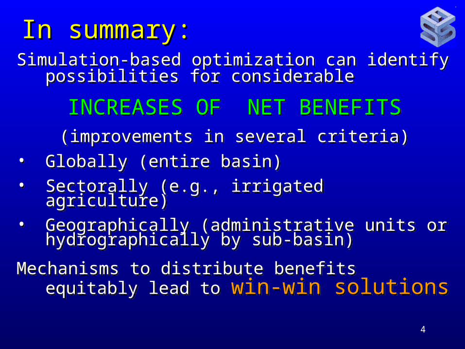
In summary:In summary:Simulation-based optimization can identify
possibilities for considerable
INCREASES OF NET BENEFITS (improvements in several criteria)
• Globally (entire basin)• Sectorally (e.g., irrigated agriculture)• Geographically (administrative units or
hydrographically by sub-basin)
Mechanisms to distribute benefits equitably lead to win-win solutions
Simulation-based optimization can identify possibilities for considerable
INCREASES OF NET BENEFITS (improvements in several criteria)
• Globally (entire basin)• Sectorally (e.g., irrigated agriculture)• Geographically (administrative units or
hydrographically by sub-basin)
Mechanisms to distribute benefits equitably lead to win-win solutions
5
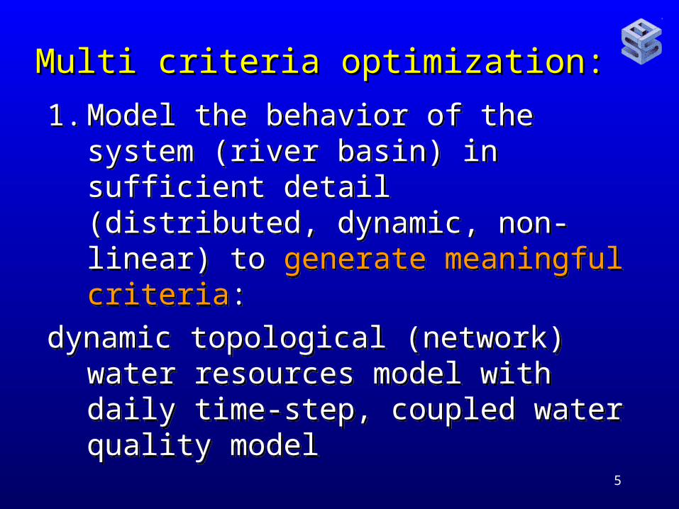
Multi criteria optimization:Multi criteria optimization:
1. Model the behavior of the system (river basin) in sufficient detail (distributed, dynamic, non-linear) to generate meaningful criteria:
dynamic topological (network) water resources model with daily time-step, coupled water quality model
1. Model the behavior of the system (river basin) in sufficient detail (distributed, dynamic, non-linear) to generate meaningful criteria:
dynamic topological (network) water resources model with daily time-step, coupled water quality model
6
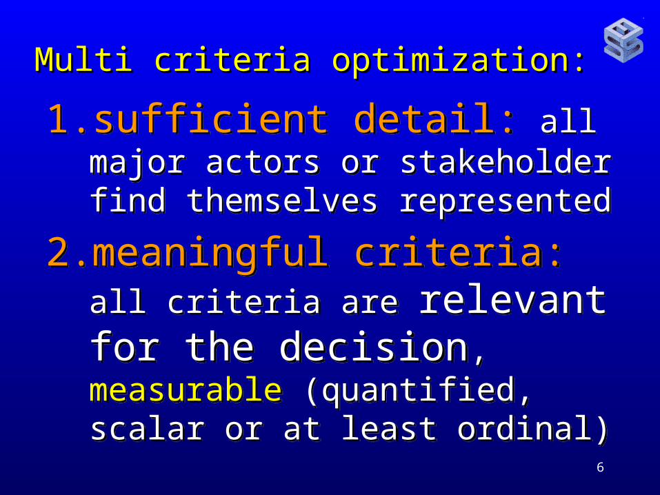
Multi criteria optimization:Multi criteria optimization:
1. sufficient detail: all major actors or stakeholder find themselves represented
2. meaningful criteria: all criteria
are relevant for the decision, measurable (quantified, scalar or at least ordinal)
1. sufficient detail: all major actors or stakeholder find themselves represented
2. meaningful criteria: all criteria
are relevant for the decision, measurable (quantified, scalar or at least ordinal)
7
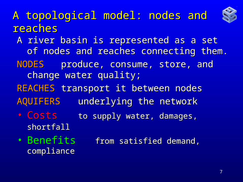
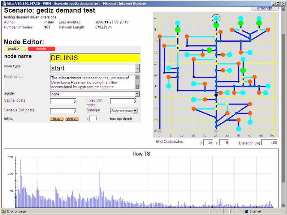
A topological model: nodes and reachesA topological model: nodes and reaches
A river basin is represented as a set of nodes and reaches connecting them.
NODES produce, consume, store, and change water quality;
REACHES transport it between nodes
AQUIFERS underlying the network
• Costs to supply water, damages, shortfall
• Benefits from satisfied demand, compliance
A river basin is represented as a set of nodes and reaches connecting them.
NODES produce, consume, store, and change water quality;
REACHES transport it between nodes
AQUIFERS underlying the network
• Costs to supply water, damages, shortfall
• Benefits from satisfied demand, compliance
8
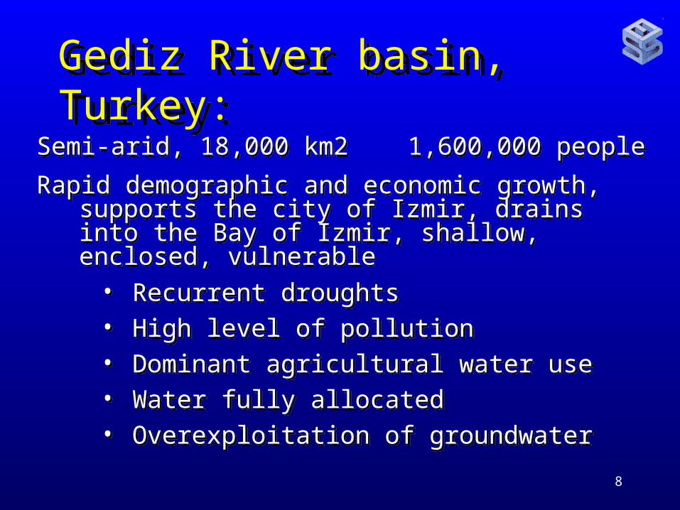
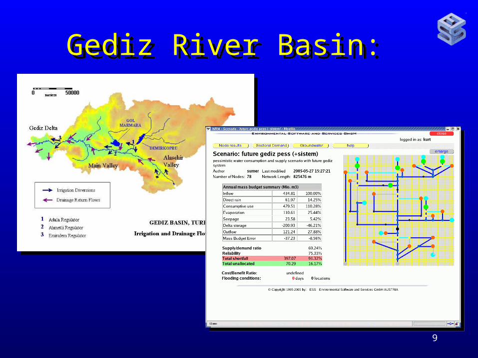
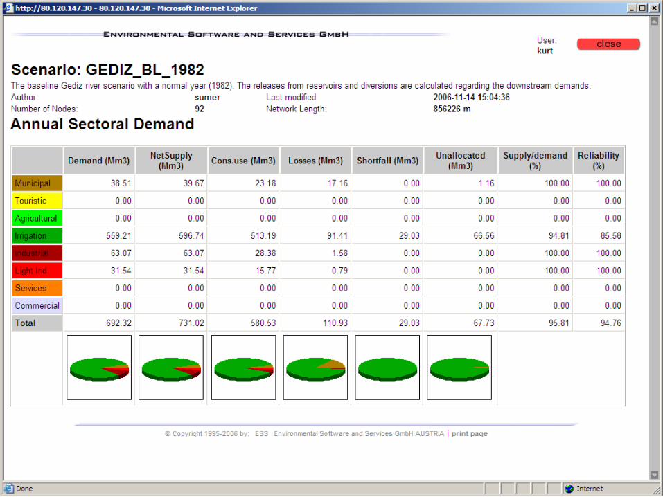
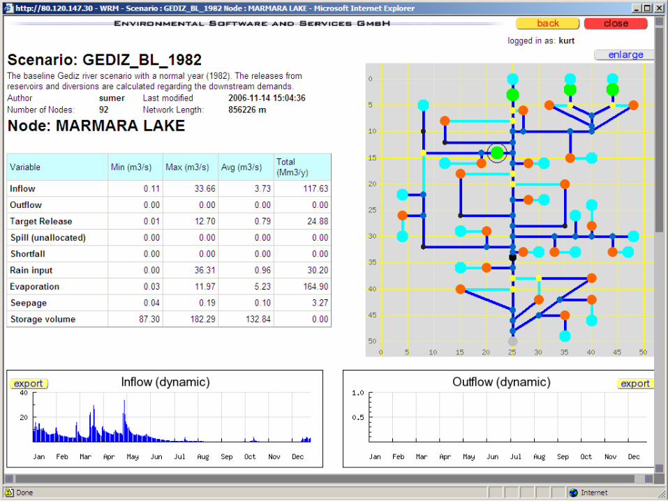
Gediz River basin, Turkey:Gediz River basin, Turkey:
Semi-arid, 18,000 km2 1,600,000 people
Rapid demographic and economic growth, supports the city of Izmir, drains into the Bay of Izmir, shallow, enclosed, vulnerable
• Recurrent droughts• High level of pollution• Dominant agricultural water use• Water fully allocated• Overexploitation of groundwater
9
Gediz River Basin:Gediz River Basin:
10
11
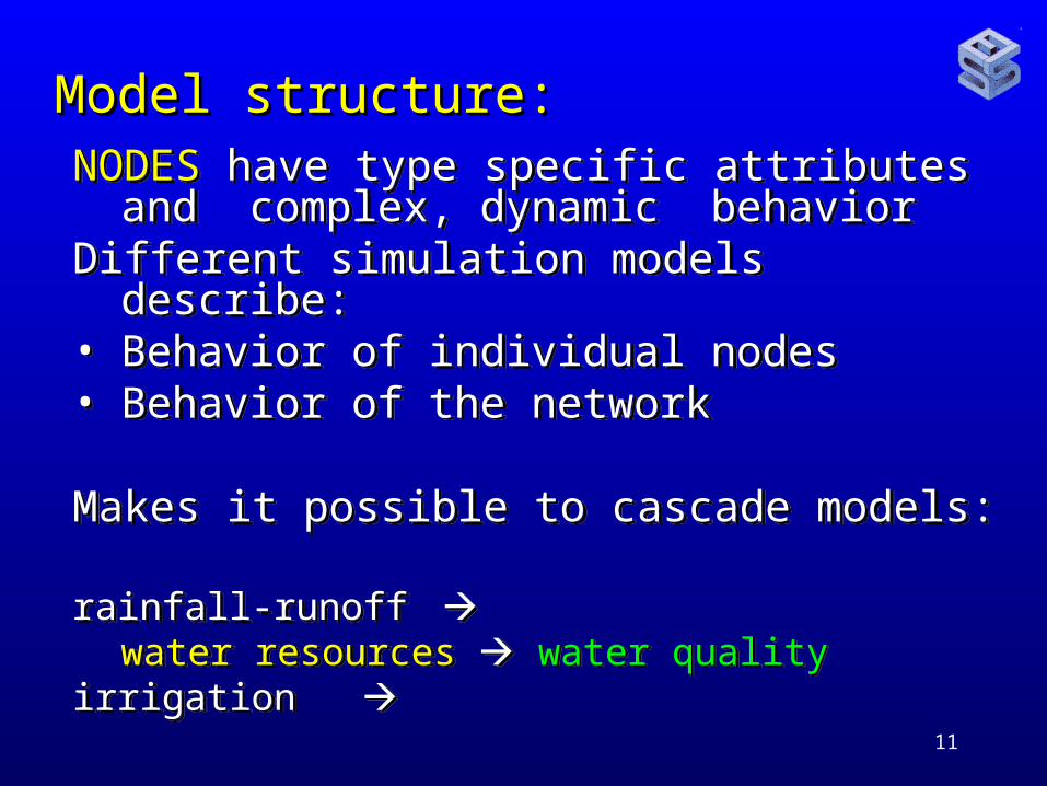
Model structure:Model structure:
NODES have type specific attributes and complex, dynamic behavior
Different simulation models describe: • Behavior of individual nodes• Behavior of the network
Makes it possible to cascade models:
rainfall-runoff water resources water quality
irrigation
NODES have type specific attributes and complex, dynamic behavior
Different simulation models describe: • Behavior of individual nodes• Behavior of the network
Makes it possible to cascade models:
rainfall-runoff water resources water quality
irrigation
12
13
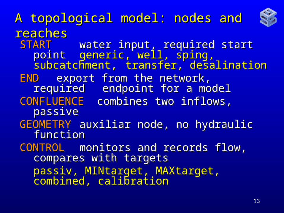
A topological model: nodes and reachesA topological model: nodes and reaches
START water input, required start point generic, well, sping,
subcatchment, transfer, desalination
END export from the network, required endpoint for a model
CONFLUENCE combines two inflows, passive GEOMETRY auxiliar node, no hydraulic
function CONTROL monitors and records flow,
compares with targetspassiv, MINtarget, MAXtarget,
combined, calibration
14
15
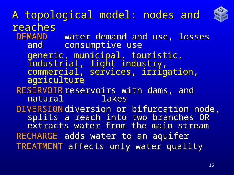
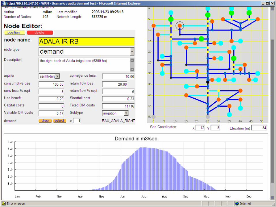
A topological model: nodes and reachesA topological model: nodes and reaches
DEMAND water demand and use, losses and consumptive use
generic, municipal, touristic, industrial, light industry,
commercial, services, irrigation, agriculture
RESERVOIR reservoirs with dams, and natural lakes
DIVERSIONdiversion or bifurcation node, splits a reach into two branches OR extracts water from the main stream
RECHARGE adds water to an aquifer TREATMENT affects only water quality
16
17
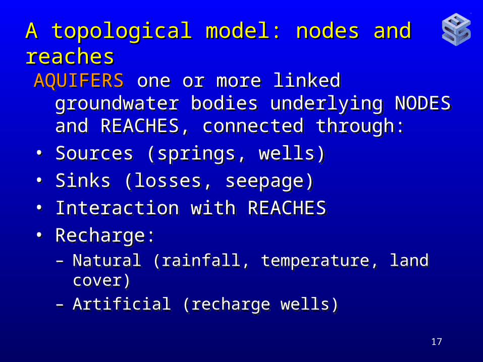
A topological model: nodes and reachesA topological model: nodes and reaches
AQUIFERS one or more linked groundwater bodies underlying NODES and REACHES, connected through:
• Sources (springs, wells)
• Sinks (losses, seepage)
• Interaction with REACHES
• Recharge: – Natural (rainfall, temperature, land cover)– Artificial (recharge wells)
AQUIFERS one or more linked groundwater bodies underlying NODES and REACHES, connected through:
• Sources (springs, wells)
• Sinks (losses, seepage)
• Interaction with REACHES
• Recharge: – Natural (rainfall, temperature, land cover)– Artificial (recharge wells)
18
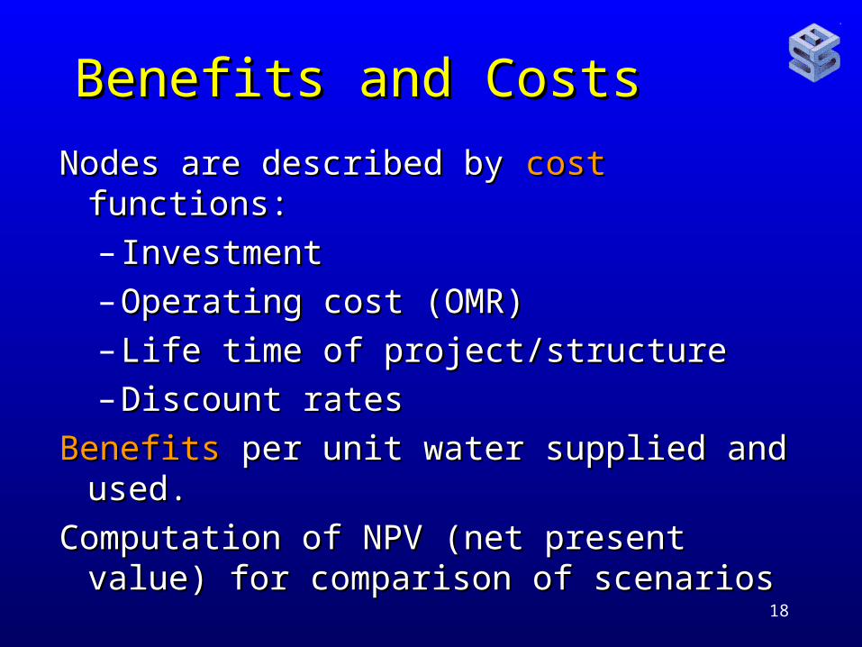
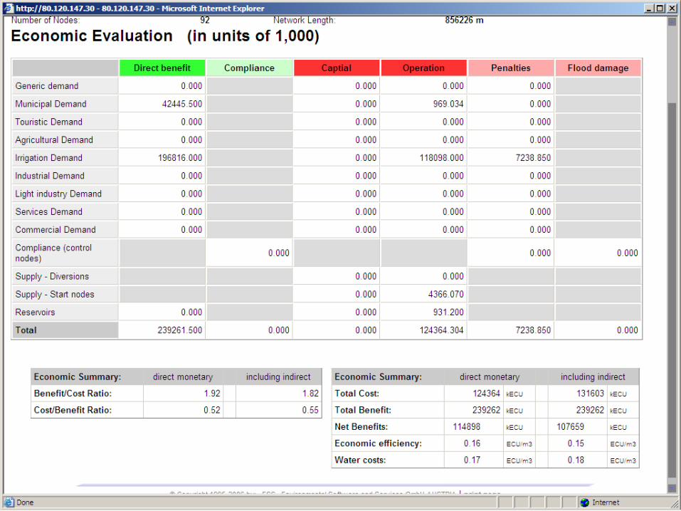
Benefits and CostsBenefits and Costs
Nodes are described by Nodes are described by cost cost functions:functions:
– InvestmentInvestment
– Operating cost (OMR)Operating cost (OMR)
– Life time of project/structureLife time of project/structure
– Discount ratesDiscount rates
BenefitsBenefits per unit water supplied and used. per unit water supplied and used.
Computation of NPV (net present value) for Computation of NPV (net present value) for comparison of scenarioscomparison of scenarios
19
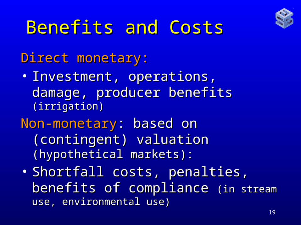
Benefits and CostsBenefits and Costs
Direct monetary:Direct monetary:• Investment, operations, damage, Investment, operations, damage,
producer benefits producer benefits (irrigation)(irrigation)
Non-monetaryNon-monetary: based on (contingent) : based on (contingent) valuation valuation (hypothetical markets):(hypothetical markets):
• Shortfall costs, penalties, benefits of Shortfall costs, penalties, benefits of compliance compliance (in stream use, environmental use)(in stream use, environmental use)
20
21
22
23
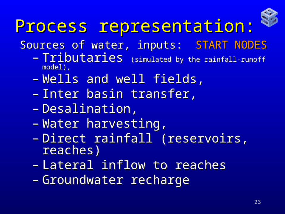
Process representation:Process representation:Sources of water, inputs: START NODES
– Tributaries (simulated by the rainfall-runoff model),
– Wells and well fields, – Inter basin transfer,– Desalination,– Water harvesting,– Direct rainfall (reservoirs, reaches)– Lateral inflow to reaches– Groundwater recharge
Sources of water, inputs: START NODES– Tributaries (simulated by the rainfall-runoff model),
– Wells and well fields, – Inter basin transfer,– Desalination,– Water harvesting,– Direct rainfall (reservoirs, reaches)– Lateral inflow to reaches– Groundwater recharge
24
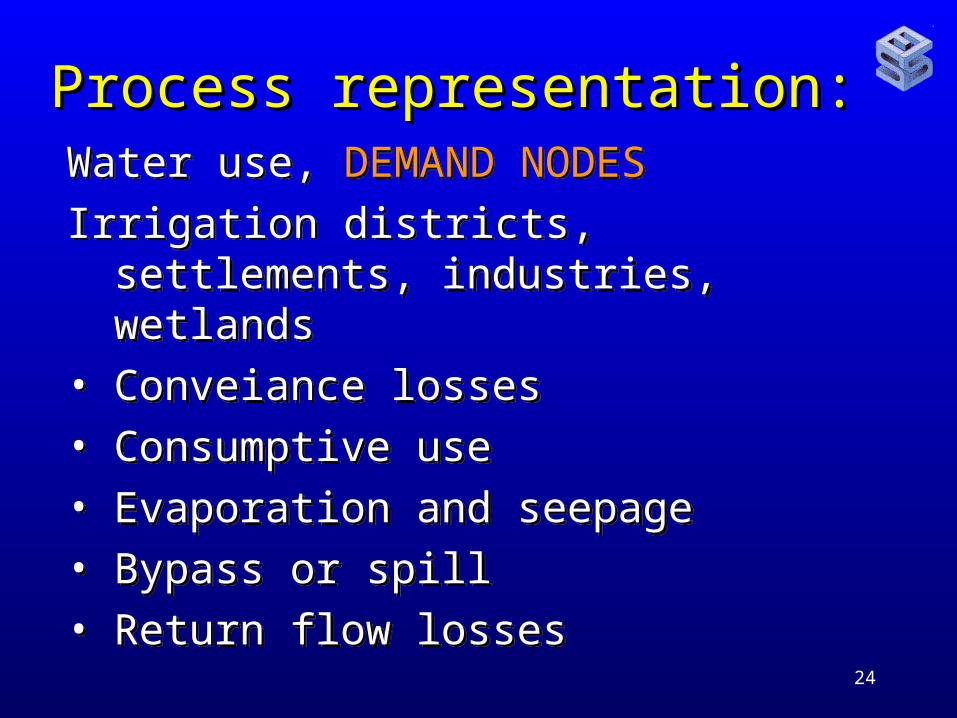
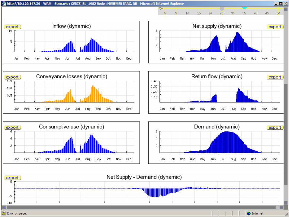
Process representation:Process representation:Water use, DEMAND NODES
Irrigation districts, settlements, industries, wetlands
• Conveiance losses
• Consumptive use
• Evaporation and seepage
• Bypass or spill
• Return flow losses
Water use, DEMAND NODES
Irrigation districts, settlements, industries, wetlands
• Conveiance losses
• Consumptive use
• Evaporation and seepage
• Bypass or spill
• Return flow losses
25
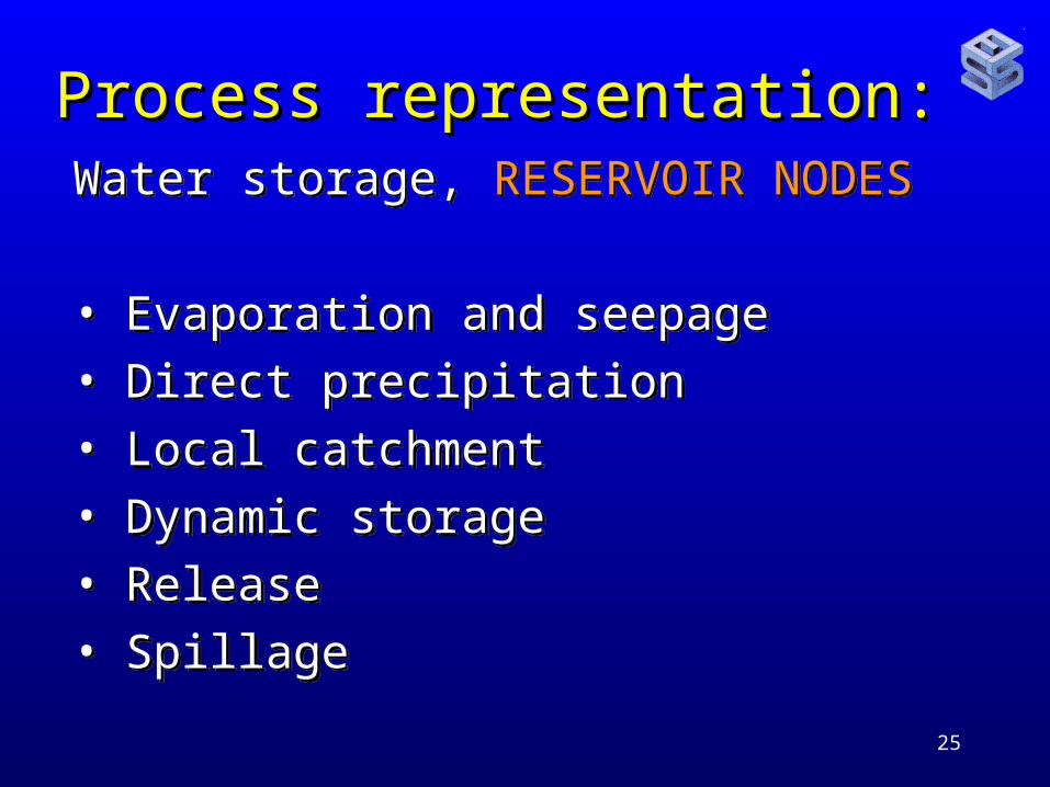
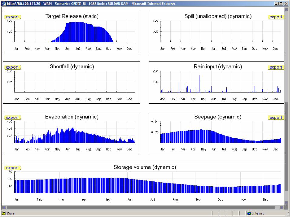
Process representation:Process representation:Water storage, RESERVOIR NODES
• Evaporation and seepage
• Direct precipitation
• Local catchment
• Dynamic storage
• Release
• Spillage
Water storage, RESERVOIR NODES
• Evaporation and seepage
• Direct precipitation
• Local catchment
• Dynamic storage
• Release
• Spillage
26
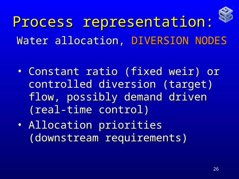
Process representation:Process representation:Water allocation, DIVERSION NODES
• Constant ratio (fixed weir) or controlled diversion (target) flow, possibly demand driven (real-time control)
• Allocation priorities (downstream requirements)
Water allocation, DIVERSION NODES
• Constant ratio (fixed weir) or controlled diversion (target) flow, possibly demand driven (real-time control)
• Allocation priorities (downstream requirements)

27
Process representation:Process representation:Flow constraints, CONTROL NODES
Constant or dynamic constraints:
• Minimum flow requirements
• Maximum flow: flooding (non-linear damage)
Flow constraints, CONTROL NODES
Constant or dynamic constraints:
• Minimum flow requirements
• Maximum flow: flooding (non-linear damage)
28
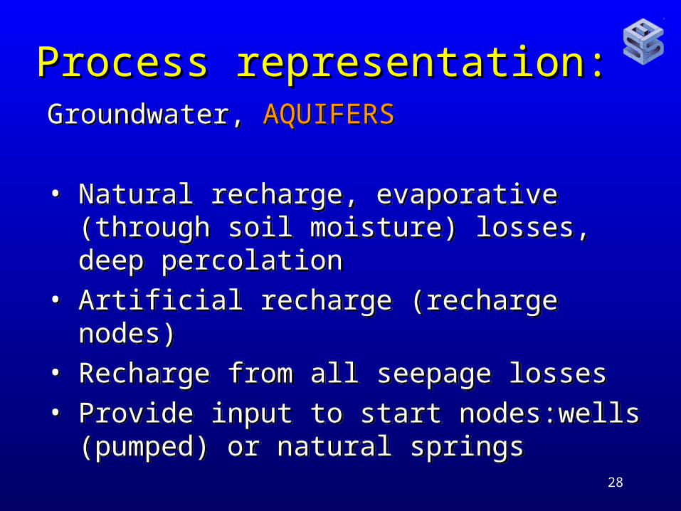
Process representation:Process representation:Groundwater, AQUIFERS
• Natural recharge, evaporative (through soil moisture) losses, deep percolation
• Artificial recharge (recharge nodes)
• Recharge from all seepage losses
• Provide input to start nodes:wells (pumped) or natural springs
Groundwater, AQUIFERS
• Natural recharge, evaporative (through soil moisture) losses, deep percolation
• Artificial recharge (recharge nodes)
• Recharge from all seepage losses
• Provide input to start nodes:wells (pumped) or natural springs
29
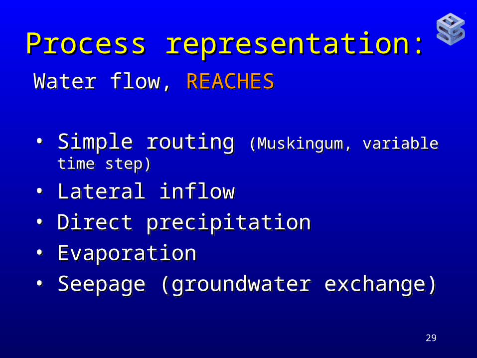
Process representation:Process representation:Water flow, REACHES
• Simple routing (Muskingum, variable time step)
• Lateral inflow
• Direct precipitation
• Evaporation
• Seepage (groundwater exchange)
Water flow, REACHES
• Simple routing (Muskingum, variable time step)
• Lateral inflow
• Direct precipitation
• Evaporation
• Seepage (groundwater exchange)
30
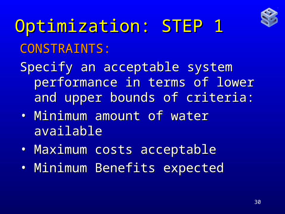
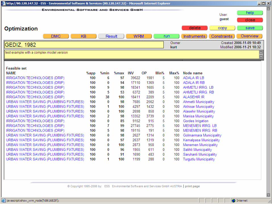
Optimization: STEP 1Optimization: STEP 1CONSTRAINTS:
Specify an acceptable system performance in terms of lower and upper bounds of criteria:
• Minimum amount of water available
• Maximum costs acceptable
• Minimum Benefits expected
CONSTRAINTS:
Specify an acceptable system performance in terms of lower and upper bounds of criteria:
• Minimum amount of water available
• Maximum costs acceptable
• Minimum Benefits expected
31
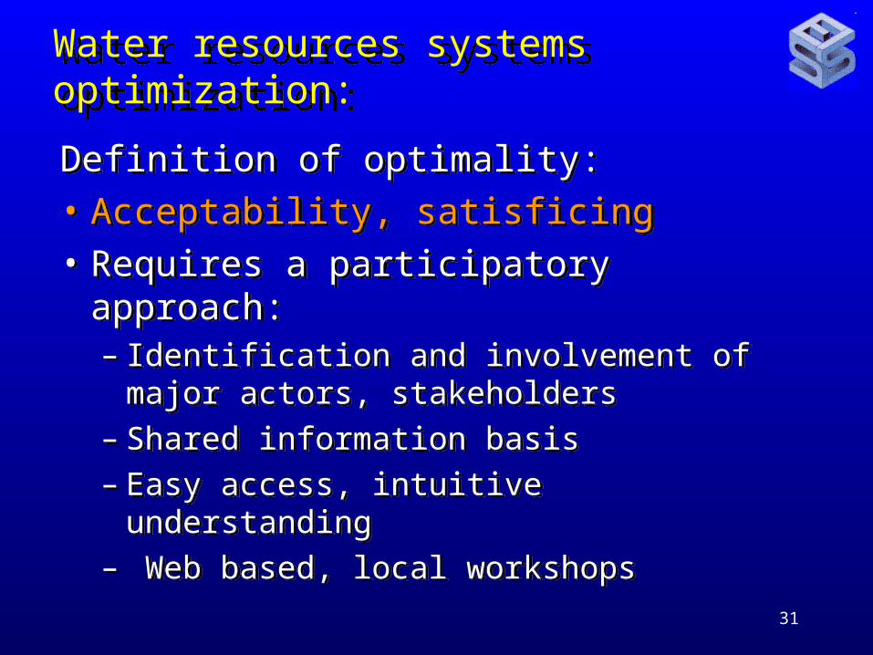
Water resources systems optimization:Water resources systems optimization:
Definition of optimality:
• Acceptability, satisficing
• Requires a participatory approach:– Identification and involvement of major
actors, stakeholders– Shared information basis– Easy access, intuitive understanding– Web based, local workshops
Definition of optimality:
• Acceptability, satisficing
• Requires a participatory approach:– Identification and involvement of major
actors, stakeholders– Shared information basis– Easy access, intuitive understanding– Web based, local workshops
32
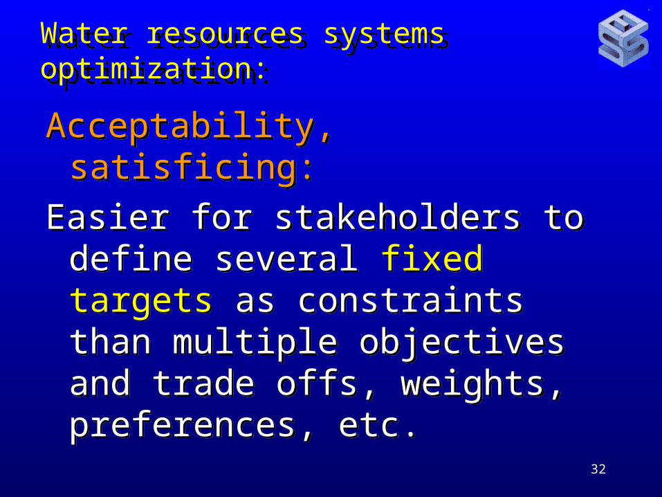
Water resources systems optimization:Water resources systems optimization:
Acceptability, satisficing:
Easier for stakeholders to define several fixed targets as constraints than multiple objectives and trade offs, weights, preferences, etc.
Acceptability, satisficing:
Easier for stakeholders to define several fixed targets as constraints than multiple objectives and trade offs, weights, preferences, etc.
33
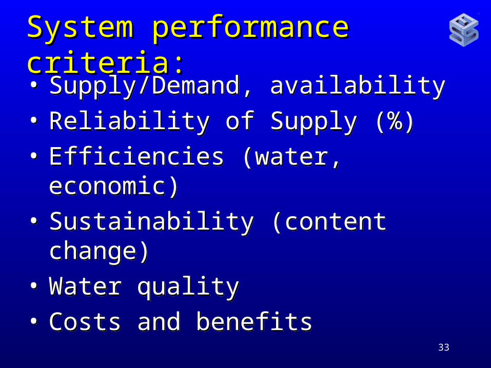
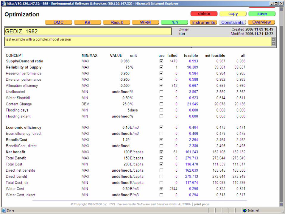
System performance criteria:System performance criteria:• Supply/Demand, availability
• Reliability of Supply (%)
• Efficiencies (water, economic)
• Sustainability (content change)
• Water quality
• Costs and benefits
• Supply/Demand, availability
• Reliability of Supply (%)
• Efficiencies (water, economic)
• Sustainability (content change)
• Water quality
• Costs and benefits

34
System performance criteria:System performance criteria:
• Diversion performance (%): the percentage of all "events" (summed over all diversion nodes and days) where the diversion target can be met;
• Allocation efficiency (%): the percentage of supply diverted to supply nodes that matches demands; all supply beyond demand is "wasted" and decreases allocation efficiency,
35
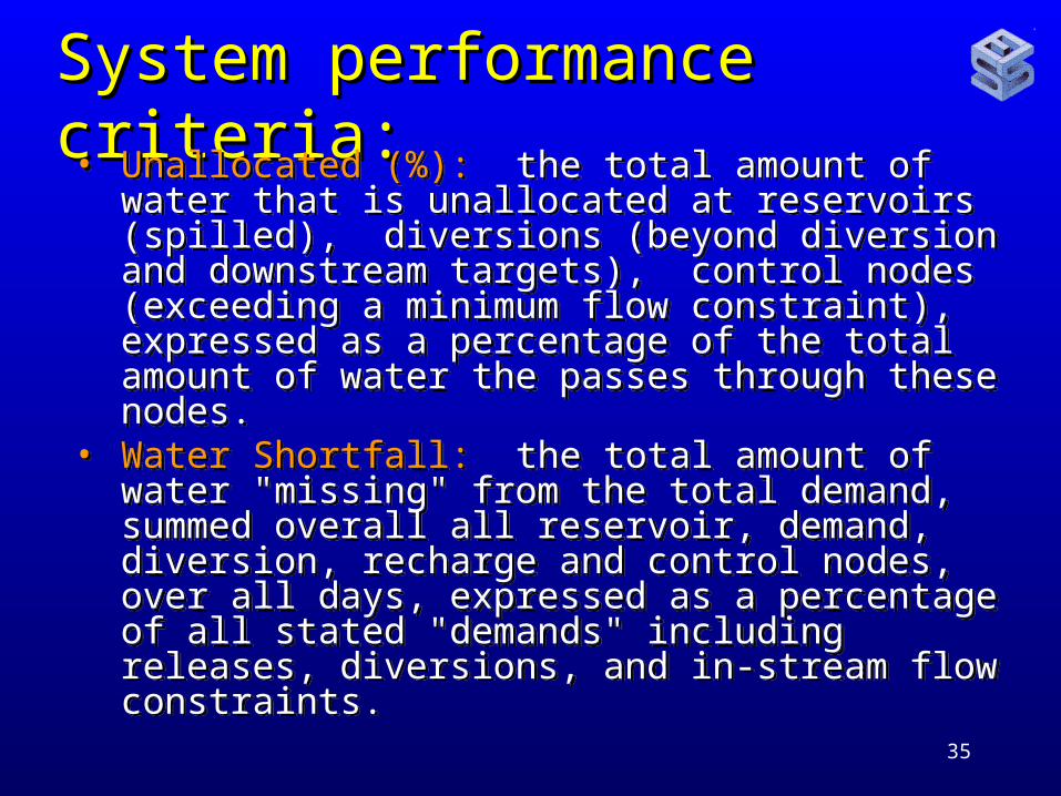
System performance criteria:System performance criteria:• Unallocated (%): the total amount of water that
is unallocated at reservoirs (spilled), diversions (beyond diversion and downstream targets), control nodes (exceeding a minimum flow constraint), expressed as a percentage of the total amount of water the passes through these nodes.
• Water Shortfall: the total amount of water "missing" from the total demand, summed overall all reservoir, demand, diversion, recharge and control nodes, over all days, expressed as a percentage of all stated "demands" including releases, diversions, and in-stream flow constraints.
• Unallocated (%): the total amount of water that is unallocated at reservoirs (spilled), diversions (beyond diversion and downstream targets), control nodes (exceeding a minimum flow constraint), expressed as a percentage of the total amount of water the passes through these nodes.
• Water Shortfall: the total amount of water "missing" from the total demand, summed overall all reservoir, demand, diversion, recharge and control nodes, over all days, expressed as a percentage of all stated "demands" including releases, diversions, and in-stream flow constraints.
36
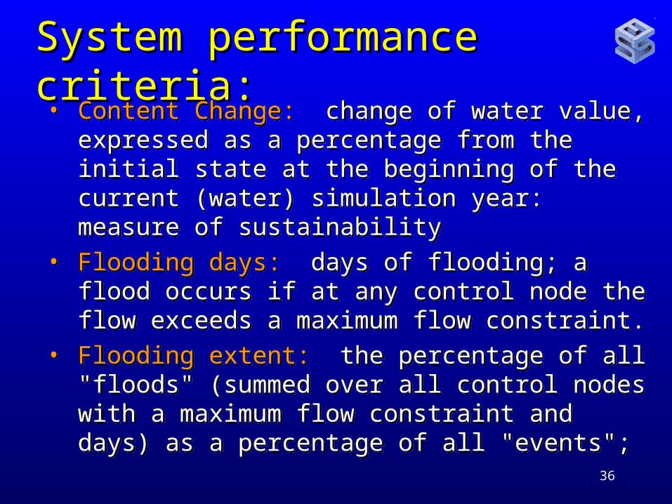
System performance criteria:System performance criteria:• Content Change: change of water value,
expressed as a percentage from the initial state at the beginning of the current (water) simulation year: measure of sustainability
• Flooding days: days of flooding; a flood occurs if at any control node the flow exceeds a maximum flow constraint.
• Flooding extent: the percentage of all "floods" (summed over all control nodes with a maximum flow constraint and days) as a percentage of all "events";
• Content Change: change of water value, expressed as a percentage from the initial state at the beginning of the current (water) simulation year: measure of sustainability
• Flooding days: days of flooding; a flood occurs if at any control node the flow exceeds a maximum flow constraint.
• Flooding extent: the percentage of all "floods" (summed over all control nodes with a maximum flow constraint and days) as a percentage of all "events";
37
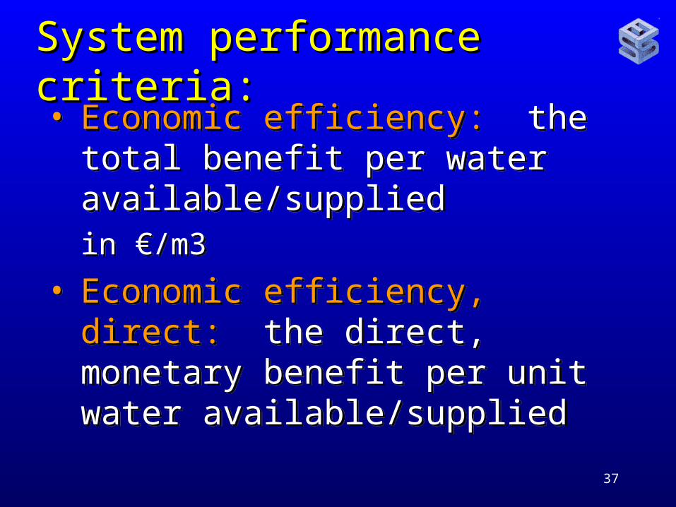
System performance criteria:System performance criteria:• Economic efficiency: the total benefit
per water available/supplied in €/m3
• Economic efficiency, direct: the direct, monetary benefit per unit water available/supplied
• Economic efficiency: the total benefit per water available/supplied in €/m3
• Economic efficiency, direct: the direct, monetary benefit per unit water available/supplied
38
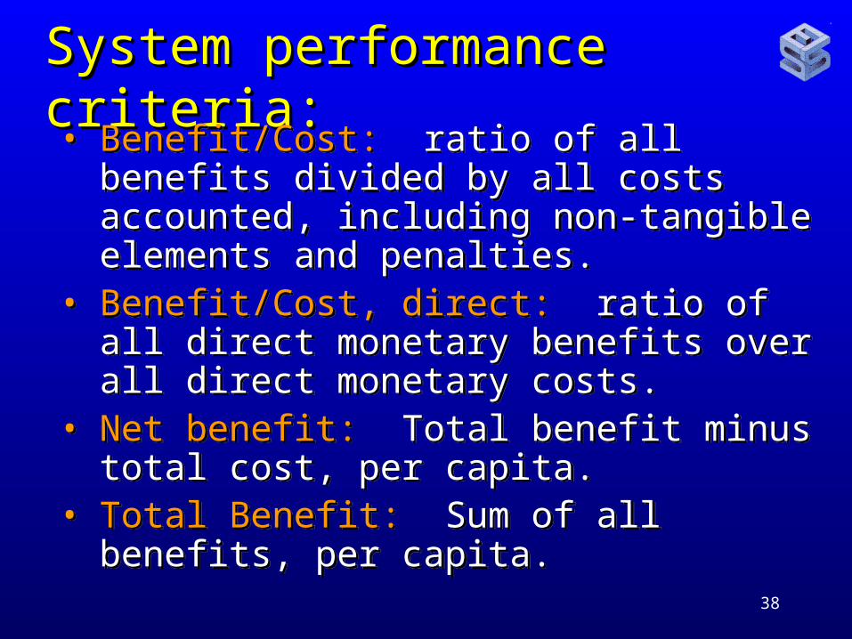
System performance criteria:System performance criteria:• Benefit/Cost: ratio of all benefits divided
by all costs accounted, including non-tangible elements and penalties.
• Benefit/Cost, direct: ratio of all direct monetary benefits over all direct monetary costs.
• Net benefit: Total benefit minus total cost, per capita.
• Total Benefit: Sum of all benefits, per capita.
• Benefit/Cost: ratio of all benefits divided by all costs accounted, including non-tangible elements and penalties.
• Benefit/Cost, direct: ratio of all direct monetary benefits over all direct monetary costs.
• Net benefit: Total benefit minus total cost, per capita.
• Total Benefit: Sum of all benefits, per capita.
39
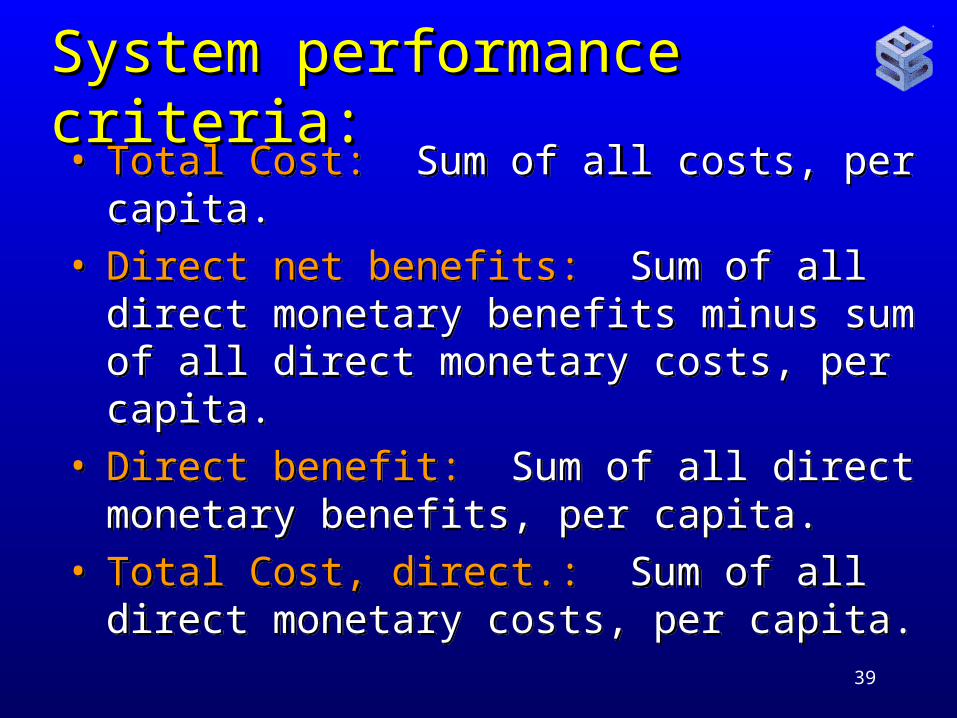
System performance criteria:System performance criteria:• Total Cost: Sum of all costs, per
capita. • Direct net benefits: Sum of all direct
monetary benefits minus sum of all direct monetary costs, per capita.
• Direct benefit: Sum of all direct monetary benefits, per capita.
• Total Cost, direct.: Sum of all direct monetary costs, per capita.
• Total Cost: Sum of all costs, per capita.
• Direct net benefits: Sum of all direct monetary benefits minus sum of all direct monetary costs, per capita.
• Direct benefit: Sum of all direct monetary benefits, per capita.
• Total Cost, direct.: Sum of all direct monetary costs, per capita.
40
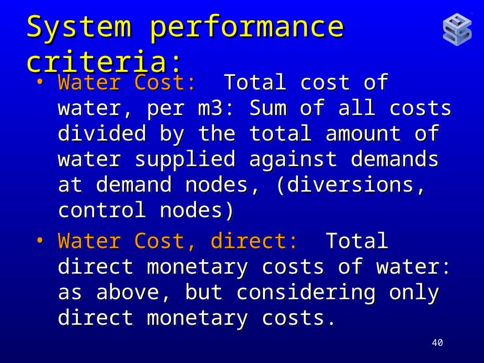
System performance criteria:System performance criteria:• Water Cost: Total cost of water, per m3:
Sum of all costs divided by the total amount of water supplied against demands at demand nodes, (diversions, control nodes)
• Water Cost, direct: Total direct monetary costs of water: as above, but considering only direct monetary costs.
• Water Cost: Total cost of water, per m3: Sum of all costs divided by the total amount of water supplied against demands at demand nodes, (diversions, control nodes)
• Water Cost, direct: Total direct monetary costs of water: as above, but considering only direct monetary costs.
41
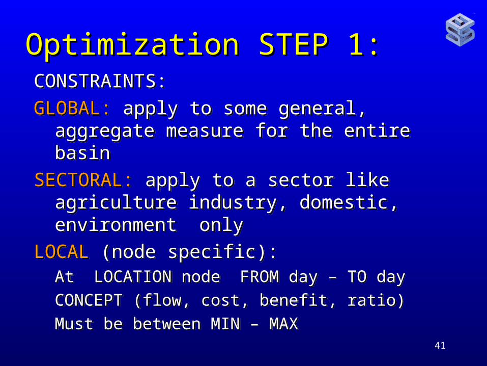
Optimization STEP 1:Optimization STEP 1:CONSTRAINTS:
GLOBAL: apply to some general, aggregate measure for the entire basin
SECTORAL: apply to a sector like agriculture industry, domestic, environment only
LOCAL (node specific):At LOCATION node FROM day – TO day
CONCEPT (flow, cost, benefit, ratio)
Must be between MIN – MAX
CONSTRAINTS:
GLOBAL: apply to some general, aggregate measure for the entire basin
SECTORAL: apply to a sector like agriculture industry, domestic, environment only
LOCAL (node specific):At LOCATION node FROM day – TO day
CONCEPT (flow, cost, benefit, ratio)
Must be between MIN – MAX
42
43
44
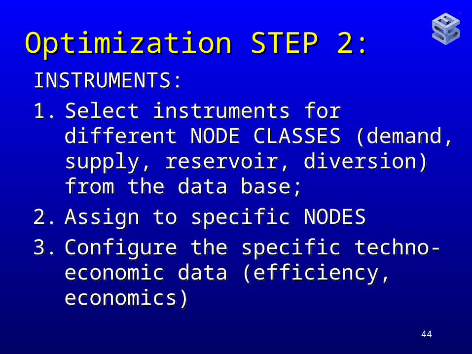
Optimization STEP 2:Optimization STEP 2:INSTRUMENTS:
1. Select instruments for different NODE CLASSES (demand, supply, reservoir, diversion) from the data base;
2. Assign to specific NODES
3. Configure the specific techno-economic data (efficiency, economics)
INSTRUMENTS:
1. Select instruments for different NODE CLASSES (demand, supply, reservoir, diversion) from the data base;
2. Assign to specific NODES
3. Configure the specific techno-economic data (efficiency, economics)

45
46
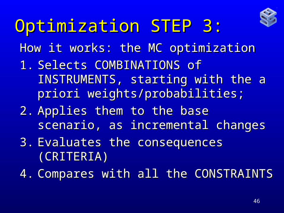
Optimization STEP 3:Optimization STEP 3:How it works: the MC optimization
1. Selects COMBINATIONS of INSTRUMENTS, starting with the a priori weights/probabilities;
2. Applies them to the base scenario, as incremental changes
3. Evaluates the consequences (CRITERIA)
4. Compares with all the CONSTRAINTS
How it works: the MC optimization
1. Selects COMBINATIONS of INSTRUMENTS, starting with the a priori weights/probabilities;
2. Applies them to the base scenario, as incremental changes
3. Evaluates the consequences (CRITERIA)
4. Compares with all the CONSTRAINTS
47
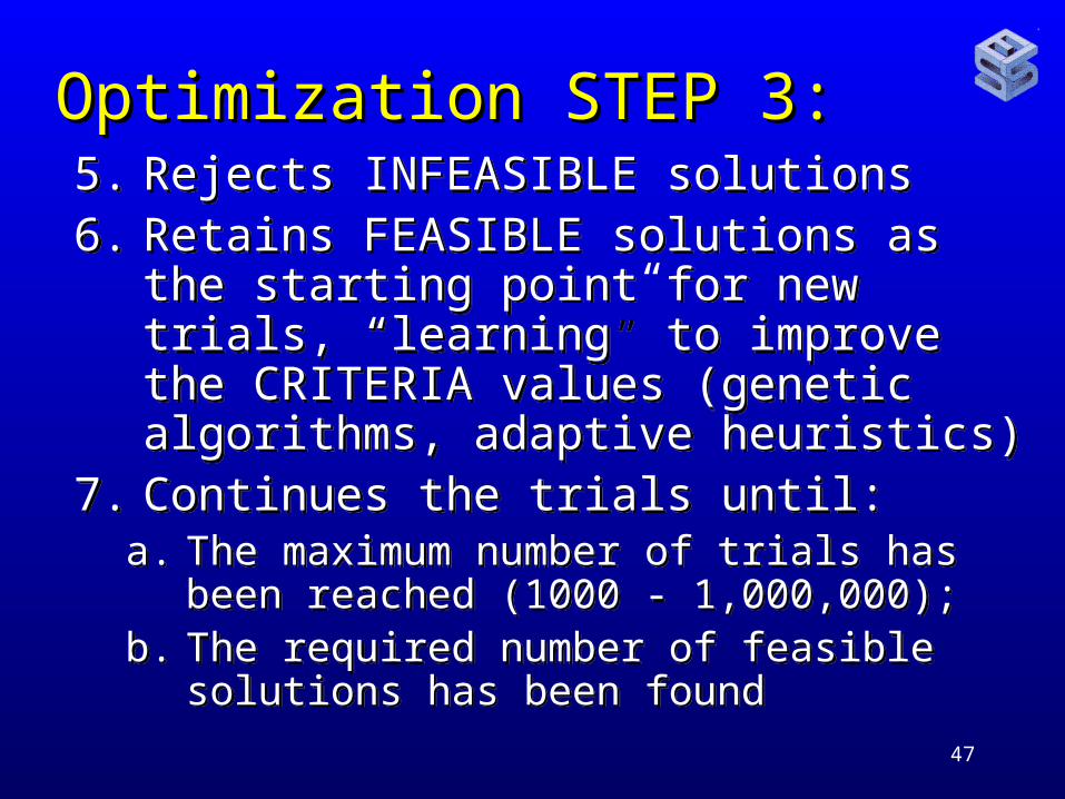
Optimization STEP 3:Optimization STEP 3:5. Rejects INFEASIBLE solutions6. Retains FEASIBLE solutions as the
starting point for new trials, “learning” to improve the CRITERIA values (genetic algorithms, adaptive heuristics)
7. Continues the trials until:a. The maximum number of trials has been
reached (1000 - 1,000,000);b. The required number of feasible solutions
has been found
5. Rejects INFEASIBLE solutions6. Retains FEASIBLE solutions as the
starting point for new trials, “learning” to improve the CRITERIA values (genetic algorithms, adaptive heuristics)
7. Continues the trials until:a. The maximum number of trials has been
reached (1000 - 1,000,000);b. The required number of feasible solutions
has been found
48
49
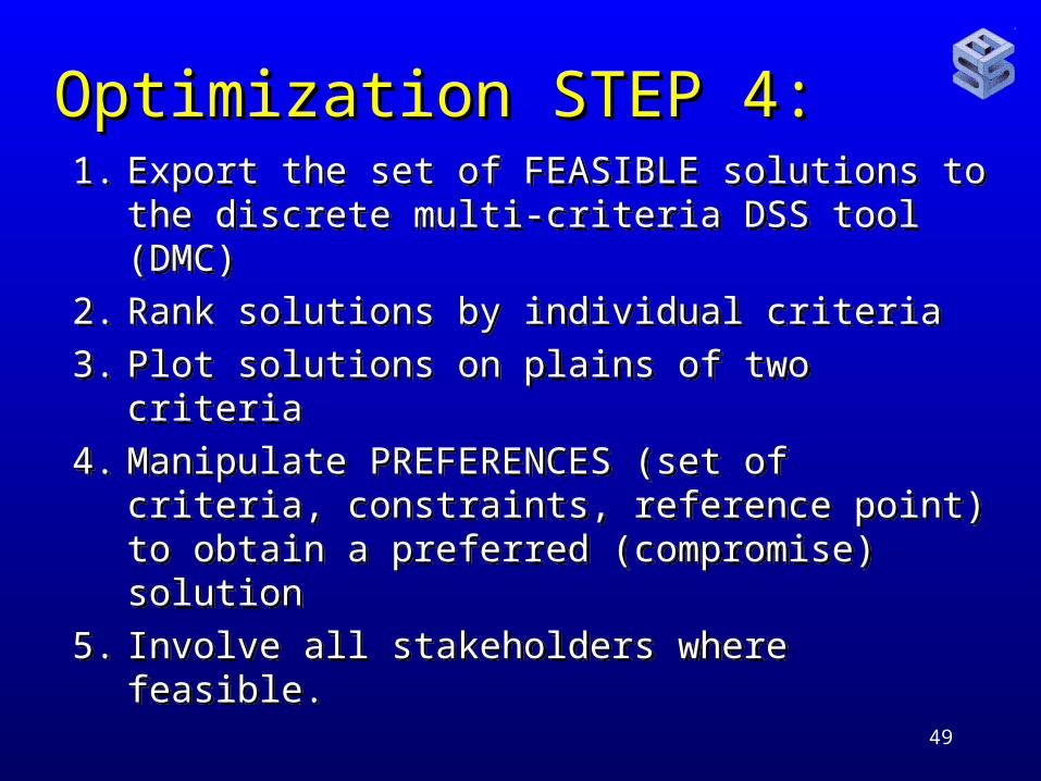
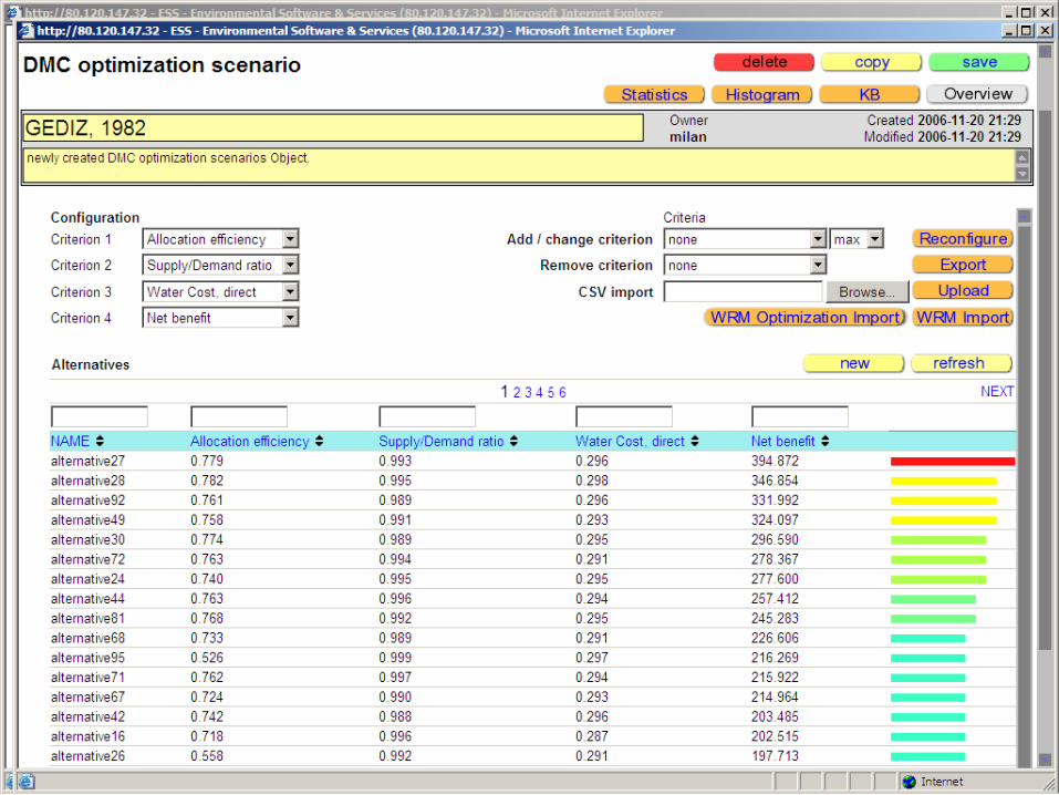
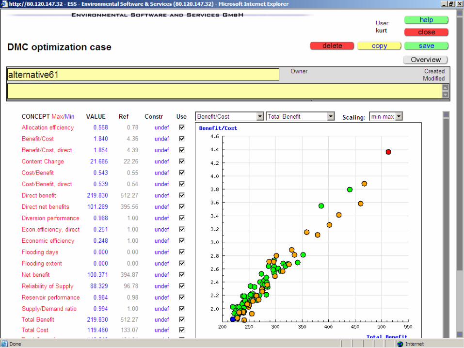
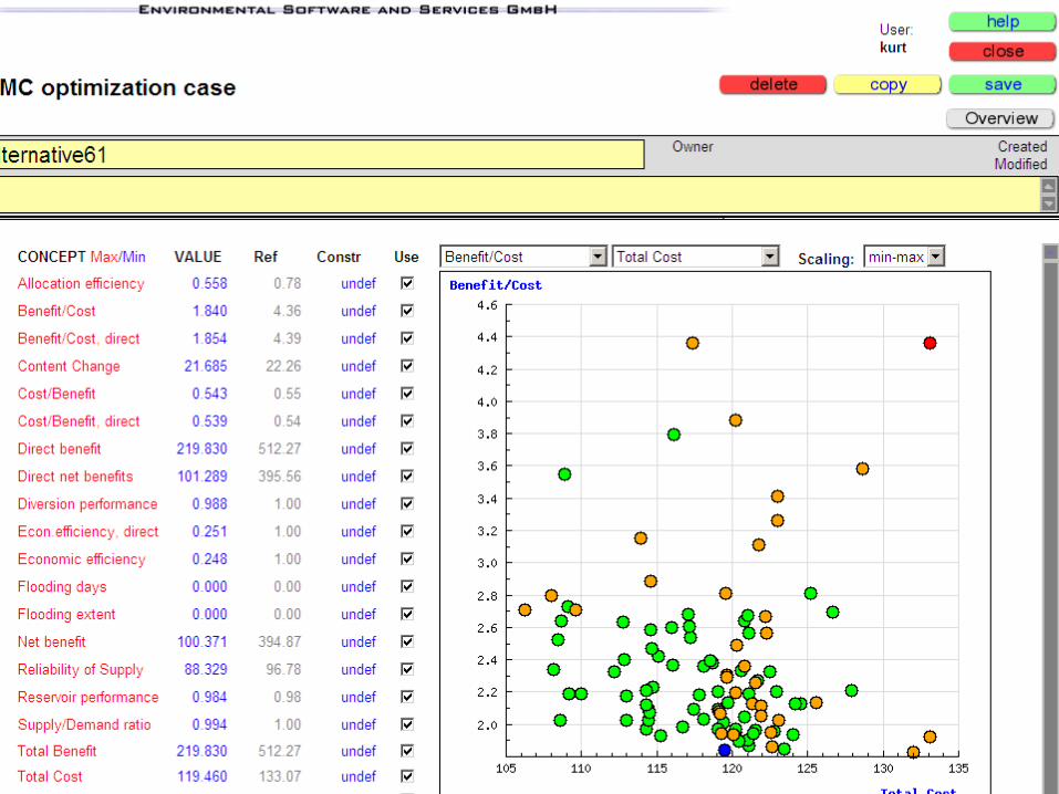
Optimization STEP 4:Optimization STEP 4:1. Export the set of FEASIBLE solutions to
the discrete multi-criteria DSS tool (DMC)
2. Rank solutions by individual criteria
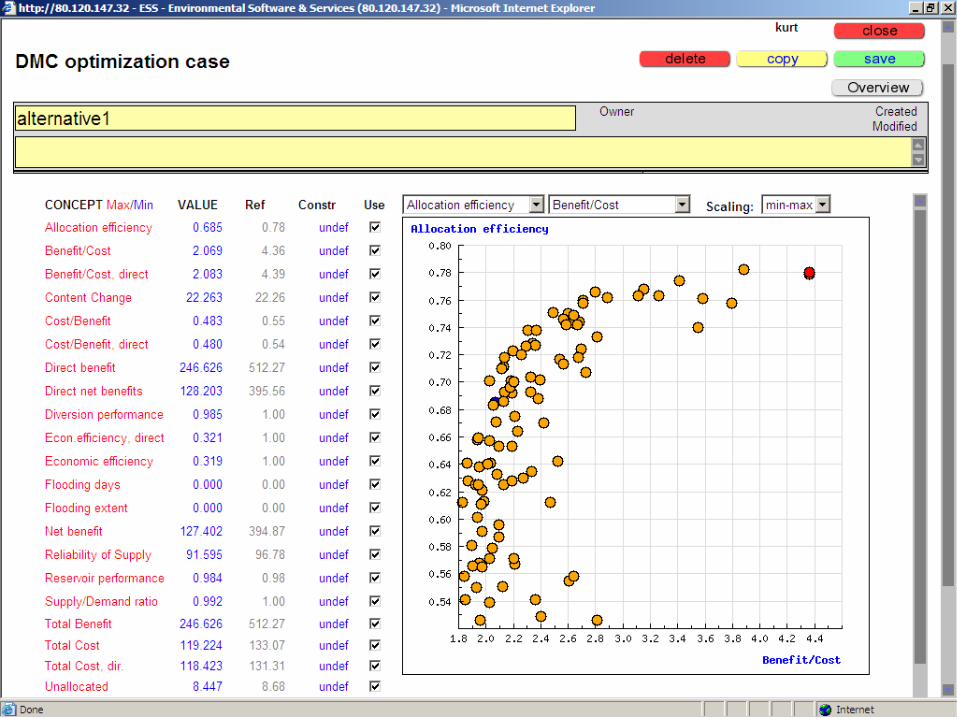
3. Plot solutions on plains of two criteria
4. Manipulate PREFERENCES (set of criteria, constraints, reference point) to obtain a preferred (compromise) solution
5. Involve all stakeholders where feasible.
1. Export the set of FEASIBLE solutions to the discrete multi-criteria DSS tool (DMC)
2. Rank solutions by individual criteria
3. Plot solutions on plains of two criteria
4. Manipulate PREFERENCES (set of criteria, constraints, reference point) to obtain a preferred (compromise) solution
5. Involve all stakeholders where feasible.
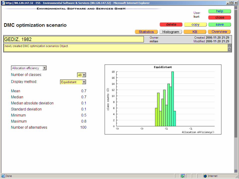
50
51
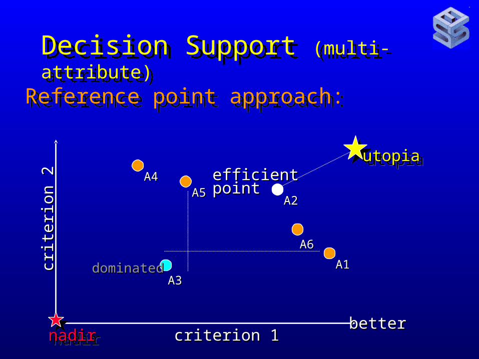
Decision Support (multi-attribute)Decision Support (multi-attribute)
Reference point approach:Reference point approach:
nadirnadirnadirnadir
utopiautopiautopiautopia
A1A1
A2A2
A3A3
A4A4
betterbetter
efficient efficient pointpoint
criterion 1criterion 1
crite
rion
2cr
iterio
n 2 A5A5
dominateddominated
A6A6
53
54
55
56
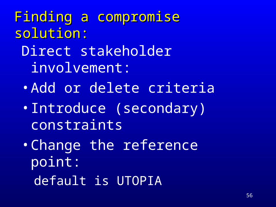
Finding a compromise solution:Finding a compromise solution:
Direct stakeholder involvement:
• Add or delete criteria
• Introduce (secondary) constraints
• Change the reference point: default is UTOPIA
57
58
59
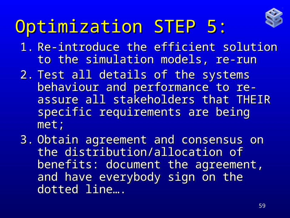
Optimization STEP 5:Optimization STEP 5:1. Re-introduce the efficient solution to the
simulation models, re-run2. Test all details of the systems behaviour
and performance to re-assure all stakeholders that THEIR specific requirements are being met;
3. Obtain agreement and consensus on the distribution/allocation of benefits: document the agreement, and have everybody sign on the dotted line….
1. Re-introduce the efficient solution to the simulation models, re-run
2. Test all details of the systems behaviour and performance to re-assure all stakeholders that THEIR specific requirements are being met;
3. Obtain agreement and consensus on the distribution/allocation of benefits: document the agreement, and have everybody sign on the dotted line….
60
61
62

63
In summary:In summary:Simulation-based optimization can identify
possibilities for considerable
INCREASES OF NET BENEFITS (improvements in several criteria)
• Globally (entire basin)• Sectorally (e.g., irrigated agriculture)• Geographically (administrative units or
hydrographically by sub-basin)
Mechanisms to distribute benefits equitably lead to win-win solutions
Simulation-based optimization can identify possibilities for considerable
INCREASES OF NET BENEFITS (improvements in several criteria)
• Globally (entire basin)• Sectorally (e.g., irrigated agriculture)• Geographically (administrative units or
hydrographically by sub-basin)
Mechanisms to distribute benefits equitably lead to win-win solutions