dynamic assessment of overhead line capacity for

[email protected]

Dynamic Assessment of Overhead Line Capacity for integrating Renewable Energy into the Transmission Grid

Sara FERNÁNDEZ DE SEVILLA, Gerardo GONZALEZ, Guillermo JUBERIAS, Luis MARTÍNEZ, Miguel ESCRIBANO, Javier IGLESIAS, Pablo ALBI, Unai BÚRDALO,

Álvaro MUÑÍZ, Sacha KWIK (REE, Spain)

SUMMARY The need for integrating new variable sources of energy into the grid requires more accurate assessment of the transmission capacity of overhead lines in a continuously changing environment. The conductor temperature is usually the factor that determines the transmission capacity of a line, in order to avoid excessive sags and possible damages in the materials. Hence, a proper control of the conductor temperature along the line and during time will help to maximize this capacity. The methods for Dynamic Line Rating have experienced an important development during the recent years. These methods need to properly relate the changes of the different parameters and variables of an overhead line during time, based on local measurements (typically wind speed, wind direction, solar radiation and ambient temperature). The use of continuous temperature measurement of the overhead conductor, using Optical Phase Conductor (OPPC), can help to validate these methods and develop the models to improve the performance of such systems. One of the demo projects belonging to the European Twenties project includes the innovative application of an OPPC conductor over an aerial power line combined with a set of weather stations. The aim is increasing the flexibility of the transmission grid by assessing the thermal behaviour of the line in a real changing environment. The continuous real time measurement of the temperature is achieved thanks to the implementation of a new data acquisition system by IP network that allows getting and registering the data instantaneously and with all devices synchronized. The temperature data and the weather stations measurements are processed by algorithms to determine the capacity of the line for different time intervals. These algorithms compare the thermal rating models with the data provided by the meteorological services, which are used for wind generation forecasting, in order to find a correlation between the thermal behaviour of the line and the nearby wind production capacity. The OPPC has been installed in the lower phase of a new 220 kV 30km double-circuit line in Spain (Fuendetodos-Maria) which connects several wind farms to the transmission grid. This technology has passed all the technical validation phases through simulations, lab testing and finally in the field demonstrating that the functionality aimed is successfully obtained. In this document we are showing a brief description of the installation made in the transmission grid, the measurements and the analysis of the results obtained. KEYWORDS Dynamic Line Ratings. Thermal Behaviour of Overhead Conductors. Transmission Line Capacity. OPPC Conductors. Integration of Wind Energy into the Transmission Grid.

21, rue d’Artois, F-75008 PARIS B2-207 CIGRE 2014 http : //www.cigre.org

1

INTRODUCTION This project is a large scale demonstration based on the idea that RTTR devices can help to increase the grid flexibility to support massive renewable integration. This demo was developed and leaded by Red Eléctrica (REE) and it was part of the TWENTIES R&D project. Nowadays the transmission capacity of an overhead line (OHL) is calculated according to static seasonal restrictions in the use of infrastructures without taking into account meteorological conditions which determines the real transmission capacity value. In this framework, the aim of this demo was to evaluate the real-time conductor temperature demonstrating that latent transmission capacity can exist in these lines directly involved in the evacuation of wind farms energy on a case-by-case basis. As a result, the dispatch control center can use this latent capacity to bring flexibility and expand the capability of the network, evacuating more energy with the current level of reliability performance. In this development, one sub-conductor was replaced by an optical phase power conductor (OPPC), in order to measure the thermal behavior of the conductors over entire line using a Distributed Temperature Sensor (DTS).

Figure 1: Project outline. Attachment tower

This large scale demonstration was carried out in a new 220 kV line Maria-Fuendetodos, commissioned on November 2012 and located in the region of Aragon (North-East of Spain). A 1730 MW wind power capacity is installed in this zone.

Figure 2: Location of the line

This paper is organised in the following sections:

2

Technical characteristics of the line: - General characteristics - OPPC characteristics - Accessories - Termination Unit - Straight-joints

Monitoring system: - General overview of the system - Temperature Monitoring System - Weather Stations - Communication system IP Network. - Central System - Control Center: Real Time Operation

Analysis of preliminary results: - Temperature variation - Gradient of temperature - Probability distribution of critical sections location - Analysis of the critical sections location - Dynamic rate behavior - Wind power correlation analysis

Conclusions TECHNICAL CHARACTERISTICS OF THE LINE General characteristics The general characteristics of the 220 kV Maria-Fuendetodos line are: - Rated voltage 220kV - Transmission Capacity Spring/Summer (static rating before demo) 790 / 730 MVA - Configuration Twin bundle - Maximum admissible temperature 85º C - Conductor type CONDOR ACSR/AW - Number of towers 86 - Number of anchoring towers 35% - Number of sections 31 - Total route length 29.917 meters - Total conductor length ~30.530 meters - Direction changes/angles 25

As mentioned before, one sub-conductor of the lower phase was replaced by an optical phase power conductor OPPC (395-AL1/53-A20SA), in order to measure the thermal behavior of the conductors over the complete line using a Distributed Temperature Sensing (DTS). It was chosen the lower phase not only to facilitate the assembly and laying processes, but also because this phase should be the most critical according to the mandatory safety clearances and could be less influenced by the favorable conditions withstood under windy days. OPPC characteristics The OPPC conductor includes 10 single-mode optical fibers (8 fibers G.652.D + 2 fibers G.655) inside a stainless steel tube (aluminum coated), located in the inner aluminum layer, close to the steel core of the cable. Only one of the G.655 fibers is currently in service.

3

Figure 3: OPPC real pictures

The OPPC was designed in accordance to EN 50182, EN 50152, UNE-EN-60889 and EN 61232. The allowable tolerances for the nominal wire diameters were specifically taken into consideration to meet the parameters of a Condor ACSR conductor as close as possible. The differences in sag between the ACSR and the OPPC under any condition should be less than one conductor diameter (27,7 mm) in order to avoid twisting during the operation. Furthermore, the everyday stress condition (EDS %) of both conductors were adjusted.

Figure 4: OPPC Data Sheet.

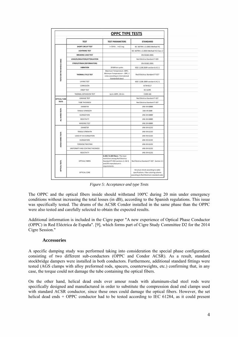
Below some of the acceptance tests and type tests carried out over the OPPC conductor are shown:

TEST TEST PARAMETERS STANDARD

TENSILE STRENGTH TEST EN 50182:2001

LOAD/ELONGATION/ATTENUATION Red Eléctrica Standard IT‐029

LEAKAGE TEST/TIGHTNESS TEST Red Eléctrica Standard IT‐027

TUBE THICKNESS Red Eléctrica Standard IT‐027

OPPC FACTORY ACCEPTANCE TESTS

TEST

S FO

R

THE W

HOLE

CABLE

OPTICAL TUBE

TESTS

4

Figure 5: Acceptance and type Tests

The OPPC and the optical fibers inside should withstand 100ºC during 20 min under emergency conditions without increasing the total losses (in dB), according to the Spanish regulations. This issue was specifically tested. The drums of the ACSR Condor installed in the same phase than the OPPC were also tested and carefully selected to obtain the expected results. Additional information is included in the Cigre paper "A new experience of Optical Phase Conductor (OPPC) in Red Eléctrica de España". [9], which forms part of Cigre Study Committee D2 for the 2014 Cigre Session." Accessories A specific damping study was performed taking into consideration the special phase configuration, consisting of two different sub-conductors (OPPC and Condor ACSR). As a result, standard stockbridge dampers were installed in both conductors. Furthermore, additional standard fittings were tested (AGS clamps with alloy preformed rods, spacers, counterweights, etc.) confirming that, in any case, the torque could not damage the tube containing the optical fibers. On the other hand, helical dead ends over amour roads with aluminum-clad steel rods were specifically designed and manufactured in order to substitute the compression dead end clamps used with standard ACSR conductor, since these ones could damage the optical fibers. However, the set helical dead ends + OPPC conductor had to be tested according to IEC 61284, as it could present

TEST TEST PARAMETERS STANDARD

SHORT CIRCUIT TEST I= 50 KA ; t=0,5 seg IEC 60794‐1‐2:2003 Method H1

LIGHTNING TEST IEC 60794‐1‐2:2003 Method H2 Class 2

BREAKING LOAD TEST EN 50182:2001

LOAD/ELONGATION/ATTENUATION Red Eléctrica Standard IT‐029

STRESS/STRAIN (DEFORMATION) EN 50182:2001

VIBRATION 20 Million cycles IEEE 1138:2009 section 6.4.3.1

THERMAL CYCLE TEST

Maximum Temperature =90ºC;

Minimum Temperature= ‐ 20ºC; 2

ciclos according to International

Standards(6 days)

Red Eléctrica Standard IT‐027

LAYING TEST IEEE 1138‐2009 section 6.4.2.1

CORROSIÓN ASTM B117

CREEP TEST IEC 61395

THERMAL EXPANSION TEST Up to 100ºC, 30 min CIGRE 426

LEAKAGE TEST Red Eléctrica Standard IT‐027

TUBE THICKNESS Red Eléctrica Standard IT‐027

DIAMETER UNE‐EN 60889

TENSILE STRENGTH UNE‐EN 6089

ELONGATION UNE‐EN 60889

RESISTIVITY UNE‐EN 60889

WINDING TEST UNE‐EN 60889

DIAMETER UNE‐EN 61232

TENSILE STRENHTH UNE‐EN 61232

LOAD AT 1% ELONGATION UNE‐EN 61232

ELONGATION UNE‐EN 61232

TORSION/TWISTING UNE‐EN 61232

UNIFORMITY AND COATING THICKNESS UNE‐EN 61232

RESISTIVITY UNE‐EN 61232

OPTICAL FIBRES

G.652 / G.655 fibers: The most

restrictive among Red Eléctrica

Standard ET‐032 (sections 3, 4 & 5)

and DTS manufacturer's

requirements.

Red Eléctrica Standard IT‐027 ‐ Section 2.1

OPTICAL CORE

Structure check according to cable

specifications. Fiber coloring scheme

according to Red Eléctrica's standard code.

OPTICAL TESTS

OPPC TYPE TESTS

OPTICAL TUBE

TESTS

AL1 W

IRES TESTS

A20SA

WIRES TESTS

TESTS FO

R THE WHOLE CABLE

5

problems to withstand the efforts transmitted from the outer layers to the steel core if they have an inappropriate design or insufficient length to spread the load properly. Moreover, temporary helical dead ends (shorter than the final helical dead ends) were designed in order to handle the OPPC conductor during the laying and stringing processes. Additional tests were required in order to define the effect of the temporary helical dead ends and the self-griping clamps (normally used during the laying process) over the tube containing the optical fibers.

Figure 6: Helical dead-end arrangement and self-griping clamps.

The optical attenuation was continuously monitored during tests, and the ovality of the OF tube was measured in portion of non tested conductors and in conductors where the temporary tension devices had been installed.

The ovality of the OF tube measured in a non tested conductor was 0,5%, the ovality of the OF tube in a portion of conductor located under the helical dead end was 0,68% and finally, the ovality of the tube under self-gripping clamps was 5,5%. However, in the last case some spots with higher ovality were detected (13,7%). As a result of these tests, it was decided to use temporary helical dead ends, except in case of low load conditions in which self-gripping clams could be accepted.

Figure 6.1: Tensile cycling test results

6

Termination units Termination Units (TU) were installed at both ends of the OPPC in order to split up the power conductor from the optical fibers. These devices are located inside the Maria and Fuendetodos substations. The fibers bundle integrated in the 220 kV isolator of the TU are terminated and spliced in splicing cassettes at the top and bottom housing of the accessory. In Fuendetodos, the Optical fibers end at the TU, but in Maria these optical fibers were spliced with an isolated optical conductor which continues up towards the close building where the Monitoring system is located.

Figure 7: Termination Unit

Straight joints Compression mid-span joints cannot be used with this kind of conductors due to the need of splicing optical fibers. Hence, in this project the joints were installed in the jumper of several tension towers distributed along the route of the line. This constraint required customizing the conductor length of every drum according to their maximum allowable weight and dimensions. The straight joints should be installed in those anchoring towers where there was enough space for the brake machine or the pulling winch. Apart from that, a scissor lift is necessary to handle the joint for the Optical fiber team. Consequently, this space must be taken into account in order to calculate the temporary occupation during the construction stage.

Figure 8. Straight joints.

Especial suspension fittings were designed to install the straight joint in the jumper. One of the specific issues of this project was to keep in balance the suspension fittings, due to the fact that the lower phase consists of a particular twin bundle configuration (Condor ACSR and OPPC conductor). There are big differences between the weight of the straight joints and the weight of suspension clamps (GS Grip Suspension). This asymmetrical configuration had to be carefully designed and arranged to avoid sag differences within the two types of conductors. Also, the OPPC straight-joint

7

closure has connected an additional conductor jumper in order to avoid interrupting the flow of the electrical current if any damage happens in the joint.

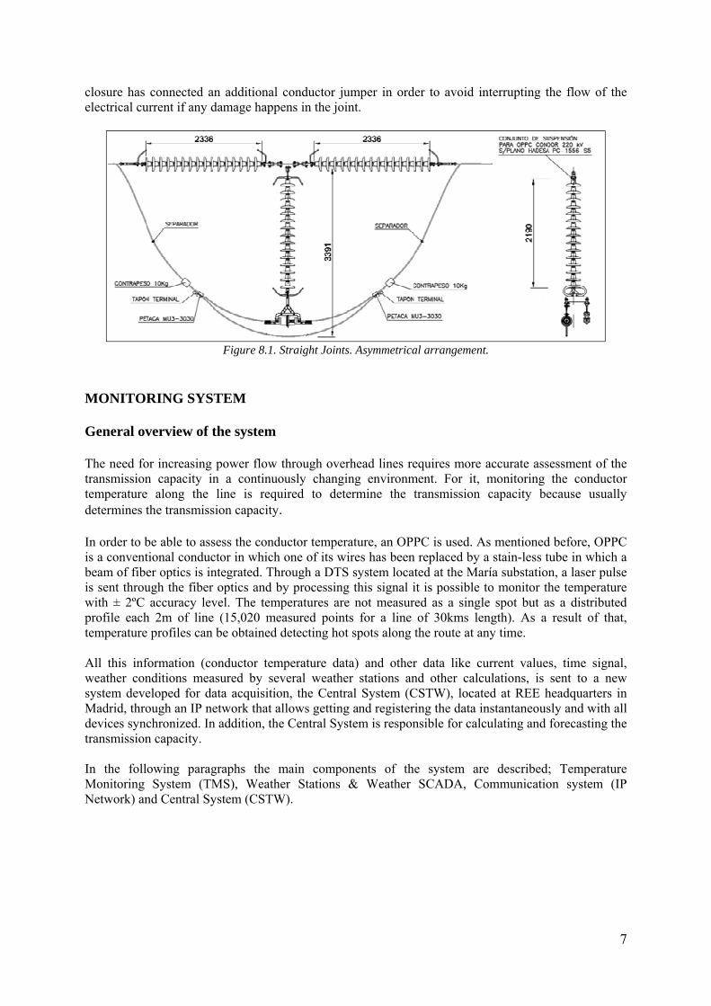
Figure 8.1. Straight Joints. Asymmetrical arrangement.

MONITORING SYSTEM General overview of the system The need for increasing power flow through overhead lines requires more accurate assessment of the transmission capacity in a continuously changing environment. For it, monitoring the conductor temperature along the line is required to determine the transmission capacity because usually determines the transmission capacity. In order to be able to assess the conductor temperature, an OPPC is used. As mentioned before, OPPC is a conventional conductor in which one of its wires has been replaced by a stain-less tube in which a beam of fiber optics is integrated. Through a DTS system located at the María substation, a laser pulse is sent through the fiber optics and by processing this signal it is possible to monitor the temperature with ± 2ºC accuracy level. The temperatures are not measured as a single spot but as a distributed profile each 2m of line (15,020 measured points for a line of 30kms length). As a result of that, temperature profiles can be obtained detecting hot spots along the route at any time. All this information (conductor temperature data) and other data like current values, time signal, weather conditions measured by several weather stations and other calculations, is sent to a new system developed for data acquisition, the Central System (CSTW), located at REE headquarters in Madrid, through an IP network that allows getting and registering the data instantaneously and with all devices synchronized. In addition, the Central System is responsible for calculating and forecasting the transmission capacity. In the following paragraphs the main components of the system are described; Temperature Monitoring System (TMS), Weather Stations & Weather SCADA, Communication system (IP Network) and Central System (CSTW).

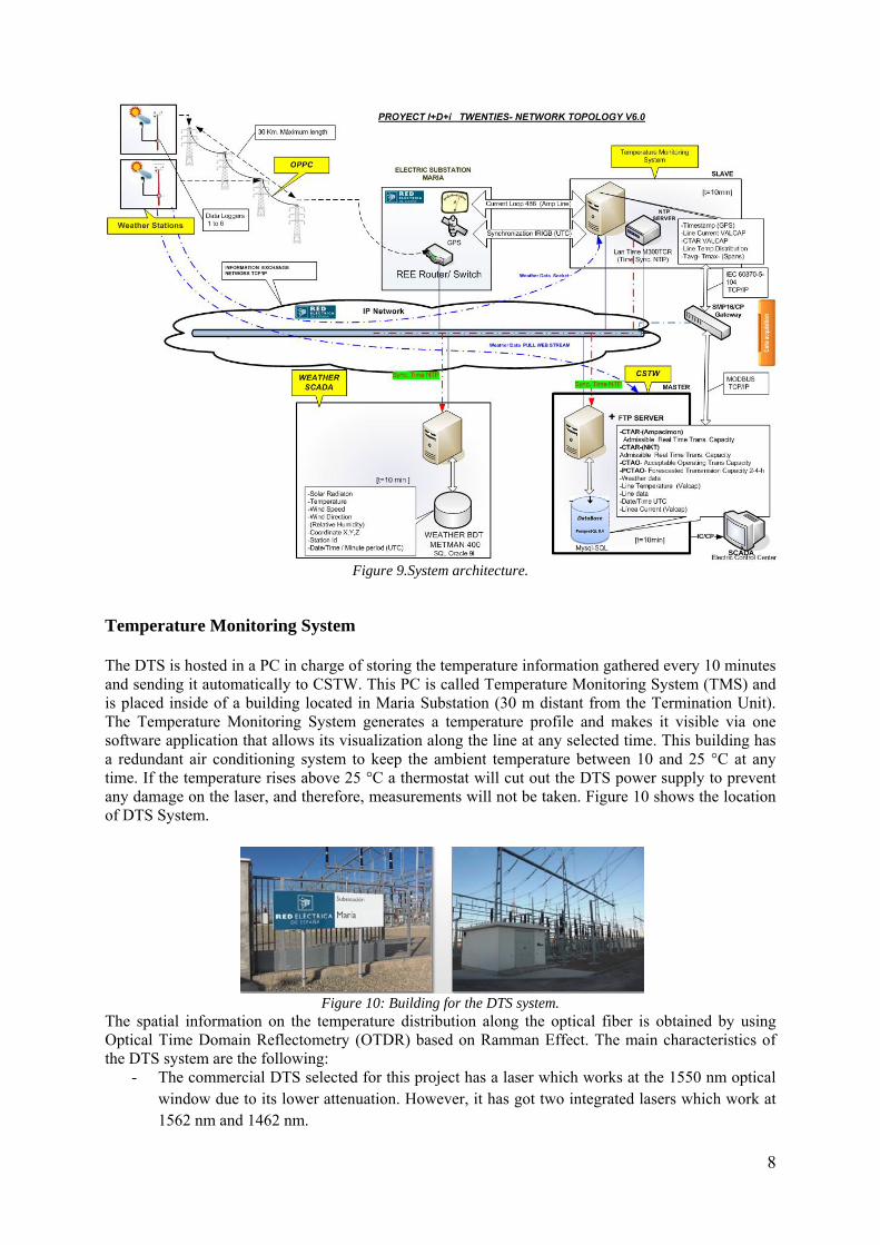
8

Figure 9.System architecture.

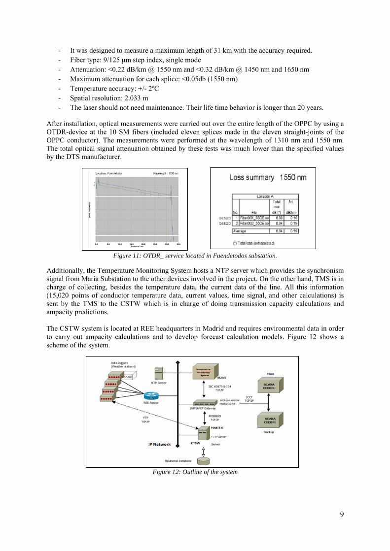
Temperature Monitoring System The DTS is hosted in a PC in charge of storing the temperature information gathered every 10 minutes and sending it automatically to CSTW. This PC is called Temperature Monitoring System (TMS) and is placed inside of a building located in Maria Substation (30 m distant from the Termination Unit). The Temperature Monitoring System generates a temperature profile and makes it visible via one software application that allows its visualization along the line at any selected time. This building has a redundant air conditioning system to keep the ambient temperature between 10 and 25 °C at any time. If the temperature rises above 25 °C a thermostat will cut out the DTS power supply to prevent any damage on the laser, and therefore, measurements will not be taken. Figure 10 shows the location of DTS System.

Figure 10: Building for the DTS system.

The spatial information on the temperature distribution along the optical fiber is obtained by using Optical Time Domain Reflectometry (OTDR) based on Ramman Effect. The main characteristics of the DTS system are the following:

- The commercial DTS selected for this project has a laser which works at the 1550 nm optical window due to its lower attenuation. However, it has got two integrated lasers which work at 1562 nm and 1462 nm.

9

- It was designed to measure a maximum length of 31 km with the accuracy required. - Fiber type: 9/125 μm step index, single mode - Attenuation: <0.22 dB/km @ 1550 nm and <0.32 dB/km @ 1450 nm and 1650 nm - Maximum attenuation for each splice: <0.05db (1550 nm) - Temperature accuracy: +/- 2ºC - Spatial resolution: 2.033 m - The laser should not need maintenance. Their life time behavior is longer than 20 years.

After installation, optical measurements were carried out over the entire length of the OPPC by using a OTDR-device at the 10 SM fibers (included eleven splices made in the eleven straight-joints of the OPPC conductor). The measurements were performed at the wavelength of 1310 nm and 1550 nm. The total optical signal attenuation obtained by these tests was much lower than the specified values by the DTS manufacturer.

Figure 11: OTDR_ service located in Fuendetodos substation.

Additionally, the Temperature Monitoring System hosts a NTP server which provides the synchronism signal from Maria Substation to the other devices involved in the project. On the other hand, TMS is in charge of collecting, besides the temperature data, the current data of the line. All this information (15,020 points of conductor temperature data, current values, time signal, and other calculations) is sent by the TMS to the CSTW which is in charge of doing transmission capacity calculations and ampacity predictions. The CSTW system is located at REE headquarters in Madrid and requires environmental data in order to carry out ampacity calculations and to develop forecast calculation models. Figure 12 shows a scheme of the system.

Figure 12: Outline of the system

10

Weather Stations The weather stations are installed in 6 tension towers distributed along the line and located 10 meters over the ground, according to the minimum conductor clearance in this project. Furthermore, considering the safety criteria set by the weather station manufacturer regarding electromagnetic field compatibility, the distance between power conductors and sensors should be more than 5 meters. Each weather station consists of: 1. Two Solar Panels (65 W in total, 12V), 30º inclined 2. Batteries (2 x 52 Ah) 3. Multi-sensor: No moving parts.

a. Anemometer: Measurement system is ultrasonic. More reliability close to a HV conductor. Range: 0-60m/s; Wind module accuracy: ±0,1 m/s; Wind direction accuracy ±3º.

b. Ambient temperature. Accuracy ±0,3ºC c. Rain Gauge d. Barometric pressure sensor

4. Radiation sensor 5. Charge Controller: Its priority is feeding the communication system and then feed the batteries.

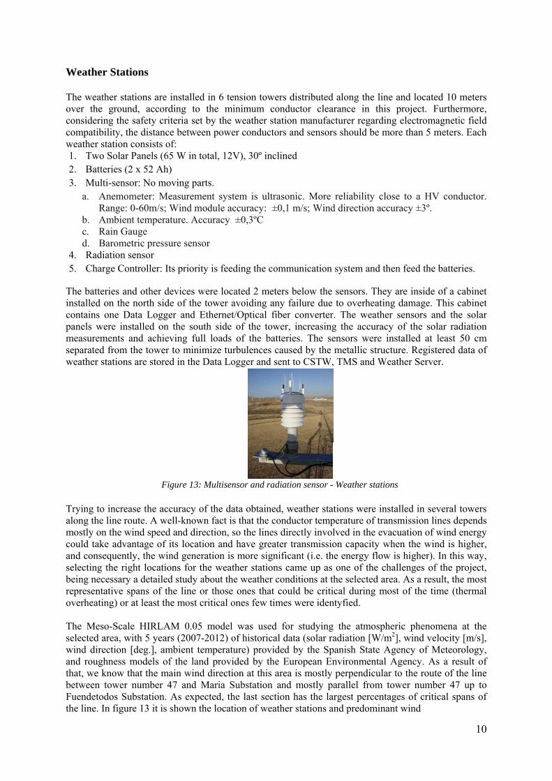
The batteries and other devices were located 2 meters below the sensors. They are inside of a cabinet installed on the north side of the tower avoiding any failure due to overheating damage. This cabinet contains one Data Logger and Ethernet/Optical fiber converter. The weather sensors and the solar panels were installed on the south side of the tower, increasing the accuracy of the solar radiation measurements and achieving full loads of the batteries. The sensors were installed at least 50 cm separated from the tower to minimize turbulences caused by the metallic structure. Registered data of weather stations are stored in the Data Logger and sent to CSTW, TMS and Weather Server.

Figure 13: Multisensor and radiation sensor - Weather stations

Trying to increase the accuracy of the data obtained, weather stations were installed in several towers along the line route. A well-known fact is that the conductor temperature of transmission lines depends mostly on the wind speed and direction, so the lines directly involved in the evacuation of wind energy could take advantage of its location and have greater transmission capacity when the wind is higher, and consequently, the wind generation is more significant (i.e. the energy flow is higher). In this way, selecting the right locations for the weather stations came up as one of the challenges of the project, being necessary a detailed study about the weather conditions at the selected area. As a result, the most representative spans of the line or those ones that could be critical during most of the time (thermal overheating) or at least the most critical ones few times were identyfied. The Meso-Scale HIRLAM 0.05 model was used for studying the atmospheric phenomena at the selected area, with 5 years (2007-2012) of historical data (solar radiation [W/m2], wind velocity [m/s], wind direction [deg.], ambient temperature) provided by the Spanish State Agency of Meteorology, and roughness models of the land provided by the European Environmental Agency. As a result of that, we know that the main wind direction at this area is mostly perpendicular to the route of the line between tower number 47 and Maria Substation and mostly parallel from tower number 47 up to Fuendetodos Substation. As expected, the last section has the largest percentages of critical spans of the line. In figure 13 it is shown the location of weather stations and predominant wind

11

Figure 14: Location of weather stations and predominant wind.

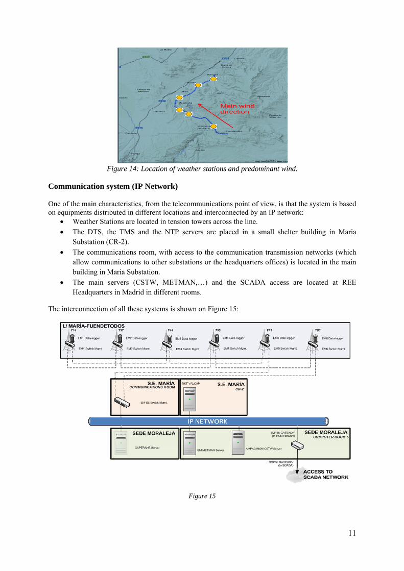
Communication system (IP Network) One of the main characteristics, from the telecommunications point of view, is that the system is based on equipments distributed in different locations and interconnected by an IP network:

Weather Stations are located in tension towers across the line.

The DTS, the TMS and the NTP servers are placed in a small shelter building in Maria Substation (CR-2).

The communications room, with access to the communication transmission networks (which allow communications to other substations or the headquarters offices) is located in the main building in Maria Substation.

The main servers (CSTW, METMAN,…) and the SCADA access are located at REE Headquarters in Madrid in different rooms.

The interconnection of all these systems is shown on Figure 15:

Figure 15

12

The connectivity of the weather stations is particularly significant. IP access in towers has been possible by connecting each weather station to a switch. These switches are optically interconnected with a ring topology using the fiber optics of the OPGW (OPtical Ground Wire) cable installed in the line. This optical ring is also connected to the Communications Room in Maria Substation, enabling the communications with the rest of the equipments of the system. The weather stations data is transmitted every 5 minutes through these optical fibers.

Figure 15.1. Connection of weather stations to OPGW. However, one of the main constraints is the power consumption of the communication elements in the towers. The energy consumption of the weather stations due to this communication through the optical fibers is 725 mAh (700 mAh only for the communication system) or 209 Wh per day. So, the right dimensioning of this feeding system is crucial for the project. Central System Weather information is needed to adjust the forecasted ampacity models implemented in the CSTW. The CSTW server receives weather data, current values and temperature profiles every 5 or 10 minutes depending on the data. The algorithms are executed every 5 minutes and the results are stored in a database. The purpose of this CSTW is:

First of all, storing the information about the line’s temperature and the weather stations (like a backup).

Secondly, perform the calculations generated by the algorithms to obtain the following values: ‐ CTAR Compute Line Ampacity: CTAR is the result of the real time temperature

calculation of the line. It is used as a base value for the calculation of the CTAO and PCTAO outputs and as a comparison value to evaluate the quality of the forecast data. The measured conductor temperature is given by the Temperature Monitoring System (downstream to de DTS). Based on this, the mean conductor temperature is determined for every section of the line. For each section, this temperature is also calculated using the conductor thermal model [2,3] the current and the environmental conditions as input values. The conductor temperature calculated using the environmental parameters (wind speed, wind direction, ambient temperature and solar radiation) measured at a weather station close to the section will always differ from the measured conductor temperature given by the Temperature Monitoring System. This is due to the fact the ambient parameters are not constant along the whole section producing axial differences in the conductor [5, 6]. Therefore, the CTW System adapts the ambient conditions by comparing the measured mean conductor temperature with the calculated mean conductor temperature. The resulting weather values are called effective values.

13

Figure 16. Calculation scheme

‐ CTAO Compute Operational Ampacity: The algorithm is able to compute an operational ampacity which will remain stable and valid for 30 minutes period. This value is used to give the operators a constant figure rather than a moving value and is based on PCTAO calculations for the next 30 minutes.

‐ PCTAO Compute forecast: The algorithm compute a forecast value for the next 30

minutes, 1 hour, 2 hours and 4 hours. Historical data is used to predict the ampacity of the line for a given forecast window. CTSW needs at least 10 days of historical data to be able to compute a forecasted ampacity. This short-term ampacity forecast is currently under-develop.

Figure 17. Calculation results

Control Center: Real Time Operation The Control Center SCADA is connected to the CSTW system, in order to facilitate the Operator decision making. For Real Time operation it is necessary to show via SCADA three significant variables calculated by the CSTW:

- CTAO (MVA) for the last execution (this value is calculated every 5 minutes) - Maximum mean Temperature (ºC) of the critical span - PCTAO (MVA): PCTAO for 1 hour, 2 hours and 4 hours

Also, to have all the information available in the SCADA display it is necessary to show the seasonal ratio and the actual power (MW) transmitted by the monitored line.

14

Figure 18. SCADA Display for Real Time Operation

This way, analyzing the graphic for the CTAO value in the last six hours (graphic available in the SCADA system), the operator can know if the RTTR system is working properly or not. In case the line MARIA-FUENDETODOS were closed to be overcharged according to the seasonal ratio, the operator can know if the line is at risk looking at the temperature in the critical span and also can determine which is the operational margin given by the CTAO (according to data project, the maximum temperature admissible for line MARÍA-FUENDETODOS is 85 º C). Finally, if the operator decided to operate the line according to the RTTR, it is necessary for him to know the PCTAO value for the next hours (1, 2 or 4). With this information, the operator can prepare a scenario to study if the PCTAO will be enough in the next hours or will be necessary to constraint at real time the local wind power generation close to MARIA-FUENDETODOS line. ANALYSIS OF PRELIMINARY RESULTS The results obtained using the model and algorithms developed are being analyzed (on-going). An initial study of the data and measurements of a three-month period, from April 1 to June 30, 2013 has been carried out and it is shown in the following sections. Temperature variation

With the aim of showing the temperature profile and its daily variation, one day has been selected, as an example, to perform the analysis of the temperature evolution. Three moments has been chosen (3:00, 11:00 and 19:00). In the analysis, the conductor temperature profile has been spliced into several sections (length of the line between tension towers). Section 1-2 is the closest ones to Fuendetodos substation, and section 85-86 is the closest ones to Maria substation. Temperature steps between sections have been observed in the graphs below. This demonstrates the wind direction effect over the transmission capacity, checking that the direction changes of several sections along the route regarding to the wind direction determine the variability of the conductor temperature. May 15 at 3:00, 11:00 and 19:00

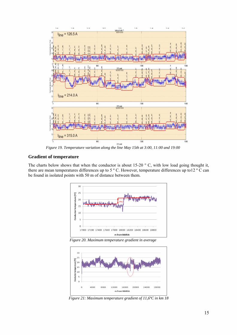
15

Figure 19. Temperature variation along the line May 15th at 3:00, 11:00 and 19:00

Gradient of temperature

The charts below shows that when the conductor is about 15-20 ° C, with low load going thought it, there are mean temperatures differences up to 5 º C. However, temperature differences up to12 º C can be found in isolated points with 50 m of distance between them.

Figure 20. Maximum temperature gradient in average

Figure 21: Maximum temperature gradient of 11,6ºC in km 18

16

According to the results, when load increases and the line works at temperatures far from the ambient ones, higher punctual differences could be found. Therefore, considering the secure operation of the line, taking into account a single conductor temperature measurement should not be enough in order to apply RTTR models to the real time operation. This is one of the reasons why a DTS-TMS has been installed in this line to continuous monitoring of the temperature instead of monitoring the conductor temperature in discrete points of the line. Probability distribution of critical sections location

The graph below represents probability distributions about the most critical sections during the 3 months studied.

Figure 22. Hot sections vs. line km between March and June 2013

The table below provides important information about those sections with the largest critical percentages (sections that have been critical more times) in order to reinforce the idea that the most critical sections are the closest ones to Fuendetodos substation, as it was concluded previously. These critical sections of the line determines its maximum ampacity.

Section25 (77-80)

Section26 (80-83)

Section27 (83-84)

Section28 (84-85))

Section29 MARÍA (85-86)

1% 1% 1% 1% 4% Section17

(52-55) Section18

(55-61) Section19

(61-62) Section20

(62-63) Section21

(63-66) Section22

(66-70) Section23

(70-71) Section24

(71-77)

1% 1% 1% 1% 0% 0% 1% 1% Section9 (26-27)

Section10 (27-28)

Section11 (28-33)

Section12 (33-37)

Section13 (37-44)

Section14(44-47)

Section15 (47-51)

Section16 (51-52))

1% 2% 5% 11% 3% 1% 0% 0% Section1

FUENDETODOS (1-2)

Section2 (2-6)

Section3 (6-8)

Section4 (8-14)

Section5 (14-22)

Section6 (22-24)

Section7 (24-25)

Section8 (25-26)

11% 12% 18% 5% 10% 5% 1% 1%

Table 23. Critical section location

According to these conclusions, it could be possible to say that WS A is not necessary. However, the areas E and F are critical due to the wind direction variability. Finally, B and C areas show a great variability in their measurements making not possible to forecast when these areas could be the most critical ones. Thus, it should be mandatory to monitor their changing weather conditions. Remind that the location of the weather station is the result of a developed study about weather conditions in order to obtain the most representative spans of the line or at least those ones that could be critical most of the time. A, B and C were located in the most favorable stretch of the line in order to find representative points of the line, not only the most critical. Thus, the development of these previous meteorological studies should be considered in RTTR projects. Indeed, should be very interesting

17

developing these studies in previous steps of the project, before defining the route of the line, in order to taking into account this information as an additional parameter for the design stage. Otherwise, during the period of study (3 months) all the sections have been critical except sections 21 and 22. Analysis of the critical sections location The critical section is explained in terms of the highest mean temperature of the critical section. Thus, the parameters with influence in the transmission capacity should be analyzed in order to determine the factor with highest weight. Four factors have been considered: 1.- Wind speed, 2.- Air temperature, 3.- Angle between wind direction and the route of the line and 4.- Solar radiation. The results for the analyzed factors are given in Table 24.

WSA WSB WSC WSE WSF

Wind Speed (m/s) 3.7 3.5 4.9 4.1 4.3

Standard deviation (m/s) 2.6 2.3 3.6 2.9 2.9

Ambient temperature (ºC) 14.0 14.0 13.8 13.5 11.4

Standard deviation (ºC) 5.1 5.3 5.1 4.9 3.7

Solar Radiation (W/m2) 399 428 397 421 405

Standard deviation (W/m2) 320 328 316 328 317

Max. Solar Radiation (W/m2)

868 931 753 894 918

Standard deviation (W/m2) 217 231 241 222 271 Table 24. Statistics of measured meteorological data

Wind speed. The statistics mentioned above indicates that the less favorable wind speed exists in Weather Station B (WSB). On the other hand, the next figure analyses the percentage in which each weather station registers the less favorable (the most critical) wind speed value for the overhead line cooling. The results are the following:

Figure 25. Percentage of times that every weather station register the most critical wind speed

In conclusion the spans and sections located near to Maria PowerStation (WSA and WSB) usually withstand less wind speed values than the closest ones to Fuendetodos.

Ambient temperature: These figures show that the highest mean ambient temperature (the most critical) is registered in WS A and WS B, near Maria PowerStation.

18

Figure 26. Percentage of times weather stations register the most critical ambient temperature

Angle between wind direction and the route of the line: The following map indicates the wind rose of each weather station (blue arrow) with relation to the direction of the route of the line in that area. Also the most parallel directions (wind direction vs route of the line) are observed in WSE and WSF, near Fuendetodos substation. This matches with the stretch of the line with higher measured conductor temperatures by the TMS. Therefore, the most critical situation for the line cooling exists near Fuendetodos because the wind blows quite parallel to the line route, instead of being the area with the lowest ambient temperature and low wind speed values.

Solar radiation: According solar radiation, there are not big differences along the route of the line. In addition, taking into account ”the conductor thermal model”, the weight of solar radiation in the ampacity calculations has low importance.

In conclusion, the most critical sections are those ones located near Fuendetodos Substation where the most relevant factor that could explain on this situation is the incidence angle of the wind over the line (effective wind values). Hence, a very strong dependence of the conductor temperature with the wind direction was observed. In any case, the local wind variability in this area and the directionality

19

observed on this line (changes of direction between sections) could determine the ampacity of the line mainly under the effect of relatively high speed winds.

On the other hand, a comparison between the meteorological data required for calculating the seasonal operating ratios of a line in Zaragoza and the real values obtained from the WS located in Maria-Fuendetodos line can be checked in the table below. In order to compare these values, considering that ambient temperature of real data is the average of daily temperature average, solar radiation is the average of peaks of each day in the period studied and minimum perpendicular wind (effective wind) is obtained from wind speed and direction values corrected according to the “conductor thermal model” [2,3]. All the collected data obtained from the available weather stations located in the line has been taken into account:

Ambient temperature

(ºC) Solar radiation

(W/m2) Perpendicular Wind

(m/s)

Zaragoza Estándar (Seasonal rating)

31 438 0.60

Real data María - Fuendetodos

12 876 0.73

Table 27. Statistics of meteorological data measured during spring and summer

The comparison conclusion is that the calculation of the static ratio with real data could represent an additional transmission capacity respect the seasonal rating.

Dynamic rate behavior Taking into account the data obtained between April and June, using dynamic ratios could integrate approximately 213.000 MVAh of additional energy. This represents an increase of 15% from the energy transmitted in the static situation as can be checked in the graphs below. Remark that it is avoided one week of missing data because of a system failure.

Figure 28. Instantaneous CTAR April-June

Figure29. Probability distribution of % additional capacity compared to static rate

20

The calculations done show that the maximum CTAR achieved is +168% higher than the seasonal ratio and the minimum CTAR is 27% lower than the seasonal rate (rarer situation with approximately 0 m/s of wind speed and high ambient temperature and solar radiation). Wind power correlation analysis

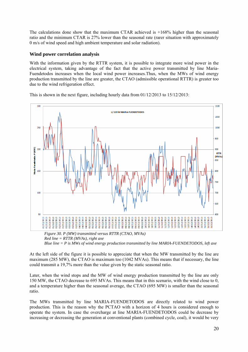
With the information given by the RTTR system, it is possible to integrate more wind power in the electrical system, taking advantage of the fact that the active power transmitted by line Maria-Fuendetodos increases when the local wind power increases.Thus, when the MWs of wind energy production transmitted by the line are greater, the CTAO (admissible operational RTTR) is greater too due to the wind refrigeration effect. This is shown in the next figure, including hourly data from 01/12/2013 to 15/12/2013:

Figure 30. P (MW) transmitted versus RTTR (CTAO, MVAs) Red line = RTTR (MVAs), right axe Blue line = P is MWs of wind energy production transmitted by line MARIA-FUENDETODOS, left axe

At the left side of the figure it is possible to appreciate that when the MW transmitted by the line are maximum (285 MW), the CTAO is maximum too (1042 MVAs). This means that if necessary, the line could transmit a 19,7% more than the value given by the static seasonal ratio. Later, when the wind stops and the MW of wind energy production transmitted by the line are only 150 MW, the CTAO decrease to 695 MVAs. This means that in this scenario, with the wind close to 0, and a temperature higher than the seasonal average, the CTAO (695 MW) is smaller than the seasonal ratio. The MWs transmitted by line MARIA-FUENDETODOS are directly related to wind power production. This is the reason why the PCTAO with a horizon of 4 hours is considered enough to operate the system. In case the overcharge at line MARIA-FUENDETODOS could be decrease by increasing or decreasing the generation at conventional plants (combined cycle, coal), it would be very

21

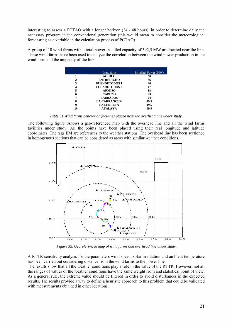
interesting to assess a PCTAO with a longer horizon (24 - 48 hours), in order to determine daily the necessary program in the conventional generation (this would mean to consider the meteorological forecasting as a variable in the calculation process of PCTAO). A group of 10 wind farms with a total power installed capacity of 392,5 MW are located near the line. These wind farms have been used to analyze the correlation between the wind power production in the wind farm and the ampacity of the line.

Wind farm Installed Power (MW) 1 AGUILO 50 2 ENTREDICHO 36 3 FUENDETODOS 1 46 4 FUENDETODOS 2 47 5 ARMIJO 18 6 CABEZO 23 7 LABRADOS 24 8 LA CARRANCHA 49.5 9 LA SERRETA 49.5 10 ATALAYA 49.5

Table 31.Wind farms generation facilities placed near the overhead line under study.

The following figure 0shows a geo-referenced map with the overhead line and all the wind farms facilities under study. All the points have been placed using their real longitude and latitude coordinates. The tags EM are references to the weather stations. The overhead line has been sectioned in homogenous sections that can be considered as areas with similar weather conditions.

Figure 32. Georeferenced map of wind farms and overhead line under study.

A RTTR sensitivity analysis for the parameters wind speed, solar irradiation and ambient temperature has been carried out considering distance from the wind farms to the power line. The results show that all the weather conditions play a role in the value of the RTTR. However, not all the ranges of values of the weather conditions have the same weight from and statistical point of view. As a general rule, the extreme value should be filtered in order to avoid disturbances in the expected results. The results provide a way to define a heuristic approach to this problem that could be validated with measurements obtained in other locations.

22

Effective Wind speed [m/s]

Distance [km] 0‐3 3‐6 6‐9 >9

All RTTR = 0.771 P + 789.3 RTTR = 0.548 P+ 840.9 RTTR = 0.332 P + 943.5 RTTR = ‐0.143 P + 1152.3

d < 10 RTTR = 1.695 P + 783.6 RTTR = 1.269 P + 832.9 RTTR = 0.927 P + 913.8 RTTR = 0.944 P + 956.2

10 < d < 20 RTTR = 6.614 P + 798.6 RTTR = 4.594 P + 859.0 RTTR = 1.305 P + 1003.9 RTTR = ‐3.252 P + 1200.5

20 < d < 30 RTTR = 4.409 P + 802.5 RTTR = 2.667 P + 866.7 RTTR = 0.794 P + 1003.4 RTTR = ‐1.586 P + 1188.0

d > 30 RTTR = 1.661 P + 808.6 RTTR = 1.448 P + 861.9 RTTR = 0.708 P + 983.1 RTTR = ‐0.710 P + 1164.9

Figure 33. Linear Correlation RTTR [MVA] vs P [MW] for distance & effective wind speed.

Figure 34.Linear Correlation RTTR [MVA] vs P [MW] for distance & solar irradiance.

Ambient temperature [ºC]

Distance [km] 0‐10 10‐20 20‐30 >30

All RTTR = 0.548 P + 864.7 RTTR = 0.649 P + 816.5 RTTR = 0.846 P + 724.4 RTTR = 0.247 P + 580.4


10 < d < 20 RTTR = 4.472 P + 887.6 RTTR = 5.908 P + 825.0 RTTR = 6.977 P + 732.8 RTTR = 1.813 P + 583.5


d > 30 RTTR = 1.618 P + 878.7 RTTR = 1.739 P + 836.6 RTTR = 0.927 P + 745.6 RTTR = 0.569 P + 583.0

Figure 35.Linear Correlation RTTR [MVA] vs P [MW] for distance & ambient temperature.

The following table shows the polynomial equation that confirms the existence of a linear correlation between RTTR of the line and wind farms production, highly affected by the effective wind.

Distance km April-June April May June

Not considered RTTR = 0.7343 P + 800.33 RTTR = 0.6841 P + 840.17 RTTR = 0.7334 P + 814.54 RTTR = 0.6685 P + 743.32 '




30 < d RTTR = 0.7343 P + 800.33 RTTR = 1.8711 P + 860.80 RTTR = 2.2883 P + 830.84 RTTR = 1.8213 P + 754.96

Figure 36.Linear correlation of RTTR [MVA] vs P [MW].

Solar irradiance [W/m^2]

Distance [km] 0‐200 200‐400 400‐600 600‐800 >800

All RTTR = 0.639 P + 806.7 RTTR = 0.787 P + 820.2 RTTR = 0.850 P + 805.0 RTTR = 0.906 P + 785.1 RTTR = 0.949 P + 761.5

d < 10 RTTR = 1.399 P + 803.4 RTTR = 1.765 P + 811.4 RTTR = 1.868 P + 796.6 RTTR = 2.041 P + 773.5 RTTR = 2.149 P + 751.6

10 < d < 20 RTTR = 5.660 P + 819.1 RTTR = 7.040 P + 833.1 RTTR = 7.947 P + 814.3 RTTR = 8.625 P + 792.9 RTTR = 8.948 P+769.68

20 < d < 30 RTTR = 3.472 P + 825.1 RTTR = 4.047 P + 841.9 RTTR = 4.389 P + 825.6 RTTR = 4.750 P + 805.5 RTTR = 5.120 P + 780.2

d > 30 RTTR = 1.848 P + 819.0 RTTR = 2.225 P + 842.2 RTTR = 2.400 P + 832.0 RTTR = 2.409 P + 817.9 RTTR = 2.682 P + 787.9

23

Figure 37.RTTR [MVA] vs P [MW] for all wind farms in April-June 2013 and linear regression.

Conclusions

The technology has passed all the technical validation phases by simulations, lab testing and finally field tests demonstrating that the functionality aimed is successfully achieved. The main results obtained are the following:

Calculation of the CTAO in real time. We have identified that, most of the days, the dynamic line ratio is an average of 15% upper than the seasonal rating. In these days with more wind generation the dynamic ratio could be higher than 100% of the static ones during the day.

Monitoring the temperature of the entire line without estimation and extrapolations. The demo is recording 15.020 points of temperature (each 2 meters) every 10 minutes. The certainty is total. This way is possible to operate the line using Dynamic Thermal Ratings instead of the seasonal ones.

Hot spot detection is being located for maintenance purposes. It permits studying the correlation between wind production and the increase of transmission

capacity in lines affected by the same local weather conditions. The use of OPPC conductors to assess the operating temperature can be a powerful tool to validate the thermal models of overhead lines. It has to be combined with the use of weather stations along the route to validate a proper approach for dynamic ratings and wind assessment. Therefore, a sensible application of this technology would provide extra-capacity for the renewable generation integration, as well as it will allow a more efficient management of the electrical grid with the current level of safety. Acknowledgements

The works and developments required for the elaboration of this paper have been carried out partially within TWENTIES project (www.twenties-project.eu) which belongs to the Seventh Framework Program funded by European Commission It is recognised the work and participation of the following companies in the development of the project: AMPACIMON, NKT cables, SAPREM and University of Cantabria.

24

BIBLIOGRAPHY [1] TWENTIES Project: Transmission system operation with large penetration of Wind and other

renewable Electricity sources in Networks by means of innovative Tools and Integrated Energy Solutions.

[2] IEEE Std. 738, “Standard for Calculating the Current-Temperature Relationship of Bare Overhead Conductors”. New York, 2011.

[3] CIGRE Technical Brochure 207, “Thermal behaviour of overhead conductors”. Paris, August 2002.

[4] M.W. Davis, “A new thermal rating approach: the real-time thermal rating system. Part 2, steady-state thermal rating system”. Transactions IEEE Power Apparatus and Systems, 1977.

[5] D.A. Douglass, B. Clairmont, J. Iglesias, Z. Peter. “Radial and Longitudinal Temperature Gradients in Bare Stranded Conductors with High Current Densities”. Cigré Paper B2-108, Paris, August 2012.

[6] W.A. Chisholm, J.S. Barrett. “Ampacity Studies on 49ºC-Rated Transmission Line”, IEEE Transactions on Power Delivery, April 1989.

[7] CIGRE Technical Brochure 498, “Guide for Application of Direct Real-Time Monitoring Systems”. Paris, June 2012

[8] S. Hoffmann, “The use of weather predictions to enhance overhead line ratings”. Cigre Paper B2-5, Edinburgh, September 2003.

[9] Cigre paper "A new experience of Optical Phase Conductor (OPPC) in Red Eléctrica de España". [9], Committee D2 for the 2014 Cigre Session."

dynamic assessment of overhead line capacity for

Documents