Dynamic Capacity Management with Substitution

Robert A. ShumskySimon School of BusinessUniversity of RochesterRochester, NY 14627

shumsky@simon.rochester.edu

Fuqiang ZhangUC Irvine Graduate School of Management

University of CaliforniaIrvine, CA 92697-3125fzhang@uci.edu

April, 2003. Lastest revision: October, 2004

Abstract

We examine a multiperiod capacity allocation model with upgrading. There are multipleproduct types, corresponding to multiple classes of demand, and the firm purchases inventoryof each product before the first period and thereafter replenishment is not possible. Withineach period, after demand arrives, products are allocated to customers. Customers who arriveto find that their product has been depleted can be upgraded by at most one level. We showthat the optimal solution is a simple two-step algorithm: first use any available inventory tosatisfy same-class demand and then upgrade customers until inventory reaches a protectionlimit. We describe how to find optimal protection limits by backward induction and show thatthe protection limits are monotonic in current inventory and in time. The monotonicity resultslead to simple bounds for the optimal protection limits, and we demonstrate that heuristicprotection limits based on the bounds are effective in solving large problems.For a model with two time-periods and two products (dedicated and flexible), we compare

the optimal initial capacity under our dynamic model with the optimal capacity under a single-period ‘static’ model. For a given capacity level, the marginal value of the dedicated capacity isalways greater under the dynamic model than under the static model. Numerical experimentsshow that the optimal level of dedicated capacity is greater under the dynamic model than underthat static model, although the optimal flexible capacity can be smaller, or greater, under thedynamic model.Keywords: inventory management, dynamic programming, rationing policy, revenue man-

agement.

1 Introduction

Many manufacturing and service firms use capacity (or inventory) flexibility to meet uncertain

demand from multiple classes of customers. When inventory for a particular product has been

exhausted, demand for that product may be met by a substitute product. For many applications

the assignment of inventory to customers is complicated by the fact that demand arrives over time

and inventory must be allocated before demand is fully known. Consider the problem faced by a

1

rental car agency. If the customer’s requested car is unavailable, the agency may choose to upgrade

the customer to a more expensive car. Customers arrive throughout the day, and this allocation

decision must be made when the day’s total demand for the higher-value car is still uncertain.

Similar decisions appear in other services (e.g., hotels allocating rooms, airlines allocating economy

and business-class seats) as well as in manufacturing (e.g., a firm choosing to use a high-value part

when a lower-valued part is sufficient but unavailable).

Here we analyze a dynamic multi-product inventory model in which demand arrives in discrete

intervals. Throughout this paper we use the terms ‘inventory’ and ‘capacity’ interchangeably, for

the products may be interpreted as either service capacities or perishable inventories. We describe

a stylized model of the problem faced by the rental car agency each day: how much inventory

should be acquired before the day begins, and how should that inventory be distributed among

customers as the day evolves? The model has the following attributes:

1. There is a single opportunity to invest in inventory before any demand is realized.

2. The period after the initial investment is broken into a finite number of intervals, and the

decision-maker allocates inventory to customers after observing all demand within each in-

terval. In practice, demand may arrive continuously, but as Topkis (1968) points out, the

assumption that demand arrives in discrete intervals “might be expected to be a good ap-

proximation to reality if the intervals are made ‘small enough.’ ”

3. Demand that is not satisfied in each period is lost (there is no backlogging).

4. Demand for a product can be met by a product from the next-higher class (for example, a

rental agency’s demand for a compact car may be met with a full-size car).

5. Inventory may be rationed, so that the firm may choose not to allocate high-class inventory

to a lower-class customer.

We are most interested in the impact of characteristic (2), the assumption that customers ar-

rive over a sequence of time intervals. As we will see in the following literature review, there exist

numerous articles that examine the benefits of inventory flexibility. However, most authors assume

2

that all demand appears simultaneously, or that if demand appears over time then inventory is

allocated only after the last customer arrives. Given this perfect information about demand, in-

ventory can be allocated optimally. However, for many applications this ‘single-period’ assumption

overestimates profits and, as we shall see, may also overestimate the value of inventory flexibility.

Therefore, this model can be seen as an extension of the single-period multi-product newsven-

dor models of Bassok et al. (1999), Netessine et al. (2002), and others, to an environment with

multi-period demand. Another model with this flavor is the ‘newsvendor network’ of Van Mieghem

and Rudi (2002), but their model allows the firm to replenish inventories between each period. Our

model is also similar to yield management models in which a firm must find optimal rules for ra-

tioning inventory among customer classes. Therefore, this paper can also be seen as a generalization

of the yield management problem to include multiple types of inventory as well as the ability to

upgrade customers to a higher inventory class.

After reviewing the literature, we describe the model in Section 3 and show that the single-

period formulation provides an upper bound on the expected profit of our dynamic model. In

Section 4 we prove that a rationing scheme is the optimal policy among all possible policies and

describe a necessary and sufficient condition for the optimal level of rationing (the number of units

to ration is sometimes called the protection limit). In Section 5 we show that the protection limit

of each inventory class is decreasing as time increases and is decreasing in the inventory level of

any of the available products.1 We also derive bounds on both the size of the problem and the

optimal protection limits. The bounds on the size of the problem are expressed in terms of the

number of products and number of remaining time periods. The bounds on the optimal protection

limits are complementary pairs of lower and upper bounds that grow progressively tighter as the

computational effort to calculate the bounds increases. Section 5 ends with numerical experiments

demonstrating that over a wide range of parameters, the bounds are extremely tight. In fact,

bounds based only upon the inventory level of one adjacent product allow us to estimate protection

levels that are extremely close to optimal, and these bounds can be calculated quite quickly.

In Section 6 we focus on the optimal capacity decision. In particular, we examine the problem

with two products, dedicated inventory and flexible inventory, and two time-periods (we will call1Throughout this paper we use decreasing for nonincreasing and increasing for nondecreasing.

3

this the ‘2x2 model’). We compare the 2x2 model with a single-period model; this comparison is

important, for single-period, static models have often been used to evaluate the benefits of flexible

inventory. We prove that, for any given capacity, the marginal value of the dedicated inventory

is larger in the dynamic model than in the static model. In numerical experiments we find that

the optimal initial level of dedicated inventory is always higher in the dynamic model than in the

single-period model. We also find that the optimal initial level of flexible inventory may be lower,

or higher, in the dynamic model than in the static model. This finding contradicts the intuition

that because flexibility may be used to greater advantage in the static setting than in the dynamic

setting, flexible inventory should always be more valuable - and therefore should be more plentiful

- in the static setting.

2 Related Literature

There are many models in the literature that capture a subset of the five characteristics described

above, but none, to our knowledge, address all five. See Van Mieghem, 2003, for a survey of

models to study capacity investment and management. Some researchers have focused on single-

period multidimensional newsvendor models. For example, Bassok et al. (1999) propose a general

multiproduct inventory model to study the benefits of substitution. Pasternack and Drezner (1991)

find the optimal stocking policy for goods with stochastic demand and substitution in both the ‘up’

and ‘down’ directions. Fine and Freund (1990) and Van Mieghem (1998) study optimal levels of

flexible and dedicated production capacities. Netessine et al. (2002) study the value of single-level

upgrades with an emphasis on the impact of demand correlation on the optimal investment levels.

In all of these papers, the firm purchases inventory before demand is realized and distributes the

inventory to customers after observing all demand.

As in our paper, Van Mieghem and Rudi (2002) present a multidimensional newsvendor model

that also incorporates multiperiod demand. However, their model allows the firm to replenish

inventory between each period. For the service applications we have in mind, adjustments in

inventory occur over a longer time-scale than the within-period rationing and allocation decisions,

so that the firm must find the optimal allocation, given only the inventory it purchases before the

first period. The firm’s inability to replenish inventory between periods also distinguishes our work

4

from the literature on multiperiod inventory models with transshipment, such as Karmarkar (1981),

Robinson (1990), and Archibald et al. (1997).

The literature on yield management does focus on environments in which inventory-sizing (or

capacity) decisions are made and then inventory must be allocated as demand arrives over time.

See McGill and van Ryzin, 1999, for a survey of this literature. The analysis by Brumelle and

McGill (1993) characterizes the optimal rationing policy for an airline seat allocation problem in

which a fixed seat capacity must satisfy demand for multiple fare classes. The following papers

generalize these results by incorporating cancellations and/or overbooking: Bitran and Gilbert

(1996), Subramanian et. al. (1999), and Zhao and Zheng (2001). In all of these papers there

is a single type of resource, a coach seat on a single-leg flight, so that there is no discussion of

‘upgrades.’

There are a few papers in the yield management area that do address the issue of inventory

substitution. Alstrup et al. (1986) study a dynamic overbooking problem with two inventory classes

and two-way substitution. Karaesmen and van Ryzin (2000) examine a more general overbooking

problem with multiple substitutable inventory classes. Both papers formulate a two-stage model:

first a booking stage, and then an allocation stage after all demand is realized. While substitution

is allowed during the second, allocation stage, there is no substitution as demand arrives during

the booking stage. In our model, substitution may occur during each demand period.

Savin et al. (2004) propose a model that is tailor-made for studying the renting or leasing of

capital equipment to multiple customer classes. As in the traditional yield management literature,

their model focuses on a single type of capacity, but they formulate the problem as a queueing

control problem and allow the rental period to be stochastic rather than uniformly fixed. In

contrast, our model focuses on a single day, during which the inventory is depleted. We do not

explicitly consider the differential value of customers who will rent for multiple days. Instead, we

focus on the value of inventory substitution and the impact of sequential arrivals on the optimal

initial capacity.

Researchers have also addressed the topics of substitution and rationing in the context of pro-

duction and inventory control. The model of Topkis (1968) is similar to the problem described in

5

this paper. Topkis also assumes a given initial level of inventory and characterizes the optimal

rationing policy as a set of “critical rationing levels,” although his model assumes a single type of

inventory and multiple demand classes. Topkis shows that, under certain conditions, the critical

rationing levels decline over time (analogous results for our model are derived in Section 5, below).

Articles by Ha (1997a, 1997b, and 2000) consider make-to-stock production systems with several

demand classes. These papers show that the optimal stock rationing policy can be characterized by

a sequence of production limits and storage levels that are monotone in customer class. Research by

de Véricourt et al. (2001, 2002) describes the benefits of optimal stock allocation for make-to-stock

systems and present techniques to calculate optimal parameters for the allocation decision. Frank

et al. (2004) consider an inventory system in which replenishment is possible and stock may be

protected from stochastic demand while it is used to fill higher-priority deterministic demand. All

of these papers consider single-item production systems, while we examine a system with multiple

products.

Kapuscinski and Tayur (2000) study a dynamic capacity reservation problem in a make-to-

order environment, in which demands are classified by their waiting-time sensitivities. Eynan

(1999) examines the benefits of inventory pooling and shows that these benefits are not significantly

reduced by the ”cannibalization” of inventory by low-margin customers, but he does not consider

the benefits of a rationing policy. Again, these papers focus on problems involving a single product

and multiple demand classes, while we consider multiple products and demand classes.

3 The Model

In this section we describe the products offered by the firm, the customer demand classes, the cost

and demand parameters (along with a few assumptions about these parameters), and the firm’s

decision variables. At the end of the first subsection we present the problem formulation, while

in the second subsection we present two related formulations and bounds on the objective function

values based on the related formulations.

6

3.1 Problem Description

Consider a firm that serves n classes of demand by providing n types of products indexed by

j = 1, 2, ..., n. Product quality decreases as index j increases, so that product j can be used to

satisfy a customer of class i as long as j ≤ i. This is often called ‘one-way substitution’ and is a

common practice in many service applications. Products with superior quality are acceptable to

customers who request an inferior product, but not vice versa.

Time periods are indexed by t, and demand arrives in each of the t = 1...T periods, where T is

finite. Demand is independent between periods, although product demands within a period need

not be independent. The realized demand in period t is denoted by dti for product i = 1, 2, ..., n.

The joint cumulative distribution function of a given set of random variables in period t is denoted

F t(S), where S ⊆ {1, 2, ...n}, so the complete joint distribution function in period t is F t(1, 2, ...n).The marginal distribution function for product i is F ti . Let D

t = (dt1, dt2, ..., d

tn) denote all realized

demand in period t (in this paper, capitalized, bold-face characters represent vectors). We assume

that each period’s demand for a particular product is a non-negative integer, so that Dt ∈ Z+n .However, all of the following results hold when demand follows any distribution with non-negative

support.

Before the first demand period the firm pays cj for each unit of product j. When a customer

arrives, she pays pj for a product of type j (we assume that all price and cost parameters do not

change over time). The firm may also pay a usage cost uj when a unit is sold. That is, the firm

pays cj up-front, whether the product is sold or not, while uj is only paid if the product is sold to

a customer. The firm may also pay a penalty cost vi if it cannot provide a product to a customer

of type i. We assume that demand is not backlogged, and inventory not sold after period T has

no salvage value. We also assume that the time horizon is sufficiently short so that there is no

discounting of costs or revenues across time periods.

Let αij be the contribution margin for satisfying a class i customer with product j. We make

the following assumptions:

(A1) aij = pi + vi − uj > 0 if j ≤ i ≤ j + 1; aij < 0 otherwise.

7

(A2) p1 + v1 > p2 + v2 > ... > pn + vn;

(A3) u1 > u2 > ... > un.

Assumption (A1) states that only one-step upgrading is profitable. In practice, the profit margin

accrued from multi-step upgrades is often small, or negative. From a network design perspective,

single-step upgrading can often deliver most of the benefits of more complex substitution schemes.

For example, when quantifying the value of flexible production capacity, Jordan and Graves (1995)

find that a chain of factories, each with a single link to its neighbor (each plant i can produce

products i and i + 1) yields nearly the same sales as a chain of factories with full flexibility (each

plant i can produce all products). Here we analyze a similar chain of flexible inventory, although

in our model product n cannot be used to upgrade a customer who desires product 1, so that we

are missing the last ‘link’ in the chain.

Assumptions (A2) and (A3) state that both the revenue (pj+vj) and the usage cost uj decrease

in index j. That is, products with higher quality have higher revenues and usage costs. These

assumptions have several implications. First, they imply that αjj > αkj for all j and k, so that

the maximum margin for product j is achieved by selling to customers of class j. Second, a class

j customer should be upgraded when product j is in stock because the margin from a ‘horizontal’

sale is larger than the profit margin from any present or future upgrade.

Now we describe the firm’s decision variables. Let Xt = (xt1, xt2, ..., x

tn), X

t ∈ Z+n ,be the vectorof inventories at the beginning of period t, t = 1, 2, ..., T. After demand Dt appears, the firm must

make inventory allocation decisions. Let ytij ∈ Z+ be the quantity of product j allocated to classi demand after demand arrives in period t, and let Y

t= (ytij) be the allocation matrix for period

t. Let ΠDYN(X1) be the profit function for our model. We formulate this problem as a dynamic

program with T+1 steps. In period 0 the firm determines the initial inventoryX1, while in periods

1 through T the firm allocates its inventory to maximize its revenue.

Dynamic Substitution Model (DYN)

Period 0:

MaxX1∈Z+n

ΠDYN (X1) = MaxX1∈Z+n

{Θ1(X1)−Xj

cjx1j} (1)

8

Period t (1 ≤ t ≤ T ):

Θt(Xt) = EDt{MaxYt[Gt(Y

t,Dt) +Θt+1(Xt+1)]}

where Gt(Yt,Dt) =

Xi,j

αijytij −

Xi

υidtiX

j

ytij ≤ dti i = 1, 2, ..., n

Xi

ytij ≤ xtj j = 1, 2, ..., n

xt+1j = xtj −Xi

ytij j = 1, 2, ..., n

ytij ∈ Z+ i, j = 1, 2, ..., n

We also define ΘT+1 , 0 under the assumption that the inventory has no salvage value. The

value of Gt(Yt,Dt) is the profit from the single-period capacity problem with substitution. The

first inequality is period t’s demand constraint, the second inequality is period t’s supply constraint,

and the last equality calculates the inventory available for period t+1 (we will refer to this equality

as the ‘linking constraint’).

Note how this formulation corresponds to the daily problem faced by a rental car agency. First,

the agency must decide on X1, the number of cars that should be available at the beginning of

each day. Each time-period t represents an interval within the day (early morning, mid-morning,

etc.), and there are T intervals. The unit cost cj is the cost of having one automobile available

for one day. This may include depreciation, as well as any costs associated with transporting the

car from another location. The variable cost uj , on the other hand, is the cost of an actual rental

(e.g., wear and tear). The solution to the problem maximizes the expected profits over the entire

day. We make the simplifying assumption that the initial inventory vector X1 is the same on each

day, as would be the case if all cars were returned after one day’s rental. The queueing control

model developed by Savin et al. (2001) relaxes this assumption, although their model focuses on a

single product and does not consider the effects of substitution among inventory levels.

9

3.2 Related models

If we let T = 1, model DYN collapses into the single-period (or static) model studied by Bassok et

al. (1999), Netessine et al. (2002), and others (we will use the acronym STC to refer to this model).

For the sake of comparison, we transform the single-period model into an equivalent model with

T periods, and we assume that demand arrives in each period as it does in the dynamic model.

However, in STC, resources are allocated after all demand is observed. This transformation will

help us to compare the performance of STC and DYN, given the same demand. In the following

formulation let X denote the vector of initial inventories and ΠSTC(X) the profit function.

Single-period Substitution Model (STC):

MaxX∈Z+n

ΠSTC(X) = MaxX∈Z+n

E{D1,D2...,DT }

[Θ(X)−Xj

cjxj ] (2)

where

Θ(X) = MaxY[Xi,j

αijyij −Xi

υiXt

dti]

s.t.Xj

yij ≤Xt

dti i = 1, 2, ..., n

Xi

yij ≤ xj j = 1, 2, ..., n

yij ∈ Z+ i, j = 1, 2, ..., n

We also consider the simplest benchmark model, a model without product substitution. This

is equivalent to n independent newsvendors (NV). As in DYN and STC, we consider demand that

arrives sequentially, over T periods. Given independent newsvendors, however, it does not matter

whether the allocation of inventory occurs as the demand arrives (as in DYN) or after the T th

period (as in STC). In either case, the firm determines the optimal inventory xj according to the

newsvendor fractile and then sells the maximum amount of inventory possible.

Independent Newsvendor Model (NV):

MaxX∈Z+n

ΠNV (X)

= MaxX∈Z+n

Xj

{ E{d1j ,d2j ...,dTj }

"αjj min(xj ,

Xt

dtj)− υj(Xt

dtj)

#− cjxj} (3)

10

Next we compare the profits of the three models from the previous section.

Proposition 1 ΠNV (X) ≤ ΠDYN (X) ≤ ΠSTC(X).

Proof. First we show that ΠNV (X) ≤ ΠDYN(X). NV allocates capacity to demand with-

out substitution. Therefore, any allocation of inventory that is feasible in NV is also feasible in

DYN, while DYN has the additional freedom to substitute products. Therefore, for any demand

realization, DYN’s profit is greater than, or equal to, the profit of NV, and ΠNV (X) ≤ ΠDYN(X).Next we show that ΠDYN (X) ≤ ΠSTC(X). In STC, inventory is allocated to customers after the

firm observes all demand. Therefore, for a given demand realization D1,D2, ...,DT , any allocation

decision available in DYN is also a feasible allocation in STC. In addition, there are allocation

opportunities in STC that are not feasible in DYN. Therefore, for any demand realization STC’s

profit is greater than, or equal to, the profit of DYN, and ΠDYN (X) ≤ ΠSTC(X).

This proposition provides us with upper and lower bounds for the dynamic profit function.

Because ΠDYN(X) ≤ ΠSTC(X) for any initial capacity X, ΠDYN (XDYN ) ≤ ΠSTC(XSTC), whereXDYN and XSTC are the optimal initial capacity vectors. In qualitative terms, STC’s profit

function is an upper bound because in that setting there is no demand uncertainty when making

the allocation decision.

4 The optimal policy: greedy allocation and then rationing

In this section we will show that at any time period t, it is optimal to first satisfy demand from

class i with capacity from class i and then to consider upgrades, where upgrading is limited by some

threshold value. More formally, suppose that inventory Xt = (xt1, xt2, ..., x

tn) is available for sale

in period t. Proposition 2 will show that we maximize Θt(Xt) in DYN by following the following

algorithm (henceforth we will refer to this procedure as the ‘GRA,’ for the ‘Greedy-then-Rationing

Algorithm’).

Step 1 : Let ytii = min(dti, x

ti), i = 1, 2, ..., n. Satisfy as much class i demand with product i as

possible.

11

Step 2: Let Nt be the net inventory after full ‘parallel’ allocation:

Nt =¡N t1, N

t2, ..., N

tn

¢=¡xt1 − dt1, xt2 − dt2, ..., xtn − dtn

¢.

Note that N ti can be positive if there is excess capacity, negative if demand exceeds capacity, or

zero. For k = 1, ..., n − 1, if N tk > 0 and N t

k+1 < 0, then let ytk+1,k = N tk − ep. The quantityep ∈ £max(0, N t

k+1 +Ntk), N

tk

¤is the protection limit.

The rationale behind the GRA is straightforward. The profit margin from a ‘horizontal’ sale

is larger than the profit margin from any present or future upgrade, so that in Step 1 any available

capacity should be used to satisfy demand. To understand Step 2, note that a unit of product k

should be upgraded if the current value of the upgrade, αk+1,k is greater than the value of a unit of

that product in the next period. Because the marginal value of product k declines as the quantity

of product k rises (see Lemma 4, below), a threshold rule is optimal when choosing the number of

units to upgrade. The threshold is the protection limit, and if the inventory of a product falls at

or below the protection limit, the product will not be used to satisfy demand from a lower class.

To demonstrate rigorously that the GRA is an optimal policy, we must first derive a series of

intermediate results about the GRA. First, Lemma 1 states that, after Step 1, the optimization

problem breaks into smaller independent ‘subproblems’:

Lemma 1 Suppose that at time t after completing Step 1 of the GRA, Nti ≤ 0, i = k+1, · · · k+ j,

so that the inventories of these products have been depleted. Then the optimization problem can

be separated into two independent problems: an upper part consisting of products 1 to k+ 1, and a

lower part consisting of products k + j + 1 to n.

Proof. Given that only single-step upgrading is profitable, products with indices 1, 2, ...k will

not be used to satisfy demand by classes k + j + 1, ...n. Therefore, the assignment of products in

one group does not affect the capacity or profits of the other group, and the global optimization

problem is separable into the two subproblems.

In general, after Step 1, the global optimization problem may have been divided into numerous

smaller subproblems, each defined by a series of positive net inventories (e.g., Nti > 0, i = j...k) and

12

a single depleted inventory level for the lowest product (Ntk+1 ≤ 0). Therefore, for each subproblem

created after step 1 of the algorithm, there is only one upgrading and rationing decision to be made:

how much capacity of class k do we use for upgrades of unfilled demand from class k + 1?

The same observation applies at the beginning of time t, before step 1 of the GRA. The

global optimization at the beginning of time t may be broken into smaller independent sub-

problems, with boundaries defined by depleted inventories, xti = 0. To be explicit, define B =

{(ht1, lt1), · · · , (htm, ltm)} as the set of upper and lower limits for the subproblems at time t, i.e.,(hti, l

ti) are the indices of the highest (smallest indexed) and lowest (largest indexed) products in

the ith subproblem, so that hti ≤ lti. Then the profit of the remaining optimization problem at

time t, Θt(Xt) in Equation (1) can be written as the sum of the profits from the subproblems:

Θt(Xt) =Xm

i=1Θti(X

ti) (4)

where each subproblem Θti(Xti) has the same formulation as Θ

t(Xt), although the demand and

capacity indices of each subproblem vary from hti to lti, rather than from 1 to n.

To keep the notation simple, for the remainder of this section we will derive the optimal as-

signment policy for an optimization problem Θt(Xt) with product indices i = 1...n. Because the

subproblems are independent, and because the objective function of the global problem is the sum

of the values of the subproblems, the following results apply to any subproblem as well as to the

global optimization problem.

Now consider an alternate formulation of Θt(Xt) that is equivalent to the formulation in Equa-

tion (1). Let Yt = (Pi yti1, ...,

Pi ytin) be the vector of inventory offered to customers in period t.

The capacity Yt may be less than, or equal to, the available capacity Xt. The jth element of Yt,

denoted by ytj =Pi ytij , is the quantity of product j offered for sale during period t. As defined

above, Yt= (ytij) is the entire allocation matrix for period t.

Θt(Xt) = EDt{ MaxYt∈Z+n ,Xt+1∈Z+nYt+Xt+1=Xt

[Ht(Yt,Dt) +Θt+1(Xt+1)]} (5)

13

where Ht(Yt,Dt) = MaxYt[Xi,j

αijytij −

Xi

υidti]X

j

ytij ≤ dti i = 1, 2, ..., n

Xi

ytij ≤ ytj j = 1, 2, ..., n

ytij ∈ Z+ i, j = 1, 2, ..., n.

In this formulation, the conditions Yt ≥ 0,Xt+1 ≥ 0, and Yt +Xt+1 = Xt ensure that the supply

and linking constraints are satisfied.

Given that inventory Yt is available for sale in period t, and given demand realization Dt,

Ht(Yt,Dt) is a simple transportation problem with a cost structure defined by assumptions (A1) -

(A3). Because the data Yt and Dt are integer, the solution to Ht is integer. Bassok et al. (1999)

point out that the cost structure of Ht corresponds to a Monge sequence (Hoffman, 1963), so that

the following algorithm solves the problem.

Lemma 2 Given Yt and Dt, the following algorithm solves Ht(Yt,Dt):,

(i) ytii = min(dti, y

ti), i = 1...n

(ii) yti+1,i = min³¡dti+1 − yti+1

¢+,¡yti − dti

¢+´, i = 1...n− 1.

This appears to be identical to the GRA: greedy assignment, followed by upgrading. However,

we have not yet determined the optimal offered capacity Yt.

Now let Υt(Xt) be the relaxation of Θt(Xt) on the real numbers: Υt(Xt) is identical to formu-

lation (5) but with , Yt ∈ R+n ,Xt+1 ∈ R+n , and ytij ∈ R+.

Lemma 3 The function Υt(Xt) is concave on Xt ∈ R+n .

Proof. The function ΥT (XT ) is concave inXT because (i) a linear program is jointly concave in

variables that determine the right-hand-side of its constraints and (ii) if f(x, ξ) is a concave function

for all possible ξ, then E[f(x, ξ)] is also concave (see van Slyke and Wets [1966], Proposition 7).

Now assume that Υt+1(Xt+1) is concave inXt+1. Because of fact (i) in the previous paragraph,

Ht(Yt,Dt) is concave in Yt for a given Dt. Therefore, given demand Dt, we maximize the sum

14

of two concave functions, Ht(Yt,Dt) + Θt+1(Xt+1), with the constraint Yt + Xt+1 = Xt. By

theorems 5.3 and 5.4 in Rockafeller (1970) this maximal value is concave in Xt. By fact (ii), above,

the expected value taken over demand Dt, Υt(Xt), is also concave in Xt.

Lemma 3 also implies that the relaxation of ΠDYN (X1) on the real numbers is concave.

We are now ready to show that the GRA is an optimal policy. Using the terminology of Porteus

(1975), the set of admissible policies is defined by the constraints of Ht(Yt,Dt), t = 1...T , and

the GRA defines an admissible structured policy. Because of the capacity constraints, all value

functions Θt(Xt) are finite. In the following Lemma we define a structured value function and

show that the GRA attains the optimal value within each period and that the structured value

function is preserved under optimization. For this Lemma, define ∆tk(Xt) = Θt(Xt+ek)−Θt(Xt),

where ek is the kth unit vector; ∆tk(Xt) is the marginal value of one unit of product k.

Lemma 4 Suppose that Θt+1 has the following properties:

1. The GRA solves Θt+1(X).

2. ∆t+1k (X) ≤ αkk.

3. ∆t+1k (X) is decreasing in xt+1k .

Then properties (1)-(3) hold for Θt.

Proof. We will first show that the GRA attains the optimal value for Θt and then we show

that properties (2) and (3) are preserved under optimization.

1. From Lemma 2, we know that a greedy/upgrade algorithm is optimal for any given Yt and

Dt. To show that step 1 of the GRA is optimal, we must show that all available inventory

in Xt is available for step 1’s parallel assignment: ytii = min(dti, x

ti), i = 1...n. Suppose that

ytii < min(dti, x

ti). By Lemma 2, min(d

ti, y

ti) < min(d

ti, x

ti), so that y

ti < x

ti. Therefore, x

ti− yti

units of product i are not used for parallel assignment but are instead held over to the next

period. If any of these units had been used for a parallel assignment in period t, we would

gain αkk in immediate revenue and lose ∆t+1k ≤ αkk. Therefore, ytii = min(d

ti, y

ti) is also an

optimal solution.

15

To show that step 2 is optimal, we must prove the optimality of the rationing scheme for

product k, the product at the ‘bottom’ of the subproblem. Specifically, after Step 1, Lem-

mas 1 and 2 imply that N t1 > 0,N

t2 > 0, ...N

tk > 0, ... , N

tk+1 < 0. We must determine how

much product k capacity should be used to satisfy the unmet demand for product k + 1. If

p is the protection level for product k, we maximize over p,

A(p) = αk+1,k(Ntk − p) +Θt+1((N t

1, Nt2, ..., p, 0))

with the constraint, max(0, N tk+1+N

tk) ≤ p ≤ N t

k. Because ∆t+1k (Xt+1) is decreasing in xt+1k ,

A(p+1)−A(p) is decreasing in p. Let ep be the unconstrained maximizer of A(p). If ep ≤ Q,then because the marginal value of A(p) is decreasing, we should save as little inventory as

possible and upgrade as much as possible: xt+1k = Q. If 0 ≤ ep ≤ Q then it is optimal to

upgrade N tk − ep and ration ep units of product k: xt+1k = ep. If ep > N t

k it is not optimal to use

any units of product k for upgrades: xt+1k = N tk. This shows that a rationing scheme and the

GRA are optimal.

2. To show that property 2 is conserved under optimization, suppose that we begin time period

t with capacity vector X. Consider the following cases: (i) N tk < 0. If the initial capacity

vector had been X + ek, the GRA algorithm would use the additional unit of product k for

parallel assignment, and ∆tk(X) = αkk. (ii) N tk ≥ 0,N t

k+1 ≥ 0. Any extra unit of product kis passed along to the next period, and ∆tk(X) = ∆

t+1k (X) ≤ αkk. (iii) N t

k ≥ 0, N tk+1 < 0. By

the GRA algorithm, if N tk + 1 ≥ ep, the extra unit of product k is used for an upgrade, and

∆tk(X) = αk+1,k < αkk. If N tk +1 < p, the extra unit is passed along to the next period and

∆tk(X) = ∆t+1k (X) ≤ αkk.

3. The optimization problem Θt(Xt) is equivalent to Υt(Xt) when evaluated with integer data.

Lemma 3 indicates that Υt(Xt) is concave in Xt, and therefore ∆tk(X) is decreasing in xtk for

any X.

16

Proposition 2 The GRA is an optimal policy from among all admissible policies.

Proof. Consider the last-period problem, ΘT (X). Given that ΘT+1 = 0, arguments identical

to those in the proof of Lemma 4 show that ∆Tk (X) ≤ αkk and ∆Tk (X) is decreasing in xTk . In

addition, the greedy algorithm defined by Hoffman (1963) solves ΘT (X), and is a special case of

the GRA, with protection limits ep = 0. Therefore, the argument of Lemma 4 iterates backwardsthrough T, T − 1, ...1.

The proof for Lemma 4 implies that the optimal protection limit, ep, is the smallest value of psuch that

∆t+1k ((N t1, ..., N

tk−1, p, 0)) < αk+1,k (6)

The marginal value ∆t+1k depends upon the time period, the current inventories of all products,

and the distribution of future demand, and can be difficult to calculate. In the next section we

will consider methods for efficiently approximating ep.5 Properties of the protection limits: monotonicity and bounds

In this Section we first find a bound on the amount of data needed to calculate each protection

limit. Then we show that the protection limits are monotonic in both the amount of inventory and

time, and we use these properties to derive a series of bounds on the protection limits. This Section

ends with a description of numerical experiments that demonstrate the quality of the bounds.

5.1 Bounds on the problem size

In the previous section we saw that each rationing problem is associated with a single subproblem.

Here we ask: how much data are needed to find the optimal answer for the rationing problem? Two

sets of data are certainly relevant: the current capacity in the subproblem and the distribution of

future demand. But is the rationing decision dependent upon the capacities and future demands

of all products? To answer this question, we define the size of a rationing problem as the number

of products with data that are relevant to the rationing problem. In the following definition, we

use the subproblem indexing scheme introduced in the paragraph before equation 4.

Definition: Let Sti be a subset of the product indices for subproblem i at time t: Sti ⊆ {hi, ...li} .

Define the set of capacity and demand information

17

Φti = {[j∈Sti

N tj , F

t+1(Sti), Ft+2(Sti ), ..., F

T (Sti )}

(recall that F t(S) is the joint distribution function for products in the set S at time t). Then

the size of the rationing problem is the cardinality of the smallest set Sti such that Φti is always

sufficient to solve optimally the rationing problem.

While the notation may be convoluted, the meaning is simple: the size of the rationing problem

indicates how many products influence our upgrading decision in subproblem i at time t. First,

we know that the size of the rationing problem is limited by the size of the subproblem. Given

lti−hti+1 products in the subproblem, the size of the rationing problem is at most lti−hti+1. Thefollowing proposition indicates that the size can also be limited by the number of time periods left.

Proposition 3 Given a subproblem with γ = lti − hti + 1 products and τ = T − t+ 1 time-periodsleft, then the size of the rationing problem is at most min [γ, τ + 1].

Proof. This result follows from the assumption that only single-step upgrades are profitable,

so that each time-period in the future connects the current upgrade decision with one additional

product. See Appendix A for details

5.2 Bounds on the protection limits

Let ept be the protection limit for a subproblem at time t. Next, we show that the optimal protectionlevel ept is monotone in the inventory state and over time.Proposition 4 The optimal protection limit ept is decreasing in the state vector Xt.Proposition 5 The optimal protection limit ept is decreasing at t rises.

Proof. For proofs of both propositions, see Appendix B.

The proofs of Propositions 4 and 5 show that the marginal value of a product declines if

more higher-level inventory is available or if time has elapsed. These results lead directly to sets

of upper and lower bounds on the protection limits. Suppose we have a subproblem involving

18

products 1...k + 1. Let ep(X) be the optimal protection limit of product k, given initial capacityvector X = (x1, ..., xk, 0) (for clarity, we suppress the superscript t). Define a new, truncated

capacity vector X(i, C) = (C, xk−i, ., xk, 0), i = 0...k − 1 (if i = 0,, then the capacity vector is just(C,xk)). Setting C = 0 indicates that there is no inventory of product k − i − 1, and we usethe notation C = ∞ to indicate that there is no capacity constraint for product k − i − 1. That

is, with X(i,∞), any quantity of demand available to be upgraded from product k − i to productk− i− 1 provides revenue of αk−i,k−i−1 per unit (here we assume that demand is finite, so that theobjective function is still bounded). Note that X(i, 0) and X(i,∞) define two smaller subproblemsthat involve i + 2 products. Specifically, product k + 1 has been completely depleted, product

k may be rationed, and there are i products with nonzero capacities, products k − i...k − 1, thatmay affect the optimal protection level of product k. The capacities (x1, ..., xk−i−2) have no impact

on the rationing problem because products k − i...k are ‘cut off’ by the 0 or infinite inventory ofproduct k − i− 1. This observation motivates the following set of bounds.

Proposition 6 For a subproblem with k products,ep(X(0,∞)) ≤ ep(X(1,∞)) ≤ ... ≤ ep(X(k − 1,∞))≤ ep(X)≤ ep(X(k − 1, 0)) ≤ ep(X(k − 2, 0)) ≤ .. ≤ ep(X(0, 0)).

Proof. The tightest bounds, ep(X(k− 1,∞)) ≤ ep(X) ≤ ep(X(k− 1, 0)), follow from Proposition

4. Now consider ep(X(i, 0)), for 0 < i ≤ k − 1. From Proposition 4 and Lemma 1, ep(X(i, 0)) =ep(0, xk−i, ., xk, 0) ≤ ep(0, 0, xk−i+1, ., xk, 0) = ep(0, xk−i+1, .., xk, 0) = ep(X(i− 1, 0)).For the lower bounds, note that setting C =∞ has a similar impact on the size of the subproblem

as setting C = 0. As in Lemma 1, an inexhaustible supply of inventory splits the subproblem into

smaller pieces: if product k − i − 1 can satisfy any quantity of demand then the protection limitof product k > k − i − 1 does not depend upon the capacity levels of products 1...k − i − 2.This fact and Proposition 4 imply that for 0 < i ≤ k − 1, ep(X(i,∞)) = ep(∞, xk−i, ., xk, 0) ≥ep(∞,∞, xk−i+1, ., xk, 0) = ep(∞, xk−i+1, ., xk, 0) = ep(X(i− 1,∞)).

These bounds are useful because the dimensionality of the dynamic program rises with the

number of products in the subproblem. These propositions allow us to restrict our attention to a

19

small subset of products and then produce a range of possible protection limits. The tightness of

the bounds rises with the number of products included in the calculations.

5.3 Protection limit bounds: numerical experiments

For many problems of reasonable size, calculation of the optimal protection limits using backwards

induction is impossible. For a subproblem with T time periods, k products and a maximum of bxfor the inventory of each product, there are O(T bxk−2) distinct protection limits to calculate (withT = 10, bx = 100, and k = 5, there are over 10 million protection limits). However, Proposition 6provides us with a series of bounds that allow for a trade-off between accuracy and computational

burden. Here we describe numerical experiments designed to test the quality of the two ‘loos-

est’ bounds: those bounds determined by the quantity of inventory for a single adjacent product

(ep(X(1, 0)) and ep(X(1,∞))) and those bounds determined by two adjacent products (ep(X(2, 0))and ep(X(2,∞))). There are O(Tkbx) protection limits to find in the first set of bounds, andO(Tkbx2) in the second set, so that both can be found quickly for reasonably large problems.

In the numerical experiments that follow, we calculate the gaps∇1(X) ≡ep(X(1, 0))−ep(X(1,∞))and ∇2(X) ≡ep(X(2, 0))− ep(X(2,∞)) for product 4 (note that ∇2(X) = 0 for products 1, 2 and 3because the protection limits of these products depend upon the inventory of at most 2 products).

Specifically, we ran 144 experiments over a wide variety of parameter configurations. For each

experiment we assumed that k = 5, T = 10, and bx = 30. We also assume that demands arrive

according to Poisson distributions that are independent between demand periods and between

products. Here we describe briefly the ranges of the other parameter values. A full description of

each of the 144 experiments is available from the authors.

1. Distribution of capacity across products. We varied the number of initial units of each product.

For example, the initial capacities of products 1, 2 and 3 followed four scenarios: (i) [30, 20, 10],

(ii) [20, 20, 20], (iii) [10, 20, 30] and (iv) [10, 30, 20].

2. Distribution of demand across products. We varied the total demand for each product,

summed over all 10 time periods. For example, the total demand of products 1 varied

from 10 to 50 while the total demand for product 5 varied from 50 down to 10.

20

3. Distribution of demand over time. We defined four general scenarios: (i) constant demand

for all products, (ii) demand increases over time for all products, (iii) demand decreases for

all products, and (iv) demand increases for high-value products (1, 2 and 3) and decreases

for low-value products (4 and 5). Scenario (iv) corresponds to the demand pattern that is

often seen by airlines and rental-car firms.

4. Revenue pattern and the value of upgrades. We defined three scenarios: (i) Large upgrade

value for all products (e.g., α11 = 15,α22 = 14, and α21 = 7), (ii) Small upgrade value for all

products (e.g., α11 = 15,α22 = 14, and α21 = 3), and (iii) large upgrade value for products

1, 2 and 3, but small upgrade value for product 4.

Combining all of these parameter values produced 144 numerical experiments. These experi-

ments yielded 36,936 one-product protection levels and 1,076,976 two-product protection levels for

product 4. In both cases, over 99.5% of the bounds had no gap, and for both sets of protection

levels, the maximum gap was just 1 unit. In fact, for ∇1(X) only 78 out of approximately 37,000gaps were 1 rather than 0, while for ∇2(X) only 4 gaps out of over a million were 1. Table 1

contains statistics on the distribution of the sizes of the observed gaps.

# observations % gap=0 % gap=1 maximum gap

∇1(X) 36,936 99.79 0.21 1

∇2(X) 1,076,976 99.9996 0.0004 1

Table 1: Size of gaps for one-product and two-product bounds

Therefore, for these experiments, either of the two-product bounds is equivalent to the optimal

solution, and the one-product bounds are quite close. In fact, using ep(X(1, 0) as the protectionlimits produced a negligible decline in expected revenue. We found that the average decline in

profit when using the one-product upper bound rather than either two-product bound (essentially,

the optimal solution) is 8.62× 10−7% and the maximum difference is 0.0022%.

The accuracy of the heuristic protection limits based on these bounds, and the relative ease

with which these bounds can be calculated, provide us with an opportunity to compare the static

21

and dynamic formulations in a realistic context, with large numbers of products and time-periods.

We will discuss this opportunity in Section 7.

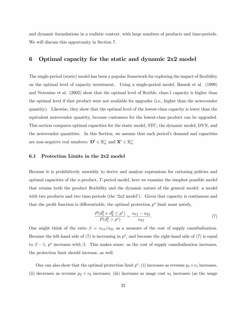
6 Optimal capacity for the static and dynamic 2x2 model

The single-period (static) model has been a popular framework for exploring the impact of flexibility

on the optimal level of capacity investment. Using a single-period model, Bassok et al. (1999)

and Netessine et al. (2002) show that the optimal level of flexible, class-1 capacity is higher than

the optimal level if that product were not available for upgrades (i.e., higher than the newsvendor

quantity). Likewise, they show that the optimal level of the lowest-class capacity is lower than the

equivalent newsvendor quantity, because customers for the lowest-class product can be upgraded.

This section compares optimal capacities for the static model, STC, the dynamic model, DYN, and

the newsvendor quantities. In this Section, we assume that each period’s demand and capacities

are non-negative real numbers: Dt ∈ R+n and Xt ∈ R+n .

6.1 Protection Limits in the 2x2 model

Because it is prohibitively unwieldy to derive and analyze expressions for rationing policies and

optimal capacities of the n-product, T -period model, here we examine the simplest possible model

that retains both the product flexibility and the dynamic nature of the general model: a model

with two products and two time-periods (the ‘2x2 model’). Given that capacity is continuous and

that the profit function is differentiable, the optimal protection p∗ limit must satisfy,

P (d21 + d22 ≤ p∗)

P (d21 > p∗)

=α11 − α21

α21. (7)

One might think of the ratio β = α11/α21 as a measure of the cost of supply cannibalization.

Because the left-hand side of (7) is increasing in p∗, and because the right-hand side of (7) is equal

to β − 1, p∗ increases with β. This makes sense: as the cost of supply cannibalization increases,

the protection limit should increase, as well.

One can also show that the optimal protection limit p∗, (i) increases as revenue p1+v1 increases,

(ii) decreases as revenue p2 + v2 increases, (iii) increases as usage cost u1 increases (as the usage

22

cost u1 rises, the firm is less willing to release expensive capacity to less-lucrative customers), and

(iv) increases as second-period demand for either product rises (according to the usual stochastic

order). See Shumsky and Zhang (2003) for details.

6.2 Optimal Capacities in the 2x2 model

One might think of the static model is a best case, for the firm is able to gather all demand

information and then allocate capacity optimally. Because in the dynamic model the firm is forced

to make allocation decisions before all customers have arrived, flexibility may not be used optimally.

Therefore, a reasonable prediction is that the solution to the dynamic model should have smaller

investments in the highest-class capacity and larger investments in the lowest-class capacity, as

compared to the static model. In general, our analysis and numerical experiments confirm this

prediction, although there can be exceptions. In fact, given certain parameters, it may be optimal

to have more class-1 capacity in the dynamic case than in the static case.

Recall that the objective function of the static model, ΠSTC(x1, x2), is defined in equation (2)

and that the dynamic model, ΠDYN(x1, x2), is defined in equation (1). Let (xSTC1 , xSTC2 ) and

(xDYN1 , xDYN2 ) be the optimal capacities for each of these models. Appendix C contains explicit

formulations for these models as well as first-order conditions for the optimal capacities. These

first-order conditions lead to the following result, and the proof of this Proposition is also included

in Appendix C.

Proposition 7 In the 2x2 case, ∂ΠDYN(x1, x2)/∂x2 ≥ ∂ΠSTC(x1, x2)/∂x2 for any capacities x1

and x2.

Proposition 7 indicates that the marginal value of an additional unit of type-2 inventory is more

valuable in the dynamic environment than in the static environment. The terms of the partial

derivative ∂ΠDYN(x∗1, x∗2)/∂x2 in Appendix C suggest why: extra type-2 capacity can be useful for

protecting against ‘supply cannibalization,’ upgrades of type-2 customers in the first period that

lead to a shortage of type-1 capacity for type-1 customers in the second period. While Proposition 7

is not sufficient to show that xDYN2 ≥ xSTC2 , we have conducted thousands of numerical experiments

23

using a wide variety of parameters and two types of distribution functions (truncated normal and

uniform), and in every case, xDYN2 ≥ xSTC2 . We describe examples of these experiments below.

There is no analogue of Proposition 7 for type-1 capacity: ∂ΠDYN/∂x1 ≶ ∂Π/∂x1. In addition,

we will see examples below in which xDYN1 ≤ xSTC1 and xDYN1 > xSTC1 .

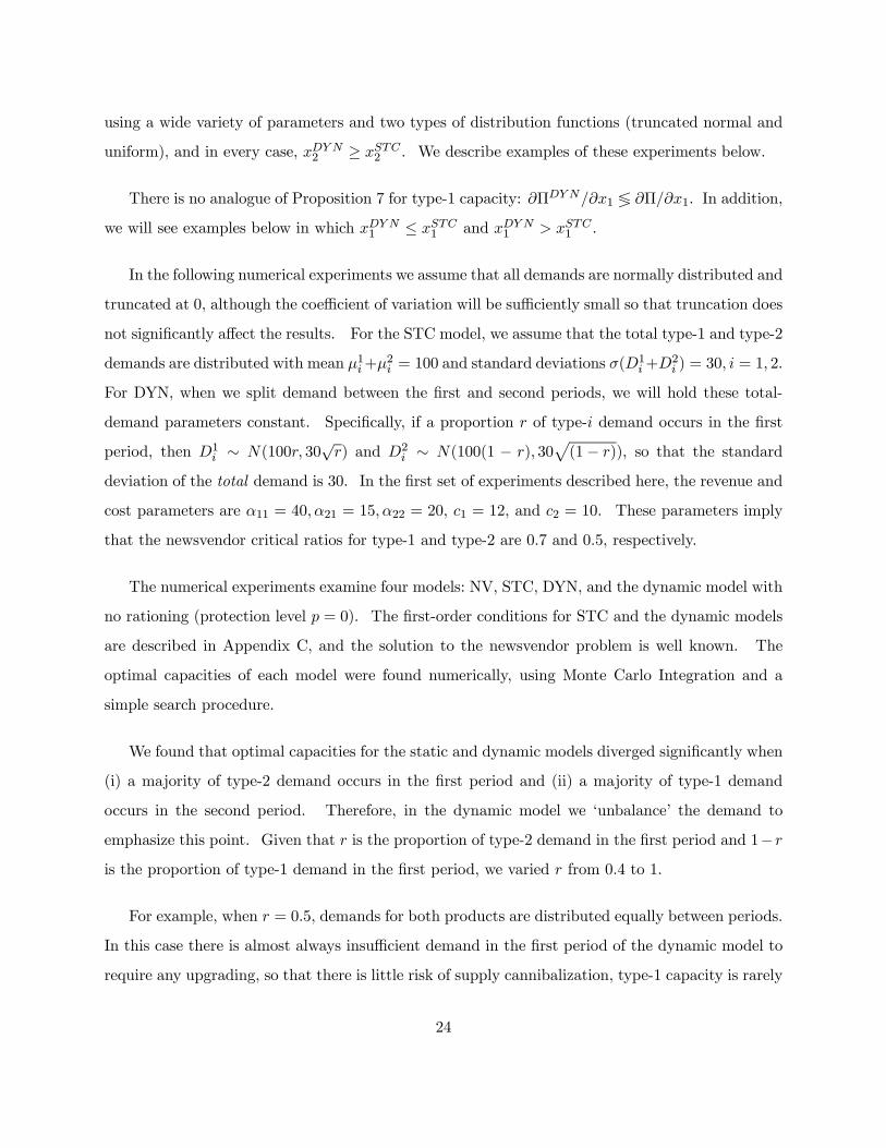
In the following numerical experiments we assume that all demands are normally distributed and

truncated at 0, although the coefficient of variation will be sufficiently small so that truncation does

not significantly affect the results. For the STC model, we assume that the total type-1 and type-2

demands are distributed with mean µ1i+µ2i = 100 and standard deviations σ(D

1i+D

2i ) = 30, i = 1, 2.

For DYN, when we split demand between the first and second periods, we will hold these total-

demand parameters constant. Specifically, if a proportion r of type-i demand occurs in the first

period, then D1i ∼ N(100r, 30√r) and D2i ∼ N(100(1 − r), 30p(1− r)), so that the standard

deviation of the total demand is 30. In the first set of experiments described here, the revenue and

cost parameters are α11 = 40,α21 = 15,α22 = 20, c1 = 12, and c2 = 10. These parameters imply

that the newsvendor critical ratios for type-1 and type-2 are 0.7 and 0.5, respectively.

The numerical experiments examine four models: NV, STC, DYN, and the dynamic model with

no rationing (protection level p = 0). The first-order conditions for STC and the dynamic models

are described in Appendix C, and the solution to the newsvendor problem is well known. The

optimal capacities of each model were found numerically, using Monte Carlo Integration and a

simple search procedure.

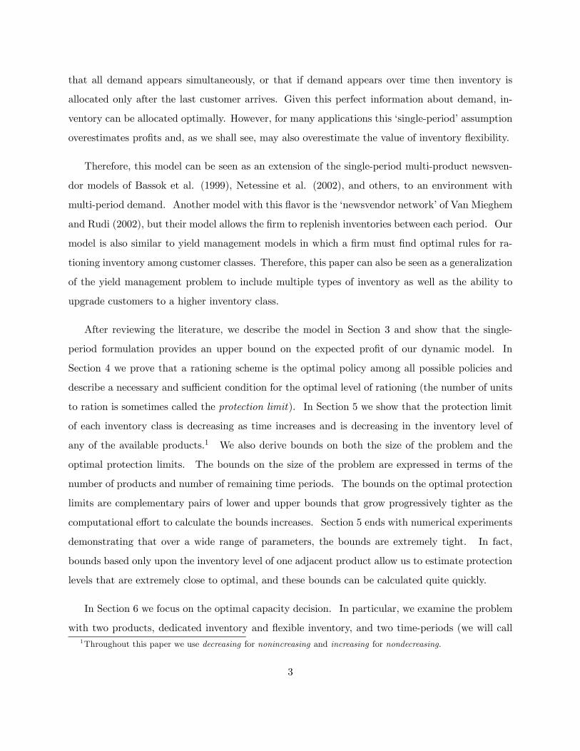
We found that optimal capacities for the static and dynamic models diverged significantly when

(i) a majority of type-2 demand occurs in the first period and (ii) a majority of type-1 demand

occurs in the second period. Therefore, in the dynamic model we ‘unbalance’ the demand to

emphasize this point. Given that r is the proportion of type-2 demand in the first period and 1−ris the proportion of type-1 demand in the first period, we varied r from 0.4 to 1.

For example, when r = 0.5, demands for both products are distributed equally between periods.

In this case there is almost always insufficient demand in the first period of the dynamic model to

require any upgrading, so that there is little risk of supply cannibalization, type-1 capacity is rarely

24

40 50 60 70 80 90 100114

116

118

120

122

124

126

128

% type-2 demand in 1st period, % type-1 demand in 2nd period

Opt

imal

type

-1 c

apac

ity

static

dynamic,optimal rationing

dynamic, no rationing

newsvendor

40 50 60 70 80 90 100114

116

118

120

122

124

126

128

% type-2 demand in 1st period, % type-1 demand in 2nd period

Opt

imal

type

-1 c

apac

ity

static

dynamic,optimal rationing

dynamic, no rationing

newsvendor

Figure 1: Optimal type-1 capacity

rationed, the particular rationing policy does not matter, and there is little difference between the

static and dynamic models. However, as r rises, the early appearance of type-2 demand and the

late appearance of type-1 demand forces the firm to either upgrade type-2 demand or ration type-1

products. The model with r = 1 is analogous to the standard yield management problem, in which

low-fare passengers arrive first, followed by high-fare passengers.

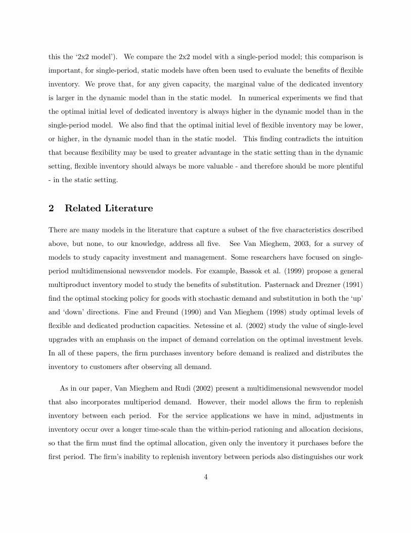
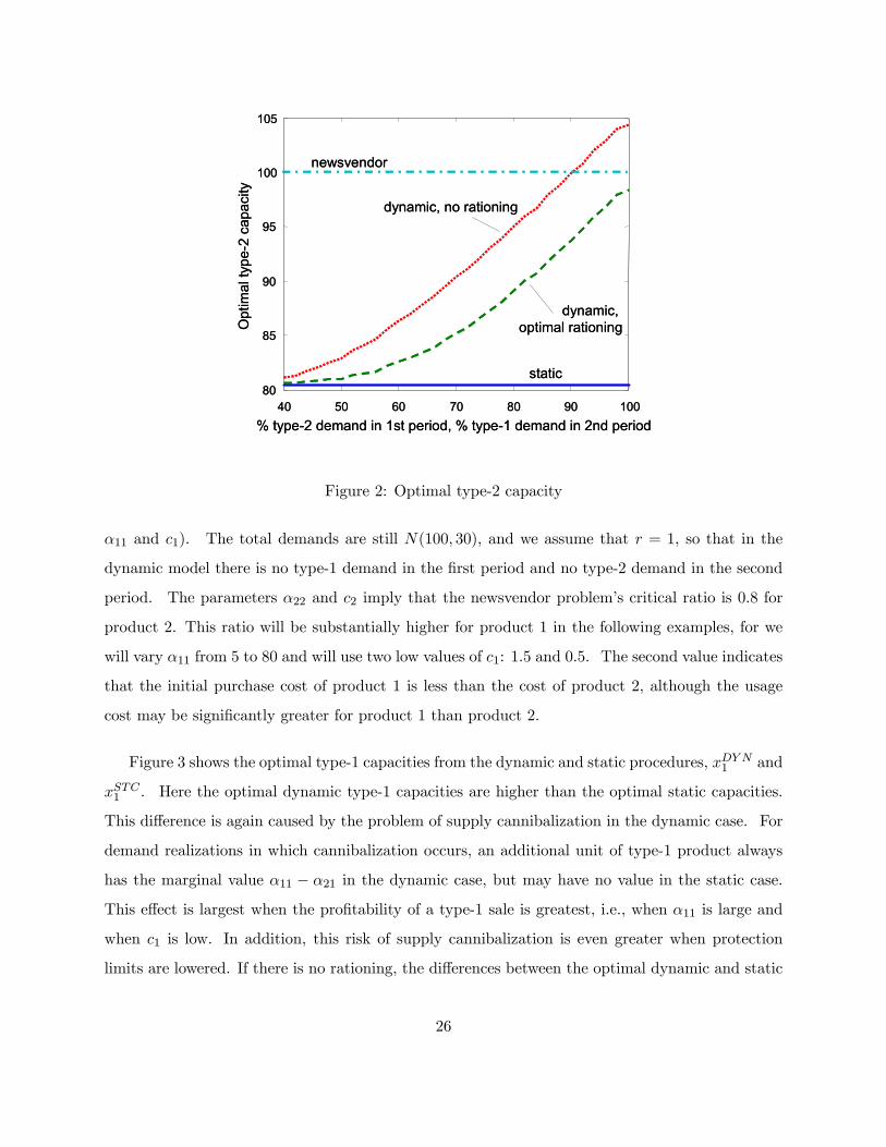
Figures 1 and 2 show the optimal type-1 and type-2 capacity values, respectively, for each model.

In Figure 1 the dynamic model’s optimal type-1 capacity, xDYN1 is consistently below the optimal

capacity from the static model, xSTC1 , although we have found that the opposite can be true (see

below). A more pronounced pattern is shown in Figure 2, where we see that the optimal type-2

capacities can be significantly higher in the dynamic model (xDYN2 ≥ xSTC2 ). The extra type-2

capacity acts as a buffer to prevent cannibalization of more lucrative type-1 capacity. This role

for type-2 capacity is particularly important when there is no rationing, thus inflating the optimal

type-2 capacity.

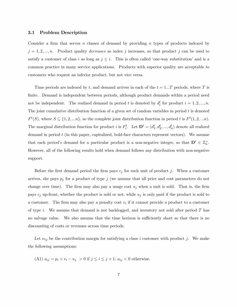
To see that it is possible to have xDYN1 > xSTC1 , consider an experiment with the following

revenue and cost parameters: α21 = 4,α22 = 5, and c2 = 1 (we will try a variety of values for both

25

40 50 60 70 80 90 10080

85

90

95

100

105

% type-2 demand in 1st period, % type-1 demand in 2nd period

Opt

imal

type

-2 c

apac

ity

static

dynamic, optimal rationing

dynamic, no rationing

newsvendor

40 50 60 70 80 90 10080

85

90

95

100

105

% type-2 demand in 1st period, % type-1 demand in 2nd period

Opt

imal

type

-2 c

apac

ity

static

dynamic, optimal rationing

dynamic, no rationing

newsvendor

Figure 2: Optimal type-2 capacity

α11 and c1). The total demands are still N(100, 30), and we assume that r = 1, so that in the

dynamic model there is no type-1 demand in the first period and no type-2 demand in the second

period. The parameters α22 and c2 imply that the newsvendor problem’s critical ratio is 0.8 for

product 2. This ratio will be substantially higher for product 1 in the following examples, for we

will vary α11 from 5 to 80 and will use two low values of c1: 1.5 and 0.5. The second value indicates

that the initial purchase cost of product 1 is less than the cost of product 2, although the usage

cost may be significantly greater for product 1 than product 2.

Figure 3 shows the optimal type-1 capacities from the dynamic and static procedures, xDYN1 and

xSTC1 . Here the optimal dynamic type-1 capacities are higher than the optimal static capacities.

This difference is again caused by the problem of supply cannibalization in the dynamic case. For

demand realizations in which cannibalization occurs, an additional unit of type-1 product always

has the marginal value α11 − α21 in the dynamic case, but may have no value in the static case.

This effect is largest when the profitability of a type-1 sale is greatest, i.e., when α11 is large and

when c1 is low. In addition, this risk of supply cannibalization is even greater when protection

limits are lowered. If there is no rationing, the differences between the optimal dynamic and static

26

2 4 6 8 10 12 14 16 18 20120

130

140

150

160

170

180

190

200

210

α11/α21

Type

-1 c

apac

itystatic

dynamic, optimal rationing

c1/c2=1.5

static

dynamic, optimal rationing

c1/c2=0.5

2 4 6 8 10 12 14 16 18 20120

130

140

150

160

170

180

190

200

210

α11/α21

Type

-1 c

apac

itystatic

dynamic, optimal rationing

c1/c2=1.5

static

dynamic, optimal rationing

c1/c2=0.5

Figure 3: Optimal type-1 capacity can be larger in the dynamic model

capacities are consistently larger than the differences seen in Figure 3.

7 Conclusions and Further Research

In this paper we formulate a flexible capacity investment and allocation problem in which demand

arrives over a sequence of discrete time intervals. Because total demand from the most lucrative

customers is uncertain when inventory allocation decisions must be made, the firm may hold back,

or ration, some products before the last time interval. We show that the optimal assignment

policy involves two steps: greedy allocation, followed by upgrading that is limited by a protection

limit. We show that the protection limits satisfy certain reasonable properties: the protection

limits decrease as inventories increase, and the protection limits decrease over time. We use these

properties to derive simple bounds on the protection limits.

Previous work on capacity investment decisions and the impact of flexibility have focused on

static models. Previous results have shown that the optimal quantity of flexible (dedicated)

capacity is higher (lower) than the optimal newsvendor quantities. We have found that for the

27

2x2 dynamic model, the optimal capacities can be pushed back toward the newsvendor quantities,

although there are cases in which the optimal level of flexible capacity can be greater in the dynamic

case than in the static case. We have also seen that the ordering of demand arrival is a significant

factor, for differences between the static and dynamic model are greatest when low-class demand

tends to arrive first and high-class demand arrives later.

Given the promising results showing that the bounds can lead to accurate approximations of

the optimal protection levels, we expect to use heuristic protection levels based on the bounds

(e.g., the average of the bounds) to examine problems with large numbers of periods and products.

Using these heuristics, we will explore the impact on total expected profit of reducing the number

of demand periods, which is roughly equivalent to gathering advance demand information. We

will also examine the consequences of using sub-optimal policies, such as a greedy policy (‘upgrade

whenever possible’) and a no-upgrade policy that separates the problem into simple newsvendor

problems. Finally, the heuristics may allow us to consider optimal capacity levels for problems

larger than the 2X2 problem of Section 6.

There are also many possible extensions to the model, such as the inclusion of backlogging

or discounting, and incorporating inter-period demand dependence that would allow the firm to

update protection levels as demand arrives. Determining the actual values of optimal booking

limits can be difficult, particularly in problems with large numbers of flexible products and time

periods, so that recursive and/or heuristic methods for finding booking limits would be useful.

Finally, in many real-world environments customer arrivals cannot be divided into time-periods,

and an important extension of the analysis would be to compare our dynamic model with a model

that features continuous arrivals (e.g., type-1 and 2 customers arrive according to a Poisson or

diffusion process). However, the multi-period model approximates a continuous models as the

number of periods increases. In addition, a model with a small number of discrete demand periods

may be reasonable approximation when different customer classes tend to arrive in different periods,

as is often the case in yield management applications.

Appendix A: Proposition 3

Proof : From Lemma 1 we know that rationing decisions within the subproblem involve only

28

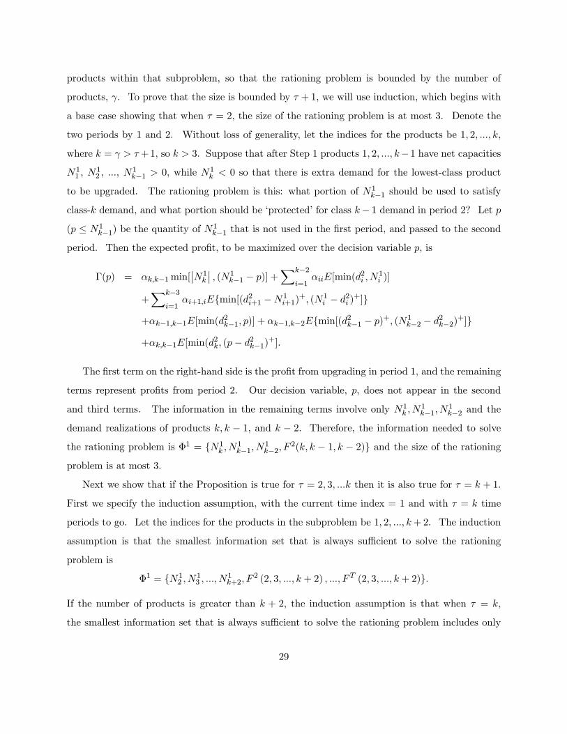
products within that subproblem, so that the rationing problem is bounded by the number of

products, γ. To prove that the size is bounded by τ + 1, we will use induction, which begins with

a base case showing that when τ = 2, the size of the rationing problem is at most 3. Denote the

two periods by 1 and 2. Without loss of generality, let the indices for the products be 1, 2, ..., k,

where k = γ > τ +1, so k > 3. Suppose that after Step 1 products 1, 2, ..., k−1 have net capacitiesN11 , N

12 , ..., N

1k−1 > 0, while N1

k < 0 so that there is extra demand for the lowest-class product

to be upgraded. The rationing problem is this: what portion of N1k−1 should be used to satisfy

class-k demand, and what portion should be ‘protected’ for class k− 1 demand in period 2? Let p

(p ≤ N1k−1) be the quantity of N

1k−1 that is not used in the first period, and passed to the second

period. Then the expected profit, to be maximized over the decision variable p, is

Γ(p) = αk,k−1min[¯̄N1k

¯̄, (N1

k−1 − p)] +Xk−2

i=1αiiE[min(d

2i , N

1i )]

+Xk−3

i=1αi+1,iE{min[(d2i+1 −N1

i+1)+, (N1

i − d2i )+]}+αk−1,k−1E[min(d2k−1, p)] + αk−1,k−2E{min[(d2k−1 − p)+, (N1

k−2 − d2k−2)+]}+αk,k−1E[min(d2k, (p− d2k−1)+].

The first term on the right-hand side is the profit from upgrading in period 1, and the remaining

terms represent profits from period 2. Our decision variable, p, does not appear in the second

and third terms. The information in the remaining terms involve only N1k , N

1k−1, N

1k−2 and the

demand realizations of products k, k − 1, and k − 2. Therefore, the information needed to solvethe rationing problem is Φ1 = {N1

k , N1k−1, N

1k−2, F

2(k, k − 1, k − 2)} and the size of the rationingproblem is at most 3.

Next we show that if the Proposition is true for τ = 2, 3, ...k then it is also true for τ = k + 1.

First we specify the induction assumption, with the current time index = 1 and with τ = k time

periods to go. Let the indices for the products in the subproblem be 1, 2, ..., k+2. The induction

assumption is that the smallest information set that is always sufficient to solve the rationing

problem is

Φ1 = {N12 , N

13 , ..., N

1k+2, F

2 (2, 3, ..., k + 2) , ..., FT (2, 3, ..., k + 2)}.

If the number of products is greater than k + 2, the induction assumption is that when τ = k,

the smallest information set that is always sufficient to solve the rationing problem includes only

29

the ‘bottom’ k + 1 products. Therefore, the size of the problem with τ = k is at most k + 1 and

product 1 is not included in the information set Φ1.

Now consider the problem with τ = k + 1 and product indices 1, 2, ..., k + 3 (again, it is easy

to extend this logic when the number of products is greater than k + 3). In the first period,

the remaining capacity after Step 1 is (N11 , N

12 , ..., N

1k+2, N

1k+3), where N

1i > 0 for 1 ≤ i ≤ k +

2 but N1k+3 < 0. We want to show that the size of this problem is k + 2. As in the base

case, the objective function for the rationing problem includes the profit in the current period,

αk+3,k+2min[¯̄N1k+3

¯̄, (N1

k+2 − p)], plus expected profits from the subproblem in future periods.

Given that there are k+ 3 products, the proof is complete if we can show that product N11 and its

future demands d21, d31, ...d

T1 will have no influence on the rationing decision in the current period.

This implies that product 1 is not included in the information set Φ1, and therefore the size of the

rationing problem is limited by the remaining k + 2 products.

After making the upgrade decision for period 1, we calculate the capacities available for period

2, observe realized demand in period 2, and perform the parallel allocation in Step 1. For this new

subproblem three scenarios are possible: (i) At least one class of product of a higher class than

k + 2 runs out in period 2: N2i < 0 for some i = 1, ..., k + 1. Then the problem splits into two

subproblems and product 1 will have no impact on the rationing made in period 1; (ii) All classes

higher than k + 2 have extra capacity (N2i > 0, i = 1, ..., k + 1), but N2

k+2 < 0. From this point

on, demand for product k + 3 cannot be filled and product k + 3 drops out of the subproblem.

Therefore, the new period-2 subproblem is identical to the subproblem in the induction assumption:

τ = k,and the subproblem includes only products 1, 2, ...k + 2. Let Φ2 be the information set for

this period-2 rationing problem. From the induction assumption, Φ2 does not include product 1,

and therefore product 1 is not included in Φ1; (iii) N2i > 0, i = 1, ..., k + 2. In this case, we still

have a rationing problem with demand from products i = 1, ..., k + 3 and supply from products

i = 1, ..., k + 2, but now with τ = k. The induction assumption states that Φ2 includes only the

‘bottom’ k+1 products, i = 3, ..., k+3. Therefore, Φ2 does not include product 1, and neither does

Φ1. ¥

Appendix B: Monotonicity resultsProposition 4 The optimal protection limit ept is decreasing in the inventory vector Xt.

30

Proof : Consider two subproblems in time period t, and without loss of generality assume that

the subproblem’s product indices are 1, ..., k+1. Before step 1, the first subproblem has inventories

Xt, where xti > 0, i = 1, ..., k, and xtk+1 = 0. The second subproblem has inventories bXt = Xt + ej

with 1 ≤ j ≤ k − 1. Let ∆tk(Xt) be the marginal value of an additional unit of product k intime-period t, given inventory Xt. To prove that the proposition is true, we proceed by backwards

induction, with two induction assumptions: (i) the optimal protection limit ept is decreasing inthe inventory vector Xt (this is the Proposition) and (ii) in the next time-period, the marginal

value of product k is decreasing in the capacity vector. That is, ∆t+1k (bXt+1) ≤ ∆t+1k (Xt+1) forbXt+1 = Xt+1 + ej , 1 ≤ j ≤ k − 1.Before showing that the induction assumptions are true for all t, we first prove that assumption

(ii) implies (i). Recall that the protection limit ept solves a concave optimization problem in one

variable, with the solution specified by condition (6). The left-hand-side of (6) is the marginal

value of an increase in the quantity of product k made available in the next period. Therefore, the

protection limit rises or falls as the marginal value of product k in the next period rises or falls.

Furthermore, if bXt = Xt+ ej for some 1 ≤ j ≤ k− 1, then bxt+1j ≥ xt+1j , because the extra capacity

of the higher-level product is either passed along or used to satisfy demand in period t. Therefore,

given induction assumption (ii), an increase in Xt may lead to a decrease in the marginal value of

product k in the next period, and ept is decreasing in Xt.Now consider the rationing problem at time T . Netessine et al. (2002) show that the profit

function of the single-period model with one-step upgrading is submodular in its capacity X. In

other words, the marginal value of a product is decreasing in the quantity of any other product.

Therefore, ∆Tk (bXT ) ≤ ∆Tk (XT ) for bXT = XT + ej , 1 ≤ j ≤ k − 1. From the discussion in the last

paragraph, this also implies that the optimal protection limit epT−1 is decreasing in the inventoryvector XT−1.

Assume that induction assumptions (i) and (ii) hold for periods t and t+1, respectively, and we

will show that (ii) is true for t and therefore (i) is true for t− 1. Given a realization of demand inperiod t, Dt, after Step 1 we are left with the net capacity vectors Nt = Xt−Dt and N̂t = bXt−Dt

(note Nt and N̂t only differ in the jth element, and by one unit). To find the marginal value of

31

an extra unit of product k, we must consider a variety of scenarios. In each of these cases, an

extra unit of product k may be used for one of three things. The unit may be used for a parallel

assignment to a customer of class k (denoted by ‘ k−→’ and ‘ bk−→’ given Nt and N̂t, respectively), it

may be used to upgrade a customer of class k + 1 (denoted ‘k + 1−−−→’ and ‘[k + 1−−−→’) and it may not beused in period t but passed along to period t+ 1 (denoted ‘t+ 1−−→’ and ‘[t+ 1−−→’). Before cataloguingan exhaustive list of scenarios, we consider the following observation:

Observation: Suppose that in period t, N tk > 0, and that the extra unit of product k is not

allocated in period t but is passed along to the next period (‘t+ 1−−→’). Then one of the following

must be true:

Case A: We have the event t+ 1−−→ because all excess type-(k + 1) demand has been upgraded

and the protection limit has not yet been reached. In this case ∆tk(Xt) ≤ αk+1,k because the

quantity of available capacity is larger than the protection limit.

Case B: We have the event t+ 1−−→ even though there is still excess type-(k + 1) demand to be

upgraded. In this case, the protection limit has been reached. Here we can also make a somewhat

surprising conclusion: there were no upgrades in period t. This can be shown by contradiction.

Suppose that there were upgrades in period t. Then there was one type-(k + 1) customer who

hit the protection limit during the period and was not upgraded. But if we add an extra unit of

type-k product, then this unit will be used to upgrade that customer, and we have k + 1−−−→, insteadof the assumed event, t+ 1−−→. Also, in this case, ∆

tk(X

t) ≥ αk+1,k because the protection limit has

been reached.

The same reasoning can be applied when we have residual capacity N̂t and event [t+ 1−−→: onlyCase A and Case B are possible.

Now we are ready to list all possible sample paths and examine, for each path, the marginal

value of an extra unit of product k given inventories Xtand bXt. We begin by looking at a relativelysimple case in which our subproblem ‘splits’ because we run out of capacity for a high-level product:

(1) N̂ ti ≤ 0 for some j ≤ i ≤ k − 1, so that the demand for some product in the chain between

j and k − 1 is greater than the corresponding capacity bXt (thus also Xt). Then, the allocation

32

problem separates in period t+ 1 and the one extra unit of product j in bXt has no impact on themarginal value of product k. Therefore, ∆tk(bXt) = ∆tk(Xt).

(2) For the remaining scenarios we assume that N̂ ti > 0 for all j ≤ i ≤ k−1. We define subcases

according to the value of N̂ tk = N

tk, the amount of product k available after Step 1. We consider

(2.1) N̂ tk ≥ 0 and (2.2) N̂ t

k < 0. Unfortunately, each of these cases will also have subcases, and

subsubcases!

(2.1) N̂ tk = N t

k ≥ 0. Here there are two subcases, N tk+1 = 0 and N t

k+1 < 0 (we cannot have

N tk+1 > 0, according to the definition of the subproblem).

(2.1.1) If N̂ tk+1 = N t

k+1 = 0 then there will be no upgrading and N̂ tk = N t

k will be passed to

period t+ 1. Therefore, by the induction assumption, we know ∆tk(bXt) ≤ ∆tk(Xt).(2.1.2) If N̂ t

k+1 = Ntk+1 < 0, then the extra unit of product k may be used to upgrade demand

for product k + 1. This is the most complex case because the extra unit may be used differently,

given Xt and bXt (recall that the protection limit may be lower under bXt). Because N̂ tk = N

tk ≥ 0

there is no type-k demand remaining, so we cannot have k−→ or bk−→. Therefore, we have four cases:(k + 1−−−→,

[k + 1−−−→), (t+ 1−−→,[t+ 1−−→), (k + 1−−−→,[t+ 1−−→), and (t+ 1−−→,[k + 1−−−→).(2.1.2.1) (k + 1−−−→,

[k + 1−−−→): In this case, ∆tk(bXt) = ∆tk(Xt) = αk+1,k.

(2.1.2.2) (t+ 1−−→,[t+ 1−−→): From the Observation above, the same amount of product k is passed

to period t + 1 under Xt and bXt. For Case A, all demand for product k + 1 is upgraded, andthe same quantity N t

k − dtk+1 is passed to period t+ 1 under both Xt and bXt. For Case B, thereis no upgrading, so N t

k is passed to period t + 1 under both Xt and bXt. Then by the induction

assumption, we know ∆tk(bXt) ≤ ∆tk(Xt).(2.1.2.3) (k + 1−−−→,[t+ 1−−→): Here the additional unit in X

t is used for upgrading, for a marginal

value of αk+1,k. Under bXt, we are passing along the extra unit, and for Case A we know that

∆tk(bXt) ≤ αk+1,k = ∆

tk(X

t). Case B implies an upgrade occurred under Xt while the same unit of

capacity was protected under bXt, implying a larger protection limit under bXt. But the inductionassumption indicates that protection limits are decreasing undercXt. Therefore, Case B cannot

occur.

(2.1.2.4) (t+ 1−−→,[k + 1−−−→): Under Xt we again consider Case A and Case B. For Case A,

we observed that all demand must have been upgraded and that there is more inventory than the

33

protection limit. However, we also know that under bXt the protection limit is the same, or smaller,than under Xt so both t+ 1−−→ and [k + 1−−−→ cannot occur simultaneously, and Case A is impossible.

Given Case B, under bXt the extra unit of product k is used for upgrading, with marginal valueαk+1,k. Under Xt we know the marginal value of the additional unit is at least as high as αk+1,k

because the unit is passed to the next period even though there is an upgrading opportunity. Again,

we have ∆tk(bXt) ≤ ∆tk(Xt).(2.2) N̂ t

k = Ntk < 0. Because it is always optimal to complete parallel allocations (Step 1), this

case implies events k−→ and bk−→: we always assign an extra unit of product k to unmet k demand.However, to calculate the marginal value of this assignment, we have to consider whether this

‘marginal’ customer had already been satisfied by an upgrade to capacity k − 1. Therefore, weconsider four cases:

(2.2.1) For both Xt and bXt, the additional unit of product k satisfies a type-k customer whootherwise would have been turned away. In this case, ∆tk(bXt) = ∆tk(Xt).

(2.2.2) For both Xt and bXt, the additional unit of product k satisfies a type-k customer whootherwise would have been upgraded to product k − 1. In this case, ∆tk(bXt) = ∆tk(Xt).

(2.2.3) Under Xt the customer would not have been upgraded (would have been turned away),

but under bXt the additional unit of product k satisfies a type-k customer who otherwise wouldhave been upgraded to product k − 1. In this case, ∆tk(bXt) = αkk − αk,k−1 +∆t+1k−1(bXt). Becausethe last unit of product k− 1 had been used for upgrading, we know ∆t+1k−1(bXt)≤αk,k−1. Therefore,∆tk(

bXt) ≤ ∆tk(Xt) = αkk.

(2.2.4) Under the last scenario, the marginal customer would have been upgraded under Xt but

not upgraded under bXt. However, our induction assumption states that under bXt the protectionlimit is the same, or smaller, than under Xt. Therefore, this scenario cannot occur.

We have shown that for all possible scenarios ∆tk(bXt) ≤ ∆tk(Xt) and, therefore, the protectionlimit is decreasing in the state vector. ¥

Proposition 5 The optimal protection limit ept is decreasing over time.Proof : Consider two rationing problems with the same state vector N = (N1, N2, ..., Nk+1).

Let problem 1 be in period t1, while problem 2 is in period t2, and t1 < t2. Let ep1 and ep2 be theoptimal protection limits for product k in the two problems, respectively. To prove ep1 ≥ ep2 we

34

first show that the marginal value of product k, passed to the next period, is higher in problem 1

than that in problem 2. In particular, we show that this is true for any sample path between t1

and t2.

Suppose that an extra unit of product k is passed to t1+1 in problem 1 and to t2+1 in problem

2, and consider the demand arriving in problem 1 during periods t1+1 to t2. There are two possible

cases. First, if no demand for any product is satisfied during those periods. In this case, problem

1 is equivalent to problem 2 at period t2 + 1. Second, if a positive amount of demand is satisfied

during those periods. Then at period t2 + 1, the capacity vector of problem 1 is strictly smaller

than that of problem 2. By the reasoning in the proof of Proposition 4, the marginal value of a

unit of product k passed to the next period is higher for problem 1 than for problem 2. From the

rationing optimality condition (6), ep1 ≥ ep2. ¥

Appendix C: 2x2 capacity optimization and Proposition 7

Given an arbitrary protection limit p, the objective function of the dynamic 2x2 model is

ΠDYN (x1, x2)

= ED1,D2

α11min(d11, x1) + α22min(d

12, x2) + α21min

£(d12 − x2)+, (x1 − p− d11)+

¤+α11min

£d21, (x1 − d11)+ −min

£(d12 − x2)+, (x1 − p− d11)+

¤¤+α22min

£d22, (x2 − d12)+

¤+α21min

©d22 − (x2 − d12)+

ª+, (x1 − d11)+−

min£(d12 − x2)+, (x1 − p− d11)+

¤− d21+

−c1x1 − c2x2

.

The objective function of STC is

ΠSTC(x1, x2) = ED1,D2

α11min(d11 + d

21, x1) + α22min(d

12 + d

22, x2)

+α21min£(d12 + d

22 − x2)+, (x1 − d11 − d21)+

¤− c1x1 − c2x2 .

For convenience let xT = x1+x2, xT−p = x1−p+x2,and dT = d11+d12+d21+d22. Using techniquessimilar to those described by Netessine and Rudi (2002), we find the following partial derivative:

35

∂ΠDYN

∂x2=α22P (d

12 > x2)− α21P (d

12 > x2, d

11 + d

12 ≤ xT−p)

+ α11P (d12 > x2, d

11 + d

12 ≤ xT−p, d11 + d12 + d21 > xT )

+ α22P (d12 ≤ x2, d12 + d22 > x2)

+ α21P (d12 > x2, d

11 + d

12 ≤ xT−p, d11 + d12 + d21 ≤ xT , dT > xT )

− α21P (d12 ≤ x2, d12 + d22 > x2, dT ≤ xT )− c2

The third probability term with coefficient α11 merits special attention. This is the incremental

profit when an additional unit of type-2 capacity leads to fewer upgrades in the first period, and

thus more type-1 sales in the second period. This is the marginal benefit due to a reduction in the

cannibalization of capacity.

The partial derivative for the single-period problem is

∂ΠSTC

∂x2= α22P (d

12 + d

22 > x2)− α21P (d

12 + d

22 > x2, dT ≤ xT )− c2.

Proposition 7 In the 2x2 case, ∂ΠDYN(x1, x2)/∂x2 ≥ ∂ΠSTC(x1, x2)/∂x2 for any capacities

x1 and x2.

Proof : In the expression for ∂ΠDYN/∂x2 there are two probability terms multiplied by the

constant α22:

α22©P (d12 > x2) + P (d

12 ≤ x2, d12 + d22 > x2)

ª= α22P (d

12 + d

22 > x2).

Therefore, the terms with the coefficient α22 are equal in ∂ΠDYN/∂x2 and ∂ΠSTC/∂x2. In ad-

dition, both expressions include the term ‘−c2’. Let Ψ denote the remaining terms in ∂ΠDYN/∂x2(the second, third, fifth and sixth terms). We now show that Ψ is greater than or equal to the

remaining term in ∂ΠSTC/∂x2:

Ψ ≥ α21

−P (d12 + d22 > x2, dT ≤ xT )+P (d12 > x2, dT ≤ xT )−P (d12 > x2, d11 + d12 ≤ xT−p, d11 + d12 + d21 ≤ xT , dT ≤ xT )

≥ −α21P (d12 + d22 > x2, dT ≤ xT ).

36

where the first inequality follows by replacing α11 with α21 and rearranging the probability terms.

This result applies for any protection level p, including the optimal protection level p∗. Therefore,

∂ΠDYN(x1, x2)/∂x2 ≥ ∂ΠSTC(x1, x2)/∂x2. ¥

AcknowledgementsWe are grateful to William Cooper, Marshall Freimer, Serguei Netessine, Dan Zhang, two anony-

mous referees, and an associate editor for their helpful suggestions. We also thank participants at

graduate seminars at the University of Minnesota, the University of Toronto, and the University of

California, Irvine, for their comments.

References

Alstrup, J, S. Boas, O.B.G. Madsen, R.V.V. Vidal. 1986. “Booking policy for flights with two

types of passengers”, European Journal of Operational Research, 27: 274-288.

Archibald, T.W., S.A.E. Sassen, L.C. Thomas. 1997. “An optimal policy for a two depot inventory

problem with stock transfer”, Management Science, 43(2): 173-183.

Bassok, Y., R. Anupindi, R. Akella. 1999. “Single-period multiproduct inventory models with

substitution”, Operations Research, 47(4): 632-642.

Bitran, G.R. and S.M. Gilbert. 1996. “Managing hotel reservations with uncertain arrivals”,

Operations Research, 44(1): 35-49.

Brumelle, S.L. and J.I. McGill. 1993. “Airline seat allocation with multiple nested fare classes”,

Operations Research, 41(1): 127-137.

de Véricourt F., F. Karaesmen and Y. Dallery. 2001.“Assessing the Benefits of Rationing and

Scheduling Policies for a Make-to-Stock Production System”, Manufacturing and Service

Operation Management, 2 (3): 105-121.

de Véricourt F., F. Karaesmen and Y. Dallery. 2002. “Optimal Stock Allocation for a Capacitated

Supply System”, Management Science 48 (11): 1486-1501.

Eynan, Amit. 1999. “The multi-location inventory centralization problem with first-come, first-

served allocation”, European Journal of Operational Research, 114: 38-49.

37

Fine, C.H. and R.M. Freund. 1990. “Optimal investment in product-flexible manufacturing

capacity”, Management Science, 36(4): 449-466.

Frank, K.C., R. Zhang and I. Duenyas.

Ha, A.Y. 1997a. “Inventory rationing in a make-to-stock production system with several demand

classes and lost sales”. Management Science, 43: 1093-1103.

Ha, A.Y. 1997b. “Stock rationing policy for a make-to-stock production system with two priority

classes and backordering”. Naval Res. Logist. 44: 457-472.

Ha, A.Y. 2000. “Stock rationing in an M/Ek/1 make-to-stock queue”,Management Science, 46(1):

77-87.

Hoffman, A.J. 1963. “On simple linear programming problems”, V. Klee, ed., Convexity: Pro-

ceedings of Symposia in Pure Math, Vol. 7.

Jordan, W.C. and S.C. Graves. 1995. “Principles on the benefit of manufacturing process flexi-

bility”, Management Science, 41(4): 577-594.

Kapuscinski, R. and S. Tayur. 2000. “Dynamic capacity researvation in a make-to-stock environ-

ment”, Working Paper, Carnegie Mellon University.

Karaesmen and van Ryzin. 2000. “Overbooking with substitutable inventory classes”, Working

Paper, Columbia University.

Karmarkar, U.S. 1981. “The multiperiod multilocation inventory problem”, Operations Research,

29: 215-228.

McGill, J. and van Ryzin. 1999. “Revenue management: research overview and prospects”,

Transportation Science, Vol. 33, No. 2, pgs. 233-256.

Netessine, S., G. Dobson, R.A. Shumsky. 2002. “Flexible service capacity: optimal investment

and the impact of demand correlation”, Operations Research, Vol. 50, No. 2, pgs. 375-388.

Netessine, S., and N. Rudi. 2002. “Centralized and competitive inventory models with substi-

tution”, forthcoming in Operations Research, available at

38

http://omg.ssb.rochester.edu/omgHome/Rudi/page/.

Pasternack, B.A. and Z. Drezner. 1991. “Optimal inventory policies for substitutable commodities

with stochastic demand”, Naval Research Logistics, 38: 221-240.

Porteus, E. L. 1975. “On the optimality of structured policies in countable stage decision

processes”, Management Science, 22(2), pgs. 148-157.

Robinson, L.W. 1990. “Optimal and approximate policies in multiperiod, multiproduct inventory

models with transshipment”, Operations Research, 38(2): 278-295.

Robinson, L.W. 1995. “Optimal and approximate control policies for airline booking with sequen-

tial nonmonotonic fare classes”, Operations Research, 43(2): 252-263.

Rockafellar, R. T. 1970. Convex Analysis. Princeton University Press, Princeton, New Jersey.

Savin, S.V., M.A. Cohen, N. Gans, and Z. Katalan. 2004. “Capacity management in rental

businesses with heterogeneous customer bases”, forthcoming in Operations Research.

Shumsky, R.A., and F. Zhang. 2003. “Dynamic capacity management with substitution: working

paper”, Simon School, University of Rochester.

Subramanian, J., S. Stidham, and C.J. Lautenbacher. 1999. “Airline yield management with

overbooking, cancellations, and no-shows”. Transportation Science, 33(2): 147-167.

Topkis, D.M. 1968. “Optimal ordering and rationing policies in a nonstationary dynamic inven-

tory model with n demand classes”. Management Science, 15(3): 160-176.

Van Mieghem, J.A. 1998. “Investment strategies for flexible resources”, Management Science,

44(8): 1071-1078.

Van Mieghem, J.A. and N. Rudi. 2002. “Newsvendor networks: dynamic inventories and capaci-

ties management with discretionary pooling”, Manufacturing & Service Operations Manage-

ment, 4(4): 313-335.

Van Mieghem, J. A. 2003. “Capacity Management, Investment, and Hedging: Review and Recent

Developments”, Manufacturing & Service Operations. Vol. 4, No. 4.

39

Van Slyke R. and R. Wets. 1966. “Programming under uncertainty and stochastic optimal

control”, SIAM Journal on Control, 4(1): 179-193.

Zhao, W. and Y.S. Zheng. 2001. “A dynamic model for airline seat allocation with passenger

diversion and no-shows”. Transportation Science, 35(1): 80-98.

40