efficient factor garch models and factor-dcc...
TRANSCRIPT

Quantitative Finance To apear
Efficient Factor GARCH Models and Factor-DCC Models
Kun Zhang [email protected]
Laiwan Chan [email protected]
Department of Computer Science and Engineering
The Chinese University of Hong Kong
Hong Kong
Abstract
We reveal that in the estimation of univariate GARCH or multivariate generalized or-
thogonal GARCH (GO-GARCH) models, maximizing the likelihood is equivalent to
making the standardized residuals as independent as possible. Based on that, we pro-
pose three factor GARCH models in the framework of GO-GARCH: independent-factor
GARCH exploits factors that are statistically as independent as possible; factors in
best-factor GARCH have the largest autocorrelation in their squared values such that
their volatilities could be forecasted well by univariate GARCH; factors in conditional-
decorrelation GARCH are conditionally as uncorrelated as possible. A two-step method
for estimating these models is introduced, and it gives easy and reliable estimation.
Since the extracted factors may still have weak conditional correlations, we further pro-
pose factor-DCC models, as an extension to the above factor GARCH models with
dynamic conditional correlation (DCC) modelling the remaining conditional correla-
tions between factors. Experimental results on the Hong Kong stock market shows that
conditional-decorrelation GARCH and independent-factor GARCH have better gener-
alization performance than the original GO-GARCH, and that conditional-decorrelation
GARCH (among factor GARCH models) and its extension with DCC embedded (among
factor-DCC models) behave best.
Keywords: Factor GARCH model, Mutual information, Mutual independence, Condi-
tional uncorrelatedness, Autocorrelation, Dynamic conditional correlation
1
1. Introduction
It has been over 20 years since the autoregressive conditional heteroscedasticity (ARCH) model
was proposed (Engle, 1982). A natural and powerful extension of the ARCH model is the gen-
eralized ARCH (GARCH) model (Bollerslev, 1986). These models have been shown to be very
useful in modelling and forecasting the volatility of financial return series. Furthermore, financial
assets may be inter-correlated, and their correlations play an important role in financial manage-
ment, such as portfolio construction. It was then natural to generalize the GARCH models from
modelling the conditional variance of a univariate series to modelling the conditional covariance
matrix of multivariate series (Bollerslev et al., 1988); for a recent survey on multivariate GARCH
model, see Bauwens et al. (2006).
Conventionally univariate and multivariate GARCH models are estimated by maximum like-
lihood (ML) estimation, or quasi maximum likelihood (QML) estimation, which simply assumes
that the returns are conditionally normally distributed. The maximum likelihood of GARCH mod-
els is actually closely related to statistical dependence in standardized residuals.i In the literature,
after estimating univariate GARCH models, some statistical tests, such as the BDS test (Brock
et al., 1996), can be used to test the independence of standardized residuals, so that we can com-
pare the behavior of different formulations for the GARCH model. In this work, we reveal the
relationship between the mutual information of standardized residuals and the likelihood value
attained by GARCH models. We show that in the estimation of GARCH models, maximizing the
likelihood is equivalent to minimizing the mutual information of standardized residuals. Actually,
when we use different GARCH models to fit the given data, the likelihood is a direct indicator of
how independent the standardized residuals are.
Usually multivariate GARCH models involve quite a lot of parameters, and they are difficult
to estimate for high-dimensional data (Bauwens et al., 2006). Factor GARCH models (e.g., Engle
et al., 1990; Alexander, 2000; van der Weide, 2002) provide one way to efficiently parameterize
the GARCH model. In this paper, by considering the generalized orthogonal GARCH (GO-
GARCH) model (van der Weide, 2002) from an information-theoretic point of view, we propose
to use independent component analysis (ICA) and two other statistical methods to construct fac-
tor GARCH models in the framework of GO-GARCH. The proposed models can all be estimated
easily in two separate steps. In the first step the factors are estimated according to some statis-
tical criteria. In the second step we estimate the univariate GARCH model for each factor and
i. In the GARCH literature, the innovation normalized by its time-varying standard deviation is
defined as the standardized residual.
2

construct the conditional covariance matrix of return series. Due to the simplicity and efficiency
of parameter estimation, these models are suitable for high-dimensional data. Since the extracted
factors may still have weak conditional correlations, we show that the estimate of conditional
correlations between returns can be further improved by modelling the remaining time-varying
conditional correlations between factors with the dynamic conditional correlation (DCC) model.
This leads to factor-DCC models.
This paper is organized as follows. In Section 2 we show the relationship between statistical
dependence in standardized residuals and the data likelihood of the univariate GARCH models.
Section 3 reviews multivariate GARCH models and discusses the estimation the GO-GARCH
model by the minimization of mutual information. Three forms of factor GARCH models, which
exploit ICA and other techniques for factor extraction, are proposed and discussed in Section 4.
In Section 5 we further embed the DCC model into the factor models to improve the forecasting
performance. 10 stocks selected from Hong Kong stock market are used to compare the perfor-
mance of our proposed factor GARCH models, the orthogonal GARCH , GO-GARCH, the DCC
model, and the factor-DCC models in Section 6. Section 7 concludes this paper.
2. Estimation of Univariate GARCH Model Based on Mutual Information
2.1 Univariate GARCH Models
It is well known that financial return series are almost serially uncorrelated, but the squares of
the returns are often strongly correlated, as indicated by the phenomenon of volatility clustering.
Based on these facts, one can see that the return series are not serially independent, and that
the dependency in the return series is demonstrated by the autocorrelation of the squared values.
Consequently, the return magnitude is predictable to some extent.
Inspired by volatility clustering, the ARCH-type models (Engle, 1982; Bollerslev et al., 1992;
Bera & Higgins, 1993; Poon & Granger, 2003) were proposed to model the volatility of the return
series. A popular one is the GARCH(p,q) model (Bollerslev, 1986), which is described by the
following system,
rt = ut + εt, (1)
εt =√
htzt, (2)
ht = w +q∑
i=1
αiε2t−i +
p∑
i=1
βiht−i, (3)
where rt denotes the return at time t, ut denotes the conditional mean of rt conditional on infor-
mation at time t−1 and can be described by any type of regression models, εt is the innovation, ht
3

is the conditional variance of rt based on information up through time t−1, zt is i.i.d. with mean
zero and variance one, and restrictions w > 0, αi ≥ 0, and βi ≥ 0 are imposed to ensure that
ht is positive (actually the restrictions on parameters may be weaker, see Nelson & Cao, 1992).
In Engle’s original ARCH model (Engle, 1982), zt is assumed to be Gaussian distributed. The
main approach to parameter estimation in GARCH models is based on ML estimation. Although
there is a lot of empirical evidence that the standardized residual zt does not follow the Gaussian
distribution, the normality of zt is often assumed and produces the QML estimates (Bollerslev &
Wooldridge, 1992).
2.2 Estimation of Univariate GARCH Model by Mutual Information Minimization
Parameters in the GARCH models are adjusted to capture the autocorrelation in squared returns,
which reflects the dependency in the return series. Consequently, after eliminating the effect the
time-varying volatility modeled by GARCH models, the standardized residuals, zt, should be
much more serially independent. Therefore, we can estimate the parameters in GARCH models
by making zt serially as independent as possible. The statistical dependence can be measured by
mutual information.
Mutual information is a natural and canonical measure of statistical dependence. In informa-
tion theory, the mutual information between n random variables y1, ..., yn is defined as
I(Y1, ..., Yn) =n∑
i=1
H(Yi)−H(Y), (4)
where Y = (Y1, ..., Yn)T , and H(·) denotes the (differential) entropy, defined as H(X) =
− ∫p(x) log p(x)dx (Cover & Thomas, 1991). I(Y1, ..., Yn) is always non-negative, and is zero
if and only if yi are mutually independent. Different from the coefficient of linear correlation,
which measures the linear dependency between two variables, mutual information can capture
both linear and nonlinear dependence, with no need to specify any form of dependency. Mu-
tual information has been applied to detect the dependency or to examine the predictability of
financial time series (Dionısio et al., 2003; Darbellay & Wuertz, 2000; Maasoumi & Racine,
2002).
In the GARCH(p,q) model (Eq. 1–3), we can see that the standardized residual zt is a function
of εt, εt−1, · · · , denoted by
zt = f(εt, εt−1, ...; θ), (5)
where θ is the parameter set containing the parameters in the GARCH formulation. In particular,
for the GARCH(p,q) model (Eq. 3), θ = {w, α1, ..., αq, β1, .., βp}. Bollerslev (1986) showed that
4

the necessary and sufficient condition for zt to be covariance stationary is∑q
i=1 αi +∑p
i=1 βi <
1. Under this condition, the effect of εt−k on ht (and zt) diminishes as k increases.
Denote by z∗ the vector consisting of zt at different time indices, i.e. z∗ = (zt, zt−1, ..., zt−N )T ,
and similarly for r∗ and ε∗. The dependence in the process Z , {zt} can be measured by the
mutual information rate (Taleb et al., 2001), which is defined as
I(Z) = H(zt)−H(Z), (6)
whereH(Z) = limN→∞H(z∗)N+1 is the entropy rate of the processZ (Cover & Thomas, 1991). The
mutual information rate of the process Z can also be written as I(Z) = limN→∞ 1N+1 · I(z∗).
When N is sufficiently large, we can neglect the effect of εt−N−1, εt−N−2, · · · , as they are very
early, and write Eq. 5 in matrix form:
z∗ = F(ε∗;θ), (7)
where F denotes the mapping from ε∗ to z∗. Similarly, we denote the mapping from r∗ to ε∗ by
G, i.e.
ε∗ = G(r∗; ψ), (8)
where ψ contains the parameters in the regression model for ut. The overall mapping from r∗ to
z∗ is then F ◦ G. We can estimate the parameters in the GARCH models by minimizing I(z∗),
the mutual information between components of z∗.
The Jacobian matrix of the mapping F is
JF =
∂zt∂rt
∂zt∂rt−1
· · · ∂zt∂rt−N
∂zt−1
∂rt
∂zt−1
∂rt−1· · · ∂zt−1
∂rt−N
......
. . ....
∂zt−N
∂rt
∂zt−N
∂rt−1· · · ∂zt−N
∂rt−N
=
h−1/2t
∂zt∂rt−1
· · · ∂zt∂rt−N
0 h−1/2t−1 · · · ∂zt−1
∂rt−N
......
. . ....
0 0 · · · h−1/2t−N
. (9)
Denote the determinant of JF by |JF |. Obviously |JF | =∏N
i=0 h−1/2t−i . No matter ut = 0 or is
described by a regression model, the Jacobian matrix JG is always a upper triangular matrix with
the entries on its diagonal being 1, so |JG | = 1. The determinant of the Jacobian matrix associated
with the overall transformation F ◦ G is |J| = |JF◦G | = |JF | · |JG | = |JF | =∏N
i=0 h−1/2t−i . We
then have the following relationship between the joint density pz∗(z∗) and pr∗(r∗):
pz∗(z∗) =pr∗(r∗)|J| =
pr∗(r∗)∏Ni=0 h
−1/2t−i
. (10)
As H(z∗) = −E{log pz∗(z∗)}, we further have
H(z∗) = H(r∗) + E{
logN∏
i=0
h−1/2t−i
}= H(r∗)− 1
2
N∑
i=0
E log ht−i.
5

Consequently, the mutual information rate of the process {zt} is
I(Z) = H(zt)−H(Z) = H(zt)− limN→∞
H(z∗)N + 1
= H(zt) + limN→∞
· 1N + 1
· 12
N∑
i=0
E log ht−i − limN→∞
H(r∗)N + 1
= H(zt) +12E log ht −H(R), (11)
where R denotes the process {rt}. As H(R) does not depend on the parameters θ, minimizing
I(Z) is equivalent to maximizing the following function (T denotes the number of observations)
lT (θ) = −T ·[H(zt) +
12E log ht
](12)
=T∑
t=1
log[pz(zt)]− 12
T∑
t=1
log ht, (13)
which is exactly the log-likelihood function for the observations r1, ..., rT . Note that z in Eq. 13
denotes the variable associated with zt.ii
This reveals the fact that in the estimation of univariate GARCH models, maximizing the
data likelihood is equivalent to minimizing the statistical dependence in standardized residuals.
Although these two approaches have the same objective function, we should address their distinc-
tion. In ML estimation, the density of the standardized residuals, pz , must be correctly specified
in advance. However, in practice we do not have such information exactly. QML estimation sim-
ply assumes pz to be Gaussian. In the approach based on the minimization of mutual information,
pz is not necessarily known as prior information, and it may be adaptively estimated from data
in the maximization of Eq. 13, as the so-called “semiparametric ARCH models” does in Engle
and Gonzalez-rivera (1991). Consequently this method may produce a larger likelihood value (or
more independent standardized residuals).
3. Estimation of GO-GARCH by Mutual Information Minimization
3.1 Multivariate GARCH Models
Since the financial return series may be correlated, in addition to the time-varying volatility of
each series, the time-varying correlations among them are also very useful and need to be modeled
and forecasted. For example, the time-varying correlations can help us to construct a short-term
ii. In the following we drop the time index t in the subscript to denote the variable associated
with a time series.
6
portfolio. Hence there is a need to extend the univariate GARCH models to the multivariate case.
For a survey on multivariate GARCH models, see Bauwens et al. (2006); Long (2005).
Suppose we have n return series rit, i = 1, ..., n, which form a vector rt = (r1t, ..., rnt)T .
Let εt = (ε1t, ..., εnt)T be the zero-mean version of rt, obtained by subtracting the mean from rt.
Denote the conditional covariance matrix of rt by Ht. The basic and general form for modelling
the multivariate conditional covariance matrix is the vech model (Bollerslev et al., 1988). Using
the vech operator to stack the lower triangular portion of a symmetric matrix into a column vector,
it models each element of Ht as a linear combination of the lagged squared errors, cross-products
of errors, and the lagged elements of Ht. As a special case of the vech model, the BEKK model
was proposed in Baba et al. (1991) and Engle and Kroner (1995). However, the number of
parameters in these models grows very rapidly as the data dimension increases. This causes
problems in parameter estimation when the data dimension is high.
In order to efficiently parameterize multivariate GARCH, some methods have been developed
based on univariate GARCH models, in two directions. The first is to construct the conditional co-
variance matrix by explicitly modelling both the volatility of each return series and the conditional
correlation matrix. For example, the constant conditional correlation (CCC) model of Bollerslev
(1990) assumes the conditional correlation to be constant and the time-varying behavior of con-
ditional covariances is due to the time-varying conditional variances. To relax the constant con-
ditional correlation assumption, Engle (2002), Christodoulakis and Satchell (2002), and Tse and
Tsui (2002) proposed the dynamic conditional correlation (DCC) model, the Correlated ARCH
(CorrARCH) model, and the variable conditional correlation (VCC) model, respectively. They
generalize the CCC model to allow the conditional correlation to be time dependent.
The second direction is to exploit the idea of factor models to construct multivariate GARCH
models. It is believed that there exist some common factors, which may be determined em-
pirically or constructed by some statistical methods, driving the evolution of the return series.
The idea of the multivariate factor GARCH model dates to Engle et al. (1990), in which only
a small number of common factors are empirically determined and believed to underly the ob-
served return series. In this model, the factors are not necessarily uncorrelated, and it is difficult
to determine what the factors are.
3.2 Orthogonal GARCH Models
Recently the orthogonal GARCH (O-GARCH) model was proposed by exploiting the principal
component analysis (PCA) technique to determine the factors (Ding, 1994; Alexander, 2000;
Alexander, 2001). The O-GARCH model allows n×n covariance matrices to be generated from
7

m (normally m < n) univariate GARCH processes, each of which models a principal component
of the data εt. In order to do that, we first use PCA to extract m principal components, i.e.
yt = PTmεt, where yt = (y1t, ..., ymt)T consists of the m principal components, and Pm is
a n × m matrix consisting of the eigenvectors associated with the m largest eigenvalues of the
covariance matrix of εt. Next, we use a univariate GARCH model to estimate hyit , the conditional
variance of each principal component, and construct the m × m time-varying diagonal matrix
Σt = diag{hy1t , ..., hymt}. Finally we can obtain the conditional covariance matrix of εt as
Ht = PmΣtPTm. (14)
In determining the factors in the O-GARCH model, we just use the unconditional covariance
matrix of the return series, and the conditional information is not considered. A requirement for
the validity of O-GARCH is that principal components are also conditionally uncorrelated. How-
ever, as the conditional covariance matrix of the financial return series is time-varying, the un-
conditional uncorrelatedness between principal components does not guarantee their conditional
uncorrelatedness. Recently, GO-GARCH was proposed as a generalization of O-GARCH (van
der Weide, 2002; Lanne & Saikkonen, 2005). In GO-GARCH, the orthogonality constraint of the
factor loading matrix is relaxed.
3.3 Estimation of GO-GARCH Models by Mutual Information Minimization
In GO-GARCH, the error series εt (which are the zero-mean version of the return series rt) are
assumed to be generated from some latent uncorrelated factors yt = (y1t, ..., ymt)T by linear
transformation (van der Weide, 2002):
εt = Ayt, (15)
where m ≤ n,iii yit have unit variance, and the conditional covariance matrix of yt is assumed to
be diagonal:
Σt = diag{hy1t , ..., hymt}. (16)
Each factor is described as a GARCH(1,1) process:iv
hyit = (1− αi − βi) + αiy2i,t−1 + βihyi,t−1 . (17)
iii. In van der Weide (2002) and Lanne and Saikkonen (2005) it is assumed that m = n. Here the
case that m < n can also be included.iv. The model proposed by Lanne and Saikkonen (2005) is slightly different—they assume that
there exist some factors with a constant volatility, rather than the time-varying one.
8

The conditional covariance matrix of εt is therefore given as
Ht = AΣtAT . (18)
This model was estimated by QML estimation (van der Weide, 2002) or ML estimation with
standardized residuals modeled by the mixture of Gaussians (Lanne & Saikkonen, 2005). But
the latter is computationally quite intensive. Here we investigate the GO-GARCH model from
the information-theoretic viewpoint. This point of view explicitly relates the likelihood function
to the contemporaneous and temporal statistical dependence of standardized residuals. It allows
adaptive estimation of the distribution of the standardized residuals, as Lanne and Saikkonen
(2005) does. Furthermore, it inspires our proposal of the factor GARCH models in the framework
of GO-GARCH, which will be given in Section 4.
Denote the standardized residuals by zit, i.e. zit = yith−1/2yit . Let zt = (z1t, ..., zmt)T . In
the GO-GARCH model, the observed error series generated by εt = Ayt = AΣ1/2t zt. In order
to find the factors yit uniquely from εt (the permutation of yit does not matter), we assume that
the mixing matrix A is of full column rank. The factors yit can then be recovered from εt by the
following linear transformation:
yt = Wεt, (19)
where W is a m × n matrix. A can be constructed based on the estimated W. If m = n,
A = W−1; otherwise A is the pseudo-inverse of W, i.e. A = WT (WWT )−1.
One way of selecting a small number of factors is to do dimension reduction by applying
PCA on εt, and to extract m factors in the space spanned by m principal components of εt. PCA
can also be used to whiten the data. Denote the whitening matrix by V, which can be obtained by
eigenvalue decomposition (EVD) of the covariance matrix E{εtεTt }: V = ED−1/2ET , where
D is the diagonal matrix of the m largest eigenvalues of E{εtεTt }, and the columns of the matrix
E are the corresponding unit-norm eigenvectors. Denote the whitened errors by εt, i.e.
εt = Vεt. (20)
Clearly E{εtεtT } = Im. W in Eq. 19 can be decomposed as W = WV. Since Im =
E{ytyTt } = WE{εtεt
T }WT = WWT , W is an orthogonal matrix. Now the parameters to
be estimated are the orthogonal matrix W and the parameters in univariate GARCH(1,1) models
{αi, βi}mi=1.
In Section 2 we have seen that univariate GARCH models actually aim to capture the temporal
dependence in a univariate return series. Moreover, multivariate GARCH models aim to capture
not only the temporal dependence in each return series, but also the contemporaneous dependence
9

between different return series. That is, multivariate GARCH makes zit contemporaneously and
temporally as independent as possible. Let z∗ be a collection of standardized residuals:
z∗ = (z1t, · · · , zm,t, z1,t−1, · · · , zm,t−1, · · · · · · , z1,t−N , · · · , zm,t−N )T ,
where N is sufficiently large, and similarly for ε∗, which is the collection of whitened errors
defined in Eq. 20. To measure the statistical temporal and contemporaneous dependence in
the vector process Z , {zt}, we define the the mutual information rate of Z as I(Z) =
limN→∞ 1N+1 · I(z∗). Multivariate GARCH can be estimated by minimizing I(Z).
Denote the mapping from ε∗ to z∗ by F , i.e. z∗ = F(ε∗;φ), where φ denotes the parameter
set. One can calculate the Jacobian matrix of F :
J =
Jt · W · · · · · · · · ·0 Jt−1 · W · · · · · ·...
.... . .
...
0 · · · 0 Jt−N · W
,
where
Jk =
h−1/2y1k 0 · · · 0
0 h−1/2y2k
. . . 0...
. . . . . ....
0 · · · 0 h−1/2ymk
.
Since pz∗(z∗) = pε∗ (ε
∗)|J| and |J| = Πm
j=1ΠNi=0h
−1/2j,t−i , we have
I(Z) = limN→∞
I(z∗)N + 1
= limN→∞
1N + 1
[ m∑
j=1
N∑
i=0
H(zj,t−i)−H(z∗)]
= limN→∞
1N + 1
{ N∑
i=0
m∑
j=1
H(zj,t−i)− [H(ε∗) + E log |J|]}
=m∑
j=1
[H(zjt) +
12E log hyjt
]− lim
N→∞1
N + 1H(ε∗). (21)
As the last term in the above equation does not depend on φ, minimizing I(Z) is equivalent to
maximizing the following function
l(φ) =m∑
j=1
[−H(zjt)− 1
2E log hyjt
]
=m∑
j=1
E[log pzj (zjt)− 1
2log hyjt
]. (22)
10

Below we give the likelihood function for εt. Since zit are assumed to be mutually in-
dependent, we have pz(zt) =∏m
i=1 pzi(zit). Since εt = WTyt = WTΣ1/2t zt, we have
pε(εt) = pz(zt)
|WT Σ1/2t | . The log-likelihood function of εt is therefore
log pε(εt) =T∑
t=1
m∑
i=1
[log pzi(zit)− 1
2log hyit
]. (23)
Clearly the likelihood function (Eq. 23) is the same as Eq. 22 (with the constant factor ignored),
which is derived by mutual information minimization.
In particular, if we simply adopt the standard Gaussian density for pzj , regardless of the true
distribution of standardized residuals, the above objective function (Eq. 23) turns to be the quasi
log-likelihood function in van der Weide (2002). When some factors have constant volatilities,
i.e. hj,t = 1 for some j, the above objective function is reduced to that in Lanne and Saikkonen
(2005).
Estimation of GO-GARCH with QML is time-consuming, and can be problematic, especially
when the data dimension is high, for two reasons. First, in the estimation of GO-GARCH, the
update of W (or equivalently W) and {αi, βi}mi=1 interferes with each other, which may cause es-
timation difficulties. Second, the quasi likelihood is quite flat in the neighborhood of its optimum
and ill-conditioned for multivariate GARCH models (Jerez et al., 2000). As an illustration, let us
consider the behavior of QML in a degenerate case, where all factors have a constant volatility.
The objective function of GO-GARCH turns to be that of the independent component analysis
(ICA) model, which is discussed in Section 4.1. This model is not identifiable by using QML,
while it can be identified by using the true ML (Hyvarinen et al., 2001).
Alternatively, we can estimate the factors and the univariate GARCH models in two separate
steps. We can find the statistical characteristics of the factors extracted in GO-GARCH, and de-
termine W and the factors by optimizing some statistical criterion regarding the factors in the first
step. In the second step we simply fit a univariate GARCH model, which may be a complex ex-
tension of the standard GARCH (Eq. 1–3), such as the exponential GARCH (EGARCH) (Nelson,
1991) and the threshold GARCH (TGARCH), to these factors. Finally the conditional covariance
matrix is constructed according to Eq. 18. In this way parameters involved in both steps can be
estimated reliably and fast.
4. Three Factor Models in the Framework of GO-GARCH
Now we present three factor GARCH models in the framework of GO-GARCH by analyzing
the property of the factors in GO-GARCH. The proposed models are the independent-factor
11
GARCH (IF-GARCH) model, the best-factor GARCH (BF-GARCH) model, and the conditional-
decorrelation GARCH (CD-GARCH) model. Generally speaking, these models have the follow-
ing features:
• They can all be estimated in a convenient way, because W and parameters in univari-
ate GARCH models are estimated separately. Hence they are more suitable for high-
dimensional data. Reliability and low computation in the estimation of these models also
make it possible to couple these models with others to achieve better flexibility and perfor-
mance.
• Factors extracted in these models have clear statistical properties, so they may also be use-
ful in other financial analysis scenarios. Apart from the unconditional uncorrelatedness
constraint, different criteria are used to determine W in these models. In IF-GARCH,
W is determined by making the factors yit as statistically independent as possible; in
BF-GARCH, each factor has the largest autocorrelation in its squared values such that
its volatility is forecasted well by univariate GARCH; CD-GARCH produces the factors
which are conditionally as uncorrelated as possible.
Below we present these models by discussing the rationale behind them, the uniqueness of solu-
tion, together with the method for parameter estimation. The second step in the estimation of the
proposed factor GARCH models is simply to estimate univariate GARCH for each factor, which
is very easy. So we focus on the first step, in which W and factors are estimated.
4.1 Independent-Factor GARCH Model
4.1.1 RATIONALE
If GO-GARCH is specified and estimated correctly, the standardized residuals zit should be con-
temporaneously and temporally as independent as possible. On the other hand, if zit are contem-
poraneously independent, the factors yit must be mutually independent, since yit is determined
by zik (k = t, t − 1, ...) and does not depend on zjk, j 6= i. And as discussed below, under
weak assumptions, which usually hold for financial return series, W and yit can be determined
by making the factors yit as mutually independent as possible. This is exactly the objective of the
independent component analysis (ICA) technique (Hyvarinen et al., 2001).
ICA, as a generative model, is a statistical technique for revealing hidden factors that un-
derlie the observed signals. In ICA, we only have some observable variables ε1, ..., εm, which
are assumed to be linear mixtures of some unknown statistically independent source variables
12

s1, ..., sm with an unknown mixing matrix A. Let ε = (ε1, ..., εm)T and s = (s1, ..., sm)T . The
latent data generation procedure is ε = As. Under the assumption that A is of full column rank
and that at most one of the sources si is normal,v si and A can be recovered by ICA. ICA of
the data ε aims at finding the linear transform y = Wε with components of y as independent as
possible, such that y provides an estimate of s (or equivalently WA is a generalized permutation
matrix). Note that the scaling and permutation of yi can be arbitrary, and in practice the variance
of yi is usually set to one.
ICA has been applied in some finance scenarios (Back, 1997; Kiviluoto & Oja, 1998; Cha &
Chan, 2000). In Chan and Cha (2001), ICA is used to construct factor models in finance, and in
particular, several factor selection criteria are given.
4.1.2 PARAMETER ESTIMATION
Various algorithms from different points of view have been developed for ICA (Hyvarinen et al.,
2001). For example, FastICA (Hyvarinen & Oja, 1997) is a fixed-point algorithm for maximizing
the non-Gaussianity of yit; JADE (Cardoso & Souloumiac, 1993) is based on joint diagonalization
of fourth order cross-cumulant matrices; the Infomax algorithm (Bell & Sejnowski, 1995) is
based on the information-maximization principle. Due to its simplicity and efficiency, we adopt
the FastICA algorithm in our experiments.
4.1.3 REMARK
IF-GARCH exploits ICA to enforce mutual independence between factors, since the standard-
ized residuals are approximately contemporaneously independent. In fact, for GO-GARCH, the
standardized residuals are just as independent as possible, and they may not be completely in-
dependent. Consequently, it is possible that IF-GARCH does not give the optimal estimate for
conditional covariances. ICA just exploits contemporaneous information of factors, while the
methods discussed below also take into consideration temporal information of the factors.
v. Note that uncorrelated and jointly normal variables are mutually independent, and that the un-
correlatedness does not change after any orthogonal transformation. Consequently, in order to
recover the original sources uniquely (with scaling and permutation indeterminacies ignored)
by ICA, one has to assume that at most one of the sources is normal (Hyvarinen et al., 2001).
13

4.2 Best-Factor GARCH Model
4.2.1 RATIONALE
From Eq. 22 and Eq. 12, we can see that the objective function of GO-GARCH is actually the sum
of the likelihood of fitting each factor yit with univariate GARCH . In order to maximize Eq. 22,
W should maximize the likelihood of fitting univariate GARCH to each factor, which can be
approximately achieved by maximizing the autocorrelation in squared values of each factor yit,
as shown below.
For a GARCH series, the maximum likelihood attained by univariate GARCH is related to
the autocorrelation in its squared values, given that the GARCH model is specified and estimated
correctly, as explained below. Looking at Eq. 11 and Eq. 12, we can see that the likelihood, lT (θ),
is given by
lT (θ) = T · [−H(R)− I(Z)]
= T · [I(R)− I(Z]− T ·H(rt). (24)
Recall that I(Z) and I(R) denote the mutual information rate in the processes {zt} and {rt},
respectively. The last term in Eq. 24 is determined by the density of the return and is approx-
imately a constant. If the GARCH model is specified and estimated correctly, the standardized
residual is almost serially independent and consequently I(Z) ≈ 0. From Eq. 24 we can see
that the larger the autocorrelation in squared returns, the larger I(R), and as a consequence, the
likelihood lT (θ) is higher.
Now let us investigate how the linear transformation W changes the autocorrelation in squared
values of each series. Roughly speaking, the mixture of independent GARCH processes tends to
lose the GARCH effect, according to the following theorem.
Theorem 1 Suppose that g1t, ..., gkt are k zero-mean independent GARCH processes with no
linear time-correlations, and that they have finite kurtosis.vi Denote their variances by σ21, ..., σ
2k
and let σ2 = σ21 + · · · + σ2
k. Denote by xt the sum of git, i = 1, ..., k. Under the condition thatσ41+···+σ4
kσ4 → 0 when k →∞, we have:
1. The autocovariance in squared values of xtstd(xt)
tends to vanish when k →∞.
2. The autocorrelation in squared values of xt tends to vanish when k →∞.
vi. Here we use the following definitions. Kurtosis of the zero-mean variable x is defined by
kurt(x) = E{x4}E[x2]2
. The excess kurtosis of x is κ(x) = kurt(x)− 3.
14
Proof: see Appendix.
In fact the condition that σ41+···+σ4
kσ4 → 0 when k → ∞ is weak. It is used just to exclude the
case that most of σ2i are very small. In an extreme case, one can see that when all σ2
i are equal,σ41+···+σ4
kσ4 = 1
k and the condition is obviously satisfied. Interestingly, this theorem can be con-
sidered as a counterpart of the central limit theorem regarding temporal information. Hyvarinen
(2001) presented the uniqueness of the solution to W by maximizing the autocovariance of the
squared values of each factor (of unit variance) when the latent factors have autocorrelation in
squared values and are independent.
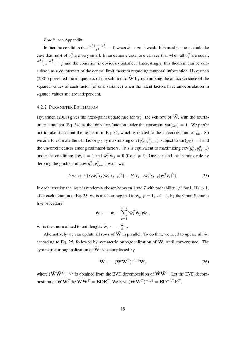
4.2.2 PARAMETER ESTIMATION
Hyvarinen (2001) gives the fixed-point update rule for wTi , the i-th row of W, with the fourth-
order cumulant (Eq. 34) as the objective function under the constraint var(yit) = 1. We prefer
not to take it account the last term in Eq. 34, which is related to the autocorrelation of yit. So
we aim to estimate the i-th factor yit by maximizing cov(y2it, y
2i,t−τ ), subject to var(yit) = 1 and
the uncorrelatedness among estimated factors. This is equivalent to maximizing cov(y2it, y
2i,t−τ )
under the conditions ||wi|| = 1 and wTi wj = 0 (for j 6= i). One can find the learning rule by
deriving the gradient of cov(y2it, y
2i,t−τ ) w.r.t. wi:
4wi ∝ E{εtwTi εt(wT
i εt−τ )2}+ E{εt−τ wTi εt−τ (wT
i εt)2}. (25)
In each iteration the lag τ is randomly chosen between 1 and 7 with probability 1/3 for 1. If i > 1,
after each iteration of Eq. 25, wi is made orthogonal to wp, p = 1, ...i− 1, by the Gram-Schmidt
like procedure:
wi ←− wi −i−1∑
p=1
(wTi wp)wp.
wi is then normalized to unit length: wi ←− wi||wi|| .
Alternatively we can update all rows of W in parallel. To do that, we need to update all wi
according to Eq. 25, followed by symmetric orthogonalization of W, until convergence. The
symmetric orthogonalization of W is accomplished by
W ←− (WWT )−1/2W. (26)
where (WWT )−1/2 is obtained from the EVD decomposition of WWT . Let the EVD decom-
position of WWT be WWT = EDET . We have (WWT )−1/2 = ED−1/2ET .
15

4.3 Conditional-Decorrelation GARCH Model
4.3.1 RATIONALE
In GO-GARCH it is assumed that the factors yit are conditionally uncorrelated such that the
conditional covariance matrix of yt is diagonal (see Eq. 16). But we just explicitly enforce
unconditional uncorrelatedness between factors, and certainly unconditional uncorrelatedness can
not guarantee conditional uncorrelatedness. It may cause large error in the estimated covariance
matrix if we simply regard unconditional uncorrelatedness as conditional uncorrelatedness. In
order to reduce the error in modelling the conditional covariance matrix, it is very natural to
enforce conditional decorrelation between factors.
In Matsuoka et al. (1995) it was shown that if the latent factors are conditionally uncorrelated
and their local variances fluctuate somewhat independently of each other,vii the factors (and the
matrix W) can be determined uniquely except for the trivial scaling and permutation indetermi-
nacies by making yit conditionally uncorrelated. So one can estimate the factors by enforcing
conditional decorrelation between factors.
4.3.2 PARAMETER ESTIMATION
Matsuoka et al. (1995) gave an algorithm to estimate yit and W by achieving conditional decor-
relation between yit. A simpler version was given in Hyvarinen et al., 2001, chap. 18. But
in these algorithms, we need to re-calculate the local covariances of factors after each iteration,
which causes high computational load.
In fact, in order to achieve conditional uncorrelatedness between factors, after whitening of
the data, the orthogonal matrix W should make all local covariance matrices of the whitened re-
turn series jointly as diagonal as possible. Therefore, after estimating a series of local covariance
matrices, W can be estimated by applying simultaneous diagonalization to these matrices. In
our experiments, we adopt this method. We use the simultaneous diagonalization method given
in Cardoso and Souloumiac (1996), and the local covariance is estimated using the exponentially
weighted moving average (EWMA) with the smoothing constant λ = 0.90.
vii. Mathematically speaking, the condition, which states that the local variances fluctuate some-
what independently of each other, means that for every pair of the factors, the ratio of their
local variances is not constant over time.
16

4.3.3 REMARK
It should be mentioned that recently, an approach for modelling multivariate volatilities via con-
ditional uncorrelated components (CUC’s) was proposed by Fan et al. (2005). The CUC’s in
their approach are actually the same as the conditionally uncorrelated factors in our CD-GARCH
model. In addition, as they exploit the extended GARCH model, which has a more general setting
than conventional GARCH, to model the volatility of each CUC, their approach is more flexible
than CD-GARCH. The consistency of the estimate of W is also proved in their work. In this
paper we discuss CD-GARCH from a different viewpoint. It is proposed as one of the simple
factor GARCH models and compared to others extensively. Moreover, in order to improve the
model flexibility, one can combine the factor model with the DCC model, as shown in Section 5.
4.4 Discussion
Now we give a summary and comments on the models proposed above. The three models use
different criteria to find the factors and W. Under some conditions, we can unify these models.
In fact, Independent-factor GARCH, best-factor GARCH, and conditional-decorrelation GARCH
give the same result if the following conditions are satisfied:
1. The factors yit are statistically independent of each other.
2. At most one of yit is normally distributed.
3. All yit have autocorrelation in their squared values and are temporally uncorrelated.
4. For every pair of yit, the ratio of their local variances is not constant over time.
Under the above conditions, each of the three models can give a unique result for the factors
(except for the permutation and scaling arbitrariness of the outputs), which is an estimate of the
latent factors generating the return series. Therefore the estimated factors and the matrix W must
be the same for the three models (with permutation indeterminacy ignored).
We should emphasize that in practice the above conditions may not exactly hold. Conse-
quently, these models may produce different estimates for W, since they focus on information of
different aspects and exploit different objective functions. The choice of the model depends on
which criterion is most consistent with the characteristics of financial data. We know that finan-
cial return series exhibit the volatility clustering phenomenon and their covariances change over
time. In order to capture the nonlinear dependency between outputs, ICA algorithms use higher-
order statistics explicitly or implicitly, which may be sensitive to the chosen data period of the
17

IF-GARCH BF-GARCH CD-GARCH
Criterion for
estimating
factors
Factors are statistically
as independent as possi-
ble (at most one factor is
normal.)
Each factor has the
largest autocorrelation in
squared values
Factors are conditionally
as uncorrelated as possi-
ble
Estimation
procedure
ICA (FastICA given
by Hyvarinen and Oja
(1997) is used) for
estimating W; Eq. 18
for constructing Ht
Eq. 25 for estimating W;
Eq. 18 for constructing
Ht
Simultaneous diago-
nalization (Cardoso &
Souloumiac, 1996) for
estimating W; Eq. 18
for constructing Ht
Computation involve low computation
Remark provide the same result under certain conditions
Table 1: Summary of the three multivariate factor GARCH models.
nonstationary financial data and outliers. This may cause a problem in constructing independent
factor models in finance. Autocorrelation in squared values of a series is also sensitive to out-
liers (Alexander, 2001, chap. 4), so the result of BF-GARCH may also be sensitive to outliers. In
CD-GARCH, we do not exploit the information regarding the distributions of the factors. We just
utilize the second-order statistics averaged for all time instants. Hence it should be more robust
to outliers. Also recall that GO-GARCH explicitly assumes that the factors are conditionally un-
correlated. We therefore conjecture that CD-GARCH should describe the multivariate financial
return series best.
All these three models are estimated easily, and the estimation involves low computation. In
particular, IF-GARCH and CD-GARCH (based on simultaneous diagonalization of local covari-
ances) are computationally very efficient. Note that in the estimation of BF-GARCH, in each
iteration of the learning rule Eq. 25, the time lag τ is randomly chosen, which may slower the
convergence a little. Table 1 summarizes the characteristics of these models. The behavior of
these models will be experimentally studied in Section 7.
In Section 3.3 we claimed that one can use PCA as preprocessing to reduce the number of
factors. In fact, even if we don’t use PCA, it is still possible to reduce the number of factors,
by analyzing the estimated A. Denote the i-th cloumn of A by ai. Clearly ||ai||2 indicates the
total variance that the i-th factor contributes to all return series. We can reduce the number of
factors according to the order of ||ai||2. As a consequence, large covariance matrices can be
18

approximately generated by only a small number of factors. If necessary, one may resort to other
more complex criteria to determine the number of factors. For instance, Chan and Cha (2001)
exploited the minimum description length (MDL) principle to do that.
5. Factor-DCC Model: Factor Model coupled with DCC
5.1 The DCC Model
The DCC model, given by Engle (2002), is a generalization of CCC model (Bollerslev, 1990).
The CCC model assumes that the time-varying of conditional covariances is caused by the time-
varying of the conditional variance of each return series:
Ht = DtRDt, (27)
where Dt = diag{√hit} and hit denotes the conditional variance of the i-th return.
The DCC model differs only in allowing R to be time-varying:
Ht = DtRtDt. (28)
The conditional correlation matrix Rt is determined by another matrix Qt, which is used to model
the dynamic correlation structure of the standardized residual zt by the univariate GARCH(1,1)
formulation:
Qt = (1− α− β)Q + αzt−1zTt−1 + βQt−1, (29)
where Q is the unconditional covariance matrix of zt. The (i, j)-th entry of the conditional
correlation matrix Rt, denoted by ρi,j,t, is estimated as
ρi,j,t =qi,j,t√
qi,i,tqj,j,t, (30)
where qi,j,t is the (i, j)-th entry of Qt.
5.2 Why is DCC Embedded?
van der Weide (2002) demonstrated that GO-GARCH produces time-varying conditional correla-
tion and that the conditional correlation is bounded. In practice, factor GARCH models may not
fully capture the dynamic behavior of the conditional correlation of return series. Consequently,
the factors may still have some remaining conditional correlation.
In order to model Ht more accurately, we no longer treat Σt as a diagonal matrix, as shown
in Eq. 16, but model it with the DCC model. In this way the factor-DCC model is constructed,
as an extension of the corresponding factor-GARCH model. Clearly DCC would provide a better
19

estimate for Σt than the diagonal matrix, and as a consequence, the capacity of factor GARCH
is extended by embedding DCC for modelling the conditional correlations between factors. In
other words, the factor-DCC model should have better flexibility than the corresponding factor
GARCH model. On the other hand, the performance of the extended model is also better than
that of DCC, as explained below.
In the factor GARCH models we proposed, the factors are estimated very conveniently such
that the recovery of factors can even be considered as a preprocessing step. After this step, the
factors are expected to exhibit the following features.
• The conditional correlation matrix of yt is close to the identity matrix and its variability is
greatly reduced. This is because the factors (especially those extracted in IF-GARCH and
CD-GARCH) are approximately conditionally uncorrelated.
• Compared to the original return series, the factors (especially those obtained in BF-GARCH)
would exhibit higher autocorrelation in squared values and can be modeled better with uni-
variate GARCH models.
According to these features, Σt should be modeled better by the DCC model (Engle, 2002) than
Ht. In other words, the performance of DCC is improved by incorporating the linear transforma-
tion stage W.
5.3 Factor-DCC Model
Now we adopt the DCC model to describe the conditional covariance matrix between factors, i.e.
Σt = DtRtDt, (31)
where Dt = diag{√hyit} and Rt denotes the conditional correlation matrix of yt. Rt is given
by Eq. 29 and Eq. 30. The conditional covariance matrix of return series is given by Eq. 18. The
structure of the factor-DCC is illustrated in Figure 1.
The factor-DCC model represents the conditional covariance matrix of the whitened data εt
as Ht = WTDtRtDtW. The quasi log-likelihood for εt is
lT = −12
T∑
t=1
[m log(2π) + log |Ht|+ εTt H−1
t εt]
= −12
T∑
t=1
{[m log(2π) +
m∑
i=1
(log hyit + z2
it
)]
+[log |Rt|+ zT
t R−1t zt − zT
t zt
]}.
20
DCC...W Σt
Factor extraction DCC for modeling the conditional covariance matrix of factors
.
.
.
y
y
1t
mt
1t
nt
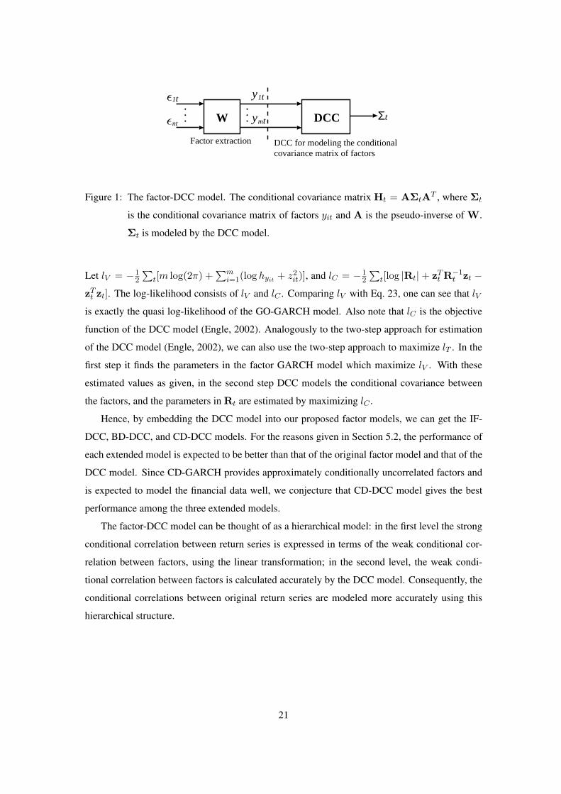
Figure 1: The factor-DCC model. The conditional covariance matrix Ht = AΣtAT , where Σt
is the conditional covariance matrix of factors yit and A is the pseudo-inverse of W.
Σt is modeled by the DCC model.
Let lV = −12
∑t[m log(2π) +
∑mi=1(log hyit + z2
it)], and lC = −12
∑t[log |Rt| + zT
t R−1t zt −
zTt zt]. The log-likelihood consists of lV and lC . Comparing lV with Eq. 23, one can see that lV
is exactly the quasi log-likelihood of the GO-GARCH model. Also note that lC is the objective
function of the DCC model (Engle, 2002). Analogously to the two-step approach for estimation
of the DCC model (Engle, 2002), we can also use the two-step approach to maximize lT . In the
first step it finds the parameters in the factor GARCH model which maximize lV . With these
estimated values as given, in the second step DCC models the conditional covariance between
the factors, and the parameters in Rt are estimated by maximizing lC .
Hence, by embedding the DCC model into our proposed factor models, we can get the IF-
DCC, BD-DCC, and CD-DCC models. For the reasons given in Section 5.2, the performance of
each extended model is expected to be better than that of the original factor model and that of the
DCC model. Since CD-GARCH provides approximately conditionally uncorrelated factors and
is expected to model the financial data well, we conjecture that CD-DCC model gives the best
performance among the three extended models.
The factor-DCC model can be thought of as a hierarchical model: in the first level the strong
conditional correlation between return series is expressed in terms of the weak conditional cor-
relation between factors, using the linear transformation; in the second level, the weak condi-
tional correlation between factors is calculated accurately by the DCC model. Consequently, the
conditional correlations between original return series are modeled more accurately using this
hierarchical structure.
21

Stock Mean Std. Skewness Excess
kurtosis
First-order
autocorrela-
tion coeff.
in squared
returns
Box-Pierce
LM (Lag
p=5)
CHEUNG KONG
(0001.HK)
0.00071 0.0223 0.644 7.92 0.165 48.13∗
CLP HOLDINGS
(0002.HK)
0.00052 0.0161 0.729 12.17 0.245 17.89∗
HK & CHINA GAS
(0003.HK)
0.00063 0.0178 0.388 7.47 0.233 28.64∗
HSBC HOLDINGS
(0005.HK)
0.00091 0.0176 0.337 11.90 0.390 24.75∗
HK ELECTRIC
(0006.HK)
0.00052 0.0162 0.212 9.66 0.327 25.49∗
HANG LUNG
GROUP (0010.HK)
0.00047 0.0214 0.161 5.98 0.191 1.26
HANG SENG BANK
(0011.HK)
0.00081 0.0190 0.160 7.33 0.368 27.02∗
HENDERSON LAND
(0012.HK)
0.00073 0.0243 0.558 5.50 0.189 26.02∗
HUTCHISON
(0013.HK)
−0.00073 0.0226 0.498 6.91 0.222 25.11∗
CATHAY PAC AIR
(0293.HK)
0.00043 0.0240 0.168 5.38 0.128 18.53∗
∗ Significant at 1% level.
Table 2: Return series used in the experiment and their statistics.
6. Experiment with Real Data: Empirical Study
In the experiment, 10 stock returns selected from the Hang Seng Index constitutes in the Hong
Kong stock market are used. We use the daily dividend/split adjusted closing prices started from
June 22th, 1990 to April 9th, 2004. Denoting the closing price by Pt, the return is calculated as
rt =Pt − Pt−1
Pt−1(32)
Each return series contains 3600 observations. For the few days when the price is not available,
we use the simple linear interpolation to estimate the price. Table 2 gives some statistics of
the daily returns of these stocks. From this table, we can see clearly that most stocks have the
GARCH effect.
Here we compare 10 multivariate GARCH models, which are the O-GARCH (Alexander,
2000), DCC model (Engle, 2002), GO-GARCH with QML (van der Weide, 2002), IF-GARCH,
BF-GARCH, CD-GARCH, and the factor-DCC models GO-DCC (GO-GARCH coupled with
22

DCC), IF-DCC, BF-DCC, CD-DCC. The DCC model is chosen for comparison for two reasons.
First, other basic models, such as the the vech model (Bollerslev et al., 1988) and the BEKK
model (Engle & Kroner, 1995), have too many parameters and thus are not suitable for modelling
the conditional covariance matrix of high dimension. Second, the DCC model is a popular one
and has been shown to perform well in a number of situations (Engle, 2002). All experiments
in this paper are conducted using MATLAB. For the estimation of DCC, O-GARCH, and the
univariate GARCH model, we use the UCSD GARCH toolbox developed by Sheppard (2002). In
the estimation of GO-GARCH, we use the MATLAB nonlinear constrained optimization toolbox
to optimize the QML. Other MATLAB source codes used in experiments are available from
http://www.cse.cuhk.edu.hk/∼kzhang/factor garch.
We use 3000 points from all 3600 observations for training, and the other 600 are used for
testing. We use two measures to evaluate the forecasting performance of these models. They are
(log-)QML and the Value-at-Risk (VaR) performance. The (log-)QML has been used to evaluate
the performance of GARCH models in Bollerslev et al. (1994):
QML =T∑
t=1
log G(εt;0,Ht)
= −12
T∑
t=1
[n log(2π) + log |Ht|+ εTt H−1
t εt].
We use the QML, rather than the true likelihood, because it is hard to specify the true conditional
distribution of returns and the QML provides an approximate for the true maximum likelihood.
Note that in Section. 3.3, we have shown the relationship between the likelihood attained and the
statistical dependence in standardized residuals. For some given multivariate return series, the
larger the likelihood function, the more independent the standardized residuals.
To save space, the estimated parameters for modelling the conditional covariance matrix of
the 10 stocks are not reported here, as the number of parameters is too large. Later we will give
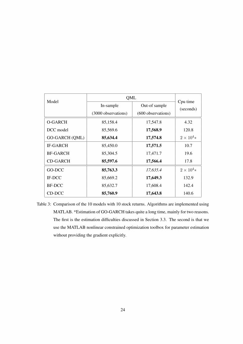
the estimated parameter values together with the standard errors for 5-dimensional data. Table 3
presents the in-sample and out-of-sample QML values. Note that of course GO-GARCH by
maximizing QML gives the highest in-sample QML among the factor models, since it explicitly
maximizes the quasi likelihood. But it does not necessarily maximize the true likelihood. As we
care about the generalization behavior of the models, we would evaluate the GARCH models by
comparing their out-of-sample QML.
Among the first six GARCH models, GO-GARCH, CD-GARCH, IF-GARCH, and DCC give
similar performance. If we take into account of the computational load, obviously CD-GARCH
and IF-GARCH are plausible. Among the factor-DCC models, the CD-DCC model performs
23
ModelQML
Cpu timeIn-sample
(3000 observations)
Out-of sample
(600 observations)(seconds)
O-GARCH 85,158.4 17,547.8 4.32
DCC model 85,569.6 17,568.9 120.8
GO-GARCH (QML) 85,634.4 17,574.8 2× 10⁴∗IF-GARCH 85,450.0 17,571.5 10.7
BF-GARCH 85,304.5 17,471.7 19.6
CD-GARCH 85,597.6 17,566.4 17.8
GO-DCC 85,763.3 17,635.4 2× 10⁴∗IF-DCC 85,669.2 17,649.3 132.9
BF-DCC 85,632.7 17,608.4 142.4
CD-DCC 85,760.9 17,643.8 140.6
Table 3: Comparison of the 10 models with 10 stock returns. Algorithms are implemented using
MATLAB. *Estimation of GO-GARCH takes quite a long time, mainly for two reasons.
The first is the estimation difficulties discussed in Section 3.3. The second is that we
use the MATLAB nonlinear constrained optimization toolbox for parameter estimation
without providing the gradient explicitly.
24

the best, with IF-DCC close behind. Each factor-DCC model gives better performance than
the corresponding factor model as well as the DCC model. We can see that by incorporating
the factor extraction procedure, the performance of DCC is greatly improved, with only slight
increase in computational time. This also verifies the usefulness of factor models for constructing
multivariate GARCH models. Note that the difference in QML for different models is not very
large, since the quasi likelihood function is almost flat in the neighborhood of its optimum (Jerez
et al., 2000).
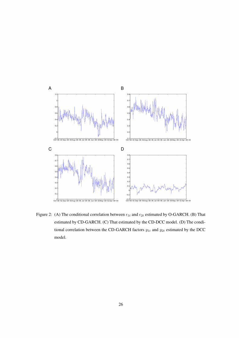
Figure 2 shows the conditional correlation between the first and second return series esti-
mated by O-GARCH, CD-GARCH, and the CD-DCC model, respectively. We can see that the
conditional correlation estimated by CD-GARCH (Figure 2B) and that estimated by the CD-DCC
model (Figure 2C) are very similar. Their trend lies in a lower level after November, 1999, while
the result obtained by O-GARCH does not (Figure 2A). The conditional correlation between the
CD-GARCH factors y1t and y2t estimated by the DCC model is also given in Figure 2 (D), from
which we can see the correlation between y1t and y2t is comparatively small and oscillates around
0, which agree with our claims in Section 5.2.
In order to reduce the random effect and to compare these models more convincingly, we
conduct five more experiments. In each experiment we randomly select five stocks from all of
the 10 stocks used in the first experiment. Table 4 lists the parameter values estimated in the first
experiment with five stocks. The standard errors are given in the parentheses. They are computed
by the bootstrapping method described in Fan et al. (2005) (with 200 replications).viii We use the
Amari performance index Perr (Cichocki & Amari, 2003) to measure the distance between two
matrices W1 and W2. Let pij = [W1W−12 ]ij . Perr is defined as
Perr =1
m(m− 1)
m∑
i=1
{( m∑
j=1
|pij |maxk |pik| − 1
)+
( m∑
j=1
|pji|maxk |pki| − 1
)}. (33)
Particularly, this performance index measures how close W1W−12 is to the generalized permu-
tation matrix. The smaller Perr is, the closer W1W−12 is to the generalized permutation matrix.
Permutation and scaling of row of W1 and W2 do not affect this measure. From the parameter
viii. Fan et al. (2005) gave the bootstrapping procedure for computing standard errors (or confi-
dence sets) of the parameters in factor GARCH models. For DCC and factor-DCC models,
the procedure is quite similar. In the bootstrap sampling procedure, we just need to obtain
the standardized residuals as H−1/2t εt, to draw the standardized residuals by sampling with
replacement, and to generate new observations according to the multivariate GARCH model
under study with the estimated parameters.
25
A
Oct−08−92 Sep−08−94Aug−08−96 Jul−09−98 Jun−08−00May−09−02Apr−08−04−0.2
0
0.2
0.4
0.6
0.8
1
1.2
B
Oct−08−92 Sep−08−94Aug−08−96 Jul−09−98 Jun−08−00May−09−02Apr−08−040.1
0.2
0.3
0.4
0.5
0.6
0.7
0.8
C
Oct−08−92 Sep−08−94Aug−08−96 Jul−09−98 Jun−08−00May−09−02Apr−08−040
0.1
0.2
0.3
0.4
0.5
0.6
0.7
0.8
D
Oct−08−92 Sep−08−94Aug−08−96 Jul−09−98 Jun−08−00May−09−02Apr−08−04−0.2
−0.1
0
0.1
0.2
0.3
0.4
0.5
0.6
0.7
0.8
Figure 2: (A) The conditional correlation between ε1t and ε2t estimated by O-GARCH. (B) That
estimated by CD-GARCH. (C) That estimated by the CD-DCC model. (D) The condi-
tional correlation between the CD-GARCH factors y1t and y2t estimated by the DCC
model.
26

values in Table 4, one can see that some factors may be fitted better by an integrated GARCH
model. Table 5 gives the distance among W in different models. We can see that W in CD-
GARCH is close to that in GO-GARCH and IF-GARCH, meaning that the criteria for factor
extraction in these three models are consistent to a certain extent.
Table 6 shows the in-sample and out-of-sample QML for these five experiments. When
summed over all five cases, we can see clearly that among the factor GARCH models and the
DCC model, CD-GARCH and DCC are the best, and IF-GARCH is very close behind. For the
factor-DCC models, the CD-DCC model always performs best, followed by the IF-DCC model.
Note that the independent factor model is estimated very fast, so IF-GARCH and IF-DCC give
comparatively good results with low computation.
Now let us compare these models by investigating the forecasting performance of the 5%
VaR for portfolios with fixed weights. We consider an equally weighted portfolio and a hedge
portfolio. For constructing the hedge portfolio of 10 stocks, the weight for the first five stocks
is 0.2 and that for the others is -0.2. The weight vector for the hedge portfolio consisting of five
stocks is (0.5, 0.5,−0.3,−0.3,−0.4)T . In calculation of the VaR, the standardized residuals are
assumed to follow the normal distribution.
27

Mod
elD
CC
GO
-GA
RC
HG
O-D
CC
IF-G
AR
CH
IF-D
CC
BF-
GA
RC
HB
F-D
CC
CD
-GA
RC
HC
D-D
CC
W—
*(P
err
:0.0
190)
**(P
err
:0.0
262)
***
(Perr
:0.0
661)
****
(Perr
:0.0
245)
α1
0.11
86(0
.010
2)0.
0544
(0.0
084)
0.07
99(0
.010
3)0.
0905
(0.0
118)
0.06
59(0
.010
8)
β1
0.88
09(0
.010
5)0.
9379
(0.0
106)
0.90
93(0
.011
8)0.
9004
(0.0
135)
0.92
53(0
.013
2)
α2
0.08
51(0
.011
1)0.
0437
(0.0
073)
0.03
12(0
.008
3)0.
0293
(0.0
038)
0.02
94(0
.005
5)
β2
0.89
42(0
.016
2)0.
9513
(0.0
094)
0.96
39(0
.012
5)0.
9673
(0.0
047)
0.96
65(0
.007
5)
α3
0.12
20(0
.016
6)0.
0548
(0.0
047)
0.07
37(0
.011
4)0.
0580
(0.0
090)
0.08
41(0
.011
8)
β3
0.87
22(0
.017
7)0.
9397
(0.0
052)
0.91
61(0
.014
0)0.
9303
(0.0
125)
0.90
79(0
.012
2)
α4
0.09
94(0
.009
5)0.
0277
(0.0
042)
0.05
49(0
.006
9)0.
0424
(0.0
046)
0.05
47(0
.005
0)
β4
0.89
02(0
.010
1)0.
9691
(0.0
059)
0.93
60(0
.009
2)0.
9529
(0.0
057)
0.93
94(0
.005
6)
α5
0.08
74(0
.006
2)0.
0902
(0.0
093)
0.05
01(0
.000
1)0.
0493
(0.0
091)
0.04
23(0
.006
4)
β5
0.89
73(0
.008
5)0.
9030
(0.0
100)
0.94
99(0
.000
1)0.
9416
(0.0
126)
0.95
30(0
.008
1)
αD
CC
0.01
30(0
.000
8)—
0.01
01(0
.001
1)—
0.01
29(0
.000
8)—
0.01
18(0
.001
4)—
0.01
13(0
.000
9)
βD
CC
0.98
29(0
.000
14)
—0.
9729
(0.0
045)
—0.
9799
(0.0
022)
—0.
9805
(0.0
033)
—0.
9748
(0.0
028)
∗WG
O=
−63.1
309
−1.3
950
70.6
358
−3.9
647
4.9
817
−7.6
802
−1.9
740
5.8
658
71.4
124
−74.8
239
27.1
660
13.1
141
21.5
107
−33.2
691
−25.6
074
−20.3
211
55.6
060
−14.3
885
2.3
388
−17.4
138
36.8
576
6.8
855
23.1
277
7.4
234
−4.8
296
.∗∗
WIF
=
−69.0
825
2.6
734
13.2
643
−8.0
793
8.5
702
9.2
869
−56.3
526
12.2
650
−0.5
828
16.7
259
−32.6
966
−0.9
289
73.2
649
−0.6
530
3.1
127
−12.8
686
−9.6
418
−22.2
190
−9.9
944
61.3
561
−21.4
619
−6.3
775
−6.3
761
78.2
108
−49.7
823
.
∗∗∗W
BF
=
20.6
899
8.3
840
30.3
021
13.3
088
−3.9
912
22.8
921
−39.1
274
26.5
732
21.4
409
−32.8
858
−70.7
030
8.6
297
59.5
367
16.2
540
−20.1
137
−23.9
947
−33.0
844
−14.6
084
38.2
933
20.4
068
5.2
096
23.3
872
−29.0
875
62.5
736
−68.4
641
.∗∗
∗∗W
CD
=
41.0
158
1.3
977
−75.2
921
3.5
068
−4.4
484
−19.6
151
53.9
973
−13.2
330
2.8
600
−9.9
846
61.9
166
2.0
958
−4.8
322
6.7
886
−6.0
013
−23.2
127
−19.8
721
−17.9
987
30.4
136
30.0
664
10.6
948
−0.5
534
−6.0
945
−72.7
414
74.4
732
. Tabl
e4:
Est
imat
eof
the
para
met
ers
indi
ffer
entm
odel
sfo
raco
mbi
natio
nof
five
retu
rnse
ries
.Num
bers
inth
epa
rent
hese
sar
eth
est
anda
rder
rors
.
Inth
eD
CC
mod
el,α
ian
dβ
iar
eG
AR
CH
para
met
ers
for
the
retu
rnse
ries
,whi
lein
othe
rm
odel
s,th
eyar
eG
AR
CH
para
met
ers
for
the
fact
ors.
28

WGO WIF WBF WCD
WGO
WIF 0.3531
WBF 0.4192 0.8347
WCD 0.1818 0.2326 0.5447
Table 5: The distance among WGO, WIF , WBF , and WCD, measured by the Amari perfor-
mance index Perr.
Two statistical tests are used to evaluate the VaR forecasting performance. They are the
Dynamic quantile (DQ) test by Engle and Manganelli (2004) and the Kupiec LR test given in Ku-
piec (1995). The DQ test examines the independence of a HIT from past HITs, from the predicted
VaR, or from any other variables, and HIT is defined as I(rt < VaRα) − α, where α is the VaR
level. In our experiments, we use five lags for past HITs and the current VaR. The Kupiec LR
test compares the empirical failure rate to its theoretical value. Tables 7 and 8 summarize the
in-sample VaR0.05 violations and the statistical test results, and Tables 9 and 10 give the out-
of-sample results. The models are compared in terms of the number of rejections at 1% or 5%
significant level.
One should be aware that the evaluation of GARCH models by examining the VaRs of a
set of given portfolios may not be very reliable. Engle and Manganelli (2004) claimed that al-
though GARCH might be useful for describing the evolution of volatility, it might provide an
unsatisfactory approximation when applied to tail estimation. Moreover, the sensitivity of the
VaR failure rates with respect to the distributional assumptions is found to be larger than that
with respect to the parametric specification for the multivariate GARCH models (Rombouts &
Verbeek, 2004).ix However, when summed over all the cases, we can see that factor-DCC mod-
els give the best VaR0.05 prediction performance. And among the factor GARCH models, the
result of O-GARCH is not as good as that of others. These findings are especially obvious in the
out-of-sample case.
ix. Rombouts and Verbeek (2004) also proposed a semi-parametric model for the distribution of
the standardized residuals and found that it can improve the VaR forecasting performance.
However, this approach does not apply here since the data dimension is high.
29

Mod
elQ
ML
Exp
1E
xp2
Exp
3E
xp4
Exp
5
O-G
AR
CH
In-s
ampl
e39
,852
.0(-
177.
6)42
,360
.7(-
343.
9)40
,944
.4(-
271.
8)40
,216
.0(-
132.
6)41
,140
.4(-
568.
7)
Out
-of-
sam
ple
8,62
2.9
(-13
.1)
8,74
7.6
(-23
.3)
8,62
6.2
(0)
8,47
6.3
(-2.
6)8,
742.
9(-
42.3
)
DC
Cm
odel
In-s
ampl
e40
,029
.6(0
)42
,675
.2(-
29.4
)41
,216
.2(0
)40
,342
.9(-
5.7)
41,7
09.1
(0)
Out
-of-
sam
ple
8,63
6.0
(0)
8,75
9.7
(-11
.2)
8,62
3.3
(-2.
9)8,
476.
7(-
2.2)
8,76
8.1
(-17
.1)
GO
-GA
RC
HIn
-sam
ple
40,0
26.1
(-3.
5)42
,704
.6(0
)41
,185
.8(-
30.4
)40
,348
.6(0
)41
,708
.1(-
1.0)
Out
-of-
sam
ple
8,61
6.9
(-19
.1)
8,74
8.5
(-22
.4)
8,59
4.8
(-31
.4)
8,44
3.7
(-35
.2)
8,75
9.8
(-25
.4)
IF-G
AR
CH
In-s
ampl
e39
,980
.7(-
48.9
)42
,564
.7(-
139.
9)41
,100
.1(-
116.
1)40
,254
.8(-
93.8
)41
,602
.1(-
107.
0)
Out
-of-
sam
ple
8,63
2.2
(-3.
8)8,
757.
8(-
13.1
)8,
620.
5(-
5.7)
8,47
8.9
(0)
8,78
5.2
(0)
BF-
GA
RC
HIn
-sam
ple
39,9
76.5
(-53
.1)
42,5
86.4
(-11
8.2)
40,9
87.0
(-22
9.2)
40,3
30.9
(-17
.7)
41,5
03.8
(-20
5.3)
Out
-of-
sam
ple
8,61
8.9
(-17
.1)
8,75
7.4
(-13
.5)
8,56
1.7
(-64
.5)
8,47
2.3
(-6.
6)8,
730.
6(-
54.6
)
CD
-GA
RC
HIn
-sam
ple
39,9
88.3
(-41
.3)
42,6
47.5
(-57
.1)
41,1
45.9
(-70
.3)
40,2
92.8
(-55
.8)
41,6
87.5
(-21
.6)
Out
-of-
sam
ple
8,62
5.8
(-10
.2)
8,77
0.9
(0)
8,62
3.6
(-2.
6)8,
476.
3(-
2.6)
8,76
9.9
(-15
.3)
GO
-DC
CIn
-sam
ple
40,0
96.0
(0)
42,7
70.6
(0)
41,2
56.1
(0)
40,3
74.7
(-2.
4)41
,801
.2(0
)
Out
-of-
sam
ple
8,64
9.9
(-7.
1)8,
788.
9(-
9.3)
8,64
1.3
(-11
.9)
8,47
5.4
(-25
.1)
8,80
1.3
(-5.
5)
IF-D
CC
In-s
ampl
e40
,075
.0(-
21.0
)42
,705
.2(-
65.4
)41
,241
.6(-
14.5
)40
,363
.1(-
14.0
)41
,764
.5(-
36.7
)
Out
-of-
sam
ple
8,65
7.0
(0)
8,79
1.3
(-6.
9)8,
649.
6(-
3.6)
8,50
0.5
(0)
8,80
6.8
(0)
BF-
DC
CIn
-sam
ple
40,0
53.4
(-42
.6)
42,7
40.6
(-30
.0)
41,1
91.6
(-64
.5)
40,3
76.7
(-0.
4)41
,734
.0(-
67.2
)
Out
-of-
sam
ple
8,65
3.8
(-3.
2)8,
798.
2(0
)8,
629.
1(-
24.1
)8,
498.
4(-
2.1)
8,79
0.5
(-16
.3)
CD
-DC
CIn
-sam
ple
40,0
70.8
(-25
.2)
42,7
48.5
(-22
.1)
41,2
51.1
(-5.
0)40
,377
.1(0
)41
,793
.1(-
8.1)
Out
-of-
sam
ple
8,65
4.0
(-3.
0)8,
797.
0(-
1.2)
8,65
3.2
(0)
8,49
9.6
(-0.
9)8,
803.
5(-
3.3)
Tabl
e6:
Qua
silik
elih
ood
ofth
e10
mod
elsm
odel
ling
the
cond
ition
alco
vari
ance
offiv
ere
turn
seri
es.T
henu
mbe
rin
the
pare
nthe
sesi
sthe
diff
eren
ce
betw
een
the
corr
espo
ndin
gva
lue
and
the
larg
estv
alue
inth
atgr
oup.
Gro
up1
incl
udes
the
first
six
mod
els,
and
the
othe
rm
odel
sar
ein
grou
p2.
30

O-G
AR
CH
DC
CG
O-G
AR
CH
IF-G
AR
CH
BF-
GA
RC
HC
D-G
AR
CH
GO
-DC
CIF
-DC
CB
F-D
CC
CD
-DC
C
With
10st
ocks
%of
HIT
s5.
004.
404.
8345
.00
4.87
4.60
5.07
4.87
5.17
5.00
DQ
test
(p-v
alue
)0.
0180
0.10
470.
238
0.05
410.
0009
0.17
850.
3902
0.14
360.
3037
0.37
69
Kup
iec
test
(p-v
alue
)1
0.12
40.
6737
0.20
150.
7365
0.30
850.
8672
0.73
650.
6769
1
Exp
1w
ith5
stoc
ks
%of
HIT
s4.
534.
474.
604.
474.
374.
474.
374.
404.
274.
20
DQ
test
(p-v
alue
)0.
8330
0.83
020.
6919
0.86
170.
6390
0.86
870.
4305
0.50
070.
4188
0.32
80
Kup
iec
test
(p-v
alue
)0.
2337
0.17
260.
3085
0.17
260.
1041
0.17
260.
1041
0.12
400.
0590
0.03
89
Exp
2w
ith5
stoc
ks
%of
HIT
s4.
674.
375.
034.
635.
335.
234.
934.
534.
805.
03
DQ
test
(p-v
alue
)0.
0120
0.00
150.
0576
0.00
780.
0552
0.02
100.
0363
0.00
160.
0975
0.00
51
Kup
iec
test
(p-v
alue
)0.
3971
0.10
410.
9333
0.35
110.
4070
0.56
050.
8667
0.23
370.
6130
0.93
33
Exp
3w
ith5
stoc
ks
%of
HIT
s4.
774.
674.
934.
874.
774.
804.
974.
674.
834.
97
DQ
test
(p-v
alue
)0.
8590
0.79
410.
2424
0.67
450.
7227
0.91
760.
2643
0.81
450.
8990
0.26
43
Kup
iec
test
(p-v
alue
)0.
5547
0.39
710.
8667
0.73
650.
5547
0.61
300.
9332
0.39
710.
6737
0.93
32
Exp
4w
ith5
stoc
ks
%of
HIT
s5.
374.
835.
505.
235.
375.
375.
005.
005.
275.
27
DQ
test
(p-v
alue
)0.
0054
0.02
080.
0007
0.02
640.
0008
0.00
090.
0069
0.06
050.
0116
0.00
30
Kup
iec
test
(p-v
alue
)0.
3622
0.67
370.
2159
0.56
050.
3622
0.36
221.
0000
1.00
000.
5063
0.50
63
Exp
5w
ith5
stoc
ks
%of
HIT
s4.
073.
604.
133.
904.
073.
834.
174.
134.
304.
17
DQ
test
(p-v
alue
)0.
2004
0.03
130.
5562
0.04
880.
6882
0.16
590.
1364
0.20
030.
2460
0.03
19
Kup
iec
test
(p-v
alue
)0.
0155
0.00
020.
0249
0.00
410.
0155
0.00
230.
0313
0.02
490.
0718
0.03
13
No.
ofre
ject
ions
at1%
leve
l
DQ
test
11
11
21
11
02
Kup
iec
test
01
01
01
00
00
No.
ofre
ject
ions
at5%
leve
l
DQ
test
33
13
22
21
13
Kup
iec
test
11
11
11
11
02
Not
e:C
oeffi
cien
tssi
gnifi
cant
at5%
(1%
)for
mat
ted
inita
lic(b
old)
.
Tabl
e7:
In-s
ampl
eV
aR0.0
5vi
olat
ions
and
p-v
alue
sof
the
stat
istic
alte
sts
fora
hedg
epo
rtfo
lio.
QR
test
deno
tes
the
dyna
mic
quan
tile
test
.Fo
rthe
port
folio
cons
istin
gof
10st
ocks
,the
wei
ghtf
orth
efis
tfive
stoc
ksis
0.2,
and
that
for
the
othe
rsis
-0.2
.Fo
rth
epo
rtfo
lioco
nsis
ting
of5
stoc
ks,t
hew
eigh
tvec
tori
s(0
.5,0
.5,−
0.3,−0
.3,−
0.4)
T.
31

O-G
AR
CH
DC
CG
O-G
AR
CH
IF-G
AR
CH
BF-
GA
RC
HC
D-G
AR
CH
GO
-DC
CIF
-DC
CB
F-D
CC
CD
-DC
C
With
10st
ocks
%of
HIT
s5.
074.
204.
633.
474.
403.
634.
874.
434.
434.
30
DQ
test
(p-v
alue
)0.
0951
0.02
180.
0028
00.
0010
00.
0017
0.00
090.
0017
0.00
01
Kup
iec
LR
test
(p-v
alue
)0.
8672
0.03
890.
3511
00.
124
0.00
030.
7365
0.14
680.
1468
0.07
18
Exp
1w
ith5
stoc
ks
%of
HIT
s4.
004.
834.
534.
174.
474.
074.
704.
774.
674.
63
DQ
test
(p-v
alue
)0.
0000
0.12
790.
0085
0.02
470.
0060
0.00
480.
0060
0.00
970.
0032
0.02
86
Kup
iec
LR
test
(p-v
alue
)0.
0093
0.67
370.
2337
0.03
130.
1726
0.01
550.
4465
0.55
470.
3971
0.35
11
Exp
2w
ith5
stoc
ks
%of
HIT
s3.
604.
404.
673.
574.
773.
834.
674.
374.
574.
33
DQ
test
(p-v
alue
)0.
0000
0.07
070.
0085
0.00
030.
0650
0.00
090.
0240
0.01
170.
0172
0.00
60
Kup
iec
LR
test
(p-v
alue
)0.
0002
0.12
410.
3971
0.00
020.
5547
0.00
230.
3971
0.10
410.
2694
0.08
67
Exp
3w
ith5
stoc
ks
%of
HIT
s3.
974.
574.
603.
804.
703.
974.
534.
404.
504.
33
DQ
test
(p-v
alue
)0.
0000
0.00
870.
0092
0.00
000.
0433
0.00
010.
0071
0.00
080.
0171
0.00
04
Kup
iec
LR
test
(p-v
alue
)0.
0071
0.26
940.
3085
0.00
170.
4465
0.00
710.
2337
0.12
410.
2015
0.08
67
Exp
4w
ith5
stoc
ks
%of
HIT
s3.
674.
634.
173.
674.
933.
704.
434.
304.
974.
43
DQ
test
(p-v
alue
)0.
0000
0.67
190.
0002
0.00
000.
0869
0.00
000.
0048
0.00
010.
0867
0.00
23
Kup
iec
LR
test
(p-v
alue
)0.
0004
0.35
110.
0313
0.00
040.
8667
0.00
060.
1468
0.07
180.
9332
0.14
68
Exp
5w
ith5
stoc
ks
%of
HIT
s4.
004.
604.
674.
174.
804.
174.
834.
604.
804.
67
DQ
test
(p-v
alue
)0.
0000
0.07
580.
0197
0.00
030.
0467
0.00
100.
0474
0.01
240.
0906
0.03
60
Kup
iec
LR
test
(p-v
alue
)0.
0093
0.30
850.
3971
0.03
130.
6130
0.03
130.
6737
0.30
850.
6130
0.39
71
No.
ofre
ject
ions
at1%
leve
l
DQ
test
51
55
26
44
24
Kup
iec
test
50
04
04
00
00
No.
ofre
ject
ions
at5%
leve
l
DQ
test
52
66
46
66
46
Kup
iec
test
51
16
06
00
00
Not
e:C
oeffi
cien
tssi
gnifi
cant
at5%
(1%
)for
mat
ted
inita
lic(b
old)
.
Tabl
e8:
In-s
ampl
eV
aR0.0
5vi
olat
ions
and
corr
espo
ndin
gst
atis
tical
test
sfo
raeq
ually
wei
ghte
dpo
rtfo
lio.F
orth
epo
rtfo
lioco
nsis
ting
of10
stoc
ks,
the
wei
ghtf
orea
chst
ock
is0.
1.Fo
rthe
port
folio
cons
istin
gof
5st
ocks
,the
wei
ghtf
orea
chst
ock
is0.
2.
32

O-G
AR
CH
DC
CG
O-G
AR
CH
IF-G
AR
CH
BF-
GA
RC
HC
D-G
AR
CH
GO
-DC
CIF
-DC
CB
F-D
CC
CD
-DC
C
With
10st
ocks
%of
HIT
s4.
004.
334.
334.
003.
174.
174.
504.
334.
504.
33
DQ
test
(p-v
alue
)0.
7082
0.35
580.
7320
0.80
160.
2898
0.95
480.
7202
0.73
660.
5832
0.73
88
Kup
iec
test
(p-v
alue
)0.
2449
0.44
370.
4437
0.24
490.
0276
0.33
550.
5678
0.44
370.
5678
0.44
37
Exp
1w
ith5
stoc
ks
%of
HIT
s3.
004.
833.
833.
834.
174.
004.
674.
674.
674.
67
DQ
test
(p-v
alue
)0.
4044
0.87
270.
6036
0.61
080.
9435
0.89
120.
9635
0.99
030.
9900
0.99
04
Kup
iec
test
(p-v
alue
)0.
0155
0.85
060.
1722
0.17
220.
3355
0.24
490.
7049
0.70
490.
7049
0.70
49
Exp
2w
ith5
stoc
ks
%of
HIT
s2.
004.
332.
001.
831.
673.
004.
833.
833.
675.
17
DQ
test
(p-v
alue
)0.
0587
0.95
820.
0311
0.03
670.
0196
0.43
240.
9867
0.68
580.
6707
0.98
83
Kup
iec
test
(p-v
alue
)0.
0001
0.44
370.
0001
0.00
000.
0000
0.01
550.
8506
0.17
220.
1164
0.85
22
Exp
3w
ith5
stoc
ks
%of
HIT
s3.
673.
503.
673.
673.
674.
003.
333.
674.
003.
83
DQ
test
(p-v
alue
)0.
0333
0.00
070.
0334
0.03
280.
0337
0.00
730.
0095
0.03
200.
0074
0.00
37
Kup
iec
test
(p-v
alue
)0.
1164
0.07
540.
1164
0.11
640.
1164
0.24
490.
0467
0.11
640.
2449
0.17
22
Exp
4w
ith5
stoc
ks
%of
HIT
s5.
003.
675.
174.
673.
835.
173.
503.
332.
173.
83
DQ
test
(p-v
alue
)0.
9836
0.38
800.
9777
0.96
600.
8774
0.97
790.
5514
0.50
300.
4796
0.81
58
Kup
iec
test
(p-v
alue
)1.
0000
0.11
640.
8522
0.70
490.
1722
0.85
220.
0754
0.04
670.
0276
0.17
22
Exp
5w
ith5
stoc
ks
%of
HIT
s2.
002.
503.
002.
832.
173.
173.
673.
673.
833.
67
DQ
test
(p-v
alue
)0.
0047
0.04
180.
0775
0.04
410.
0122
0.12
220.
1446
0.14
810.
1635
0.14
37
Kup
iec
test
(p-v
alue
)0.
0001
0.00
190.
0155
0.00
820.
0004
0.02
760.
1164
0.11
640.
1722
0.11
64
No.
ofre
ject
ions
at1%
leve
l
DQ
test
11
00
01
10
11
Kup
iec
test
21
12
20
00
00
No.
ofre
ject
ions
at5%
leve
l
DQ
test
22
23
31
11
11
Kup
iec
test
31
22
32
11
10
Not
e:C
oeffi
cien
tssi
gnifi
cant
at5%
(1%
)for
mat
ted
inita
lic(b
old)
.
Tabl
e9:
Out
-of-
sam
ple
VaR
0.0
5vi
olat
ions
and
corr
espo
ndin
gst
atis
tical
test
sfo
ra
hedg
epo
rtfo
lio.
For
the
port
folio
cons
istin
gof
10st
ocks
,
the
wei
ght
for
the
fist
five
stoc
ksis
0.2,
and
that
for
the
othe
rsis
-0.2
.Fo
rth
epo
rtfo
lioco
nsis
ting
of5
stoc
ks,
the
wei
ght
vect
oris
(0.5
,0.5
,−0.
3,−0
.3,−
0.4)
T.
33
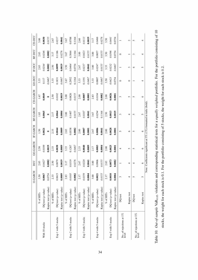
O-G
AR
CH
DC
CG
O-G
AR
CH
IF-G
AR
CH
BF-
GA
RC
HC
D-G
AR
CH
GO
-DC
CIF
-DC
CB
F-D
CC
CD
-DC
C
With
10st
ocks
%of
HIT
s3.
502.
832.
501.
501.
831.
673.
332.
832.
833.
00
DQ
test
(p-v
alue
)0.
0067
0.04
270.
0109
0.00
210.
0065
0.00
490.
117
0.02
440.
0246
0.00
30
Kup
iec
test
(p-v
alue
)0.
0754
0.00
820.
0019
00
00.
0467
0.00
820.
0082
0.01
55
Exp
1w
ith5
stoc
ks
%of
HIT
s2.
332.
502.
332.
332.
172.
503.
332.
503.
172.
67
DQ
test
(p-v
alue
)0.
0615
0.08
790.
0038
0.00
440.
0064
0.01
020.
1831
0.00
990.
1186
0.02
17
Kup
iec
test
(p-v
alue
)0.
0009
0.00
190.
0009
0.00
090.
0004
0.00
190.
0467
0.00
190.
0276
0.00
41
Exp
2w
ith5
stoc
ks
%of
HIT
s2.
833.
173.
332.
833.
003.
003.
673.
503.
673.
67
DQ
test
(p-v
alue
)0.
0105
0.03
190.
1267
0.05
380.
1407
0.08
260.
2952
0.04
640.
3044
0.07
88
Kup
iec
test
(p-v
alue
)0.
0082
0.02
760.
0467
0.00
820.
0155
0.01
550.
1164
0.07
540.
1164
0.11
64
Exp
3w
ith5
stoc
ks
%of
HIT
s2.
172.
672.
332.
002.
672.
003.
332.
673.
002.
60
DQ
test
(p-v
alue
)0.
0359
0.02
200.
0040
0.00
070.
0107
0.00
070.
1191
0.02
370.
0423
0.01
13
Kup
iec
test
(p-v
alue
)0.
0004
0.00
410.
0009
0.00
010.
0041
0.00
010.
0467
0.00
410.
0155
0.00
19
Exp
4w
ith5
stoc
ks
%of
HIT
s3.
003.
002.
172.
673.
672.
833.
333.
003.
003.
17
DQ
test
(p-v
alue
)0.
0021
0.09
060.
0083
0.00
860.
0294
0.01
840.
0807
0.02
470.
0857
0.04
66
Kup
iec
test
(p-v
alue
)0.
0155
0.01
550.
0004
0.00
410.
1164
0.00
820.
0467
0.01
550.
0155
0.02
76
Exp
5w
ith5
stoc
ks
%of
HIT
s2.
172.
832.
002.
002.
502.
003.
503.
333.
503.
50
DQ
test
(p-v
alue
)0.
0010
0.00
730.
0025
0.00
280.
0013
0.00
260.
0423
0.02
320.
0396
0.04
41
Kup
iec
test
(p-v
alue
)0.
0004
0.00
820.
0001
0.00
010.
0019
0.00
010.
0754
0.04
670.
0754
0.07
54
No.
ofre
ject
ions
at1%
leve
l
DQ
test
31
45
33
01
01
Kup
iec
test
44
56
45
03
12
No.
ofre
ject
ions
at5%
leve
l
DQ
test
54
55
55
16
35
Kup
iec
test
56
66
56
45
44
Not
e:C
oeffi
cien
tssi
gnifi
cant
at5%
(1%
)for
mat
ted
inita
lic(b
old)
.
Tabl
e10
:O
ut-o
f-sa
mpl
eV
aR0.0
5vi
olat
ions
and
corr
espo
ndin
gst
atis
tical
test
sfo
ra
equa
llyw
eigh
ted
port
folio
.Fo
rth
epo
rtfo
lioco
nsis
ting
of10
stoc
ks,t
hew
eigh
tfor
each
stoc
kis
0.1.
Fort
hepo
rtfo
lioco
nsis
ting
of5
stoc
ks,t
hew
eigh
tfor
each
stoc
kis
0.2.
34

7. Conclusion
In this paper we consider the estimation problem of GARCH models from the information-
theoretic viewpoint. We reveal the relationship between the statistical dependence in standard-
ized residuals and the maximum likelihood when estimating univariate or multivariate GARCH
models. We show that maximizing the likelihood is equivalent to minimizing the statistical de-
pendence in standardized residuals. In particular, we focus on the framework of the general-
ized orthogonal GARCH and propose three efficient models in this framework. These models
are independent-factor GARCH, best-factor GARCH, and conditional-decorrelation GARCH.
Independent-factor GARCH exploits ICA to make factors mutually as independent as possible.
Best-factor GARCH gives the factors which have the largest autocorrelation in their squared
values such that their volatilities are forecasted well by univariate GARCH. And conditional-
decorrelation GARCH aims at ensuring that factors are not only unconditionally uncorrelated,
but also conditionally as uncorrelated as possible. These models exploit the data information
from different aspects to construct factors, and the factors are all estimated fast and feasibly and
they have clear statistical properties.
We further exploit the DCC model to estimate the weak conditional correlation between fac-
tors and develop factor-DCC models. We explain that such models give better performance than
the original factor GARCH and DCC. Experimental results on the Hong Kong stock market with
various GARCH models give the following findings: (1) among DCC and factor GARCH mod-
els, conditional-decorrelation GARCH, independent-factor GARCH, and DCC exhibit the best
generalization performance; (2) each factor-DCC model has better performance than DCC and
the corresponding factor GARCH model; (3) conditional-decorrelation GARCH (among factor
GARCH models) and its extension embedded with the DCC model (among factor-DCC models)
provide the best results. The independent-factor GARCH and its extension with DCC embedded
are also recommended since their performance is very close to the best and their estimation is
very fast.
APPENDIX
Proof of Thoerem 1: As git, i = 1, ..., k, are independent, the variance of xt is σ2. According
to the property of cumulants (Nikias & Mendel, 1993),x cumulants of the sum of statistically
x. The fourth-order cross-cumulant of the zero-mean series yit is given by
cum(yit, yit, yi,t−τ , yi,t−τ ) = E{y2it, y
2i,t−τ} − E{y2
it}E{y2i,t−τ} − 2(E{yityi,t−τ})2 (34)
35

independent variables equal the sum of the cumulants of the individual variables. Consequently,
for any τ , we have
cov[( xt
std(xt))2
,( xt−τ
std(xt))2
]
=1σ4
cum(xt, xt, xt−τ , xt−τ )
=1σ4
k∑
i=1
cum(git, git, gi,t−τ , gi,t−τ ) (as g1t, ..., gkt are independent)
=1σ4
k∑
i=1
σ4i cov
[( git
std(git))2
,( gi,t−τ
std(git))2
]
≤ maxi
{cov
[( git
std(git))2
,( gi,t−τ
std(git))2
]}·∑k
i=1 σ4i
σ4→ 0, when k →∞.
Therefore (1) is true. Note that for zero-mean variable x, var(x2) = E{x4}−E[x2]2 = E[x2]2 ·κ(x) + 2E[x2]2. We further have
corr(x2t , x
2t−τ ) =
1var(x2
t )cum(xt, xt, xt−τ , xt−τ )
=1
var(x2t )
k∑
i=1
var(g2it)corr(g2
it, g2i,t−τ )
≤ maxi
[corr(g2it, g
2i,t−τ )] ·
∑ki=1 var(g2
it)var(x2
t )
= maxi
[corr(g2it, g
2i,t−τ )] ·
∑ki=1 σ4
i κ(git) + 2∑k
i=1 σ4i
σ4κ(xt) + 2σ4
= maxi
[corr(g2it, g
2i,t−τ )] ·
∑ki=1 σ4
i κ(git) + 2∑k
i=1 σ4i∑k
i=1 σ4i κ(git) + 2σ4
≤ maxi
[corr(g2it, g
2i,t−τ )] ·
maxi κ(git) + 2maxi κ(git) + 2 σ4∑k
i=1 σ4i
→ 0, when k →∞.
This means that the autocorrelation of x2t also tends to zero as k →∞. ¤
References
Alexander, C. (2000). Orthogonal methods for generating large positive semi-definite covariance
matrices. In ISMA center discussioni papers in finance 2000-06. University of Reading, UK.
available from http://www.ismacentre.rdg.ac.uk.
where τ is the time lag. If yit is temporally uncorrelated, this cumulant is equal to the
autocovariance cov(y2it, y
2i,t−τ ). As its special case, the fourth-order cumulant of yit is
κ4(yi) = E{y4i } − 3E[y2
i ]2.
36

Alexander, C. (2001). Market models: A guide to financial data analysis. Chichester, UK: Wiley.
Baba, Y., Engle, R. F., Kraft, D. F., & Kroner, K. F. (1991). Multivariate simultaneous generalized
ARCH. Unpublished manuscript, Dept. of Economics, University of California, San Diego.
Back, A. D. (1997). A first application of independent component analysis to extracting structure
from stock returns. International Journal of Neural Systems, 8, 473–484.
Bauwens, L., Laurent, S., & Rombouts, J. V. K. (2006). Multivariate GARCH models: A survey.
Journal of Applied Econometrics, 21, 79–109.
Bell, A. J., & Sejnowski, T. J. (1995). An information-maximization approach to blind separation
and blind deconvolution. Neural Computation, 7, 1129–1159.
Bera, A., & Higgins, M. (1993). ARCH models: Properties, estimation and testing. Journal of
Economic Surveys, 7, 305–366.
Bollerslev, T. (1986). A generalized autoregressive conditional heteroskedasticity. Journal of
Econometrics, 31, 307–327.
Bollerslev, T. (1990). Modeling the coherence in short-run nominal exchange rates: A multivari-
ate generalized ARCH approach. Review of Economics and Statistics, 72, 498–505.
Bollerslev, T., Chou, R., & Kroner, K. (1992). ARCH modeling in finance: A review of the theory
and empirical evidence. Journal of Econometrics, 52, 5–59.
Bollerslev, T., Engle, R. F., & Nelson, D. B. (1994). ARCH models. In R. F. Engle and D. Mc-
Fadden (Eds.), Handbook of econometrics, vol. 4, 2959–3038. North-Holland, Amsterdam.
Bollerslev, T., Engle, R. F., & Wooldridge, J. (1988). A capital asset pricing model with time-
varying covariances. Journal of Political Economy, 96, 116–131.
Bollerslev, T., & Wooldridge, J. (1992). Quasi-maximum likelihood estimation and inference in
dynamic models with time-varying covariances. Econometric Reviews, 11, 143–179.
Brock, W. A., Dechert, W. D., Sheinkman, J. A., & LeBaron, B. (1996). A test for independence
based on the correlation dimension. Econometric Reviews, 15, 197–235.
Cardoso, J. F., & Souloumiac, A. (1993). Blind beamforming for non-Gaussian signals. IEE
Proceeding-F, 140, 362–370.
37

Cardoso, J. F., & Souloumiac, A. (1996). Jacobi angles for simultaneous diagonalization. SIAM
J. Mat. Anal. Appl., 17, 161–164.
Cha, S. M., & Chan, L. W. (2000). Applying independent component analysis to factor model in
finance. Intelligent Data Engineering and Automated Learning-IDEAL 2000, Springer, 538–
544.
Chan, L., & Cha, S. (2001). Selection of independent factor model in finance. proceedings of 3rd
International Conference on Independent Component Analysis and blind Signal Separation.
San Diego, California, USA.
Christodoulakis, G. A., & Satchell, S. E. (2002). Correlated ARCH (CorrARCH): Modelling
the time-varying conditional correlation between financial asset returns. European Journal of
Operational Research, 139, 351–370.
Cichocki, A., & Amari, S. (2003). Adaptive blind signal and image processing: Learning algo-
rithms and applications. UK: John Wiley & Sons. corrected and revisited edition edition.
Cover, T. M., & Thomas, J. A. (1991). Elements of information theory. Wiley.
Darbellay, G., & Wuertz, D. (2000). The entropy as a tool for analyzing statistical dependencies
in financial time series. Physica A, 287, 429–439.
Ding, Z. (1994). Time series analysis of speculative returns. PhD dissertation, University of
Califoria, San Diego.
Dionısio, A., Menezes, R., & Mendes, D. (2003). Mutual information: A dependence measure
for nonlinear time series. Economics Working Paper Archive at WUSTL, 0311003.
Engle, R. (1982). Autoregressive conditional heteroscedasticity with estimates of the variance of
u.k. inflation. Econometrica, 50, 987–1008.
Engle, R., & Gonzalez-rivera, G. (1991). Semiparametric ARCH models. Journal of Business
and Economic Statistics, 9, 345–359.
Engle, R., & Manganelli, S. (2004). Caviar: Conditional autoregressive value at risk by regression
quantiles. Journal of Business and Economic Statistics, 22, 367–381.
Engle, R. F. (2002). Dynamic conditional correlation: A simple class of multivariate GARCH
models. Journal of Business and Economic Statistics, 20, 339–350.
38

Engle, R. F., & Kroner, K. F. (1995). Multivariate simultaneous generalized ARCH. Econometric
Theory, 11, 122–150.
Engle, R. F., Ng, V. K., & Rothschild, M. (1990). Asset pricing with a factor ARCH covariance
structure: Empirical estimates for treasury bills. Journal of Econometrics, 45, 213C238.
Fan, J., Wang, M., & Yao, Q. (2005). Modelling multivariate volatilities via conditionally uncor-
related components. unpublished manuscript.
Hyvarinen, A. (2001). Blind source separation by nonstationarity of variance: A cumulant based
approach. IEEE Transaction on Neural Networks, 12, 1471–1474.
Hyvarinen, A., Karhunen, J., & Oja, E. (2001). Independent component analysis. John Wiley &
Sons, Inc.
Hyvarinen, A., & Oja, E. (1997). A fast fixed-point algorithm for independent component analy-
sis. Neural Computation, 9, 1483–1492.
Jerez, M., Casals, J., & Sotoca, S. (2000). The likelihood of multivariate GARCH models is
ill-conditioned. Preliminary version.
Kiviluoto, K., & Oja, E. (1998). Independent component analysis for parallel financial time
series. Proc. ICONIP’98 (pp. 895–898). Tokyo, Japan.
Kupiec, P. (1995). Techniques for verifying the accuracy of risk measurement models. The
Journal of Derivatives, 3, 73–84.
Lanne, M., & Saikkonen, P. (2005). A multivariate generalized orthogonal factor GARCH model.
In Discussion paper no 63, helsinki center of economic research. ISSN 1795-0562.
Long, X. D. (2005). Semiparametric multivariate GARCH model. FMA European Conference.
Maasoumi, E., & Racine, J. (2002). Entropy and predictability of stock market returns. Journal
of Econometrics, 107, 291–312.
Matsuoka, K., Ohya, M., & Kawamoto, M. (1995). A neural net for blind separation of nonsta-
tionary signals. Neural Networks, 8, 411–419.
Nelson, D. (1991). Conditional heteroskedasticity in asset returns: A new approach. Economet-
rica, 59, 347ł370.
39

Nelson, D., & Cao, C. (1992). Inequality constraints in the univariate GARCH model. Journal
of Business and Economic Statistics, 10, 229–235.
Nikias, C., & Mendel, J. (1993). Signal processing with higher-order spectra. IEEE Signal
Processing Magazine, 10, 10–37.
Poon, S., & Granger, C. W. (2003). Forecasting volatility in financial markets: A review. Journal
of Economic Literature, 41, 478–539.
Rombouts, J., & Verbeek, M. (2004). Evaluating portfolio value-at-risk using semi-parametric
garch models. available at http://neumann.hec.ca/iea/cahiers/2004/iea0414 jrom.pdf.
Sheppard, K. (2002). Ucsd garch toolbox, version 2.0, 01-Jan-2002. available at
http://www.kevinsheppard.com/research/ucsd garch/ucsd garch.aspx.
Taleb, A., Sole, J., & Jutten, C. (2001). Quasi-nonparametric blind inversion of Wiener systems.
IEEE Transaction on Signal Processing, 49, 917–924.
Tse, Y. K., & Tsui, K. C. (2002). A multivariate GARCH model with time-varying correlations.
Journal of Business and Economic Statistics, 20, 351–362.
van der Weide, R. (2002). GO-GARCH: a multivariate generalized orthogonal GARCH model.
Journal of Applied Econometrics, 17, 549–564.
40