at SciVerse ScienceDirect

Atmospheric Environment 60 (2012) 109e120

Contents lists available

Atmospheric Environment

journal homepage: www.elsevier .com/locate/atmosenv

Effects of light duty gasoline vehicle emission standards in the United States onozone and particulate matter

Krish Vijayaraghavan*, Chris Lindhjem, Allison DenBleyker, Uarporn Nopmongcol, John Grant,Edward Tai, Greg YarwoodENVIRON International Corporation, 773 San Marin Drive, Suite 2115, Novato, CA 94998, USA

h i g h l i g h t s

< Simulations of the incremental benefits of successive US LDV emissions standards.< Tier 1, Tier 2, hypothetical nationwide LEV III standard and zero-out LDV scenario.< Calculated ozone and PM reductions assuming each standard is prevailing in 2022.< Tier 2 to LEV III switch offers very small benefit compared to Tier 1 to 2 change.< Benefit of eliminating LDVs is smaller than the benefit from Tier 1 to 2 transition.

a r t i c l e i n f o

Article history:Received 29 February 2012Received in revised form30 May 2012Accepted 30 May 2012

Keywords:LEVTier 2LDVCAMxMOVESOzonePM2.5

* Corresponding author. Tel.: þ1 415 899 0700.E-mail address: krish@environcorp.com (K. Vijaya

1352-2310/$ e see front matter � 2012 Elsevier Ltd.http://dx.doi.org/10.1016/j.atmosenv.2012.05.049

a b s t r a c t

More stringent motor vehicle emission standards are being considered in the United States to attainnational air quality standards for ozone and PM2.5. We modeled past, present and potential future USemission standards for on-road gasoline-fueled light duty vehicles (including both cars and light trucks)(LDVs) to assess incremental air quality benefits in the eastern US in 2022. The modeling results show thatlarge benefits in ozone and PM2.5 (up to 16 ppb (14%) reductions in daily maximum 8-h ozone, up to10 ppb (11%) reductions in the monthly mean of daily maximum 8-h ozone, up to 4.5 mg m�3 (9%)reductions in maximum 24-h PM2.5 and up to 2.1 mg m�3 (10%) reductions in the monthly mean PM2.5)accrued from the transition from Tier 1 to Tier 2 standards. However, the implementation of additionalnationwide LDV controls similar to draft proposed California LEV III regulations would result in very smalladditional improvements in air quality by 2022 (up to 0.3 ppb (0.3%) reductions in daily maximum 8-hozone, up to 0.2 ppb (0.2%) reductions in the monthly mean of daily maximum 8-h ozone, up to0.1 mg m�3 (0.5%) reductions in maximum 24-h PM2.5 and up to 0.1 mg m�3 (0.5%) reductions in themonthly mean PM2.5). The complete elimination of gasoline-fueled LDV emissions in 2022 is predicted toresult in improvements in air quality (up to 7 ppb (8%) reductions in daily maximum 8-h ozone, up to4 ppb (6%) reductions in the monthly mean of daily maximum 8-h ozone, up to 2.8 mg m�3 (7%) reductionsin maximum 24-h PM2.5 and up to 1.8 mg m�3 (8%) reductions in the monthly mean PM2.5) from Tier 2levels, that are generally smaller than the improvements obtained in switching from Tier 1 to Tier 2.

� 2012 Elsevier Ltd. All rights reserved.

1. Introduction

Emissions from on-road motor vehicles in the United States (US)have decreased significantly over the past four decades even withincreases in traffic volume. For example, highway vehicle emissionsof volatile organic compounds (VOCs) decreased by approximately75% from 1970 to 2005 and emissions of particulate matter (PM)

raghavan).

All rights reserved.

and nitrogen oxides (NOx) decreased by over 50% though totalVehicles Miles Traveled (VMT) for highway vehicles increasedmorethan two-fold (Kryak et al., 2010). These emissions reductions havebeen due, in large part, to increasingly stricter emissions and fuelstandards for gasoline-fueled light duty vehicles (LDVs) in the USsince the 1970s. The aim of these standards is to improve ambientair quality as emissions of VOCs, NOx and PM from LDVs are oftenkey precursors to ambient ozone (O3) and fine particulate matter(PM2.5). With the potential lowering of the National Ambient AirQuality Standards (NAAQS) for 8-h O3 and PM2.5, States would likelyseek additional means to reach or stay in O3 and PM attainmentincluding possibly adopting more severe LDV emission standards.

K. Vijayaraghavan et al. / Atmospheric Environment 60 (2012) 109e120110

Therefore, it is of interest to understand the incremental O3 andPM2.5 benefits of past and current LDV emissions standards and theadditional air quality benefits of potential future LDV emissionsstandards in the US.

While other modeling studies have analyzed the contribution ofmotor vehicles to O3 and/or PM2.5 concentrations and the impact ofvehicle fuel and emissions controls on these concentrations (e.g.,EPA,1999; Matthes et al., 2007; Koffi et al., 2010; Nopmongcol et al.,2011; Roustan et al., 2011; Collet et al., 2012), the current workprovides a cohesive analysis of the effect of historical, current andpotential future LDV emissions standards on O3 and PM2.5 in the US.We apply state-of-the-science emissions models and an advancedregional 3-D photochemical air quality model that simulatestransport and dispersion, atmospheric chemical transformation,and deposition to the earth’s surface of trace gases and aerosols, toestimate impacts of different LDV emissions standards on ozoneand primary and secondary PM in the eastern US with a focus onAtlanta, Detroit, Philadelphia and St. Louis. A 2008 baseline is usedfor air quality model performance evaluation. Four future yearemissions scenarios with increasingly stricter emission standardsfor gasoline-fueled LDVs are compared against each other to esti-mate the incremental and cumulative effect of LDV emissionscontrols on ambient air quality.

2. Methods

2.1. Modeling domain and emissions scenarios

The air quality simulations were conducted with the Compre-hensive Air Quality Model with Extensions (CAMx) (ENVIRON,2011) using on-road emissions inventories derived using theMotor Vehicle Emission Simulator (MOVES) (EPA, 2010a) and othermodel inputs as discussed below. We applied version 5.40 of CAMxwith the Carbon Bond 5 (CB05) chemical mechanism and version2010a of MOVES.

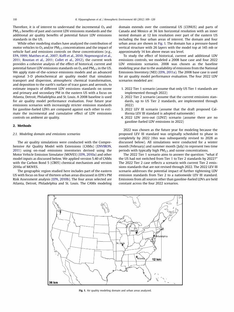
The geographic region studied here includes part of the easternUS with focus on four of thirteen urban areas discussed in EPA’s PMRisk Assessment analysis (EPA, 2010b). The four areas selected areAtlanta, Detroit, Philadelphia and St. Louis. The CAMx modeling

Fig. 1. Air quality modeling doma

domain extends over the continental US (CONUS) and parts ofCanada and Mexico at 36 km horizontal resolution with an innernested domain at 12 km resolution over part of the eastern USincluding the four urban areas of interest. The domain and foururban areas are shown in Fig. 1. The domain has a pressure-basedvertical structure with 26 layers with the model top at 145 mb orapproximately 14 km above mean sea level.

To study the effect of historical, current and additional LDVemissions controls, we modeled a 2008 base case and four 2022LDV emissions scenarios. 2008 was chosen as the baselinemodeling year due to the availability of emissions from the NationalEmissions Inventory (NEI) (EPA, 2011a). The 2008 base case is usedfor air quality model performance evaluation. The four 2022 LDVscenarios modeled are:

1. 2022 Tier 1 scenario (assume that only US Tier 1 standards areimplemented through 2022)

2. 2022 Tier 2 scenario (assume that the current emissions stan-dards, up to US Tier 2 standards, are implemented through2022)

3. 2022 LEV III scenario (assume that the draft proposed Cal-ifornia LEV III standard is adopted nationwide)

4. 2022 LDV zero-out (LDVZ) scenario (assume there are nogasoline-fueled LDV emissions in 2022)

2022 was chosen as the future year for modeling because theproposed LEV III standard was originally scheduled to phase incompletely by 2022 (this was subsequently revised to 2028 asdiscussed below). All simulations were conducted for a wintermonth (February) and summer month (July) to represent two timeperiods with typically high PM2.5 and ozone concentrations.

The 2022 Tier 1 scenario aims to answer the question: “what ifthe US had not switched from Tier 1 to Tier 2 standards by 2022?”The 2022 Tier 2 case reflects a scenario with current Tier 2 emis-sions standards that are not revised through 2022. The 2022 LEV IIIscenario addresses the potential impact of further tightening LDVemission standards from Tier 2 to a nationwide LEV III standard.Emissions from all sources other than gasoline-fueled LDVs are heldconstant across the four 2022 scenarios.

in and urban areas analyzed.

K. Vijayaraghavan et al. / Atmospheric Environment 60 (2012) 109e120 111

The Tier 1 program instituted standards for Total Hydrocarbons,carbon monoxide (CO), NOx and PM for 1994e2003 model yearvehicles with a phase-in for the early years. Tier 2 applied to modelyears 2004 onwards and phased in completely in 2009. The draftproposed California LEV III standards will apply to vehicle modelyears 2015e2028. The exhaust emission standards for the Tier 1and 2 programs for gasoline-fueled LDVs and the draft proposedCalifornia LEV III standards are shown in Table S1.1 (where “S”refers to Supplementary data).

2.2. Meteorology

CAMx modeling for 2008 and the 2022 scenarios was drivenby year 2008 meteorological fields from the Weather Researchand Forecast (WRF) model e Advanced Research WRF (ARW)core (Skamarock et al., 2008). WRF output meteorological fieldsat 12 km horizontal resolution over the CONUS were obtainedfrom the EPA (Gilliam, R., personal communication, 2011) andconverted to CAMx input meteorological files for the nested 36and 12 km resolution domains. The WRF and CAMx vertical gridstructure and mapping from WRF to CAMx layers are shown inTable S4.1. A limited performance evaluation of the WRF mete-orological outputs and CAMx-ready meteorology showed satis-factory performance (see S4. in Supplementary data foradditional information).

2.3. On-road motor vehicle emissions

MOVES 2010a was used to prepare on-road emissions invento-ries in the CONUS for the 2008 base case and the four 2022 emis-sions scenarios. MOVES was run for calendar years 2008 and 2022for vehicle ages 0e30 to develop on-road vehicle emissions for the2008 base case and 2022 Tier 2 scenario. Tier 1 emission factors forvehicle model years after 2000 do not exist by default in MOVESandwere simulated as existing in 2022 by runningmultiple historiccalendar years in MOVES keeping all other model assumptions thesame as they are in 2022. Ratios of LEV III to LEV II emissionscalculated using simulations with the California Air ResourcesBoard’s Emissions Factor Model (EMFAC2007) (http://arb.ca.gov/msei/onroad/latest_version.htm, accessed August 2011) wereused to adjust MOVESmodel LEV II emission rate input estimates tocalculate emission rates for the 2022 LEV III scenario. On-roademissions in the zero-out LDV scenario were computed by settingemissions of Source Classification Codes (SCCs) corresponding togasoline-fueled LDVs to zero in the 2022 Tier 2 emissions. Detailedinformation on the calculation of on-road emissions in the variousscenarios is provided in the Supplementary data.

The on-road emissions for winter and summer from MOVES forall emissions scenarios were speciated to CAMx model species,temporally allocated to hourly emissions and spatially allocated togrid cells using version 2.7 of the Sparse Matrix Operator KernelEmissions (SMOKE) model. Average day emissions were adjusted toaccount for day-of-week and hour-of-day effects based on SCCcodes. Emission estimates for total VOCwere converted to the CB05chemical mechanism in CAMx using VOC speciation profilesderived from EPA’s SPECIATE database, version 4.3 (EPA, 2011b)(see Table S5.1). PM emissions were speciated to CAMx modelspecies, namely primary organic aerosol, primary elementalcarbon, primary nitrate, primary sulfate, primary fine other PM andcoarse PM following methods outlined by Baek and DenBleyker(2010). On-road mobile sources generated using MOVES at thecounty level were allocated to CAMx 36 km and 12 km grid cellsusing spatial surrogates derived with the Spatial Surrogate Tool(http://www.epa.gov/ttn/chief/emch/spatial/spatialsurrogate.html,accessed August 2011).

Canadian on-road emissions for the 2008 and 2022 scenarioswithin the 36 km grid were derived from the 2005 NEI and 2020NEI, respectively (see below). Mexican on-road emissions withinthe 36 km grid for all scenarios were derived from the 2005 NEI andbased on 2000 emissions.

2.4. Other emissions

Emissions from anthropogenic area and point sources in 2008 inthe CONUS were developed from version 1.5 of the 2008 NEI (EPA,2011a). Emissions from these source categories for the 2022emissions scenarios were prepared from the 2020 NEI inventory(EPA, 2010c) and held constant from 2020 to 2022. The 2020 NEIwas developed by EPA by projecting the 2005-based v4 modelingplatform emissions to 2020. Anthropogenic area and point emis-sions for Canada for the 2008 base case and 2022 scenarios withinthe 36 km grid were prepared from and set equal to emissions inthe 2005 NEI (EPA, 2011c) and the 2020 NEI, respectively. Anthro-pogenic area and point emissions for Mexico within the 36 km gridfor the 2008 base case were prepared from the 2005 NEI and heldconstant between the 2008 and 2022 scenarios due to lack ofadditional information. Emissions outside the 36 km grid aretreated through the boundary conditions (see below).

We developed 2008 non-road mobile source emissions in theCONUS from the 2008 NEI. The NEI non-road emissions are basedon the National Mobile Inventory Model (NMIM) using countyspecific fuel properties, meteorological parameters and non-defaultlocal activity data for areas where such activity data has beenprovided to EPA as part of its NEI development efforts. We used theNMIM model to generate county level estimates of 2022 non-roademissions in the CONUS for February and July. 2008 emissions fromlocomotives/harbor craft, aircraft and commercial marine vesselswere also obtained from the 2008 NEI. 2022 emissions from loco-motives/harbor craft, aircraft and commercial marine vessels wereobtained from the 2020 NEI and forecast two years through 2022following forecast methods applied by EPA (2008a), FAA (2010) andEPA (2009), respectively.

Biogenic emissions in 2008 across the CONUS and the parts ofCanada and Mexico in the CAMx 36 km domain were developedusing the Model of Emissions of Gases and Aerosols from Nature(MEGAN v. 2.04; Guenther et al., 2006). MEGAN uses griddedemission factors that are based on global datasets for 11 species(CO, nitric oxide, isoprene and other VOCs) and 4 functional planttypes and plant leaf area index. Biogenic emissions were heldconstant from 2008 to 2022. Wildfire emission inventories of CO,NOx, VOCs, SO2, NH3 and PM in North America for 2008 werederived from the Blue Sky Framework SMARTFIRE database (http://www.getbluesky.org/smartfire) and processed using version 3.12 ofthe Emissions Processing System (EPS) tool (ENVIRON, 2009).Wildfire emissions were held constant in all emissions scenarios.Sea salt emissions inventories of particulate sodium, chloride andsulfate for 2008 were prepared using the meteorological fieldsdriven by WRF (temperature, pressure, winds) and land coverinformation. Sea salt emissions were also not altered from the 2008to 2022 scenarios.

The emissions inventories described above were converted tospeciated, gridded, temporally varying emissions files suitable forair quality modeling with CAMx in the nested 36/12 km domainsfollowing standard emissions processing methods described in theliterature (e.g., Morris et al., 2007; 2008).

2.5. Other model inputs

Boundary concentrations of O3, PM components and precursorsfor February and July 2008 (in addition to a 15-day model spin-up

K. Vijayaraghavan et al. / Atmospheric Environment 60 (2012) 109e120112

in each case) for the CAMx 36 km domain were derived from theglobal chemical and transport model, Model for Ozone and RelatedChemical Tracers (MOZART) version 4.6 (Emmons et al., 2010).Six-hourly model outputs in a latitude-longitude coordinatesystemwith a spatial resolution of about 2.8� for both latitude andlongitude and 28 vertical layers were mapped onto the CAMxdomain and speciated for the CB05 chemical mechanism. Theboundary conditions for the 36 km domain were kept constantacross all scenarios. Boundary conditions for the 12 km domain arecalculated within CAMx from the 36 km grid calculations in eachscenario.

The landuse/landcover (LULC) databases used in biogenicemissions inventory preparation and CAMx modeling wereobtained from the National Land Cover Dataset (NLCD) (http://www.mrlc.gov/nlcd06_data.php, accessed July 2011). The datawere processed andmapped to the 26 landuse categories in the drydeposition scheme of Zhang et al. (2003) used in CAMx. Photolysisrates required for ozone modeling were developed using the CAMxphotolysis rate pre-processor, which incorporates the TroposphericUltraviolet and Visible (TUV) radiative transfer model (NCAR, 2011).

3. Results and discussion

3.1. Emissions and air quality in 2008

3.1.1. EmissionsFig. 2 presents the total anthropogenic emissions estimated in

the CONUS and the fractions of the major source categories inFebruary and July 2008. The sectors shown include area sources(comprising residential, commercial and small industrial sources),electric generating units (EGU), stationary point sources other thanEGUs (abbreviated here as non-EGU Pt), off-road sources, LDVs andother on-road sources. The modeled emission totals across theCONUS are generally consistent with totals provided by EPA for theNEI (http://neibrowser.epa.gov, accessed September 2011); differ-ences are mainly in the on-road sector. EPA developed the NEI on-road sector emissions data using the NMIM, which uses theMOBILE6 vehicle emissions model whereas this study uses themore current MOVESmodel. The on-road fraction (LDV plus others)of the total 2008 US anthropogenic inventory varies considerablyacross pollutants; it is high for CO (52e60%) and NOx (40e41%) andvery low for SO2 (<0.5%). Pollutants exhibit seasonal effects. TotalCO emissions decrease by 14% from winter to summer; this isprimarily due to a 25% seasonal decrease in on-road emissionsassociated partly with fewer cold starts in summer. Total NH3emissions increase more than two-fold from winter to summer.This is due, in part, to higher dairy NH3 emissions in summer thanwinter (Pinder et al., 2004). Primary PM2.5 emissions from LDVsdecrease from winter to summer due to the increase in ambienttemperatures as discussed below.

The modeled spatial distribution of on-road emissions in theeastern US in the 2008 base case shows the urban signature of on-road emissions, in particular in Atlanta, Chicago, Detroit, Indian-apolis, St. Louis and along the eastern seaboard (see Fig. S7.1). NOxemissions are higher in summer than winter (by 5e10% or more)because higher running exhaust NOx in summer more thancompensate for higher cold start emissions in winter. However, on-road emissions of VOCs and PM2.5 decrease fromwinter to summerby up to 20%e30% in some urban areas such as in the New York/New Jersey. These seasonal trends are also evident in the 2008emissions inventory for gasoline-fueled LDVs both across theCONUS (Table 1) and in the four urban areas of interest (Table 2).

Table 1 also shows the LDV fraction of total on-road and totalanthropogenic emissions. Gasoline-fueled LDV emissions of NOxand VOC constitutew20% of total anthropogenic emissions in 2008

and, hence, are important to studying the potential contribution ofLDVs to ambient O3 and PM2.5. Due to their slow reactivity, COemissions have a much more limited effect on O3 concentrations.While primary PM2.5 emissions from LDVs can directly affectambient PM2.5, these represent a very small fraction (2%) of thetotal anthropogenic inventory; there is a much larger PM contri-bution from stationary sources, wood-burning, non-road sources,road dust and other sources. LDV emissions of NH3 and SO2constitute a large fraction (70e90%) of total on-road emissions.However, they represent a very small fraction (0.3e5%) of totalanthropogenic emissions due to the dominance of other sourcessuch as livestock farming and fuel combustion.

St. Louis has the highest NOx, VOC and PM2.5 emissions amongthe four urban areas as shown in Table 2 (values shown representthe total across the counties in each metropolitan area). However,MOVES default age distributions were used for St. Louis while localdata on vehicle age distributions were used for other three urbanareas; this likely introduced uncertainty in our estimates for St.Louis. For example, we determined that using local age distribu-tions for Atlanta, Detroit and Philadelphia resulted in modeled VOCemissions that were approximately 10% lower than if we had usedMOVES default age distributions (see Fig. S2.3). Atlanta has thehighest NOx and VOC LDV emissions among the three urban areaswhere local vehicle age distributions were used in MOVESmodeling. In all four urban areas, PM2.5 emissions are higher inwinter than summer by 75% or more. Vehicle testing in KansasCity has shown that PM emissions increase exponentially astemperature decreases with the effect more pronounced for coldstarts (EPA, 2008b).

3.1.2. Air quality in 2008Fig. 3 shows the predicted monthly mean of daily maximum 8-h

average O3 concentrations in winter and summer 2008 in theCONUS at 36 km model resolution and in the eastern US at 12 kmresolution. As expected, O3 levels are low (<50 ppb) in February dueto limited solar radiation and photochemical activity except inColorado and other parts of thewestern USwhere O3 formationmaybe enhanced by shallow inversion with limited mixing and snowcover with high albedo. In July, the predicted monthly mean of dailymaximum 8-h O3 goes up to 95 ppb in the CONUS (with the highestvalue in the Los Angeles basin) and up to 91 ppb over the eastern US(near Washington, D.C.). The predicted monthly averages of dailymaximum8-h O3 in July 2008 are 83 ppb, 59 ppb, 82 ppb and 73 ppbin Atlanta, Detroit, Philadelphia and St. Louis, respectively.

Fig. 4 shows the predicted monthly mean concentrations ofPM2.5 mass in February and July 2008 in the CONUS and eastern US.Figs. S8.1 and S8.2 show similar plots for PM2.5 components inFebruary and July, respectively. The exceptionally high PM2.5concentrations predicted in northern California (>100 mg m�3) inJuly 2008 are due to emissions from extreme wildfire events in thisregion. PM2.5 sulfate concentrations are higher in the eastern US insummer than in winter due to enhanced formation from SO2emissions. With the exception of southern Georgia, organic carbonis generally higher in summer in the Southeast due, in part, tohigher biogenic emissions. PM2.5 nitrate is higher in winter in theupper Midwest caused, in part, by a stronger partitioning of totalnitrate towards the aerosol phase at lower temperatures. WinterPM2.5 concentrations exceed 30 mg m�3 in Georgia, the Chicagometropolitan area and parts of the Northeast. The four urban areasof interest in this study all show comparable monthly averagedPM2.5 concentrations ofw25e27 mg m�3 in February 2008. Primaryorganic aerosol (POA) makes up the largest portion of predictedPM2.5 mass in Atlanta in both winter and summer while nitrate isthe major PM2.5 component in Detroit, Philadelphia and St. Louis inboth seasons.

Fig. 2. Estimated anthropogenic emissions in the continental US in February and July, 2008.

K. Vijayaraghavan et al. / Atmospheric Environment 60 (2012) 109e120 113

Table 1Average-day emissions from gasoline-fueled LDVs in the continental US in model scenarios.

Winter Summer

NOx VOC PM2.5 CO NH3 SO2 NOx VOC PM2.5 CO NH3 SO2

2008LDV emissions (Mg day�1) 8380 7039 242 92,610 272 79 9661 6384 123 68,064 337 99% of all on-road 50% 86% 39% 90% 92% 72% 52% 83% 21% 89% 92% 71%% of total anthropogenic 20% 21% 2% 54% 5% 0.3% 21% 18% 2% 46% 2% 0.4%2022 Tier 1LDV emissions (Mg day�1) 10,422 6127 250 101,288 457 48 12,047 5319 131 73,217 566 57% of all on-road 77% 92% 73% 92% 94% 83% 80% 88% 55% 92% 94% 81%% of total anthropogenic 31.0% 18.6% 2.9% 60% 8% 0.3% 32% 16% 2% 49% 4% 0.3%2022 Tier 2LDV emissions (Mg day�1) 2609 2269 188 69,576 166 41 2897 2247 108 40,745 206 48% of all on-road 46% 81% 67% 89% 86% 80% 49% 75% 51% 87% 86% 79%% of total anthropogenic 10.1% 7.8% 2.2% 51% 3% 0.2% 10% 8% 2% 35% 1% 0.2%2022 LEV IIILDV emissions (Mg day�1) 2505 2134 173 65,152 166 41 2781 2098 103 38,120 206 48% of all on-road 45% 80% 66% 89% 86% 80% 47% 74% 49% 86% 86% 79%% of total anthropogenic 9.7% 7.4% 2.0% 49% 3% 0.2% 10% 7% 1% 33% 1% 0.2%

K. Vijayaraghavan et al. / Atmospheric Environment 60 (2012) 109e120114

The 2008 CAMx base case predictions of 1-h and 8-h averageozone concentrations were evaluated against measurements in theAIRS/AQS network (EPA, 2002) and the Clean Air Status and TrendsNetwork (CASTNET, 2011). Model predictions of PM2.5 mass andcomponents were compared to daily (24-h) average measure-ments in the AIRS/AQS and IMPROVE (IMPROVE, 1995) networks.Overall, model performance was good both for ozone and PM2.5mass and components. Details are provided in the Supplementarydata.

3.2. Emissions and air quality in 2022 scenarios

3.2.1. EmissionsThe total CONUS anthropogenic emissions and the relative

contributions of the major source sectors in the 2022 Tier 2scenario are shown in Fig. 5. Emissions from source sectors otherthan on-road sources are held constant between this scenario andall other 2022 scenarios. Between 2008 and 2022, total anthro-pogenic CONUS emissions are projected to decrease by 37% forNOx, 14% for VOC and 20% for CO (see Figs. 2 and 5). Differencesbetween the 2020/2022 and 2008 inventories are due to bothgrowth and control as well as differences in methodologiesbetween the 2005 inventory (used by EPA to project to 2020) andthe 2008 inventory. The reductions from 2008 to 2022 are ach-ieved, in large part, due to large reductions in the on-road inven-tory reflecting a mature Tier 2 LDV program by 2022. Whenconsidering the average across February and July, the on-road

Table 2Average-day emissions from gasoline-fueled LDVs in four urban areas in 2008.

Urban area Pollutant February 2008 July 2008

Emissions(Mg day�1)

% of allon-road

Emissions(Mg day�1)

% of allon-road

Atlanta NOx 141.8 48% 157.1 51%VOC 103.2 85% 99.8 83%PM2.5 3.9 34% 2.2 20%

Detroit NOx 106.2 41% 107.2 41%VOC 102.6 84% 67.3 77%PM2.5 5.0 40% 1.8 17%

Philadelphia NOx 66.4 55% 73.0 57%VOC 53.1 81% 42.6 74%PM2.5 2.5 48% 1.1 27%

St. Louis NOx 155.8 50% 171.4 52%VOC 120.3 83% 99.8 77%PM2.5 5.4 42% 2.4 22%

fraction of the CONUS NOx anthropogenic inventory decreasesfrom 41% in 2008 to 21% in 2022, while the corresponding fractionsof many of the other source categories are constant or increase. Forexample, the off-road fraction of the CONUS anthropogenic NOxinventory stays constant at w25% from 2008 to 2022. On-roademissions of other pollutants also show a more than propor-tional reduction from 2008 to 2022 (when compared with thereduction in the total inventory) without considering any controlsbeyond Tier 2 (e.g., on-road VOC emissions decrease by 63%, PM2.5by 59% and CO by 31%).

Table 1 shows estimates of emissions from gasoline-fueled LDVsin the CONUS in the 2022 Tier 1, Tier 2 and LEV III scenarios. The2022 Tier 1 scenario represents a hypothetical scenario whereno LDV controls beyond Tier 1 are implemented through 2022.Changes in LDV emissions between the 2008 scenario and the 2022Tier 1 scenario are due to several factors including an approxi-mately 20% increase in nationwide VMT from 2008 to 2022,changes in fleet composition and lower gasoline sulfur in 2022compared to 2008 (MOVES default nationwide average gasolinelevels in 2008 and 2022 are 42 and 21 ppm, respectively). LDVemissions decrease considerably from Tier 1 to Tier 2 and thendecrease only slightly from the Tier 2 to LEV III scenarios. Forexample, on average across winter and summer, LDV NOx emis-sions are reduced by 75% from Tier 1 to Tier 2 and by only 4% fromTier 2 to LEV III. The LDV fraction of the total anthropogenicinventory also decreases considerably from Tier 1 to Tier 2 (e.g., by32% to 10% for NOx and 17% to 8% for VOC on average across winterand summer) and subsequently only marginally from Tier 2 to LEVIII (with the NOx fraction decreasing to 9.9% and VOC to 7.2%).The corresponding predicted spatial distributions of winter andsummer weekday on-road emissions of NOx, VOC and PM2.5 in theCAMx 12 km domain in the 2022 scenarios are presented in theSupplementary data.

Table 3 shows the gasoline-fueled LDV emissions inventory inthe four urban areas in the 2022 LDV emissions scenarios. Winter-time LDV NOx emissions are highest in Atlanta in all scenarios.Wintertime VOC and primary PM2.5 emissions are highest in Detroitdue, in large part, to the effect of colder weather on cold starts. Incontrast, in summer, Atlanta has the highest LDV emissions of NOx,VOC and PM2.5, due to a combination of higher ambient tempera-tures and higher VMT. LDV NOx emissions in all four areas decreasebymore than 70% from Tier 1 toTier 2 and then only by 4% from Tier2 to LEV III. Similarly, VOC emissions decrease by w60% or morefrom Tier 1 to Tier 2 and then by 6e9% in the transition to LEV IIIby 2022.

Fig. 3. Monthly mean of daily maximum 8-h ozone concentrations in the 36 km domain (left) and 12 km domain (right) in February (top) and July (bottom), 2008.

K. Vijayaraghavan et al. / Atmospheric Environment 60 (2012) 109e120 115

3.2.2. Air qualityModel simulation results for O3 are presented in Fig. 6 for the

summer month (July), the time period of concern for O3 in theeastern US. The incremental benefits of the LDV standards areexamined using the spatial distribution of the monthly mean ofdaily maximum 8-h O3 concentrations and differences in thesemonthly means between pairs of 2022 LDV scenarios. The samequantities are listed in Table S9.1 (in Supplementary data) forthe four urban areas. Also shown in this table are the monthlymaximum 8-h O3 concentrations in each area. All values tabulatedfor an urban area are those modeled in the CAMx 12 km resolutiongrid cell in the geographic center of each area reflecting theapproximate impact on the local population.

If LDV emissions standards were nomore stringent than the Tier1 standard in 2022, the monthly mean of daily maximum 8-h O3could be as high as 88 ppb in the portion of the eastern US withinthe CAMx 12 km domain with values exceeding 60 ppb in most ofthe eastern US and parts of Georgia and the New York/New Jersey/D.C. corridor experiencingmore than 80 ppb. Among the four urbanareas analyzed here, the monthly mean of daily maximum 8-h O3ranges from 57 ppb at Detroit to 78 ppb at Philadelphia and thehighest 8-h O3 predicted in the month ranges from 83 ppb inDetroit to 111 ppb in Atlanta.

Strengthening the standard from Tier 1 to Tier 2 results ina reduction of over 6 ppb in the monthly mean of daily 8-h maximain large parts of the eastern US and up to 10 ppb in Georgia (seeFig. 6). When considering only the four areas, Tier 2 ozone benefitsare strongest in Atlanta with the monthly mean of the daily 8-h O3maxima decreasing by 9 ppb (11%) from Tier 1 to Tier 2 and themonthly highest O3 decreasing by 16 ppb (14%) from Tier 1 toTier 2.

When compared to Atlanta and Philadelphia, Detroit shows a smallbenefit (3e4 ppb) for the monthly mean of daily maximum 8-h O3and the monthly highest 8-h O3. St. Louis shows a reduction of5 ppb in the monthly mean but a smaller reduction (2 ppb) in themonthly highest 8-h O3 despite large reductions in NOx (74%) andVOCs (58%) from the Tier 1 to Tier 2 scenarios, suggesting that thehighest 8-h concentration here in the 2022 Tier 1 scenario (94 ppb)is mostly due to sources other than on-road vehicles. There aresome areas on the western shore of Lake Michigan (Milwaukee andChicago) that experience a slight increase (3 ppb) in the monthlymean of daily maximum 8-h O3 from the Tier 1 to Tier 2 scenarios.The increases in ozone in these urban areas despite reductions inLDV NOx emissions from the Tier 1 scenario suggest that NOx thatwas otherwise titrating ozone becomes unavailable due to the Tier2 LDV emissions reductions.

The monthly mean of daily maximum 8-h O3 in the summermonth shows up to a 0.2 ppb (w0.2%) reduction in the eastern USdomain in 2022 if we switch from the Tier 2 to LEV III programs(see Fig. 6). When considering the four urban areas, the predictedreduction in the monthly mean value is w0.1 ppb and themonthly highest 8-h O3 is reduced by 0.1e0.3 ppb (0.1e0.3%) (seeTable S9.1). The model results suggest that there is a very smalladditional benefit in 2022 in strengthening the LDV standard fromTier 2 to one similar to the draft proposed California LEV IIIstandard. These small benefits are consistent with the smallreductions in ozone (<1.5%) modeled by Collet et al. (2012) forthe transition from LEV II to a standard similar to LEV III in theCalifornia South Coast Basin. We note that the LEV III standard forNOx þ non-methane organic gases will not be fully phased inuntil 2025. Thus, results shown represent the air quality benefits

Fig. 4. Monthly mean concentrations of PM2.5 in the 36 km domain (left) and 12 km domain (right) in February (top) and July (bottom), 2008.

K. Vijayaraghavan et al. / Atmospheric Environment 60 (2012) 109e120116

achievable by 2022. We expect some additional improvements inozone from 2022 to 2025 with the planned complete phase-in ofthe LEV III standard.

Eliminating LDV emissions (in the zero-out LDV scenario) resultsin 2e4 ppb (3e5%) reductions in themonthlymean of summertimedaily 8-h maximum ozone and 3e7 ppb (3e8%) in the highest 8-hozone below 2022 Tier 2 levels in the four urban areas. Themaximum reduction in the monthly mean of daily 8-h maximumozone in the eastern US domain is 4 ppb (w6%). The predictedreductions in ozone achieved with the complete zero-out of LDVemissions from the 2022 levels with the current (i.e., Tier 2) stan-dard are generally less than the reductions achieved in movingfrom the Tier 1 to Tier 2 standards.

Model simulation results for PM2.5 mass are shown in Fig. 7 forFebruary and in Fig. 8 for July. We present the spatial distributionof the monthly mean PM2.5 concentrations and differences inthese monthly means between 2022 LDV scenarios. Table S9.1shows similar information for monthly mean PM2.5 and monthlymaximum 24-h PM2.5 in the four urban areas. Table S9.2 showsthe monthly mean concentrations of key PM2.5 components in thefour areas and differences between the scenarios.

Wintertime monthly mean concentrations of PM2.5 in the 2022Tier 1 scenario exceed 15 mg m�3 (the annual mean standard forPM2.5) in large parts of Georgia, the Carolinas, the Northeast and theUpper Midwest (see Fig. 7). Similar spatial patterns are seen in the2022 Tier 2 scenario but the elevated concentrations are lesswidespread. Monthly mean PM2.5 decreases bymore than 1 mg m�3

from Tier 1 to Tier 2 levels in broad swaths across the eastern USand by 2 mg m�3 (w10%) in large urban areas such as Chicago,

Washington D.C., Detroit, Philadelphia and New York. Among thefour urban areas analyzed here, the Tier 1 wintertime mean PM2.5concentration ranges from 14 mg m�3 in Atlanta to 19 mg m�3 inPhiladelphia, and the maximum 24-h PM2.5 ranges from 22 mg m�3

in Atlanta to 48 mg m�3 in Philadelphia (see Table S9.1). WintertimeTier 2 PM2.5 benefits are strongest in Philadelphia with the meanPM2.5 reduced by 1.9 mg m�3 (10%) from Tier 1 levels and maximum24-h PM2.5 reduced by 4.5 mg m�3 (9%). The reductions in PM2.5 dueto Tier 2 are driven by reductions in nitrate in all four urban areas(see Table S9.2). Because nitrate constitutes a very small fraction ofprimary PM emissions, the reduction in nitrate has to be due to thelarge reduction in LDV NOx emissions (see Table 3), which impactssecondary nitrate formation. This is also consistent with relativelyhigh reductions predicted in PM ammonium (compared to theother PM components) which would have otherwise been associ-ated with PM nitrate.

Reductions in PM2.5 concentrations between Tier 1 and Tier 2scenarios are generally lower in summer (Fig. 8) than winter withthe mean PM2.5 in Philadelphia reduced by 0.9 mg m�3 (6%) fromTier 1 levels and maximum 24-h PM2.5 reduced by 1.5 mg m�3 (6%).The Tier 2 PM2.5 benefits in summer are lower primarily due to lessformation of PM nitrate from NOx emissions in summer due toenhanced volatilization from the particulate phase. Also, largerreductions in PM sulfate are predicted in summer (0.1e0.2 mg m�3

reduction in monthly mean) than winter (Table S9.2).Switching from the Tier 2 to LEV III results in less than

0.1 mg m�3 reduction in monthly mean PM2.5 in the eastern USdomain in 2022 in both summer and winter and up to 0.14 mg m�3

(0.5%) reduction inmonthlymaximum 24-h PM2.5 in the four urban

Fig. 5. Estimated anthropogenic emissions in the continental US in the 2022 Tier 2 scenario.

K. Vijayaraghavan et al. / Atmospheric Environment 60 (2012) 109e120 117

Table 3Emissions from gasoline-fueled LDVs in four urban areas in 2022 LDV emissions scenarios.a

Month Area Pollutant LDV Tier 1 emissions(Mg day�1)

LDV Tier 2 emissions(Mg day�1)

LDV LEV III emissions(Mg day�1)

%Change fromTier 1 to Tier 2

%Change fromTier 2 to LEV III

February Atlanta NOx 161 39 37 �76% �4%VOC 92 31 29 �66% �6%PM2.5 3.7 0.8 2.6 �24% �8%

Detroit NOx 152 33 32 �78% �4%VOC 103 33 31 �68% �6%PM2.5 5.2 3.8 3.1 �27% �18%

Philadelphia NOx 83 17 16 �80% �4%VOC 51 18 17 �65% �7%PM2.5 2.6 1.9 1.8 �26% �7%

St. Louis NOx 105 28 27 �73% �4%VOC 67 25 23 �63% �6%PM2.5 3.0 2.2 2.0 �25% �8%

July Atlanta NOx 182 42 41 �77% �4%VOC 81 30 29 �63% �6%PM2.5 2.2 1.9 1.8 �17% �5%

Detroit NOx 156 31 30 �80% �4%VOC 66 26 23 �61% �9%PM2.5 1.9 1.6 1.5 �15% �10%

Philadelphia NOx 91 17 16 �82% �4%VOC 38 15 14 �60% �7%PM2.5 1.2 1.0 1.0 �17% �4%

St. Louis NOx 117 30 29 �74% �4%VOC 53 22 21 �58% �7%PM2.5 1.3 1.1 1.1 �17% �5%

a LDV emissions are all zero in LDV zero-out scenario.

K. Vijayaraghavan et al. / Atmospheric Environment 60 (2012) 109e120118

areas (see Table S9.1). These small changes suggest that littleadditional PM2.5 benefit is obtained by strengthening the LDVstandard from Tier 2 to a LEV III standard. This is consistent withthe relatively small change in PM2.5 precursor emissions betweenthe Tier 2 and LEV III scenarios and the fact that Tier 2 LDVemissions of PM2.5 precursors constitute a relatively small fraction(0.2e10%) of the total inventory (see Table 1). Because the PMcomponent of the draft LEV III standard will not be fully phased inuntil 2028, some additional improvements in PM are expectedfrom 2022 to 2028.

Fig. 6. Monthly mean and differences in monthly mean of daily maximum 8-h ozone concenTier 2 e Tier 1 (bottom left), LEV III e Tier 2 (bottom center), and LDV zero-out e Tier 2 (b

Modeling results suggest that elimination of gasoline-fueled LDVs in the four urban areas would result in0.3e1.5 mg m�3 (3e11%) reductions in the monthly mean PM2.5 and0.3e2.9 mgm�3 (2e7%) in themonthly maximum 24-h PM2.5 below2022 Tier 2 levels. The maximum reduction in the monthly meanPM2.5 in the eastern US domain is 1.8 mg m�3 (w8%). The predictedreductions in total PM2.5 mass due to the complete removal ofgasoline-fueled LDV emissions from 2022 Tier 2 levels are generallyless than the reductions achieved in progressing from the Tier 1 toTier 2 standards.

trations in July in 2022 scenarios: Tier 1 (top left), Tier 2 (top center), LEV III (top right),ottom right).

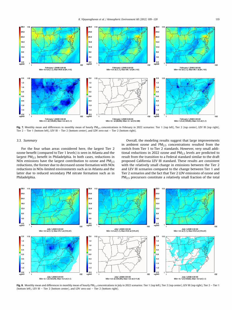
Fig. 7. Monthly mean and differences in monthly mean of hourly PM2.5 concentrations in February in 2022 scenarios: Tier 1 (top left), Tier 2 (top center), LEV III (top right),Tier 2 e Tier 1 (bottom left), LEV III e Tier 2 (bottom center), and LDV zero-out e Tier 2 (bottom right).

K. Vijayaraghavan et al. / Atmospheric Environment 60 (2012) 109e120 119

3.3. Summary

For the four urban areas considered here, the largest Tier 2ozone benefit (compared to Tier 1 levels) is seen in Atlanta and thelargest PM2.5 benefit in Philadelphia. In both cases, reductions inNOx emissions have the largest contribution to ozone and PM2.5reductions, the former due to decreased ozone formationwith NOxreductions in NOx-limited environments such as in Atlanta and thelatter due to reduced secondary PM nitrate formation such as inPhiladelphia.

Fig. 8. Monthly mean and differences in monthly mean of hourly PM2.5 concentrations in July(bottom left), LEV III e Tier 2 (bottom center), and LDV zero-out e Tier 2 (bottom right).

Overall, the modeling results suggest that large improvementsin ambient ozone and PM2.5 concentrations resulted from theswitch from Tier 1 to Tier 2 standards. However, very small addi-tional reductions in 2022 ozone and PM2.5 levels are predicted toresult from the transition to a Federal standard similar to the draftproposed California LEV III standard. These results are consistentwith the relatively small change in emissions between the Tier 2and LEV III scenarios compared to the change between Tier 1 andTier 2 scenarios and the fact that Tier 2 LDV emissions of ozone andPM2.5 precursors constitute a relatively small fraction of the total

in 2022 scenarios: Tier 1 (top left), Tier 2 (top center), LEV III (top right), Tier 2 e Tier 1

K. Vijayaraghavan et al. / Atmospheric Environment 60 (2012) 109e120120

inventory. Predicted improvements in ozone and PM2.5 due to thecomplete elimination of gasoline-fueled LDV emissions are gener-ally smaller than the improvements due to the transition from Tier1 to Tier 2 standards.

The main limitation of this study is introduced by the incom-plete phase-in of the LEV III standard by 2022, the basis year forcomparing emission standards. Some additional improvements inozone from 2023 to 2025 and in PM from 2023 to 2028 areexpected as the LEV III standard fully matures. Other sources ofuncertainty include use of the 2020 NEI as a surrogate for 2022anthropogenic area and point emissions, differences between the2005 base year (which was used to derive the 2020 inventory) andthe 2008 base year and assumed growth and control factors. Thereare also limitations in the data used to develop VOC speciationprofiles. The benefits of the vehicle emissions standards have beendetermined using 2008 meteorology and global backgroundconcentrations. Other meteorological and background conditionsmight yield somewhat different results. We have focused onspecific past, present and potential future Federal standards appliedto the eastern US. Future work should examine whether similarresults are obtained for urban areas in other parts of the countryand consider additional vehicle standards. It would also be useful tocompare the relative contributions of other sources to ozone andPM compared to LDVs.

Acknowledgments

This work was supported by the Coordinating Research CouncilAtmospheric Impacts Committee. We thank Robert Gilliam, EPA fordata on 2008 WRF meteorology and Alison Eyth, EPA for NEI data.

Appendix A. Supplementary data

Additional emissions data, model results and model perfor-mance evaluation can be found in the online version, at http://dx.doi.org/10.1016/j.atmosenv.2012.05.049.

References

Baek, B.H., DenBleyker, A., 2010. User’s Guide for the SMOKE-MOVES IntegrationTool. Prepared for the U.S. EPA OAQPS. July. http://www.smoke-model.org/smoke_moves_tool/SMOKE-MOVES_Tool_Users_Guide.pdf (accessed April2011).

CASTNET, 2011. Clean Air Status and Trends Network. http://epa.gov/castnet/(accessed August 2011).

Collet, S., Kidokoro, T., Sonoda, Y., Lohman, K., Karamchandani, P., Chen, S.Y.,Minoura, H., 2012. Air quality impacts of motor vehicle emissions in the southcoast air basin: current versus more stringent control scenario. Atmos. Environ.47, 236e240.

Emmons, L.K., Walters, S., Hess, P.G., Lamarque, J.-F., Pfister, G.G., Fillmore, D.,Granier, C., Guenther, A., Kinnison, D., Laepple, T., Orlando, J., Tie, X., Tyndall, G.,Wiedinmyer, C., Baughcum, S.L., Kloster, S., 2010. Description and evaluation ofthe Model for Ozone and Related Chemical Tracers, version 4 (MOZART-4).Geosci. Model Dev. 3, 43e67.

ENVIRON, 2009. User’s Guide Emissions Processor, Version 3. August. ftp://amdaftp.tceq.texas.gov/pub/HGB8H2/ei/EPS3_manual/EPS3UG_UserGuide_200908.pdf(accessed August 2011).

ENVIRON, 2011. User’s Guide, Comprehensive Air Quality Model with Extensions(CAMx), Version 5.40. http://www.camx.com (accessed September 2011).

EPA, 1999. Technical Support Document for the Tier 2/Gasoline Sulfur OzoneModeling Analyses. Office of Air Quality Planning and Standards, U.S. Envi-ronmental Protection Agency. EPA420-R-99e031. December. http://ww.epa.gov/tier2/frm/ria/r99023.pdf (accessed August 2011).

EPA, 2002. User Guide: Air Quality System. Report prepared by the U.S. Environ-mental Protection Agency, Research Triangle Park, North Carolina. April. http://www.epa.gov/ttn/airs/aqs/softw/AQSUserGuide_v1.pdf (accessed August 2011).

EPA, 2008a. Regulatory Impact Analysis: Control of Emissions of Air Pollution fromLocomotive Engines and Marine Compression Ignition Engines Less than 30Liters Per Cylinder. Assessment and Standards Division, Office of Transportationand Air Quality, US Environmental Protection Agency. EPA420-R-08e001. March.http://www.epa.gov/otaq/regs/nonroad/420r08001a.pdf (accessed July 2011).

EPA, 2008b. Analysis of Particulate Matter Emissions from Light-Duty GasolineVehicles in Kansas City. Office of Transportation and Air Quality and Officeof Research and Development, U. S. Environmental Protection Agency,Research Triangle Park, North Carolina. EPA420-R-08e010. April. http://www.epa.gov/otaq/emission-factors-research/420r08010.pdf (accessedNovember 2011).

EPA, 2009. Regulatory Impact Analysis: Control of Emissions of Air Pollutionfrom Category 3 Marine Diesel Emissions. Assessment and Standards Division,Office of Transportation and Air Quality, US Environmental Protection Agency.EPA-420-R-09e019. http://www.epa.gov/nonroad/marine/ci/420r09019.pdf(accessed July 2011).

EPA, 2010a. Technical Guidance on the Use of MOVES2010 for Emission InventoryPreparation in State Implementation Plans and Transportation Conformity. EPA-420-B-10e023. Office of Transportation and Air Quality, U.S. EnvironmentalProtection Agency. April. http://www.epa.gov/otaq/models/moves/420b10023.pdf (accessed April 2011).

EPA, 2010b. Quantitative Health Risk Assessment for Particulate Matter. Office ofAir Quality Planning and Standards, U.S. Environmental Protection Agency.EPA-452/R-10e005, June.

EPA, 2010c. Purpose of OAQPS 2020 Future-year Inventories, from 2005-based v4Modeling Platform. Prepared by Marc Houyoux, Office of Air Quality Planningand Standards, U.S. Environmental Protection Agency. April 15. ftp://ftp.epa.gov/EmisInventory/2005v4/2020_emissions_purpose_memo_final.doc (accessedMarch 2011).

EPA, 2011a. 2008 National Emissions Inventory: Data and Documentation. Clear-inghouse for Inventories and Emissions Factors. http://www.epa.gov/ttnchie1/net/2008inventory.html (accessed July 2011).

EPA, 2011b. SPECIATE 4.3: Addendum to SPECIATE 4.2. Speciation DatabaseDevelopment Documentation. Prepared for the U.S. EPA Office of Research andDevelopment. Prepared by TransSystemsjE.H. Pechan & Associates. EPA/600/R-11/121. September. http://www.epa.gov/ttn/chief/software/speciate/speciate4/addendum4.2.pdf (accessed September 2011).

EPA, 2011c. 2005 National Emissions Inventory: Data and Documentation.Clearinghouse for Emissions Inventories. http://www.epa.gov/ttnchie1/net/2005inventory.html (accessed August 2011).

FAA, 2010. Federal Aviation Administration, Terminal Area Forecast (TAF). http://aspm.faa.gov/main/taf.asp (accessed July 2011).

Guenther, A., Karl, T., Harley, P., Wiedinmyer, C., Palmer, P.I., Geron, C., 2006.Estimates of global terrestrial isoprene emissions using MEGAN (Model ofEmissions of Gases and Aerosols from Nature). Atmos. Chem. Phys. 6,3181e3210.

IMPROVE, August, 1995. IMPROVE Data Guide. University of California Davis. http://vista.cira.colostate.edu/improve/Publications/OtherDocs/IMPROVEDataGuide/IMPROVEDataGuide.htm (accessed August 2011).

Koffi, B., Szopa, S., Cozic, A., Hauglustaine, D., van Velthoven, P., 2010. Present andfuture impact of aircraft, road traffic and shipping emissions on global tropo-spheric ozone. Atmos. Chem. Phys. 10, 11681e11705.

Kryak, D., Black, K., Cook, R., Constantini, M., Baldauf, R., Vette, A., Costa, D., 2010.A source-to-outcome approach to address near-road air pollution. EM, AirWaste Manage. Assoc.. November.

Matthes, S., Grewe, V., Sausen, R., Roelofs, G.J., 2007. Global impact of road trafficemissions on tropospheric ozone. Atmos. Chem. Phys. 7, 1707e1718.

Morris, R.E., Koo, B., Wang, B., Stella, G., McNalley, D., Loomis, C., Chien, C.,Tonnesen, G., 2007. Technical Support Document for VISTAS Emissions and AirQuality Modeling to Support Regional Haze State Implementation Plan (Draft).Prepared for the VISTAS Technical Analysis Committee. http://www.vistas-sesarm.org/documents/ENVIRON_Air_Quality_Modeling_Technical_Support_Document_11-14-07.pdf (accessed July 2011).

Morris, R.E., Koo, B., Sakulyanontvittaya, T., Stella, G., McNally, D., Loomis, C.,Tesche, T.W., 2008. Technical Support Document for Association for South-eastern Integrated Planning (ASIP) Emissions and Air Quality Modeling toSupport PM2.5 and 8-Hour Ozone State Implementation Plans. Prepared for theASIP Technical Analysis Committee. http://www.gaepd.org/Files_PDF/plans/sip/Appendix_L.1_ASIP_TSD_PM25-O3_FinalRept_3.24.09.pdf (accessed July 2011).

NCAR, 2011. The Tropospheric Visible and Ultraviolet (TUV) Radiation ModelWeb Page. National Center for Atmospheric Research, Atmospheric ChemistryDivision, Boulder, Colorado. http://cprm.acd.ucar.edu/Models/TUV/index.shtml(accessed May 2011).

Nopmongcol, U., Griffin, W.M., Yarwood, G., Dunker, A.M., Maclean, H.L., Mansell, G.,Grant, J., 2011. Impact of dedicated E85 vehicle use on ozone and particulatematter in the U.S. Atmos. Environ. 45, 7330e7340.

Pinder, R.W., Strader, R., Davidson, C.I., Adams, P.J., 2004. A temporally and spatiallyresolved ammonia emission inventory for dairy cows in the United States.Atmos. Environ. 38, 3747e3756.

Roustan, Y., Pausader, M., Seigneur, C., 2011. Estimating the effect of on-road vehicleemission controls on future air quality in Paris, France. Atmos. Environ. 45,6828e6836.

Skamarock, W.C., Klemp, J.B., Dudhia, J., Gill, D.O., Barker, D.M., Duda, M.G.,Huang, X.-Y., Wang, W., Powers, J.G., 2008. A Description of the AdvancedResearch WRF Version 3. NCAR Technical Note, NCAR/TN-45þSTR (June 2008).http://www.mmm.ucar.edu/wrf/users/ (accessed July 2011).

Zhang, L., Brook, J.R., Vet, R., 2003. A revised parameterization for gaseous drydeposition in air quality models. Atmos. Chem. Phys. 3, 2067e2082.