Comput Mech (2010) 45:227–243DOI 10.1007/s00466-009-0434-z

ORIGINAL PAPER

Electromechanics of the heart: a unified approach to the stronglycoupled excitation–contraction problem

Serdar Göktepe · Ellen Kuhl

Received: 9 July 2009 / Accepted: 14 October 2009 / Published online: 10 November 2009© Springer-Verlag 2009

Abstract This manuscript is concerned with a novel, unifiedfinite element approach to fully coupled cardiac electrome-chanics. The intrinsic coupling arises from both theexcitation-induced contraction of cardiac cells and the defor-mation-induced generation of current due to the opening ofion channels. In contrast to the existing numerical approachessuggested in the literature, which devise staggered algorithmsthrough distinct numerical methods for the respective elec-trical and mechanical problems, we propose a fully implicit,entirely finite element-based modular approach. To this end,the governing differential equations that are coupled throughconstitutive equations are recast into the corresponding weakforms through the conventional isoparametric Galerkinmethod. The resultant non-linear weighted residual terms arethen consistently linearized. The system of coupled algebraicequations obtained through discretization is solved monolith-ically. The put-forward modular algorithmic setting leads toan unconditionally stable and geometrically flexible frame-work that lays a firm foundation for the extension of constitu-tive equations towards more complex ionic models of cardiacelectrophysiology and the strain energy functions of cardiacmechanics. The performance of the proposed approach isdemonstrated through three-dimensional illustrative initialboundary-value problems that include a coupled electrome-chanical analysis of a biventricular generic heart model.

Keywords Coupled problems ·Cardiac electromechanics ·Excitation–contraction · Finite elements

S. Göktepe (B) · E. KuhlDepartments of Mechanical Engineering and Bioengineering,Stanford University, Stanford, CA 94305, USAe-mail: goktepe@stanford.edu

E. Kuhle-mail: ekuhl@stanford.edu

1 Introduction

Heart disease is the primary threat to human life in developedcountries. In the United States, for example, half a millionpeople yearly die because of heart diseases such as cardiacarrhythmias [44]. Recent research in medicine and bioengi-neering striving for the treatment of infarcted cardiac tissueadvocates stem cell-based therapies. Undoubtedly, computa-tional models of cardiac electromechanics are powerful tools,used to guide a successful patient specific therapy design.They do not only play a crucial role in reproducing biologi-cal cardiac behavior by incorporating experimental findingsbut also serve as a virtual testing environment for predictiveanalyses where experimental techniques fall short [14,31].The predictive quality of the computational tools cruciallyhinges on physiologically well-founded, detailed constitu-tive models and on their robust, efficient and stable algorith-mic implementation. Therefore, it is the key objective of thiswork to develop an efficient, robust, modular, and unifiedfinite element approach to the fully coupled cardiac elec-tromechanical problem. In the remainder of this section, weprovide an introduction to computational cardiac electrom-echanics in a nutshell. Hence, an exhaustive review of theexisting literature is not aimed; instead, only a few selectedreferences are addressed.

The heart is mainly made of contractile muscle cells, myo-cytes, that constitute approximately 75% of the solid heartvolume. Myocytes have a cylindrical shape, range from 10to 25 µm in diameter and can reach up to 100 µm in length.The rest of the heart consists of pacemaker cells, conductingtissue, blood vessels and extracellular media [15,28]. Themyocardium possesses a hierarchical micro-structure wheremyocytes are arranged in bundles of myofibers. These fiberswind around the heart in an organized way, thereby result-ing in highly anisotropic and heterogeneous architecture.

123

228 Comput Mech (2010) 45:227–243

Directional orientation of the myofibers is relatively welldocumented in the literature [26,32,36]. Roughly speaking,the orientation of myofibers exhibits a left-handed spiral-like pattern in the epicardium (outer wall) and a right-handedspiral-like arrangement in the endocardium (inner wall). Var-iation of the fiber orientation across the heart wall isfairly smooth. This arrangement of myofibers is of vitalimportance for the successful transduction of essentially one-dimensional contraction of myocytes to the overall pumpingfunction of the heart.

On the lower scale of the hierarchical micro-structure,myocytes contain bundles of contractile myofibrils that areformed by sarcomeres, the basic contractile unit. Sarcomeres,which measure about 2 µm in length, are connected in seriesto form myofibrils. Two major protein molecules of sarco-meres, thick myosin and thin actin, slide over each other,thereby pulling the two ends (Z-lines) of the sarcomere. Theentire complex process, called cross-bridging, is where themyosin heads interact with the binding side of the actin fila-ments. Cross-bridging is triggered by calcium influx [3] uponrapid depolarization of the myocyte from the polarized rest-ing state with transmembrane potential of Φ ≈ −80 mV tothe depolarized state with Φ ≈ +20 mV. From the depolar-ized state, the myocyte repolarizes back to its resting statethrough complex ion in- and efflux dynamics across the cellmembrane. The depolarization, also referred to as excita-tion, and repolarization result in the action potentials, Fig. 4,whose characteristics are intrinsic to different kinds of excit-able cardiac cells. The electrical depolarization activity of theheart is initiated at its natural pacemaker, the sinoatrial node,located in the right atrium. The depolarization wave travelsthrough the atria, the upper chambers of the heart, and is thenconducted to the ventricles, the lower chambers, via a spe-cial conducting system involving the atrioventicular node,left and right bundle branches, Purkinje fibers, and the myo-cardium. The generation and propagation of excitation wavesare controlled by opening and closing of ion channels in thecell membrane. Apart from the excitation-induced depolar-ization and contraction of cardiac cells, myocytes can alsobe excited through the stretch-induced opening of ion chan-nels, commonly referred to as the mechano-electric feedback[16]. This phenomenon is considered to be extremely crucialto understand the interplay between electrophysiology andmechanics of myocytes, especially regarding the transientpacemaker organization and fibrillation [13]. Therefore, itis of fundamental importance that a complete computationalmodeling approach to cardiac electromechanics accounts notonly for the excitation-triggered contraction of myocytes butalso for the stretch-activated excitation of cardiac cells.

Quantitative modeling of electrophysiology of cells can betraced back to the seminal work of Hodgkin and Huxley [10]on neural cells. About a decade later, their celebrated four-parameter model was considerably simplified by FitzHugh

[7] and Nagumo et al. [20] to a two-parameter phenomeno-logical model involving only two ordinary differential equa-tions for the rapidly evolving transmembrane potential Φ andthe recovery variable r that evolves slower than Φ. This pio-neering work has then been followed by the action potentialmodels of cardiac cells proposed by Noble [27], Beeler andReuter [2], Luo and Rudy [18], to mention a few. We alsorefer to the recent literature [4,6,12,33,37,41] for excellentclassifications of the cardiac cell models. To describe the spa-tial propagation of excitations waves (depolarization front),the local cell models have been extended to the reaction–dif-fusion-type formulations through a phenomenological con-duction term. In this context, Aliev and Panfilov [1] andFenton and Karma [5] suggested the numerical analysis oftraveling excitation waves with the help of explicit finite dif-ference schemes. At the same time, one of the first finite ele-ment algorithms for cardiac action potential propagation wassuggested by Rogers and McCulloch [34,35]. In our recentwork on computational cardiac electrophysiology [8], weproposed a new, algorithmically efficient, fully implicit finiteelement approach based on the global–local split of the fastand slow variables. We have successfully applied this methodto three-dimensional fibrillation simulations [9] and topatient-specific calculation of electrocardiograms [17]. Theformulation proposed in this paper extends this approach tothe fully coupled electromechanics of the heart where boththe excitation-induced contraction of myocytes and the defor-mation-activated ion channels play an important role.

Apart from the approaches to computational rigid car-diac electrophysiology, mentioned above, and models deal-ing with purely mechanical passive behavior of the heart[11,21], there have also been attempts aimed at incorpo-rating the mechanical field through excitation–contractioncoupling. However, most existing algorithms are based on astaggered time stepping scheme that combines a finite differ-ence approach to integrate the excitation equations throughan explicit forward Euler algorithm with a finite elementapproach for the mechanical equilibrium problem [13,22,23,29]. Therefore, they require sophisticated mappings froma fine electrical grid to a coarser mechanical mesh to mapthe potential field, and vice versa, the deformation field. Inthis line, the methods suggested, for example in [24,38,42]among others, devise operator splitting schemes for the solu-tion of the coupled problem. It, however, is a well known factthat these algorithms have drawbacks regarding the numer-ical stability. They are only conditionally stable [25], andthus, the size of the time step is restricted to extremely smallvalues. Moreover, the latter approaches are only one-waycoupled, neglecting the mechano-electric feedback.

In contrast to the existing numerical approaches in theliterature; to the best of our knowledge, we, for the firsttime, propose a fully implicit, entirely finite-element-basedapproach to the strongly coupled non-linear problem of

123

Comput Mech (2010) 45:227–243 229

cardiac electromechanics. Accordingly, the governingdifferential equations that are coupled through constitutiveequations are recast into the corresponding weak formsthrough the conventional isoparametric Galerkin method.The resultant non-linear weighted residual terms are thenconsistently linearized in the Eulerian setting. The systemof coupled algebraic equations obtained through discretiza-tion is solved simultaneously. This results in an uncondi-tionally stable, modular and geometrically flexible structure.The put forward framework accounts for both the excita-tion-induced contraction of cardiac tissue and the deforma-tion-induced generation of current due to the opening of ionchannels. The suggested algorithmic setting is tailored insuch a general way that it can readily be furthered towardsphysiologically more complex ionic models of cardiac elec-trophysiology where the concentration of ions directly entersthe formulation. We illustrate the performance of the pro-posed approach by means of three-dimensional representa-tive initial boundary-value problems that cover the re-entrantscroll dynamics and impact loading-generated excitation ina slice of contractile cardiac tissue and the coupled electro-mechanical analysis of a biventricular generic heart model.

The paper is organized as follows. In Sect. 2, we introducethe governing equations of a coupled initial boundary-valueproblem of cardiac electromechanics. Section 3 is devotedto the derivation of the weak forms of the field equations,their linearization, and their spatio-temporal discretization.In Sect. 4, we consider a model problem of cardiac elec-tromechanics where the specific constitutive equations aredescribed and the associated consistent algorithmic tangentsare derived. Section 5 is concerned with several numericalexamples demonstrating the distinctive performance of theproposed approach. We conclude the manuscript with someclosing remarks in Sect. 6.

2 Field equations of cardiac electromechanics

In this section, we introduce the fundamental equations ofthe coupled boundary-value problem of cardiac electrome-chanics. After briefly introducing the key geometric maps ofnon-linear continuum mechanics, we present two essentialdifferential equations of the coupled problem along with thecorresponding boundary conditions. Apart from the kine-matic and field equations, the specific functional dependen-cies of constitutive equations are outlined to address theintrinsically coupled electromechanical character of the prob-lem of interest.

2.1 Kinematics

Let B ⊂ R3 be the reference configuration of an excitable and

deformable solid body that occupies the current configuration

Fig. 1 Motion of an excitable and deformable solid body in the Euclid-ean space R

3 through the non-linear deformation map ϕt (X) at timet . The deformation gradient F = ∇X ϕt (X) describes the tangent mapbetween the respective tangent spaces

S ⊂ R3 at time t ∈ R+ as shown Fig. 1. Material points X ∈

B are mapped onto their spatial positions x ∈ S through thenon-linear deformation map x = ϕt (X) : B → S at time t .The deformation gradient F :=∇Xϕt (X) : TXB→ Tx S actsas the tangent map between the tangent spaces of the respec-tive configurations. The gradient operator ∇X [•] denotes thespatial derivative with respect to the reference coordinatesX . Moreover, the Jacobian J := det F > 0 describes thevolume map of the infinitesimal reference volume elementsonto the associated spatial volume elements. Furthermore,the reference B and the spatial S manifolds are locally fur-nished with the reference G and current g metric tensors inthe neighborhoods NX of X and Nx of x, respectively. Thesemetric tensors are required for calculating basic deformationmeasures such as stretches, angle changes, and invariants.

2.2 Governing differential equations

A coupled problem of cardiac electromechanics is formu-lated in terms of the two primary field variables, namelythe placement ϕ(X, t) and the action potential Φ(X, t). Theformer has already been introduced above in Fig. 1. The lat-ter refers to a potential difference between the intracellu-lar domain and the extracellular domain within the contextof mono-domain formulations of cardiac electrophysiology[8,12,22]. An electromechanical state of a material point Xat time t is then defined by

State(X, t) := {ϕ(X, t), Φ(X, t)} . (1)

Spatial and temporal evolution of the primary field variablesare governed by two basic field equations, namely the bal-ance of linear momentum and the reaction–diffusion-typeequation of excitation.

The balance of linear momentum that assumes the follow-ing well-known local spatial form

J div[J−1τ ] + B = 0 in B (2)

describes the quasi-static stress equilibrium in terms of theEulerian Kirchhoff stress tensor τ and a given body force Bper unit reference volume. The operator div[•] denotes thedivergence with respect to spatial coordinates x. Note that

123

230 Comput Mech (2010) 45:227–243

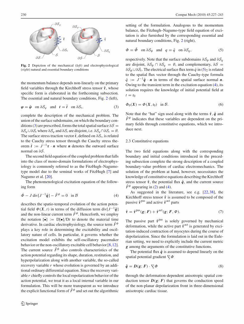
Fig. 2 Depiction of the mechanical (left) and electrophysiological(right) natural and essential boundary conditions

the momentum balance depends non-linearly on the primaryfield variables through the Kirchhoff stress tensor τ , whosespecific form is elaborated in the forthcoming subsection.The essential and natural boundary conditions, Fig. 2 (left),

ϕ = ϕ on ∂Sϕ and t = t on ∂St , (3)

complete the description of the mechanical problem. Theunion of the surface subdomains, on which the boundary con-ditions (3) are prescribed, forms the total spatial surface ∂S =∂Sϕ∪∂St where ∂Sϕ and ∂St are disjoint, i.e. ∂Sϕ∩∂St = ∅.The surface stress traction vector t , defined on ∂St , is relatedto the Cauchy stress tensor through the Cauchy stress the-orem t := J−1τ · n where n denotes the outward surfacenormal on ∂S.

The second field equation of the coupled problem that fallsinto the class of mono-domain formulations of electrophys-iology is commonly referred to as the FitzHugh–Nagumo-type model due to the seminal works of FitzHugh [7] andNagumo et al. [20].

The phenomenological excitation equation of the follow-ing form

Φ − J div[J−1q] − Fφ = 0 in B (4)

describes the spatio-temporal evolution of the action poten-tial field Φ(X, t) in terms of the diffusion term div[J−1q]and the non-linear current term Fφ . Henceforth, we employthe notation ˙[•] := D[•]/Dt to denote the material timederivative. In cardiac electrophysiology, the source term Fφ

plays a key role in determining the excitability and oscil-latory nature of cells. In particular, it governs whether theexcitation model exhibits the self-oscillatory pacemakerbehavior or the non-oscillatory excitable cell behavior [8,12].The current source Fφ also controls characteristics of theaction potential regarding its shape, duration, restitution, andhyperpolarization along with another variable, the so-calledrecovery variable r whose evolution is governed by an addi-tional ordinary differential equation. Since the recovery vari-able r chiefly controls the local repolarization behavior of theaction potential, we treat it as a local internal variable in ourformulation. This will be more transparent as we introducethe explicit functional form of Fφ and set out the algorithmic

setting of the formulation. Analogous to the momentumbalance, the Fitzhugh–Nagumo-type field equation of exci-tation is also furnished by the corresponding essential andnatural boundary conditions, Fig. 2 (right),

Φ = Φ on ∂Sφ and q = q on ∂Sq , (5)

respectively. Note that the surface subdomains ∂Sφ and ∂Sq

are disjoint, ∂Sφ ∩ ∂Sq = ∅, and complementary, ∂S =∂Sφ∪∂St . The electrical surface flux term q in (5)2 is relatedto the spatial flux vector through the Cauchy-type formulaq := J−1q · n in terms of the spatial surface normal n.Owing to the transient term in the excitation equation (4), itssolution requires the knowledge of initial potential field att = t0

Φ0(X) = Φ(X, t0) in B. (6)

Note that the “hat” sign used along with the terms τ , q andFφ indicates that these variables are dependent on the pri-mary fields through constitutive equations, which we intro-duce next.

2.3 Constitutive equations

The two field equations along with the correspondingboundary and initial conditions introduced in the preced-ing subsection complete the strong description of a coupledboundary-value problem of cardiac electromechanics. Thesolution of the problem at hand, however, necessitates theknowledge of constitutive equations describing the Kirchhoffstress tensor τ , the potential flux q, and the current sourceFφ appearing in (2) and (4).

As suggested in the literature, see e.g. [22,38], theKirchhoff stress tensor τ is assumed to be composed of thepassive τ

pas and active τact parts

τ = τpas

(g; F)+ τact

(g; F, Φ). (7)

The passive part τpas is solely governed by mechanical

deformation, while the active part τact is generated by exci-

tation-induced contraction of myocytes during the course ofdepolarization. Since the formulation is laid out in the Eule-rian setting, we need to explicitly include the current metricg among the arguments of the constitutive functions.

The potential flux q is assumed to depend linearly on thespatial potential gradient ∇xΦq = D(g; F) · ∇xΦ (8)

through the deformation-dependent anisotropic spatial con-duction tensor D(g; F) that governs the conduction speedof the non-planar depolarization front in three-dimensionalanisotropic cardiac tissue.

123

Comput Mech (2010) 45:227–243 231

The last constitutive relation describes the electrical sourceterm of the Fitzhugh–Nagumo-type excitation equation (4)

Fφ = Fφe (Φ, r)+ Fφ

m(g; F, Φ) (9)

that is additively decomposed into the excitation-inducedpurely electrical part Fφ

e (Φ, r) and the stretch-induced mec-hano-electrical part Fφ

m(g; F, Φ). The former describes theeffective current generation due to the inward and outwardflow of ions across the cell membrane. This ionic flow istriggered by a perturbation of the resting potential of a car-diac cell beyond some physical threshold upon the arrivalof the depolarization front. The latter, on the other hand,incorporates the opening of ion channels under the action ofdeformation [16,22].

Note that apart from the primary field variables, as webriefly introduced in the preceding subsection, the recov-ery variable r appears among the arguments of Fφ

e in (9). Itdescribes the repolarization response of the action potential.Evolution of the recovery variable r chiefly determines theshape and duration of the action potential locally inherent toeach cardiac cell and may change throughout the heart. Forthis reason, evolution of the recovery variable r is commonlymodeled by a local ordinary differential equation

r = f r (Φ, r). (10)

From an algorithmic point of view, the local nature of theevolution equation (10) allows us to treat the recovery vari-able as an internal variable. This is one of the key features ofthe proposed formulation that preserves the modular globalstructure of the field equations as set out in our recent work[8]. Furthermore, as mentioned in Sect. 1, cardiac tissuepossesses an anisotropic and inhomogeneous micro-struc-ture. This undoubtedly necessitates the explicit incorpora-tion of position-dependent orientation of myocytes, possiblyin terms of structural tensors, in the argument list of the con-stitutive functions for τ , D and Fφ

m . At this stage, however,we have suppressed this dependency for the sake of concise-ness by leaving details out until Sect. 4 where we introducea model problem.

Having the field equations and the functional forms of theconstitutive equations at hand, we are now in a position toconstruct a unified finite element framework for the mono-lithic numerical solution of the strongly coupled problem ofcardiac electromechanics.

3 Finite element formulation

This section is devoted to the construction and consistentlinearization of weak integral forms of the local non-linearfield equations (2) and (4) introduced in the preceding sec-tion. For this purpose, we employ conventional isoparametricspatial discretization for the placement ϕ(X, t) and potential

Φ(X, t) fields to transform the continuous integral equationsfor the non-linear weighted residual and for the Newton-typeupdate to a set of coupled, discrete algebraic equations. Thisset of algebraic equations is then solved monolithically in aniterative manner for the nodal degrees of freedom.

3.1 Weak formulation

We follow the conventional Galerkin procedure to constructthe weak forms of the governing field equations (2) and (4).To this end, we multiply the residual equations by the square-integrable weight functions δϕ ∈ U0 and δΦ ∈ V0 that sat-isfy the essential boundary conditions (3) and (5) such thatδϕ = 0 on ∂Sϕ and δΦ = 0 on ∂Sφ . We then integratethe weighted residual equations over the solid volume, andcarry out integration by parts to obtain the following weightedresidual expressions for the balance of linear momentum (2)

Gϕ(δϕ,ϕ, Φ) = Gϕint(δϕ,ϕ, Φ)− Gϕ

ext(δϕ) = 0 (11)

and for the FitzHugh–Nagumo-type equation (4)

Gφ(δΦ,ϕ, Φ) = Gφint(δΦ,ϕ, Φ)− Gφ

ext(δΦ,ϕ, Φ)=0,

(12)

respectively. Explicit forms of the internal Gϕint and external

Gϕext terms in (11) are separately defined as

Gϕint(δϕ,ϕ, Φ) :=

∫

B∇x (δϕ) : τ dV,

(13)Gϕ

ext(δϕ) :=∫

Bδϕ · B dV +

∫

∂St

δϕ · t da,

where the body force B and the surface traction t are assumedto be given. Likewise, we obtain the following expressionsfor Gφ

int and Gφext

Gφint(δΦ,ϕ, Φ) :=

∫

B(δΦ Φ + ∇x (δΦ) · q) dV,

(14)Gφ

ext(δΦ,ϕ, φ) :=∫

BδΦ FφdV +

∫

∂Sq

δΦ qda,

respectively. The surface flux q is prescribed as a naturalboundary condition through (5)2. Observe that, in contrast tothe mechanical external term in (13)2, Gφ

ext depends explic-itly upon the field variables due to the non-linear source termFφ introduced in (9).

Before proceeding with the consistent linearization of theweak forms, it is convenient to introduce the discretizationof the time space T := [0, t]. For this purpose, we divideup the time interval T into nstp divisions such that T =⋃nstp−1

n=0 [tn, tn+1]. The current time step is denoted with�t := t− tn where we have suppressed the subscript “n+1”

123

232 Comput Mech (2010) 45:227–243

for the sake of compactness. Having the temporal discreti-zation defined, we use the implicit Euler scheme to computethe time derivative of the potential Φ at time t

Φ ≈ (Φ −Φn)/�t (15)

with Φn := Φ(X, tn). Substitution of this finite differenceapproximation for Φ into (14)1 yields the following algorith-mic form

Gφ,algoint (δΦ,ϕ, Φ) =

∫

B( δΦ

Φ −Φn

�t+ ∇x (δΦ) · q ) dV .

(16)

With the weak forms of the field equations at hand, we canthen go on to carry out the consistent linearization.

Remark 1 Since the primary focus of the present formu-lation is the numerical treatment of the strongly coupledcardiac electromechanics; in the weak formulation of themechanical part Gϕ of the coupled problem, we restrict our-selves solely to the displacement approximation. Neverthe-less, a possible extension of the present mechanical settingtoward the well-established three-field (pressure-dilatation-displacement) finite element formulation along with theisochoric–volumetric decomposition of the deformation gra-dient can readily be carried out if quasi-incompressibilityneeds to be accounted for. The incompressibility of myocar-dium, on the other hand, seems to be a rather controversialissue due to the vascular network that constitutes 10–20%of the total volume of the ventricular wall. According to theexperimental results reported by Yin et al. [43], for example,the changes in wall volume range between 5 and 10% due tothe intravascular blood flow.

3.2 Consistent algorithmic linearization

The weighted residual equations (11) and (12) are non-lin-ear functions of the field variables due to the spatial gra-dient operators and the non-linear constitutive equations.Therefore, simultaneous treatment of these equations neces-sitates utilization of Newton-type iterative solution schemeswithin the framework of the implicit finite element method.Accordingly, we carry out the consistent linearization of theweighted residuals with respect to the field variables at anintermediate iteration step at which the field variables assumethe respective values ϕ and Φ to obtain:

Lin Gϕ(δϕ,ϕ, Φ)∣∣ϕ,Φ:= Gϕ(δϕ, ϕ, Φ)

+�Gϕ(δϕ, ϕ, Φ;�ϕ,�Φ) = 0 ,

Lin Gφ(δΦ,ϕ, Φ)∣∣ϕ,Φ:= Gφ(δΦ, ϕ, Φ)

+�Gφ(δΦ, ϕ, Φ;�ϕ,�Φ) = 0.

(17)

The incremental terms �Gϕ and �Gφ , which can beobtained through the Gâteaux derivative, may be expressedin the following decomposed form

�Gγ = �Gγint −�Gγ

ext for γ = ϕ, φ, (18)

based on the definitions in (11) and (12). We then start withthe elaboration of the increment �Gϕ

int according to (13)1

�Gϕint =

∫

B�(∇x (δϕ)) : τ +∇x (δϕ) : �τ dV . (19)

Linearization of the non-linear terms in (19) yields

�(∇x (δϕ)) = −∇x (δϕ)∇x (�ϕ) , (20)

�τ = £�ϕτ +∇x (�ϕ) τ + τ ∇Tx (�ϕ)+ Cϕφ�Φ, (21)

where £�ϕτ denotes the objective Lie derivative along theincrement �ϕ and can be expressed as

£�ϕτ = Cϕϕ : 1

2 £�ϕ g = Cϕϕ : (g∇x (�ϕ)). (22)

in terms of the Lie derivative of the current metric

£�ϕ g = g ∇x (�ϕ)+ ∇Tx (�ϕ) g. (23)

The fourth-order spatial tangent moduli Cϕϕ in (22) and the

sensitivity of the Kirchhoff stresses to the action potentialCϕφ introduced in (21) are defined as

Cϕϕ :=2∂g τ (g; F, Φ) and Cϕφ :=∂Φ τ (g; F, Φ), (24)

respectively. Incorporation of the results (20) and (21) alongwith (22)–(24) in (19) results in the following well-knownexpression

�Gϕint =

∫

B∇x (δϕ) : Cϕϕ : (g∇x (�ϕ))dV

+∫

B∇x (δϕ) : (∇x (�ϕ)τ )dV

+∫

B∇x (δϕ) : Cϕφ�ΦdV . (25)

The three terms on the right-hand side of (25) clearly dem-onstrate the inherent nonlinearities arising from the entirelymechanical material response, from the geometry, and fromthe coupled electromechanical stress response. Since thebody force B and the traction boundary conditions t in (13)2

are prescribed, we have �Gϕext = 0 yielding the identity

�Gϕ ≡ �Gϕint.

Recalling the explicit algorithmic form of Gφint from (16),

the increment �Gφint can be expressed as

�Gφint =

∫

BδΦ

�Φ

�t+�(∇xδΦ) · q +∇x (δΦ) ·�qdV .

(26)

123

Comput Mech (2010) 45:227–243 233

Analogous to (20), linearization of ∇x (δΦ) leads to

�(∇x (δΦ)) = −∇x (δΦ)∇x (�ϕ). (27)

Furthermore, based on the functional definition of the spatialpotential flux q in (8), we obtain

�q = £�ϕ q + ∇x (�ϕ) · q + D · ∇x (�Φ) (28)

where £�ϕ q denotes the Lie derivative of the potential fluxq along the increment �ϕ

£�ϕ q = Cφϕ : 12 £�ϕ g = Cφϕ : (g∇x (�ϕ)). (29)

In Eqs. (28) and (29), we introduced the second-order defor-mation-dependent conduction tensor D and the third-ordermixed moduli Cφϕ that are defined as

D:=∂∇x Φ q(g; F, Φ) and Cφϕ :=2∂g q(g; F, Φ), (30)

respectively. Substituting the results (27) and (28) and thedefinitions (29) and (30) into (26), we end up with

�Gφint =

∫

BδΦ

�Φ

�tdV

+∫

B∇x (δΦ) · D · ∇x (�Φ)dV

+∫

B∇x (δΦ) · Cφϕ : (g∇x (�ϕ))dV . (31)

In contrast to Gϕext, the external term Gφ

ext in (12) dependsnon-linearly on the field variables through the source termFφ(g; F, Φ) introduced in (9). For a given q on ∂Sq , wethen obtain the following incremental form

�Gφext :=

∫

BδΦ �FφdV . (32)

In the Eulerian setting, linearization of the scalar-valued func-tion Fφ yields

�Fφ = H : (g∇x (�ϕ))+ H�Φ (33)

where the tangent terms H and H are defined as

H := 2∂g Fφ(g; F, Φ) and H := ∂Φ Fφ(g; F, Φ), (34)

respectively. Based on the decomposed form introduced in(9), the scalar tangent term H can be expressed as

H = He + Hm with He :=∂Φ Fφe , Hm :=∂Φ Fφ

m. (35)

Inserting the results (33) and (34) into (32), we obtain thelinearized external term

�Gφext =

∫

BδΦ

(H : (g∇x (�ϕ))+ H�Φ

)dV . (36)

This completes the linearization within the continuous spa-tial setting. In the subsequent part, we carry out the spatial

discretization of the field variables to obtain algebraic coun-terparts of the residual expressions (13) and (14).

3.3 Spatial discretization

To approximate the continuous integral equations for theweak forms (11) and (12) derived in the preceding section,we follow the conventional isoparametric Galerkin proce-dure. To this end, we discretize the domain of interest B intoelement subdomains Bh

e such that B ≈ Bh =⋃nele=1 Bh

e withnel denoting the total number of elements. We then interpo-late the field variables and the associated weight functionsover each element domain by introducing the correspondingdiscrete nodal values and C0 shape functions

δϕhe =

nen∑i=1

N iδxei , δΦh

e =nen∑j=1

N jδΦej ,

ϕhe =

nen∑k=1

N k xek, Φh

e =nen∑l=1

NlΦel , (37)

where nen refers to the number of nodes per element. Basedon the discretization (37), the spatial gradient of the weightfunctions read as

∇x (δϕhe ) =

nen∑i=1

δxei ⊗∇x N i ,

∇x (δΦhe ) =

nen∑j=1

δΦej ⊗∇x N j . (38)

Likewise, we obtain the spatial gradient of the incrementalfields

∇x (�ϕhe ) =

nen∑k=1

�xek ⊗∇x N k,

∇x (�Φhe ) =

nen∑l=1

�Φel ⊗∇x Nl . (39)

Incorporating the discretized representations (37) and (38) in(11) and (12) along with (13) and (14), we end up with thediscrete residual vectors

RϕI =Anel

e=1

⎧⎪⎨⎪⎩

∫

Bhe

∇x N i · τ dV

−∫

Bhe

N i B dV −∫

∂Set

N i t da

⎫⎪⎬⎪⎭ = 0,

123

234 Comput Mech (2010) 45:227–243

RφJ =Anel

e=1

⎧⎪⎨⎪⎩

∫

Bhe

(N j Φ −Φn

�t+ ∇x N j · q) dV

−∫

Bhe

N j Fφ dV −∫

∂Seq

N j q da

⎫⎪⎬⎪⎭ = 0, (40)

where the operator A designates the standard assembly ofelement contributions at the local element nodes i, j = 1,

. . . , nen to the global residuals at the global nodes I, J =1, . . . , nnd of a mesh with nnd nodes. Following the analo-gous steps, the discrete form of the linearized residual terms(17) can readily be obtained by substituting the discretizedrepresentations (37) and (39) in (25), (31), and (36). Thisstep, however, is left out for the sake of conciseness.

4 Model problem

In this section, we present specific forms of the constitutiveequations that are utilized in the representative numericalexamples in Sect. 5. In particular, we identify the concreteexpressions for the Kirchhoff stress τ , the potential flux q,and the current source Fφ , whose functional dependencieshave already been briefly outlined in Sect. 2.3. These con-stitutive equations include not only the explicit functionalevaluations but also the accompanying ordinary differen-tial equations governing the temporal evolution of additionalinternal variables. This, in turn, necessitates construction ofalgorithmic procedures for the local update of these inter-nal variables at quadrature points. Hence, the tangent moduliintroduced in Sect. 3.2 have to be computed consistently withthe employed algorithmic integration scheme for the updateof internal variables.

4.1 Active and passive stress response

Before going into the details of the model problem, it is cru-cial to introduce an approach that we devise to account forthe fibrous micro-structure of cardiac tissue in the currentmodel. As mentioned in Sect. 1, cardiac tissue possesses ahighly anisotropic micro-structure that is chiefly made upof unevenly distributed myofibers. This heterogeneous butwell-organized architecture is of fundamental importance forthe successful transduction of essentially one-dimensionalexcitation–contraction of individual cardiac cells to the over-all pumping function of the heart. For this reason, the consti-tutive equations describing the passive and active tissue stressresponse, as well as the one controlling the conductivity, haveto account for the inherently anisotropic micro-structure. Itis the objective of this section to demonstrate that an ele-mentary constitutive approach accounting for basic physical

features of cardiac tissue can reproduce physiological results.For this purpose, we restrict ourselves to transversely isotro-pic cardiac tissue with one single, spatially varying preferreddirection that characterizes the local orientation of myofi-bers. Specifically, we let a0(X) ∈ TXB be a unit vector, i.e.|a0|G = 1, and denote the average preferred direction ofmyofibers in the reference configuration at a material pointX . Under the action of ϕt , this vector is mapped onto itsspatial counterpart a(x) = Fa0 ∈ Tx S emanating fromx = ϕt (X). Moreover, we define the symmetric referencestructural tensor

M(X) := a0 ⊗ a0 (41)

as a key measure of the underlying transversely isotropicmaterial symmetry. Structural tensors are widely employedto develop coordinate-free representation of isotropic ten-sor functions for anisotropic response of materials, see e.g.Spencer [40].

We now assume the following elementary form for thepurely mechanical, passive part of the Kirchhoff stress ten-sor (7)1

τpas

(g; F, M) =(

λ

2ln I3 − µ

)g−1 + µb

+ 2ϑ η(I4 − 1)m (42)

in terms of the inverse metric g−1, the left Cauchy–Greentensor b := FG−1 FT , and the deformed structural tensorm := a⊗ a = FMFT . The Lamé constants λ and µ governthe isotropic stress response, while the parameter η can beconceived as the passive stiffness of myofibers. The aniso-tropic part of the stress is assumed to be active only when thefibers are under tension. This condition is imposed throughthe following conditional definition of the coefficient ϑ

ϑ(λ) ={

1 if λ > 1,

0 otherwise,(43)

where λ := |a|g = √a · ga refers to the stretch in thepreferred direction a. Furthermore, the invariants I3 and I4

appearing in the stress expression (42) are defined as

I3 := J 2 = det(FT g F) and I4 := g : m , (44)

respectively. Observe that the invariant I4 is none other thanthe fiber stretch squared, I4 = λ2.

Since the active Kirchhoff stress τact is generated by exci-

tation-induced contraction of spatially well organized cardiaccells, this part of the stress tensor is considered to be of purelyanisotropic form

τact

(g; F, Φ, M) = σ(Φ) m. (45)

In contrast to recent constitutive equations proposed in theliterature, e.g. [22,25], where the active stress contributionis incorporated as an isotropic function, we assume that the

123

Comput Mech (2010) 45:227–243 235

Fig. 3 Switch function ε(Φ) is plotted against the potential Φ for dif-ferent values of the rate parameter ξ=0.1, 0.2, 0.4, 1 mV−1 and forε0=0.1 ms−1, ε∞=1 ms−1, Φ=− 30 mV

active part is entirely anisotropic. From the geometrical pointof view, the active stress expression (45) implies that thedirection of the active stress tensor is dictated by the deformedstructural tensor m, while its magnitude is chiefly determinedby the transmembrane potential-dependent active fiber ten-sion σ(Φ). To model the twitch-like response of the fibertension σ(Φ), we adopt the evolution equation proposed byNash and Panfilov [22]

σ = ε(Φ)[kσ (Φ −Φr )− σ ] , (46)

where the parameter kσ controls the saturated value of σ

for a given potential Φ and a given resting potential Φr ,which is about−80 mV for cardiac cells. That is, σ vanishesidentically when σ admits the value σ∞ = kσ (Φ − Φr )

for ε(Φ) = 0. Moreover, contrary to its Heaviside form pro-posed in [22], we use the following smoothly varying formfor the rate switch function

ε(Φ) = ε0 + (ε∞ − ε0) exp[− exp(−ξ(Φ − Φ))] (47)

in terms of the parameters ε0 and ε∞ that characterize the twolimiting values of the function for Φ < Φ and Φ > Φ aboutthe phase shift Φ, respectively. In addition, the transition rateof ε from ε0 to ε∞ about Φ is determined by the parameterξ . As depicted in Fig. 3, as the value of ξ gets higher, thetransition of the function ε from ε0 to ε∞ becomes sharper.

In order to compute the current value of σ , we use thebackward Euler scheme. For a typical time step �t = t − tn ,we then obtain

σ = σn +�t ε(Φ)[kσ (Φ −Φr )− σ ]. (48)

This immediately results in a closed-form algorithmic expres-sion for the current value of the active fiber tension

σ(Φ) = 1

1+�t ε(Φ)[σn +�t ε(Φ) kσ (Φ −Φr )] (49)

in terms of the current action potential Φ and σn at time tnthat is stored as a history variable at each quadrature point

of the finite element model. Having the stress expressions athand, we are now in a position to determine the moduli basedon the definition (24)1

Cϕϕ = λ g−1 ⊗ g−1 − (λ ln I3 − 2µ) Ig−1

+ 4ϑ η m ⊗ m (50)

where we have made use of the results ∂g I3 = I3 g−1, ∂g I4 =m. The symmetric fourth identity tensor Ig−1 := −∂g g−1

has the indicial representation Ii jklg−1 := 1

2 (gik g jl + gil g jk)

in terms of the components of the inverse metric gi j . Sim-ilarly, the sensitivity of the Kirchhoff stress tensor to thetransmembrane potential then follows from (24)2

Cϕφ = σ ′(Φ) m with σ ′(Φ) := ∂Φσ(Φ). (51)

Being consistent with the implicit integration schemeemployed in (49), it can be readily shown that

σ ′(Φ) = �t

1+�t ε(Φ)

× [ε′(Φ)(kσ (Φ −Φr )− σ)+ ε(Φ) kσ

], (52)

where the derivative ε′(Φ) := ∂Φε(Φ) can be obtained fromthe definition (47)

ε′(Φ) = ξ (ε(Φ)− ε0) exp[−ξ(Φ − Φ)]. (53)

4.2 Spatial potential flux

We have already introduced the spatial potential flux q in (8)in terms of the conduction tensor D (30)1, and the potentialgradient ∇xΦ. In this model problem, the second-order con-duction tensor is additively decomposed into the isotropicand anisotropic parts

D = diso g−1 + dani m (54)

in terms of the scalar conduction coefficients diso and dani,where the latter accounts for the faster conduction along themyofiber directions. Having D specified, we can express thethird-order mixed moduli Cφϕ based on their definition givenin (30)2

Cφϕ = −2 diso∇xΦ · Ig−1 . (55)

4.3 Current source

In order to complete the description of the model problem,we finally need to specify the constitutive equations for theelectrical source term Fφ . In the field of phenomenologicalelectrophysiology, it is common practice to set up the modelequations and parameters in the non-dimensional space. Forthis purpose, we introduce the non-dimensional transmem-brane potential φ and the non-dimensional time τ through

123

236 Comput Mech (2010) 45:227–243

the following conversion formulae

Φ = βφφ − δφ and t = βtτ. (56)

The non-dimensional potential φ is related to the phys-ical transmembrane potential Φ through the factor βφ andthe potential difference δφ , which are both in millivolt (mV).Likewise, the dimensionless time τ is converted to the phys-ical time t by multiplying it with the factor βt in millisecond(ms). Having the basic relations (56) at hand, we obtain thefollowing conversion expressions

Fφ = βφ

βtf φ, H = βφ

βth and H = 1

βth (57)

for the normalized source term f φ , and the non-dimensionalcounterparts h := ∂φ f φ and h := 2∂g f φ of the tangent

terms defined in (34). The additive split of Fφ , introduced in(9) Sect. 2.3, along with (57)1 implies the equivalent decom-position of f φ = f φ

e + f φm into the purely electrical part

f φe and the stretch-induced mechano-electrical part f φ

m. Thisalso leads to the dimensionless counterpart of (35)

h = he + hm with he := ∂φ f φe , hm := ∂φ f φ

m . (58)

In this model problem, we use the celebrated Aliev–Panfilovmodel, which favorably captures the characteristic shape ofthe action potential in excitable ventricular cells,

f φe = cφ(φ − α)(1− φ)− r φ (59)

where c, α are material parameters. The evolution of therecovery variable r is governed by the ordinary differentialequation (10) through the specific source term

f r =[γ + µ1 r

µ2 + φ

][−r − c φ (φ − b − 1)]. (60)

The coefficient term [γ + µ1r/µ2 + φ] plays a key role incontrolling the restitution characteristics of the modelthrough the additional material parameters µ1, µ2, b and γ .The phase diagram in Fig. 4 (top) depicts the solution trajec-tories of the local ordinary differential equations ∂τφ = f φ

e

and ∂τ r = f r corresponding to different initial points φ0 andr0. Note that the dashed nullclines, where f φ = 0 or f r = 0vanish, guide the trajectories. The diagrams in Fig. 4 (bot-tom) show the non-dimensional potential φ and the recoveryvariable r curves plotted against the dimensionless time τ .The action potential is generated by adding external stimula-tion I = 30 to the right-hand side of ∂τφ = f φ

e from τ = 30to τ = 30.02.

Analogous to the algorithmic update of σ , we use thebackward Euler integration to calculate the current value ofr . Owing to the highly non-linear form of the source f r ,however, we need to introduce the residual

Rr = r − rn −�τ f r (φ, r).= 0 (61)

Fig. 4 The Aliev–Panfilov model with α = 0.01, γ = 0.002,

b = 0.15, c = 8, µ1 = 0.2, µ2 = 0.3. The phase portrait depictstrajectories for distinct initial values φ0 and r0 (filled circles) converg-ing to a stable equilibrium point (top). Non-oscillatory normalized timeplot of the non-dimensional action potential φ and the recovery variabler (bottom)

that has to be solved iteratively. Linearization of (61) leadsus to the local update equation of the recovery variable r

r ← r − (Crr )−1 Rr , (62)

where the scalar local tangent Crr is defined by

Crr := ∂r Rr

= 1+�τ

[γ + µ1

µ2 + φ[2r + cφ(φ − b − 1)]

].

(63)

Calculation of the modulus he, defined in (58)2, necessitatesthe knowledge of the derivative of the recovery variable rwith respect to the action potential φ. This derivative canbe calculated based on the persistency condition dφ Rr =∂φ Rr + ∂r Rr dφr

.= 0, which implies the consistent ful-fillment of (61) throughout the whole calculation. Solvingthis equality for the sought derivative, we obtain dφr =

123

Comput Mech (2010) 45:227–243 237

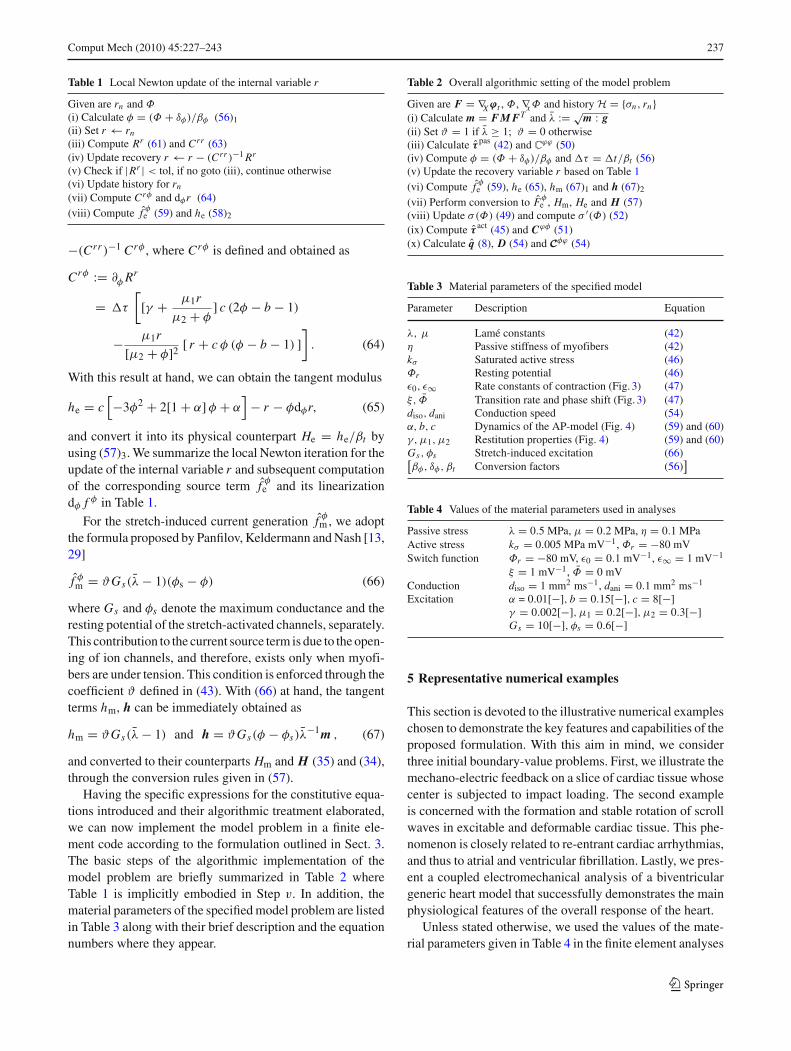
Table 1 Local Newton update of the internal variable r

Given are rn and Φ

(i) Calculate φ = (Φ + δφ)/βφ (56)1(ii) Set r ← rn(iii) Compute Rr (61) and Crr (63)(iv) Update recovery r ← r − (Crr )−1 Rr

(v) Check if |Rr | < tol, if no goto (iii), continue otherwise(vi) Update history for rn

(vii) Compute Crφ and dφr (64)(viii) Compute f φ

e (59) and he (58)2

−(Crr )−1 Crφ , where Crφ is defined and obtained as

Crφ := ∂φ Rr

= �τ

[[γ + µ1r

µ2 + φ] c (2φ − b − 1)

− µ1r

[µ2 + φ]2 [ r + c φ (φ − b − 1) ]]

. (64)

With this result at hand, we can obtain the tangent modulus

he = c[−3φ2 + 2[1+ α]φ + α

]− r − φdφr, (65)

and convert it into its physical counterpart He = he/βt byusing (57)3. We summarize the local Newton iteration for theupdate of the internal variable r and subsequent computationof the corresponding source term f φ

e and its linearizationdφ f φ in Table 1.

For the stretch-induced current generation f φm, we adopt

the formula proposed by Panfilov, Keldermann and Nash [13,29]

f φm = ϑGs(λ− 1)(φs − φ) (66)

where Gs and φs denote the maximum conductance and theresting potential of the stretch-activated channels, separately.This contribution to the current source term is due to the open-ing of ion channels, and therefore, exists only when myofi-bers are under tension. This condition is enforced through thecoefficient ϑ defined in (43). With (66) at hand, the tangentterms hm, h can be immediately obtained as

hm = ϑGs(λ− 1) and h = ϑGs(φ − φs)λ−1m , (67)

and converted to their counterparts Hm and H (35) and (34),through the conversion rules given in (57).

Having the specific expressions for the constitutive equa-tions introduced and their algorithmic treatment elaborated,we can now implement the model problem in a finite ele-ment code according to the formulation outlined in Sect. 3.The basic steps of the algorithmic implementation of themodel problem are briefly summarized in Table 2 whereTable 1 is implicitly embodied in Step v. In addition, thematerial parameters of the specified model problem are listedin Table 3 along with their brief description and the equationnumbers where they appear.

Table 2 Overall algorithmic setting of the model problem

Given are F = ∇X ϕt , Φ, ∇xΦ and history H = {σn, rn}(i) Calculate m = F M FT and λ := √m : g(ii) Set ϑ = 1 if λ ≥ 1; ϑ = 0 otherwise(iii) Calculate τ

pas (42) and Cϕϕ (50)

(iv) Compute φ = (Φ + δφ)/βφ and �τ = �t/βt (56)(v) Update the recovery variable r based on Table 1(vi) Compute f φ

e (59), he (65), hm (67)1 and h (67)2

(vii) Perform conversion to Fφe , Hm, He and H (57)

(viii) Update σ(Φ) (49) and compute σ ′(Φ) (52)(ix) Compute τ

act (45) and Cϕφ (51)(x) Calculate q (8), D (54) and Cφϕ (54)

Table 3 Material parameters of the specified model

Parameter Description Equation

λ, µ Lamé constants (42)η Passive stiffness of myofibers (42)kσ Saturated active stress (46)Φr Resting potential (46)ε0, ε∞ Rate constants of contraction (Fig. 3) (47)ξ, Φ Transition rate and phase shift (Fig. 3) (47)diso, dani Conduction speed (54)α, b, c Dynamics of the AP-model (Fig. 4) (59) and (60)γ, µ1, µ2 Restitution properties (Fig. 4) (59) and (60)Gs , φs Stretch-induced excitation (66)[βφ, δφ, βt Conversion factors (56)

]

Table 4 Values of the material parameters used in analyses

Passive stress λ = 0.5 MPa, µ = 0.2 MPa, η = 0.1 MPaActive stress kσ = 0.005 MPa mV−1, Φr = −80 mVSwitch function Φr = −80 mV, ε0 = 0.1 mV−1, ε∞ = 1 mV−1

ξ = 1 mV−1, Φ = 0 mVConduction diso = 1 mm2 ms−1, dani = 0.1 mm2 ms−1

Excitation α = 0.01[−], b = 0.15[−], c = 8[−]γ = 0.002[−], µ1 = 0.2[−], µ2 = 0.3[−]Gs = 10[−], φs = 0.6[−]

5 Representative numerical examples

This section is devoted to the illustrative numerical exampleschosen to demonstrate the key features and capabilities of theproposed formulation. With this aim in mind, we considerthree initial boundary-value problems. First, we illustrate themechano-electric feedback on a slice of cardiac tissue whosecenter is subjected to impact loading. The second exampleis concerned with the formation and stable rotation of scrollwaves in excitable and deformable cardiac tissue. This phe-nomenon is closely related to re-entrant cardiac arrhythmias,and thus to atrial and ventricular fibrillation. Lastly, we pres-ent a coupled electromechanical analysis of a biventriculargeneric heart model that successfully demonstrates the mainphysiological features of the overall response of the heart.

Unless stated otherwise, we used the values of the mate-rial parameters given in Table 4 in the finite element analyses

123

238 Comput Mech (2010) 45:227–243

of the examples presented in this section. Observe that theparameters belonging to the Aliev–Panfilov model f φ

e andto the stretch-induced part of the excitation source f φ

m aredimensionless. This is consistent with the non-dimensionalsetting introduced through the conversion formulae (56) and(57). In the conversion, we employ the factors βφ = 100 mV,δφ = −80 mV and βt = 12.9 ms that are chosen to obtain thephysiological action potential response ranging from−80 to+20 mV and the characteristic action potential duration, assuggested in [1].

5.1 Deformation-induced excitation of cardiac tissue

In order to illustrate the phenomenon of mechano-electricfeedback, we consider a three-dimensional 100mm×100mm× 12 mm slice of cardiac tissue, see the upper leftmost panelin Fig. 6 for dimensioning. The tissue block is discretized into21×21×2 eight-node coupled brick elements. The myofibersare assumed to be oriented in x−direction, i.e. a0 = e1, withrespect to the global coordinate system depicted in Fig. 5.Initial value of the transmembrane potential in the wholedomain is set to its resting value Φ(X, t0) = −80 mV. Thedisplacement degrees of freedom in the z-direction at the

nodes located on the four edges of the mid-plane (z = 6)

of the slice are restrained. Moreover, the displacements inthe x- and y-directions at (0, 0, 0) and the displacement inthe y-direction at the node located at (100, 0, 0) are fixed.Furthermore, the outer surface of the tissue is assumed tobe electrically insulated, i.e. q = 0 on ∂S. In order to ini-tiate the excitation, the nodes located within the central,20 mm × 20 mm × 12 mm, parallelepiped are subjected toimpulsive cyclic loading p(t) in z-direction, see the upperleftmost panel Fig. 5. The loading p(t) is increased propor-tionally up to 1 N within the first 5 ms and then decreased backto the zero load level at the same rate. The snapshot taken att = 5 ms in Fig. 5 demonstrates the deformed shape of thetissue at the instant of peak loading. Besides the deformedshapes, the contour plots of action potential are also depictedat each snapshot.

The impulsive loading in the transverse direction givesrise to the tension-dominated deformation in the center ofthe tissue. This region then undergoes the stretch-inducedexcitation through the activation of ion channels due to thesource term Fφ

m introduced in (9) and (66) as depicted inthe panel at t = 10 ms in Fig. 5. The excitation leads todepolarization of the tissue from the center, and in turn, exci-

Fig. 5 Deformation-induced excitation of deformable cardiac tissue.Snapshots of the deformed model depict the action potential contours atdifferent stages of depolarization (upper row) and repolarization (lower

row). Note that the cardiac tissue recovers its original shape at t = 0 msupon completion of repolarization at t ≈ 360 ms

123

Comput Mech (2010) 45:227–243 239

Fig. 6 Initiation and rotation of scroll re-entry in excitable and deformable cardiac tissue. The re-entrant scroll is triggered by externally stimulatingtail of the repolarization wave through the addition of I = 5 to f φ

e from 440 to 460 ms at the rectangular region

tation-induced contraction of myofibers that are located inthe x-direction, see the snapshot at t = 30 ms. Both the con-traction of myofibers and the higher rate of conduction in thex-direction result in faster depolarization along that direc-tion. This non-uniform deformation pattern brings about thebending of the slice, thereby triggering secondary excita-tion at the upper and lower edges of the domain, as shownin the panel corresponding to t = 55 ms. The two depo-larization fronts then merge, and cause the whole tissue tobecome completely depolarized, see the panel at t = 80 ms.The snapshots taken at t = 280, 300, 330 ms illustrate thesequence of tissue repolarization from the excited state withΦ = +20 mV back to the resting state with Φ = −80 mV.The repolarization process is also accompanied by the relaxa-tion of myocytes leading to the recovery of the original shapeat around t = 360 ms.

5.2 Scroll waves in a slice of cardiac tissue

One of the key benchmark problems of computational cardiacelectrophysiology and electromechanics is the simulation ofthree-dimensional scroll waves. These re-entrant waves areclosely related to cardiac arrhythmias, such as atrial and ven-

tricular fibrillation. Re-entry may arise from different inho-mogeneities such as the uneven distribution of conductionproperties in diseased tissue as in the case of unidirectionalblock or unsynchronized multiple pacemakers.

In order to simulate the re-entrant waves in deformablecardiac tissue, we devise the same geometry and discretiza-tion as the one used in the preceding boundary-value prob-lem, see the panel at t = 3 ms in Fig. 6. The values of thematerial parameters are selected to be the same as in Table 4except that Gs = 0 such that mechano-electric feedbackeffect is suppressed. To generate a scroll wave, we followthe conventional procedure suggested in [8,9]. To this end,we initiate a planar depolarization front in x-direction byassigning elevated initial values to the nodal action potentialsΦ0 = −40 mV on the plane located at x = 0 mm. The initialvalue of the nodal transmembrane potential at the remain-der of the nodes is set to the resting value Φ0 = −80 mV.The outer surface of the tissue is assumed to be electricallyflux-free. Moreover, the orientation of contractile myofibersis assumed to be a0 = e1 with respect to the global coor-dinate system depicted in Fig. 6. In contrast to the mechan-ical essential boundary conditions utilized in the precedingexample, no degree of freedom is a priori prescribed here.

123

240 Comput Mech (2010) 45:227–243

Instead, the nodes on the plane situated at z = 0 are sup-ported by uncoupled linear springs of directional stiffness-es kx = ky = 10−3 N/mm and kz = 10−1 N/mm. Thishas resulted in a system of equations that is stable enoughto tackle, while at the same time, providing a fairly uncon-strained representation of deformed configurations.

Once the wave front has formed, it starts to travel in x-direction, thereby depolarizing the whole domain and lead-ing to contraction of myocytes, see the panel at t = 75 ms inFig. 6. The myocytes then start to relax in the region where therepolarization tail has taken over, as shown in the snapshot att = 420 ms. To initiate the spiral wave re-entry, we externallystimulate the rectangular region bounded by the coordinatesx ∈ [40, 50] mm, y ∈ [0, 55] mm and z ∈ [0, 12] mm withrespect to the initial configuration. The rectangular region isdepolarized by adding the extra current I = 5 to f φ

e at timet = 440 ms for 20 ms. Observe that the snapshots corre-sponding to the time steps following the stimulation clearlydemonstrate the stages of initiation, development, and stablerotation of the scroll wave re-entry.

It is important to note that, contrary to the purely electro-physiology-based simulations of re-entrant waves on regulardomains, the center of the scroll does not remain station-ary but drifts due to the deformation, see also [30]. Anothercrucial observation concerns the substantial reduction of theaction potential duration once the scroll wave is initiated.This is closely related to the restitution property of cardiaccells that are able to adjust the action potential duration adap-tively depending upon the frequency of excitation. This fea-ture is well captured by the Aliev–Panfilov model through thenon-linear coefficient term in (60) as discussed extensivelyin [1,8].

5.3 Excitation–contraction of a generic heart model

The key motivation for this work is its potential applicationin guiding stem cell-based therapies in heart failure. As a firstattempt towards this objective, we carry out a three-dimen-sional coupled electromechanical analysis of a biventricu-lar generic heart model and show that basic features of theheart function can be captured by our model. The solid modelof a biventricular generic heart is constructed by means oftwo truncated ellipsoids as suggested in [39]. The genericheart model whose dimensions and spatial discretization aredepicted in Fig. 7 is meshed with 13,348 four-node coupledtetrahedral elements connected at 3,059 nodes. The unevenlydistributed average orientation of contractile myocytes a0 isdepicted with yellow lines in Fig. 8. This fiber organiza-tion is consistent with the myofiber orientation in the humanheart where the fiber angle ranges from approximately−70◦in the epicardium to +70◦ in the endocardium with respectto the z-plane. Displacement degrees of freedom on the topbase surface (z = 0) are restrained and the whole surface of

Fig. 7 Geometry and discretization of a generic heart model generatedby truncated ellipsoids. Dimensions are in millimeters

the heart is assumed to be flux-free. Moreover, we use thesame values of the material parameters as in the precedingexample.

To initiate the excitation, the elevated initial value Φ0 =−10 mV of the transmembrane potential is assigned to thenodes located at the upper part of the septum (wall separat-ing the ventricles) as indicated by the partially depolarizedregion in the panel at t = 3 ms in Fig. 8. The initial trans-membrane potential at the remaining nodes is set to the rest-ing value Φ0 = −80 mV. The excitation at the top of theseptum generates the depolarization front travelling from thelocation of stimulation throughout the entire heart, therebyresulting in the contraction of the myocytes, see the snap-shots taken at t = 75, 105, 135 ms in Fig. 8. At first glance,we observe that the contraction of myocytes gives rise to theupward motion of the apex (bottom part of the heart). Moreimportantly, we also note that the upward motion of the apexis accompanied by the physiologically observed wall thick-ening and the overall torsional motion of the heart. Theseeffects can be better appreciated by looking at the deforma-tion of the two slices presented in the complementary imagesshown in Fig. 9. Undoubtedly, it is the inhomogeneous dis-tribution of myocyte orientation, which is incorporated inthe model both spatially over the surfaces and across thetransmural direction of the ventricular walls, that yields thisphysiological response through the non-uniform contractionof myofibers. The panels in the lower rows of Figs. 8 and 9depict the relaxation of the heart during the course of repo-larization. At the end of the repolarization process, the ref-erence configuration of the heart is fully recovered. Notethat the repolarization starts from regions which depolarizedlast. This is in accordance with the uneven action potentialduration distribution throughout the myocardium where the

123

Comput Mech (2010) 45:227–243 241

Fig. 8 Coupled excitation-induced contraction of generic heart model. Snapshots of the deformed model depict the action potential con-tours at different stages of depolarization (upper row) and repolarization (lower row). The lines denote the spatial orientation a of contractilemyofibers

Fig. 9 Coupled excitation-induced contraction of the generic heartmodel. Snapshots of two slices located at x = 0 and z = 25 mm(Fig. 7) in the three-dimensional model favorably illustrate the phys-

iological wall thickening and overall torsional motion of the heart atdifferent stages of depolarization (upper row) and repolarization (lowerrow)

action potential lasts longer in the endocardial cells than inthe epicardial cells [19]. In the present model, this is achievedby altering the temporal converting factor βt inversely pro-

portional to the excitation time as originally proposed inour recent work on computational modeling of electrocar-diograms [17].

123

242 Comput Mech (2010) 45:227–243

6 Concluding remarks

In this manuscript, we have proposed a new, fully implicit,entirely finite element-based numerical approach to thestrongly coupled non-linear problem of cardiac electrome-chanics. The suggested unified algorithmic formulation hasbeen thoroughly set out by giving full particulars of the weakformulation, consistent linearization, and discretization. Thishas resulted in an unconditionally stable scheme and a mod-ular framework that can readily be extended towards moredetailed constitutive approaches. The particular constitutivemodel considered in this paper accounts for a two-waycoupling; that is, both the excitation-induced contraction ofcardiac tissue and the deformation-induced generation ofexcitation have been incorporated. Apart from theintrinsic coupling, the inherent anisotropic micro-structure ofcardiac tissue is reflected in the model by means of the mod-ern notions of coordinate-free representation of anisotropy interms of structural tensors. This concerns not only the passiveand active non-linear stress response but also the deforma-tion-dependent conduction tensor. The outstanding perfor-mance of the proposed approach has been then demonstratedby means of the three-dimensional benchmark problems thatinclude the re-entrant scroll dynamics and impact loading-generated excitation in the contractile cardiac tissue and thecomplete coupled electromechanical analysis of a biventric-ular generic heart model. It is important to emphasize thatthe fully implicit unified finite element setting allowed usto carry out the benchmark computations with a consider-ably less computational effort compared to the calculationsreported in the literature, which require much finer temporaland spatial discretization.

Acknowledgments This material is based on work supported by theNational Science Foundation under Grant No. EFRI-CBE 0735551Engineering of cardiovascular cellular interfaces and tissue constructs.

References

1. Aliev RR, Panfilov AV (1996) A simple two-variable model of car-diac excitation. Chaos, Solitons Fractals 7:293–301

2. Beeler GW, Reuter H (1977) Reconstruction of the action potentialof ventricular myocardial fibres. J Physiol 268:177–210

3. Bers DM (2002) Cardiac excitationcontraction coupling. Nature415:198–205

4. Clayton RH, Panfilov AV (2008) A guide to modelling car-diac electrical activity in anatomically detailed ventricles. ProgrBiophys Mol Biol 96:19–43

5. Fenton F, Karma A (1998) Vortex dynamics in three-dimensionalcontinuous myocardium with fiber rotation: filament instability andfibrillation. Chaos Interdiscipl J Nonlinear Sci 8:20–27

6. Fenton FH, Cherry EM, Hastings HM, Evans SJ (2002) Multiplemechanisms of spiral wave breakup in a model of cardiac electricalactivity. Chaos Interdiscipl J Nonlinear Sci 12:852–892

7. Fitzhugh R (1961) Impulses and physiological states in theoreticalmodels of nerve induction. Biophys J 1:455–466

8. Göktepe S, Kuhl E (2009) Computational modeling of cardiacelectrophysiology: A novel finite element approach. Int J NumerMethods Eng 79:156–178

9. Göktepe S, Wong J, Kuhl E (2009) Atrial and ventricular fibrilla-tion—computational simulation of spiral waves in cardiac tissue.Arch Appl Mech. doi:10.1007/s00419-009-0384-0

10. Hodgkin A, Huxley A (1952) A quantitative description of mem-brane current and its application to excitation and conduction innerve. J Physiol 117:500–544

11. Holzapfel GA, Ogden RW (2009) Constitutive modelling of pas-sive myocardium: a structurally based framework for materialcharacterization. Phil Trans Ser A, Math Phys Eng Sci367(1902):3445–3475. PMID: 19657007

12. Keener JP, Sneyd J (1998) Mathematical physiology. Springer,New York

13. Keldermann R, Nash M, Panfilov A (2007) Pacemakers in a reac-tion–diffusion mechanics system. J Stat Phys 128:375–392

14. Kerckhoffs R, Healy S, Usyk T, McCulloch A (2006) Compu-tational methods for cardiac electromechanics. Proc IEEE 94:769–783

15. Klabunde RE (2005) Cardiovascular physiology concepts. Lippin-cott Williams & Wilkins, Philadelphia

16. Kohl P, Hunter P, Noble D (1999) Stretch-induced changes in heartrate and rhythm: Clinical observations, experiments and mathemat-ical models. Progr Biophys Mol Biol 71:91–138

17. Kotikanyadanam M, Göktepe S, Kuhl E (2009) Computationalmodeling of electrocardiograms: a finite element approach towardscardiac excitation. Commun Numer Methods Eng. doi:10.1002/cnm.1273

18. Luo CH, Rudy Y (1991) A model of the ventricular cardiac actionpotential. depolarization, repolarization, and their interaction. CircRes 68:1501–1526

19. Malmivuo J, Plonsey R (1995) Bioelectromagnetism. OxfordUniversity Press, Oxford

20. Nagumo J, Arimoto S, Yoshizawa S (1962) An active pulse trans-mission line simulating nerve axon. Proc IRE 50:2061–2070

21. Nash MP, Hunter PJ (2000) Computational mechanics of the heartfrom tissue structure to ventricular function. J Elast 61:113–141

22. Nash MP, Panfilov AV (2004) Electromechanical model of excit-able tissue to study reentrant cardiac arrhythmias. Progr BiophysMol Biol 85:501–522

23. Nickerson D, Nash M, Nielsen P, Smith N, Hunter P (2006) Com-putational multiscale modeling in the IUPS physiome project: mod-eling cardiac electromechanics. IBM J Res Dev 50:617–630

24. Nickerson D, Smith N, Hunter P (2005) New developments ina strongly coupled cardiac electromechanical model. Europace7:S118–127

25. Niederer SA, Smith NP (2008) An improved numerical method forstrong coupling of excitation and contraction models in the heart.Progr Biophys Mol Biol 96:90–111

26. Nielsen PM, Grice IJL, Smaill BH, Hunter PJ (1991) Mathemat-ical model of geometry and fibrous structure of the heart. Am JPhysiol 260:H1365–1378

27. Noble D (1962) A modification of the Hodgkin–Huxley equationsapplicable to purkinje fibre action and pacemaker potentials. JPhysiol 160:317–352

28. Opie LH (2004) Heart physiology: from cell to circulation.Lippincott Williams & Wilkins, Philadelphia

29. Panfilov AV, Keldermann RH, Nash MP (2005) Self-organizedpacemakers in a coupled reaction-diffusion-mechanics system.Phys Rev Lett 95:258,104–1–258,014–4. PMID: 16384515

30. Panfilov AV, Keldermann RH, Nash MP (2007) Drift and breakupof spiral waves in reaction diffusion mechanics systems. Proc NatlAcad Sci 104:7922–7926

31. Plank G, Burton RA, Hales P, Bishop M, Mansoori T, BernabeuMO, Garny A, Prassl AJ, Bollensdorff C, Mason F, Mahmood F,

123

Comput Mech (2010) 45:227–243 243

Rodriguez B, Grau V, Schneider JE, Gavaghan D, Kohl P(2009) Generation of histo-anatomically representative models ofthe individual heart: tools and application. Phil Trans R Soc A367:2257–2292

32. Pope AJ, Sands GB, Smaill BH, LeGrice IJ (2008) Three-dimen-sional transmural organization of perimysial collagen in the heart.Am J Physiol Heart Circ Physiol 295(3):H1243–1252

33. Pullan AJ, Buist ML, Cheng LK (2005) Mathematical modelingthe electrical activity of the heart. World Scientific, Singapore

34. Rogers JM (2002) Wave front fragmentation due to ventriculargeometry in a model of the rabbit heart. Chaos (Woodbury, N.Y.)12:779–787. PMID: 12779606

35. Rogers JM, McCulloch AD (1994) Nonuniform muscle fiber ori-entation causes spiral wave drift in a finite element model of cardiacaction potential propagation. J Cardiovasc Electrophysiol 5:496–509

36. Rohmer D, Sitek A, Gullberg GT (2007) Reconstruction and visu-alization of fiber and laminar structure in the normal humanheart from ex vivo diffusion tensor magnetic resonance imaging(DTMRI) data. Invest Radiol 42:777–789

37. Sachse FB (2004) Computational cardiology: modeling ofAnatomy, electrophysiology, and mechanics. Springer, Berlin

38. Sainte-Marie J, Chapelle D, Cimrman R, Sorine M (2006) Mod-eling and estimation of the cardiac electromechanical activity.Comput Struct 84:1743–1759

39. Sermesant M, Rhode K, Sanchez-Ortiz G, Camara O, Andrian-tsimiavona R, Hegde S, Rueckert D, Lambiase P, Bucknall C,Rosenthal E, Delingette H, Hill D, Ayache N, Razavi R (2005) Sim-ulation of cardiac pathologies using an electromechanical biven-tricular model and XMR interventional imaging. Med Image Anal9:467–480

40. Spencer AJM (1971) Theory of invariants. In: Eringen A (ed)Continuum Physics, vol 1. Academic Press, New York

41. Tusscher KHWJT, Panfilov AV (2008) Modelling of the ventricu-lar conduction system. Progr Biophys Mol Biol 96:152–170

42. Usyk TP, LeGrice IJ, McCulloch AD (2002) Computational modelof three-dimensional cardiac electromechanics. Comput Vis Sci4:249–257

43. Yin FC, Chan CC, Judd RM (1996) Compressibility of per-fused passive myocardium. Am J Physiol Heart Circ Physiol271(5):H1864–1870

44. Zheng Z, Croft J, Giles W, Mensah G (2001) Sudden cardiac deathin the United States. Circulation 104:2158–2163

123