elements of mechanical engineering - …airwalkbooks.com/images/pdf/pdf_56_1.pdf · (vi) propped...

(For B.E./B.Tech Engineering Students)

As per New Revised Syllabus ofDr. APJ Abdul Kalam Technical University - UP

AIRWALK PUBLICATIONS

(Near All India Radio)

80, Karneeshwarar Koil Street

Mylapore, Chennai - 600 004.

Ph.: 2466 1909, 94440 81904

Email: [email protected],

[email protected]

www.airwalkbooks.com

Dr. S. Ramachandran, M.E., Ph.D.,

ELEMENTS OFMECHANICAL ENGINEERING

Saswath Kumar Das,HOD - Mechanical Engineering

Dr. D.R. Somashekar, M.E., Ph.D

DirectorIIMT College of Engineering,

GREATER NOIDA - 201308 (UP)

thFirst Edition: 9 August 2017

ISBN : 978-93-84893-76-7

Price :

ISBN:978-93-84893-76-7

www.airwalkbooks.com

ELEMENTS OF MECHANICAL ENGINEERING

UNIT-I:

Force System: Force, Parallelogram Law, Lami’s theorem, Principle of

Transmissibility of forces. Moment of a force, Couple, Varignon’s theorem,

Resolution of a force into a force and a couple. Resultant of coplanar force

system. Equilibrium of coplanar force system, Free body diagrams,

Determination of reactions. Concept of Centre of Gravity and Centroidand

Area Moment of Inertia, Perpendicular axis theorem and Parallel axis theorem

UNIT-II:

Plane Truss: Perfect and imperfect truss, Assumptions and Analysis of Plane

Truss by Method of joints and Method of section.

Beams: Types of beams, Statically Determinate Beams, Shear force and

bending moment in beams, Shear force and bending moment diagrams,

Relationships between load, shear and bending moment.

UNIT-III:

Simple stress and strain: Normal and shear stresses. One Dimensional

Loading; members of varying cross section, bars in series. Tensile Test

diagram for ductile and brittle materials, Elastic constants, Strain energy.

Bending (Flexural) Stresses: Theory of pure bending, neutral surface and

neutral axis, stresses in beams of different cross sections. Engineering

Materials: Importance of engineering materials, classification, mechanical

properties and applications of Ferrous, Nonferrous and composite materials.

UNI-IV:

Basic Concepts and Definitions of Thermodynamics: Introduction and

definition of thermodynamics, Microscopic and Macroscopic approaches,

System, surrounding and universe, Concept of continuum, Thermodynamic

equilibrium, Thermodynamic properties, path, process and cycle, Quasi static

process, Energy and its forms, Work and heat. Thermodynamic definition of

work.

Syllabus S.1

Zeroth law of thermodynamics: Temperature and its’ measurement.

First law of thermodynamics: First law of thermodynamics, Internal energy

and enthalpy. First law analysis for non-flow processes.

Non-flow work Steady flow energy equation; Boilers, Condensers, Turbine,

Throttling process, Pumps etc.

UNIT-V:

Second law: Thermal reservoir, Kelvin Planck statement, Heat engines,

Efficiency; Clausius’ statement Heat pump, refrigerator, Coefficient of

Performance. Carnot cycle, Carnot theorem and it’s corollaries.Clausius

inequality, Concept of Entropy.

Properties of pure substances: P-v, T-s and h-s diagram, dryness fraction

and steam tables. Rankine Cycle.

Internal Combustion Engines: Classification of I.C. Engines and their parts,

working principle and comparison between 2 Stroke and 4 stroke engine ,

difference between SI and CI engines. Pv and T-s diagramsof Otto and Diesel

cycles, comparison of efficiency.

S.2 Elements of Mechanical Engineering www.airwalkpublications.com

Contents

Chapter 1

Force System - Centroid and Moment of Inertia

1.1 Engineering Mechanics . . . . . . . . . . . . . . . . . . . . . . . . . . . . . . . . . . . . . 1.1

1.2 Classification of Engineering Mechanics . . . . . . . . . . . . . . . . . . . . . . 1.2

1.3 Fundamental Concepts of Mechanics . . . . . . . . . . . . . . . . . . . . . . . . . 1.3

1.4 Scalar and Vector Quantities . . . . . . . . . . . . . . . . . . . . . . . . . . . . . . . . 1.4

1.5 Laws of Mechanics . . . . . . . . . . . . . . . . . . . . . . . . . . . . . . . . . . . . . . . . 1.5

1.5.1 Newton’s Three Fundamental Laws . . . . . . . . . . . . . . . . . . . . 1.5

1.5.2 Newton’s Law of Gravitation . . . . . . . . . . . . . . . . . . . . . . . . . 1.6

1.5.3 The Parallelogram Law of Forces . . . . . . . . . . . . . . . . . . . . . 1.7

1.5.4 Triangular Law of Forces . . . . . . . . . . . . . . . . . . . . . . . . . . . . 1.8

1.5.5 Polygon Law of Forces . . . . . . . . . . . . . . . . . . . . . . . . . . . . . . 1.9

1.5.6 Law (or) Principle of Transmissibility of Forces . . . . . . . . 1.10

1.6 Force and Force System . . . . . . . . . . . . . . . . . . . . . . . . . . . . . . . . . . . 1.11

1.6.1 Types of forces . . . . . . . . . . . . . . . . . . . . . . . . . . . . . . . . . . . . 1.12

1.6.2 Types of force system . . . . . . . . . . . . . . . . . . . . . . . . . . . . . . 1.13

(I) Coplanar force system . . . . . . . . . . . . . . . . . . . . . . . . . . . . . . . . . . 1.14

(a) Concurrent forces . . . . . . . . . . . . . . . . . . . . . . . . . . . . . . . . . . . . . . 1.14

(b) Coplanar - concurrent force system. . . . . . . . . . . . . . . . . . . . . . . 1.14

(c) Non concurrent and non-parallel forces. . . . . . . . . . . . . . . . . . . . 1.14

(d) Coplanar - Non concurrent forces . . . . . . . . . . . . . . . . . . . . . . . . 1.15

(e) Collinear forces. . . . . . . . . . . . . . . . . . . . . . . . . . . . . . . . . . . . . . . . 1.15

(f) Parallel forces . . . . . . . . . . . . . . . . . . . . . . . . . . . . . . . . . . . . . . . . . 1.15

II Non coplanar force system . . . . . . . . . . . . . . . . . . . . . . . . . . . . . . . 1.16

(a) Non coplanar concurrent forces . . . . . . . . . . . . . . . . . . . . . . . . . . 1.16

(b) Non coplanar Non concurrent forces. . . . . . . . . . . . . . . . . . . . . . 1.17

(c) Non coplanar parallel forces . . . . . . . . . . . . . . . . . . . . . . . . . . . . . 1.17

(d) Non coplanar Non concurrent and Non parallel forces

(skew forces) . . . . . . . . . . . . . . . . . . . . . . . . . . . . . . . . . . . . . . . . . . . . . 1.17

1.7 Composition of Forces . . . . . . . . . . . . . . . . . . . . . . . . . . . . . . . . . . . . 1.18

1.7.1 Resultant of two coplanar concurrent forces . . . . . . . . . . . . 1.18

Contents C.1

I. Analytical method - Parallelogram law of forces. . . . . . . . . . . . . 1.18

II Analytical Method – Triangle Law of Forces . . . . . . . . . . . . . . . 1.20

III Graphical method - Parallelogram law of forces . . . . . . . . . . . . 1.21

IV Graphical method - Triangle law of forces. . . . . . . . . . . . . . . . . 1.21

1.7.2 Resolution of Forces. . . . . . . . . . . . . . . . . . . . . . . . . . . . . . . . 1.23

1.7.3 Resultant of Coplanar Force System - (Method of

projections) . . . . . . . . . . . . . . . . . . . . . . . . . . . . . . . . . . . . . . . . . . . . 1.24

1.7.4 Summary . . . . . . . . . . . . . . . . . . . . . . . . . . . . . . . . . . . . . . . . . 1.26

1.8 Equilibrium of Coplanar Force System. . . . . . . . . . . . . . . . . . . . . . . 1.35

1.8.1 Equilibrant . . . . . . . . . . . . . . . . . . . . . . . . . . . . . . . . . . . . . . . . 1.35

1.8.2 Equations of Equilibrium of a particle. . . . . . . . . . . . . . . . . 1.36

1.9 Free Body Diagram. . . . . . . . . . . . . . . . . . . . . . . . . . . . . . . . . . . . . . . 1.37

1.9.1 Free body diagram in simple words. . . . . . . . . . . . . . . . . . . 1.37

1.10 Equilibrium Of A Three Force Body . . . . . . . . . . . . . . . . . . . . . . . 1.42

1.11 Condition For Three Forces In Equilibrium. . . . . . . . . . . . . . . . . . 1.43

1.11.1 Lami’s Theorem . . . . . . . . . . . . . . . . . . . . . . . . . . . . . . . . . . 1.43

1.12 Graphical Method . . . . . . . . . . . . . . . . . . . . . . . . . . . . . . . . . . . . . . . 1.61

1.13 Moment of a Force . . . . . . . . . . . . . . . . . . . . . . . . . . . . . . . . . . . . . . 1.65

1.13.1 Principle of Moments (or) Varignon’s theorem . . . . . . . . 1.66

1.13.2 General Case of Parallel Forces in a Plane . . . . . . . . . . . 1.67

1.13.3 Solved Problems in Varignon’s theorem . . . . . . . . . . . . . . 1.68

1.14 Couple . . . . . . . . . . . . . . . . . . . . . . . . . . . . . . . . . . . . . . . . . . . . . . . . . 1.71

1.14.1 Moment of a Couple . . . . . . . . . . . . . . . . . . . . . . . . . . . . . . 1.71

1.14.2 Equivalent couples . . . . . . . . . . . . . . . . . . . . . . . . . . . . . . . . 1.72

1.15 Resolution of a Given Force Into a Force and a Couple :

Force - Couple System. . . . . . . . . . . . . . . . . . . . . . . . . . . . . . . . . . . 1.72

1.16 Support and Determination of Reactions . . . . . . . . . . . . . . . . . . . . 1.80

1.16.1 Types of Supports. . . . . . . . . . . . . . . . . . . . . . . . . . . . . . . . . 1.81

1.16.2 Problems for determination of reactions . . . . . . . . . . . . . . 1.85

1.17 Equivalent Force System . . . . . . . . . . . . . . . . . . . . . . . . . . . . . . . . . 1.90

1.17.1 Resultant of Force and Couple System . . . . . . . . . . . . . . . 1.90

1.18 Centre of Gravity or Centroid . . . . . . . . . . . . . . . . . . . . . . . . . . . . 1.102

C.2 Elements of Mechanical Engineering www.airwalkpublications.com

1.18.1 First Moment of Area . . . . . . . . . . . . . . . . . . . . . . . . . . . . 1.102

1.18.2 Centroid of a Uniform Lamina . . . . . . . . . . . . . . . . . . . . . 1.103

1.18.3 Centre of Gravity . . . . . . . . . . . . . . . . . . . . . . . . . . . . . . . . 1.104

1.18.4 Problems on Centroids of composite plane figures

and curves . . . . . . . . . . . . . . . . . . . . . . . . . . . . . . . . . . . . . . 1.107

1.19 Theorems of Pappus and Guldinus . . . . . . . . . . . . . . . . . . . . . . . . 1.124

1.19.1 Surface of Revolution . . . . . . . . . . . . . . . . . . . . . . . . . . . . 1.124

1.19.2 Volume of Revolution . . . . . . . . . . . . . . . . . . . . . . . . . . . . 1.125

1.19.3 Pappus-Guldinus Theorem I . . . . . . . . . . . . . . . . . . . . . . . 1.125

1.19.4 Pappus-Guldinus Theorem II . . . . . . . . . . . . . . . . . . . . . . . 1.125

1.20 Area Moment of Inertia (Second Moment of Area) . . . . . . . . . . 1.126

1.20.1 Perpendicular Axis theorem. . . . . . . . . . . . . . . . . . . . . . . . 1.126

1.21 Polar Moment of Inertia and Perpendicular Axis Theorem . . . . 1.127

1.21.1 Perpendicular Axis theorem. . . . . . . . . . . . . . . . . . . . . . . . 1.127

1.22 Radius of Gyration of an Area . . . . . . . . . . . . . . . . . . . . . . . . . . . 1.127

1.23 Parallel Axis Theorem . . . . . . . . . . . . . . . . . . . . . . . . . . . . . . . . . . 1.129

1.24 Problems on Moment of Inertia . . . . . . . . . . . . . . . . . . . . . . . . . . 1.130

1.25 Moment of Inertia of Composite Section . . . . . . . . . . . . . . . . . . . 1.138

1.26 Mass Moment of Inertia of Cylinder and thin Disc . . . . . . . . . . 1.151

1.26.1 Parallel Axis Theorem1.151

1.27 Problems on Mass Moment of Inertia . . . . . . . . . . . . . . . . . . . . . 1.154

Chapter - 2

PLANE TRUSSES AND BEAMS2.1 Introduction. . . . . . . . . . . . . . . . . . . . . . . . . . . . . . . . . . . . . . . . . . . . . . . 2.1

2.2 The Classifications of Structure . . . . . . . . . . . . . . . . . . . . . . . . . . . . . . 2.2

2.2.1 Frame . . . . . . . . . . . . . . . . . . . . . . . . . . . . . . . . . . . . . . . . . . . . . 2.2

2.2.2 Truss . . . . . . . . . . . . . . . . . . . . . . . . . . . . . . . . . . . . . . . . . . . . . . 2.2

2.2.3 Classification of Dimensional configuration . . . . . . . . . . . . . 2.3

2.2.4 Classification of Determinacy . . . . . . . . . . . . . . . . . . . . . . . . . 2.3

2.2.5 Classification of supports . . . . . . . . . . . . . . . . . . . . . . . . . . . . . 2.4

2.3 Perfect Truss . . . . . . . . . . . . . . . . . . . . . . . . . . . . . . . . . . . . . . . . . . . . . 2.4

Contents C.3

2.3.1 Mathematical equation for perfect truss . . . . . . . . . . . . . . . . . 2.4

2.3.2 Imperfect truss. . . . . . . . . . . . . . . . . . . . . . . . . . . . . . . . . . . . . . 2.5

2.4 Assumptions and Analysis of Plane Truss . . . . . . . . . . . . . . . . . . . . . 2.5

2.5 Trusses For Various Applications . . . . . . . . . . . . . . . . . . . . . . . . . . . . 2.6

2.6 Analysis of Forces in a Truss . . . . . . . . . . . . . . . . . . . . . . . . . . . . . . . 2.7

2.6.1 Determination of the reactions at the supports . . . . . . . . . . . 2.7

2.6.2 Determination of the internal forces in the members of the

frame . . . . . . . . . . . . . . . . . . . . . . . . . . . . . . . . . . . . . . . . . . . . . . . . . . 2.7

2.6.3 Analytical method . . . . . . . . . . . . . . . . . . . . . . . . . . . . . . . . . . . 2.7

2.6.4 Method of joints . . . . . . . . . . . . . . . . . . . . . . . . . . . . . . . . . . . . 2.8

Problems on Method of Joints . . . . . . . . . . . . . . . . . . . . . . . . . . . . . 2.9

2.6.5 Method of sections . . . . . . . . . . . . . . . . . . . . . . . . . . . . . . . . . 2.18

2.7 Beams . . . . . . . . . . . . . . . . . . . . . . . . . . . . . . . . . . . . . . . . . . . . . . . . . . 2.35

2.8 Types of Beams. . . . . . . . . . . . . . . . . . . . . . . . . . . . . . . . . . . . . . . . . . 2.35

(i) Simply supported Beam: . . . . . . . . . . . . . . . . . . . . . . . . . . . . . . . . 2.35

(ii) Cantilever Beam: . . . . . . . . . . . . . . . . . . . . . . . . . . . . . . . . . . . . . . 2.36

(iii) Overhanging Beam: . . . . . . . . . . . . . . . . . . . . . . . . . . . . . . . . . . . 2.36

(iv) Fixed Beam: . . . . . . . . . . . . . . . . . . . . . . . . . . . . . . . . . . . . . . . . . 2.36

(v) Continuous Beam: . . . . . . . . . . . . . . . . . . . . . . . . . . . . . . . . . . . . . 2.37

(vi) Propped Cantilever Beam: . . . . . . . . . . . . . . . . . . . . . . . . . . . . . . 2.37

2.9 Diagrammatic Conventions for Supports and Loading . . . . . . . . . . 2.38

2.9.1 Supports and Support Reactions . . . . . . . . . . . . . . . . . . . . . . 2.38

2.9.2 Types of Supports and their Reactions . . . . . . . . . . . . . . . . 2.38

(i) Simple support or Knife Edge support . . . . . . . . . . . . . . . . . . . . 2.39

(ii) Roller Support . . . . . . . . . . . . . . . . . . . . . . . . . . . . . . . . . . . . . . . . 2.39

(iii) Hinge or Pin-Jointed support. . . . . . . . . . . . . . . . . . . . . . . . . . . . 2.39

(iv) Fixed or built-in support . . . . . . . . . . . . . . . . . . . . . . . . . . . . . . . 2.40

(v) Smooth surface support or Frictionless support . . . . . . . . . . . . . 2.41

2.9.3 Static Equilibrium Equations . . . . . . . . . . . . . . . . . . . . . . . . . 2.42

2.9.4 Determinate and Indeterminate Beams . . . . . . . . . . . . . . . . . 2.42

2.9.5 Types of Loading in Beams . . . . . . . . . . . . . . . . . . . . . . . . . 2.43

(a) Point or Concentrated load . . . . . . . . . . . . . . . . . . . . . . . . . . . . . . 2.43

(b) Uniformly Distributed Load (UDL) . . . . . . . . . . . . . . . . . . . . . . . 2.43


(c) Uniformly Varying Load (UVL) . . . . . . . . . . . . . . . . . . . . . . . . . 2.44

2.10 Shear Force in Beams (S.F). . . . . . . . . . . . . . . . . . . . . . . . . . . . . . . 2.45

2.11 Sign Convention for Shear Force In Beam . . . . . . . . . . . . . . . . . . 2.46

2.12 Couple or Moment . . . . . . . . . . . . . . . . . . . . . . . . . . . . . . . . . . . . . . 2.47

2.13 Bending Moment in Beams . . . . . . . . . . . . . . . . . . . . . . . . . . . . . . 2.48

2.14 Sign Convention for Bending Moment In Beams . . . . . . . . . . . . . 2.49

2.15 Shear Force (S.F) And Bending Moment (B.M) diagrams . . . . . 2.49

2.16. Relationship Between Load, Shear force and Bending Moment 2.51

2.17 Method of Drawing Shear Force and Bending Moment Diagrams by

Summation Approach . . . . . . . . . . . . . . . . . . . . . . . . . . . . . . . . . . . . . 2.52

2.18 Points to be Remembered for Drawing S.F.D and B.M.D . . . . . 2.52

Chapter 3

Simple Stress and Strain, Bending Stresses andEngineering Materials

3.1 Simple Stress and Strain. . . . . . . . . . . . . . . . . . . . . . . . . . . . . . . . . . . . 3.1

3.1.1 Stress . . . . . . . . . . . . . . . . . . . . . . . . . . . . . . . . . . . . . . . . . . . . . 3.1

3.1.2 Unit of Stress . . . . . . . . . . . . . . . . . . . . . . . . . . . . . . . . . . . . . . 3.2

3.1.3 Strain . . . . . . . . . . . . . . . . . . . . . . . . . . . . . . . . . . . . . . . . . . . . . 3.3

3.2 Normal and Shear Stresses. . . . . . . . . . . . . . . . . . . . . . . . . . . . . . . . . . 3.3

3.2.1 Normal Stress: Axially Loaded Bar . . . . . . . . . . . . . . . . . . . . 3.3

3.2.2 Tensile Stress and Tensile Strain . . . . . . . . . . . . . . . . . . . . . . 3.4

3.2.3 Compressive Stress and Compressive Strain . . . . . . . . . . . . . 3.5

3.2.4 Shear Stress and Shear Strain . . . . . . . . . . . . . . . . . . . . . . . . . 3.6

3.3 BEaring Stress (crushing Stress) In Connections. . . . . . . . . . . . . . . . 3.8

3.4 Stress-strain Diagram. . . . . . . . . . . . . . . . . . . . . . . . . . . . . . . . . . . . . . . 3.8

3.4.1 Stress-Strain Curve (Tensile Test diagram) for Ductile

Materials. . . . . . . . . . . . . . . . . . . . . . . . . . . . . . . . . . . . . . . . . . . . . . . . 3.8

3.4.2 Stress-Strain Curves (Tensile test diagram) for Brittle

Materials. . . . . . . . . . . . . . . . . . . . . . . . . . . . . . . . . . . . . . . . . . . . . . . 3.11

3.4.3 Stress Strain Curves (Compression) . . . . . . . . . . . . . . . . . . . 3.12

3.5 Hooke’s Law - Axial & Shear Deformation . . . . . . . . . . . . . . . . . . 3.12

Contents C.5

3.5.1 Factor of Safety . . . . . . . . . . . . . . . . . . . . . . . . . . . . . . . . . . . 3.13

3.5.2 Deformation of a body due to force acting on it . . . . . . . 3.13

3.5.3 Significance of percentage of Elongation & Reduction in Area

. . . . . . . . . . . . . . . . . . . . . . . . . . . . . . . . . . . . . . . . . . . . . . . . . . . . . . 3.14

3.6 One Dimensional Loading Deformation In Simple Bar

Subjected to Axial Load . . . . . . . . . . . . . . . . . . . . . . . . . . . . . . . . . . 3.23

3.7 Deformation for a Bar of Varying Cross Section and Bars

in Series. . . . . . . . . . . . . . . . . . . . . . . . . . . . . . . . . . . . . . . . . . . . . . . . 3.24

3.8 Principle of Superposition. . . . . . . . . . . . . . . . . . . . . . . . . . . . . . . . . . 3.37

3.9 Stress in Bars of Uniformly Tapering Cross Section . . . . . . . . . . . 3.44

3.10 Deformation of Uniformly Tapering Rectangular Bar . . . . . . . . . 3.47

3.11 Deformation in Compound or Composite Bars . . . . . . . . . . . . . . . 3.49

3.12 Strain Energy . . . . . . . . . . . . . . . . . . . . . . . . . . . . . . . . . . . . . . . . . . . 3.59

3.13 Strain Energy In Pure Shearing . . . . . . . . . . . . . . . . . . . . . . . . . . . . 3.73

3.13.1 Expression for strain energy stored in a body due to shear

stress. . . . . . . . . . . . . . . . . . . . . . . . . . . . . . . . . . . . . . . . . . . . . . . . . . 3.73

3.14 Elastic Constants . . . . . . . . . . . . . . . . . . . . . . . . . . . . . . . . . . . . . . . . 3.75

3.14.1 Modulus of Elasticity . . . . . . . . . . . . . . . . . . . . . . . . . . . . . . 3.75

3.14.2 Rigidity Modulus (or) Shear Modulus . . . . . . . . . . . . . . . . 3.75

3.14.3 Bulk Modulus . . . . . . . . . . . . . . . . . . . . . . . . . . . . . . . . . . . . 3.75

3.14.4 Linear Strain and Lateral Strain . . . . . . . . . . . . . . . . . . . . . 3.75

3.14.5 Poisson’s ratio . . . . . . . . . . . . . . . . . . . . . . . . . . . . . . . . . . . . 3.76

3.15 Biaxial And Triaxial Deformations . . . . . . . . . . . . . . . . . . . . . . . . . 3.78

3.16 Volumetric Strain. . . . . . . . . . . . . . . . . . . . . . . . . . . . . . . . . . . . . . . . 3.81

3.16.1 Rectangular Body Subjected to Axial Loading. . . . . . . . . 3.81

3.17 Rectangular Bar Subjected to 3 Mutually perpendicular Forces . 3.83

3.18 Cylindrical Rod Subjected to Axial Load . . . . . . . . . . . . . . . . . . . 3.85

3.19 Bulk Modulus. . . . . . . . . . . . . . . . . . . . . . . . . . . . . . . . . . . . . . . . . . . 3.86

3.20 Relationship Between Elastic Constants . . . . . . . . . . . . . . . . . . . . . 3.86

3.20.1 Relation between Bulk Modulus and Young’s Modulus . 3.86

3.20.2 Shear Stress and Strain . . . . . . . . . . . . . . . . . . . . . . . . . . . . 3.88


3.20.3 Shear Modulus or Modulus of Rigidity3. . . . . . . . . . . . . . . .88

3.20.4 Relation between Modulus of Elasticity and Modulus of

Rigidity. . . . . . . . . . . . . . . . . . . . . . . . . . . . . . . . . . . . . . . . . . . . . . . . 3.88

3.21 Bending (flexural) Stresses In Beams - Theory of Pure Bending 3.95

3.21.1 Simple Bending (or) Pure Bending . . . . . . . . . . . . . . . . . . 3.95

3.21.2 Assumption in Theory of Simple Bending . . . . . . . . . . . . 3.95

3.21.3 Theory of simple bending - Bending stress equation (or)

Flexural Formula Derivation . . . . . . . . . . . . . . . . . . . . . . . . . . . . . . 3.96

3.21.4 Limitations in Theory of Simple Bending: . . . . . . . . . . . . 3.98

3.22 Stresses In Beams of Different Cross Sections . . . . . . . . . . . . . . . 3.99

3.22.1 Section modulus or Modulus of section . . . . . . . . . . . . . . 3.99

3.23 Flexural Strength of A Section . . . . . . . . . . . . . . . . . . . . . . . . . . . 3.100

3.24 Engineering Materials . . . . . . . . . . . . . . . . . . . . . . . . . . . . . . . . . . . 3.117

3.24.1 Importance of Engineering Materials . . . . . . . . . . . . . . . . 3.117

3.24.2 Classification of Engineering materials . . . . . . . . . . . . . . 3.117

3.25 Metals . . . . . . . . . . . . . . . . . . . . . . . . . . . . . . . . . . . . . . . . . . . . . . . . 3.118

3.25.1 Ferrous Metals. . . . . . . . . . . . . . . . . . . . . . . . . . . . . . . . . . . 3.118

3.25.2 Non-Ferrous metals. . . . . . . . . . . . . . . . . . . . . . . . . . . . . . . 3.118

3.26 Mechanical Properties of Materials . . . . . . . . . . . . . . . . . . . . . . . . 3.120

3.27 Mechanical Properties And Applications of Ferrous, Non

Ferrous And Composite Materials . . . . . . . . . . . . . . . . . . . . . . . . 3.123

3.28 Steel. . . . . . . . . . . . . . . . . . . . . . . . . . . . . . . . . . . . . . . . . . . . . . . . . . 3.123

3.28.1 Effect of alloying additions on steel . . . . . . . . . . . . . . . . 3.123

3.29 Stainless Steels. . . . . . . . . . . . . . . . . . . . . . . . . . . . . . . . . . . . . . . . . 3.126

3.29.1 Properties of Stainless Steels. . . . . . . . . . . . . . . . . . . . . . . 3.126

3.29.2 Applications . . . . . . . . . . . . . . . . . . . . . . . . . . . . . . . . . . . . . 3.127

3.30 Tool Steels . . . . . . . . . . . . . . . . . . . . . . . . . . . . . . . . . . . . . . . . . . . . 3.127

3.30.1 Properties of tool steels . . . . . . . . . . . . . . . . . . . . . . . . . . . 3.127

3.31 High Strength Low Alloy Steels (hsla Steels) . . . . . . . . . . . . . . . 3.127

3.31.1 Applications of HSLA . . . . . . . . . . . . . . . . . . . . . . . . . . . . 3.128

3.32 Maraging Steels (ultra High Strength Steels). . . . . . . . . . . . . . . . 3.128

Contents C.7

3.32.1 Properties of Maraging Steels . . . . . . . . . . . . . . . . . . . . . . 3.128

3.32.2 Applications . . . . . . . . . . . . . . . . . . . . . . . . . . . . . . . . . . . . . 3.128

3.33 Cast Iron3.129

3.33.1 Composition of cast iron . . . . . . . . . . . . . . . . . . . . . . . . . . 3.129

3.33.2 Types of Cast Iron . . . . . . . . . . . . . . . . . . . . . . . . . . . . . . . 3.129

1. Grey cast iron . . . . . . . . . . . . . . . . . . . . . . . . . . . . . . . . . . . . . . . . 3.129

2. White cast iron. . . . . . . . . . . . . . . . . . . . . . . . . . . . . . . . . . . . . . . . 3.130

3. Malleable Cast Iron . . . . . . . . . . . . . . . . . . . . . . . . . . . . . . . . . . . . 3.131

4. Spheroidal Graphite Cast Iron: (Ductile iron (or) Nodular iron) . . 3.131

5. Alloy Cast Iron . . . . . . . . . . . . . . . . . . . . . . . . . . . . . . . . . . . . . . . 3.132

3.34 Non Ferrous Metals. . . . . . . . . . . . . . . . . . . . . . . . . . . . . . . . . . . . . 3.133

3.35 Aluminium And Aluminium Alloys . . . . . . . . . . . . . . . . . . . . . . 3.133

3.35.1 Aluminium . . . . . . . . . . . . . . . . . . . . . . . . . . . . . . . . . . . . . . 3.133

3.35.2 Aluminium alloys Classification . . . . . . . . . . . . . . . . . . . . 3.134

3.36 Copper And Copper Alloys . . . . . . . . . . . . . . . . . . . . . . . . . . . . . . 3.135

3.36.1 Classification of Copper alloys . . . . . . . . . . . . . . . . . . . . . 3.136

3.37 Bearing Alloys . . . . . . . . . . . . . . . . . . . . . . . . . . . . . . . . . . . . . . . . . 3.137

3.38 Non - Metallic Materials . . . . . . . . . . . . . . . . . . . . . . . . . . . . . . . . 3.138

3.38.1 Polymers. . . . . . . . . . . . . . . . . . . . . . . . . . . . . . . . . . . . . . . . 3.138

3.38.2 Classification of Polymers . . . . . . . . . . . . . . . . . . . . . . . . . 3.138

1. Thermoplastic polymers. . . . . . . . . . . . . . . . . . . . . . . . . . . . . . . . . 3.139

2. Thermosetting Polymers . . . . . . . . . . . . . . . . . . . . . . . . . . . . . . . . 3.139

3.38.3 Commodity and Engineering Polymers . . . . . . . . . . . . . . 3.140

3.39 Plastics . . . . . . . . . . . . . . . . . . . . . . . . . . . . . . . . . . . . . . . . . . . . . . . 3.140

3.40 Properties and Applications of Some Common Thermoplastics 3.142

3.41 Properties and Applications of Some Common Thermosetting

Polymers . . . . . . . . . . . . . . . . . . . . . . . . . . . . . . . . . . . . . . . . . . . . . . 3.143

3.42 Elastomer (or) Rubber . . . . . . . . . . . . . . . . . . . . . . . . . . . . . . . . . . 3.143

1. Natural Rubber . . . . . . . . . . . . . . . . . . . . . . . . . . . . . . . . . . . . . . 3.143

2. Synthetic Rubbers . . . . . . . . . . . . . . . . . . . . . . . . . . . . . . . . . . . 3.144

3.43 Ceramics . . . . . . . . . . . . . . . . . . . . . . . . . . . . . . . . . . . . . . . . . . . . . . 3.144


3.43.1 Classification of Ceramic Materials on the Basis of

Applications . . . . . . . . . . . . . . . . . . . . . . . . . . . . . . . . . . . . . . . . . . . 3.146

3.44 Glasses . . . . . . . . . . . . . . . . . . . . . . . . . . . . . . . . . . . . . . . . . . . . . . . 3.146

3.45 Clay Products . . . . . . . . . . . . . . . . . . . . . . . . . . . . . . . . . . . . . . . . . . 3.147

3.46 Refractory Materials . . . . . . . . . . . . . . . . . . . . . . . . . . . . . . . . . . . . 3.147

3.47 Cements. . . . . . . . . . . . . . . . . . . . . . . . . . . . . . . . . . . . . . . . . . . . . . . 3.148

3.48 Composite Materials (or) Composites . . . . . . . . . . . . . . . . . . . . . . 3.149

3.48.1 Classification of Composites . . . . . . . . . . . . . . . . . . . . . . . 3.149

Chapter 4

Basic Concepts, Zeroth Law andFirst Law of Thermodynamics

4.1 Introduction. . . . . . . . . . . . . . . . . . . . . . . . . . . . . . . . . . . . . . . . . . . . . . . 4.1

4.2 Role of Thermodynamics in Engineering and Science . . . . . . . . . . . 4.2

4.3 Applications of Thermodynamics. . . . . . . . . . . . . . . . . . . . . . . . . . . . . 4.2

4.4 Basic Concepts. . . . . . . . . . . . . . . . . . . . . . . . . . . . . . . . . . . . . . . . . . . . 4.3

4.5 Macroscopic And Microscopic Approaches . . . . . . . . . . . . . . . . . . . . 4.8

4.5.1 Macroscopic approach . . . . . . . . . . . . . . . . . . . . . . . . . . . . . . . 4.8

4.5.2 Microscopic approach . . . . . . . . . . . . . . . . . . . . . . . . . . . . . . . . 4.8

4.6 Concept of Continuum . . . . . . . . . . . . . . . . . . . . . . . . . . . . . . . . . . . . . 4.9

4.7 Thermodynamic System, Surroundings and Universe . . . . . . . . . . . 4.10

4.8 Types of System . . . . . . . . . . . . . . . . . . . . . . . . . . . . . . . . . . . . . . . . . 4.10

4.9 Closed System . . . . . . . . . . . . . . . . . . . . . . . . . . . . . . . . . . . . . . . . . . . 4.10

4.10 Open System . . . . . . . . . . . . . . . . . . . . . . . . . . . . . . . . . . . . . . . . . . . 4.11

4.11 Isolated System . . . . . . . . . . . . . . . . . . . . . . . . . . . . . . . . . . . . . . . . . 4.12

4.12 Homogeneous and Heterogeneous Systems . . . . . . . . . . . . . . . . . . 4.12

4.13 Property. . . . . . . . . . . . . . . . . . . . . . . . . . . . . . . . . . . . . . . . . . . . . . . . 4.13

4.14 State, Path and Process. . . . . . . . . . . . . . . . . . . . . . . . . . . . . . . . . . . 4.14

4.15 Cycle . . . . . . . . . . . . . . . . . . . . . . . . . . . . . . . . . . . . . . . . . . . . . . . . . . 4.15

4.16 Thermodynamic Equilibrium. . . . . . . . . . . . . . . . . . . . . . . . . . . . . . . 4.16

4.17 Quasi-static (or) Quasi–equilibrium Process . . . . . . . . . . . . . . . . . . 4.16

4.18 Energy . . . . . . . . . . . . . . . . . . . . . . . . . . . . . . . . . . . . . . . . . . . . . . . . . 4.18

Contents C.9

4.18.1 Different forms of energy . . . . . . . . . . . . . . . . . . . . . . . . . . 4.18

4.19 Work . . . . . . . . . . . . . . . . . . . . . . . . . . . . . . . . . . . . . . . . . . . . . . . . . . 4.19

4.20 Work Transfer - A Path Function. . . . . . . . . . . . . . . . . . . . . . . . . . 4.20

4.21 Different Modes of Work. . . . . . . . . . . . . . . . . . . . . . . . . . . . . . . . . 4.21

4.21.1 Electrical work . . . . . . . . . . . . . . . . . . . . . . . . . . . . . . . . . . . 4.21

4.21.2 Shaft Work . . . . . . . . . . . . . . . . . . . . . . . . . . . . . . . . . . . . . . 4.22

4.21.3 Spring Work . . . . . . . . . . . . . . . . . . . . . . . . . . . . . . . . . . . . . 4.23

4.21.4 Paddle wheel work (or) Stirring work . . . . . . . . . . . . . . . . 4.25

4.21.5 Flow Work. . . . . . . . . . . . . . . . . . . . . . . . . . . . . . . . . . . . . . . 4.25

4.21.6 Workdone on Elastic solid bars . . . . . . . . . . . . . . . . . . . . . 4.26

4.21.7 Work Associated with the stretching of a Liquid Film. . 4.27

4.21.8 Workdone per unit volume on a magnetic material. . . . . 4.28

4.22 Heat . . . . . . . . . . . . . . . . . . . . . . . . . . . . . . . . . . . . . . . . . . . . . . . . . . . 4.29

4.22.1 Heat Transfer – A Path Function . . . . . . . . . . . . . . . . . . . . 4.30

4.23 Thermodynamic Definition Of Work . . . . . . . . . . . . . . . . . . . . . . . 4.31

4.24 Zeroth Law Of Thermodynamics. . . . . . . . . . . . . . . . . . . . . . . . . . . 4.31

4.24.1 Equality of temperature . . . . . . . . . . . . . . . . . . . . . . . . . . . . 4.32

4.25 Temperature and its Measurements . . . . . . . . . . . . . . . . . . . . . . . . . 4.32

4.25.1 Thermometry . . . . . . . . . . . . . . . . . . . . . . . . . . . . . . . . . . . . . 4.32

4.25.2 Applications of thermometry . . . . . . . . . . . . . . . . . . . . . . . . 4.32

4.26 First Law of Thermodynamics . . . . . . . . . . . . . . . . . . . . . . . . . . . . . 4.33

4.26.1 Joules experiment . . . . . . . . . . . . . . . . . . . . . . . . . . . . . . . . . 4.34

4.26.2 Perpetual motion of machine of first kind-I . . . . . . . . . . . 4.35

4.26.3 Internal Energy . . . . . . . . . . . . . . . . . . . . . . . . . . . . . . . . . . . 4.36

4.26.4 Enthalpy . . . . . . . . . . . . . . . . . . . . . . . . . . . . . . . . . . . . . . . . . 4.37

4.27 Application of First Law To Non-flow Process (or) Closed

System. . . . . . . . . . . . . . . . . . . . . . . . . . . . . . . . . . . . . . . . . . . . . . . . . 4.37

4.27.1 Constant Volume Process. . . . . . . . . . . . . . . . . . . . . . . . . . . 4.38

4.27.2 Constant Pressure Process (or) isobaric Process . . . . . . . . 4.41

4.27.3 Constant Temperature Process (or) isothermal Process . . 4.44

4.27.4 Reversible Adiabatic Process (or) isentropic Process . . . . 4.48


4.27.5 Polytropic process: PVn constant n n . . . . . . . . . . . . 4.52

4.28 Steady Flow Energy Equation: Application of First Law to Steady

Flow Process (Open System) . . . . . . . . . . . . . . . . . . . . . . . . . . . . 4.93

4.28.1 Applications of first law . . . . . . . . . . . . . . . . . . . . . . . . . . . 4.97

4.28.1.1 Nozzle: . . . . . . . . . . . . . . . . . . . . . . . . . . . . . . . . . . . . . . . . . 4.97

4.28.1.2 Diffusor: . . . . . . . . . . . . . . . . . . . . . . . . . . . . . . . . . . . . . . . . 4.97

4.28.1.3 Throttling Device: . . . . . . . . . . . . . . . . . . . . . . . . . . . . . . . . 4.98

4.28.1.4 Turbine: . . . . . . . . . . . . . . . . . . . . . . . . . . . . . . . . . . . . . . . . . 4.99

4.28.1.5 Compressor: . . . . . . . . . . . . . . . . . . . . . . . . . . . . . . . . . . . . 4.101

4.28.1.6 Heat Exchanger: . . . . . . . . . . . . . . . . . . . . . . . . . . . . . . . . . 4.102

Chapter 5

Second Law, Properties of Pure substances and IC Engines5.1 Introduction to the Second Law of Thermodynamics . . . . . . . . . . . . 5.1

5.2 Thermal Energy Reservoirs . . . . . . . . . . . . . . . . . . . . . . . . . . . . . . . . . 5.2

5.3 Heat Engines . . . . . . . . . . . . . . . . . . . . . . . . . . . . . . . . . . . . . . . . . . . . . 5.3

5.3.1 Heat Engine Cycle . . . . . . . . . . . . . . . . . . . . . . . . . . . . . . . . . . 5.4

5.4 The Second Law of Thermodynamics: Kelvin-planck Statement . . 5.6

5.5 The Second Law of Thermodynamics: Clausius Statement . . . . . . . 5.7

5.6 Refrigerators and Heat Pumps . . . . . . . . . . . . . . . . . . . . . . . . . . . . . . . 5.8

5.6.1 Refrigerator . . . . . . . . . . . . . . . . . . . . . . . . . . . . . . . . . . . . . . . . 5.8

5.6.2 Heat Pump . . . . . . . . . . . . . . . . . . . . . . . . . . . . . . . . . . . . . . . . . 5.9

5.7 Coefficient Of Performance - COP . . . . . . . . . . . . . . . . . . . . . . . . . . 5.10

5.8 Carnot Cycle . . . . . . . . . . . . . . . . . . . . . . . . . . . . . . . . . . . . . . . . . . . . 5.11

Process 4-1 Isentropic Compression Process . . . . . . . . . . . . . . . . 5.17

5.9 Reversed Carnot Cycle . . . . . . . . . . . . . . . . . . . . . . . . . . . . . . . . . . . . 5.18

5.10 The Carnot Principles (or) Carnot Theorem . . . . . . . . . . . . . . . . . 5.19

5.11 Reversed Heat Engines . . . . . . . . . . . . . . . . . . . . . . . . . . . . . . . . . . . 5.23

5.12 Corollaries of Carnot’s Theorem . . . . . . . . . . . . . . . . . . . . . . . . . . . 5.26

5.13 Clausius Inequality. . . . . . . . . . . . . . . . . . . . . . . . . . . . . . . . . . . . . . . 5.26

5.14 Concept of Entropy . . . . . . . . . . . . . . . . . . . . . . . . . . . . . . . . . . . . . . 5.33

5.14.1 Characteristics of entropy. . . . . . . . . . . . . . . . . . . . . . . . . . . 5.35

Contents C.11

5.14.2 Entropy Transfer with Heat Flow. . . . . . . . . . . . . . . . . . . . 5.37

5.15 Properties of Pure Substances . . . . . . . . . . . . . . . . . . . . . . . . . . . . . 5.38

5.15.1 Thermodynamic properties of pure substances in solid, liquid

and vapour phases . . . . . . . . . . . . . . . . . . . . . . . . . . . . . . . . . . . . . . 5.39

5.16 Property Diagrams for Phase-Change Processes . . . . . . . . . . . . . . 5.42

5.16.1 T-v Diagram . . . . . . . . . . . . . . . . . . . . . . . . . . . . . . . . . . . . . 5.42

5.16.2 P v Diagram . . . . . . . . . . . . . . . . . . . . . . . . . . . . . . . . . . . . 5.45

5.16.3 P-T Diagram . . . . . . . . . . . . . . . . . . . . . . . . . . . . . . . . . . . . . 5.47

5.16.4 T-s Diagram. . . . . . . . . . . . . . . . . . . . . . . . . . . . . . . . . . . . . . 5.48

5.16.5 h s Diagram or Mollier Diagram . . . . . . . . . . . . . . . . . . . 5.50

5.17 Thermodynamic Properties of Steam. . . . . . . . . . . . . . . . . . . . . . . . 5.53

5.18 Standard Rankine Cycle . . . . . . . . . . . . . . . . . . . . . . . . . . . . . . . . . 5.75

5.18.1 The Ideal Cycle for Vapour Power Cycles . . . . . . . . . . . . 5.75

5.18.2 Efficiency of Standard Rankine Cycle . . . . . . . . . . . . . . . . 5.77

5.19 Introduction to IC Engines . . . . . . . . . . . . . . . . . . . . . . . . . . . . . . . . 5.87

5.20 Basic Terms Connected with I.C. Engines. . . . . . . . . . . . . . . . . . . 5.88

5.21 Classification of IC Engines. . . . . . . . . . . . . . . . . . . . . . . . . . . . . . . 5.90

5.22 Four Stroke SI (Petrol) Engine . . . . . . . . . . . . . . . . . . . . . . . . . . . . 5.91

5.23 Four Stroke CI (diesel) Engine . . . . . . . . . . . . . . . . . . . . . . . . . . . 5.93

5.24 Working of Two Stroke Cycle Engine . . . . . . . . . . . . . . . . . . . . . . 5.95

5.25 Working of Two Stroke Petrol Engine. . . . . . . . . . . . . . . . . . . . . . 5.96

Two Stroke Cycle Compression Ignition Engine . . . . . . . . . . . . . 5.97

5.26 IC Engine Components – Functions and Materials. . . . . . . . . . . . 5.98

5.27 Comparison Of Four-stroke and Two Stroke Cycle engines . . . 5.103

5.28 Otto Cycle (or) Constant Volume Cycle . . . . . . . . . . . . . . . . . . . 5.106

5.29 Diesel Cycle or Constant Pressure Cycle . . . . . . . . . . . . . . . . . . . 5.111

5.30 Comparison of Efficiency . . . . . . . . . . . . . . . . . . . . . . . . . . . . . . . . 5.142


Chapter 1

Force System - Centroid and

Moment of Inertia

Force System: Force, Parallelogram Law, Lami’s theorem, Principle

of Transmissibility of forces. Moment of a force, Couple, Varignon’s theorem,

Resolution of a force into a force and a couple. Resultant of coplanar force

system. Equilibrium of coplanar force system, Free body diagrams,

Determination of reactions. Concept of Centre of Gravity and Centroid and

Area Moment of Inertia, Perpendicular axis theorem and Parallel axis

theorem.

1.1 ENGINEERING MECHANICS

The different motions that we notice, everyday, like balls bouncing or

wheels rolling, are interaction of different bodies and effect of forces acting

on them - the study is called mechanics. It can be defined as that science

which describes and predicts the condition of rest or motion of bodies under

the action of forces. Mechanics is divided into three major parts.

1. Mechanics of rigid bodies

2. Mechanics of deformable bodies

3. Mechanics of fluids

Mechanics, when applied in engineering is called Engineering

mechanics which concerns itself mainly with the application of the principles

of mechanics to the solution of problems commonly encountered in the field

of engineering practice. Thus, Engineering mechanics is the study of forces

and motion of bodies in mechanisms.

Force System-Centroid and Moment of Inertia 1.1

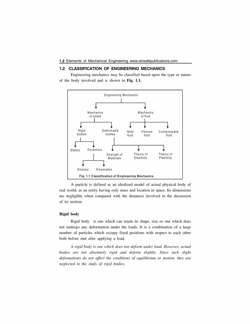
1.2 CLASSIFICATION OF ENGINEERING MECHANICSEngineering mechanics may be classified based upon the type or nature

of the body involved and is shown in Fig. 1.1.

A particle is defined as an idealized model of actual physical body of

real world, as an entity having only mass and location in space. Its dimensions

are negligible when compared with the distances involved in the discussion

of its motion.

Rigid body

Rigid body is one which can retain its shape, size or one which does

not undergo any deformation under the loads. It is a combination of a large

number of particles which occupy fixed positions with respect to each other

both before and after applying a load.

A rigid body is one which does not deform under load. However, actual

bodies are not absolutely rigid and deform slightly. Since such slight

deformations do not affect the conditions of equilibrium or motion, they are

neglected in the study of rigid bodies.

M echan icso f solids

M echan icso f fluid

R ig idbod ies

Deformablebod ies

Statics Dynam ics

Kine tics K inem atics

Strength ofM aterials

Theory o fE lasticity

Theory o fP lasticity

Idea lfluid

V iscousfluid

Compressib le fluid

Engineering M echan ics

Fig. 1.1 Classification of Engineering Mechanics

1.2 Elements of Mechanical Engineering www.airwalkpublications.com

Rigid body mechanisms found a suitable basis for the analysis anddesign of structural, mechanical or electrical engineering devices and aredivided into two areas - Statics and Dynamics. Dynamics is further dividedinto Kinetics and Kinematics.

Statics is branch of mechanics which deals with the force and itseffects on bodies at rest. The configuration of different forces is such thatthe resultant force on the system is zero.

Dynamics is branch of mechanics which deals with the force and itseffects on bodies in motion.

Kinetics is the branch of mechanics which deals with the body inmotion when the forces which cause the motion are considered.

Kinematics is the branch of mechanics which deals with the body inmotion, when the forces causing the motion are not considered.

Deformable bodies are one which undergoes deformation underapplication of forces. The branch of mechanics which deals with the studyof internal force distribution, stress and strain developed in the bodies is calledmechanics of deformable bodies or mechanics of materials.

Fluid mechanics is the branch of mechanics which deals with studyof fluids both liquids and gases at rest or in motion.

1.3 FUNDAMENTAL CONCEPTS OF MECHANICS

The basic concepts used in everyday mechanics are based on newtonianmechanics. The basic concepts used in newtonian mechanics are space, time,mass and force. These are absolute concepts because they are independentof each other.

Space is a geometric region in which events involving bodies occur.Space is associated with the position of a point P. The position of P can bedefined by three lengths measured from a certain reference point or origin inthree given directions. These lengths are known as coordinates of P.

Time is a measure of the succession of events. The standard unit used

for its measurement is the second s, which is based on duration.

Mass is used to characterize and compare bodies on the basis of certainfundamental mechanical experiments. Two bodies of the same mass, will beattracted by the earth in the same manner and, they will also offer sameresistance to a change in translation motion. Mass is quantitative measure ofinertia. Mass of a body is constant regardless of its location.


Force is the action of one body on another. Each body tends to move

in the direction of external force acting on it. A force is characterized by its

point of application, its magnitude and its direction. A force is represented

by a vector. Simply force is push or pull, which by acting on a body changes

or tends to change its state of rest or motion.

Weight is the force with which a body is attracted towards the centre

of earth by the gravitational pull. The relation between the mass and weight

of a body is given in the equation 1.1.

Weight (W) mass (m) gravity (g) ... (1.1)

where

W weight in Newton

m mass of body in kg

g acceleration due to gravity i.e 9.81 m/s2

1.4 SCALAR AND VECTOR QUANTITIESScalar quantities are those

physical quantities that have only

magnitude but no direction. eg. mass,

time, volume, etc.

Vector quantities are those

physical quantities that have both

magnitude and direction. eg.

Displacement, velocity, acceleration,

momentum, force, etc.

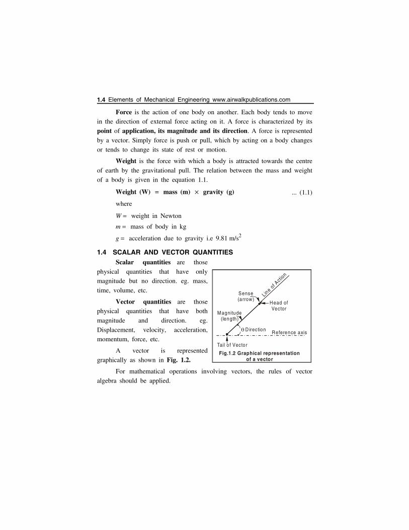
A vector is represented

graphically as shown in Fig. 1.2.

For mathematical operations involving vectors, the rules of vector

algebra should be applied.

Tail o f Vecto r

Head of Vector

Sense(arrow)

Line of Actio

n

Reference axisDirection

M agnitude (length )

Fig.1.2 Graphical representationof a vector


1.5 LAWS OF MECHANICS

The study of mechanics rests on the following fundamental principlesbased on the experimental evidences.

(i) Newton’s three fundamental laws (First law, Second law, andThird law)

(ii) Newton’s Law of Gravitation

(iii) The principle of transmissibility of forces

(iv) The parallelogram law of addition of forces

(v) The triangular law of forces

(vi) The law of conservation of Energy

(vii) The principle of work and Energy

1.5.1 Newton’s Three Fundamental Laws

(a) Newton’s First Law

Newton’s first law states that — If the net force or the resultant forceacting on a particle is zero, the particle will remain at rest (if originally atrest) or will move with constant speed in a straight line (if originally inmotion).

Or in other words, Every particle continues in its state of rest or ofmotion in a straight line unless it is compelled to change that state by anexternal force imposed on the body.

So the first law is used to define the forces.

(b) Newton’s Second LawNewton’s second law states that — If the resultant force acting on a

particle is not zero, the particle will have an acceleration proportional to themagnitude of the resultant force and will move in the direction of this resultantforce.

F Resultant force or Net force

F ma

where m Mass of the body

a Acceleration of the body

This law is used to measure a force.


Newton’s Second Law in other words:

The rate of change of momentum of a body is directly proportional tothe imposed force and it takes place in the direction in which the force acts.

i.e., Force Rate of change of momentum

Now,

Momentum Mass Velocity

Rate of change of momentum

mass rate of change of velocity

Mass Acceleration

Force mass acceleration

i.e., F ddt

mv m dvdt

m a

F K ma

K Constant of proportionality 1 in S.I. units

(c) Newton’s Third Law

Each and every action (FORCE) has equal and opposite reaction.

This means that the forces of action and reaction between two bodies

are equal in magnitude but opposite in direction and have the same line of

action.

1.5.2 Newton’s Law of Gravitation

This states that two particles of mass M and m are mutually attracted

with equal and opposite forces F and F. This force F is defined as

follows:

F G Mm

r2

where r Distance between the two particles.

G Universal constant, also called the Constant of Gravitation. Refer

Fig 1.3(a).


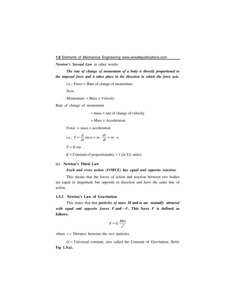
Example

The attraction of the earth on a

particle located on its surface. The force

F exerted by the earth on the particle is

known as weight W. By the law of

gravitation we have, W GMm

2,

Introducing the constant g GM

r2 , we

have

W mg

where W weight of the body in Newton N

m mass of the body in kg

g 9.81 m/sec2 acceleration due to gravity.

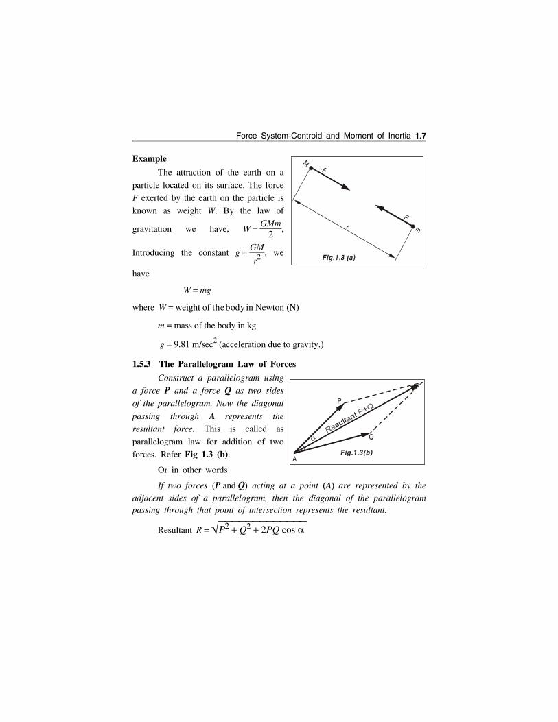
1.5.3 The Parallelogram Law of Forces

Construct a parallelogram using

a force P and a force Q as two sides

of the parallelogram. Now the diagonal

passing through A represents the

resultant force. This is called as

parallelogram law for addition of two

forces. Refer Fig 1.3 (b).

Or in other words

If two forces P and Q acting at a point A are represented by the

adjacent sides of a parallelogram, then the diagonal of the parallelogrampassing through that point of intersection represents the resultant.

Resultant R P2 Q2 2PQ cos

M

m

F

-F

r

Fig.1.3 (a)

A

Q

P

Fig.1.3(b)


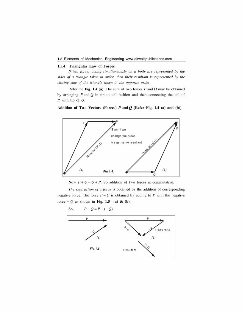
1.5.4 Triangular Law of ForcesIf two forces acting simultaneously on a body are represented by the

sides of a triangle taken in order, then their resultant is represented by the

closing side of the triangle taken in the opposite order.

Refer the Fig. 1.4 (a). The sum of two forces P and Q may be obtained

by arranging P and Q in tip to tail fashion and then connecting the tail of

P with tip of Q.

Addition of Two Vectors (Forces) P and Q [Refer Fig. 1.4 (a) and (b)]

Now P Q Q P. So addition of two forces is commutative.

The subtraction of a force is obtained by the addition of corresponding

negative force. The force P Q is obtained by adding to P with the negative

force Q as shown in Fig. 1.5 (a) & (b).

So, P Q P Q

PQ

Resultant P

+Q

P

Resulta

nt Q+P

change the order

Q

Even if we

we get sam e resultant

Fig.1.4.(a) (b)

P

Q

P- Q -Q

P

sub traction

P- QResu ltantFig.1.5.

(a) (b)


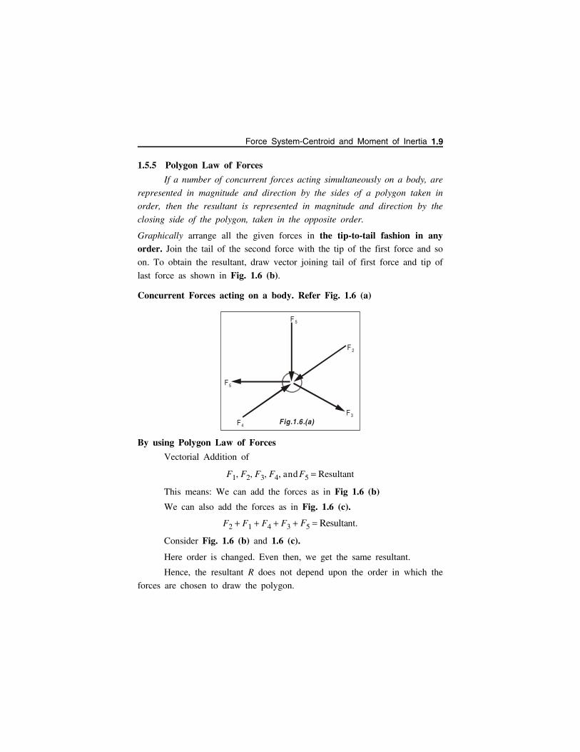
1.5.5 Polygon Law of Forces

If a number of concurrent forces acting simultaneously on a body, are

represented in magnitude and direction by the sides of a polygon taken in

order, then the resultant is represented in magnitude and direction by the

closing side of the polygon, taken in the opposite order.

Graphically arrange all the given forces in the tip-to-tail fashion in anyorder. Join the tail of the second force with the tip of the first force and so

on. To obtain the resultant, draw vector joining tail of first force and tip of

last force as shown in Fig. 1.6 (b).

Concurrent Forces acting on a body. Refer Fig. 1.6 (a)

By using Polygon Law of Forces

Vectorial Addition of

F1, F2, F3, F4, and F5 Resultant

This means: We can add the forces as in Fig 1.6 (b)

We can also add the forces as in Fig. 1.6 (c).

F2 F1 F4 F3 F5 Resultant.

Consider Fig. 1.6 (b) and 1.6 (c).

Here order is changed. Even then, we get the same resultant.

Hence, the resultant R does not depend upon the order in which the

forces are chosen to draw the polygon.

F5

Fig.1.6.(a)

F 5

F 2

F3

F4


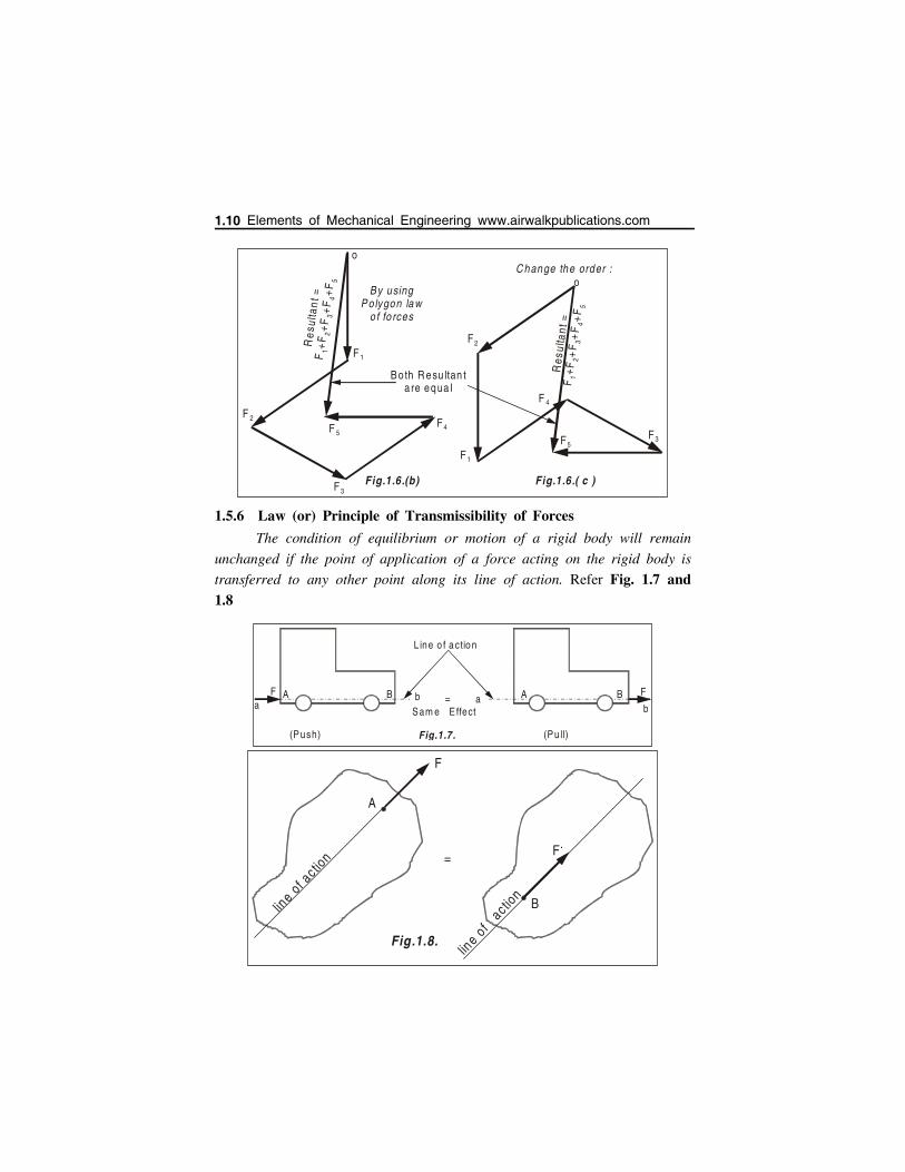
1.5.6 Law (or) Principle of Transmissibility of Forces

The condition of equilibrium or motion of a rigid body will remain

unchanged if the point of application of a force acting on the rigid body is

transferred to any other point along its line of action. Refer Fig. 1.7 and1.8

F 1

F 2

F3

F4F 5

By using Po lygon law

o f fo rces

o

F1

F2

F3

F 4

F5

Res

ult a

n t =

F

+ F+

F+

F+

F1

23

45

oC hange the order :

Res

ulta

nt =

F

+F

+ F+ F

+ F1

23

45

Bo th R esu ltan t a re equa l

Fig.1.6.(b) Fig.1.6.( c )

aF A B b a A B

b=

L ine o f a ctio n

F

Sam e E ffect

(Push) (Pu ll)Fig.1.7 .

A

line o

f ac tio

n

F

= F �

line o

f a

c tion

B

Fig.1.8.


A force F acting on a body at point A is transferred to point B along

the same line of action without changing its net effect on the rigid body.

Principle of Transmissibility in other words (Refer Fig. 1.8)

Alternatively, the principle of transmissibility states that the conditions

of equilibrium or the motion of a rigid body will remain unchanged if a force

F acting at a given point ‘A’ of the rigid body is replaced by a force F of

the same magnitude and same direction, but acting at a different point ‘B’,provided that the two forces have the same line of action. The two forces

F and F have the same effect on the rigid body and are said to be equivalent.

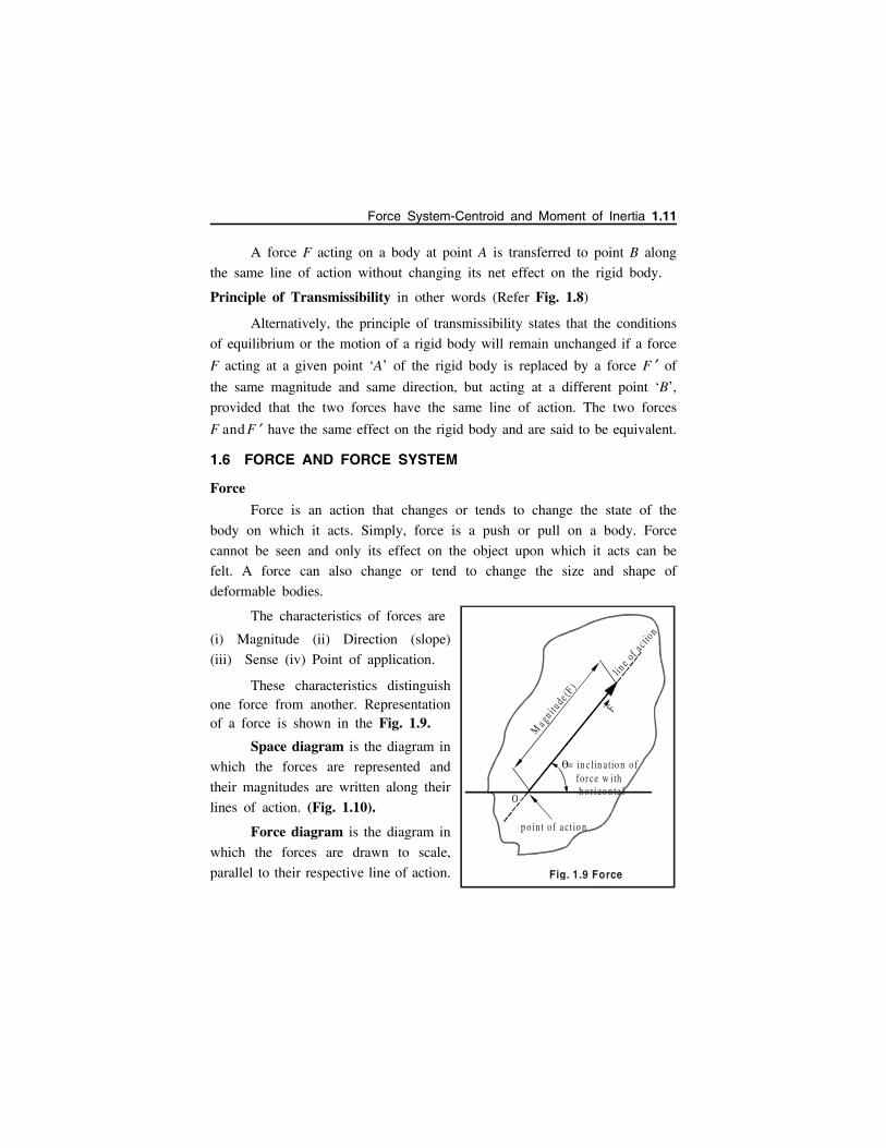
1.6 FORCE AND FORCE SYSTEM

Force

Force is an action that changes or tends to change the state of the

body on which it acts. Simply, force is a push or pull on a body. Force

cannot be seen and only its effect on the object upon which it acts can be

felt. A force can also change or tend to change the size and shape of

deformable bodies.

The characteristics of forces are

(i) Magnitude (ii) Direction (slope)

(iii) Sense (iv) Point of application.

These characteristics distinguishone force from another. Representationof a force is shown in the Fig. 1.9.

Space diagram is the diagram in

which the forces are represented and

their magnitudes are written along their

lines of action. (Fig. 1.10).

Force diagram is the diagram in

which the forces are drawn to scale,

parallel to their respective line of action.

O

p oin t o f a c t io n

= in c lin a tio n o f for ce w ith h o rizo n ta l

F

Magn

itude (F

)

l ine o

f ac tio

n

Fig. 1.9 Force


1.6.1 Types of forces

Forces may be classified as

(i) External forces (contacting or applied forces)

(ii) Body forces (non-contacting or non applied forces)

(a) External forces

Forces which act on a body due to external causes or agency are termed

as external forces. The external forces acting on the surface of a body are

called surface forces. The equilibrium of the body is affected by all the

external forces (body forces and contact forces) which act on the body.

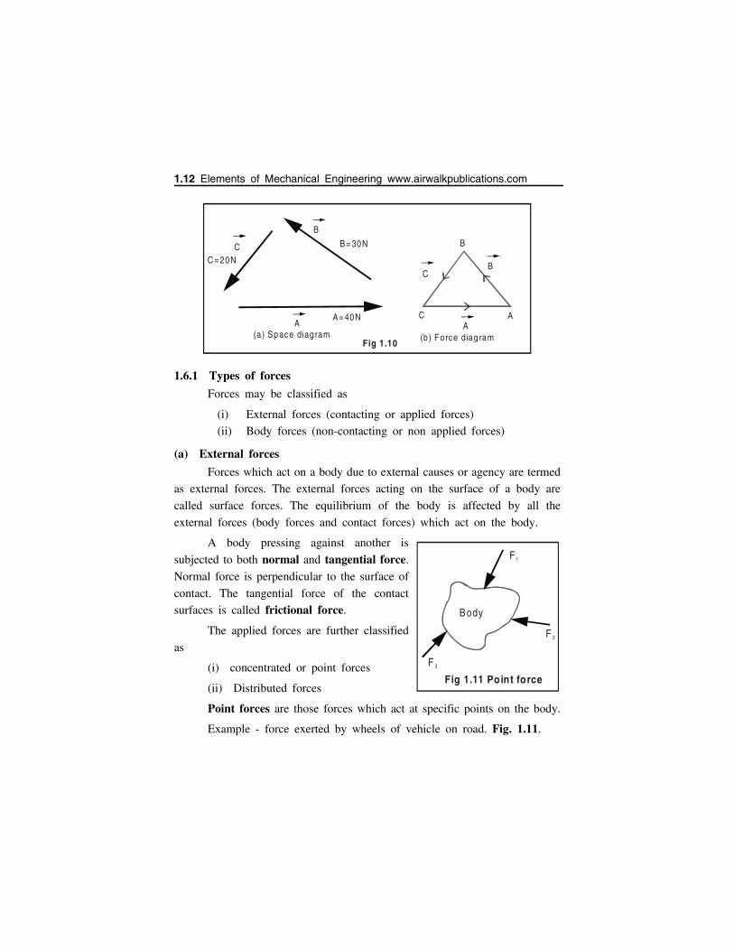
A body pressing against another is

subjected to both normal and tangential force.

Normal force is perpendicular to the surface of

contact. The tangential force of the contact

surfaces is called frictional force.

The applied forces are further classified

as

(i) concentrated or point forces

(ii) Distributed forces

Point forces are those forces which act at specific points on the body.

Example - force exerted by wheels of vehicle on road. Fig. 1.11.

C

B

AA= 40N

C =20N

B= 30N

(a ) Sp ace diag ram

B

CB

AAC

(b) Fo rce diag ramFig 1.10

Body

F 3

F 2

F1

Fig 1.11 Point force


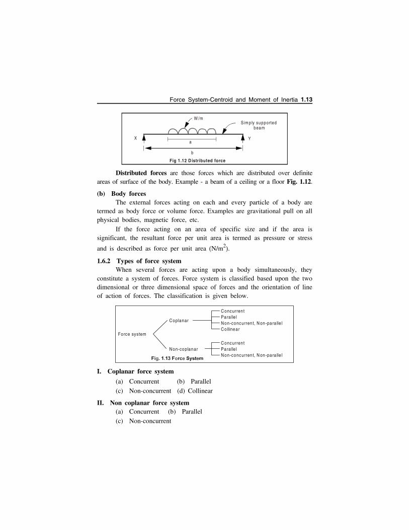
Distributed forces are those forces which are distributed over definiteareas of surface of the body. Example - a beam of a ceiling or a floor Fig. 1.12.

(b) Body forcesThe external forces acting on each and every particle of a body are

termed as body force or volume force. Examples are gravitational pull on allphysical bodies, magnetic force, etc.

If the force acting on an area of specific size and if the area issignificant, the resultant force per unit area is termed as pressure or stress

and is described as force per unit area N/m2.

1.6.2 Types of force systemWhen several forces are acting upon a body simultaneously, they

constitute a system of forces. Force system is classified based upon the twodimensional or three dimensional space of forces and the orientation of lineof action of forces. The classification is given below.

I. Coplanar force system

(a) Concurrent (b) Parallel

(c) Non-concurrent (d) Collinear

II. Non coplanar force system(a) Concurrent (b) Parallel

(c) Non-concurrent

W /mSim p ly supported

bea m

YXa

b

Fig 1.12 D istributed force

Force system

Coplanar

Non-coplanar

Concurren tParalle lNon-concurren t, N on-para lle lCo llinear

Concurren tParalle lNon-concurren t, N on-para lle l


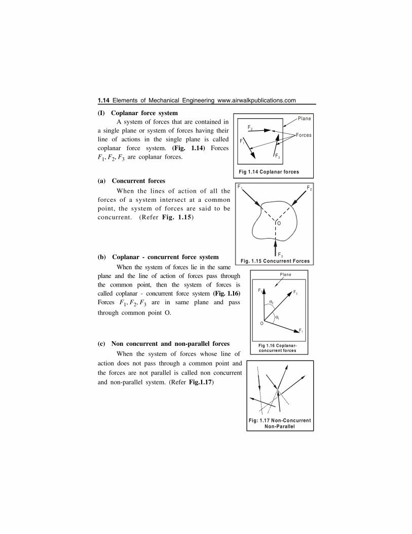
(I) Coplanar force systemA system of forces that are contained in

a single plane or system of forces having theirline of actions in the single plane is calledcoplanar force system. (Fig. 1.14) ForcesF1, F2, F3 are coplanar forces.

(a) Concurrent forces

When the lines of action of all theforces of a system intersect at a commonpoint, the system of forces are said to beconcurrent. (Refer Fig. 1.15)

(b) Coplanar - concurrent force system

When the system of forces lie in the sameplane and the line of action of forces pass throughthe common point, then the system of forces iscalled coplanar - concurrent force system (Fig. 1.16)Forces F1, F2, F3 are in same plane and pass

through common point O.

(c) Non concurrent and non-parallel forces

When the system of forces whose line of

action does not pass through a common point and

the forces are not parallel is called non concurrent

and non-parallel system. (Refer Fig.1.17)

Fig 1.14 Coplanar forces

F1

F 2

F3

Forces

Plane

O1

2

F 3 F2

F1

Fig 1.16 Coplanar- concurrent fo rces

Plane

O

F 1 F 2

F3

Fig. 1.15 Concurrent Forces

Fig: 1.17 Non-ConcurrentNon-Parallel


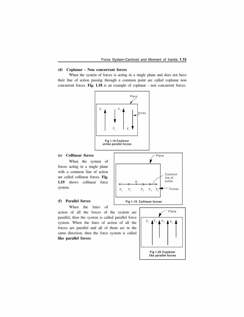
(d) Coplanar - Non concurrent forcesWhen the system of forces is acting in a single plane and does not have

their line of action passing through a common point are called coplanar nonconcurrent forces. Fig. 1.18 is an example of coplanar - non concurrent forces.

(e) Collinear forces

When the system offorces acting in a single planewith a common line of actionare called collinear forces. Fig.1.19 shows collinear forcesystem.

(f) Parallel forces

When the lines ofaction of all the forces of the system areparallel, then the system is called parallel forcesystem. When the lines of action of all theforces are parallel and all of them act in thesame direction, then the force system is calledlike parallel forces.

O

F 2 F1 F3 F 4 F5

Comm online ofaction

Forces

Fig 1.19 Collinear forces

Plane

F 1F 2 F3 F 4

P lane

Fig 1.20 Coplanarlike parallel forces

F 1

F 2

F 3

P lane

fo rces

Fig 1.18 Coplanar un like parallel forces


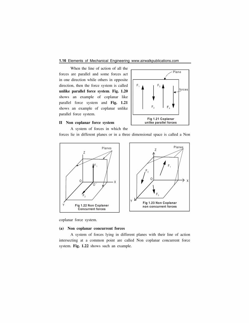
When the line of action of all the

forces are parallel and some forces act

in one direction while others in opposite

direction, then the force system is called

unlike parallel force system. Fig. 1.20shows an example of coplanar like

parallel force system and Fig. 1.21shows an example of coplanar unlike

parallel force system.

II Non coplanar force system

A system of forces in which the

forces lie in different planes or in a three dimensional space is called a Non

coplanar force system.

(a) Non coplanar concurrent forces

A system of forces lying in different planes with their line of action

intersecting at a common point are called Non coplanar concurrent force

system. Fig. 1.22 shows such an example.

F 1

F2

F3

P lane

forces

Fig 1.21 Coplanar unlike parallel forces

X

Y

Z

O

F1

F2

Planes

Fig 1.23 Non Coplanar non concurrent forces

F3

X

Y

Z

O

F 1

O ’

F2

Fig 1.22 Non Coplaner Concurrent forces

Plan es


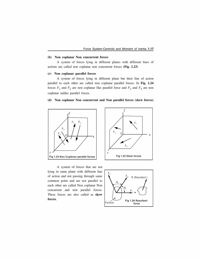
(b) Non coplanar Non concurrent forces

A system of forces lying in different planes with different lines of

actions are called non coplanar non concurrent forces (Fig. 1.23)

(c) Non coplanar parallel forces

A system of forces lying in different plane but their line of action

parallel to each other are called non coplanar parallel forces. In Fig. 1.24forces F1 and F2 are non coplanar like parallel force and F3 and F4 are non

coplanar unlike parallel forces.

(d) Non coplanar Non concurrent and Non parallel forces (skew forces)

A system of forces that are not

lying in same plane with different line

of action and not passing through same

common point and are not parallel to

each other are called Non coplanar Non

concurrent and non parallel forces.

These forces are also called as skewforces.

X

Y

Z

O

F1 F 2

F3

F 4

Fig 1.24 Non Coplanar parallel forces

X

Y

Z

O

F 1

F 2

F3

Fig 1.25 Skew forces

F3F2

F1

R (Resultan t )

Fig 1.26 Resultant forceParticle


1.7 COMPOSITION OF FORCESComposition of a force system is a process of finding a single force,

known as resultant, that can produce the same effect on the particle as that

of the system of forces. For example Fig. 1.26 shows a system of three forces

acting on a particle with the resultant R which can produce the same effect.

A particle means that the size and shape of body does not significantly

affect the solution of problems and all the forces are assumed to act at the

same point.

Thus, the resultant is a representative force which has the sameeffect on the particle as the group of forces it replaces.

1.7.1 Resultant of two coplanar concurrent forces

Resultant of two coplanar concurrent forces can be obtained by the

following methods.

1. Analytical method

(a) Parallelogram law of forces

(b) Triangular law of forces

2. Graphical method

(a) Parallelogram law of forces, (b) Triangular law of forces

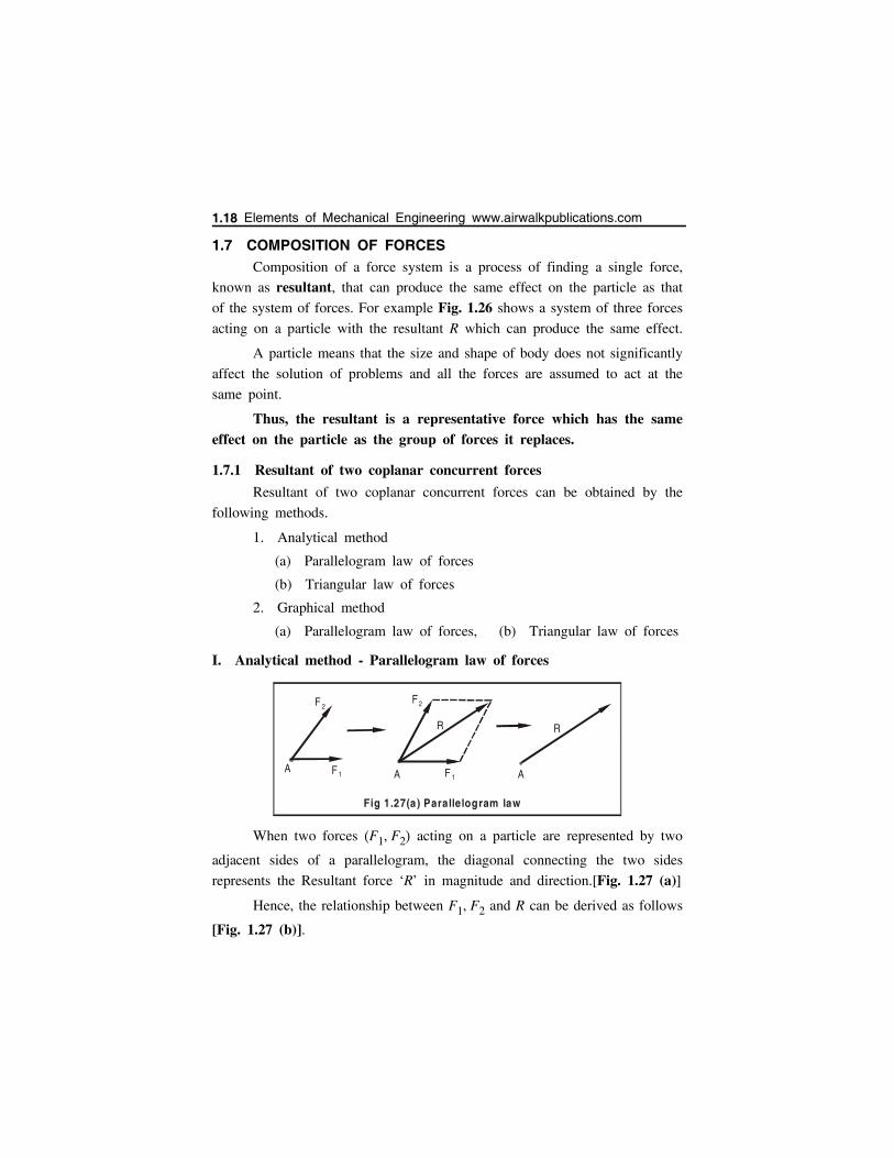
I. Analytical method - Parallelogram law of forces

When two forces F1, F2 acting on a particle are represented by two

adjacent sides of a parallelogram, the diagonal connecting the two sides

represents the Resultant force ‘R’ in magnitude and direction.[Fig. 1.27 (a)]

Hence, the relationship between F1, F2 and R can be derived as follows

[Fig. 1.27 (b)].

F 2

A F1

R

F2

F 1

R

Fig 1.27(a) Parallelogram law

AA


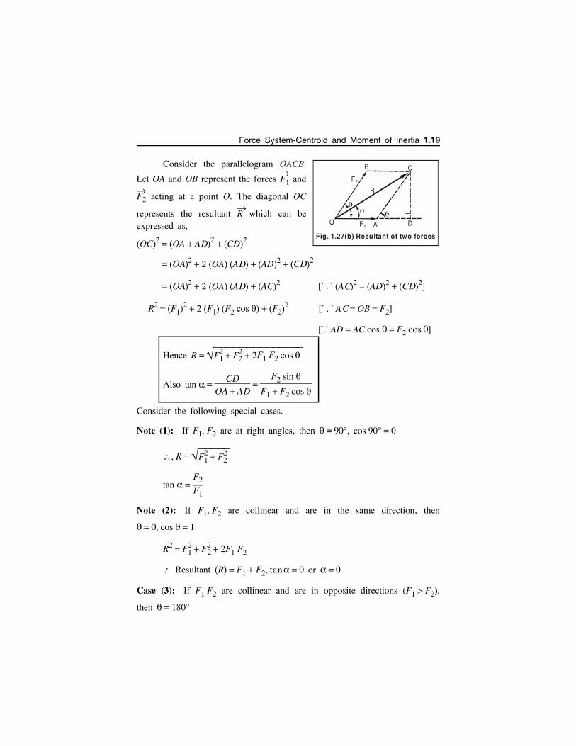
Consider the parallelogram OACB.

Let OA and OB represent the forces F

1 and

F

2 acting at a point O. The diagonal OC

represents the resultant R

which can beexpressed as,

OC2 OA AD2 CD2

OA2 2 OA AD AD2 CD2

OA2 2 OA AD AC2 [. . . AC2 AD2 CD2]

R2 F12 2 F1 F2 cos F2

2 [. . . AC OB F2]

[... AD AC cos F2 cos ]

Hence R F12 F2

2 2F1 F2 cos

Also tan CD

OA AD

F2 sin F1 F2 cos

Consider the following special cases.

Note (1): If F1, F2 are at right angles, then 90, cos 90 0

, R F12 F2

2

tan F2F1

Note (2): If F1, F2 are collinear and are in the same direction, then

0, cos 1

R2 F12 F2

2 2F1 F2

Resultant R F1 F2, tan 0 or 0

Case (3): If F1 F2 are collinear and are in opposite directions F1 F2,

then 180

O F1 A D

R

B C

F2

Fig. 1.27(b) Resultant of two forces


R2 F12 F2

2 2F1 F2, R F1 F2

tan 0: 0

Problem 1.1: The maximum and minimum resultant of two forces acting ona particle are 50 kN and 10 kN respectively. If 50 kN is the magnitude ofthe resultant for the given system of forces F1 and F2, find the angle between

F1 & F2.

Solution:

We know that Resultant of two coplanar concurrent forces is

R2 F12 F2

2 2F1 R2 cos

When R is maximum 0 i.e., 50 F1 F2

When R is minimum, 180 i.e., 10 F1 F2

Solving the above two equations, we get F1 30 kN and F2 20 kN

If the resultant of forces F1, F2 acting at an angle ‘’ is 50 kN,

502 302 202 2 30 20 cos

cos 1 or 0

Thus F1 and F2 are collinear to each other when the resultant is 50kN.

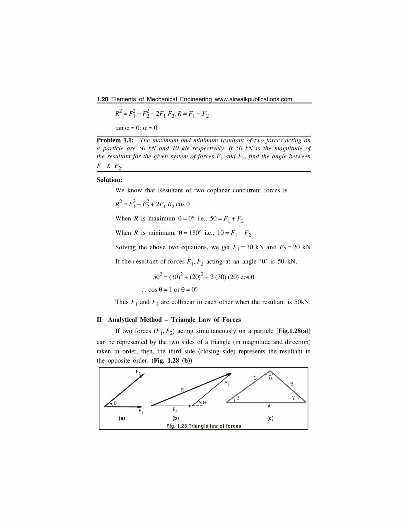
II Analytical Method – Triangle Law of Forces

If two forces F1, F2 acting simultaneously on a particle [Fig.1.28(a)]

can be represented by the two sides of a triangle (in magnitude and direction)

taken in order, then, the third side (closing side) represents the resultant in

the opposite order. (Fig. 1.28 (b))

F1

F2

F1

RF2

Fig. 1.28 Triangle law of forces

A

BC

(a) (b) (c)


Thus trigonometric relations can be applied. From Fig. 1.28(c), we have

Asin

B

sin

Csin

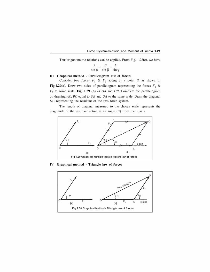
III Graphical method - Parallelogram law of forcesConsider two forces F1 & F2 acting at a point O as shown in

Fig.1.29(a). Draw two sides of parallelogram representing the forces F1 &

F2 to some scale. Fig. 1.29 (b) as OA and OB. Complete the parallelogram

by drawing AC, BC equal to OB and OA to the same scale. Draw the diagonalOC representing the resultant of the two force system.

The length of diagonal measured to the chosen scale represents the

magnitude of the resultant acting at an angle from the x axis.

IV Graphical method - Triangle law of forces

F2

F1

O

(a)

O

B C

A

F 2

F1

R

(b )

x ax is

Fig 1.29 Graphical method- parallelogram law of forces

B

A

Resu ltant(R )

O

F2

F1

x axis(a)O

F2

F 1(b)


Consider two forces F1 and F2 as shown in Fig. 1.30 (a). Draw OA

to some scale as shown in the Fig. 1.30 (b). From the end A, draw AB to

same scale. Join OB as the closing side of triangle. The length OB to the

same scale represents the magnitude of the resultant of the two forces F1 &

F2. The angle represents the angle of resultant taken from x axis.

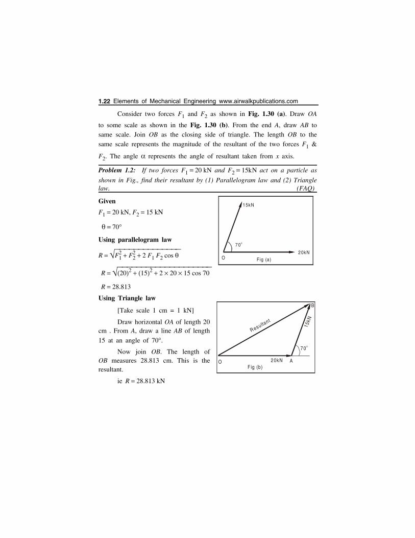
Problem 1.2: If two forces F1 20 kN and F2 15kN act on a particle as

shown in Fig., find their resultant by (1) Parallelogram law and (2) Trianglelaw. (FAQ)

Given

F1 20 kN, F2 15 kN

70

Using parallelogram law

R F12 F2

2 2 F1 F2 cos

R 202 152 2 20 15 cos 70

R 28.813

Using Triangle law

[Take scale 1 cm = 1 kN]

Draw horizontal OA of length 20cm . From A, draw a line AB of length

15 at an angle of 70.

Now join OB. The length ofOB measures 28.813 cm. This is theresultant.

ie R 28.813 kN

70o

15kN

20kN

R esultant

F ig (b)O A

B


70o

15kN

20kNO Fig (a)

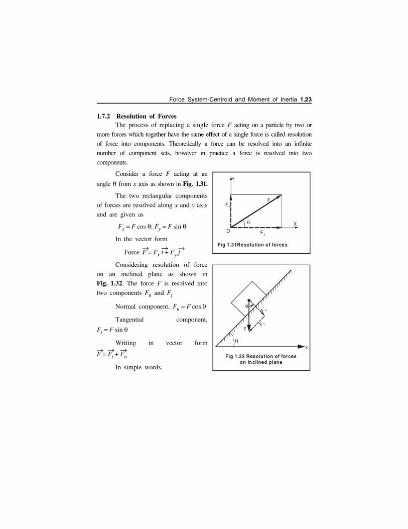
1.7.2 Resolution of ForcesThe process of replacing a single force F acting on a particle by two or

more forces which together have the same effect of a single force is called resolution

of force into components. Theoretically a force can be resolved into an infinite

number of component sets, however in practice a force is resolved into two

components.

Consider a force F acting at an

angle from x axis as shown in Fig. 1.31.

The two rectangular components

of forces are resolved along x and y axis

and are given as

Fx F cos ; Fy F sin

In the vector form

Force F

Fx i Fy j

Considering resolution of force

on an inclined plane as shown in

Fig. 1.32. The force F is resolved into

two components Fn and Ft

Normal component, Fn F cos

Tangential component,

Ft F sin

Writing in vector form

F

Ft

Fn

In simple words,

Fig 1.31Resolution o f fo rces

Y

X

Fy

F x

F

O

F

x

Fig 1 .32 Resolution of forces on inclined plane

F t

F n


Resolution (projection) of Forces into components

A single force can be resolvedinto two components which give thesame effect on the particle. ReferFig.1.33.

Now a force F is resolved as -Horizontal component of ‘F’ i.e.

“F cos ” and Vertical component of

‘F’ i.e. “F sin ”.

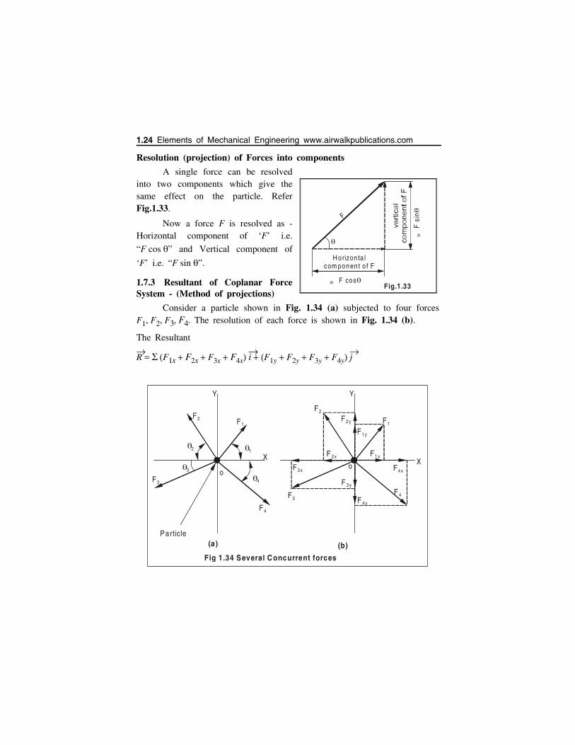
1.7.3 Resultant of Coplanar ForceSystem - (Method of projections)

Consider a particle shown in Fig. 1.34 (a) subjected to four forcesF1, F2, F3, F4. The resolution of each force is shown in Fig. 1.34 (b).

The Resultant

R

F1x F2x F3x F4x i F1y F2y F3y F4y j

H orizon ta lcom ponen t o f F

F s

in

=

F cos=

F

Fig.1.33

Fig 1.34 Several C oncurrent forces

X

Y

F1

F2

F3

F 4

Particle(a)

o

2 1

3

4

(b)

X

Y

F1

F2

F3F 4

o

F2 y

F 2 x

F1 y

F1 x

F4 x

F 4 y

F 3 y

F3 x


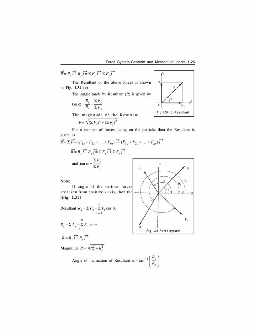
R

Rx i Ry j

Fx i

Fy j

The Resultant of the above forces is shownin Fig. 1.34 (c).

The Angle made by Resultant R is given by

tan Ry

Rx Fy

Fx

The magnitude of the Resultant

F Fx2 Fy

2

For n number of forces acting on the particle, then the Resultant isgiven as

R

F

F1x F2x Fnx i F1y F2y Fny j

R

Rx i Ry j

Fx i

Fy j

and tan Fy

Fx

Note:If angle of the various forces

are taken from positive x axis, then the(Fig. 1.35)

Resultant Rx Fx i 1

n

Fi cos i

Ry Fy i 1

n

Fi sin i

R Rx i Ry j

Magnitude R Rx2 Ry

2

Angle of inclination of Resultant tan 1 RyRx

R y

R

X

R xO

Y

Fig 1.34 (c) Resultant

X

YF 1F 2

F 4

F3Fig 1 .35 Force system

1

2

3

4


1.7.4 Summary

Resultant Force

Two or more forces on a particle may

be replaced by a single force called resultant

force which gives a same effect.

The resultant force, of a given system of

forces, is found out by the method of resolution

as followed:

1. Resolve all the forces vertically and add

all the vertical components (i.e., Find

Fy)

2. Resolve all the forces horizontally and add all the horizontal components

(i.e., Find Fx)

3. The resultant R of the given forces is given by the equation:

R Fy2 Fx

2

4. The resultant force will be inclined at an angle , with the horizontal.

tan

Fy

Fx

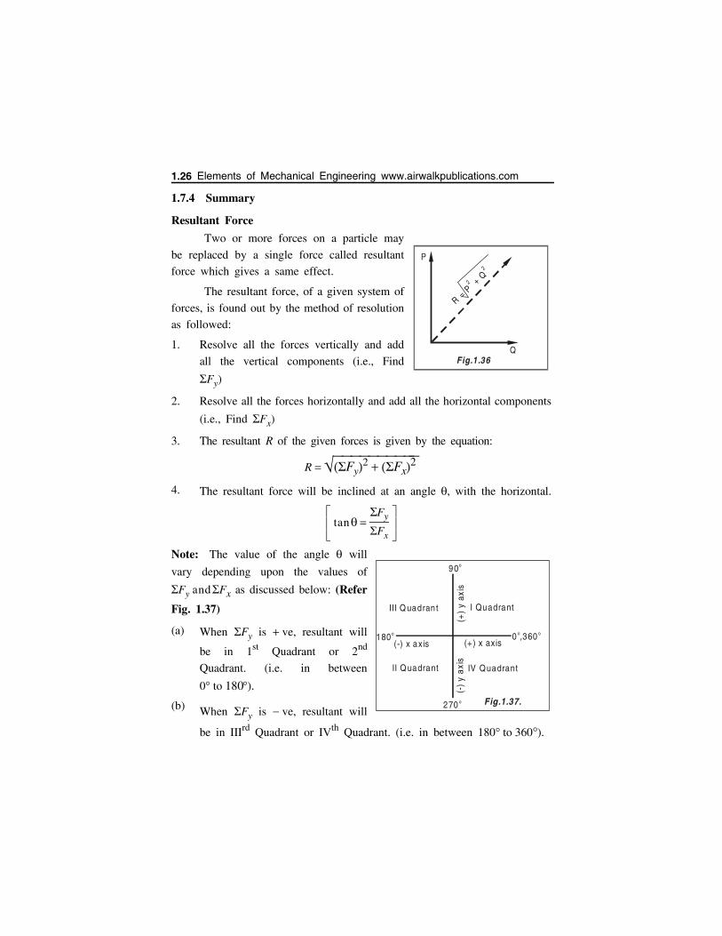
Note: The value of the angle will

vary depending upon the values of

Fy and Fx as discussed below: (Refer

Fig. 1.37)

(a) When Fy is ve, resultant will

be in 1st Quadrant or 2nd

Quadrant. (i.e. in between

0 to 180).

(b) When Fy is ve, resultant will

be in IIIrd Quadrant or IVth Quadrant. (i.e. in between 180 to 360).

P

Q

R = P +

Q2

2

Fig.1.36

I Quadrant

II Q uadrant

III Q uadran t

IV Quadrant

0 ,360o o

270 o

180o

90o

(-) x ax is

(-)

y ax

is(+

) y

axis

(+ ) x axis

Fig.1.37.


(c) When Fx is ve, the resultant will be in Ist Quadrant or IVth Quadrant

(i.e. in between 0 to 90 or 270 to 360).

(d) When Fx is ve, the resultant will be in IInd Quadrant or IIIrd

Quadrant. (i.e. in between 90 to 180 or 180 to 270).

The following sign conventions are followed for solving staticsproblems.

Sign conventions for the direction of force:

‘x’ axis Right side ‘’ ve.

‘x’ axis Left side ‘’ ve

‘y’ axis Upside ‘’ ve

‘y’ axis Downward ‘’ ve

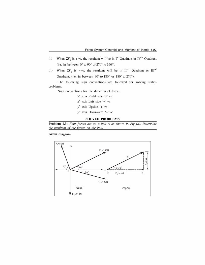
SOLVED PROBLEMSProblem 1.3: Four forces act on a bolt A as shown in Fig (a). Determinethe resultant of the forces on the bolt.

Given diagram

F cos 1

Fsi

n1

F 1

F =150N1

F =110N3

F =100N4

F =80N2

o x

y

Fig.(a)

30o70o

15o

Fig.(b)

=30 o


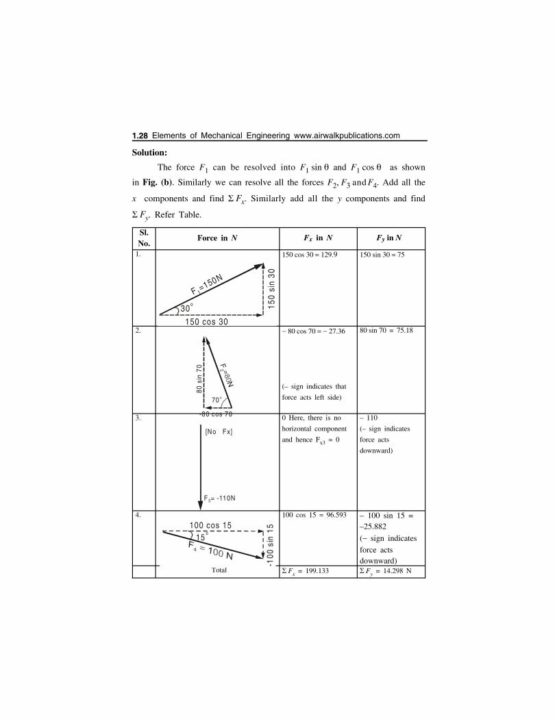
Solution:

The force F1 can be resolved into F1 sin and F1 cos as shown

in Fig. (b). Similarly we can resolve all the forces F2, F3 and F4. Add all the

x components and find Fx. Similarly add all the y components and find

Fy. Refer Table.

Sl.No.

Force in N Fx in N Fy in N

1. 150 cos 30 129.9 150 sin 30 75

2. 80 cos 70 27.36

(– sign indicates that

force acts left side)

80 sin 70 = 75.18

3. 0 Here, there is no

horizontal component

and hence Fx3 = 0

– 110

(– sign indicates

force acts

downward)

4. 100 cos 15 = 96.593 – 100 sin 15 =–25.882

( sign indicates

force actsdownward)

Total Fx = 199.133 Fy = 14.298 N

30o

F =150N1

150 cos 30

150

sin

30

70 o

-80 cos 70

80 s

in 7

0

[No Fx]

F = -110N3

15o

-100

sin

15100 cos 15


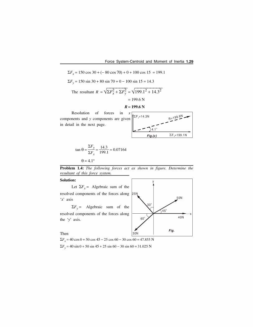
Fx 150 cos 30 80 cos 70 0 100 cos 15 199.1

Fy 150 sin 30 80 sin 70 0 100 sin 15 14.3

The resultant R Fx2 Fy

2 199.12 14.32

199.6 N

R 199.6 NResolution of forces in x

components and y components are given

in detail in the next page.

tan Fy

Fx

14.3199.1

0.07164

4.1

Problem 1.4: The following forces act as shown in figure. Determine theresultant of this force system.

Solution:

Let Fx Algebraic sum of the

resolved components of the forces along

‘x’ axis

Fy Algebraic sum of the

resolved components of the forces along

the ‘y’ axis.

Then

Fx 40 cos 0 50 cos 45 25 cos 60 30 cos 60 47.855 N

Fy 40 sin 0 50 sin 45 25 sin 60 30 sin 60 31.025 N

45o

30o

60 o

30N

25N50N

40Nx

y

Fig.

R=199.6NF =14.3Ny

F =199.1NxFig.(c)

4.1 o


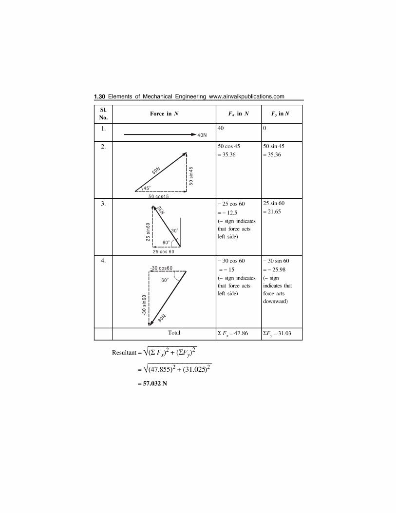
Sl.No.

Force in N Fx in N Fy in N

1. 40 0

2. 50 cos 45

35.36

50 sin 45

35.36

3. 25 cos 60

12.5

(– sign indicatesthat force actsleft side)

25 sin 60

21.65

4. 30 cos 60

15

(– sign indicatesthat force actsleft side)

30 sin 60

25.98

(– signindicates thatforce actsdownward)

Total Fx 47.86 Fy 31.03

Resultant Fx2 Fy

2

47.8552 31.0252

57.032 N

40N

50N

45o

50

sin

455 0 cos45

25 s

in60

2 5 cos 60

25N

60 o

30o

-30

sin6

0

-30 cos60

30N

60o


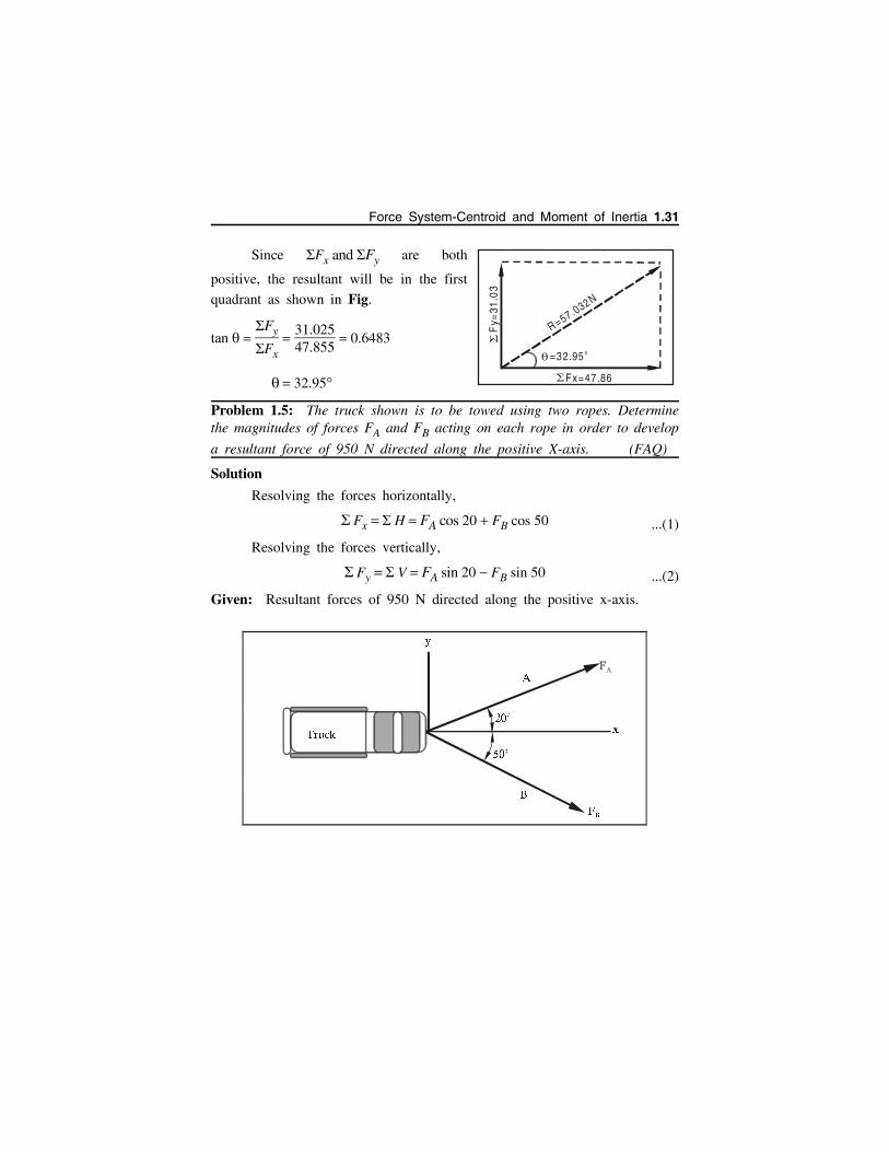
Since Fx and Fy are both

positive, the resultant will be in the first

quadrant as shown in Fig.

tan Fy

Fx

31.02547.855

0.6483

32.95

Problem 1.5: The truck shown is to be towed using two ropes. Determinethe magnitudes of forces FA and FB acting on each rope in order to develop

a resultant force of 950 N directed along the positive X-axis. (FAQ)

Solution

Resolving the forces horizontally,

Fx H FA cos 20 FB cos 50 ...(1)

Resolving the forces vertically,

Fy V FA sin 20 FB sin 50 ...(2)

Given: Resultant forces of 950 N directed along the positive x-axis.

R=57 .032N

=32.95 o

Fx=47 .86

Fy=

31.0

3

��

�

�

��

��

�

�

��


So H 950 N and V 0 apply on equation (1) & (2)

(1) 950 FA cos 20 FB cos 50 ...(3)

(2) 0 FA sin 20 FB sin 50

FA sin 20 FB sin 50

FA FB sin 50

sin 20

FA 2.2397 FB ...(4)

Subtitute equation (4), in equation (3)

(3) 950 [2.2397 FB cos 20] FB cos 50

950 2.104 FB 0.642 FB

950 2.746 FB

FB 345.86 N

(4) FA 2.2397 345.86

FA 774.62 N

Result

FA 774.62 N, FB 345.86 N

Problem 1.6: Determine the resultant of the concurrent force system shownin Figure (a).

Fx H

150 cos 30 200 cos 30 80 cos 60 180 cos 45

43.98 N

Fy V

150 sin 30 200 sin 30 80 sin 60 180 sin 45

21.56 N


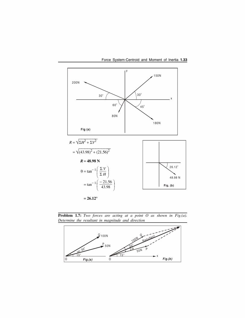
R H2 V2

43.982 21.562

R 48.98 N

tan 1 V

H

tan 1 21.5643.98

26.12

Problem 1.7: Two forces are acting at a point O as shown in Fig.(a).Determine the resultant in magnitude and direction

180N

80N

150N

200N

30o

60o

30o

45o

Fig (a)

y

x

26.12 o

48.98 N

Fig. (b)

100N

50N

Q

P

= 30o

15o

O

100N

50N

Q

P3 0

o

15 o

O

Resultant

Fig.(b)Fig.(a)

x


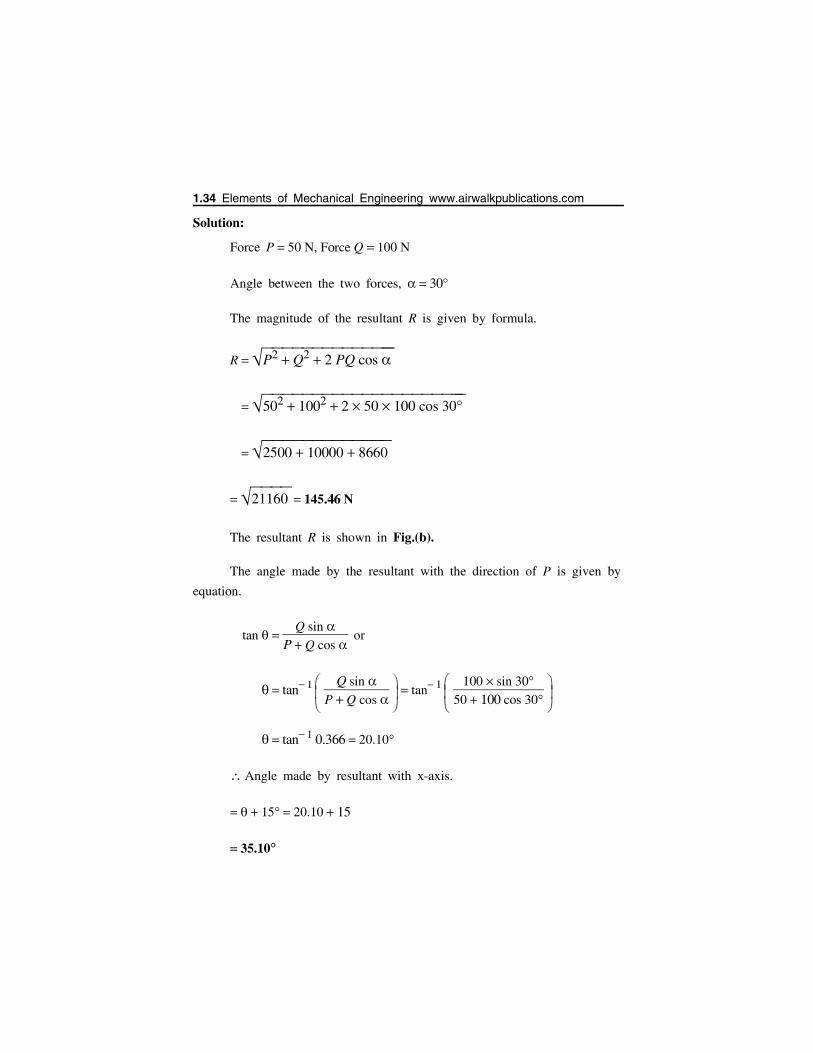
Solution:

Force P 50 N, Force Q 100 N

Angle between the two forces, 30

The magnitude of the resultant R is given by formula.

R P2 Q2 2 PQ cos

502 1002 2 50 100 cos 30

2500 10000 8660

21160 145.46 N

The resultant R is shown in Fig.(b).

The angle made by the resultant with the direction of P is given by

equation.

tan Q sin

P Q cos or

tan 1

Q sin P Q cos

tan 1

100 sin 3050 100 cos 30

tan 1 0.366 20.10

Angle made by resultant with x-axis.

15 20.10 15

35.10


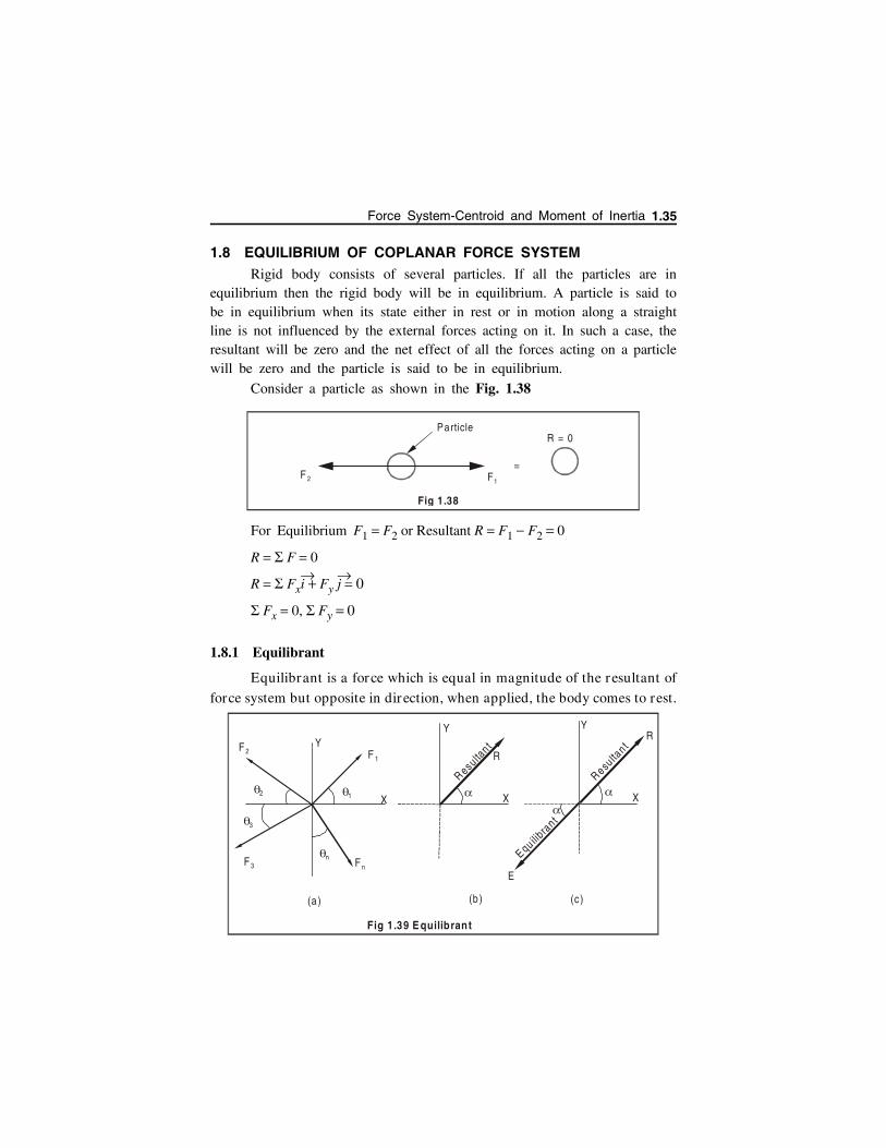
1.8 EQUILIBRIUM OF COPLANAR FORCE SYSTEMRigid body consists of several particles. If all the particles are in

equilibrium then the rigid body will be in equilibrium. A particle is said tobe in equilibrium when its state either in rest or in motion along a straightline is not influenced by the external forces acting on it. In such a case, theresultant will be zero and the net effect of all the forces acting on a particlewill be zero and the particle is said to be in equilibrium.

Consider a particle as shown in the Fig. 1.38

For Equilibrium F1 F2 or Resultant R F1 F2 0

R F 0

R Fxi Fy j

0

Fx 0, Fy 0

1.8.1 Equilibrant

Equilibrant is a force which is equal in magnitude of the resultant of

force system but opposite in direction, when applied, the body comes to rest.

Particle

F 2 F1

Fig 1.38

=

R = 0

X

YF 1

F 2

F3 Fn

2 1

3

n

(a ) (b )

Fig 1.39 E quilibrant

E

RY

X

(c)

Y

X

Resultan t

R

Resulta

nt

Equ ilibra

nt


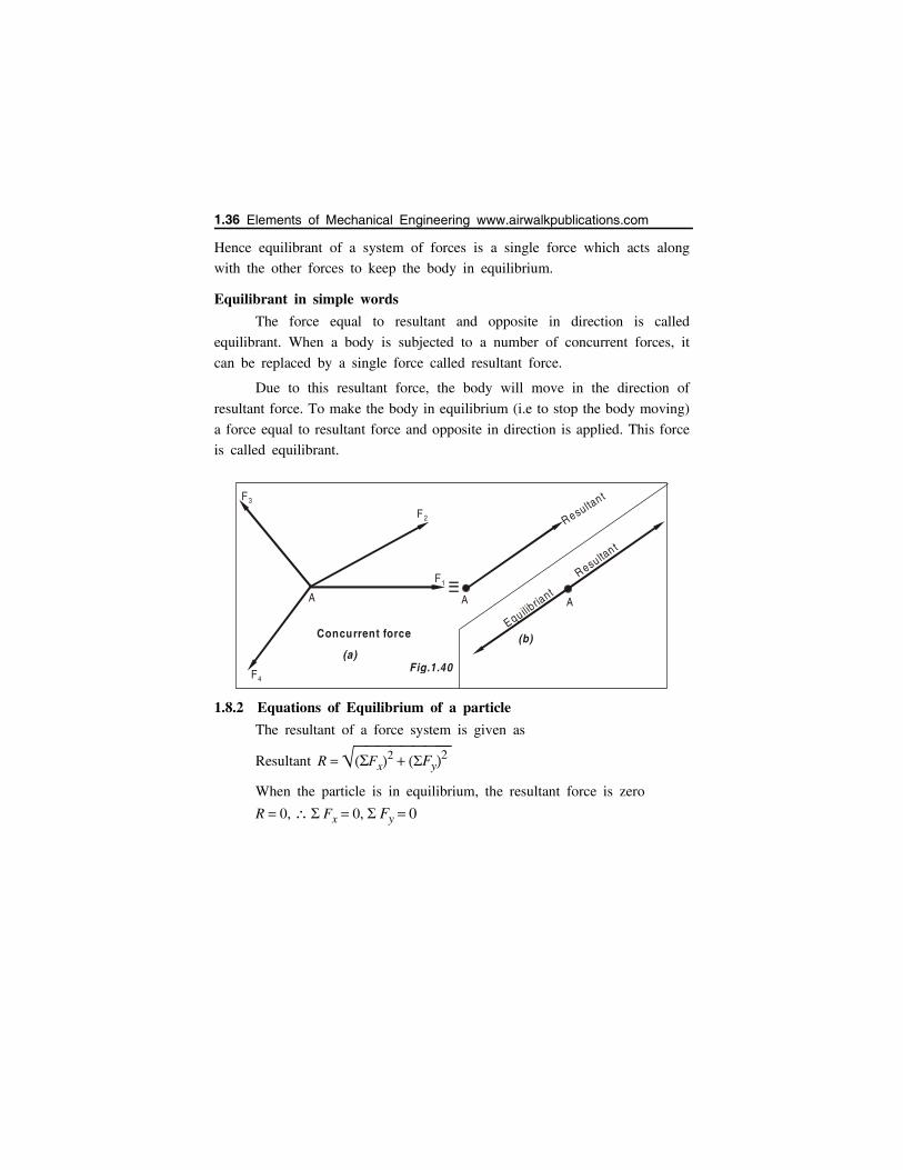
Hence equilibrant of a system of forces is a single force which acts along

with the other forces to keep the body in equilibrium.

Equilibrant in simple words

The force equal to resultant and opposite in direction is called

equilibrant. When a body is subjected to a number of concurrent forces, it

can be replaced by a single force called resultant force.

Due to this resultant force, the body will move in the direction of

resultant force. To make the body in equilibrium (i.e to stop the body moving)

a force equal to resultant force and opposite in direction is applied. This force

is called equilibrant.

1.8.2 Equations of Equilibrium of a particle

The resultant of a force system is given as

Resultant R Fx2 Fy

2

When the particle is in equilibrium, the resultant force is zero

R 0, Fx 0, Fy 0

A

F1

F 2

F3

F4

A A

Equilibria

nt

Resulta

n t

Resultan t

Concurrent force

Fig.1.40(a)

(b)


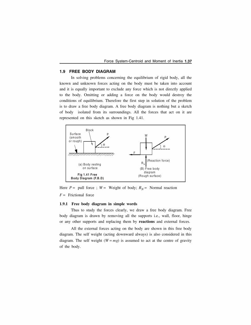
1.9 FREE BODY DIAGRAMIn solving problems concerning the equilibrium of rigid body, all the

known and unknown forces acting on the body must be taken into account

and it is equally important to exclude any force which is not directly applied

to the body. Omitting or adding a force on the body would destroy the

conditions of equilibrium. Therefore the first step in solution of the problem

is to draw a free body diagram. A free body diagram is nothing but a sketch

of body isolated from its surroundings. All the forces that act on it are

represented on this sketch as shown in Fig 1.41.

Here P pull force ; W Weight of body; RN Normal reaction

F Frictional force

1.9.1 Free body diagram in simple words

Thus to study the forces clearly, we draw a free body diagram. Free

body diagram is drawn by removing all the supports i.e., wall, floor, hinge

or any other supports and replacing them by reactions and external forces.

All the external forces acting on the body are shown in this free body

diagram. The self weight (acting downward always) is also considered in this

diagram. The self weight (W mg) is assumed to act at the centre of gravity

of the body.

BlockPSurface

(sm oo th o r rough)

(a ) Body resting on su rface

Fig 1 .41 Free Body Diagram (F.B.D)

F

(B) Free bo dy d iagram

(Ro ugh su rfa ce )

R N

PW

(Re action fo rce)


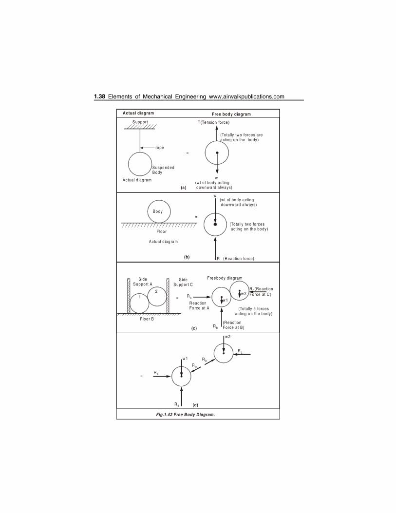
rope

Suspe nded Body

Actual d iagram

Suppor t

Actual d iagram

Body

Floor

R (Reaction fo rce)

(Totally two fo rces acting on the bo dy)

(w t of body ac ting downw ard alw ays)

(w t of body ac ting downw ard alw ays)

T(Tension fo rce)

(Totally two fo rces a reacting on the bo dy)

w

w

SideSuppor t A

SideSuppor t C

12

Floor B

R A

R B

R eactionForce at A

(ReactionForce at B)

Fre ebody d iagram

w 1

w 2

(Totally 5 fo rces acting on the body)

Actual diagram Free body diagram

R (ReactionForce at C )

C

Fig.1.42 Free Body Diagram.

R A

R B

w 1

w 2

R C

R D

R D

=

=

=

=

(a)

(b)

(c)

(d)


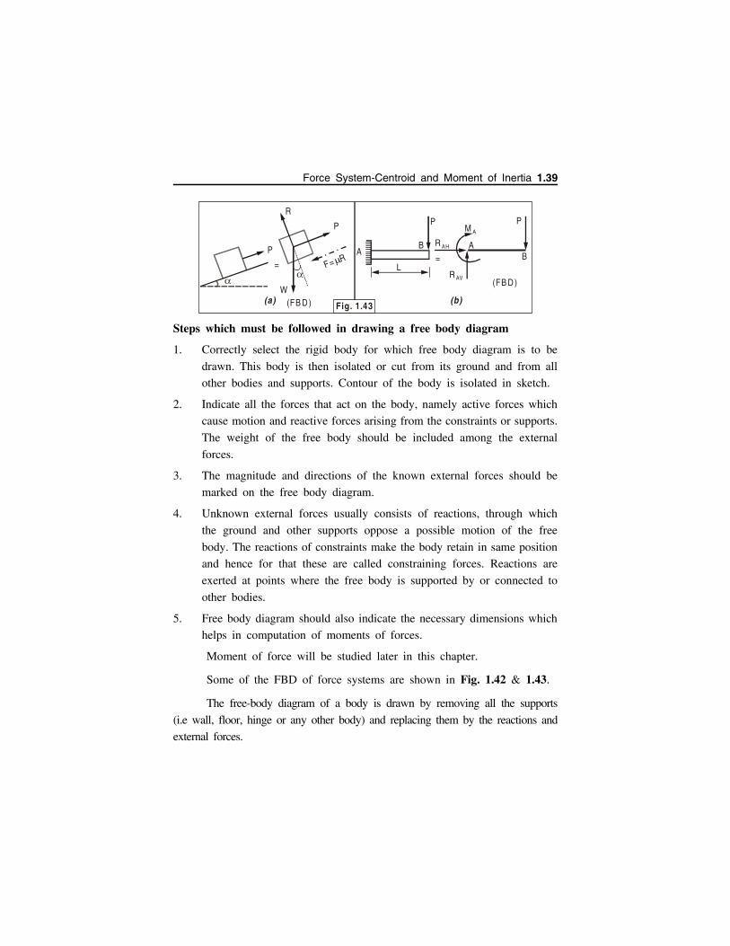
Steps which must be followed in drawing a free body diagram

1. Correctly select the rigid body for which free body diagram is to be

drawn. This body is then isolated or cut from its ground and from all

other bodies and supports. Contour of the body is isolated in sketch.

2. Indicate all the forces that act on the body, namely active forces which

cause motion and reactive forces arising from the constraints or supports.

The weight of the free body should be included among the external

forces.

3. The magnitude and directions of the known external forces should be

marked on the free body diagram.

4. Unknown external forces usually consists of reactions, through which

the ground and other supports oppose a possible motion of the free

body. The reactions of constraints make the body retain in same position

and hence for that these are called constraining forces. Reactions are

exerted at points where the free body is supported by or connected to

other bodies.

5. Free body diagram should also indicate the necessary dimensions which

helps in computation of moments of forces.

Moment of force will be studied later in this chapter.

Some of the FBD of force systems are shown in Fig. 1.42 & 1.43.

The free-body diagram of a body is drawn by removing all the supports

(i.e wall, floor, hinge or any other body) and replacing them by the reactions and

external forces.

P

R

P

W

F= RA

B

L

R AH

M A

R AV

A

P

B

(FB D )

(FB D )(a) (b)

P

==

Fig. 1.43


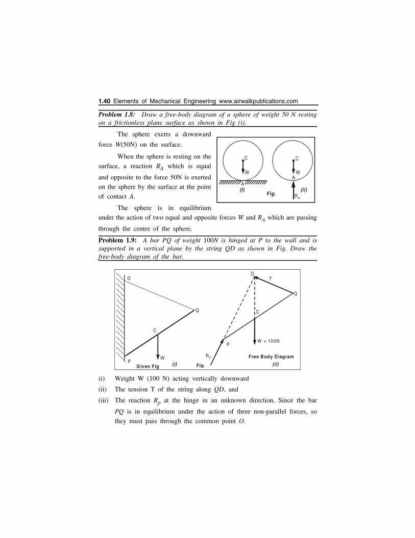
Problem 1.8: Draw a free-body diagram of a sphere of weight 50 N restingon a frictionless plane surface as shown in Fig (i).

The sphere exerts a downward

force W50N on the surface.

When the sphere is resting on the

surface, a reaction RA which is equal

and opposite to the force 50N is exerted

on the sphere by the surface at the point

of contact A.

The sphere is in equilibrium

under the action of two equal and opposite forces W and RA which are passing

through the centre of the sphere.

Problem 1.9: A bar PQ of weight 100N is hinged at P to the wall and issupported in a vertical plane by the string QD as shown in Fig. Draw thefree-body diagram of the bar.

(i) Weight W (100 N) acting vertically downward

(ii) The tension T of the string along QD, and

(iii) The reaction Rp at the hinge in an unknown direction. Since the bar

PQ is in equilibrium under the action of three non-parallel forces, so

they must pass through the common point O.

A

R AFig.

A

W

C

W

C

(I) (ii)

P

P

Q

Q

D

W

W = 100N

C

C

OT

R P

Fig.(i) (ii)G iven Fig

Free B ody Diagram


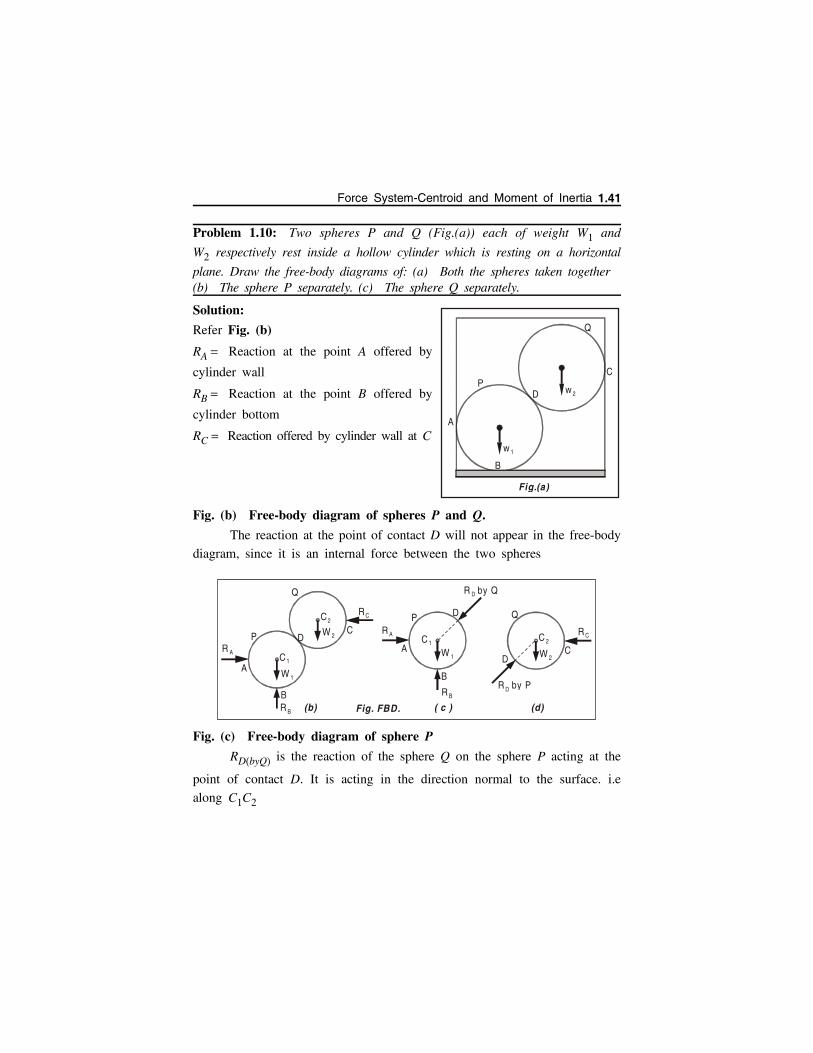
Problem 1.10: Two spheres P and Q (Fig.(a)) each of weight W1 and

W2 respectively rest inside a hollow cylinder which is resting on a horizontal

plane. Draw the free-body diagrams of: (a) Both the spheres taken together (b) The sphere P separately. (c) The sphere Q separately.

Solution:

Refer Fig. (b)

RA Reaction at the point A offered by

cylinder wall

RB Reaction at the point B offered by

cylinder bottom

RC Reaction offered by cylinder wall at C

Fig. (b) Free-body diagram of spheres P and Q.

The reaction at the point of contact D will not appear in the free-body

diagram, since it is an internal force between the two spheres

Fig. (c) Free-body diagram of sphere P

RDbyQ is the reaction of the sphere Q on the sphere P acting at the

point of contact D. It is acting in the direction normal to the surface. i.e

along C1C2

A

P

Q

C

B

D

Fig.(a)

w 1

w 2

R A

R A

R B

R B

R C

R C

A

AP

P

Q

Q

D

D

D

W 2

W 2

C 2

C 2

C

CC 1

C 1

W 1

W 1

B

BR by PD

(b) Fig. FBD. ( c ) (d)

R by QD


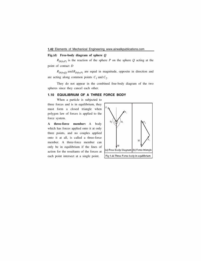
Fig.(d) Free-body diagram of sphere Q

RDbyP is the reaction of the sphere P on the sphere Q acting at the

point of contact D

RDbyQ and RDbyP are equal in magnitude, opposite in direction and

are acting along common points C1 and C2.

They do not appear in the combined free-body diagram of the two

spheres since they cancel each other.

1.10 EQUILIBRIUM OF A THREE FORCE BODYWhen a particle is subjected to

three forces and is in equilibrium, they

must form a closed triangle when

polygon law of forces is applied to the

force system.

A three-force member: A body

which has forces applied onto it at only

three points, and no couples applied

onto it at all, is called a three-force

member. A three-force member can

only be in equilibrium if the lines of

action for the resultants of the forces at

each point intersect at a single point.

F 2

F 1

12

W

W F 1

F 2


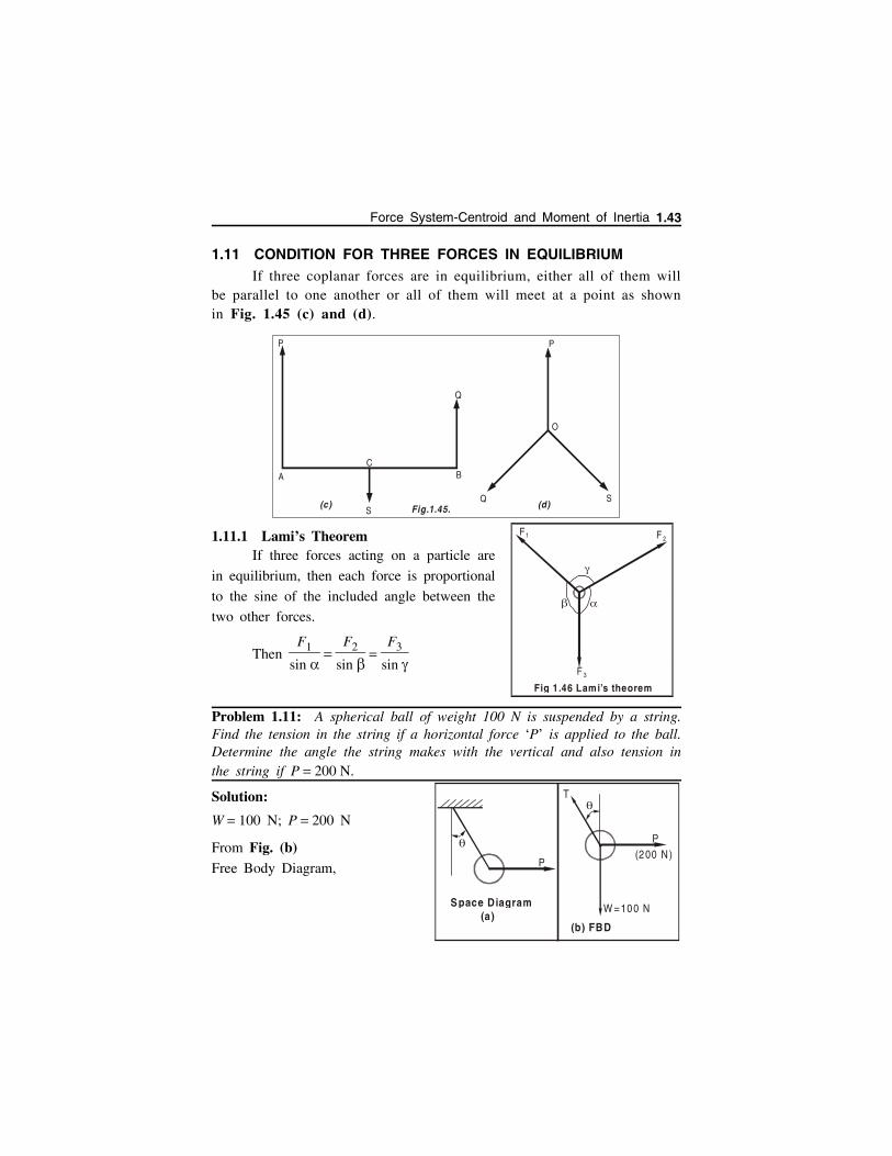
1.11 CONDITION FOR THREE FORCES IN EQUILIBRIUMIf three coplanar forces are in equilibrium, either all of them will

be parallel to one another or all of them will meet at a point as shownin Fig. 1.45 (c) and (d).

1.11.1 Lami’s TheoremIf three forces acting on a particle are

in equilibrium, then each force is proportional

to the sine of the included angle between the

two other forces.

Then F1

sin

F2

sin

F3

sin

Problem 1.11: A spherical ball of weight 100 N is suspended by a string.Find the tension in the string if a horizontal force ‘P’ is applied to the ball.Determine the angle the string makes with the vertical and also tension inthe string if P 200 N.

Solution:

W 100 N; P 200 N

From Fig. (b) Free Body Diagram,

A BC

S

P

Q

P

Q S

O

Fig.1.45.(c) (d)

F1 F 2

F 3

Fig 1.46 Lami’s theorem

P

(a)

P

T

(b) FBD

W =100 N

(200 N)

Space Diagram


Using Equations of equilibrium,

Fx 0; T sin 200 0

Fy 0; T cos 100 0

T sin 200

T cos 100

tan 2

tan 1 2 63.43

T sin 63.43 200

T 200

sin 63.43 223.6 N

Using Lami’s Theorem (Fig. (c))

Tsin 90

W

sin 90

Psin 180

Tsin 90

100

sin 90

200sin 180

Tsin 90 100 sin 90 100

T cos 100 ...(i)

T sin 180 200 sin 90 200

T sin 200 ...(ii)

Dividing (ii) by (i)

T sin T cos

200100

2; tan 2

tan 1 2 63.43

T sin 200

T sin 63.43 200

T 223.6 N


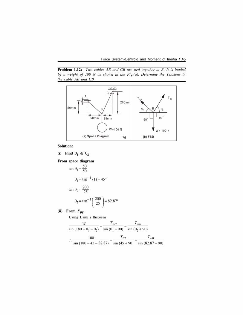
Problem 1.12: Two cables AB and CB are tied together at B. It is loadedby a weight of 100 N as shown in the Fig.(a). Determine the Tensions inthe cable AB and CB

Solution:

(i) Find 1 & 2

From space diagram

tan 1 5050

1 tan 1 1 45

tan 2 20025

2 tan 1 20025

82.87

(ii) From FBD

Using Lami’s theroem

Wsin 180 1 2

TBC

sin 1 90

TAB

sin 2 90

100

sin 180 45 82.87

TBC

sin 45 90

TAB

sin 82.87 90

50m m

50m m 25m m

B

200 mm

CA

W =100 N

(a) Space Diagram Fig (b) FBD

B1 2

90o

90o

W = 100 N

T ABT BC


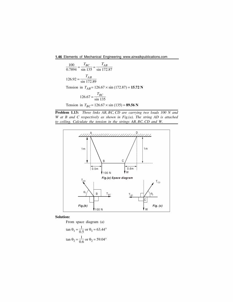
1000.7894

TBC

sin 135

TAB

sin 172.87

126.92 TAB

sin 172.89

Tension in TAB 126.67 sin 172.87 15.72 N

126.67 TBC

sin 135

Tension in TBC 126.67 sin 135 89.56 N

Problem 1.13: Three links AB, BC, CD are carrying two loads 100 N andW at B and C respectively as shown in Fig.(a). The string AD is attachedto ceiling. Calculate the tension in the strings AB, BC, CD and W.

Solution:From space diagram (a)

tan 1 1

0.5 or 1 63.44

tan 2 1

0.6 or 2 59.04

0.5m

B

1m

A

C

D

0.6m

1m

100 N W

Fig.(a) Space diagram

T B C

TC D

W

21 B

C

T B C

100 N

TA B

Fig.(b) Fig. (c)


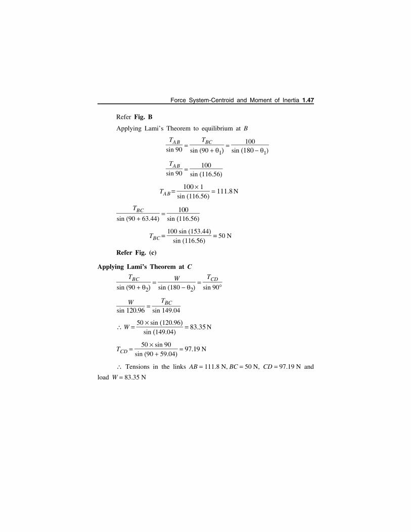
Refer Fig. B

Applying Lami’s Theorem to equilibrium at B

TAB

sin 90

TBC

sin 90 1

100sin 180 1

TAB

sin 90

100sin 116.56

TAB 100 1

sin 116.56 111.8 N

TBC

sin 90 63.44

100sin 116.56

TBC 100 sin 153.44

sin 116.56 50 N

Refer Fig. (c)

Applying Lami’s Theorem at C

TBC

sin 90 2

Wsin 180 2

TCD

sin 90

Wsin 120.96

TBC

sin 149.04

W 50 sin 120.96

sin 149.04 83.35 N

TCD 50 sin 90

sin 90 59.04 97.19 N

Tensions in the links AB 111.8 N, BC 50 N, CD 97.19 N and

load W 83.35 N


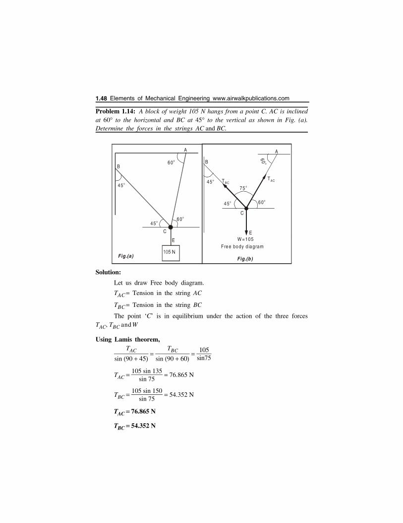
Problem 1.14: A block of weight 105 N hangs from a point C. AC is inclinedat 60 to the horizontal and BC at 45 to the vertical as shown in Fig. (a).Determine the forces in the strings AC and BC.

Solution:

Let us draw Free body diagram.

TAC Tension in the string AC

TBC Tension in the string BC

The point ‘C’ is in equilibrium under the action of the three forcesTAC, TBC and W

Using Lamis theorem,TAC

sin 90 45

TBC

sin 90 60

105sin75

TAC 105 sin 135

sin 75 76.865 N

TBC 105 sin 150

sin 75 54.352 N

TAC 76.865 N

TBC 54.352 N

A

B

C

45o

60o

60o

45 o

E

Fig.(a)

B

A

C

45 o

45o

75 o

60o

60o

EW =105

TACTBC

Fre e body d iagram

Fig.(b)


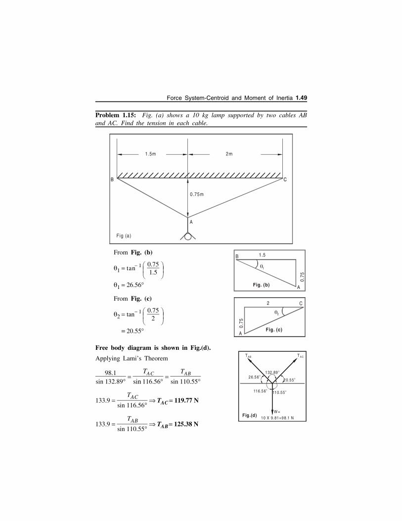
Problem 1.15: Fig. (a) shows a 10 kg lamp supported by two cables ABand AC. Find the tension in each cable.

From Fig. (b)

1 tan 1 0.751.5

1 26.56

From Fig. (c)

2 tan 1 0.75

2

20.55

Free body diagram is shown in Fig.(d).

Applying Lami’s Theorem

98.1sin 132.89

TAC

sin 116.56

TAB

sin 110.55

133.9 TAC

sin 116.56 TAC 119.77 N

133.9 TAB

sin 110.55 TAB 125.38 N

1 .5m 2m

0.75m

A

B C

Fig (a)

1

1 .5B

A

0.75

Fig. (b)

A

C

2

2

0.75

Fig. (c)

116.56o

110.55o

26.56 o

20.55o

132 .89 o

T A B T A C

10 X 9.81=98.1 N

W =Fig.(d)


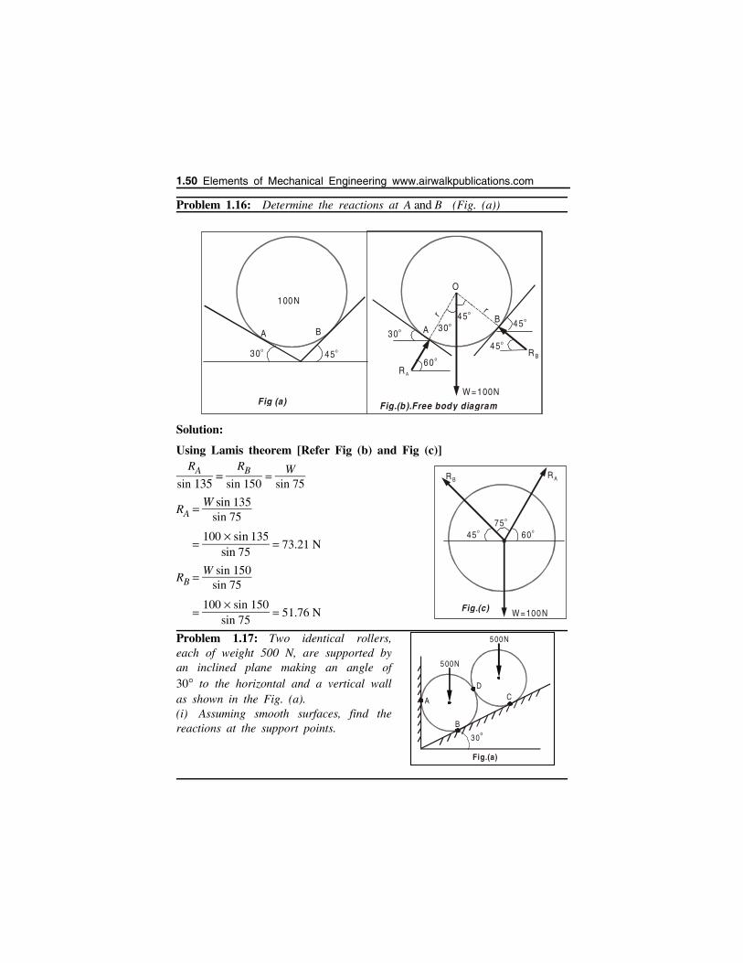
Problem 1.16: Determine the reactions at A and B (Fig. (a))

Solution:

Using Lamis theorem [Refer Fig (b) and Fig (c)]RA

sin 135

RB

sin 150

Wsin 75

RA W sin 135

sin 75

100 sin 135

sin 75 73.21 N

RB W sin 150

sin 75

100 sin 150

sin 75 51.76 N

Problem 1.17: Two identical rollers,each of weight 500 N, are supported byan inclined plane making an angle of30 to the horizontal and a vertical wallas shown in the Fig. (a).(i) Assuming smooth surfaces, find thereactions at the support points.

45o30o

A B

100N

Fig (a)

30o45o

30o45o

45o

O

ABr

r

60o

R A

R B

W =100N

Fig.(b).Free body diagram

60o45o

W =100N

R AR B

Fig.(c)

75o

30o

500N

500N

A

B

CD

Fig.(a)


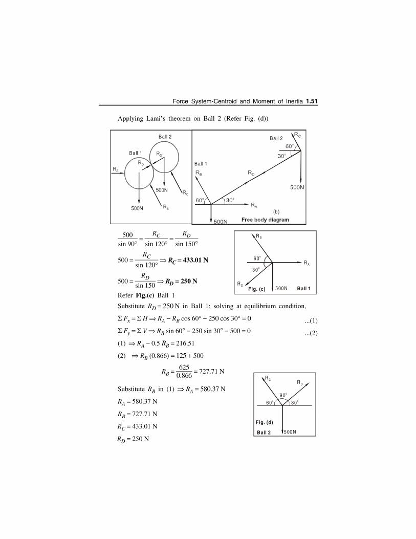
Applying Lami’s theorem on Ball 2 (Refer Fig. (d))

500sin 90

RC

sin 120

RD

sin 150

500 RC

sin 120 RC 433.01 N

500 RD

sin 150 RD 250 N

Refer Fig.(c) Ball 1

Substitute RD 250 N in Ball 1; solving at equilibrium condition,

Fx H RA RB cos 60 250 cos 30 0 ...(1)

Fy V RB sin 60 250 sin 30 500 0 ...(2)

(1) RA 0.5 RB 216.51

(2) RB 0.866 125 500

RB 625

0.866 727.71 N

Substitute RB in (1) RA 580.37 N

RA 580.37 N

RB 727.71 N

RC 433.01 N

RD 250 N

(b )

Ba ll 1

Ba ll 1

Ba ll 2 Ba ll 2

Fig. (d)

60o

R C R D

30o

500N

90o

Ball 2

60o

R A

R B

R D

30o

500NFig. (c) Ball 1


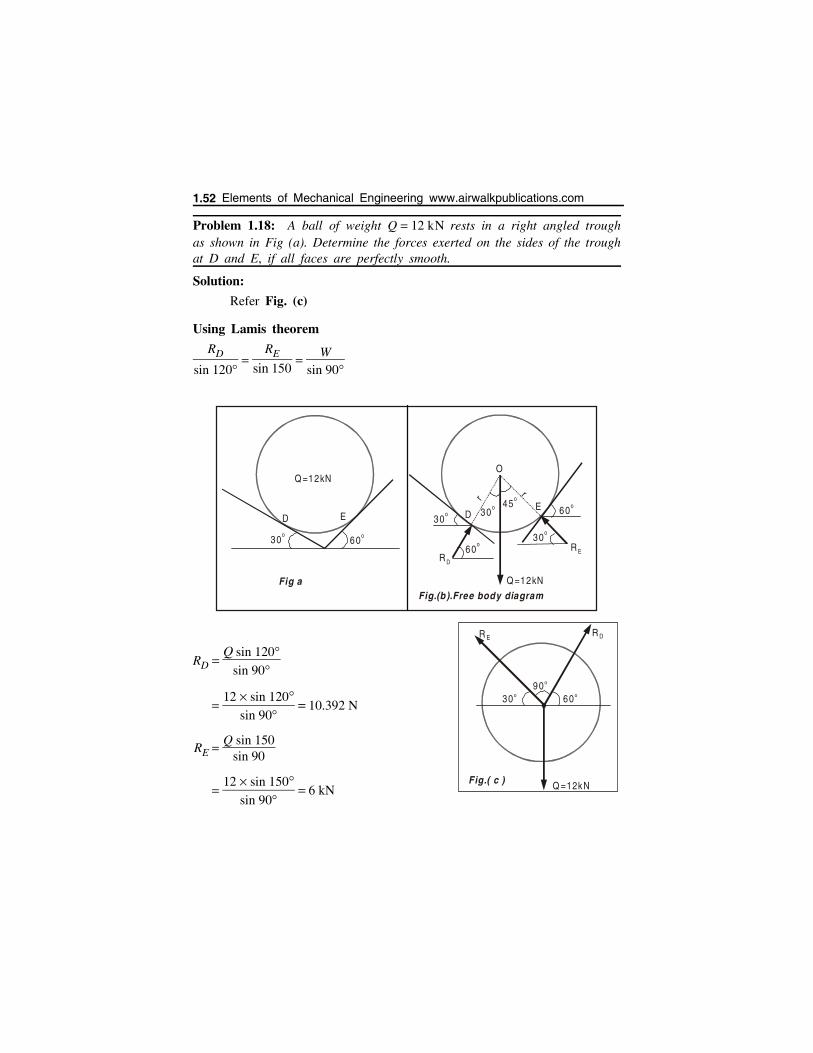
Problem 1.18: A ball of weight Q 12 kN rests in a right angled troughas shown in Fig (a). Determine the forces exerted on the sides of the troughat D and E, if all faces are perfectly smooth.

Solution:

Refer Fig. (c)

Using Lamis theorem

RD

sin 120

RE

sin 150

Wsin 90

RD Q sin 120

sin 90

12 sin 120

sin 90 10.392 N

RE Q sin 150

sin 90

12 sin 150

sin 90 6 kN

60o30

o

D E

Q =12kN

Fig a

30o 45

o

30o 60

o

30o

O

DE

r r

60o

R D

R E

Q =12kN

Fig.(b).Free body diagram

60o30o

Q =12kN

R DR E

Fig.( c )

90o


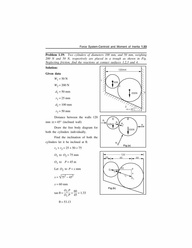
Problem 1.19: Two cylinders of diameters 100 mm, and 50 mm, weighing200 N and 50 N, respectively are placed in a trough as shown in Fig.Neglecting friction, find the reactions at contact surfaces 1,2,3 and 4.

Solution:

Given data

W1 50 N

W2 200 N

d1 50 mm

r1 25 mm

d2 100 mm

r2 50 mm

Distance between the walls 120

mm 45 (inclined wall)

Draw the free body diagram for

both the cylinders individually.

Find the inclination of both the

cylinders let it be inclined at .

r1 r2 25 50 75

O1 to O2 75 mm

O1 to P 45 m

Let O2 to P x mm

x 752 452

x 60 mm

tan O2 P

O1 P

6045

1.33

53.13

50N

200N

120mm

1

3

4

2= 45o

2R 1

R 2

R 4R 450N

200 N

1

Fig.(a)

R 3

12025 5045

45O 1

O 2

r2

r1

P

x

Fig.(b)


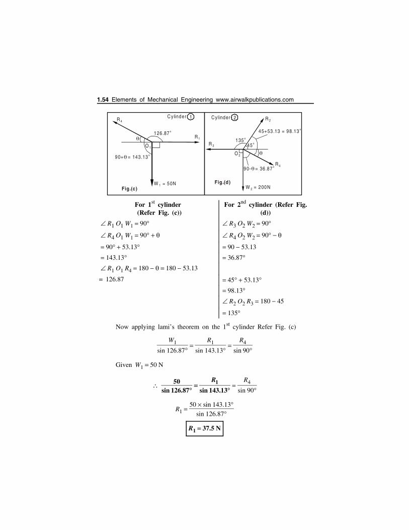
For 1st cylinder (Refer Fig. (c))

For 2nd cylinder (Refer Fig.(d))

R1 O1 W1 90 R3 O2 W2 90

R4 O1 W1 90 R4 O2 W2 90

90 53.13 90 53.13

143.13 36.87 R1 O1 R4 180 180 53.13

= 126.87 45 53.13 98.13 R2 O2 R3 180 45

135

Now applying lami’s theorem on the 1st cylinder Refer Fig. (c)

W1

sin 126.87

R1

sin 143.13

R4

sin 90

Given W1 50 N

50

sin 126.87

R1

sin 143.13

R4

sin 90

R1 50 sin 143.13

sin 126.87

R1 37.5 N

135 o

45 oR 3

R 2

R 4

W = 200N2

O 2

45+53 .13 = 98.13 o

90-= 36 .87 o

Fig.(d)

R 4

R 1126 .87 o

W = 50N1

90+= 143.13 o

C ylinder 1

Fig.(c)

O 1

C ylinder 2


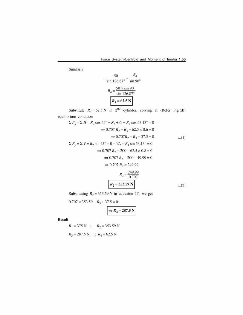
Similarly

50

sin 126.87

R4

sin 90

R4 50 sin 90sin 126.87

R4 62.5 N

Substitute R4 62.5 N in 2nd cylinder, solving at (Refer Fig.(d))

equilibrium condition

Fx H R2 cos 45 R3 O R4 cos 53.13 0

0.707 R2 R3 62.5 0.6 0

0.707R2 R3 37.5 0 ...(1)

Fy V R2 sin 45 0 W2 R4 sin 53.13 0

0.707 R2 200 62.5 0.8 0

0.707 R2 200 49.99 0

0.707 R2 249.99

R2 249.990.707

R2 353.59 N ...(2)

Substituting R2 353.59 N in equation (1), we get

0.707 353.59 R3 37.5 0

R3 287.5 N

Result

R1 375 N ; R2 353.59 N

R3 287.5 N ; R4 62.5 N


Problem 1.20: Two homogeneous spherical balls rest between two verticalwalls as shown in Fig. 2. The radius of smaller ball is 16 cm and weight is1.15 kN. The radius of the larger ball is 24 cm and its weight is 3.45 kN.The distance between the walls is 72 cm. Assuming the contact surfaces tobe smooth, determine the reactions at A, B and C.

Solution:

Given data

r1 16 cm

W1 1.15 kN

r2 24 cm

W2 3.45 kN

Distance between the walls = 72 cm

Let the point of contact of both the spheres be denoted by D.

Now, we will draw the free body diagram for both the spheres individually.

Find the inclination of both spheres, let it be inclined at .

Distance O1 to O2

r1 r2 16 24 40 cm

C

B

A

72 cm

1

2

R C

R B

R A

W 1

W 1

O 1

O 2

D

R D R Dr1

r2

12


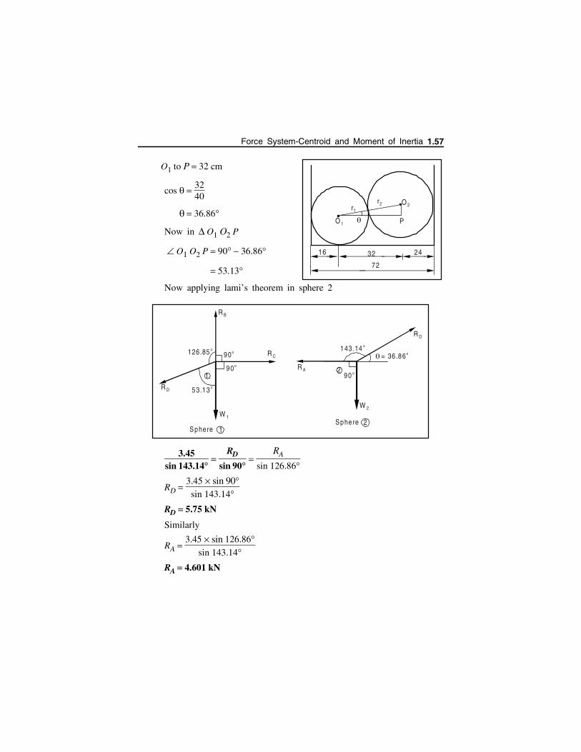
O1 to P 32 cm

cos 3240

36.86

Now in O1 O2 P

O1 O2 P 90 36.86

53.13

Now applying lami’s theorem in sphere 2

3.45sin 143.14

RD

sin 90

RA

sin 126.86

RD 3.45 sin 90

sin 143.14

RD 5.75 kN

Similarly

RA 3.45 sin 126.86

sin 143.14RA 4.601 kN

R D

R B

R C

53.13 o

126 .85 o

90o

90o

W 1

1R A

R D

90 o

143 .14 o

W 2

= 36 .86o

2

1SphereSphere 2

72

32 2416

O 1

O 2r2

r1

P


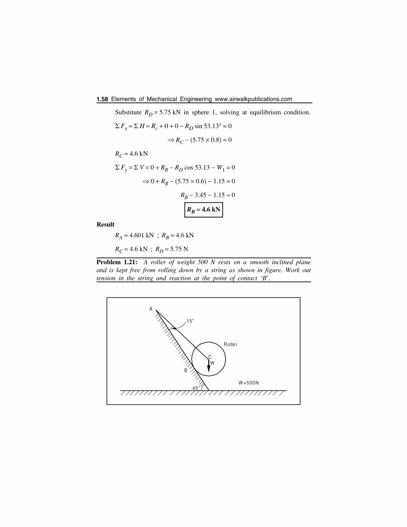
Substitute RD 5.75 kN in sphere 1, solving at equilibrium condition.

Fx H Rc 0 0 RD sin 53.13 0

RC 5.75 0.8 0

RC 4.6 kN

Fy V 0 RB RD cos 53.13 W1 0

0 RB 5.75 0.6 1.15 0

RB 3.45 1.15 0

RB 4.6 kN

Result

RA 4.601 kN ; RB 4.6 kN

RC 4.6 kN ; RD 5.75 N

Problem 1.21: A roller of weight 500 N rests on a smooth inclined planeand is kept free from rolling down by a string as shown in figure. Work outtension in the string and reaction at the point of contact ‘B’.

A

15o

R o lle r

B

W =500N45o

CW


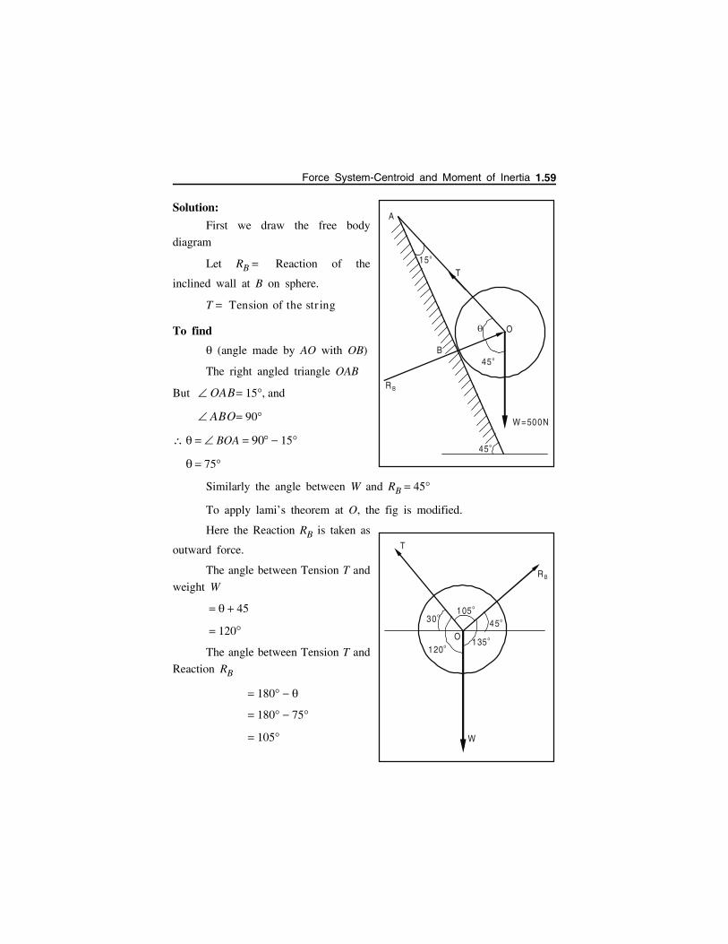
Solution:

First we draw the free body

diagram

Let RB Reaction of the

inclined wall at B on sphere.

T Tension of the str ing

To find

(angle made by AO with OB)

The right angled triangle OAB

But OAB 15, and

ABO 90

BOA 90 15

75

Similarly the angle between W and RB 45

To apply lami’s theorem at O, the fig is modified.

Here the Reaction RB is taken as

outward force.

The angle between Tension T and

weight W

45

120

The angle between Tension T and

Reaction RB

180

180 75

105

B

R B

45o

45o

W =500N

A

15o

O

T

W

T

R B

30o

45o

120o 135o

105o

O


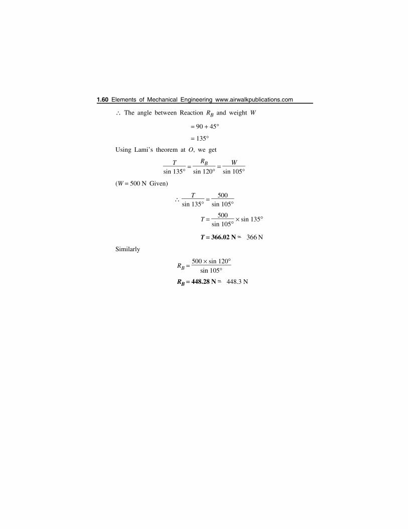
The angle between Reaction RB and weight W

90 45

135

Using Lami’s theorem at O, we get

Tsin 135

RB

sin 120

Wsin 105

(W 500 N Given)

T

sin 135

500sin 105

T 500

sin 105 sin 135

T 366.02 N ~ 366 N

Similarly

RB 500 sin 120

sin 105

RB 448.28 N ~ 448.3 N


elements of mechanical engineering - …airwalkbooks.com/images/pdf/pdf_56_1.pdf · (vi) propped...

Documents