emanuele haus dynamics of an elastic satellite with
TRANSCRIPT

Emanuele Haus
Dynamics of an elastic satellite with internal friction
Asymptotic stability vs collision or expulsion
Ledizioni LediPublishing
Emanuele Haus Department of Mathematics University of Milan Via C. Saldini n.50 20133 Milan - Italy Advisor: Dario Paolo Bambusi Department of Mathematics University of Milan Via C. Saldini 50, Milan, Italy Series Editors: Bert van Geemen, Coordinator of the PhD Program in Mathematics; Giovanni Naldi, Coordinator of the PhD Program in Mathematics and Statistics for Computational Sciences; Luca Barbieri Viale, Director of the Graduate School. Editorial Assistant: Stefania Leonardi © 2013 Emanuele Haus Open Access copy available at air.unimi.it First Edition: January 2013 ISBN 978-88-6705-067-3 All rights reserved for the print copy. For the digital copy rights please refer to air.unimi.it Ledizioni LediPublishing Via Alamanni 11 – 20141 Milano – Italy http://www.ledipublishing.com [email protected]
University of MilanDepartment of Mathematics
Graduate School in Mathematical SciencesPh.D. program in Mathematics – XXIV cycle
Dynamics of an elastic satellitewith internal friction
Asymptotic stability vs collision or expulsion
Ph.D. Thesis
AdvisorProf. Dario Paolo Bambusi
CandidateEmanuele Haus
Academic Year 2010/2011


Contents
Introduction 3
1 The classical theories: a short review 91.1 General facts . . . . . . . . . . . . . . . . . . . . . . . 91.2 Bodily tides: the Darwin-Kaula approach . . . . . . . 111.3 Physical origin of the phase lags . . . . . . . . . . . . 181.4 Our approach . . . . . . . . . . . . . . . . . . . . . . . 20
2 Asymptotic behavior of a satellite 252.1 The setting . . . . . . . . . . . . . . . . . . . . . . . . 26
2.1.1 Constitutive relations . . . . . . . . . . . . . . 282.1.2 Boundary conditions . . . . . . . . . . . . . . . 31
2.2 The Cauchy problem . . . . . . . . . . . . . . . . . . . 312.3 LaSalle’s invariance principle . . . . . . . . . . . . . . 332.4 Characterization of non-dissipating orbits . . . . . . . 38
1

CONTENTS 2
2.5 The “three outcomes” theorem . . . . . . . . . . . . . 492.5.1 Comments about the meaning of the theorem
of the three outcomes . . . . . . . . . . . . . . 54
3 Orbital stability 593.1 General setting and global rotations . . . . . . . . . . 623.2 The matrix of inertia as a function of the configuration 693.3 Planar restriction . . . . . . . . . . . . . . . . . . . . . 693.4 The gravitational interaction . . . . . . . . . . . . . . 703.5 Triaxial satellite . . . . . . . . . . . . . . . . . . . . . 75
3.5.1 Lagrangian coordinates . . . . . . . . . . . . . 763.5.2 Potential energy . . . . . . . . . . . . . . . . . 783.5.3 Kinetic energy . . . . . . . . . . . . . . . . . . 803.5.4 The reduced Lagrangian . . . . . . . . . . . . . 823.5.5 Dissipative dynamics . . . . . . . . . . . . . . . 86
3.6 Spherically symmetric satellite . . . . . . . . . . . . . 883.6.1 Adapted coordinates . . . . . . . . . . . . . . . 903.6.2 Elastic potential energy . . . . . . . . . . . . . 993.6.3 Planar restriction . . . . . . . . . . . . . . . . . 1013.6.4 Kinetic energy . . . . . . . . . . . . . . . . . . 1023.6.5 Lagrangian and reduction . . . . . . . . . . . . 1033.6.6 Dissipative dynamics . . . . . . . . . . . . . . . 1093.6.7 Multi-layer satellite . . . . . . . . . . . . . . . 110
3.7 General comments . . . . . . . . . . . . . . . . . . . . 1123.8 A direct proof of the asymptotic stability . . . . . . . 113

Introduction
In this thesis, we study the dynamics of an elastic body whose shapeand position evolve due to the gravitational forces exerted by a point-like planet whose position is fixed in the space. The first result of thethesis is that, if any internal deformation of the body dissipates someenergy, then the dynamics of the system has only three possible finalbehaviors:
(i) the satellite is expelled to infinity;
(ii) the satellite falls on the planet;
(iii) the satellite is captured in synchronous resonance.
By item (iii) we mean that the shape of the body reaches a finalconfiguration, that a principal axis of inertia is directed towards theattracting planet and that the center of mass of satellite moves on acircle of constant radius.
3
CONTENTS 4
Secondly we study the stability of the synchronous orbit. Restrict-ing to the quadrupole approximation and assuming that the body isvery rigid, we prove that such an orbit is (locally) asymptoticallystable.
Some additional results on the dynamics of the body close to thesynchronous orbit and some new kinematic results are also presentin the thesis.
The theory of bodily tides traces its origin back to the pioneeringwork by Darwin [9,10], who was actually interested in the long-timeeffects on the Earth’s rotation of the tides generated by the Moon.He studied the following situation: consider an elastic planet, whosecenter of mass is fixed in space and which rotates with a fixed angularvelocity. Then, put a pointlike satellite on a fixed Keplerian orbitaround the center of mass of the planet. As a consequence, the planetwill experience tidal distortion. If the material of the planet wereperfectly inviscid, then the planet would instantaneously reach anequilibrium configuration. To account for viscosity, Darwin assumedthat such a deformation has instead some delay called phase lag.Using also some form of the averaging principle, Darwin obtained anexpression of an effective dissipation acting on the orbital and spindegrees of freedom. His argument can also be used to deduce thestability of the 1:1 resonance in the Moon-Earth system.
Darwin’s work was subsequently generalized by Kaula [20] andmany other authors (for instance, [1, 15, 25, 30]). Critical reviews of

CONTENTS 5
the work by Darwin, Kaula and followers can be found in [11–13].In particular, Kaula has developed a theory based on the use of theKeplerian orbital elements in order to describe the tidal forces actingon the body and the corresponding reactions and phase lags. Thisallowed him to obtain much more effective results.
In most of the subsequent studies on the spin orbit interactionin the dynamics of a satellite, the satellite is treated as a rigid bodysubject to the effective dissipative force and, moreover, most of thetimes the orbit of the center of mass is fixed and the evolution ofthe spin degrees of freedom is studied. The papers [4–6] take exactlythis approach. Here some KAM type results have been obtained andfurthermore analytic and numerical techniques have been used inorder to explain the spin orbit resonance in systems like Earth-Moonor Sun-Mercury. In particular some remarkable explanation on the3:2 resonance observed in the Sun-Mercury system has been given.
Recently Efroimsky [12] revisited the theory of Darwin and Kaula;by using continuum mechanics he computed explicitly the expressionof the phase lags to be inserted in the equation of motion.
As described above, the point of view of this thesis is much morefundamental: we assign neither the shape of the body nor its orbit,instead we consider the equations of elasticity (governing the inter-nal dynamics of the satellite) coupled with the Newton equationsgoverning the orbital and spin degrees of freedom and study the cor-responding dynamics. We try to make as few assumptions as possible

CONTENTS 6
in order to understand if a general behavior appears, independentlyof, possibly all, the specific features of the model.
The main result is the one explained at the beginning of this ab-stract. The only assumption needed to get such a result pertainsthe nature of the dissipation acting on the internal degrees of free-dom. To state it, denote by σ the stress tensor and by ε the straintensor related to the elastic configuration of the satellite. Then, theassumption is that the constitutive relation has the form
σ = F (ε, ε) .
In particular, we assume that the stress at a given time is only func-tion of the strain and of its time derivative at that fixed time, andthat there are no memory effects.
The proof of the main result makes use of the so-called LaSalle’sprinciple [23], which is a generalization of Lyapunov theorem to thecase where there is a nontrivial set N on which the Lie derivative ofa Lyapunov function vanishes. LaSalle’s principle ensures that, if thephase space is compact, then any orbit approaches the largest invari-ant set contained in N . For the proof we first reduce to the compactcase by eliminating escaping and colliding orbits, then we show thatthe above invariant set is constituted by synchronous orbits.
Afterwards we study the stability of the synchronous resonance.Surprisingly enough such a study is much more complicated thanthe previous global one. This is essentially due to the fact that tothis end one has to explicitly write the Lagrangian of the system

CONTENTS 7
and to study the corresponding equations. So, for this study wereduce to the quadrupole approximation, and then introduce suitablecoordinates in the configuration space. In such an approximation thegravitational potential turns out to be a function of the position ofthe center of mass of the body, of its moments of inertia and of theorientation of the principal axes of inertia. So, it is natural to tryto use such functions as coordinates in the configuration space. Weprove that this is possible, but to this end we have to study separatelytwo different situations: (1) the body has a rest configuration in whichit is a sphere, (2) it has a rest configuration in which it is a triaxialbody. In case (2) the analysis is simple, while in the other case theanalysis is more difficult and requires the use of some properties ofthe spaces obtained as the quotient of a Hausdorff space with respectto the action of a finite group. The conclusion is that the wantedcoordinates are a 24 fold covering of the configuration space.
Then exploiting some general principles of mechanics we write theLagrangian of the system in the considered coordinates and provethe orbital stability of the synchronous orbit. Asymptotic stabilityfollows by exploiting the global stability result.
It is worth mentioning that in the case of a spherical body theresult does not imply that the body eventually stops deforming, butonly that its shape is such that a principal axis of inertia alwayspoints towards the planet. The axes of inertia could slide indefinitelyin the body.

CONTENTS 8
Chapter 1 of the thesis is devoted to a brief review about the ex-isting theories which concern bodily tides and spin-orbit resonances.
Chapter 2 and Chapter 3 contain the original contribution toknowledge that is present in this PhD. thesis. Chapter 2 is devoted tothe proof of the main result of this thesis, i.e. the fact that a satellitemust escape, collide or get trapped in the synchronous resonance.The content of Chapter 2 is summarized in the paper
• E. Haus. Asymptotic behavior of an elastic satellite with fric-tion, preprint.
Chapter 3 contains the proof of the orbital stability of the syn-chronous resonance. The case of a triaxial body is studied in
• D. Bambusi and E. Haus. Stability of the synchronous reso-nance for the dynamics of a viscoelastic satellite, preprint.
The result for a body with spherical symmetry is obtained in
• D. Bambusi and E. Haus. Asymptotic stability of spin orbitresonance for the dynamics of a viscoelastic satellite,http://arxiv.org/abs/1012.4974, submitted.

Chapter 1
The classical theories: a shortreview
1.1 General facts
It has always been a well known fact that the Moon always showsthe same face to the Earth. This happens because the period of rota-tion of the Moon about its axis equals the period of revolution of theMoon around the Earth. The fact that the two periods are exactlyequal already suggests that it should not be a coincidence. Moreover,in the last decades more and more data have become available thanksto explorations of the Solar system, which have shown that most ma-jor satellites in the Solar system always point the same face towards
9

CHAPTER 1. CLASSICAL THEORIES: A SHORT REVIEW 10
their mother planet. The heuristic explanation for this phenomenonhas been known for a very long time. The gravitational field gener-ated by a celestial body is not constant in space. Since even solidbodies (like many satellites are, at least as a first approximation)are slightly deformable, the satellite experiences some deformationdue to the non-constancy of the gravitational field generated by theplanet. In particular, the satellite gets slightly stretched towards theplanet, such an elongation making the situation where the satellitealways shows the same face to the planet physically stable. Such adeformation of the satellite is originated by the same type of effectwhich generates ocean tides on the Earth. For this reason, the sit-uation in which a celestial body always shows the same face to thebody it orbits is often referred to as “tidal locking”. In a wider con-text, one may be interested in the so-called spin-orbit resonances. Aspin-orbit resonance occurs whenever the ratio between the period ofrotation and the period of revolution of a given celestial body is arational number. The situation of tidal locking therefore correspondsto the 1:1 spin-orbit resonance (and zero inclination of the axis ofrotation), also called synchronous resonance for obvious reasons. Inthe Solar system, the main body which is in a spin-orbit resonancedifferent from the synchronous one is Mercury, which is caught in a3:2 resonance around the Sun, meaning that Mercury’s orbital periodequals three halves its rotational period.
If, on the one side, the heuristic explanation of the phenomenon
CHAPTER 1. CLASSICAL THEORIES: A SHORT REVIEW 11
of tidal locking is rather simple, on the other side the rigorous math-ematical investigation is very complicated. In fact, what in principleone should do is to study a complicated system of partial differentialequations describing the evolution of the internal configuration of thebodies, coupled with ordinary differential equations describing theevolution of the orbital and rotational parameters. Such an investi-gation is made even more complicated by the fact the inner structureof celestial bodies is often very complicated and never known withabsolute precision.
Since it is too difficult to find the solutions to the complete prob-lem of motion of a deformable body in a gravitational field, the ex-isting theories of bodily tides always make use of some relevant ap-proximations. In the next section, we will make a brief review ofthe history of the classical theory of bodily tides. The huge amountof work which has been spent on the subject makes it impossible toperform a complete review, so we will focus on the main aspects ofthe theory, in order to clarify the distinction between the classicalapproach to the theory of bodily tides and the approach that we willfollow in the present PhD. thesis.
1.2 Bodily tides: the Darwin-Kaula approach
In this section we give a brief description of the classical Darwin-Kaula theory of bodily tides, which has set the basis on which manyauthors ( [14–17, 21, 22, 25, 27–29, 32, 34]) have worked in the last

CHAPTER 1. CLASSICAL THEORIES: A SHORT REVIEW 12
decades, in order to understand the main effects of the tidal frictionin the Solar System. For a much more detailed review of Darwin’stheory, see [13], whose notation we will follow in this section. Acritical review of the different techniques which have been developedin order to explore the consequences of torques due to bodily tidescan be found in [11].
When developing his theory of tides, Darwin was actually inter-ested in studying the long-time effects on the Earth’s rotation of thetides generated by the Moon.
The situation studied by Darwin ( [9,10]) is the following: considera central, deformable body of mass m, whose center of mass is at theorigin, and an outer pointlike mass M , which is responsible for thedeformation of m. At first, m is considered to be a homogeneous andperfect inviscid fluid, which assumes the equilibrium configurationunder its own gravity and the external gravitational forces due toM ,which generate tides onm. Let r = (r, θ, ϕ) (spherical coordinates) bethe vector representing the position ofM . If now we neglect the polarflattening due to the rotation of m and we consider only the mainterm of the tide generating potential (i.e., if we neglect terms beyondquadrupole in the multipole expansion of the potential generated byM), the equilibrium configuration is a Jeans spheroid (an ellipsoidwhose three semi-axes satisfy A > B = C), whose semi-major axis Ais directed towards M and whose prolateness is given by
ε := A
B− 1 = 15
4M
m
(R
r
)3, (1.2.1)

CHAPTER 1. CLASSICAL THEORIES: A SHORT REVIEW 13
where R is the mean radius of m (see [33]). We note that Darwinused the Jeans spheroid as equilibrium configuration, because at thattime Love’s theory [24] was not available yet. Using Love’s theory, itis possible to include also polar flattening in the equilibrium config-uration [7], but the results that one obtains are essentially the sameas for the Jeans spheroid.
Then consider an arbitrary point r∗ = (r∗, θ∗, ϕ∗) in space. Thegravitational potential generated by the prolate spheroid of equation(1.2.1) is given by
U(r∗) = −Gmr∗− kfGMR5
2r3r∗(3 cos2 Ψ− 1) , (1.2.2)
where Ψ is the angle between r and r∗ and kf is the parameter thatin the modern language is called fluid Love number. In the case of ahomogeneous sphere, kf = 3
2 .In Darwin’s theory, the assumption is made that the body M
orbits m on a fixed Keplerian orbit of semi-major axis a, eccentric-ity e and inclination I. Then, the position r of M is a function ofthe orbital elements. Therefore, one can write the expression of thepotential generated by the deformed m as a function of the orbitalelements of M . Define the tide raising potential as
U02 (r∗) := U(r∗)− Gm
r∗.
In terms of the mean anomaly l, which is a linear function of time

CHAPTER 1. CLASSICAL THEORIES: A SHORT REVIEW 14
(l = nt+ l0), one has, to second order in e and I,
U02 = −3kfGMR5
4a3r∗3
[−2
3 − e2 +(
1 + 32e
2 − 12S
2)P 2+
+(
1− 52e
2 − 12S
2)P 2 cos(2ϕ∗ − 2l − 2ω) +
+72eP
2 cos(2ϕ∗ − 3l − 2ω) +
−12eP
2 cos(2ϕ∗ − l − 2ω) + 172 e
2P 2 cos(2ϕ∗ − 4l − 2ω) +
−(2− 3P 2)e cos l −(
3− 92P
2)e2 cos 2l +
+QS[sinϕ∗ − sin(ϕ∗ − 2l − 2ω)] +
+12P
2S2[cos 2ϕ∗ + cos(2l + 2ω)] (1.2.3)
where we have used the notation S = sin I, P = sin θ∗, Q = sin 2θ∗
and we have denoted by ω the argument of the periapsis. Observethat such a tide raising potential is a function of time through l.
If now one is interested in the tide raising effect of the potentialU0
2 on the central body m, one has to think of the point r∗ as co-rotating with m, i.e. such that r∗ and θ∗ are constant, while thelongitude ϕ∗ is given by ϕ∗ = Ωt+ ϕ∗0, Ω being the angular velocityof rotation of the body m.
In this way, the expression (1.2.3) becomes a function of timethrough both l and ϕ∗, where one can recognize the sum of periodicterms with nine different frequencies.
There comes the main idea in Darwin’s work: the phase lag. Upto now, we have assumed that the deformable body were perfectly

CHAPTER 1. CLASSICAL THEORIES: A SHORT REVIEW 15
inviscid and that it instantaneously reached the equilibrium config-uration. Darwin, in order to take into account the effects related toviscosity, made the following assumption: the deformable body reactsto the tidal action, but it does with some delay due to its viscosity. Inparticular, since the potential U0
2 is the sum of time-periodic termswith different frequencies, a specific delay is added for each periodicterm. If Φi is a generic time-periodic argument, then the procedureconceived by Darwin consists in replacing Φi with the “delayed” termΦi−εi, and then considering the first order approximation in the lagsin the following way:
cos(Φi − εi) = cos Φi + εi sin Φi (1.2.4)
sin(Φi − εi) = sin Φi − εi cos Φi . (1.2.5)
Then, plugging the lags into the expression of U02 , one finds that
the quardupole term of the gravitational potential becomes
U2 = U02 + Ulag , (1.2.6)
where the correction Ulag due to the delayed response of the de-

CHAPTER 1. CLASSICAL THEORIES: A SHORT REVIEW 16
formable body is given by1
Ulag = −3kfGMR5
8a3r∗3[P 2ε0(2− 5e2 − S2) sin(2ϕ∗ − 2l − 2ω)+
+eP 2(7ε1 sin(2ϕ∗ − 3l − 2ω)− ε2 sin(2ϕ∗ − l − 2ω) +
+17e2P 2ε3 sin(2ϕ∗ − 4l − 2ω) + P 2S2ε4 sin(2ϕ∗) +
−eε5(4− 6P 2) sin l − 3e2ε6(2− 3P 2) sin(2l) +
+P 2S2ε7 sin(2l + 2ω) +
+ 2QS(ε8 cos(ϕ∗ − 2l − 2ω)− ε9 cosϕ∗)] . (1.2.7)
Then the field associated to tidal forces generated by the deformedbody in any point of the space can be easily calculated as the gradientof the gravitational potential U2 = U2
0 + Ulag. As one expects, thecomputation of the gradient of U2
0 gives a purely radial field, sincein the absence of lags one would have an equilibrium configurationwhich does not involve any torque.
Then, evaluating the so-obtained tidal field in the point r =(r, θ, ϕ) where the body M is placed, and multiplying it by its massM , one has the tidal force F acting on M , generated by the tideraised on m by M itself.
Because of the presence of the lags, the tidal force F is not aligned1When considering the effects of friction, we should also have replaced the
static Love number kf with its dynamical counterparts, in order to take intoaccount some attenuation of the tidal response due to viscosity. Anyway, forsimplicity, we are neglecting this aspect in this short summary of Darwin’stheory.

CHAPTER 1. CLASSICAL THEORIES: A SHORT REVIEW 17
with r, a fact which generates a non-zero torque
M = r× F .
This is actually the machinery for obtaining expressions of thetidal forces and torques, in Darwin’s theory. From these expressions,using conservation laws and averaging the torque < M > over oneorbital period, one can get expressions for the secular variations ofthe orbital elements of M and of the rotation of m, and expressionsfor the energy dissipation.
We do not enter the details of these calculations, which are verywell explained in [13]. We limit ourselves to writing down the expres-sions obtained through Darwin’s theory. Denoting by C the momentof inertia related to the axis of rotation of m, by J the inclinationof the axis of rotation of m and by E the mechanical energy of thesystem, the following expressions are obtained.
< Ω >= 3kfGM2R5
8Ca6 [4ε0+e2(−20ε0+49ε1+ε2)+2S2(−2ε0+ε8+ε9)](1.2.8)
< J >= 3kfGM2R5
4CΩa6 S(ε0 + ε8 − ε9) (1.2.9)
< n > = −3n2a < a >= −9n2kfMR5
8ma5
[4ε0 − 4S2(ε0 − ε8)
]+
−9n2kfMR5e2
8ma5
(20ε0 −
1472 ε1 −
12ε2 + 3ε5
)(1.2.10)

CHAPTER 1. CLASSICAL THEORIES: A SHORT REVIEW 18
< E > = 3kfGM2R5
8a6
n[4ε0 − 4S2(ε0 − ε8)
]+
+ne2(−20ε0 + 1472 ε1 + 1
2ε2 − 3ε5) +
−Ω[4ε0 + e2(−20ε0 + 49ε1 + ε2) +
+ 2S2(−2ε0 + ε8 + ε9)]
(1.2.11)
< e >= −3nekfMR5
8ma5
(2ε0 −
492 ε1 + 1
2ε2 + 3ε5
)(1.2.12)
< I >= 3nkfSMR5
4ma5 (−ε0 + ε8 − ε9) . (1.2.13)
Many decades after Darwin, Kaula [20] made a remarkable gener-alization of Darwin’s work. Kaula computed tidal forces and torquesfollowing Darwin’s approach; however, whereas Darwin stopped toquadrupole terms in the multipole expansion of the tidal potential,Kaula was able to deduce an impressive formula (see [11], equations(20) and (21)) expressing the complete multipole expansion of thetidal potential in terms of the orbital elements of M . Kaula’s contri-bution has been so relevant that the theory which consists in intro-ducing the phase lags in Kaula’s expression of the tidal potential anddeducing dynamical consequences, in a way similar to that explainedabove, is commonly referred to as Darwin-Kaula theory.
1.3 Physical origin of the phase lags
The classical Darwin-Kaula approach has the advantage of being verygeneral, since no assumptions are done about the values that must
CHAPTER 1. CLASSICAL THEORIES: A SHORT REVIEW 19
be given to the phase lags εi. However, in order to make a rigorousphysical theory of bodily tides, starting from first principles, oneshould do the following: (i) understand the physical origin of thephase lags, (ii) study a realistic model of deformable body and deducethe expressions for the phase lags as a function of the deformablebody’s rheology.
In order to understand the origin of the phase lags, it is usefulto think of the analogy with a damped harmonic oscillator, witha periodic external forcing. If one has a damped oscillator with asinusoidal forcing of the type
x+ 2ζω0x+ ω02x = A sin(ωt) , (1.3.1)
then the solution is the sum of a transient solution, which dependson the initial conditions and goes exponentially to zero, and a steadystate solution, which is independent of the initial conditions. Thesteady state is
x(t) = A
Bωsin(ωt+ φ) , (1.3.2)
where
B =√
(2ω0ζ)2 + 1ω2 (ω02 − ω2)2
andφ = arctan
( 2ωω0ζ
ω2 − ω02
).
As we can see from these expressions, the steady state is an oscil-lation which has the same frequency as the external forcing, but isresponding with a delay φ.

CHAPTER 1. CLASSICAL THEORIES: A SHORT REVIEW 20
In this trivial example, the harmonic oscillator plays the role ofthe deformable body close to its equilibrium configuration, the ex-ternal forcing corresponds to the disturbing potential generated bythe point mass M , which in the Darwin-Kaula approach is actuallya sum of infinitely many time-periodic terms (since M revolves peri-odically on a Keplerian orbit), and the phase shift φ plays the role ofthe phase lags of the Darwin-Kaula theory.
In [12] a very detailed explanation of the origin of phase lags isgiven, and, using techniques from continuum mechanics, the expres-sions of the phase lags for some relevant rheological models (namelythe Maxwell model and the Andrade model) are obtained.
1.4 Our approach
The applications that were developed starting form the Darwin-Kaulaapproach turned out to be an effective tool for achieving a very goodunderstanding of many aspects of tidal torques and tidal dissipa-tion in the Solar system. However, from a mathematician’s point ofview, in such an approach there are many assumptions that need tobe justified in a rigorous way. Most notably, the whole mechanismof deduction of forces and torques in then model relies on the as-sumption that the motion occurs on a fixed Keplerian orbit. Thisis certainly “almost true” for all major bodies in the Solar system,within certain time scales. However, there is no a-priori reason toexpect that such an approximation is good when working on much

CHAPTER 1. CLASSICAL THEORIES: A SHORT REVIEW 21
longer time scales, for instance comparable to the lifespan of the So-lar system. Even computer simulations [8] seem to suggest that onvery long time scales the dynamics of the Solar system is more likelyto appear irregular and chaotic rather than steady and ordered.
For this reason, in the present thesis, we deal the problem ofstability of the synchronous resonance within a much more funda-mental setting. Since we are interested in studying the asymptoticstability over an infinite amount of time, we need to get rid of thoseapproximations which, despite being very good approximations ontime scales which are not too long, are inadequate for studying thebehavior of celestial bodies over infinite times. Since we approachthe problem of stability of the synchronous resonance, and since typ-ically in the Solar system such a behavior is exhibited by satellitesorbiting their mother planet, we are interested in proving that thetidal deformation of the satellite itself stabilizes the synchronous res-onance. Therefore, since in the planet-satellite system the satellitehas a smaller mass (usually much smaller), we consider a differentsetting from the Darwin-Kaula one already in the fact that in ourmodel the pointlike mass is supposed to be immobile, while the de-formable body (which models the satellite) is supposed to be free tomove in space. What is most important is that we will not make anyassumption about the motion of the center of mass of the satellite(except the fact that the motion is planar, and only for the results oforbital stability of Chapter 3). In Chapter 3, we will make the pla-

CHAPTER 1. CLASSICAL THEORIES: A SHORT REVIEW 22
nar restriction, which actually corresponds to an assumption of zeroinclination of the axis of rotation of the satellite. However, we wouldlike to point out that such an assumption has been done in this thesiswith the only aim of simplifying the form of the equations of motionand consequently simplifying the study of the properties of the dy-namical system. There is no obstruction in using the same formalismthat we have developed in Chapter 3 for a system where the planarrestriction has been removed. On the contrary, the study of such acomplete 3-dimensional system is a very natural future developmentof the results obtained in this thesis. Another point is that, by con-sidering the planet as a pointlike mass, we actually neglect the effectsof tidal deformation and dissipation in the planet: again, there is noformal obstruction to the application of our techniques for the studyof a system consisting of two deformable bodies. The introductionof a deformable planet would only result in a complication of theequations of motion.
It is worth making some more comments on the existing litera-ture, in order to better explain why the results that we obtain are notin contrast with the already existing ones. In particular, in [4–6] a se-ries of studies is conducted about the stability of spin-orbit resonance.The point of view that is taken here is the following: consider a rigidbody, whose center of mass revolves around an immobile pointlikemass on a fixed Keplerian orbit. The rotational motion of this rigidbody has zero inclination and is subject to some effective friction,

CHAPTER 1. CLASSICAL THEORIES: A SHORT REVIEW 23
which modifies the speed of rotation of the satellite and which is cal-culated according to some applications of the classical Darwin-Kaulatheories. In such a context, the stability of spin-orbit resonances isinvestigated, and evidence is found that the eccentricity of the orbit isa very relevant parameter in the selection of the spin-orbit resonancein which the satellite might get trapped. For instance, on a circularorbit the satellite will fall on a 1:1 resonance, while with eccentricitye = 0.205 (the eccentricity of Mercury) the satellite is quite likely tofall into the 3:2 resonance, which is (locally) asymptotically stable.As we have anticipated in the introduction, the main result of thisthesis, which is explained in Chapter 2, rules out the possibility thata non-synchronous resonance is asymptotically stable. Where is thecontradiction? Actually, there is no contradiction. The method usedin [4–6] imposes that the satellite moves on a fixed Keplerian orbit.The vanishing of the effective friction in this model corresponds tothe fact that < Ω >= 0, in terms of Darwin’s theory explained above.Anyway, it may very well happen that Ω = 0, but that, at the sametime, secular changes in the parameters of the Keplerian orbit occur.After a long time, the orbit will have changed and there is no reasonfor which, on the new orbit, < Ω >= 0 should hold again. Therefore,the fact that a 3:2 resonance appears as an equilibrium in a modelwith fixed orbit means that, in a model where the orbit parametersare left free to vary, the 3:2 resonance will be stable for a long time,but not for an infinite time.

CHAPTER 1. CLASSICAL THEORIES: A SHORT REVIEW 24
Of course, a very interesting point is the validation of the Darwin-Kaula theory. In particular, it would be very relevant to be able togive an estimate of the time scale of validity of the classical theories ofbodily tides. In our language, the approximation by Darwin consistsin the assumption that the degrees of freedom corresponding to theconfiguration of the deformable body adapt themselves with a delaygiven by the phase lags. It is very natural to think of this problemas an application of perturbation theory. We are currently workingat the connection of our model with the Darwin-Kaula theories andwhat we are trying to prove is that our model reduces to the one byDarwin and Kaula at the second order in perturbation theory, thesmall parameter being the kinetic energy associated to the bodilydeformations.

Chapter 2
Asymptotic behavior of asatellite
In this chapter we will refer to a dynamical system consisting of:
(i) a pointlike mass M (which we will sometimes call “planet”),whose space coordinates are fixed;
(ii) an elastic body with internal friction, of any shape, free to movein space (and to orbit the pointlike mass M); we will call thisextended body “satellite”.
In order to deal with the point (ii), we must set our study intothe context of the theory of elasticity.
25
CHAPTER 2. ASYMPTOTIC BEHAVIOR OF A SATELLITE 26
2.1 The setting
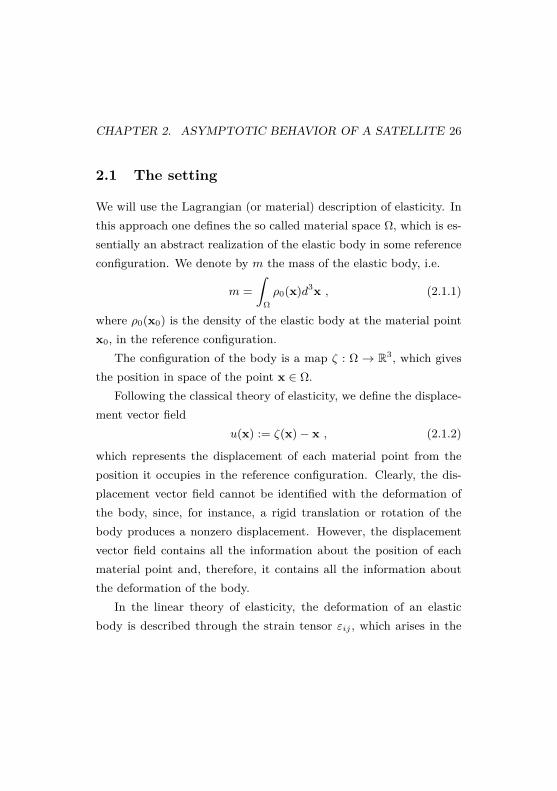
We will use the Lagrangian (or material) description of elasticity. Inthis approach one defines the so called material space Ω, which is es-sentially an abstract realization of the elastic body in some referenceconfiguration. We denote by m the mass of the elastic body, i.e.
m =∫
Ωρ0(x)d3x , (2.1.1)
where ρ0(x0) is the density of the elastic body at the material pointx0, in the reference configuration.
The configuration of the body is a map ζ : Ω → R3, which givesthe position in space of the point x ∈ Ω.
Following the classical theory of elasticity, we define the displace-ment vector field
u(x) := ζ(x)− x , (2.1.2)
which represents the displacement of each material point from theposition it occupies in the reference configuration. Clearly, the dis-placement vector field cannot be identified with the deformation ofthe body, since, for instance, a rigid translation or rotation of thebody produces a nonzero displacement. However, the displacementvector field contains all the information about the position of eachmaterial point and, therefore, it contains all the information aboutthe deformation of the body.
In the linear theory of elasticity, the deformation of an elasticbody is described through the strain tensor εij , which arises in the
CHAPTER 2. ASYMPTOTIC BEHAVIOR OF A SATELLITE 27
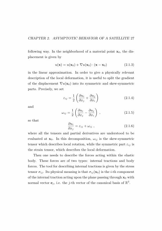
following way. In the neighborhood of a material point x0, the dis-placement is given by
u(x) = u(x0) +∇u(x0) · (x− x0) (2.1.3)
in the linear approximation. In order to give a physically relevantdescription of the local deformation, it is useful to split the gradientof the displacement ∇u(x0) into its symmetric and skew-symmetricparts. Precisely, we set
εij = 12
(∂ui∂xj
+ ∂uj∂xi
)(2.1.4)
andωij = 1
2
(∂ui∂xj− ∂uj∂xi
), (2.1.5)
so that∂ui∂xj
= εij + ωij , (2.1.6)
where all the tensors and partial derivatives are understood to beevaluated at x0. In this decomposition, ωij is the skew-symmetrictensor which describes local rotation, while the symmetric part εij isthe strain tensor, which describes the local deformation.
Then one needs to describe the forces acting within the elasticbody. These forces are of two types: internal tractions and bodyforces. The tool for describing internal tractions is given by the stresstensor σij . Its physical meaning is that σij(x0) is the i-th componentof the internal traction acting upon the plane passing through x0 withnormal vector ej , i.e. the j-th vector of the canonical basis of R3.

CHAPTER 2. ASYMPTOTIC BEHAVIOR OF A SATELLITE 28
Finally, we denote by f the vector field of body forces per unitmass acting upon the elastic body.
Imposing the conservation of linear momentum, one gets
ρ∂2ui∂t2
= ρfi + ∂
∂xjσij , (2.1.7)
which is the general equation of motion in the Lagrangian descriptionof continuum mechanics. Here, ρ(x) is the actual density at the pointx when the body is deformed. Because of the conservation of mass,ρ is a function of the configuration through
ρ(x) = ρ0(x)det ∂ζ
∂x (x). (2.1.8)
These equations, of course, are largely underdetermined unlessone specifies:
(i) the relation between the displacement vector u and the stresstensor σ;
(ii) the boundary conditions on the surface of the elastic body.
2.1.1 Constitutive relations
Extended bodies of different materials behave in a different way whena stress is applied. In particular, varying the material, the same loadof applied stress can produce different deformations. Such mechanicalproperties are specified by the so-called constitutive relations, which

CHAPTER 2. ASYMPTOTIC BEHAVIOR OF A SATELLITE 29
give the connection between the stress tensor σ(= σ(x)) and thestrain tensor ε.
In the theory of linear elasticity, the stress tensor is assumed tobe a linear function of the strain, so that, in the purely elastic case,we have
σ = σel = Bε , (2.1.9)
where B is a linear operator, which may depend on the material pointx if the body is not homogeneous.
When internal friction is considered, one has to take into accountviscous effects and the stress tensor is no more a function of the strainonly, since it depends also on the time derivative of the strain ε. Asfor the elastic stress, in the linear theories the viscous stress is givenby
σvisc = Aε , (2.1.10)
where, again, A is a linear operator which may depend on the mate-rial point x.
A simple possibility, when dealing with materials which exhibitboth an elastic and a viscous behavior, is to assume that the totalstress is simply the sum of the elastic and the viscous one, i.e.
σ = σel + σvisc = Bε+ Aε . (2.1.11)
Actually, in order to prove our result, we need not assume that(2.1.11) holds. Instead, we will make the following assumption.
CHAPTER 2. ASYMPTOTIC BEHAVIOR OF A SATELLITE 30
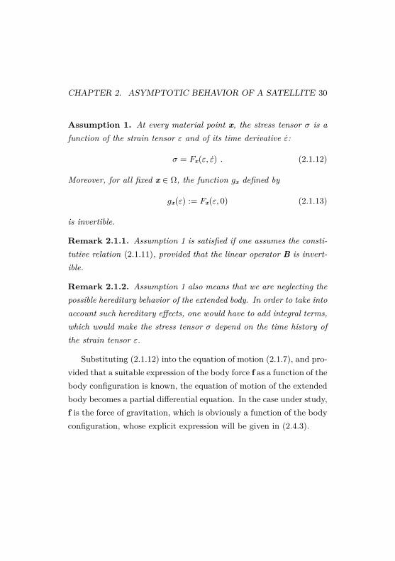
Assumption 1. At every material point x, the stress tensor σ is afunction of the strain tensor ε and of its time derivative ε:
σ = Fx(ε, ε) . (2.1.12)
Moreover, for all fixed x ∈ Ω, the function gx defined by
gx(ε) := Fx(ε, 0) (2.1.13)
is invertible.
Remark 2.1.1. Assumption 1 is satisfied if one assumes the consti-tutive relation (2.1.11), provided that the linear operator B is invert-ible.
Remark 2.1.2. Assumption 1 also means that we are neglecting thepossible hereditary behavior of the extended body. In order to take intoaccount such hereditary effects, one would have to add integral terms,which would make the stress tensor σ depend on the time history ofthe strain tensor ε.
Substituting (2.1.12) into the equation of motion (2.1.7), and pro-vided that a suitable expression of the body force f as a function of thebody configuration is known, the equation of motion of the extendedbody becomes a partial differential equation. In the case under study,f is the force of gravitation, which is obviously a function of the bodyconfiguration, whose explicit expression will be given in (2.4.3).

CHAPTER 2. ASYMPTOTIC BEHAVIOR OF A SATELLITE 31
2.1.2 Boundary conditions
In order to have a chance to obtain a well-posed problem, one has toadd suitable boundary conditions to the equation (2.1.7).
For the study of our problem, the most natural thing is to imposethe free-surface boundary condition. This means that, on the surfaceof the extended body, the component of the internal traction normalto the surface of the body vanishes.
Denoting by nx the exterior normal to the surface ζ(∂Ω) at thepoint ζ(x) ∈ ζ(∂Ω), we therefore impose the following boundarycondition.
For all x ∈ ∂Ω,σ · nx = 0 . (2.1.14)
2.2 The Cauchy problem
In the previous section, we have introduced the equation of motion(2.1.7) of continuum mechanics, which, in particular, holds for themotion of an elastic body. The natural subsequent step would bethat of searching for solutions to (2.1.7) (together with boundary andinitial conditions) in a suitable function space. In order to discussdynamics, one should in principle prove an existence and uniquenesstheorem for the solutions to the Cauchy problem and, in order to useenergy conservation (or dissipation) to prove dynamical properties,one should also prove that the dynamics is well-posed in the energy

CHAPTER 2. ASYMPTOTIC BEHAVIOR OF A SATELLITE 32
space, a fact which is in general unknown. To this end, we remarkthat, for a given state of the system, which is individuated in thephase space by the configuration of the body and by its velocityfield, the energy is given by a suitable functional, which has thestructure E(u, u) = Ekin(u;u) + Epot(u). The potential energy, inits turn, has the structure Epot(u) = Eg(u) +Esg(u) +Eel(u), whereEg is the potential energy of the extended body in the gravitationalfield generated by M , Eg is the energy of self-gravitation and Eel isthe elastic energy of deformation. In general, the elastic energy is anonlinear function of the strain tensor ε = εij3i,j=1:
Eel(u) =∫
Ωf(ε)d3x . (2.2.1)
In the linear theories of elasticity, this reduces to
Eel(u) =∫
Ω
3∑i,j,k,l=1
Bijklεijεkld3x , (2.2.2)
where Bijkl are the elements of the stiffness tensor.In this thesis, we will not enter such a kind of mathematical prob-
lems, so we will simply assume these well-posedness properties.
Assumption 2. There exists a function space X such that:

CHAPTER 2. ASYMPTOTIC BEHAVIOR OF A SATELLITE 33
(i) the Cauchy problem given by the equationsρ ∂
2ui∂t2 = ρfi + ∂
∂xjσij x ∈ Ω
σ · nx = 0 x ∈ ∂Ωu(0) = u0
u(0) = v0
(2.2.3)
admits a unique solution for all initial data (u0, v0) ∈ X.
(ii) The energy functional E(u, v) (as well as Ekin(u;u), Eg(u),Esg(u) and Eel(u)) and its Lie derivative d
dtE(u, v) along the
flow of (2.2.3) are defined for all (u, v) ∈ X and the inequality
d
dtE(u, v) ≤ 0 (2.2.4)
is satisfied for all (u, v) ∈ X.Moreover, in (2.2.4) the equality holds if and only if the sym-metric part of the gradient of v vanishes. This implies thatddtE(u, u) = 0 if and only if the time rate of change of the
deformation vanishes, i.e. if and only if ε = 0.
2.3 LaSalle’s invariance principle
In order to study the dynamics of the system, we will make useof the so-called LaSalle’s invariance principle. LaSalle’s principle isa refinement of the classical Lyapunov’s theorem, which allows oneto prove results of asymptotic stability in presence of a Lyapunovfunction E satisfying a nonstrict inequality of the type E ≤ 0.

CHAPTER 2. ASYMPTOTIC BEHAVIOR OF A SATELLITE 34
In order to give a formulation of this principle, we now fix somenotation and recall some basic facts and definitions.
Letx = f(x) x ∈ X (2.3.1)
be a system of differential equations. We denote by ϕ the flow of(2.3.1), i.e. ϕ(t,x0) is the value, at the time t of the solution to(2.3.1) with initial datum x0. The flow is a priori well-defined onlylocally in time; however, there may be initial points for which the flowis well-defined for all times, or at least for all positive times. If anorbit is defined for all positive times, then one can investigate aboutthe behavior of the orbit, as t → +∞, which involves the definitionof ω-limit.
Definition 2.3.1. Let γ be the orbit of (2.3.1) with initial conditionx(0) = x0. A point y is said to be an ω-limit point of γ if there existsa sequence of times tn → +∞ such that
limn→+∞
ϕ(tn, x) = y . (2.3.2)
Definition 2.3.2. The ω-limit set of an orbit γ is defined as theunion of all the ω-limit points of γ.
When trying to prove results of stability, one has to guaranteethat the ω-limit of the considered orbits is non-empty. To this end,some compactness assumption is needed. Then, the classical versionof LaSalle’s principle may be enunciated as follows:

CHAPTER 2. ASYMPTOTIC BEHAVIOR OF A SATELLITE 35
Theorem 2.3.3 (LaSalle’s invariance principle). Let K be a compactsubset of the phase space X. Suppose that E is a real-valued smoothfunction defined on K, whose Lie derivative satisfies E(x) ≤ 0 forall x ∈ K. Let M be the largest invariant set contained in N :=
x ∈ K|E(x) = 0. Then the ω-limit of every orbit which remains
within K for t > 0 is a non-empty subset of M , which implies thatsuch an orbit is asymptotic to M .
We remark that the fact that the ω-limit is an invariant set underthe flow of the system of differential equations is a standard fact,since it is a simple consequence of the group property of the flow.LaSalle’s principle guarantees that it must also be a set where theLie derivative of the function E vanishes. If one thinks of E as theenergy of a system with dissipation, the consequence of the invarianceprinciple is that the dynamics will lead to an asymptotic situationwhere no dissipation is present.
Proof. (LaSalle’s invariance principle) Let γ := ϕ(t,x0)|t > 0 bea forward orbit, contained in the compact set K. To begin with,we remark that the ω-limit of γ is non-empty. If tn is a sequenceof positive times diverging to +∞, then, by the compactness of K,there exists a subsequence tnk such that x(tnk ) converges to somex0 ∈ K. Moreover, since compact sets are closed, the ω-limit of γis a non-empty subset of K. Now, let y belong to the ω-limit of γ.Then, to prove that the ω-limit is an invariant set one must showthat ϕ(t,y) belongs to the ω-limit of γ, for all t ∈ R. Now, since y

CHAPTER 2. ASYMPTOTIC BEHAVIOR OF A SATELLITE 36
belongs to the ω-limit of γ, there exists a sequence tn → +∞ suchthat ϕ(tn,x0)→ y. But we have
ϕ(t,y) = ϕ(t, limn→+∞
ϕ(tn,x0)) = limn→+∞
ϕ(t+ tn,x0) .
Setting sn := t + tn and observing that sn → +∞, we have thatϕ(t,y) belongs to the ω-limit of γ.
We still have to prove is that the ω-limit must be contained in N .Let y0 be a point of the ω-limit of γ. Then there exists a sequencetn → +∞ such that ϕ(tn,x0)→ y0. Now, let
c := E(y0) = limn→+∞
E[ϕ(tn,x0)] .
Since E[ϕ(t,x0)] is a time-nonincreasing function,
limn→+∞
E[ϕ(tn,x0)] = c
implieslim
t→+∞E[ϕ(t,x0)] = c .
Therefore, for all y in the ω-limit of γ, E(y) = c holds. Hence, theω-limit is an invariant set contained in a level set of the function E.Therefore, the Lie derivative of E must vanish at every point of theω-limit, i.e. the ω-limit of γ is a subset of N . Since the ω-limit is aninvariant set, it must be a subset of M .
Now, since M ⊂ K, this implies that the orbit is asymptoticto the set M . In fact, suppose by contradiction that there existδ > 0 and a sequence tn → +∞ such that dist(x(tn),M) ≥ δ. The

CHAPTER 2. ASYMPTOTIC BEHAVIOR OF A SATELLITE 37
sequence x(tn) is contained in the compact set K, therefore the setΩ of accumulation points of x(tn) is a nonempty subset of K. Sincedist(x(tn),M) ≥ δ, we have Ω ∩M = ∅. But, reasoning exactly inthe same way as above in the proof, one can show that Ω ⊂M , whichleads to a contradiction.
This concludes the proof of the invariance principle.
The classical version of LaSalle’s principle can be slightly modifiedfor our aims. We first give the following definition.
Definition 2.3.4. Let S be an invariant subset of the phase space.We say that S is stable (in the future) if the following condition issatisfied.For all ε > 0, there exists δ > 0 such that, if dist(x0, S) < δ, thendist(ϕ(t, x0), S) < ε for all (positive) times.
If we replace the compactness assumption in the invariance prin-ciple by simply requiring that the orbit encounters the compact set Kat some diverging sequence of positive times and we repeat the sameproof as for the classical version, we get the following proposition.
Proposition 2.3.5. Let K be a compact subset of the phase spaceX. Suppose that E is a real-valued smooth function defined on X,whose Lie derivative satisfies E(x) ≤ 0 for all x ∈ X. Let M be thelargest invariant set contained in N :=
x ∈ X|E(x) = 0
. Let γ :=
ϕ(t, x0)|t > 0 be a forward orbit, such that ϕ(tn, x0) is contained in

CHAPTER 2. ASYMPTOTIC BEHAVIOR OF A SATELLITE 38
K for some sequence of positive times tn → +∞. Then the ω-limitof γ is a non-empty subset of M .
The asymptotic stability, under this weaker compactness assump-tion, is recovered when the invariant set M is stable, in the sense ofDefinition 2.3.4.
Corollary 2.3.6. Let K be a compact subset of the phase spaceX. Suppose that E is a real-valued smooth function defined on X,whose Lie derivative satisfies E(x) ≤ 0 for all x ∈ X. Let M bethe largest invariant set contained in N :=
x ∈ X|E(x) = 0
. Let
γ := ϕ(t, x0)|t > 0 be a forward orbit, such that ϕ(tn, x0) is con-tained in K for some sequence of positive times tn → +∞. If the setM is stable in the future, then γ is asymptotic to M in the future.
Proof. Fix ε > 0. Then, by Definition 2.3.4, there exists δ = δ(ε)such that, if dist(x0,M) < δ, then dist(ϕ(t,x0),M) < ε for allpositive times. We apply Proposition 2.3.5 to the orbit γ and wehave that there exist y ∈ M and a sequence sn → +∞ such thatϕ(sn,x0) → y, which implies dist(ϕ(sn,x0),M) → 0. Therefore,there exists n0 such that dist(ϕ(sn0 ,x0),M) < δ(ε). This impliesthat dist(ϕ(t,x0),M) < ε for all t > sn0 .
2.4 Characterization of non-dissipating orbits
In this section, we come back to the study of the system constitutedby a fixed pointlike massM and an elastic body whose properties are
CHAPTER 2. ASYMPTOTIC BEHAVIOR OF A SATELLITE 39
described in the first section of this chapter.We will consider solutions to (2.1.7), with boundary conditions
and constitutive relations specified respectively by Assumption (2.1.14)and by Assumption (2.1.12).
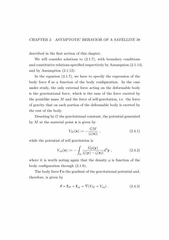
In the equation (2.1.7), we have to specify the expression of thebody force f as a function of the body configuration. In the caseunder study, the only external force acting on the deformable bodyis the gravitational force, which is the sum of the force exerted bythe pointlike mass M and the force of self-gravitation, i.e. the forceof gravity that on each portion of the deformable body is exerted bythe rest of the body.
Denoting by G the gravitational constant, the potential generatedby M at the material point x is given by
VM (x) := − GM
|ζ(x)| , (2.4.1)
while the potential of self gravitation is
Vsg(x) := −∫
Ω
Gρ(y)|ζ(y)− ζ(x)|d
3y , (2.4.2)
where it is worth noting again that the density ρ is function of thebody configuration through (2.1.8).
The body force f is the gradient of the gravitational potential and,therefore, is given by
f = fM + fsg = ∇(VM + Vsg) . (2.4.3)

CHAPTER 2. ASYMPTOTIC BEHAVIOR OF A SATELLITE 40
Since the main result that we will obtain in the next section is aconsequence of LaSalle’s principle, it is crucial to give a characteri-zation of those solutions to (2.1.7) such that there is no dissipationof energy, i.e. d
dtE(u, u) = 0 along the solution.
What we prove in this section is that the non-dissipating condi-tion can be fulfilled only if the pointlike mass M is immobile in thereference frame of the extended body.
The heuristic idea behind the result stated in this section is thefollowing: if there is no dissipation, then it means that the deforma-tion of the body does not change in time, i.e. the motion is rigid-like.Now, fix a reference frame co-moving with the extended body. Con-sider the forces acting on the body: in the body frame, the stresstensor is constant in time, and the self-gravitation force is also con-stant, since the motion is rigid-like. The fact that the motion isrigid-like suggests that also the gravitational force due to the bodyM should not vary in time (in the body frame), otherwise there wouldbe some change in the deformation. Of course, this is not obviousand it is what one really has to check.
Theorem 2.4.1. Let u(t) be a solution to (2.1.7), with constitutiverelations as in Assumption 1 and body force given by (2.4.3), suchthat
d
dtE(u, u) = 0 . (2.4.4)
Then, in a reference frame co-moving with the extended body, theposition of the pointlike mass M is constant in time.

CHAPTER 2. ASYMPTOTIC BEHAVIOR OF A SATELLITE 41
Proof. First of all, we remark that, due to Assumption 2, item (ii),the relation (2.4.4) is equivalent to requiring that ε = 0, i.e. at eachmaterial point the strain tensor is constant in time. Note that, dueto Assumption 1, this implies that also the stress tensor σ is constantin time at each material point. Since the strain tensor is constantat each point, then the body moves in space like a rigid body. Inorder to clarify this point, we observe that, if ε = 0, then the timederivative of the tensor of infinitesimal rotation ω must be the samefor all points of the deformable body. To prove this, fix a pointx0 ∈ Ω. Then we prove that
ω(x) = ω(x0)
for all x ∈ Ω. In fact, let γ be a path connecting x0 to x in Ω.Then, the value of ω(x) can be reconstructed from ω(x0) throughthe integration of a suitable first order differential form on the pathγ:
2ωij(x) = ∂ui∂xj
(x)− ∂uj∂xi
(x) = (2.4.5)
= 2ωij(x0) +∫γ
3∑l=1
∂2ui∂xj∂xl
dxl −∫γ
3∑l=1
∂2uj∂xi∂xl
dxl .
Through the definition of the strain tensor, we have
∂ui∂xl
= 2εil −∂ul∂xi
. (2.4.6)

CHAPTER 2. ASYMPTOTIC BEHAVIOR OF A SATELLITE 42
Differentiating with respect to xj , we find:
∂2ui∂xj∂xl
= 2∂εil∂xj− ∂2ul∂xj∂xi
. (2.4.7)
Exploiting (2.4.7), we can rewrite (2.4.5) as
2ωij(x) = 2ωij(x0) +∫γ
3∑l=1
(2∂εil∂xj− ∂2ul∂xj∂xi
)dxl +
−∫γ
3∑l=1
(2∂εjl∂xi− ∂2ul∂xi∂xj
)dxl =
= 2ωij(x0) + 2∫γ
3∑l=1
(∂εil∂xj− ∂εjl∂xi
)dxl . (2.4.8)
Now, differentiating with respect to time and exploiting ε = 0, wehave
ωij(x) = ωij(x0) . (2.4.9)
The condition of rigid motion may be expressed by saying that forall times there exists a vector ν (function of time, but independent ofthe material point), which is the angular velocity of the body, suchthat, for any fixed x0 ∈ Ω, the equation
ζ(x)− ζ(x0) = ν ∧ [ζ(x)− ζ(x0)] (2.4.10)
holds for all x ∈ Ω. Differentiating with respect to time, we obtain
ζ(x)− ζ(x0) = ν ∧[ζ(x)− ζ(x0)
]+ ν ∧ [ζ(x)− ζ(x0)] . (2.4.11)

CHAPTER 2. ASYMPTOTIC BEHAVIOR OF A SATELLITE 43
Substituting (2.4.10) in (2.4.11), we get
ζ(x)− ζ(x0) = ν∧ν ∧ [ζ(x)− ζ(x0)]+ν∧[ζ(x)− ζ(x0)] . (2.4.12)
Now, let us work in the physical space instead of the materialone, denoting by ξ the Cartesian coordinates of the physical space.Denoting by a and a0, respectively, the accelerations at ξ and ξ0, theequation (2.4.12) above can be rewritten as
ξ − ξ0 = ν ∧ [ν ∧ (ξ − ξ0))] + ν ∧ (ξ − ξ0)) . (2.4.13)
This equation holds for all times. In particular, (2.4.13) implies that,for all times, the acceleration field is a linear function of the positionin the physical space.
If we look back at the structure of equation (2.1.7), we notice thatit is nothing else but the local form of Newton’s law: the accelerationat each point (note that a = u) equals the total force (which is thesum of body forces and internal stresses) per unit mass acting onthe same point. But this observation, together with (2.4.13), impliesthat for each fixed time, the total force per unit mass is a linearfunction of the position inside the body. In particular, this impliesthat the second (and higher order) differential with respect to thespace variables of the total force per unit mass is identically zero.
In other words, for any fixed time, we have that
d2
dξ2
(fi + 1
ρ
∂
∂xjσij
)= 0 , (2.4.14)
CHAPTER 2. ASYMPTOTIC BEHAVIOR OF A SATELLITE 44
where the terms fi and ∂∂xj
σij must be thought of as functions ofthe ξ variables. This is a geometric property of the field of forcesacting upon the extended body, which is verified for all times andis independent of the reference frame. In fact a change of referenceframe is not a generic change of coordinates: changing the referenceframe corresponds to making a linear change of coordinates and theproperty of linearity of a vector field is conserved when applying alinear change of coordinates.
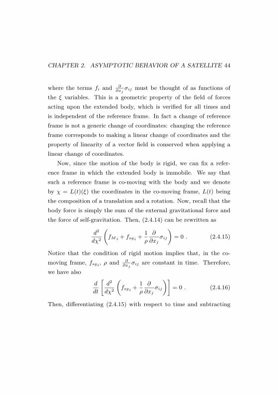
Now, since the motion of the body is rigid, we can fix a refer-ence frame in which the extended body is immobile. We say thatsuch a reference frame is co-moving with the body and we denoteby χ = L(t)(ξ) the coordinates in the co-moving frame, L(t) beingthe composition of a translation and a rotation. Now, recall that thebody force is simply the sum of the external gravitational force andthe force of self-gravitation. Then, (2.4.14) can be rewritten as
d2
dχ2
(fMi + fsgi + 1
ρ
∂
∂xjσij
)= 0 . (2.4.15)
Notice that the condition of rigid motion implies that, in the co-moving frame, fsgi, ρ and ∂
∂xjσij are constant in time. Therefore,
we have also
d
dt
[d2
dχ2
(fsgi + 1
ρ
∂
∂xjσij
)]= 0 . (2.4.16)
Then, differentiating (2.4.15) with respect to time and subtracting
CHAPTER 2. ASYMPTOTIC BEHAVIOR OF A SATELLITE 45
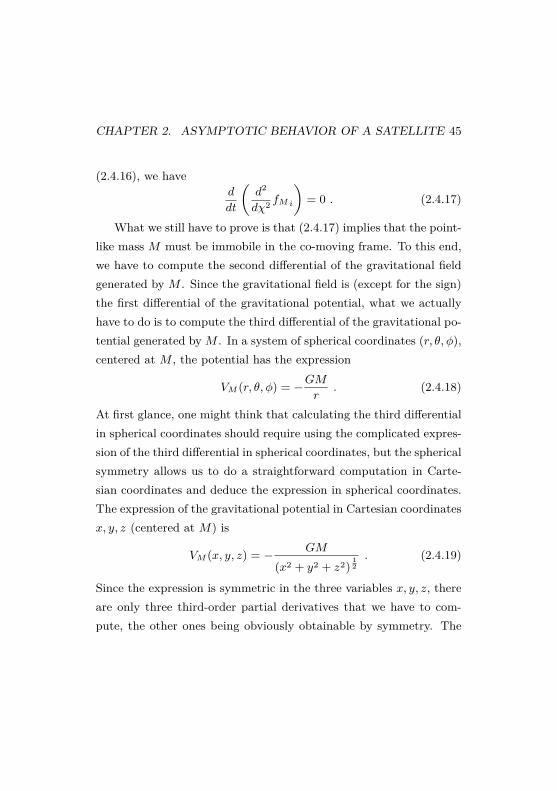
(2.4.16), we haved
dt
(d2
dχ2 fMi
)= 0 . (2.4.17)
What we still have to prove is that (2.4.17) implies that the point-like mass M must be immobile in the co-moving frame. To this end,we have to compute the second differential of the gravitational fieldgenerated by M . Since the gravitational field is (except for the sign)the first differential of the gravitational potential, what we actuallyhave to do is to compute the third differential of the gravitational po-tential generated byM . In a system of spherical coordinates (r, θ, φ),centered at M , the potential has the expression
VM (r, θ, φ) = −GMr
. (2.4.18)
At first glance, one might think that calculating the third differentialin spherical coordinates should require using the complicated expres-sion of the third differential in spherical coordinates, but the sphericalsymmetry allows us to do a straightforward computation in Carte-sian coordinates and deduce the expression in spherical coordinates.The expression of the gravitational potential in Cartesian coordinatesx, y, z (centered at M) is
VM (x, y, z) = − GM
(x2 + y2 + z2)12. (2.4.19)
Since the expression is symmetric in the three variables x, y, z, thereare only three third-order partial derivatives that we have to com-pute, the other ones being obviously obtainable by symmetry. The

CHAPTER 2. ASYMPTOTIC BEHAVIOR OF A SATELLITE 46
computations yield
∂3VM∂x3 (x, y, z) = 3GMx(2x2 − 3y2 − 3z2)
(x2 + y2 + z2)72
(2.4.20)
∂3VM∂x2∂y
(x, y, z) = 3GMy(4x2 − y2 − z2)(x2 + y2 + z2)
72
(2.4.21)
∂3VM∂x∂y∂z
(x, y, z) = 15GMxyz
(x2 + y2 + z2)72. (2.4.22)
The next step is simply to evaluate these partial derivatives in a pointof the form (x0, 0, 0), so that x represents the radial direction and y, zrepresent any direction orthogonal to the radial one. We find
∂3VM∂x3 (x0, 0, 0) = 6GM
x04 (2.4.23)
∂3VM∂x∂y2 (x0, 0, 0) = ∂3VM
∂x∂z2 (x0, 0, 0) = −3GMx04 , (2.4.24)
all the other partial derivatives being zero, when evaluated at (x0, 0, 0).By the spherical symmetry of the potential, we deduce the generalexpressions in spherical coordinates
∂3VM∂r3 (r, θ, φ) = 6GM
r4 (2.4.25)
∂3VM∂r∂θ2 (r, θ, φ) = ∂3VM
∂r∂φ2 (r, θ, φ) = −3GMr4 (2.4.26)
∂3VM∂θ3 = ∂3VM
∂φ3 = ∂3VM∂r2∂θ
= ∂3VM∂r2∂φ
= 0 (2.4.27)

CHAPTER 2. ASYMPTOTIC BEHAVIOR OF A SATELLITE 47
∂3VM∂φ∂θ2 = ∂3VM
∂φ2∂θ= ∂3VM∂r∂θ∂φ
= 0 . (2.4.28)
We have said that the third differential of the potential VM mustbe constant in time at any point of the extended body, in the co-moving frame. Actually, it will be enough to impose the conditionthat along the motion the third differential of the potential is con-served at a fixed point in the extended body, which is the imagethrough the configuration map ζ(t) of a fixed material point x0. Now,let us consider a reference frame with origin at the point ζ(x0) andaxes oriented along the r, θ and φ directions. A priori such a refer-ence frame is not necessarily co-moving with the extended body. Thecomponents of a vector X in this reference frame will be denoted byXr, Xθ, Xφ.
The third-order differential of VM is a trilinear form, which hasan associated cubic form
C(X) := d3VM (ζ(x0))(X,X,X) = (2.4.29)
= 3GM|ζ(x0)|4
[Xr(2Xr2 − 3Xθ2 − 3Xφ2)]
Now, the conservation of the third differential of VM implies that, inthe co-moving frame, also the cubic form C must be constant, i.e.given any vector Xc(t) co-moving with the extended body,
d
dtC[Xc(t)] = 0 (2.4.30)
must hold. This obviously implies that also the set of zeros of thecubic form must be conserved in the co-moving frame. Now, the set

CHAPTER 2. ASYMPTOTIC BEHAVIOR OF A SATELLITE 48
of zeros of C is
Z =X ∈ R3|Xr
(2Xr2 − 3Xθ2 − 3Xφ2) = 0
,
which is the union of a plane orthogonal to the radial direction and acircular cone, whose axis is oriented along the radial direction. Thisargument shows that the radial direction (i.e. the direction of theline joining the pointlike massM with ζ(x0)) must be fixed in the co-moving frame. In other words, we can choose a co-moving frame withorigin at ζ(x0) in such a way that one of the axes is always orientedalong the radial direction: we choose this axis to be oriented from M
to ζ(x0). We denote the unit vector associated to this axis with er,so that the unit vectors of the co-moving frame will be (er, ey, ez),ey and ez being chosen arbitrarily. In this way, the coordinates of Min the co-moving frame are (−|ζ(x0)|, 0, 0).
Now, observe that
C(er) = 6GM|ζ(x0)|4 . (2.4.31)
This, together with (2.4.30), implies that |ζ(x0)| must be constant intime. Finally, this implies that the pointlike mass M is immobile inthe co-moving frame, which ends the proof of the theorem.
In accordance with LaSalle’s principle, we define the non-dissipatingmanifold and the largest invariant set contained in it.
Definition 2.4.2. The non-dissipating manifold is
ND :=
(u, v) ∈ X| ddtE(u, v) = 0
.

CHAPTER 2. ASYMPTOTIC BEHAVIOR OF A SATELLITE 49
Definition 2.4.3. We define NDinv to be the largest invariant setcontained in ND.
We remark that, if the pointlike massM occupies a fixed positionin the co-moving frame, then the extended body shows always thesame face to M , which is exactly what happens when the satellite isin synchronous resonance.
Then, the consequence of Theorem 2.4.1 is that NDinv is a unionof orbits of constant radius such that the extended body moves rigidlyalong the orbit in synchronous resonance. In non-degenerate cases,NDinv is expected to be made up of a single orbit. In the nextchapter, we will provide an example of both non-degenerate and de-generate cases.
2.5 The “three outcomes” theorem
In this section we exploit LaSalle’s principle in order to prove what wecall the theorem of the “three outcomes”. The meaning of the theoremis that, in a system made up of an elastic satellite with friction anda pointlike planet whose space coordinates are fixed, there are onlythree admissible outcomes for the final behavior of the satellite:
(i) the satellite is expelled to infinity;
(ii) the satellite falls on the planet;
(iii) the satellite is captured in synchronous resonance.

CHAPTER 2. ASYMPTOTIC BEHAVIOR OF A SATELLITE 50
For the discussion of the present section, it is convenient to isolatethe motion of the center of mass of the satellite from the rest of theinformation related to the body configuration. Therefore, we definethe center of mass
X = 1m
∫Ωζ(x)ρ(x)d3x (2.5.1)
and the “centered configuration”
v(x) := ζ(x)−X . (2.5.2)
of course, knowing X and the centered configuration v(x) is equiva-lent to knowing the whole configuration ζ(x). Therefore, the Cauchyproblem (2.2.3) can be reformulated in terms of X and v. In thisway we are decomposing the phase space as
(R3 \ 0
)× R3 × Y ,(
R3 \ 0)× R3 being the space where position and velocity of X
live and Y being defined as the phase space related to the centeredconfiguration v.
In order to prove our result, we need some definitions and tech-nical hypotheses. First of all, we need to deal with the case of theimpact between the satellite and the planet M . We remark that theproblem has a singularity, in the sense that the equations of motionare not defined if the position a point of the satellite coincides withthe position of the planet M , i.e. if there exists a point x0 ∈ Ω suchthat ζ(x0) = 0.

CHAPTER 2. ASYMPTOTIC BEHAVIOR OF A SATELLITE 51
Definition 2.5.1. A solution to the Cauchy problem (2.2.3) (withany initial datum) is said to be impacting the planet (in the future)Mif for all ε > 0 there exists a time t > 0 such that dist(ζ(Ω, t), 0) < ε.
Then we make the following assumption about the existence timeof solutions to (2.2.3).
Assumption 3. The existence time of a solution to (2.2.3) is infinite(in the future) if and only if the solution is not impacting the planet.
We observe that this assumption implies that, if an impact isthere, it takes a finite amount of time for the impact to occur. More-over, it rules out the possibility of the occurrence of any sort ofblow up which might correspond to some fracture, disintegration,or, generally speaking, singularity formation in the configuration ofthe satellite.
Then the following proposition is immediate.
Proposition 2.5.2. A solution is not impacting the planet if andonly if there exists δ > 0 such that dist(ζ(Ω, t), 0) ≥ δ for all timest > 0.
The next assumption is a rather technical one: in fact, LaSalle’sinvariance principle applies to orbits contained in a compact set. Atthe same time, bounded subsets of infinite-dimensional spaces are notnecessarily pre-compact. In our case, what we need to assume is ausual fact in viscous-type equations. A typical effect of viscosity is thedamping of high-frequency modes, which leads to pre-compactness

CHAPTER 2. ASYMPTOTIC BEHAVIOR OF A SATELLITE 52
properties of orbits in the future. Such properties are usually de-duced by performing estimates which make use of the explicit formof the equations of motion. In our case, since we are dealing withquite a general setting, and we have no explicit expressions for theconstitutive equations, we assume the following property.
Assumption 4. For any initial datum, the solution to (2.2.3) issuch that the corresponding future orbit (v(t), v(t))|t > 0 ⊂ Y ofthe centered configuration is pre-compact.
Finally, we assume the following property about the energy of thesatellite.
Assumption 5. The functional
F (u) := Esg(u) + Eel(u)
is bounded below.
We remark that the above assumption is satisfied if, in partic-ular, the satellite has an equilibrium configuration under the effectof elastic stresses and self-gravitation which globally minimizes theassociated energy.
We are now ready to state the main theorem.
Theorem 2.5.3 (Theorem of the three outcomes). Let Assumptions1, 2, 3, 4 and 5 be satisfied. Then, for a solution to (2.2.3), one ofthe following three (future) scenarios must occur:

CHAPTER 2. ASYMPTOTIC BEHAVIOR OF A SATELLITE 53
(i) the trajectory of the center of mass X is unbounded;
(ii) the solution impacts the planet;
(iii) the solution is asymptotic to the non-dissipating invariant man-ifold NDinv.
Proof. The proof of the theorem is actually a simple application ofLaSalle’s invariance principle. We are going to prove that any futureorbit which does not satisfy either (i) or (ii) must necessarily satisfy(iii).
Let therefore γ be the orbit corresponding to the solution to(2.2.3), for some given initial data. Assume that γ does not sat-isfy either (i) or (ii). Then, by Proposition 2.5.2, we can concludethat the future trajectory ofX is bounded above and below, i.e. thereexist k,K > 0 such that k ≤ |X| ≤ K for all times.
In order to conclude that the velocity X is bounded, we first lookat the form of the energy functional
E(u, u) = Ekin(u, u) + Eg(u) + Esg(u) + Eel(u) .
Observe that the sum Esg(u)+Eel(u) is bounded below, by Assump-tion 5. Furthermore, Eg(u) is bounded below because, by Proposition2.5.2, there exists δ such that dist(ζ(Ω), 0) ≥ δ for all times. Then,by the non-increasing energy inequality (2.2.4), we can conclude thatthe kinetic energy Ekin(u, u) is bounded above in the future. Then,by König’s second theorem, the total kinetic energy must be greater

CHAPTER 2. ASYMPTOTIC BEHAVIOR OF A SATELLITE 54
or equal to the kinetic energy of the center of mass of the satel-lite. Therefore, the kinetic energy of the center of mass of the satel-lite must be bounded above in the future, which implies that X isbounded above in the future.
Then, since the future orbit of (X, X) is contained in a com-pact subset of
(R3 \ 0
)× R3 and the future orbit of the centered
configuration (v, v) is pre-compact, then the future orbit of (u, u)is pre-compact in X. Therefore, we can apply LaSalle’s invarianceprinciple, which states that the solution is asymptotic to the non-dissipating invariant manifold NDinv, which concludes the proof ofthe theorem.
2.5.1 Comments about the meaning of the theorem ofthe three outcomes
In order to understand the content of the theorem of the three out-comes, we should first remark what it does not say. First of all, thetheorem in itself says nothing about the stability of the synchronousresonance. At the same time, if one is able to prove the orbital sta-bility of the synchronous resonance (which, apart from the matter ofgiving a rigorous proof, is something which is strongly expected tobe true), then the local asymptotic stability is a trivial consequenceof the theorem.
Some comment is needed about the meaning of the three out-

CHAPTER 2. ASYMPTOTIC BEHAVIOR OF A SATELLITE 55
comes.Let us first consider the outcome (i), i.e. the case of unbounded
orbit. The fact that the trajectory of the center of mass of the satel-lite is unbounded does not necessarily mean that it tends to infinity.In fact, one cannot a priori rule out the possibility that, along withan unbounded trajectory of the center of mass, there exist R > 0and tn → +∞ such that |X(tn)| < R. Anyway, if one can prove theorbital stability of the synchronous resonance, then a simple appli-cation of 2.3.6 proves that an unbounded trajectory of the center ofmass must actually tend to infinity. In fact, under the assumption oforbital stability, one proves that, if there were R > 0 and tn → +∞such that |X(tn)| < R, then the orbit should be asymptotic to thesynchronous resonance, which cannot be the case if the orbit is un-bounded.
The outcome (ii) has the clear meaning of a planet-satellite colli-sion and does not need any further explanation.
The outcome (iii) is the one we informally refer to as asymptot-ically being trapped into the synchronous resonance, since the char-acterization explained in Section 2.4 shows that the only possiblenon-dissipating behavior of the satellite is that of synchronous reso-nance, in the sense that the satellite always shows the same face tothe planet, revolving about it at a fixed distance. Actually, in theleast degenerate case, where the non-dissipating invariant manifoldNDinv is made up of only one orbit, the outcome (iii) clearly implies

CHAPTER 2. ASYMPTOTIC BEHAVIOR OF A SATELLITE 56
asymptoticity to such an orbit; however, in presence of very degen-erate non-dissipating invariant manifolds, the outcome (iii) could apriori not result in asymptoticity to a synchronous resonant orbit.In order to perform some more accurate analysis of the manifoldNDinv, one should add some assumptions about the structure of thesatellite. However, in the next chapter we analyze, in the planarapproximation (which we will specify in the next chapter), the tworelevant cases of a triaxial satellite and of a satellite with sphericalsymmetry. In the triaxial case, the non-dissipating invariant manifoldturns out to be completely non-degenerate; in the spherically sym-metric case, the non-dissipating invariant manifold turns out to be aslightly degenerate one, in a sense that we will discuss later. In sucha slightly degenerate situation, the outcome (iii) can still be referredto as asymptotically approaching the synchronous resonance.
A remarkable fact is that, anyway, the discussion of the presentchapter excludes the possibility that other periodic orbits exist, dif-ferent from the synchronous resonant ones. This may seem quitesurprising, since, for instance, some celestial bodies are known to betrapped in spin-orbit resonances different from the synchronous one(think, for example, of the 3:2 of Mercury, seen as a satellite of theSun). At the same time, from our point of view, it is natural to thinkthat any periodic orbit different from the synchronous resonant onewould cause some periodic deformation of the satellite. Such a peri-odic deformation would, in turn, produce some periodic dissipation.

CHAPTER 2. ASYMPTOTIC BEHAVIOR OF A SATELLITE 57
But one cannot continue dissipating periodically the same amountof energy for an infinite time, since this would lead the energy to−∞, implying that a collision is going to occur. Our interpretationis that situations like the 3:2 resonance of Mercury are very likely tobe metastable, and it would be very interesting to investigate furtherin this direction. For instance, one could try to give an estimate ofthe time of such a metastability: it would not be so surprising if sucha time were of the same order of magnitude as the estimated lifespanof the Solar system.


Chapter 3
Orbital stability
In this chapter, as we did in the previous one, we will deal with adynamical system made up of a a pointlike mass M (the “planet”),whose space coordinates are fixed at the origin of the Euclidean spaceR3, and an elastic body (the “satellite”) with internal friction, subjectto the force of gravity exerted by M .
Our aim here is to prove the orbital stability of the synchronousresonance. We will give the proof of the stability in two cases:
(i) triaxial satellite;
(ii) satellite with spherical symmetry.
The proof of the orbital stability will be done under some approx-imations. Namely, we will make the planar approximation (which we
59

CHAPTER 3. ORBITAL STABILITY 60
will explain later) and we will truncate the expansion of the gravi-tational potential at the quadrupole terms, neglecting higher ordereffects.
In both cases, we make the convenient assumption that the elas-ticity moduli of the satellite are very large.
Before making some kinematic considerations, let us say what wemean by “triaxial satellite”. To this end, we have to recall some basicfacts about moments and axes of inertia.
We first need to recall what the matrix of inertia is. In principle,one may evaluate the matrix of inertia of an extended body withrespect to any point in space; however, we will always refer to thematrix of inertia evaluated with respect to the center of mass.
Let B be an extended body which occupies a volume V in thethree-dimensional Euclidean space. Fix a Cartesian frame of refer-ence (x, y, z), with origin in the center of mass of B and let ρ(x, y, z)be the density function of B. Then the matrix of inertia of B is asymmetric matrix I11 I12 I13
I12 I22 I23
I13 I23 I33
where
I11 =∫ ∫ ∫
V
ρ(x, y, z)(y2 + z2)dxdydz (3.0.1)
I22 =∫ ∫ ∫
V
ρ(x, y, z)(x2 + z2)dxdydz (3.0.2)

CHAPTER 3. ORBITAL STABILITY 61
I33 =∫ ∫ ∫
V
ρ(x, y, z)(x2 + y2)dxdydz (3.0.3)
I12 = −∫ ∫ ∫
V
xyρ(x, y, z)dxdydz (3.0.4)
I13 = −∫ ∫ ∫
V
xzρ(x, y, z)dxdydz (3.0.5)
I23 = −∫ ∫ ∫
V
yzρ(x, y, z)dxdydz . (3.0.6)
Since the matrix of inertia is a real symmetric matrix, it has realeigenvalues. The eigenvalues of the matrix of inertia are the principalmoments of inertia of B. If the three eigenvalues are distinct, thenthe directions of the three associated eigenvectors are well definedand individuate the principal axes of inertia of B.
As we will show later, the principal moments and axes of inertiaare very relevant objects in the study of our problem. On the oneside, the kinematic study of extended bodies rotating in space in-volves the concept of moment of inertia. On the other side, which ismore specific to our problem, if one expands in multipoles the grav-itational interaction of an extended body with a pointlike mass andneglects terms beyond quadrupole, the only relevant parameters ofthe extended body (apart from its mass and the position of its centerof mass) are found to be the principal moments of inertia and thedirections of the principal axes of inertia.
A rigid body is called triaxial if its three moments of inertia aredistinct. In our framework, we deal with a body (the satellite) which

CHAPTER 3. ORBITAL STABILITY 62
is not rigid. When we talk about triaxiality of the satellite, we meanthat the satellite is triaxial when it reaches its configuration of equilib-rium between the elastic and self-gravitating forces. In other words,the satellite is triaxial if the three eigenvalues of the matrix of inertiaare distinct when the satellite is in such an equilibrium configuration.
In the triaxial case, the orbital stability of the synchronous res-onance is a consequence of the orbital stability for a triaxial rigidbody, the deformable case being a small perturbation of the rigidone.
In the spherically symmetric case, instead, there is no orbitalstability of the synchronous resonance for a rigid body, and such astability appears as a consequence of the tidal deformation of thesatellite.
For this reason, the proof of orbital stability will be quite straight-forward in the triaxial case, while it will require a careful and rathertechnical kinematic analysis in the spherically symmetric case.
3.1 General setting and global rotations
Let us now recall some notation we have already used in the pre-vious chapter, only to fix ideas. Let Ω be the material space andlet ζ : Ω → R3 be the body. In this chapter we assume that, inthe reference configuration ζ0(x) = x, elastic forces and forces ofself-gravitation are in equilibrium in the satellite. As in the previ-ous chapter, we denote by ρ0 : Ω → R the density function in the

CHAPTER 3. ORBITAL STABILITY 63
reference configuration and by ρ : Ω → R the density function in ageneric configuration ζ, which is related to ρ0 by (2.1.8). Withoutloss of generality, we assume that the center of mass in the referenceconfiguration is at the origin, i.e.∫
Ωxρ0(x)d3x = 0 . (3.1.1)
The map ζ describes both the deformation of the body and itsposition and rotation in space, so it is natural to try to decompose ζinto a rigid translation, a rigid rotation and an internal deformation.As in the previous chapter, we define the center of mass of the bodyby
X = 1m
∫Ωζ(x)ρ(x)d3x , (3.1.2)
and decompose the configuration vector field ζ as
ζ(x) = X + v(x) , (3.1.3)
where v is such that ∫Ωv(x)ρ(x)d3x = 0 . (3.1.4)
Denote by C the space of the v’s such that (3.1.4) holds.
Remark 3.1.1. The space C is an infinite dimensional functionspace, so in order to discuss dynamics one should introduce a suitablenorm in it, prove an existence and uniqueness theorem for the solu-tions to the Cauchy problem and, in order to use energy conservation

CHAPTER 3. ORBITAL STABILITY 64
(or dissipation) to prove dynamical properties, one should also provethat dynamics is well posed in the energy space, which is in generalunknown [26].
Here, we do not want to enter such a kind of mathematical prob-lems, so we will simply assume existence and uniqueness for the so-lutions to the Cauchy problem and well-posedness of the dynamicsin the energy space.
Now the body configuration is uniquely parameterized throughthe position X of the center of mass and the function v ∈ C. Thereference configuration corresponds to X0 = 0, v0(x) = x.
Then we would like to factor out rotations in a way similar totranslations, however this requires a careful discussion. The point isthat it is clear what it means to rotate a body, but it is not clear howto say that a deformation does not rotate the body: as we will see,this is not a well defined concept.
To understand this point, we recall the standard analysis of thelocal deformation in linear elasticity theory, as explained in the previ-ous chapter. Fix a point x0 ∈ Ω. Then, the displacement vector fieldis defined by u(x) := ζ(x)− x. The gradient ∇u(x0) is decomposedas the sum of its symmetric part ε and its skew-symmetric part ω.Then, at the point x0, the local deformation is described by the straintensor ε, while the skew-symmetric part of the gradient ω describesthe local rotation. Thus, at a local level, the separation betweendeformation and rotation is well-defined and completely standard.

CHAPTER 3. ORBITAL STABILITY 65
On the other hand, when considering the global configuration, thesituation is more complicated, because it is not trivial at all to answerthe following question. Let the configuration ζ be assigned. Is thecorresponding displacement vector field u a “pure deformation”, in thesense that it does not “globally rotate the body”, or is it given by thecomposition of a rotation of the body with some “pure deformation”?
The answer to this question is easy if one considers only affinedeformations, i.e. if one allows only displacements whose gradient isspatially constant. In fact, in this case, the rotation is simply de-scribed by the skew-symmetric part of the gradient of the displace-ment (evaluated at any point, since it is constant).
Nevertheless, if one wants to deal with general displacement fields,no obvious answer can be given to the previous question. One couldtry to give some reasonable definitions of what a “pure deformation”is. For instance, we could fix x0 ∈ Ω and say that u is a “pure de-formation” if the displacement, locally at x0, does not contain anyrotation, i.e. ∇u(x0) is symmetric. Anyway, this seems quite ar-bitrary; moreover, different choices of x0 would result in differentdefinitions of “pure deformation”.
In order to make it independent of the particular choice of a point,one could try to give the definition of “pure deformation” through anintegral condition. This is done, for instance, in [31, 35], where sucha definition (in the case of an incompressible homogeneous body) is
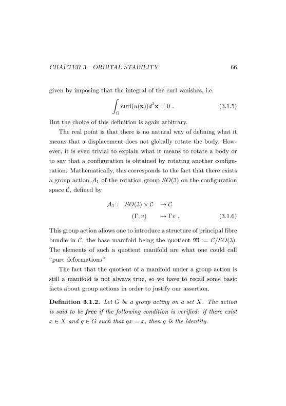
CHAPTER 3. ORBITAL STABILITY 66
given by imposing that the integral of the curl vanishes, i.e.∫Ω
curl(u(x))d3x = 0 . (3.1.5)
But the choice of this definition is again arbitrary.The real point is that there is no natural way of defining what it
means that a displacement does not globally rotate the body. How-ever, it is even trivial to explain what it means to rotate a body orto say that a configuration is obtained by rotating another configu-ration. Mathematically, this corresponds to the fact that there existsa group action A1 of the rotation group SO(3) on the configurationspace C, defined by
A1 : SO(3)× C → C
(Γ, v) 7→ Γv . (3.1.6)
This group action allows one to introduce a structure of principal fibrebundle in C, the base manifold being the quotient M := C/SO(3).The elements of such a quotient manifold are what one could call“pure deformations”.
The fact that the quotient of a manifold under a group action isstill a manifold is not always true, so we have to recall some basicfacts about group actions in order to justify our assertion.
Definition 3.1.2. Let G be a group acting on a set X. The actionis said to be free if the following condition is verified: if there existx ∈ X and g ∈ G such that gx = x, then g is the identity.

CHAPTER 3. ORBITAL STABILITY 67
Definition 3.1.3. The action of a topological group G on a topolog-ical space X is said to be proper if the mapping
G×X → X ×X (g, x) 7→ (gx, x)
is proper, i.e., inverses of compact sets are compact.
Theorem 3.1.4. Let G be a topological group acting on a topologicalspace M . If G is compact, then the action is proper.
Theorem 3.1.5. If a Lie group G acts freely and properly on asmooth manifold, then the quotient M/G is a smooth manifold.
In our case, the fact that SO(3) is a compact group and that theaction A1 is obviously free implies that M is a manifold.
As usual in this geometric context, it is useful to introduce coordi-nates in which a point of C is represented by an element of SO(3) andan element of the base manifold. However a concrete representationof the elements of the quotient manifold can be obtained only locally,by introducing a local section of the bundle, namely by choosing asubmanifold S of C, transversal to the group orbit. Now it is clearthat there are infinitely many possible choices of the section of thebundle, which correspond to infinitely many admissible definitions of“pure deformations”. Nonetheless, the physics is independent of thechoice of the section S: a change in the choice of the section simplyresults in a change of coordinates. The fact that the section is onlylocal is not a problem, as long as only small deformations are allowed.

CHAPTER 3. ORBITAL STABILITY 68
Now, let A1(v0) be the orbit of the reference configuration underthe action of the group SO(3). Once the section has been chosen,it naturally induces a smooth one-to-one correspondence between aneighborhood of A1(v0) (obtained as the union of the orbits of thepoints of S under the group action A1) and SO(3)×S. Such a cor-respondence allows one to parameterize the space C of configurationsthrough an element of the group SO(3) and a point of the sectionS. In the context of classical mechanics, this is useful, since, dueto the isotropy of space, the Lagrangian of the body is going to beindependent from the element of SO(3) and will depend only on thevariable belonging to S.
We remark that the machinery we have just introduced describes ageneral fact, which is independent of all the assumptions we will makelater in the paper. We can summarize the result of our discussion inthe following theorem:
Theorem 3.1.6. There exist a neighborhood U ⊂ C of A1(v0) and aone-to-one smooth function f : SO(3)×S→ U with the property thatf(Γ, w) = A1(Γ)w. Therefore, Γ and w can be used as coordinateson the configuration space C.

CHAPTER 3. ORBITAL STABILITY 69
3.2 The matrix of inertia as a function of the con-figuration
Since the satellite is deformable, in our setting the matrix of inertiaof the satellite is not a fixed object, but it is a function of the bodyconfiguration. In a compact notation, the elements Iij3i,j=1 of theinertia matrix I are given by the following formula:
Iij = Iij(v) := ei ·∫
Ωv(x) ∧ (ej ∧ v(x))ρ(x)d3x . (3.2.1)
In the rest of the chapter we will always denote with the doublesubscript the elements Iij of the matrix of inertia, while the principalmoments of inertia (i.e., the eigenvalues of the matrix I) will bedenoted by I1, I2, I3. Again, we remark that the principal momentsof inertia are a function of the body configuration. The principalaxes of inertia are also functions of the body configuration and wewill denote them by u1, u2, u3.
3.3 Planar restriction
We are going to study the dynamics of the satellite in the specialcase when the motion of the center of mass of the satellite is planarand the spin axis of the body is orthogonal to the plane of the orbitand coincides with one of the principal axes of inertia of the body.For this reason, we will restrict to “planar motion of the center ofmass”, “planar deformations” and “planar rotations”. Precisely, we

CHAPTER 3. ORBITAL STABILITY 70
make the following assumptions. (Here and below we denote by e1,e2, e3 the vectors of the canonical base of R3.)
Assumption 6 (Planar motion of the center of mass). We assumethat X lies in the plane generated by e1 and e2.
Assumption 7 (Planar deformations). The configuration is suchthat e3 is an eigenvector of I. We label the principal axes of inertiaso that u3 = e3.
In other words, we are assuming the matrix of inertia of the satel-lite to be of the form
I(v) =
I11(v) I12(v) 0I12(v) I22(v) 0
0 0 I33(v)
, (3.3.1)
so that I3(v) ≡ I33(v).
Assumption 8 (Planar rotations). Γ is a rotation about the e3-axis,i.e. it has the form
Γ = Γ(α) :=
cosα − sinα 0sinα cosα 0
0 0 1
. (3.3.2)
3.4 The gravitational interaction
In this section we prove that, in the quadrupole approximation, thegravitational potential of the satellite, in the Newtonian field gener-ated by M , depends only on:

CHAPTER 3. ORBITAL STABILITY 71
(i) the mass of the satellite;
(ii) the position of the center of mass of the satellite;
(iii) the principal moments of inertia of the satellite;
(iv) the orientation of the principal axes of inertia of the satellite.
To start with, we fix some notation: (R,ψ) are the polar coordi-nates of the center of mass of the satellite in the plane of the orbit.We denote with γ the angle between the principal axis u1 and theline joining the planet to the center of mass of the satellite. Such aline is usually referred to as the line of centers. Then, we have thefollowing result.
Proposition 3.4.1. In the quadrupole approximation the gravita-tional potential energy of the body in the field generated by the massM is given by
Vg(X, I1, I2, I3, γ) := −GMm
R+GM
R3 [−I1+2I2−I3+3(I1−I2) cos2 γ] .(3.4.1)
Proof. Let (x1, x2, x3) be the Cartesian coordinates referred to thesystem with originX and axes u1u2u3. Then we introduce the spher-ical coordinates (r, ϑ, φ) of the generic point P in the satellite, defined

CHAPTER 3. ORBITAL STABILITY 72
by:
x1 = r cosϑ cosφ (3.4.2)
x2 = r sinϑ cosφ (3.4.3)
x3 = r sinφ . (3.4.4)
In this frame, the products of inertia Iij (i 6= j) vanish, i.e.∫ζ(Ω)
ρ(ξ)r2 cos2 φ cosϑ sinϑd3ξ = 0 (3.4.5)∫ζ(Ω)
ρ(ξ)r2 cosφ sinφ cosϑd3ξ = 0 (3.4.6)∫ζ(Ω)
ρ(ξ)r2 cosφ sinφ sinϑd3ξ = 0 , (3.4.7)
and the principal moments of inertia are given by
I1 = K2 +K3 (3.4.8)
I2 = K1 +K3 (3.4.9)
I3 = K1 +K2 , (3.4.10)
where
K1 = 12
∫ζ(Ω)
ρ(ξ)r2 cos2 φ cos2 ϑd3ξ (3.4.11)
K2 = 12
∫ζ(Ω)
ρ(ξ)r2 cos2 φ sin2 ϑd3ξ (3.4.12)
K3 = 12
∫ζ(Ω)
ρ(ξ)r2 sin2 φd3ξ . (3.4.13)

CHAPTER 3. ORBITAL STABILITY 73
The gravitational potential energy Vg is:
Vg = −∫ζ(Ω)
GMρ(ξ)|ξ| d3ξ = −
∫ζ(Ω)
GMρ(ξ)√R2 + r2 − 2Rr cos η
d3ξ ,
(3.4.14)where η is the angle between the line of centers and XP. Notice thatthe relation
cos η = cosφ cos (ϑ+ γ) (3.4.15)
holds. Let us recall now how the multipole expansion arises. We have1|ξ| = 1√
R2 + r2 − 2Rr cos η= 1R
1√1 +
(rR
)2 − 2(rR
)cos η
.
(3.4.16)In terms of the Legendre polynomials Pn(z), one has
1√1 + x2 − 2xz
=∑n≥0
xnPn(z) . (3.4.17)
In particular, we recall that
P0(z) = 1
P1(z) = z
P2(z) = 3z2 − 12 .
Taking the quadrupole approximation means to cut the sum at n = 2.We get
1|ξ| = 1
R
∑n≥0
(r
R
)nPn(cos η) ' 1
R
[1 + r
Rcos η +
(r
R
)2 3 cos2 η − 12
],
(3.4.18)

CHAPTER 3. ORBITAL STABILITY 74
so the potential energy becomes
Vg = −∫ζ(Ω)
GMρ(ξ)R
[1 + r
Rcos η +
(r
R
)2 3 cos2 η − 12
]d3ξ .
(3.4.19)Here, the first term equals −GMm
R; the second one vanishes because
X is the center of mass of the satellite; the third term, namely
Vt := −∫ζ(Ω)
GMρ(ξ)(3 cos2 η − 1)r2
2R3 d3ξ ,
gives what we call the “tidal” potential energy. A brief manipulationshows that
Vt = −GMR3
∫ζ(Ω)
ρ(ξ)(3 cos2 η − 1)r2
2 d3ξ =
= −GM2R3
∫ζ(Ω)
ρ(ξ)r2[3 cos2 φ cos2(ϑ+ γ)− 1]d3ξ =
= −3GMR3 (K1 cos2 γ +K2 sin2 γ) + GM
2R3
∫ζ(Ω)
ρ(ξ)r2d3ξ =
= −3GMR3 (K1 cos2 γ +K2 sin2 γ) +
+GM
2R3
∫ζ(Ω)
ρ(ξ)r2[sin2 φ+ cos2 φ(sin2 ϑ+ cos2 ϑ)]d3ξ =
= −3GMR3 (K1 cos2 γ +K2 sin2 γ) + GM
R3 (K1 +K2 +K3) =
= GM
R3 [−I1 + 2I2 − I3 + 3(I1 − I2) cos2 γ] . (3.4.20)

CHAPTER 3. ORBITAL STABILITY 75
The proposition we have proved in this section is the reason whyit is convenient to use the principal moments of inertia of the satelliteas Lagrangian coordinates in the study of our dynamical system.
3.5 Triaxial satellite
As we said above, triaxiality means that the three principal momentsof inertia of the satellite in its reference configuration v0 are all dis-tinct. Without loss of generality, we may assume that e1, e2 ande3 are the principal axes of inertia of the satellite in the referenceconfiguration.
Therefore, in the present section, we will assume that the follow-ing assumption is satisfied.
Assumption 9 (Triaxiality). The reference configuration v0 is suchthat I12(v0) = 0 and
I1(v0) = I11(v0) < I2(v0) = I22(v0) < I3(v0) = I33(v0) . (3.5.1)
Remark 3.5.1. The assumption on I3(v0) is actually useless, oncewe have done the planar restriction. However, this is the correctassumption that one should make in order to look for stability ofthe complete three-dimensional model, without the assumption of pla-narity. We leave the assumption in this form, in order to make phys-ically relevant the situation that we are studying. Anyway, in theplanar model, we could only assume I1(v0) 6= I2(v0), the sign of theinequality between I1 and I2 being determined by a choice of notation.
CHAPTER 3. ORBITAL STABILITY 76
We are now ready to prove the orbital stability of the synchronousresonance for a triaxial satellite. The scheme of the proof is thefollowing: we will first prove orbital stability for the conservativeLagrangian system that one obtains neglecting internal friction. Sucha proof involves conservation of energy. Then we observe that, ifone adds some extra dissipative force which makes energy a non-increasing function of time, then one still has orbital stability (in thefuture).
3.5.1 Lagrangian coordinates
By virtue of Assumption 8 and Theorem 3.1.6, we can use the fol-lowing set of Lagrangian coordinates:
• the polar coordinates (R,ψ) of the center of mass of the satel-lite;
• the angle χ := α−ψ, describing the rigid rotation of the satel-lite, measured with respect to the line of centers;
• a set of Lagrangian coordinates for w ∈ S.
We start with the idea of using the principal moments of inertia andan angle describing the orientation of the principal axes of inertia asLagrangian coordinates; however, there is the problem of singularityin the definition of the axes of inertia when two principal momentsof inertia have the same value. In the triaxial case, since we need not

CHAPTER 3. ORBITAL STABILITY 77
exploit any further symmetry (as, instead, we will have to do in thespherically symmetric case), we can get rid of the problem of such asingularity by simply using the matrix elements Iij(w) as coordinatesinstead of the eigenvalues and eigenvectors of the matrix of inertia.In order to do this, we need the following assumption.
Assumption 10. The functions
Iij : S→ R ,
(i, j) = (1, 1), (2, 2), (3, 3), (1, 2)
are independent in a neighborhood of v0.
Remark 3.5.2. The previous assumption is satisfied, for instance,if for any ij there exists a deformation which modifies Iij, leavingunaltered the other elements of the matrix I. The same assumptionwould not be satisfied if, for example, one added some additional con-straint, like the incompressibility constraint. In that case, one wouldhave to drop one degree of freedom.
If the assumption of independence is satisfied, then one can com-plete the set of Iij ’s to a system of coordinates on the local sectionS, which is expressed by the following proposition.
Proposition 3.5.3. There exist functions (z1, z2, . . .), with
zj : S→ R (j = 1, 2, . . .)
such that (I11, I22, I33, I12, z1, z2, . . .) is a set of smooth coordinateson S.
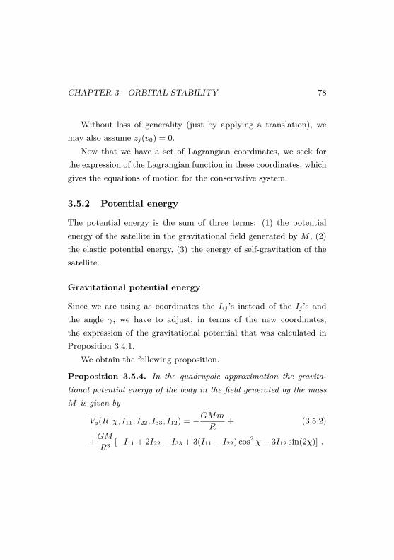
CHAPTER 3. ORBITAL STABILITY 78
Without loss of generality (just by applying a translation), wemay also assume zj(v0) = 0.
Now that we have a set of Lagrangian coordinates, we seek forthe expression of the Lagrangian function in these coordinates, whichgives the equations of motion for the conservative system.
3.5.2 Potential energy
The potential energy is the sum of three terms: (1) the potentialenergy of the satellite in the gravitational field generated by M , (2)the elastic potential energy, (3) the energy of self-gravitation of thesatellite.
Gravitational potential energy
Since we are using as coordinates the Iij ’s instead of the Ij ’s andthe angle γ, we have to adjust, in terms of the new coordinates,the expression of the gravitational potential that was calculated inProposition 3.4.1.
We obtain the following proposition.
Proposition 3.5.4. In the quadrupole approximation the gravita-tional potential energy of the body in the field generated by the massM is given by
Vg(R,χ, I11, I22, I33, I12) = −GMm
R+ (3.5.2)
+GM
R3 [−I11 + 2I22 − I33 + 3(I11 − I22) cos2 χ− 3I12 sin(2χ)] .

CHAPTER 3. ORBITAL STABILITY 79
Proof. We follow the proof of Proposition 3.4.1. Everything worksin the same way, except for the fact that we replace γ with χ andthat, correspondingly, in the frame co-rotating with the satellite, theproduct of inertia I12 does not vanish. Then we have the thesis.
Elastic and self-gravitational energy
In our model, the elastic and self-gravitational forces play, in somesense, the same role, since the combined action of both forces tendsto restore the reference configuration of the body and since theyare both independent of the rotation angle χ. Therefore, we willnot distinguish between the two corresponding potential energies.(With an abuse of language, we will refer to the sum of the elasticand self-gravitational potential energies simply as “elastic potentialenergy”.) We will also assume that the satellite has very large moduliof elasticity, which will correspond to having a very small parameterε. Using the notation I = (I11, I22, I33, I12), z = (z1, z2, . . .), wesummarize these facts in the following assumption.
Assumption 11. The elastic potential energy has the form
Ve(I, z) = 1εV0(I, z) , (3.5.3)
where ε is a small parameter Q and V0 has a nondegenerate minimumat (I, z) = (I0, 0), having set I0 := (I11(v0), I22(v0), I33(v0), I12(v0)).

CHAPTER 3. ORBITAL STABILITY 80
3.5.3 Kinetic energy
When evaluating the expression for the kinetic energy, it is convenientto express it in terms of the angle α = χ + ψ, which describes theactual speed of rotation of the satellite with respect to an inertialframe of reference. By König’s second Theorem, the kinetic energyT can be written as the sum of two terms: the former is the kineticenergy of the center of mass
Tcm = m
2 (R2 +R2ψ2) (3.5.4)
and the latter is the kinetic energy of the satellite with respect to itscenter of mass
Tr := Tr(α, I, z; I, z) . (3.5.5)
Remark 3.5.5. Tr is independent of α and due to the A1-invariance.
Since the kinetic energy with respect to the center of mass is aquadratic form in the corresponding velocities, we will use the nota-tion
Tr := 12
+∞∑i,k=1
aik(I, z)qiqk , (3.5.6)
where q = (α, I11, I22, I33, I12, z1, z2, . . .). Observe that the coeffi-cients aik(I, z) are such that the quadratic form is positive definiteon C.
Lemma 3.5.6. The coefficient a11(I, z) satisfies
a11(I, z) = I33 . (3.5.7)

CHAPTER 3. ORBITAL STABILITY 81
Proof. We havev(x) = Γ(α)w(x) . (3.5.8)
Taking the derivative with respect to time, we get
v(x) = dΓ(α)dt
w(x) + Γ(α)w(x) . (3.5.9)
Therefore,
Tr = 12
∫Ω
[v(x)]2ρ(x)d3x = 12
∫Ω
[Γ(−α)v(x)]2ρ(x)d3x =
= 12
∫Ω
[Γ(−α)dΓ(α)
dtw(x) + w(x)
]2
ρ(x)d3x =
= 12
∫Ω
[ω × w(x)]2 ρ(x)d3x + (3.5.10)
+∫
Ω〈ω × w(x), w(x)〉ρ(x)d3x + 1
2
∫Ω
[w(x)]2 ρ(x)d3x,
where ω is the angular velocity of the satellite, defined by
ω × (·) = [Γ(−α)][ ddt
Γ(α)](·)
. Under our assumptions, ω = αu3.As the vector field w(x) is independent of α, we observe that Tr
is the sum of three integrals, the first of which gives the term in α2,while the third one is a quadratic form in (I , z) and the second onegives mixed terms in α and in the other velocities.
Therefore, one gets
a11(I, z) =∫
Ωu3 × [x + u(x)]2 ρ(x)d3x , (3.5.11)

CHAPTER 3. ORBITAL STABILITY 82
and it can easily be seen that this expression equals the moment ofinertia related to the vertical axis, which concludes the proof of thelemma.
3.5.4 The reduced Lagrangian
The Lagrangian of the system is given by
L = T − V = Tcm + Tr − Vg − Ve , (3.5.12)
where each of the terms is given by the expressions calculated in theprevious sections. As a result, one gets
L = m
2(R2 +R2ψ2)+ Tr(χ+ ψ, I, z; I, z) + GMm
R+
+ GM
R3
[I11 − 2I22 + I33 + 3(I22 − I11) cos2 χ+ 3I12 sin(2χ)
]+
−Ve(I, z; ε) . (3.5.13)
Now, we observe that the Lagrangian does not depend on thecyclic coordinate ψ, so the total angular momentum
p := ∂L∂ψ
= mR2ψ + I33(χ+ ψ) + 2+∞∑k=2
a1k(I, z)qk , (3.5.14)
is a constant of motion. We can invert relation (3.5.14), to get theexpression of ψ as a function of the other variables:
ψ =p− I33χ− 2
∑+∞k=2 a1k(I, z)qk
mR2 + I33. (3.5.15)

CHAPTER 3. ORBITAL STABILITY 83
Then, we can drop one degree of freedom and study the reducedLagrangian
L∗ = L − ψ ∂L∂ψ
, (3.5.16)
where ψ must be thought of as a function of the other Lagrangiancoordinates and velocities. After some calculations, we get
L∗ = T2 + T1 − V , (3.5.17)
where
T2 = m
2 R2 + Tr(χ, I, z; I, z)−
[I33χ+ 2
∑+∞k=2 a1k(I, z)qk
]22(mR2 + I33)
T1 =p[I33χ+ 2
∑+∞k=2 a1k(I, z)qk
]mR2 + I33
V = p2
2(mR2 + I33) −GMm
R+
− GM
R3
[I11 − 2I22 + I33 + 3(I22 − I11) cos2 χ+ 3I12 sin(2χ)
]+
+ Ve(J, z; ε) .
The conservative system given by the corresponding Euler-Lagrangeequations has the conserved quantity
E := T2 + V =+∞∑k=1
yk∂L∗
∂yk− L∗ , (3.5.18)
wherey := (R,χ, I, z)

CHAPTER 3. ORBITAL STABILITY 84
and the strict minima of V are Lyapunov-stable equilibria of the re-duced system.
Let R0 be a nondegenerate minimum of the function
VG0(R) := −GMm
R+ p2
2(mR2 + I330) −GM
R3 (I330 + I220 − 2I110) ,
(3.5.19)where we have used the notation Iij0 := Iij(v0).
Then we have the following
Lemma 3.5.7. For any ε small enough, there exist R, χ, I, z, s.t.
(1) the point y := (R, χ, I, z) is a nondegenerate minimum of V .
(2) One has (|R−R0|, χ, |I − I0|, z) = O(ε).
(3) For all ψ ∈ S1, in the configuration of the unreduced systemcorresponding to (R, ψ, χ, I, z), the principal axis of inertia u1
is directed along the line of centers.
Remark 3.5.8. A fixed point in the reduced system corresponds toa situation of synchronous resonance on a circular orbit in the unre-duced system.
Proof. We look for a minimum of V in the domain |I − I0| ≤ Cε
for some fixed C. Observe that, if ε is small enough, |I − I0| ≤ Cε
implies both inequalities I1 < I2 < I3 (we remind that I12(v0) = 0)and I11 < I22 < I33, because of the triaxiality assumption. Moreover,if ε is small enough, also the inequality |I12| < I22 − I11 holds true.

CHAPTER 3. ORBITAL STABILITY 85
First consider V as a function of χ. Since |I12| < I22− I11, V hasa nondegenerate minimum at
χ = χ(I) := 12 arctan I12
I22 − I11. (3.5.20)
Comparison with (3.4.1) shows that the angle χ(I) corresponds toγ = 0 in (3.4.1); this will imply the point (3) of the lemma. Considernow V
∣∣χ=χ(I)
; as a function of R it has a nondegenerate minimumat some point R = R(I, z) fulfilling
|R(I, z)−R0| ≤ Cε .
Consider now the restriction V = V (I, z) of V to the manifold χ =χ(I), R = R(I, z); since
V (I, z) = 1εV0(I, z) +O(1) , (3.5.21)
such a function has a nondegenerate minimum close to zero.Then the thesis follows.
Corollary 3.5.9. The synchronous resonant circular orbit corre-sponding to y is orbitally stable for the Lagrangian system of equations
d
dt
∂L∂xk
= ∂L∂xk
, (k = 1, 2, . . .) (3.5.22)
where x = (R,ψ, χ, I, z).

CHAPTER 3. ORBITAL STABILITY 86
3.5.5 Dissipative dynamics
Now we modify the Euler-Lagrange equations of the previous sectionby introducing the effects of internal friction. To this end, we addterms −fk(x, x) to the Euler-Lagrange equations (3.5.22), so thatnow we are going to study the system of equations
d
dt
∂L∂xk− ∂L∂xk
= −fk(x, x) , (k = 1, 2, . . .) (3.5.23)
Moreover, since no dissipation acts on the orbital parameters,observe that the ψ-related term f2(x, x) must be identically zero.Furthermore, since the dissipative forces are only function of the timeevolution of the body configuration, all the fk’s must be independentof ψ and ψ. As a consequence, one is again allowed to pass to thereduced system
d
dt
∂L∗
∂yk− ∂L∗
∂yk= −fk(y, y) , (k = 1, 2, . . .) (3.5.24)
where the fk are obviously defined.Now, proceeding as for the proof of energy conservation, we get
the following lemma.
Lemma 3.5.10. In the system of differential equations (3.5.24), theLie derivative of the energy is given by
dE
dt= −
+∞∑k=1
ykfk(y, y) . (3.5.25)

CHAPTER 3. ORBITAL STABILITY 87
Proof. We have
dE
dt= d
dt
+∞∑k=1
(∂L∗
∂ykyk − L∗
)= (3.5.26)
=+∞∑k=1
[(d
dt
∂L∗
∂yk− ∂L∗
∂yk
)yk
]= −
+∞∑k=1
ykfk(y, y) .
Then, the property that the fk-terms represent a dissipative forceis summarized by the following
Assumption 12. The functional form of the functions fk is suchthat
+∞∑k=1
ykfk(y, y) ≥ 0 . (3.5.27)
Then, a simple reasoning about the fact that energy is a non-increasing function of time, combined with Lemma 3.5.7, gives im-mediately the result of orbital stability of the synchronous resonance,which is expressed by the following theorem.
Theorem 3.5.11. The point (y = y, y = 0), with y as in Lemma3.5.7, is a Lyapunov-stable (in the future) equilibrium for the reducedsystem of equations (3.5.24).
Corollary 3.5.12. The synchronous resonant circular orbit corre-sponding to y is orbitally stable (in the future) for the complete systemof equations (3.5.23).

CHAPTER 3. ORBITAL STABILITY 88
3.6 Spherically symmetric satellite
In this section, we prove the orbital stability of the synchronous reso-nance for a satellite with spherical symmetry. When we say that thesatellite is spherically symmetric, we mean the following things:
(i) the satellite, in the reference configuration v0(x) = x, has aspherical shape, i.e. Ω is a three dimensional sphere centeredat the origin;
(ii) the corresponding density function ρ0(x) is a purely radial func-tion of x;
(iii) the Lagrangian of the satellite (when ignoring the gravitationalinteraction with M) is invariant not only under the action A1
already introduced, but also under the action A2 defined in thefollowing way:
A2 : SO(3)× C → C
(R, v) 7→ Rv R−1 . (3.6.1)
The group action A2 has the following meaning. Imagine that thesatellite is experiencing some deformation, which corresponds to abody configuration v. Then, applying A2(R) to v corresponds toproducing a configuration looks exactly like the previous one, exceptfor the fact that the “direction” of the deformation inside the body

CHAPTER 3. ORBITAL STABILITY 89
has been rotated through the matrix R. We mean that if, for exam-ple, the initial configuration is an ellipsoid with some principal axes,then the second one is an ellipsoid with the same shape, but withaxes which have been rotated inside the body. This is a true elasticdeformation that involves dissipation.
Now we must face the following problems. With respect to thecase of a triaxial satellite, now the situation is more degenerate, since,as we will prove later, the A2-invariance gives origin to a manifoldof synchronous resonant orbits: heuristically, suppose you have onesynchronous resonant orbit with a body configuration v; then, dueto the A2-invariance, there exists a synchronous resonant orbit forevery configuration of the type A2(R)v. At the same time, the pres-ence of such an invariance gives a more symmetrical structure to theproblem, which actually allows to cope with this slight degeneracy.However, when one tries to introduce coordinates adapted to thisfurther symmetry, one has to cope with the fact that the group ac-tion A2 is not free, which makes non-trivial the fact of passing tothe quotient. As a consequence, in order to pass to the quotient,we will have to exclude a singular set of configurations. Moreoverit will turn out that, on the remaining “good” set, the adapted co-ordinates that we introduce form a 24-fold covering of the space ofconfigurations. The most significant difficulties are precisely thoserelated to the kinematic analysis which leads to the introduction ofthe Lagrangian coordinates.

CHAPTER 3. ORBITAL STABILITY 90
3.6.1 Adapted coordinates
Since the action A2 is not free, we will consider also the action A3,combination of the actions A1 and A2, defined by
A3(R)v := A1(R)A2(R−1)v = v R (3.6.2)
and study the couple of actions A1 and A3. The advantage in intro-ducing A3 is that such an action is free.
We introduce now an adapted set of coordinates in a neighbor-hood of the “identical” deformation
v0(x) = x (3.6.3)
(excluding however such a configuration). To this end we need tointroduce a few objects:
(1) Define
C6= = v ∈ C|I1 6= I2, I1 6= I3, I2 6= I3 (3.6.4)
and its complement
C= = v ∈ C|Ii = Ij for some i 6= j . (3.6.5)
This is useful since the principal axes u1, u2, u3 are uniquelydetermined in C6=.

CHAPTER 3. ORBITAL STABILITY 91
(2) DefineD := v ∈ C|I(v) is diagonal . (3.6.6)
We also define D6= := D∩C6=. Observe that D is a codimension3 submanifold of C, invariant under the action A3 (we will showin the proof of Lemma 3.6.5 that the action A3 leaves invariantthe matrix of inertia) and observe that v0 ∈ D. Moreover,as we will prove in Lemma 3.6.5, on D ∩ C6= the action A1 isindependent of the action A3, and is transversal to D.
(3) Consider the group orbit A3(SO(3))v0 ⊂ D, and let S ⊂ D bea codimension 3 (in D) manifold transversal to such a grouporbit. Actually we are interested in the restriction of such asection to a small neighborhood of v0. We still denote by Ssuch a local section. The existence of such an S is assuredby the fact that the action A3 is free and therefore defines afoliation of D.
(4) Finally define F to be the tube constituted by the orbits ofA1 A2 starting in S ∩ C6=, namely
F := A1(SO(3))A2(SO(3))(S ∩ C6=) . (3.6.7)
We remark that F = A1(SO(3))A3(SO(3))(S ∩ C6=).
Remark 3.6.1. The eigenvalues Ij, as functions of the matrix ele-ments Iij (and therefore of the configuration v), are smooth func-tions on C6=; however, the first derivatives of the Ij’s have a singu-
CHAPTER 3. ORBITAL STABILITY 92
larity at C=, therefore the Ij’s can be used as Lagrangian coordinatesonly on C6=.
Remark 3.6.2. When restricting to the submanifold D, the eigen-values Ij coincide with the matrix elements on the main diagonal, andtherefore they are obviously smooth functions of the configuration.
Again, we make the following assumption.
Assumption 13. We assume that the functions Ij : D → R, j =1, 2, 3 are independent in a neighborhood of v0.
In the rest of the section we will prove the following Theorem
Theorem 3.6.3. There exist functions (z1, z2, . . .), with
zj : S → R (j = 1, 2, . . .)
such that:
(i) (I1, I2, I3, z1, z2, . . .) is a set of smooth coordinates on S.
(ii) the map
SO(3)× SO(3)× (S ∩ C6=) → F
(Γ, R, I1, I2, I3, z1, z2, . . .) 7→ A1(Γ)A2(R)w
is a 24-fold covering of F ; here we denoted
w = (I1, I2, I3, z1, z2, . . .) .

CHAPTER 3. ORBITAL STABILITY 93
Remark 3.6.4. The number 24 arises as the order of the chiral octa-hedral group. More precisely it corresponds to the number of ways inwhich an oriented triple of orthonormal vectors can be rotated in sucha way that the vectors lie on a triple of unoriented fixed orthogonalaxes.
Proof of Theorem 3.6.3
To begin with, we prove the existence of (z1, z2, . . .) satisfying (i).Observe that S is a smooth submanifold of C. Then, since I1(w),I2(w), I3(w) are independent functions, it is possible to complete thetriple (I1, I2, I3) to a local system of coordinates (I1, I2, I3, z1, z2, . . .)near v0.
In the rest of the section, we will prove (ii). As a first step, weshow that the two actions of SO(3) on C6= are independent, which isimplied by the following Lemma.
Lemma 3.6.5. For any fixed v ∈ C6=, we consider two subspacesof TvC6=, tangent to the group orbits A1(SO(3))v and A3(SO(3))v,namely
T1 := TvA1(SO(3))v T3 := TvA3(SO(3))v .
Then, T1 ∩T3 = 0. Moreover, if v ∈ C 6= ∩D, then T1 is transversalto D.
Proof. In order to prove the thesis, we start by showing that theaction A1 rotates the matrix of inertia, while the action A3 leaves it

CHAPTER 3. ORBITAL STABILITY 94
invariant. We have
Iij(Γv) = ei ·∫
ΩΓv(x) ∧ (ej ∧ Γv(x))ρ(x)d3x
= Γ−1ei ·∫
Ωv(x) ∧ (Γ−1ej ∧ v(x))ρ(x)d3x ,(3.6.8)
which shows that the I(A1(Γ)v) is the matrix of I(v), just referredto a rotated basis. On the other hand, we have
Iij(v R) = ei ·∫
Ωv(Rx) ∧ (ej ∧ v(Rx))ρ(x)d3x . (3.6.9)
Setting y = Rx, we have
Iij(v R) = ei ·∫
Ωv(y) ∧ (ej ∧ v(y))ρ(y)d3y , (3.6.10)
which means that the action of A3 leaves the matrix of inertia invari-ant. This implies
dI(v)v3 = 0 ∀v3 ∈ T3 , (3.6.11)
whiledI(v)v1 6= 0 ∀v1 ∈ T1 \ 0 , (3.6.12)
from which the independence follows.To get the transversality when v ∈ C6= ∩ D, we remark that A1
rotates the principal axes of inertia, then, since the three eigenvaluesare distinct, it destroys the diagonal structure of I.
Remark 3.6.6. As an obvious corollary of Lemma 3.6.5, we alsohave that A1 and A2 are independent at any point v ∈ C 6=, in thesense that T1 is transversal to the tangent space T2 := TvA2(SO(3))v.

CHAPTER 3. ORBITAL STABILITY 95
Moreover, we observe that in C6= the three eigenvalues of the ma-trix of inertia are distinct, so the eigenvectors u1, u2, u3 are well de-termined. Furthermore the dependence of the eigenvalues and eigen-vectors on the configuration v ∈ C 6= is smooth.
Now, we want to represent any configuration v ∈ F in the form
v = A1(Γ)A2(R)w , w ∈ S ∩ C 6= . (3.6.13)
Let us first represent any v ∈ C 6= in the form
v = A1(Γ)w , w ∈ D 6= . (3.6.14)
Proposition 3.6.7. The map
Π : SO(3)×D 6= → C 6=
(Γ, w) 7→ A1(Γ)w
is a 24-fold covering map.
The proof will make use of the following Theorem, which is animmediate corollary of [18], Proposition 1.40, p. 72.
Theorem 3.6.8. If G is a finite group, acting freely on a Hausdorffspace X, then the quotient map X → X/G is a covering map.
Proof of Proposition 3.6.7. We observe that each v ∈ C 6= has manydistinct representations of the form (3.6.14): since the three principalmoments of inertia are distinct from one another, the directions of theprincipal axes of inertia are well-determined, but the same is not true

CHAPTER 3. ORBITAL STABILITY 96
for what concerns their orientation; moreover, any of the principalaxes may be labeled u1 as well as u2 or u3. In order to make thisrigorous, consider the equation
A1(Γ1)w1 = A1(Γ2)w2 , (3.6.15)
with w1, w2 ∈ D6=. This implies
w2 = A1(Γ−12 Γ1)w1 . (3.6.16)
Therefore, since w1, w2 ∈ D 6=, the rotation Γ−12 Γ1 must transform the
set u1,u2,u3 to a set of unit vectors having the same directions.It is easy to see that the set of rotations satisfying this property isthe subgroup of SO(3) generated by the three rotations
R1 =
1 0 00 0 −10 1 0
R2 =
0 0 10 1 0−1 0 0
R3 =
0 −1 01 0 00 0 1
.
Such a subgroup, which we will denote by O, is isomorphic to thegroup of the orientation preserving symmetries of the cube, which

CHAPTER 3. ORBITAL STABILITY 97
is a group of order 24, known as the chiral octahedral group. Thisargument shows that the possible representations of the form (3.6.14)are at most 24. On the other hand, for any w ∈ D6= and Γ ∈ SO(3),we have that the expression
A1(ΓΓO)[A1(Γ−1O )w] (3.6.17)
yields 24 different representations of the same configuration, as ΓOvaries within the group O. Therefore, each configuration v ∈ C6= hasexactly 24 distinct representations of the form (3.6.14) and a naturalidentification arises between C6= and (SO(3)×D 6=/O, where the actionof O on SO(3)×D 6= is defined by
[ΓO, (Γ, w)] 7→ (ΓΓO,A1(Γ−1O )w) . (3.6.18)
Now, applying Theorem 3.6.8 with X = SO(3)×D 6= and G = O, weget the thesis.
The above Proposition given as a global statement applies alsoto a small tube of orbits originating in S. Precisely, define T :=A3(SO(3))(S ∩ C6=): then we have
Corollary 3.6.9.
Π : SO(3)× T → F
(Γ, w) 7→ A1(Γ)w
is a 24-fold covering map.

CHAPTER 3. ORBITAL STABILITY 98
Proof. The only thing we have to prove is that F is the image ofSO(3)× T through Π. However, this is obvious, since
Π(SO(3)×T ) = A1(SO(3))(T ) = A1(SO(3))A3(SO(3))(S∩C 6=) = F .(3.6.19)
End of proof of Theorem 3.6.3. The last step consists in factoringout the group action A3. This is easy, since the action A3 is free.Therefore, one can decompose
T 3 w = A3(R)w (w ∈ S ∩ C 6=) (3.6.20)
in a unique way, and moreover the map
w 7→ (R, w)
is smooth. Therefore, a 24-fold covering of F is naturally induced bythe map
(Γ, R, w) 7→ A1(Γ)A3(R)w . (3.6.21)
Now, settingΓ := ΓR
R := R−1 ,
we find that also
(Γ, R, w) 7→ A1(Γ)A2(R)w (3.6.22)
is a 24-fold covering of F , which completes the proof of (ii) and ofTheorem 3.6.3.

CHAPTER 3. ORBITAL STABILITY 99
3.6.2 Elastic potential energy
Let us study the form of the elastic potential energy and of the po-tential energy of self-gravitation in the coordinates just introduced.As for the triaxial case, with an abuse of terminology, we will call thesum of these two potential energies simply “elastic potential energy”and we will denote it by Ve; furthermore, we will refer to the cor-responding forces as to the “elastic forces”, leaving understood thatthey include also the forces related to self-gravitation.
In the equilibrium state, because of the rotational invariance, allthree principal moments of inertia are equal to the same constantI0. For simplicity, we use the differences between the Ij ’s and I0 asconfiguration variables instead of the Ij ’s themselves, so we define
Ji := Ii − I0 , (i = 1, 2, 3) , (3.6.23)
and we assume (without loss of generality) that
zj(v0) = 0 ∀j .
Remark 3.6.10. Due to the A1- and A2-invariance, the elastic po-tential energy does not depend on Γ and R.
As we did for the triaxial satellite, we also assume that the min-imum is nondegenerate and that the body has very large moduli ofelasticity.
Assumption 14. The elastic potential energy has the form
Ve(J, z) = 1εV0(J, z) ≡ 1
ε[Q(J, z) + V3(J, z)] , (3.6.24)

CHAPTER 3. ORBITAL STABILITY 100
where ε is a small parameter, Q a nondegenerate quadratic form andV3 has a zero of order three at the origin.
We want to study more in detail the form of the elastic potentialnear the equilibrium, but we have to cope with the fact that ourcoordinates are singular at the equilibrium configuration v0(x) = x.
Lemma 3.6.11. The quadratic part of the elastic potential energyhas the form
Q(J, z) = A
2 (J12 + J2
2 + J32) +B(J1J2 + J1J3 + J2J3) +
++∞∑j=1
Cjzj(J1 + J2 + J3) + 12
+∞∑j,k=1
Djkzjzk , (3.6.25)
where the constants A,B,Cj , Djk are such that the quadratic partQ(J, z) is a positive definite quadratic form in the variables (J, z). Inparticular, this implies A > B.
Remark 3.6.12. By Remark 3.6.1, such an expression can be usedto compute the Lagrange equations only outside C=.
Proof. Any v ∈ F can be represented as A1(Γ)A2(R)w, for someΓ, R ∈ SO(3) and w ∈ S ∩C6=. Moreover, due to the group action in-variance, the potential energy associated to the configuration v mustbe the same as the potential energy associated to the configuration w.Therefore the functional form of the elastic potential in terms of thevariables J, z can be computed working in S and then the obtainedform holds on the whole of F .

CHAPTER 3. ORBITAL STABILITY 101
The independence of the Lagrangian of the body with respect tothe choice of the representative (Γ, R, w) from the covering mentionedin Proposition 3.6.3 implies that the expression of the elastic potentialenergy must be symmetric with respect to permutations of the indicesi = 1, 2, 3, and the expression of Q(J, z) in (3.6.25) is the most generalexpression of a quadratic form with such a property.
3.6.3 Planar restriction
We will study the equations of motion under our usual assumptions ofplanar restriction (Assumptions 6, 7 and 8), but it is worth makingsome further remark that holds true for the spherically symmetriccase only.
Remark 3.6.13. As a consequence of Assumptions 7 and 8, R is arotation about the e3-axis, i.e. there exists an angle β such that
R = R(β) :=
cosβ − sin β 0sin β cosβ 0
0 0 1
. (3.6.26)
Remark 3.6.14. The assumptions 7 and 8, together with Theorem3.6.3, imply that (α, β, I1, I2, I3, z1, z2, . . .) are good Lagrangian coor-dinates for the space of body configurations. Actually, by followingthe proof of Theorem 3.6.3 one can show that such coordinates forma 4-fold covering of the configuration space restricted to planar con-figurations.

CHAPTER 3. ORBITAL STABILITY 102
The fact that dynamics remains confined for all times within theset F will be guaranteed by the local stability result proved in thefollowing sections.
3.6.4 Kinetic energy
Again, the kinetic energy T can be written as the sum of the kineticenergy of the center of mass
Tcm = m
2 (R2 +R2ψ2) (3.6.27)
and the kinetic energy of the satellite with respect to its center ofmass
Tr := Tr(α, β, J , z; J, z) . (3.6.28)
Remark 3.6.15. Tr is independent of α and β due to the rotational(A1- and A2-) invariance of the satellite.
We will use the notation
Tr := 12
+∞∑i,k=1
aik(J, z)qiqk , (3.6.29)
where q = (α, β, J, z). Observe that the coefficients aik(J, z) are suchthat the quadratic form is positive definite on F .
Lemma 3.6.16. The coefficient a11(J, z) satisfies
a11(J, z) = I3 = I0 + J3 . (3.6.30)
CHAPTER 3. ORBITAL STABILITY 103
Proof. For w ∈ S, we set
u = A2(R(β))w . (3.6.31)
Now, let us evaluate the kinetic energy Tr. For v ∈ F we have
v(x) = Γ(α)u(x) . (3.6.32)
Taking the derivative with respect to time, we get
v(x) = dΓ(α)dt
+ u(x) + Γ(α)u(x) . (3.6.33)
Therefore,
Tr = 12
∫Ω
[v(x)]2ρ(x)d3x = 12
∫Ω
[Γ(−α)v(x)]2ρ(x)d3x =
= 12
∫Ω
[Γ(−α)dΓ(α)
dtu(x) + u(x)
]2
ρ(x)d3x =
= 12
∫Ω
[ω × u(x)]2 ρ(x)d3x + (3.6.34)
+∫
Ω〈ω × u(x), u(x)〉ρ(x)d3x + 1
2
∫Ω
[u(x)]2 ρ(x)d3x,
where ω is the angular velocity of the satellite.Then the thesis follows as in Lemma 3.5.6.
3.6.5 Lagrangian and reduction
Now we can write the explicit form of the Lagrangian function.Our Lagrangian coordinates are:

CHAPTER 3. ORBITAL STABILITY 104
• the polar coordinates (R,ψ) of the center of mass of the satel-lite;
• the angle χ = α−ψ, describing the rigid rotation of the satellite,measured with respect to the line of centers;
• the angle β, associated to the action A2, which describes howthe principal axes of inertia rotate, with respect to the rigidmotion of the satellite;
• the coordinates (J,z), which parameterize the configuration w ∈F .
The Lagrangian, again, has the structure
L = Tcm + Tr − Vg − Ve . (3.6.35)
After noticing that now the angle γ of equation (3.4.1) equals χ+ β,the Lagrangian function assumes therefore the following form:
L = m
2(R2 +R2ψ2)+ Tr(χ+ ψ, J , β, z; J, z) + GMm
R+
+ GM
R3
[J1 − 2J2 + J3 + 3(J2 − J1) cos2(χ+ β)
]− Ve(J, z; ε) .
Again, the variable ψ is cyclic and we pass to the reduced La-grangian L∗. We have the conservation of the total angular momen-tum
p := ∂L∂ψ
= mR2ψ + (J3 + I0)(χ+ ψ) + 25+n∑k=2
a1k(J, z)qk , (3.6.36)
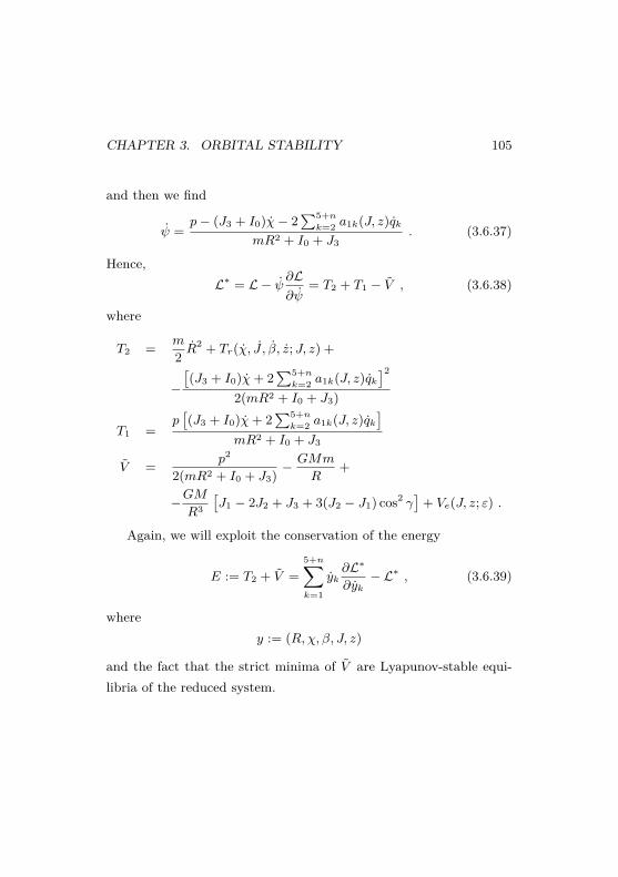
CHAPTER 3. ORBITAL STABILITY 105
and then we find
ψ =p− (J3 + I0)χ− 2
∑5+nk=2 a1k(J, z)qk
mR2 + I0 + J3. (3.6.37)
Hence,L∗ = L − ψ ∂L
∂ψ= T2 + T1 − V , (3.6.38)
where
T2 = m
2 R2 + Tr(χ, J , β, z; J, z) +
−[(J3 + I0)χ+ 2
∑5+nk=2 a1k(J, z)qk
]22(mR2 + I0 + J3)
T1 =p[(J3 + I0)χ+ 2
∑5+nk=2 a1k(J, z)qk
]mR2 + I0 + J3
V = p2
2(mR2 + I0 + J3) −GMm
R+
−GMR3
[J1 − 2J2 + J3 + 3(J2 − J1) cos2 γ
]+ Ve(J, z; ε) .
Again, we will exploit the conservation of the energy
E := T2 + V =5+n∑k=1
yk∂L∗
∂yk− L∗ , (3.6.39)
wherey := (R,χ, β, J, z)
and the fact that the strict minima of V are Lyapunov-stable equi-libria of the reduced system.

CHAPTER 3. ORBITAL STABILITY 106
Let R0 be a nondegenerate minimum of the function
VG0(R) := −GMm
R+ p2
2(mR2 + I0) . (3.6.40)
Then we have the following
Lemma 3.6.17. For any ε small enough there exist R, J , z, s.t.
(1) the manifold
M :=
(R, χ, β, J1, J2, J3, z)|χ+ β = 0,
is composed by critical points of V .
(2) M is a minimum of V which is nondegenerate in the transversaldirection.
(3) One has (J , z) = O(ε) and |R−R0| = O(ε).
(4) Finally J1 < J2 < J3.
Remark 3.6.18. Point (4) guarantees that M ⊂ C6=. If ε is suffi-ciently small, then we haveM⊂ F .
Remark 3.6.19. M is the manifold corresponding to 1:1 spin orbitresonance.
Proof. We look for a minimum of V in the domain J1 ≤ J2 and|J | ≤ Cε for some fixed C.

CHAPTER 3. ORBITAL STABILITY 107
First remark that, as a function of γ = χ+ β, V has a minimumat γ=0 (strict if J1 < J2). Consider now V
∣∣γ=0
; as a function of Rit has a nondegenerate minimum at some point R = R(J, z) fulfilling
|R(J, z)−R0| ≤ Cε .
Consider now the restriction V = V (J, z) of V to the manifold γ = 0,R = R(J, z); since
V (J, z) = 1ε
[Q(J, z) + V3(J, z)] +O(1) , (3.6.41)
such a function has a nondegenerate minimum close to zero.Then (1), (2) and (3) follow provided one shows that J1 < J2.
We are now going to prove (4) which in particular implies the thesis.To this end, observe that at the critical point one has
0 = ∂V
∂J1= 2GM
R3+ A
εJ1 + B
ε(J2 + J3) + 1
ε
+∞∑j=1
Cj zj +O(ε) (3.6.42)
0 = ∂V
∂J2= −GM
R3+A
εJ2+B
ε(J1+J3)+ 1
ε
+∞∑j=1
Cj zj+O(ε) . (3.6.43)
0 = ∂V
∂J3= − p2
2(mR2 + I0 + J3)2− GM
R3+
+A
εJ3 + B
ε(J1 + J2) + 1
ε
+∞∑j=1
Cj zj +O(ε) . (3.6.44)
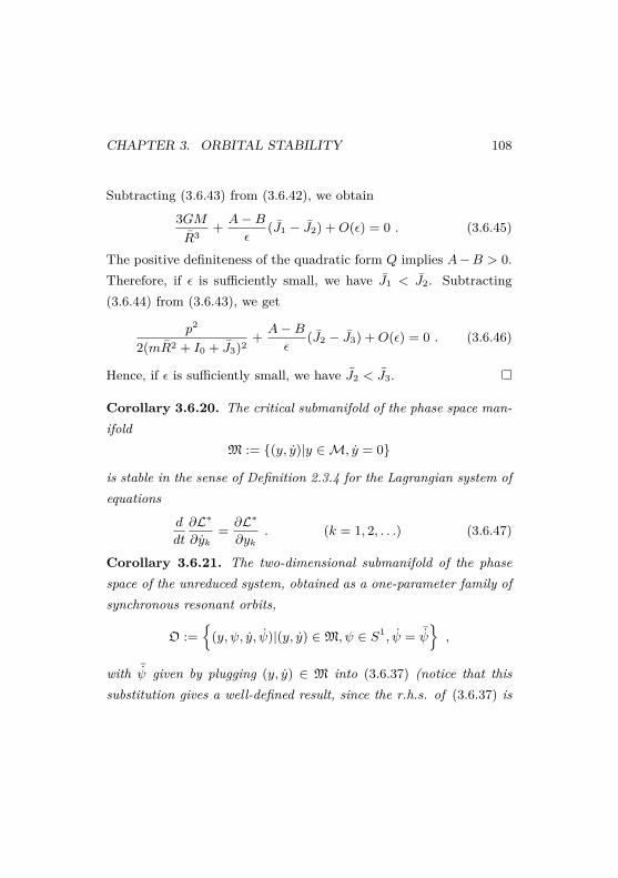
CHAPTER 3. ORBITAL STABILITY 108
Subtracting (3.6.43) from (3.6.42), we obtain
3GMR3
+ A−Bε
(J1 − J2) +O(ε) = 0 . (3.6.45)
The positive definiteness of the quadratic form Q implies A−B > 0.Therefore, if ε is sufficiently small, we have J1 < J2. Subtracting(3.6.44) from (3.6.43), we get
p2
2(mR2 + I0 + J3)2+ A−B
ε(J2 − J3) +O(ε) = 0 . (3.6.46)
Hence, if ε is sufficiently small, we have J2 < J3.
Corollary 3.6.20. The critical submanifold of the phase space man-ifold
M := (y, y)|y ∈M, y = 0
is stable in the sense of Definition 2.3.4 for the Lagrangian system ofequations
d
dt
∂L∗
∂yk= ∂L∗
∂yk. (k = 1, 2, . . .) (3.6.47)
Corollary 3.6.21. The two-dimensional submanifold of the phasespace of the unreduced system, obtained as a one-parameter family ofsynchronous resonant orbits,
O :=
(y, ψ, y, ψ)|(y, y) ∈M, ψ ∈ S1, ψ = ¯ψ,
with ¯ψ given by plugging (y, y) ∈ M into (3.6.37) (notice that thissubstitution gives a well-defined result, since the r.h.s. of (3.6.37) is
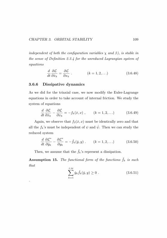
CHAPTER 3. ORBITAL STABILITY 109
independent of both the configuration variables χ and β), is stable inthe sense of Definition 2.3.4 for the unreduced Lagrangian system ofequations
d
dt
∂L∂xk
= ∂L∂xk
. (k = 1, 2, . . .) (3.6.48)
3.6.6 Dissipative dynamics
As we did for the triaxial case, we now modify the Euler-Lagrangeequations in order to take account of internal friction. We study thesystem of equations
d
dt
∂L∂xk− ∂L∂xk
= −fk(x, x) , (k = 1, 2, . . .) (3.6.49)
Again, we observe that f2(x, x) must be identically zero and thatall the fk’s must be independent of ψ and ψ. Then we can study thereduced system
d
dt
∂L∗
∂yk− ∂L∗
∂yk= −fk(y, y) . (k = 1, 2, . . .) (3.6.50)
Then, we assume that the fk’s represent a dissipation.
Assumption 15. The functional form of the functions fk is suchthat
+∞∑k=1
ykfk(y, y) ≥ 0 . (3.6.51)
.

CHAPTER 3. ORBITAL STABILITY 110
Then, the usual reasoning about non-increasing energy, togetherwith Lemma 3.5.7, gives the result of orbital stability of the syn-chronous resonance, in the following sense.
Theorem 3.6.22. The manifold M is stable in the future, in thesense of Definition 2.3.4, for the reduced system of equations (3.6.50).
Corollary 3.6.23. The manifold O of synchronous resonant circularorbits is orbitally stable in the future, in the sense of Definition 2.3.4,for the unreduced system of equations (3.6.49).
3.6.7 Multi-layer satellite
We remark that the proof of the orbital stability that we have givenfor a spherically symmetric satellite can be immediately extended tothe case of amulti-layer spherically symmetric satellite. A sphericallysymmetric satellite with n layers has the following structure in thereference configuration: the inner layer (the core) is a sphere, whilethe n − 1 outer layers are spherical shells, adjacent to one another.These n layers are free to slide (possibly with some dissipation ofenergy) on one another. Moreover, we require the same properties ofinvariance of the Lagrangian function as for the “single-layer” case.
All the machinery works exactly the same way, except some tech-nical details. In this case, it is convenient to use the group actions A1
andA3, instead ofA1 andA2. Then, observe thatA1[R(α)]A2[R(β)] =A1[R(α + β)]A3[R(−β)]. Then, when passing to the quotient, one
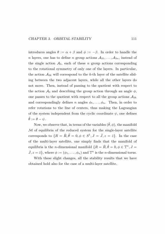
CHAPTER 3. ORBITAL STABILITY 111
introduces angles θ := α + β and φ := −β. In order to handle then layers, one has to define n group actions A31, . . . ,A3n, instead ofthe single action A3, each of these n group actions correspondingto the rotational symmetry of only one of the layers. In particular,the action A3k will correspond to the k-th layer of the satellite slid-ing between the two adjacent layers, while all the other layers donot move. Then, instead of passing to the quotient with respect tothe action A3 and describing the group action through an angle φ,one passes to the quotient with respect to all the group actions A3k
and correspondingly defines n angles φ1, . . . , φn. Then, in order torefer rotations to the line of centers, thus making the Lagrangianof the system independent from the cyclic coordinate ψ, one definesθ := θ − ψ.
Now, we observe that, in terms of the variables (θ, φ), the manifoldM of equilibria of the reduced system for the single-layer satellitecorresponds to R = R, θ = 0, φ ∈ S1, J = J , z = z. In the caseof the multi-layer satellite, one simply finds that the manifold ofequilibria is the n-dimensional manifold R = R, θ = 0, φ ∈ Tn, J =J , z = z, where φ := (φ1, . . . , φn) and Tn is the n-dimensional torus.
With these slight changes, all the stability results that we haveobtained hold also for the case of a multi-layer satellite.

CHAPTER 3. ORBITAL STABILITY 112
3.7 General comments
We recall the theorem of the three outcomes that we have proved inthe previous chapter: one of the consequences was that, if there isorbital stability of the synchronous resonance, then the synchronousresonance is also asymptotically stable. The results of orbital stabilitythat we have proved in the present chapter are not a completelyrigorous proof of the asymptotic stability, since in the present chapterwe have done some approximations. If the same result of the orbitalstability that we have obtained in this chapter were proved removingour approximations, then the asymptotic stability of the synchronousresonance would be automatically proved through the theorem of thethree outcomes.
A further comment is worth being done about the result of sta-bility that we have obtained for a spherically symmetric satellite: weare not able to prove that each of the synchronous resonant orbitsof the manifold O is orbitally stable, when considered alone. Evenif we have proved that the speed of rotation of the satellite tends tozero, we are unable to prove that asymptotically “the satellite stopsrotating”: we only prove that asymptotically the principal axes of in-ertia stop rotating. This is compatible with a situation in which thesatellite has a constant shape, but the direction of the deformationcontinuously changes in the body. In a pictorial way one can thinkof a rubber balloon which on a wooden cross whose axes are fixed inspace. In a more rigorous fashion, we are stating that the previous

CHAPTER 3. ORBITAL STABILITY 113
theorem implies that χ + β → 0 when t → +∞, but it says nothingabout the individual behavior of χ and β. If there is asymptotic sta-bility, then this implies that χ and β approach zero as t→ +∞ (therubber balloon slides on the wooden cross more and more slowly).This, however, does not imply that there exist χ and β such thatχ → χ or that β → β, since, at our level of generality, we are notable to prove the convergence of the integrals∫ +∞
0χ(t)dt
∫ +∞
0β(t)dt .
3.8 A direct proof of the asymptotic stability
In this section, we show that, under some more assumptions andapproximations, in the spherically symmetric case it is possible togive a proof of the asymptotic stability, directly from the equationsof motion.
The further approximation that we impose here is a finite-dimen-sionality approximation.
Assumption 16 (Finite-dimensionality). The space C is finite-di-mensional.
We are assuming that the dimension of C is arbitrary, but finite.For example, one can obtain this by cutting at any order the multi-pole expansion of the configuration v ∈ C. The Lagrangian variables(z1, z2, . . .) will therefore be replaced by (z1, z2, . . . , zn).

CHAPTER 3. ORBITAL STABILITY 114
Under this finite-dimensionality assumption, we can prove a usefulresult about the expression of the kinetic energy.
Lemma 3.8.1. The coefficient a12(J, z) satisfies:
lim(J,z)→0
a12(J, z) = 0 . (3.8.1)
Proof. We use the same notation as in Lemma 3.6.16. Then, reason-ing as in the proof of Lemma 3.6.16, we observe that the coefficienta12 of the term αβ in the expression of the kinetic energy arises fromthe integral ∫
Ω〈ω × u(x), u(x)〉ρ(x)d3x
in (3.6.34). The α factor comes from the angular velocity ω, whilethe β factor is hidden in u(x). Define
wdef = w − v0 = A2[R(−β)]u− v0 . (3.8.2)
We get
u(x) = R(β) wdef [R(−β)x]+ β∂R(β)∂β
wdef [R(−β)x] +
+βR(β)∇wdef [R(−β)x] · ∂R(−β)∂β
x . (3.8.3)
Here, we notice that the first of the three addenda is independent ofβ (since w = wdef + v0 belongs to the section S, which is transversalto the group action A2), so we have (exploiting v0(x) = x)
a12(J, z) = 12
∫Ωρ(x)〈u3 × x +R(β)wdef [R(−β)x], (3.8.4)
∂R(β)∂β
wdef [R(−β)x] +R(β)∇wdef [R(−β)x] · ∂R(−β)∂β
x〉d3x ,

CHAPTER 3. ORBITAL STABILITY 115
which goes to zero when wdef → 0, i.e. when (J, z)→ 0; this is wherewe exploit the assumption of finite-dimensionality, since we use theequivalence of norms (wdef → 0⇔ ∇wdef → 0).
Moreover, we will make some more assumption about the dissipa-tive terms in the equations of motion, i.e. we introduce a Rayleigh’sdissipation function F (y; y). Namely, we assume that the equationsof motion of the reduced system have the form (3.8.5) below. Ofcourse, we do not expect dissipation to act directly on the orbitalvariables R and χ, so we assume F to be independent of R, χ, R andχ. Due to the A2-invariance of the satellite, F is also independent ofthe coordinate β (but it depends on β); however, for the proof of ourresult, it is not necessary that F be β-independent.
Assumption 17. As a function of the velocities (β, J , z), the Rayleigh’sdissipation function F (β, J , z; J, z) has a nondegenerate minimum at0.
We denote by ye := (β, J, z) the variables fixing the configura-tion of the satellite. So in particular we have F = F (ye, ye) (with∂F/∂β = 0).
Then the result of asymptotic stability is:
Theorem 3.8.2. If ε is sufficiently small, the manifold M, definedin Section 3.6, is asymptotically stable for the dynamical system ofequations
d
dt
∂L∗
∂yk− ∂L∗
∂yk= − ∂F
∂yk, (k = 1, 2, . . .) (3.8.5)

CHAPTER 3. ORBITAL STABILITY 116
with L∗ defined as in Section 3.6.
Proof. Let us evaluate the time derivative of the energy:
dE
dt= d
dt
(4+n∑k=1
yk∂L∗
∂yk
)− d
dtL∗ =
=4+n∑k=1
yk∂L∗
∂yk+
4+n∑k=1
ykd
dt
∂L∗
∂yk−
4+n∑k=1
yk∂L∗
∂yk−
4+n∑k=1
yk∂L∗
∂yk=
= −4+n∑k=1
yk∂F
∂yk= −
(2QF +
4+n∑k=1
yk∂F3
∂yk
), (3.8.6)
where QF is the quadratic part of F , and F3 is the part of order 3 inye. Let ND := (y, y)|F (y; y) = 0 =
(y, y)|β = J = z = 0
be the
subset of phase space where there is no energy dissipation. Then, dueto LaSalle’s invariance principle, any solution such that (y(0), y(0))belongs to a sufficiently small neighborhood of M (notice that sucha solution will stay bounded for all t ≥ 0 due to the stability of Mproved in Section 3.6) will get arbitrarily close to the largest invariantsubset of ND, for t → +∞. Therefore, the only thing we have tocheck is that the set ND contains no orbit, apart from the points ofthe manifoldM. To check this, observe that, if such an orbit existed,it would satisfy equations (3.8.5). In particular, the orbit satisfies
d
dt
∂L∗
∂χ− ∂L∗
∂χ= 0 (3.8.7)
andd
dt
∂L∗
∂β− ∂L∗
∂β= −∂F
∂β. (3.8.8)

CHAPTER 3. ORBITAL STABILITY 117
When restricting to ND, these two equations become, respectively,
− (I0 + J3)2χ
mR2 + I0 + J3+ 2mR(I0 + J3)2χR
(mR2 + I0 + J3)2 + (3.8.9)
+(I0 + J3)χ− 2pmR(I0 + J3)R(mR2 + I0 + J3)2 = −∂V
∂χ(y)
and
−a12(J, z)(I0 + J3)χmR2 + I0 + J3
+ 2mRa12(J, z)(I0 + J3)χR(mR2 + I0 + J3)2 + (3.8.10)
+a12(J, z)χ− 2pmRa12(J, z)R(mR2 + I0 + J3)2 = −∂V
∂β(y) ,
where we took into account that, by Assumption 17, ∂F/∂β vanishesonM. Observe that the r.h.s.’s of the two equations are equal.
Multiplying (3.8.9) by a12(J,z)I0+J3
and subtracting (3.8.10) we get(1− a12
I0 + J3
)∂V
∂γ= 0 ,
which, by (3.8.1), implies ∂V∂γ
= 0, and therefore χ+β = 0. Then, wehave χ = −β = 0, since β = 0 on ND. Now , substituting χ = χ = 0into equations (3.8.9) and (3.8.10), we find R = 0. Finally, we observethat now we have
χ = β = R = J = z = 0 , (3.8.11)
which is true on the equilibrium manifoldM only.We have thus proved that the only orbits contained in ND are the
points of the synchronous resonance manifoldM, which, by LaSalle’sinvariance principle, implies the asymptotic stability ofM.

Bibliography
[1] M. E. Alexander. The Weak Friction Approximation and TidalEvolution in Close Binary Systems. Astrophysics and Space Sci-ence, 23:459–510, 1973.
[2] D. Bambusi, E. Haus. Asymptotic stability of spin or-bit resonance for the dynamics of a viscoelastic satellite.http://arxiv.org/abs/1012.4974.
[3] D. Bambusi, E. Haus. Asymptotic stabiity of the synchronousresonance for an elastic satellite with friction. work in progress.
[4] A. Celletti and L. Chierchia. Hamiltonian stability of spin-orbitresonances in celestial mechanics. Celestial Mech. Dynam. As-tronom., 76(4):229–240, 2000.
118

BIBLIOGRAPHY 119
[5] A. Celletti and L. Chierchia. Quasi-periodic attractors in ce-lestial mechanics. Arch. Ration. Mech. Anal., 191(2):311–345,2009.
[6] A. Celletti, C. Froeschlé, and E. Lega. Dynamics of the conser-vative and dissipative spin orbit problem. Planetary and SpaceScience, 55:889–899, 2007.
[7] S. Chandrasekhar. Ellipsoidal Figures of Equilibrium, Chap.VIII. Yale University Press, New Haven, 1969.
[8] A. C. M. Correia and J. Laskar. Mercury’s capture into the 3/2spin-orbit resonance as a result of its chaotic dynamics. Nature,429:848–850, 2004.
[9] G. H. Darwin. On the Precession of a Viscous Spheroid, andon the Remote History of the Earth. Royal Society of LondonPhilosophical Transactions Series I, 170:447–538, 1879.
[10] G. H. Darwin. On the Secular Changes in the Elements of theOrbit of a Satellite Revolving about a Tidally Distorted Planet.Royal Society of London Philosophical Transactions Series I,171:713–891, 1880.
[11] M. Efroimsky and J. G. Williams. Tidal torques. A critical re-view of some techniques. Celestial Mechanics and DynamicalAstronomy, 104:257–289, 2009.
BIBLIOGRAPHY 120
[12] M. Efroimsky. Bodily tides near spin-orbit resonances. submit-ted to Celestial Mechanics and Dynamical Astronomy, 2011.
[13] S. Ferraz-Mello, A. Rodríguez, and H. Hussmann. Tidal fric-tion in close-in satellites and exoplanets: The Darwin the-ory re-visited. Celestial Mechanics and Dynamical Astronomy,101:171–201, 2008.
[14] J. Getino, A. Escapa, and A. García. Spheroidal and toroidalmodes for tidal kinetic energy in axisymmetric, slightly ellipti-cal, elastic bodies. Romanian Astronomical Journal, 13:143–161,2003.
[15] P. Goldreich. Final spin states of planets and satellites. Astro-nomical Journal, 71:1–7, 1966.
[16] P. Goldreich. History of the Lunar orbit Reviews of Geophysics,4:411–439, 1966.
[17] P. Goldreich and S. Peale. Spin-orbit coupling in the Solar Sys-tem Astronomical Journal, 71:425–438, 1966.
[18] A. Hatcher. Algebraic topology. Cambridge University Press,Cambridge, 2002.
[19] E. Haus. Asymptotic behavior of an elastic satellite with friction.work in progress.

BIBLIOGRAPHY 121
[20] W. M. Kaula. Tidal Dissipation by Solid Friction and the Result-ing Orbital Evolution. Reviews of Geophysics and Space Physics,2:661–685, 1964.
[21] G. A. Krasinsky. Dynamical hystory of the Earth-Moon system.Celestial Mechanics and Dynamical astronomy, 84:27–55, 2002.
[22] G. A. Krasinsky. Numerical theory of rotation of the deformableEarth with the two layer fluid core. Part 1: mathematicalmodel. Celestial Mechanics and Dynamical astronomy, 96:169–217, 2006.
[23] J. P. LaSalle. The stability of dynamical systems. Society forIndustrial and Applied Mathematics, Philadelphia, Pa., 1976.With an appendix: “Limiting equations and stability of nonau-tonomous ordinary differential equations” by Z. Artstein, Re-gional Conference Series in Applied Mathematics.
[24] A. E. H. Love. A treatise on the mathematical theory of elasticity.CUP, Cambridge, 1927.
[25] G. J. F. MacDonald. Tidal Friction. Reviews of Geophysics andSpace Physics, 2:467–541, 1964.
[26] J. E. Marsden and Thomas J. R. Hughes. Mathematical foun-dations of elasticity. Dover Publications Inc., New York, 1994.Corrected reprint of the 1983 original.

BIBLIOGRAPHY 122
[27] F. Mignard. The evolution of the lunar orbit revisited I. MoonPlanets, 20:301–315, 1979.
[28] F. Mignard. The evolution of the lunar orbit revisited II. MoonPlanets, 23:185–201, 1980.
[29] O. Neron de Surgy and J. Laskar. On the long term evolution ofthe spin of the Earth. Astronomy and Astrophysics, 318:975–989,1997.
[30] S. J. Peale, P. Cassen, and R. T. Reynolds. Tidal dissipation,orbital evolution, and the nature of Saturn’s inner satellites.Icarus, 43:65–72, 1980.
[31] A. V. Shatina. Evolution of the Motion of a Viscoelastic Spherein a Central Newtonian Field. Cosmic Research, 39:282–294,2001. 10.1023/A:1017585722391.
[32] S. F. Singer. The origin of the Moon and geophysical conse-quences Geophysical Journal of the Royal Astronomical Society,15:205–226, 1968.
[33] J.-J. Tisserand. Traité de Mécanique Céleste, tome II, chap. VIIIGauthier Villars, Paris, 1891.
[34] J. Touma and J. Wisdom. Evolution in the Earth-Moon system.Astronomical Journal, 108:1942–1961, 1994.

BIBLIOGRAPHY 123
[35] V. G. Vil’Ke, S. A. Kopylov, and Y. G. Markov. Evolution of therotation of a viscoelastic planet on a circular orbit in a centralforce field. Soviet Astronomy, 28:702–705, 1984.