ensemble model output statistics for wind vectorsthordis/files/schuhen2011.pdf · ensemble model...
TRANSCRIPT

Ruprecht-Karls-Universität Heidelberg
Fakultät für Mathematik und Informatik
Ensemble Model Output Statisticsfor Wind Vectors
Diplomarbeitvon
Nina Schuhen
Betreuer: Prof. Dr. Tilmann GneitingDr. Thordis L. Thorarinsdottir
September 2011


Zusammenfassung
Through the advent of ensemble forecasts, weather prediction experienced a systematic shiftfrom the traditional deterministic view to a modern probabilistic approach. These ensembles,multiple runs of one or more mathematical models, however are often underdispersive, as onlysome of the uncertainties involved in numerical weather prediction are captured. Thereforestatistical postprocessing methods were developed to transform discrete ensemble outputinto calibrated and sharp predictive distributions. So far these techniques only applied toone-dimensional weather quantities like temperature, air pressure or precipitation. In thisthesis, we present a bivariate approach to address ensemble forecasts of two-dimensionalwind vectors, extending the well-established EMOS method. We preserve its essential benefitsand model the correlation between the vector components as a trigonometric function of thepredicted wind direction. Additionally, our new method is tested against other forecastingtechniques, using the UWME ensemble over the North American Pacific Northwest.
Zusammenfassung
Durch das Aufkommen von Ensemblevorhersagen hat die Wettervorhersage einen systemati-schen Wandel weg vom traditionell deterministischen und hin zu einem modernen probabilisti-schen Ansatz erlebt. Diese Ensembles, mehrere Durchläufe eines oder mehrerer mathematischerModelle, sind jedoch oft unterdispersiv, weil nur einige der Unsicherheiten, die mit numerischerWettervorhersage einhergehen, berücksichtigt werden. Daher wurden statistische Aufberei-tungsmethoden entwickelt, um den diskreten Ensembleoutput in kalibrierte und scharfeWahrscheinlichkeitsverteilungen umzuwandeln. Bisher ließen sich diese Verfahren jedoch nurauf eindimensionale Wettergrößen wie Temperatur, Luftdruck oder Niederschlag anwenden.In dieser Arbeit stellen wir eine bivariate Herangehensweise vor, die die bekannte EMOSMethode erweitert und sich mit Ensemblevorhersagen für zweidimensionale Windvektorenbeschäftigt. Dabei behalten wir die grundlegenden Eigenschaften des univariaten Verfahrensbei und modellieren die Korrelation zwischen den Vektorkomponenten als eine trigonometrischeFunktion der vorhergesagten Windrichtung. Des Weiteren führen wir eine Fallstudie für dasUWME Ensemble über dem nordamerikanischen Pazifischen Nordwesten durch und testenunsere neue Methode gegen andere Vorhersageverfahren.
3

Contents
1 Introduction 7
2 Assessing Forecast Skill 152.1 Assessing Calibration . . . . . . . . . . . . . . . . . . . . . . . . . . . . . . . . 16
2.1.1 Univariate Histograms . . . . . . . . . . . . . . . . . . . . . . . . . . . 162.1.2 Multivariate Rank Histogram . . . . . . . . . . . . . . . . . . . . . . . 182.1.3 Marginal Calibration Diagram . . . . . . . . . . . . . . . . . . . . . . . 20
2.2 Assessing Sharpness . . . . . . . . . . . . . . . . . . . . . . . . . . . . . . . . . 212.3 Proper Scoring Rules . . . . . . . . . . . . . . . . . . . . . . . . . . . . . . . . 22
2.3.1 Univariate Forecasts . . . . . . . . . . . . . . . . . . . . . . . . . . . . 232.3.2 Multivariate Forecasts . . . . . . . . . . . . . . . . . . . . . . . . . . . 24
3 EMOS for Univariate Weather Quantities 273.1 General Idea . . . . . . . . . . . . . . . . . . . . . . . . . . . . . . . . . . . . . 273.2 Standard EMOS . . . . . . . . . . . . . . . . . . . . . . . . . . . . . . . . . . 28
3.2.1 EMOS+ . . . . . . . . . . . . . . . . . . . . . . . . . . . . . . . . . . . 303.3 EMOS for Wind Speed . . . . . . . . . . . . . . . . . . . . . . . . . . . . . . . 313.4 EMOS for Wind Gust . . . . . . . . . . . . . . . . . . . . . . . . . . . . . . . 32
4 Extending EMOS to Wind Vector Forecasts 354.1 Properties of Wind Vectors . . . . . . . . . . . . . . . . . . . . . . . . . . . . . 364.2 EMOS for Wind Vectors . . . . . . . . . . . . . . . . . . . . . . . . . . . . . . 37
4.2.1 Data Analysis . . . . . . . . . . . . . . . . . . . . . . . . . . . . . . . . 38
5

CONTENTS
4.2.2 Modelling the predictive distribution . . . . . . . . . . . . . . . . . . . 414.2.3 The Mean Vector and Linear Regression . . . . . . . . . . . . . . . . . 434.2.4 The Correlation Coefficient and the Wind Direction . . . . . . . . . . . 464.2.5 The Variances and Maximum Likelihood . . . . . . . . . . . . . . . . . 49
5 Case Study and Predictive Performance 535.1 The University of Washington Mesoscale Ensemble . . . . . . . . . . . . . . . 535.2 Regional and Local EMOS Technique . . . . . . . . . . . . . . . . . . . . . . . 56
5.2.1 Regional EMOS . . . . . . . . . . . . . . . . . . . . . . . . . . . . . . . 575.2.2 Local EMOS . . . . . . . . . . . . . . . . . . . . . . . . . . . . . . . . 59
5.3 Competing Forecasts . . . . . . . . . . . . . . . . . . . . . . . . . . . . . . . . 625.3.1 Climatological Ensemble . . . . . . . . . . . . . . . . . . . . . . . . . . 625.3.2 Error Dressing Ensemble . . . . . . . . . . . . . . . . . . . . . . . . . . 635.3.3 EMOS for Wind Vector Components . . . . . . . . . . . . . . . . . . . 645.3.4 ECC Ensemble . . . . . . . . . . . . . . . . . . . . . . . . . . . . . . . 655.3.5 Converting Ensemble and Density Forecasts . . . . . . . . . . . . . . . 66
5.4 Predictive Performance for Wind Vector Forecasts . . . . . . . . . . . . . . . . 675.4.1 Results for Sea-Tac Airport, 23 January 2008 . . . . . . . . . . . . . . 675.4.2 Results for Sea-Tac Airport, 1 January - 31 December 2008 . . . . . . . 725.4.3 Results for the Pacific Northwest, 1 January - 31 December 2008 . . . . 77
5.5 Predictive Performance for Wind Speed Forecasts . . . . . . . . . . . . . . . . 89
6 Summary and Discussion 95
A Local Correlation Curves 99
B List of Notation for Chapter 4 120
6

Chapter 1
Introduction
Prediction is very difficult, especially about the future.Often attributed to Nobel laureate Niels Bohr (1885-1962)
Although predicting the future might be difficult, modern forecasting is perceived as a matterof great importance. In the process of making statements and inferences about the things tocome, we draw on experiences from the past, often in form of statistics. Over the last decades,major aims of statistical analysis have become not only to make forecasts, but also to measurethe associated uncertainty. Therefore, they should be expressed as probability distributions(Dawid 1984).
Many forecasts, however, are of deterministic nature, may it be for reasons of communicationor decision making (Gneiting 2011). Still, a transition to probabilistic forecasts is in progressand statisticians function as a driving force (Gneiting 2008). The goal is not to eliminate, butto assess and evaluate uncertainty.
In meteorology, the probability of precipitation has been an integral part of most weatherforecasts for a number of years. Yet, people often don’t understand how to interpret such apercentage (Gigerenzer et al. 2005). But especially in this field, the probabilistic approachis very effective for a number of practical applications. Probabilities of exceeding a certain
7

CHAPTER 1. Introduction
threshold are used for issuing severe weather warnings, maintaining air and shipping trafficregulations, or for efficient agriculture as the risk of freezing temperatures. Palmer (2002)points out that weather and climate predictions have an enormous potential economic value:Financial profit can be traded off against the probability of heavy losses due to e.g. extremeweather.
Customers often have the choice between multiple forecasting products. But how do werank rivalling forecasters? How can the “best” prediction be determined? Gneiting et al. (2007)proposed the principle of maximising the sharpness of a probabilistic forecast subject to itscalibration. Calibration refers to the reliability of the forecast, i.e. the statistical consistencybetween the predictive probability distribution and the actually occurring observations. Sharp-ness quantifies the concentration of the distribution; under the condition that all forecasts arecalibrated, we define the sharpest forecast to be the best.
Numerical weather prediction (NWP) simplified the process of incorporating probabilisticmethods into traditional weather forecasting. The grid-based NWP models consist of anumber of dynamical partial differential equations which are discretised and integrated forwardto obtain future states of the atmosphere. The current state is assimilated from actualobservations and provides the initial and lateral boundary conditions for these models.
Until the 1990s, one mathematical model was supplied with the one set of input data, whichwas deemed best to represent the current atmosphere (Gneiting and Raftery 2005). Chaostheory, however, implies that little deviations in the initial conditions can lead to significantforecast errors, as the observations are subject to a certain degree of imprecision. One reasonfor this is that observational locations are irregularly placed, and there are many areas withonly sparse observational data, especially over the oceans. Interpolation to the grid structuretherefore causes inherent uncertainties, which again limits the predictability, however skillfulthe model might be (Grimit 2001).
NWP models, on the other hand, became more and more accurate over time. In order tocapture small-scale processes, the grid resolution was increased constantly. For instance, theCOSMO-DE model of the German Weather Service (DWD), operational since 2007, has ahorizontal spacing of 2.8 km (Baldauf et al. 2011). Despite the latest developments, however,there are limitations to the computer resources which are needed for such models.
8

CHAPTER 1. Introduction
Today, numerical weather prediction has changed from being a deterministic matter tothe probabilistic approach of ensemble forecasting (see e.g. Leutbecher and Palmer 2008).Ensembles consist of multiple point forecasts, named ensemble members, generated by NWPmodels and can be ordered into three groups:
• Multianalysis ensembles:One numerical model is run multiple times, using slightly different sets of initial condi-tions.
• Multimodel ensembles:Multiple numerical models are run with a single set of initial conditions.
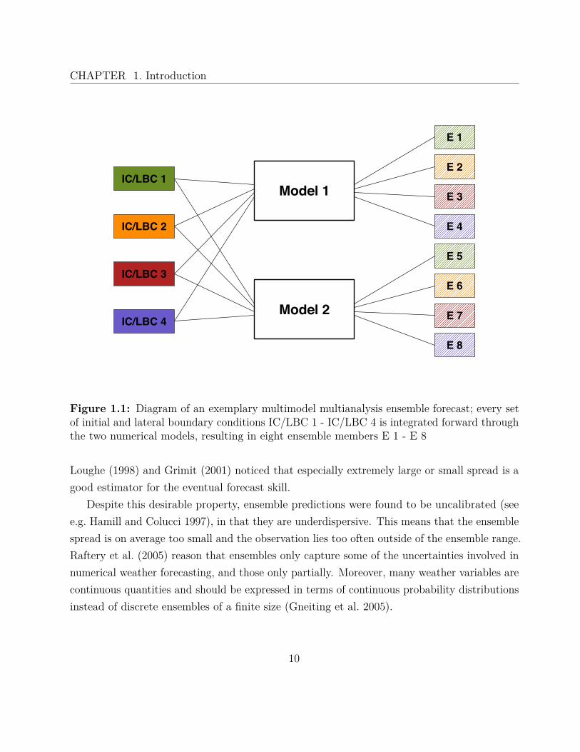
• Multimodel multianalysis ensembles:As a combination of the previous ones, multiple sets of initial conditions are used to runmultiple numerical models.
In this way, the two major uncertainty sources are addressed: the imperfections in theinitial conditions and the inadequacies of the mathematical models. Ensemble predictionsystem have been implemented for both short-range (0-48 hours) and medium-range (2-10days) weather forecasting (Eckel and Mass 2005), in the form of regional and global NWPmodels, respectively. Figure 1.1 shows a schematic representation of an exemplary multimodelmultianalysis ensemble with two models and eight ensemble members. The ensemble picturedin Figure 1.2 is the multianalysis University of Washington Mesoscale Ensemble (UWME), asoperational in 2008. A full description can be found in Section 5.1.
The context of ensemble forecasts provides the possibility of combining a point forecast,say the ensemble mean, with an estimation of its accuracy, through for instance the root meansquared error. On average, the ensemble mean outperforms each of the individual ensemblemembers, in that it is the best estimate for the verifying state of the atmosphere (Grimit andMass 2002).
Another important aspect is the so called spread-error correlation or spread-skill relationshipof the ensemble. Often there exists a link between the a priori known ensemble spread (orensemble variance) and the observed error of the ensemble mean forecast. Whitaker and
9
CHAPTER 1. Introduction
IC/LBC 4
IC/LBC 3
IC/LBC 2
IC/LBC 1
Model 2
Model 1
E 8
E 7
E 6
E 5
E 4
E 3
E 2
E 1
Figure 1.1: Diagram of an exemplary multimodel multianalysis ensemble forecast; every setof initial and lateral boundary conditions IC/LBC 1 - IC/LBC 4 is integrated forward throughthe two numerical models, resulting in eight ensemble members E 1 - E 8
Loughe (1998) and Grimit (2001) noticed that especially extremely large or small spread is agood estimator for the eventual forecast skill.
Despite this desirable property, ensemble predictions were found to be uncalibrated (seee.g. Hamill and Colucci 1997), in that they are underdispersive. This means that the ensemblespread is on average too small and the observation lies too often outside of the ensemble range.Raftery et al. (2005) reason that ensembles only capture some of the uncertainties involved innumerical weather forecasting, and those only partially. Moreover, many weather variables arecontinuous quantities and should be expressed in terms of continuous probability distributionsinstead of discrete ensembles of a finite size (Gneiting et al. 2005).
10

CHAPTER 1. Introduction
UKMO
TCWB
NGPS
JMA
GASP
ETA
CMCG
AVN
MM5 Model
UKMO−MM5
TCWB−MM5
NGPS−MM5
JMA−MM5
GASP−MM5
ETA−MM5
CMCG−MM5
AVN−MM5
Figure 1.2: Diagram of the UWME; eight different sets of initial and boundary conditions (onthe left) are integrated forward using the MM5 numerical model, resulting in eight ensemblemembers (on the right)
All these problems, as well as model biases and different spatial resolutions of forecast gridand observations, can be addressed with statistical postprocessing (Gneiting and Raftery 2005).Several such methods have been suggested, with ensemble model output statistics (EMOS) andBayesian model averaging (BMA) being the most prominent. EMOS, elaborately discussedin the next chapter, is based on multiple linear regression and fits a normal distribution tothe ensemble member forecasts. BMA assigns probability density functions to the individualensemble members and generates a weighted average of these densities, where the weightsreflect the forecasting skill of the respective ensemble members. More information about BMAcan be found in Raftery et al. (2005), Sloughter et al. (2007), Sloughter et al. (2010) and Baoet al. (2010).
11
CHAPTER 1. Introduction
Both methods apply to a number of different weather variables like temperature, airpressure or wind speed, however these are only univariate quantities. Surface wind, in contrast,is measured in two dimensions, either as zonal and meridional vector components or as windspeed and wind direction. The application of wind vector forecasts ranges over many differentfields: Air traffic control relies on short-ranged local and regional forecasts, not only to warnof extreme weather, but also to optimise the coordination of runways. For ship routeing,especially probabilistic wind forecasts have a huge economic value, as it can avoid delaysand save fuel. Finally, one of the most important purposes is the production of wind energy;here, the combination of wind speed forecasts, to estimate the production amount, and winddirection forecasts, to adjust the turbines, plays a significant role.
So far, those two variables were always addressed separately (Bao et al. 2010; Sloughteret al. 2010; Thorarinsdottir and Gneiting 2010), not taking into account a possible relationship.For the above mentioned applications, particularly the correlation structure might be of crucialconsequence. Therefore we propose a new approach to postprocess ensemble forecasts ofwind vectors jointly, so that spatial properties are inherited from the underlying numericalmodels. We base our method on the aforementioned EMOS and extend it to bivariate weatherquantities, where the correlation between the two vector components is estimated from historicdata.
Current research relating to wind vectors includes a two-dimensional variant of BMA(Sloughter 2009) and a technique to adaptively calibrate wind vector ensembles (Pinson2011). The Ensemble Copula Coupling approach by Schefzik (2011) refers to multidimensionalforecasts in general and can easily be adapted to our task of postprocessing wind vectors.
The new EMOS method will be described and tested as follows:
In Chapter 2, we present several methods to assess the predictive skill of both univariateand multivariate probabilistic forecasts, whether in the form of ensembles or probabilitydistributions. These tools will not only be used to compare performances of forecasts, butare also a part of the parameter estimation, and make sure that the resulting probabilisticforecasts are calibrated and sharp. Here, we refer to Gneiting et al. (2008), where thesemultidimensional assessment tools were described.
12
CHAPTER 1. Introduction
In Chapter 3, the conventional EMOS postprocessing method is discussed in detail. We showall its adaptations and applications and point out the special characteristics and key elements,which will later be incorporated into the bivariate approach.In Chapter 4, we develop the new bivariate method, beginning with an empirical analysis ofdata provided by the UWME ensemble (see Section 5.1). We then propose a model for thebivariate predictive distribution and split the parameter estimation into three parts, therebypredicting forecast mean, correlation and spread successively.In Chapter 5, several other forecasting and postprocessing techniques suitable for wind vectorsare reviewed and we compare the results in form of a case study. The performance of thesemethods is assessed for the North American Pacific Northwest in 2008, using the tools fromChapter 2. For implementing the methods described in this thesis and in order to create thegraphics, the R environment for statistical computing is employed. More information can befound in R Development Core Team (2011).Finally, in Chapter 6, we provide a summary of the new EMOS method for bivariate windvector forecasts and discuss the results of the case study. Also, future prospects are shown,especially in terms of wind field forecasting.
13

Chapter 2
Assessing Forecast Skill
In this chapter, we will present several tools that can be used to assess the forecast skill of thenew EMOS method and of the rivalling forecasting techniques described in Section 5.3. InGneiting et al. (2008), it was established how multivariate ensemble or density forecasts canbe evaluated, so this article will function as a guideline for choosing which tools to use. Oftenthere exists a multidimensional extension to well-known one-dimensional methods, and wewill discuss both univariate and multivariate assessment.
Due to the fact that the thesis at hand concerns wind vectors, we will here focus on forecastassessment in two dimensions. Furthermore, as the new EMOS method will also be used toproduce wind speed forecasts (Section 5.5), the univariate tools are employed in the case studyas well.
Additional to the purpose of assessing forecast skill, so called proper scoring rules are a keyelement of the EMOS postprocessing method itself. As mentioned in the preceding chapter, thegoal of probabilistic forecasting is to maximise the sharpness subject to calibration (Gneitinget al. 2007). Proper scoring rules, elaborately discussed in Gneiting and Raftery (2007), providea way to address both of these properties simultaneously, so a natural conclusion would be toinvolve them in the parameter estimation. Minimum CRPS estimation, for instance, is usedfor the so far known univariate EMOS methods, and we want to find a similar approach forthe bivariate method.
Probabilistic forecasts occur in the form of discrete ensembles or probability densitiesand there are tools that apply to one or the other. However, it does not pose difficulties to
15
CHAPTER 2. Assessing Forecast Skill
draw samples from a predictive distribution and thus create a forecast ensemble, or to fit anappropriate distribution to given ensemble forecasts. In this manner, both types of forecastscan easily be transformed into one another. More details are to be found in Section 5.3.5.
First we take a look at tools to check the calibration of probabilistic forecasts, then thequantification of sharpness will be addressed. In the final section we will introduce severalproper scoring rules, which again will later be used to determine the parameters of the EMOSpredictive distribution.
2.1 Assessing CalibrationCalibration, sometimes referred to as reliability, is a measure for the statistical consistencybetween the probabilistic forecast and the verifying observation. Simply said, this means thatif some event is predicted to occur with a certain probability, say 40%, on average it shouldhappen in about 40% of all times. Thus it is not only a property of the probabilistic forecasts,but also of the verifying observations.
In order to assess the calibration of a forecast, a probability integral transform (PIT) his-togram is usually employed for predictive distributions, while its ensemble forecast counterpartis called verification rank histogram (VRH).
2.1.1 Univariate Histograms
The preferred tool for univariate forecast distributions, the PIT histogram (Dawid 1984;Diebold et al. 1998), is based on the assumption that an observed value x can be perceivedas randomly sampled from a “true” distribution G (Gneiting et al. 2007). If the predicteddistribution F is indeed identical to this true distribution, the value of the predictive cumulativedistribution function (CDF) at x has a uniform distribution
p = F (x) ∼ U [0, 1] .
Therefore, for all forecasts available, the PIT values p are computed, sorted into binsand then formed into a histogram. In this histogram, deviations from uniformity are easy to
16
CHAPTER 2. Assessing Forecast Skill
PIT / Observation Rank
Rel
ative
Fre
quen
cy
Underdispersive Forecast
PIT / Observation Rank
Rel
ative
Fre
quen
cy
Overdispersive Forecast
PIT / Observation Rank
Rel
ative
Fre
quen
cy
Biased Forecast
PIT / Observation Rank
Rel
ative
Fre
quen
cy
Calibrated Forecast
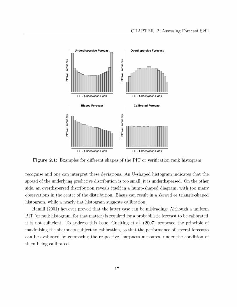
Figure 2.1: Examples for different shapes of the PIT or verification rank histogram
recognise and one can interpret these deviations. An U-shaped histogram indicates that thespread of the underlying predictive distribution is too small, it is underdispersed. On the otherside, an overdispersed distribution reveals itself in a hump-shaped diagram, with too manyobservations in the center of the distribution. Biases can result in a skewed or triangle-shapedhistogram, while a nearly flat histogram suggests calibration.
Hamill (2001) however proved that the latter case can be misleading: Although a uniformPIT (or rank histogram, for that matter) is required for a probabilistic forecast to be calibrated,it is not sufficient. To address this issue, Gneiting et al. (2007) proposed the principle ofmaximising the sharpness subject to calibration, so that the performance of several forecastscan be evaluated by comparing the respective sharpness measures, under the condition ofthem being calibrated.
17

CHAPTER 2. Assessing Forecast Skill
In the context of a discrete ensemble forecast, the verification rank histogram or Talagranddiagram (Anderson 1996; Hamill and Colucci 1997; Talagrand et al. 1997) takes the role ofthe PIT histogram. It relies on the assumption that for a calibrated ensemble of size M ,the observation has the same probability to occupy any rank between 1 and M + 1 whenpooled with the ordered ensemble members. This means, for each time and location, we orderthe ensemble forecasts and observation, find the rank of the observation and finally plot thehistogram of the aggregated ranks. As before, a U-like shape implies underdispersion, whilethe opposite holds for a hump-like shape. Skewed histograms indicate a certain bias andcalibrated ensembles produce a flat histogram. In Figure 2.1, four exemplary histograms areshown.
For comparing different forecasting techniques, it can be useful to quantify the calibration.This is possible with the so-called discrepancy or reliability index ∆ (Delle Monache et al.2006; Berrocal et al. 2007), which is gathered from the respective histograms,
∆ =M+1�
i=1
����fi − 1M + 1
���� .
It measures the deviation between the observed relative frequency fi for bin i and the desiredvalue 1
M+1 , accumulated over all bins.
2.1.2 Multivariate Rank Histogram
A natural generalisation of the VRH to multiple dimensions is the multivariate rank histogram(MRH), the only challenge lies in defining a multivariate rank order. For simplicity reasons,the description below is given for two dimensions, it is however easily applicable to ensembleforecasts of any dimension.
First, we write for two vectors (x1, x2)T and (y1, y2)T
x1
x2
�
y1
y2
if and only if x1 ≤ y1 and x2 ≤ y2.
If we consider the ensemble forecast {xj ∈ R2 : j = 1, . . . , M} and its respective verifyingobservation x0 ∈ R2, we proceed according to the following steps:
18

CHAPTER 2. Assessing Forecast Skill
1. Standardise:It is often useful to apply a principal component transformation to the set{xj : j = 0, . . . , M}, which contains forecasts and observation, thus resultingin standardised values
�x�
j : j = 0, . . . , M�
. In the current context, we refrainfrom doing so.
2. Assign pre-ranks:In the next step, we determine pre-ranks ρj for the possibly standardised valuesx�
j and all j = 0, . . . , M . The pre-rank is defined as
ρj =M�
k=0I
�x�
k � x�j
�,
where I denotes the indicator function. In this way, we find, for each vectorfrom the combined set of ensemble member forecasts and observation, thenumber of vectors from the same set which are smaller or equal in each vectorcomponent. The pre-ranks therefore are integers between 1 and M + 1.
3. Obtain the multivariate rank of the observation:For the multivariate rank r, we note the rank of the observation pre-rank, whilepossible ties are resolved at random. We write
s< =M�
j=0I {ρj < ρ0} and s= =
M�
j=0I {ρj = ρ0}
as the number of pre-ranks that are smaller than the pre-rank of the observationand the number of those that are equal to it. Then r is chosen randomly asany integer between s< + 1 and s< + s=, or more specifically, from a discreteuniform distribution on {s< + 1, . . . , s< + s=}. Again, r can range from 1 toM + 1.
4. Aggregate ranks and plot histogram:For the final step, we aggregate the multivariate ranks over all forecast datesand locations available and plot the histogram of these ranks. To reduce random
19
CHAPTER 2. Assessing Forecast Skill
variability caused by sampling the multivariate rank, the histogram intensitiesare averaged over 100 runs.
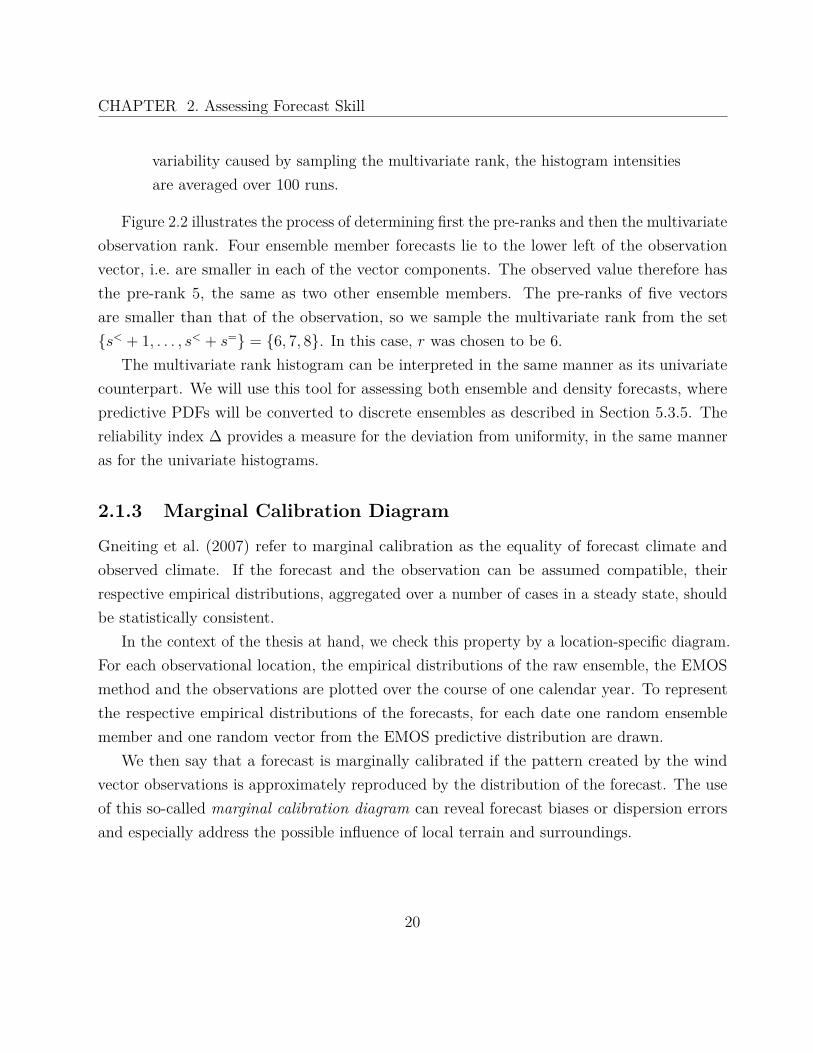
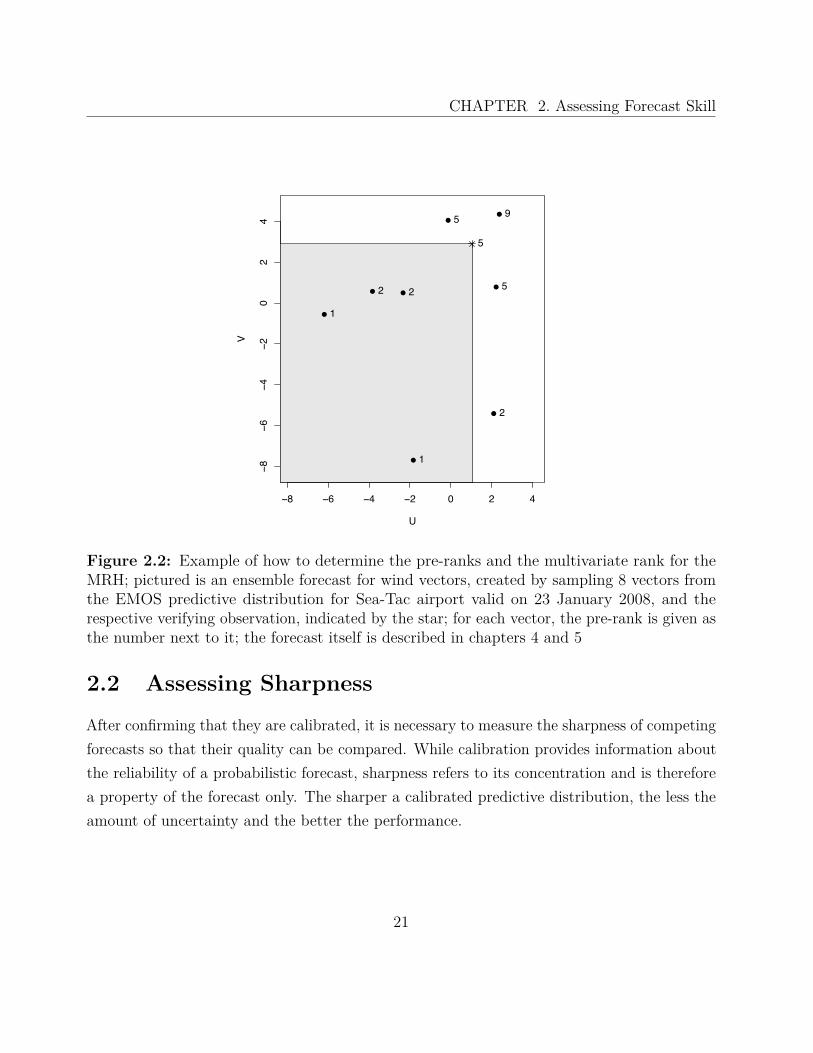
Figure 2.2 illustrates the process of determining first the pre-ranks and then the multivariateobservation rank. Four ensemble member forecasts lie to the lower left of the observationvector, i.e. are smaller in each of the vector components. The observed value therefore hasthe pre-rank 5, the same as two other ensemble members. The pre-ranks of five vectorsare smaller than that of the observation, so we sample the multivariate rank from the set{s< + 1, . . . , s< + s=} = {6, 7, 8}. In this case, r was chosen to be 6.
The multivariate rank histogram can be interpreted in the same manner as its univariatecounterpart. We will use this tool for assessing both ensemble and density forecasts, wherepredictive PDFs will be converted to discrete ensembles as described in Section 5.3.5. Thereliability index ∆ provides a measure for the deviation from uniformity, in the same manneras for the univariate histograms.
2.1.3 Marginal Calibration Diagram
Gneiting et al. (2007) refer to marginal calibration as the equality of forecast climate andobserved climate. If the forecast and the observation can be assumed compatible, theirrespective empirical distributions, aggregated over a number of cases in a steady state, shouldbe statistically consistent.
In the context of the thesis at hand, we check this property by a location-specific diagram.For each observational location, the empirical distributions of the raw ensemble, the EMOSmethod and the observations are plotted over the course of one calendar year. To representthe respective empirical distributions of the forecasts, for each date one random ensemblemember and one random vector from the EMOS predictive distribution are drawn.
We then say that a forecast is marginally calibrated if the pattern created by the windvector observations is approximately reproduced by the distribution of the forecast. The useof this so-called marginal calibration diagram can reveal forecast biases or dispersion errorsand especially address the possible influence of local terrain and surroundings.
20
CHAPTER 2. Assessing Forecast Skill
●
● ●
●
●
●
●
●
−8 −6 −4 −2 0 2 4
−8−6
−4−2
02
4
U
V
●
● ●
●
●
●
●
●
1
2 2
1
5
2
5
9
5
Figure 2.2: Example of how to determine the pre-ranks and the multivariate rank for theMRH; pictured is an ensemble forecast for wind vectors, created by sampling 8 vectors fromthe EMOS predictive distribution for Sea-Tac airport valid on 23 January 2008, and therespective verifying observation, indicated by the star; for each vector, the pre-rank is given asthe number next to it; the forecast itself is described in chapters 4 and 5
2.2 Assessing SharpnessAfter confirming that they are calibrated, it is necessary to measure the sharpness of competingforecasts so that their quality can be compared. While calibration provides information aboutthe reliability of a probabilistic forecast, sharpness refers to its concentration and is thereforea property of the forecast only. The sharper a calibrated predictive distribution, the less theamount of uncertainty and the better the performance.
21
CHAPTER 2. Assessing Forecast Skill
For univariate quantities, the sharpness measure of our choice is the standard deviationof both predictive PDFs and ensemble forecasts. In the two-dimensional case, we employ ageneralisation of the standard deviation, the determinant sharpness (DS)
DS = (det Σ)1/4
=�σ2
1σ22 ·
�1 − ρ2
��1/4,
with Σ =
σ21 ρ σ1σ2
ρ σ1σ2 σ22
being the variance-covariance matrix of the forecast. This tool is
also applicable to discrete ensembles, where the matrix is generated by the empirical variancesand correlation of the ensemble.
However, the determinant sharpness has a major disadvantage, which was brought up byJolliffe (2008). For nearly singular matrices, such as in the case of highly correlated variables, itbecomes very small, although the individual variances may be large. Therefore it is possible forsuch forecasts to seem sharper than those with smaller spread and correlation. This problemindeed arises in our case study and is discussed in Section 5.4.3.2.
2.3 Proper Scoring RulesAdditional to measuring the sharpness and calibration, the performance of a forecast can beevaluated by assigning a numerical score. For this we introduce a function s (P, x), where P isthe predictive distribution and x the observed vector or value. This function, called scoringrule, is negatively oriented and can be taken as a penalty. If we assume x to be drawn from adistribution Q, the expected value is written as s (P, Q). The idea of proper scoring rules andthe mathematical background are discussed in Gneiting and Raftery (2007).
Naturally, the intention of a forecaster should be to minimise the penalty by issuing thebest forecast he is able to make (Savage 1971; Bröcker and Smith 2007). Thus the scorebecomes the smallest when the true distribution is predicted. We say that a scoring rule isproper if
s (Q, Q) ≤ s (P, Q)
22

CHAPTER 2. Assessing Forecast Skill
holds for all P and Q, and strictly proper with equality if and only if P = Q. This propertyis very important for the assessment of our forecasts, meaning that a proper scoring ruleaddresses calibration and sharpness simultaneously by giving a measure for the overall skill(Winkler 1977, 1996).
In practical applications, the reported values are typically averaged over a period of timeor for a specific location. We note these mean scores as
Sn = 1n
n�
i=1s (Pi, xi) ,
where Pi and xi range over all forecast cases i = 1, . . . , n.
2.3.1 Univariate Forecasts
One of the scoring rules coming into use in the new EMOS method is the widely knownlogarithmic or ignorance score (Good 1952; Bernardo 1979). It can be applied to univariate aswell as multivariate density forecasts. For a predictive distribution P with density function p
and the observed vector or value x, the ignorance score is defined as
logs (P, x) = − log p (x) .
However, this proper scoring rule can assign infinite penalties, which poses problems inpractice. The so-called continuous ranked probability score (CRPS), proposed in Matheson andWinkler (1976), is more robust and also more versatile as it applies to density and ensembleforecasts. Gneiting and Raftery (2007) showed that the following two representations of theCRPS are equal, conditional on P having finite first moment:
crps (P, x) =∞
−∞
(F (x) − I {y ≥ x})2 dy (2.1)
= EP |X − x| − 12 EP |X − X �| . (2.2)
23
CHAPTER 2. Assessing Forecast Skill
Here, F denotes the cumulative distribution function of P , while X and X � are independentrandom variables with distribution P . In contrast to the ignorance score, the observation x
may only be a number rather than a multidimensional vector. The CRPS is reported in thesame unit as the observation which simplifies interpretability.
If we consider deterministic instead of probabilistic forecasts, we are interested in thepredictive skill of an ensemble or a predictive distribution when issuing a point forecast µ.According to Gneiting (2011), the most effective way of producing point forecasts is to specifya scoring rule in advance and then choose the optimal point predictor for the scoring rule athand, i.e. the Bayes rule. In the situation above, P can be taken as a point measure δµ andthe CRPS reduces to the absolute error
ae (P, x) = |µ − x| .
The respective Bayes rule for the absolute error is the median of the predictive distribution,medP . We will use the mean absolute error (MAE) of the forecast median and the mean CRPSmainly for testing the skill of the new EMOS method for wind vectors when transformed intowind speed forecasts (Section 5.5).
2.3.2 Multivariate Forecasts
The direct generalisation of the CRPS to multiple dimensions is called the energy score (ES),introduced by Gneiting and Raftery (2007). It derives from the kernel score representation(2.2) and uses the Euclidean norm �·� instead of the absolute value:
es (P, x) = EP �X − x� − 12 EP �X − X�� ,
where X and X� are independent random vectors distributed with P and x is the observationvector.
For ensemble forecasts, where the predictive distribution Pens places a point mass of 1M on
the ensemble members x1, . . . , xM ∈ R2, the energy score can easily be evaluated as
24

CHAPTER 2. Assessing Forecast Skill
es (Pens, x) = 1M
M�
j=1�xj − x� − 1
2M2
M�
i=1
M�
j=1�xi − xj� .
However, for most densities this proper scoring rule is not straightforward to compute. Aswe use bivariate normal distributions, a Monte Carlo approximation can replace the usualform of the energy score, reducing the computational effort notably. The energy score thenbecomes
�es (P, x) = 1k
k�
i=1�xi − x� − 1
2 (k − 1)
k−1�
i=1�xi − xi+1� ,
where x1, . . . , xk is a simple random sample of size k = 10, 000, drawn from the predictivedistribution P .
Again, deterministic forecasts can also be assessed by this scoring rule. As in the case ofthe CRPS, we set P to be the point measure δµ. The resulting score is called the Euclideanerror (EE) and is the generalisation of the absolute error:
ee (P, x) = �µ − x� .
As point forecast µ, we choose the appropriate Bayes rule, the spatial median medP . Consid-ering an ensemble forecast, it is defined as the vector that minimises the sum of the Euclideandistances to the ensemble members,
M�
i=1�medP − xi� .
This vector can only be determined numerically, e.g. using the algorithm described in Vardiand Zhang (2000) and implemented in the R package ICSNP.
In this chapter different tools for the assessment of both ensemble and density forecasts wereintroduced. These tools will be used in Chapter 5 to analyse and compare the performanceof several competing forecasting and postprocessing techniques. The univariate and themultivariate rank histograms and the PIT histogram help us to test forecasts for calibration,while the marginal calibration diagram unmasks local biases and dispersion errors. As to the
25

CHAPTER 2. Assessing Forecast Skill
sharpness, the determinant sharpness provides a way to quantify the spread of multivariatedistributions. Proper scoring rules are able to assess calibration and sharpness simultaneouslyand therefore can be employed for the parameter estimation. The conventional EMOS methodfor univariate weather quantities, for instance, described in the following chapter, relies onminimum CRPS estimation.
26
Chapter 3
EMOS for Univariate WeatherQuantities
In Chapter 1, we already mentioned the well-established statistical postprocessing methodEMOS, also called non-homogeneous Gaussian regression, and stated that such techniques canimprove the quality and accuracy of weather forecasts significantly. EMOS was first proposedby Gneiting et al. (2005) and then developed further in Thorarinsdottir and Gneiting (2010)and Thorarinsdottir and Johnson (2011). Our goal is to find a two-dimensional extensionwhich applies to wind vectors by capturing the essential properties of the one-dimensionalvariant. The idea and concept behind EMOS is the subject of this chapter.
3.1 General IdeaStandard model output statistics (MOS) techniques profit from determining a statisticalrelationship between the predictive weather quantity and the output variables of a numericalmodel (Glahn and Lowry 1972; Wilks 1995). For instance, the prediction of wind speed cancorrelate strongly with the wind vector forecast or with past wind speed observations. Theseare then combined as predictors in a multiple linear regression equation.
EMOS is a form of MOS or multiple linear regression; here, the ensemble members functionas predictors. By fitting a normal distribution with the regression estimate as predictive
27

CHAPTER 3. EMOS for Univariate Weather Quantities
mean, and the mean squared prediction error of the training data as predictive variance, afull probability distribution can be gained from a regression equation. This straightforwardway, however, does not take account of a potential relationship between ensemble spreadand forecast skill (Whitaker and Loughe 1998). Therefore, the EMOS method models thepredictive variance as an affine function of the ensemble variance.
This simple concept addresses forecast biases and dispersion errors on one hand and benefitsfrom the skill of the underlying numerical models on the other. It therefore combines statisticaland numerical weather prediction, while being very parsimonious and easy to implement.
3.2 Standard EMOSIn this section, we discuss EMOS as it was originally described by Gneiting et al. (2005). Itapplies to any weather quantity Y , whose distribution, conditional on the ensemble memberforecasts X1, . . . , XM , can be modelled with a normal distribution; such quantities are surfacetemperature, sea level pressure, or wind vector components (see Section 5.3.3).
For the predictive mean, the authors suggest a linear regression equation with the ensemblemembers as predictors and the observation Y as predictand,
Y = a + b1X1 + . . . + bMXM + ε.
The error term ε has distribution N (0, c + d S�), where S� = 1M
�Mi=1
�Xi − X
�2is the
empirical variance of the ensemble and X = 1M
�Mi=1 Xi the ensemble mean. The variance
term corrects the underdispersion of the ensemble, while taking account of the spread-errorcorrelation. Thus, the full predictive distribution for Y is denoted as
Y | X1, . . . , XM ∼ N�a + b1X1 + . . . + bMXM , c + d S2
�.
The coefficients b1, . . . , bM can be interpreted as the performance of the individual ensemblemember models over the training period, relative to the other members. Additionally, highlycorrelated ensemble members can be identified, as typically the most skillful of them receivesa substantial coefficient estimate, while the estimates of the others are nearly zero.
28

CHAPTER 3. EMOS for Univariate Weather Quantities
The spread parameters c and d reflect the relationship between the ensemble spread andthe forecast error in the training data. If there is a significant correlation between these two,d tends to be larger and c smaller. On the other hand, when there is no information to begained by the ensemble variance, d will be negligibly small and c very large.
For estimating the parameters a, b1, . . . , bM , c, and d, Gneiting et al. (2005) employminimum score or minimum contrast estimation: They choose a proper scoring rule, write thescore for the training data as a function of the parameters to estimate and numerically minimisethis function. The results can be interpreted as the coefficients for which this particular scorewould have been minimal, when summed up over the training data. Picking a proper scoringrule ensures that calibration and sharpness are addressed simultaneously (Section 2.3).
In this context, the CRPS proves suitable, and Gneiting and Raftery (2007) have shownthat it is more robust than e.g. the logarithmic score. Therefore, this estimation method isreferred to as minimum CRPS estimation. Modelling Y with a normal distribution has theadvantage of simplifying the computing of the CRPS, as a closed form can be obtained usingrepeated partial integration:
crps�N
�µ, σ2
�, y
�= σ
�y − µ
σ
�2 Φ
�y − µ
σ
�− 1
�+ 2 ϕ
�y − µ
σ
�− 1√
π
�
,
where Φ (·) and ϕ (·) denote the CDF and the PDF of the standard normal distribution,respectively.
The variance coefficients c and d should be non-negative to make certain that the varianceis positive and we have a valid probability distribution. Gneiting et al. (2005) set d = δ2,optimise the CRPS over δ and in this way enforce the non-negativity; here, it is not an issuefor the parameter c, but generally one can proceed in the same manner as for d.
When expressing the CRPS in terms of the parameters, the average score over all k pairsof forecasts and observations contained in the training data set is noted,
Γ (a; b1, . . . , bM ; c; δ) = 1k
k�
i=1
�c + δ2 S2
i
�
Mi
�2 Φ (Mi) − 1
�+ 2 ϕ (Mi) − 1√
π
�
,
where
29

CHAPTER 3. EMOS for Univariate Weather Quantities
Mi = Yi − (a + b1Xi1 + . . . bMXiM)�
c + δ2 S2i
is the standardised forecast error for the ith forecast in the training data set. Using theBroyden-Fletcher-Goldfarb-Shanno algorithm, as it is implemented in the R function optim,the authors determine the minimum of the CRPS numerically. Reaching a global minimumcan not be ensured, so the initial values have to be chosen carefully. The best way to do so isto take starting values based on past experiences, e.g. the estimated parameters from the daybefore.
3.2.1 EMOS+
In the previously described method for estimating the EMOS parameters, no constraints wereassumed on the ensemble member coefficients b1, . . . , bM . However, in the context of ensembleforecasts and statistical postprocessing, it is hard to explain negative values, as these parameterscan be interpreted as weights, reflecting the relative usefulness of the particular ensemblemember model. Such negative coefficients might be caused by highly correlated ensembleforecasts, e.g. because the initial and boundary conditions for the underlying numerical modelsare provided by the same operational weather centre.
To solve this issue, Gneiting et al. (2005) proposed an extended technique, called EMOS+,producing only non-negative EMOS weights. At first, the usual estimation is executed, withno constraint on b1, . . . , bM . Then all ensemble member forecasts with negative coefficients areremoved from the training data and their respective coefficients are set to zero. The ensemblemean X and variance S2 need to be recomputed, both for the training data and the forecast,using only the remaining ensemble members. This process is iterated until there are onlynon-negative regression parameters left.
The described approach can easily be interpreted as a form of model selection, wherethe most useful of the ensemble member models are chosen. Highly correlated models areoften eliminated, and only the most skillful of them is left in the regression equation. Usually,EMOS+ yields similar results in comparison to EMOS, but improves interpretability.
30
CHAPTER 3. EMOS for Univariate Weather Quantities
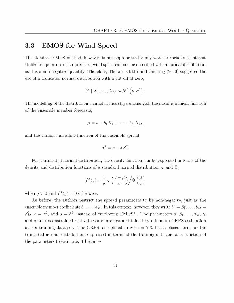
3.3 EMOS for Wind SpeedThe standard EMOS method, however, is not appropriate for any weather variable of interest.Unlike temperature or air pressure, wind speed can not be described with a normal distribution,as it is a non-negative quantity. Therefore, Thorarinsdottir and Gneiting (2010) suggested theuse of a truncated normal distribution with a cut-off at zero,
Y | X1, . . . , XM ∼ N 0�µ, σ2
�.
The modelling of the distribution characteristics stays unchanged, the mean is a linear functionof the ensemble member forecasts,
µ = a + b1X1 + . . . + bMXM ,
and the variance an affine function of the ensemble spread,
σ2 = c + d S2.
For a truncated normal distribution, the density function can be expressed in terms of thedensity and distribution functions of a standard normal distribution, ϕ and Φ:
f 0 (y) = 1σ
ϕ�
y − µ
σ
��Φ
�µ
σ
�
when y > 0 and f 0 (y) = 0 otherwise.As before, the authors restrict the spread parameters to be non-negative, just as the
ensemble member coefficients b1, . . . , bM . In this context, however, they write b1 = β21 , . . . , bM =
β2M , c = γ2, and d = δ2, instead of employing EMOS+. The parameters a, β1, . . . , βM , γ,
and δ are unconstrained real values and are again obtained by minimum CRPS estimationover a training data set. The CRPS, as defined in Section 2.3, has a closed form for thetruncated normal distribution; expressed in terms of the training data and as a function ofthe parameters to estimate, it becomes
31
CHAPTER 3. EMOS for Univariate Weather Quantities
Γ (a; β1, . . . , βM ; γ; δ) = 1k
k�
i=1Φ (Ni)−2
�γ2 + δ2S2
i
�
Mi Φ (Ni)�2 Φ (Mi) + Φ (Ni) − 2
�
+ 2 ϕ (Mi) Φ (Ni) − 1√π
Φ�√
2 Ni
��
,
where
Mi = yi − (a + β21Xi1 + . . . + β2
MXiM)√
γ2 + δ2S2and Ni = a + β2
1Xi1 + . . . + β2MXiM√
γ2 + δ2S2.
Once more, the actual numerical optimisation, i.e. finding the parameter values which minimisethe CRPS for the training data, rests on the Broyden-Fletcher-Goldfarb-Shanno algorithm.The initial values for this algorithm are the estimated parameters of the previous day, toenhance the probability of finding a global minimum.
3.4 EMOS for Wind GustThe forecasting of wind gust is challenging, as it is typically not an output of numericalweather prediction models. There seems to be a direct relation to wind speed, though, namelythrough a gust factor τ , the ratio between the maximum gust speed and the sustained windspeed. Thorarinsdottir and Johnson (2011) developed a forecasting method depending on thepreviously described EMOS method for wind speed. It consists of three components whichhave to be predicted:
1. Daily maximum wind speed:For the daily maximum wind speed, the EMOS model defined above is employed topostprocess the ensemble forecasts and obtain a full predictive distribution. In a first step,the parameters a, b1, . . . , bM , c, and d are estimated with minimum CRPS estimation.
2. Probability of gust:The gust speed Z can be assumed to have a multiplicative relationship to the wind speedY ,
Z = τY, τ ≥ 1.
32

CHAPTER 3. EMOS for Univariate Weather Quantities
Then the conditional predictive distribution for Z becomes
Z | X1, . . . , XM ∼ N 0�τµ, (τσ)2�
,
with µ and σ2 denoting the mean and variance estimates for the wind speed.In the context of the article, using observations from the Automated Surface ObservingSystem (ASOS) network (National Weather Service 1998), gust is observed if the gustspeed, determined under certain conditions, is at least 14 knots. The authors introducetwo separate gust factors, τ1 for the probability of gust and τ2 for the conditional gustspeed forecast. Thus, in the former case, they draw on the predictive distribution for Z
and express this probability in terms of τ1:
P (Z ≥ 14 | X1, . . . , XM) =�1 − Φ
�14 − τ1µ
τ1σ
���Φ
�µ
σ
�.
This parameter can also be estimated by minimum score estimation, using the Brier skillscore for categorical events (e.g. Gneiting and Raftery 2007). The task is to find thevalue for τ1 which minimises
Γ (τ1) = 1k
k�
i=1
��1 − Φ
�14 − τ1µ
τ1σi
��Φ
�µi
σi
�−1− I {Zi observed }
�2
over the training set, where I {Zi observed } is 1 if gust is observed for the ith forecastcase (according to the definition in National Weather Service (1998)), and zero otherwise.
3. Daily maximum gust speed, conditional on gust being observed:Subsequently, the gust speed, conditional on gust being observed, needs to be addressed.Its predictive distribution can be modelled employing a truncated normal distribution,as with the wind speed, however now the cut-off is at 14. With the second gust factorτ2, the predictive density becomes
f 14 (z) =� 1τ2σ
ϕ�
z − τ2µ
τ2σ
����1 − Φ
�14 − τ2µ
τ2σ
��
33

CHAPTER 3. EMOS for Univariate Weather Quantities
for z ≥ 14 and f 14 (z) = 0 otherwise. Following the usual technique, CRPS minimisationis applied over training data to find the optimal value for τ2. For this distribution, theCRPS can be determined as
crps�N 14 (τ2µ, τ2σ) , z
�=
τ2σ λ (τ2µ, τ2σ)−2�
z − τ2µ
τ2σλ (τ2µ, τ2σ)
�2 Φ
�z − τ2µ
τ2σ
�+ λ (τ2µ, τ2σ) − 2
�
+2 ϕ�
z − τ2µ
τ2σ
�λ (τ2µ, τ2σ) − 1√
π
�1 − Φ
�√2 14 − τ2µ
τ2σ
���
,
where λ (a, b) = 1 − Φ�
14−ab
�and z ≥ 14. Here, the observations z are the gust speed
observations, and the parameters µ and σ originate from the estimation of the windspeed forecast.
All numerical optimisation is done using the Broyden-Fletcher-Goldfarb-Shanno algorithm.With this method, it is possible to obtain full predictive densities for a weather variable whichnormally is not included in numerical weather prediction models. It can, however, also beapplied as a statistical postprocessing method for ensemble forecasts of gust speed.
The EMOS approach was developed to produce calibrated and sharp predictive distributionsfrom underdispersed discrete ensemble forecasts. It has proved to be a very versatile method,being applicable to several weather variables such as temperature, air pressure, wind speedand wind gust. To adapt to local circumstances, the normal distribution can be substitutedby a more adequate distribution, e.g. the Student’s t distribution.
In the next chapter we will propose a bivariate variant that incorporates the correlationbetween two components into the model. More information about the different univariateEMOS methods, as well as results in form of case studies, can be found in the respectivearticles.
34
Chapter 4
Extending EMOS to Wind VectorForecasts
In this chapter, a new method based on the conventional univariate EMOS postprocessingtechnique is designed, where ensemble forecasts of two weather quantities are addressedjointly. EMOS is a very useful and easy to implement way to improve the performance ofwind speed forecasts (Thorarinsdottir and Gneiting 2010); there is also a variant of BayesianModel Averaging for the direction of surface wind, developed by Bao et al. (2010). It isquite conceivable that especially EMOS can be applied to the latitudinal and longitudinalwind components individually. In this case, however, we do not make use of dependenciesbetween the components. Therefore, we will introduce a method that employs a bivariatejoint distribution and thus takes account of the correlation structure.
At first we have to become accustomed to the different properties of wind vectors, beforewe move on to examining some data and decide which bivariate distribution is best used. Inthe then following sections, it will be established how the model characteristics can be writtenin terms of the ensemble forecasts. Compared to the univariate EMOS technique, we will makesome changes to the process of parameter estimation in that we will split it in three partsand use historic data to estimate the correlation structure. Still, the essential ideas stay thesame: EMOS for wind vectors is based on linear regression, takes account of the spread-errorrelationship contained in the ensemble and produces calibrated and sharp forecasts.
35

CHAPTER 4. Extending EMOS to Wind Vector Forecasts
4.1 Properties of Wind VectorsBefore we can define a model for the bivariate predictive distribution of wind vectors, wehave to take a look at their properties and how they are measured. For this, consider Figure4.1, where the green arrow represents the surface wind vector. It is the sum of a zonal and ameridional component, respectively named U and V . They therefore correspond to the partsof the wind flowing in west/east and north/south direction. For the creation of weather maps,the vectors are often illustrated as wind barbs, using shafts of a fixed length with differentkinds of barbs and flags for different wind speeds.
Wind vectors indicate wind speed and wind direction simultaneously through the lengthand the angle of the vector. While the angle θ is measured in degrees (clockwise from north),the wind is always named after the direction where it originates from, so for example an angleof 90° means easterly wind, 225° southwesterly wind and so on. The wind speed w can becomputed from the wind components U and V , using the euclidean norm:
w =√
U2 + V 2.
Surface wind is typically quantified in meters per second or in knots, where 1 knotapproximately equals 0.514 m/s. Our new method will be applied to instantaneous 10 m wind,which means that the wind observations are averaged over the last 2 minutes of the hour andmeasured at 10 m above ground (see also Thorarinsdottir and Gneiting (2010), where thedaily maximum wind speed was used). In practice, instead of the wind components, the winddirection θ and wind speed w are observed and then transformed into vectors.
Next, we will develop a two-dimensional model for the joint distribution of U and V .Our goal is to take advantage of a possible correlation between the two components and socapture dependencies and account for local terrain characteristics. We begin with a short dataanalysis where we use ensemble forecasts from the UWME ensemble for the Pacific Northwestof the USA and parts of Canada, as well as the corresponding verifying observations. Furtherinformation on the data can be found in Section 5.1.
36

CHAPTER 4. Extending EMOS to Wind Vector Forecasts
Figure 4.1: Wind vector, wind components U and V and wind direction θ
4.2 EMOS for Wind VectorsTo modify the conventional EMOS postprocessing method so that it can be applied to windvectors, we begin by finding a bivariate distribution which represents the empirical distributionof wind vector observations as closely as possible and which is easy to work with. Again, welook at the conditional distribution of the observations given the forecasts.
In the two-dimensional case, we at first restrict the following analysis to the ensemble meanforecast, as compared to the full ensemble in the univariate case. This approach naturallyapplies only to ensembles with exchangeable members, but is done here because of simplicityreasons. Exchangeable members are ensemble member forecasts that only differ in randomperturbations, and are therefore indistinguishable. The UWME ensemble does not consist ofexchangeable members, but we will see that the performance of the new method is not verysensitive to the use of the ensemble mean only. On the contrary, it reduces the amount ofparameters to estimate and helps simplifying the model.
37

CHAPTER 4. Extending EMOS to Wind Vector Forecasts
Figure 4.2: The R2 plane, divided into nine sections
4.2.1 Data Analysis
In the univariate EMOS method, it was established that the predictive distribution of theweather quantity of interest, conditional on the ensemble forecasts, can be modeled with anormal distribution. For the two-dimensional wind vectors, we hope to employ a bivariatenormal distribution, but we first have to test if this conjecture is justified.
To examine the wind vector distribution empirically, we use data provided by the UWME,consisting of the ensemble forecasts and the corresponding verifying observations. For thispurpose, we divide the plane of real numbers into nine sections (according to Figure 4.2) and,for each section, we plot the observations conditional on the corresponding ensemble meanforecast falling into this section. So, for the predictive distribution to be bivariate normal,these scatterplots should roughly have the shape of a circle or an ellipse, depending on thecorrelation between the vector components. To create these plots, data from the years 2007and 2008 at 79 stations is used. All values are given in m/s.
38

CHAPTER 4. Extending EMOS to Wind Vector Forecasts
−20 −10 0 10 20
−20
−10
010
20
Section 9
U
V ●
●
●
●
●
●
●
●
●
●
● ●
●
●
●
●●
●
●
●
●
●
●
●
●
●
●
●
●
●
●
●
●●
●
●
●
●●
●
●
●●●
●●
●
●
●
●●
●
●
●
●
●
●
●●
●
●
●
●
●
●
●●
●
●
●
●
●
●
●
●
●
●
●
●
●
●
●
●
●
●
●
●
●
●
●
●
●●
●●
●
●
●
●
●
●
●
●
●
●
●
●
●
●●
●
●
●
●
●●
●
●●
●
●
●
●
●
●
●
●
●
●
●
●
●
●
●
●●
●●
●
●
●
●
●
●
●●●
●
●
●
●
●
●
●
●
●
●
●
●
● ●
●
●
●
●
● ●
●
●
●
●●
●
●
●
●
●
●
●
●
●
●
●
●
●
●
●
●
●
●
●
●
●
●
●
●●
●
●
●
●
●●
●
●
●●
●
●
●
●●
●
●
●
●
●●
●
●
●
●
●
●
●●
●
●
●
●
●
●
●
●
●
●
●
●
●
●
●
●
●●
●
●
●● ●
●
●
●
●●
●
●
●
●
●
●
●●
●
●
●
●
●
●
●
●
●
●
●●
●
●
●●
●
●
●
●
●
●
●
●
●
●
●●
●
●
●
●
●
●
●
●
●● ●
●
●●●
●
●
●
●
●
●●
●●●
●
●
●●
●●
●
●
●●
●
●
●
●
●
●
●
●●
●
●
● ●
●
●
●
●
●
●
●
●●●
●
●●
●
●
●
●
●●●
●
●●●
●
●
●
●
●
● ●●
●
●
●
●●
●
●
●●
●
●
●●
●
●
●
●
●
●
●
●
●
●
●
●
●
●●●
●
●●●
●
●
●
●●
●●
●
●
●
●
●
●
●
●
●
●
●
●
●
●
●
●
●
●
●
●
●
●
●
●
●
● ●●
●
●
●
●
●
●
●
●
●
●
●
●
●
●
●
●
●●
●●
●●
●
●
●
●
●
●
●
●
●
●
●
● ●●
●
● ●
●●
●
●
●
●
●
●
●●
●
●
●
●
●
●
●
●●
●●
●
●
●
●
● ● ●
●
●
●
●
●
●
●
●
●
●
●
●●
●
●
●
●
●
●
●
●
●
●
●●
●
●
●
●
●●
●●
●
●
●●
●
●
●●
●
●
●●
●
●
●
●
●
●
●●
●
●
●●●
●
●●●
●
●●●
●
●
●
●
●●
●
●
●
●
●
●
●
●
●
●
●
●
●
●
●
●
●
●
●
●
●
●
●
●
●
●
●●
●
●
●
●
●
●
●
●
●
●
●
●
●
●
●
●
●
●●
●●
●
●
●
●
●
●
●
●
●
●
●
●●
●
●
●
●
●
●
●
●
●●
●
●●
●●
●
●
●●
●
●
●
●
●
●
●
●
●
●
●
●
●
●●
●●
●
●●
●
●●
●
●●
●
●
●
●
●
●
●
●
●
●
●
●
●
●●
●
●
●
●
●
●●
●●
● ●
●
●●
●
●
●
●
●
●
●
●
●
●
●
●
●
●
●
●
●
●
●
●
●
●
●
●
●
●
●
●
●
●
●
●
●
●
●
●
●
● ●
●
●
●
●
●
●●
●
●
●
●
●
●
●
●
●
●
●
●
●
●
●
●●
●
●
●
●
●
●
●
●
●
●
●●
●
●
●
●
●●
●
●
●
●
●
●
●●
●
●
●
●
●
●
●
●
●
●
●
●
●
●
●●●
●
●
●
●
●
●●
●
●
●
●
●●
●●
●
●
●
●
●
●
●●●
●●
●
●
●
●
●●
●
●
●
●
●
●
●
●
●
●
●
● ●
●
●
●
●
●
●●●
●
●
●
●
●
●
●
●
●
●
●
●
●
●
●
●
●
●
●
●●
●
●
●
●
●
●
●
●
●
●
●
●
●
●
●●●
●
●
●
●
●
●
●
●
●
●
●
●
●
●
●
●
●
●
●
● ●
●
●
●
●
●
●
●
●
●
●
●
●
●
●
●
●
●
●
●
●
●
●
●
●
●
●
●
●
●
●●
●
●
●
● ●
●
●●
●
●
●
●
●
●
●
●
●
●
●
●
●
●●
●●
●
●
●
●
●
●●
●
●
●
●
●
●
●
●
●●
●
●
●
●
●
●
●
●
●
●
●
●
●
●
●●
●●
●
●●●
●
●
●
●
●
●
●●
●
●
●●
●
●
●
● ●
●
●
●●
●
●
●●
●
●
●
●
●
●
●
● ●
●
●
●
●●
●●
●
●
●
●
●
●
●
●
●
●
●
●
●
●
●●
●
●
●
●
●
●
●
●
●
●
●
●
●
●
●
●●
●
●●
●
●
●
●
●
●
●
●
●
●
●
●
●
●
●●
●
●
●●
●
●
●
●
●
●●
●●
●
●
●
●
●
●●
●
●
●
●
●
●
●
●
● ●●
●●●
●
●
●
●
●
●
●
●
●
●
●
●
●
●
●●
●
●
●
●
●
●
●●●
●
●
●
●
●
●
●
●
●
●
●
●
●
●
●
●
●
●●
●
●
●
●
●
●
●
●
●
●
●
●
●
●
●
●
●
●
●
●
●
●
●
●
●
●
●
●
●
●
●
●
●
●
●
●
●●●
●
●
●
●●
●
●
●
●
●
●
●
●
●●●
●●
●
●
●
●●
●
●
●
●●
●
●
●
●●
● ●
●
●
●
●
●
●
●
●
● ●
●
●
●
●
●
●●
●
●
●
●
●
●
●
●
●
●●
●
●
●
●
●
●
●
●
●
●●
●
●
●
●
●
●
●
●
●
●
●
●
●
●
●
●
●
●●
●
● ●●
●
●
●
●
●
●
●
●
●
●
●●
●
●
●
●
● ●●●
●
●
●
●
●
●
●
●
●
●
●
●
●
●
●
●
●
●
●
●
●
●
●
●
●
●
●
●●
●
●
●
●
●
●
●
●
●
●
●
●
●
●
●
●
●
●
●
●
●
●
●
●
●
●●
●
●
●
●
●
●
●●
●●
●●
●
●
●
●
●
●
●
●
●●
●
●
●
●●
●●
●
●
●
●
●
●
●
●●
●
●
●
●
●
●
●
●
●
●
●●
●
●●
●
●
●
●
●
●
●●
●
●
●
●
●
●
●
●●
●●
●●
●
●
●
●
●●
●
●
●
●
●
●
●
●●
●●●
●
●
●
● ●
●
●
●
●
●
●
●
●●●
●
●●
●
●
●
●
●
●●
●
●
●
●
●
●●
●
●
●
●
●
●
●
●
●
●
●
●
●
●
●
●
●
●
●
●
●
●
●
●●
●
●
●
● ●
●
●
●
●
●
●
●
●
●
●
●
●
●
●
●
● ●●
●
●
●●
●●●
●
●
●
●
●●
●
●
●
●
●
●
●
●
●●
●
●
●
●
●
●
●
●
●
●
●●
●●●
●
●
●
●
●
●
●
●
●●
●
●
●
●
●
●
●
●
●●
●
●
●
●
●
●
●
●●
●
●
●
●
●
●
●
●
●
●
●
● ●
●
●
●
●
●
●●
●
●
●
●
●
● ●●
●
●
●
●
●
●●
●●
● ●
●
●
●
●
●
●
●●
●
●
●
● ●
●●
●●
●
●
●
●
●●
●
●
●
●
●
●
●
●●
●
●
●
●
●
● ●
●●
●
●
● ●
●
●
●
●
●
●
●
●
●
●
●
●●
●
●
●
●
●
●
●
●
●
●
●
●
●
●
●
●●
●●
●
●
●
●
●
●
●
●
●
●
●
●
●
●
●
●
●
●●
●
●
●
●
●
●
●
●●
●
●
−20 −10 0 10 20
−20
−10
010
20
Section 2
U
V
●
●
●
●
●
●●
●
●
●
●
●
●
●
●
●
●
●
●
●
●
●
●
●
●
●
●
●●
●
●
●
●
●
●
●
●
●
●
●
●
●
●
●
●
●
●
●
●●
●
●
●
●
●●
●
●
●
●
●●
●●
●
●
●
●
●
●
●
●
●
●
●●
●
●
●
●
●
●
●
●
●
●
●
●
●
●
●●
●
●●
●
●
●
●
●
●
●
●
●
●
●
●
●
●
●
●
●
●
●
●
●
● ●●
●
●●
●
●
●
●
●
●
●
●
● ●
●●
●
●
●
●
●●
● ●
●
●
●
●●
●●
●
●●
●
●
●
●●
●
●●
●
●
●
●
●
●
●
●●
●●
●
●●
●
●
●
●
●
●●
●
●
●
●
●
●
●
●
●
●
●
●
●
●
●
●
●
●
●
●
●
●
●
●
●●
●
●
●
●
●
●
●
●
●●
●
●
●
●
●
●
●
●●
●
●
●
●
●
●
●
●●
●●
●
●
●●
●
●
● ●
●●
●
●
●
●
●
● ●
●●
●
●
●
●●
●
●
●
●
●
● ●●
●●
●
●
●
●
●
●
●
●
●
●
●●
●
●
●
●●
●
●
●
●
●
●
●
●
●
●
●
●
●
●
●
●
●
●
●●
●
●
●
●●
●
●
●
●●
●●
●
●●●●
●
●
●
●
●
●
●
●
●
●
●
●
●
●
●
●
●
●
●
●●
●
●
●
●
●●●●
●
●
●
●●
●
●
●
●●
●
●
●
●
●
●
●
●
●
●
●
●
●
●
●●
●
●●
●
●
●
●
●
●
●
●
●
●
●
●
●
●
●●
●●
●●
●
●
●
●
●
●
●
●
●
●
●
● ●
●
●
●
●
●
●●
●
●
●
●
●
●
●
●
●
●
●
●
●
●
●
●
●
●
●
●
● ●
●
●
●
●●
●
●
● ●
●●
●
●
●
●
●
●
●
●
●
●
●
●
●
●
●
●
●
●
●
●
●●
●
●
●
●
●
●
●
●
●
●●
●
●
●
●
●
●
●
●
●
●
●
●
●
●
●●●
●
●
●
●
●●● ●●
●
●
●
●
●
●●
●●
●
●
●
●
●
●
●●
●
●
●
●
●
●
●
●
●●
●
●
●
●
●
●
●
●
●
●
●
●●
●
●
●
●●
●
● ●
●
●
●
●
●
●
●
●
●
●
●
●
●
●
●
●
●
●
●
●
●
●
●
●●
●●
●
●
●
●
●●
●
●
●
●●
●
●
●
●
●
●
●
●
●
●
●
●
●
●
●
●
●
●●
●
●
●
●
●
●
●
●
●
●
●●
●
●
●
●
●
●
●
●
●
● ●
●
●
●
●
●
●
●
●
●
●
●
●
●
●
●
●
●●
●
●
●
●●
●
●
●
●
●
● ●
●
●●
●
●●
●
●●
●
●
●●●
● ●●●
●
●
●
●
●●
●
●
●
●
●
●
●
●
●
●
●●●
●
●
●
●
●
●
●
●●
●●
●
●
●
●
●●
●
●
●
●
●
●●
●
●
●
●●
●●●
●
●
●
●
●●
●
●
●
●
●
●●
●
●
●
●
●
●●
●
●●
●
●
●
●
●
●
●
●
●
●●
●
●
●
●●
●●
●
●
●
●
●
● ●
●●
●
●
●
●●
●
●
●
●
●
●
●●
●
●
●
●● ●
●
●
●
●
●
●
●
●●●
●
●
●
●
●
●
●
●
●
●
●
●
●
●
●
●●
●
●
●
●
●
●
●
●
●
●
●
●
●
●
●
●
●
●
●
●
●
●
●●● ●
●
●
●
●
●●
●
●
●●
●
●
●● ●
●●
●
●●●
●●
●
●
●
●
●●
●
●
● ●
●
●
●
●
●
●●
●
●
●
●
●
●
●
●
●
●
●
●
●
●
●●
●
● ●
●
●
●
●
●
●
● ●
●
●
●
●
●
●
●
●
●
●
●●
●
●
●
●
●
●
●
●
●●
●
●●
●
●
●
●
●
●●
●
●●●
●
●
●
●
●
●
●
●
●
●
●
●
●
●
●●
●
●●
●
●
●
●
●
●
●
●●
●
●
●●
●
●
●
●
●
●
●
●
●
●
●
●
●
●
●
●
●
●
●●
●●
●●
●
●
●
●●
●
●
●
●
●
●
●
●
●
●
●●
●
●
●
● ●
●
●
●
●
●
●
●
●
●●
●
●
●●
●
●
●
●
●●
●
●
●
●
●
●
●
●
●
●
●
●
●●
●●
●
●
●
●
●
●
●
●
●
●
●
●
●
●
●
●
●
●
●
●
●
●
●
●
●
●
●
●
●
●
●
●
●
●
●
●
●
●
●●●
●
●
●
●
●
●
●
● ●
● ●
●
●
●
●
●
●
●
●
●
●
●
●
●
●
●
●
●
●
●
●
●
●●
●
●●
●
●
●
●
●
●
●●
●●
●
●
●
●●●
●●
●
●
●
●
●
●
●
●
●
●●
●
●
●
●
●●
●
●
●
●
● ●
●
●
●
●●
●
●
●
●
●●
●●
●●
●
● ●
●
●
●
●
●
●
●
●
●
●
●
●
●
●
●
●●
●
●●
●
●
●
●
●
●
●
●
●●
●
●
●
●
●
●
●
●
●
●●
●
●
●
●
●
●
●
●
●
●●
●
●
●●
●
●
●
●
●
●
●
●
●
●
●
●
●
●
●
●
●
●
●●
●
●
●
●
●
●
●
●
●●
●
●
●
●
●
●
●
●●
●
●
●●
●
●
●
●
●
●
●
●
●
●
●
●
●
●
●
●
● ●
●
●
●
●
●
●
●
●
●
●
●
●
●
●
●
●
●
●
●
●●
●
●●
●
●
●
●
● ●
●
●
●
●
●
●
●
●
●
● ●
●●
●
●●
●
●
●
●
●●
●
●●●
●
●
●
●
●
●
●
●
●
●
●
●
●
●
●●
●
●
●
●
●
●
●
●
●
●
●
●
●
●
●
●
●
●
●● ●
●
●
●
●
●
●●
●
●
●
●●
●
●
●●
●
●
●
●
●
●●
●
●
●
●
●
●
●●
●
●●
●
●●
●
●
●
●
●
●
●
●
●
●
●
●●
●
●
●
●
●
●
●
●
●
●
●
●
●
●●
●
●
●
●
●
●
●
●
●
●
●
●
●
●
●
●
●
●
●
●
●
●
●
●
●
●
●●
●
●
●
●
●
●
●
●
●
●
●
● ●
●
●
●
●
●●
●●
●
●
●
●
●●
●●
●
●
●
●
●
●
●●
●●
●●
●
●
●
●
●
●
●
●
●
●
●
●●
●
●
●
●
●
●
●
●
●
●
●
●
●
●
●●
● ●
●
●
●
●
●
●
●
●
●
●
●
●
●●
●
● ●
●
●
●●
●
●
●
●
●
●
●
●
●●
●
●
● ●
●●
●
●
●
●
●
● ●●
●
●
●
●
●
●
●●
●
●
●
●
●
●
●
●
●
●
●
●
●
●
●
●●
●
●
●
●
●
●
●
●●
●
●
●
●
●
●
●
●
●
●
●
●
●
●
●
●●
●
● ●●
●
●
●
●
●
●
●
●
●
●
●
●●
●
● ●
●
●●
●
●●
●
●
●
● ●
●
●
●
●
●
●
●
●
●
●
●
●●
●
●
●
●
●
●
●
●
●
●
●
●
●
●
●
●●●
●
●
●
●
●
●
●
●
●
●●
●
●
●
●
●
●
●
●
●●
● ●
●
●
●
●
●
●
●
●
●
●
●●
●
●
●
●
●
●
●
●
●
●
●
●
●
●
●
●●
●
●
●
●
●
●
●
●
●
●
●●
●
●
●
●
●
●
●
●
●
●
●
●
●
●
●
●
●
●
●
●
●
●
●
●
●
●
●
●
● ●
●
●
●
●
●
●●
●
●●
●
●
●
●
●
●●
●●
●
●
●
●
●●
●
●●
●
●
●
●●
● ●●
●
●
● ●●●
●
●
●
●
●
●
●
●●
●
●
●
●
●
●
●
●
●
●●
●
●
●
●
●
●
●●
●
●
● ●●
●
●
●
●
●
●
●
●
●
●
●
●●
●
●
●
●
●
●
●
●
●
●
●
●
●
●●
●●
●
●
●
●
●
●
●
●
●
●
●
●
●
●
●
●
●
●
●
●●
●● ●
●
●
● ●
●● ●
●
●
●●
●
●
●
●●
●
●
●
●
●
●
●
●●●
●
●
●
●
●●
●
●
●
●
●
●●
●●
●
●
●●
●
●
●
●
●
●
●
●
●
●
●
●
●
●
●●
●
●
●
●●
●
● ●●
●
●
●
●
●
●
●●
●
●●
●
●●
●
●
●
●
● ●●
●
●●
●
●
●
●●
●
●
●●
●
●
●
●●
●●
●●
●
●●
●
●
●
●
●
●
●
●
●
●
●
●
●
●
●
●
●
●
●
●
●
● ●
●
●
●
●
●●
●
●
●●
●
●
●●
●●
●●●
●
●
●
●●
●
●
●
●
●
●
●
●
●
●●
●
●
●
●
●
●
●
●
●
●●
● ●
●●
●
●
●
●
●
●
●
●●●
●
●
●
●
●
●
●
● ●
●●
●
●
●●
●
●
●
●
●
●
●
●
●
●
●
●●
●
●
●●
●
●
●
●
●
●
●●●
●
●
●
●
●
●
●
●
●
●
●●
●
●
●
●
●
●●
●●
●●
●
●
●
●
●●●
● ●
●●
● ●
●
●
●
●
●
●
●
●
●
●
●●
●
●
●
●●
●
●
●●
●
●●
●
●
●
●
●
●●
●
●
●
●
●
●●
●
●
●
●
●
●
●
●
●
●●
●●
●
●
●
●
●
●
●
●
●
●
●
●
●
●
●●
●
●
●
●
●
●
●
●
●
●
●
●
●
●
●
●
●●
●
●
●
●●
●
●
●
●
●
●
●
●●
●●
●
●
●
●
●
●
●
●
●
●●●
●
●
●
●
●
●
●
●●
●
●
●
●
●●
●
●●
●
●●
●
●
●
●
●●
●●
●
●
●
●
●
●
● ●●
●
●●
●
●
●
●●
●●
●●
●
●
●
●
●
●
●
●
●●
●
●
●
●
●●
●
●
●
●
●
●
●
●
●
●
●
●
●
●
●
●
●
●
●
●
●
●
●
●●
●
● ●
●
●
●
●
●
●
●
●●
●
●
●
● ●
●
●
●
●
●
●
●
●
●
●
●
●
●●
●●
●
●
●
●
●
●
●
●
●
●
●
●
●●
●
●
●
●
●
●
●
●
●
●
●●●
●
●●
●
●
●
●
●
●
●
●
●
●
●
●
●
●
●
●●
●
●●
●
●
●●
●
●●
●
●
●
●
●
●
●
●
●
●
●
●
●●
●
●
●
●●
●
●
●
●
●
●●●
●●
●●
● ●●
●
●
● ●
●
●
●
●●
●
●
●
●●
●
●
●
●
●
●
●
●
●
●
●
●●
●
●●
●
●
●
●
●
●
●●●
●
●●
●
●
●●
●
●
●
●
●
●
●
●●
●
●
●
●
●
●
●
●
●
●
●
●●
●●
●
● ●
●
●
●
●
●
●
●
●
●
●
●
●
●
●●
●●
●
●
●
●
●
●
●
●
●
●
●
●
●
●
●
●
●
●●
●●
●
●
●
●
●
●●
●
●
●
●●
●
●
●
●
●●
●
●
●
●
●
●
●
●
●
●
●
●
●
●
●
●
● ●
●
●
●
●●
●
●
●
●
●
●
●● ●
●●
●
●
●
●
●
●
●
●
●●
●
●
●
●
●●
●
●
●
●
●
●●
●
●
●
●
●●
●
●
●
●
●
●●
●
●
●
●●
●
●
●
●
●●
●
●●
●
● ●●
●
●
●
●
●
●● ●●●
●●●
●
●
●
●
●
●
●
●●
●
●
●
●
●
●
●
●
●
●
●●
●
●
●●
●
●
●
●
●
●
●
●
●
●
●
●
●
●●
●
●
●●
●
●
●●●
●
●●
●
●
●
●
●
●
●
●
● ●
●
●
● ● ●
●
●
●
●
●
●
●
●
●
●
●
●●
● ●●
●
●
●
●
●
●
●
●
●
●
●
●
●●
●
●
●
●
●
●
● ●
●●
●
●
●
●
●
●
●
●
●
●
●
●
●
●●
●●
●
●●
●
●
●
●
●
●
●●
●
●
●●
●● ●
●
●
●
●
●
●
●
●
●●
●●
●
●
●
●
●
●
●●
●
●
●
●
●
●
●
●
●●
●●●
●
●
●
●
●
●
●
●
● ●●
●
●
●
●
●
●
●
●
●
●●
●
●
●
●
●
●
●
●
●
●
●
●
●
●
●
●
●
●●
●
●
●
●
●
●
●
●
●
●
●
●
●●
●
●●
●
●
●
●
●
●
●
●
●●
●
●
●●●
●
●
●
●
●
●
●
●
●
●
●
●
●
●
●
●
●
● ●● ●
●
●
●
●●
●
●
●
●
●
●
●●
●
●
●
●●
●
●
●
●●
●●●
●
●
●
● ●●
●
●
●
●
●
●
●
●
●
●●
●
●
●
●
●
●
●
●
●● ●
●
●
●
●
●
●
●
●
●
● ●
●
●
●
●
●
●
●
●●
●
●
●
●
●
●
●●
●
●
●
●
●
●
●
●
●
●
●
●
●
●
●
●●
●●●
●
●
●
●
●
●
●●
●
●
●
●
●
●
●
●
●
●
●
●
●●
●
●
●
●
●
●
●
●
●●
●
●
●
●
●
●
●
●
●
●
●
●
●
●
●
●
●
●
●
●
●
●●
●
●
●
●
●
●
●
●
●
●
●
●
●
●●
●●
●●
●
●●
●
●
●●
● ●
●●
●
●
●
●●
●●
●●
●
●
●
●●
●
●
●
●
●●
●
●
●
●
●
●
●
● ●
●
●
●
●●
●
●
●●
●●
●
●
●
●
●
●●
●●●●
●
●
●●
●
●
●●
●
●
●
●
●●
●●
●
●
●
●
●
●
●
● ●●
●
●
●●●
●
●
●●
●●
●●
●
●
●
●
●
●●●
●
●●
●
●
●
●●
●● ●
●
●
●
●
●
●
●
●
●
●
●
●
●
●
●
●
●
●
●●●
●●
●●
●
●
●
●●
●
●
●
●
●
●
●
●
●
●
●
●
●●
●
●
●
●
●
●
●
●
●
●●
●
●
●
●
●
●
●
●●
●
●
● ●
●
●
●
●
●
●
●
●
●●
●
●
●
●●
●●
●●
●
●
●
●
●
●
●
●
●
●
●
●
●
●
●●●
●
●
●
●
●
●
●
●
●
●●
●
●
●
●
●
●
●
●
●
●
●
●
●
●
●
●
●
●
●
●
●
●
●
●
●
●●
●●
●
●
●
●
●●
●
●
●
●
●
●
●
●
●
●
●
●●●
●
●
●
●
●
●
●●
●
●●
●
●
●
●
●
●
●
●●
●●
● ●
●
●
●
●
●●
●
●●●
●
●●●
●●
●●
●●
●
●●
●
●●
●●
●
●●
●●
●
●
●
●●
●
●●
●
●
●
●
●
●●
●
●
●
●
●
●
●
●
●
●
●
●
●
●
●
●
●
●
●
●
●●
●
●●
●
●
●
●
●
●
●
●
●
●●
●
●
●
●
●
●●
●
●
●
●
●
●
●
●
●
●
●
●
●
●
●
●
●
●
●
●●
●
●
●●
●●
●
●
● ● ●
●●
●
●
●●
●●
●
●
●
●
●
●
●
●
●
●
●
●
●
●
●
●
●
●
●
●
●
●
●
●
●
●●
●
●●
●
●
●
●
●
●
●
●●
●●
●
●
●
●
●
●
●
●
●
●●
●
●
●
●
●
●
●●●
●●●
● ●
●●●
●●
●●
●
● ●
●●
●
●
●
●●
●
●
●
●
●
●
●
●●
●
●
●
●
●●
●
●
●
●
●
●●
●
●●
●●
●
●
●●
●
●
●●
●
●
●
●
●
●
●
●
● ●
●
●
●
●
●
●
●
●
●
●●●
●●
●
●●
●
●●
●
●
●
●
●
●
●●
●
●
●
●●
●
●●
●
●
●
●
●
●
●
●●
●
●
●
●
●
● ●
●
●
●
●
●
●
●
● ●
●●
●
●
●●
●●
●●●
●
●
●
●
●
●
●
●
●
●●
●
●
●
●
●
●
●
●●
●●
●
●●
●
●
●
●
●
●
●
●●
●
●●
●
●
●
●
●
●
●
●
●
●
●
●
●
●
●
●
●
●
●
●
●●
●
●
●
●●●
●●
●
●
●
●●
●
● ●
●
●
●
●
●
●
●
●
●
●
●
●
●
●
●
●●●
●
●
●
●
●●
●
●
●
●
●
●
●
●
●
●
●
●●
●
●
●
●
●
●
●
●
●
●
●●
●
●
●
●
●
●
●
●
●
●
●
●
●●
●
●
●
●
●
●●
●
●
●
●
●
● ●
●●
●
●
●
●
●
●
●
●
●
●
●
●●●
●
●
●
●
●
●
●
●
●
●
●●
● ●
●
●●
●
●
●
●
●
●
●
●
●
●●
●
●●
●
●
●
●●
●
●
●
●
●
●
●
●
●
●
●
●
●
●
●●
●
●
●●●
●
●●
−20 −10 0 10 20
−20
−10
010
20
Section 3
U
V
●
● ●
●
●●
●
●
●
●
● ●
●
●
●●
●
●
●
●
●
●
●
●
●
●
●
●
●
●
●●
●
● ●
●
●
●
●
●
●
● ●●
●
●●
●
●
●
●
●
●
●
● ●
●
●
●●
●●
●
●
●
●●
●
●
●
●
●
●●
●
●
●
●
● ●
●
●
●
●●
●●●
●
●
●
●
●●
●
●
●
●●● ●
●
●
●●●
●
●
●
●
●
●
●●
●
●
●
●
●●
●
●
●
●●
●
●
●
●
●
●●
●
●
●
●
●
●
●
●
●
●
●
●
●●
●
●
●
●
●
●●●
●
●
●
●
●
●
●
●
●
●●
●●
●
●
●●●
●
●
●
●
●●
●●
●
●
●
●
●
●
●
● ●
●
●●
●●
●
●●
●
●
●
●● ●
●
●
●
●
●
●
●
●
●●
●●
●
●
●
●
●
●
●
●●
●●
●
●
●
●
●
●
●
●
●
●●
●
●
● ●●●
●
●
●
●
●
●
●
●
● ●
●
●
●
●
●
●
●
●
●
●
●
●
●
●
●
●
●
● ●
●
●
●
●
●●
●
●
●
●
●
● ●
●
●
●
●
●
●
●
●
●
●
●
●
●
●
●●
●
●
●
●
●
●
●
●
●
●
●
●
●
●
●
●
●
●
●
●
●
●
●
●
●
●
●
●
●
●
●
●
●
●
●
●
●
●
●
●
●
●
●
●
●
●
●
●
●
●
●
●
●
●
●
●●●
●●●●
●
●
●● ●
● ●
●
●
●●
●
●●
●
●
●●
●
●
●
●
●
●
●
●
●
●
●
●
●
●●
●
●
●●
●
●
●
●●
●
●
●●●
●
●
●
●
●
●
●●
●●
●
●
●
●
●
●
●
●
●
●● ●
●
●
●
●
●
●●
●
●
●
● ●●
●
●
●
●●
●●
●
●●
●
●
●
●
●
●
●
●
●
●
●
●
●
●
●
●
●
●
●
●●
●●
●●
●●
●
●
●
●
●
●
●
●
●
●
●
●
● ●
●
●
●
●
●
●
●
●
●
●
●
●
●
●
●
●
●
●
●
●
●
●
●
●
●
●
●
●
●
●
●
●
●● ●
●
●
● ●
●
●
●
●
●
●
●
●
●
●
●
●
●
●
●
●
●●
●
●
●
●
●
●
●
●
●
● ●
●
●●
●
●
●
●
●● ●
●
●
●
●●
●●
●
●
●
●
●
●
●
●●
●
●●
●●
●
●
●
●●●
●
●
●
●
●
●
●●●
●
●●
●
●
●
● ●
●
●
●
●●
●
●
●
●
●
●
●
●
●
●
●
●
●●
●●
●
●
●
●
●
●
●
●
●
●
●
●
●●
● ●
●
●
●
● ●
●
●
●
●
●
●● ●
●
●
●
●
●
●
●
●●
●
●
● ●
●
●
●●
●
●
●
●
●
●
●●
●
●●
●
●●
●
●
●
●
●
●
●●
●
●
●
●
●
●
●
●●
●●
●●
●
●
●
●
●
●
●
●
●
●
●
●
●
●
●
●
●
●
●
●
●
●
●
●
●●
●
●
●●
●
●
●
●
●
●
●
●
●
●
●
●
●
●
●
●
●
●
●
●
●
●
●●
●●
●
●
●
● ●
●
●
●
●
●
●
●
●
●
●●
●
●
●
●
●
●
●
●
●
●
●
●
●
●
●
●
●
●●
●
●
●
●
●
● ●
●
●
●
●
●
●
●
●
●
●
●
●
●
●
●
●
●
●
● ●
●
●●
●
●
●
●
●
●
●
●
●
●
●
●
●
●
●●
●
●
●
●
●
●
●
●
●
●
●
●
●●
●
●
●
●
●
●
●
●
●
●
●
● ●
●
●
●
●
●
●●
●
●
●
●
●
●
●
●
●●●●
●
●●
●
●
●●●
●
●
●
●
●
●●
● ●●
●
●
●
●●
●
●
● ●
●
●
●●
●
●●
●
●
● ●
●
●
●●
●
●
●
●
●
●
●
●●
●
●● ● ●●●
●
●
●
●
●
●
●
●
●●
●●
●
●
●
●
●●
●●
●
●
●
●
● ●●
●
●
●
●
●●
●
●
●
●
●
●
●
●●
●
●●
●
●
● ●
●
●
●
●
●●
●●
●
●
●
●
●●
●
●
●
●
●
●
●
●
●
●
●
●
●
●
●●
●
●
●
●
●
●
●●
● ●
● ●
●
●●
●
●
●
● ●●
●
●
●
●
●
●●
●
●
●
●
● ●
● ●
●
●
●
●
●
●
●
●
●
●
●
●
●
●
●
●●
●
●
●
●●
●
●
●
●
●
●
●
●
●
●
●
●
●
●●
●
●
●
●
●●
●
●
● ●
●
●
●
●
●
●
●
●
●
●
●●
●
●
●
●
●
●
●
●
●
●
●
●●
●
●
●
●
●
●
●
●
●
●
●
●
● ●
●
●
●●
●
●
●●
●
●
●
●
●●●
●●
●
●
● ●
●
●
●
●
●
●●
●
●
●
● ●
●
● ●
●
●
●
●
●
●
●
●
●
● ●●
●
●
●●
●
●
●
●
●●
●
●
●
●●
●
●
●
●
●
●
● ●
●●
●
●
●
●
●●
●
●●
●
●
●●
●
●
●
●●
●
●
●
●
●
●
●
●
●
●
●
●
●
●
●
●●
●
●
●●
●
●
●
●
●
●
●
●
●
●
●
●
●●
●
●
●
●
●●
●
●
●
●
●
●
●
●
●
●
●
●
●●
●
●
●
●
●
●●
●
●
●
●
●
●
●
●
●
●●
●
●●
●
●
●
●
●
●●
●●
●
●
●
●
●
●
●
●
●
●
●
●●
●
●
●●●
●
●
●
●
●
●
●
●
●
●
●
●
●
●
●
●
●
●
●
●
●
●
●
●
●
●
●
●
●●
●
●
●
●
●●
● ● ●
●● ●
●
●
●
●
●
●
●
●
●
●
●
●
●
●
●
●
●
●
●●
●
●
●
●
●
●
●
●
●●●
●
● ●
●
●
●
●
●
●
●
●
●
●
●
●
●
●
●
●
●
●
●
●
●
●
●
●
●
●
●
●
●
●
●
●
●
●
●
●
●
●
●
●
●
●
●
●●
●●
●
●
●
●
●
●●
●
●
●
●
●
● ●
●
●
●
●
●
●
●
●
●
●
● ●
●
●
●
● ●
●
●
●●
●●
●
●●
●●
●
●●
●
●
●
●
● ●
●
●●
●●
●●
●
●
●
●
●●
●
●
●
●
●
●
●
●
●●
●
●
●
●
●
●
●
● ●
●
●
●
●●
●
●●
● ●
●
●
●
●
●
●
●
●
●
●
●●
●
●
●
●
●
●
●
●
●
●●
●
●
●
●
●●
●
●
●
●
●
●
●
●●
●
●
●
●
●
●
●
●
●
●●
●
●
●●
●
●
●
●
●
●
●
● ●
●
●
●
●
●
●
●
●
●
●
●●
●●
●
●
●
●
●
●●●
●
●
●
●
●
●
●●
●
●
●
●●
●
●
●
●
●
●
● ●
●
●
●
●
●
●
●
●●
●
●
●
●
●
●
●
●
●●
●
●
●
●
●
●
●
●
●
●
●
●
●
●
●
●
●
●
●
●
●
●●
●
●
● ●
●
●
●
●
●●
●
●
●
●
●
●
●
●
● ●
●
●
●
●
●●
●
●
●
●
●
●
●
●
●
●
●
●
●
●
●
●
●●
●
●
●●
●
●
●
●
●
●●
●●
●
●
●
●●
●
●
●
●
●
●
●
●
●
●●
●
●
●
●●
●
●
●
●
●
●
●
●
●
●
●
●
●
●
●
●
●
●
●
●
●
●
●
●
●
●
●●●
●
●
●
●
●
●
●
●
●
●
●
●
●
●
●●
●
●
●
●
●
●
●
●
●
●
●
●●
●
●
●
●
●
●
●
●
●
●
●
●
●●●
●
●
●
●
●
●
●
●
●
●
●
●
●
●
●
●
●●
●●
●
●
●
●●
●●
●
●
●
●●
●
●
●
●
●
●●
●
●
●
●
●●
●●
●
●
●
●
●
●
●
●
●
●
●
●
●
●
●
●
●
●
●
●
●
●
●
●
●
●
●
●
●
●
●
●●
●
●
●●
●●
●
●
●
●
●
●
●
●
●
●●
●
●
●
●
●
●
●
●
●
●
●
●
●
●
●
●●
●
●
●
●
●●
●
●
●●
●
●
●
●
●
●
●
●
●
●
●
●
●
●
●
●
● ●●
●
●
●
●
●
●●
●
●●
●
●
●
●
●
●
●
●●
●●
●
●
●
●
●
●
●
●
●
●
● ●
●
●
●●
●
●
●
●
●
●
●
●
●
●
●
●●
●
●
●●
●
●
●
●
●
● ●
●
●
●
●
●●
●
●
●
●
● ●
●
●
●
●
● ●
●
●
●
●
●
●●
●
●
●
●
●
●●
●
●
●
●
●
●
●●
●
●
●
●
●
●
●●
●●
●
●
●
●
●
●
● ●●
●●
●
●●
●
●●
●
●
●●
●
●
●
●
●
●●
●
●
●
●
●
●
●
●
●
●
●●
●
●
●●
●
●●
●
●
●
●
●
●
●●
●
●
●
●
●
●
●
●
●
●
●
●
●
●
●
●●
●
●
●
●
●
●
●
●
● ●
●
●
●
●●
●
●●
●
●
●
●
●
●
●
●
●
●
●
●
●
●
●
●
●
●
●
● ●●
●
●
●
●
●
●
●
●
●
●
●
●
●
●
●
●
●●
●
●
●
●
●●
●
●
●
●
●
●
● ●
●
●
● ●
●
●
●
●
●
●
●
●
●
●
●
●
●
●
●
●●
●
●
●
●
●
●
●●
●●
●
●
●●
●
●
●
●
●
●
●
●
●
●
●
●
●
●●
●
●
●
●
●●
●
●●
●
●
●
●●
●
●
●
●
● ●● ●
●
●●
●●
●
●
●
●
●
●●
●
●
●●
●●
●
●
●
●
●
●● ●
●
●
●●
●●●
●
●
●
●
●
●
●●
●
●
●
●
●
●●
●
●
●
●
●●
●
●
●
●
●
●
●
●
●
●●
●
●
●
●
●
●
●
●
●
●
●
●●
●
●
●
●
●
●
●
●
●
●
●●
●
●
●
●●
●
●●
●
●
●
●●
●
●
●
●●
●
●
●
●
● ●
●
●
●
●
●
●
●
●
●
●
●
●
●
●
●
●
●
●
●●
●
●
●
●
●
● ●
●
●
●●
●
●
●
●
●
●
●
●
●
●
●
●
●
●
●
●
●
●
●
●
● ●●
●
●
●
●
●
●
●
●
●
● ●
●●
●
●
●●
●●
●
●
●
●
●
●
●
●
●
●
●
●
●
●
●
●
● ●
●
●
●
●
●
●
●●
●●
●●
● ●
●●
●●
●
●
●
●
●
●
●
●
●●
●
●●
●
●
●
●
●
●
●
●
●
●
●
●
●
●
●
●
● ●
●
●
●●
●
●
●
●
●
●
●
●
●
●●
●
●
●
●
●
●
●
●
●●●
●
●
●
●
●
●
●
●●
●
●
●
●
●
●
●
●
●
●
●
●
●
●
●
●●
●
●
●
●●
●
●
●●●
●●
●
● ●
●
●●
●
●
●
●
●
●
●
●
●
●
●
●
●
●
●
●
●
●
●
●
●
●
●
●
●
●
●
●
●●
●
●
●
●
●
●●
●
●●
●
●
●
●
●
●
●
●●
●
●●
●
●
●
●
●
●
●
●
●
●
●
●
●
●
●
●
●
●
●●
●
●
●
●
●
●
●
●
●
●
●
●●
●
●
●
●
●●
●
●
●
●
●
●
●
●
●
●
●
●●
●
●
●
●
●
●
●
●
●
●
●●
●
●
●
●
●
●
●
●
●
●
●
●
●
●●
●
●
●
●
●
● ●
●
●
●
●
●
●
●
●●
●
●
●
●
●
●
●●
●
●●●
●
●
●
●
●●
●●
●
●
●
●
●
●
●●
●
●
●
●
●
●
●●
●●
●
●
●
●
●
●
●
●
●
●
●
●
●
●
●
●
●
●●
●
●
●
●
●
●
●
●
●●
●●
●
●●
●
●
●●
●
●
●
●
●
●
●
●
●
●
● ●
●
●
●
●
●
●
●
●●
●
●
●
●
●●
●●
●
●
●
●
●
●●
●
●
● ●
●
●●
●
●
●
●
●●
●
●
●
●
●
●
●
●
●
●
●
●
●
●
●
● ●
●
●
●
●●
●
●
●
●●
●●
●
●
●
●
●
●
●
●
●
●
●●
●
●
● ●
●
●
●●
●
●
●
●
●
●
●
●
●
●
●
●
●
●
●
●●
●
●
●
●
●
●
●
●
●
●
●
●
●●
●
●
●
●
●
●
●
●
●
●
●
●
●●
●
●
●
●
●
●
●
●●
●
●
●
●
●
●●●
●●
●
●
●
●
●
●
●
●
●
●
●
●
●
●
●●
●
●
●●
●
●
●●
●
●
●
●●
●
●
●
●
●
●
●
●
●
●
●
●●
●●
●
●
●
●
●
●
●●●
●
●
●
●
●
●
●
●
●●
●
●
●
●
●
●
●
●
●
●
●●
●
●
●●●
●●
●
●
●
●
●●
●
●
● ●
●
●
●●●
●
●
●
●
●
●
●
●
●
●
●●
●
●
●
●
●
●
●
●
●
●●
●
●
●
●
●
●
●
●
●
●
●
●
●●
●
●
●
●
●
●
●
●
●
●
●
●
●
●
●
●
●
●
●
●●
●●
●
●● ●●
●
● ●
●
●
●
●
●
●
●
●
●● ●●
●
●
●
●
●
●
●
●
●
●
●
●
●
●●
●
●●
●
●
●
●
●●
●●
●
●
●
●
●
●
●
●
●● ●
●
●
●
●
●
●
●
●
●
●
●
●●
●
●●
●
●
●
●●
●
●
●
●
●
●
●
●
●
●
●
● ●
●
●
●
●●
●
●
●
●
●
●
●
●
●●
●●
● ●
●
●
●
●
●
●
●
●
●
●
●
●
●
●
●
●●
●
●
●●
●
●
●
●
●
●
●
●
●●
●
●
●
●
● ●
●
●
●
●●
●
●
●
●
●
●
●
●
●
●
●
●
●
●
●
●
●
●
●
●
●
●
●
●
●
●
●●
●●
●
●
●
●
●
● ●
●
●
●
●
●
●
●
●
●
●
● ●
●
●
●
●
●
●
●
●
●
●
●
●
●
●
●
●
●
●
●
●
●
●●
●
●
●
●
●
●
●
●
●
●
●
●
●
● ●
●
●●
●
●
●
●
●
●
●
●
●
●
●
●
●
●
●
●
●●
● ●
●
●
●
●
●
●
●
●
●
●
●
●
●
●
●
●
●
●
●
●
●
●
●
●
●
●
●
●●
●
●
●●
●
●
●
●
●
●
●
●
●
●●
●
●
●
●
●
●
●
●●
●
●
●
●●
●●
●
●
● ●● ●
●
●
●
●
●
●
●
●●
●
●
●
●
●
●
●
●
●
●
●
●
●
●
●
●
●
●
●
●
●
●●
●
●
●
●
●
●
●
●
●
●
●
●
●
●
●
●
●●
●
●●
●
●
●
●
●
●
●
●
●
●
●
●
●
●
●
●●
●
●
●
● ●
●
●
●
●
●
●
●
●
●●
●
●
●
●
●
●
●
●
●
●●
●
●
●
●
●
●
●●
●●●
●
●
●
●●
●●
●
●
●
●
●
●
●
● ●
●
●●
●
●
●
●●
●●
●
●●●
●
●
●
●●
●
●
● ●
●
●
●
●
●
●
●
●
●
●
●
●●
●
●
●
●
●
●
●
●
●
●●
●
●
●
●
●
●●
●
●
●
●●
●
● ●●
●
●
●
●
●
●
●● ●●
●
●
●
●
●
●
●
●●
●●
●
●
●
●
●
●
●
●
●
●
●●
●
●
●
●●
●
●
●
●
●
●
●
●
●
●●
●●
●
●
●
●
●
●
●
●
●
●
●
●
● ●
●
●●
●
●
●
●
●
●
●
●●
●
●
●
●
●
●●
●
●
●
●
●
●
●
●
●
●
●
●
●
●
●
●
●
●
●●●
●
●●
●
●
●
●
●
●
●
●
●●
●
●●
●
●
●
●
●
●
●
●
●
●
●●
●
●
●
●
●
●
●
●
●
●
●
●
●●
●
●
●
●
●
●
●
●●
●
●
●
●
●
●
● ●
●
●
● ●
●
●
●
●
●
●
●
●
●
●
●●
●
●
●
●
●
● ●
●
●
●●
●
●
●●
●
●
● ●●
●
● ●
●
●
●
●
●
●
●
●
●
●
●
●
●
●
●
●
●
●
●
●●
●
●
●
●
●
●
●
●
●
●
●
●
●●
●
●
●
●
●
●●
●
●
●
●
●
●
●
●
●
●
●
●
● ●
●
●
●
●
●●
●
●
●
●
●
●
●●
●
●
●●
●●
●●
●
●
●●
●●
●●
●
●
●●
●
●
●
●
●
●
●
●
●
●
●
●●
●
●
●
●
●
●
●
●
●
●
●
●●
●
●
●
●
●
●
●
●●
●●
●
●
●
●
●
●●
●
●
●●
●
●
●
●
●●
●
● ●
●
●
●
●
●
●
●
●
●
●
●●
●●
●
●
●
●
●
● ●
●
●
●
●
●●
●
●●
●
●
●●
●
●
●
●
●
●
●●
●
●
●
●
●
● ●
●●
●
●●
●
●
●
●
●
●
●
●
●
●
●●
●
●
●
●● ●
●
●
●
●
●
● ●
●●
●
●
●
●●
●
●
●
●
●
●
●
●
●
●
●
●
●
●
●
●
●
●
●
●●
●
●
●
●
●
●
●
●
●
●
●
●
●
●
●
●
●
●
●
●
●
●
●
●
●
●●
●
●
●
●
●●
●
●
●●
●
●
●
●
●
●●
●
●
●
●
●
●
●
●
●
●
●
●
●
●
●
●
●
●
●
●
●
●●
●●
●
●
●
●
●●●
●
●
●
●
●
●
●
●● ●●
●
●●
●
●
●
●
●
●
●
●
●●
●
●
●
●
●
●
●
●
●
●
●●
●●
●
●
●
●
●●
●
●
●
●
●
●
●
●
●
●
●
●
●
●
●
●
●●
●
●
● ●
●
●
●
●
●
●
●
●●
●●
●
●
●
●
●
●
● ●
●
●
●
●
●
●
●
●
●
● ●●
●
●
● ●
●
●●
●
●
●
●
●
●
●
●
●●
●
●●
●
●
●
●
●
●
●
● ●
●
●
●
●
●●
●
●
●
●
●
●
●
●
●
●
●
●
●
●
●
●
●
●
●
●
●
●
●
●
●●
●● ●●
●
●
●
●
●
●
●●
●
●
●●
●
●
●●●
●
●
●
●
●●
●
●●
●
●
●
●
●●
●
●
●
●
●●
●
●
●
●
●
●●
●
●
●
●
●
●●
●
●
●
●
●
●●
●
● ●
●
●
●
●
●●
●
●
●
●●
●
●●
●
●
●
●●
●
●
●
●
●
●●
●●
●
●
●
●
● ●
●●
●
●
●
●
●
●
●
●
●
●
● ●
●
●
●
●
●
●
●
●
●●
●
●
●●
●
●
●●●
● ●
●
●●
●
●
●
●
●
●
●
●
●●
●
●
●
●
●
●●● ●
●●
●
●
●
●
●
●
●
●●
●
●
●
●
●
●
●
●
●
●
●
●
●
●
●
●
●
●
●
●
●
●
●●
●
●
●
●
●
●
●
●
●
●
●
●
●
●
●
●
●
●●
●
●
●●
●
●
●
●
●
●
●
●
●
●●
●
●●
●
●
●
●
●
●●
●●
●
●
●
●
●
●
●
●
●
●●●
●
●
●
●
●
●
●
●
●
●
●
●
●
●
●
●
●
●
●
●
●
●
●●
●
●
●
●
●
●
●
●
●
●
●
●
●
●
●
●
●
●
●
●
●
●
●
●
●
●
●
●
●
●
●
●
●
●
●
●
●
●
●
●
●
●
●
●
●
● ●●
●
●
●●
●
●
●
●
●
●
●
●
●
●
●
●●
●
●
●
●
●
●●
●
●
●
●●
●
●
●
●
●
●
●
●
●
●
● ●
●
●
●
●●
●
●
●
●
●
●
●
●
●
●
●
●
●
●●
●
●
●
●●
●
●
●●
●
●
●●
●
●●
●●
●
●
●
●
●
●
●
●●
●
●
●
●
●
●●
●
●
●
●
●●●
●
●
●●
●
●
●
●
●
●
●●
●
●
●
●●●
●
●
●
●
●
●
●
●●●
●
●
●
●
●
●
●●
●
●
●
●
●
●
●
●●
●
●
●
●
●
●
●
●
●
●
●
●
●
●
●
●
●
●
●
●
●
●●
●●
●
●●
●
●
●
●
●
●
●
●
●
●
●
●
●
●
● ●
●
●
●
●
●
●
●
●
●
●
●
●
●
●
●
●
●●
●
●●
●
●
●
● ●
●
●
●●
● ●
●
●
●
●●
●
●
●
●
●
●
●
●●
●
●
●
●
●●
●
●●
●
●
●
●
●
●
●
●
●
●
●
●
●
●
●
●●
●●
●
●
●
●
●
●
●
●
●
●
●
●
●
●
●
●●
●
●
●
● ●
●
●
●
●
●
●
●
●
●
●
●
●
●
●●
●
●●
●
●
●
●
●
●
●
● ●
●
●●
●
●
●
●
●
●
●
●
●
●●
●
●
●
●
●
●
●
●
●
●
●● ●
●
●
●
●
●
●
●
●●
●
●●
●
●
●
●
●
●
●
●●
●
●
●
●
●
●
●
●
●
●
● ●
●
●
●
●
●
●
●
●
●●
●
●
●
●
●
●
●
●
●
●
●
●
●
●
●
●
●
●
●
●
●
●
●
●●
●●
●
●
●●
●●
●
●
●
●
●● ●
●●●● ●
●
●
●
●
●
●
●
●
●
●
●
●
●
●
●
●
●
●
●
●
●●
●●●
●
●
●
●
●
●●
●●●
●●
●
●
●●
●
●●
●●
●
●
●
●
●
●
●
●
●
●
●
●●
● ●
●
●●
●
●●
●
●
●●
●
●
●
●
●
●
●
● ●
●●
●
●
●
●
●
●
●
●
●
●
●
●
●
●
●
●
●
●
●●●
●
●
●
●
●
●
●
●
●
●
●
●●
●
●
●
●
●●●
●
●
●
●
●
●
●
●
●
●
●
●
●●●
●
●
●
●
●
●
●
●
●
●
●
●
●
●
●
●
●
●
●●
●
●
●
●
●●
●
●
●●
●
●
●
●
●
●
●
●●
●
●
●●
●
●
●
●
●
●
●
●
●
● ●
●●●
●
●
●
●
●
●●
●
●
●
●
●
●
●
●
●
●
●
●
●
●
●
●●
●●
●
●
●
●
●
●
●
●
●
●
●
●
● ●
●
●
●
●
●
●
●
●
●
●
●
●
●
●
●●
●
●
●
●
●
●
●
●
●
●
●
●
●
●
●
●
●
●
●
●●
●
●
●
●● ●
●
●
●
●
●●●
●●●
●
●
●●
●
● ●
●
●
●
●
●
●
●
●
●
●●●
●
●
●
●
●
●
●
●
●
●
●●
●
●
●
●
●
●
●●
●
●
●
●
●
●●
●
●
●
●
●
●●●
●
●
●
●
●
●
●
●
●
●
●
●
●●
●
●
●
●●●
●
●
●
●
●
●
● ●●
●
●
●
●
●
●
●
●●
●
● ●
●
●
●
●●
●
●
●
●
●
−20 −10 0 10 20
−20
−10
010
20
Section 8
U
V ●
●
●●
●
●
●●
●●
●
●●
●
●
●
●
●
●
●
●
●
●
●●
●●
●
●●
●
●
●●
●
●
●
●●
●
●
●
●
●●
●
●
●
●
●
●
●
●
●
●
●
●
●
●●
●
●
●
●
●
●
●
●●
●
●
●
●
●
●
●
●
●
●
●
●
●
●
●
●
●●
●
●
●
●
●
●
●
●
●
●
●
●●
●
●●
●
●
●
●●
●
●●
●
●
●●
●
●
●
●
●
●
●●●
●
●
●
●
●
●●
●●●
●
●
●
●
●
●
●
●
●
●
●
●
●
●
●
●
●
●
●
●
●
●
●
●
●
●
●●
●
●
●●
●
●
●●
●
●●
●●
●
●
●
●●
●
●
●
●
●
●
●
●
●
●
●
●
●
●
●
●
●
●
●
●
●
●●
●
●●
●
●
●
●
●
●
●●
●
●●
●
●
●●
●
●
●●
●
●●
●
●
●
●
●
●
●
●
●
●
●
●
●
●
●
●
●
●
●
●
●
●
●
●
●
●
●●
●
●●
●●
●●
● ●
●
●
●●
●
●●
●
●
●
●
●
●
●
●●
●
●
●
●●
●
●
●
●
●
●
●
●
●
●
●
●●●
●
●
●
●
●
●
● ●
●●
●●●
●
●
●
●
●
●
●●
●
●
●●
●●
●
●
●
●
●
●
●
●●
●
●
●
●
●
●
●
●
●
●
●
●
● ●
●
●
●
●
●
●
●
●
●●
●
● ●
●
●
●
●●
●
●
●
●
●
●
●
●
●
●
●
●
●
●
●
●●
●
●
●
●
●
●
●
●
●
●
●
●
●
●
●●
●●
●
●
●●
●
●
●
●
●
●
●
●
●
●
●
●
●
●●
●
●
●
●
●●
●
●
●
●
●
●
●
●●
●
●
●
●
●
●
●
●
●
●
●●
●
●
●●
●
●
●
●
●
●
●
●
●
●
●
●●
●
●
●
●
●
●●●
●
●
●●●
●●
●
●
●
●
●
●
●●
●
●
●●
●
●
●
● ●
●
●●
●
●
●
●
●
●
●● ●
●
●
●●
●●
●●
●●
●●
●
●
●
●●
●
● ●
● ●
●
●
● ●
●● ●
●
●●●
●
●
●
●
●
●
●
●●
●
●
●
●● ●
●
●
●
●
●
●●
●
●
●
●
●
●
●
●
●
●
●
●
●
●
●
●
●
●
●
●
●●●
●
●
●
●
●
●
●
●●
●
●
●
●
●
●●
●
●
●
●
●
●●
●
●
●
●●●●
●
●●
●
●
●
●
●
●●
●
●
● ●
●
●
● ●●
●
●
●
●
●
●
●
●
●
●●●
●
●
●
●
●
●
●
●
●
●●
●
●
●●
●
●
●
●
●
●
●●
●●
●
●
●●
●
●
●
●
●
●●
●
●
●
●
●
●
●
●
●
●● ●
●
●
●●●
●●
●
●
●
●
●
●
●
●
●
●
●
●
●
●
●
●
●●
●●
●
●●
●
●
●
●
●
●
●●
●
●
●
●●
●
●
●
●
●●●
●
●
●
●
●
●
●
●
●
●
●
●
●
●
●
●
●●●
●●
●
●
●
●
●
●
●
●
●
●
●
●
●
●
●
●
●
●
●
●●
●
●
●
●●
●
●●
●
●
●
● ●
●●
●
●
●
●
● ●
●●
●
● ●
●
●
●
●
●
●
●●●
●
●
●
●
●
−20 −10 0 10 20
−20
−10
010
20
Section 1
U
V ●●●●●
●
●
●
●● ●●
●
●
●
●
●
●
●
●
● ●
●●
●
●●
●
●
●
●●
●
●
●
●
●
● ●●
●
●
●●
●
●
●
●
●
●
●
●
●● ●
●
●
●
● ●
●
●
●
●
●
●●
●
●●
●
●
●
●
●●
●
●●
●
●
●
●
●
●
●
●●
● ●●
●
●
●
●
●●
●
●
●
●
●●
●
●
●
●
●
●
●
●
●
●
●
●
●
●
●
●
●
●
●●
●
●
●
●●
●
●●● ●
●
●
●●
●●
●
●
●
●
●
●●
●
●●
●
●
●
●●●
●
●
●●
●
●
●
●
●●
●
●
●
●●
●
●●
●●
●
●
●●●●
●
●
●
●
●
●
●
●
●●●
●
●●●
●
●
●
●
●●
●
●
●●
●
●●
● ●●
●
●●
●
●●●●
●
●
●
●
●●
●
●
●
●●
●
●
●
●
●
●
●●
●
●
●
●
●
●
●
●
●
●●●●●
●
●●
●
●
●●
●
●
●
●
●
●●●
●
●
●●
●
●
●
●●
●
●
●
●
●
●●
●
●
●
● ●
●
● ●
●●●●
●
●●
●●●
●
●
●
●
●● ●
●
●
●
●
●
●
●
●
●
●
●
●
●●
●●
●●
●●
●● ●●
●●
●●
●
●●
●
●
●
●
●●
●
●
●
●
●
●●
●
●
●
●
●
●●
●
●
● ●●
●
●
●●
●
●
●
●
●
●●
●
●
●
●●
●
●●
●
●
●
●
●
●
●
●
● ●●
●●●
●
●●●●● ●
●●
●●●
●
●
●
●
●
●
●
●
●
●
●●
●
●
●
●●
●
●●
● ●
●●
●
●
●●
●●
●●
●●●●●●●
●
●●●
●
●
●
●
●
●
●●
●
●
● ●●●
●
●
●
●
●●
●
●
●●
●
●
●
●
●
●
●
●
●
●●
●
●
●●
●
●
●
●
●
●
●
●●●
●
●●●●
●
●
●
●●●
●
●
●●●
●
●●
●
●●●
●
●
●
●
●●●●●
●
●
●
●
●
●
●
●●
●
●
●●● ●
●
●
●
●
●
●
●
●
●●
●
●
●
●
●
●●●
●
●●
●●
●
●
●
●
●
●
●
●
●●
●
●
● ●●●
●
●
● ●●
●●
●
●
●●
●
●●
●
●
●
●
●
●
●
●●
●
●●
●
●
●
●
●
●
●
●
●
●●●
●
●
●
●
●●
●
● ●
●
●●
●●●●
●●
● ●
●
●
●
●●●●●●●●●●●
●
●●
●
●
●●
●●
●
●●
● ●●
●●
●
●
●●
●
●
●●
●
●
●
●
●●●
●●●●
●
●●
●
●
●
●●●●●●●●●
●
●
●
●●●●●●●
●
●
●
●
●
●
●
●
●
● ●●
●
●
●
●
●
●
●
●
●
●●●
●
●
●
●●
●
●
●
●
●
●
●
●●●●
●
●●
●
●
●
●
●
●
●
●
●●
●
●
●
●●
●
●
●
●
●
●●
●●
●
●●
●●●●●●
●
●●●●
●
●
● ●
●
●
●
●
●●●●
●
●
●
●●
●
●●
●
●
●
●
●●
●
●
●
●
●● ●●
●
●
●
●
●
●
●●
●
●
●
●
●
●●●●
●
●
●
●
●
●
●●
●●●
●
●
●●
●
●
●●
●
●
●
●
●●● ●
●●
●
●
●
●
●
●●
●
●
●
●
●
●
●
●
●
●
●
●
●
●●
●
●
●
●
●
●
●
●●
●
●
●
●
●
●●
●
●●
●●
● ●
●●
●●●
●●●●
●
●●
●
●
●●
●●
●
●
●●
●
●
●●
●● ●●
●
●
●
●
●
●
●●
●●
●
●
●
●● ●● ●●●
●
●
●●
●
●
●
●
●
●
●
●
●
●
●
●●
●●
●
●●
●
●●
●
●●
●
●●
●
●
●
●
●●
●
●
●
●●●●
●
●
●
●
●●●
●
●
●
●
●●
●
●
●●
●
●
●●
●
●
●
●
●
●●
●●●●
●
●●
●
●
●
●●
●
●
●
●
●
●
●
●
●
●
●●
●●
●
●
●
●●
●
●●●●
●
●
●
●●●
●
●
●●
●●●
●
●
●
●
●
●
●
●●●
●
●
●●●●
●
●
●
●
●
●
●
●
●
●●●●
●
●●●
●
●
●
●
●
●
●
●
●
●●
● ●●
●
●●
●
●● ●●●
●
●
●
●●
●
●
●
●
●●● ●
●
●●
●
●●●
●
●
●
●
●●
●
●●
●
●
●
●
●
●
●
●●
●
●
●
●
●●
●
●
●
●
●
●
●
●● ●
●
●
●
●●
●●
●
●●
●
●●
●
●
●
●●
●
●
●
●
●
●
●
●
●●
●
●
●
●
●●
●●
● ●
●
●
●●
●
●
●●●
●
●
●
●
●
●
●
●●
●
●
●
●
●
●
●
●●
●
●
●
●●
●
●
●
●
●
●
●
●
●●●
●
●
●
●
●
●
●
●●
●
●
●
●
●●●●
●
●
●
●
●
●
●●
●
●●●
●
●
●
●
●
●
●
●
●
●
●
●
●●●
●●
●
●●●●
●●
●
●●●
●
●●
●●
●●●
●
● ●●●
● ●●
●
●
●
●
●●
●
●
●
●
●●
●
●●
●
●
●
●
●
●
●
●
●
●
●●
●
●
●●
●
●
●●●
●●
●●
●
●
●●
●
●
●
●●●●
●
●
●
●
●●
●
●
●
●●●●
●
●●●●
●●
●
●
●
●
●
●
●
●
●
●
●
●
●
●●
●
●
●
●
●
●●
●
●
●
●●
●●
●
●
●
●
●●
● ●
●
●
●
●
●●●
●
●
●
●
●
●
●●●
●
●
● ●
●
●
●
●
●
●
●
●●●
●
●
●
●
●
●
●●
●
●
●
● ●
●
●
●
●●
●
●
●
●
●
●
●
●
● ●
●
●●
●
●
●
●
●●
●
● ●
●
●
●
●
●
●
●
●
●●
●
●
●
●
●●
●
●
●
●
● ●
●
●
●
●● ●●
●●●
●
●●
●
●
●●●●
●●●
●
●
●●
●
●●
●
●
●
●●
●
●●
●
●●
●
●
●
●
●
●
●
●
●●
●
● ●
●
● ●
●
●●
●
●
● ●●
●●
●
●
●
●●
●
●●
●
●
●●
●
●
●
●
●
●
●
●
●
● ●
●
●
●●
●
●
●●●
●
●
●
●
●
●
●
●
●
●
●●● ●●
●●
●
●
●
●
●
●
●
● ●
●
●
●
●●
●●●
●
●
●
●
●
●●
●
●
●
●
●
●
●
●
●
●
●
●
●
●
●
●
●
●
●
●
● ●
●
●
●
●
●
●
●
●
●
●●
●●
●
●
●
●●
●
●
●
●
●
●●
●
●
●
●●
●
●
●●
●
●
●
●●
●
●
●
●
●
●●
●
●
●●
●
●
●
●
●
●
●
●
●●●●
●
●
●
●
●
●
●
●
●
●
●
●
●
●
●
●
●
●
●●
●
●
●
● ●
●
●
●
●
●
●
●
●
●
●
●
●
●
●
●
●
●
●
●●
●
●
●
●
●●●
●
●
●
●
●
●
●
●
●
●
●
●
●
●
●
●
●
●
●●
●
●
●
●●
●
●
●
●
●
●
●
●
●
●
●
●
●
●
●
●
●
●
●
●
●
●
●
●
●
●
●
●
●●
●
●
●
●
●
●
●●
●
●
●
●
●
●
●
●
●
●
●
●●
●●●
●
●
●
●●
●
●
● ●●
●
●●
●
●
●
●●
●
●
●
●●
●
●
●
●
●
●
●
●
●
●
●
●
●
●
● ●
●
●
●
●
●
●
●
●
●
●
●
●
●
●
●
●●
●
●
●
●●
● ●
●●
●●
●
●
●
●
●
●
●●●
●
●
●
●
●●
●●
●
●
●
● ●
●
●●
●
●
●
● ●
●
●
●
●
● ●
●
●
●
●●
●●●
●●●●
●
●●●●●
●
●●
●
●●
●
●
●
●
●
● ●
●
●
●
●●
●
●
●
●
●●
●
●
●●●
●●
●
●
●
●
●
●
●
●
●
●
●
●
●
●
●●
●●●
● ●
●
●
●
●
●
●
●
●
●
●●●
● ●
●
●
●
●●
●
●●
●
●
●
●
●●
●
●
●
●
●
●
●
●
●
●
●
●
●
●
●
●
●●●
●
●
●●
●●
●
●
●
●
●
●
●
●●
●
●
●
●
●
●
●●●
●
●
● ●
●
●
●
●●
●●
●
●
●
●
●
●
●
●
●●
●●
●
●
●
●
●
●
●
●
●
●
●●
●
●
●
●
●
●
●
●
●
●
● ●
●● ●
●
●
●
●
●
●
●
●
●
●
●
●
●
●
●
●●
●
●
●
●●
●
●●
●
●●
●
●
●
●
●●
●●
●
●
●
●
●
●
●
●●
●
●
●
●
●
●
●●
●●
●
●
●●
●
●
●
●
●
●
●
●●
●
●
●●
●
●
●
●
●
●
●
●
●
●
●●
●
●
●●
●●
●
● ●
●
●
●●
●
●
●●
●
●
●●
●
●●
●
●
●●
●●
●
●
●
●
●
●
●●
●
●
●
●
●●●
●
●
●
●
●
●
●
●
●
●●
●
●
●
●
●
●
●
●
●
●●
●●
●
● ●
●
●
●
●
●
●
●●
●●
●
●
●
●●
●
●●
●
●●
●
●
●●
●
●
●
●
●●
●
●
●
●
●
●
●
●
●
●
●
●
●
●
●
●●
●
●
●
●
●
●
●
●
●●
●●
●
●
●
●
●●
●
●
●●
●
●
●
●
●
●
●
● ●
●
●
●
●
●●
●
●●
●
●
●
● ●
●
●
●
●
●
●
●
●
●
●●
●
●
●●
●
●
●
●
●
●
●
●●
●
●
●
●
●
●
●●
●
●●
●
●
●
●
●
● ●●
●
●
●
●●
●
●
●
●
●
●
●
●
●
●
●
●
●
●
●●
●
●●
●
●
●●
●
●
●
●
●
●
●
●
●
●
●
●
●
●
●●
●●
●
●
●
●
● ●
● ●●●
●
●
●●
●
●
●
●●
●
● ●
●
●
●
●
●
●
●
●
●●
●
● ●
●
●●
●
●
●
●
●
●
●
●●●
●
●●
●
●
●●
●
●
●
●
●
●
●
●
●
●
●●
●
●
●
●●
●
●
● ●
●
●
●●
●
●
●
●
●
●●
●
●
●
●●
●
●
●
●
●
●
●●
●●●
●
●
●●
●
●
●
●
●
●
●
●
●●
●
●●●
●
●
●
●●
●
●
●
●
●
●
●
●
● ●
●●
●
●
●
●
●
●
●
●
●
●
●
●
●
●
● ●
●
●
● ●
●
●
●
●
●
●
●
●
●
●
●
●
●
●
●●
●
●●
●
●
●
●
●
●
●
●
●
● ●●
●
●
●●
●
●
●
●
●●●
●
●
●
● ●
●
●
●
●
●
●
●
●
●
●●
●
●
●
●
●
●
●
●
●
●
●
●
●
●●
●
●
●●
●●
●
●
●
●
●
●
●
●
●
●
●●
●
●
●● ●●
●●
●
●●●
●
●
●
●
●
●
●
●
●
●
●
●
●
●
●
●
●●
●
●●
●●
●
●
●
●
●
●
●
●●
●
●●
● ●
●
●
●
●
●
●
●
●
●●●
●
●
●
●●
●
●
●
●●
●
●
●
●
●
●
●
●
●
●
●
●
●
●
●
●
●
●
●
●
●
●●
●
●
●
●
●●
●
●
●
●
●
●
● ●
●
●
●
●
●●
●
●●
●
●
●
●
●
●
●
●
●
●
●●
● ●
●
●
●
●●
●
●
●
● ●
●
●
●
●
●
●
●
●●
●
●
●
●
●
●
●
●
●
●
●
●
●
● ●●
●
●
●
●●●
●
●●
●
●
●
●●
●
●●●●●
●
●
●
●
●
●
●
●
●
●
●
●
●●●
●
●
●
●
●
●●
●
●
● ●
●
●
●
●
●
●●
●
●
●●
●
●
●
●
●
●
●
●
●
●
●
●
●
● ●
●
●●
●●
● ●
●
●
●●
●
●
●
●● ●
●
●
●
●
●●
●
●●●
●
●
●
●
●●
●
●
●
●
●
●
●
●
●
●
●●
●
●
●
●
●
● ●
●
●
●
●
●
●
●
●
●
●
●
●
●
●
●
●
●
●
●
●
●
●
●●●
●
●
●●●●
●
●
●●
●
●
●
●
●
●
●
●
●
●
●●
●
●
●
●
● ●
●
●
●
●●●
●
●
●●
●
●
●
●
●
●●
●●
●
●
●
●
●●●
●
●●●●
●
●●
●
●
●
●
●
●
●
●
●
●
●
●
●
●
●
●
●
●
●
●●
●
●
●
●
●
●
●
●
●
●
●
●
●
●●
●
●
●●
●
●
●
●
●
●
●
●
●●
●
●
●
●
●
●
●
●
●
●
●
●
●●
●
●●●
●
●
●
● ●
●●
●
●
●
●
●
●
●
●
●
●
●
●
●
●
●
●●
●
●
●●
●●
●
●
●●●
●
●
●
●
●●
● ●
●
●
●
●
●●
●
●
●
●
●
●●●
●
●
●
●
●
●
●
●
●●
●
●●
●
●
●●
●
●
●
●
●
●●
●
●
●
●
●
●
●
●
●
●
●●
●
●
●
●●
●
●
●
●
●
●
●
●
●
●
●
●
●
●●
●
●
●●
●●
●
●●
●●
●
●
● ●
●
●●
●
●
●
●●
●●
●
●
●
●●
●
●
●
●
●
●
●
●
●●
●●●
●
●
●
●
●
●
●
●
●
●
●●
●
●
●
●
●
●
●
●
●●
●
●
●
●●
●●
●
●
● ●●
●
●
●
●
●
●
●
●
●●
●●
●
●
●
●
●
●
●
●
●
●
●
●
●
●
●
●
●
●●
●
●
●●
●
●
●
●
●
●
●●
●
●
●
●
●
●
●
●
●
●
●
●
●
● ●
●
●●
●
●
●
●
●●
●●●
●
●
●
● ●
●
●●
●
●
●
●
●●
●
●
●
●
●
●
●
●
●●
●
●
●
●
●
●●
●●●
●
●
●
●
●
●
●
●
●
●
●
●
●
●
●
●
●
●
●
●
●●
●●
●
●
●
●
●
●
●
●
●●
●
●
●
●
●
●
●
●
●
●
●
●
●
●
●●
●
●
●
●
●
●
●
●
●
●
●
●
●
●
●
●
●
●
●
●
●
●
●
●
●
●●
●●
●●
●
●
●
●
●
●●●
●
●
●
●
●● ●
●
●
●
●
●
●
●●● ● ●
●●
●
●
●
●
●
●
●
●
●
●
●
●●
●●
●
●
●
●
●
●
●
●
●
●
●
●
●
●
●
●
●
● ●●
●●●
●
●
●
●●
●●
●●●
●
●
●
●
●
●
●
●
●
●
●
● ●
●
●
●
●
●
●
●
●
●
●
●
●●
●
●
●
●●
●
●●●
●
●
●
●
●
●
●
●
●●
●
● ●
●
●
●●
●
●●●
●
●
●●
● ●●
●
●●●
●
●
●
●
●
●●
●
●
● ●
●
●
● ●
●
●
●
●
●●
●
●
●
● ●●
●
●
●
● ●●●●
●
●
●
● ●
●●
●
●
●●
●
●
●
●
●
●●
●
●
●
●
●● ●
●
●
●
●
●
●
●●
●
●
●
●
●
●
●
●
●
●
●
●
●
●
●●
●
●
●●
●
●
●
●
●
●
●
●
●
●
●
●
●
●
●
●
●
●●
●
●
●
●
●
●●
●
●●
●
●●
●
●
●
●
● ●
●●
●●
●●
●
● ●
●
●
●
●
●
●
●●
●●
●
●
●
●
●
●
●
●
●●
●
●
●
●●
●
●
●
●
●
●●●●
● ●
●
●
●
●
●●
●●
●
●
●
●
●●
●
●
●
●
●
●
●
●
●
●
●
●
●
●●
●
●
●●
●
●
●
●
●
●●
●
●
●
●
●
●
●●
●●
●
●
●
●
●
●
●
●
●
●
●
●
●●
●
●
●
● ●
●
●
●
●
●
●
●
●●
●
●
●
●
●●
●
●
●
●
●
●
●
●
●
●
●
●
●
●
●
●
●
●
●
●
●
●
●
●
●
●
●●
●
●●
●
●
●
●
●
●●●
●
●
●
●
●
●
●●
●
●
●
●
●
● ●●
●
● ●
●
●●
●
●●
●
●
●
●
●
●
●●
●
●
●
●
●
●
●
●
●
●●
●
●
●
●●
●
●
●
●
●
●
●●
●
●
●
●
●
●
●
●
●
●
●
●●
●
● ●
●
● ●●
●
●
●●
●
●
●
●
●
●
●
●
●
● ●
●
●
●
●
●
●●
●
●
●
●
●
●
●
●
●
●
●
●
●
●
●
●
●
●
●●
●
●
●
●
●
●
●
●
●
●
●
●
●
●
●
●●●
●●
●
●
●
●
●
●
●
●
●
●●
●●
●
●
●
●
●●
●●
●
●
●●
●
●
●●
●
●
●
●
●
●
●
●
●
●●
●
●
●
●
●
●
●
●
●
●
●
●
●
●
●
●
●
●
●
●
●
●
●
●
●
●
●
●
●
●
●
●
●
●
●
●
●
●
●
●
●
●
●
●●
●
●●
●
●
●
●
●
●
●
●
●
●
●
●
●
●
●
●
●
●
●
●
●
● ●
●
●●
●
●
●
●
●
●●
●●
●
●
●
●
●
●
●
●
●
●●
●
●
●
●
●
●●●
●
●
●
●
●
●
●
●
●
●
●
●
●
●
●
●
●
●
●●
●
●
●●
●
●
●
●
●
●
●●
●
●●
●
● ●●
●
●●
●
●
●
●
●
●
●●
●
●
● ●
●
●
●
●●
●
●
●
●
●
●
●
●
●
●
●
●
●
●
●●
●●
●
●
●
●
●
●
●
●
●
●
●
●
●●
●
●
●
●
●
●
●
●
●●
●
●
●
●
●
●
●
●
●
●
●
●●
●
●
●
●
●
●
●
●
●
●
●●
●
●
●
●
●
●
●
●
●
● ●
●
●
●●
●
●
●
●●
●
●
●
●
●
●
●●
●
●
●
●
●
●
●
●
●
●
●●
●
●
●
●
●
●●
●
●
●
●
●
●
●
●
●
●
●
● ●●
●
●
● ●●
●
●●●
●
●
●
●●
●
●
●
●
●
●
●
●
●
●
●●
●
●
●
●
●
●
●
●
●
●
●
●
●
●
●
●
●
●
●
●●
●
●●
●
●
●
●
●
●
●
●
●
●
●
●
●
●
●
●
●
●
●
●●●●
●
●
●
●
●●
●
●
●●
●
●
●
●
●
●
●
●
● ●
●
●
●
●
●
●
●
●
●
●
●
●
●
●
●●
●
●
●
●
●
●
●
●
●
●
●● ●
●
●
●
●
●
●
●
●
●●●
●
●
●
●
●
●
●
●
●
●
●
●●
●
●
●
●
●
●
●
●
●
●
●●
●
●
●
●
●
●
●
●
●
●●
●
●
●
●
●
●
●
●●
●
●
● ●
●
●
●
●●
●
●●
●
●
●
●●
●
●
●
●
●
●
●●●
●● ●
●●●
●●
●
●●
●
●
●
●●
●
●
●
●
●
●
●
●
●
●
●
●
●
●
●●
●
●
●
●
●
●
● ●
●
●●
●
●
●
●
●
●
●
●
●
●
●
●●
●
●
● ●
●●
●
●●
●
●
●
●
●
●
●
●
●●
●
●
●
●
●
●
●
●
●
●
●
●
●
●
●
●
●
●
●●
●
●
●
●
●
●
●
●
●
●
●
●●
●
●
●
●
●
●
●
●
●
●
●●●
●
●
●●
●
●
●●
●
●
●
●
●●
●
●
●
●
●
●
●
●●
●
●
●●
●
●
●
●
●
●
●
●● ●
●●
●
●
●
● ●
●
●
●
●
●
●
●
●
●
●
●●●
●
●
●●
●
●
●
●
●
●●
●
●
●
●●
●
●
●● ●
●
●
●
●
●
●
●
●
●
●
●
●
●
●●
●
●
●
●
●
●
●
●
●
●●
●
●
●
●● ●●
●
●
●
●
●
●
●
●
●
●
●
●●
●
●●
●
● ●●
●
●
●
●
●
●
●
●
●
●
●● ●
●
●
●
●
●●
●●
●
●
●●
●
●
●●●
●●
●
●●
●
●●
●
●
●
●
●●
●
●●
●
●
●
●
●
● ●
●
●
● ●
●
●
● ●
●
●
●●
●
● ●
●
●
●
●●
●
●
●
●
●
●
●
●
●
●●
●
●
●
●
●●
●
●
●
●
●
●●●
●●
●
●
●
●
●
●
●
●●
●●●
●
●
●
●●
●●
●
●●
●
●●
●
●
●
●
●
●
●
●
●●
●●
● ●
●
●
●
●
●
●
●●
●
● ●
●●● ●
●
●
●
●
●
●
●
● ●
●
●●
●
●
●
●
●
●
●
●
●●
●
●
●
●
●
●
●
●
●●
● ●
●
●
● ●
●●
●
●●
●●
●
●●●
●
●●
●
●
●
●
●
●
●
●
●
● ●●
●
●●
●●
●●
●
●
●
●
●
●
●
●
●●
●
●
●
●
●●
●●
●
●
●
●
●
●●
●
●
●
●●●
●
●
●
●
●
●
●
●
●
●
●
●●●●
●
●●
●●
●
●●
●
●
●●
●
●●
●
●
●
●
●
●
●
●
●
●
●
●
●
●
●
●
●
●
●
●●
●
●
●●
●
●
●
●
●
●● ●
●
●
●
●
●
●
●
● ●
●●
●
●
●
●
●
●
●●
●●
●●●
●
●
● ●
●●
●
●●●●
●
●●
●●
●
●
●
●●
●●
● ●
●●●●
●●
●
●
●
●●
●●
●
●
●●
●●●●●●
●●
●●
●
●
●●
●
●
●●●
●
●
●
●●
●●
●
●
●●
●
●
●
●
●
●●
●●
●● ●
●
● ●
●
●●
●
●●
●
●
●●
●
●
●●
●●
●
● ●
●
●●
●
●●●
●
●
●
●
●
●
●
●
●
●
●
●●●
●
●
●
●
●●
●
●
●
●
●
●
●
●
●
●
●
●●●
●
●
●
●●
●
●
●
●
●
●
●
●
●
●
●
●●
●
●
●
●
●●
● ●●
●● ●●
●
●
●
●
●
●
●
●
●
●●
●
●
●●●
●
●
●
●
●
●●
●
●
●
●
●
●●
●
●
●●
●
●
●
●
●●
●
●
●
●●
●
●
●
●
●
●
●
●
●
●
●●
●
●
●
●●●
●
●
●
●
●●
●●
●
●
●
●
●
●
●
●●●●
●
●●
●
●●
●
●●
●
●
●
●
●●●
●●
●
●
●
●
●
●
●
●
●
●●
●●●
●
●
●●
●
●
●
●●●●
●
● ●
●●●
●●
● ●
●
●
●
●
●
●
●
●
●●
●
●
●
●
●
●
●
●
●●●
●
●●
●
●
●●
●●
●●
●
●
●
●
●
●●
●
●
●
●
●●
●
●
●
●
●●
●
●
●
●
●
●
●
●●
●
●●
●
●
●●
●
●
●●
●
●●●●●●●●●
●
●
●
●●
●
●
●
●
●
●●●● ●
●
●
●
●
●●●
●
●
●
●●
●●
●
●
●●
●●
●
●
●
●
●
●
●
●●●
●
●
●
●
●
●
●
●●
●
●
●
●
●
●
●
●
●
●
●
●●●● ●●
●
●●●
●
●●
●
●
●
●
●
●●●●●
●
●●●
●
●
●●●●
●
●
●
●
●
●
●●● ●●●●●●●●●●
●
●
●
●
●●
●
●
●
●●
●
●●
●●
●
●
●●●●●●
●
●●
●
●
●
●
●
●
●
●
●
●●
●
●
●
●
●
●
●
●
●
●
●
●
●
●
●
●
● ●●●
●
●● ●
●
●●
●
●●
●
●●
●
●●●
●●
●
●
●
●●●●●
●
●●
●●
●
●
●●
●
●
●
●
●
●●
●
●
●
●
●●●
●● ●
●
●●●●●●●
●●●
●
●
●
●
●●
●
●●
●
●●
●
●
●
●
●
● ●
●
●
●
●
●
●
●
●
●
●
●
●
●●●
●
●
●●●
●
●
●
●
●
●●
●
●●●●●● ● ●
●
●
●
●●●●●
●
●●●●●
●
●●
●
●
●●
●
●
●●
●●
●
●
●
●
●
●●
●
●
●●●
●
●
●●
●
●
●
●
●
●
●●
●
●
●
●
●
●
●●●
●
●
●
●
●
●
●
●
●
●●
●●●●●
●
●
●
●
●
●
●
●●
●
●
●
●
●●
●
●
●
●
●●
●
●
●
●
●
●
●
●
●
●●
●●
●
●
●
●
●
●
●
●
●
●
●
●
●●
●
●●
●●
●
●
●
●
●
●
●
●
●●
●
●
●
●
●●
●
●●
●
●
●
●
●
●
●
●
●●●●
●
●●
●
●
●
●
●●●
●
●
●
●
●●● ●● ●●●
●
●
●
●
●
●
●
●
●
●
●●
●
●
●
●
●●
●
●
● ●
●
●
●
●●
●
●●●●
●●
●
●
●
●
●
●●
●
●
●
●
●
●
●
●
●
●
●
●
●
●
●
●
●
●
●
●●
●
●
●
●
●● ●
●
●●●
●
●
●
●
●
●
●
●
●
●●●●
●
●
●●
●
●
●
●
●●
●
●
●
●
●
●
●
●
●
●
●
●
●
●
●●
●
●●
●
●
●
●
●
●
●
●
●
●
●
●
●
●
●
●●●●
●
●
●
●
●●
●●
●
●
●
●
●
●
●●
●
●
●●●
●
●●
●
●
●
●
●●
●
●
●●●
●●●●
●
●●
●●
●
●
●
●
●
●
●
●
●●
●
●
●
●
●
●
●
●
●
●
●●
●●
●
●
●
●●
●
●
●●
●●
●
●
●●
●
●
●
●
●
●●
●
●
●●
●
●
●
●
●●●
●
●●●●
●
●●
●
●
●●
●
●
●
●
●
●
●
●
●
●●●
●
●
●
●
●
●
●
●
●●
●
●
●
●
●
●
●
●
●
●
●
●●●●
●
●
●
●●
●
●●
●
●
●
●
●●
●
●●●●●●●
●
●●
●
●
●●●●
●
●
●●●●
●●●●●
●
●●
●
●
●
●●
●
●
●●
●
●
●
●●●
●●●●
●
●
●
●●●
●
●
●
●●
●
●●●
●●
●●
●
●
●
●
●●●
●
●●
●
●
●
●
●
●
●
●
● ●
●●●●●●●●●●
●
●
●
●
●
●●●● ●
●
●●
●
●
●
● ●
●●
●●
●
●
●
●
●
●●
●
●
●
●●
●
●
●
●●
●●
●●
●
●
●
● ●
●
●
●●
●
●
●●
●
●
●
●
●●
●●
●
●
●
●
●
●
●
●●
●
●
●
●
●●
●
●●●
●
●
●
●
●
●
●
●
●
●●●
●
●●●●
●
●
●
●
●●
●
●
●
●●
● ●
●
●
●
●
●●
●
●
●
●
●
●
●●
●
●
●
●
●
●
●
●
●
●
●
●
●●
●
●
●
●●
●
●●●●●
●
●
●●●●
●
●
●
●
●
●●
●
●
●
●
●
●
●●
●
●
●●●● ●
●
●
●●
●
●
●
●
●
●
●
●●
●
● ●●
●
●●
●
●
●
●●●
●●
●
●
●●
●
●●
●
●
●●
●
●
●
●
●
●
●
●
●
●
●
●
●
●
●
●
●
●
●
●
●●
●●
●
●
●
● ●
●
●
●
●
●●●
●
●●
●●●
●
●
●
●
●
● ●
●
●
●●●
●
●●●●●●
●
●
●
● ●
●
●
●●
●
●
●●●●●●
●
●
●
●
●
●
●
●
●
●
●
●
●
●●●
●
●
●
●●
●●
●
●●●
●
●
●●
●●●
●
●●●
●
●
●
●
●
●
●
●
●●
●●
●
●
●
●
●
●
●●●●
●
●●
●
●●●
●
●
●●
●
●
●●●
●●
●
●
●
●●
●●
●●
● ●
●
●
●
●
●●
●
●
●
●
●
●
●
●●●●
●
●
●
●
●
●
●
●●●
●
● ●●●
●
●
●
●●● ●●
●
●
●
●
●
●●●
●●
●●●
●
●
●●
●
●
●
●●
●
●
●
●
●
●
●
●
●
●
●
●
●●● ●
●
●
●
●
●
●
●
● ●
●●
●
●
●●
●
● ●●●
●
● ●
●●●
●
●
●
●
●
●
●
●●
●
●●
●
●
●●
●●●●●
●
●
●
●
●
●●
●
●
●
●
●●●
●
●●●
●
●
●
●
●
●
●
●
●
●
●
●
●
●●●
●
●
●
●●
●
●
●
●
●
●●●
●
●●
●
●
●
●
●
●
●
●
●
●
●
●
●
●
●●
●
●
●
●● ●
●●●
●
●
●●●
●
●●●●
● ●
●
●
●
●
●
●
●●
●
●
●
●
●●
●
●●
●
●
●
●
●
●
●
●●
●
●
●●
●
●
●
●●●
●
−20 −10 0 10 20
−20
−10
010
20
Section 4
U
V ●
●
●
●●
●
●
●
●
●●
● ●
●
●
●
●
●
●
●
●
●●●
●
●
●
●
●
●
●
●
●
●
●
●
●
●
●
●
●
●
●
●●
●
●●
●
●
●●
●
●
●●
●●
●
●●
●
●
●
●
●
●
●
●
●
●●●
●
●
●
●
●
●
●
●●
●
●
●●
●
●●
●
●
●
●
●
●
●
●
●
●
●
●
●
●●●
●
●
●
●
●
●
●
●
●
●
●
●●●
●
●
●●
●
●
●
●
●
●
●
●
●
●
●●
●●●
●
●
●
●
●
● ●
●
●●
●
●
●●
●
●
●
●
●
●
●
●
●
●
●
●
●
●
●
●●
●●
●
●
●
●
●
●●●
●
●
●
●
●●
●
●●
●
●
●
●
●
●
● ●●
●
●
●
●
●
●
●
● ●●
●
●●
●
●
●
●
●
●
●
●
●●
●
●
●
●
●
●
●
●
●
●
●●
●
●●
● ●
●
●
●
●
●
●
●
●
●
●
●
● ●
●
●
●
●
●
●
● ●
●
●
●
●
●
●
●
●●
●●
●
●●
●
●●
●
●
●
●
●
●
●
●●
●
●
●
●
●
●●
●
●●
●
●
●
●
●
●
●
●
●
●●●
●
●
●
●
●
●
●
● ●
●
●
●
●
●
●
●
●
●●
●
●
●●
●●
●
●
●
●
●
●●
●●
●
●
● ●
●●
●
●
●
●
●
●
●
●
●
●
●
●
●
●
●
●
●
●●
●
●
●
●●
●
●
●
●
●
●
●
●
●
●
●
●
●
●
●
●
●
●
●
●●
●
●
●
●
●
●
●
●
●
●
●
●
●
●●
●
●
●
●
●
●
●
●
●
●
●
●●
●●
●
●
●
●
●
●
●
●
●●
●
●
●
●
●●
●
●
●
●
●
●●
● ●
●●
●
●
●
●●
●●
●●
●
●
●
●
●
●
●
●
●●
●
●
●
●
●
●
●
●
●
●
●
●
● ●●
●●
●●
●
●
●
●
●
●
●
●
●
●
●
●
●
●
●
●
●
●
●
●
●
●
●
●
●
●
●
●
●
●
●
●●
●
●●
●●
●
●
●
●
●
●●
●
●
●
●
●
●
●
●
●
●
●
●
●
●
●●
●
●
●
●
●
●
●
●
●
●
●
●
●
●
●
●
●
●
●
●
●
●
●
●
●
●●
●
●
●
●
●●
●
●
●
●
●
●
●
●
●
●
●
●
●
●
●
●
●
●
●
● ●
●
●
●
●●
●
●
●
●
●
●
●
●●
●
●
●
●
●
●
●
●
●
●
●
●
●
●
●
●
●
●
●
●
●
●
●
● ●●
●
●
●
●
●
●
●
●
●
●●●
●
●
●
●
●
●
●●
●
●
●●
●
●
●
●
●
●
●
●
●
●
●●
●
●
●
●
●
●
●
●
●
●
●
●
●
●●
●
●
●
●
●
●
●
●
●
●
●
●
●
●
●
●
●
●●
●
●
●
●
●
●
●●
● ●
●
●
●
●
●
● ●
●●
●
●
●
●
●
●
●
●
●
●●
●
●
●
●
●
●● ●
●
●
●
●
●
●
● ●
●
●
●
●
●
●
●
●
●
●●
●
●
●
●●
●
●
●
●
●
●
●
●
● ●
●
●
●
●●
●
●
●
●
●
●
●
●●●
● ●
●
●
●
●
●
●
●
●
●
●
●
●
●
●
●
●
●
●
●
●
●
●
●
●
●
●
●
●
●
●
●●
●
●
●
●
●
●
●
●
●
●
●
●
●
●
●
●
●
●
●
●
●
●
●
●●●
●●
●
●
●
●
●●
●
●
●●
●
●
●
● ●
●
●
●●
●
●
●
●
●●
●
● ●
●● ●
●
●
●
●
●
●
●
●
●
●
●
●
●
●
●
● ●
●
●
●
●
●
●
●
●
●
●
●
●
●●
●
●
●
●
●
●
●●
●
●
●
●
●
●
●
●
●●
●
●
●
●●●
●
●
●
●
●
●
●
●
●
●
● ●
●
●
●
●●
●
●
●●
●
●
●
●
●
●
●●
● ●
●
●● ●
●
●
●
●
●
●
●
●
●● ●
●
●
●
●
●
●
●
●
●
●●
●
●
●
●
●
●
●
●
●
●
●
●
●
●
●
●
●●
●
●
●
●
●
●
●●
●
●
●
●
●
●
●
●●
●
●
●
●●
●
●
●
● ●
●●
●
●
●
●
●
●
●●
●
●
●
●
●
●
●
●
●
●
●
●
●
●
●
●
●
●
●●
●
●
●
●
●
●●
●
●
●
●
●
●
●
●
●
●
●●●
●●
●
●
●
●●
●
●
●
●
●
●
●
●
●
●
●●
●
●
●
●
●
●
●
●
●
●
●●
●
●
●
●
●
●
●●●
●
●
●
●
●●● ●
●
●●
●●
●●
●
●
●
●
●● ●
●
●
●
●
●
●
●
●
●
●
●
●
●
●
●
●
●
●
●
●
●
●
●
●
●
●
●
●
●
●
●
●
●
●
●
●
●
●
●
●
●●
●
●
●
●
●
●
●
●
●●
●
●
●
●●●
●●
●
●
●
●
●
●
●
●
●
●
●
●●
●
●
●
●
●
●
●
●
●
●
●
●
●
●
●
●
●
●
●
●
●
●
●
●
●
●
●
●●
●
●
●
●
●
●
●
●
●
●
●
●
● ●
●
●
●
●
●
●
●
●
● ●●
●
●
●
●
●
●
●
●
●
●
●
●
●
●
●
●
●
●
●●
●
●●
●
●
●
●
●
●
●
●
●
●
●
●
●
●
●●
●●
●
●
●
●
●
●
●●
●
●
●●
●
●
●
●
●
●
●
●
●
●
● ●
●
●
●
●
●
●
●
●●●●●
●
●●
●
●
●●
●
●
●
●
●
●
●●
●
●
●
●
●
●
●
●
●
●
●
●
●
●
●
●
●
●
●●●
●
●
●
●
●
●
●
●
●●●
●
●
●
●
●●
●
●
●
●
●
●●
●●
●
●
●
●
●
●
●
● ●
●
●
●
●
●
●
●
●
●
●
●
●
●●
●
● ●
●
●
● ●●
●
●
●●
●
●
●
●●
●
●●
●
●
●
●
●
●
●
●
●
●
●
●
●
●
●
●
●
●
●●
●
●
●
●
●●
●
●
●●
●
●●
●
●
●
●
●
●
●
●
●
●
●
●
●
● ●
●
●
●
●
●
●
●
●
●
●
●
●●
●
●
●
●
●
●
●
●
●
●
●
●
●
●
●
●
●
●
●
●
●
●
●
● ●
●
●
●
●●
●
●
●
●
●
●
●
●
●
●
●
●
●
●
●
●
●
●
●●
●
●
●
●
●
●●
●
●
●
●
●
●
●●
●
●
●
●
●
●
●
●
●
●
●
●●
●
●
●
●
●
●
●
●
●
●
●
●
●
●
●
●
●
●
●
●
●
●●
●
●
●
●●●
●
●
●
●
● ●
●
●
●
●
●
●
●
●
●
●
●
●
●
●
●
●
●
●
●
●
●
●
●
●
●
●
●
●
●
●
●
●
●●
●
●
●
●
●
●
●
●
●
●
●
●
●
●
●●
●
●
●
●
●
●
●●
●
●
●
●
●
●
●
●
●
●
●
●
●
●
●
●
● ●
●
●
●
●
●
●
●
●
●
●
●●
●
●
●
●
●
●
●
●
●
●
●●
●●
●
●
●
●●●
●
●
●
●
●
●●
●●
●
●
●
●
● ●
●
●
●
●
● ●
●
●
●
●●
●
●
●
● ●
●
●
●
●
●
●
●
●
●
●
●
●
●
●●
●●
●
●
●
●
● ●
●
●●
●
●
●
●
●
●
●
●
●
●
●
●
●
●●
●
●
●
●
●
●
●
●
●
●
●
●●
●
●●
●
●●
●
●
●
●
●
●
●●
●
●
●
●
●
●
●
●
●●
●
●
●
●
●
●
●
●
●
●●
●
●
●●
●
●
●
●
●
●
●
●
●
●●
●
●
●●
●
●
●
●
●●●
●
●
●
●●
●
● ●
●
●
●●
●
●●
●
●
● ●
●
●
●
●
●
●
●
●
●
●
●
●
●
●
●●
●
●
● ●
●
●
●
●
● ●
●●
●●
●
●●
●
●
●
●
●
●
●
●
●
●
●
●
●
●
●
●
●
●
●
●
●
●
●
●
●
●
●
●
●
●
●
●
●
●
●
●
●
●
●●●
●
●
●
●
●
●
●
●
●
●
●
●
●
●
●
●
●
●
●
●
●
●
●
●
●
●
●●
●
●
●
●
●
●●
●
●
●
●
●
●
●●
●
●
●
●●
●●
●●
●
●●
●
●
●
●● ●
●●
●
●
●
●
●
●
●
●●
●
●
●
●
●
●
●
●
●
●
●
●
●
●
●
●●
●
●
●●
●
●
●
● ●
● ●
●
●
●
● ●
●
●●
●
●
●●
●
●
●
●
●
●
●
●
●
●
●
●
●
●
●
●
●
●
●
●
●
●
●
●
●
●
●
●
●
●
●
●
●
●
●
●●
●
●
●
●
●
●
●
●●
●
●
●
●
●
●
●
●
●
●
●
●
●
●
●●
●
●●
●
●
●
●
●
●
●
●
●
●
●
●
●
●
●
●
●
●
●
●
●
●
●
●
●
●
●●
●
●
●
●
●
●
●
●●
●
●
●
●
●
●
●
●
●
●
●
●
●
●
●
●
●
●
●●
●
●●
●
●
●
●
●
●
●
●
●●
●
●●
●
●
●
●
●
●
●
●
●●●
● ●
●
●
●
●
●
●
● ●
●
●
●
●
●
●
●
●
●●
●
●●
●
●
●
●
●
●
●
●
●
●
●
●●
●
●●
●●
●
●
●
●
●
●
●
●
●
●
●
●
●●
●
●
●
●
●
●
●
●
●
●●
●
●
●
●
●
●
●
●
●
●
●●
●
●
●●
●
●
●
●
●
●
●
●
●●
●
●
●
●
●
●
●
●
●
●
●
●
●
●
●
●
●
●
●
●
●●
●●
●
●
●
●●
●
●
●●
●●
●
●
●
●
●
●
●
●
●
●
●
●
●●
●
●●
●
●
●
●
●●
●
●
●
●
●
●
●
●●
●
●
●
●
●●
●
●
●
●
●
●
●
●
●
●
●●●
●
●
●
●
●
●
●
●
●
●●
●
●
●
●
●
●
●
●
●
●
●
●
●
●
●
●
●
●
●
●
●
●
●
●
●
●
●●
●
●
●
●
●
●
●
●
●●
●
●
● ●
●
●
●
●
●
●
●
●
●
●
●
●
●
●
●
●
●
●
●
●
●
●
●
●
●
●
●
●
●
●
●●
●
●
●●
●
●
●
●● ●
●
●
●
●●
●
●
●
●
●
●●
●●
●
● ●
●
●
●
●
●●
●
●
●
●
●
●
●
●
●●
●●●
●
●
●
●
●
●
● ●
●
●
●
●
●
●●
●
●
●
●
●
●
●●
●
●●
●●
●
●
●
●
●
●
●
●
●
●
●●
●●
●
●
●
●
●
●
●
●
●
●●
●●
●
●
●●
●
●
●
●
●
●
●●
●
●●
●
●
●
●
●
●
●
●
●
●
●
●
●
●
●
●
●
●
●
●
●
●
●
●
●
●
●
●
●
●
●
●
●
●
●●
●
●
●
●
●
●
●
●
●
●●
● ●
●
●
●
●
●
●
●
●
●
●
●
●
●
●
●
●
●
●
●●
●
●
●
●
●
●●
●
●
●●
●
●
●
●●
●
●
●
●●
●
●●
● ●
●
●●
●
●
●●
●
●●
●
●
●
●
●
●●
●
●
●
●
●
●
●
●
●
●
●
●
●
●
●
●
●
●
●
●
●●
●
●
● ●
●
●
●
●
●
●
●
●
●
●●
●
●
●
●
●
●
●
●
●
●
●
●
●
●
●
●
●
●
●
●
●
●●
●
●
●
●●
●
●
●
●
●
●
●
●●
●
●●● ●
●
●
●
●
●
●
●
●
●
●
●
●
●
●
●
●
●
●
●
●
●
●
●
●
●
●
●
●●
●
●
●
●●
●
● ●
●
●
●
●
●
●
●
●
●
●
●
●
●
●
●
●
●
●
●
●
●
●
●
●
●
●●
●
●
●
● ●
●
●
●
●
●
●
●
●●
●
●
●
●
●
●
●
●●
●
●
●
●
●●
●
●
●
●
●
●
●
●●●
●
●
●●
●
●
●
●
●
●
●
●
●●
●
●
●
●
●
● ●
●
●
●
●●
●
●
●●●
●
●
●
●
●
●
● ●
●
●
●
●
●
●
●
●
●
●
●
●
●
●
●
●
●
●
●
●●
●
●
●
●
●
●
●
●
●
●
●●
●
●
●
●
●
●●
●
●
●
●
●
●
●●
●
●●
●
●
●
●
●
●
●
●
●
●●
●
●
●
●
●●
●●
●
●
●
●
●
●
●
●
●
●
●
●
●
●
●
●
●
●
●
●
●
●
●
●
●
●
●
●
●
●
●
●●●
●●
●
●
●
●
●
●
●
●
●
●
●
●
●
●●
●
● ●
●
●
●
●
●
●
●●
●
●
●
●
●
●
●
●
●
●
●
●●
●
●
●
●
●●
●●
●
●●
●●
●
●● ●●
●
●
●
●
●
●
●
●●
●
●
●●
●
●
●
●
●
●
●
●
●
●
●
●
●
●
●
●
●
●
●
●
●
●
●
●
●
●
●
●
●
●
●
●
●
●●
●
●
●
● ●
●
●
●●
●
●
●
●
●
●●
●
●
●
●
●
●
●
●
●
●
●
●
●
●
●
●
●
●
●●
●
●●
●
●
●
● ●
●
●
●
●●
●
●
●
●
●
●
●
●●
●
●
●
●
●
●
● ●●● ●
●
●
●
●
●
●
●●
●
●
●●
●
●●
●
●
●
●
●
●
●
●
●
●
●●●
●
● ●
●
●
●
●●● ●
●●●
● ●
●
●
●
●
●
●
●●
●
●
●
●
●
●
●
●
●●
●
●●
●
●
●
●
●
●
●
●
●
●
●
●
●
●
●
●
●
●
●●
● ●
●
● ●
●
●
●●
●
●●
●
●
● ●
●
●
●
●
●
●
●
●
●
●
●
●
●
●
●
●
●
●
●
●
●
●
●●
●
●
●
●
●
●
●
●
●
●
●
●
●
●
●
●
●
●●
●
●
●
●
●
●●
●
●
●
●
●
●
●
●
●●
●
●
●
●
●
●
●
●
●
●
●
●●
●
●
●
●
●
●
●
●
●
●
●
●
●●
●●
● ●
●
●
●
●
●●
●●
●
●
●
●
●
●●
●
●
●
●
●
●
●
●
●
●
●
●
●●
●
●●
●
●●●
●
●
●
●
● ●
●●
●
●
●
●
●
●
●
●
●
●
●
●
●
●
●
●
●
●
●
●
●
●●
●
●
●
●
●
●
●
●
●
●
●
−20 −10 0 10 20
−20
−10
010
20
Section 7
U
V
●
●
●
●
●●
●
●
●
●
●
●
●
●
●
●
●
●
●
●
●
●
●
●
●
●●
●
●
●●
●
●
●
●
●
●
●
●●
●●
●
●
●
●
●
●
●
●
●
●
● ●
●
●
●
●
●
●
●
●●
●
●
●
● ●
●
●
●
●
●
●
●●
●
●
●
●
●
●
●
●
●
●
●
●
●
●
●
●
●
●
●
●
●
●
● ●
●●
●
●
●
●
●
●
●●
●
●
●
●
●
●
●
●
●
●
●
●
●
●
●
●
●
●
●
●
●
●
●
●
●●●
●
●●
●
●
●
●
●
●
●
●
●
●●
●
●●
●
●
●
●
●
●
●●
●
●
●
●
●
●
●
●
●
●●●●●
●
●
●
●
●
●
●
●
●
●
●●
●
●
●●●
●
●
●
●
●
●
●
●
●
●
●
●
●
●
●
●
●
●
●
●
●
●
●
●
●
●
●
●
●●
●
●
●
●●
●
●
●
●
●
●
●
●
●
●
●
●●
●
●
●
●
●
●
●
●
●
●
●
●
●
●
●
●
●
●
●
●
●●
● ●
●
●
●
●●
●●
●
●
●
●
●●
●
●
● ●
●
●
●
●
●
●
●
●
● ●
●
●
● ●
●
●
●
●
●
●
●
●
●
●
●
●
●
●
●
●
●
●
●
●
●
●
●
●●
●
●
●
●
●
●●
●
●
●
●
●
●
●●
●●
●
●
●
●
●
●
●
●
●
●●
●
●
●
●●
●
●
●
●
●
●
● ●
●
●●
●
●
●
●
●
●
●
●
●
●●
●
●
●
●
●
●
●
●
●
●
●
●
●
●
●●
●
●
●
●●●
●●
●
●
●
● ●●
●
●●●
●
●
●●
●
●
●
●
●
●●
●
●●
●
●
●
●
● ●
●
●
●
●
●
●
●
●
●
●
●
●
●
●
●
● ●
●
●
●
●
●
●
●
●
●
●●
●●
●●
●
●
●
●
●
●
●
●
●
●●
●●
●
●
●
●
● ●●
●
●
●
●
●
●
●
●
−20 −10 0 10 20
−20
−10
010
20
Section 6
U
V
●
●
●
●
●
●
●●
●
●
●
●
●
●
●
●●
●●
●●
●
●
●
●
● ●
●
●
●
●
●
●
●
●
●
●
●
●
●
●
●
●●
●
●
●
●
●
●
●
●
●
●
●
●
●
●
●●
●
●
●
●
●●
● ●
●
●
●
●
●
●
●
●
●
●
●
●
●
●
●●
●
●
●
●
●●
●
●
●
●
●
●
●
●
●●
●
●
●
●●
●
●
●
●
●
●
●
●●
●
●
●
●
●
●
●
●
●
●●
●
●●
●
●
●
●
●
●●
●●
●
●
●
●●
●
●
●
●
●
●
●
●
●
●
●
●
●
●
●
●
●
●
●
●
●●
●
●●
●
● ●
●
●●
●● ●●
●●
●●
●●●●
●
●
●
●●
● ●
●
●
●
●
●
●
●
●
●
●
●●
●
●
●
●
●●
●
●●
●
●
●●
●
●
●
●
●
●
●
●
●
●●
●
●
●
●●
●
●
●
●●
●
●
●
●
●
● ●
●
●
●
●
●
●
●
●
●
●
●
●
●●
●
●
●
●
●●
●
●
●
●
●
●
●●
●
●
●
●
●●
●
●
●
●
●
●●
●
●
●●
●
●
●
●
●
●
●
●
●
●
●
●
●●
●
●
●
●●
●
●
●
●●
●
●
●
●
●
●
●
●
●
●
●
●
●
●
●●
●
●●
●
●
●
●
●●
●●
●
●
●
●
●
●
●
●
●
● ●
●● ●
●
●
●
●
●
●
●
●●
●
●
●
●
●
●
●●
●
●
●
●
●
●
●
●
●
●
●●
●
●
●
●
●
●
●
●
●
●
●
●
●
●
●
●
●
●
●
●
●
●
●
●
●
●●●
●
●
●
●
●
●
●
●
●
●●●
●●
●
●●
●
●
●
●
● ●●
●
●
●
●
●
●
●
●
●
●●
●
●
●
●
●
●●
●
●●●●●
●
●
●
●
●
●
●
●
●
●
● ●●
●
●
●
●
●
●
●
●●
●
●
●
●
●
●
●●
●
●
● ●
●
●
●
●
●
●
●
●
●
●●
●
●
●
●
●●
●
●
●
●
●
●●
●●
●
●
●
●
●●
●
●
●
●
●●
●
●
●
●
●●
●
●
●
●
●
●
●
●●●
● ●●●
●
●
●
●
●
●●
●
●
●
●
●
●
●
●
●
●●
● ●
●●
●
●
●●
●
●
●
●
● ●
●
● ●
●
●
●
●
●
●
●
●
●
●
●
●
●
●
● ●
●●●
●
●
●●
●
●
●
●
●
●
●
●
●
●
●
●●
●
●
●
●
●
●
●
●
●
●
●
●
●●
●
●
●
●
●
●
●
●●
●
●
●●
●●
●
●
●
●
●
●● ●
●
●
●
●
●
●
●
●●
●●
●
●
●
●
●
●
●
●
●
●●
●
●●
●
●
●
●
●
●
●
●
● ●
●
●
●
●
●
●
●
●
●
●●
●
●
●
●
●
●
●
●●
●
●
●
●
●
●
●
●
●
●
●
●
●
●
●
●
●
●
●●●
●
●
●
●
●
●
●
●
●
●
●●●●
●
●
●
●
●
●●
●
●
●
●
●
●
●
●
●
●●
●
●
●
●
●
●
●
●
●
●
●
●
●
●
●●
●
●
●
●●
●
●
●
● ●
●
●
●
●
●
●
●●
●
●
●
●
● ●
●●
●
●
●
●
●
● ●
●
●●
●
●
●●
●
●
●
●●
●
●●
●●
●●
●
●
●●
●●●
●
●
●
●
●
●
●
●
●
● ●●
●●
●
●
●●
●●
●●●
●
●
●
●
●
●
●
●
●
● ●●●●
●
●
●● ●
●
●
●
●
●
●
●
●
●
●●
●
●
●●
●
●
●
●
●●
●
●
●
●
●
●
●
●
●
● ●
●
●
●
●
●●
●●●
●
●
●●
●
● ●●
●●
●●●
●●
●
●●
●●
●
●
●
●
●
●
●
●●
●
●●
●
●
●
●
●
●
●●
●●
●
●
●
●
●
●
●
●
●
●
●
●
●
●
●
●
●
●
●
●
●
●
●
●
●
●
● ●
●
●
●
●
●
●
●
●
●●
●
●
●
●
●●
●
●
●●
●
●
●
●
●
●
●●●
●
●●
●
●●
●
●
●
●
●●
●
●
●
●●
●
●
●
●
●
●●
●
●
●
●
●
●
●
●
●
●
●
●
●●
● ●
●
●
●
●
●
●
●
●
●
●
−20 −10 0 10 20
−20
−10
010
20
Section 5
U
V
●
●
●
●
●
●
●
●●
●
●
●
●
●
●●
●
●
●
●
●
●●
●
●
●
●●
●
●
●
●
● ●
●
●
●●
●●
●
●
●
●
●●
●●
●
●
●●
●
●●●
●
●
●
●
●
●●
●
●
●
●
●●
●●
●
● ●●
●●
●
●
●
●
●
●●●
●
●
●
●
●
●
●
●
●
●
●●●
●●
●●
●
●●
●
●●
●
●
●
●
●
●●
●
●
●●
●
●●
●
●
●
●
●●
●
●
●
●
●
●
●
●●
●●
●●●
●
●
●
●
●
●●●
●
●
●
●
●
●
●
●
●●●●
●
●
●
●
●
●
●
●
●
●
●
●
●
●
●
●
●●
●
●●
●
●
●●
●
●
●
●
●
●
●
●
●
●
●
●●●
●
●
●
●
●
●
●
●
●●
●●
●
●
●
●
●
●
●
●
●
●
●
●
●
●
●
●
●
●
●●
●
●
●
●
●●
●
●
●
●
●
●●
●
●●
●
●
●
●
●
● ●●
●
●
●
●
●
●
●
●
●
●
●
●
●
●
●
●
●
●
●
●
●
● ●
●
●
●
●
●
●
●
●
●
●
●
●
●
●
●
●
●
●
●
●
●
●
●
●
●
●
●
●
●
●
●
●
●
●
●
●
●
●
●
●●●
●
●
●
●
●
●
●
●
●
●
●
●
●●
●
●
●
●
●
●
●
●
● ●●
●
●
●
●
●
●
●
●
●
●
●
●
●
●
●
●
●
●
●
●●
●
●
●●
●●●
●
●
●
●
●
●
●
●●
●
●
●
●
●
●
●
●
●
●
●
●
●
●
●● ●
●
●
●
●
●
●
●●
●●
●
●
●
●
●
●
●●
●
●
●
●
●
●
●
●
●
●●
●
●
●
●●
●
●
●●
●
●
●
●
●
●●
●
●
●
●
●
●
●
●
●
●
●
●
●
●
●
●
●
●
●
●
●
●
●
●
●
●
●
●
●
●
●
●
●
●
●
●
●
●
●
●
●
●●
●
●
●
●
●
●
●
●
●
●
●
●
●
●
●
●
●
●
●
●
●
●
●
●
●●
●
●
●●
●
●
●
●
●●
●
●
●
●
●
●
●
●
●●
●
●● ●
●
●
●
●●
● ●
●● ●
●
●
●
●
●
●
●
●
●
●
●
●
●
●
●
●
●
●
●
●
●
●
●
●
●
●
●
●
●
●
●
●
●●●
●
●
●●
●
●●
●●
●
●
●●
●
●●
●
●
●
●
●
●
●
●
●
●
●●
●
●
●
●
●
●
●
●
●
●
●
●
●
●
●
●
●
●
●
●●
●
●
●
●
●
●
●
●
●
●●
●
●
●
●
●
●
●
●
●
●
●
●
● ●
●
●
●
●●
●
●●
●
●
●
●●
●
●
●
●
●
●
●
●
●
●
●
●
●
●● ●
●
●
●●
●
●
●
●
●
●
●
●
●●
●
●
●●
●
● ●●
●
●
●
●
●
●
●●
●
●
●
●
●
●
●
●
●
●
●
●
●
●●
●
●●●
●
●
●
●
●
●
●●
●
●
●
●
●
●
●●
●
●
●
●
●
●
●
●●
●
●
●
●
●
●
●
●
●
●
●
●
●
●●
●
●
●●
●
●
●
●
●
●
●
●
●
●●
●●
●
●
●
●
●
● ●
●●
●
●
●
●
●
●
●
●
●
●
●
●
●
●
●
●
●
●
●
●
●
●
●
●
●
●
●
●●●
●
●
●
●
●
●
●
●
●
●
●
●
●
●
●●
●
●
●●
●
●
●●
● ●
●
●
●
●
●
● ●
●
●
●
●
●
●
●
●
●
●
●
●
● ●
●
●
●
●
●
●
●
●
●
●
●
●
●
●
●
●
●
●
●
●●●
●●
●●
●
● ●
●
●
●
●
●
●
●●
●●
● ●
●
●
●
●
●
●
●
●
●
●
●
●
●
●
●●●
●
●
●
●
●
●●
●
●
●
●
●
●
●
●
●
●
● ●
●●
●
●
●
●
●
●
●
●
●
●●
●
●
●
●
●
●
●
●
●
●
●
●
●
●
●
●
●
●
●●
●
●
●
●
●●
●●
●
●
●
●
●
●
●
●
●
●
●
●
●
●●
●●
●
●
●
●
●
●
●
●●
●
●
●
●
●
●
●
●
●
●
●
●●
●
●
●
●
●
●
●●
●
●
●
●
●
●
●
●●●
●
●
●●
●
●
●
●
●
●
●
●
●
●
●
●
●
●
●
●
●●
●
●
●
●
●
●
●
●
●
●
●
●
●
● ●●
●
●
●
●
●
●
●
●
●
●●
●
●
●●●
●●
●
●
●●
●
●
●
●
●
●
●
●
●●
●●
●
●
●
●
●
●
●●
●●●
●
●
●●
●
●
●
●●
●
●
●
●
●
●
●
●
●
●
●
●
●
●
●
●
● ●
●
●
●●●
●
●
●
●
●
●
●
●
●
●
●
●●
●
●
●
●
●
●
●●
●
●
●
●
●
●
●●
●
●
●
●
●
●
●
●
●
●
●●
●
●
●
●
● ●
●
●●
●
●
●
●
●
●
●
●
●
●
●●
●
●● ●●
●
●
●
●
●
●●●
●
●
●
●
●
●
●
●
●
●
●
●
●●
●●
●●
●
●●●
●
●
●●
●
●
●
●
●
●
●
●
●
●
●
●
●
●
●
●
●
●
● ●
●
●●
●
● ●
●
●
●
●
●
● ●
●
●
●
●
●
●
●
●●
●
●
●●
●●
●●
●
●
●
●
●
●
●
●
●
●
●
●
●●
●
●
●
●
●
●●
●
●●
●
●
●
●
●
●
●
●
●
●
●
● ●●
●
●
●
●
●
●●
●
●
●
●
●
●
●
●
●
●
●
●
●
●
●
●
●
●
●
●
●
●
●●
●
●
●
●
●
●●
●
●
●
●
●
●
●
●
●
●
●
●
●
●
●
●
●
●
●
●
●
●
● ●●
●●
●
●
●
●
●
●
●
●
●●
●
●
●
●
●
●
●
●
●●
●●
●
●
●
●
●
●
●
●
●●
●●
●
●
●
●
●
●
●●
●
●●●
●
●
●
●
●
●
●
●
●
●
●●
●●
●
●
●
●
●
●
●
●
●
●
●
●●
●●
●
●
●
●
●
●
●
●
●
●
●
●
●
●
● ●
●
●
●
●
●
●
●
●
●
●
●●
●
●
●
●
●
●
●
●●
●●
●
●
●
●●
●
●
●
●
●
●
●
●●
●
●
●●
●
●
●
●
●
●
●
●
●
●
●
●
●
●
●
●
●
●
●
●
●
●●
●●●
●●
●● ●
●●
●
●
● ●●
●
●
●
●
●
●
●
●
●
●
●
●
●●
●
●●
●
●
●
●
●
●
●●
●
●
●
● ●
●
●●
●
●
●
●●
●
●
●
●
● ●●
●
●
●
●
●
●
●
●●
●●
●
●
●
●
●
●
●●
●
●
●
●
●●
●
●●
● ●
●
●
●
●
● ●
●
●
●
●
●
●●●
●
●
●
●
●
●
●
●
●
●
●
●●
●
●
●
●●
●
●
●
●
●
●●
●●
●
●
●
●
●
●
●
●
●
●
●
●
●
●
●
●
●
●●
●
●
●
●
●
●
●
●
●
●
●●
●
●
●
●
●●
●
●
●
●
●
●
●
●
●
●
●
●
●
●
●
●
●
●
●
●
● ●●
●
●
●
●
●
●
●
●
●
●●
●
●
●
●
●
●
● ●
●
●
●●
●
●
●●
●
●
●
●
●
●
●
●
●
●
●●
●
●
●
●
● ●
●
●
●
●
●
●
●
●●
●
●
●
●
●●
●
●
●
●
●
●
●
●
●
●
●
●
●
●
●
●●
●
●●
●
●●
●
●●
●
●
●
●
●
●
●
●
● ●
●
●
●
●
●●
● ●●
●
●
●
●
●
●
●
●●
●
●●
●●
●
●● ●
●
●
●
●●
●
●
●
●
●
●
●
●
●
●
●
●
●
●
●
●
●●●
●
●
●
●
● ●
●
●
●
●
●
●
●
●
●
●
●
●●
●
●
●
●
●
●
●
●
●
●
●
●
●●
●
●
●
●
●
●
●
●
●
●
●
●
●
●
●
●
●
●
●
●
●
●
●
●
●
●
●
●
●
●
●
●
●
●
●
●
●
●
●●
●
●
●
●
●
●
●
●
●
●
●
●
●
●
●●
●
●
●
●
●●●
●
●
●
●
●
● ●
●
●●
●●
●
●
●
●
●
●
●
●●
●
●
●
●
●
●
●
●
●
●
●
●
●
●
●
●
●
●
●
●
●
●
●
●
●
●
●
●
●
●
●●●
●●
●
●
●
●
●
●
●
●
●
●
●
●
●●
●
●●
●
●
●
●
●●
●
●
●
●
●
●
● ●
●
●
●
●●
●
●
●●
●
●●
●
●
● ●●
●
●
●
●
●
●
●
●
●
●
●
●●
●
●
●
●●
●
●
●
●
●
●●
●
●
●
●
●●●
●
●●
●
●
●
●
●
●
●
●
●
●
●
●
●
●
●
●
●
●
●
●
●
●
●
●
●
●
●
●
●●
●
●●
●
●
●
●
●
●
●
●
●●
●
●
●
●
●
●
●
●
●
●
●
●●
●
●
●
●
●
●
●●
●
●
●
●
●●
●
●
●
●●
●
●
●
●
●
●
●●
●
●
●
●
●
●
●
●
●
●
●●
●
●
●
●
●
●
●
●
●
●
●
●
●
●●●●
●
●●
●
●
●●
●
●
●
●
●
●
●●
●
●
●
●
●
●
●
●●
●
●●
●
●
●●
●
●
●
●
●
●
●
●
●●
●
●
●
●
●
●
●
● ●●
●
●
●
●
●
●
●
●
●
●
●
●
●
●
●
●
●
●
●
●
●
●
●
●
●
●
●
●
●
●
●●
●
●
●
●
●
●●
●
●
●
●
●
●
●
●
●
●●
●
●
●
●
●
●
●
●
●
●
●
●
●
●
●
●
●
●
●
●
●
●
●
●
●●
●
●
●●
●
●●
●
●
●●
●
●●
●
●
●●
●
●
●
●
●
●
●
●
●
●●●
●
●
●
●
●
●●
●
●●
●●
●
●
●
●
●
●
●
●●
●
●
●
●
●●
●
●
●●
●
●
●
●●
●
●
●
●●
●
●
●
●
●
●●
●
●
●
●
●●
●
●●
●
●
●
●
●
●
●
●
●
●●●●
●
●
●
●
●●
●
●
●●
●
●
●
● ●
●
●
●
●
●
●●
●
●
●
● ●
●
●
●
●
●
●
●
●
● ●
● ●
●
●
●
●
●
●
●
●
●
●
●
●
●
●●●
Figure 4.3: Scatterplot of the distribution of wind vector observations over the PacificNorthwest in 2007, conditional on the mean of the UWME forecast falling in the same sectionof the plane; the section division and arrangement are given in Figure 4.2
39
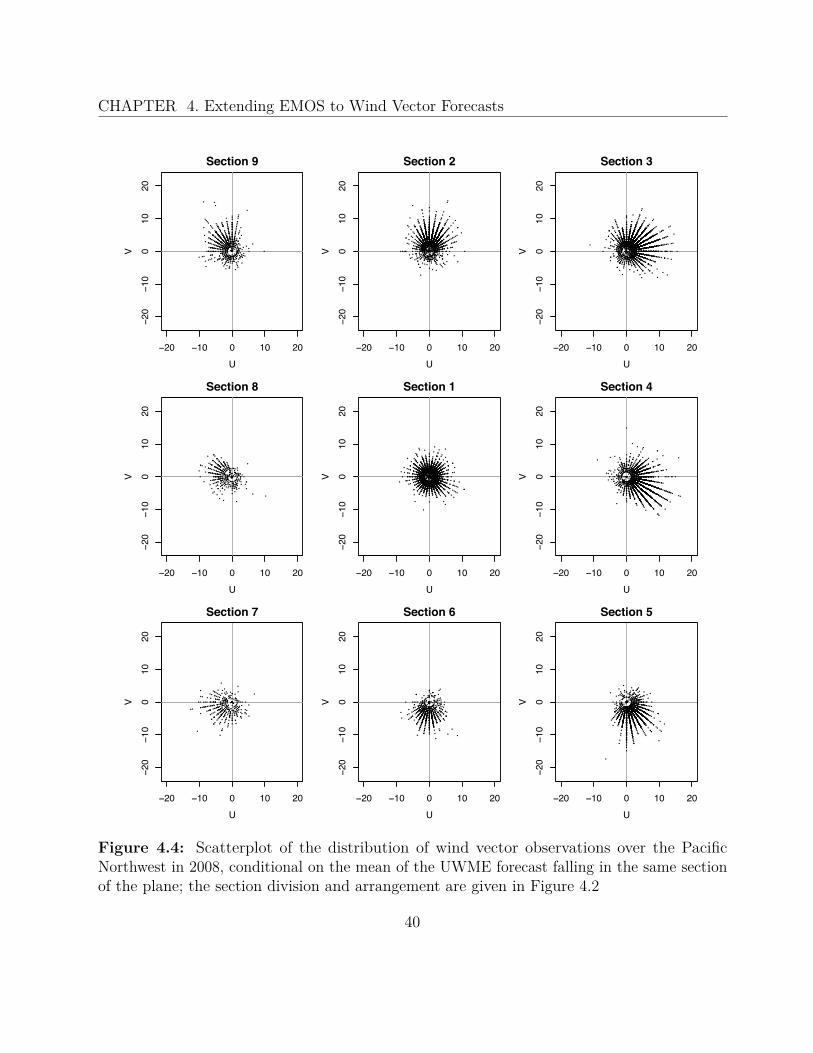
CHAPTER 4. Extending EMOS to Wind Vector Forecasts
−20 −10 0 10 20
−20
−10
010
20
Section 9
U
V
●
●
●
●
●●
●
●
●
●
●
●●●●
●
●
●
●●
●●
●
●
● ●●
●
●●
●
●
●
●
●
●
●
●
●
●
●
●
●
●
●
●
●●
●
●
●
●
●
●
●
●
●
●
●
●
●
●●
●●●
●
●
●
●●
●
●
●
●
●●
●●●
●
●
●●
●
●
●
●
●
●
●
●
●●
●●
●●
●
●
●
●
●
●
●
●
●
●
●
●
●
●
●
●
●
● ●
●
●
●
●
●
●
●
●●
●
●
●
●●
● ●
●
●
●
●
●
●
●
●
●
●
●
●
●
●
●
●
●
●
●
●●
●●●
●
●
●
●
●
●
●
●
●
●
●
●
●
●
●
●
●
●
●
●
●
●
●●
●
●●
●
●
●
●●
●
●
●●
●
●
●
●
●
●
●
●
●
●
●
●
●
●
●
●
●
●●●
●
●
●
●
●●●
●
●
●
●
●
●●
●
●
●
●
●
●
●
●
●
●
●
●
●
●
●
●
●
●●
●
●
●
●●
●
●
●
●
●
●
●
●
●
●
●
●
●
●
●●●
●
●
●
●
●
●●
●
●
●
●
●
●
●
●●●
●
●
●
●
●
●
●
●
●
●
●
●
●
● ●
●
●
●
●●
●
●
●
●
●
●
●
●
●
●
●●
●
●
●
●
●
●
●
●
●
●
●●
●
●
●●
●
●
●
●
●
●
●
●
●
●
●
●●
●
●
●
●
●
●●
●
●
● ●
●
●
●●
●
●
● ●
●
●
●
●
●
●● ●
●
●
●
●
●
●
●
●
●
●
●
●
●
●
●
●
●
●
●
●●
●
●
●
●
●
●
●
●
●
●
●
●
●
●●
●
●
●
●
●●
●
●
●
●
●
●
●
●
●
●●
●
●
●
●
●●
●
●
●
●
●
●
●●
●
●●
●
●●
●
●
●
●
●
●
●
●
●
●
●
●●
●
●
●
●
●
●
●
●
●
●
●
●
●●
●
●
●
●
● ●
●
●
●
●●
●
●
●
●
●
●
●
●
●
●
●
●
●●
●●
●
●
●
●
●
●
●
●●
●
●
●
●
●
●
●
●●
●
●●
●
●
●
●
● ●
●
●
●
●
●
●
●
●
●
●●
●●
●
●
●●
●
●
●
●
●
●
●●
●
●
●●
●
●
●
●
●
●
●●
●●
●
●●
●
●
●
●
●
●
●
●
●
●
●
●
●●● ●●●●
●
●●
●
●
●
●
●
●
●
●
●
●
●
●●
●
●
●
●●
●
●
●●
●
●
●
●
●
●
●●
●
●
●
●
●●
●●
●
●
●
●
●
●
●
●
●
●●●
●
●
●
●
●
●
●
●●
●
●●
●
●●
●
● ●
●
●
●
●
●
●
●
●
●
●
●
●
●
●●
●
●
●
●
●●●
●
●
●
●
●
●
●
●
●
●
●
●
●
●
●
●
●
●
●
●
●
●
●
●
●
●
●●●
●
●●
●
●
●●
●
●
●●
●
●
●
●
●
●
●
●
●
●
●●
●
●
●
●
●
●
●
●
●
●
●
●
●
●●
●
●
●●
●
●
●
●●
● ●●
●
●
●
●
●●
●
●
●
●
●●
●
●●●
●
●
●
●●
●
●
● ●●
●
●
●●
●
●
●
●
●
●
●
●
●
●
●●●
●●
●
●
●
●
●
●
●
●
●
●
●
●
●
●
●
●●
●
●
●
●●
●
●
●
●
●
●
●
●●
●●
●
●●
●
●
●
●
●
●●
●●
●
●
●●●
●
●
●
●
●
●
●●
●
●
●
●
●
●
●
●
●●
●
●
●●●
●
●●
●
●
●
●
●
●
●
●
●
●
●
●
●
●
●
●
●
●
●●
●
●
●
●
●
●
●
●●
●
●
●●
●
●
●
●●
●
●
●
●
●
●
●
●
●
●
●
●
●
●
●
●
●
●
●
●
●
●
●
●
●
●
●
●●
●
●
●
●
●
●
●●
●
●
●
●
●
●●
●
●
●
●●●
●●
●
●
●●
●
●
●
●
●
●
●
●
−20 −10 0 10 20−20
−10
010
20
Section 2
U
V
●
●●●
●
●
●
●
●●
●
●
●
●
●
●
●
●
● ●
●
●
●
●●●
●
● ●
● ●
●
●
●
●●
●●
●
●
●
●
●
●●
●
●
●
●
●
●
●
●
●
●
●●
●
●
●
●
●
●
●
●
●
●
●
●●
●
●
●
●
●
●●
●
●
●
●
●
●
●
●
●●
●
●
●
●●
●●
●
●
● ●
●
●
●
●●
●
●
●
●●
●
●
●
●
●
●
●
●
●
●
●
●
●
●
●
●
●
●
●
●●
●
●●
●
●
●
●
●
●
●
●
●
●
●
●●
●
●
●
●
●
●
●
●
●
●
●●
●
●
●●
●
●●
●●
●
●
●●
●
●
●
●
●
●
●
●
●
●
●●
●
●
●
●
●
●
●
●●
●
●
●●
●
●●
●
●●
●
●
●
●
●
●
●
●
●●●
●
●
●●
●
●
●
●
●
●
●
●
●
●●
●
●
●
●
●●
●
●
●
● ●
●
●
●
●
●
●
●
●
●
●
●
●
●
●
●
● ●
●●
●
●
●●
●
●
●
●●●
●●
●
●
●
●●●
●
●
●
●
●
●●●
● ●
●
●
●
●
●
●
●
●
●
●
●
●●
●
●
●
●
●
●●●
●
●
●●
●
●
●
●
●
●
●
●
●
●●
●
●
●
●
●
●
●
●
●
●
●
●
●
●
●●●●
●
●
●
●
●
●
●
●
●
●
●
●
●
●
●
●
●
●
●●
●
●
●
●
●
●
●
●
●
●
●●●
●
●
●
●
●
●
●
●
●
●
●
●
●
●●
●
●
●
●
●●●
●●
●
●
●
●
●
●
●●
●
●
●
●
●
●
●
●
●
●
●
●
●
●
●
●●
●
●
●
●
● ●
●
●
●
●
●●
●
●
●
●
●
●
●
●
●
●
●
●
●
●
●
●
●
●●
●
●
●
●
●
●
●●
●
●
●
● ●
●
●
●●●
●
●
●
●●
●
●
●
●
●
●
●
●
●
●
●
●
●
●
●
●
●●●
●
●
●●
●●
●
●
●●●
●
●
●
●
●
●
●
●
●
●
●
●
●
●
●
●
●
●
●
●
●
●
●
●
●
●
●
●
●
●
●●
●
●
●
●
●
●●
●●
●
●●
●
●
●
●
●
●
●
●
●
●
●
●
●
●
●●
●
●
●
●
●
● ●
●
●
●
●
●
●
●●
●
●
●
●
●
●
●
●
●
●●
●
●
●●
●
●
●●
●
●●
●
●
●
●
●
●
●
●
●
●●●●
●
●●
●
●
●
●
●
●
●
●●
●●
●
● ●
●
●
●
●●
●
●
●
●●●
●
●
●
●
●
●
●
●
●
●
●●
●●
●
●
●
●
●
●
●
●
●
●
●
●
●
●●
●
●
●
●
●
●●
●●
●
●
●●
●
●●
●
●
●● ●
●
●
●
●
●
●
●
●
●
●●
●
●
●
●
●
●●●
●
●
●●
● ●
●
●
●
●
●●
●
●●
●
●
●
●
●●
●
●
●
●●
●
●
●
●
●
●
●
●●
●●
●
●
●
●
●●
●
●
●
●
●
●
●
●
●
●
●
●
●
●
●
●
●
●
●●
●
●
●●
●
●
●
●●
●
●
●●
●
●
●
●
●
●●
●
●
●
●
●
●
●
●
●
●●
●
●
●
●
●
●
●
● ●
●
●
●
●●
●
●
●
●
●
●●
●
●
●
●
●
●●
●
●
●
●●
●
●
●
●
●
●●●
●
●
●
●
●
●
●
●
●●
●
●
●
●
●
●
●
●
●
●
●
●
●
●
●
●
●
●
●
●
●
●
●
●
●●
●
●
●
●
●
●
●
●
●
●
●
●
●
●
●●●●●
●●●
●
●
●
●
●●
●
●
●
●
●
●
●
●
●
●
●
●●
●
●
●
●
●
●
●●
●
●
●
●
●
●
●
●
●
●
●
●
●
●
●
●
●
●
●
●
●
●
●●
●●
●
●
●
●
●
●●
●●
●
●
●
●
●
●
●
●
●●
●
●
●
●
●
●
●●
●
●●
●
●
●
●●
●
●
● ●●
●
●
●
●
●●
●●
●
●●
●
●
● ●
●
●
●
●
● ●●
●
●
●●
●
●
●
●
●
●
●
●
●●
●
●
●●
●
●
●
●
●●
●●
●●
●
●
●
●
●●
●
●
●
●
●
●
●
●
●
●
●
●●
●
●
●
●
●
●
●
●
●
●
●●
●
●
●
●
●
●
●
●
●
●●
●
●●
●
●
●
●
●
●
●
●●
●
●●
●
●
●
●
●
●●
●
●
●
●
●
●
●
●
●
●
●●
●
●
●
●
●
●
●
●●●
●
●●●●
●
●
●
●
●
●
●
●
●
●
●
●
●
●
●
●
●
●
●
●
●
●
●
●●
●
●
●
●
●
●
●
●●
●
●
●●
●
●
●
●
●
●
●
●
●
●
●
●●
●
●
●
●
●
●
●
●●
●●
●
●
●
●
●
●
●
●
●
●
●
●
●
●
●
●
●
●
●
●
●
●
●●
●
●●
●
●
●
●
●
●
●●
●
●
●●
●
●
●
●
●
●
●
●
●●
●●
●
●
●
●● ●
●●
●
●
●●
●
●●
●
●
●
●
●
●
●
●
●
●
●
●
●
●
●
●
●
●
●
●●●
●
●
●
●●
●
●
●
●
●
●
●●
●●
●
●
●
●
●
● ●
●
●
●
●●
●
●
●
●
●
●
●
●●
●
●
●
●
●
●
●
●
●
●
●
●
●
●
●●
●
●●
●
●
●
●
●
●
●
●
●
●
●
●
●
●
●● ●
●
●
●
●
●
●
●
●●
●●
●
●
●
●●
●
●
●
●
●
●
●
●
●●
●
●
●
●
●
●
●
●●
●
●
●
●
●
●
●
●
●
●
●
●
●
●●
●
●
●
●
●
●
● ●
●
●
●
●
●
●
●
●
●
●
●●
●
●
●
●
●●
● ●
●
●
●
●
●
● ●
●
●
●
●
●
●
●
●●
●
●●
●●
●
●
●
●
●
●
●
●
●●
● ●
●●
●
●
●
●
●
●
●●
●
●
●
●
●
●
●
●
●
●●
●
●
●●
●
●
●
●
●●
●
●
●
●
●
●
●
●
●
●
●
●●
●
●●
●
●
●
●
●
●
●
●
●
●
●
●●
●
●
●
●
●
●
●
●
●
●
●
●
●●
●
●
●
●
●
●
●
●
●
●
●
●
●
●
●●
●
●●
●
●
●
●
●
●
●
●●
●
●
●
●
●
●● ●
●
●
●
●
●●
●
●●
●
●
●●●
●
●
●
●
●
●
●
●
●
●
●
●
●
●
●●
●
●
●
●
●
●
●
●
●
●●
●
●
●
●
●
●●
●
●
●
●
●
●
●
●
●
●
●
●
●
●●●
●
●
●●
●
●
●
●
●●
●
●
●
●●
●●
●
●
●
●
●
●
●
●
●
●
● ●
●
●●
●
●
●
●
● ●
●
●
●
●
●
●
●
●
●
●
●
●
●●
●
●●●
●
●
●●
●
●
●
●
●
●
●
●
●● ●
●
●
●
●
●
●
●
●
●●●
●
●
●
●
●
●
●
●
●
●
●
●
●
●
●
●
●
●
●●
●
●
●
●
●
●
●
●
●
●
●●●
●
●
●
●
●
●
●
●
●
●
●
●
●
●
●
●
●
●
●●
●●
●
●
●
●
●
●●
●
●
●
●
●
●●
●
●
●
●
●
●
●
●
●
●
●
●
●
●
●
●●
● ●●
●
●
●●
●
●
●
●
●
●
●
●
●
●●
●●
●
●
●
●
●
●
●● ●
●
●
●
●
●
●
●
●●
●
●
●
●
●
●
●
●
●
●
●●
●
●●●
● ●●
●
●
●●
●●
●
●●
●
● ●●
●
●●
●
●
●
●
●
●
●
●
●
●
●
●
●
●
●
●●
●
●
●
● ●
●
●
●
●
●
●
●
●
●
●
●
●●
●
●
●
●
●●
●
●
●
●
●
●●
● ●
●
●
●
●●
●
●
●●
●
●●
●
●
●
●
●
●
●
●
●●
●
●
●●
●
●●●
●●
●
●
●●
●
●
●●
●
●
●
●●
●
●
●●
●
●
●
●
●●
●
●
●
●
●
●
●
●
●●
●
●
●
● ●
●
●
●
●
●
●●
●●●●●
●
●
●
●●
●
●
●
●
●
●
●●
●
●
●
●
●
●
●
●
●
●
●
●
●
●
●
●
●
●
●
●
●●
●
●
●
●●
●
●
●●
●●
●
●
●●
●
●
●
●
●
●
●
●
●
●
●●
●● ●
●
●
●
●
●
●
●
●
●
●
●●●
● ●
●
●
●
●
●
●
●
●
●
●●
●
●
●●
●
●
●
●
●
● ●
●
●
●●
●
●●
●
●
●
●
●
●
●
●
●●
●
●
●
●
●
●
●
●
●
●
● ●
●
●
●
●
●
●●
●
●●
●
●
●
●
●●
●
●
●
●
●
●
●
●
●
●
●
●●●
●
●
●
●
●
●
●
●
●
●
●
●
●
●
●
●
●
●
●
●
●
●
●
●●
●
●
●
●
●
●
●
●
●
●
●
●●
●
●●
●
●
●
●●
●
●
●
●●
●●
●
●
●
●
●●
●
●●
●
●
● ●●
●
●
●
●
●
●
●
●
●●
●
●
●
●
●
●
●●●
●
●
●
●●
●
●
●
●●
●
●
●
●
●
●●
●
●
●
●
●
●
●
●
●
●
● ●
●
●
●
●
●
●
●●
●
●
●
●●
●
●
●
●
●
●
●
●
●
● ●●
●
●
●
●
●
●
●●
●
●
●
●● ●●
●
●●
●
●●
●
●●
●
●
●
●
●
●
●● ●
●
●
●
●
●
●
●
●
●
●●
●●
●
●
●
●
●
●●
●
●
●
●●
●
●
●
●
●
●
●
●
●
●
●
●●
●
●
●
●
●
●
●
●
●●
●
●
●
●●
●
●●
●
●
●
●
●
●●
●
●
●
●●
●
●
●
●
●
●
●
●
●
●●●
●
●●
●
●●
●
●
●●
●
●●
●
●
●
●
●
●
●
●
●
●
●
●
●
●
●
●●
●
●
●
●●●●
●
●
●
●●● ●
●
●
●
●
●
●
●
●
●●
●
●
●
●
●
●
●
●
●
●
●
●
●
●
●
●
●
●
●
●
●
●
●
●
●
●
●
●
●
●
●
●
●●●
●
●
●
●●
●
●
●
●
●
●
●
●
●
●
●●
●
●
●
●
●
●
●
●
●
●
●
●
●
●
●
●
●
●
●●
●
●
●
●
●
●
●
●
●
●
●
●
●
●
●
●
●
●
●
●
●
●●
●
●
●
●●
●●
●
●●
●
●●●
●
●
●●
●
●
●
●
●
●
●
●
●
●
●
●
●
●
●
●
●
●
●
●
●
●
−20 −10 0 10 20
−20
−10
010
20
Section 3
U
V
●
●●
●
●
●
●●
●
●
●
●
●
●
●
●
●
●
●
●
●
●
●
●
●
●
●
●●
●
●
●
●
●
●
●
●
●●
●
●
●
●
●
●
●●
●
●
●●
●
●
●
● ●
●
●
●
●
●
●
●
●●
●
●
●
●
●
●
●
●
●●
●
●
●
●
●
●
●
●
●
●
●
●
●
●
●●
●
●●
●
●
●
●
●
●
● ●●●
●●
●
● ●●
●
● ●●●
●
●
●
●●
●●
●●
●●
●
●
●
●
●
●
●
●
●
●
●
●●
●
●●
●
●●●
●
●●
●●
●
●
●
●
●
●
●
●●
●●
●
●●●●
●
●
●●●
●
●
●
●
●
●
●
●
●
●●
●
●
●
●
●
●
●
●
●
●
●
●
●
●
●
●
●
●
●
●
●
●
● ●●
●
●●●
●
●
●
●
●
●●
●
●
●
●●
●
●
●
●
●
●
●●
●
●
●
●
●
●
●
●
●
●
●
●
●●
●
●
●
●
●●
●
●●
●
●●
●
●
●
●
●
●
●
●
●
●
●
●
●
●
●
●
●
●
●
●
●
●
●
●
●
●
●
●
●
●●
●
●●
●
●●
●●
●
●
●
●●
●
●
●●
●
●
●
●
●
●
●
●
●
●
●
● ●
●
●
●
●
●●
●
●
●
●
●
●
●
●
●
●
●●
●
● ●
●
●
●
●
●
●
●
●
●
●
●
●
●
●
●
●
●
●●
●
● ●●
●
●
●
●●
●
●
●
●
●
●●
●
●
●
●
●
●
●
●
●
●
●
●●
●
●
●
●
●
●
●
●
●
●
●
●
●
●
●
●
●
●
●
●
●
●
●
●●
●
●
●
●
●
●
●●
●●
●
●
●
●
●
●
●
●
●
●
●
●
●
●
●
●
●
●
●
●
●
●
●
●
●
●
●●
●
●●
●
●
●●
●
●
●
●●
●
●
●
●
●
●
●
●●
●
●
●
●
●
●
●
●
●
●
● ●
●
●
●
●
●●
●
●
●
●
●
●
●
●
●
●
●
●
●
●
●
●
●
●
●●
●
●
●
● ●
●
●●
●●
●●
●
●
●
●
●
●
●
●
●
●
●
●
● ●
●
●
●
●●
●
●
●
●
●
●
●●
●
●
●
●
●
● ●
●
●
●
●●●
●
● ●●
●
●
●
●
●
●
●
●
●
●●
● ●
●
●
●
●●
●
●
●●
●
●
●
●
●●●●
●
● ●
●
●
●
●
●
●● ●
●
●
●
●●
●
●
●
●
●
●
●
●
●
●
●●
●
●
●
●
●
●
●●
●
●
●
●
●
●
●
●
●
● ●
●
●
●
●
●
●
●
●
●
●
●
●
●
●●
●
●
●
●
● ●
●●
●
●
●●
●
●
●
●
●
●
●
●
●
●
●
●
●
●
●
●
●
●
●
●
●
●
●
●
●
●
●●
●
●
●
●
●
●●●
●
●
●●
●
●
●
●
●●
●
●
●
●
●
●
●
●
●
●
●
●
●
●
●
●●
●
●
●
●
●
●
●
●
●●
●
●
●
●●
●●
●
●
●●●
●
●●
●
●
●
●
●
●
●
●
●
●
●
●●
●
●
●
●
●
●●
●
●
●
●●
●
●●
●
●
●
●
●
●
●
●
●
●
●
● ●
●●
●
●
●
●
●
●
●
●●
●●●
●
●
●
●
●
●
●
●
●●
●●
●
●
●
●
●
●
●
●
●
●
●●
●●
●
●●
●
●
● ●●
●
●
●
●
●
●●
● ●
●●
●
●
●
●
●
●● ●
●●
●
●
●
●
●
●
●
●
●
●●
●
●
●
●
●
●
●
●
●
●
●
●
●
●
●
●
●
●
●
●
●
●
●
●
●
●
●
●
●
●●
●
● ●
●
●
●
●
●●●
●
●
●
●
●●
●
●
●
●
●
●
●
●
●
●
●
●
●
●●●
●
●
●
●●
●
●
●
●
●
●
●
●
●
●
●
●
●
●
●
●
●
●
●
●
●
●
●●
●
●
●
●
●
●
● ●
●
●
●
●
●
●
●●
●●
●●
●
●
●
●
●
●
●
●
●●
● ●
●
●
●
●
●
●
●
●
●
●
●
●
●
●
●
●
●
●
●
●
●
●
●
●
●
●
●
●
●
●
●
●
●
●
●
●
●
●
●
●
●
●
●
●
●
●
●
●
●
●
●
●
●●
●
●
●
●
●
●
●
●
●
●
●●
●
●
●
●
●
●
●●
●
●
●●
●
●
●
●●
●
●
●
●
●●
●
●
● ●●
●
●
●
●●
●
●
●
●
●
●
●●
●
●
●
●
●
●
●
●
●
● ●
●
●●
●
●
●
●
●●
●
●
●
●
●
●
●
●
● ●●
●
●●
●
●
●
●
●
●
●
●●
●
●
●
●
●
●
●●
●●
●
●
●
●
●
●
●
●
●
●
●
●●
●
●
●
●
●
●
●
● ●
●
●●
●
●
●
●
● ●●
●
●
●
●●
●
●
●●
●
● ●
●
●
●
●
●
●
●
●
●
● ●
●
●
●
● ●
●
●
●
●
●
●
●
●
●
●
●
●
●
●
●
●
●
●
●
●
●
●
●
●
●●
●
●
●
●
●
●
●●
●
●
●
●
●
●
●
●
●
●
●
●
●
●
●
●
●
●
●
●
●●
●
●
●●
●
●
●
●
●
●
●
●
●
●
●
●
●
●
●
●
●
●
●
●
●●
●
●●
●
●
●
●
●
●
●
●
●
●
●
●
●
●
●
●
●
●
●
●
●
●
●
●●
●
●
●
●
●
●
●
●
●●
●
●
●
●
●
●
●
●
●●●
●
● ●
●
●
●
●●
●
●
●
●
●●
●
●
●
●
●
●
●
●
●
●
●
●●
●●
●
●
●
●
●
●
●
●
●
●
●●●
●
●
●
●
●
●
●
●
●
●
● ●
●
●●
●
●
●
●
●
●
●
●
●
●
●
●●●
●
●
●
●
●
●
●●
●
●
●
●
●
●
●●●
●●
●
●
●
●
●
●
●●
●
●
●
●
●
●
●
●
●
●
●
●
●
●●
●●
●
●
●
●
●
●
●●●● ●
●
●
●
● ●
●
●
●
●
●
●
●
●
●
●
●
●
●
●●
●
●
●●
●
●
●
●
●
●●
●●
●●
●
●
●
●
●
●
●
●
●
● ●
●
●
●
●
●
●
●
●
●
●
●
●●
●
●
●
●
●● ●
●●
●●
●
● ●
●
●
●
●
●
●
●
●
●●
●
●
●
●
●
●●
●
●
●
●
●
●
●
●
●
●●
●
●
●
●
●
●
●
● ●
●
●
●●
●
●
●
●●
●●
●
●
●
●
●
●●
●
●
●
●
●●
●
●
●
●
●
●
●
●
●
●●
●
● ●
●
●●
●
● ●
●●
●●
●
●
●
●
●●
●●
●
●
●
●
●
●
●
●●
●●
●
●●
●
●
● ●
●
●
●●
●
●
●
●
●
●
●
●
●
●
●
●●
●
●
●
●
●
●● ●
●
● ●
●
●●
●
●
●
●
●●
●●
●
●
●
●
●
●
●●●
●●
●●●
●●
●
●
●
●
●
●
●
●
●
●●
●
●
●
●
●
●●
●
●
●
●
●
●
●
●
●
●
●
●
●
●
●
●
●
●
●
●
●
●
●
●
●
●
●
●
●
●
●
●
●
●
●
●
●
●
●
●
●
●
●
●
●
●
●
●
●
●●
●
●
●
●
●
●
●
●
●
●
●
●
● ●
●
●
●
●
●
●●
●
●
●
●
●
●
●
●
●
●●
●
●
●
●
●
●
●
●
●
●
●
●
●
●
●
●
●●
●
●
●
●
●●
●
●
●
●
●
●
●
●
●
●●
●
●
●●
●
●●
●
●
●
●
●
●●
●
●
●
●
●
●
●
●
●
●
●
●
●
●
●
●
●
●
●
●
●
●
●
●
●●
●
●
●
●
●
●
●
●
●
●
●
●
●●
●●
●
●
●
●
●●
●
●
●
●
●
●
●
●●
● ●
●
●
●
●
●
●●
●
●
●
●
●
●
●
●
●
●
●
●
●
●
●
●
●●
●
●
●
●
●
●●
●
●
●
●●
●
●
●
●●
●
●
●
●●
●
●●
●
●
●
●
●
●
●
●
●
●●
●
●
●
●
●
●
●
●
●●
●
●
●
●
●
●
●●
●●
●
●
●
●
●
●
●
● ●●
●
●
●
●
● ●
●
●●
●
● ●●
●
●●
●
●
●
●●
●
● ●
●●
●●
●
●
●
●
●
●
●
●
●
●
●
●
●
●
●
●
●
●
●
●
●
●
●
●
● ●
●●
●
●
●
●
●
●
●
●
●
●
●
●
●●
● ●
●
●
●
●
●●
●
●●
●
●
●
●
●
●
●
●
●
● ●
●
●
●
●
●
●
●
●
●
●
●
●●
● ●
●
●
●●
●
●
●
●●
●
●●
●
●
●
●
●
●
●
●
●
●
●
●
●
●
●
●
●
●●
●
●
●
●
●●
●
●
●
●
●
●●
●
●
●
●
●
●
●
●
●
●
●
●
●●
●
●●●
●●
●
●
●
●●●
●
● ●
●
●
●
●
●
●
●
●
●
●
●●
●
● ●
●
●
●
●
●
●●
●
●●
●
●
●
●
●
●
●
●●
●
●
●
●
●
●
●●
●
●
●
●
●●
●●
●
●
●
●●
●
●●
●
●
●
●● ●
●
●
●
●
●
●
●
●
●
●
●
●
●
●
●●
●
●
●
●
●
●
●
●
●
●
●
●
●
● ●
●
●
●
●
●
●
●
●●●
●
●●
●
●
●●
●
●●
●
●
●
●
●
●
●
●
●
●
●
●
●
●
●
●
●
●
●
●●
●
●●
●
●
●
●
●
●
●●
●
●
●
● ●
●
●●
●
●
●
●
●●
●
●
●
●
●
●
●
●
●
●
●●● ●
●
●
●●
●
●
●
●
●
●
●
●
●
●●
●●
●
●
●●
●
●
●
●
●
●
●●
●
●
●
●
●
●
●
●
●
●
●
●
●
●
●
●
●
●
●
●
●
●
●●
●
●●●
●
●
●
●
●
●
●
●
●
●● ●●
●
●
●
●●
●
●
●
●
●
●
●
●
●
●●
●●
●
●● ●
●●
●
●●
●
●
●
●
●
●●
●
●
●
●●
●
●
●
●
●
●
●●
●
●
●
●
●
●●
●
●
●
●
●
●
●
●
●
●
●
●
●
●
●
●
●
●
●
●
●
●
●
●● ●
●●
●
●
●
●
●
●
●
●
●
●
●
●●
●
●
●●
●
●● ●
●
●
●
●
●
●
●
●
●
●
●
●
●
●
●
●
●
●
●
●●
●●
●
●
●
●
●●
●●
●
●
●
●
●●●
●
● ●
●
●
●
●●
●
●
●
●
●
●
●
●
●
●
●●
●
●
●
●
●
●
●
●
●●
●
●
●●
●
●
●
●●
●
●
●
●
●
●
●
●
●
●
●●
●
●
●
●
● ●
●
●
●
●
●
●
●
●
●
● ●
●
●
●
●
●
●
●
●
●
●
●●
●
●
●
●
●
●
●
●
●
●
●
●
●●
●
●
●
●
●
●
●●
●
●
●●
● ●
●●
●
●
●
●
●●
●
●
●
●
●
●
●●
●
●
●
●
●●
●
●
●
●
●
●
●
●
●●
●●●
●
●●
●
●
●
●
●
●
●
●
●
●
●
●
●
●●
●
●
●
●
●
●
●
●
●
●
●
●
●
●
●
●
●
●
●
●
●
●
●
●
●●
●
●
●
●●
●●
●
●
●
●
●
●
●
●
●●
●
●●
●
●
●
●●
●
●
●●
●
●
●
●
●●
●
●
●
●
●
●
●
●
●
●
●
●
●
●
●
●
●
●
●
●
●
●
●
●
●
●
●
●
●
●
●
●
●
●
●
●
●
●
●
●
●
●
●●
●
● ●
●
●
●
●
●
●
●
●
●
●
●
●
●
●●●
●
●
●
●●
●
●
●
●●
●
●
●
●
●
●
●
●
●
●
●
●
●
●
●
●
●
●
●
●
●
●
●
●
●
●
●
●
●
●
●
●●
●●
●
●
●
●
●
●
●●
●
●
●
●
●
●
●
●
●
●
●
●
●
●
●
●
●●
●
●
●
●
●
●●
●
●
●
●
●
●
●
●●
●
●
●
●
●
●
●
●
●
●
●
●
●●
●
●
●
●
●
●
● ●
●
●
● ●
●
●
●
●
●
●
●
●
●
●
●
●
●
●
●●
●●
●
●
●●
●
●
●
●
●
●
●
● ●
●
●
●
●
●
●
●
●
●
●
● ●
●●
●
●
●
●
●
●
●
●
●
●
●
●
●
●
●
●
●
●
●
●
●
●
●●● ●
●
●●
●
●
●
●
●
●
●
●
●
●
●
●
●
●
●
●
●
●
●
●
●
●
●
●
●
●
●
●
●
●
●
●●
●
●
●
●
●●●
●
●●
●
●
●
●
●
●
● ●
●
●
●
●
●
●●
●
●●
●
●●
●
●
●●
●
●
●
●
●
●●●
●
●
●●●
●
●
●
●
●
●●
●
●●
●
●
●
●
●
●
●
●
●
●
●
●
●
●
●
●●
●
●
●
●
●
●●
● ●
●
●
●
●
●
●
●
●
●
●
●
●
● ●
●
●●●
●
●●
●
●
●
●●
●
●●
●
●●
●
●
●
●
●
●
●
●
●
●
●
●●
●
●
●
● ●
●
●
●
●
●
●
●
●
●
●
●●●
●
●
●
●
●
●●
●
●●
●●
●
●
●
●
●
●
●
●
●
●●
●
●
●
●
●
●
● ●
●
●
●
●
●
●
●
●●
●●
●
●
●●
●
●
●
●
● ●●
●
●●
● ●
●
●
●
●
●
●
●
●
●●
●
●
●
●
●●
●
●
●●
●
●
●
●
●
●●
●
●
●
●
●
●
●●●●
●
●
●
●
●
●
●
●
●●
●
●
●
●
●
●
●
●●●
●
●
●
●●
●
●● ●
●
●
●
●
●
●●
●
●
●●
●
●
●
●
●
●
●
●
●
●
●
●
●●
●
●
●
●●
●●
●
●
●
●
●
●
●
●
●
●
●
●
●●
●
●●
●
●
●●
●
●
●
●●
●
●
●
● ●●
●
● ●
●
●
●
●
●●
●
●
●
●
●
●
●
●
●
●
●●
●
●
●
●●
●
●
●●
●
●
●
●
●
●
●
●● ●
●
●
●
●
●
●
●●
●
●
●
●●
●●
●
●
●
●
●
●
●●
●
●
●
●
●
●
●
●
●
●
●
●
●●●
●
●
●
●
●
●●
●
●
●
●
●
●
●●
●
●
●
●
● ●●
●
●●
●
●
●
●
●
●
●
●
●
●
●
●●
●
●
●
●
●
● ●
●
●
●
●
●
●
●
●
●
●
●
●
●
●
●
●
●
●
●
●
●
● ●
●
●
●●
●
●
●
●
●
●
●
●
●
●
●
●
●
●
● ●
●
●●
●
●
●
●
●
●
●
●
●●
●●
●
●
●
●
●
●
●●
●
●
●
●
●
●
●
●
●
●●
●
●●
●●
●
●
●
●
●●
●
●
●
●
●
●
●●
●
●●
●
●●
●●
●
●
●
●
●
●
●●●
●
●
●●
●
●
●
●
●
●
●
●
●
●
●
●
●
●
●
●
●●
●
●●●
●
●
●
●
●
●
●
●
●
●
●
●
●
●
●
●
●
●●
●
●
●
●
●
●●
●
●
●
●
●
●
●
●
● ●
●●
●
●
●
●
●
●
●
●
●
●
●●
●
●●
●
●
●
●
●●
●
●
●
●●
●
●
●
●●
●
●
●
●
●●
●
●●
●
●
●
●
●●
●
●
●
●
●●
●
●
●
●
●
●
●
●
●
●
●
●
●
●
●●
●
●
●
●
●
●
● ●
●
● ●
●
●
●
●
●
●
●
●
●●
●
●
●
●
●
●
● ●●
●
●
● ●
●●
●
●
●●
●●
●
●
●
●
●
●
●
●●
●
●
●
●
●
●
●
●●
●
●
●
●
●
●●
●
●
●
●
●●
●
●
●
●
●
●
●
●●
●
●
●
●
●●
●
●
●
●
●
●
●
●●
●
●
●
●
●
●
●
●
−20 −10 0 10 20
−20
−10
010
20
Section 8
U
V
●
●●
●
●
●
●
●●
●
●
●
●●
●
●●
●●
●
●
●
●
●
●
●
●
●●
●
●
●●●
●
●
●●
●
●
●
●
●
●
●
●●
●
●
●
●
●
●
●
●
●
●
●●
●
●
●
●● ●
●
● ●
●
●
●
●
●
●
●
●
●
●
●●
●
●
●
●
●
●
●●
●
●
●●
●
●
●
●
●
●
●●
●
●
●
●
●
●
●●
●●
●
●
●●
●
●
●●
●●
●
●
●
●
●
●
●
●
●
●
●
●
●
●
●
●
●
●
●
●
●
●
●
●
●
●
●
●
●
●
●
● ●●
●
●
●
●
●
●
●
● ●
●
●
●
●
●
●
●
●
●
●
●
●
●
●
●
●●
●
●
●
●
●
●●
●
●
●
●
●
● ●
●
●
●
●
●
●
●●
●
●
●
●
●
●●
●
●●
●
●
●●
●
●●
●
●
●●
●
●
●
●●
●
●
●●
●
●●
●
●
●
●
●●
●
●
●
●●●
●
●
●
●
●●
●
●
●
●
●
●
●
●
●● ●
●
●
●
●
●
●
●
●
●
●
●
●
●
●
●
●
●
●
●
● ●
●
●
●
●
●
●
●
●
●
●
●
●
●
●
●
●
● ●
●
●
● ●
●
●
●●●
●
●
●●
●
●
●●
●●
●
●
●
●
●
●
●
●
●●
●
●
●
●
●
●
●
●
●
●●
●
●
●
●
●●
●
●
●●
●
●
●
●
●
●
●
●
●
●●●
●
●
●
●
●
●
●
●
●
●●●
●
●
●
●
●
●
●
●
●
●
●
●
●
●
●●
●
●●
●
●●
●
●
●
●
●●
●
●
●
●
●
●
●
●
●
●
●
●
●
●
●
●
●
●
●
●
●
●
●
●
●
●●
●●
●
●● ●
●
●
●
●
●●
●
●
●
● ●
●●
●
●
●
●
●
●
●
●
●
●
●
●●
●
●
●●
●
●
●
●
●
●
●
●
●
●
●
●
●
●
●
●
●
●
●
●
●
●
●
●
●
●
●
●
●
●
●
●
● ●
●
●
−20 −10 0 10 20
−20
−10
010
20
Section 1
U
V ●●
●
●
●
●
●●
●●
●
●
●
●●
●
●●●
●
●
●
●●
●
●
●
●
●
●
●●
●
●
●
●
●
●●
●
●
●
●
●
●
●
●●
●
●●
●
●
●
●●
●
●
●
●
●
●
●
●
●●●
●●
●●
●
●
●
●
●●●
●
●●
●
●
●●●
●
●
●●
●●● ●
●●
●●
●
●
●
●
●
●●
●
● ●
●●●
●●
●
●
●●
●
●●
●
●
●
●
●●
●
●●
●
●●
●
●●●●
●
●
●
●
●●
●
●
●
●
●
●●●●●
●
●
●
●
●●
●
●●●●●●●●●●
●●
●●
●
●●
●
●
● ●
●
●●●
●
●●
●
●
●
●
●
●●
●
●
●
●
●●●
●●
●
●
●
●
●●
●
● ●
●
●
● ●
●
●
●
●●●
●
●
●
●●
●●
●
●
●●
●
●
●
●
●
●
●
●
●●
●
●● ●●
●
●
●
●●●●
●
●●
●
●
●
●●
●
●
●
●
●
●
●
●●●
●
●●
●
●
●
●●
●
●
●
●
●●●●
●
●●
●
●
●
●
●
● ●
●
●
●
●
●
●●●
●
●
●
●
●●●●
●
●
●
●
●
●
●
●
●
●
●
●
●
●●
●● ●
●
●
●
●
●●●●●
●
●
●
●
●
●
●
●●
●
●
●
●
●
●
●●
●● ●
●●
●●●●●●●●●●●●
●
●●
●
●
●
●
●
●
●●●●●
●
●
●
●
●
●
●●
●
●●
●
●●●
●●
●
●
●
● ●●
●●
●
●●●
●
●
● ●
●
●
●
●
●
●
●
●
●
●●
●
●●
●
●●
●●
●
●
●
●
●●
●
●
●
●●
●
●
●
●●
●
●
●
●
●
● ●
●
●●
●
●●●
●●●
●
●
●
●
●
●●
●
●
●●
●
●
●
●●
●
●
●
●●
●
●
●
●
●●
●●●
●
●
●
●
●●
●
●
●
●
●
●
●
●
●
●●
●●●
●
●
●●
●
●
●●● ●●●
●●
●●●●●●
●
●
●
●●
●
●●
●
● ●
●
●
●
●
●
●
●
●
●
●
●
●
●●
●●●
●●
●
●
●
●●
●
●
●●●
●
●
●●●●●●
●
●●●
●
●●
●
●●
●
●●
●
●●●●
●●
●●
●
●●●●●
●
●
●
● ●
●●
●
●
●
●
●
●
●●
●
●
●
●
●
●
●
●●
●
●
●
●
●
●●
●
●●
● ●
●
●
●
●
●
● ●
●
●
●
●
●
●
●
●●
●
●
●
●
●●●
●
●
●
●
●
●
●
●
●
●●●
●●
●
●
●
●
●
●
●
●
●●
●
●
●
●
●
●
●
●
●
●
●●
●
●
●
●
●
●
●
●
●
●●
●
●
●
●
●●
●
●
●●
●
●
●
●●
●
●●
●
●●
●●
●
●
●
●
●
●
●
●
●
●● ●
●
●
●
●●
●
●
●
●
●
●●
●
●●
●
●
●
● ●
●
●●
●
●
●
●●
●
●
●
● ●●
●
●●●
●●
●
●
●
●
●
●
●
●
●
●●
●
●
●
●
●
●
●
●
●
●
●
●
●
●
●
●
●
●
●
●
●●●
●
●
●
●
●
●●●
●
●
●
●
●
●
●
●
●
●
●
●
● ●
●
●
●
●
●
●
●
●
●
●
●
●
●
●●
●●
●
●
●
●
●
●
●
●
●
●● ●
●
●
●
●
●●
●
●●
●
●●
●
●
●
●●
●
●
●
●
●
●
●
●
●
●●●
●
●
●
●
● ●
●●●
●
●
●
●
●
●
●●●●
●
●
●
●
●
●●●●●
●
●●●
●
●
●
●
●
● ●
●
●
●
●●●
●
●
●●●●
●
●
●
●
●
●
●
●
●
●
●
●
●
●
●
●
●●
●
●
●●
●
● ●●●
●●
●
●
●
●
●
●
●
●
●
●
●
●
●●
●
●●
●
●●●●●
●
●
●
●
●
●
●●
●
●
●
●
●
●●
●
●
●
●●
●
●
●
●
●
●
●
●
●
●
●
●
●
●
●
●
●●
●
●
●
●
●
●
●
●●●●
● ●●
●
●
●●
●
●
●
●
●●
●
●
●●
●
●
●
●
●●
●
●
●●●
●
●
●
●●
●
●●
●
●
●
●
●
●
●
●
● ●
● ●
●
●
●
●
●
●
●
●
●
●
●
●●
●
●
●
●
●
●
● ●
●
●
●
●●
●
●●
●●
●●
●●●
●
●
●●●
●
●
●●
●●
●●
●
●●
● ●
●
●●
●
●
●
●
●●
● ●
●●
●
●
●
●
●●
●
● ●
●
●
● ●
●
●
●
●●
●
●●●
●
●
●
●
●
●
●
●
●●
●
●●
●
●
●
●
●
●
●
●
●
●
●
●
●●
●
●
●●
●
●●
●
●
●●
●
●
●
●
●●
●
●●●
●
●
●
●
●
●
●
●●
●
●●
●
●
●
●
●
●
●
●
●●
●
●
●●
●
●
●
●
●
●
●
●●
●
●
●●
●
●
● ●
●
●
●
●
●
●●
●
●
●●
●●
●
● ●
●
●
●● ●
●
●
●
●
●
●
●
●
● ●
●●
●
●
●●
●
●
●
●
●
●
●
●
●
●
●
●●●
●
●
●●
●
●
●
●
●
●
●
●●
●●
●
●
●
● ●
●●
●
●
●
●●
●
●
●●●
●
●●
●
●●
●
●
●
●
●
●●●
●
●
●
●
●
●●
●
●
●
●
●
●
●
●
●●
●
●
●
●
●
●
●
●
●●●
●
●
●●
●
●
●
●
●
●●
●
●●
●
●
●
●●
●●
●●
●
●
●
●
●
●
●
●
●
●
●
●●
●
●
●
●
●
●
●
●●
●
●
●●
●
●
●
●
●
●
●
●
●
●
●
●
●
●
●
●
●●
●
●
●
●
●
●
●
●
●●●
●
●
●●●
●
●●
●
●
●
●
● ●
●
●
●●
●
●
●
●
●
●
●
●
●
●
●● ●
●
●
●
●
●●
●
●
●
●
●●
●
●
●
●
●
●
● ●●
●●
●
●
● ●
●
●
●
●
●
●
●
●●
●
●
●
●
●
●●
●●
●
●
●
●
●
●●
●
●
●
●●
●
●
●
●
●●
●
●
●
●
●
●●
●
●●
●
●●
●
●●
●
●
●
●
●
●
●
●
●
●
●
●
●●
● ●
●
●
●
●
●
●
●
●
●●
●●
●
●
●
●
●
●
●
●
●
●
●
●
●
●
●
●
●
●
●
●
●
●●
●
●
●●
●
●
●
●
●
●
●
●
●
●
●
●
●
●
●●
●
●
●
●
●
●
●
●
●
●
●
●
●
●
●
●●
●
●●
●
●
●
●
●
●●
●
●
●
●
●●
●
●
●
●
●
●
●
●
●
●
●
●
●
●●
●● ●●
●
●
●
●
●
●
●
●
●
●
● ●
●
●
●
●
●
●
●
●
●
● ●
●●
●
●●
●●●
●●
●
●
●
●
●
●
●
●
●
●
●
●
●●
●
●
●●
●●
●
●
●
●
●●●
●
●●
●●
● ●
●
●
●
●
●
●
●
●
●●
●
●●
●
●
●
●
●
●●
●
●
●●
●
●
●
●● ●
●
●
●
●
●
● ●
●
●●
●● ●●
●●
●
●
●
●
●
●
●
●
●
●●
●
●
●
●
●●
●
●
●
●
●
●
●
●
●●
●
●
●
●
●
●
●●
●
●
●●
●
●
●
●
●
●
●
●
●
●●●
●●
●
●
●
●
●
●
●
●
●●●
●
●
●●
●
●●
●
●●
● ●
●
●
●
●
●●
●
●
●
●
●
●
●
●
●●
●
●
●
●
●● ●
●●●
●
● ●
●
●
●
●
●
●
●
●●
●●
●
●
●
●
●
●
●
●
●
●
●
●
●
●
●
●●●
●
●
●
●
●
●
●
●
●
●
●
●
●
●
●
●●
●●
●●
●
●
●
●●
●
●
●
●
●
●
●
●
●
●
●
●
●●
●
●
●
●●●
●
●
●●
●
●
●
●
●
●
●
●
●
●
●
●
●
●
● ●●
●
●● ●
●
●
●
●●
●
●●
●
●
●
●
●
● ●●●
●●
●
●
●
●●●
●●
●
●
●
●
●
●
●
●
●●
●
●● ●
●
●●
●
●
●● ●
●
●
●
●
●
●
●
●
●
●
●
●
●●
●
●
●●
●
●
●
●
●
●●
●
●
●
●
●
●
●
●
●
●
●
●
●
●
●
●
●
●
●●
●
●
●
●
●
●
●
●
●
●
●●
●
●
●
●
●
●
●
●
●
●
●
●
●
●
●
●
●
●
●
●
●
●
●
●
● ●
●
●
●
●
●
●
●
●
●
●
●
●
●
●
●
●
●●
●
●
●●
●●
●
●
●
●
●
●
●
●
●
●●
●
●●
●
●
●
●
●
●
●
●
●
●
●
●
●
●
●
●
●
● ●
●
●
●
●
●
●●●
●
●
●●
●
●
●
●
●
●
●
●
●
●●
●
●
●●
●
●
●
●
●
●
●
●
●
●
●
●
●●
●
●
●
●
●
●
●●
●●
●
●
●
●
●●
●
●
●
●
●
●
● ●
●
●
●
●
●
●●
●
●
●
●
●
● ●
●
●●
●
●
●●●
●
●
●
●
●
●
●
●
●
●●
●
●
●●
●
●
●
●
●
●
●
●
●
●
●
●
●
●
●
●
●
●
●
● ●
●
●
●
●
●
●
●
●
●
●
●
●
●
●
●
●
●
●
●●
●
●
●
●
●
●
●
●
●
●
●
●
●
●
●●
●
●
●
●
●
●
●
●●
●
●
●
●
●
●
●●
●
●
●●
●
●
● ●
●
●
●
●
●
●
●
●
●
●
● ●
●●
●
●
●
●
●
●
●
●
●
●
●●
●
●
●
●
●
●
●
●
●
●
●
●
●
●●
●
●
●
●
●
●
●
●
●
●
●
●
●
●
●
●
●
●
●
●
●
●
●●
●
●
●
●●
●
●
●
●●
●●
●
●●
●
●
●
●
●
●●
●
●
●●
●
●
●
●
●
●
●●
●
●
●
●
●
●●
●
●
●
●
●
●
●
●
●
●
● ●
●
●
●
●●
●
●
●●
●●
●●
●
●
●
●
●●
●
●
●
●
●●
●
●●●
●
●
●
●
●
●
●
●
●●●
●
●
●●
●
●
●
●●
●
●●
●
●
●
●●
●
●
●
●●
●
●
●
●
●
●
●●●
●
●●
●
●
●
●
●● ●
●
●●
●
●
● ●
●
●
●
●
●
●
●
●●●
●
●
●
●
●
●
●
●
●
●
●
●
●
●
●
●
●
●
●
●
●
●
●
●
●
●
●
●
●
●
●
●
●
●
●
●
●
●
●
●
●●
●
●
●
●
●
●●
●
●
●●
●
●
●●
●
●
●
●
●
●●
●
●●
● ●
●
●
●●
●
●
●●
●●
●●●●
●
●
●
●
●
●
●
●
●
●
●
●
●
●
●
●
●
●
●
●
●
●●
●
●
●
●
●
●●
●
●
●
●
●●
●
●
●
●
●
● ●
●
●
●
●
●
●
●
●
●
●
●●
●
●●
●
●
●
●
●
●
●
●
●
●●
●
●
●
●
●
●
●●
●
●
●
●
●
●
●
●
●
●●●
●●
●
●
●
●
●
●●
●
●
●
●●
●
●●
●
●
●
● ●
●
●●
●
●
●
●
●
●
●
●
●
●
●
●
●
●
●
●
●●
●
●
●
●
●
●
●
●
●
●
●
●
●
●
●●
●
●●●
●
●
●
●
●
●
●
●
●
●
●
●
●●
●●
●
●
●
●
●
●
● ●●●
●
●
●
●
●
●●
●
●
●
●
●
● ●
●●
●
●
●
●●● ●
●
●
●
●●●●
●
●●
●
● ●
●●
●
●
●
●
●
●
●
●
●
●
●
●
●
●
● ●
● ●
●●
●
●●
●
●
●
●
●
●●
●
●
●●
●
●
●
●
●
●
●
●
●●●
●
●
●
●
●
●
●
●
●
●
●
●
●
●
●●
●●
●●
●
●● ●
●
●
●
●
●
●
●●
●●
●
●●
●
●
●
●
●●
●
●
●●●●●
●
●
●
●●
●
●
●
●
●
●
●
●●
●
●
●
●●
●
●
●
●●
●
●●
●
● ●●
●
●
●
●
●
●
●
●
●
●●●
●
●●
●
●
●
●
●
●
●
●
●
●●
●
●
●
●
●●
●
●●
●●
●
●
●
●
●●
●
●
●
●
●
●●
●●●
●●
●
●●
●
●
●
●
●
●
●
●
●
●
●
●
●
●●
●●
●
●
●
●
●
●●
●
●●●●
●
●●
●●
●
●●
●●
●
●
●
●●
●
●
●
●
●●
●
●
●
● ●●●
●
●●●
●
● ●●
●
●
●
●
●
●●
●
●●●
●
●
●
●
●
●●
●
●
●
●
●●
●●
●
●
●●
●
●
●
●
●
●
●
●
●
●
●
●●
●
●
●
●
●
●
●
●
●
●
●
●
●●
●
●
●●
●
●
●
●
●
●
●
●
●
●
●
●
●
●
●
●
●
●
●
●●
●
●
●
●●
●
●
●
●●
●
●
●
●
●
●
●
●
●
●
●
●
●●
●
●
● ●
●
●
●
●
●
●
●
●●
●●●●
●●●●
●
●
●
●
●
●
●
●
●
●●●
●
●
●
●
●
●
●●●
●
●
●●●
●
●
●
●
●●
●
●
●
● ●
●
●
●
●
●
●
● ●
●
●
●
●●
●
●
●
●
●
●
●●●●
●
●●
●
●
●
●
●
●
●
●
●
●
●●
●
●
●
●
●
●
●
●
●
●
●
●
●
●
●
●
●
● ●
●
●
●
●
●
●●
●
●
●
●
●
●
●
●
●
●
●
●
●
●
●●●●
●
●
●
●
●●
●
●
●
●
●
●●
●
●
●
●
●
●
●
●●
●
●
●
●
●
●●
●
●●●●●
●
●
●●
●
●
●
●
●
●
●
●
●
●
●●
●●
●●
●
●
●
●
●
●
●
●
●
●
●
●
●
●
● ●
●
●
●
●●●
●
●
●
●
●
●
●
●
●
●
●●
●
●
●
●
●
●
●
●
●●
●
●
●
●
●
●
●
●
●
●
●
●
●
●
●
●
●
●
●
●
● ●
●
●
●
●
●
●
●
●
●
●●●
●
●●
●
●
●
●
●●
●
●●
●
●
●
●
●
●
●
●●
●
●
●●
●
●
●
●
●
●
●
●
●
●
●
●
●
●
●
●
●●
●
●
●
●
●
●
●●
●
●●
●
●
●
●
●
●
●
●
●
● ●
●●
●●
●
●
●●
●●●
●
●
●
●
●
●●
●
●●
●
●
●
●
●
●
●
●
●
●
●
●
●
●
●
●
●
●
●●
●
●
●
●●●●●
●
●●
●
●●●●●●●● ●
●
●
●
●
●
●●
●
●
●
●
●
●●
●●
●●
●
●
●
●●
●●
●
●
●
●
●
●●
●
●
●●
●
●
●●
●
●
● ●
●
●
●
●
●
● ●
●●
●
●●
●
●
●
●
●
●
●
● ●●
●
●
●
●
●
●●
●
●●
●
●
●
●
●
●
●
●
●
●●
●
●
●
●
●
●
●
●
●
●
●
●
●
●
●
●●
●●
●
●●
●
●
●
●
●● ●
●
●
●●
●●
●
●●
●●
●
●●
●
●●●
●
●
●
●
●●●●●
●
●●
●
●
●
●
●
●
●●●●
●
●
●
●●●
●
●
●
●
●
●
●
●
●
●●
●
●●
●
●
●●
●
●
●
● ●●
●
●
●●
●
●
●
●
●
●
●
●
●
●
●
●
●
●
●
●
●
●
●
●
●
●
●
●
●
●
●
●●
●
●●● ●
●
●
●●
● ●●
●
●
●
●
●
●
●
●
●
●
●
●
●●●
●●●●
●●
●
●
●
●●
●
●
●
●
●
●
●●
●
●●●●● ●
●
●●●●
●
●●●●
●
●
●●
●●
●
●
●
● ●
●
●●
●●●
●
●
●
●
●
●
●
●
●
●
●● ●●●
●
●●
●
●●
●
●●●
●
●
●●●●●●
●
● ●●●●
●
●●
●
●
●●●
●
●
●
●
●
●
●
●
●
●
● ●
●
●
●●
●
●
●
●
●
●
●
●
●
●
●
●● ●
●
●
●
●
●
●
●●●
●●
●●
●
●●●●●
● ●
●
●●
●●●● ●●
●
●●●
●
●
●●
●
●
●
●
●
●●
●
●
●
●
●
●
●
●
●
●
●
●
●
●
●
●
●
●
●
●
●
●
●
●●●
●
●
●
●●●
●●
●
●●
●
●
●
●
●
●
●
●●
●
●
●
●
●
●
●
●
●
●●●
●
●
● ●●●
●
●
●●●●
●
●
●
●
●
●
●
●
●
●●
●
●
●
●
●●
●
●●
●
●
●●
●●
●●●●
●
●●
●
●
●●
●
●
●
●
●
●
●●●
●
●●
●
●●
●
●
●
●
●
●
●
●●
●
●
●●
●
●●
●
●●
●
●
●
●
●●
●
●●●●
●
●●●●
●●
●●●●
●
●●●●
●
●●
●
●
●●
●
●●
●●
●
●●
●
●●●
●
●●
●
●
●
●
●
●●●●●
●
●● ●
●
●● ●●
●
●
●
●●●
●
●
●
●●●
●
● ●
●
●
●
●
●
●
●
●
●
●
●●●
●
● ●●
●
●●●●
●
●
●
●●
●
●
●
●●
●
●●
●
●
●
●
●
●
●
●●
●
●
●
●●
●
●
●
●
●●
●
●
●
●
●●
●
●
●
●
●●
●●●●
●
●
●
●
●
●
●
●
●
●
●
●
●
●●●
●
●
●●
●
●●
●
●
●
●
●
●
●●
●
●
●
●
●
●
●●
●
●
●●●
●
●●
●
●●
● ●
●
●
●●
●●●●
●
●
●
●
●
●
●
●
●
●●
●●
●
●
●
●
●● ●●
●
●
●
●
●
●●
●
●
●
●
●
●
●●●●
●
●
●
●●
●
●
●●
●
●●●●
●
●
●
●
●●
●●
●
●
●
●
●
●●
●
●●●
●●●
●
●
●●
●
●●
●●
●
●
●
●
●
●
●
●●
●
●●
●
●●
●●
●
●
●
●●
●
●
●
●
●●●
●
●
●
● ●
●
●
●
●
●
●
●
●●
●
●
●
●●
●
●●
●●
●
●
●
●●
●
●
●●●●
●
●
●
●●
●
●●
●
●
●
●
●●
●
●
●
●
●
●
●
●●
●
●
●
●
●
●●●
●●
●
●●
●
●
●●
●
●
●
●●
●
●●
●
●
●
●
●
●●●●●●
●
●
●●
●
●
●●●●●●
●
●
●
●
●
●
●● ●
●●
●
●●
●●
●●
●
●
●●
●
●●
●
●●●
●
●
●
●
●
●
●●●● ●
●
●
●
●●●●●●
●
●●●
●
●
●
●●
●
●
●
●
●
●●
●
●
●●
●
●
●●●
●
●●●
●●
●●●●
●
●
●
●
●
●
●
●●
●
●●●●
●
●●●●
● ●
●
●
●
●● ●
●
●
●
●
●
●
●
●●
●
●●
●
●
●
●●
●
●
●
●
●
●
●
●
●
●
●●●
●
●
●
●
●
●
●●●
●
●●
●
●●
●
●
●
●
●
●
●●
●
●
●●●●
●
●
●
●
●
●
●●
●
●●●
● ●
●
●
●
●
●
●
●
●
●
●
●
●
●●
●●
●
●
●
●
●
●
●
●
●
●
●
●
●
●
●
●
●
●●
●
●
●
●
●
●
●
●
●
●
●
●
●●●
●●
●
●
●
●
●
●
●
●
●
●
●
●●
●
●
●●
●
●●●●●●
●
●
● ●●
●
●
●
●●●
●
●
●
●● ●
●
●
●
●
●●
●
●
●
●
●
●●
●
●
●
●
●●
●
●
●
●
●
●
●
●
●● ●
●
●
●
●●● ●●
●
●●
●
●
●
●
●
●
●
●
●
●
●
●●
●
●
●
●●
●●
●
●
●
●
●
●
●
●●●
●
●
●
●
●
●
●
●
●
●
●
●
●
●
●
●
●
●●●
●
●
●●
−20 −10 0 10 20
−20
−10
010
20
Section 4
U
V ●
●
●
●
●
●●
●
●
●
●●
●
●
●●
●
●
●
●
●
●
●●
●
●●
●
●
●
●●●●
●
●
●
●
●
●
●
●
●
●
●
●
●●
●●●
●
●
●
●
●
●
●
●
●
●
●
●
●
●
●
●
●●
●
●
●
●
●
●
●
●
●
●
●●
●
●
●
●●
●
●
●●
●●
●
●
●
●
●
●
●
●
●
●
●
●
●
●
●
●
●
●
●●
●●
●
●
●
●●
●●●
●
●
●
●
●
●
●
●●●
●
●
●
● ●
●
●
●
●
●
●
●
●
●
●
●
●
●
●
●
●●
●
●
●
●
●●
●
●
●
●
●
●
●●
●
●
●
●
●
●
●
●
●
●
●
●
●
●
●
●
● ●
●
●
●
●
●
●
●
●
●●
●
●
●
●
●
●
●
●
●
●
●
●
●
●
●●
●
●●
●
●
●
●
●
●
●
●
●
●
●
●
●
●●
●
●
●
●
●
●
●
● ●
●
●●
●
●
●
●
●
●
●
● ●
●
●
●
● ●
●
●
●
●●
●
●●
●
●●
●
●
●
●
●
●●
●
●
●
●
●
●
●
●
●
●
●
●
●
●
●
●●
●
●
●
●
●●
●
●
●
●
●
●
●
●
●
●
●
●
●
●
●●
●
●
●
●
●
●
●
●
●
●
●
●
●
●
●
●
●
●
●
●
●
●
●
●
●
●
●
●
●
●
●
●
●
●
●
●●●
●
●
●●
●
●
●
●
●
●
●
●
●
●
●
●
●
●
●
●
●
●
●●●
●
●
●
●
●●
●
●
●
●
●
●
●
●
●
●
●●
●
●
●
●
●
●
●
●
●
●
●
●
●
●
●
●
●
●
●
●
●
●
●
●
●
●●
●
●
●●
●
●
●
●
●
●●●
●
●
●
●
●
●
●
●
●
●
●
●
●
●
●
●
●● ●
●
●
●
●
●
●
●
●
●
●
●
●
●
●●
●●
●
●
●
●
●●
●
●
●
●
●
●
●
●
●
●
●
●
●
●
●
●
●
●
●
●
●
●●
●
●
●
●
●
●
●
●
●
●
●
●●
●
●
●
●
●
●
●
●
●
●
●
●
●
●
●
●
●●
●
●
●
●
●●
●
●
●●
●
●
●
●
●●
●
●●
●
●
●
●
●●
●
●
●●
●
●●
●
●
●
●
●
●
●
●
●
●
●
●
●
●
●
●
●
●
●
●
●
●
●
●
●
●
●
●
●
●
●
●
●
●●
●●
●
●
●●●
●
●●
●
●●
●
●
●
●
●●
●
●
●
●
●
●●
●
●
●
●
●
●
●
●
●
●
●
●
●●
●
●
●
●
●
●
●
●
●
●
●
●●
●
●
●
●●
●
●
●
●
●
●
●
●
●
●
●
●
●
●
●
●
●
●
●
●
●
●
●
●
●
●
●●
●
●
●
●
●
●
●
●
●
●●
●
●
●
●
●
●
●
●
●
●
●
●
●
●
●
●
●
●
●
●●
●
●
●●
●
●
●
●
●●
●
●
●
● ●●
●
●
●
●
●●
●
●
●
●
●
●
●
●
●
●
●
●
●
●●
●
●
●
●
●
●
●
●
●
●
●
●
●
●●
●
●
●
●
●
●
●
●
●
●
●
●
●
●
●●
●
●
●
●
●●
●
●
●
●
●
●
●
●
●
●
●
●
●
●
●
●
●
●
●
●
●
●
●
●
●●
●
●
●
●
● ●
●
●
●
●
●
●
●
●●
●
●
●
●
●
●
●
●
●
●
●
●
●
●
●●
●
●
●
●
●
●
●
●
●
●
●
●
●
●
●
●
●
● ● ●
●
●
●
●
●
● ●
●
●
●
●
●
●
●
●
●
●
●
●●
●
●●
●
●
●
●
●
●
●
●
●
●
●
●
●
●
●
●
●
●
●
●
●
●
●
●
●
●
●
●●
●
● ●
●
●
●
●
●
●
●
●
●
●
●
●
●●
●
●
●
●
●
●
●
●
●
●
●●
●●
●
●
●
● ●
●●
●
●
●
●
●
●
●
●
●
●
●
●
●●
●
●
●
●
● ●
●
●
●
●
●●
●
●
●
● ●
●
●
●●
●
●●
●●
●
●
●●
●
●
●
●
●
●
●
●●
●
●
●
●
●
●
●
●
●
●
●
●●
●
●
●
●●
●
●
●
●
●
●
●
●
●
●
●
●
●
●
●
●
●
●●●
●●
●
●
●
●
●
●●
●
● ●●
●
●
●
●
●
●
●
●
●
●
●
●
●
●
●
●
●
●
●
●
●
●
●
●
●
●●
●
●
●
●
●
●
●
●
●
●
●
●
●
●●
●
●
●
●
●
●●
●
●
●
●●
●
●
●
●
●
●
●
●
●
●
●
●
●
●●
●
●
●
●
●
●
●
●
●
●
●
●
●
●
●
●
●
●
●
●
●
●
●
●●
●●
●
●
●
●
●
●
●
●
●
●
●
●
●
●
●
●
●
●
●
●●
●
●
●
●
●
●
●
●
●
●
●
●
●
●
●
●
●
●
●
●
●
●
●
●
●
●
●
●
●
●
●
●
●
●
●
●●
●
●
●●
●
●●
●
●
●
●
●●
●
●
●
●
●
●
●
●
●
●
●●
●
●
●
●
●
●●
●
●●
●
●
●
●
●
●
●●
●
●●
●
●
●
●
●
●
●
●
●
●
●
●
●● ●
●
●
●
●
●
●●
●
●
●●
●●
●
●
●
●
●
●●
●
●
●
●
●
●
●
●
●
●
●
● ●
●
●
●
●
●
●
●
●
●
●
●
●●
●
●
●
●
●
●
●
●
●
●●
●
●
●
●●
●
●
●
●
●●
●
●
●
●
●
●
●
●
●
●
●
●
●
●
●
●
●
●
●
●
●
●
●
●
●
●
●
●●
●
●
●
●●
●
●
●
●
●
●
●
●●
●
●
●
●
●
●
●
●●
●
●
●
●
●
●
●
●
●●
●
●
●
●
●
● ●
●
●
●
●
●
●
● ● ●
●
●
●
●
●
●
●
●
●
●●
●
●●
●
●
●
●
●
●●
●
●
●
●
●
●
● ●●
●
●
●
●
●
●●
●
●
●
●
●
●
●
●
●●
●
●
●
●
●
●
●
●
●
●
●
●
●
●
●●
●
●●
●
●
●
● ●
●
●
●
●
●
●
●
●●
●
●
●
●
●
●
●
●
●
● ●
●
●●
●
●
●
●
●
●
●
●
●
●
●
●
●
●
●
●
●
●
●
●
●
●
●
●●
●●●
●
●
●
●
●
●●
●
●
●
●
●
●
●●
●●
●
●
●●
●
●
●
●
●●
●
●
●
●
●
●
●
●
●
●
●
●
●
●
●
●●
●
●
●
●
●
●
●
●
●
●
●
●
●
●
●
●
●
●
●
●
●
●
●
●
●
●
●
●
●
●
●
●
●
●●
●
●
●
●
●
●
●
●
●
●
●
●
●
●
●
●
●
●
●
●
●
●
●
●
●
●
●
●
●
●
●● ●
●
●
●
●
●
● ●
●
●
●
●
●
●
●
●
●
●
●
●
●
●
●
●
●
●
●
●●
●
●
●
●
● ●
●
● ●
●
●
●
●
●
●
●
●
●
●
●●
●●
●
●
●
●
●
●●
●
●●
●
●
●
●●
●●
●
●
●
●
●
●
●●
●
●
●
●
●
●
●
●
●
●
●
●
●
●
●
●
●●
●
●
●
●
●
●
●
●
●
●
●
●
●
●
●●
●●
●
●
●
●
●
●
●
●
●
●
●●
●●
●
●
●
●
●
●
●●
●
●
●
●
●
●
●
●
●
● ●
●
●
●
●
●
●
●
●
●
●
●
●
●
●
●
●
●
●
●
●
●
●●
●
●
● ●●
●●
●
●
●
●
●
●
●
●
●●
●
●
●
●
●
●
●
●
●
●
●
●
●
●
●●
●
●
●
●
●
●
●
●
●
●
●
●
●
●
●
●●
●
●
●
●
●
● ●
●
●
●
●
●
●
●
●
●
●
●
●
●●
●
●
●
●
● ●●
●
●
●
●●
●
●
●
●
●
●
●
●
●
●
●
●
● ●
●
●
●
● ●
●●
●
●
●
●
●
●
●
●
●
●
●
●
●●
●●
●
●
●
●
●
●
●
●
●
●
●
●
●
●
●
●
●
●
●
●
●
●
● ●
●
●
●
●
●
●●
●
●●
●●
●
●
●
●
●
●
●
●
●
●
●
●
●
●
●
●
●
●
● ●
●
●●
●
●
●
●
●
●
●
●
●
●
●
●
●●
●
●
●●
●
●●
●
●
●
●●
●
●
●●
●
●
●
●●
●
●
●
●
●
●
●●
●
●
●
●
●
●
●
●
●
●
●
●●
●●
●
●
●
●
●
●
●
●
●
●
●
●
●
●
●
●
●
●
●
●
●
●
●
●
●
●
●●
●
●
●
●
●
●
●
●
●
●
●
●
●
●
●
●
●
●
●●
●
●
●
●
●
●
●
●
●
●
●
●
●●
●
●●
●
●
● ●
●
●
●
●
●
●●
●
●
●
●
●
●
●
●●
●
●
●
●
●
●
●
●●
● ●
●
●
●
●
●
●
●
●
●
●
●
●
●
●●
●
●
●
●
●
●
●
● ●
●
●
●
●
●
●
●
●
●
●●
●
●
●
●
●
●
●
●
●
●
●
●
●
●
●●
●
●
●
●
●●
●● ●
●
●
●
●
●
●
●
●
●
●
●
●
●
●
●
●
●●
●
●●
●
●
●
●
●
●
●
●
●
●
●●
●
●
●
●
●
●
●
●
●
●
●
●
●
●
●
●
●
●
●
●
●
●
●
●
●
●
●
●
●
●●●
●
●
●●
●
●●
●
●
●
●
●
●
●
●
●
●
●
●●
● ●
●
●
●
●
●●
●
●
●●
●
●
●
●
●
●
●
●
● ●
●
●
●●
●
●
●
●
●●
●
●
●
●
●
● ●●
●
●
●
●
● ●
●●●
●
●
●
●
●●
●
●●
●
●
●
●
●
●
●
●
●
●
●
●
●
●
● ●
●
●
●
●
●
●
●
●
●
●
●
●
●
●
●
●
●
●
●
●
●
●
●
●
●
●●
●
●
●
●
●
●
●
●
●
●
●
●
●●
●
●
●
●●
●
●
●
●
●
●
●
●
●●
●
●
●●
●●
●
●
●
●
●
●
●●
●
●●
●
●
●●
●
●
●
●
●
●
●
●
●
●
●
●
●●
●
●
●
●
●
●
●
●
●●
●●
●
●
●
●
●
●
●
● ●
●
●●
●
●
●
●
●
●
●
●
●●
●
●
●
●
●
●●
●
●
●
●
●
●
●
●
●
●
●●
●
●●
●
●●
●
●
●
●
●
●
●
●
●
●
●
●
●
●
●● ●
●
●
●●
●
●
● ●
●
●● ●
●
●
●●
●
●
●
●
●
●
●
●
●
●●
●
●●
●
●
●
●
●
●
●
●
●
●
●
●
●
●
●
●
●
●
●
●
●
●
●
●
●
●
●
●
●
●
●
●
●
●
●
●
●
●
●
●
●
●
●●
●
●
●
●
●
●
●
●
●
●
●
●
●
●
●
●
●
●
●
●
●●
●●
●
●
●
●
●●
●
●
●
●
●
●
●
●
●
●
● ●
●
●
●
●
●
●
●
●
●●
●
●
●
●
●
●
●
●
●
●
●
●
● ●
●
●
●
●
●
●
●
●
●
●
●
●
●
●
●
●●
●
● ●
●
●
●●
●
●
●
●
●
●
●
●
●
●●
●
●
●
●
●
●●
●
●
●
●
●
●
●●
●
●
●
●●
●
●
●
●
●
●
●
●
●
● ●
●
●
●
●
●
●●
●
●
●
●
●
●
●
●
●
●
−20 −10 0 10 20
−20
−10
010
20
Section 7
U
V ●
●
●
● ●
●
●●
●
●
●
●
●
●
●
●●
●
●
●
●
●
●
●
● ●●
●
●
●●
●●
●●
●
●
●
●
●
●
●
●
●
●
●
●
●●
●
●
●
●
●
●
●
●
●
●
●
●
●
●
● ●●
●
●
●
●
●●
●
●
●●
●
●
●
●
●
●
●
●
●●
●
●
●
●
●●
●
●
●
●
●
●
●
●
●
●●
●
●●
●
●
●
●
●
●
●
●
●
●
●●
●
●
●
●
●
●
●
●
●
●●
●
●●
●●
●●
●
●
●
●
●
●
●
●
●
●
●
●
●
●
●● ●
●
●●
●
●
●
●
●
●
●
●
●
● ●
●●
●
●
●
●
●
●
●
●
●
●
●
●
●
●
●
●
●
● ●
●●
●●
●
●
●
●
● ●
●
●
●
●●●
●
●
● ●●●
●
●
●
●
●
●
●
●
●
●
●
●
●
●
●
●
●● ●
●
●
●
●
●
●
●
●
●
●
●
●
●
●
●
●
●
●
●
●
●
●
●
●●
●
●
●
●
●
●
●●
●
●
●
●
●
●
●
●
●
●●
●
●
●
● ●
●● ●
●
●●
●
●
● ●
●
●
●
●●
●
●
●
●
●
●
●
●
●
●
●
●●●●
●
●
●
●
●●
●●
●
●
●●
●
●
●
●
●
●
●
●
●
● ●
●
●
●
●
●
●
●
●
●
●
●
●
●
●
●
●
●
●
●
●
●
●
●
●
●●
●
●
●●
●
●
●
●
●
●
●
●●
●
●●
●
●
●
●●
● ●●
●●
●● ●
●●
●
●
●
●
●
●
●
●
●
●
●
●
●
●
●
●
●
●
●
●
●
●
●●
●
●
●
●●
●
−20 −10 0 10 20
−20
−10
010
20
Section 6
U
V
●
●
●
●
●
●
●●
●
●
●●
●●
●●
●
●●
●
●
●
●
●
● ●
●●
●
●
●
●
●
●
●
●
●
●
●
● ●
●
●
●
●
●
●
●
●●
●
●
●
●
●
●
●
●
●
●
●
●
●
●
●●
●
●●
●
●
●
●
●●
●
●
●
●
●
●
●
●
●
●
●
●
●
●
●
●
●●
●
●●
●
●●
● ●
●
●
●●●
●
●
●
●
●
●●
●
●
●
●●
●
●
●
● ●
● ●●
●●
●
●
● ●●
●
●●
●
●
●
●
●
●
●●
●
●
●●
●
●
●
●
●
●
●●
●
●
●●
●
●● ●
●●
●
●
●
●
●●
●
●●
●
●
●●
●
●
●
●
●
●
●●
●
●
●
●
●
●
●
●
●
●
●
●
●●
●
●
●
●●
●
●●
●
●●
●
●
●
●●
●
●●
●
●
●
●●● ●
●
●
●
●
●
●
●
●●
● ●●●
●
●●
●
●
●
●
●
●
●
●
●
●
●
●
●
●
●●●
●●
●
●
●
●
●
●
●
●
●
●
●●
●
●
●
●
●
●
●
●
●●
●
●
●
●
●
●
●
●
●
●●
●
●
●
●
●
●●
●●
●
●
●●
●
●
●●
●
●
●
●●
●●
●
●
●
●
●
●
●
●●
●
●●
●
●
●
●
●
●
●
●
●
●●
●
●
●
●
●●
●
●
●
●
●
●
●
●
●
●
●
●
●
●
●
●
●
●
●
●
●
●
●
●●
●
●
●
●
●
●
●
●
●
●
●
●
● ●
●
●●
●
●
●
●
●
●
●
●
●
●
●
●●
●
●
●
●
●
●
●
●
●
● ●
●
●
●
●
●
●
●
●
●
●
●
●●
●●
●
●
●
●
●
●
●
●
●
●
●
●
●
●
●
●
●●
●
●
●
●●
●
●
●
●
●
●
●
●
●
●
●
●
●
●
●
●
●
●
●●
●
●
●
●
●
●
●
●●
●
●
●●
●
●
●
●
●
● ●●
●
●
●
●
●
●
●
●●
●●
●
●
●
●
●●
●
●
●
●
●
●●
●
●
●
●
●
●
●
●
●
●
●
●
●
●
●
●
●
●
●
●
●
●
●
●
●●
●●
●●
●
●
●
●
●
●
●●
●●
●
●
●
●
●
●
● ●
●
●
●
●
●
●
●
●●
●
●
●●
●
● ●
●●●
●
●
●
●
●
●●●
●
●
●
●
●
● ●●
●●
●
●
●
●●
●●
●
●
●
●
●
●
●
●
●●
●
●
●
●●
●
●
●
●
●
●
●
●
●
●
●
●
●
●
●●
●
●●
●
●
●
●
●
●
●
●
● ●
●
●●
●
●
●
●
●
●
●
●
●
●
●
●●●
●
●● ●
●
●
●
●
●
●
●
●
●
●
●
●
●
●
●
●●
●
●
●
●
● ●●
●
●
●
●
●
●
●
●
●●
●
●
●
●
●
●
●
●●
●
●
●
●
●
●
●
●
● ●
●●
●
●
●
●
●
●
●
●
●
●
●
●
●
●
●
●
●
●
●
●●
●
●
●
●
●
●
●
●
●
●
●
●
●
●
●
●●
●●
●
●
●
●
●
●
●
●
●
●●
●
●
●
●
●
●
●
●
●
●
●
●
●
●
●
●●
●
●
●
●
●
●
●●
●
●
●
●
●
●
●
●●
●
●
●
●
●
●
● ●
●
●
●
●
●
●
●
●
●
●
●
●
●
●
●
●
●
●
●
●
●
●
●
●
●
●
●
●
●
●
●●
●●
●●●
●
●
●
●●
●
●●●
●
●
●
●●
●
●
●
●
●
●
●
●
●
●
●
●
−20 −10 0 10 20
−20
−10
010
20
Section 5
U
V ●
●
●
●
●
●
●
●
●
● ●
●
●●
●●
●
●●
●
●
●●●
●
●●●●●●
●
●
●
●●
●
●
●●
● ●●
●●
●
●
●
●
●
●●●
●
●●
●●
●
●●
●
● ●●
●
●
●
●●
●
●
●
●
●
●
●
●
●
●
●
●
●
●
●
●
●
●
●
●
●
●
●
●
●
●
●
●
●
● ●
●
●
●
●
●
●
●
●
●
●
●
●
●
●
●●
●
●
●
●
●●●
●
●
●
●
●
●●
●
●
●
●
●
●
●
●
●
●
●
●●●●
●
●
●
●
●
●●
●
●
●
●
●
●●
●
●
●
●
●
●
●
●
●
●
●
●
●
● ●
●
●
●
●
●
●
●
●●
●
●
●
●●
●
●
●
●
●●
●
●●
●
●
●
●
● ●
●
●
●
●
●●
●
●
●
●●
●
●
●
●
●
●
●
●
●
●
●
●
●
●
●
●
●
●
●
●
●
●
●
●
●
●
●
●
●●
●
●
●
●
●
●
●●
●
●
●
●
●
●
●●
●●
●
●
●
●
●
●
●
●
●
●
●
●
●
●
●
●
●
●
●
●
●
●
●
●
●
●
●
●
●
●
●●
●
●
●●
●●
●
●
●●
●
●
●
●
●●
●
●
●●
●
●
●
●
●
●
●
●
●
●
●
●●
●
●●
●
●
●
● ●
●
●
●
●
●
●
●
●
●
●
●
●
●
●
●
●
●
●
●
●
●
●
●
●
●
●
●
●
●
●●
●
●
●
●
●
●
●
●
●
●
●
●
●
●
●●
●
●
●
●
●
●
●●
●
●
●●
●
●
●
●
●
●
●●
●
● ●
●
●
●
●
●
●
●
● ●
●●
●
●
●
●
●●
●
●
●
●
●
●
●
●
●
●
●
●●
●
●
●
●
●
●●
●
●●
●
●
●●
●
●
●
●
●
●
●
●
●
●
●
●
●
●●
●
●●
●
●
●
●●
●
●
●●●
●
●
●
●
●
●●
●
●
●
●
●
●
●
● ●●
●
●
●
●
●
●
●
●
●
●
●
●
●
●●●
●
●
●
●
●●●
●●
●
●
●
●
●
●
●
●
●
●
●●
●
●
●●
●
●●
●●
●
●
●
●
●
●
●
●
●
●
●
●
●● ●
●
●
●
●
●
●
●
●
●
●
●
●
●
●
●●
●
●
●
●
●
●
●
●
●
●●
●
●
●
●●
●
●
●
●
●
●
●
●
●
●
●
●
●
●●
●
●
●
●
●
●
●●
●
●
●
●
●●
●
●●●●
●
●
●
●
●●●
●
●
●
●●
●
●
●
●
●●
●
●
●
●
●
●
●
●
●
●
●
●
●
●
●
●●
●
●
●
●
●
●
●
●
●
●
●
●
●
●
●
●
●
●
●●
●
●
●
●
●●
●
●
●
●●
●
●
●●
●
●
●
●
●●
●
●●
●
●
●●
●
●
●
●
●
●●
●●
●
●
●●
●
●
●
●
●
●●
●
●
●
●
●
●
●●● ●
●
●
●
●
●
●
●
●
●
●
●●
●
●
●
●
●
●
●
●
●
●
●
●
●
●
●
●
●
●
●
●
●
●
●●
●
●
●
●
●
●
●
●
●●
●
● ●
●
●
●
●
●
●
●
●
●
●
●
●
●
●
●
●●
●
●
●
●
●
●
●
●
●
●
●
●
●
●
●
●●
●
●
●
●
●
●
●
●
●
●
●
●
●
●
●
●
●
●
●●
●●
●
●
●●
●
●
●
●
●●
●
●●
●
●
●
●
●
●
●
●●
●
●
●
●
●●
●●
●
●
●●
●
●
●
●
●
●●
●
●
●
●
●
●
●
●
●
●●
●●
●
●
●
●●
●●
●
●●
●
●
●
●
●
●
●
●
●
●
●●
●
●
●
●
●
●
●
●●
●
●
●
●●
●
●
●
●
●
●
●
●
●●
●
●
●
●
●
●
●
●
●
●
●●
●
●
●
●
●
●
●
●
●
●
●
●
●
●
●
●
●
● ●
● ●
●
●
●
●
●
●
●
●
●●
●
●
●
●
●
●
●●
●
●
● ●
●
●
●●
●
●
●
●●
●
●
●
●
●
●
●
●
● ●●
●
●
●
●
●
●
●●
●
●
●●
●
●●
●
●
●
●
●
●●
●
●
● ●
●
●
●
●
●
●
●
●
●
●
●
●
●
●
●
●
●
●
●
●
●
●
● ●
●●
●
●
●
●●
●
●
●
●
●
●
●
●
●
●
●
●
●●
●
●
●
●●
●
●
●
●●
●
●
●
●
●
●
●
●
●
●
●
●
●
●
●
●
●●
●●
●
●
●
●
●
●●
●
●
●
●
●
●
●
●
●
●
●
●
●
●
●
●●
●
●
●
●
●
●
●●●
●
●
●
●
● ●
●●
●●
●
●
●
●
●
●
●
●
●●
●●
●●
●
●
●●●
●
●
●
●
●
●
●
●
●
● ●
●
●
●
● ●
●
●
●
●
●
●
●
●●
●
●●
●
●
●
●
● ●
●
●●
●
●
●
●
●
●●
●
●
● ●
●
●
●
● ●
●
●
●
●
●
●
●●
●
●●
●
●
●
●
●
●
●
●
●
●
●
●
●
●●
●
●
●●
●
●
●
●
●
●
●
●
●
●
●
●
● ●
●●
●
●
●
●
●
●●
●
●
●
●
●
● ●●
●
●
●
●
●
●
●
●
●
●
● ●
●
●
● ●
●
●
●
●
●
●
●
●● ●
●
●
●
●
●
●
●
●●●
●●
●
●
●
●
●●●
●
●
●
●
●
●●
●
●
●
●
●
●
●
●
●
● ●
●
●
● ●
●
●
●
●
●●
●
●
●
●
●
●
●●
●
●
●
●
●
● ●
●●
● ●●
●
●
●
●
●
●
●
● ●
●
●
●
● ●
●
●
●
●
●
●
●
●
●
●
●
●
●
●
●
●
●
●●
●
●
●
●
●
●
●
●
●
●●
●
●
●
●
●
●
●
●
● ●●
●
●
●
●
●
●
●
●
●
●
●
●
●●●
●
●
●
●●
●
●
●
●
●●
●●
●●●
●
●
●
●●
●
●
●
●
●
●
●
●
●
●
●
●●
●
●
●●
●
●
●
●●
●
●
●
●
●
●
●
● ●
●
●●
●●
●
●●
●
●
●
●
●
●
●
●
●●
●
●
●
●
●
●
●●
●
●
●
●
●
●
●
●
●
●●
●
●
●
●●
●
●●
●
●
●
●
●
● ●
●
●
●
●
●
●
●
●
●
●
● ●
●
●
●●
●
●
●
●
●
●
●
●
●
●
●
●
●
●
●●
●●
●
●
●
●
●
●
●
●
●●
●
●
●
●
●
●
●
●
●
●
●
●
●
●
●●●
●
●
●
●
●
●
●●
●
●
●
●
●
●
●
●●
●
● ● ●
●
●●
●
●
●
● ●
●
●
●
●●
●
●
●●
●
●
●
●
●
●
● ●
●
●
●●
●
●●
●
●●
●
●
●●
●
●
●
●●
●
●
●●
●
●
●
●
● ●
●
●
●
●
●
●
●
●
●
●
●
●
●
●
●
●●
●
●
●
●
●
●
●
●
●
●
●
●
●
●
●
●●
●
●
●
●
●
●
● ●●
●
●
●
●
●
●
●●
●
●
●
●
●
●
●
●●
●
●
●
●
●
●●
●●●
●
●
●
●
●
● ●
●
●
●
●
●●
●
●
●
●
●
●
●●
●
●
●
●
●
●
●●
●
●
●
●
●
●
●●
●
●
●
●
●
●
●
●
●●
●
●
●
●
●
●
●
●
●
●
●
●
●
● ●
●
●
●
●
●
●
●●
●
●
●
●
●
●
●
●
●
●
●
●●
●
●
●
●
●
●
●
●
●
●
●
●
●
●
●
●
●
●
●●
●
●
●
●
●
●
●
●
●
●
●
●
●
●
●
●
●
●
●
●
●
●
●
●
●●
●
●
●
●
● ●
●
●
●
●
● ●
● ●
●
●
●
●●
●
●
●
●
●
●
●
●
●●
●
●
●
●
●
●
●
●
●
●
●
●
●
●
●
●●
●
●
●
●
●
●
●
●
●
●
●
●
●
●●
●
●
●
●
●
●
●
●
●
●●
●
●●
●
●
●
●
●●
●
●
●
●
●
● ●
●
●
●●
●
●
●
●
●
●
●
●●
●
●
●
●●
●
●●
●
●
●
●
●
●
●
●
●
●
●
●
●
●● ●
●
●●
●
●
●
●
●
●
●
●● ●
●
●
●
●
●
●
●
●
●
●
●●
●●
●
●
●
●
●
●
●
●●
●
●
●
●
●
● ●
●●
●
●
●
●
●
●●
●
●
●
●
●
●
●●●●
●
●
●●
●
●●
●
●
●●
●
●
●
●
●
●
●
●
●
●
●
●
●●●
●
●
●
●●●
●●●●
●
●
●
●
●
●
●●
●
●
●
●
●
●●
●●
●
●
●●●
●
●
● ●
● ●
●
●
Figure 4.4: Scatterplot of the distribution of wind vector observations over the PacificNorthwest in 2008, conditional on the mean of the UWME forecast falling in the same sectionof the plane; the section division and arrangement are given in Figure 4.2
40

CHAPTER 4. Extending EMOS to Wind Vector Forecasts
The circle surrounding section 1 has a radius of 2 m/s and the numbers of the other sectionsare assigned clockwise, starting at 360°. In Figure 4.3 it can be seen that the observationsindeed seem to be bivariate normally distributed, with the majority of points in the centre ofeach plot, decreasing towards the outer edges. Especially the plots for sections 4, 5, 8 and 9show a substantial correlation between the two wind components in northwestern/southeasterndirection.
If we compare the plots from the years 2007 and 2008 (Figures 4.3 and 4.4), it is obviousthat the wind patterns don’t seem to change very much over the years, which we will use laterwhen estimating the predictive correlation coefficient in Section 4.2.4. Also, it can be notedthat the observational data has been discretised due to the rounding of wind speed to wholeknots (compare Section 5.1).
4.2.2 Modelling the predictive distribution
In this section, we will determine how the characteristics of the predictive distribution can bemodelled with regard to the univariate EMOS method. The bivariate normal distribution hasfive characteristic values:
• the mean value for each component, µU and µV
• the variance for each component, σ2U and σ2
V
• the correlation coefficient between the two components, ρ
As we will make forecasts for all observational stations and every single day, these valuesdepend on the location s and the time t:
• µU(s, t), µV (s, t)
• σ2U(s, t), σ2
V (s, t)
• ρ(s, t)
41
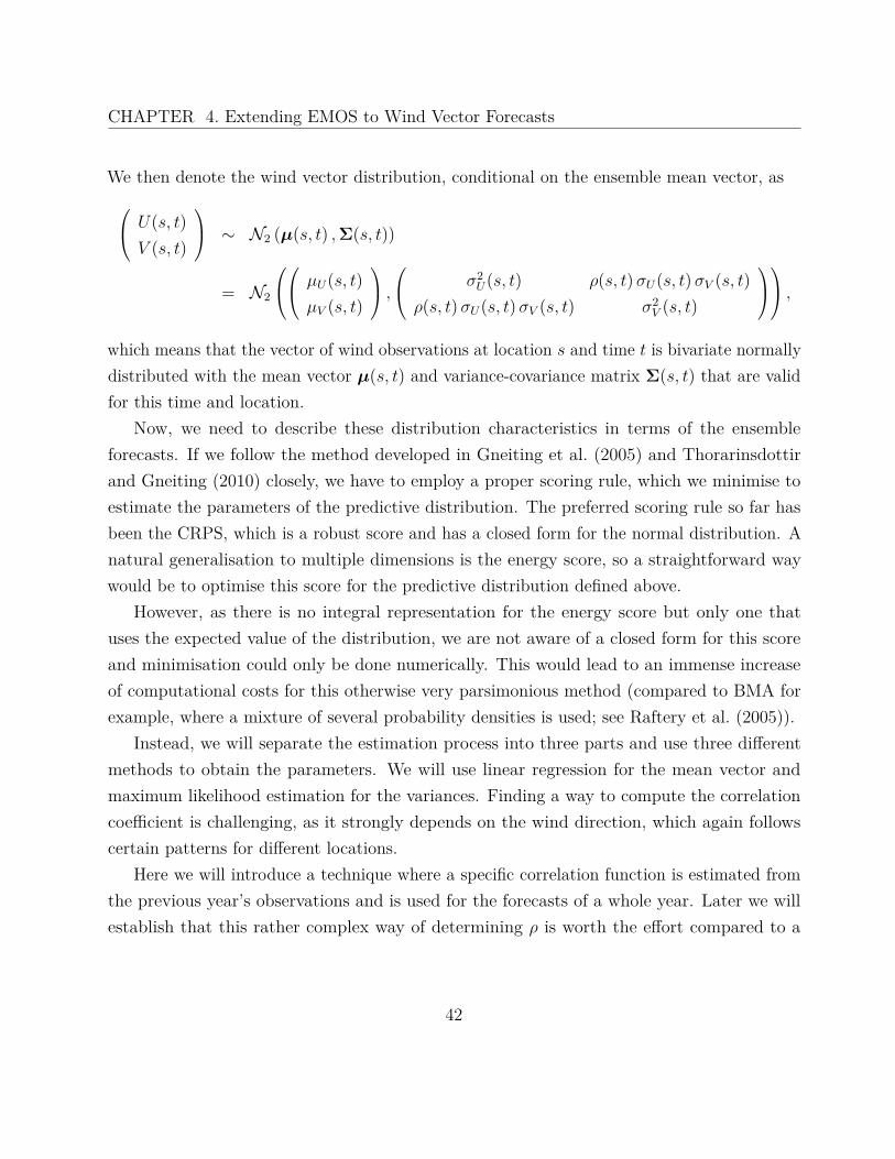
CHAPTER 4. Extending EMOS to Wind Vector Forecasts
We then denote the wind vector distribution, conditional on the ensemble mean vector, as
U(s, t)V (s, t)
∼ N2 (µ(s, t) , Σ(s, t))
= N2
µU(s, t)µV (s, t)
,
σ2U(s, t) ρ(s, t) σU(s, t) σV (s, t)
ρ(s, t) σU(s, t) σV (s, t) σ2V (s, t)
,
which means that the vector of wind observations at location s and time t is bivariate normallydistributed with the mean vector µ(s, t) and variance-covariance matrix Σ(s, t) that are validfor this time and location.
Now, we need to describe these distribution characteristics in terms of the ensembleforecasts. If we follow the method developed in Gneiting et al. (2005) and Thorarinsdottirand Gneiting (2010) closely, we have to employ a proper scoring rule, which we minimise toestimate the parameters of the predictive distribution. The preferred scoring rule so far hasbeen the CRPS, which is a robust score and has a closed form for the normal distribution. Anatural generalisation to multiple dimensions is the energy score, so a straightforward waywould be to optimise this score for the predictive distribution defined above.
However, as there is no integral representation for the energy score but only one thatuses the expected value of the distribution, we are not aware of a closed form for this scoreand minimisation could only be done numerically. This would lead to an immense increaseof computational costs for this otherwise very parsimonious method (compared to BMA forexample, where a mixture of several probability densities is used; see Raftery et al. (2005)).
Instead, we will separate the estimation process into three parts and use three differentmethods to obtain the parameters. We will use linear regression for the mean vector andmaximum likelihood estimation for the variances. Finding a way to compute the correlationcoefficient is challenging, as it strongly depends on the wind direction, which again followscertain patterns for different locations.
Here we will introduce a technique where a specific correlation function is estimated fromthe previous year’s observations and is used for the forecasts of a whole year. Later we willestablish that this rather complex way of determining ρ is worth the effort compared to a
42

CHAPTER 4. Extending EMOS to Wind Vector Forecasts
naive approach where we estimate the two wind components separately with no correlation atall (Section 5.3.3).
The eventual parameter estimation will therefore be executed following these three steps:
1. Estimate the predictive means by performing linear regressionon the ensemble means.
2. Compute the predictive correlation of the wind componentswith help of the previously estimated correlation function andthe predictive ensemble means from the first step.
3. Insert the results from steps 1 and 2 into the log-likelihood func-tion for the predictive distribution and estimate the remainingvariances.
In the following sections, the modelling of the predictive distribution characteristics and thedifferent ways of estimation will be presented.
4.2.3 The Mean Vector and Linear Regression
The analysis of the UWME data yielded that the distribution of wind vector observationsconditional on the ensemble mean is approximately bivariate normal. Therefore we suggestthe ensemble mean as sole predictor for the EMOS mean, in order to reduce the numberof parameters to estimate and to avoid a possible overparameterisation. Of course, thissupposition again only holds for ensembles with exchangeable members, which is not the casefor the UWME. This will be discussed further in Section 5.2.1.1 and we will examine if a
Table 4.1: Estimated parameters for the predictive mean at station KSEAvalid on 23 January 2008
aU bU aV bV
−0.69 0.86 −0.42 1.08
43

CHAPTER 4. Extending EMOS to Wind Vector Forecasts
●● ●●
●
●●
●
●
●
●
●
●
●
●
●
●
●
●
●
●
●
●
●
●●●
●
●
●
●●
●
●
●●
●
●●
●
−5 0 5 10
−50
510
(a)
ensemble mean
obse
rvat
ion
●
●
●
●
● ●
●●
●
●
●
●
●
●●
●
●
●
●●
●
●
● ●
●
●
●
●
●
●
●
●
●●
●
●
●
●●
●
−5 0 5 10−5
05
10
(b)
ensemble mean
obse
rvat
ion
Figure 4.5: Parameter estimation of the predictive mean vector for the 48-hour-aheadforecasts at Sea-Tac Airport, valid on 23 January 2008; pictured are the scatterplots of theensemble means and the verifying observations contained in the training data set, as well asthe respective fitted linear functions, for (a) the U component and (b) the V component
model using multiple linear regression with the initial ensemble forecasts as predictors showsbetter results for this ensemble.
So, with respect to the univariate method, we write the predictive means as linear functionsof the ensemble means U(s, t) = 1
M
�Mi=1 Ui(s, t) and V (s, t) = 1
M
�Mi=1 Vi(s, t):
µU(s, t) = aU + bU · U(s, t)µV (s, t) = aV + bV · V (s, t) .
Because only the four parameters aU , aV , bU , and bV (valid at station s and time t) aredetermined in this step, the best way to do so is using standard linear regression, for eachcomponent separately. Therefore we assume that we have a linear relationship between the
44
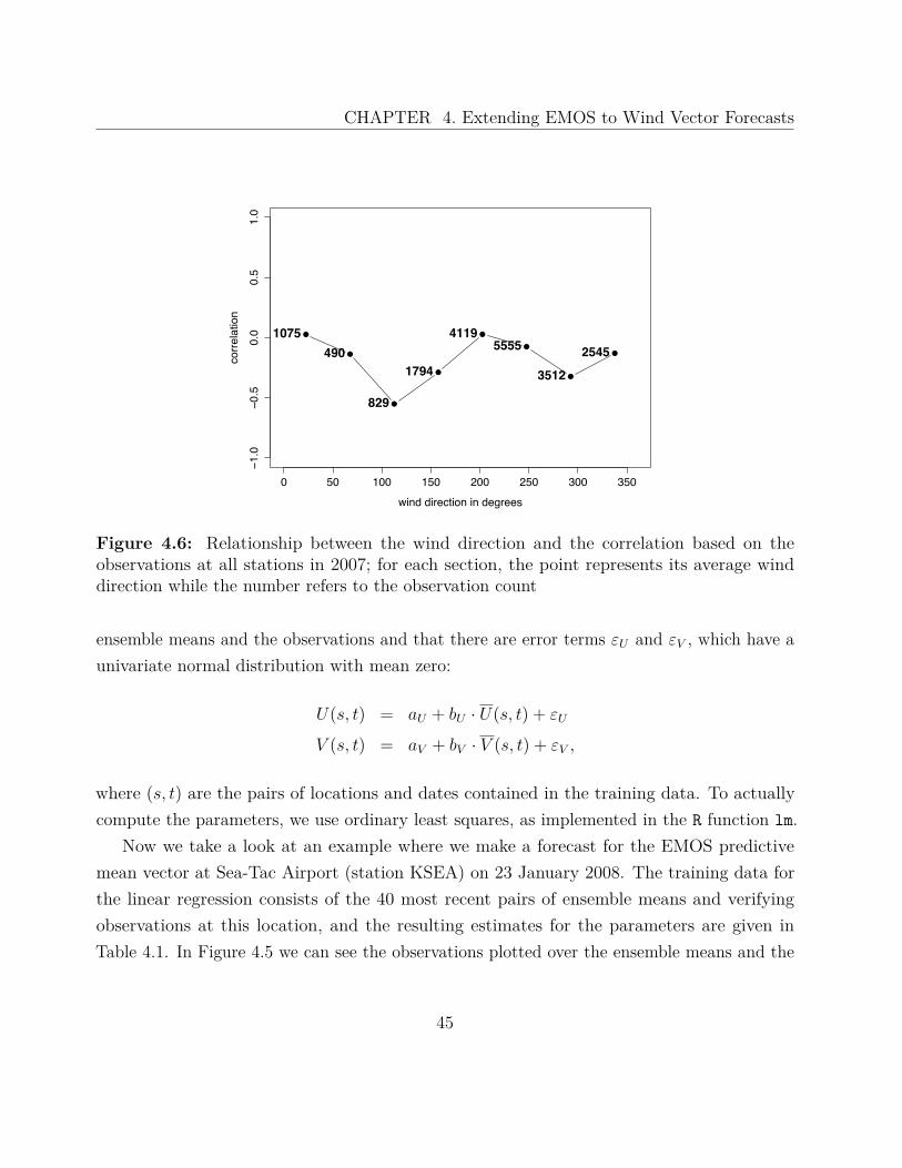
CHAPTER 4. Extending EMOS to Wind Vector Forecasts
●
●
●
●
●
●
●
●
0 50 100 150 200 250 300 350
−1.0
−0.5
0.0
0.5
1.0
wind direction in degrees
corre
latio
n
1075490
829
1794
41195555
3512
2545
Figure 4.6: Relationship between the wind direction and the correlation based on theobservations at all stations in 2007; for each section, the point represents its average winddirection while the number refers to the observation count
ensemble means and the observations and that there are error terms εU and εV , which have aunivariate normal distribution with mean zero:
U(s, t) = aU + bU · U(s, t) + εU
V (s, t) = aV + bV · V (s, t) + εV ,
where (s, t) are the pairs of locations and dates contained in the training data. To actuallycompute the parameters, we use ordinary least squares, as implemented in the R function lm.
Now we take a look at an example where we make a forecast for the EMOS predictivemean vector at Sea-Tac Airport (station KSEA) on 23 January 2008. The training data forthe linear regression consists of the 40 most recent pairs of ensemble means and verifyingobservations at this location, and the resulting estimates for the parameters are given inTable 4.1. In Figure 4.5 we can see the observations plotted over the ensemble means and the
45

CHAPTER 4. Extending EMOS to Wind Vector Forecasts
●● ●
●
●
●
●
●
0 50 100 150 200 250 300 350
−1.0
−0.5
0.0
0.5
1.0
wind direction in degrees
corre
latio
n
24 1 1
5
9748
1
39
Figure 4.7: Relationship between the wind direction and the correlation based on theobservations at station KSEA in 2007; for each section, the point represents its average winddirection while the number refers to the observation count
respective fitted linear functions. The ensemble mean vector for this day is (0.51, −0.01)T , sothe parameter estimation results in the predictive mean vector (−0.25, −0.44)T .
4.2.4 The Correlation Coefficient and the Wind Direction
Our next step in the estimation process is to develop a method in order to model the correlationcoefficient of the predictive normal distribution. In Section 4.2.1, we looked at scatter plots ofwind vector observations in different sections of the two-dimensional plane and establishedthat there seems to be a substantial correlation in several of them. This suggests that there isa strong connection between the direction of the forecast mean vector and the correlation ofthe two observation components U and V .
Further analysis of the data (Figures 4.6 and 4.7) will yield that the correlation in factchanges with a period of about 180°. The data used for this analysis is from 2007; we willalso use it for the estimation of the correlation curve. For Figure 4.6, the correlation between
46

CHAPTER 4. Extending EMOS to Wind Vector Forecasts
the observations for eight of the nine sections was computed and then plotted against therespective wind direction, with the numbers referring to the actual observation count in eachsection. We will not use section 1, the circle around zero, as it can not be associated with onesingle direction.
To obtain the actual predictive wind direction θ (in degrees) from the mean vectorcomponents µU and µV (as in Figure 4.1), the two-argument arctangent function is employed:
θ = 360°2π
· atan2 (−µU , −µV )
= 360°2π
·
arctan µUµV
µV < 0
arctan µUµV
+ π µU ≤ 0, µV > 0
arctan µUµV
− π µU > 0, µV < 0π2 µU < 0, µV = 0
−π2 µU > 0, µV = 0
0 µU = µV = 0.
As this function ranges from −180° to 180°, we add 360° to negative values and therefore getresults between 0° and 360°.
The shape of the resulting curve resembles that of a trigonometric function, so we canmake a first guess for modelling the correlation. A cosine function with four parameters seemsreasonable:
ρ(s, t) = r · cos (k · θ(s, t) + ϕ) + p,
where θ(s, t) is the wind direction of the predictive mean vector obtained in step 1. We have toconstrain the period to be an integer so that the consistency between the values at e.g. 0° and360° is retained, thus k has to be an integral multiple of 2π
360° . Figure 4.6 suggests k = 2 · 2π360° .
Furthermore, considering the same plot but with data from only one station, Figure 4.7 showsthat the wind direction/correlation relationship can vary locally. Due to lack of data, thisstation-specific curve however potentially changes over time.
An appropriate way to estimate the parameters r, ϕ, and p is non-linear least squaresregression, while k has to be determined empirically because of the constraint mentioned
47

CHAPTER 4. Extending EMOS to Wind Vector Forecasts
●
●
●
●
●
●
●
●
0 50 100 150 200 250 300 350
−1.0
−0.5
0.0
0.5
1.0
wind direction in degrees
corre
latio
n
1075490
829
1794
41195555
3512
2545
Figure 4.8: Empirical (solid line) and estimated (dashed line) correlation functions, basedon all available observations in the Pacific Northwest in 2007
above. A special wind pattern at a certain location can cause few or no observations in asection, resulting in correlations of 1 or −1. The number of observations in each section willserve as weights, therefore taking account of this unreasonable extremal values when there isonly little data available for a certain direction.
So, for estimating this trigonometric correlation function, we use the built-in R functionnls with the relative frequency of observations as weights. If we use the data from all stations,we get
ρ(s, t) = 0.20 · cos� 4π
360° · θ(s, t) − 1.08�
− 0.15,
which is shown in Figure 4.8. For the example where data from only one station is used, theweighted regression yields the curve in Figure 4.9; we chose a period of 360°, that is k = 2π
360° .The individual empirical and estimated correlation curves for all 79 stations and the respectivechoices for the parameter k can be found in Appendix A.
With this function we have found a way to describe and measure the relationship betweenthe wind direction and the correlation of the predictive distribution. It was established earlier
48

CHAPTER 4. Extending EMOS to Wind Vector Forecasts
●● ●
●
●
●
●
●
0 50 100 150 200 250 300 350
−1.0
−0.5
0.0
0.5
1.0
wind direction in degrees
corre
latio
n
24 1 1
5
9748
1
39
Figure 4.9: Empirical (solid line) and estimated (dashed line) correlation functions, basedon all available observations at Sea-Tac Airport in 2007
that the specific wind patterns don’t seem to vary much from year to year, so that we willuse the curves estimated with the 2007 data for issuing out-of-sample predictions in 2008. Incontinuing the example from the previous section, we take the bias-corrected predictive mean(−0.25, −0.44)T , compute the predicted wind direction θ = 30.24° and with this the predictivecorrelation ρ = 0.07. Here we use the location-specific correlation function for Sea-Tac Airport.
This brings the characterization of step 2 of the parameter estimation to an end, all thatremains is to employ the maximum likelihood technique and estimate the predictive variancesσ2
U and σ2V .
4.2.5 The Variances and Maximum Likelihood
In this section, we return to the conventional EMOS method and optimise a proper scoringrule to estimate the remaining parameters. Also, we want to model the predictive variances σ2
U
and σ2V as affine functions of the ensemble variances according to the one-dimensional variant:
49
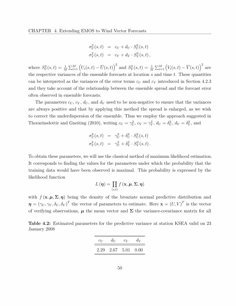
CHAPTER 4. Extending EMOS to Wind Vector Forecasts
σ2U(s, t) = cU + dU · S2
U(s, t)σ2
V (s, t) = cV + dV · S2V (s, t) ,
where S2U(s, t) = 1
M
�Mi=1
�Ui(s, t) − U(s, t)
�2and S2
V (s, t) = 1M
�Mi=1
�Vi(s, t) − V (s, t)
�2are
the respective variances of the ensemble forecasts at location s and time t. These quantitiescan be interpreted as the variances of the error terms εU and εV introduced in Section 4.2.3and they take account of the relationship between the ensemble spread and the forecast erroroften observed in ensemble forecasts.
The parameters cU , cV , dU , and dV need to be non-negative to ensure that the variancesare always positive and that by applying this method the spread is enlarged, as we wishto correct the underdispersion of the ensemble. Thus we employ the approach suggested inThorarinsdottir and Gneiting (2010), writing cU = γ2
U , cV = γ2V , dU = δ2
U , dV = δ2V , and
σ2U(s, t) = γ2
U + δ2U · S2
U(s, t)σ2
V (s, t) = γ2V + δ2
V · S2V (s, t) .
To obtain these parameters, we will use the classical method of maximum likelihood estimation.It corresponds to finding the values for the parameters under which the probability that thetraining data would have been observed is maximal. This probability is expressed by thelikelihood function
L (η) =�
(s,t)f (x, µ, Σ, η)
with f (x, µ, Σ, η) being the density of the bivariate normal predictive distribution andη = (γU , γV , δU , δV )T the vector of parameters to estimate. Here x = (U, V )T is the vectorof verifying observations, µ the mean vector and Σ the variance-covariance matrix for all
Table 4.2: Estimated parameters for the predictive variance at station KSEA valid on 23January 2008
cU dU cV dV
2.29 2.67 5.01 0.00
50

CHAPTER 4. Extending EMOS to Wind Vector Forecasts
forecasts contained in the training set (s, t). In practice it is often easier to maximise thelogarithm of the likelihood function, the log-likelihood function l (η), for reasons of algebraicsimplicity and numerical stability (Raftery et al. 2005). Thus our function to optimise becomes
l (η) = log
�
(s,t)f (x, µ, Σ, η)
= log
�
(s,t)
12π
√det Σ
· exp�
−12 (x − µ)T Σ (x − µ)
�
=�
(s,t)log
�1
2π√
det Σ· exp
�−1
2 (x − µ)T Σ (x − µ)��
=�
(s,t)
�
log�
12π
√det Σ
�
− 12 (x − µ)T Σ (x − µ)
�
=�
(s,t)
log
1
2π�
σ2Uσ2
V (1 − ρ2)
− 12
U − µU
V − µV
T
σ2U ρσUσV
ρσUσV σ2V
U − µU
V − µV
=�
(s,t)
log
1
2π�
γ2U + δ2
U · S2U(s, t)
�γ2
V + δ2V · S2
V (s, t)�
1 − ρ2(s, t)
− [U(s, t) − µU(s, t)]2
2 [1 − ρ2(s, t)] [γ2U + δ2
U · S2U(s, t)]
− [V (s, t) − µV (s, t)]2
2 [1 − ρ2(s, t)] [γ2V + δ2
V · S2V (s, t)]
+ ρ(s, t) [U(s, t) − µU(s, t)] [V (s, t) − µV (s, t)][1 − ρ2(s, t)] [γ2
U + δ2U · S2
U(s, t)] [γ2V + δ2
V · S2V (s, t)]
.
The values of the mean vector and the correlation coefficient don’t depend on η and arepreviously computed in step 1 and step 2. Of course, this function can only be applied if weassume that the forecast errors are independent of time and location. This assumption usually
51

CHAPTER 4. Extending EMOS to Wind Vector Forecasts
doesn’t hold, but as in Raftery et al. (2005) and Gneiting et al. (2005), possible dependencieswon’t have a large effect on the predictions because we only make forecasts for one time andone location simultaneously.
The actual numerical maximisation is done with the optim function in R using the Broyden-Fletcher-Goldfarb-Shanno algorithm. Maximum likelihood estimation can be perceived asoptimising the ignorance score (compare Section 2.3), so this method is equivalent to optimisinga proper scoring rule, similar to the univariate case. As initial values for the algorithm, we usethe results of the previous day’s estimation. This method does not necessarily find a globalmaximum, but in this case we found the maximisation to be relatively insensitive to the choiceof starting values.
For our example, Sea-Tac Airport on 23 January 2008, the estimated variance parametersare shown in Table 4.2. The ensemble variances S2
U and S2V are 0.19 and 0.69, respectively, so
the estimation results are the predictive variances σ2U = 2.79 and σ2
V = 5.01. Larger valuesfor dU or dV represent a high spread-error correlation in the training data, whereas on dayswhere there seems to be no spread-error correlation at all, the corresponding values will bevery small or even zero, like for the V component in our example.
In this manner, we conclude the description of our new EMOS postprocessing method,which is applicable to wind vectors, and proposes a way to extend the usual parameterestimation to multiple dimensions. The major changes compared to the univariate case is thatwe split the process into three parts and estimate the correlation coefficient with a trigonometricfunction of the predicted wind direction. In Section 5.4 we will see that this procedure resultsin a better performance than other approaches such as error dressing, separate postprocessingfor the individual wind vector components or the Ensemble Copula Coupling approach, wherewe take account of the dependency structure of the ensemble.
52
Chapter 5
Case Study and PredictivePerformance
After developing a bivariate EMOS method in the previous chapter, we now analyse itsout-of-sample predictive performance by conducting a case study for wind vector forecastsover the North American Pacific Northwest. This particular ensemble prediction systemwas also used to test the skill of the univariate EMOS variants described in Chapter 3. Wecompare two-dimensional EMOS to the unprocessed ensemble and a number of other forecaststaking the form of ensembles or densities. They include a climatological forecast based onpast observations, an ensemble dressing technique adding past errors to the ensemble mean, acombination of univariate EMOS predictive distributions for the individual vector components,and a multivariate postprocessing method using copulas. Finally, we examine if the bivariatemethod also creates calibrated and sharp wind speed forecasts and we assess its performancerelative to the original EMOS method for wind speed.
5.1 The University of Washington Mesoscale EnsembleIn order to test the skill of the new EMOS postprocessing technique, we use data provided by theUWME ensemble (as described in Eckel and Mass (2005)), for the period between 1 January2008 and 31 December 2008. During this time the eight-member multianalysis ensemble
53
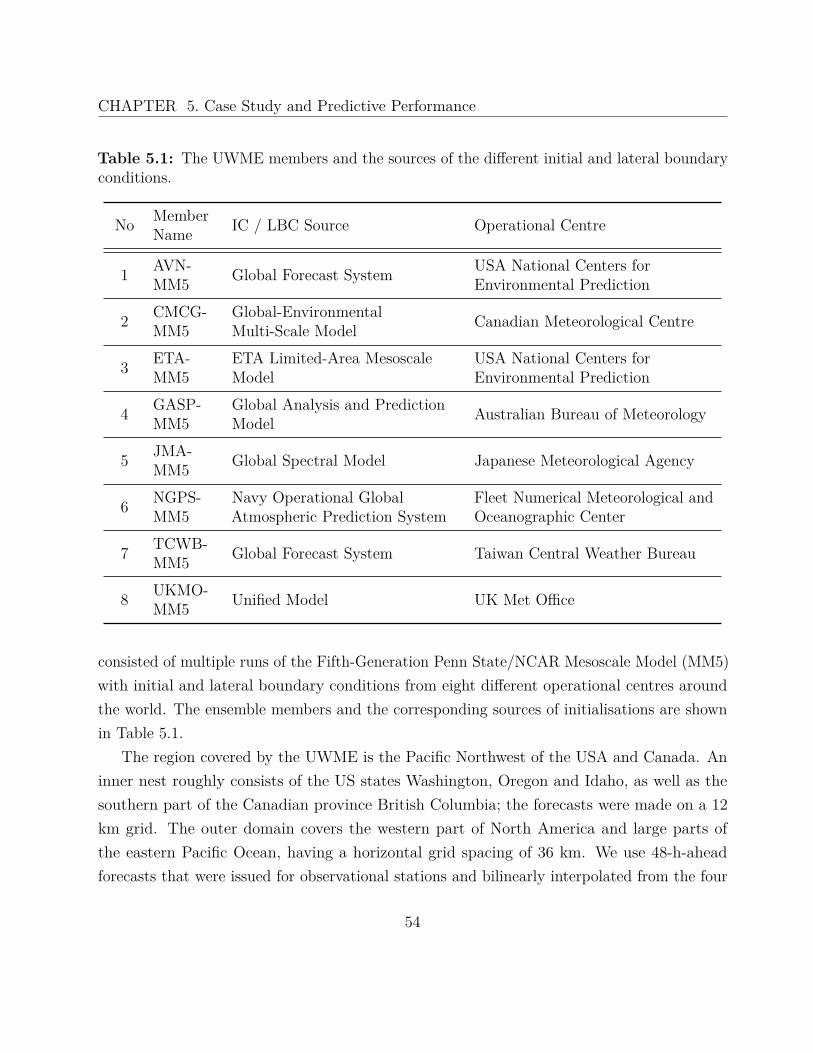
CHAPTER 5. Case Study and Predictive Performance
Table 5.1: The UWME members and the sources of the different initial and lateral boundaryconditions.
No MemberName IC / LBC Source Operational Centre
1 AVN-MM5 Global Forecast System USA National Centers for
Environmental Prediction
2 CMCG-MM5
Global-EnvironmentalMulti-Scale Model Canadian Meteorological Centre
3 ETA-MM5
ETA Limited-Area MesoscaleModel
USA National Centers forEnvironmental Prediction
4 GASP-MM5
Global Analysis and PredictionModel Australian Bureau of Meteorology
5 JMA-MM5 Global Spectral Model Japanese Meteorological Agency
6 NGPS-MM5
Navy Operational GlobalAtmospheric Prediction System
Fleet Numerical Meteorological andOceanographic Center
7 TCWB-MM5 Global Forecast System Taiwan Central Weather Bureau
8 UKMO-MM5 Unified Model UK Met Office
consisted of multiple runs of the Fifth-Generation Penn State/NCAR Mesoscale Model (MM5)with initial and lateral boundary conditions from eight different operational centres aroundthe world. The ensemble members and the corresponding sources of initialisations are shownin Table 5.1.
The region covered by the UWME is the Pacific Northwest of the USA and Canada. Aninner nest roughly consists of the US states Washington, Oregon and Idaho, as well as thesouthern part of the Canadian province British Columbia; the forecasts were made on a 12km grid. The outer domain covers the western part of North America and large parts ofthe eastern Pacific Ocean, having a horizontal grid spacing of 36 km. We use 48-h-aheadforecasts that were issued for observational stations and bilinearly interpolated from the four
54

CHAPTER 5. Case Study and Predictive Performance
surrounding grid points. Additionally, they were rotated to match the northern direction ateach station.
Observation data is provided by weather observation stations that are part of the AutomatedSurface Observing System network (National Weather Service 1998). Our new method isapplied to horizontal instantaneous surface wind, where “instantaneous” means that the windis measured and averaged over the last two minutes before the valid time at 00 UTC (see alsoGneiting et al. (2008), where a similar data set was used). To obtain verifying wind vectorobservations, the observed wind direction θ and wind speed w were transformed into vectors,using the following relationships (see Figure 4.1 for reference):
U = −w · sin� 2π
360° · θ�
V = −w · cos� 2π
360° · θ�
.
While being recorded in knots, the wind speed observations are rounded to the nearest wholeknot, and values below 1 knot are recorded as 0. Therefore the wind vector observations arediscretised, which is easily recognisable in Figures 4.3 and 4.4. Quality control procedures,described in Baars (2005), were applied, removing dates and locations with missing forecastsor observations from the data set.
For the time period considered, 19,282 pairs of ensemble forecasts and observations wereavailable, corresponding to 291 forecast days. There are 79 observation locations, whosedistribution is pictured in Figure 5.1. Additional data from the years 2006 and 2007 isrequired in order to provide an appropriate training period for all days of 2008, to estimatethe predictive correlation functions and to establish the optimal length of the rolling trainingperiods. Further information about the UWME, now using the WRF mesoscale model, aswell as real time forecasts and observations can be found at http://www.atmos.washington.edu/~ens/uwme.cgi.
55
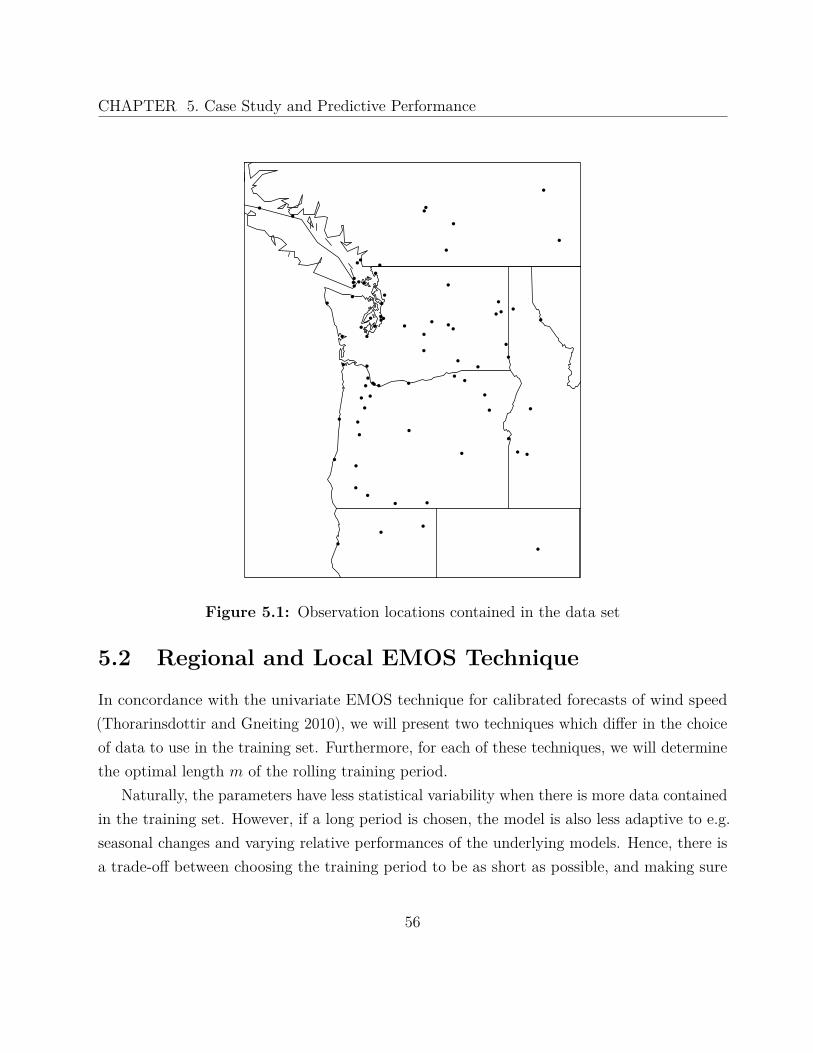
CHAPTER 5. Case Study and Predictive Performance
●
●
●
●
●
●
●
●
●
●
●●
●
●
●
●
●
●●
●
●
●
●
● ●
●
●
●
●
●
●
●
●
●
●
●
●
●
●
●
●
●
●
●●
●
●
●
●
●
●
●
●
●
●
●
●
●
●●
●
●
●
●
●
●●
●
●
●
●
●
●
●
●
●
●
●
●
Figure 5.1: Observation locations contained in the data set
5.2 Regional and Local EMOS TechniqueIn concordance with the univariate EMOS technique for calibrated forecasts of wind speed(Thorarinsdottir and Gneiting 2010), we will present two techniques which differ in the choiceof data to use in the training set. Furthermore, for each of these techniques, we will determinethe optimal length m of the rolling training period.
Naturally, the parameters have less statistical variability when there is more data containedin the training set. However, if a long period is chosen, the model is also less adaptive to e.g.seasonal changes and varying relative performances of the underlying models. Hence, there isa trade-off between choosing the training period to be as short as possible, and making sure
56

CHAPTER 5. Case Study and Predictive Performance
that, at the same time, calibrated and sharp predictive distributions are produced. To obtainthe best choice, we apply the bivariate EMOS method to data from the calendar year 2007,using additional data from 2006 to provide full training periods for all dates. This data isnot used for evaluating the performance of the new EMOS method. In this experiment, wecomputed the out-of-sample energy score and the Euclidean error, averaged over all datesand locations, considering various training period lengths. Therefore the optimal trainingperiod length is where these scores are minimised, as proper scoring rules assess calibrationand sharpness simultaneously.
5.2.1 Regional EMOS
For the regional EMOS technique, on each day only one set of parameters is estimated andused to produce forecast for all stations. The training set consists of all available data fromthe 79 stations and the last m days prior to the forecast being made. Should data be missingat certain dates or stations, these are omitted from the training set. For example, if we assumea training period length of 40 days, and make forecast for day 183, issued on day 181, allforecasts and observations from dates 142 to 181 are included in the training set. As for thecorrelation curve, all forecasts and observations of the previous calendar year, i.e. 2007, areemployed to estimate one correlation function (see Figure 4.8).
This technique allows us to produce forecasts for any location in our area of interestfor which ensemble forecasts are available, even if there should be no training data at thisparticular station. It also has the advantage of being very parsimonious, as only very fewparameters have to be computed. Thus we can think about extending the parameter estimationso that we make use of the ensemble forecasts themselves.
5.2.1.1 Using Multiple Linear Regression to Estimate the Predictive Mean
As suggested before (Section 4.2.3), we consider two different kinds of estimation for thepredictive mean. Initially only the ensemble mean was used as predictor for the linear regression.However, as the regional EMOS technique comes with a large amount of training data, itis possible to fit more parameters and we can also estimate the predictive mean as a linearfunction of the original ensemble member forecasts:
57

CHAPTER 5. Case Study and Predictive Performance
●●●●●
●
●
●●●●●●
●●●●●●●●●●●●●
●●●●
●
●●
●●●
●
●●●●●●●●●●●●●●●●●●●●
●●●●●●
●●●●●
●●●●●
●●
●●
●●●●●●●●●●●●●●●●●●●●●●●●●●●
●●●●●●●●●●●●●●
●
●
●
●●●●●●●●●●●●●●●●●●●●●●●●●●●●●●●●●●
●●
●●
●●●●●●●●
●
●●●●●●
●●●●●●●●●●●●●●●●●●●●●●●●●●●●●●●●●●●●●
●●●●
●●●●●●●●●●●
●●●●●
●
●
●
●●●●●●●●
●●●●●●●●●●●●●●●
●●
●●
●●
●
●●●●●●●●●●●
●●
●●●●●●●●●●●●●●
0 50 100 150 200 250 300
02
46
8
(a)
Day Index
Num
ber o
f Non−z
ero
Coe
ffici
ents
●
●
●
●
●●●●
●
●
●
●
●
●●●
●●●
●
●
●
●
●
●●
●
●
●●
●●●
●●●●●●●●
●
●●●●●●
●●
●
●●●●●●●●●●●●●●●●●●●●●●●●
●●●●
●●
●●
●
●
●
●●
●●●●●●●●●●●●●
●
●
●●●●●
●●●●●●●●●●●
●
●
●
●
●
●●
●
●
●●●
●●●●●
●●●●
●●
●
●●●●●●●●●●●●●●●●●●●●●●●●●●●●●●●
●
●
●●
●●●●
●●●●
●●●●●●●●●●●●●●
●
●
●●●
●●●
●
●●●●●●●●●●●●●
●●●●
●●●●●●●●●●
●●
●
●
●●
●●●●●
●●●
●●●●●●●●●
●●
●●●
●●●
●●●●●●
●●●●●●●●●
●●●●●●●●
●
0 50 100 150 200 250 3000
24
68
(b)
Day Index
Num
ber o
f Non−z
ero
Coe
ffici
ents
Figure 5.2: Number of non-zero EMOS+ coefficients when estimating the predictive meanfor all dates in the data set: (a) U wind component and (b) V wind component
µU(s, t) = aU + bU,1 · U1(s, t) + . . . + bU,8 · U8(s, t)µV (s, t) = aV + bV,1 · V1(s, t) + . . . + bV,8 · V8(s, t) .
Again, we obtain the parameters aU , bU,1, . . . , bU,8 and aV , bV,1, . . . , bV,8 by performing twoseparate linear regressions before the correlation coefficient and variances are estimated asusual. To improve interpretability, the coefficients bU,1, . . . , bU,8 and bV,1, . . . , bV,8 must benon-negative. In order to ensure this, we use a variant of the EMOS+ technique proposedby Gneiting et al. (2005). As the coefficients are estimated using a linear regression model,we proceed the following way. After determining the regular regression estimates, we removethose ensemble members with non-negative parameters from the training set and set theircoefficients to zero, then estimate again. This is repeated until there are only non-negativecoefficients left. For the remainder of the parameter estimation, i.e. the computing of thepredictive correlation and the maximum likelihood estimation, we use the ensemble variance
58
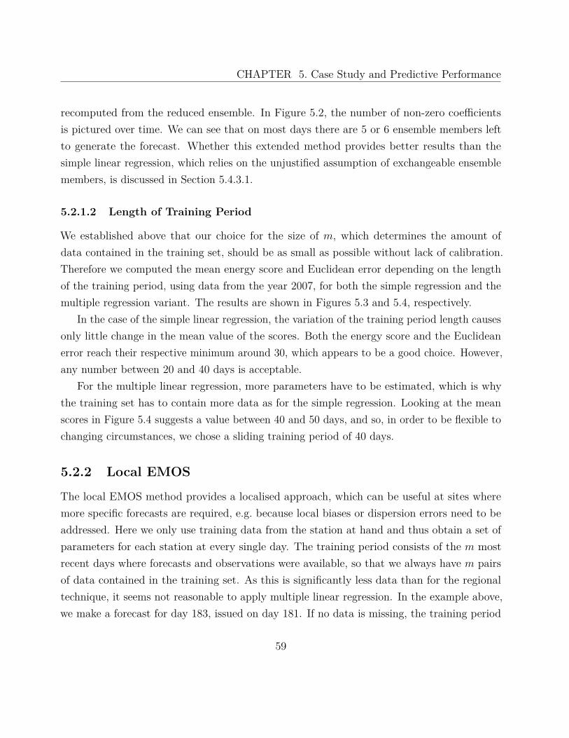
CHAPTER 5. Case Study and Predictive Performance
recomputed from the reduced ensemble. In Figure 5.2, the number of non-zero coefficientsis pictured over time. We can see that on most days there are 5 or 6 ensemble members leftto generate the forecast. Whether this extended method provides better results than thesimple linear regression, which relies on the unjustified assumption of exchangeable ensemblemembers, is discussed in Section 5.4.3.1.
5.2.1.2 Length of Training Period
We established above that our choice for the size of m, which determines the amount ofdata contained in the training set, should be as small as possible without lack of calibration.Therefore we computed the mean energy score and Euclidean error depending on the lengthof the training period, using data from the year 2007, for both the simple regression and themultiple regression variant. The results are shown in Figures 5.3 and 5.4, respectively.
In the case of the simple linear regression, the variation of the training period length causesonly little change in the mean value of the scores. Both the energy score and the Euclideanerror reach their respective minimum around 30, which appears to be a good choice. However,any number between 20 and 40 days is acceptable.
For the multiple linear regression, more parameters have to be estimated, which is whythe training set has to contain more data as for the simple regression. Looking at the meanscores in Figure 5.4 suggests a value between 40 and 50 days, and so, in order to be flexible tochanging circumstances, we chose a sliding training period of 40 days.
5.2.2 Local EMOS
The local EMOS method provides a localised approach, which can be useful at sites wheremore specific forecasts are required, e.g. because local biases or dispersion errors need to beaddressed. Here we only use training data from the station at hand and thus obtain a set ofparameters for each station at every single day. The training period consists of the m mostrecent days where forecasts and observations were available, so that we always have m pairsof data contained in the training set. As this is significantly less data than for the regionaltechnique, it seems not reasonable to apply multiple linear regression. In the example above,we make a forecast for day 183, issued on day 181. If no data is missing, the training period
59
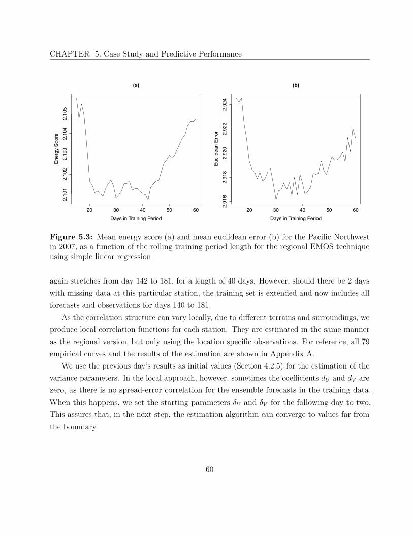
CHAPTER 5. Case Study and Predictive Performance
20 30 40 50 60
2.10
12.
102
2.10
32.
104
2.10
5
(a)
Days in Training Period
Ener
gy S
core
20 30 40 50 60
2.91
62.
918
2.92
02.
922
2.92
4
(b)
Days in Training PeriodEu
clid
ean
Erro
r
Figure 5.3: Mean energy score (a) and mean euclidean error (b) for the Pacific Northwestin 2007, as a function of the rolling training period length for the regional EMOS techniqueusing simple linear regression
again stretches from day 142 to 181, for a length of 40 days. However, should there be 2 dayswith missing data at this particular station, the training set is extended and now includes allforecasts and observations for days 140 to 181.
As the correlation structure can vary locally, due to different terrains and surroundings, weproduce local correlation functions for each station. They are estimated in the same manneras the regional version, but only using the location specific observations. For reference, all 79empirical curves and the results of the estimation are shown in Appendix A.
We use the previous day’s results as initial values (Section 4.2.5) for the estimation of thevariance parameters. In the local approach, however, sometimes the coefficients dU and dV arezero, as there is no spread-error correlation for the ensemble forecasts in the training data.When this happens, we set the starting parameters δU and δV for the following day to two.This assures that, in the next step, the estimation algorithm can converge to values far fromthe boundary.
60
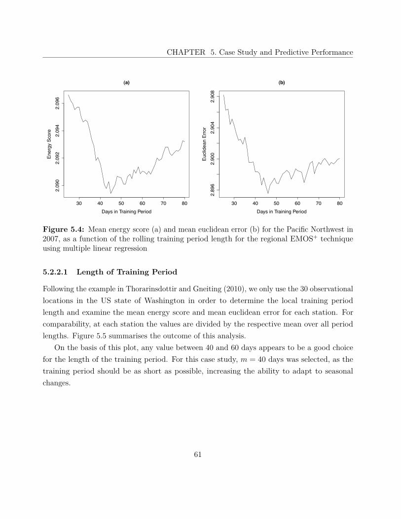
CHAPTER 5. Case Study and Predictive Performance
30 40 50 60 70 80
2.09
02.
092
2.09
42.
096
(a)
Days in Training Period
Ener
gy S
core
30 40 50 60 70 80
2.89
62.
900
2.90
42.
908
(b)
Days in Training PeriodEu
clid
ean
Erro
r
Figure 5.4: Mean energy score (a) and mean euclidean error (b) for the Pacific Northwest in2007, as a function of the rolling training period length for the regional EMOS+ techniqueusing multiple linear regression
5.2.2.1 Length of Training Period
Following the example in Thorarinsdottir and Gneiting (2010), we only use the 30 observationallocations in the US state of Washington in order to determine the local training periodlength and examine the mean energy score and mean euclidean error for each station. Forcomparability, at each station the values are divided by the respective mean over all periodlengths. Figure 5.5 summarises the outcome of this analysis.
On the basis of this plot, any value between 40 and 60 days appears to be a good choicefor the length of the training period. For this case study, m = 40 days was selected, as thetraining period should be as short as possible, increasing the ability to adapt to seasonalchanges.
61
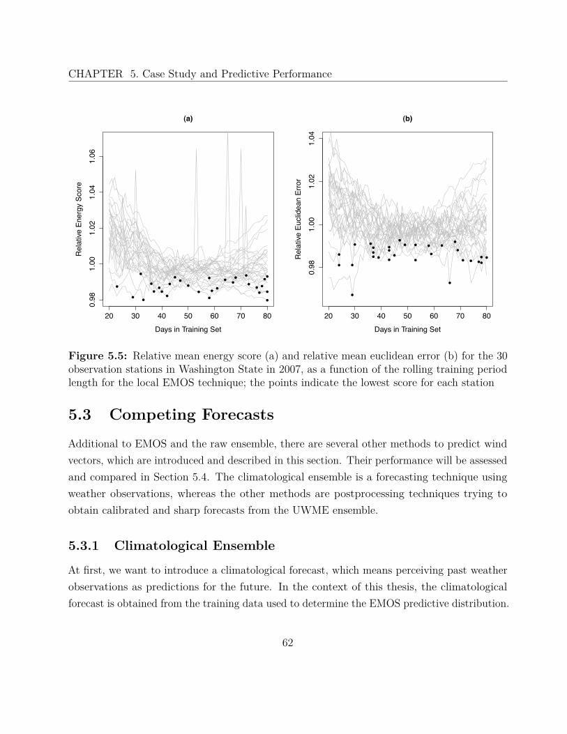
CHAPTER 5. Case Study and Predictive Performance
20 30 40 50 60 70 80
0.98
1.00
1.02
1.04
1.06
(a)
Days in Training Set
Rel
ative
Ene
rgy
Scor
e
●●
●●●
●
●
●
●
●
●
●● ●●
●
●●
●
●
● ●
●
●
● ●●
●
●
●
20 30 40 50 60 70 800.
981.
001.
021.
04
(b)
Days in Training Set
Rel
ative
Euc
lidea
n Er
ror
● ●
●
●●
●
●
●
●
●
●●
●
●●
●
●●
●
●
●
●●
●
●●
●
●
●
●
Figure 5.5: Relative mean energy score (a) and relative mean euclidean error (b) for the 30observation stations in Washington State in 2007, as a function of the rolling training periodlength for the local EMOS technique; the points indicate the lowest score for each station
5.3 Competing ForecastsAdditional to EMOS and the raw ensemble, there are several other methods to predict windvectors, which are introduced and described in this section. Their performance will be assessedand compared in Section 5.4. The climatological ensemble is a forecasting technique usingweather observations, whereas the other methods are postprocessing techniques trying toobtain calibrated and sharp forecasts from the UWME ensemble.
5.3.1 Climatological Ensemble
At first, we want to introduce a climatological forecast, which means perceiving past weatherobservations as predictions for the future. In the context of this thesis, the climatologicalforecast is obtained from the training data used to determine the EMOS predictive distribution.
62

CHAPTER 5. Case Study and Predictive Performance
From the wind vector observations contained in this data, m vectors are randomly sampled,yielding an ensemble of the same size as the length of the EMOS rolling training period. Againwe have a regional and a local technique, so that all forecasting methods can be compareddirectly. The regional technique uses observations from all locations available, and the localonly from the station at hand.
As the observations are rounded and include many values equaling zero, the ensemble sizeis larger as compared to the UWME to avoid numerical problems on one hand and to improvethe fitting of a normal distribution (as described in Section 5.3.5) on the other.
5.3.2 Error Dressing Ensemble
In Gneiting et al. (2008), a postprocessing method called error dressing was discussed, producingwell-performing forecasts. It uses the raw ensemble’s own statistical errors to generate anew ensemble that is corrected for biases and dispersion errors. The general approach wasfirst proposed in Roulston and Smith (2003), where it is called “dressing” and applied toeach member of the ensemble. Here we will content ourselves with creating an error dressingensemble from the UWME mean forecast and the corresponding verifying observation. Thedata used are again the respective training sets for the regional and local EMOS methods.
First we compute the ensemble mean errors,
eU(s, t)eV (s, t)
=
U(s, t) − U(s, t)V (s, t) − V (s, t)
,
where (s, t) ranges over all stations and dates contained in the training data set. From this
empirical error distribution, m errors
eU,1, . . . , eU,m
eV,1, . . . , eV,m
are sampled and then added to the
UWME mean for the current forecast day and location. This results in the new error dressingensemble with m ensemble members:
U + eU,1
V + eV,1
, . . . ,
U + eU,m
V + eV,m
.
63

CHAPTER 5. Case Study and Predictive Performance
In contrast to Gneiting et al. (2008), we only make use of past errors to simplify compara-bility of all postprocessing and forecasting methods. For the same reason, both regional andlocal forecasts are provided.
5.3.3 EMOS for Wind Vector Components
As the wind vector data is given in form of its meridional and longitudinal components, the ideacomes to mind that the conventional one-dimensional EMOS method could be applied to thetwo components separately. Recall that in Section 4.2.1 it was established that wind vectorsseem to be normally distributed. Therefore, the resulting univariate predictive distributionscan be joined to a bivariate normal distribution, assuming that U and V are independent andhence especially are not correlated.
To propose such an approach, we can follow the method as it was described in Gneitinget al. (2005) and Section 3.2 and model the predictive distribution of a wind component Y atlocation s and time t, conditional on ensemble forecasts X1, . . . , XM , accordingly:
Y (s, t) | X1(s, t) , . . . XM(s, t) ∼ N�µ(s, t) , σ2(s, t)
�.
The EMOS mean µ is a linear function of the ensemble members,
µ(s, t) = a + b1X1(s, t) + . . . + bMXM(s, t) ,
and the predictive variance σ2 an affine function of the ensemble variance S2,
σ2(s, t) = c + d · S2(s, t) .
For the parameter estimation, we return to the method of CRPS minimisation and estimateall parameters simultaneously. The only difference compared to Gneiting et al. (2005) isthat we do not use the method introduced as EMOS+ to ensure non-negative values forb1, . . . , bM , but rather the one by Thorarinsdottir and Gneiting (2010), where these coefficientsare written as β2
1 , . . . , β2M , additional to c = γ2 and d = δ2. Then the estimation is performed,
unconstrained, over a, β1, . . . , βM , γ, and δ.
64
CHAPTER 5. Case Study and Predictive Performance
After the described method is applied to both U and V forecasts, we combine the results,namely µU , µV , σ2
U , and σ2V , to obtain a bivariate probability distribution:
U(s, t)V (s, t)
∼ N2
µU(s, t)µV (s, t)
,
σ2U(s, t) 0
0 σ2V (s, t)
.
This distribution can be assessed in the same way as the one generated by the bivariatemethod taking the correlation into account. The comparison of these two distributions tellsus if a two-dimensional approach to wind vectors is justified at all, or if it suffices to addressthe vector components individually. As before, we produce regional as well as local forecasts,using the same length of training period as in Sections 5.2.1 and 5.2.2. In the following, thismethod is referred to as EMOSUV .
5.3.4 ECC Ensemble
The fourth technique we want to compare our EMOS method to, is called Ensemble CopulaCoupling (ECC). It was developed to combine already postprocessed forecasts, so that multipleweather quantities, locations or forecast horizons can be addressed together. In this manner,multivariate dependence structures are inherited from the ensemble. More information aboutECC can be found in Schefzik (2011).
In the current framework, we plan to apply this approach to the univariate EMOSUV
forecasts produced by the method described in the preceding section. Thus we obtain atwo-dimensional ensemble that takes account of the correlation structure between the windcomponents, instead of just assuming that they are independent.
We proceed as follows:
1. Employ univariate statistical postprocessing:At first, we apply the aforementioned EMOSUV postprocessing method forwind components to the ensemble forecasts U1, . . . , U8 and V1, . . . , V8. In thisway, we obtain calibrated and sharp univariate predictive distributions for U
and V .
65

CHAPTER 5. Case Study and Predictive Performance
2. Draw random samples:We draw samples U1, . . . , U8 and V1, . . . , V8 from the EMOSUV predictive dis-tributions of both U and V wind components. Here, random samples are used,as compared to equally spaced quantiles in Schefzik (2011).
3. Arrange according to the multivariate structure:In order to copy the multivariate structure of the ensemble, we determine theorder statistics of the unprocessed ensemble members for each wind compo-nent, where ties are resolved at random. By this procedure, our ensemblebecomes Uσ(1), . . . , Uσ(8) and Vµ(1), . . . , Vµ(8) with the respective order statisticsσ (1) , . . . , σ (8) and µ (1) , . . . , µ (8). Then the accordingly ordered samples
Uσ(1)
Vµ(1)
, . . . ,
Uσ(8)
Vµ(8)
constitute the ECC ensemble, which has inherited the dependence structure fromthe raw ensemble, although relying only on one-dimensional postprocessing.
In the general ECC approach, a sample of the magnitude of the ensemble size is generated andordered; we follow this in the computation of the Euclidean error, the determinant sharpnessand the multivariate rank histogram. For computing the energy score, however, a sample sizeof 10,000 is required (refer to Section 2.3.2). Thus we repeat the last two steps 1,250 times,thereby creating a total of 10,000 vectors.
5.3.5 Converting Ensemble and Density Forecasts
In order to compare all forecasts in this case study, we use the assessment tools introducedin Chapter 2. Some of the tools only apply to one form of probabilistic forecasts, eitherensembles or probability distributions. Therefore, we have to convert the forecasts to assesstheir performance with these methods.
Sampling from a predictive distribution yields a discrete ensemble of any desired size.Gneiting et al. (2005) proposed taking quantiles at levels i
M+1 , for i = 1, . . . , M . However,
66
CHAPTER 5. Case Study and Predictive Performance
bivariate quantiles are hard to determine, which is why we use random samples to obtain theensemble vectors.
For a given ensemble forecast, we replace it by a bivariate normal density estimate.The distribution characteristics are directly gained from the ensemble, with the ensemblemeans as mean vector, and the empirical ensemble variances and correlation generating thevariance-covariance matrix of the new full predictive distribution.
5.4 Predictive Performance for Wind Vector ForecastsAt this point, we begin describing the predictive performance of the new bivariate EMOSmethod as well as of the other forecasting and postprocessing techniques introduced in theprevious section. First, we recapture the example from Chapter 4, where we consideredforecasts for the 23 January 2008 at Sea-Tac Airport. Then the performance of the localtechniques at this station is discussed, by means of the forecasts for the calendar year 2008.Finally, we present our findings aggregated over all locations for both regional and localforecasts.
5.4.1 Results for Sea-Tac Airport, 23 January 2008
To illustrate EMOS in practice, we consider one date at one location, where we producelocal and regional postprocessed forecasts. In Chapter 4, it was explained how we obtainthe parameter estimates for the predictive distribution using linear regression for the meanvector, weighted non-linear regression for the correlation coefficient and maximum likelihoodestimation for the variances. This estimation procedure was conducted for predictions atSea-Tac Airport, valid on 23 January 2008.
Table 5.2 shows the parameter estimates for the local and the regional technique. Forcomparability reasons, we choose the regional EMOS forecast which uses simple linear regressionon the ensemble mean. Correspondingly, the characteristics of the predictive distributions,as well as the ensemble means, ensemble variances and verifying observation are specified inTable 5.3.
67

CHAPTER 5. Case Study and Predictive Performance
Table 5.2: Parameter estimates at station KSEA, valid on 23 January 2008, for the localand regional EMOS techniques both using simple linear regression
Method aU bU cU dU aV bV cV dV
local EMOS −0.69 0.86 2.29 2.67 −0.42 1.08 5.01 0.00regional EMOS −0.56 0.55 3.19 0.86 0.04 0.60 4.44 1.10
Table 5.3: Local and regional EMOS means, variances and correlation, as well as ensemblemeans, ensemble variances and the verifying observation for station KSEA, valid on 23 January2008
Method µU µV σ2U σ2
V ρ
local EMOS −0.25 −0.43 2.79 5.01 0.07regional EMOS −0.28 0.03 3.35 5.19 −0.29
U V S2U S2
V U V
0.51 −0.01 0.19 0.69 −1.34 0.77
Both methods roughly agree on the parameters for the predictive mean of the U component,while there is a significant difference in the other dimension. The local method suspects a largenegative bias for V , and therefore corrects the mean in the wrong direction. In the case of thevariance parameters, regional EMOS detects a relatively weak spread-skill relationship in bothdimensions, with dU and dV being around one. Using only the location-specific training dataeven yielded that, for V , ensemble spread and forecast error are not correlated at all, resultingin a large value for cV and a dV equalling zero. In this way, the variances of the underdispersiveensemble are substantially enlarged. Also, by means of the correlation estimates, one can seethe effects of using different predictive correlation functions for the two techniques.
Figures 5.6 and 5.7 let us compare the forecasts graphically. The regional EMOS mean isa better point forecast for the observation than the local EMOS mean. Their dispersion isvery similar, apart from the differing correlations. For the local method, the observation liesjust outside the 25% ellipse, while it lies well within for the regional method. Both plots show
68

CHAPTER 5. Case Study and Predictive Performance
−4 −2 0 2 4
−6−4
−20
24
U
V
90%
75%
50%
25%
●
●
●
●
●●
●
●
90%
Figure 5.6: Contour plot of the local EMOS and the UWME forecasts; the green, blue andred asterisks represent the EMOS mean, the ensemble mean and the verifying observation,respectively; the green ellipses are the 25%, 50%, 75% and 90% EMOS prediction ellipses,while the blue one is the 90% prediction ellipse of the fitted UWME distribution
clearly that the spread of the UWME is far too small, with the observation way outside of theensemble range and the 90% prediction ellipse.
When we visualise the predictive distributions with a perspective plot (Figures 5.8 and5.9), the underdispersion becomes even more obvious, as the fitted UWME density is muchmore concentrated. Additionally, in Figure 5.8, the observation is positioned near the centreof the density, whereas in Figure 5.9 it lies in the outer margins, indicating the skill of theEMOS mean as point forecast.
69

CHAPTER 5. Case Study and Predictive Performance
−4 −2 0 2 4
−6−4
−20
24
U
V
90%
75%
50%
25%
●
●
●
●
●●
●
●
90%
Figure 5.7: Contour plot of the regional EMOS and the UWME forecasts; the green, blueand red asterisks represent the EMOS mean, the ensemble mean and the verifying observation,respectively; the green ellipses are the 25%, 50%, 75% and 90% EMOS prediction ellipses,while the blue one is the 90% prediction ellipse of the fitted UWME distribution
Quantifying the performance using the energy score and the Euclidean error (Table 5.4),we find that, as expected, the regional method has the smallest scores, with local EMOS beingslightly higher. The UWME is by far the least skillful predictor, in terms of both probabilisticand deterministic forecasts.
70

CHAPTER 5. Case Study and Predictive Performance
Table 5.4: Energy score and Euclidean error for local EMOS, regional EMOS, and UWMEforecasts at station KSEA, valid on 23 January 2008
Method ES EE
Local EMOS 1.122 1.557Regional EMOS 1.008 1.269Raw ensemble 1.690 2.116
U
−4−2
0
2
4
6
V
−4−2
02
4
6
PDF0.01
0.02
0.03
0.04
●
Figure 5.8: Three-dimensional perspective plot of the local EMOS predictive density; thedot indicates the verifying observation
71
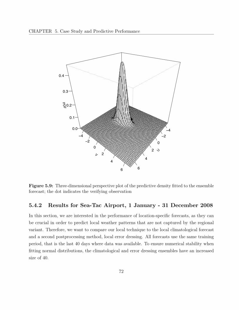
CHAPTER 5. Case Study and Predictive Performance
U
−4−2
0
2
4
6
V
−4−2
02
4
6PDF
0.0
0.1
0.2
0.3
0.4
●
Figure 5.9: Three-dimensional perspective plot of the predictive density fitted to the ensembleforecast; the dot indicates the verifying observation
5.4.2 Results for Sea-Tac Airport, 1 January - 31 December 2008
In this section, we are interested in the performance of location-specific forecasts, as they canbe crucial in order to predict local weather patterns that are not captured by the regionalvariant. Therefore, we want to compare our local technique to the local climatological forecastand a second postprocessing method, local error dressing. All forecasts use the same trainingperiod, that is the last 40 days where data was available. To ensure numerical stability whenfitting normal distributions, the climatological and error dressing ensembles have an increasedsize of 40.
72

CHAPTER 5. Case Study and Predictive Performance
● ● ● ● ● ●●
● ● ●●●●●●●● ●●●● ●● ●●●●● ●●●●●●● ●● ●● ● ●●●● ●●●●●● ● ●
●● ●● ●●●●●● ●● ●● ● ●●● ●●●● ● ●● ●●●●
● ●●● ● ●● ● ●● ●●● ●● ●●●● ●●● ● ● ●●●●● ●● ●●●●●●●●● ●●●●●● ●●● ●●●●●●● ● ● ●● ● ●●●●● ● ●● ● ● ● ● ●● ● ●●● ●●●●●● ●● ●●● ● ● ●● ● ●● ●● ●● ●● ● ●● ●● ●●●●●●●● ● ● ●● ● ● ● ● ●●●
● ● ●●●● ● ● ● ● ● ● ● ●● ● ●● ●● ● ● ●● ● ● ● ● ● ● ● ● ● ●●
● ● ● ●● ●● ● ● ●● ● ●●●●
●●●●● ●● ●●● ● ● ● ● ● ● ● ●● ●●●
050
100
150
200
250
−1012
(a)
Dai
ly In
dex
aU
●●●● ●●●
●●●●● ●● ● ● ● ● ●● ●●●● ● ●●●●● ● ● ●●●● ● ●● ●● ● ● ●● ● ●● ●● ● ●● ●●
●● ● ● ●● ●● ●● ●
●●●● ●●● ●●●● ● ● ●●●● ● ●●● ●●● ●● ● ●● ●● ● ● ●● ● ● ●●●● ● ● ●● ●● ● ● ● ●●●● ●● ●● ● ● ●● ●● ●●● ● ● ● ●● ●● ●●●● ● ● ● ●● ●●●●●● ●
●● ● ●● ● ● ● ●●● ●● ● ●●● ● ●●● ●● ●●
●● ●●● ●● ●● ● ● ● ● ● ●●
●●● ● ●●●●●● ● ●●● ● ● ●
●●●●●●●● ●●●● ● ● ●●●●●●● ●● ●●● ●●● ●● ●●● ● ●● ●●●●● ●●● ●● ● ●● ●●
●●● ●● ● ●●●● ●● ● ●●
050
100
150
200
250
0.00.51.01.5
(b)
Dai
ly In
dex
bU
● ●●● ●●●● ●● ●● ● ● ●●● ●●●●●●●●●●●● ●● ● ● ● ●● ●● ● ●● ● ●● ●●●● ●●● ● ● ●●
● ●● ●●● ●● ● ● ●●●● ●●●● ●●● ●● ●●●● ● ● ● ● ●●●●
● ●●●●●● ●●●●●
●●●● ● ● ● ● ●● ●● ● ● ● ● ● ● ● ● ● ●●● ●● ● ● ● ● ●●●● ●● ● ● ●● ● ●●● ●●●●● ● ●● ● ●● ●●● ● ●●●●●● ● ●●●●●●●●● ●● ●●
●●● ● ●●● ● ● ● ● ● ● ● ● ●● ●● ●●●●●●● ● ●● ●●● ● ●●●●●●● ● ● ●● ● ●●●●●● ●
● ● ● ●● ●●●●● ● ●●● ●●●●● ● ● ●● ● ● ● ● ● ● ●●●●
● ● ● ●●
●●●●●●● ● ● ●
050
100
150
200
250
246
(c)
Dai
ly In
dex
cU
●● ● ● ● ●●●● ●● ●●●● ● ●● ●● ● ● ●●● ● ● ● ● ●●●●●● ●● ●●● ● ●● ●●● ● ● ● ● ●●●●●●● ●●●●● ●●●●● ● ●● ●● ●● ●●●●
●●●●●●●●●●●●●●●●●●●●●●●●●●●●●●●●●●●●
● ●● ●●●● ●● ● ● ●● ●● ●●●● ● ● ●●●●●● ● ● ● ●● ● ●●●●●●●●●●●●●●●●●●●●●●●●●●●●● ● ●●●●● ●●● ●●●●●●●●●●● ● ●● ●●● ●● ● ● ●●● ●● ● ●● ●● ● ● ● ● ● ●● ● ●● ● ● ● ● ● ●
● ●●●
● ● ●●● ● ●●● ● ● ● ●● ●● ●●●●●●●●●●●● ● ●●●●● ●●● ● ● ● ● ●● ● ●
050
100
150
200
250
01234
(d)
Dai
ly In
dex
dU
●●●●●●● ●●●●● ● ●● ●● ● ● ● ●●●● ●●● ●●
● ●●● ● ● ●●● ● ●● ● ●● ● ●●●● ● ● ●●●●● ●●●●● ● ● ●● ● ● ● ● ●● ● ●●● ● ● ● ● ●●●●●●●●●●● ●●● ●● ● ●● ●●●●● ● ●●●● ●● ● ● ● ● ● ●●●●● ● ● ● ●● ●●
● ●●●● ●●●●● ●● ● ● ● ●●● ● ●●● ●
●●● ● ●●● ●●●●●● ● ●● ● ●
●●●● ● ● ● ● ●● ● ● ●●● ● ● ● ●●● ●
● ●●●● ● ● ●● ● ● ●● ●
●● ● ● ● ●●● ● ●● ●● ●●● ● ● ●● ●●●● ●● ●● ●
● ● ● ● ● ● ●● ●● ● ● ●●● ●●● ●●● ●● ● ● ●
●●● ●●● ● ● ●● ● ● ●● ●●● ●● ●● ●
050
100
150
200
250
−1012
(e)
Dai
ly In
dex
aV
● ● ● ● ● ● ● ● ●● ● ●●● ● ● ●●●●● ● ● ● ● ●●● ● ●● ● ●●●●● ●● ● ●●●●●● ●●●
● ●● ● ● ●●● ● ● ● ● ●● ●●● ● ●● ● ●● ● ● ● ● ●● ● ● ● ● ● ● ● ● ● ●● ●● ● ●● ●●●●● ●● ● ●● ● ●● ● ●●●● ● ●● ● ●●● ● ●●●● ●● ●● ● ●●● ●●● ● ● ● ●●●●●●● ● ●●● ●●●●● ● ●
●●● ●●●● ● ●●● ●● ● ●●●
● ● ● ● ●●● ● ●● ●● ●●● ●●●●● ● ●● ● ● ●● ● ● ● ●
● ● ● ● ●●● ● ●●● ●
●● ●●
●●●● ●●●● ●●● ●●●●●●●● ●●●● ● ● ●●●●●●● ● ●●
● ● ● ● ●● ●●●● ●● ●● ●● ● ●● ●● ●●
●● ●
050
100
150
200
250
0.00.51.01.5(f)
Dai
ly In
dex
bV
●● ●● ●●● ●● ● ● ●●● ●●●●●● ●● ● ●● ●● ● ●● ●●● ● ●● ●● ● ●● ● ● ● ● ● ●●● ●●●● ● ●● ●●●●●●●● ●●●● ● ● ●● ● ●● ● ● ●● ● ● ●● ● ● ●● ● ● ●●●● ●● ● ● ●●● ●●● ● ● ● ● ●●● ●●● ● ● ●●● ●● ●● ● ●● ●● ● ●● ● ● ● ● ● ●
●●● ●● ● ● ● ● ● ●●● ●● ● ● ●●●● ● ●
●● ● ●● ●● ● ●●●● ●●● ●● ●●● ● ●●●● ●● ●
● ●● ●●●● ● ●●● ●●● ● ● ●● ● ● ●● ●●●● ●●●● ●●●●●●● ● ●●●●●● ●●
● ●●●● ●● ●● ●●● ● ● ●●●● ● ●●● ● ●● ● ● ● ●●●●●●●● ●●● ●● ● ● ●● ● ●●
050
100
150
200
250
246
(g)
Dai
ly In
dex
cV● ● ● ●●●●●● ●● ●● ●●●●
●●●●●●●●
● ●●●●●● ●●● ●● ●●● ●●● ●●●● ● ●● ●● ●●● ● ●●● ● ● ● ●●● ● ● ●● ● ● ●●● ●● ●● ●●●● ●● ●●●●● ●● ● ●● ●●●● ● ●● ● ●● ●●●● ● ●● ● ●●●● ● ●● ●● ●● ● ●● ● ●● ● ●●●● ● ● ● ● ●● ●●●●● ● ● ● ●● ●● ●● ● ●● ● ● ● ●●● ●●●●● ● ●●● ●●●
● ● ●●●● ● ● ●● ●● ●● ●● ● ● ●●● ● ●● ● ● ● ●●
●● ●●●● ● ● ●● ●● ●● ●●●●●●●● ●● ●●
●●●●●●●●●●●●● ●●●●
●●●●●●●●●●●●●●● ●●● ● ● ●● ● ● ●●●●
●● ●●● ●
050
100
150
200
250
01234
(h)
Dai
ly In
dex
dV
Fig
ure
5.10
:Pa
ram
eter
estim
ates
forl
ocal
EMO
Sfo
reca
sts
atSe
a-Ta
cA
irpor
tin
2008
:(a
)an
d(b
)m
ean
coeffi
cien
tsa U
and
b U,(
c)an
d(d
)va
rianc
eco
effici
ents
c Uan
dd U
,(e)
and
(f)
mea
nco
effici
ents
a Van
db V
,(g)
and
(h)
varia
nce
coeffi
cien
tsc V
and
d V
73

CHAPTER 5. Case Study and Predictive Performance
Table 5.5: Comparison of the three local forecasting techniques and the raw ensemble interms of proper scoring rules, calibration and sharpness, averaged over all dates in 2008 atSea-Tac Airport
Method ES EE ∆ DS
Local EMOS 1.944 2.743 0.069 1.990Local climatology 2.553 3.610 0.028 2.574Local error dressing 1.984 2.754 0.008 2.126Raw ensemble 2.253 2.767 0.537 0.757
First we take a look at the estimated EMOS parameters for this station. In Figure 5.10, wesee the development of each parameter over time, for both U and V components. Generally,the coefficients for V seem a little higher than the ones for U . The relationship betweencoefficients aU and bU , and between aV and bV is anti-cyclical, in that b becomes large when a
becomes small and vice versa. Via the variance parameters, we can gather information aboutthe spread-error correlation of the ensemble. For U , the parameter d decreases at first, while c
increases. This implies a weakening relationship between ensemble spread and forecast error.Towards the end of the test period, c becomes very small, a sign for an improved ensembleskill. Conversely, for the V component, d is around zero for the last 50 days, whereas c hassubstantial values throughout the year. The somewhat high variance parameters reveal yetagain that the ensemble spread is much too small and has to be enlarged.
Figure 5.11 shows the multivariate rank histograms for the three mentioned forecastsand the unprocessed ensemble, aggregated over all dates in 2008 at station KSEA. Whilethe raw ensemble is underdispersive, indicated by the U-like shape, the other forecasts seemreasonably well calibrated, considering the fact that there are only 291 forecast cases. As ameasure for calibration, the reliability index ∆ in Table 5.5 quantifies and confirms the resultsof the histograms. Although the EMOS histogram looks more uniform than the one for theclimatological forecast, it has actually a higher reliability index. This inconsistency originatesin the fact that the size of the climatological (and the error dressing) ensemble is not anintegral multiple of the UWME’s size. So, by creating histograms with an equal number of
74
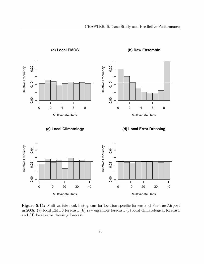
CHAPTER 5. Case Study and Predictive Performance
(a) Local EMOS
Multivariate Rank
Rel
ative
Fre
quen
cy
0 2 4 6 8
0.00
0.10
0.20
(b) Raw Ensemble
Multivariate Rank
Rel
ative
Fre
quen
cy0 2 4 6 8
0.00
0.10
0.20
(c) Local Climatology
Multivariate Rank
Rel
ative
Fre
quen
cy
0 10 20 30 40
0.00
0.02
0.04
(d) Local Error Dressing
Multivariate Rank
Rel
ative
Fre
quen
cy
0 10 20 30 40
0.00
0.02
0.04
Figure 5.11: Multivariate rank histograms for location-specific forecasts at Sea-Tac Airportin 2008: (a) local EMOS forecast, (b) raw ensemble forecast, (c) local climatological forecast,and (d) local error dressing forecast
75

CHAPTER 5. Case Study and Predictive Performance
−5 0 5 10
−50
510
U
V
●
●
●
●
●
●●
●
●●
●
●
●
●
●
●
●
●
●
●
●
●
●
●
●
●
●
●
●
●
●
●
●
●
●
●
●
●
●
●●
●
●
●
●
●
●
●
●
●
●
●
●
●
●
●
●
●
●
●
●
●
●
●
●
●
●
●
●
●●
●
●
●
●
●
●
●
●
●
●
●
●
●
●
●
●
●
●
●
●
●
●
●
●
●
●
●
●
●
●
●
●
●
●
●
●
●
●
●
●
●
●
●
●
●
●
●
●
●
●
●
●
●
●
●
●
●
●
●
●
●
●
●
●
●
●
●
●
●
●
●
●
●
●
●
●
●●
● ●
●
●
●
●
●
●
●
●
●
●
●
●
●
●
●
●
●
●
●
●
●
●
●●
●
●●
●
●
●
●
●
●
●
●
●
●
●
●
●●
●
●
●
●
●
●
●
●
●
●
●
●
●
●
●
●
●
●
●
●
●
●
●
●
●
●
●
●
●
●
●
●
●
●
●
●
●
●
●
●
●
●
●
●
●●
●
●
●
●
●
●
●
●
●
● ●
●
●
●
●
●
●
●
●
●
●
●
●
●
●
●
●
●
●
●
●
●
●
●
●
●
●
●
●
●
●
●
●
Figure 5.12: Marginal calibration diagram for Sea-Tac Airport; each red asterisks representsan observations, each blue dot a random ensemble member and each green diamonds a randomvector from the EMOS predictive distribution
76

CHAPTER 5. Case Study and Predictive Performance
cells, the actual grade of calibration can become distorted. This applies to all climatology anderror dressing histograms in the case study.
Local EMOS is, apart from the uncalibrated raw ensemble, the sharpest forecast, with theclimatological ensemble the least sharp. The Euclidean error shows that the EMOS predictivemedian yields the best point forecast, being slightly better than the error dressing ensemble.Finally, in terms of the energy score, which addresses calibration and sharpness simultaneously,EMOS has the best overall predictive skill, closely followed by the local error dressing approach.The climatological forecast is not competitive, as it is too widely spread and has an evenhigher energy score than the raw ensemble.
In order to check EMOS for marginal calibration, we consider the marginal calibrationdiagram in Figure 5.12. As the verifying observations are discretised, we added a smallrandom noise to each observed vector to simulate the undiscretised distribution and to improveinterpretability. Comparing the empirical distributions, we see that, apart from some outliers,the local EMOS forecast reproduces the observation pattern. Although the UWME has norecognisable biases, it fails to predict the observations in the lower right and upper left and istoo concentrated. So, it can be said that the local EMOS method is marginally calibrated forthis station, while the spread of the ensemble is once more not large enough.
5.4.3 Results for the Pacific Northwest, 1 January - 31 December2008
After examining the performance for one location, we now turn to the results aggregated overall stations in the Pacific Northwest. First we will address the issue of using only the ensemblemean or all ensemble members as predictors for the EMOS mean, as described in 5.2.1.1.Then our new method will successively be compared to the competing forecasts introducedearlier in this chapter.
5.4.3.1 Comparing Simple and Multiple Linear Regression
For the regional EMOS technique, we proposed to employ multiple linear regression based on theensemble member forecasts in order to estimate the predictive mean. To ensure interpretable
77
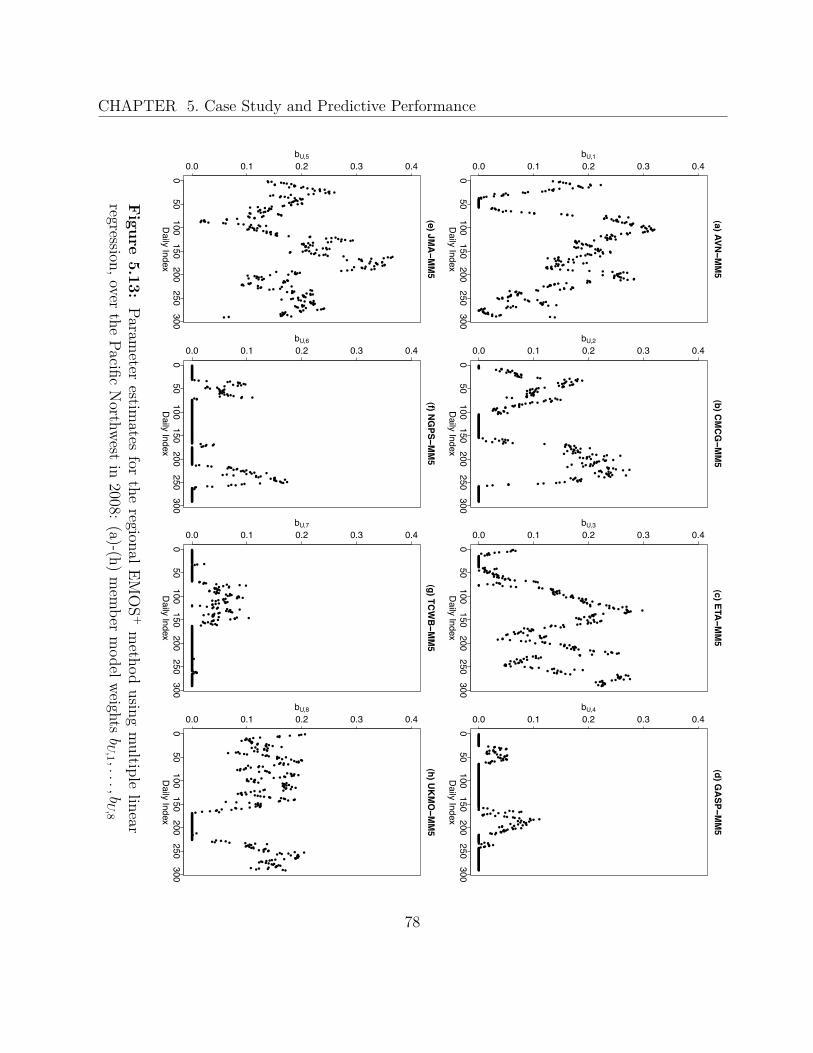
CHAPTER 5. Case Study and Predictive Performance
● ●● ● ● ●● ● ●●● ● ● ●●●●●● ● ●●●●● ●●● ● ●●●●●●●● ●●●●●●●●●●●●●●●●●●●● ● ●● ● ●● ● ●● ● ● ● ● ● ●● ● ● ● ● ●●●● ● ●●● ● ● ●● ● ●●● ●● ● ●● ● ● ●● ● ●● ●● ●●●●●● ●●● ●● ●●● ● ● ● ●●●● ●● ● ●● ● ●● ● ● ●●● ●● ● ●● ●● ● ● ●● ●● ●● ● ●●● ●●●●● ● ● ●● ●● ● ● ● ●●● ● ●●●●●●● ●● ● ● ● ● ● ● ● ● ●●●●●● ● ●● ● ●● ● ●●●●● ● ● ●●●●●●● ●●● ● ● ●● ● ●●● ●● ●● ● ● ●●●● ●●●●●●● ●● ● ●●● ● ●●●● ● ●● ●●●● ●●●●● ●●●● ● ●● ●● ● ● ● ●●● ● ● ●
050
100150
200250
300
0.0 0.1 0.2 0.3 0.4
(a) AVN−M
M5
Daily Index
bU,1
●●●●● ●● ● ●● ● ●● ● ●● ● ● ● ● ●● ●● ● ● ● ● ● ●● ● ●●● ●●● ●● ●●●● ● ●●●●●●● ●●● ● ●●● ●● ● ●● ●●● ●● ● ●● ● ●● ●● ●● ●●●● ●●●● ● ●● ●●●● ●●● ● ●● ● ●●●●●●●●●●●●●●●●●●●●●●●●●●●●●●●●●●●●●●●●●●●●●●●●●●●●●● ● ● ● ● ●●● ●● ● ●● ● ●● ● ●●● ● ● ●●● ● ● ●● ● ● ●●●● ● ● ● ●●●●● ● ● ● ● ●●●●●● ●● ●●● ● ●●●● ● ● ●● ● ●●●● ●● ●● ● ●● ● ●●● ●●●● ● ●● ●● ●●●●●●●●●●●●●●●●●●●●●●●●●●●●●●●●●●●●●●●●●●●●●
050
100150
200250
3000.0 0.1 0.2 0.3 0.4
(b) CM
CG−M
M5
Daily Index
bU,2
●● ●●●●●●● ● ●●●●●●●●●●●●●●●●●●●●●●●●●●●● ●● ●●● ●● ● ●● ●● ●● ●● ● ● ●● ● ● ● ●●● ● ● ● ● ● ●● ● ●● ●●● ● ● ● ●● ● ● ●● ● ●●● ●● ●●● ● ● ●● ●●● ● ● ● ●●●● ● ●●● ● ● ●●● ● ●● ●●●● ● ● ● ● ●● ●●●● ●●●●●● ●●● ●● ●● ● ●● ●●●● ●●●●●●● ●● ●●●● ● ● ● ●● ●●● ● ●●●●● ● ● ●●●● ●●●● ● ●● ● ● ●●● ● ● ● ●●● ●● ●● ●● ●● ● ● ● ● ● ● ●●●●● ●●●● ●● ●●● ●● ●● ● ●●●●●● ●● ● ● ● ● ●● ●● ● ●●● ● ●●● ● ● ● ● ● ●● ●●● ●● ●●●●●●●● ● ● ●●●● ●●
050
100150
200250
300
0.0 0.1 0.2 0.3 0.4
(c) ETA−M
M5
Daily Index
bU,3
●●●●●●●●●●●●●●●●●●●●●●●●●● ● ●● ● ● ●●●●● ●● ●●● ●● ● ● ●●●●● ● ● ● ● ●●●● ●●● ● ●●●●●●●●●●●●●●●●●●●●●●●●●●●●●●●●●●●●●●●●●●●●●●●●●●●●●●●●●●●●●●●●●●●●●●●●●●●●●●●●●●●●●●●●●●●●●●● ● ●●●● ● ● ● ●●●●●●●● ● ● ● ● ● ● ● ● ●●●●● ●●● ●●● ● ●●●●●● ● ●●●●● ●● ●● ●●● ● ●●●●●●●●●●●●●●●●●● ● ●● ● ● ●●●●●●●●●●●●●●●●●●●●●●●●●●●●●●●●●●●●●●●●●●●●●●●●●●●●●●●
050
100150
200250
300
0.0 0.1 0.2 0.3 0.4
(d) GA
SP−MM
5
Daily Index
bU,4
● ●● ● ● ● ●●● ● ●● ●● ● ● ● ● ●●● ● ●● ●● ●●●●●● ● ●● ● ● ● ●●●● ●●●●● ● ●●● ●●●●●● ● ● ●●●● ●● ●●●● ● ● ● ● ●●● ●● ●●●● ●●● ● ●● ● ● ● ● ● ● ● ●●● ● ● ●●●● ● ● ● ● ●●● ●●● ●● ● ● ●● ●●● ● ● ● ●●●●●●●●● ● ● ●●●● ● ●● ●●●●● ●●●● ●● ● ●●● ● ● ●● ●●●● ●● ● ● ● ●●●● ● ● ●●●●●● ● ● ● ●●●●●●● ● ●●● ●●●● ● ● ●●●● ●● ● ● ●● ● ●●●● ●●● ● ● ●●●●● ●●● ● ●● ●● ●● ● ● ●●● ●● ● ●●●●●● ● ● ●● ●● ●● ●● ●● ●● ●● ● ● ●●●●●● ● ●●● ● ●● ● ●●● ●●●
050
100150
200250
300
0.0 0.1 0.2 0.3 0.4
(e) JMA−M
M5
Daily Index
bU,5
●●●●●●●●●●●●●●●●●●●●●●●●●●●●●●● ● ● ● ●● ● ●● ● ●● ●●●● ● ●● ● ● ●● ●●● ● ●● ●● ●● ●● ●● ● ●●● ● ●●●●●●●●●●●●●●●●●●●●●●●●●●●●●●●●●●●●●●●●●●●●●●●●●●●●●●●●●●●●●●●●●●●●●●●●●●●●●●●●●●●●●●●●●●●●●●● ● ●● ●●●●●●●●●●●●●●●●●●●●●●●●●●●●●●●●●●●●●●●●●● ●● ● ● ● ● ●● ●●● ●●● ● ● ● ●●●●● ● ● ●● ● ●●● ● ●● ● ● ● ●● ●●●●● ●●● ●●●●● ●●●●●●●●●●●●●●●●●●●●●●●●●●●●
050
100150
200250
300
0.0 0.1 0.2 0.3 0.4
(f) NG
PS−MM
5
Daily Index
bU,6
●●●●●●●●●●●●●●●●●●●●●●●●●●●●●● ●●●●●●●●●●●●●●●●●●●●●●●●●●●●●●●●●●●●●● ●● ● ●● ● ● ● ●● ●● ●● ●● ●● ●●● ●● ● ●● ●● ●●● ●● ● ●●●●●●● ● ● ●●●●●●●● ●● ● ● ●● ● ● ●●●● ● ● ●●●●● ●● ●● ● ● ● ●● ●●●●●●● ●● ● ● ●● ●●●●●●●●●●●●●●●●●●●●●●●●●●●●●●●●●●●●●●●●●●●●●●●●●●●●●●●●●●●●●●●●●●●●●●●● ●●●●●●●●●●●●●●●●●●●●●●●●●●● ● ● ● ●●●●●●●●●●●●●●●●●●●●●●●●●●●●●
050
100150
200250
300
0.0 0.1 0.2 0.3 0.4
(g) TCW
B−M
M5
Daily Index
bU,7
●●●●●● ●●●● ●●● ●● ● ● ●●● ● ●● ●● ●● ●●● ●●● ● ● ●● ●●●● ● ● ● ● ●● ● ● ●●●● ● ● ● ●● ●● ●● ●● ●●●● ● ●●●●●● ●● ● ● ●● ● ● ● ● ●● ●●●● ●●●●●● ●●● ● ● ● ● ●● ● ● ●●● ● ●● ●●● ●●● ●● ●●●●●● ●● ● ● ● ● ● ● ● ● ● ●●●●●● ● ● ● ●● ● ●● ●● ●●● ● ●● ●●●●● ●●●●●●●●●●●●●●●●●●●●●●●●●●●●●●●●●●●●●●●●●●●●● ●●● ●●●●●●●●●●●● ● ● ●● ● ● ● ● ●● ●●●● ● ●● ● ●●●● ●●● ● ●● ●●● ●● ● ●● ●●● ●●●●●●● ●● ● ● ●● ● ● ●●●●●● ● ●● ● ●
050
100150
200250
300
0.0 0.1 0.2 0.3 0.4
(h) UK
MO−M
M5
Daily Index
bU,8
Figure
5.13:Param
eterestim
atesfor
theregionalEM
OS
+m
ethodusing
multiple
linearregression,over
thePacific
Northwest
in2008:
(a)-(h)m
ember
modelweights
bU
,1 ,...,bU
,8
78
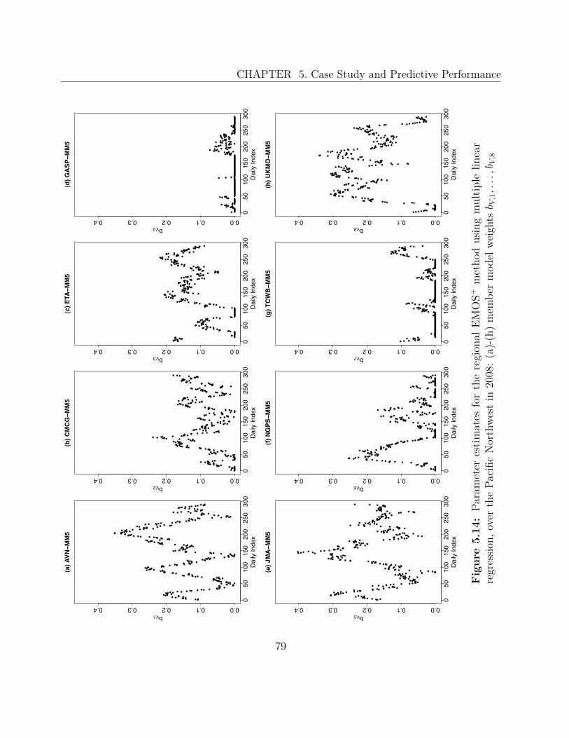
CHAPTER 5. Case Study and Predictive Performance
●● ●●●● ●●● ●● ●●● ●● ● ●●●● ● ●● ●● ● ●● ● ●● ● ● ●● ● ●● ● ●●● ● ● ●●● ●● ●● ●● ●●●● ●●● ●● ●● ●●● ●●● ●●●● ●●● ● ●
●● ●●● ●●
● ●●● ●● ● ● ●
●● ● ● ● ●●● ● ● ●● ● ●●● ● ● ●●●● ●● ●●● ●●● ●● ● ● ● ● ●●● ● ●●● ●●● ●●●● ●●● ● ● ● ● ●● ●● ●● ●● ● ●●● ●●●●●● ●● ●●●● ● ●●●● ● ●● ●●●●●●●●●●● ●● ●● ●●●● ● ● ● ● ●●●● ● ● ● ● ●●●● ● ●●● ● ● ●●●● ● ● ● ● ● ● ● ●● ● ●● ●●●●● ●● ● ● ●● ●● ●●●●● ●● ●●●●● ● ● ●● ● ● ●● ●●●●● ● ● ● ● ● ● ● ● ●● ●
050
100
150
200
250
300
0.00.10.20.30.4
(a) A
VN−M
M5
Dai
ly In
dex
bV,1
● ●● ●●●●
● ● ●●
● ●● ●● ●●●●● ●● ●●●● ●● ● ● ● ● ●●●●●●●●● ●● ●● ● ● ●●● ●● ●● ●● ● ●● ●●●●● ●●●●●●● ●●●● ●●● ● ● ●● ●
● ●● ●● ● ●●● ●●●●●● ●●● ● ● ● ● ● ●● ●● ●● ● ● ● ● ●● ● ●●●● ● ● ● ●● ●● ●●● ●● ● ●● ● ● ● ●●●● ●● ● ● ●●●●●●● ●●● ● ● ● ●●●●●● ● ● ● ●●● ● ● ● ●●●●
●● ●●●● ●●● ●●●● ●● ●●●●● ●● ● ● ● ● ● ●●●● ● ● ●●● ● ● ●
● ● ● ●● ●● ● ● ● ● ●● ●●●●●●●●● ●● ●●● ●●● ● ● ●● ●
●●● ●●● ●●● ● ●●● ● ●●
● ●●● ●● ● ● ●● ●● ●● ●●●●●
050
100
150
200
250
300
0.00.10.20.30.4
(b) C
MC
G−M
M5
Dai
ly In
dex
bV,2
● ●● ● ● ●● ● ●●●● ● ●●●●● ● ●●●●●●●●●●●●● ●●● ●● ●●●● ● ●●●●●●● ● ● ●●●● ●
● ●● ●● ● ● ●● ●● ●● ● ●● ● ●● ●●●●●●●●●●●●●●●●●●●●●●●●●●●●●●● ●● ●● ● ●●●●●● ●●●● ● ● ● ●● ●● ●● ●●● ●● ● ●● ● ●
●●● ● ● ●●● ●● ●● ● ● ●● ●● ● ● ●●● ● ● ●● ●● ●● ● ● ● ●●●●● ● ● ● ●●● ● ●●● ● ● ●●● ● ●● ● ● ● ● ● ●●● ● ● ● ●● ● ● ●●● ●● ● ● ●●●●● ● ●● ●●●●●● ●●● ● ●●
● ● ●● ● ●● ●●●● ●●●● ●● ● ● ●●● ●●●●●● ● ● ● ● ● ●●● ● ●●● ● ●● ●● ● ●●●● ● ●
050
100
150
200
250
300
0.00.10.20.30.4
(c) E
TA−M
M5
Dai
ly In
dex
bV,3
● ●●●●●●●●●●●●●●●● ● ●●●● ●● ● ●●● ●●●●
●●●●●●●●●●●●●●● ● ● ●●●●
●●●●●●●●●●●●●●●●●●●●●●●●●●●●●●●●●●●●●●●●●●●●●●●●●●●● ● ● ● ●●●
●●●●●●●●●●●●●●●●●●●●●●●●●●●●●●●●●●●●●●●●●●●●●●●●●●●●●●●●●●●●●●●● ●● ● ● ●● ●● ● ●●● ● ●● ● ●● ● ● ●● ●●●● ● ● ● ● ● ● ● ●●●●●● ●●● ● ●●● ●
● ●● ● ●●● ●●● ●● ●●● ●
● ●●● ●●●●●● ●●●●●●●●●●● ●●●● ● ●●●●●●●●●●●●●●●●●●●●●●●●●●●
050
100
150
200
250
300
0.00.10.20.30.4
(d) G
ASP−M
M5
Dai
ly In
dex
bV,4
●● ●●●●● ● ●● ● ●●● ● ● ● ●● ● ●●● ●● ● ● ●●● ● ●● ● ● ● ●● ●● ●●● ● ● ● ● ● ● ● ● ●● ●● ●●●● ● ● ●●
● ●● ● ●● ●●● ●● ●●● ● ●● ● ● ● ●● ●●●●●●● ●●●● ● ● ●●● ● ●●● ●●●● ●●● ● ●● ●●●●●●● ●●●● ● ● ●●● ●● ● ●●●●● ●●●● ● ●●● ● ● ● ● ●●● ● ● ● ● ●● ●●●● ● ●●●● ●●● ●●● ● ●●● ●● ● ● ● ● ● ● ●●● ● ● ● ●●●●●● ● ● ●●●● ● ●●● ● ● ● ●● ● ● ● ●●●●●
●●●●● ● ● ● ●●●●● ● ● ●● ● ● ●
● ● ●● ● ● ● ●●●● ●● ●● ●●● ● ● ● ● ● ● ●●●●●● ●● ● ●● ● ● ●●●● ● ●●●●●●●
050
100
150
200
250
300
0.00.10.20.30.4
(e) J
MA−M
M5
Dai
ly In
dex
bV,5
●●●●●●● ●●●●●●●● ●●● ● ● ●● ●●●●● ●●●●●● ●● ●●● ● ● ● ● ●● ● ●●●● ●●● ●● ● ●●●●● ●● ● ● ●● ●●● ● ● ●●● ●● ●● ● ● ● ●● ● ●
● ● ● ●● ● ● ● ● ● ● ●●● ● ● ●●● ●
●●●●●●●●●●●●●●●● ● ●●●
●●●●●● ●●● ●● ● ● ●●●● ●●●●●●● ● ● ●● ●●●●●● ● ●● ●● ●● ● ● ● ● ● ● ● ●● ●●●●● ●●●●● ● ● ●● ●●● ● ● ● ● ●●●
●● ●● ●● ●●●●● ● ● ● ●●● ● ● ●●●● ●●● ●●●●●●●●●●●●● ●●●●●●●●●●●
●● ●●● ●●● ● ●●●●●●●●●● ● ●● ●● ●●●●
●●●●●●●●● ●●● ● ●
050
100
150
200
250
300
0.00.10.20.30.4(f)
NG
PS−M
M5
Dai
ly In
dex
bV,6
● ● ● ● ● ● ●● ●● ● ●● ●●●●●●●●●●● ●● ●●●●●●●●●●●●●●●●●●●●●●●●●●●●●●●●●●●●●●●●●●●●●●●●●●●●●● ● ●●●●●●●● ●●● ● ●● ● ●● ●●● ●● ● ●● ● ●●● ●●●●● ●● ● ● ●●●●
●●●● ●●●●●●●●●●●●●●●●●●●●●●●●●●●●●●●●●●●●●●●●●●●●●●●●●●●●●●●●●●●●● ●●
●● ●● ● ● ● ● ● ● ●● ●●●●●●● ● ● ●●●●
●● ● ● ●● ● ● ●●● ●●●●●●●●●●●●●●●●●●●●●●● ●●●● ●● ●●●●● ●●●●● ●● ●●● ●●● ● ●● ● ● ●●●
●●●●●● ● ●● ●
050
100
150
200
250
300
0.00.10.20.30.4
(g) T
CW
B−M
M5
Dai
ly In
dex
bV,7
● ● ● ● ● ●● ● ●●●● ●●●●●●●●●●●● ●● ●
● ●●●●●●●● ● ● ● ●●●●●●● ●●●●●● ● ●
●● ● ● ●●● ● ●●●● ● ●● ● ●● ● ●●●● ● ● ●●● ●● ●● ● ● ● ● ● ●●● ● ● ● ●● ●●●●● ●●●● ●● ●●● ●● ●●● ● ● ● ●● ●● ●●●● ●● ● ●
●● ●●● ●● ● ● ● ● ● ● ● ●●●● ●●● ● ●● ●●●●●●●●● ● ● ●●●●● ● ●● ● ●●●●●●●● ● ●● ● ● ●● ● ● ●● ● ● ● ● ●● ● ● ●●●●● ● ● ● ●●● ● ●● ● ●●●● ●●● ● ● ● ●● ● ●●●●● ● ● ● ● ●●●● ● ●● ● ● ●●●● ●●● ● ●●● ●
● ● ● ● ● ●● ● ● ● ● ● ● ● ●●●●● ●●● ●●●● ●● ●
050
100
150
200
250
300
0.00.10.20.30.4
(h) U
KM
O−M
M5
Dai
ly In
dex
bV,8
Fig
ure
5.14
:Pa
ram
eter
estim
ates
for
the
regi
onal
EMO
S+m
etho
dus
ing
mul
tiple
linea
rre
gres
sion,
over
the
Paci
ficN
orth
west
in20
08:
(a)-
(h)
mem
ber
mod
elwe
ight
sb V
,1,.
..,b
V,8
79

CHAPTER 5. Case Study and Predictive Performance
member weights bU,1, . . . , bU,8 and bV,1, . . . , bV,8, we employ a variant of EMOS+, and eliminatepredictors from the regression equation until there are only non-negative coefficients left.
When we take a look at these coefficients in Figures 5.13 and 5.14, the predictive skill of theindividual member models can directly be compared. For both components, the AVN-MM5and JMA-MM5 forecasts received the highest weights, which corresponds well with the resultsin Thorarinsdottir and Gneiting (2010), obtained over the same test period. The forecastsgenerated using the initial conditions by the Australian Bureau of Meteorology, GASP, and bythe Taiwan Central Weather Bureau, TCWB, had the lowest weights throughout the year,being zero most of the time. Interestingly, the NGPS-MM5 member shows almost no skillfor the U component, but gets rather solid weights for V . Although the AVN-MM5 and theETA-MM5 forecasts are obtained with initial data from the same source, the National Centersfor Environmental Prediction, their coefficient estimates are both substantial over the wholetest period, which indicates that they are not highly correlated.
In Figures 5.15 and 5.16, we see the estimated parameters for the intercept and thepredictive variances. We notice that, in comparison to the local parameters in Figure 5.10,dU and dV never vanish. This increased stability is due to the higher amount of trainingdata available for the regional technique. The ensemble for the V component shows a muchmore prominent spread-error correlation than the one for the U component, as the valuesfor cV are very small, while dV tends to be large. Again, the coefficients cU and dU exhibitan anti-cyclical behaviour, suggesting a varying relationship between ensemble spread andforecast skill.
Considering the scores in Table 5.6, for both simple and multiple regression techniques, andthe multivariate rank histograms in Figure 5.17, we notice a small improvement in performancewhen using all ensemble members to predict the EMOS mean. Not only implies the lowerEuclidean error a more accurate deterministic forecast, but the EMOS+ version is also bettercalibrated and sharper, leading to a lower energy score. The results show that the assumptionof exchangeable ensemble members does not apply to the UWME, although it apparently causesonly a minor loss in predictive skill to use the ensemble mean as sole predictor. Therefore, itseems worthwhile to keep simple linear regression for the local approach, where we have lesstraining data, and adopt multiple linear regression for the regional technique.
80

CHAPTER 5. Case Study and Predictive Performance
●
●●
●●
●●●
●●●●
●
●●●
●●●●●●●●●●●●●●
●●●●●●●●●●
●
●
●
●
●●●
●
●
●●●
●●●●●●●
●
●●●●●●●
●
●●●●●●
●●●
●●●●●●●●●●●
●
●●●●●
●●
●●●●
●●●
●
●●●●●●●●
●
●
●
●●
●●●
●
●●●
●●●
●
●●
●●●●
●●●●●●●●
●●
●●●●●●●●●
●●●●●●●●
●●●
●●●
●
●
●
●●●●●●●●●●
●●●
●
●●●●
●
●●●●
●●●
●
●●●●●●
●●
●
●●●●●●●●●●●
●●●●●●●●●●●
●
●●●●
●●●●●●●●●●
●
●●●●●●●●●
●●●●●●●●●●●●●●●●●●●●
●●●●●
●●●●●●
●
●
●
●●●●
0 50 100 200 300
−0.6
−0.4
−0.2
0.0
0.2
0.4
(a)
Daily Index
a U
●
●●●●●
●●●●●●●●●●●●●●●●●
●●●
●●●●●●●
●●
●
●
●
●●●●●●●●●●●●●●●●●●●
●●●●●●●●
●●●
●●●●●●
●●●●●●●●●●●●●●●●●●●●
●●
●
●●
●●
●●●●●●●●●●●●●
●
●●●
●
●●
●●●●●
●●●●●●●●●●
●●●●●●●●●●●●●●●●●●●●
●
●●●●●
●●●●●●●●●●●●●●●●●●●●●●●●●●●●●●●●●●●●●●●●●●●●●●
●●●●●●
●●●●
●●●●●●●●●●●●●
●●
●
●●●●●●●●●●●●●●●●●●●●●●●●●●●
●●●
●●●●●
●●●●
●●●●
●●●●●●●●●
●●●●●
0 50 100 200 300
01
23
45
(b)
Daily Index
c U
●●●●●●
●●●●●●●●●●●●●●●●●●●●●●●●●●●●●●
●
●●●●●●●●●●●●●●●
●●●●●
●●●●●●●●●●●●●●●●●●●●●●●●●●●●●●
●●●●●●●●●●●●●●●●●●●●●●●●●●●●●●●●●
●●●●●●●●●●●●●●●●●●●●●●●●
●●●●●●●
●●●●
●●●●●●●
●●●●●●●
●●●●●
●●
●●●●●●●
●●●●●●●●●●●
●●●●●●●●●●●●●●●●●●●●●●●●●●●●●●●●
●
●●●●●●●●●●●●●●●●●●●●●●●●●●●●●●
●●●●
●●
●●●●●●●●●●●●
●●
●●●●●●●●●●●●
●●
0 50 100 200 300
01
23
45
(c)
Daily Index
d U
Figure 5.15: Parameter estimates for the regional EMOS+ method using multiple linearregression, over the Pacific Northwest in 2008: (a) intercept aU , (b) and (c) variance coefficientscU and dU
5.4.3.2 Results for Regional Forecasts
In this section, we assess the performance of the regional EMOS+ method as compared toother regional forecasting techniques and the unprocessed UWME ensemble. We concentrateon the multiple regression version and give results in terms of the energy score, Euclideanerror, multivariate rank histogram and determinant sharpness.
Looking at the histograms in Figures 5.17 and 5.18, we find that the bivariate EMOS+,climatological and error dressing forecasts, as well as the ECC ensemble, generated using theregional EMOSUV distributions, are nearly calibrated, while the regional EMOSUV method itselfis overdispersive. The latter is however not surprising, as this technique predicts independentvector components and the respective variances are estimated individually. Therefore, inorder to capture outlying observations, the spread is enlarged in both dimensions, and bythat overestimated. The multivariate histogram for the UWME in Figure 5.20 shows the rawensemble’s underdispersion clearly, as seen before when we considered only one station.
81
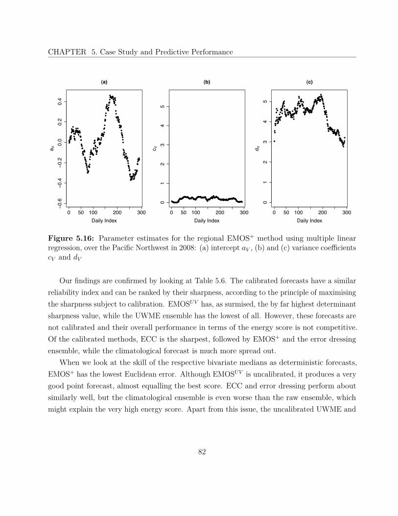
CHAPTER 5. Case Study and Predictive Performance
●●●●●●●
●●●
●
●●●●●
●
●●●
●
●●●●
●●●●
●●●●●●●●
●●
●●●●●●●
●●●
●●
●●●●●
●●
●●●●●●●
●●●●
●●●●●●●
●●●●●
●●●●
●
●●
●●●●●●●●●●●●●
●●
●●●●●
●
●●
●●
●●●●
●
●●●●●●●
●●●●●●
●●●
●●●●●●●●●●
●
●
●
●
●●●
●●
●●●●●
●●●●●
●●●●●
●
●●●●●●●●●●
●●●●●●●●●●
●●●
●
●
●
●●●●●
●●●●
●●●
●
●●●●●●●●
●●●●●●●
●
●
●●●●●●●●●●●
●●●●●●
●●●●●●●●●
●●●
●●●●●
●●●●●●●●
●●●●●●
●
●●●●●●●●
●●
●●●●●●●
0 50 100 200 300
−0.6
−0.4
−0.2
0.0
0.2
0.4
(a)
Daily Index
a V
●●●●●●●●●●●●●●●●●●●●●●●●●●●●●●●●●●●●●●●●●●●●
●●●●●●●●●●●●●●●●●●●●●●●●●●●●●●●●●●●●●●●
●●●●●●●●●●●●●●●●●●●●●●●●●●●●●●●●●●●●●●●●●●●●●●●●●●●●●●●●●●●●●●●●●●●
●●●●●●●●●●●●●●●●●●●●●●●●●●●●●●●●●
●●●●●●●●●●●●●●●●●●●●●●●●●●●●●●●●●●●●●●●●●●●●●●●●●●●●
●●●●●●●●●●●●●●●●●●●●●●●●●●●●●●●●
●●●●●●●●●●●●●●●●●●●●●●●●
0 50 100 200 300
01
23
45
(b)
Daily Index
c V
●
●●
●●●
●●
●
●
●●
●
●
●●●●●●●
●
●●
●
●
●
●
●●●●
●
●●
●●●●●●
●
●●●●●●●●
●●●●
●●
●●●●●●●●●●●●●●●●●●●
●
●●●●●
●●
●
●
●
●●
●●●●●●●●
●●●●●
●●
●●●●●
●●●●●●
●●●●●
●
●
●●
●
●●●
●●●●
●●●●●●●●●●●●●●●
●●●●●●●●●●●●●●●●●●●●●●●●●●●●●●●●●●●●●●●●
●●●●●●●●●●●●●●●●●●●●●
●●●●●●●●●●●
●
●●●
●●●
●●●●●●●●●●●●●●●●●●●●●●●●
●●●●●●●●●●●●●●●●●●
●●●●●●●●●●●●●●●●●●●
●●●●
●
0 50 100 200 300
01
23
45
(c)
Daily Index
d V
Figure 5.16: Parameter estimates for the regional EMOS+ method using multiple linearregression, over the Pacific Northwest in 2008: (a) intercept aV , (b) and (c) variance coefficientscV and dV
Our findings are confirmed by looking at Table 5.6. The calibrated forecasts have a similarreliability index and can be ranked by their sharpness, according to the principle of maximisingthe sharpness subject to calibration. EMOSUV has, as surmised, the by far highest determinantsharpness value, while the UWME ensemble has the lowest of all. However, these forecasts arenot calibrated and their overall performance in terms of the energy score is not competitive.Of the calibrated methods, ECC is the sharpest, followed by EMOS+ and the error dressingensemble, while the climatological forecast is much more spread out.
When we look at the skill of the respective bivariate medians as deterministic forecasts,EMOS+ has the lowest Euclidean error. Although EMOSUV is uncalibrated, it produces a verygood point forecast, almost equalling the best score. ECC and error dressing perform aboutsimilarly well, but the climatological ensemble is even worse than the raw ensemble, whichmight explain the very high energy score. Apart from this issue, the uncalibrated UWME and
82

CHAPTER 5. Case Study and Predictive Performance
(a) Regional EMOS+
Multivariate Rank
Rel
ative
Fre
quen
cy
0 2 4 6 8
0.00
0.10
0.20
Multiple Regression(b) Regional EMOS
Multivariate Rank
Rel
ative
Fre
quen
cy0 2 4 6 8
0.00
0.10
0.20
Simple Regression
(c) Regional Climatology
Multivariate Rank
Rel
ative
Fre
quen
cy
0 10 20 30 40
0.00
0.02
0.04
(d) Regional Error Dressing
Multivariate Rank
Rel
ative
Fre
quen
cy
0 10 20 30 40
0.00
0.02
0.04
Figure 5.17: Multivariate rank histograms for regional forecasts over the Pacific Northwestin 2008: (a) regional EMOS+ forecast using multiple linear regression, (b) regional EMOSforecast using simple linear regression, (c) regional climatological forecast, and (d) regionalerror dressing forecast
83

CHAPTER 5. Case Study and Predictive Performance
(a) ECC
Multivariate Rank
Rel
ative
Fre
quen
cy
0 2 4 6 8
0.00
0.05
0.10
0.15
0.20
(b) Regional EMOSUV
Multivariate Rank
Rel
ative
Fre
quen
cy0 2 4 6 8
0.00
0.05
0.10
0.15
0.20
(c) Local EMOSUV
Multivariate Rank
Rel
ative
Fre
quen
cy
0 2 4 6 8
0.00
0.05
0.10
0.15
0.20
Figure 5.18: Multivariate rank histograms for competing forecasts over the Pacific Northwestin 2008: (a) ECC ensemble forecast based on regional EMOSUV , (b) regional EMOSUV forecast,and (c) local EMOSUV forecast
84

CHAPTER 5. Case Study and Predictive Performance
Table 5.6: Comparison of the regional forecasting techniques and the raw ensemble in termsof proper scoring rules, calibration and sharpness, averaged over the Pacific Northwest in 2008
Method ES EE ∆ DS
Regional EMOS+ 2.005 2.792 0.020 2.254Regional EMOS 2.011 2.802 0.026 2.272Regional climatology 2.677 3.632 0.019 2.924Regional error dressing 2.181 3.002 0.023 2.380ECC ensemble 2.325 2.998 0.024 1.859Regional EMOSUV 2.432 2.798 0.365 4.701Raw ensemble 2.467 3.006 0.528 0.819
EMOSUV expectedly receive the largest energy score values. The bivariate EMOS+ methodclearly performs better than the other techniques.
Surprisingly, the ECC ensemble has a relatively high energy score, though being calibratedand the sharpest forecast of all. In Section 2.2, we mentioned that the determinant sharpnesstends to overly reward strongly calibrated forecasts, although the variances might be large.Figure 5.19 pictures the predictive correlation of the regional EMOS+ method and the empiricalcorrelation for the ECC ensemble at one station. This graphical comparison shows that ECCpredicts correlations ranging from −1 to 1, while the EMOS+ correlation always lies between−0.4 and 0.1. We can conclude that these high correlations estimates distort the actual spreadof the ECC approach and the true performance relative to EMOS+ reveals itself in the energyscore. Possibly, this effect is caused by the relatively small ensemble size of eight; in order tocompute the determinant sharpness, we fit a normal distribution to the ensembles using theempirical variances and correlation. However, when applied to a large ensemble, the empiricalcorrelation can be estimated more accurately.
Summing up, we notice that the two-dimensional EMOS+ method clearly outperformsthe other regional forecasting and postprocessing techniques. EMOSUV overestimates thebivariate spread, and when additionally combined with the ECC approach, overestimates thecorrelation. Our way of predicting the correlation depending on the predicted wind direction
85

CHAPTER 5. Case Study and Predictive Performance
0 50 100 150 200 250
−1.0
−0.5
0.0
0.5
1.0
Daily Index
Cor
rela
tion
●
●
●●
●
●
●
●
●
●
●●●●
●●
●●
●
●
●
●
●
●
●●
●
●
●
●●
●●●●
●
●●●
●●
●●●
●
●
●
●
●
●
●●
●
●●
●
●
●●
●●●●
●●
●
●●●●●●
●
●●●●●●●
●
●●●●●
●●
●
●
●
●●
●
●
●
●
●
●
●
●
●
●●●●
●
●
●
●●
●●
●
●●●
●
●
●
●●●
●
●
●●
●
●
●
●●●
●●
●
●
●
●●●
●
●
●●●
●
●●●●●
●
●
●
●
●●
●
●●
●
●
●
●
●
●
●●●●
●
●●●
●
●●
●
●
●●●●●
●
●●●●●●●●●●
●●
●
●
●●
●●
●
●
●●
●
●
●
●
●
●
●●
●
●●
●●
●
●
●
●
●
●●
●
●
●
●
●
●●
●
●
●
●
●●●●●●●
●
●
●
●
●●
●
●
●●●
●●
●
●●●
●●●●
●
●
●
●
●●
●●
●●●
●
●
●
Figure 5.19: Predicted correlation at Sea-Tac Airport in 2008, the green dots represent theregional EMOS+ and the magenta asterisks the ECC method
seems to be essential for the good performance of EMOS+. Though the climatological forecastis calibrated, its median is a poor deterministic forecast and on average, the prediction ellipsesare too wide. The error dressing method produces good results, but is still not as sharp asEMOS+ and therefore has a higher energy score.
5.4.3.3 Results for Local Forecasts
After having seen results for the predictive skill of the local EMOS technique at Sea-TacAirport, we now want to assess the performance for all 79 stations in the Pacific Northwest.In Figures 5.18 and 5.20, the multivariate histograms for the different local approaches areprovided. Although the local EMOSUV technique seems a little more calibrated than theregional version, it is still overdispersive, due to the lack of correlation between the vector
86

CHAPTER 5. Case Study and Predictive Performance
(a) Local EMOS
Multivariate Rank
Rel
ative
Fre
quen
cy
0 2 4 6 8
0.00
0.10
0.20
0.30
(b) UWME Ensemble
Multivariate Rank
Rel
ative
Fre
quen
cy0 2 4 6 8
0.00
0.10
0.20
0.30
(c) Local Climatology
Multivariate Rank
Rel
ative
Fre
quen
cy
0 10 20 30 40
0.00
0.02
0.04
0.06
(d) Local Error Dressing
Multivariate Rank
Rel
ative
Fre
quen
cy
0 10 20 30 40
0.00
0.02
0.04
0.06
Figure 5.20: Multivariate rank histograms for different forecasts over the Pacific Northwestin 2008: (a) local EMOS forecast, (b) UWME forecast, (c) local climatological forecast, and(d) local error dressing forecast
87

CHAPTER 5. Case Study and Predictive Performance
Table 5.7: Comparison of the local forecasting techniques and the UWME in terms of properscoring rules, calibration and sharpness, averaged over the Pacific Northwest in 2008
Method ES EE ∆ DS
Local EMOS 1.875 2.608 0.025 1.906Local climatology 2.404 3.361 0.023 2.421Local error dressing 2.064 2.863 0.025 2.185Local EMOSUV 2.279 2.612 0.213 3.716Raw ensemble 2.467 3.006 0.528 0.819
components. Again, EMOS, the climatological ensemble and the error dressing ensembleare calibrated, as can also be seen by means of the reliability index given in Table 5.7. Wehave established before that the UWME forecast is underdispersive, i.e uncalibrated, andeven though its determinant sharpness is minimal, this results in a high energy score. Beingoverdispersed, EMOSUV also is the least sharp forecast and not competitive in terms of theenergy score, although its median has a very high deterministic forecast skill.
Only considering the calibrated methods, EMOS is sharper than error dressing and bothare sharper than the climatological forecast. Therefore, EMOS also has by far the lowestenergy score, followed by error dressing and climatology. As could be expected, all localmethods perform better than the regional ones, especially in terms of sharpness. Looking at theEuclidean error, we find that the climatological forecast again seems to have no deterministicforecast skill, being even worse than the raw ensemble. The error dressing ensemble is somewhatworse than EMOS, which again produces the best point forecasts.
As with the regional method, we can conclude that EMOS performs better than all otherforecasting and postprocessing methods, in terms of the energy score, the Euclidean error andthe determinant sharpness. The localised approach resulted in an energy score improvementof 6.5% and an increase in sharpness of 15%. Though the climatological and error dressingensembles are calibrated, they are not as sharp as EMOS and therefore have higher energyscores. EMOSUV is again overdispersed and has too wide prediction ellipses, but shows somepredictive skill as deterministic forecast.
88
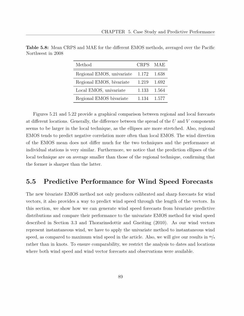
CHAPTER 5. Case Study and Predictive Performance
Table 5.8: Mean CRPS and MAE for the different EMOS methods, averaged over the PacificNorthwest in 2008
Method CRPS MAE
Regional EMOS, univariate 1.172 1.638Regional EMOS, bivariate 1.219 1.692Local EMOS, univariate 1.133 1.564Regional EMOS bivariate 1.134 1.577
Figures 5.21 and 5.22 provide a graphical comparison between regional and local forecastsat different locations. Generally, the difference between the spread of the U and V componentsseems to be larger in the local technique, as the ellipses are more stretched. Also, regionalEMOS tends to predict negative correlation more often than local EMOS. The wind directionof the EMOS mean does not differ much for the two techniques and the performance atindividual stations is very similar. Furthermore, we notice that the prediction ellipses of thelocal technique are on average smaller than those of the regional technique, confirming thatthe former is sharper than the latter.
5.5 Predictive Performance for Wind Speed ForecastsThe new bivariate EMOS method not only produces calibrated and sharp forecasts for windvectors, it also provides a way to predict wind speed through the length of the vectors. Inthis section, we show how we can generate wind speed forecasts from bivariate predictivedistributions and compare their performance to the univariate EMOS method for wind speeddescribed in Section 3.3 and Thorarinsdottir and Gneiting (2010). As our wind vectorsrepresent instantaneous wind, we have to apply the univariate method to instantaneous windspeed, as compared to maximum wind speed in the article. Also, we will give our results in m/s
rather than in knots. To ensure comparability, we restrict the analysis to dates and locationswhere both wind speed and wind vector forecasts and observations were available.
89

CHAPTER 5. Case Study and Predictive Performance
●
●
●
●
●
●
●
●
−124 −122 −120 −118 −116
4243
4445
4647
4849
3 m/s
Figure 5.21: Map of the US states of Washington, Oregon and Idaho, showing the UWMEmeans in blue, the regional EMOS means and 80% prediction ellipses in green, and theverifying observations in red, for a selection of 30 observational locations, valid on 23 January2008
90

CHAPTER 5. Case Study and Predictive Performance
●
●
●
●
●
●
●
●
−124 −122 −120 −118 −116
4243
4445
4647
4849
3 m/s
Figure 5.22: Map of the US states of Washington, Oregon and Idaho, showing the UWMEmeans in blue, the local EMOS means and 80% prediction ellipses in green, and the verifyingobservations in red, for a selection of 30 observational locations, valid on 23 January 2008
91
CHAPTER 5. Case Study and Predictive Performance
First, we compute the univariate EMOS predictive distributions for the regional and thelocal techniques, following the suggestion of 20 and 40 days training period length, respectively.Then, in order to convert wind vectors into wind speed, we sample from the bivariate predictivedistributions 100 times and apply the Euclidean norm to each vector, obtaining the vectorlength and therefore an ensemble of wind speed forecasts.
For assessing the predictive skill, the mean CRPS, mean MAE, PIT histogram andverification rank histogram are employed, in the way they are described in Chapter 2. InFigure 5.23, we see the four histograms for the individual techniques. At first sight, theydon’t seem to be calibrated and rather show a large spike at zero, which means that bothapproaches fail to predict very low wind speed. Probably this is caused by the discretisationof the wind speed observations (Section 5.1), especially as values smaller than 1 knot arerecorded as 0. For maximum wind speed, this was only the case for 30 observations, whereasfor instantaneous wind speed there are more than 2,700 observations equal to 0, i.e. in 14% ofall forecast cases.
However, this problem only arises in the PIT and rank histograms. When we look at theresults of the proper scoring rules, we see that, in terms of the CRPS, both univariate andbivariate methods perform equally well for the local technique, while the univariate EMOSmedian is a better deterministic forecast than the median of the ensemble created from thebivariate EMOS distribution. The difference is quite large for the regional techniques, wherethe univariate method outperforms the bivariate, in terms of both the CRPS and the MAE.
We can summarise that the two EMOS methods seem to have a certain bias, althoughthis impression is probably due to discretisation of the observational data. The univariatetechnique has the higher predictive skill for probabilistic and point forecasts, although theyperform equally well in the localised case. This is only natural, as it was specifically designedand optimised for wind speed, while the bivariate approach issues wind speed forecasts onlyas a byproduct.
Concluding this chapter, we note that the new bivariate EMOS method is a very efficientand successful way to postprocess ensemble forecasts for wind vectors. It corrects the un-derdispersion of the raw ensemble in order to produce calibrated bivariate distributions. An
92

CHAPTER 5. Case Study and Predictive Performance
(a) Regional EMOS
PIT Value
Den
sity
0.0 0.2 0.4 0.6 0.8 1.0
0.0
1.0
2.0
3.0
Wind Speed(b) Regional EMOS
Verification Rank
Rel
ative
Fre
quen
cy0 20 40 60 80 100
0.00
00.
010
0.02
00.
030
Wind Vectors
(c) Local EMOS
PIT Value
Den
sity
0.0 0.2 0.4 0.6 0.8 1.0
0.0
1.0
2.0
3.0
Wind Speed(d) Local EMOS
Verification Rank
Rel
ative
Fre
quen
cy
0 20 40 60 80 100
0.00
00.
010
0.02
00.
030
Wind Vectors
Figure 5.23: Calibration assessment for wind speed forecasts over the Pacific Northwestin 2008: (a) PIT histogram for the univariate regional EMOS method, (b) verification rankhistogram for the bivariate regional EMOS+ method, (c) PIT histogram for the univariatelocal EMOS method, and (d) verification rank histogram for the bivariate local EMOS method
93

CHAPTER 5. Case Study and Predictive Performance
important feature is the estimation of the correlation factor using the predicted wind direction,which results in a low determinant sharpness. In terms of proper scoring rules, EMOS receivedboth the lowest energy score and Euclidean error. Although it might be slightly uncalibrated,the wind speed forecasts created by applying the Euclidean norm are almost as skillful as forthe specialist univariate EMOS method.
94

Chapter 6
Summary and Discussion
In the introduction, we established that there is a huge need for probabilistic forecasts inthe form of calibrated and sharp full predictive distributions. They can be obtained bystatistical postprocessing of ensemble forecasts, which are generated by numerical weatherprediction models and represent possible future states of the atmosphere. Most ensemblesare underdispersive and don’t account for all uncertainties involved in numerical weatherprediction. Postprocessing techniques like EMOS or BMA yield very good results, as theyimprove the predictive performance of the unprocessed ensemble substantially.
So far, these methods were applied to univariate weather variables like temperature, airpressure or precipitation. When considering surface wind, one has only the possibility toaddress one-dimensional features like wind speed, wind direction or one of the zonal andmeridional wind components. However, by employing univariate postprocessing, essentialcharacteristics may not be captured. Therefore we proposed a bivariate variant of EMOS, whichapplies to the wind components jointly rather than separately and thus creates two-dimensionalwind vector forecasts.
Empirical analysis of wind component data yielded that the observations, conditionalon the ensemble forecasts, can be modelled with a bivariate normal distribution, therebyallowing for a similar approach as with univariate EMOS. A straightforward way to expressthe predictive mean vector in terms of the ensemble is to write the individual means as linearregression equations, with the ensemble mean or the ensemble member forecasts as predictors.The parameters are estimated on a sliding training period, typically of 30 or 40 days. In
95
CHAPTER 6. Summary and Discussion
order to make use of a possible spread-skill relationship, we employ an affine function of theensemble spreads for the predictive variances. Here, maximum likelihood estimation ensuresthat calibration and sharpness of the predictive distribution are addressed simultaneously.
The main novelty of our approach lies in the prediction of the spatial correlation betweenthe U and V wind components. During the above mentioned data analysis, we noticed thatthe empirical correlation of the observation vectors relates strongly to the predicted winddirection. Further examination yielded that this relationship approximately takes the formof a trigonometric curve, which we estimate with historic data, using weighted non-linearregression. In order to determine the predictive correlation for each forecast, this function isevaluated at the wind direction predicted by the bias-corrected mean.
We tested the performance of the new EMOS method for the University of WashingtonMesoscale Ensemble, creating 48-h ahead forecasts over the Pacific Northwest. The resultingpredictive distributions turned out to be calibrated and sharp, for both a regional and a localtechnique. We found that EMOS corrects the biases and the underdispersion of the ensemble,which results in a significantly improved forecast skill. Moreover, when compared to otherwell-calibrated forecasting techniques like the climatological and error dressing ensembles,EMOS proves to be the sharpest forecast and to have the lowest energy scores, indicating thebest overall performance. Generally, the local technique is sharper than the regional techniqueand, as both are calibrated, receives the smaller energy score.
In order to assess the benefits of estimating the correlation coefficient by means of the winddirection, we applied univariate standard EMOS to the separate wind vector components andcombined the results to a bivariate distribution under the assumption of independence. Thisapproach however yields overdispersed forecasts, both in the regional and the local context.To include information gained from the raw ensemble, the ECC approach was employed. Itperforms best in terms of the determinant sharpness, but still EMOS has a substantially lowerenergy score. After examining the predicted and fitted correlation coefficients of EMOS andECC, we noticed that this inconsistency is caused by the fact that the determinant sharpnessoverly rewards highly correlated forecasts. For ensembles with more members and thereforeless statistical variability in the fitting of the variance-covariance matrix, ECC might producebetter results.
96

CHAPTER 6. Summary and Discussion
For all techniques, the respective bivariate median was computed and its skill as a pointforecast was assessed. Again, two-dimensional EMOS had the lowest Euclidean error, althoughthe univariate EMOSUV performed equally well.
As wind vector forecasts can easily be transformed into wind speed forecasts using theEuclidean norm, we tested the bivariate EMOS method against the specialist univariatemethod for instantaneous wind speed. Surprisingly, both techniques seem to be uncalibratedand fail to predict very low wind speed, which can be traced back to the discretisation of windspeed observations. In terms of the CRPS, the regional univariate method shows a betterpredictive performance than the bivariate one, but both local techniques are equally skillful.Considering the MAE, however, it becomes obvious that the univariate approach yields thebest deterministic forecasts.
We conclude that the statistical postprocessing of wind vectors works best in a bivariateframework, where the spatial relationship between the components is taken into account. Ourmethod models the correlation as a function of the predicted wind direction, which turnedout to yield very good results, especially when compared to other techniques using only theinformation contained in the ensemble forecasts.
Previous work on the topic of wind vectors was done by Sloughter (2009), developing atwo-dimensional version of Bayesian model averaging. Also, Pinson (2011) recently proposeda way to adaptively calibrate bivariate ensemble forecasts, which is in some points related tothe EMOS method. The author likewise assumes wind vector observations to be bivariatenormally distributed; however, instead of fitting full predictive distributions, the ensembleforecasts are corrected using translation and dilation factors only. These factors are obtainedfrom model parameters similar to the coefficients for the EMOS predictive mean vectorand predictive variances. For estimating the parameters, a recursive maximum likelihoodapproach with exponential forgetting of past observations is proposed, as compared to theconventional maximum likelihood estimation in the context of the EMOS method. The twomethods also differ in the treatment of the correlation between the wind components; in Pinson(2011), a possible correction of the correlation is not considered, which works well for the hereemployed ECMWF ensemble. This ensemble consists of 50 members and surely provides moreinformation about the spatial structure of wind vectors than the 8 member UWME. Thereforeit would be interesting to compare both methods when using the same data set.
97

CHAPTER 6. Summary and Discussion
Finally, we want to take a look at possible improvements or extensions to the bivariateEMOS technique. In order to optimise the parameter estimation, an exponential forgettingmethod like in Pinson (2011) could be introduced, where the model parameters are successivelyupdated with the newest set of forecasts and observations. This approach might result in abetter ability to react to seasonal changes.
In the current context, we only make forecasts for a single date and a single locationand therefore can assume the forecast errors to be independent in space and time. Manyapplications, however, require wind field forecasts, for which estimates of the spatial andtemporal dependencies are needed. Berrocal et al. (2007) combine ensemble forecasts forweather fields with the BMA postprocessing method, which can also be done with both theunivariate and bivariate EMOS techniques.
To conclude this thesis, we summarise that the newly developed bivariate EMOS methodprovides an excellent way to perform statistical postprocessing for two-dimensional weatherquantities. It yielded very good results for the UWME, due to modelling the spatial correlationas a function of the predicted wind direction. As the essential properties of the univariateapproach are retained, the two-dimensional EMOS technique can be seen as a direct extension.
98

Appendix A
Local Correlation Curves
An important feature of the new bivariate EMOS method is the estimation of the correlationstructure based on past observations. In Section 4.2.4, we modeled the predictive correlationas a function of the bias-corrected predictive mean vector. Figure 4.8 shows the empiricaland estimated correlation curves to be used in the regional EMOS technique, with dataaggregated over all observational locations in the North American Pacific Northwest. For thelocal technique, we create location-specific curves in order to obtain more accurate localisedforecasts. These curves were produced using data from the calendar year 2007 and can befound in the following.
99
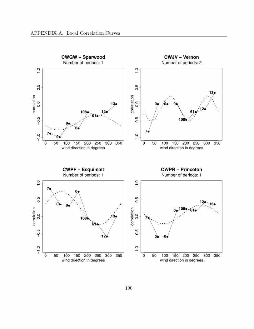
APPENDIX A. Local Correlation Curves
●
●
●
●
●
●
●
●
0 50 100 150 200 250 300 350
−1.0
−0.5
0.0
0.5
1.0
wind direction in degrees
corre
latio
n
CWGW − SparwoodNumber of periods: 1
70
00
10861
12
13
●
● ● ●
●
●
●
●
0 50 100 150 200 250 300 350−1
.0−0
.50.
00.
51.
0
wind direction in degrees
corre
latio
n
CWJV − VernonNumber of periods: 2
7
0 0 0
108
61 12
13
●
●●
●
●
●
●
●
0 50 100 150 200 250 300 350
−1.0
−0.5
0.0
0.5
1.0
wind direction in degrees
corre
latio
n
CWPF − EsquimaltNumber of periods: 1
7
0 0
0
10861
12
13●
● ●
●●
●
●●
0 50 100 150 200 250 300 350
−1.0
−0.5
0.0
0.5
1.0
wind direction in degrees
corre
latio
n
CWPR − PrincetonNumber of periods: 1
7
0 0
0 108 61
12 13
100

APPENDIX A. Local Correlation Curves
●
●
● ● ●
●
●
●
0 50 100 150 200 250 300 350
−1.0
−0.5
0.0
0.5
1.0
wind direction in degrees
corre
latio
n
CWVF − Sand HeadsNumber of periods: 1
25
57 29 49
103
52 ●
●
●
●
●
●
●
●
0 50 100 150 200 250 300 350
−1.0
−0.5
0.0
0.5
1.0
wind direction in degrees
corre
latio
n
CWVV − Victoria HartlandNumber of periods: 1
25
5
7
29
49103
5
2
●
●
●
●
●
●●
●
0 50 100 150 200 250 300 350
−1.0
−0.5
0.0
0.5
1.0
wind direction in degrees
corre
latio
n
CWZG − Banff MarineNumber of periods: 1
25
57
29 49
103 5 2
●
●
●
●
●
●
●
●
0 50 100 150 200 250 300 350
−1.0
−0.5
0.0
0.5
1.0
wind direction in degrees
corre
latio
n
CWZO − Kelp ReefNumber of periods: 1
25
5
7
2949
103
5
2
101
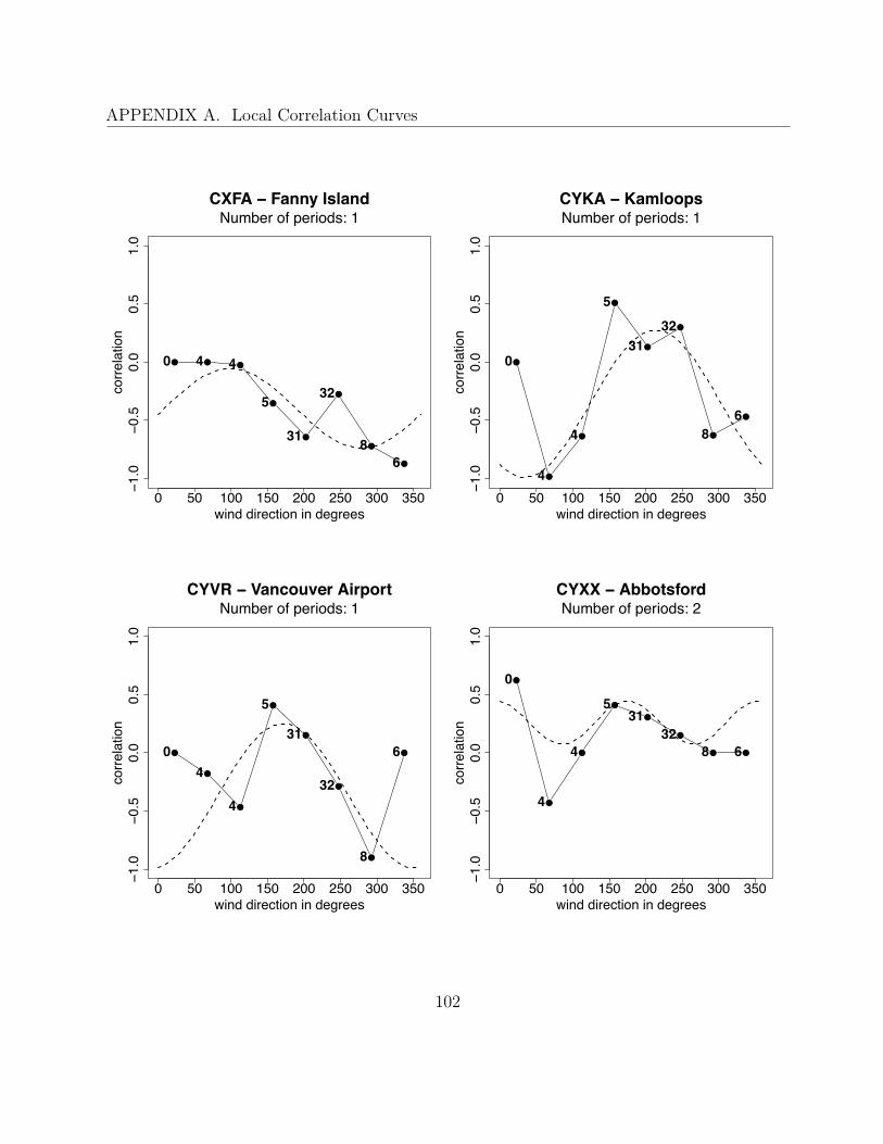
APPENDIX A. Local Correlation Curves
● ● ●
●
●
●
●
●
0 50 100 150 200 250 300 350
−1.0
−0.5
0.0
0.5
1.0
wind direction in degrees
corre
latio
n
CXFA − Fanny IslandNumber of periods: 1
0 4 4
5
31
32
86
●
●
●
●
●
●
●
●
0 50 100 150 200 250 300 350−1
.0−0
.50.
00.
51.
0
wind direction in degrees
corre
latio
n
CYKA − KamloopsNumber of periods: 1
0
4
4
5
3132
86
●
●
●
●
●
●
●
●
0 50 100 150 200 250 300 350
−1.0
−0.5
0.0
0.5
1.0
wind direction in degrees
corre
latio
n
CYVR − Vancouver AirportNumber of periods: 1
04
4
5
31
32
8
6
●
●
●
●
●
●
● ●
0 50 100 150 200 250 300 350
−1.0
−0.5
0.0
0.5
1.0
wind direction in degrees
corre
latio
n
CYXX − AbbotsfordNumber of periods: 2
0
4
4
531
328 6
102

APPENDIX A. Local Correlation Curves
●
● ● ●
●
●
●
●
0 50 100 150 200 250 300 350
−1.0
−0.5
0.0
0.5
1.0
wind direction in degrees
corre
latio
n
CYYF − PentictonNumber of periods: 2
12
7 9 22
24
30
1
3
●
●
●
●
● ●●
●
0 50 100 150 200 250 300 350
−1.0
−0.5
0.0
0.5
1.0
wind direction in degrees
corre
latio
n
CYYJ − Victoria AirportNumber of periods: 1
12
79
22
24 30 1
3
●
●
●
●
●
●●
●
0 50 100 150 200 250 300 350
−1.0
−0.5
0.0
0.5
1.0
wind direction in degrees
corre
latio
n
CYZT − Port HardyNumber of periods: 2
12
7
922
24 30 1 3
●
●
●
●
●
●
●
●
0 50 100 150 200 250 300 350
−1.0
−0.5
0.0
0.5
1.0
wind direction in degrees
corre
latio
n
KAAT − AlturasNumber of periods: 2
12
79
2224
301
3
103

APPENDIX A. Local Correlation Curves
●
● ●●
● ●●
●
0 50 100 150 200 250 300 350
−1.0
−0.5
0.0
0.5
1.0
wind direction in degrees
corre
latio
n
KACV − ArcataNumber of periods: 1
12
0 0 14
49 88 1415
●
● ●
●
●
● ● ●
0 50 100 150 200 250 300 350−1
.0−0
.50.
00.
51.
0
wind direction in degrees
corre
latio
n
KALW − Walla WallaNumber of periods: 1
12
0 0
14
49
88 14 15
●
●
●
●
●
●
●
●
0 50 100 150 200 250 300 350
−1.0
−0.5
0.0
0.5
1.0
wind direction in degrees
corre
latio
n
KAST − AstoriaNumber of periods: 2
12
0
0
14
4988
14
15
● ●
●
●
●●
●
●
0 50 100 150 200 250 300 350
−1.0
−0.5
0.0
0.5
1.0
wind direction in degrees
corre
latio
n
KAWO − ArlingtonNumber of periods: 2
12 0
0
14
49 88
14
15
104

APPENDIX A. Local Correlation Curves
● ● ●
●
●
●
●
●
0 50 100 150 200 250 300 350
−1.0
−0.5
0.0
0.5
1.0
wind direction in degrees
corre
latio
n
KBFI − Seattle Boeing FieldNumber of periods: 2
22 2 32
51
1111
17103
●
●
●
●
●
●
●
●
0 50 100 150 200 250 300 350
−1.0
−0.5
0.0
0.5
1.0
wind direction in degrees
corre
latio
n
KBKE − BakerNumber of periods: 2
22
2
3251
11
11
17
103
●
●
●
●
●
●
●
●
0 50 100 150 200 250 300 350
−1.0
−0.5
0.0
0.5
1.0
wind direction in degrees
corre
latio
n
KBLI − BellinghamNumber of periods: 1
22
2
32
51
11
11
17
103
●
●
●
●
●
●
●
●
0 50 100 150 200 250 300 350
−1.0
−0.5
0.0
0.5
1.0
wind direction in degrees
corre
latio
n
KBNO − BurnsNumber of periods: 1
22
232
51
11
11
17
103
105
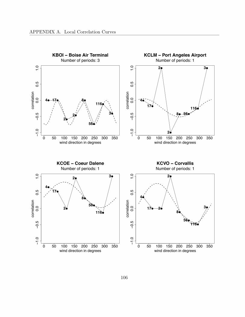
APPENDIX A. Local Correlation Curves
● ●
●
●
●
●
●
●
0 50 100 150 200 250 300 350
−1.0
−0.5
0.0
0.5
1.0
wind direction in degrees
corre
latio
n
KBOI − Boise Air TerminalNumber of periods: 3
4 17
22
8
56
116
3
●
●
●
●
● ●
●
●
0 50 100 150 200 250 300 350−1
.0−0
.50.
00.
51.
0
wind direction in degrees
corre
latio
n
KCLM − Port Angeles AirportNumber of periods: 1
417
2
2
8 56116
3
●
●
●
●
●
●
●
●
0 50 100 150 200 250 300 350
−1.0
−0.5
0.0
0.5
1.0
wind direction in degrees
corre
latio
n
KCOE − Coeur DaleneNumber of periods: 1
417
2
2
8
56
116
3
●
● ●
●
●
●
●
●
0 50 100 150 200 250 300 350
−1.0
−0.5
0.0
0.5
1.0
wind direction in degrees
corre
latio
n
KCVO − CorvallisNumber of periods: 1
4
17 2
2
8
56116
3
106
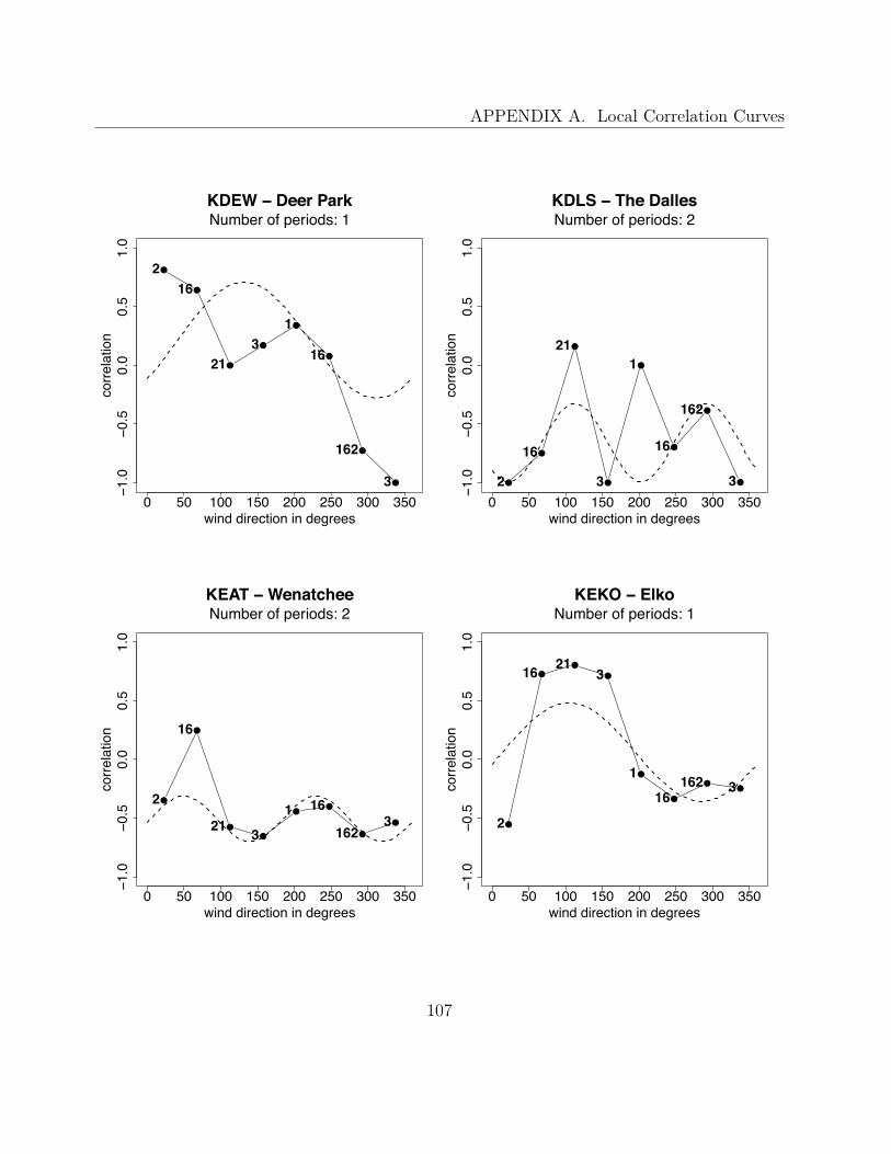
APPENDIX A. Local Correlation Curves
●
●
●
●
●
●
●
●
0 50 100 150 200 250 300 350
−1.0
−0.5
0.0
0.5
1.0
wind direction in degrees
corre
latio
n
KDEW − Deer ParkNumber of periods: 1
216
213
1
16
162
3 ●
●
●
●
●
●
●
●
0 50 100 150 200 250 300 350
−1.0
−0.5
0.0
0.5
1.0
wind direction in degrees
corre
latio
n
KDLS − The DallesNumber of periods: 2
2
16
21
3
1
16
162
3
●
●
●●
●●
●
●
0 50 100 150 200 250 300 350
−1.0
−0.5
0.0
0.5
1.0
wind direction in degrees
corre
latio
n
KEAT − WenatcheeNumber of periods: 2
2
16
21 3
1 16
1623 ●
●●
●
●
●
●●
0 50 100 150 200 250 300 350
−1.0
−0.5
0.0
0.5
1.0
wind direction in degrees
corre
latio
n
KEKO − ElkoNumber of periods: 1
2
16 213
1
16162 3
107

APPENDIX A. Local Correlation Curves
●
● ●
●
● ●
● ●
0 50 100 150 200 250 300 350
−1.0
−0.5
0.0
0.5
1.0
wind direction in degrees
corre
latio
n
KELN − EllensburgNumber of periods: 1
20
10 0
21
85 4336 2
●
●
●
●
●
●
●
●
0 50 100 150 200 250 300 350−1
.0−0
.50.
00.
51.
0
wind direction in degrees
corre
latio
n
KEPH − EphrataNumber of periods: 2
20
10
021
85
43
36
2
●
● ● ●
●
●
●
●
0 50 100 150 200 250 300 350
−1.0
−0.5
0.0
0.5
1.0
wind direction in degrees
corre
latio
n
KEUG − EugeneNumber of periods: 2
20
10 0 2185
43
36
2● ●
●
●
●
●
●●
0 50 100 150 200 250 300 350
−1.0
−0.5
0.0
0.5
1.0
wind direction in degrees
corre
latio
n
KEUL − CaldwellNumber of periods: 2
20 10
0
21
85
4336 2
108
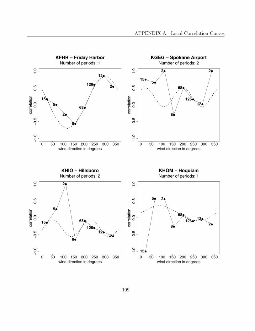
APPENDIX A. Local Correlation Curves
●
●
●
●
●
●
●
●
0 50 100 150 200 250 300 350
−1.0
−0.5
0.0
0.5
1.0
wind direction in degrees
corre
latio
n
KFHR − Friday HarborNumber of periods: 1
155
2
8
68
126
12
2
●
●
●
●
●
●
●
●
0 50 100 150 200 250 300 350
−1.0
−0.5
0.0
0.5
1.0
wind direction in degrees
corre
latio
n
KGEG − Spokane AirportNumber of periods: 2
155
2
8
68
12612
2
●
●
●
●
●
●
●
●
0 50 100 150 200 250 300 350
−1.0
−0.5
0.0
0.5
1.0
wind direction in degrees
corre
latio
n
KHIO − HillsboroNumber of periods: 2
15
5
2
8
68126
122
●
● ●
●
●
●●
●
0 50 100 150 200 250 300 350
−1.0
−0.5
0.0
0.5
1.0
wind direction in degrees
corre
latio
n
KHQM − HoquiamNumber of periods: 1
15
5 2
8
68126 12
2
109

APPENDIX A. Local Correlation Curves
●
●
●
●
●
●
●●
0 50 100 150 200 250 300 350
−1.0
−0.5
0.0
0.5
1.0
wind direction in degrees
corre
latio
n
KHRI − HermistonNumber of periods: 1
10
1
5
54
34
37
86 35
●
●
●
●
●●
●
●
0 50 100 150 200 250 300 350−1
.0−0
.50.
00.
51.
0
wind direction in degrees
corre
latio
n
KKLS − KelsoNumber of periods: 1
10
1
5
54
34 37
86
35
●
●
●
●
●
●
●
●
0 50 100 150 200 250 300 350
−1.0
−0.5
0.0
0.5
1.0
wind direction in degrees
corre
latio
n
KLGD − La GrandeNumber of periods: 1
101
5
54
34
37
8635
●
●
●
●
●
●
●
●
0 50 100 150 200 250 300 350
−1.0
−0.5
0.0
0.5
1.0
wind direction in degrees
corre
latio
n
KLKV − LakeviewNumber of periods: 2
10
1
5
5434
37
86
35
110

APPENDIX A. Local Correlation Curves
●
●
●
●
●●
●
●
0 50 100 150 200 250 300 350
−1.0
−0.5
0.0
0.5
1.0
wind direction in degrees
corre
latio
n
KLMT − Klamath FallsNumber of periods: 1
6
51
8
16 23
98
41●
●
●
●
●
●
●
●
0 50 100 150 200 250 300 350
−1.0
−0.5
0.0
0.5
1.0
wind direction in degrees
corre
latio
n
KLWS − LewistonNumber of periods: 1
6
5
18
16
23
98
41
●
● ●
●
●
●
●●
0 50 100 150 200 250 300 350
−1.0
−0.5
0.0
0.5
1.0
wind direction in degrees
corre
latio
n
KMFR − MedfordNumber of periods: 1
6
5 1
816
2398 41
●●
●
●
●
●
●
●
0 50 100 150 200 250 300 350
−1.0
−0.5
0.0
0.5
1.0
wind direction in degrees
corre
latio
n
KMHS − Mount ShastaNumber of periods: 3
6 5
1
8
16
23
98
41
111

APPENDIX A. Local Correlation Curves
●
● ● ●
●
●
●
●
0 50 100 150 200 250 300 350
−1.0
−0.5
0.0
0.5
1.0
wind direction in degrees
corre
latio
n
KMLP − Mullan PassNumber of periods: 1
38
3 0 5
57
61
45
25●
●
●
●
●
● ●
●
0 50 100 150 200 250 300 350−1
.0−0
.50.
00.
51.
0
wind direction in degrees
corre
latio
n
KMMV − McMinnvilleNumber of periods: 1
38
30
5
5761 45
25
●
●
●● ●
●
●
●
0 50 100 150 200 250 300 350
−1.0
−0.5
0.0
0.5
1.0
wind direction in degrees
corre
latio
n
KMWH − Moses LakeNumber of periods: 1
38
3
0 5 57 6145
25
●
● ● ●
●
●
●
●
0 50 100 150 200 250 300 350
−1.0
−0.5
0.0
0.5
1.0
wind direction in degrees
corre
latio
n
KMYL − McCallNumber of periods: 1
383 0 5
5761
45
25
112
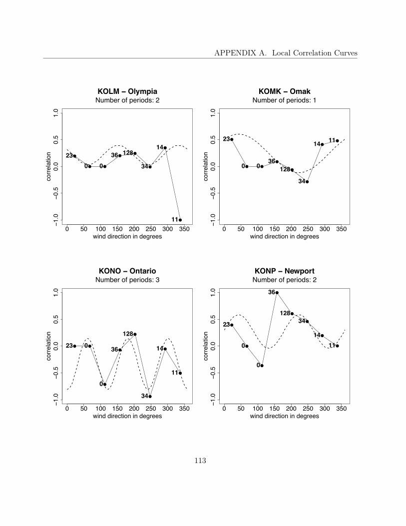
APPENDIX A. Local Correlation Curves
●
● ●
●●
●
●
●
0 50 100 150 200 250 300 350
−1.0
−0.5
0.0
0.5
1.0
wind direction in degrees
corre
latio
n
KOLM − OlympiaNumber of periods: 2
230 0
36 128
34
14
11
●
● ●
●
●
●
●●
0 50 100 150 200 250 300 350
−1.0
−0.5
0.0
0.5
1.0
wind direction in degrees
corre
latio
n
KOMK − OmakNumber of periods: 1
23
0 036
128
34
14 11
● ●
●
●
●
●
●
●
0 50 100 150 200 250 300 350
−1.0
−0.5
0.0
0.5
1.0
wind direction in degrees
corre
latio
n
KONO − OntarioNumber of periods: 3
23 0
0
36
128
34
14
11
●
●
●
●
●
●
●
●
0 50 100 150 200 250 300 350
−1.0
−0.5
0.0
0.5
1.0
wind direction in degrees
corre
latio
n
KONP − NewportNumber of periods: 2
23
0
0
36
12834
1411
113
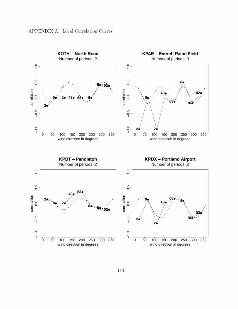
APPENDIX A. Local Correlation Curves
●
● ● ● ● ●
● ●
0 50 100 150 200 250 300 350
−1.0
−0.5
0.0
0.5
1.0
wind direction in degrees
corre
latio
n
KOTH − North BendNumber of periods: 2
2
0 2 48 68 8
16 102
●
●
●
●
●
●
●
●
0 50 100 150 200 250 300 350−1
.0−0
.50.
00.
51.
0
wind direction in degrees
corre
latio
n
KPAE − Everett Paine FieldNumber of periods: 3
2
0
2
48
68
8
16
102
●
● ●
●●
●●
●
0 50 100 150 200 250 300 350
−1.0
−0.5
0.0
0.5
1.0
wind direction in degrees
corre
latio
n
KPDT − PendletonNumber of periods: 2
20 2
48 68
8 16 102
●
●
●
●
●●
●
●
0 50 100 150 200 250 300 350
−1.0
−0.5
0.0
0.5
1.0
wind direction in degrees
corre
latio
n
KPDX − Portland AirportNumber of periods: 2
2
0
2
4868 8
16102
114
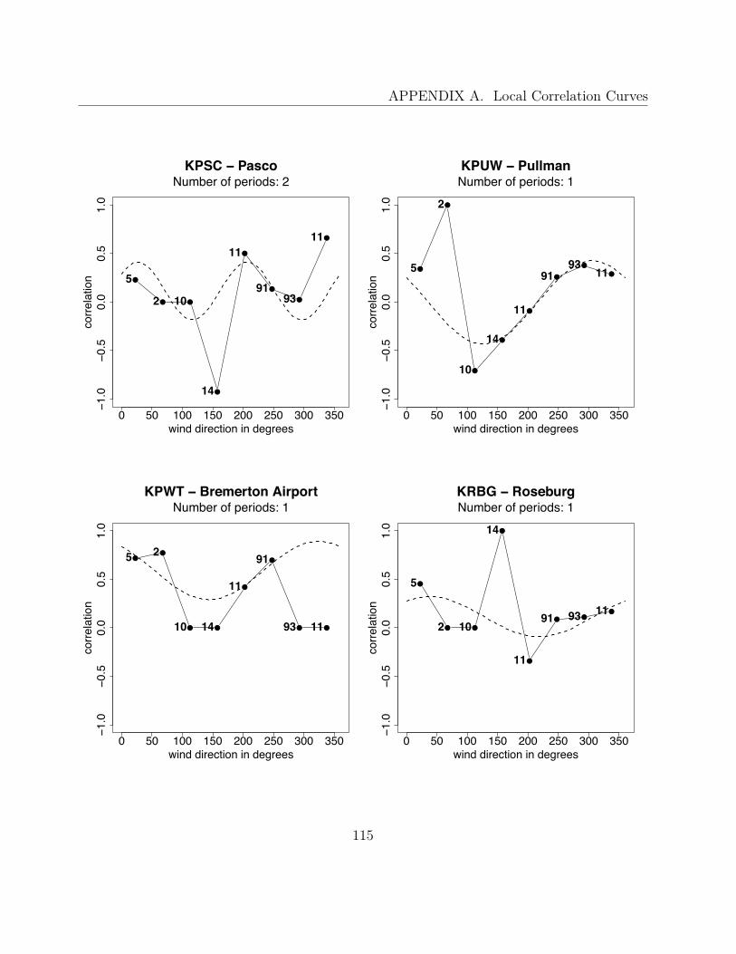
APPENDIX A. Local Correlation Curves
●
● ●
●
●
●
●
●
0 50 100 150 200 250 300 350
−1.0
−0.5
0.0
0.5
1.0
wind direction in degrees
corre
latio
n
KPSC − PascoNumber of periods: 2
5
2 10
14
11
9193
11
●
●
●
●
●
●
●
●
0 50 100 150 200 250 300 350
−1.0
−0.5
0.0
0.5
1.0
wind direction in degrees
corre
latio
n
KPUW − PullmanNumber of periods: 1
5
2
10
14
11
9193
11
●●
● ●
●
●
● ●
0 50 100 150 200 250 300 350
−1.0
−0.5
0.0
0.5
1.0
wind direction in degrees
corre
latio
n
KPWT − Bremerton AirportNumber of periods: 1
5 2
10 14
11
91
93 11
●
● ●
●
●
● ●●
0 50 100 150 200 250 300 350
−1.0
−0.5
0.0
0.5
1.0
wind direction in degrees
corre
latio
n
KRBG − RoseburgNumber of periods: 1
5
2 10
14
11
91 93 11
115

APPENDIX A. Local Correlation Curves
●
● ●
●
●
●
●
●
0 50 100 150 200 250 300 350
−1.0
−0.5
0.0
0.5
1.0
wind direction in degrees
corre
latio
n
KRDM − RedmondNumber of periods: 1
10
0 2
5
91
312
60
●
●
●
●
●
●
●
●
0 50 100 150 200 250 300 350−1
.0−0
.50.
00.
51.
0
wind direction in degrees
corre
latio
n
KRNT − RentonNumber of periods: 2
10
0
2
5
9131
2
60
●● ●
●
●
●
●
●
0 50 100 150 200 250 300 350
−1.0
−0.5
0.0
0.5
1.0
wind direction in degrees
corre
latio
n
KSEA − Sea−Tac AirportNumber of periods: 1
10 0 2
5
9131
2
60●
●
●
● ●
●
●
●
0 50 100 150 200 250 300 350
−1.0
−0.5
0.0
0.5
1.0
wind direction in degrees
corre
latio
n
KSFF − Spokane Felts FieldNumber of periods: 1
100
2
5 91
312
60
116

APPENDIX A. Local Correlation Curves
●
●
●
●
●
●
●
●
0 50 100 150 200 250 300 350
−1.0
−0.5
0.0
0.5
1.0
wind direction in degrees
corre
latio
n
KSHN − SheltonNumber of periods: 2
45
20
7
81
46
2746 ●
●
●
●●
● ●
●
0 50 100 150 200 250 300 350
−1.0
−0.5
0.0
0.5
1.0
wind direction in degrees
corre
latio
n
KSLE − SalemNumber of periods: 2
45
2
07 81
46 27
46
● ●
●
●
●
●
●
●
0 50 100 150 200 250 300 350
−1.0
−0.5
0.0
0.5
1.0
wind direction in degrees
corre
latio
n
KSMP − Stampede PassNumber of periods: 2
45 20
7
81
4627
46
●
●●
● ●
●
● ●
0 50 100 150 200 250 300 350
−1.0
−0.5
0.0
0.5
1.0
wind direction in degrees
corre
latio
n
KSPB − ScappooseNumber of periods: 2
45
2 0
7 81
46
27 46
117

APPENDIX A. Local Correlation Curves
●
●
●
●
●
●
●
●
0 50 100 150 200 250 300 350
−1.0
−0.5
0.0
0.5
1.0
wind direction in degrees
corre
latio
n
KSXT − Sexton SummitNumber of periods: 1
39
1
0
0
7686
20
●● ● ●
●●
●
●
0 50 100 150 200 250 300 350−1
.0−0
.50.
00.
51.
0
wind direction in degrees
corre
latio
n
KTIW − Tacoma Narrows AirportNumber of periods: 1
39 1 0 0 76 86
2
0
●
●
●
●
●
●
●
●
0 50 100 150 200 250 300 350
−1.0
−0.5
0.0
0.5
1.0
wind direction in degrees
corre
latio
n
KTTD − TroutdaleNumber of periods: 1
39
1
0
0
76
86
20
●
●●
●
●
●
●●
0 50 100 150 200 250 300 350
−1.0
−0.5
0.0
0.5
1.0
wind direction in degrees
corre
latio
n
KUAO − AuroraNumber of periods: 1
39
1 0
0
7686
2 0
118

APPENDIX A. Local Correlation Curves
●
●
●
●
●
●
●
●
0 50 100 150 200 250 300 350
−1.0
−0.5
0.0
0.5
1.0
wind direction in degrees
corre
latio
n
KUIL − QuillayuteNumber of periods: 1
4
19
6
4
53
3719
51
●
●
●
●
●
●
●●
0 50 100 150 200 250 300 350
−1.0
−0.5
0.0
0.5
1.0
wind direction in degrees
corre
latio
n
KVUO − VancouverNumber of periods: 2
4
196
4
53
37
1951
●
●
●
●
●
●
●
●
0 50 100 150 200 250 300 350
−1.0
−0.5
0.0
0.5
1.0
wind direction in degrees
corre
latio
n
KYKM − YakimaNumber of periods: 3
4
19
6
4
53
37
19
51
119

Appendix B
List of Notation for Chapter 4
Ui Forecast of the ith ensemble member, for wind component U
Vi Forecast of the ith ensemble member, for wind component V
U Ensemble mean for wind component U
V Ensemble mean for wind component V
SU/S2U Ensemble standard deviation and variance for wind component U
SV /S2V Ensemble standard deviation and variance for wind component V
x Observed wind vector
U Observed value for wind component U
V Observed value for wind component V
µ Predictive mean vector
µU Predictive mean for wind component U
µV Predictive mean for wind component V
Σ Predictive variance-covariance matrix
σU/σ2U Predictive standard deviation and variance for wind component U
120

APPENDIX B. List of Notation for Chapter 4
σV /σ2V Predictive standard deviation and variance for wind component V
ρ Predictive correlation coefficient of the wind components
θ Predictive wind direction, computed from the predictive mean
w Observed wind speed
M Ensemble size
m Length of training period in days
s Location for which the forecasts is issued
t Valid time of the forecast
121


Bibliography
Anderson, J. L. (1996) A method for producing and evaluating probabilistic forecasts fromensemble model integrations. Journal of Climate, 9, 1518–1530.
Baars, J. (2005) Observations QC documentation. Available at http://www.atmos.washington.edu/mm5rt/qc_obs/qc_doc.html.
Baldauf, M., A. Seifert, J. Förstner, D. Majewski, M. Raschendorfer and T. Reinhardt(2011) Operational convective-scale numerical weather prediction with the COSMO model:description and sensitivities. To appear in Monthly Weather Review.
Bao, L., T. Gneiting, E. P. Grimit, P. Guttorp and A. E. Raftery (2010) Bias correction andBayesian model averaging for ensemble forecasts of surface wind direction. Monthly WeatherReview, 138, 1811–1821.
Bernardo, J. M. (1979) Expected information as expected utility. Annals of Statistics, 7,686–690.
Berrocal, V. J., A. E. Raftery and T. Gneiting (2007) Combining spatial statistical andensemble information in probabilistic weather forecasts. Monthly Weather Review, 135,1386–1402.
Bröcker, J. and L. A. Smith (2007) Scoring probabilistic forecasts: The importance of beingproper. Weather and Forecasting, 22, 382–388.
Dawid, A. (1984) Statistical theory: The prequential approach. Journal of the Royal StatisticalSociety Series A, 147, 278–292.
123

BIBLIOGRAPHY
Delle Monache, L., J. P. Hacker, Y. Zhou, X. Deng and R. B. Stull (2006) Probabilistic aspectsof meteorological and ozone regional ensemble forecasts. Journal of Geophysical Research,111, D24307, doi:10.1029/2005JD006917.
Diebold, F. X., T. A. Gunther and A. S. Tay (1998) Evaluating density forecasts withapplications to financial risk management. International Economic Review, 39, 863–883.
Eckel, F. A. and C. F. Mass (2005) Aspects of effective mesoscale, short-range ensembleforecasting. Weather and Forecasting, 20, 328–350.
Gigerenzer, G., R. Hertwig, E. van den Broek, B. Fasolo and K. V. Katsikopoulos (2005)"A 30% chance of rain tomorrow": How does the public understand probabilistic weatherforecasts? Risk Analysis, 25, 623–9.
Glahn, H. R. and D. A. Lowry (1972) The use of model output statistics (MOS) in objectiveweather forecasting. Journal of Applied Meteorology, 11, 1203–1211.
Gneiting, T. (2008) Editorial: Probabilistic forecasting. Journal of the Royal Statistical Society:Series A (Statistics in Society), 171, 319–321.
Gneiting, T. (2011) Making and evaluating point forecasts. Journal of the American StatisticalAssociation, 106, 746–762.
Gneiting, T., F. Balabdaoui and A. E. Raftery (2007) Probabilistic forecasts, calibration andsharpness. Journal of the Royal Statistical Society: Series B (Statistical Methodology), 69,243–268.
Gneiting, T. and A. E. Raftery (2005) Weather forecasting with ensemble methods. Science,310, 248.
Gneiting, T. and A. E. Raftery (2007) Strictly proper scoring rules, prediction, and estimation.Journal of the American Statistical Association, 102, 359–378.
Gneiting, T., A. E. Raftery, A. H. Westveld and T. Goldman (2005) Calibrated probabilisticforecasting using ensemble model output statistics and minimum CRPS estimation. MonthlyWeather Review, 133, 1098–1118.
124

BIBLIOGRAPHY
Gneiting, T., L. I. Stanberry, E. P. Grimit, L. Held and N. A. Johnson (2008) Assessingprobabilistic forecasts of multivariate quantities, with an application to ensemble predictionsof surface winds. Test, 17, 211–235.
Good, I. (1952) Rational decisions. Journal of the Royal Statistical Society Series B, 14,107–114.
Grimit, E. and C. Mass (2002) Initial results of a mesoscale short-range ensemble forecastingsystem over the Pacific Northwest. Weather and Forecasting, 17, 192–205.
Grimit, E. P. (2001) Implementation and Evaluation of a Mesoscale Short-Range EnsembleForecasting System over the Pacific Northwest. Master’s thesis, Department of AtmosphericSciences, University of Washington.
Hamill, T. M. (2001) Interpretation of rank histograms for verifying ensemble forecasts.Monthly Weather Review, 129, 550–560.
Hamill, T. M. and S. J. Colucci (1997) Verification of Eta-RSM short-range ensemble forecasts.Monthly Weather Review, 125, 1312–1327.
Jolliffe, I. T. (2008) Comments on: Assessing probabilistic forecasts of multivariate quantities,with an application to ensemble predictions of surface winds. Test, 17, 249–250.
Leutbecher, M. and T. Palmer (2008) Ensemble forecasting. Journal of Computational Physics,227, 3515–3539.
Matheson, J. E. and R. L. Winkler (1976) Scoring rules for continuous probability distributions.Management Science, 22, 1087–1096.
National Weather Service (1998) Automated Surface Observing System (ASOS) User’s Guide.Available at http://www.weather.gov/asos/aum-toc.pdf.
Palmer, T. (2002) The economic value of ensemble forecasts as a tool for risk assessment: fromdays to decades. Quarterly Journal of the Royal Meteorological Society, 128, 747–774.
125

BIBLIOGRAPHY
Pinson, P. (2011) Adaptive calibration of (u ,v)-wind ensemble forecasts. Available at http://www2.imm.dtu.dk/~pp/docs/pinson11_uvcalibrev.pdf.
R Development Core Team (2011) R: A Language and Environment for Statistical Computing.Available at http://www.r-project.org.
Raftery, A. E., T. Gneiting, F. Balabdaoui and M. Polakowski (2005) Using Bayesian modelaveraging to calibrate forecast ensembles. Monthly Weather Review, 133, 1155–1174.
Roulston, M. and L. Smith (2003) Combining dynamical and statistical ensembles. Tellus A,55, 16–30.
Savage, L. J. (1971) Elicitation of personal probabilities and expectations. Journal of theAmerican Statistical Association, 66, 783–801.
Schefzik, R. (2011) Ensemble Copula Coupling. Diploma thesis, Faculty of Mathematics andComputer Science, Heidelberg University.
Sloughter, J. M. (2009) Probabilistic weather forecasting using Bayesian model averag-ing. PhD final presentation, available at http://www.atmos.washington.edu/~cliff/FinalExamination-20090508-JMcLeanSloughter.ppt.
Sloughter, J. M., T. Gneiting and A. E. Raftery (2010) Probabilistic wind speed forecast-ing using ensembles and Bayesian model averaging. Journal of the American StatisticalAssociation, 105, 25–35.
Sloughter, J. M., A. E. Raftery, T. Gneiting and C. Fraley (2007) Probabilistic quantitativeprecipitation forecasting using Bayesian model averaging. Monthly Weather Review, 135,3209–3220.
Talagrand, O., R. Vautard and B. Strauss (1997) Evaluation of probabilistic prediction systems.Proc. Workshop on Predictability, 1–25, Reading, UK, European Centre for Medium-RangeWeather Forecasts.
126
BIBLIOGRAPHY
Thorarinsdottir, T. L. and T. Gneiting (2010) Probabilistic forecasts of wind speed: Ensemblemodel output statistics by using heteroscedastic censored regression. Journal of the RoyalStatistical Society: Series A (Statistics in Society), 173, 371–388.
Thorarinsdottir, T. L. and M. S. Johnson (2011) Probabilistic wind gust forecasting usingnon-homogeneous Gaussian regression. To appear in Monthly Weather Review.
Vardi, Y. and C.-H. Zhang (2000) The multivariate L1-median and associated data depth.Proceedings of the National Academy of Sciences of the United States of America, 97, 1423–6.
Whitaker, J. S. and A. F. Loughe (1998) The relationship between ensemble spread andensemble mean skill. Monthly Weather Review, 126, 3292–3302.
Wilks, D. S. (1995) Statistical Methods in the Atmospheric Sciences. Academic Press.
Winkler, R. L. (1977) Rewarding expertise in probability assessment. Decision Making andChange in Human Affairs (eds. H. Jungermann and G. de Zeeuw), 127–140, Dordrecht:Reidel.
Winkler, R. L. (1996) Scoring rules and the evaluation of probabilities. Test, 5, 1–60.
127


Danksagung
Ich möchte Dr. Thordis L. Thorarinsdottir und Prof. Dr. Tilmann Gneiting dafür danken,dass sie es mir ermöglicht haben mich mit diesem interessanten Thema zu beschäftigen unddass sie mich, nicht nur im Zuge dieser Arbeit, so hervorragend betreut haben. Ein ganzbesonderer Dank gilt meiner Familie, die mich immer uneingeschränkt unterstützt hat und mirmit Rat und Tat zur Seite stand. Zuletzt möchte ich mich noch herzlich bei Kira Feldmannund Corinna Frei für die tolle und produktive Zusammenarbeit bedanken.
129


Erklärung
Hiermit versichere ich, dass ich meine Arbeit selbstständig unter Anleitung verfasst habe, dass
ich keine anderen als die angegebenen Quellen und Hilfsmittel benutzt habe, und dass ich
alle Stellen, die dem Wortlaut oder dem Sinne nach anderen Werken entlehnt sind, durch die
Angabe der Quellen als Entlehnungen kenntlich gemacht habe.
15. September 2011
131