Errare Humanum Est,

In Errore Perservare Stultum?

Eugenio J. Miravete† Ignacio Palacios-Huerta‡

November 3, 2009

Abstract

Theoretical and experimental studies have shown that understanding when and whypeople are attentive and when and why people reason accurately or make systematicmistakes are central questions of the economics of human behavior. We study thesequestions empirically using a micro-panel data set with repeated observations frommore than 2,500 subjects when optional measured tariffs for local telephone callswere introduced in Kentucky in an unanticipated manner. We find that consumersare attentive, tend to underestimate their demand for telephone services and initiallymake mistakes in their choice of tariffs. Yet, they actively engage in tariff switchingin order to reduce the monthly cost of local telephone services despite savings oflow magnitude. Households’ reactions are not symmetric: those who face a morecomplex and cognitively more expensive tariff problem learn more slowly and are morelikely to make mistakes than households that face a simpler tariff choice problem.Appropriately accounting for the effects of dynamic learning, state dependence andunobserved heterogeneity is critical for determining the underlying model of behaviorsupported by the data.

Keywords: State Dependence, Dynamic Discrete Choice Panel Data Models, Delib-eration, Inertia.

JEL Codes: D42, D82, L96.

?

We thank George Akerlof, Andrew Foster, Giuseppe Moscarini, Ralph Siebert, Dan Silverman,Johannes Van Biesebroeck and participants at various seminars and conferences for helpful comments andsuggestions.

†The University of Texas at Austin, Department of Economics, BRB 1.116, 1 University StationC3100, Austin, Texas 78712-0301; and CEPR, London, UK. Phone: 512-232-1718. Fax: 512-471-3510.E–mail: miravete@eco.utexas.edu; http://www.eugeniomiravete.com

‡Department of Management, London School of Economics, Houghton Street, London WC2A 2AE,United Kingdom. Phone: +44 (0) 207-955-5167. E–mail: i.palacios-huerta@lse.ac.uk

:/.../papers/ut12/ut12d05.tex

“It is evident that the rational thing to do is to be irrational

where deliberation and estimation cost more than they are worth.”

Frank Knight (1921), Risk, Uncertainty and Profit.

1 Introduction

Deliberation about economic decisions is a costly activity. Economists, psychologists and

other social scientists have often expressed the idea that decision makers try to achieve a

balance between the benefits of better decision making and the effort costs of decisions.

According, for instance, to Stigler and Becker (1977):

“The making of decisions is costly, and not simply because it is an activity

which some people find unpleasant. In order to make a decision one requires

information, and the information must be analyzed. The costs of searching for

information and of applying the information to a new situation may be such that

habit [and inertia] are sometimes a more efficient way to deal with moderate or

temporary changes in the environment than would be a full, apparently utility-

maximizing decision.”

Similarly, in his Nobel lecture, Tobin (1982) wrote:

“Some decisions by economic agents are reconsidered daily or hourly, while others

are reviewed at intervals a year or longer except when extraordinary events

compel revisions. It would be desirable in principle to allow for differences among

variables in frequencies of change and even to make these frequencies endogenous.

But at present, models of such realism seem beyond the power of our analytical

tools.”

The principles established in these statements seem so fundamental for our under-

standing of human behavior that we would expect they occupy a central role in the theory and

empirics of individual and aggregate decision making. Ideally, various decades of research

would have produced detailed empirical evidence on the type of decision problems where

– 1 –

consumers behave irrationally and the type of problems where they are rational. Further,

we would know how the different types of behaviors depend on the size of information costs,

time costs and perhaps even cognitive costs, as well as on the benefits of better decision

making. And for the problems that consumers are attentive to, we would also have detailed

information on whether subjects are able to reason accurately or tend to make systematic

errors.

The fact, however, is that we are quite far from this ideal. There is an important

recent theoretical literature modelling inattention and its implications in macroeconomics,

and there is also an important theoretical literature on bounded rationality, but to the

best of our knowledge there is no empirical evidence from real life settings that could be

considered to belong to the ideal just described. A number of empirical problems that are

typically insurmountable justify the existing situation. In natural settings there are often

great difficulties:

• in finding individual decision making situations, as opposed to market-level or other

aggregate settings;1

• in determining individuals’ choice and strategy sets;

• in observing and characterizing individuals’ choices precisely;

• in measuring the exact incentive structures that individuals face;

• in carefully addressing selection problems in settings where preferences are endogenous

to the environment or to the behavior of others, and in knowing the determinants of

the endogenous frequency of choices.

In addition to these difficulties, sufficiently rich detailed data on individual choices are

rarely available to allow researches to distinguish the dynamic effects of learning, attention

and information from the effects of unobserved heterogeneity.

1 At the market or other aggregate levels downward-slopping demand functions can be derived evenas consequences of agents’ random choices subject to a budget constraint (e.g., Becker (1962) and Gode andSunder (1993)). As a result, it is generally not possible to distinguish rational from irrational behavior atany level of aggregation.

– 2 –

In this paper we take advantage of a unique opportunity to overcome these obstacles

by studying a natural setting where none of these difficulties are present. South Central Bell

(scb) implemented a detailed tariff experiment for the Kentucky Public Service Commission

in 1986. scb collected demographic and economic information for about 2,500 households

in Louisville. In the Spring of 1986, all households in Kentucky were on mandatory flat

rates, paying $18.70 per month with unlimited local telephone calls. This was the only tariff

available. In July 1986, optional measured services were introduced for the first time in a

way that was unanticipated by consumers. This alternative tariff included a $14.02 monthly

fixed fee, a $5.00 allowance, and a tariff per call that depended on its duration, distance, and

period (time of the day and day of the week). The basic problem that households faced each

month was to determine whether their expected demand for local phone calls next month

would be above or below $19.02, as they would not be billed for the $5.00 allowance unless

their usage level exceeded this limit. That is, an attentive household would have to think

at time t about the expected consumption level at t + 1 and the tariff rate to be applied

to that consumption level; consumption choices will then take place at time t + 1. These

choices were repeated every month and switching tariffs simply required a free phone call. A

rich panel dataset on all the variables and characteristics of interest is available during the

months of April-June and October-December.

The setting includes a number of desirable characteristics for evaluating whether or

not the costs of attention and learning about their own demand were sufficiently high relative

to the expected payoffs so as to induce rational inattention, and whether when subjects pay

attention to their consumption-tariff problem they are able to reason accurately or instead

tend to make systematic mistakes. From an empirical perspective there are no market-level

data, no endogenous preferences, and no learning from others. More precisely:

• We have an individual decision making situation;

• It is trivial to determine strategy sets;

• It is straighforward to observe and characterize individuals’ choices;

• It is easy to measure the incentives and rewards that subjects face;

– 3 –

• The frequency of choices (monthly) is exogenously given; that is, there is no endogenous

timing of decisions;

• Individuals are as close as possible to a tabula rasa since they could not possibly know

their demand prior to the introduction of the alternative tariff because phone calls

were not priced at the margin in the flat rate tariff regime;

• There are no self-selection problems since the penetration of telephone service is ba-

sically 100 percent of the population; in this sense, we have a truly representative

sample;

• Data on many economic and demographic variables, including data on consumers’

expectations about their own consumption, are available for about 2,500 consumers.

Importantly, the data are rich enough to allow us to distinguish the dynamic effects of

learning and incentives from the effects of unobserved heterogeneity.

We estimate a dynamic discrete choice panel data model and find that:

i) Consumers are attentive. No rational inattention is observed, that is consumers’ be-

havior is not characterized by habit or inertia. Instead, they actively engage in tariff

switching in order to reduce the monthly cost of local telephone services;

ii) While consumers facing the new consumption option do make mistakes initially, these

mistakes are not systematic;

iii) Households’ reactions are not symmetric: those who face a more complex and cognitively

more expensive tariff problem learn more slowly and are more likely to make mistakes

than households that face a simpler tariff choice problem.

iv) The magnitude of the differences between the alternative tariff schemes is typically quite

small (about $5-$6 dollars per month), and yet we find that subjects’ responses reacting

to these potential savings are significant and sizeable;

v) We find no evidence of impulsiveness or time-inconsistent choices;

vi) Lastly, the analysis yields an empirical methodological contribution that may be im-

portant for future research. Despite all of the desirable characteristics, the empirical

– 4 –

analysis is far from trivial or straightforward since we need to estimate a binary choice

panel data model with lagged endogenous variables and unobserved heterogeneity. As

is well known, parameter estimates from short panels jointly estimated with individual

fixed effects can be seriously biased and inconsistent when the explanatory variables are

only predetermined as opposed to strictly exogenous (see Arellano and Honore (2001)

for an overview). In our case, the distinction between the sources of persistence turns

out to be critical for determining the underlying model of behavior. Indeed, failing to

control appropriately for the effect of state dependence and unobserved heterogeneity

in our setting yields radically different results: the evidence would support models of

inattentiveness and systematic mistakes when in fact no such support exists.

The remainder of our study proceeds as follows: Section 2 provides a brief literature

review. Section 3 describes in detail the Kentucky tariff experiment including the data set

and some descriptive evidence. Section 4 presents our dynamic discrete choice panel data

model, Section 5 the empirical results, and Section 6 concludes.

2 Literature Review

An important literature has recently explored the potential of modelling rational inattention

in consumers and producers. Reis (2006a) studies the consumption decisions of agents

who face costs of acquiring, absorving and processing information. His model predicts that

aggregate consumption adjusts slowly to shocks, and is able to explain the excess sensitivity

and excess smoothness puzzles.2 Reis (2006b) studies the same problem for producers and

applies the results to a model of inflation. The resulting model fits remarkably well a number

of quantitative facts on post-war inflation. Mankiw and Reis (2002) and Ball, Mankiw, and

Reis (2005) study inattentiveness on the part of price-setting firms and find that the resulting

model matches well the dynamics of inflation and output observed in the data. In the finance

literature, Gabaix and Laibson (2002) assume that investors update their portfolio decisions

infrequently, and show that this can help explain the equity premium puzzle. In the large

2 Sims (2003) and Moscarini (2004) develop alternative models focusing on the information problemthat agents face.

– 5 –

and growing literature on bounded rationality, the importance of deliberation and processing

costs is relevant for most theories that postulate deviations from the assumption of rational,

computationally unconstrained agents.3

With respect to microeconomic empirical evidence, it mainly comes from survey and

experimental studies. Lusardi (1999), Lusardi (2003) and Americks, Caplin, and Leahy

(2003), for instance, find that a significant fraction of survey respondents make financial

plans infrequently and that their behavior has a significant impact on the amount of wealth

that they accumulate. In a survey two months after the announcement by President George

H. Bush of a reduction in the withholding rates for income taxes, Shapiro and Slemrod (1995)

find that about half of the respondents were simply not aware of any change in those rates.

Carroll (2003) uses survey data on inflation expectations to study how news disseminates

throughout the population.

In the experimental literature, Gabaix, Laibson, Moloche, and Weinberg (2006) study

a cognition model which successfully predicts the aggregate empirical regularities of informa-

tion acquisition both within and across experimental games. Costa-Gomes, Crawford, and

Broseta (2006), and Costa-Gomes and Crawford (2006) also study cognition and behavior

in different experimental games.

When subjects are attentive, it is then important to know whether they get it right or

wrong. Conslik (1996) reviews the literature on bounded rationality, including experimental

studies where subjects make errors in updating probabilities, display overconfidence, and

violate several assumptions of unbounded rationality, as well as others where subjects reason

accurately, especially after practice.4 Ultimately, he concludes, the important question is

“when and why people get it right or wrong.”

3 These include the behavioral economics literature (e.g., Sims (1955) and Sims (1987)), the learningand robustness literatures in macroeconomics (i.e., Sargent (1993), Hansen and Sargent (2008)), the gametheory literature (Rubinstein (1998)), the study of the demand for information in Bayesian decision theory(Moscarini and Smith (2001) and Moscarini and Smith (2002)), the determinants of the adoption of rulesof thumb in individual and social learning contexts (Ellison and Fudenberg (1993)), the study of cognitivedissonance and near-rational theories (Akerlof and Dickens (1982) and, Akerlof and Yellen (1982), the studyof business decisions and long-term contracting situations (Bolton and Faure-Grimaud (2005b) and Boltonand Faure-Grimaud (2005a)) and others. On the infinite regress problem, see Savage (1954) and Lipman(1991).

4 Arrow (1987) and Lucas (1987) discuss some limitations of experiments to study bounded rationality.

– 6 –

Thus, these studies show that modeling attention and experimentally studying the

predictions of limited rationality models offer a great deal of promise for improving our

understanding of human decision making. Relative to the existing theoretical, survey and

experimental literature this paper differs by providing what, to the best of our knowledge,

is the first empirical microeconometric study of attentiveness and reasoning in a real world

setting using a large panel dataset of a fully representative sample.

3 Description of the Tariff Experiment

In the second half of 1986, South Central Bell (scb) carried out a detailed tariff experiment

aimed at providing the Kentucky Public Service Commission (kpsc) with evidence in favor

of authorizing the introduction of optional measured tariffs for local telephone service.

Prior to this tariff experiment, in the Spring of 1986, all households in Kentucky were

on mandatory flat rates and scb collected demographic and economic information for about

2,500 households in the local exchange of Louisville. In July of 1986, the tariff was modified in

this city. Customers were given the choice to remain in the previous flat tariff regime—paying

$18.70 per month with unlimited calls—or switch to the new measured service option. The

measured service included a $14.02 monthly fixed fee, a $5.00 allowance,5 and distinguished

among setup, duration, peak periods, and distance.6 Choices could be made every month

and, unless a household indicated to scb otherwise, its current choice of tariff would serve

as default choice for the following month.7 The regulated monopolist also collected monthly

information on usage (number and duration of calls classified by time of the day, day of

the week, and distance within the local loop), and payments during two periods of three

5 Consumers on the measured option were not billed for the first $5.00 unless their usage exceededthat limit. Thus, depending on the accumulated telephone usage over a month, a marginal second ofcommunication could cost $5.00.

6 The tariff differentiated among three periods: peak was from 8 a.m. to 5 p.m. on weekdays;shoulder was between 5 p.m. to 11 p.m. on weekdays and Sunday; and off-peak was any other time. Fordistance band A, measured charges were 2, 1.3, and 0.8 cents for setup and price per minute during the peak,shoulder, and off-peak period, respectively. For distance band B, setup charges were the same but durationwas fixed at 4, 2.6, and 1.6 cents, respectively.

7 Switching tariffs simply required a free phone call to request the change of service.

– 7 –

months, one right before (March-May) and the other (October-December) three months

after the measured tariff option was introduced.8

The data set has a number of valuable features. First, local telephony is a basic

service and its market penetration is close to 100% in the U.S. Thus, there are no potential

self-selection problems or conspicuous consumption considerations that may lead to biased

estimates because of selection into this market. Second, it is safe to rule out any risk

aversion argument that could otherwise explain systematic mistakes regarding the choice of

tariff options because of the low magnitude of the cost differences between the alternative

tariff choices relative to the average household income. Third, it is valuable for the purpose

of the analysis that in addition to demographic and economic variables, scb also collected

information on customers’ own telephone usage expectations in the Spring of 1986, which is

a good approximation of consumers’ own expected satiation levels as marginal tariffs were

nil. Fourth, given that the flat tariff regime means that local calls were not priced at the

margin, households might not be aware, at least not perfectly, of their own actual demand

for local phone calls at the time of the experiment.9

Households receive every month the bill of their consumption. In this sense, the costs

of searching for information are minimal, and thus the costs of deliberation and cognition,

relative to the expected payoffs, would likely be the main, and perhaps only, determinant of

their behavior. Moreover, there is an important asymmetry in the cognitive costs associated

with the problem that households face in the different tariff options. Households in the

measured tariff simply need to compare their actual bill with the $18.70 cost of the alternative

flat tariff in order to ascertain whether or not they made a mistake. Households in the flat

8 This data set has been used in the past. Miravete (2002) identifies the distributions of ex-anteand ex-post telephone usage to evaluate the profit and welfare performance of sequential pricing mecha-nisms consisting of optimal two-part tariffs. Miravete (2003) evaluates the effect of expectations of futureconsumption as stated by consumers and the role of potential savings in driving household tariff switchingbehavior. Miravete (2005) uses the empirical distribution of future expected consumption to evaluate theprofit and welfare performance of sequential pricing mechanisms where options are fully nonlinear tariffs.Finally, Narayanan, Chintagunta, and Miravete (2007) estimate a structural discrete/continuous model ofplan choice and demand of local telephone service where consumers update of future usage expectation isconditioned by the choice of tariff made. Relative to these papers, the present one addresses the issue ofunobserved heterogeneity due to state dependence which translates into testing whether inertia rather thanexperimentation through tariff switching better explains the behavior of households.

9 Measured tariffs were rarely offered in the U.S. before the breakup of AT&T, and local telephoneservices typically consisted of just a flat monthly fee as in Louisville Mitchell and Vogelsang (1991).

– 8 –

tariff option face a much more complex problem: they would need to monitor every phone

call and compute whether the total cost of all of their calls in the month would have been

above or below $19.02 had they subscribed the measured service, where each call is metered

differently depending on their duration, distance, and periods. Clearly, this task is much

more complex and requires a great deal of monitoring effort. Empirically, we would expect

that these asymmetric cognitive costs play an important role in explaining observed behavior.

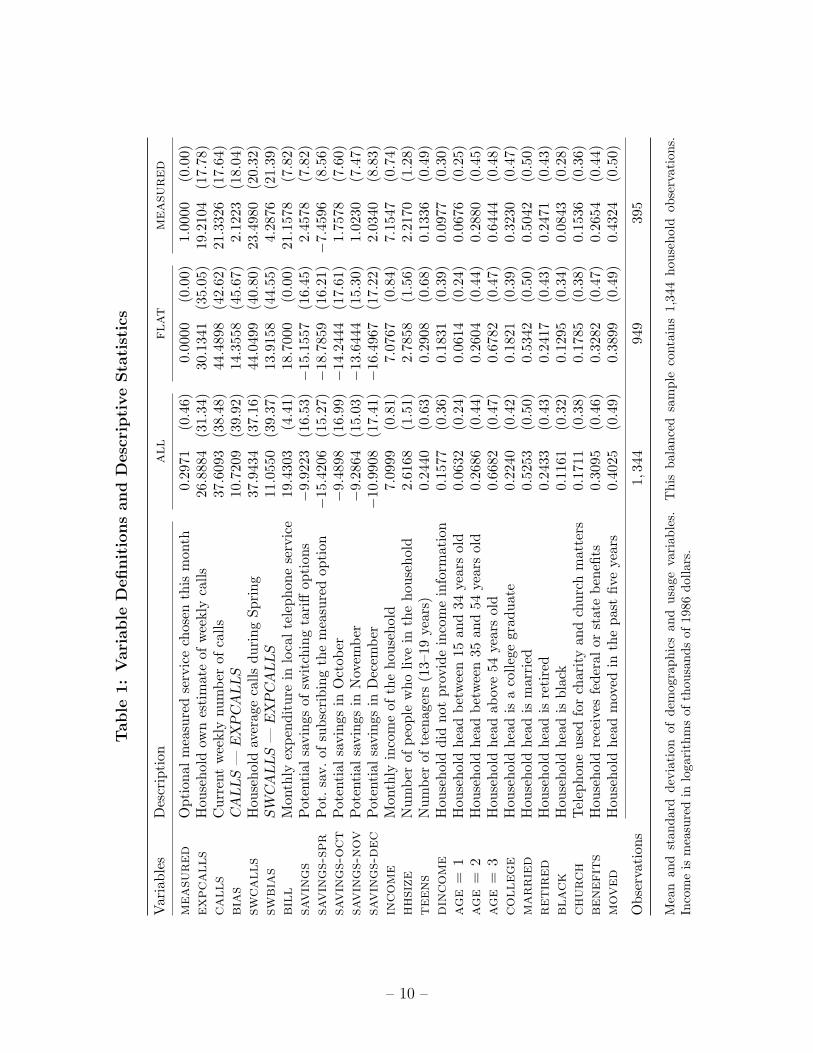
Table 1 defines the different variables and presents basic descriptive statistics for

the whole sample and for two groups of consumers split according to their choice of tariff

in October. Only active consumers were considered and a number of observations with

missing values for some variables were excluded.10 These descriptive statistics initially

suggest that individual heterogeneity in consumption and tariff subscription is important.

Consumers who subscribe to the flat and measured tariffs are in fact quite different.

Households subscribing to the optional flat service, for instance, are on average larger, with

teenagers, and with a lower level of education than those subscribing to the and measured

tariff. Further, they not only differ in their level of local telephone usage —as captured

by calls— but also in their expectations regarding future telephone usage. Subjects tend

to underestimate their demand for telephone services, especially those in the flat tariff in

October.

Despite all the remarkable features of the data, there are two issues that need to

be addressed econometrically. First, about 10% of consumers switched to the optional

measured option when given that possibility. Our sample, however, includes 30% of those

customers. Choice-based sampling bias can easily be dealt with using well known methods

(see Amemiya (1985, §9.5)). All estimates reported in tha analysis take into account this

choice-based sampling as we use the weighting procedure of Lerman and Manski (1977) to

obtain choice-based, heteroskedastic-consistent, standard errors. Second, when the tariff

experiment began in July of 1986, all households were assigned the preexisting flat tariff as

default option. Consumers may learn about their telephone usage profile as they switch tariff

options, and thus, over time, they will differ in experience as summarized by the sequence of

10 Miravete (2002) documents that excluding households with missing information does not lead tobiased results. The only variable with a substantial number of missings is income. In these cases we recodedthe missing observations to the yearly average income of the population in Louisville and also included adummy variable, dincome, to control for non-responses regarding household earnings.

– 9 –

Table

1:

Vari

able

Definitio

ns

and

Desc

riptive

Sta

tist

ics

Var

iabl

esD

escr

ipti

onall

flat

measu

red

measu

red

Opt

iona

lm

easu

red

serv

ice

chos

enth

ism

onth

0.29

71(0

.46)

0.00

00(0

.00)

1.00

00(0

.00)

expcalls

Hou

seho

ldow

nes

tim

ate

ofw

eekl

yca

lls26

.888

4(3

1.34

)30

.134

1(3

5.05

)19

.210

4(1

7.78

)calls

Cur

rent

wee

kly

num

ber

ofca

lls37

.609

3(3

8.48

)44

.489

8(4

2.62

)21

.332

6(1

7.64

)bia

sC

ALLS

—E

XP

CA

LLS

10.7

209

(39.

92)

14.3

558

(45.

67)

2.12

23(1

8.04

)sw

calls

Hou

seho

ldav

erag

eca

llsdu

ring

Spri

ng37

.943

4(3

7.16

)44

.049

9(4

0.80

)23

.498

0(2

0.32

)sw

bia

sSW

CA

LLS

—E

XP

CA

LLS

11.0

550

(39.

37)

13.9

158

(44.

55)

4.28

76(2

1.39

)bil

lM

onth

lyex

pend

itur

ein

loca

lte

leph

one

serv

ice

19.4

303

(4.4

1)18

.700

0(0

.00)

21.1

578

(7.8

2)sa

vin

gs

Pot

enti

alsa

ving

sof

swit

chin

gta

riff

opti

ons

−9.

9223

(16.

53)

−15

.155

7(1

6.45

)2.

4578

(7.8

2)sa

vin

gs-

spr

Pot

.sa

v.of

subs

crib

ing

the

mea

sure

dop

tion

−15

.420

6(1

5.27

)−

18.7

859

(16.

21)

−7.

4596

(8.5

6)sa

vin

gs-

oct

Pot

enti

alsa

ving

sin

Oct

ober

−9.

4898

(16.

99)

−14

.244

4(1

7.61

)1.

7578

(7.6

0)sa

vin

gs-

nov

Pot

enti

alsa

ving

sin

Nov

embe

r−

9.28

64(1

5.03

)−

13.6

444

(15.

30)

1.02

30(7

.47)

savin

gs-

dec

Pot

enti

alsa

ving

sin

Dec

embe

r−

10.9

908

(17.

41)

−16

.496

7(1

7.22

)2.

0340

(8.8

3)in

come

Mon

thly

inco

me

ofth

eho

useh

old

7.09

99(0

.81)

7.07

67(0

.84)

7.15

47(0

.74)

hhsi

ze

Num

ber

ofpe

ople

who

live

inth

eho

useh

old

2.61

68(1

.51)

2.78

58(1

.56)

2.21

70(1

.28)

teens

Num

ber

ofte

enag

ers

(13–

19ye

ars)

0.24

40(0

.63)

0.29

08(0

.68)

0.13

36(0

.49)

din

come

Hou

seho

lddi

dno

tpr

ovid

ein

com

ein

form

atio

n0.

1577

(0.3

6)0.

1831

(0.3

9)0.

0977

(0.3

0)age

=1

Hou

seho

ldhe

adbe

twee

n15

and

34ye

ars

old

0.06

32(0

.24)

0.06

14(0

.24)

0.06

76(0

.25)

age

=2

Hou

seho

ldhe

adbe

twee

n35

and

54ye

ars

old

0.26

86(0

.44)

0.26

04(0

.44)

0.28

80(0

.45)

age

=3

Hou

seho

ldhe

adab

ove

54ye

ars

old

0.66

82(0

.47)

0.67

82(0

.47)

0.64

44(0

.48)

college

Hou

seho

ldhe

adis

aco

llege

grad

uate

0.22

40(0

.42)

0.18

21(0

.39)

0.32

30(0

.47)

marrie

dH

ouse

hold

head

ism

arri

ed0.

5253

(0.5

0)0.

5342

(0.5

0)0.

5042

(0.5

0)retir

ed

Hou

seho

ldhe

adis

reti

red

0.24

33(0

.43)

0.24

17(0

.43)

0.24

71(0

.43)

black

Hou

seho

ldhe

adis

blac

k0.

1161

(0.3

2)0.

1295

(0.3

4)0.

0843

(0.2

8)church

Tel

epho

neus

edfo

rch

arity

and

chur

chm

atte

rs0.

1711

(0.3

8)0.

1785

(0.3

8)0.

1536

(0.3

6)benefit

sH

ouse

hold

rece

ives

fede

ralor

stat

ebe

nefit

s0.

3095

(0.4

6)0.

3282

(0.4

7)0.

2654

(0.4

4)moved

Hou

seho

ldhe

adm

oved

inth

epa

stfiv

eye

ars

0.40

25(0

.49)

0.38

99(0

.49)

0.43

24(0

.50)

Obs

erva

tion

s1,

344

949

395

Mea

nan

dst

anda

rdde

viat

ion

ofde

mog

raph

ics

and

usag

eva

riab

les.

Thi

sba

lanc

edsa

mpl

eco

ntai

ns1,

344

hous

ehol

dob

serv

atio

ns.

Inco

me

ism

easu

red

inlo

gari

thm

sof

thou

sand

sof

1986

dolla

rs.

– 10 –

past tariff choices and usage levels. Testing the economic hypothesis of inertia in the choice

of tariff options requires estimating the effect of past choices on the probability of choosing a

particular tariff option. Obtaining a consistent estimate of these effects requires controlling

for the possibility of unobserved individual heterogeneity due to unobserved sequences of

past choices. To that end we use the semiparametric estimator suggested by Arellano and

Carrasco (2003) in Section 4.

In an attempt to examine whether households tend to choose the ex-post correct tariff

option for their usage level, we first study the pattern of correlation among the decisions

using a simple static model of simultaneous choice of tariff plan and usage level.11 We

estimate the following reduced form model:

y∗j = XΠj + vj , j = 1, 2, (1)

and where, conditional on observed demographics, we assume that:

(v1, v2) ∼ N (0,Σv) ; Σv =

1 ρ

ρ 1

. (2)

These two reduced-form equations are estimated simultaneously as a bivariate probit

model, thus providing an estimate of ρ. In this model y1 = 1 if the household subscribes

the measured tariff, m, and y2 = 1 if the household realizes a low usage level l, defined as a

consumption level below $19.02 when metered according to the measured tariff rates, so that

a positive estimate of ρ can be interpreted as unobservable element inducing the appropriate

tariff choice for each usage level. The model includes the same set of demographic variables in

both equations to control for the effect of observable individual heterogeneity over the tariff

choice and consumption decisions. Data also include household specific information from

the Spring months to control, at least in part, for the accuracy of predictions of individual

future usage. We thus include two dummies to indicate whether consumers significantly over

11 The approach is similar to Chiappori and Salanie (2000) and a significant correlation coefficientin this estimation supports the idea of the existence of asymmetric information beyond the observabledemographics of our data.

– 11 –

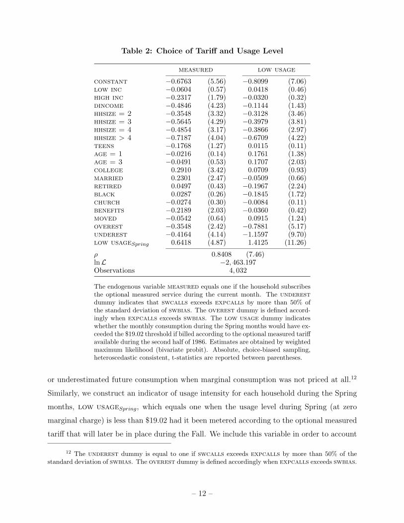
Table 2: Choice of Tariff and Usage Level

measured low usage

constant −0.6763 (5.56) −0.8099 (7.06)low inc −0.0604 (0.57) 0.0418 (0.46)high inc −0.2317 (1.79) −0.0320 (0.32)dincome −0.4846 (4.23) −0.1144 (1.43)hhsize = 2 −0.3548 (3.32) −0.3128 (3.46)hhsize = 3 −0.5645 (4.29) −0.3979 (3.81)hhsize = 4 −0.4854 (3.17) −0.3866 (2.97)hhsize > 4 −0.7187 (4.04) −0.6709 (4.22)teens −0.1768 (1.27) 0.0115 (0.11)age = 1 −0.0216 (0.14) 0.1761 (1.38)age = 3 −0.0491 (0.53) 0.1707 (2.03)college 0.2910 (3.42) 0.0709 (0.93)married 0.2301 (2.47) −0.0509 (0.66)retired 0.0497 (0.43) −0.1967 (2.24)black 0.0287 (0.26) −0.1845 (1.72)church −0.0274 (0.30) −0.0084 (0.11)benefits −0.2189 (2.03) −0.0360 (0.42)moved −0.0542 (0.64) 0.0915 (1.24)overest −0.3548 (2.42) −0.7881 (5.17)underest −0.4164 (4.14) −1.1597 (9.70)low usageSpring 0.6418 (4.87) 1.4125 (11.26)

ρ 0.8408 (7.46)lnL −2, 463.197Observations 4, 032

The endogenous variable measured equals one if the household subscribesthe optional measured service during the current month. The underestdummy indicates that swcalls exceeds expcalls by more than 50% ofthe standard deviation of swbias. The overest dummy is defined accord-ingly when expcalls exceeds swbias. The low usage dummy indicateswhether the monthly consumption during the Spring months would have ex-ceeded the $19.02 threshold if billed according to the optional measured tariffavailable during the second half of 1986. Estimates are obtained by weightedmaximum likelihood (bivariate probit). Absolute, choice-biased sampling,heteroscedastic consistent, t-statistics are reported between parentheses.

or underestimated future consumption when marginal consumption was not priced at all.12

Similarly, we construct an indicator of usage intensity for each household during the Spring

months, low usageSpring, which equals one when the usage level during Spring (at zero

marginal charge) is less than $19.02 had it been metered according to the optional measured

tariff that will later be in place during the Fall. We include this variable in order to account

12 The underest dummy is equal to one if swcalls exceeds expcalls by more than 50% of thestandard deviation of swbias. The overest dummy is defined accordingly when expcalls exceeds swbias.

– 12 –

for any systematic effect of demographics not included in our data on usage. Table 2 reports

the estimates of these reduced form parameters.

The positive estimate of ρ reflects the correlation between the choice of the measured

service and a low demand realization. This suggests that consumers do not appear to make

systematic mistakes when choosing among optional tariffs. Furthermore, estimates of the

effect of demographics suggest that when mistakes are made, it is more likely that they

are made when a household subscribes to the measured service rather than to the flat tariff

option. Consumers on the measured option enjoy a de facto negligible deliberation cost since

they just have to compare their past monthly bill to the cost of the flat option to decide

whether or not to switch tariff plans.

Thus, for instance, larger households tend to subscribe to the flat tariff option and to

realize high usage levels, which is the less expensive option for the telephone usage profile.

At the other end, households whose head holds a college degree are inclined to subscribe

to the measured service option but, conditional on having subscribed the measured option,

they are also more likely to realize a high demand and, thus, to have (incorrectly) chosen

the measured option ex-post. A similar pattern arises for married couples.13

Finally, observe that households with a low usage profile during the Spring months

are more likely to present a low usage pattern in the Fall months as well, and also to choose

(correctly) the measured tariff option. Consumers that either over or underestimated their

future telephone usage quite significantly are less likely to subscribe to the measured option,

but are also far less likely to realize a low usage level. Thus, households who made the largest

absolute forecast errors are among those with very high levels of demand, and thus, they are

more likely to choose the right option by subscribing to the flat tariff.

After this descriptive evidence, we turn toward the more substantive questions: Do

consumers simply stay on their previously chosen tariff because of inertia or rational inat-

tention? Are consumption levels, tariff choices, and the tariff switching that we observe in

the data sufficient to provide evidence that consumers are attentive and respond to potential

savings? What is the role of previous tariff choices and demand realizations on the decision

13 Consumers are classified as having chosen correctly or incorrectly each tariff option ex-post keepingthe usage pattern unchanged, that is independently of price responses. This provides an approximate upperbound to the gains of switching to a different tariff option.

– 13 –

to subscribe to one of the two options? In order to answer these questions we need more

sophisticated econometric methods that allow us to account for state dependence, unobserved

heterogeneity, and dynamic learning. We study such model next.

4 Econometric Model

In this section we first present a semi–parametric, random effects, discrete choice model with

predetermined variables based on the work by Arellano and Carrasco (2003) that controls

for the effect of unobservable heterogeneity due to state dependence. We also discuss why

this model offers useful advantages over the very few alternative approaches available in the

literature. We then implement this model to study the choices of tariffs and consumption

levels. Furthermore, we point out the importance of instrumenting for the lagged endogenous

variables in this model appropriately, and how, ignoring the role of endogeneity may lead to

dramatically opposite results regarding the effect of experience on telephone usage and tariff

choices.

4.1 A Dynamic Discrete Choice Panel Data Model

The model defines conditional probabilities for every possible sequence of realizations of state

variables in order to deal with regressors that are predetermined but not exogenous, such

as the previous choices of tariffs and the past realizations of demand in our setting. Then,

the estimator computes the probability of subscribing to a given tariff along every possible

path of past realizations of demand and subscription decisions. The panel data structure

allows us to identify the effect of individual unobserved heterogeneity since consumers make

different decisions even if they share the same history of realizations of state variables.

The probability of subscribing to a given tariff option, and hence the probability of

switching tariffs in the future, depends on the particular sequence of past choices and past

realizations of demand for each consumer. As consumers choose differently, they accumulate

different experiences and invest differently in information gathering and deliberation efforts.

These experiences in turn change the information set upon which they decide in the future.

For instance, consumers that have previously chosen the measured option may have learned

– 14 –

that their demand is systematically high, so that in the future they will be more likely to

subscribe to the flat tariff option. Consumers that have always remained on the flat tariff

option have accumulated different experiences, which also affects their conditional probability

of renewing their subscription to the flat tariff option. Given that their consumption was

never priced at the margin in any range, these households may have much less knowledge

of their own demand than those that at some point subscribe to the measured service. To

be more specific, the probability of subscribing to a given tariff option may depend on some

intrinsic characteristics of consumers, as well as on their expectation on the realization of

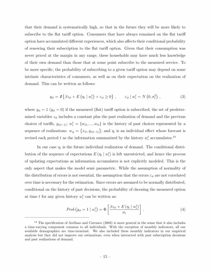
demand. This can be written as follows:

yit = 1I{βzit + E

(ηi | wt

i

)+ εit ≥ 0

}, εit | wt

i ∼ N(0, σ2

t

), (3)

where yit = 1 (yit = 0) if the measured (flat) tariff option is subscribed; the set of predeter-

mined variables zit includes a constant plus the past realization of demand and the previous

choices of tariffs, yi(t−1); wti = {wi1, ..., wit} is the history of past choices represented by a

sequence of realizations: wit ={xit, yi(t−1)

}; and ηi is an individual effect whose forecast is

revised each period t as the information summarized by the history wti accumulates.14

In our case ηi is the future individual realization of demand. The conditional distri-

bution of the sequence of expectations E (ηi | wti) is left unrestricted, and hence the process

of updating expectations as information accumulates is not explicitly modeled. This is the

only aspect that makes the model semi–parametric. While the assumption of normality of

the distribution of errors is not essential, the assumption that the errors εit are not correlated

over time is necessary for the estimation. Since errors are assumed to be normally distributed,

conditional on the history of past decisions, the probability of choosing the measured option

at time t for any given history wti can be written as:

Prob(yit = 1 | wt

i

)= Φ

[βzit + E (ηi | wt

i)

σt

]. (4)

14 The specification of Arellano and Carrasco (2003) is more general in the sense that it also includesa time-varying component common to all individuals. With the exception of monthly indicators, all ouravailable demographics are time-invariant. We also included these monthly indicators in our empiricalanalysis but they did not improve our estimations, even when interacted with past subscription decisionsand past realizations of demand.

– 15 –

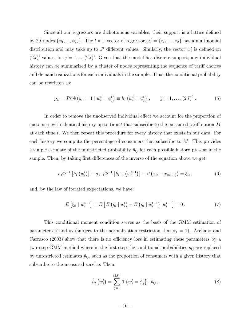
Since all our regressors are dichotomous variables, their support is a lattice defined

by 2J nodes {φ1, ..., φ2J}. The t× 1–vector of regressors zti = {zi1, ..., zit} has a multinomial

distribution and may take up to J t different values. Similarly, the vector wti is defined on

(2J)t values, for j = 1, ..., (2J)t. Given that the model has discrete support, any individual

history can be summarized by a cluster of nodes representing the sequence of tariff choices

and demand realizations for each individuals in the sample. Thus, the conditional probability

can be rewritten as:

pjt = Prob(yit = 1 | wt

i = φtj

)≡ ht

(wt

i = φtj

), j = 1, . . . , (2J)t . (5)

In order to remove the unobserved individual effect we account for the proportion of

customers with identical history up to time t that subscribe to the measured tariff option M

at each time t. We then repeat this procedure for every history that exists in our data. For

each history we compute the percentage of consumers that subscribe to M . This provides

a simple estimate of the unrestricted probability ptj for each possible history present in the

sample. Then, by taking first differences of the inverse of the equation above we get:

σtΦ−1

[ht

(wt

i

)]− σt−1Φ

−1[ht−1

(wt−1

i

)]− β

(xit − xi(t−1)

)= ξit , (6)

and, by the law of iterated expectations, we have:

E[ξit | wt−1

i

]= E

[E

(ηi | wt

i

)− E

(ηi | wt−1

i

)∣∣ wt−1i

]= 0 . (7)

This conditional moment condition serves as the basis of the GMM estimation of

parameters β and σt (subject to the normalization restriction that σ1 = 1). Arellano and

Carrasco (2003) show that there is no efficiency loss in estimating these parameters by a

two–step GMM method where in the first step the conditional probabilities ptj are replaced

by unrestricted estimates ptj, such as the proportion of consumers with a given history that

subscribe to the measured service. Then:

ht

(wt

i

)=

(2J)t∑j=1

1{wt

i = φtj

}· ptj , (8)

– 16 –

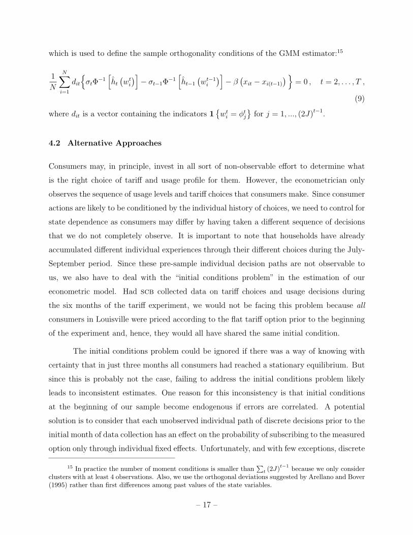
which is used to define the sample orthogonality conditions of the GMM estimator:15

1

N

N∑i=1

dit

{σtΦ

−1[ht

(wt

i

)]− σt−1Φ

−1[ht−1

(wt−1

i

)]− β

(xit − xi(t−1)

) }= 0 , t = 2, . . . , T ,

(9)

where dit is a vector containing the indicators 1{wt

i = φtj

}for j = 1, ..., (2J)t−1.

4.2 Alternative Approaches

Consumers may, in principle, invest in all sort of non-observable effort to determine what

is the right choice of tariff and usage profile for them. However, the econometrician only

observes the sequence of usage levels and tariff choices that consumers make. Since consumer

actions are likely to be conditioned by the individual history of choices, we need to control for

state dependence as consumers may differ by having taken a different sequence of decisions

that we do not completely observe. It is important to note that households have already

accumulated different individual experiences through their different choices during the July-

September period. Since these pre-sample individual decision paths are not observable to

us, we also have to deal with the “initial conditions problem” in the estimation of our

econometric model. Had scb collected data on tariff choices and usage decisions during

the six months of the tariff experiment, we would not be facing this problem because all

consumers in Louisville were priced according to the flat tariff option prior to the beginning

of the experiment and, hence, they would all have shared the same initial condition.

The initial conditions problem could be ignored if there was a way of knowing with

certainty that in just three months all consumers had reached a stationary equilibrium. But

since this is probably not the case, failing to address the initial conditions problem likely

leads to inconsistent estimates. One reason for this inconsistency is that initial conditions

at the beginning of our sample become endogenous if errors are correlated. A potential

solution is to consider that each unobserved individual path of discrete decisions prior to the

initial month of data collection has an effect on the probability of subscribing to the measured

option only through individual fixed effects. Unfortunately, and with few exceptions, discrete

15 In practice the number of moment conditions is smaller than∑

t (2J)t−1 because we only considerclusters with at least 4 observations. Also, we use the orthogonal deviations suggested by Arellano and Bover(1995) rather than first differences among past values of the state variables.

– 17 –

choice models with fixed effects cannot be consistently estimated with finite samples because

of the well-known “incidental parameter problem.16

There are very few results in this literature. The only discrete choice models where the

incidental parameter problem is not present is the conditional maximum likelihood estimator

of Chamberlain (1980) for the logit and Poisson regression. In order to deal with the issue of

state dependence, Honore and Kyriazidou (2000) include one lagged dependent variable but

require that the remaining explanatory variables are strictly exogenous, thus excluding the

possibility of a lagged dependent regressor. This rules out, for instance, that we condition

tariff choices on past usage levels and monthly indicators. Honore and Lewbel (2002) allow

for additional predetermined variables but at the cost of requiring a continuous, strictly

exogenous, explanatory variable that is independent of the individual effects, i.e., we could

condition tariff choices on past usage levels but not the other way around, and the estimates

would be consistent only as long as individual effects are uncorrelated with telephone usage,

an assumption that is highly questionable.

An alternative to the logit specification is the maximum score estimator of Manski

(1987). However, in addition to the strict exogeneity of regressors this estimator also requires

stationarity in order to avoid the initial conditions problem. But stationarity should not be

expected in our sample which contains data collected just three months after the tariff

experiment was launched.

In addition to fixed effects models, research has also contemplated random effects

models in order to deal with unobserved heterogeneity in discrete choice problems, e.g.,

Chamberlain (1984) and Newey (1994). However, beyond the common requirement of strict

exogeneity of regressors, random effects models have the disadvantage that the identification

of parameters depends critically on the arbitrary choice of the conditional distribution of

individual effects by the econometrician. This is not the case in our model because, as

noted earlier, the conditional distribution of the individual effect E (ηi | wti) is not explicitly

modeled.

16 On the statistical problems originated by the initial conditions problem, including its relationshipwith the incidental parameter problem, see Heckman (1981). On the impossibility of obtaining consistentfixed-effect estimates with finite samples, see Neyman and Scott (1948) and Lancaster (2000).

– 18 –

Finally, one additional reason in favor of choosing the approach of Arellano and

Carrasco (2003) is that our short panel fits the identification requirements of their GMM

estimator. Even if we were willing to impose the necessary additional assumptions, alterna-

tive fixed-effects approaches such as Honore and Kyriazidou (2000) and Honore and Lewbel

(2002) are also far more demanding in terms of data. In particular, they require variation

of the exogenous regressors over time, something that does not occur in our data set, and a

minimum of a four period panel.

5 Inertia and Learning Heterogeneity

In order to account for the dynamic nature of the learning process where individuals may

invest time, cognitive effort, and other resources to gain knowledge about their new options

and about their own demand for telephone services, we estimate two dynamic discrete choice

panel data models with predetermined variables. These models control for the existence of

state dependence and unobserved individual heterogeneity, as both of these aspects are likely

to play a relevant role. In both cases we report the consistent gmm estimator of Arellano

and Carrasco (2003) and the standard ml estimator that fails to address the endogeneity of

lagged dependent variables. The comparison of these two estimators is useful to understand

the role of unobserved heterogeneity due to state dependence.

5.1 Testing for Inertia in Tariff Choices

The first model studies whether households tend to remain subscribed to the same tariff

option over time regardless of their past realized usage levels.

Table 3 reports the gmm results which properly account for the existence of predeter-

mined regressors. As indicated earlier, the estimator accounts for all potential paths of usage

level and choice of tariffs over time. If we further aim to distinguish these decision histories

for clusters of individuals with identical observable demographics, we severely increase our

chances of observing empty cells. If that is the case, the moment conditions in equation (9)

become uninformative for the estimation as their value will depend on the very few non-empty

cells scattered across a very large number of potential histories. Thus, we decided to repeat

– 19 –

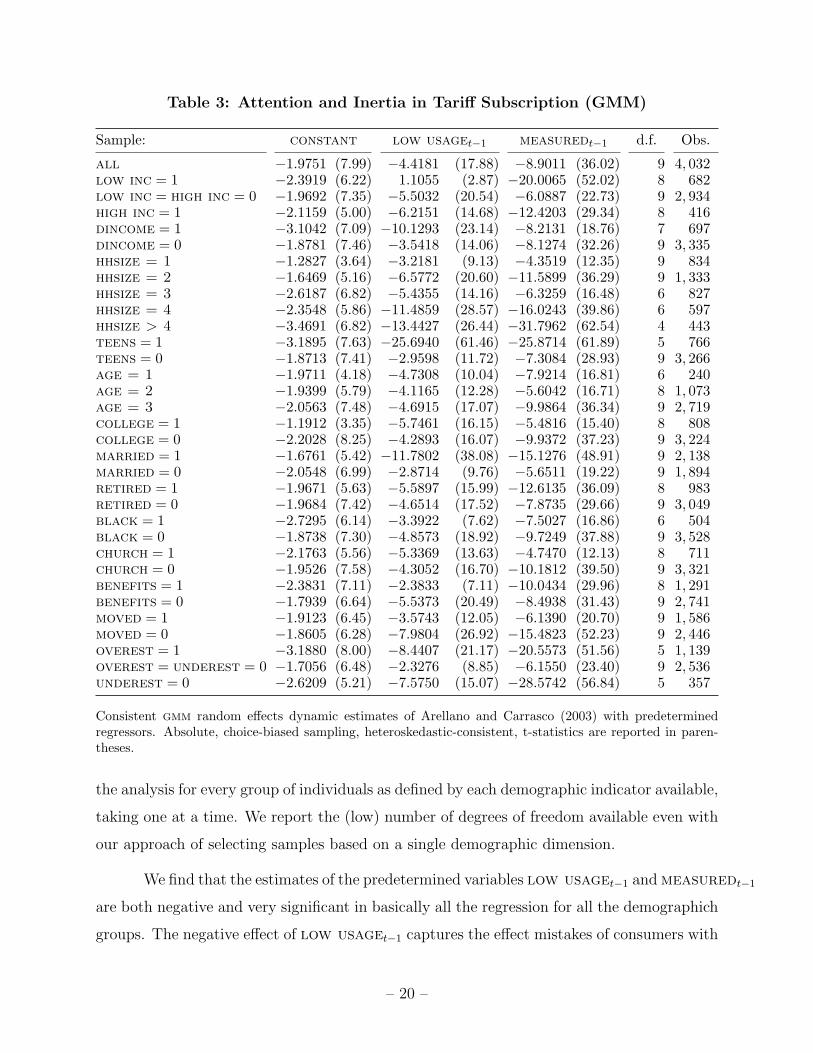
Table 3: Attention and Inertia in Tariff Subscription (GMM)

Sample: constant low usaget−1 measuredt−1 d.f. Obs.

all −1.9751 (7.99) −4.4181 (17.88) −8.9011 (36.02) 9 4, 032low inc = 1 −2.3919 (6.22) 1.1055 (2.87) −20.0065 (52.02) 8 682low inc = high inc = 0 −1.9692 (7.35) −5.5032 (20.54) −6.0887 (22.73) 9 2, 934high inc = 1 −2.1159 (5.00) −6.2151 (14.68) −12.4203 (29.34) 8 416dincome = 1 −3.1042 (7.09) −10.1293 (23.14) −8.2131 (18.76) 7 697dincome = 0 −1.8781 (7.46) −3.5418 (14.06) −8.1274 (32.26) 9 3, 335hhsize = 1 −1.2827 (3.64) −3.2181 (9.13) −4.3519 (12.35) 9 834hhsize = 2 −1.6469 (5.16) −6.5772 (20.60) −11.5899 (36.29) 9 1, 333hhsize = 3 −2.6187 (6.82) −5.4355 (14.16) −6.3259 (16.48) 6 827hhsize = 4 −2.3548 (5.86) −11.4859 (28.57) −16.0243 (39.86) 6 597hhsize > 4 −3.4691 (6.82) −13.4427 (26.44) −31.7962 (62.54) 4 443teens = 1 −3.1895 (7.63) −25.6940 (61.46) −25.8714 (61.89) 5 766teens = 0 −1.8713 (7.41) −2.9598 (11.72) −7.3084 (28.93) 9 3, 266age = 1 −1.9711 (4.18) −4.7308 (10.04) −7.9214 (16.81) 6 240age = 2 −1.9399 (5.79) −4.1165 (12.28) −5.6042 (16.71) 8 1, 073age = 3 −2.0563 (7.48) −4.6915 (17.07) −9.9864 (36.34) 9 2, 719college = 1 −1.1912 (3.35) −5.7461 (16.15) −5.4816 (15.40) 8 808college = 0 −2.2028 (8.25) −4.2893 (16.07) −9.9372 (37.23) 9 3, 224married = 1 −1.6761 (5.42) −11.7802 (38.08) −15.1276 (48.91) 9 2, 138married = 0 −2.0548 (6.99) −2.8714 (9.76) −5.6511 (19.22) 9 1, 894retired = 1 −1.9671 (5.63) −5.5897 (15.99) −12.6135 (36.09) 8 983retired = 0 −1.9684 (7.42) −4.6514 (17.52) −7.8735 (29.66) 9 3, 049black = 1 −2.7295 (6.14) −3.3922 (7.62) −7.5027 (16.86) 6 504black = 0 −1.8738 (7.30) −4.8573 (18.92) −9.7249 (37.88) 9 3, 528church = 1 −2.1763 (5.56) −5.3369 (13.63) −4.7470 (12.13) 8 711church = 0 −1.9526 (7.58) −4.3052 (16.70) −10.1812 (39.50) 9 3, 321benefits = 1 −2.3831 (7.11) −2.3833 (7.11) −10.0434 (29.96) 8 1, 291benefits = 0 −1.7939 (6.64) −5.5373 (20.49) −8.4938 (31.43) 9 2, 741moved = 1 −1.9123 (6.45) −3.5743 (12.05) −6.1390 (20.70) 9 1, 586moved = 0 −1.8605 (6.28) −7.9804 (26.92) −15.4823 (52.23) 9 2, 446overest = 1 −3.1880 (8.00) −8.4407 (21.17) −20.5573 (51.56) 5 1, 139overest = underest = 0 −1.7056 (6.48) −2.3276 (8.85) −6.1550 (23.40) 9 2, 536underest = 0 −2.6209 (5.21) −7.5750 (15.07) −28.5742 (56.84) 5 357

Consistent gmm random effects dynamic estimates of Arellano and Carrasco (2003) with predeterminedregressors. Absolute, choice-biased sampling, heteroskedastic-consistent, t-statistics are reported in paren-theses.

the analysis for every group of individuals as defined by each demographic indicator available,

taking one at a time. We report the (low) number of degrees of freedom available even with

our approach of selecting samples based on a single demographic dimension.

We find that the estimates of the predetermined variables low usaget−1 and measuredt−1

are both negative and very significant in basically all the regression for all the demographich

groups. The negative effect of low usaget−1 captures the effect mistakes of consumers with

– 20 –

Table 4: Attention and Inertia in Tariff Subscription (ML)

Sample: constant low usaget−1 measuredt−1 –lnL Obs.

all −1.7022 (77.82) 0.5388 (10.54) 3.2177 (43.13) 2329.368 4, 032low inc = 1 −1.7328 (31.75) 0.3642 (2.91) 3.2571 (17.11) 369.992 682low inc = high inc = 0 −1.6912 (66.50) 0.5764 (9.59) 3.2276 (36.69) 1722.898 2, 934high inc = 1 −1.7331 (24.92) 0.5619 (3.58) 3.1155 (14.58) 234.266 416dincome = 1 −2.0408 (30.19) 0.7973 (6.11) 3.1935 (15.58) 260.263 697dincome = 0 −1.6499 (70.87) 0.5048 (9.05) 3.2107 (39.93) 2050.425 3, 335hhsize = 1 −1.4620 (32.84) 0.3982 (4.65) 3.2386 (20.51) 648.485 834hhsize = 2 −1.6579 (44.46) 0.6111 (7.25) 3.2278 (25.10) 823.698 1, 333hhsize = 3 −1.8118 (35.60) 0.1405 (1.08) 3.0371 (18.32) 395.571 827hhsize = 4 −1.7839 (30.27) −0.0466 (0.30) 3.3795 (15.08) 284.013 597hhsize > 4 −2.1003 (24.49) 1.0141 (3.39) 3.5299 (11.53) 132.586 443teens = 1 −2.0677 (32.49) 0.6782 (3.23) 3.3546 (16.04) 242.481 766teens = 0 −1.6356 (69.51) 0.4885 (9.21) 3.1926 (39.77) 2062.152 3, 266age = 1 −1.6210 (18.73) 0.2697 (1.46) 2.9167 (11.34) 155.355 240age = 2 −1.6259 (40.43) 0.5921 (6.04) 3.0474 (23.61) 694.975 1, 073age = 3 −1.7432 (63.64) 0.5488 (8.63) 3.3448 (33.70) 1473.016 2, 719college = 1 −1.4680 (33.53) 0.4433 (4.63) 3.1072 (21.59) 622.282 808college = 0 −1.7707 (69.62) 0.5542 (9.15) 3.2418 (37.08) 1688.301 3, 224married = 1 −1.7238 (57.30) 0.6684 (8.77) 3.1634 (31.62) 1203.917 2, 138married = 0 −1.6768 (52.61) 0.4303 (6.14) 3.2856 (29.10) 1122.760 1, 894retired = 1 −1.7400 (38.21) 0.7143 (6.99) 3.3179 (19.90) 544.966 983retired = 0 −1.6904 (67.77) 0.4762 (8.04) 3.1897 (38.11) 1782.296 3, 049black = 1 −1.7978 (28.21) 1.1195 (5.49) 3.1317 (14.16) 255.872 504black = 0 −1.6886 (72.43) 0.4929 (9.26) 3.2324 (40.60) 2068.828 3, 528church = 1 −1.7209 (32.81) 0.5254 (4.27) 3.1127 (17.95) 403.143 711church = 0 −1.6982 (70.56) 0.5413 (9.63) 3.2404 (39.15) 1925.785 3, 321benefits = 1 −1.7931 (43.65) 0.4840 (5.12) 3.3164 (22.33) 646.447 1, 291benefits = 0 −1.6630 (64.23) 0.5632 (9.22) 3.1765 (36.76) 1677.616 2, 741moved = 1 −1.6377 (48.57) 0.3136 (3.94) 3.2189 (27.50) 974.101 1, 586moved = 0 −1.7471 (60.65) 0.6934 (10.36) 3.2209 (33.00) 1348.630 2, 446overest = 1 −1.9955 (41.00) 0.4503 (4.02) 3.0646 (18.91) 400.129 1, 139overest = underest = 0 −1.5673 (59.79) 0.4145 (7.44) 3.3420 (34.15) 1722.032 2, 536underest = 0 −1.8784 (23.42) 0.4421 (1.98) 2.8298 (12.32) 159.640 357

Inconsistent ml estimates. Absolute, choice-biased sampling, heteroskedastic-consistent, t-statistics arereported in parentheses.

low usage who remain on the flat tariff option or those with high enough usage that still sign

up for the optional measured tariff. Similarly, the negative effect of measuredt−1 indicates

that consumers do switch tariffs significantly and that, contrary to the hypothesis of habit

and inertia, automatic renewal of tariff subscription options does not necessarily mean that

consumers will stay in the previously chosen tariff indefinitely.17

17 Impulsiveness or random behavior, e.g., consumers choosing tariffs by flipping a fair coin everymonth, would imply a coefficient for measuredt−1 equal to zero.

– 21 –

Intuitively, as time elapses the effects of accumulated experiences, cognitive efforts,

and investments take over through the updating process embodied in E (ηi | wti) in equa-

tion (4). In this sense, these effects should become a more important determinant of tariff

choices over time. The question is whether when we take into account these effects the

results are substantially different than when we do not..

Table 4 repeats the same analysis with a standard probit regression that fails to

address the endogeneity of lagged endogenous regressors. The results are again robust across

different demographics but, quite remarkably, the sign of the effects is the opposite to the one

found in the previous table. According to the results of this misspecified model, consumers

with low demand tend to subscribe to the optional measured service once and for all since the

choice of tariff option also appears to be correlated over time. These results would support

the idea that consumers are characterized by inertia, and that low demand consumers rightly

chose the measured option and tended to stay there. Switching, if it existed, appears not

to be important according to this misspecified model. The comparison with the results in

the previous table show this erroneous conclusion is only the result of ignoring the effect of

unobserved heterogeneity associated to state dependence.

We thus conclude that individual heterogeneity and state dependence are crucial to

interpret the choice of tariff data, and that our consistent estimates do not support the idea

that consumers’ responses are determined by inertia or impulsiveness.

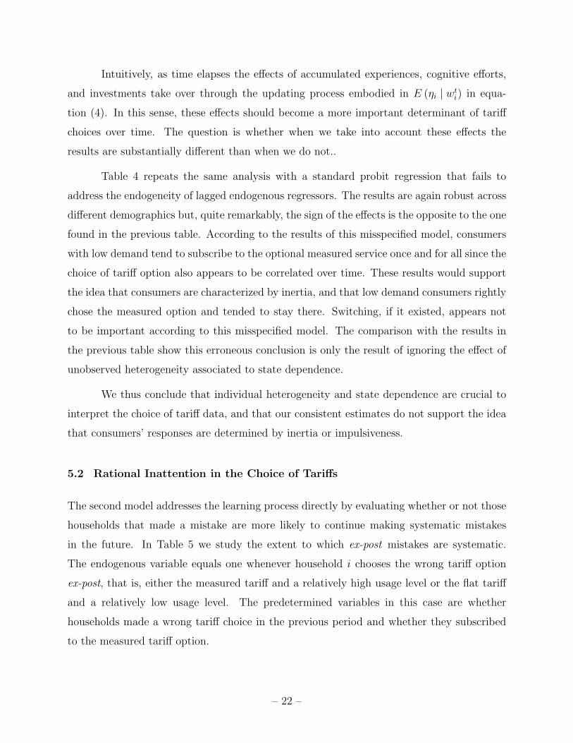
5.2 Rational Inattention in the Choice of Tariffs

The second model addresses the learning process directly by evaluating whether or not those

households that made a mistake are more likely to continue making systematic mistakes

in the future. In Table 5 we study the extent to which ex-post mistakes are systematic.

The endogenous variable equals one whenever household i chooses the wrong tariff option

ex-post, that is, either the measured tariff and a relatively high usage level or the flat tariff

and a relatively low usage level. The predetermined variables in this case are whether

households made a wrong tariff choice in the previous period and whether they subscribed

to the measured tariff option.

– 22 –

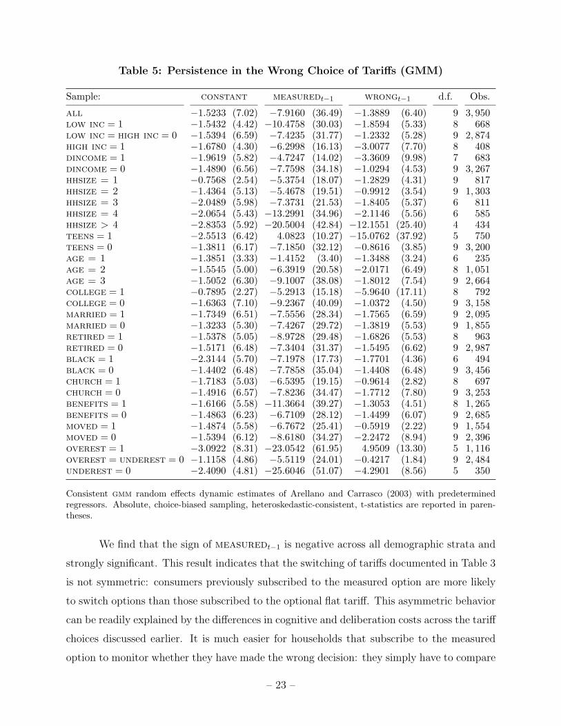
Table 5: Persistence in the Wrong Choice of Tariffs (GMM)

Sample: constant measuredt−1 wrongt−1 d.f. Obs.

all −1.5233 (7.02) −7.9160 (36.49) −1.3889 (6.40) 9 3, 950low inc = 1 −1.5432 (4.42) −10.4758 (30.03) −1.8594 (5.33) 8 668low inc = high inc = 0 −1.5394 (6.59) −7.4235 (31.77) −1.2332 (5.28) 9 2, 874high inc = 1 −1.6780 (4.30) −6.2998 (16.13) −3.0077 (7.70) 8 408dincome = 1 −1.9619 (5.82) −4.7247 (14.02) −3.3609 (9.98) 7 683dincome = 0 −1.4890 (6.56) −7.7598 (34.18) −1.0294 (4.53) 9 3, 267hhsize = 1 −0.7568 (2.54) −5.3754 (18.07) −1.2829 (4.31) 9 817hhsize = 2 −1.4364 (5.13) −5.4678 (19.51) −0.9912 (3.54) 9 1, 303hhsize = 3 −2.0489 (5.98) −7.3731 (21.53) −1.8405 (5.37) 6 811hhsize = 4 −2.0654 (5.43) −13.2991 (34.96) −2.1146 (5.56) 6 585hhsize > 4 −2.8353 (5.92) −20.5004 (42.84) −12.1551 (25.40) 4 434teens = 1 −2.5513 (6.42) 4.0823 (10.27) −15.0762 (37.92) 5 750teens = 0 −1.3811 (6.17) −7.1850 (32.12) −0.8616 (3.85) 9 3, 200age = 1 −1.3851 (3.33) −1.4152 (3.40) −1.3488 (3.24) 6 235age = 2 −1.5545 (5.00) −6.3919 (20.58) −2.0171 (6.49) 8 1, 051age = 3 −1.5052 (6.30) −9.1007 (38.08) −1.8012 (7.54) 9 2, 664college = 1 −0.7895 (2.27) −5.2913 (15.18) −5.9640 (17.11) 8 792college = 0 −1.6363 (7.10) −9.2367 (40.09) −1.0372 (4.50) 9 3, 158married = 1 −1.7349 (6.51) −7.5556 (28.34) −1.7565 (6.59) 9 2, 095married = 0 −1.3233 (5.30) −7.4267 (29.72) −1.3819 (5.53) 9 1, 855retired = 1 −1.5378 (5.05) −8.9728 (29.48) −1.6826 (5.53) 8 963retired = 0 −1.5171 (6.48) −7.3404 (31.37) −1.5495 (6.62) 9 2, 987black = 1 −2.3144 (5.70) −7.1978 (17.73) −1.7701 (4.36) 6 494black = 0 −1.4402 (6.48) −7.7858 (35.04) −1.4408 (6.48) 9 3, 456church = 1 −1.7183 (5.03) −6.5395 (19.15) −0.9614 (2.82) 8 697church = 0 −1.4916 (6.57) −7.8236 (34.47) −1.7712 (7.80) 9 3, 253benefits = 1 −1.6166 (5.58) −11.3664 (39.27) −1.3053 (4.51) 8 1, 265benefits = 0 −1.4863 (6.23) −6.7109 (28.12) −1.4499 (6.07) 9 2, 685moved = 1 −1.4874 (5.58) −6.7672 (25.41) −0.5919 (2.22) 9 1, 554moved = 0 −1.5394 (6.12) −8.6180 (34.27) −2.2472 (8.94) 9 2, 396overest = 1 −3.0922 (8.31) −23.0542 (61.95) 4.9509 (13.30) 5 1, 116overest = underest = 0 −1.1158 (4.86) −5.5119 (24.01) −0.4217 (1.84) 9 2, 484underest = 0 −2.4090 (4.81) −25.6046 (51.07) −4.2901 (8.56) 5 350

Consistent gmm random effects dynamic estimates of Arellano and Carrasco (2003) with predeterminedregressors. Absolute, choice-biased sampling, heteroskedastic-consistent, t-statistics are reported in paren-theses.

We find that the sign of measuredt−1 is negative across all demographic strata and

strongly significant. This result indicates that the switching of tariffs documented in Table 3

is not symmetric: consumers previously subscribed to the measured option are more likely

to switch options than those subscribed to the optional flat tariff. This asymmetric behavior

can be readily explained by the differences in cognitive and deliberation costs across the tariff

choices discussed earlier. It is much easier for households that subscribe to the measured

option to monitor whether they have made the wrong decision: they simply have to compare

– 23 –

Table 6: Persistence in the Wrong Choice of Tariffs (ML)

Sample: constant measuredt−1 wrongt−1 –lnL Obs.

all −1.3560 (77.89) 0.8354 (15.90) 1.3827 (34.11) 4100.418 3, 950low inc = 1 −1.3614 (32.29) 0.7466 (5.30) 1.4310 (14.83) 694.868 668low inc = high inc = 0 −1.3563 (66.20) 0.8411 (14.12) 1.3514 (28.41) 2981.507 2, 874high inc = 1 −1.3454 (25.28) 0.9418 (5.21) 1.5206 (11.69) 421.787 408dincome = 1 −1.3812 (32.85) 0.8612 (5.74) 1.1121 (11.23) 682.776 683dincome = 0 −1.3495 (70.62) 0.8126 (14.30) 1.4375 (32.20) 3410.681 3, 267hhsize = 1 −1.0573 (29.43) 0.4383 (5.27) 1.2120 (18.01) 1166.283 817hhsize = 2 −1.2785 (43.34) 0.9422 (11.49) 1.1375 (16.98) 1477.969 1, 303hhsize = 3 −1.4939 (37.19) 0.7898 (4.49) 1.6838 (14.49) 682.011 811hhsize = 4 −1.5722 (31.53) 1.2116 (6.67) 1.6317 (11.96) 446.790 585hhsize > 4 −1.7703 (27.23) 1.0586 (2.92) 1.6733 (6.69) 239.488 434teens = 1 −1.7098 (35.80) 0.3091 (1.21) 2.2813 (13.35) 452.514 750teens = 0 −1.2896 (68.05) 0.8287 (15.56) 1.2905 (30.65) 3603.162 3, 200age = 1 −1.1530 (17.50) 0.5292 (2.73) 1.4017 (9.02) 293.859 235age = 2 −1.3810 (40.53) 0.8353 (8.04) 1.5116 (18.35) 1049.965 1, 051age = 3 −1.3657 (64.14) 0.8578 (13.30) 1.3338 (27.24) 2748.582 2, 664college = 1 −1.2466 (32.83) 0.6957 (6.95) 1.6055 (19.87) 924.480 792college = 0 −1.3828 (70.51) 0.8751 (14.10) 1.2943 (27.42) 3158.056 3, 158married = 1 −1.4388 (58.24) 1.0518 (13.76) 1.3041 (20.89) 1956.573 2, 095married = 0 −1.2715 (51.37) 0.6457 (8.93) 1.4106 (26.20) 2125.535 1, 855retired = 1 −1.3772 (38.69) 0.9576 (9.58) 1.1225 (13.68) 990.614 963retired = 0 −1.3495 (67.57) 0.7849 (12.70) 1.4689 (31.31) 3100.573 2, 987black = 1 −1.5838 (29.24) 0.9984 (4.57) 1.4243 (7.95) 368.718 494black = 0 −1.3274 (71.92) 0.8187 (15.12) 1.3666 (32.70) 3720.910 3, 456church = 1 −1.3834 (32.96) 0.9122 (7.25) 1.2699 (12.88) 700.132 697church = 0 −1.3501 (70.56) 0.8196 (14.17) 1.4048 (31.58) 3398.716 3, 253benefits = 1 −1.3851 (44.59) 1.0138 (10.57) 1.1353 (15.68) 1275.014 1, 265benefits = 0 −1.3418 (63.83) 0.7387 (11.65) 1.5017 (30.40) 2812.217 2, 685moved = 1 −1.3168 (48.13) 0.7074 (8.30) 1.5454 (24.80) 1675.876 1, 554moved = 0 −1.3823 (61.16) 0.9286 (13.91) 1.2543 (23.43) 2412.525 2, 396overest = 1 −1.9257 (42.41) 1.7689 (8.15) 0.9299 (4.15) 471.857 1, 116overest = underest = 0 −1.1442 (55.42) 0.7105 (13.10) 1.2399 (29.08) 3237.562 2, 484underest = 0 −1.7267 (24.77) 0.9792 (3.23) 1.4056 (5.51) 216.562 350

Inconsistent ml estimates. Absolute, choice-biased sampling, heteroskedastic-consistent, t-statistics arereported in parentheses.

their actual bill with the $18.70 flat rate. On the contrary, households in the flat tariff would

have to actively monitor their phone calls very carefully and make more complex calculations

in order to ascertain whether or not they are paying too much for their local telephone service.

Monitoring and cognitive costs are clearly much greater for them. The asymmetric switching

behavior that we observe is thus perfectly consistent with these asymmetric differences in

complexity and cognitive costs. This result supports the implication that households that

face the less complex problem learn faster and incur in fewer mistakes.

– 24 –

We also find a negative sign for wrongt−1 which is strongly significant across all

demographic strata. This indicates that mistakes are not permanent and that the switching

between tariff options is aimed at reducing the cost of local telephone service.

These findings are important. Interestingly, they are again in sharp contrast with the

results in Table 6 of the corresponding misspecified model that fails to address the endo-

geneity of lagged endogenous regressors. The systematically positive signs and the strongly

significant effects found for measuredt−1 and wrongt−1 would indicate that households

make systematic mistakes. For instance, a household may systematically think that it is

going to consume below the threshold level but will systematically consume above it. A naıve

hyperbolic discounter who subscribed to the optional measured service as a commitment

device to limit her time on the phone would exhibit this type of systematic mistake, e.g.,

see Strotz (1956). Systematic mistakes would also be characteristic of households driven by

rational inattention.

We thus conclude that individual heterogeneity and state dependence are again crucial

to interpret the choice of tariff data, and that our consistent estimates do not support the

idea that consumers’ behavior is characterized by systematic mistakes and inattention.

5.3 Marginal Effects

Before concluding, we pursue further the result that mistakes are a transitory phenomenon,

and compute the marginal effects associated with the transition among different states.

Arellano and Carrasco (2003) show that the probability of subscribing to the wrong tariff

plan when we compare two states zit = z0 and zit = z1 changes by the proportion:

4t =1

N

N∑i=1

{Φ

(σ−1

t β(z1−zit

)+Φ−1

[ht

(wt

i

)])−Φ

(σ−1

t β(z0−zit

)+Φ−1

[ht

(wt

i

)])}.

(10)

Since the evaluation depends on the history of past choices ωti , these marginal effects

are different for each month of the sample. Table 7 presents four marginal effects evaluated

in October, November, December, as well as the average effect over the Fall.18 The first

18 These four transitions exhaust the relevant effects to be reported. To compute the marginal effectsof going in the opposite direction, just reverse the sign of the corresponding effect in Table 7.

– 25 –

Table 7: Marginal Effects

Previous Transition October November December Fall

From (Flat,Right) to (Flat,Wrong) −11.60 −6.52 −4.27 −7.46From (Measured,Right) to (Measured,Wrong) −0.01 −1.67 −2.13 −1.27From (Flat,Right) to (Measured,Right) −17.73 −17.82 −11.64 −15.73From (Flat,Wrong) to (Measured,Wrong) −6.13 −12.98 −9.49 −9.53

Percent change in the probability of choosing the current tariff option wrongly conditional on eachtransition among states.

two rows show the change in probability of choosing wrongly if consumers chose wrongly in

the previous month. The first row indicates that this probability decreases on average by

7.46% if consumers subscribed to the flat tariff option while the second row shows that this

probability decreases by 1.27% had they subscribed to the measured tariff option. Thus,

regardless of the choice of tariff, it is less likely that they make another mistake in their

choice of tariffs.

Similarly, the last two rows report the change in probability of choosing wrongly

if consumers subscribed to the optional measured service in the previous month. This

probability falls by 15.73% if consumers subscribed correctly to the optional measured service

in the previous month and by 9.53% if they subscribed wrongly to the optional measured

service. Thus, consistent with the asymmetry in the complexity of the problems discussed

earlier, the probability of making a mistake is substantially lower after subscribing to the

measured option than after subscribing to the flat tariff. This decrease in probability is more

important for those with low demand for which the measured service is the least expensive

option than for those with an usage pattern above the threshold of $18.70.

Finally, it is important to note that in analyzing these marginal effects, wrong

equals 1 when consumers pay any positive amount above the cost of the alternative option.

We repeat the analysis for different thresholds in increments of 5 cents from $0.00 to $4.00

in order to measure whether this change in the probability varies significantly with the

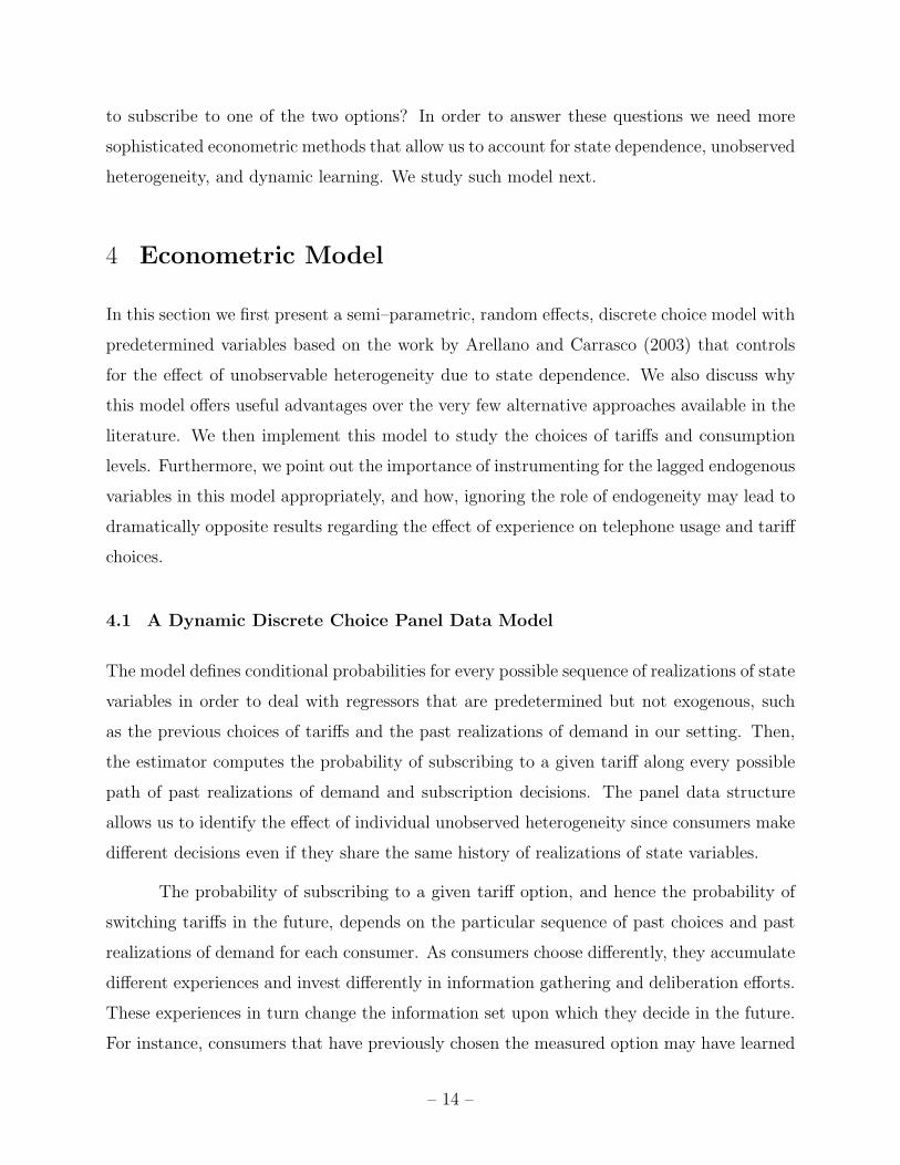
magnitude of the mistake. Figure 1 reports the average marginal effects for the Fall.

Interestingly, marginal effects experience an abrupt jump in the first 25-30 cents and remain

mostly constant once consumers realize a mistake above these 25-30 cents. Recall that under

the measured service option consumers are not billed for the $5 allowance unless their usage

– 26 –

Fig

ure

1:

Marg

inalEffect

sat

Diff

ere

nt

Mis

take

Thre

shold

s

Fig

ure

3. M

arg

inal

Eff

ects

-7.0

-6.5

-6.0

-5.5

-5.0

-4.5

-4.0

-3.5

-3.0

-2.5

-2.0

0.00

0.25

0.50

0.75

1.00

1.25

1.50

1.75

2.00

2.25

2.50

2.75

3.00

3.25

3.50

3.75

4.00

Fro

m (

0,0)

to (

0,1)

Percentage Change of Probability

-1.4

-1.2-1

-0.8

-0.6

-0.4

-0.2

0.00

0.25

0.50

0.75

1.00

1.25

1.50

1.75

2.00

2.25

2.50

2.75

3.00

3.25

3.50

3.75

4.00

Fro

m (

1,0)

to (

1,1)

Percentage Change of Probability

-15.

6

-15.

4

-15.

2

-15.

0

-14.

8

-14.

6

-14.

4

-14.

2

0.00

0.25

0.50

0.75

1.00

1.25

1.50

1.75

2.00

2.25

2.50

2.75

3.00

3.25

3.50

3.75

4.00

Fro

m (

0,0)

to (

1,0)

Percentage Change of Probability

-13.

0

-12.

5

-12.

0

-11.

5

-11.

0

-10.

5

-10.

0

-9.5

0.00

0.25

0.50

0.75

1.00

1.25

1.50

1.75

2.00

2.25

2.50

2.75

3.00

3.25

3.50

3.75

4.00

Fro

m (

0,1)

to (

1,1)

Percentage Change of Probability

– 27 –

is above $19.02. This is 32 cents more than the $18.70 cost of the flat tariff option. We find

it remarkable that this amount is almost identical to 25-30 cents.

6 Concluding Remarks

The systematic analysis of individual responses to changes in the environment is important

for understanding the determinants of attention and inattention, and the extent and forma-

tion of rationality. The natural setting of the Kentucky tariff experiment and a rich panel

dataset that is free from a number of critical obstacles that may explain the lack of empirical

studies in the literature have allowed us to uncover households’ responses in isolation from

a number of conflicting considerations which generally exist in other circumstances.

We find that households recognize that choices today affect their utilities in the future

and actively react to a new option despite potential savings of very small magnitude. They

make no systematic mistakes. Their reactions, however, are not symmetric. Households who

face a more complex and cognitively more expensive tariff problem learn more slowly and

are more likely to make mistakes than households that face a simpler tariff choice problem.

The fact that the evidence turns out to be drastically different when lagged endogenous

variables and unobserved heterogeneity are appropriately treated indicates that they play

an important role in the dynamic learning process.

When and why people are attentive or inattentive and, when they are attentive, when

and why people get it right or wrong, are fundamental questions for our understanding of

human decision making. We cannot claim, and we do not claim, that we should expect

that the results we have obtained will systematically generalize to other settings. This

is an empirical question whose answer depends on the degree of complexity, the costs of

information, the size of incentives, and all other characteristics of the specific problem and

environment under study. What we hope, however, is that the analysis in the current paper

will begin to pave the way for an empirically based science of decision making which together

with theoretical and experimental work on cognitive processes will significantly improve our

understanding of when and how decision makers think about real life problems.

– 28 –

References

Akerlof, G. A. and W. T. Dickens (1982): “The Economic Consequences of CognitiveDissonance.” American Economic Review, 72, 307–319.

Akerlof, G. A. and J. L. Yellen (1982): “Rational Models of Irrational Behavior.”American Economic Review, 77, 137–142.

Amemiya, T. (1985): Advanced Econometrics. Cambridge, MA: Harvard University Press.

Americks, J., A. Caplin, and J. Leahy (2003): “Wealth Accumulation and the Propen-sity to Plan.” Quarterly Journal of Economics, 118, 1007–1047.

Arellano, M. and O. Bover (1995): “Another Look at the Instrumental VariableEstimation of Error-Components Model.” Journal of Econometrics, 68, 29–51.

Arellano, M. and R. Carrasco (2003): “Binary Choice Panel Data Models withPredetermined Variables.” Journal of Econometrics, 115, 125–157.

Arellano, M. and B. E. Honore (2001): “Panel Data Models: Some Recent Develop-ments.” In J. E. Heckman and E. Leamer (eds.): Handbook of Econometrics, vol. V.North-Holland.

Arrow, K. J. (1987): “Rationality of Self and Others in an Economic System.” In R. M.Hogarth and M. W. Reder (eds.): Rational Choice. The Contrast Between Economicsand Psychology. Chicago, IL: Chicago University Press.

Ball, L., N. G. Mankiw, and R. Reis (2005): “Monetary Policy for InattentiveEconomies.” Journal of Monetary Economics, 52, 703–725.

Becker, G. S. (1962): “Irrational Behavior and Economic Theory.” Journal of PoliticalEconomy, 70, 1–3.

Bolton, P. and A. Faure-Grimaud (2005a): “Thinking Ahead: Part II, SatisficingContracts.” Mimeo, Columbia University and LSE.

Bolton, P. and A. Faure-Grimaud (2005b): “Thinking Ahead: The Decision Problem.”Mimeo, Columbia University and LSE.

Carroll, C. D. (2003): “Macroeconomic Expectations of Households and ProfessionalForecasters.” Quarterly Journal of Economics, 118, 269–298.

Chamberlain, G. (1980): “Analysis of Covariance with Qualitative Data.” Review ofEconomic Studies, 47, 225–238.

Chamberlain, G. (1984): “Panel Data.” In Z. Griliches and M. D. Intriligator (eds.):Handbook of Econometrics, vol. II. New York, NY: North-Holland.

Chiappori, P.-A. and B. Salanie (2000): “Testing for Asymmetric Information inInsurance Markets.” Journal of Political Economy, 108, 56–78.

– 29 –

Conslik, J. (1996): “Why Bounded Rationality?” Journal of Economic Literature, 34,669–700.

Costa-Gomes, M. A. and V. P. Crawford (2006): “Cognition and Behavior in Two-Person Guessing Games: An Experimental Study.” American Economic Review, 96,1737–1768.

Costa-Gomes, M. A., V. P. Crawford, and B. Broseta (2006): “Cognition andBehavior in Normal-Form Games: An Experimental Study.” Econometrica, 69, 1193–1235.

Ellison, G. and D. Fudenberg (1993): “Rules of Thumb for Social Learning.” Journalof Political Economy, 101, 612–643.

Gabaix, X. and D. Laibson (2002): “The 6D Bias and the Equity Premium Puzzle.”NBER Macroeconomics Annual 2001, 257–311.

Gabaix, X., D. Laibson, G. Moloche, and S. Weinberg (2006): “Costly InformationAcquisition: Experimental Analysis of a Bounded Rationality Model.” AmericanEconomic Review, 96, 1043–1048.

Gode, D. k. and S. Sunder (1993): “Allocative Efficiency of Markets with Zero-Intelligence Traders: Market as a Partial Substitute for Individual Rationality.”Journal of Political Economy, 101, 119–137.

Hansen, L. P. and T. J. Sargent (2008): Robustness. Princeton, NJ: PrincetonUniversity Press.

Heckman, J. J. (1981): “The Incidental Parameters Problem and the Problem of InitialConditions in Estimating a Discrete Time - Discrete Data Stochastic Process.” InC. F. Manski and D. L. McFadden (eds.): Structural Analysis of Discrete Data withApplications. Cambridge, MA: MIT Press.

Honore, B. and E. Kyriazidou (2000): “Panel Data Discrete Choice Models with LaggedDependent Variables.” Econometrica, 68, 839–874.

Honore, B. and A. Lewbel (2002): “Semiparametric Binary Choice Panel Data Modelswithout Strictly Exogenous Regressors.” Econometrica, 70, 2053–2063.

Lancaster, T. (2000): “The Incidental Parameter Problem since 1948.” Journal ofEconometrics, 95, 391–413.

Lerman, S. R. and C. F. Manski (1977): “The Estimation of Choice Probabilities fromChoice Based Samples.” Econometrica, 45, 1977–1988.

Lipman, B. L. (1991): “How to Decide How to Decide How to ...: Modeling LimitedRationality.” Econometrica, 59, 1105–1125.

– 30 –

Lucas, R. E. J. (1987): “Adaptive Behavior and Economic Theory.” In R. M. Hogarthand M. W. Reder (eds.): Rational Choice. The Contrast Between Economics andPsychology. Chicago, IL: Chicago University Press.

Lusardi, A. (1999): “Information, Expectations and Savings.” In H. Aaron (ed.): Behav-ioral Dimensions of Retirement Economics. New York, NY: Rusell Sage Foundation.

Lusardi, A. (2003): “Planning and Saving for Retirement.” Mimeo, Darmouth College.

Mankiw, N. G. and R. Reis (2002): “Sticky Information versus Sticky Prices: A Proposalto Replace the New Keynesian Philips Curve.” Quarterly Journal of Economics, 117,1295–1328.

Manski, C. F. (1987): “Semiparametric Analysis of Random Effects Linear Models fromBinary Panel Data.” Econometrica, 55, 357–362.

Miravete, E. J. (2002): “Estimating Demand for Local Telephone Service with Asymmet-ric Information and Optimal Calling Plans.” The Review of Economic Studies, 69,943–971.

Miravete, E. J. (2003): “Choosing the Wrong Calling Plan? Ignorance and Learning.”American Economic Review, 93, 297–310.

Miravete, E. J. (2005): “The Welfare Performace of Sequential Pricing Mechanisms.”International Economic Review, 46, 1321–1360.

Mitchell, B. M. and I. Vogelsang (1991): Telecommunication Pricing. Theory andPractice. Cambridge, UK: Cambridge University Press.

Moscarini, G. (2004): “Limited Information Capacity as a Source of Inertia.” Journal ofEconomic Dynamics and Control, 28, 2003–2035.

Moscarini, G. and L. Smith (2001): “The Optimal Level of Experimentation.” Econo-metrica, 69, 1629–1644.

Moscarini, G. and L. Smith (2002): “The Law of Large Demand for Information.”Econometrica, 70, 2351–2366.

Narayanan, S., P. K. Chintagunta, and E. J. Miravete (2007): “The Role ofSelf Selection, Usage Uncertainty and Learning in the Demand for Local TelephoneService.” Quantitative Marketing and Economics, 5, 1–34.

Newey, W. K. (1994): “The Asymptotic Variance of Semiparametric Estimators.” Econo-metrica, 62, 1349–1382.

Neyman, j. and E. L. Scott (1948): “Consistent Estimation from Partially ConsistentObservations.” Econometrica, 16, 1–32.

Reis, R. (2006a): “Inattentive Consumers.” Journal of Monetary Economics, 53, 1761–1800.

– 31 –

Reis, R. (2006b): “Inattentive Producers.” Review of Economic Studies, 73, 793–821.

Rubinstein, A. (1998): Modeling Bounded Rationality. Cambride, MA: MIT Press.

Sargent, T. J. (1993): Bounded Rationality in Macroeconomics. Oxford, UK: OxfordUniversity Press.

Savage, L. J. (1954): The Foundations of Statistics. New York, NY: Wiley & Sons.

Shapiro, M. D. and J. Slemrod (1995): “Consumer Response to the Timing of Income:Evidence from a Change in Tax Witholding.” American Economic Review, 85, 274–283.

Sims, C. A. (2003): “Implications of Rational Inattention.” Journal of Monetary Eco-nomics, 50, 665–690.

Sims, H. A. (1955): “A Behavioral Model of Rational Choice.” Quarterly Journal ofEconomics, 69, 99–118.

Sims, H. A. (1987): “Rationality in Psychology and Economics.” In R. M. Hogarthand M. W. Reder (eds.): Rational Choice. The Contrast Between Economics andPsychology. Chicago, IL: Chicago University Press.

Stigler, G. J. and G. S. Becker (1977): “De Gustibus Non Est Disputandum.”American Economic Review, 67, 76–90.

Strotz, R. H. (1956): “Myopia and Inconsistency in Dynamic Utility Maximization.”Review of Economic Studies, 23, 165–180.

Tobin, J. (1982): “Money and Finance in the Macroeconomic Process.” Journal of Money,Credit and Banking, 14, 171–204.

– 32 –